GENETICS AND CRITICAL ILLNESS INSURANCE UNDERWRITING ...
319
GENETICS AND CRITICAL ILLNESS INSURANCE UNDERWRITING: MODELS FOR BREAST CANCER AND OVARIAN CANCER AND FOR CORONARY HEART DISEASE AND STROKE By Chessman Tavarwisa Wekwete Submitted for the Degree of Doctor of Philosophy at Heriot-Watt University on Completion of Research in the Department of Actuarial Mathematics & Statistics November 2002. This copy of the thesis has been supplied on the condition that anyone who consults it is understood to recognise that the copyright rests with its author and that no quo- tation from the thesis and no information derived from it may be published without the prior written consent of the author or the university (as may be appropriate).
Transcript of GENETICS AND CRITICAL ILLNESS INSURANCE UNDERWRITING ...

GENETICS AND CRITICAL ILLNESS INSURANCE
UNDERWRITING: MODELS FOR BREAST CANCER
AND OVARIAN CANCER AND FOR CORONARY
HEART DISEASE AND STROKE
By
Chessman Tavarwisa Wekwete
Submitted for the Degree of
Doctor of Philosophy
at Heriot-Watt University
on Completion of Research in the
Department of Actuarial Mathematics & Statistics
November 2002.
This copy of the thesis has been supplied on the condition that anyone who consults
it is understood to recognise that the copyright rests with its author and that no quo-
tation from the thesis and no information derived from it may be published without
the prior written consent of the author or the university (as may be appropriate).

I hereby declare that the work presented in this the-
sis was carried out by myself at Heriot-Watt University,
Edinburgh, except where due acknowledgement is made,
and has not been submitted for any other degree.
Chessman Tavarwisa Wekwete (Candidate)
Professor Howard R. Waters (Supervisor)
Professor Angus S. Macdonald (Supervisor)
Date
ii

Preface
Throughout the 1970s and 1980s the impact of lifestyle and medical advances on
longevity and the impact of AIDS on mortality brought to the fore the need for
the insurance industry constantly to monitor mortality trends. Given the long term
nature of life insurance contracts, early detection of moves in mortality is important
if the industry is to avoid selling a lot of bad business or even making significant
losses due to anti-selection. Life insurers need to keep an eye out for any area of life
from where a significant shift of their mortality or morbidity experience could arise.
Human genetics is one such area. Advances in genetic knowledge have been
largely funded on the promise of discoveries that will improve prevention and treat-
ment of diseases. The prevention of diseases is largely underpinned by genetically
determined knowledge of increased risk of the disease. Possible misuse of this predic-
tive function (real or perceived) of genetic knowledge to the disadvantage of insurers
is a central aspect of the current genetics and insurance debate. It is clear that the
decision on the use or non-use of genetics in insurance underwriting will not be made
by the insurance industry, at least not on its own. It is actually the fact that the
insurance industry has to prove how it would be significantly disadvantaged by any
misuse of genetic information.
iii

To contribute information for the debate this thesis aims to assess the costs of
insurance that are likely to arise under situations where use of genetic information
in underwriting is allowed, and when it is not. We focus on genetic information
related to breast cancer and ovarian cancer and to coronary heart disease and stroke.
For breast cancer and ovarian cancer genes called BRCA1 and BRCA2 have been
identified as associated with the risk of these two disorders. Significant research
on these genes has been published which allows us to make a relatively detailed
assessment on how insurance costs differ if use of this genetic information is allowed
or disallowed for underwriting purposes.
We await more advances on the genetics of coronary heart disease and stroke.
In the thesis we produce a model for use in calculating insurance costs associated
with these two disorders. We use the model to assess how genetic knowledge may
change these costs.
iv
Contents
Preface iii
Acknowledgements xx
Abstract xxi
Introduction 1
1 Background 41.1 Risk and life underwriting . . . . . . . . . . . . . . . . . . . . . . . . 4
1.1.1 Risk classification . . . . . . . . . . . . . . . . . . . . . . . . . 51.1.2 Underwriting . . . . . . . . . . . . . . . . . . . . . . . . . . . 9
1.2 Genetics . . . . . . . . . . . . . . . . . . . . . . . . . . . . . . . . . . 121.2.1 Cells, chromosomes and DNA . . . . . . . . . . . . . . . . . . 121.2.2 Duplicating genetic information for protein synthesis . . . . . 141.2.3 Duplicating genetic information for creating new cells . . . . . 141.2.4 Mutations and disorders . . . . . . . . . . . . . . . . . . . . . 151.2.5 Genetic testing and insurance . . . . . . . . . . . . . . . . . . 16
1.3 Continuous time Markov models . . . . . . . . . . . . . . . . . . . . . 201.4 Epidemiological statistics . . . . . . . . . . . . . . . . . . . . . . . . . 23
1.4.1 Longitudinal studies . . . . . . . . . . . . . . . . . . . . . . . 241.4.2 Retrospective case-control studies . . . . . . . . . . . . . . . . 291.4.3 Cross-sectional studies . . . . . . . . . . . . . . . . . . . . . . 30
1.5 Critical illness insurance . . . . . . . . . . . . . . . . . . . . . . . . . 30
2 Genetic and family history models for breast and ovarian cancer 342.1 Breast cancer . . . . . . . . . . . . . . . . . . . . . . . . . . . . . . . 342.2 Ovarian cancer . . . . . . . . . . . . . . . . . . . . . . . . . . . . . . 362.3 BCOC underwriting . . . . . . . . . . . . . . . . . . . . . . . . . . . 382.4 Genetics of breast cancer and ovarian cancer . . . . . . . . . . . . . . 41
2.4.1 BRCA1 and BRCA2 susceptibility genes . . . . . . . . . . . . 412.4.2 BCOC genetics in clinical practice . . . . . . . . . . . . . . . . 462.4.3 BCOC genetics applied to investigations into the impact of
BCOC on insurance . . . . . . . . . . . . . . . . . . . . . . . 472.5 Determining carrier probabilities . . . . . . . . . . . . . . . . . . . . . 48
2.5.1 Definitions . . . . . . . . . . . . . . . . . . . . . . . . . . . . . 492.5.2 Model for relative’s BCOC history . . . . . . . . . . . . . . . 532.5.3 Calculation of carrier probabilities . . . . . . . . . . . . . . . . 69
v
2.5.4 Carrier probabilities with known family structure . . . . . . . 732.5.5 Distribution of family structure . . . . . . . . . . . . . . . . . 812.5.6 Carrier probabilities with unknown family structure . . . . . . 872.5.7 Effect of lower BRCA1 and BRCA2 penetrance . . . . . . . . 932.5.8 Summary of model features . . . . . . . . . . . . . . . . . . . 95
3 Application of the breast and ovarian cancer model to Critical Ill-ness insurance 1003.1 The applicant’s model . . . . . . . . . . . . . . . . . . . . . . . . . . 101
3.1.1 Incidence rates of breast cancer . . . . . . . . . . . . . . . . . 1013.1.2 Incidence rates of ovarian cancer . . . . . . . . . . . . . . . . . 1023.1.3 Incidence of other critical illness and surviving 28 days . . . . 1023.1.4 Mortality . . . . . . . . . . . . . . . . . . . . . . . . . . . . . 114
3.2 Cost of insurance . . . . . . . . . . . . . . . . . . . . . . . . . . . . . 1163.2.1 Insurance costs by genotype . . . . . . . . . . . . . . . . . . . 1173.2.2 Premium rating with complete knowledge of the family history
and structure . . . . . . . . . . . . . . . . . . . . . . . . . . . 1203.2.3 Premium rating with incomplete knowledge of the family his-
tory and structure . . . . . . . . . . . . . . . . . . . . . . . . 1233.2.4 The effect of lower BRCA1 and BRCA2 penetrance . . . . . . 127
3.3 Potential for adverse selection . . . . . . . . . . . . . . . . . . . . . . 1293.4 Discussion . . . . . . . . . . . . . . . . . . . . . . . . . . . . . . . . . 139
4 Coronary heart disease and stroke 1434.1 Coronary heart disease . . . . . . . . . . . . . . . . . . . . . . . . . . 1434.2 Stroke . . . . . . . . . . . . . . . . . . . . . . . . . . . . . . . . . . . 1444.3 Epidemiology and risk factors . . . . . . . . . . . . . . . . . . . . . . 145
4.3.1 Body mass index . . . . . . . . . . . . . . . . . . . . . . . . . 1464.3.2 Smoking . . . . . . . . . . . . . . . . . . . . . . . . . . . . . . 1474.3.3 Hypertension . . . . . . . . . . . . . . . . . . . . . . . . . . . 1474.3.4 Cholesterol . . . . . . . . . . . . . . . . . . . . . . . . . . . . 1484.3.5 Diabetes . . . . . . . . . . . . . . . . . . . . . . . . . . . . . . 150
4.4 CHD and stroke underwriting for CI insurance . . . . . . . . . . . . . 1524.5 The genetics of CHD and stroke . . . . . . . . . . . . . . . . . . . . . 154
4.5.1 Hypertension . . . . . . . . . . . . . . . . . . . . . . . . . . . 1554.5.2 Hypercholesterolaemia . . . . . . . . . . . . . . . . . . . . . . 1564.5.3 Diabetes . . . . . . . . . . . . . . . . . . . . . . . . . . . . . . 157
4.6 Models for the development of CHD, stroke and the risk factors . . . 1594.6.1 The Framingham Heart Study data . . . . . . . . . . . . . . . 1604.6.2 Model for incidence of CHD and incidence of stroke . . . . . . 1684.6.3 Models for movement between blood pressure categories . . . 1764.6.4 Models for movement between cholesterol levels . . . . . . . . 1814.6.5 Models for movement between blood sugar levels . . . . . . . 190
4.7 Discussion of risk factor models . . . . . . . . . . . . . . . . . . . . . 1934.7.1 Blood pressure . . . . . . . . . . . . . . . . . . . . . . . . . . 1934.7.2 Cholesterol . . . . . . . . . . . . . . . . . . . . . . . . . . . . 1974.7.3 Diabetes . . . . . . . . . . . . . . . . . . . . . . . . . . . . . . 200
vi
4.8 Assessment of CHD and stroke model adequacy . . . . . . . . . . . . 2024.8.1 Comparison of CHD and stroke incidence rates . . . . . . . . 2034.8.2 Comparison of CHD and stroke probability rates . . . . . . . 205
5 Application of the CHD and stroke model to Critical Illness insur-ance 2145.1 The critical illness insurance model . . . . . . . . . . . . . . . . . . . 2145.2 Parameters for the model . . . . . . . . . . . . . . . . . . . . . . . . . 216
5.2.1 Mortality . . . . . . . . . . . . . . . . . . . . . . . . . . . . . 2165.2.2 Onset of risk factors . . . . . . . . . . . . . . . . . . . . . . . 2165.2.3 CHD . . . . . . . . . . . . . . . . . . . . . . . . . . . . . . . . 2175.2.4 Stroke . . . . . . . . . . . . . . . . . . . . . . . . . . . . . . . 2175.2.5 Other CI events . . . . . . . . . . . . . . . . . . . . . . . . . . 217
5.3 Costs of critical illness insurance . . . . . . . . . . . . . . . . . . . . . 2335.3.1 Premium rating by subpopulation and risk factor status . . . 2345.3.2 Premium ratings under hypothetical assumptions of genetic
influence of incidence rates. . . . . . . . . . . . . . . . . . . . 2425.4 Discussion . . . . . . . . . . . . . . . . . . . . . . . . . . . . . . . . . 252
5.4.1 Relative importance of types of mutations . . . . . . . . . . . 2525.4.2 Potential for adverse selection . . . . . . . . . . . . . . . . . . 2595.4.3 Ongoing assessment of the impact of genetic advances on in-
surability . . . . . . . . . . . . . . . . . . . . . . . . . . . . . 2605.4.4 Application to insurance underwriting . . . . . . . . . . . . . 260
6 Conclusions and further research 2626.1 Breast and Ovarian Cancer . . . . . . . . . . . . . . . . . . . . . . . . 262
6.1.1 Conclusions . . . . . . . . . . . . . . . . . . . . . . . . . . . . 2626.1.2 Contribution . . . . . . . . . . . . . . . . . . . . . . . . . . . 2636.1.3 Further research . . . . . . . . . . . . . . . . . . . . . . . . . . 264
6.2 CHD and Stroke . . . . . . . . . . . . . . . . . . . . . . . . . . . . . 2656.2.1 Conclusions and contribution . . . . . . . . . . . . . . . . . . 2656.2.2 Further research . . . . . . . . . . . . . . . . . . . . . . . . . . 266
A BC cases and exposed to risk 268
B OC cases and exposed to risk 269
C Mortality adjustment data set 270
D ‘Other cancers’ incidence data 271
E Cancer incidence data: Females 272
F Cancer incidence data: Males 273
G Mortality adjustment factors 274
H Cardiovascular risk profiles 277
vii

I Variance-covariance matrices 279
J ESRD cases and exposed to risk 283
References 284
viii
List of Tables
1.1 Typical medical limits for underwriting. . . . . . . . . . . . . . . . . . 112.2 Manchester staging system given in Souhami and Tobias (1998). . . . 352.3 Examples of critical illness underwriting of breast cancer family history. 392.4 Examples of critical illness underwriting of ovarian cancer family history. 402.5 Cumulative probabilities of BC under the C.A.S.H. model. (Source:
Claus et al. (1991).) . . . . . . . . . . . . . . . . . . . . . . . . . . . . 412.6 Cumulative probabilities of BC for a woman with one first degree
relative with BC (under the C.A.S.H. model). (Source: Claus et al.(1994).) . . . . . . . . . . . . . . . . . . . . . . . . . . . . . . . . . . 42
2.7 BC and OC penetrance of BRCA1 by age 70. . . . . . . . . . . . . . 432.8 Penetrance of BRCA1. (Source: Ford et al. (1998).) . . . . . . . . . . 432.9 Penetrance of BRCA2. (Source: Ford et al. (1998).) . . . . . . . . . . 442.10 Estimated frequencies of BRCA1 and BRCA2 mutations. . . . . . . . 442.11 The population frequencies of the four genotypes (0, 0), (0, 1), (1, 0)
and (1, 1), given the low and high estimates of mutation frequenciesfrom Parmigiani et al. (1998). . . . . . . . . . . . . . . . . . . . . . . 50
2.12 Incidence of BC and OC in BRCA1 mutation carriers. . . . . . . . . 612.13 Modelled cumulative risks of breast cancer, and breast or ovarian
cancer in BRCA1 mutation carriers compared with observed ratesand 95% confidence intervals in Table 2.8. . . . . . . . . . . . . . . . 63
2.14 Cumulative risk of OC only in BRCA1 mutation carriers . . . . . . . 632.15 Modelled cumulative risks of breast cancer and ovarian cancer in
BRCA2 mutation carriers compared with observed rates and 95%confidence intervals in Table 2.9. . . . . . . . . . . . . . . . . . . . . . 67
2.16 Distribution of familial genotypes for families of size 2. ‘Low’ esti-mates of mutation frequencies. . . . . . . . . . . . . . . . . . . . . . . 72
2.17 The effect of the number of sisters on probabilities of the applicant’sgenotype, given zero or one affected relatives. Applicant age 30. Uses‘high’ mutation frequencies. . . . . . . . . . . . . . . . . . . . . . . . 76
2.18 The effect of the number of sisters on probabilities of the applicant’sgenotype, given two or more affected relatives. Applicant age 30.Uses ‘high’ mutation frequencies. . . . . . . . . . . . . . . . . . . . . 77
2.19 The applicant’s genotype probabilities, given one relative with BCbefore age 50, for M = 4 or 6. Applicant age 30. ‘High’ estimates ofmutation frequencies. . . . . . . . . . . . . . . . . . . . . . . . . . . . 78
ix
2.20 The applicant’s genotype probabilities, given two relatives with BCbefore age 50, for M = 4 or 6. Applicant age 30. ‘High’ estimates ofmutation frequencies. . . . . . . . . . . . . . . . . . . . . . . . . . . . 79
2.21 The applicant’s genotype probabilities, given two or more relativeswith BC before age 50, for M = 4 or 6. Applicant age 30. ‘High’estimates of mutation frequencies. . . . . . . . . . . . . . . . . . . . . 79
2.22 The applicant’s genotype probabilities, given two relatives with BCbefore age 50, for M = 4 or 6. Applicant age 50. ‘High’ estimates ofmutation frequencies. . . . . . . . . . . . . . . . . . . . . . . . . . . . 80
2.23 The applicant’s genotype probabilities, given two relatives with BCbefore age 50, for M = 4 or 6. Applicant age 30. ‘Low’ estimates ofmutation frequencies. . . . . . . . . . . . . . . . . . . . . . . . . . . . 81
2.24 The applicant’s genotype probabilities, given two relatives with BCat ages 50–65, for M = 4 or 6. Applicant age 30. ‘High’ estimates ofmutation frequencies. . . . . . . . . . . . . . . . . . . . . . . . . . . . 81
2.25 Distribution of final or expected numbers of children born to womenborn in England and Wales in 1930–44. (Source: Shaw (1990).) . . . 84
2.26 Distribution of numbers of children according to year of mother’smarriage, England and Wales. (Source: O.P.C.S. (1983).) . . . . . . . 84
2.27 Distribution of the number of the applicant’s sisters and aunts. . . . . 862.28 The effect of the maximum family size, M , on probabilities of the
applicant’s genotype, given two relatives with BC before age 50 andunknown (M,X). Applicant age 30. ‘High’ estimates of mutationfrequencies. . . . . . . . . . . . . . . . . . . . . . . . . . . . . . . . . 88
2.29 The effect of the family history (BC before age 50 only) and maximumfamily size, M , on probabilities of the applicant’s genotype, unknown(M,X). ‘High’ estimates of mutation frequencies. . . . . . . . . . . . 89
2.30 The proportions of carrier probabilities given known family struc-tures in Tables 2.19 and 2.20 to their representative values if familystructure is assumed unknown in Table 2.29. . . . . . . . . . . . . . . 90
2.31 The effect of the family history (BC before age 50) on probabilitiesof the applicant’s genotype, unknown (M,X). Maximum family sizeM = 9. ‘Low’ estimates of mutation frequencies. . . . . . . . . . . . . 91
2.32 The effect of the family history (BC at ages 50–65) on probabilitiesof the applicant’s genotype, unknown (M,X). Maximum family sizeM = 9. ‘High’ estimates of mutation frequencies. . . . . . . . . . . . 92
2.33 The effect of the family history (BC at ages 50–65) on probabilitiesof the applicant’s genotype, unknown (M,X). Maximum family sizeM = 9. ‘Low’ estimates of mutation frequencies. . . . . . . . . . . . . 92
2.34 The effect of the family history (OC before age 50) on probabilitiesof the applicant’s genotype, unknown (M,X). Maximum family sizeM = 9. ‘High’ estimates of mutation frequencies. . . . . . . . . . . . 93
2.35 The effect of the family history (OC before age 50) on probabilitiesof the applicant’s genotype, unknown (M,X). Maximum family sizeM = 9. ‘Low’ estimates of mutation frequencies. . . . . . . . . . . . . 94
x

2.36 The effect of the family history (OC at ages 50–65) on probabilitiesof the applicant’s genotype, unknown (M,X). Maximum family sizeM = 9. ‘High’ estimates of mutation frequencies. . . . . . . . . . . . 95
2.37 The effect of the family history (OC at ages 50–65) on probabilitiesof the applicant’s genotype, unknown (M,X). Maximum family sizeM = 9. ‘Low’ estimates of mutation frequencies. . . . . . . . . . . . . 96
2.38 The applicant’s genotype probabilities, given one relative with BCbefore age 50, for M = 4 or 6. Applicant age 30. ‘High’ estimatesof mutation frequencies. BC and OC excess incidence rates of at-riskgenotypes at 100%, 50% and 25% of previous estimates. . . . . . . . . 97
2.39 The applicant’s genotype probabilities, given two relatives with BCbefore age 50, for M = 4 or 6. Applicant age 30. ‘High’ estimatesof mutation frequencies. BC and OC excess incidence rates of at-riskgenotypes at 100%, 50% and 25% of previous estimates. . . . . . . . . 98
2.40 The effect of the family history (BC before age 50 only) and maximumfamily size, M , on probabilities of the applicant’s genotype, unknown(M,X). ‘High’ estimates of mutation frequencies. BC and OC excessincidence rates of at-risk genotypes at 100%, 50% and 25% of previousestimates. . . . . . . . . . . . . . . . . . . . . . . . . . . . . . . . . . 99
3.41 Exposed to risk, observed number of cases and crude incidence ratesof first-ever heart attack (ICD 410 and 414) amoung women. (Source:McCormick et al. (1995).) . . . . . . . . . . . . . . . . . . . . . . . . 105
3.42 Incidence rates of first-ever stroke among women. (Source: Stewartet al. (1999).) . . . . . . . . . . . . . . . . . . . . . . . . . . . . . . . 109
3.43 Exposed to risk, cases and incidence rates of stroke from the M.S.G.P.study ( Source: McCormick et al. (1995)) and incidence rates of strokefrom the O.C.S.P. ( Source: Bamford et al. (1988).) . . . . . . . . . . 110
3.44 Incidence rates (per 1,000) of CI claims by cause, for females in theU.K. in 1991–97. (Source: Dinani et al. (2000).) . . . . . . . . . . . . 114
3.45 Mortality data for adjusting ELT15F for CI causes of death. . . . . . 1153.46 Expected present value (EPV) of Critical Illness cover of £1, depend-
ing on BRCA1 and BRCA2 genotype, and based on ‘low’ and ‘high’estimates of mutation frequencies. . . . . . . . . . . . . . . . . . . . . 117
3.47 Expected present value (EPV) of an annuity of £1 per year payablecontinuously while in the ‘healthy’ state of Figure 3.16, dependingon BRCA1 and BRCA2 genotype, and based on ‘low’ and ‘high’ es-timates of mutation frequencies. . . . . . . . . . . . . . . . . . . . . . 118
3.48 Level net premium for Critical Illness cover of £1, depending onBRCA1 and BRCA2 genotype, and based on ‘low’ and ‘high’ esti-mates of mutation frequencies. . . . . . . . . . . . . . . . . . . . . . . 119
3.49 Level net premium for Critical Illness cover of £1, depending onBRCA1 and BRCA2 genotype, based on ‘high’ estimates of muta-tion frequencies, as a percentage of the aggregate premium. . . . . . . 119
3.50 Level net premium for £1 CI benefit, given one relative with BCbefore age 50, for M = 4 or 6. ‘High’ estimates of mutation frequencies.121
3.51 Level net premium for £1 CI benefit, given one relative with BCbefore age 50, for M = 4 or 6. ‘Low’ estimates of mutation frequencies.122
xi

3.52 Level net premium for £1 CI benefit, given two relatives with BCbefore age 50, for M = 4 or 6. ‘High’ estimates of mutation frequencies.122
3.53 Level net premium for £1 CI benefit, given two relatives with BCbefore age 50, for M = 4 or 6. ‘Low’ estimates of mutation frequencies.123
3.54 Level net premium for £1 CI benefit, given two or more relativeswith BC before age 50, for M = 4 or 6. ‘High’ estimates of mutationfrequencies. . . . . . . . . . . . . . . . . . . . . . . . . . . . . . . . . 123
3.55 Level net premium for £1 CI benefit, given two or more relativeswith BC before age 50, for M = 4 or 6. ‘Low’ estimates of mutationfrequencies. . . . . . . . . . . . . . . . . . . . . . . . . . . . . . . . . 124
3.56 The effect of the family history (BC before age 50) and maximumfamily size, M , on level net premium for £1 CI benefit, unknown(M,X). ‘High’ estimates of mutation frequencies. . . . . . . . . . . . 125
3.57 The effect of the family history (BC before age 50) on level net pre-mium for £1 CI benefit, unknown (M,X). ‘Low’ estimates of muta-tion frequencies. . . . . . . . . . . . . . . . . . . . . . . . . . . . . . . 126
3.58 The effect of the family history (BC between ages 50–65) on level netpremium for £1 CI benefit, unknown (M,X). . . . . . . . . . . . . . 126
3.59 The effect of the family history (OC before age 50) on level net pre-mium for £1 CI benefit, unknown (M,X). . . . . . . . . . . . . . . . 127
3.60 The effect of the family history (OC between ages 50–65) on level netpremium for £1 CI benefit, unknown (M,X). . . . . . . . . . . . . . 128
3.61 Level net premium for Critical Illness cover of £1, depending onBRCA1 and BRCA2 genotype, based on ‘high’ estimates of muta-tion frequencies , as a percentage of the aggregate premium. ExcessBC and OC incidence rates 100%, 50% or 25% of the levels observedamong high-risk families. . . . . . . . . . . . . . . . . . . . . . . . . . 129
3.62 Level net premium for £1 CI benefit, given two relatives with BCbefore age 50, for M = 4 or 6. Applicant age 30. ‘High’ estimates ofmutation frequencies. Excess BC and OC incidence rates 100%, 50%and 25% of the levels observed among high-risk families. . . . . . . . 130
3.63 Level net premium for £1 CI benefit, given a history of BC before age50, unknown (M,X). Applicant age 30. ‘Low’ estimates of mutationfrequencies. Excess BC and OC incidence rates 100%, 50% and 25%of the levels observed among high-risk families. . . . . . . . . . . . . . 131
3.64 Expected present value (EPV) of benefit under a CI insurance of£1, for a woman untested and uninsured at outset, with no adverseselection. ‘High’ estimates of mutation frequencies, and excess BCand OC incidence rates 100% of those observed. µi01
x+t represents thenormal rate at which CI insurance is purchased. . . . . . . . . . . . . 136
3.65 Percentage CI premium increases arising from ‘high’ levels of genetictesting (µi02
x+t = 1.0) and ‘high’ adverse selection (µi23x+t = 1.0 if a
mutation is present). Adverse selectors take out the average CI sumassured. ‘High’ estimates of mutation frequencies. µi01
x+t representsthe normal rate at which CI insurance is purchased. . . . . . . . . . . 137
xii

3.66 Percentage CI premium increases arising from ‘low’ levels of genetictesting (µi02
x+t = 0.1) and ‘low’ adverse selection (µi23x+t = 0.1 if a mu-
tation is present). Adverse selectors take out the average CI sumassured. ‘High’ estimates of mutation frequencies. µi01
x+t representsthe normal rate at which CI insurance is purchased. . . . . . . . . . . 137
3.67 Percentage CI premium increases arising from ‘high’ levels of genetictesting (µi02
x+t = 1.0) and ‘high’ adverse selection (µi23x+t = 1.0 if a
mutation is present). Adverse selectors take out one, two or fourtimes the average CI sum assured. ‘High’ mutation frequencies andexcess BC and OC incidence 25% of that observed. µi01
x+t representsthe normal rate at which CI insurance is purchased. . . . . . . . . . . 138
3.68 Percentage CI premium increases arising from ‘low’ levels of genetictesting (µi02
x+t = 0.1) and ‘low’ adverse selection (µi23x+t = 0.1 if a mu-
tation is present). Adverse selectors take out two or four times theaverage CI sum assured. High mutation frequencies and excess BCand OC incidence 25% of that observed. µi01
x+t represents the normalrate at which CI insurance is purchased. . . . . . . . . . . . . . . . . 138
4.69 BMI categories. . . . . . . . . . . . . . . . . . . . . . . . . . . . . . . 1474.70 Hypertension Diagnosis Guidelines. Source ( The Joint National
Committee on Prevention, Detection, Evaluation and Treatment ofHigh Blood Pressure (1997).) . . . . . . . . . . . . . . . . . . . . . . 148
4.71 ATP III Classification of LDL, Total and HDL Cholesterol (mg/dL)Source ( National Cholesterol Education Program (2001).) . . . . . . 149
4.72 Diabetes diagnosis. . . . . . . . . . . . . . . . . . . . . . . . . . . . . 1514.73 Summary of data available from Framingham Heart Study. . . . . . 1624.74 Determination of blood pressure status. . . . . . . . . . . . . . . . . 1644.75 Values for blood pressure variable b. . . . . . . . . . . . . . . . . . . 1654.76 Model fitting for MI and stroke incidence considering covariates b (the
current blood pressure category) and bMax (the highest ever bloodpressure category). . . . . . . . . . . . . . . . . . . . . . . . . . . . . 170
4.77 Model fitting for MI and stroke incidence considering covariates c (thecurrent cholesterol category) and cMax (the highest ever cholesterolcategory). . . . . . . . . . . . . . . . . . . . . . . . . . . . . . . . . . 171
4.78 Model fitting MI and stroke incidence considering covariates d (thecurrent blood sugar level category) and dMax (the highest ever bloodsugar level category). . . . . . . . . . . . . . . . . . . . . . . . . . . 172
4.79 Characteristics of data for MI and stroke models. . . . . . . . . . . . 1734.80 Coefficients of linear predictor for MI incidence GLM for males. . . . 1744.81 Coefficients of linear predictor for MI incidence GLM for females. . . 1754.82 Coefficients of linear predictor for stroke incidence GLM. . . . . . . . 1764.83 Coefficients of linear predictor for ‘High normal’ blood pressure inci-
dence GLM. . . . . . . . . . . . . . . . . . . . . . . . . . . . . . . . 1794.84 Coefficients of linear predictor for ‘Hypertension Stage I’ blood pres-
sure incidence GLM. . . . . . . . . . . . . . . . . . . . . . . . . . . . 1804.85 Coefficients of linear predictor for ‘Hypertension Stage II or Stage III’
blood pressure incidence GLM. . . . . . . . . . . . . . . . . . . . . . 181
xiii
4.86 Coefficients of linear predictor for ‘Moderate’ cholesterol incidenceGLM for males. . . . . . . . . . . . . . . . . . . . . . . . . . . . . . 183
4.87 Coefficients of linear predictor for ‘Moderate’ cholesterol incidenceGLM for females. . . . . . . . . . . . . . . . . . . . . . . . . . . . . 185
4.88 Coefficients of linear predictor for ‘High’ cholesterol incidence GLMfor males. . . . . . . . . . . . . . . . . . . . . . . . . . . . . . . . . . 188
4.89 Coefficients of linear predictor for ‘High’ cholesterol incidence GLMfor females. . . . . . . . . . . . . . . . . . . . . . . . . . . . . . . . . 190
4.90 Coefficients of linear predictor for diabetes incidence GLM. . . . . . 1924.91 Summary of models. . . . . . . . . . . . . . . . . . . . . . . . . . . . 1934.92 Prevalence of hypertension based on the 1998 Health Survey for Eng-
land. (Source: Erens and Primatesta (1999).) . . . . . . . . . . . . . 1944.93 Subdivision (proportions) of population in England by BMI category.
(Source: Erens and Primatesta (1999).) . . . . . . . . . . . . . . . . . 1974.94 Prevalence of hypercholesterolaemia based on the Health Survey for
England. (Source: Erens and Primatesta (1999).) . . . . . . . . . . . 1984.95 Prevalence of diabetes based on the 1998 Health Survey for England.
(Source: Erens and Primatesta (1999).) . . . . . . . . . . . . . . . . 2014.96 Subdivision (proportions) of population in England by smoking sta-
tus. (Source: Erens and Primatesta (1999).) . . . . . . . . . . . . . . 2044.97 Blood pressure and cholesterol values for use with Anderson et al.
(1991b)’s risk profiles, for the states in the ‘CHD and stroke CI’ modelof Figure 4.29. . . . . . . . . . . . . . . . . . . . . . . . . . . . . . . 209
4.98 Analysis of modelled 5 year probabilities of MI. . . . . . . . . . . . . 2104.99 Analysis of modelled 10 year probabilities of MI. . . . . . . . . . . . . 2114.100 Analysis of modelled 15 year probabilities of MI. . . . . . . . . . . . 2124.101 Analysis of modelled 5 year probabilities of stroke. . . . . . . . . . . 2124.102 Analysis of modelled 10 year probabilities of stroke. . . . . . . . . . 2134.103 Analysis of modelled 15 year probabilities of stroke. . . . . . . . . . 2135.104 Mortality data for adjusting ELT15M for CI causes of death.
(Source: O.P.C.S. (1991b), O.P.C.S. (1993b), O.P.C.S. (1993c) andO.N.S. (1997a).) . . . . . . . . . . . . . . . . . . . . . . . . . . . . . 217
5.105 Coefficients for fitting lung cancer incidence for females. . . . . . . 2195.106 Coefficients for fitting ‘Other cancers’ incidence for females. . . . . 2215.107 Coefficients for fitting lung cancer incidence for males. . . . . . . . 2225.108 Coefficients for fitting ‘Other cancers’ incidence for males. . . . . . 2245.109 Prevalence of diabetes (as % of population) in men and women in
the U.S.A. population. Source ( Harris et al. (1998).) . . . . . . . . . 2265.110 The prevalence of IDDM as a proportion of people with diabetes
diagnosed at ages 30–74 of age. Source ( Harris and Robbins (1994).) 2275.111 Characteristics of ESRD due to diabetes. (Source: USRDS Annual
Reports 1997–2001.) . . . . . . . . . . . . . . . . . . . . . . . . . . . 2285.112 Coefficients for fitting kidney failure incidence. . . . . . . . . . . . . 2305.113 The incidence of ESRD by type of diabetes. . . . . . . . . . . . . . 2315.114 Incidence rates (per 1,000) of CI claims by cause, for males in the
U.K. in 1991–97. (Source: Dinani et al. (2000).) . . . . . . . . . . . . 232
xiv
5.115 Premium details for CI cover of £1 for non-smoking males with‘normal’ BMI. . . . . . . . . . . . . . . . . . . . . . . . . . . . . . . . 235
5.116 Premium ratings for CI cover of £1 for non-smoking males with‘normal’ BMI. . . . . . . . . . . . . . . . . . . . . . . . . . . . . . . . 237
5.117 Premium ratings for CI cover of £1 for males with ‘normal’ BMI,aged 35 at entry with a 10 year policy term. . . . . . . . . . . . . . . 240
5.118 Premium ratings for CI cover of £1 for lives in State 0 of othersubpopulations. . . . . . . . . . . . . . . . . . . . . . . . . . . . . . . 243
5.119 Premium ratings for CI cover of £1 for male smokers with ‘normal’BMI. . . . . . . . . . . . . . . . . . . . . . . . . . . . . . . . . . . . . 244
5.120 Premium ratings for CI cover of £1 for non-smoking males with‘normal’ BMI aged 35 at entry with policy term 10 years, under hy-pothetical assumptions of genetic influence increasing the incidenceof risk factors 2×. . . . . . . . . . . . . . . . . . . . . . . . . . . . . . 246
5.121 Premium ratings for CI cover of £1 for non-smoking males with‘normal’ BMI aged 35 at entry with policy term 10 years, under hy-pothetical assumptions of genetic influence increasing the incidenceof risk factors 5×. . . . . . . . . . . . . . . . . . . . . . . . . . . . . . 247
5.122 Premium ratings for CI cover of £1 for non-smoking males with‘normal’ BMI aged 35 at entry with policy term 10 years, under hy-pothetical assumptions of genetic influence increasing the incidenceof risk factors 10×. . . . . . . . . . . . . . . . . . . . . . . . . . . . . 248
5.123 Premium ratings for CI cover of £1 for non-smoking males with‘normal’ BMI aged 35 at entry with policy term 10 years, under hy-pothetical assumptions of genetic influence increasing the incidenceof risk factors 20×. . . . . . . . . . . . . . . . . . . . . . . . . . . . . 249
5.124 Premium ratings for CI cover of £1 for non-smoking males with‘normal’ BMI aged 35 at entry with policy term 10 years, under hy-pothetical assumptions of genetic influence increasing incidence ofrisk factors 50×. . . . . . . . . . . . . . . . . . . . . . . . . . . . . . 250
5.125 Premium ratings for CI cover of £1 for non-smoking males with‘normal’ BMI aged 35 at entry with policy term 10 years, under hy-pothetical assumptions of genetic influence increasing the incidenceof CHD and stroke 2×. . . . . . . . . . . . . . . . . . . . . . . . . . 253
5.126 Premium ratings for CI cover of £1 for non-smoking males with‘normal’ BMI aged 35 at entry with policy term 10 years, under hy-pothetical assumptions of genetic influence increasing the incidenceof CHD and stroke 5×. . . . . . . . . . . . . . . . . . . . . . . . . . 254
5.127 Premium ratings for CI cover of £1 for non-smoking males with‘normal’ BMI aged 35 at entry with policy term 10 years, under hy-pothetical assumptions of genetic influence increasing the incidenceof CHD and stroke 10×. . . . . . . . . . . . . . . . . . . . . . . . . . 255
5.128 Premium ratings for CI cover of £1 for non-smoking males with‘normal’ BMI aged 35 at entry with policy term 10 years, under hy-pothetical assumptions of genetic influence increasing the incidenceof CHD and stroke 20×. . . . . . . . . . . . . . . . . . . . . . . . . . 256
xv

5.129 Premium ratings for CI cover of £1 for non-smoking males with‘normal’ BMI aged 35 at entry with policy term 10 years, under hy-pothetical assumptions of genetic influence increasing the incidenceof CHD and stroke 50×. . . . . . . . . . . . . . . . . . . . . . . . . . 257
5.130 Premium ratings for CI cover of £1 for non-smoking males with‘normal’ BMI aged 35 at entry with policy term 30 years, under hy-pothetical assumptions of genetic influence increasing the incidencerate of CHD and stroke 5×. . . . . . . . . . . . . . . . . . . . . . . . 258
G.131 Mortality adjustment data for CHD and stroke. . . . . . . . . . . . . 276I.132 Variance-covariance matrices for fitting blood pressure incidence and
diabetes incidence. . . . . . . . . . . . . . . . . . . . . . . . . . . . . 279I.133 Variance-covariance matrices for fitting MI and stroke incidence. . . 280I.134 Variance-covariance matrices for fitting cancer incidence. . . . . . . 281I.135 Variance-covariance matrices for fitting kidney failure incidence. . . 282
xvi

List of Figures
1.1 Macdonald’s (1997) Markov model for insurance in the presence ofgenetic testing, insurance buying and underwriting. . . . . . . . . . . 23
1.2 Representation of the two-state Markov model. . . . . . . . . . . . . . 242.3 Double decrement model for BC used by Lemaire et al. (2000). . . . . 482.4 A Markov model for the ith relative (i = 2, 3, . . . , M) of the insured
woman, with genotype gi. Relative No.1 is the woman herself. . . . . 512.5 Flow chart of the method used to determine carrier probabilities. . . 522.6 The observed and fitted incidence of breast cancer, in the general
population of England and Wales. . . . . . . . . . . . . . . . . . . . 582.7 The observed and fitted incidence of ovarian cancer, in the general
population of England and Wales. . . . . . . . . . . . . . . . . . . . . 602.8 The observed and fitted incidence of BC in BRCA1 mutation carriers. 622.9 The observed and fitted incidence of OC in BRCA1 mutation carriers. 642.10 The observed and fitted incidence of BC in BRCA2 mutation carriers. 652.11 The observed and fitted incidence of OC in BRCA2 mutation carriers. 662.12 The observed and modelled cumulative risk in mutation carriers. . . . 682.13 Modelled incidence rates of BC depending on the presence of BRCA1
and/or BRCA2 mutations. . . . . . . . . . . . . . . . . . . . . . . . 692.14 Modelled incidence rates of OC depending on the presence of BRCA1
and/or BRCA2 mutations. . . . . . . . . . . . . . . . . . . . . . . . 702.15 Crude and graduated proportion of total deaths that are due to BC
and OC, for females. . . . . . . . . . . . . . . . . . . . . . . . . . . . 713.16 A Markov model for an applicant with genotype g, before buying
Critical Illness insurance. . . . . . . . . . . . . . . . . . . . . . . . . . 1013.17 The observed and fitted incidence of ‘Other Cancers’ in the general
population of England and Wales. . . . . . . . . . . . . . . . . . . . . 1043.18 The observed and fitted incidence of heart attacks in the M.S.G.P.
study population. . . . . . . . . . . . . . . . . . . . . . . . . . . . . 1063.19 Comparison of heart attack incidence rates in our graduation with
those by the CI Healthcare Study Group. (Source: Dinani et al.(2000).) . . . . . . . . . . . . . . . . . . . . . . . . . . . . . . . . . . 107
3.20 Population 28-day heart attack survival factors (Source: Morrisonet al. (1997).) and the insured lives survival factors. . . . . . . . . . . 108
3.21 The observed and fitted incidence of stroke. . . . . . . . . . . . . . . 1093.22 Incidence rates from M.S.G.P. and O.C.S.P. with the graduated func-
tion for stroke based on Stewart et al. (1999). . . . . . . . . . . . . . 111
xvii

3.23 Comparison of stroke incidence rates in our graduation with those bythe CI Healthcare Study Group. (Source: Dinani et al. (2000).) . . . 112
3.24 Population 28-day stroke attack survival factors (Source: Vemmoset al. (1999).) and the insured lives survival factors. . . . . . . . . . . 113
3.25 Observed and graduated adjustment mortality adjustment factors forthe applicant’s model. . . . . . . . . . . . . . . . . . . . . . . . . . . 116
3.26 A Markov model of the insurance purchase and CI insurance eventsfor a person with genotype gi. . . . . . . . . . . . . . . . . . . . . . . 133
4.27 Coronary artery disease pathology. . . . . . . . . . . . . . . . . . . . 1454.28 The Glycaemia continuum. . . . . . . . . . . . . . . . . . . . . . . . . 1504.29 A CHD and Stroke model. . . . . . . . . . . . . . . . . . . . . . . . . 1674.30 The observed crude incidence rates of ‘High normal’ blood pressure
in different time periods for females. . . . . . . . . . . . . . . . . . . 1784.31 The observed crude incidence rates of ‘Moderate’ cholesterol in dif-
ferent time periods for males. . . . . . . . . . . . . . . . . . . . . . . 1824.32 The observed crude incidence rates of ‘Moderate’ cholesterol in dif-
ferent time periods for females. . . . . . . . . . . . . . . . . . . . . . 1844.33 The observed and fitted chol01 offset incidence rates for females. . . 1854.34 The observed crude incidence rates of ‘High’ cholesterol in different
time periods for males. . . . . . . . . . . . . . . . . . . . . . . . . . 1864.35 The observed and fitted chol12 offset incidence rates for males. . . . 1874.36 The observed crude incidence rates of ‘High’ cholesterol in different
time periods for females. . . . . . . . . . . . . . . . . . . . . . . . . 1894.37 The observed and fitted chol12 offset incidence rates for females. . . 1904.38 The observed crude incidence rates of diabetes in different time peri-
ods. . . . . . . . . . . . . . . . . . . . . . . . . . . . . . . . . . . . . 1914.39 Comparison of hypertension incidence rates from the Framingham
data and the M.S.G.P. data. . . . . . . . . . . . . . . . . . . . . . . 1964.40 Model for movement between blood pressure categories. . . . . . . . . 1974.41 Comparison of hypertension prevalence rates from our bp models with
the Health Survey for England 1998 rates. . . . . . . . . . . . . . . . 1984.42 Model for movement between cholesterol categories. . . . . . . . . . . 1994.43 Comparison of hypercholesterolaemia prevalence rates from our chol
models with the Health Survey for England 1998 rates. . . . . . . . . 2004.44 Comparison of diabetes incidence rates from the Framingham data
and the M.S.G.P. data. . . . . . . . . . . . . . . . . . . . . . . . . . 2034.45 Comparison of incidence rates from our model and those from the
Framingham data. . . . . . . . . . . . . . . . . . . . . . . . . . . . . 2054.46 Comparison of incidence rates from our model and those from Dinani
et al. (2000). . . . . . . . . . . . . . . . . . . . . . . . . . . . . . . . 2065.47 A CHD and stroke model for Critical Illness Insurance. . . . . . . . . 2155.48 Crude and smoothed CI mortality adjustment factors for males. . . . 2185.49 The incidence of lung cancer in females. . . . . . . . . . . . . . . . . 2205.50 The incidence of other cancers in females. . . . . . . . . . . . . . . . 2215.51 The incidence of lung cancer in males. . . . . . . . . . . . . . . . . . 2235.52 The incidence of other cancers in males. . . . . . . . . . . . . . . . . 2255.53 The crude and fitted prevalence rates for diabetes. . . . . . . . . . . 227
xviii

5.54 The crude and fitted incidence rates of ESRD for males. . . . . . . . 2295.55 The crude and fitted incidence rates of ESRD for females. . . . . . . 2315.56 Probability distribution of simulated level net premium values of CI
policies of £1 cover for non-smoking males with ‘normal’ BMI. Thedashed vertical lines represent the level net premium calculated usingthe means of the parameter estimates and the solid vertical linesrepresent the means of the simulated level net premiums. . . . . . . . 236
G.57 Crude and smoothed mortality adjustment factors. . . . . . . . . . . 275
xix

Acknowledgements
This work was carried out while I was employed on a Research Associate post
funded by Swiss Re Life and Health. I am grateful to them for the financial support
and for many discussions with their actuarial, medical and underwriting staff and
consultants. Particular thanks go to Douglas Keir, Dr David Muiry, Dr Hanspeter
Wurmli, Dr Kevin Sommerville, Tom Dunwoodie and Susie Cour-Palais.
I thank very much my supervisors Professor Howard Waters and Professor Angus
Macdonald for their guidance and confidence in me. I am indebted to my family for
all the endurance and support and my parents for having put so much into my life.
This paper uses data supplied by the National Heart, Lung, and Blood Institute,
NIH, DHHS. The views expressed in this paper are those of the author and do not
necessarily reflect the views of the National Heart, Lung, and Blood Institute.
We also use data supplied by the United States Renal Data System (USRDS).
The interpretation and reporting of these data are the responsibility of the authors(s)
and in no way should be seen as an official policy or interpretation of the U.S.
Government.
xx
Abstract
The aim of this work is to investigate the impact that the use of, or inability to
use, genetic information can have on the insurance against critical illness. First, we
aim to assess the effect of known gene mutations, BRCA1 and BRCA2, associated
with breast cancer and ovarian cancer on critical illness insurance underwriting. In
particular we aim to quantify the cost of any adverse selection that may arise from
insurers being disallowed the use of BRCA1 and BRCA2 status in underwriting
for critical illness insurance. Second, we investigate how mutations that may be
associated with heart disease and stroke and their risk factors can influence the
costs of critical illness insurance.
We present a Markov model for the onset of breast cancer or ovarian cancer. The
transition intensities are derived, using mainly U.K. population data, separately for
BRCA1 and BRCA2 mutation carriers, and for non-mutation carriers. This model
is used for an insurance applicant and her female relatives to derive a family history
model for breast cancer and ovarian cancer. From the family history model we
estimate the probabilities that women presenting specified family histories carry
mutations at BRCA1 or BRCA2. A model for events leading to claims under a
critical illness insurance policy is used to calculate the insurance costs depending on
mutation status, complete family history, or summarised family history. It is shown
that adverse selection can be controlled by limiting the sums assured that can be
obtained without disclosing genetic test. The results depend strongly on mutation
frequencies and penetrance estimates.
We also present a model for the onset of coronary heart disease, stroke and other
critical illness claim causes. The models explicitly include the pathways through dia-
betes, hypertension and hypercholesterolaemia and has transition intensities derived
xxi

separately for males and females, smokers and non-smokers and different body mass
index categories. The insurance costs under the effect of hypothetical mutations on
the transition intensities are calculated. It is shown that mutations that increase the
effects of the risk factors only would result in moderate changes to insurance costs.
However if mutations were to influence directly the risk of coronary heart disease
and stroke then this would lead to significant increases in the costs of insurance.
xxii
Introduction
The 1990’s saw major advances in the science of human genetics. For the disorders
for which responsible genes were identified, this presented new ways of assessing the
risk of these disorders in individuals. This also presented a potential for advances in
the treatment of these disorders. The accelerated rate of linking specific genes with
diseases led to an expectation that for most diseases genes would soon be identified
which are responsible. This expectation is still largely unrealised.
These advances led to challenges and problems for various groups associated
with life and health insurance. These groups include the government, consumers
and the insurance industry. Central to the problems was the anxiety about how an
individual’s genetic information would be used. The government and some interest
groups were concerned that the insurance industry would use genetic information in
such a way that a class of people with poor genetic profiles would find it impossible to
get insurance. The insurance industry was worried about the prospect of individuals
using knowledge of their genetic profile to purchase insurance at lower costs than
would otherwise be possible. In December 1996 the U.K. government established
the Human Genetics Advisory Commission (H.G.A.C.) with the task of advising
the government on the ‘issues arising from developments in human genetics that
have wider social, ethical and/or economic consequences’. The H.G.A.C. set the
subject of the implications of genetic testing on insurance as a priority area for its
consideration. The U.K. insurance industry’s representative body, the Association of
British Insurers (A.B.I.) set up its own genetics committee to advise the association
and set about achieving the goal of retaining the use of genetic information where
it was considered necessary and convincing all concerned that the industry could do
that in a responsible manner.
1
In the second section of Chapter 1, we discuss the context of genetics and insur-
ance in which bodies like the H.G.A.C. and the A.B.I. genetics committee present
their findings and recommendations. This falls within the wider context of assessing
risk for life and health insurance which we also discuss in Chapter 1.
In Chapters 2 and 3, we produce a model for Critical Illness (CI) insurance in the
presence of genetic information in respect of the genes predisposing to breast and
ovarian cancer (BCOC). We have chosen stand-alone CI as the insurance product
to model because in its simplest form, which we use, the onset of any of the covered
dreaded diseases triggers the final insurance payment and the expiry of the policy.
This makes CI easier to model than other forms of life and health insurance policies.
The genetics of BCOC is chosen for the model for the following reasons:
(a) The risk of BCOC is related to family history much more than any other factor,
which may indicate that genetics play a big role in familial BCOC.
(b) A lot of relevant information on the genetics of BCOC has already been pub-
lished, putting BCOC among the most comprehensively studied disorders, in
terms of genetics, to date.
(c) BCOC affect a significant proportion of the population at ages relevant for
insurance.
In Chapters 4 and 5 we produce a model for CI insurance in the presence of specific
information of risk factors for cardiovascular disorders. This model should enable
the assessment of the impact of genetic information on cardiovascular disorders as
it becomes available. We chose to model cardiovascular disorders for the following
reasons:
(a) The genetics of cardiovascular disorders is still largely unknown and there is
a need continuously to monitor the impact on insurance of the advances of
appropriate genetics as they become available.
(b) The risk of cardiovascular disorders is related to a lot of risk factors apart
from family history which may point to genetics playing a moderate role in
cardiovascular disorders.
(c) A large proportion of lives are affected by cardiovascular disorders at ages rele-
vant for insurance.
2

In the rest of Chapter 1, we discuss the Markov models which we will use to
develop the models in Chapters 2 to 5. We also discuss the epidemiological statistics
relevant to the parameterisation of our models.
3
Chapter 1
Background
1.1 Risk and life underwriting
Insurance products which provide payments on the occurrence of illness or death
are priced using some morbidity or mortality basis. Such a basis can be a sickness
table like the Manchester Unity Sickness Experience 1893–97 or a mortality table
like the English Life Table No:15. In most cases insurance companies make some
adjustments to such tables to derive a suitable basis.
The basis used for the pricing may assume that the population to be insured is
homogeneous in some respects like sex, age or smoking status. The basis usually
takes into account factors like expected future changes, the target market for the
policies and expected future withdrawals which may have an effect on the morbidity
or mortality rates. The basis represents the expected morbidity or mortality ex-
perience in a population which is still heterogeneous in many aspects. Differences
in race, geographical location, marital status, occupation, blood pressure levels or
alcohol consumption are a few examples of possible sources of this heterogeneity.
The risk to an insurance company is that the population it insures under a policy
has a morbidity or mortality experience which is significantly different from that
represented by the basis. This arises when the morbidity or mortality basis of the
policy can be statistically excluded from the host of experiences that may underlie
the experience of the insured population. This difference between the policy basis
assumptions and the insured lives experience may be due to features which fall into
4

one of two groups: random or systematic errors. An insurance company can assume
correctly that the mortality or morbidity underlying the insured population can be
adequately represented by the mortality or morbidity basis used for the policies.
The differences that are then observed between the expected mortality or morbidity
(according to the basis) and the actual experience are random errors. However if the
company’s assumption is incorrect, the differences subsequently observed between
the actual experience and the expected experience are systematic errors as well as
random errors.
When a life presents an application for insurance it is important to establish if
the subpopulation to which the applicant belongs, as determined by some factors,
has an expected morbidity or mortality experience outside that encompassed by the
basis for pricing the policy. The process of assessment and deciding the appropriate
recommendation on the application is called underwriting. This aims to prevent
systematic deviations of the mortality or morbidity experience from that expected.
Underwriting is not aimed at preventing random errors.
1.1.1 Risk classification
Homogeneity of the lives insured at the same rate of premium is desirable because
it helps to maintain the solvency of the company. If the group of lives that are
insured is very heterogeneous then the lives who perceive themselves to be at low
risk may feel the uniform price they are paying for the cover is too high. In the
absence of compulsory insurance, these members may withdraw from the scheme
and the remaining members will be a worse risk to the company. An extrapolation
of this leads to a point where the solvency of the company is threatened. Cummins
et al. (1983) quote a moving story by John. H. Magee on how this happened in
early assessment companies. If the insured groups are heterogeneous in terms of the
risk, the level cost of insurance to all may be unaffordable to the low-risk subgroups
which would otherwise afford the insurance if it were priced based on their risk
subgroup alone. This is due in part to the differences in the level of risk and also
to the uncertainty associated with specifying the risk model for the heterogeneous
groups.
5

Facing a heterogeneous population to be insured the level of heterogeneity re-
tained in, or homogeneity that can be assumed by, a basis is mainly a result of
balancing many requirements, some of them conflicting. We discuss, below, some of
the issues raised by Cummins et al. (1983).
Heterogeneity due to some sources may be disregarded for underwriting pur-
poses. There are mainly two reasons why this may happen. Firstly, the level of
heterogeneity in the population may not be sufficiently great to have a significant
financial impact. Secondly, a source of heterogeneity may be one perceived not to
influence the insurance buying behaviour of people. As an example of the second
type of source, heterogeneity due to sex in a population has a significant impact
on risks like morbidity or mortality but, given modest differences in perception of
risk between males and females, it is not perceived to influence someone buying or
lapsing insurance.
It may be felt that there is sufficient heterogeneity in the population to warrant
refining it into risk classes. This aims to split the original population into sub-
populations which are more homogeneous. In addition to, and closely related to,
the economic benefits of homogeneous groups, classifying the population may be
perceived to be equitable to the risk classes in that classes with higher expected
mortality or morbidity experiences are charged higher rates while classes with lower
expected mortality or morbidity experiences are charged lower rates. Classes with
similar expected experiences are charged similar rates. The following are a number
of problems associated with classifying populations:
(a) The subgroups resulting from classification will each generate less data and
therefore statistical estimates based upon them may not be very reliable. Large
populations are better for statistical estimation while homogeneous populations
are also better for statistical estimation. How the reliability of the estimates
from smaller homogeneous subpopulations compares with that of the estimates
based on the larger heterogeneous population depends on the balance of these
two effects.
(b) Another problem associated with risk classification in life insurance is that the
risk factors used for classification may not be proved to be causal of the event
6

giving rise to the claim. Most of the risk factors just have associations with the
end point. In some cases the risk factors are used because they are proxies for
the real underlying cause of the endpoint.
(c) There is also the problem that while it will be fair to the classes of populations
with these risk factors, it may be unfair to some individuals if they have some
risk factors which are used as proxies for an underlying cause that they do not
have.
Another way of dealing with the problem of heterogeneity is by voluntary or reg-
ulatory elimination of classification by the source of heterogeneity. In cases where
society has felt that, although there may be enough statistical justification to war-
rant stratification by some factor, doing so would be unacceptable for ethical, social
or political reasons, the classification has not been used for underwriting. This has
been done for characteristics like race in such a way that the whole insurance in-
dustry does not use race in risk classification. Cummins et al. (1983) note that
the U.S Supreme Court judgement of 1978 (City of Los Angeles versus Manhart),
which ruled in favour of unisex rates for annuities, aimed to prevent discrimination
in conditions of employment because of sex. A consequence of the whole insurance
industry not using some classification factor for underwriting is that lives that feel
that they are at lower risk than the combined population have to buy the insurance
at the combined premium or go without insurance. Another result of this deliber-
ate action is that there is cross subsidy between subgroups within the population.
However, with uniform pricing the insurers may end up not collecting any infor-
mation concerning the various subgroups of people (since they will not be able to
use it for pricing), or they may not be allowed to collect such information. This in
turn will make it difficult to study effects of uniform pricing, like the cross subsidies
mentioned above.
Classification by genetic profile
The development of genetic science has revealed further stratification in the popula-
tion based on the nature of a genetic profile (genotype). An individual’s genotype is
7

a characteristic like sex, diabetes status or occupation, which is used for underwrit-
ing risk classification. Individuals cannot alter their genotype, which they can do
with some characteristics. Innate factors of an individual may be partly or wholly
determined by the genotype. Genotype can also be considered as a risk factor for
disease endpoints. However it is rather more significant than other risk factors be-
cause, in some cases it has been found to be causal of, and not just correlated with,
the disease endpoints. We feel genetics brings to the forefront of underwriting the
issues previously encountered with other risk classification factors, but now at a
more important level.
(a) The most contentious issue concerns possible discrimination against people with
particular ‘adverse’ genotypes. It is argued that individuals whose genotype
puts them at high risk may be unable to get insurance when they may need it
most. This is argued very strongly in cases where insurance is vital for access
to services like healthcare.
(b) It may also be felt that the difference in risk for different genotypes may be
very high to warrant classification in order to avoid adverse selection. Points of
contention are on whether any differences in risk by genotype can be medically
and statistically proved, and on whether there is proof that this difference will
lead to adverse selection and whether any such adverse selection will pose a
significant financial threat to the insurance industry.
(c) There are also medical issues like the fear that requiring results of previous
genetic tests to be declared at time of application for insurance may dissuade
people from undergoing genetic tests that would otherwise be beneficial to them.
Our hope is that in the end a balance will be reached as to the level of this
stratification by genotype that is acceptable to society.
Macdonald (1997) reports on work aimed at providing quantitative measures to
help in the discussion on genetics and underwriting. The paper considered a general
model of insurance buying in the presence or absence of genetic information. He
noted that at that stage it was not possible to use any more complex models or less
speculative assumptions. Using that broad framework we intend to look at more
detailed models (with reference to specific disease endpoints and policy types) and
8
more specific assumptions with respect to the risk due to given genotypes. In Section
1.2 we discuss the basic genetic theory we will use in this work but before that we
conclude this section with a discussion of some underwriting principles.
1.1.2 Underwriting
One of the main aims of underwriting is to help maintain the solvency of the company
by preventing anti-selection. This is achieved by ensuring that those accepted for
insurance under a policy do not have risk characteristics which are consistent with
a subpopulation whose expected morbidity or mortality experience is unacceptably
different from the experience expected according to the basis.
When a life applies for insurance the basic source of information for the under-
writer is the proposal form. This is filled out by the applicant. Insurance policies
which have a large protection component like whole of life insurance, critical illness
insurance, income protection and long term care will have forms requiring a signifi-
cant amount of information. Questions asked in these cases typically include some
on age, sex, occupation, weight, height, medical questions on previous illnesses, HIV
related aspects, family history of illness and smoking. The family history informa-
tion required normally relates to natural parents and siblings in relation mainly to
the occurrence of heart disease, stroke, cancer, hypertension and kidney disease. It
is usual to request the age at onset of disease for any affected relative and age at
death for those who died without any such illness. While the nature of the ques-
tions asked with respect to different types of insurance policies is generally the same,
more details tend to be required in cases of critical illness insurance than for term
assurance and whole life insurance. The proposal form used for term assurance is
normally the same as that for whole life insurance. Therefore similar information is
requested from the applicant in the first instance. Income protection policies often
require a lot of details related to the applicant’s occupation. The following are some
of the reasons that may explain the differences in the requested information:
(a) The value of detailed responses on medical history is less when predicting the
future lifetime of an individual than for predicting the future critical illness free
lifetime.
9
(b) The nature of one’s occupation has a lot more relevance to the underwriter’s
assessment for income protection policies than it has for life insurance purposes.
(c) There may be a higher likelihood of applicants being dishonest in order to get
CI cover than for life cover. Detailed responses to medical questions may reveal
inconsistencies in the applicant’s responses.
In the case of annuities and policies with a high savings content like endowments
there is generally less information required on the proposal form than for protection
policies. Leigh (1990) discusses how in the early 1980’s there was considerable
pressure to shorten forms for endowment assurances written in association with
mortgages and that some short proposal forms did not even have a medical question.
Leigh (1990) notes that companies which offered policies without a medical question
were faced with many death claims even on policies which had only been in force
a matter of weeks. This lead to to revision of proposal forms to reinstate medical
questions.
Using the information on the proposal form the underwriter may be able to
recommend that the applicant be insured on the standard terms. Otherwise the
underwriter may require more information. They can ask for a General Practitioner’s
Report (GPR) or for a Medical Examination Report (MER). These are obtained at
a cost (£29.35 and £41.65 respectively in 1999) and are normally requested if the
sum assured applied for exceeds some set limits. These limits are referred to as the
medical limits. Table 1.1 shows typical medical limits for life insurance given by
Macdonald (1997). Due to the stricter underwriting requirements of critical illness
policies, it is expected that they would have medical limits lower than those in Table
1.1.
The structure of the GPR is such that it is used if there is disclosure about,
or expectation of, a history of a particular illness. In this way it differs from the
proposal form and also in the fact that the answers should be based on the medical
records. No examination is conducted and the practitioner is asked about what is in
the records concerning the queried illness, other medical details and previous illnesses
including information about family history. Concerning previous illnesses, like the
proposal form, the GPR requests details of the nature, duration and treatment of the
10
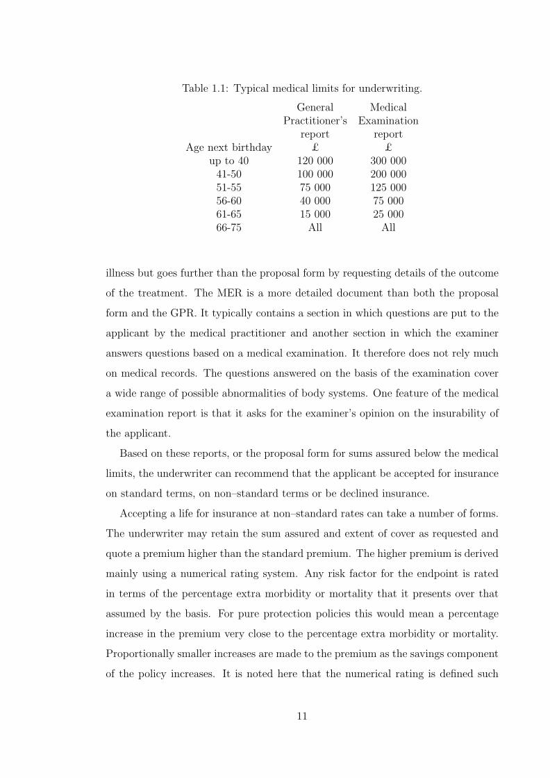
Table 1.1: Typical medical limits for underwriting.
General MedicalPractitioner’s Examination
report reportAge next birthday £ £
up to 40 120 000 300 00041-50 100 000 200 00051-55 75 000 125 00056-60 40 000 75 00061-65 15 000 25 00066-75 All All
illness but goes further than the proposal form by requesting details of the outcome
of the treatment. The MER is a more detailed document than both the proposal
form and the GPR. It typically contains a section in which questions are put to the
applicant by the medical practitioner and another section in which the examiner
answers questions based on a medical examination. It therefore does not rely much
on medical records. The questions answered on the basis of the examination cover
a wide range of possible abnormalities of body systems. One feature of the medical
examination report is that it asks for the examiner’s opinion on the insurability of
the applicant.
Based on these reports, or the proposal form for sums assured below the medical
limits, the underwriter can recommend that the applicant be accepted for insurance
on standard terms, on non–standard terms or be declined insurance.
Accepting a life for insurance at non–standard rates can take a number of forms.
The underwriter may retain the sum assured and extent of cover as requested and
quote a premium higher than the standard premium. The higher premium is derived
mainly using a numerical rating system. Any risk factor for the endpoint is rated
in terms of the percentage extra morbidity or mortality that it presents over that
assumed by the basis. For pure protection policies this would mean a percentage
increase in the premium very close to the percentage extra morbidity or mortality.
Proportionally smaller increases are made to the premium as the savings component
of the policy increases. It is noted here that the numerical rating is defined such
11
that if the premium payable by the higher risk group is, say 135% of the standard
premium, then the higher premium is expressed as a rating of +35. A rating is
only interpreted in terms of the standard (or basis) premium used to derive it. The
underwriter may also rate the policy by retaining the standard premium and extent
of cover but putting a restriction on the sum assured. The form of the restriction
on the sum assured will reflect the nature of the risk factor. If the risk factor is
temporary then a decreasing debt may be applied to the sum assured such that any
claims made after a given time will receive the standard sum assured. A third way
of rating the policy is to restrict the extent of cover by excluding claims triggered
by some specified causes.
The underwriting philosophy may aim to accept at standard rates about 75% of
the applicants with approximately 20% being accepted at non standard rates. The
remaining 5% are likely to be declined. These stated proportions are in respect of
applications for critical illness insurance (see Pokorski (1999)) and the corresponding
values for income protection insurance could be similar. For life insurance, approx-
imately 90% to 97% percent of applicants are accepted at standard rates, about
2% are accepted at non-standard rates and the remainder are declined, deferred or
reassured (Leigh (1990)).
Applicants accepted at standard rates typically include those whose premium
ratings are below +25. However we note that, from their definition, these ratings
are influenced by the definition of the standard premiums. A high standard premium
leads to a higher proportion of applicants being accepted on standard terms.
1.2 Genetics
1.2.1 Cells, chromosomes and DNA
The nucleus of each cell in the human body normally contains 23 pairs of chromo-
somes. All the cells in the body originate from one cell. The nucleus of this first cell
consists of 23 single chromosomes provided by the sperm cell and 23 single chromo-
somes provided by the egg cell from the parents. The rest of the body’s cells are
then obtained from this first one by successive cell division.
12

The chromosomes are numbered 1 to 23, numbered from the longest to the short-
est, but with chromosome 21 being shorter than chromosome 22. Those numbered
1 to 22 are called the autosomes and the 23rd is the sex chromosome. Chromosomes
are made up of DNA. Each chromosome consists of a sequence of genes, as well as
some zones which perform regulatory functions and also some other material. Sud-
bery (1998) defines a gene as a sequence of DNA that contributes to the phenotype
in a way that depends on its sequence. The term genotype refers to the physical
nature of the chromosomes in relation to the whole 23 pairs of chromosomes or to
some specific region (gene locus) or combinations of loci. The phenotype is the
expression (as an example disease status or hair colour) associated with some geno-
type. However any such expression may also be associated with another genotype
in which case it is called a phenocopy.
Apart from the DNA in the nucleus, the cell also contains DNA in the mitochon-
dria that are in the cytoplasm. This DNA is called mitochondrial DNA (mtDNA).
mtDNA is inherited from the mother and although it has not been implicated in
BCOC, CHD and stroke, it will be relevant in diseases resulting from abnormalities
in how the cell produces energy for metabolism, growth and movement from storage
molecules, and how that energy is produced for those ends.
DNA is made up of four bases: adenine (A), cytosine (C), guanine (G) and
thymine (T). The structure of genetic information is in the sequence of the bases.
The two antiparallel strands (called the ‘sense’ and the ‘antisense’ strands) are
paired such that an adenine base is always complementary to a thymine base, and
guanine is always complementary to cytosine. When two bases are joined they form
a nucleotide base pair. DNA serves a number of functions, chiefly:
(a) storing genetic information in its structured sequence,
(b) duplicating genetic information to enable it to be used for protein synthesis,
and
(c) duplicating genetic information for creating new cells.
13

1.2.2 Duplicating genetic information for protein synthesis
Gene expression is the term associated with the duplication of genetic material and
its use for protein synthesis. The sequence of the DNA codes the amino acid sequence
for protein synthesis. However protein synthesis takes place outside the nucleus and
therefore the information contained in the DNA sequence has to be transferred to
the cytoplasm for use in the protein synthesis. This is done by producing from the
DNA in the nucleus, a replica in the form of RNA. This RNA is then transported
to the cytoplasm where the information is ‘decoded’ in the protein synthesis. The
process of producing the RNA from the DNA in the nucleus is called transcription
and the process of producing the protein molecules from the RNA in the cytoplasm
is called translation. Both the transcription and translation processes have risks of
mistakes in the transfer of information. We note that the main advantage in having
the RNA carry the genetic information from the nucleus to the cytoplasm instead
of having the DNA do the transfer itself is that DNA can pass on information to
many RNA copies and therefore amplify the protein synthesis process.
1.2.3 Duplicating genetic information for creating new cells
New cells are required for body growth and for passing on genetic information to the
next generation through reproduction. Mitosis is a process in which a cell divides
into two identical cells. This involves the DNA in the nucleus being duplicated
so that a second identical nucleus is created. For producing sex cells (egg and
sperm cells) another process, called meiosis, allows the production of cells with
half the genetic information contained in non-sex cells. In each parent, the meiosis
process includes a ‘crossover’ stage when the genes from the homologous pair of one
chromosome are shuffled such that the chromosome passed on to the offspring is
not identical to any of the two chromosomes of the parent. This is important for
enhancing variation.
Meiosis or mitosis can also result in some errors. There are about 3000 million
base pairs in 23 single chromosomes in each cell (Sudbery (1998)) involved in cell
division. With approximately 1027 mitotic cell divisions occurring in an average
human lifetime (Strachan and Read (1999)) it is clear that the chances of errors
14

in the new genetic material are large. Most of the errors that actually occur are
rectified by DNA repair mechanisms but some remain. Any such mutations that
occur in the cells not involved with reproduction will be confined to that individual
but errors in the sex cells may be passed on to the offspring.
1.2.4 Mutations and disorders
The main distinction in types of errors is that some errors occur at chromosome
level while some occur at the nucleotide base level. Strachan and Read (1999) note
a number of chromosomal abnormalities, and the main ones are:
(a) the cell gaining or losing a complete chromosome,
(b) parts of chromosomes which break being re-joined to the wrong position on the
chromosome or to a different chromosome, and
(c) deletion of parts of some chromosomes.
Such abnormalities are usually so severe as to be incompatible with life or they
present a phenotype (like Down Syndrome) which may be distinct from birth. At the
nucleotide level the three main mutations are substitutions, insertions, and deletions
of single or clustered bases in the gene or chromosome.
Monogenic disorders are due to a defect in a single gene. They are classified
in three groups. Monogenic disorders are autosomal recessive if they require the
inheritance of mutations at a gene in both homologous chromosomes. Monogenic
disorders are autosomal dominant if they require the inheritance of a mutation at
a gene in only one of the homologous pair of chromosomes. In some disorders the
one mutation inherited may not cause onset but a second somatic (not inherited)
mutation at the homologous chromosome gene, or some other locus, will trigger the
onset. This is referred to as the ‘two hit’ hypothesis. Such a disorder will have
a pedigree similar to that of an autosomal dominant disorder. The third type of
single gene disorders are called X-linked because they are due to defects on the
X sex chromosome. We refer the reader to Sudbery (1998) for a fuller discussion
on the issues which make the study of single gene disorders complex. However we
point out four of them here. Firstly, the penetrance of a disorder gives a measure
of the proportion of lives who have the mutation who actually develop the disease.
15
Complete penetrance means all lives with a mutation will develop the disease and
penetrance of, say, 50% by age 60 means that half of lives born with the mutation
are expected to develop the disease before age 60. The incomplete penetrance of
some monogenic disorders will result in pedigrees that deviate from the classical
autosomal dominant or recessive pedigrees. Secondly, expressivity means that the
severity of a disorder can be different in people with similar mutations. Therefore
a monogenic disorder whose severity in one individual is so low that the disease is
not noticed will lead to a distortion of the disease pedigree. Thirdly, phenocopies
may result if environmental factors can give rise to the same disease expression as
the gene mutation. This will also distort the disease pedigrees. Fourthly, genetic
heterogeneity occurs when alleles at more than one locus can individually cause
disease onset. Examples of genetic heterogeneity include breast cancer which can
be caused by mutations at the gene loci BRCA1 or BRCA2 and adult polycystic
kidney disease which can be due to mutations at APKD1 or APKD2.
Multifactorial disorders are due to both genetic mutations and environmental
factors. Monogenic disorders with incomplete penetrance may be considered as
complex disorders. More usually the term complex or multifactorial disorders is
used in cases where there is expectation of simultaneous action of two or more genes
with or without environmental interaction. There is no clear relationship between
genotype and phenotype and multifactorial disorders do not form clear inheritance
patterns.
1.2.5 Genetic testing and insurance
The availability of genetic testing allows mutations at given loci to be investigated
in lives that do not yet have the disease. In general this will only reveal mutations
which are inherited. There are three cases of concern which we consider in turn
below.
There are disorders which are monogenic, with neither genetic heterogeneity nor
phenocopies. Lives that do not inherit the mutations will not get the disease while
lives that do so may get the disease at sometime during their lifetime, should they
live long enough. The likelihood of mutation carriers developing the disease depends
16
on the penetrance of the mutations. If the penetrance is such that the disease has
late onset, then at ages of insurance purchase, the life may not have developed
symptoms of the disease. Huntington’s disease is an example of such a disorder. We
will not consider such disorders in this work.
Most disorders are not of the type discussed above. Some monogenic disorders can
be caused by inherited mutations at two or more different loci. The disease endpoints
can also be caused by somatic mutations or by non-genetic causes. Therefore both
lives that inherit mutations and those that do not are at risk of disease. Typically
the risk is much higher for the former.
The third case for concern is that of multifactorial disorders. Lives presenting
for insurance may have genotypes associated with the disease, through pathways
yet unknown, or genotypes associated with known risk factors for the disease. The
lives, in addition, may or may not have known risk factors, possibly environmental,
which interact with the genotype.
The problem for underwriting is how to deal with any heterogeneity in the pop-
ulation introduced by the genetic information. This has to be done with particular
attention to a number of issues discussed below.
(a) The impact of heterogeneity given the type of insurance product concerned.
The heterogeneity may be more significant for critical illness products than,
say, whole life insurance products. The impact may be less on predominantly
savings products than on protection policies. Of particular importance are any
possible relations of this impact to policy conditions like the term of policy, the
sum assured, any freedom of the policyholder to increase or reduce the benefits,
and whether the purchase of insurance cover is compulsory or not.
(b) The impact of heterogeneity given the use of traditional risk classification, the
point being the adequacy of traditional ‘non-genetic’ risk classification factors
for correctly stratifying the population. Family history, usually in some limited
form, is currently used alongside a lot of medical and non-medical factors in risk
classification.
(c) Concerns of society given the impact of heterogeneity. We have seen before
how society may choose to use or not to use some classification factor. In
17

this case, careful attention may need to be paid to the arguments both for
and against genetic based risk classification. These arguments would take into
account factors like the following:
1. The consumer requirement for the insurance. Concern is more likely about
risk classification which makes health insurance in North America, say,
unaffordable to high risk groups than when CI cover is unaffordable to the
same high risk groups. Currently in the UK, it seems there is no life or
health insurance product which is viewed as vital in the same way as health
insurance in North America.
2. The proportion of the population who may be adversely affected by ge-
netic based risk classification. Most of the monogenic disorders are rare
while multifactorial disorders are common. Relatively small proportions of
society may be adversely affected by genetic risk classification for mono-
genic disorders. This may result in the rest of society being indifferent to
their fate or their small proportion making it affordable for all to absorb
the costs of insuring these high risk groups. The situation may be differ-
ent for common disorders. The proportion of the population affected may
be sufficiently large that the remainder may not be willing to subsidize
the costs. However, it may not be desirable that such a big proportion of
society is left to meet their own higher costs of insurance.
Within this context, the A.B.I. genetics committee in December 1997 published
the industry’s voluntary code of practice (A.B.I. (1997)). The code detailed proce-
dures to be followed by insurance companies on the use of, and handling of, genetic
information. Among the principles set out in the code is that the insurers would
only use genetic test results that the applicant already had, and therefore would not
ask for tests to be done specifically for assessing the insurance application. In the
case where these test results were available, their use in the assessment for insur-
ance was restricted to cases where ‘their reliability and relevance to insurance’ was
established. They also set that applicants should not be offered lower than standard
18
premiums on the basis of negative genetic test results. The H.G.A.C. also pub-
lished a report in December 1997 on the implications of genetic testing for insurance
(H.G.A.C. (1997)). The report also recommended that for a genetic test to be used
for assessment of insurance applications, a quantifiable association between the test
results and insurance costs should be established. They further recommended that
the government should set up an independent body to assess evidence for associa-
tions between various genetic tests and insurance costs. The Genetics and Insurance
Committee (G.A.I.C.) was set up for this purpose and the A.B.I. set out to submit
evidence for tests for mutations associated with seven disorders to be accepted as
reliable and relevant by the G.A.I.C. The A.B.I. set out to submit evidence in re-
lation to the disorders Huntington’s disease, myotonic distrophy, familial polyposis,
multiple endocrine neoplasia, early-onset Alzheimer’s disease, hereditary breast and
ovarian cancer and hereditary motor and sensory neuropathy. In 2000 G.A.I.C. ap-
proved the use of the genetic test results for Huntington’s disease with respect to life
insurance. In November 2000 the Human Genetics Commission (H.G.C.), a body
which advises government, launched a discussion document on the storage protec-
tion and use of personal genetic information titled ‘Whose hands on your genes’.
The document invited from the general public responses to questions on whether
insurers should be able to ask for genetic test results for underwriting and if so
whether there should be controls on the way the information is used. Views were
also invited on whether the type of insurance, type of genetic condition or level of
sum assured should affect the decision to use genetic information. In March 2001
the House of Commons Science and Technology select committee issued a report
in which they criticised the insurance industry’s lack of consistency with respect
to interpretation of, and compliance with, the voluntary code of conduct. The se-
lect committee report said that it was wrong for insurance companies to be using
genetic test results for underwriting when their relevance had not been verified by
the G.A.I.C. In response to the select committee report, and to some extent the re-
sponses to its discussion document, in May 2001 the H.G.C. published a document
suggesting that a moratorium of no less than three years be put in place on the use
19
of genetic tests information by insurance companies. Shortly after, the A.B.I. an-
nounced an agreement it reached with the government to effect a 5 year moratorium
on the use of genetic test results except in the cases of very high sum assured and
in those cases using only the tests approved by G.A.I.C.
This work seeks to contribute to the task of assessing the relevance of genetic
test results to insurance costs. For the monogenic disorders of breast cancer and
ovarian cancer we aim to quantify the effect of heterogeneity due to mutations at two
gene loci, BRCA1 and BRCA2, with respect to CI policies. For the multifactorial
cardiovascular disorders, this work aims to contribute by producing a model that
can be used to quantify the effect of heterogeneity due to mutations that may be
identified in future. The difficulty of proceeding beyond a general model to assess
the implications of specific loci is due to the lack of comprehensive genetics on
cardiovascular disorders to date. On this problem, the H.G.A.C. wrote the following
in their 1997 report (H.G.A.C. (1997)),
“We conclude that it is unlikely that actuarially important genetic predictions of
common causes of adult death will be available and validated, for some time to come.
This is because the information linking genetics and multifactorial disease is at too
early a stage to make sound assessment of added risk.”
To quantify the impact of genetic test results on insurance costs, Macdonald
(1997) suggested the use of multiple state Markov models which capture levels of
genetic testing in the population, the insurance purchase behaviour of lives with
different genotypes, and the underwriting decisions for types of insurance policies.
Markov models and the model of heterogeneity are discussed next, in Section 1.3.
1.3 Continuous time Markov models
We will use various multiple state models in continuous time. In a multiple state
model, we can completely specify a model by the states and the transition intensities
between the states. We refer the reader to Waters (1984) who gives a good discus-
sion of multiple state models and the advantages of specifying a model in terms of
transition intensities.
20
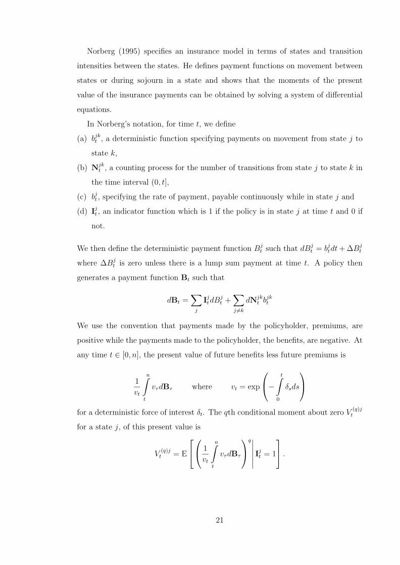
Norberg (1995) specifies an insurance model in terms of states and transition
intensities between the states. He defines payment functions on movement between
states or during sojourn in a state and shows that the moments of the present
value of the insurance payments can be obtained by solving a system of differential
equations.
In Norberg’s notation, for time t, we define
(a) bjkt , a deterministic function specifying payments on movement from state j to
state k,
(b) Njkt , a counting process for the number of transitions from state j to state k in
the time interval (0, t],
(c) bjt , specifying the rate of payment, payable continuously while in state j and
(d) Ijt , an indicator function which is 1 if the policy is in state j at time t and 0 if
not.
We then define the deterministic payment function Bjt such that dBj
t = bjtdt + ∆Bj
t
where ∆Bjt is zero unless there is a lump sum payment at time t. A policy then
generates a payment function Bt such that
dBt =∑
j
IjtdBj
t +∑j 6=k
dNjkt bjk
t
We use the convention that payments made by the policyholder, premiums, are
positive while the payments made to the policyholder, the benefits, are negative. At
any time t ∈ [0, n], the present value of future benefits less future premiums is
1
vt
n∫t
vτdBτ where vt = exp
−
t∫0
δsds
for a deterministic force of interest δt. The qth conditional moment about zero V(q)jt
for a state j, of this present value is
V(q)jt = E
1
vt
n∫t
vτdBτ
q∣∣∣∣∣∣ Ijt = 1
.
21

Norberg (1995) assumes that δt, bjkt , bj
t , and the transition intensities µjkt are piece-
wise continuous and by defining
µj·t =
∑k 6=j
µjkt ,
shows that V(q)jt is a solution of the differential equation
d
dtV
(q)jt = (qδt + µj·
t )V(q)jt − qbj
tV(q−1)jt −
∑k 6=j
µjkt
q∑r=0
(q
r
)(bjk
t )rV(q−r)kt (1.1)
with the boundary conditions V(q)jn = 0. A special case of the solution is that for
q = 1. The solution in this cases gives Thiele’s equations
d
dtV
(1)jt = δtV
(1)jt − bj
t −∑k 6=j
(bjkt + V
(1)kt − V
(1)jt )µjk
t . (1.2)
Macdonald (1997) proposes the use of Markov models which define insurance
products using the multiple state models as in Norberg (1995) but also including
the behaviour of insurance buying and insurance company underwriting behaviour
in the states and the transition intensities. Figure 1.1 shows the model used for
a homogeneous subpopulation by Macdonald (1997). We note that in figure 1.1
‘State 2’ (Not tested positive, Insured) includes lives that have tested negative and
subsequently bought insurance and those that have bought insurance without ever
taking a genetic test. By using similar models for different subpopulations (and
therefore different values of the intensities µjkx+t), he was able to assess the relative
values of insurance costs between subpopulations.
Using the approach of Macdonald (1997) will enable us to calculate the moments
of present values of insurance products under various assumptions of
(a) heterogeneity in populations,
(b) various underwriting strategies to deal with this heterogeneity,
(c) levels of genetic testing and
(d) levels of adverse selection.
22

-¾
?
SS
SSw
¶¶
¶¶/
³³³³³³³³³³³³³)
PPPPPPPPPPPPPq
SS
SSw
¶¶
¶¶/
³³³³³³³³³³³³³)
State 0
State 2 State 1 State 3 State 4
State 5
Not Tested
Not Insured
Not Tested +ve
Insured
Tested -ve
Not Insured
Tested +ve
Not Insured
Tested +ve
Insured
Dead
µ01x+t
µ03x+t
µ34x+tµ12
x+t
µ45x+tµ25
x+t
µ02x+t
µ15x+t µ35
x+tµ05x+t
Figure 1.1: Macdonald’s (1997) Markov model for insurance in the presence ofgenetic testing, insurance buying and underwriting.
We note that the transition intensities between states are a very important part
of the model specification. We will use various actuarial, medical, genetic and epi-
demiological literature sources to derive the intensities for our models. We describe,
in the next section, the nature of measures available in the literature and how we
can derive transition intensities from them.
1.4 Epidemiological statistics
In this thesis we use results from a number of different medical, genetic and epidemi-
ological studies. We also do our own statistical analysis on some data sets collected
for medical and epidemiological purposes. Here we present the statistical theory of
the various measures we use from published studies as well as those we use to derive
our required measures from available data sets.
Epidemiological studies are mainly observational studies as opposed to experi-
mental studies. Experimental studies are investigations where the researcher has
some control over some factors in the study. Observational studies draw conclusions
from observation of the subjects of study without controlling factors. We do not dis-
cuss experimental studies any further since we do not use results from such studies.
23

Observational studies fall into broad groups as follows:
(a) Longitudinal studies; also known as cohort studies. They observe a selected
population prospectively over some time period and monitor events of interest.
(b) Cross-sectional studies; such studies consider the characteristics of a selected
population at a fixed point in time.
(c) Case-control; in case-control studies, use is made of retrospective information
collected at a point in time.
1.4.1 Longitudinal studies
We consider two possible states for members of a population. These can be ‘healthy’
or ‘ill’, ‘alive’ or ‘dead’ or some other states. Of main interest are two types of
measures:
(a) the absolute rate of movement from one state to the other, and
(b) how such rates of movement compare in two related populations.
We consider these in turn.
Absolute intensities
The ‘alive’ or ‘dead’ states example can be represented by the simple two state
continuous time Markov model shown in Figure 1.2.
State AAlive
State DDead
λx+t -
Figure 1.2: Representation of the two-state Markov model.
Being Markov, the rate λx+t depends on the current state occupied by the life at
age x + t (and not on any previous life history) and on the age x + t. λx is defined
24

such that within a very short time interval, δt, of exact age x the probability of
dying is approximately proportional to δt × λx. Formally δtpADx = δt × λx + o(δt)
where a function f(t) is o(t) if
limt→ 0+
f(t)
t= 0.
λx+t is called the force of mortality. If the decrement was illness then λx+t would
be a force of morbidity. We refer to them as the transition intensities. Macdonald
(1996a) has shown that if we specify a model as above we can state
(a) the probability of remaining in State A, denoted tpAAx , is given by
tpAAx = exp
−
t∫0
λx+sds
,
and
(b) the probability of moving from State A to State D between ages x and x + t is
tpADx = 1− exp
−
t∫0
λx+sds
.
In general, expressions for probabilities of the type of tpAAx and tp
ADx (called
occupancy probabilities), are obtained by considering the Kolmogorov differential
equations. The probability tpAAx given above is a solution to the Kolmogorov equa-
tion
d
dttp
AAx = −tp
AAx (λx+t)
which satisfies the boundary condition 0pAAx = 1. If we consider a general multiple
state model with transition intensities µghx+t of moving from state g to state h, the
Kolmogorov equations are given by
d
dttp
ghx =
∑j 6=h
(tp
gjx µjh
x+t − tpghx µhj
x+t
)for g 6= h.
If the transition intensities are known, the occupancy probabilities, tpghx , can be eval-
uated by numerically solving the Kolmogorov equations subject to some boundary
conditions.
25

Considering further our example of the two state model, Macdonald (1996a) shows
that for estimation if we assume that λx+t takes a constant value λ for 0 ≤ t < 1,
the maximum likelihood estimate of λ is
λ =d
v
where d and v are the observed values of a pair of random variables D (total number
of deaths or other decrements) and V (total waiting time) based on a sample drawn
from the distribution of (D, V). If we have N statistically independent and identical
lives, then
D =N∑
i=1
Di and V =N∑
i=1
Vi
where Di is the random variable denoting the number of transitions from the alive
state to the dead state for life i, and the random variable Vi denotes the waiting
time for that life. Observational plans can be devised to allow this estimate to be
computed. It requires evaluating the number of deaths for the sample and the central
exposed to risk. Estimates of intensities such as the one above can be derived for
any general multiple state Markov model and Macdonald (1996a) gives a discussion
of this.
If the central exposed to risk can not be calculated exactly as the sum of the
observed waiting times due to observational plan limitations the census method
approximation may be used. This uses numerical integration and the numbers of
lives observed at fixed points during the observation period (the census values) to
estimate the central exposed to risk.
Concerning measures of disease occurrence, Breslow and Day (1980) note that
the incidence rate is estimated by the number of occurrences during a specified time
interval divided by the total amount of observation time accumulated during that
interval. The time interval is normally one year and the incidence rate is expressed as
the incidence per 1000 person-years of observation. If an infinitesimal time interval
is assumed then the incidence rate is defined as the hazard rate. This is equivalent
to the transition intensity as given by λx+t.
A related measure often quoted in genetic studies is the lifetime or cumulative
risk. This is the probability of occurrence of an event within a lifetime (usually up
26

to 70 or 80 years of age) starting from a given age. The lifetime risk of onset of a
disease by age x is therefore
= 1− exp
−
x∫0
λsds
for starting age 0. The integral Λx =x∫0
λsds is the integrated hazard.
In the evaluation of the total time spent under observation (the exposed to risk),
studies based on national data use the estimated population in the country. How-
ever, only lives who are at risk should contribute to the total exposure. As an
example only women should contribute to the exposure for a disease like ovarian
cancer. As another example, Breslow and Day (1980) note that for countries with
high hysterectomy rates, one should adjust the population figures for women when
considering exposure for the purpose of estimating endometrial cancer incidence.
These are special examples of how the principle of correspondence should apply to
the lives contributing to the events and to those contributing to the waiting time.
Relative risk
Studies may be done with the aim of comparing how the incidence rate compares
between two populations which differ in respect of some covariate. This is important
in the search for causes and risk factors for disease. Relative risks are also useful in
determining the absolute incidence rates in subpopulations if we know the incidence
rate in the aggregate population.
Suppose we have two identical populations P1 and P2 except that lives in P1
have a risk factor which is not present in lives of P2. The relative risk (RR)x+t of
the disease for P1 in relation to P2 is defined as the ratio,
RRx+t =λ
(P1)x+t
λ(P2)x+t
of the transition intensities. The relative risk can therefore be calculated from
the forces estimated in the manner discussed before. In most practical cases the
populations under study are not identical in respect of risk factors that influence the
transitions intensities. The Cox proportional hazards model is one of several possible
27

models used in prospective studies to estimate the relative risk in the presence of
many covariates. A discussion of the Cox model and model fitting is given by
Macdonald (1996b). The relative risk obtained from the simultaneous modelling of
many covariates is often referred to as the adjusted relative risk. This indicates that
the relative risk is adjusted for differences in the risk of disease due the differences
in the other risk factors which are not under consideration.
If we further suppose we know the absolute intensity λx+t for an aggregate pop-
ulation in which lives from P1 form a proportion px+t and the rest is made up of
lives from P2, we can write
λx+t = px+t × λ(P1)x+t + (1− px+t)× λ
(P2)x+t
and therefore
λ(P1)x+t =
RRx+t × λx+t
1 + px+t ×RRx+t − px+t
and λ(P2)x+t =
λx+t
1 + px+t ×RRx+t − px+t
using the relative risk RRx+t.
The proportion px+t, and even the relative risk RRx+t are often assumed to be
constants over the whole age range or over some parts of it.
Odds ratio
Another measure used in the medical literature to represent the relationship between
the intensities between different populations is the odds ratio. It is defined in terms
of probabilities of the event in a fixed period of time. Using the two populations P1
and P2 as before, we define p(P1) and p(P2) as the probability of an event occurring
in populations P1 and P2, respectively, in one time interval. The odds for the event
happening in P1 and P2 are p(P1)
1−p(P1) and p(P2)
1−p(P2) respectively. The odds ratio (OR)
for P1 in relation to P2 is
OR =
p(P1)
1−p(P1)
p(P2)
1−p(P2)
.
28
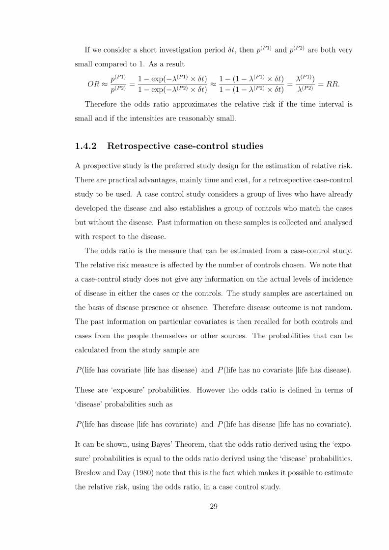
If we consider a short investigation period δt, then p(P1) and p(P2) are both very
small compared to 1. As a result
OR ≈ p(P1)
p(P2)=
1− exp(−λ(P1) × δt)
1− exp(−λ(P2) × δt)≈ 1− (1− λ(P1) × δt)
1− (1− λ(P2) × δt)=
λ(P1))
λ(P2)= RR.
Therefore the odds ratio approximates the relative risk if the time interval is
small and if the intensities are reasonably small.
1.4.2 Retrospective case-control studies
A prospective study is the preferred study design for the estimation of relative risk.
There are practical advantages, mainly time and cost, for a retrospective case-control
study to be used. A case control study considers a group of lives who have already
developed the disease and also establishes a group of controls who match the cases
but without the disease. Past information on these samples is collected and analysed
with respect to the disease.
The odds ratio is the measure that can be estimated from a case-control study.
The relative risk measure is affected by the number of controls chosen. We note that
a case-control study does not give any information on the actual levels of incidence
of disease in either the cases or the controls. The study samples are ascertained on
the basis of disease presence or absence. Therefore disease outcome is not random.
The past information on particular covariates is then recalled for both controls and
cases from the people themselves or other sources. The probabilities that can be
calculated from the study sample are
P (life has covariate |life has disease) and P (life has no covariate |life has disease).
These are ‘exposure’ probabilities. However the odds ratio is defined in terms of
‘disease’ probabilities such as
P (life has disease |life has covariate) and P (life has disease |life has no covariate).
It can be shown, using Bayes’ Theorem, that the odds ratio derived using the ‘expo-
sure’ probabilities is equal to the odds ratio derived using the ‘disease’ probabilities.
Breslow and Day (1980) note that this is the fact which makes it possible to estimate
the relative risk, using the odds ratio, in a case control study.
29

In a study with many covariates, regression models like the logistic regression or
Poisson model are used to estimate the odds ratio. The simultaneous consideration
of covariates enables the odds ratio for a particular covariate to be adjusted for all
the other covariates in the same model. Otherwise samples will need to be stratified
to levels where no confounding covariates are present. Breslow and Day (1980) give
a discussion of these regression methods.
1.4.3 Cross-sectional studies
Cross-sectional studies give a snapshot picture of the covariates and disease profile of
a surveyed population. The data collected from such a study are ideal for estimating
the point prevalence of a disease. The point prevalence is the proportion of the
population who have the disease at the point of investigation. The point prevalence
or proportion described above can be used in estimating absolute incidence rates in
subpopulations given the aggregated population incidence rates and the RR.
It is important, in the use of prevalence estimates from cross-sectional studies,
to ensure that the sample on which the estimates are based is representative (in
respect of the relevant attributes) of the population to which they may be applied.
The proportion, the relative risk or the odds ratio, can vary by factors like age and
sex which may be of interest. Some large studies will give these measures estimated
for the different levels of the factors. However many studies may report only an
aggregate value of any particular measure.
1.5 Critical illness insurance
Critical Illness (CI) or Dread Disease cover is insurance in which a claim is triggered
by the diagnosis of some specified disease or the performance of some specified
medical procedure. In the United Kingdom, most CI policies cover the illnesses
listed below.
(a) cancer,
(b) heart attack,
(c) stroke,
30

(d) coronary artery bypass,
(e) major organ transplant,
(f) chronic kidney failure,
(g) multiple sclerosis, and
(h) total permanent disability.
In addition there are more than 30 other conditions covered under CI insurance
policies by different insurance companies. There is consumer need for insurance
policies that give some benefit related to the onset of these illnesses. This is due
to the fact that the illnesses may require treatment which can be very expensive or
take a long period of time so as to cause the patient loss of income. Benefits may
be needed to pay for treatment, pay for nursing care, pay off a mortgage, or just
to make the difficult time of illness more bearable. CI policies partly meet these
requirements by paying a lump sum on diagnosis. The nature of benefits differ with
the type of CI policy and these types fall into three main groups.
(a) Stand-alone CI Insurance Policies: The full sum assured is paid out on proof of
diagnosis of any of the covered diseases. Stand-alone policies constituted about
14% of all new CI insurance policies sold in the UK in 1998 and about 15% of
all CI insurance policies in force at end of 1998 (see Dinani et al. (2000)). The
insured has to survive a period of between 14 and 90 days after diagnosis for the
claim to be paid out. The typical survival period is 28 days as used by Dinani
et al. (2000). The policies normally have a three month waiting period in which
claims can not be made.
(b) Accelerated Benefit: In this type of CI insurance policy the benefit is paid as an
acceleration of another benefit (like a death benefit) on the diagnosis of a covered
disease. This acceleration will be 100% if it pays out the whole sum assured on
diagnosis. Otherwise it will be a partial acceleration. For a 100% acceleration,
if the policyholder gets the sum assured on diagnosis of a disease, the policy is
no longer in force and on death they will not get any more payment. In the case
of partial acceleration, the death of the policyholder means the balance of the
sum assured will be paid to the beneficiary. Accelerated benefit CI insurance
policies formed 86% of all new CI insurance policies sold in the UK in 1998 and
31
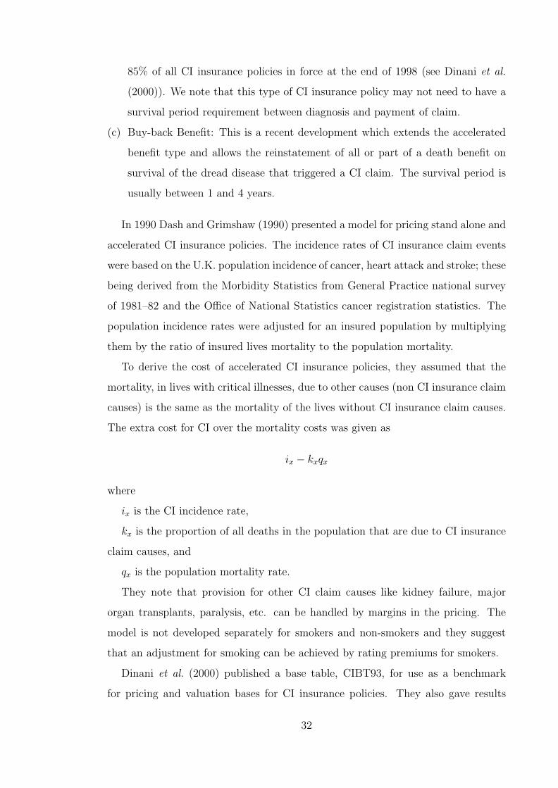
85% of all CI insurance policies in force at the end of 1998 (see Dinani et al.
(2000)). We note that this type of CI insurance policy may not need to have a
survival period requirement between diagnosis and payment of claim.
(c) Buy-back Benefit: This is a recent development which extends the accelerated
benefit type and allows the reinstatement of all or part of a death benefit on
survival of the dread disease that triggered a CI claim. The survival period is
usually between 1 and 4 years.
In 1990 Dash and Grimshaw (1990) presented a model for pricing stand alone and
accelerated CI insurance policies. The incidence rates of CI insurance claim events
were based on the U.K. population incidence of cancer, heart attack and stroke; these
being derived from the Morbidity Statistics from General Practice national survey
of 1981–82 and the Office of National Statistics cancer registration statistics. The
population incidence rates were adjusted for an insured population by multiplying
them by the ratio of insured lives mortality to the population mortality.
To derive the cost of accelerated CI insurance policies, they assumed that the
mortality, in lives with critical illnesses, due to other causes (non CI insurance claim
causes) is the same as the mortality of the lives without CI insurance claim causes.
The extra cost for CI over the mortality costs was given as
ix − kxqx
where
ix is the CI incidence rate,
kx is the proportion of all deaths in the population that are due to CI insurance
claim causes, and
qx is the population mortality rate.
They note that provision for other CI claim causes like kidney failure, major
organ transplants, paralysis, etc. can be handled by margins in the pricing. The
model is not developed separately for smokers and non-smokers and they suggest
that an adjustment for smoking can be achieved by rating premiums for smokers.
Dinani et al. (2000) published a base table, CIBT93, for use as a benchmark
for pricing and valuation bases for CI insurance policies. They also gave results
32

of the CI insurance claims experience investigations for the period 1991 to 1997.
The base table gives the incidence rates for a stand alone CI policy as a sum of
the incidence rates of cancer, heart attack, stroke, coronary artery bypass grafting,
multiple sclerosis, kidney failure, multiple organ transplant and total permanent
disability. The incidence rates for various illnesses are derived from U.K. population
data like the O.N.S. cancer registrations, Morbidity Statistics from General Practice
1991–92 survey, the Oxford Community Stroke Project and others. The population
incidence rates were adjusted as follows:
(a) First-ever adjustment; to remove influence of recurrent episodes of illnesses.
(b) Sudden death adjustment; to include the influence of cases that will be unre-
ported due to sudden death.
(c) Overlap with other CI; to remove double counting that may occur due to dif-
ferent illness occurring to the same individual.
(d) Prevalence adjustment; to reduce the influence of the fact that the denominator
used in calculation the incidence rates is the total population of the U.K. when
it should be the disease free population.
(e) 28–day survival adjustment; to remove the proportion of lives who develop CI
but do not survive the 28 days required for a claim to be valid.
Provision is made for the incidence of other CI insurance claim causes like Parkin-
son’s disease, angioplasty, terminal illness and others. Their incidence rate is ex-
pressed as a percentage of the incidence rate of the base table. The total percentage
of these ‘other causes’ ranges from 5% for males (3.5% for females) at ages 20 to 24
to 25% for males (35% for females) at ages 75 to 80.
For accelerated policies the incidence rates were based on the Dash and Grimshaw
(1990) model. The proportion kx was derived from the O.P.C.S. ‘Mortality by Cause’
publications.
33

Chapter 2
Genetic and family history models
for breast and ovarian cancer
2.1 Breast cancer
Breast cancer (BC) forms one of the biggest proportions of cancers suffered by
women. Of about 280,000 new cases of cancers recorded in females in the U.K.
between 1990 and 1992, approximately 92,000 were BC cases (O.N.S. (1999)). This
represents about a third of all new cancer cases. Souhami and Tobias (1998) note
that the prevalence is such that about one-half of all live female cancer patients are
suffering from BC.
The diagnosis of BC is mainly made by the withdrawal of fluid from the body for
examination (aspiration), the withdrawal of tissue (biopsy) or by an X-ray exami-
nation called a mammogram. Various treatment regimes are used at present. These
include surgery, radiotherapy, hormonal manipulation and chemotherapy. Souhami
and Tobias (1998) note that part of the investigation that is done before treatment is
started is aimed at excluding patients whose cancer has spread so much that they are
unlikely to benefit from treatment. To aid in such an assessment there are staging
systems to grade the cancers. The Manchester staging system given in Table 2.2 is
one such staging criterion. We note that such staging is only to distinguish cancers
by advancement at time of diagnosis. They do not represent different cancers.
34

Table 2.2: Manchester staging system given in Souhami and Tobias (1998).
Stage Description
Stage I Breast alone involved with or without overlying skin.Stage II Breast as for stage I and axillary nodes involved,
but mobile.Stage III Skin invaded, fixed or ulcerated, or tumour
fixed to underlying muscle or pectoral fascia.Stage IV Fixed axillary lymphadenopathy, superclavicular
involvement and/or distant metastases.
In all cases one of three prognoses is possible for patients under treatment. A
patient can survive the particular episode, after treatment, without recurrence of
BC. They can also survive the particular episode but with a recurrence of BC at a
later time or at some later time the patient dies, before recovering from this episode,
from BC (or other causes). Those who survive are also still at risk of developing
other cancers, alongside any other illness.
In the U.S.A. an average of 85.1% of patients diagnosed with BC between 1990
and 1992 survived for five years after diagnosis (Ries et al. (2000)). In the U.K
72% of women whose BC was diagnosed between 1986 and 1990 survived for five
years after diagnosis (Coleman et al. (1999)). Survival chances are higher for those
whose tumours are discovered before they spread. According to Souhami and Tobias
(1998), five-year survival times for Stage I diagnoses are about three times those of
Stage II diagnoses. This underlies the efforts to achieve early diagnosis of BC. The
UK introduced systematic BC screening in 1988 for all women aged 50 to 64 with
three–year intervals between screenings.
BC is a major cause of death in women. Of the deaths registered between 1990
and 1992 in England and Wales, BC was the cause of 5% of them in women between
the ages of 50 and 90 (O.P.C.S. (1991b), O.P.C.S. (1993b) and O.P.C.S. (1993c)).
There are a number of factors which are established to be associated with in-
creased risk of BC. The following are given by Spicer and Pike (1999);
(a) increasing age,
(b) early menarche,
35

(c) late menopause,
(d) proliferative breast disease,
(e) family history of early onset, bilateral disease, or multiple first degree relatives
affected,
(f) BRCA1 or BRCA2 mutations,
(g) postmenopausal obesity,
(h) late first term pregnancy or nulliparity,
(i) race, North American or Western European,
(j) mammographic pattern of greater density, and
(k) ionizing radiation exposure.
For diseases affecting women only, first degree relatives refer to the mother and
full sisters (otherwise it includes the father and full brothers as well). Spicer and
Pike (1999) discuss these risk factors in greater detail and we will consider some of
them in later sections. However it is important to note that even though there are
many risk factors, Etkind and Sparano (1999) state that almost one half of all BC
patients have no identifiable risk factor.
The underwriting for CI policies will be considered. We will discuss the current
underwriting in terms of BC risk factors to enable us to assess the impact of genetic
risk factors. The BC genetic risk factors, BRCA1 and BRCA2, are also risk factors
for ovarian cancer (OC) and so we will consider breast cancer and ovarian cancer
(BCOC) together in our modelling. The next section discusses the characteristics
of OC.
2.2 Ovarian cancer
In the U.K, between 1990 and 1992 there were about 15,800 new cases of OC (O.N.S.
(1999)), which is 5.6% of all new cancer cases in women. The symptoms associated
with OC include gross swelling of the abdomen, vomiting, change in bowel function
and urinary frequency. A number of tests are used for diagnosis of OC. These include
physical examination, computerised tomography and magnetic resonance imaging,
X-rays, intravenous pyelogram, transvaginal sonography, serum CA 125 checks and
36

cytologic examinations. Chi and Hoskins (1996) note that there are differences in
the sensitivity ( getting positive test results in people with the disease ) and the
specificity ( getting negative test results in people without the disease ) and discuss
the situations in which they should be applied. However, as Souhami and Tobias
(1998) discuss, early ovarian cancer is largely asymptomatic and the early symptoms
are usually vague and non-specific. This means that most OC diagnoses are made
when the tumour has spread. The treatment methods used for OC patients include
surgery, radiotherapy and chemotherapy.
An average of 51% of OC patients in the USA, diagnosed between 1990 and 1992,
survived for at least five years after diagnosis (Ries et al. (2000)). In the U.K. of
those OC patients diagnosed between 1986 and 1990, 29% survived for five years
after diagnosis (Coleman et al. (1999)). Survival times depend a lot on the extent
of the disease spread at the time of diagnosis.
U.K mortality by cause statistics, O.P.C.S. (1991b), O.P.C.S. (1993b) and
O.P.C.S. (1993c), show that between 1990 and 1992 11,705 deaths due to OC were
recorded in England and Wales. This is about 1.4% of all deaths recorded in women
in the same period.
Methods and completeness of registrations of cancers in countries have significant
influence on incidence and survival rates and the results of any comparisons made
between countries.
Factors associated with an increased risk of ovarian cancer include;
(a) increasing age,
(b) nulliparity,
(c) infertility,
(d) late age at menopause,
(e) history of breast cancer,
(f) mutations at BRCA1, BRCA2, MSH2, MLH1, PMS1, and PMS2 genes, and
(g) a family history of breast and/or ovarian cancer.
Parazzini et al. (1991) and Gajewski and Legare (1998) discuss these and other
factors. We will discuss the genetic risk factors as well as family history later in the
chapter.
37
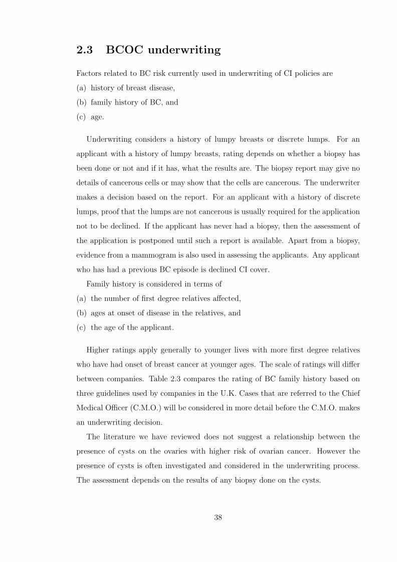
2.3 BCOC underwriting
Factors related to BC risk currently used in underwriting of CI policies are
(a) history of breast disease,
(b) family history of BC, and
(c) age.
Underwriting considers a history of lumpy breasts or discrete lumps. For an
applicant with a history of lumpy breasts, rating depends on whether a biopsy has
been done or not and if it has, what the results are. The biopsy report may give no
details of cancerous cells or may show that the cells are cancerous. The underwriter
makes a decision based on the report. For an applicant with a history of discrete
lumps, proof that the lumps are not cancerous is usually required for the application
not to be declined. If the applicant has never had a biopsy, then the assessment of
the application is postponed until such a report is available. Apart from a biopsy,
evidence from a mammogram is also used in assessing the applicants. Any applicant
who has had a previous BC episode is declined CI cover.
Family history is considered in terms of
(a) the number of first degree relatives affected,
(b) ages at onset of disease in the relatives, and
(c) the age of the applicant.
Higher ratings apply generally to younger lives with more first degree relatives
who have had onset of breast cancer at younger ages. The scale of ratings will differ
between companies. Table 2.3 compares the rating of BC family history based on
three guidelines used by companies in the U.K. Cases that are referred to the Chief
Medical Officer (C.M.O.) will be considered in more detail before the C.M.O. makes
an underwriting decision.
The literature we have reviewed does not suggest a relationship between the
presence of cysts on the ovaries with higher risk of ovarian cancer. However the
presence of cysts is often investigated and considered in the underwriting process.
The assessment depends on the results of any biopsy done on the cysts.
38
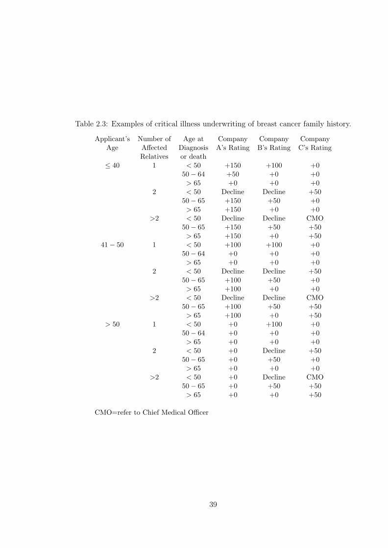
Table 2.3: Examples of critical illness underwriting of breast cancer family history.
Applicant’s Number of Age at Company Company CompanyAge Affected Diagnosis A’s Rating B’s Rating C’s Rating
Relatives or death≤ 40 1 < 50 +150 +100 +0
50− 64 +50 +0 +0> 65 +0 +0 +0
2 < 50 Decline Decline +5050− 65 +150 +50 +0> 65 +150 +0 +0
>2 < 50 Decline Decline CMO50− 65 +150 +50 +50> 65 +150 +0 +50
41− 50 1 < 50 +100 +100 +050− 64 +0 +0 +0> 65 +0 +0 +0
2 < 50 Decline Decline +5050− 65 +100 +50 +0> 65 +100 +0 +0
>2 < 50 Decline Decline CMO50− 65 +100 +50 +50> 65 +100 +0 +50
> 50 1 < 50 +0 +100 +050− 64 +0 +0 +0> 65 +0 +0 +0
2 < 50 +0 Decline +5050− 65 +0 +50 +0> 65 +0 +0 +0
>2 < 50 +0 Decline CMO50− 65 +0 +50 +50> 65 +0 +0 +50
CMO=refer to Chief Medical Officer
39

Table 2.4: Examples of critical illness underwriting of ovarian cancer family history.
Applicant’s Number of Age at Company CompanyAge Affected Diagnosis A’s Rating B’s Rating
Relatives or death≤ 40 1 < 50 +100 +150
50− 64 +50 +50> 65 +0 +0
> 2 < 50 +150 Decline50− 65 +75 +150> 65 +25 +150
41− 50 1 < 50 +100 +10050− 64 +50 +0> 65 +0 +0
> 2 < 50 +150 Decline50− 65 +75 +0> 65 +25 +0
> 50 Any Any +0 +0
Table 2.4 shows examples of CI policy underwriting in the presence of OC family
history.
The ratings used by particular companies will reflect the morbidity bases under-
lying the policies they are selling. The ratings are therefore bound to be different
especially as the morbidity basis used by a company may be based, to some ex-
tent, on the company’s own morbidity experience. However a common factor in CI
underwriting based on family history of BC is that it does not routinely take into
account
(a) the total number of first degree relatives,
(b) ages of first degree relatives not affected by BC,
(c) the actual nature of the relationship between the applicant and the first degree
relatives who have had BC or OC, and
(d) information on other (second degree) female relatives, like maternal and paternal
aunts.
The information for (a) , (b) and (c) is usually collected on the proposal form
completed by the applicant while information on other relatives is not normally
collected.
40

2.4 Genetics of breast cancer and ovarian cancer
2.4.1 BRCA1 and BRCA2 susceptibility genes
Analysis of the occurrence of breast cancer in some large families showed that the
number of cancer cases in the families were much higher than what could be at-
tributed to chance or other known risk factors. This led to studies aimed at estab-
lishing the hereditary link between the cancers in these families. Claus et al. (1991)
observed that the risk of BC was much higher in women with two or more first
degree relatives with BC than women with fewer than two relatives with BC. This
supported the hypothesis that the distribution of BC in the general population in-
cluded a small number of genetic cases combined with a larger number of non-genetic
cases. Most studies found that the transmission of BC in families was explained best
by a genetic model in which a locus has an autosomal dominant mode of inheritance
(Claus et al. (1991)). The Cancer and Steroid Hormone (C.A.S.H.) study, reported
by Claus et al. (1991), is one of the most important of these studies. It is based on
a case-control study of 4,703 BC cases and its main results are summarised below.
(a) The transmission of BC is best fitted by the existence of a diallelic locus with
an autosomal dominant mode of transmission.
(b) The frequency of the high risk allele is 0.0033.
(c) If the age at onset of BC is represented by a step function, then the cumulative
probability of BC by genotype is as given in Table 2.5.
Table 2.5: Cumulative probabilities of BC under the C.A.S.H. model. (Source:Claus et al. (1991).)
Cumulative probability of BC by age;Genotype 20–29 30–39 40–49 50–59 60–69 70–79 80+Aa/AA 0.0167 0.1444 0.3758 0.5477 0.6743 0.9452 1
aa 0.0002 0.0027 0.0138 0.0275 0.0497 0.0798 0.1254Ratio 83.5 53.5 27.2 19.9 13.6 11.8 8.0
(d) The ratio of the hazard function for individuals with different genotypes is not
constant but depends on age.
41

Table 2.6: Cumulative probabilities of BC for a woman with one first degree relativewith BC (under the C.A.S.H. model). (Source: Claus et al. (1994).)
Age of Age at onset of BC in relativewoman 20–29 30–39 40–49 50–59 60–69 70–79
29 0.007 0.005 0.003 0.002 0.002 0.00139 0.025 0.017 0.012 0.008 0.006 0.00549 0.062 0.044 0.032 0.023 0.018 0.01559 0.116 0.086 0.064 0.049 0.040 0.03569 0.171 0.130 0.101 0.082 0.070 0.06279 0.211 0.165 0.132 0.110 0.096 0.088
Claus et al. (1994) produced tables for use in risk prediction for women with a
family history of BC. These were based on the C.A.S.H. model and Table 2.6 shows
one of these tables relating to a family history of one first-degree relative with BC.
They gave other tables which consider a family history of two first degree relatives
with BC, by various ages at onset, and also family histories including second degree
relatives (maternal and paternal aunts).
In 1990 the search for the location of the gene predisposing to BC (which had
been named BRCA1) was boosted by the publication by Dr M-C King and col-
leagues confining the locus to region q21 on chromosome 21 (Hall et al. (1990)).
The gene was cloned in 1994 followed in 1995 by the cloning of another BC and OC
predisposing locus, named BRCA2, on chromosome 13q12-13.
Gayther et al. (1998) state that BRCA1 consists of 5592 base pairs and
is predicted to produce a protein of 1863 amino acids. They also note
that the evidence points to BRCA1 being involved in transcription regula-
tion, being a secreted protein or being involved in sensing and/or repair of
DNA damage. In February 2002 the Human Gene Mutation Database website
(http://archive.uwcm.ac.uk/uwcm/mg/hgmd0.html) listed 318 types of BRCA1 mu-
tations with nucleotide (missense and nonsense) substitutions and small deletions
comprising 74% of these.
Early studies estimate high penetrance of BC in lives with mutations at BRCA1.
These studies were based on families selected for their strong family history of BC.
Estimation of penetrance using observations from lives selected not on the basis of
42

Table 2.7: BC and OC penetrance of BRCA1 by age 70.
Source Study population Penetrance (95% confidenceinterval in parenthesis)
BC OCEaston et al. (1995) 33 families each with 0.850 0.633
at least four cases intotal of OC (any age)or BC (under 60)
Narod et al. (1995) 145 families with at least 0.71 0.42and three cases of BC (under 60) (0.53−0.82)Ford et al. (1998) or OC (1 or more cases)
Struewing et al. (1997) Ashkenazi Jewish 0.56 0.16(0.40−0.73) (0.06−0.28)
Antoniou et al. (2000) Families of 12 0.447 0.655mutation carriers (0.22−0.76) (0.36−0.92)
Table 2.8: Penetrance of BRCA1. (Source: Ford et al. (1998).)
Age Penetrance (95% confidence interval in parenthesis)BC or OC BC only
30 0.036 (0.00−0.14) 0.036 (0−0.14)40 0.18 (0.00−0.36) 0.18 (0.00−0.35)50 0.57 (0.33−0.73) 0.49 (0.28−0.64)60 0.75 (0.53−0.87) 0.64 (0.43−0.77)70 0.83 (0.65−0.92) 0.71 (0.53−0.82)
strong family history or lives selected from a general population has not produced
similar estimates. In Table 2.7 we show the BC penetrance of BRCA1 by age 70 in
a number of studies.
Ford et al. (1998) give the estimated penetrance of BC and BC or OC in BRCA1
mutation carriers based on work in Narod et al. (1995). These estimates are derived
from the C.A.S.H. model and are given in Table 2.8.
Ford et al. (1998) give the penetrance of BRCA2 as shown in Table 2.9.
Table 2.10 shows the estimated frequencies of BRCA1 and BRCA2 mutations
from various studies.
43
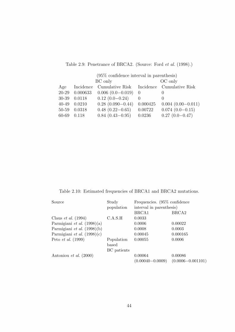
Table 2.9: Penetrance of BRCA2. (Source: Ford et al. (1998).)
(95% confidence interval in parenthesis)BC only OC only
Age Incidence Cumulative Risk Incidence Cumulative Risk20-29 0.000633 0.006 (0.0−0.019) 0 030-39 0.0118 0.12 (0.0−0.24) 0 040-49 0.0210 0.28 (0.090−0.44) 0.000425 0.004 (0.00−0.011)50-59 0.0318 0.48 (0.22−0.65) 0.00722 0.074 (0.0−0.15)60-69 0.118 0.84 (0.43−0.95) 0.0236 0.27 (0.0−0.47)
Table 2.10: Estimated frequencies of BRCA1 and BRCA2 mutations.
Source Study Frequencies. (95% confidencepopulation interval in parenthesis)
BRCA1 BRCA2Claus et al. (1994) C.A.S.H 0.0033Parmigiani et al. (1998)(a) 0.0006 0.00022Parmigiani et al. (1998)(b) 0.0008 0.0003Parmigiani et al. (1998)(c) 0.00045 0.000165Peto et al. (1999) Population 0.00055 0.0006
basedBC patients
Antoniou et al. (2000) 0.00064 0.00086(0.00040−0.0009) (0.0006−0.001101)
44

We note that frequencies given in Table 2.10 relate to the frequencies of the alleles
with a mutation. It should be taken into account that every woman has two alleles
each at BRCA1 and BRCA2 when calculating the distribution of the genotype. As
an example, the frequency estimates (a) by Parmigiani et al. (1998), given in Table
2.10, give the probability of a woman having one BRCA1 mutation and no BRCA2
mutation as 2× 0.0006× (1− 0.0006)× (1− 0.00022)2 = 0.001199.
For brevity we denote the frequency estimates (b) by Parmigiani et al. (1998),
that is a BRCA1 frequency of 0.0008 and BRCA2 frequency of 0.0003 as ‘high’
mutation frequencies. We also denote frequency estimates (c) by Parmigiani et al.
(1998), for which BRCA1 frequency is 0.00045 and BRCA2 frequency is 0.000165
as ‘low’ mutation frequencies. We will use this notation subsequently but note that
compared with the later BRCA2 frequency estimates (see Peto et al. (1999) and
Antoniou et al. (2000)) the BRCA2 frequency values used in our ‘high’ and ‘low’
frequency scenarios are lower.
BC or OC onset is assumed to be due to the presence of two mutations (the ‘two
hit hypothesis’). This can happen in one of three ways:
(a) A woman inherits mutations at both alleles of the BRCA1 or BRCA2 locus.
The gene function is lost in every cell of the woman’s body and is presumed to
be associated with an extremely high risk of cancer.
(b) A woman can inherit a mutation at a BRCA1 or BRCA2 allele and hence in all
cells in the body one allele at the locus is mutant and the other is normal (wild
type). The woman can then have a mutation at the wild type allele of the same
locus or at another gene locus. This new mutation is a somatic mutation and it
will be confined to the cell in which the mutation has taken place but the cells
that are derived from the mutant cell by cell division will have two mutations.
This scenario presents a high risk of cancer.
(c) A woman can be born with both alleles normal and then suffer a somatic muta-
tion at one allele in a cell. If that cell or any cells derived from it by cell division
further has a mutation at the wild type allele, then both alleles will be mutant.
The cells affected become potentially cancerous.
45

Cancer due to process (a) or (b) above is called hereditary cancer while that due
to process (c) is called sporadic cancer. Claus et al. (1996) estimate that about 7%
of BC and about 10% of OC cases in the general population are hereditary. Familial
cancer includes some sporadic cases.
2.4.2 BCOC genetics in clinical practice
In a clinical setting genetic testing for the presence of mutations is done if the
family history presented is associated with a very high probability that the woman
has a mutation. The results like those given by Claus et al. (1994) are meant to
help clinicians make this assessment of risk. Since the discovery of BRCA1 and
BRCA2, models to help in assessing carrier probabilities using the penetrance and
frequencies of these two genes have been devised. Parmigiani et al. (1998) give
one such model which is an improvement of the C.A.S.H. model since it includes
more relatives, unaffected relatives, BRCA1, BRCA2 and more information in its
modelling of the risk. The information normally required for the purpose of such
clinical risk estimation includes
(a) the number of blood relatives who have had BC and/or OC,
(b) their precise relationship to the woman whose risk is being assessed ( usually
called the proband),
(c) the ages at which they contracted cancer, and
(d) the clinical facts about their illness.
The amount of information actually used depends on the sophistication of the
model being used. This will also have an impact on the accuracy of the results. The
accuracy of the facts used is very important and medical records of relatives may
have to be checked to validate the given information. However a significant amount
of the information may have to be based on memory and thus compromise the results.
The output from using the models in risk assessment is usually the probability that
the woman carries BRCA1 or BRCA2 mutations. Based on that information, if it is
necessary, and following the required social and ethical procedures (like counselling),
a genetic test can be done. Aspects like counselling are very important parts of
genetic testing procedures and regulations. This is because the results will have
46

implications for other blood relatives as well as medical implications for the woman
tested, whether the test result is positive or not. A positive result will mean the
need for preventative measures and monitoring. A negative result does not mean
the woman cannot develop BC or OC. There is a need for careful analysis of the
results which takes into account the following factors.
(a) Little is known about the function of the proteins encoded by BRCA1 or
BRCA2.
(b) Most of the hundreds of known mutations have only been observed in one family.
This means that the risks of BC or OC in lives with the rare mutations may
be very different from the published estimates whose calculation was based on
lives with the common mutations.
(c) The genetic test used may not test for all known mutations or test the whole
gene. This is due to the high costs of the extensive tests.
(d) The test can not search for unknown mutations and there are, most likely,
mutations in BRCA1 or BRCA2 still unknown.
(e) There are other oncogenes affecting tumour formation, such as P53 and TPEN.
(f) There are almost certainly other breast and ovarian cancer genes as yet undis-
covered.
2.4.3 BCOC genetics applied to investigations into the im-
pact of BCOC on insurance
We note at this stage that other work that has been done to assess the impact of BC
and OC on insurance were based on family history models. Lemaire et al. (2000)
constructed the double decrement model shown in Figure 2.3 such that each age
and possible family history are represented by one such model. The probabilities of
developing BC (or OC) were derived from the risks of BC (or OC) for lives with a
particular family history as given in Claus et al. (1994).
Based on this model, in order to investigate the costs of adverse selection the
authors needed to make assumptions about the probability of a positive genetic test
result for a life with a specified family history (see Subramanian et al. (1999)). We
47
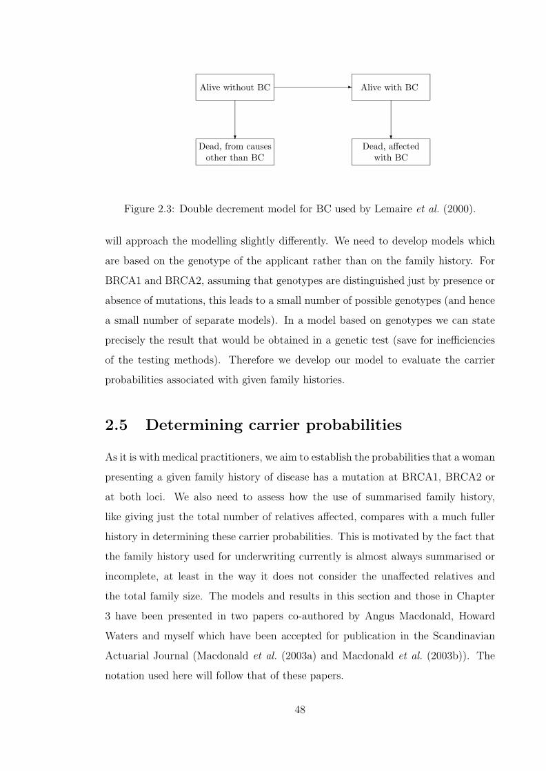
Dead, from causesother than BC
Dead, affectedwith BC
Alive without BC Alive with BC-
? ?
Figure 2.3: Double decrement model for BC used by Lemaire et al. (2000).
will approach the modelling slightly differently. We need to develop models which
are based on the genotype of the applicant rather than on the family history. For
BRCA1 and BRCA2, assuming that genotypes are distinguished just by presence or
absence of mutations, this leads to a small number of possible genotypes (and hence
a small number of separate models). In a model based on genotypes we can state
precisely the result that would be obtained in a genetic test (save for inefficiencies
of the testing methods). Therefore we develop our model to evaluate the carrier
probabilities associated with given family histories.
2.5 Determining carrier probabilities
As it is with medical practitioners, we aim to establish the probabilities that a woman
presenting a given family history of disease has a mutation at BRCA1, BRCA2 or
at both loci. We also need to assess how the use of summarised family history,
like giving just the total number of relatives affected, compares with a much fuller
history in determining these carrier probabilities. This is motivated by the fact that
the family history used for underwriting currently is almost always summarised or
incomplete, at least in the way it does not consider the unaffected relatives and
the total family size. The models and results in this section and those in Chapter
3 have been presented in two papers co-authored by Angus Macdonald, Howard
Waters and myself which have been accepted for publication in the Scandinavian
Actuarial Journal (Macdonald et al. (2003a) and Macdonald et al. (2003b)). The
notation used here will follow that of these papers.
48

We consider an applicant at age x. The family history they can present consists
of details of relatives affected with BC or OC prior to the time of application. For
each relative this means the life history of BC or OC from birth to their age when
the applicant applies for insurance. We are not primarily interested in the BC or
OC history of the applicant before they apply for insurance. The underwriting
requirements for CI policies are such that a life with a history of BC or OC is not
insurable. For the relatives we are only interested in the life history of BC and OC.
Any other previous illness does not contribute to family history in this regard.
2.5.1 Definitions
Family structure
Our starting point is the birth of the potential applicant for insurance. The smallest
possible family is the applicant and her mother. The applicant can also have sisters
and aunts. We define ‘family size’ as the number of female relatives including the
applicant, her mother, her sisters and her aunts, and denote it M . The family size
is at least 2. Both maternal and paternal aunts are included, but we omit cousins,
females of the grandparents’ generation and beyond, and all male relatives.
For simplicity, we assume that all the applicant’s sisters are the same age as she
is, and the mother and all aunts are 30 years older. A family structure specifies, in
addition to the applicant and her mother, which of the remaining M − 2 relatives
are sisters and which ones are aunts. The number of possible family structures, in
a family of size M , is then M − 1.
We label the family members i = 1, 2, . . . , M , and adopt the convention that the
applicant is always the first family member, and her mother the second. In a family
of size M , we denote the age of the ith member at the birth of the applicant xi
(x1 = 0 and x2 = 30 always and each xi for i > 2 is either 0 or 30), so the family
structure is represented by M and the vector:
X = (x1, x2, . . . , xM) (2.3)
or the pair (M,X). The omission of male relatives means that we ignore male breast
cancers.
49

Table 2.11: The population frequencies of the four genotypes (0, 0), (0, 1), (1, 0) and(1, 1), given the low and high estimates of mutation frequencies from Parmigianiet al. (1998).
.Allele Mutation Population Frequency of Genotype
Frequencies (0,0) (1,0) (0,1) (1,1)Low 0.998770525 0.000899501 0.000329675 0.000000299High 0.997801689 0.001598401 0.000598951 0.000000959
The genotypes of family members
Given a family structure, we assume known the BRCA1 and BRCA2 genotypes of
all its members. Each relative may have 0, 1 or 2 mutated copies of either gene.
There are nine possible genotypes, so in a family of size M there may be up to
9M combinations of genotypes. Genotypes like those in which the mother has no
mutation and the applicant has two mutations, are not feasible and will reduce
slightly the total number of combinations of genotypes. This reduction will have
little effect on any calculations and results.
We express the genotype by either the presence or absence of mutations, such that
having one mutated copy or having two mutated copies will not be distinguished.
Inheriting two BRCA1 or BRCA2 mutations is extremely rare (0.00082 for BRCA1
mutation using ‘high’ mutation frequencies). However should it happen, a mutation
will definitely be passed on to the offspring and as we noted before under the two hit
hypothesis, having two mutations is associated with very high disease risk. By not
distinguishing between heterozygous and homozygous mutation carriers we reduce
the possible genotype combinations to only 4M bringing the computations within
the reach of a fast computer. This approach is also necessitated by the fact that
BCOC penetrance of BRCA1 and BRCA2 (Tables 2.7 to 2.9) is given for mutation
carriers without distinguishing between homozygous and heterozygous carriers.
We denote the four genotypes (0, 0), (0, 1), (1, 0) and (1, 1) where ‘1’ in the first
place indicates a BRCA1 mutation, and in the second place a BRCA2 mutation. Ta-
ble 2.11 shows the frequencies of these genotypes given the ‘low’ and ‘high’ mutation
frequencies of Parmigiani et al. (1998) ((c) and (b) respectively in Table 2.10).
50
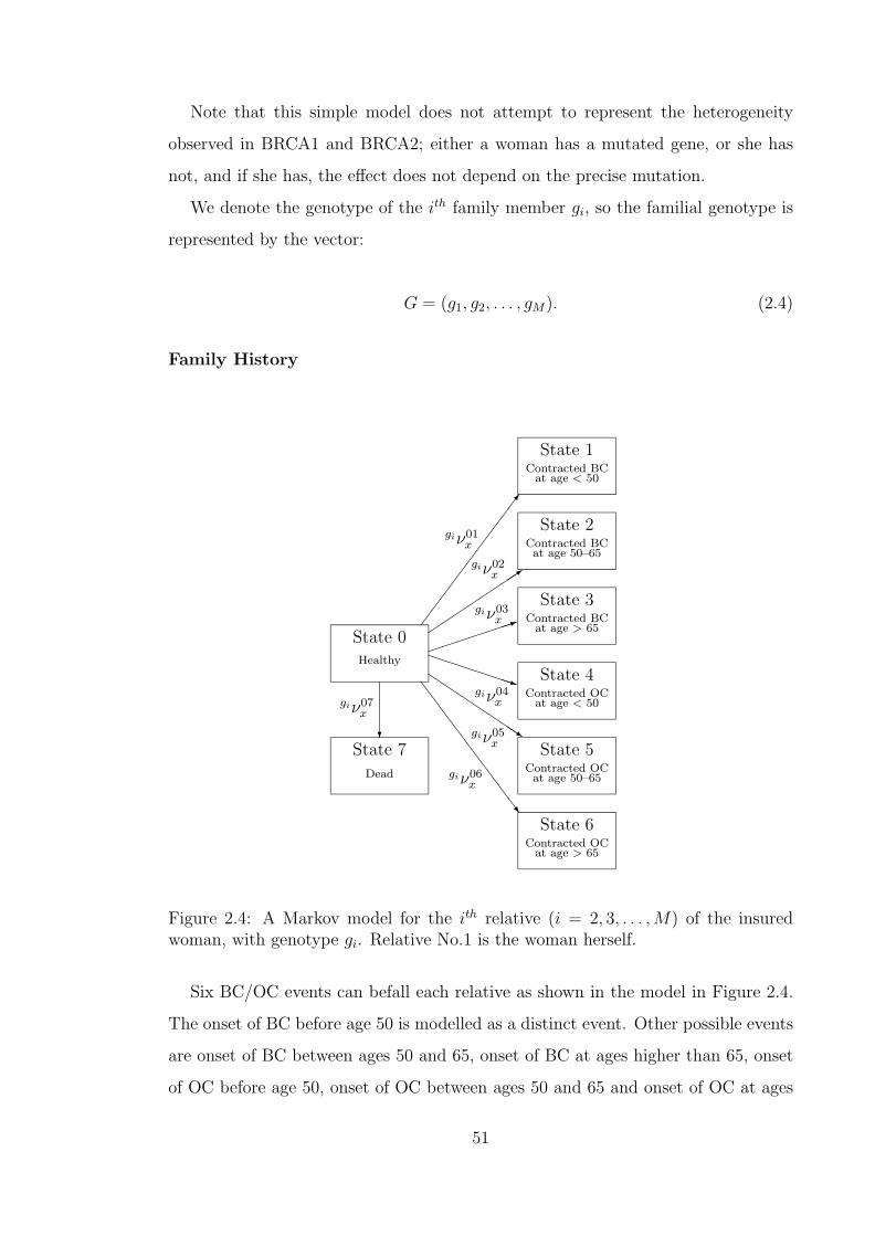
Note that this simple model does not attempt to represent the heterogeneity
observed in BRCA1 and BRCA2; either a woman has a mutated gene, or she has
not, and if she has, the effect does not depend on the precise mutation.
We denote the genotype of the ith family member gi, so the familial genotype is
represented by the vector:
G = (g1, g2, . . . , gM). (2.4)
Family History
SS
SS
SS
SS
Sw
QQQs
PPPPPPPq
³³³³³³³1´´
´´
´´3
¶¶
¶¶
¶¶
¶¶
¶7
?
State 0Healthy
State 1Contracted BC
at age < 50
State 2Contracted BCat age 50–65
State 3Contracted BC
at age > 65
State 4Contracted OC
at age < 50
State 5Contracted OCat age 50–65
State 6Contracted OC
at age > 65
State 7
Dead
giν01x
giν02x
giν03x
giν04x
giν05x
giν06x
giν07x
Figure 2.4: A Markov model for the ith relative (i = 2, 3, . . . , M) of the insuredwoman, with genotype gi. Relative No.1 is the woman herself.
Six BC/OC events can befall each relative as shown in the model in Figure 2.4.
The onset of BC before age 50 is modelled as a distinct event. Other possible events
are onset of BC between ages 50 and 65, onset of BC at ages higher than 65, onset
of OC before age 50, onset of OC between ages 50 and 65 and onset of OC at ages
51
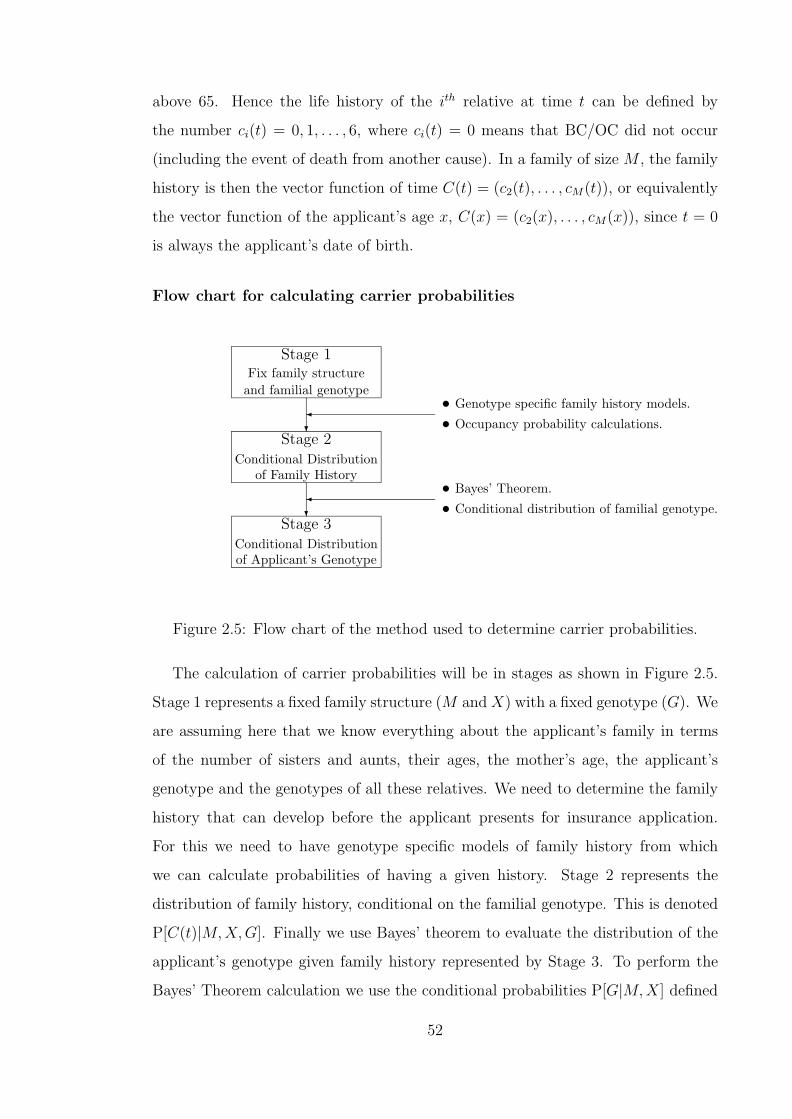
above 65. Hence the life history of the ith relative at time t can be defined by
the number ci(t) = 0, 1, . . . , 6, where ci(t) = 0 means that BC/OC did not occur
(including the event of death from another cause). In a family of size M , the family
history is then the vector function of time C(t) = (c2(t), . . . , cM(t)), or equivalently
the vector function of the applicant’s age x, C(x) = (c2(x), . . . , cM(x)), since t = 0
is always the applicant’s date of birth.
Flow chart for calculating carrier probabilities
?
?
Stage 1Fix family structureand familial genotype
Stage 2Conditional Distribution
of Family History
Stage 3Conditional Distributionof Applicant’s Genotype
¾ • Genotype specific family history models.
• Occupancy probability calculations.
¾ • Bayes’ Theorem.
• Conditional distribution of familial genotype.
Figure 2.5: Flow chart of the method used to determine carrier probabilities.
The calculation of carrier probabilities will be in stages as shown in Figure 2.5.
Stage 1 represents a fixed family structure (M and X) with a fixed genotype (G). We
are assuming here that we know everything about the applicant’s family in terms
of the number of sisters and aunts, their ages, the mother’s age, the applicant’s
genotype and the genotypes of all these relatives. We need to determine the family
history that can develop before the applicant presents for insurance application.
For this we need to have genotype specific models of family history from which
we can calculate probabilities of having a given history. Stage 2 represents the
distribution of family history, conditional on the familial genotype. This is denoted
P[C(t)|M,X,G]. Finally we use Bayes’ theorem to evaluate the distribution of the
applicant’s genotype given family history represented by Stage 3. To perform the
Bayes’ Theorem calculation we use the conditional probabilities P[G|M,X] defined
52
as the probability that the familial genotype is G, given the family size M and the
ages X, i.e. given family structure (M,X), as will be shown later in Section 2.5.3.
Determining the family history given the familial genotype involves the develop-
ment and parameterisation of a genotype specific family history model. To improve
the flow of the discussion, this development and parameterisation will be discussed
first (in Section 2.5.2) before using the results with the rest of the flow chart to
determine carrier probabilities.
As it stands the approach detailed in the last two paragraphs should achieve the
first aim set out in Section 2.5; that of estimating carrier probabilities given family
history. However the second aim is to assess the value of summarised, incomplete
family history. We will extend the process shown in the flow chart as follows: instead
of fixing the family structure, we use the distribution of family structures. Using
this distribution of family structure, we can calculate carrier probabilities given
family history, using various summaries of family history. This extension requires
the estimation of the distribution of family structures, P[M,X]. This will be done
in Section 2.5.5.
2.5.2 Model for relative’s BCOC history
Model representation
In Figure 2.4 we presented an eight-state Markov model to represent the life of any
of the applicant’s relatives. As shown, a life starts in State 0, the healthy state. The
model represents movements due to BC, OC or death only and therefore a relative
remains in the healthy state until the first of these three events happens. It means
that the ‘Healthy’ state will include lives who have had illnesses like cancers other
than BC or OC, heart attacks or strokes.
From the healthy state a life can develop BC. In our modelling, as is the case
in the clinical setting, the age at onset of any affected relative is of interest. For
the model to capture the age at onset and also the age of the relative at the time
of presentation by the applicant, it has to capture the duration of the disease since
onset. This can be handled by a semi-Markov model, but with considerable difficulty
in terms of tractability. For the model to be Markov, a life which develops BC moves
53

into a state which incorporates the information about age at onset. The BC states,
States 1 to 3, reflect the broad groups into which ages at onset have been assigned
by underwriters, as shown in Tables 2.3 and 2.4. A life can also develop OC and
the state they move to similarly depends on the age at onset. Once a relative
develops BC or OC then we are not interested in their future life history. A life
which dies before developing BC or OC moves to the ‘Dead’ state. At the point
of death their complete life history is fixed as ‘unaffected’ relatives at the age of
death. This is in contrast to lives who die after contracting BC or OC, whose death
adds nothing to their life history. This is so because events after onset of BC or
OC will not give information about the probability of getting BC or OC. However,
although information about events after onset is currently neither collected nor
used for underwriting, it may be relevant in models of life insurance rather than CI
insurance.
We assume that there are M relatives (including the applicant) and the ith rel-
ative has genotype gi. We use the convention that the first relative (i = 1) is the
applicant herself. Each of the M−1 relatives of the applicant have their life histories
represented by a model such as Figure 2.4. We denote the 8 states of the model by
j = 0, 1, 2, . . . , 7 and the transition intensities between state 0 and state j (j 6= 0)
by giν0jx . The notation giν0j
x reflects the fact that the transition intensities depend
on the genotype of the individual. Should this not have been so, then we would not
reflect the heterogeneity in BC and OC risk due to genotype.
If we further define giνx =∑j=7
j=1giν0j
x , then the probability that the ith relative
is in state j at age x + t, given that she was healthy at age x, will be denoted gip0jx,t
and we have:
gip00x,t = exp
−
t∫0
giνx+sds
, (2.5)
gip0jx,t =
t∫0
gip00x,s
giν0jx+sds (j = 1, . . . , 7). (2.6)
54

Equations (2.5) and (2.6) are occupancy probabilities within a multiple state
model as described in Waters (1984) and Macdonald (1996a). The fact that all
states apart from state 0 in Figure 2.4 are absorbing states make these equations
straight forward to write out.
Estimating the transition intensities of the model
To complete the specification of the model in Figure 2.4 we need to specify the
transition intensities in the model. These intensities fall into three groups.
(a) The intensities of BC and OC in lives without any mutation at BRCA1 or
BRCA2. These are assumed to be adequately represented by the intensities of
BC and OC in the general population.
(b) The intensities of BC and OC in lives with mutations at either BRCA1, BRCA2
or both.
(c) The mortality of lives who have not had either BC or OC.
BC and OC incidence in non-mutation carriers
We assume a period of investigation of three years from 1 January 1990 to 31 De-
cember 1992. The CD ROM O.N.S. (1999) contains details of registrations by year,
age at registration, site of cancer, sex of patient among other characteristics for
all cancers diagnosed in the U.K from 1971 to 1992. We extracted details on the
breast cancer cases registered during our period of investigation. These were used
to determine the number of new BC cases by single year of age in the whole three
year period. We note that the publications O.N.S (1997b, 1998a, 1998b) give the
same data but grouped into five-year age bands. We grouped our results based on
O.N.S. (1999) and compared the data with that from O.N.S (1997b, 1998a, 1998b).
The two sets agreed satisfactorily.
We denote the number of new cases of BC in lives aged x, θx. The age is defined
as just age at diagnosis and we assume it refers to the age at the last birthday before
diagnosis. The exposed to risk (time for which lives are exposed to risk of BC) for
between ages x and x + 1 in the investigation period, Ecx is
55
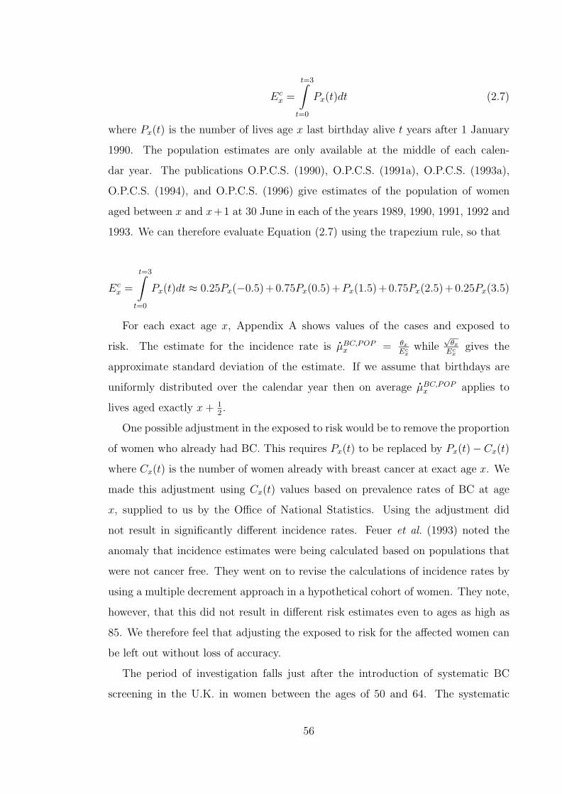
Ecx =
t=3∫t=0
Px(t)dt (2.7)
where Px(t) is the number of lives age x last birthday alive t years after 1 January
1990. The population estimates are only available at the middle of each calen-
dar year. The publications O.P.C.S. (1990), O.P.C.S. (1991a), O.P.C.S. (1993a),
O.P.C.S. (1994), and O.P.C.S. (1996) give estimates of the population of women
aged between x and x+1 at 30 June in each of the years 1989, 1990, 1991, 1992 and
1993. We can therefore evaluate Equation (2.7) using the trapezium rule, so that
Ecx =
t=3∫t=0
Px(t)dt ≈ 0.25Px(−0.5)+0.75Px(0.5)+Px(1.5)+0.75Px(2.5)+0.25Px(3.5)
For each exact age x, Appendix A shows values of the cases and exposed to
risk. The estimate for the incidence rate is µBC,POPx = θx
Ecx
while√
θx
Ecx
gives the
approximate standard deviation of the estimate. If we assume that birthdays are
uniformly distributed over the calendar year then on average µBC,POPx applies to
lives aged exactly x + 12.
One possible adjustment in the exposed to risk would be to remove the proportion
of women who already had BC. This requires Px(t) to be replaced by Px(t)−Cx(t)
where Cx(t) is the number of women already with breast cancer at exact age x. We
made this adjustment using Cx(t) values based on prevalence rates of BC at age
x, supplied to us by the Office of National Statistics. Using the adjustment did
not result in significantly different incidence rates. Feuer et al. (1993) noted the
anomaly that incidence estimates were being calculated based on populations that
were not cancer free. They went on to revise the calculations of incidence rates by
using a multiple decrement approach in a hypothetical cohort of women. They note,
however, that this did not result in different risk estimates even to ages as high as
85. We therefore feel that adjusting the exposed to risk for the affected women can
be left out without loss of accuracy.
The period of investigation falls just after the introduction of systematic BC
screening in the U.K. in women between the ages of 50 and 64. The systematic
56

screening programme was started in 1988 and all women in this age group are invited
for screening every three years. This resulted in a steep increase in incidence rates
for the screened ages compared to the other ages. This was noted by Quinn and
Allen (1995) in their paper which considered the influence of systematic screening
on the incidence of BC in England and Wales. There is a lag in the publication
of cancer incidence statistics and it may be a few years before the true level of the
incidence is established. Quinn and Allen (1995) state that the recorded incidence
from 1994 onwards is expected to return to the pre-screening levels except for the
50–52 age group. This age group is expected to continue with the high recorded
incidence rates because the first screening cycle for a cohort is expected to be in this
age group.
We considered the shape of the incidence curve before the systematic screen-
ing was started using data from O.N.S. (1999) for the years 1984 to 1988. This
assessment, together with the conclusion from Quinn and Allen (1995), led to the
conclusion that any function to represent the long term incidence of BC (as triggered
by diagnosis) should not follow the high rates for ages 53 to 64 found in the rates
from 1990 to 1992. However the function should reflect the elevated rates at ages
50 to 52.
The incidence of BC was modelled, by unweighted least squares, using two func-
tions as follows
µBC,POPx =
1Γ(8.7305)
0.07428.7305e−0.0742xx7.7305 for 0 ≤ x < 53
0.00012 + 0.00018(x− 35)− 0.000005(x− 35)2
+0.0000000529(x− 35)3 for x ≥ 53.
(2.8)
The observed rates and the fitted functions are shown in Figure 2.6. The function
for ages 53 and above was fitted using only data from ages 65 and above. We note
that the expression for ages below 53 can also be expressed as 6.0424 × 10⁻¹⁵ ×e−0.0742xx7.7305. We will apply the form used in Equation 2.8 in subsequent expres-
sions.
57
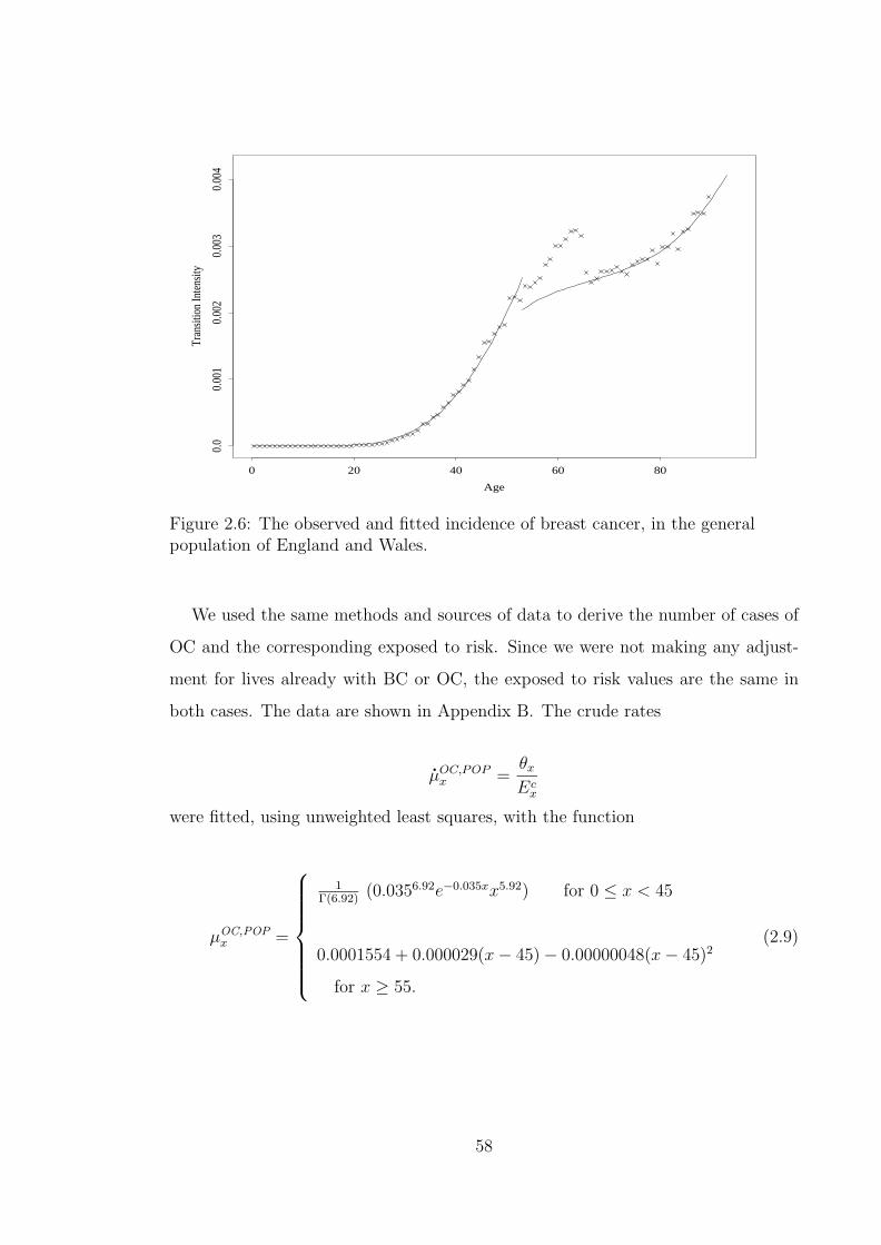
Age
Tran
sitio
n In
tens
ity
0 20 40 60 80
0.0
0.00
10.
002
0.00
30.
004
Figure 2.6: The observed and fitted incidence of breast cancer, in the generalpopulation of England and Wales.
We used the same methods and sources of data to derive the number of cases of
OC and the corresponding exposed to risk. Since we were not making any adjust-
ment for lives already with BC or OC, the exposed to risk values are the same in
both cases. The data are shown in Appendix B. The crude rates
µOC,POPx =
θx
Ecx
were fitted, using unweighted least squares, with the function
µOC,POPx =
1Γ(6.92)
(0.0356.92e−0.035xx5.92) for 0 ≤ x < 45
0.0001554 + 0.000029(x− 45)− 0.00000048(x− 45)2
for x ≥ 55.
(2.9)
58
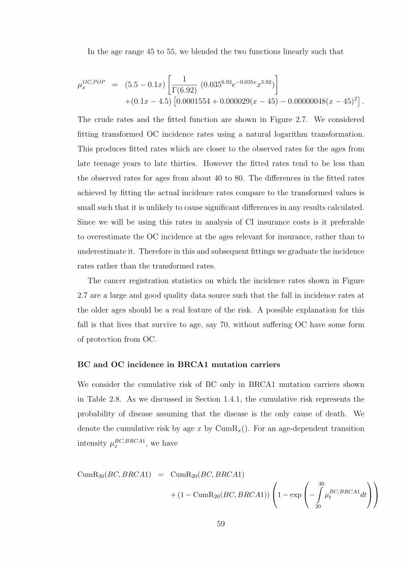
In the age range 45 to 55, we blended the two functions linearly such that
µOC,POPx = (5.5− 0.1x)
[1
Γ(6.92)(0.0356.92e−0.035xx5.92)
]+(0.1x− 4.5)
[0.0001554 + 0.000029(x− 45)− 0.00000048(x− 45)2
].
The crude rates and the fitted function are shown in Figure 2.7. We considered
fitting transformed OC incidence rates using a natural logarithm transformation.
This produces fitted rates which are closer to the observed rates for the ages from
late teenage years to late thirties. However the fitted rates tend to be less than
the observed rates for ages from about 40 to 80. The differences in the fitted rates
achieved by fitting the actual incidence rates compare to the transformed values is
small such that it is unlikely to cause significant differences in any results calculated.
Since we will be using this rates in analysis of CI insurance costs is it preferable
to overestimate the OC incidence at the ages relevant for insurance, rather than to
underestimate it. Therefore in this and subsequent fittings we graduate the incidence
rates rather than the transformed rates.
The cancer registration statistics on which the incidence rates shown in Figure
2.7 are a large and good quality data source such that the fall in incidence rates at
the older ages should be a real feature of the risk. A possible explanation for this
fall is that lives that survive to age, say 70, without suffering OC have some form
of protection from OC.
BC and OC incidence in BRCA1 mutation carriers
We consider the cumulative risk of BC only in BRCA1 mutation carriers shown
in Table 2.8. As we discussed in Section 1.4.1, the cumulative risk represents the
probability of disease assuming that the disease is the only cause of death. We
denote the cumulative risk by age x by CumRx(). For an age-dependent transition
intensity µBC,BRCA1x , we have
CumR30(BC, BRCA1) = CumR20(BC, BRCA1)
+ (1− CumR20(BC, BRCA1))
1− exp
−
30∫20
µBC,BRCA1t dt
59
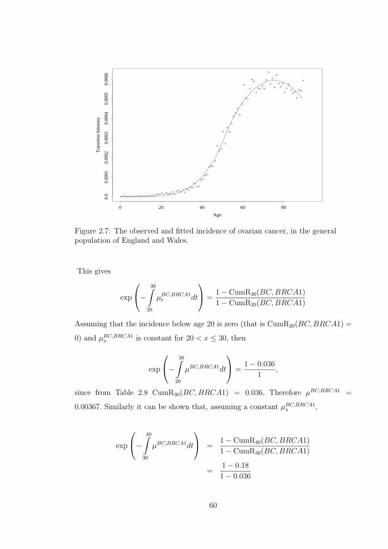
Age
Tran
sitio
n In
tens
ity
0 20 40 60 80
0.0
0.00
010.
0002
0.00
030.
0004
0.00
050.
0006
Figure 2.7: The observed and fitted incidence of ovarian cancer, in the generalpopulation of England and Wales.
This gives
exp
−
30∫20
µBC,BRCA1t dt
=
1− CumR30(BC,BRCA1)
1− CumR20(BC,BRCA1)
Assuming that the incidence below age 20 is zero (that is CumR20(BC,BRCA1) =
0) and µBC,BRCA1x is constant for 20 < x ≤ 30, then
exp
−
30∫20
µBC,BRCA1dt
=
1− 0.036
1,
since from Table 2.8 CumR30(BC,BRCA1) = 0.036. Therefore µBC,BRCA1 =
0.00367. Similarly it can be shown that, assuming a constant µBC,BRCA1x ,
exp
−
40∫30
µBC,BRCA1dt
=
1− CumR40(BC,BRCA1)
1− CumR30(BC,BRCA1)
=1− 0.18
1− 0.036
60

again using values from Table 2.8. This gives us µBC,BRCA1 = 0.01618. We repeat
the above with the rest of the age groups in the table to get the incidence rates
shown in Table 2.12.
Table 2.12: Incidence of BC and OC in BRCA1 mutation carriers.
Age Group20–29 30–39 40–49 50–59 60–69
Breast Cancer 0.00367 0.01618 0.04749 0.03483 0.02162Ovarian Cancer 0 0 0.01706 0.01947 0.01692
We fitted the truncated Gamma function
µBC,BRCA1x =
1.25
Γ(22)(0.4522e−0.45xx21) (2.10)
to the intensities. It was preferable to graduate the intensities , as opposed to the
cumulative risk, because our model is defined in terms of intensities. The fitted
function, extrapolated to age 90, and the crude rates are shown in Figure 2.8. In
choosing the truncated Gamma function we follow Parmigiani et al. (1998), although
they fitted the gamma cumulative distribution function to the cumulative rates.
To assess the fitted intensities we use Equation (2.10) to model the cumulative
risk of BC in BRCA1 mutation carriers which we compare with the values in Table
2.8. These results are shown in Table 2.13 and show that the modelled risk is within
the 95% confidence intervals given by Ford et al. (1998) (Table 2.8). The modelled
cumulative risk is calculated as
Cumulative risk at age x = 1− exp
−
x∫0
1.25
Γ(22)(0.4522e−0.45ss21)ds
.
Surviving to age x free of BC or OC means surviving free of BC and independently
surviving free of OC. This assumption of additive BC and OC intensities in mutation
carriers is reasonable since the mutations are affecting different organs of the body.
Therefore
1−CumRx(BC or OC) = (1−CumRx(BC only))×(1−CumRx(OC only)). (2.11)
61
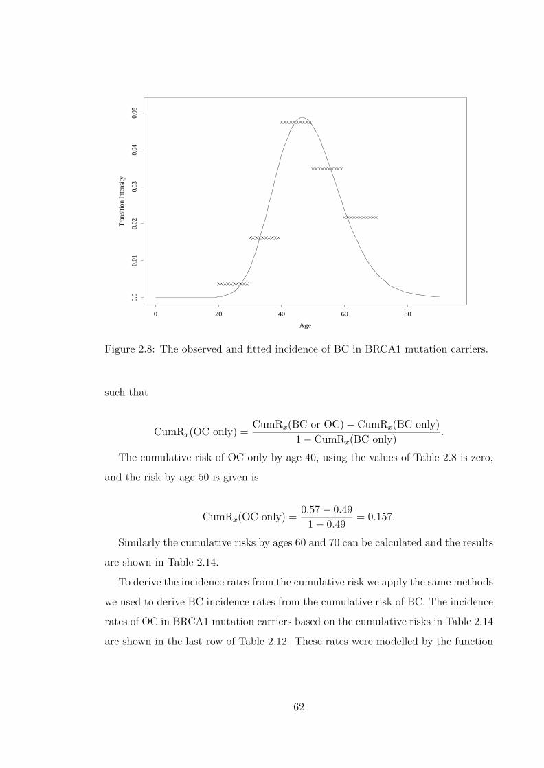
Age
Tran
sitio
n In
tens
ity
0 20 40 60 80
0.0
0.01
0.02
0.03
0.04
0.05
Figure 2.8: The observed and fitted incidence of BC in BRCA1 mutation carriers.
such that
CumRx(OC only) =CumRx(BC or OC)− CumRx(BC only)
1− CumRx(BC only).
The cumulative risk of OC only by age 40, using the values of Table 2.8 is zero,
and the risk by age 50 is given is
CumRx(OC only) =0.57− 0.49
1− 0.49= 0.157.
Similarly the cumulative risks by ages 60 and 70 can be calculated and the results
are shown in Table 2.14.
To derive the incidence rates from the cumulative risk we apply the same methods
we used to derive BC incidence rates from the cumulative risk of BC. The incidence
rates of OC in BRCA1 mutation carriers based on the cumulative risks in Table 2.14
are shown in the last row of Table 2.12. These rates were modelled by the function
62

Table 2.13: Modelled cumulative risks of breast cancer, and breast or ovarian cancerin BRCA1 mutation carriers compared with observed rates and 95% confidenceintervals in Table 2.8.
Breast Cancer Breast Cancer or Ovarian CancerObserved Modelled Observed Modelled
Cumulative Confidence Cumulative Cumulative Confidence CumulativeAge x Risk Interval Risk Risk Interval Risk
30 0.036 0–0.14 0.0252 0.036 0–0.14 0.028240 0.18 0–0.35 0.2221 0.18 0–0.36 0.256250 0.49 0.28–0.64 0.5097 0.57 0.33–0.73 0.593060 0.64 0.43–0.77 0.6572 0.75 0.53–0.87 0.765070 0.71 0.53–0.82 0.7020 0.83 0.65–0.92 0.8218
Table 2.14: Cumulative risk of OC only in BRCA1 mutation carriers
Age 30 40 50 60 70Cumulative Risk 0 0 0.1568 0.306 0.414
µOC,BRCA1x =
0.60
Γ(21)(0.3721e−0.37xx20). (2.12)
and Figure 2.9 shows the function together with the incidence rates.
By rearranging Equation (2.11), and substituting the fitted functions µBC,BRCA1x
and µOC,BRCA1x the cumulative risk of BC or OC in BRCA1 mutation carriers can
be modelled by
CumRx(BC or OC) = 1− exp
−
x∫0
(µBC,BRCA1
s + µOC,BRCA1s
)ds
.
In Table 2.13 we show that these modelled rates all fall within the 95% confidence
intervals for the rates given by Ford et al. (1998) which we presented in Table 2.8.
BC and OC incidence in BRCA2 mutation carriers
We showed in Table 2.9 the incidence of BC and OC in BRCA2 mutation carriers
given by Ford et al. (1998). Confidence intervals for risk estimates were only given
63

Age
Tran
sitio
n In
tens
ity
0 20 40 60 80
0.0
0.00
50.
010
0.01
50.
020
Figure 2.9: The observed and fitted incidence of OC in BRCA1 mutation carriers.
for the cumulative risk and not for the incidence. The incidence rates were modelled
with the functions
µBC,BRCA2x =
3.60
Γ(30)(0.4530e−0.45xx29) (2.13)
for BC and
µOC,BRCA2x =
0.86
Γ(27)(0.35527e−0.355xx26) (2.14)
for OC. The incidence rates and the fitted functions are shown in Figures 2.10 and
2.11.
The fitted function models well the cumulative risk such that the modelled risk
falls within the 95% confidence intervals of the estimated risk. This comparison
for BRCA2 mutation carriers is shown in Table 2.15. The adequacy of the fitted
functions is shown in Figure 2.12 which plots the modelled cumulative risks of BC
and OC in mutation carriers alongside the observed rates.
64

Age
Tran
sitio
n In
tens
ity
0 20 40 60 80
0.0
0.02
0.04
0.06
0.08
0.10
0.12
Figure 2.10: The observed and fitted incidence of BC in BRCA2 mutation carriers.
Up to this stage we have not specified the exact definition of “mutation” carriers
with respect to BRCA1 and BRCA2, with which the risk estimates used so far
are associated. Using ‘high’ mutation frequencies, the probability that a woman
inherits two BRCA1 mutations is 6.4× 10⁻⁷ ( i.e. 0.00082) and the probability that
she inherits two BRCA2 mutations is 9.0 × 10⁻⁸ ( i.e. 0.00032). These are so rare
that is only logical to assume that lives on which the risk estimates are based inherit
only one mutation. Consequently the functions fitted for the incidence of BC or OC
in mutation carriers (formulae (2.10), (2.12), (2.13), and (2.14)) apply to lives who
inherit one mutation at the appropriate locus. We also assume that should a woman
inherit two mutations at one locus, then the risk of either BC or OC are the same
as that of a woman who inherits one mutation.
A woman can inherit mutations at both BRCA1 and BRCA2. The probability
of this happening is of the same order of magnitude as the probability of having two
mutations at one of the two loci. Cancer due to BRCA1 and cancer due to BRCA2
are independent events, as noted by Parmigiani et al. (1998), and we have assumed
65

Age
Tran
sitio
n In
tens
ity
0 20 40 60 80
0.0
0.00
50.
010
0.01
50.
020
Figure 2.11: The observed and fitted incidence of OC in BRCA2 mutation carriers.
that the incidence rates for women with mutations at both loci are equal to the
sum of the individual incidence rates. This is different to the approach by Antoniou
et al. (2000) whereby they assume that BRCA1 dominates BRCA2, meaning that
for women with mutations at both loci, the incidence rates applicable to BRCA1
are used. Using either approach is likely to lead to similar results due to the rarity
of having mutations at both loci.
Figures 2.13 and 2.14 summarise all the intensities of BC or OC by all the possible
genotypes for use in our relatives model.
Mortality rates in respect of lives without BC and OC
The mortality transition in the model in Figure 2.4 is for lives who have not devel-
oped BC or OC. The life table ELT15F is based on all lives in England and Wales
(with or without BC or OC) between 1990 and 1992. We note that the crude force
of mortality is
µELT15Fx =
θELT15Fx
EELT15Fx
66
Table 2.15: Modelled cumulative risks of breast cancer and ovarian cancer in BRCA2mutation carriers compared with observed rates and 95% confidence intervals inTable 2.9.
Breast Cancer Ovarian CancerObserved Modelled Observed Modelled
Cumulative Confidence Cumulative Cumulative Confidence CumulativeAge x Risk Interval Risk Risk Interval Risk
30 0.006 0–0.019 0.0003 0 n/a < 0.000140 0.12 0–0.240 0.0212 0 n/a 0.001450 0.28 0.09–0.440 0.2359 0.004 0.00–0.011 0.020760 0.48 0.22–0.650 0.6683 0.074 0.00–0.150 0.106870 0.84 0.43–0.950 0.8962 0.27 0.00–0.470 0.2657
where θELT15Fx and EELT15F
x are the deaths and exposed to risk used for the ELT15F
estimation. We split both the deaths and exposure into two parts; one corresponding
to the population which is free of disease (θNx and EN
x ) and another corresponding
to the population with BC or OC (θDx and ED
x ). θELT15Fx = θN
x + θDx and
EELT15Fx = EN
x + EDx . We note that
µELT15Fx =
θELT15Fx
EELT15Fx
=θN
x + θDx
ENx + ED
x
=θN
x
ENx + ED
x
+θD
x
ENx + ED
x
× θELT15Fx
θELT15Fx
=θN
x
ENx + ED
x
+θD
x
θELT15Fx
× µELT15Fx ,
which gives
θNx
ENx + ED
x
= µELT15Fx
(1− θD
x
θELT15Fx
). (2.15)
The left hand side of Equation (2.15) is approximately equal to the required µNx = θN
x
ENx
if EDx is much smaller that EN
x . Based on data supplied to us by the O.N.S, the
age specific prevalence of BC in the population peaked at about 0.016 around ages
64 to 80. We feel it is reasonable to assume that the exposed to risk for mortality
estimation will be much smaller in BC patients than in the rest of the population.
Replacing µELT15Fx in Equation (2.15) with the graduated force of mortality µELT15F
x ,
we will represent the mortality of disease free lives by the expression
67
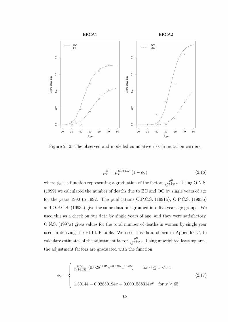
BRCA1
Age
Cum
ulat
ive
risk
20 30 40 50 60 70 80
0.0
0.2
0.4
0.6
0.8
BCOC
BRCA2
Age
Cum
ulat
ive
risk
20 30 40 50 60 70 800.
00.
20.
40.
60.
8
BCOC
Figure 2.12: The observed and modelled cumulative risk in mutation carriers.
µNx = µELT15F
x (1− φx) (2.16)
where φx is a function representing a graduation of the factors θDx
θELT15Fx
. Using O.N.S.
(1999) we calculated the number of deaths due to BC and OC by single years of age
for the years 1990 to 1992. The publications O.P.C.S. (1991b), O.P.C.S. (1993b)
and O.P.C.S. (1993c) give the same data but grouped into five year age groups. We
used this as a check on our data by single years of age, and they were satisfactory.
O.N.S. (1997a) gives values for the total number of deaths in women by single year
used in deriving the ELT15F table. We used this data, shown in Appendix C, to
calculate estimates of the adjustment factor θDx
θELT15Fx
. Using unweighted least squares,
the adjustment factors are graduated with the function
φx =
8.63Γ(14.05)
(0.02814.05e−0.028xx13.05) for 0 ≤ x < 54
1.30144− 0.02850194x + 0.0001588314x2 for x ≥ 65,
(2.17)
68
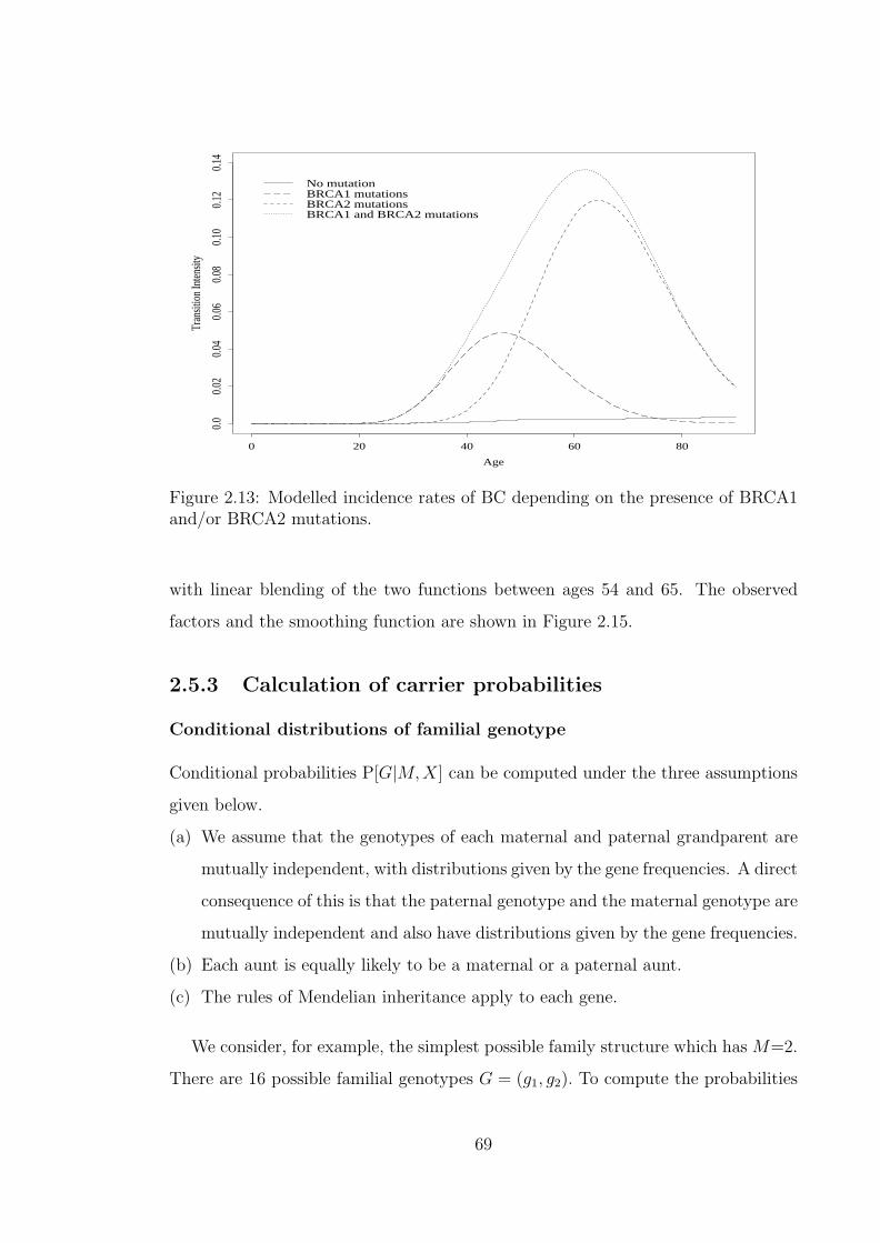
Age
Tran
sitio
n In
tensit
y
0 20 40 60 80
0.0
0.02
0.04
0.06
0.08
0.10
0.12
0.14
No mutationBRCA1 mutationsBRCA2 mutationsBRCA1 and BRCA2 mutations
Figure 2.13: Modelled incidence rates of BC depending on the presence of BRCA1and/or BRCA2 mutations.
with linear blending of the two functions between ages 54 and 65. The observed
factors and the smoothing function are shown in Figure 2.15.
2.5.3 Calculation of carrier probabilities
Conditional distributions of familial genotype
Conditional probabilities P[G|M,X] can be computed under the three assumptions
given below.
(a) We assume that the genotypes of each maternal and paternal grandparent are
mutually independent, with distributions given by the gene frequencies. A direct
consequence of this is that the paternal genotype and the maternal genotype are
mutually independent and also have distributions given by the gene frequencies.
(b) Each aunt is equally likely to be a maternal or a paternal aunt.
(c) The rules of Mendelian inheritance apply to each gene.
We consider, for example, the simplest possible family structure which has M=2.
There are 16 possible familial genotypes G = (g1, g2). To compute the probabilities
69

Age
Tran
sitio
n In
tensit
y
0 20 40 60 80
0.0
0.01
0.02
0.03
No mutationBRCA1 mutationsBRCA2 mutationsBRCA1 and BRCA2 mutations
Figure 2.14: Modelled incidence rates of OC depending on the presence of BRCA1and/or BRCA2 mutations.
associated with each of the 16 familial genotypes, we could proceed by fixing the
mother’s genotype and calculating the conditional distribution of the daughter’s
genotype. Thus P[g1, g2] = P[g1|g2]P[g2]. Examples of probabilities P[g2] are shown
in Table 2.11 and these involve gene frequencies in their calculation. P[g1|g2] is
calculated by summing over the probabilities of all compatible genotypes of the
father (whose distribution is also determined by gene frequencies). The distribution
of familial genotypes for the family of size 2 is shown in the Table 2.16.
In practice with family sizes higher than 2, a computer program is required to gen-
erate all the possibilities and calculate the probabilities from first principles. The
calculations are computationally intensive and this determined the largest family
size with which we could work (M = 10). Computing complete tables of P[G|M,X]
for M ≤ 10, and for ‘high’ and ‘low’ estimates of mutation frequencies, took almost
a month of CPU time on the fastest computer available to us. The difficulty is en-
hanced by the fact that we do not distinguish between maternal and paternal aunts
in the family structure X, but must do so here by considering all possible combina-
tions, given the total number of aunts. However, the simpler family structure makes
70
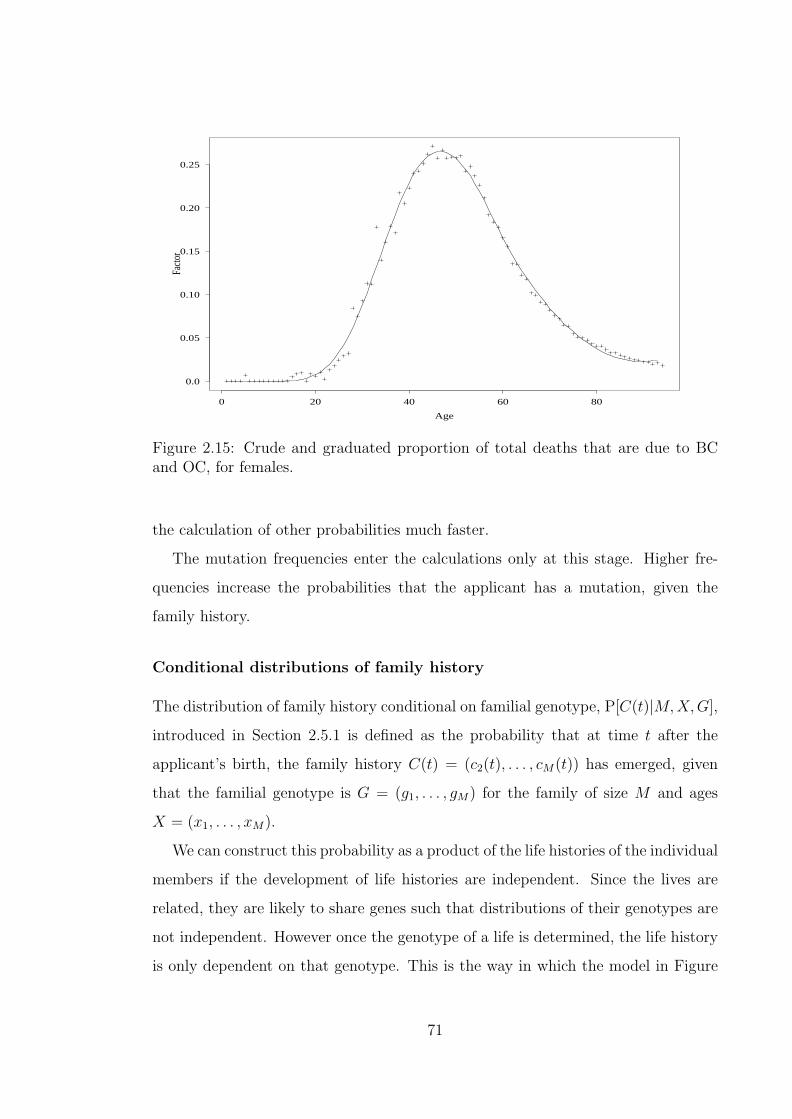
Age
Facto
r
0 20 40 60 80
0.0
0.05
0.10
0.15
0.20
0.25
Figure 2.15: Crude and graduated proportion of total deaths that are due to BCand OC, for females.
the calculation of other probabilities much faster.
The mutation frequencies enter the calculations only at this stage. Higher fre-
quencies increase the probabilities that the applicant has a mutation, given the
family history.
Conditional distributions of family history
The distribution of family history conditional on familial genotype, P[C(t)|M,X,G],
introduced in Section 2.5.1 is defined as the probability that at time t after the
applicant’s birth, the family history C(t) = (c2(t), . . . , cM(t)) has emerged, given
that the familial genotype is G = (g1, . . . , gM) for the family of size M and ages
X = (x1, . . . , xM).
We can construct this probability as a product of the life histories of the individual
members if the development of life histories are independent. Since the lives are
related, they are likely to share genes such that distributions of their genotypes are
not independent. However once the genotype of a life is determined, the life history
is only dependent on that genotype. This is the way in which the model in Figure
71

Table 2.16: Distribution of familial genotypes for families of size 2. ‘Low’ estimatesof mutation frequencies.
Familial Genotype Probability Familial Genotype Probability(0,0),(0,0) 0.99815635700 (0,0),(0,1) 0.00016472000(0,1),(0,0) 0.00016472300 (0,1),(0,1) 0.00016480000(1,0),(0,0) 0.00044937300 (1,0),(0,1) 0.00000007416(1,1),(0,0) 0.00000007416 (1,1),(0,1) 0.00000007420(0,0),(1,0) 0.00044937300 (0,0),(1,1) 0.00000007416(0,1),(1,0) 0.00000007416 (0,1),(1,1) 0.00000007420(1,0),(1,0) 0.00044998000 (1,0),(1,1) 0.00000007426(1,1),(1,0) 0.00000007426 (1,1),(1,1) 0.00000007430
2.4 has been formulated. Formally if we define random variables Ti for i = 1, . . . ,M
such that Ti represents the future lifetimes, free of BC and OC, of relative i, then the
Ti’s are unlikely to be mutually unconditionally independent. Since we assume that
G is known, it means the genotype of each relative is given by G. The life histories
of the relatives, conditioned on the common G can be taken as independent.
It is also assumed that at the time the applicant is born, the mother is free of
BC or OC. The calculation of P[C(t)|M,X,G] will split into two cases; one in which
the life history of the mother has BC or OC and the other in which her history is
free of BC or OC (but including the possibility of death before BC or OC).
Using Equations (2.5) and (2.6), we note the following expressions.
(a) g2p000,30+t = g2p00
0,30 × g2p0030,t and g2p07
0,30+t = g2p070,30 + g2p00
0,30 × g2p0730,t
so that the probability that the mother is free of BC or OC, or is dead without
BC or OC, at time t years after age 30 (i.e c2(t) = 0) is given by
g2p0030,t + g2p07
30,t =g2p00
0,30+t + g2p070,30+t − g2p07
0,30
g2p000,30
.
(b) g2p0c2(t)0,30+t = g2p
0c2(t)0,30 + g2p00
0,30 × g2p0c2(t)30,t
so that the probability that the mother has had BC or OC by time t years after
the birth of the applicant (i.e c2(t) > 0) is
g2p0c2(t)30,t =
g2p0c2(t)0,30+t − g2p
0c2(t)0,30
g2p000,30
.
(c) For any other relative who is not the mother, including the applicant, the prob-
ability of not having BC or OC before time t after the applicant’s birth is
72

gip000,xi+t + gip07
0,xi+t. The probability that the relative has BC or OC before the
applicant is aged t years is gip0ci(t)0,xi+t.
The probability P[C(t)|M,X,G] is therefore expressed in two parts as
P[C(t)|M, X, G] =g2p00
0,30+t + g2p070,30+t − g2p07
0,30
g2p000,30
∏i6=2
ci(t)=0
(gip000,xi+t + gip07
0,xi+t)∏i6=2
ci(t)>0
gip0ci(t)0,xi+t
(2.18)
if c2(t) = 0, and:
P[C(t)|M, X, G] =g2p
0c2(t)0,30+t − g2p
0c2(t)0,30
g2p000,30
∏i6=2
ci(t)=0
(gip000,xi+t + gip07
0,xi+t)∏i6=2
ci(t)>0
gip0ci(t)0,xi+t (2.19)
if c2(t) > 0. In each case, the first product is over those family members (including
the applicant) who have not had BC or OC, and the second product is over those
family members who have.
2.5.4 Carrier probabilities with known family structure
We can now compute the applicant’s carrier probabilities given the observed family
history if M , X, and C(x) are known. We define G to be the set of all familial
genotypes G = (g1, g2, . . . , gM) and G(g) to be the set of familial genotypes for
which g1 = g. Using Bayes’ Theorem, the probability that g1 = g, given a known
family structure is
P[g1 = g|M,X,C(x)] =
∑G∈G(g)
P[M,X,C(x)|G]P[G]
∑G∈G
P[M,X,C(x)|G]P[G]=
∑G∈G(g)
P[C(x),M,X,G]
∑G∈G
P[C(x),M,X,G]
=
∑G∈G(g)
P[C(x)|M,X,G]P[M,X,G]
∑G∈G
P[C(x)|M,X,G]P[M,X,G]
=
∑G∈G(g)
P[C(x)|M,X,G]P[G|M,X]
∑G∈G
P[C(x)|M,X,G]P[G|M,X]. (2.20)
The last equality is due to the fact that the family size and structure, M and
X, are known. Given that there are 7 states in Figure 2.4 which can represent the
73

history for each of M relatives, there are 7M family histories. We will show some
examples which illustrate the important features.
Applicant with sisters but no aunts
We consider an applicant who is aged 30 and has up to 4 sisters. The mother
was aged 30 when the applicant was born and therefore disease onset at ages 65
or over can be ignored. Any history of onset between ages 50 and 65 can only be
due to illness of the mother. Tables 2.17 and 2.18 show the carrier probabilities
for the applicant, using high mutation frequencies. We recall at this point that the
high mutations frequencies are shown in Table 2.11 and are based on a BRCA1
mutation frequency of 0.0008 and a BRCA2 mutation frequency of 0.0003. We note
the following points from Tables 2.17 and 2.18.
(a) BC or OC before age 50 presents a significant risk of BRCA1. (Here and subse-
quently, ‘risk of BRCA1’ refers to the likelihood of having a mutation at BRCA1.
The same applies for BRCA2.) For a BC history, 1 relative presents a risk of
BRCA1 which is about 20 times that presented for history of no BC or OC. The
risk is about 230 times higher for 2 relatives, about 470 times for 3 relatives and
about 500 times for 4 or more relatives. A history of OC before 50 presents
a higher risk of BRCA1 than the corresponding BC history if there is a small
number of affected relatives. The risk of BRCA1 associated with one relative
having OC before 50 is about 40 times the risk of BRCA1 for a history of no
BC or OC, rising to about 250 times for 2 relatives, 470 times for 3 relatives
and about 500 times for 4 or more relatives.
We recall, as discussed in Section 2.4.1, that the observation of very high risk
of BC in lives with two or more relatives with BC compared to lives with a
less strong history was central to the hypothesis of a genetic cause for familial
breast cancer.
The carrier probabilities of BRCA2 are not monotonic. BC or OC before 50 in
1 relative and BC before 50 in 2 relatives are associated with elevated risks of
BRCA2. These risks are about 5 times those presented by a history of no BC
or OC before 50. However as the number of affected relatives increases the risk
74

decreases. For 5 relatives with OC before 50 the risk of BRCA2 is about 0.75
times that associated with no history of BC or OC.
For determining both BRCA1 and BRCA2 risks, the number of relatives affected
is more significant than the number of relatives unaffected.
(b) Since the applicant is aged 30, BC over 50 can only be due to the mother.
Compared to BC before 50, BC above 50 is associated with a higher risk of
BRCA2 and a lower risk of BRCA1. The BRCA2 risk is so high as to be higher
than the risk of BRCA1. This is the only case in the examples we show for
which the risk of BRCA2 exceeds that of BRCA1.
Compared to the risks associated with OC below 50, OC above 50 has lower
risks for both BRCA1 and BRCA2.
(c) BRCA1 mutations are most associated a history of OC before 50 if a few relatives
are affected, and for more affected relatives, the mutations are most likely where
there is a history of BC before 50. BRCA2 is most associated with a history of
BC between 50 and 65.
Applicant with sisters and/or aunts
We next illustrate results for an applicant who has sisters or aunts or both. It should
be noted that since P [G|M,X], the conditional distribution of familial genotype, is
calculated in accordance to Mendelian rules of inheritance, the influence of aunts’
life histories on the carrier probabilities is different from that of sisters’ life histories.
The applicant is aged 30 and we use the ‘high’ mutation frequencies. Tables
2.19 to 2.21 show results for a family size of either 4 or 6 and all possible family
structures are considered. In Table 2.19 one relative has BC before 50, in Table 2.20
two relatives and in Table 2.21 two or more relatives have BC before 50. In all cases
it is not known which relatives are affected. A number of observations can be made.
(a) For all three family histories, the probability of carrying a BRCA1 mutation
is higher for lives with more sisters than those with fewer, for the same family
size. This means the more likely it is that BC below 50 occurred to a sister, the
more likely it is that the applicant has a BRCA1 mutation.
75

Table 2.17: The effect of the number of sisters on probabilities of the applicant’sgenotype, given zero or one affected relatives. Applicant age 30. Uses ‘high’ muta-tion frequencies.
Number of Relatives withNumber of BC BC OC OC Probability that Applicant’s Genotype is
Sisters Aunts < 50 50–65 < 50 50–65 (0,0) (1,0) (0,1) (1,1)0 0 0 0 0 0 0.999 0.001 0.000 0.0001 0 0 0 0 0 0.999 0.001 0.000 0.0002 0 0 0 0 0 0.999 0.001 0.000 0.0003 0 0 0 0 0 0.999 0.001 0.000 0.0004 0 0 0 0 0 0.999 0.001 0.000 0.0000 0 1 0 0 0 0.975 0.021 0.004 0.0001 0 1 0 0 0 0.976 0.020 0.004 0.0002 0 1 0 0 0 0.976 0.020 0.004 0.0003 0 1 0 0 0 0.977 0.020 0.004 0.0004 0 1 0 0 0 0.977 0.019 0.004 0.0000 0 0 1 0 0 0.989 0.005 0.006 0.0001 0 0 1 0 0 0.989 0.005 0.006 0.0002 0 0 1 0 0 0.989 0.005 0.006 0.0003 0 0 1 0 0 0.989 0.005 0.006 0.0004 0 0 1 0 0 0.989 0.005 0.006 0.0000 0 0 0 1 0 0.961 0.036 0.002 0.0001 0 0 0 1 0 0.963 0.035 0.002 0.0002 0 0 0 1 0 0.964 0.033 0.002 0.0003 0 0 0 1 0 0.966 0.032 0.002 0.0004 0 0 0 1 0 0.967 0.031 0.002 0.0000 0 0 0 0 1 0.983 0.013 0.004 0.0001 0 0 0 0 1 0.984 0.013 0.004 0.0002 0 0 0 0 1 0.984 0.013 0.004 0.0003 0 0 0 0 1 0.984 0.012 0.004 0.0004 0 0 0 0 1 0.984 0.012 0.004 0.000
76

Table 2.18: The effect of the number of sisters on probabilities of the applicant’sgenotype, given two or more affected relatives. Applicant age 30. Uses ‘high’ muta-tion frequencies.
Number of Relatives withNumber of BC BC OC OC Probability that Applicant’s Genotype is
Sisters Aunts < 50 50–65 < 50 50–65 (0,0) (1,0) (0,1) (1,1)1 0 2 0 0 0 0.785 0.213 0.002 0.0002 0 2 0 0 0 0.787 0.211 0.002 0.0003 0 2 0 0 0 0.789 0.209 0.002 0.0004 0 2 0 0 0 0.791 0.207 0.002 0.0001 0 0 0 2 0 0.756 0.243 0.001 0.0002 0 0 0 2 0 0.760 0.239 0.001 0.0003 0 0 0 2 0 0.764 0.235 0.001 0.0004 0 0 0 2 0 0.768 0.231 0.001 0.0002 0 3 0 0 0 0.540 0.460 0.001 0.0003 0 3 0 0 0 0.541 0.459 0.001 0.0004 0 3 0 0 0 0.541 0.458 0.001 0.0002 0 0 0 3 0 0.544 0.455 0.000 0.0003 0 0 0 3 0 0.545 0.454 0.000 0.0004 0 0 0 3 0 0.546 0.454 0.000 0.0003 0 4 0 0 0 0.506 0.493 0.000 0.0004 0 4 0 0 0 0.506 0.493 0.000 0.0003 0 0 0 4 0 0.507 0.492 0.000 0.0004 0 0 0 4 0 0.508 0.492 0.000 0.0004 0 5 0 0 0 0.502 0.497 0.000 0.0004 0 0 0 5 0 0.502 0.497 0.000 0.000
(b) The risk of BRCA2 generally follows the same pattern as BRCA1 in that more
sisters in the family makes it more likely that the applicant has a BRCA2
mutation. However in cases where the family history implies a definite case of
BC before 50 in a sister, such as that when two relatives of an applicant without
aunts are affected, then the evidence for the presence of a BRCA1 mutation is
so overwhelming that the BRCA2 probability collapses.
(c) The carrier probabilities for a BRCA1 mutation are approximately 4 times
higher in the small families with few sisters than in large families with more
aunts. The corresponding ratio for BRCA2 probabilities has an average of
about 5.6. Differences in the number of aunts is almost entirely responsible for
these differences. As an example, the carrier probability for a BRCA1 mutation
in applicants with one affected relative is 0.020020 if M = 4 and 0.019230 if
M = 6 for applicants with no aunts while similar probabilities in applicants
with no sisters are 0.008495 if M = 4 and 0.004974 if M = 6.
77
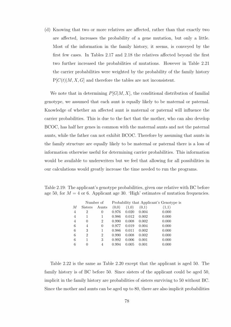
(d) Knowing that two or more relatives are affected, rather than that exactly two
are affected, increases the probability of a gene mutation, but only a little.
Most of the information in the family history, it seems, is conveyed by the
first few cases. In Tables 2.17 and 2.18 the relatives affected beyond the first
two further increased the probabilities of mutations. However in Table 2.21
the carrier probabilities were weighted by the probability of the family history
P[C(t)|M,X,G] and therefore the tables are not inconsistent.
We note that in determining P [G|M,X], the conditional distribution of familial
genotype, we assumed that each aunt is equally likely to be maternal or paternal.
Knowledge of whether an affected aunt is maternal or paternal will influence the
carrier probabilities. This is due to the fact that the mother, who can also develop
BCOC, has half her genes in common with the maternal aunts and not the paternal
aunts, while the father can not exhibit BCOC. Therefore by assuming that aunts in
the family structure are equally likely to be maternal or paternal there is a loss of
information otherwise useful for determining carrier probabilities. This information
would be available to underwriters but we feel that allowing for all possibilities in
our calculations would greatly increase the time needed to run the programs.
Table 2.19: The applicant’s genotype probabilities, given one relative with BC beforeage 50, for M = 4 or 6. Applicant age 30. ‘High’ estimates of mutation frequencies.
Number of Probability that Applicant’s Genotype isM Sisters Aunts (0,0) (1,0) (0,1) (1,1)4 2 0 0.976 0.020 0.004 0.0004 1 1 0.986 0.012 0.002 0.0004 0 2 0.990 0.008 0.002 0.0006 4 0 0.977 0.019 0.004 0.0006 3 1 0.986 0.011 0.002 0.0006 2 2 0.990 0.008 0.002 0.0006 1 3 0.992 0.006 0.001 0.0006 0 4 0.994 0.005 0.001 0.000
Table 2.22 is the same as Table 2.20 except that the applicant is aged 50. The
family history is of BC before 50. Since sisters of the applicant could be aged 50,
implicit in the family history are probabilities of sisters surviving to 50 without BC.
Since the mother and aunts can be aged up to 80, there are also implicit probabilities
78
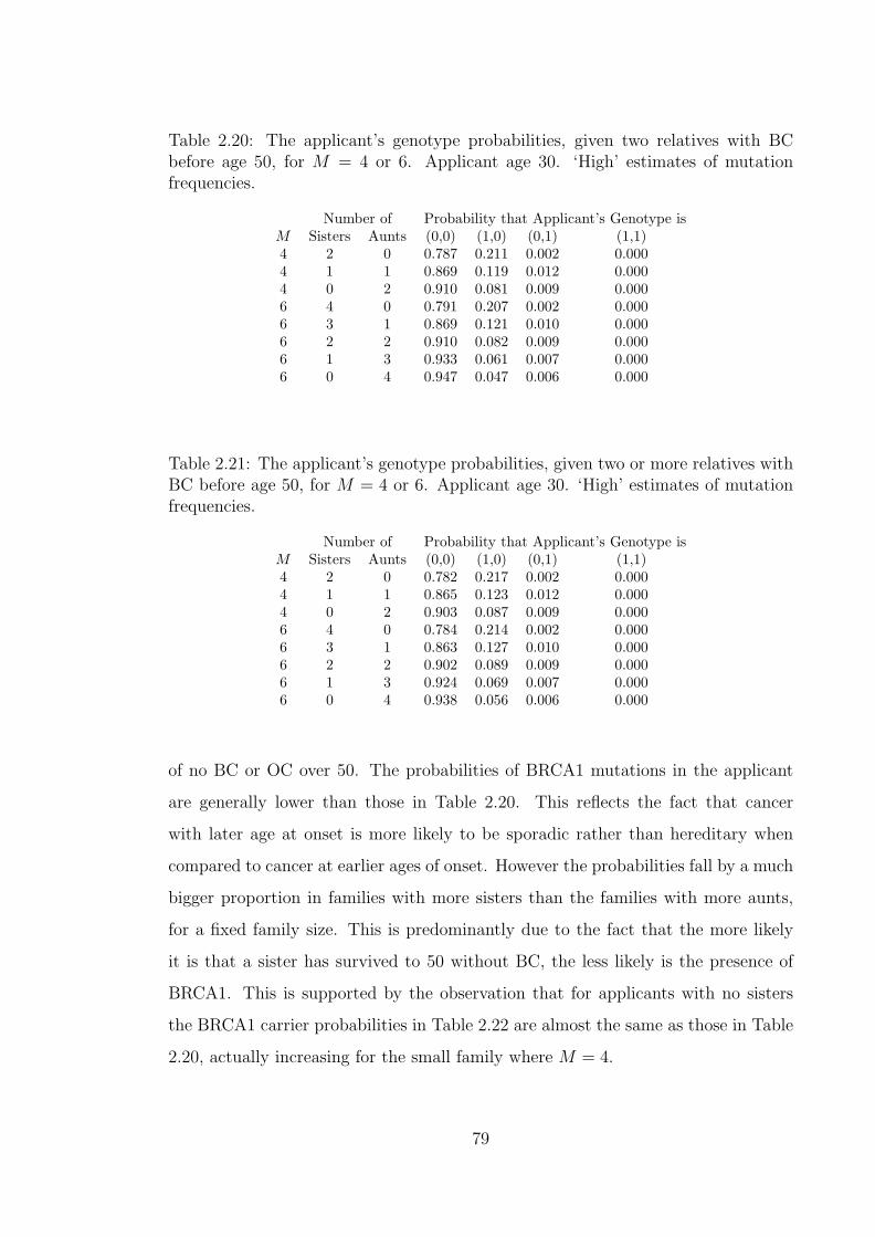
Table 2.20: The applicant’s genotype probabilities, given two relatives with BCbefore age 50, for M = 4 or 6. Applicant age 30. ‘High’ estimates of mutationfrequencies.
Number of Probability that Applicant’s Genotype isM Sisters Aunts (0,0) (1,0) (0,1) (1,1)4 2 0 0.787 0.211 0.002 0.0004 1 1 0.869 0.119 0.012 0.0004 0 2 0.910 0.081 0.009 0.0006 4 0 0.791 0.207 0.002 0.0006 3 1 0.869 0.121 0.010 0.0006 2 2 0.910 0.082 0.009 0.0006 1 3 0.933 0.061 0.007 0.0006 0 4 0.947 0.047 0.006 0.000
Table 2.21: The applicant’s genotype probabilities, given two or more relatives withBC before age 50, for M = 4 or 6. Applicant age 30. ‘High’ estimates of mutationfrequencies.
Number of Probability that Applicant’s Genotype isM Sisters Aunts (0,0) (1,0) (0,1) (1,1)4 2 0 0.782 0.217 0.002 0.0004 1 1 0.865 0.123 0.012 0.0004 0 2 0.903 0.087 0.009 0.0006 4 0 0.784 0.214 0.002 0.0006 3 1 0.863 0.127 0.010 0.0006 2 2 0.902 0.089 0.009 0.0006 1 3 0.924 0.069 0.007 0.0006 0 4 0.938 0.056 0.006 0.000
of no BC or OC over 50. The probabilities of BRCA1 mutations in the applicant
are generally lower than those in Table 2.20. This reflects the fact that cancer
with later age at onset is more likely to be sporadic rather than hereditary when
compared to cancer at earlier ages of onset. However the probabilities fall by a much
bigger proportion in families with more sisters than the families with more aunts,
for a fixed family size. This is predominantly due to the fact that the more likely
it is that a sister has survived to 50 without BC, the less likely is the presence of
BRCA1. This is supported by the observation that for applicants with no sisters
the BRCA1 carrier probabilities in Table 2.22 are almost the same as those in Table
2.20, actually increasing for the small family where M = 4.
79

For BRCA2, carrier probabilities are generally lower in Table 2.22 than in Table
2.20 but the effect of the family structure on the proportional differences is the
reverse of that of BRCA1. For fixed family size the higher the number of aunts,
the lower the proportional fall in the probabilities from Table 2.20 to Table 2.22.
This is not unexpected since for the aunt and mother the change in life histories is
expected at ages 50 and above and these ages have a higher influence on BRCA2
probabilities.
An interesting case corresponds to the points (b) discussed above. We had the
case where the implication that a sister had BC before 50 meant very low proba-
bilities of BRCA2. In Table 2.22, alongside that same implication, the event that
a sister survived BC before 50 greatly reduces the chance of BRCA1 and also the
event that there are two relatives affected points to either BRCA1 or BRCA2. The
result is a significant increase in the BRCA2 probabilities of about 8 times.
Table 2.22: The applicant’s genotype probabilities, given two relatives with BCbefore age 50, for M = 4 or 6. Applicant age 50. ‘High’ estimates of mutationfrequencies.
Number of Probability that Applicant’s Genotype isM Sisters Aunts (0,0) (1,0) (0,1) (1,1)4 2 0 0.840 0.144 0.016 0.0004 1 1 0.874 0.114 0.012 0.0004 0 2 0.910 0.082 0.008 0.0006 4 0 0.904 0.082 0.013 0.0006 3 1 0.916 0.074 0.010 0.0006 2 2 0.927 0.065 0.008 0.0006 1 3 0.939 0.055 0.006 0.0006 0 4 0.950 0.046 0.004 0.000
In Table 2.23 we show our first example of the effect of using ‘low’ mutation
estimates on carrier probabilities. We recall that the low mutations frequencies are
shown in Table 2.11 and are based on a BRCA1 mutation frequency of 0.000450 and
a BRCA2 mutation frequency of 0.000165. The case considered is the same as that
in Table 2.20 and the results show a significant fall in the carrier probabilities for
both BRCA1 and BRCA2. Any insurance risk assessment based on genotypes will
need to be based on good estimates of gene frequencies.
80
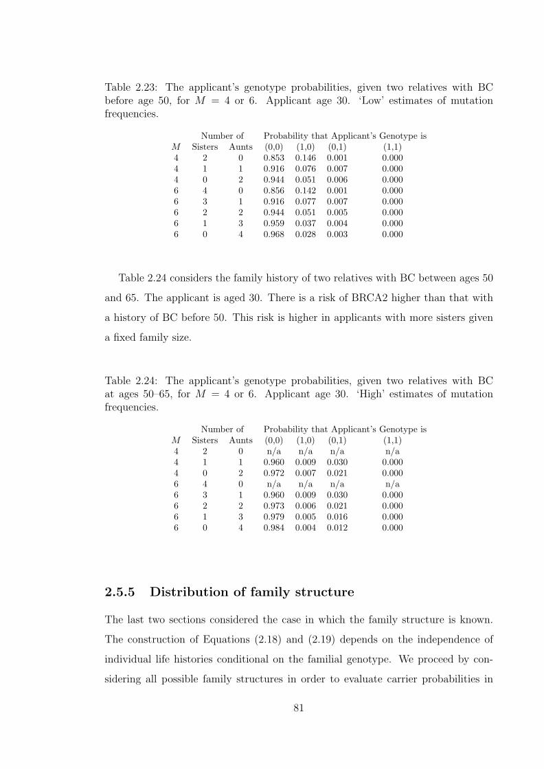
Table 2.23: The applicant’s genotype probabilities, given two relatives with BCbefore age 50, for M = 4 or 6. Applicant age 30. ‘Low’ estimates of mutationfrequencies.
Number of Probability that Applicant’s Genotype isM Sisters Aunts (0,0) (1,0) (0,1) (1,1)4 2 0 0.853 0.146 0.001 0.0004 1 1 0.916 0.076 0.007 0.0004 0 2 0.944 0.051 0.006 0.0006 4 0 0.856 0.142 0.001 0.0006 3 1 0.916 0.077 0.007 0.0006 2 2 0.944 0.051 0.005 0.0006 1 3 0.959 0.037 0.004 0.0006 0 4 0.968 0.028 0.003 0.000
Table 2.24 considers the family history of two relatives with BC between ages 50
and 65. The applicant is aged 30. There is a risk of BRCA2 higher than that with
a history of BC before 50. This risk is higher in applicants with more sisters given
a fixed family size.
Table 2.24: The applicant’s genotype probabilities, given two relatives with BCat ages 50–65, for M = 4 or 6. Applicant age 30. ‘High’ estimates of mutationfrequencies.
Number of Probability that Applicant’s Genotype isM Sisters Aunts (0,0) (1,0) (0,1) (1,1)4 2 0 n/a n/a n/a n/a4 1 1 0.960 0.009 0.030 0.0004 0 2 0.972 0.007 0.021 0.0006 4 0 n/a n/a n/a n/a6 3 1 0.960 0.009 0.030 0.0006 2 2 0.973 0.006 0.021 0.0006 1 3 0.979 0.005 0.016 0.0006 0 4 0.984 0.004 0.012 0.000
2.5.5 Distribution of family structure
The last two sections considered the case in which the family structure is known.
The construction of Equations (2.18) and (2.19) depends on the independence of
individual life histories conditional on the familial genotype. We proceed by con-
sidering all possible family structures in order to evaluate carrier probabilities in
81

cases where the family structure is unknown. The size M and ages X may both be
unknown or the size may be known while the ages are unknown. If the family struc-
ture is not known completely then the family history cannot be known completely.
Summary definitions of family history, as used in underwriting, may state
(a) the total number of relatives who have had BC or OC ever,
(b) total number of relatives with BC or OC with age-groups of onset.
(c) minimum number of relatives with BC or OC ever,
(d) minimum number of relatives with BC or OC with age-groups of onset.
The distribution of family structures is required in order to compute carrier prob-
abilities with unknown family structures. We define the random variables
Dm = Number of daughters borne by the applicant’s mother
Dmm = Number of daughters borne by the applicant’s maternal grandmother
Dfm = Number of daughters borne by the applicant’s paternal grandmother
Sfm = Number of sons borne by the applicant’s paternal grandmother.
Since the applicant always has a mother, finding the probability distribution of
the family structure is equivalent to establishing the probability that the applicant
has s sisters and a aunts, for all possible values of s and a. We note that
(a) for the applicant to have s sisters then Dm = s + 1,
(b) the applicant has a mother, therefore Dmm > 0, and
(c) the applicant has a father, therefore Sfm > 0.
The probability that the applicant has s sisters and a aunts is
P[Dm = s + 1|Dm > 0]P[Dmm + Dfm = a + 1|Dmm > 0, Sfm > 0]
We let am be the number of maternal aunts and af the number of paternal aunts.
Therefore a = am+af and the applicant will have am maternal aunts if Dmm = am+1
and have af paternal aunts if Dfm = af . Using these equations, and the fact that
Dmm and Dfm are conditionally independent given Dmm > 0 and Sfm > 0
82

P[Dm = s + 1|Dm > 0]P[Dmm + Dfm = a + 1|Dmm > 0, Sfm > 0]
= P[Dm = s + 1|Dm > 0]
(am=a∑am=0
P[Dmm = am + 1, Dfm = a− am|Dmm > 0, Sfm > 0]
)
= P[Dm = s + 1|Dm > 0]
(am=a∑am=0
P[Dmm = am + 1|Dmm > 0, Sfm > 0]
×P[Dfm = a− am|Dmm > 0, Sfm > 0])
= P[Dm = s + 1|Dm > 0]
(am=a∑am=0
P[Dmm = am + 1|Dmm > 0]P[Dfm = a− am|Sfm > 0]
)
=P[Dm = s + 1]
P[Dm > 0]
(am=a∑am=0
P[Dmm = am + 1]P[Dmm > 0]
P[Dfm = a− am, Sfm > 0]P[Sfm > 0]
). (2.21)
To establish the expressions in the equation we let D be the total number of
daughters and S the total number of sons born to a given woman, and C = D + S
the total number of her children. We assume that the probability that a child born
is male is 1.06/2.06 (Coleman and Salt (1992)). For a woman with c children the
probability that exactly d of them are daughters is(c
d
)(1
2.06
)d (1.06
2.06
)c−d
.
Summing over all possible number of children, weighted by the probability dis-
tribution of the number of children, P (C = c), we get
P[D = d] =c=∞∑c=d
P[C = c]
(c
d
) (1
2.06
)d (1.06
2.06
)c−d
. (2.22)
The probability that a woman has d daughters and at least one son is
P[D = d, S > 0] =c=∞∑
c=d+1
P[C = c]
(c
d
) (1
2.06
)d (1.06
2.06
)c−d
(2.23)
and the probability that she has at least one son is
P[S > 0] = 1−c=∞∑c=0
P[C = c]
(1
2.06
)c
. (2.24)
In practice the number of children a women can have will be limited and there-
fore D and S will not be independent. Equations (2.22) to (2.24) are substituted in
Equation (2.21) to get P [M,X]. However we note that the distribution of number
83

of children borne will not be the same for the applicant’s mother and of the grand-
mothers. Family sizes have changed significantly over time. Since our examples are
mostly for applicants aged 30, we should consider mothers born in about 1940 and
grandmothers born in about 1910. For the distribution of family size applicable to
the mother’s generation we will use results of interviews with women in the Gen-
eral Household Survey of 1987. These are given by Shaw (1990) and in Table 2.25
we give the values for women born between 1930 and 1944. For the 1940–44 birth
cohort, the values are based on expected final number of children since the women
were still of child bearing age at the time of the interviews.
Table 2.25: Distribution of final or expected numbers of children born to womenborn in England and Wales in 1930–44. (Source: Shaw (1990).)
Number of children AverageBirth cohort 0 1 2 3 ≥ 4 Family Size
% % % % %1930–34 13 13 29 22 23 2.491935–39 10 11 35 24 20 2.491940–44 9 13 40 20 18 2.38
The fertility report O.P.C.S. (1983) gives the distribution of family size for women
by year of marriage. Table 2.26 shows the distribution for women married in 1931
to 1935 and those married in 1961 to 1965. The distributions are based on data
from 1.17 million women (1931 to 1935) and 1.46 million women (1961 to 1965)
aged below 45.
Table 2.26: Distribution of numbers of children according to year of mother’s mar-riage, England and Wales. (Source: O.P.C.S. (1983).)
Number of childrenYear of Marriage 0 1 2 3 4 5 6 ≥ 7
% % % % % % % %1931–35 17.5 27.0 26.6 14.3 7.0 3.50 1.80 2.301961–65 11.3 20.5 44.4 17.5 4.8 1.10 0.30 0.10
84

For the purposes of our calculations, the following points will apply with respect
to the values in Tables 2.25 and 2.26.
(a) Due to the way the data are given, we restrict C to C ≤ 7.
(b) We take the first line of Table 2.26 to represent the distribution of C in respect
of the applicant’s grandmothers.
(c) We take the third line of Table 2.25 to represent the distribution of C in respect
of the applicant’s mother. We note that even though these values are based
on a much smaller sample than those in Table 2.26, they are obtained 16 years
later. However we need to split the 18% of women with four or more children.
From Table 2.26, for women in the marriage years 1961–65, the 6.3% of women
with 4 or more children are in the ratios
1.000 : 0.2292 : 0.0625 : 0.0208
of having 4, 5, 6 and 7 or more children respectively. Applying these ratios to
the 18% of women, we get 13.7%, 3.14%, 0.86% and 0.29% of women with 4, 5,
6 and 7 children respectively.
Using these values of P[C = c], in Equations (2.22) to (2.24), Equation (2.21)
gives the distribution given in Table 2.27.
85
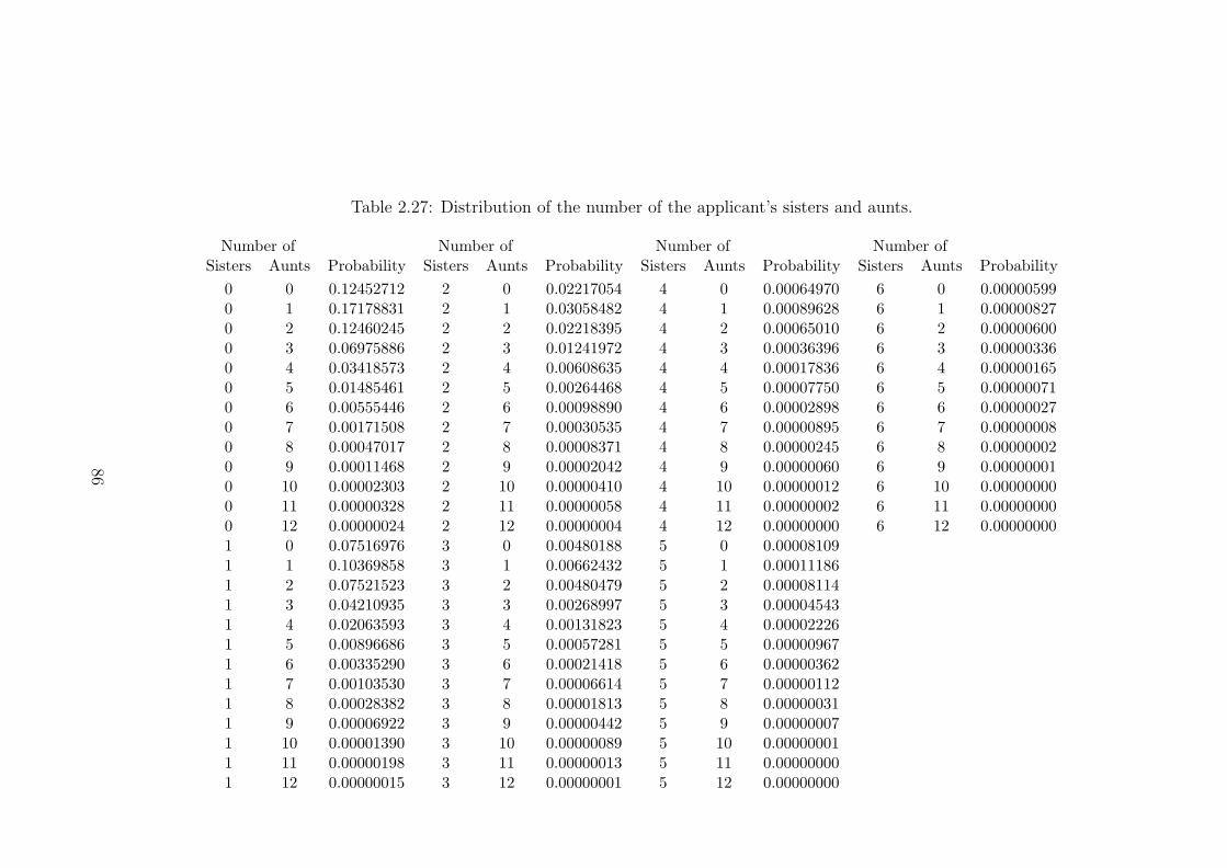
Table 2.27: Distribution of the number of the applicant’s sisters and aunts.
Number of Number of Number of Number ofSisters Aunts Probability Sisters Aunts Probability Sisters Aunts Probability Sisters Aunts Probability
0 0 0.12452712 2 0 0.02217054 4 0 0.00064970 6 0 0.000005990 1 0.17178831 2 1 0.03058482 4 1 0.00089628 6 1 0.000008270 2 0.12460245 2 2 0.02218395 4 2 0.00065010 6 2 0.000006000 3 0.06975886 2 3 0.01241972 4 3 0.00036396 6 3 0.000003360 4 0.03418573 2 4 0.00608635 4 4 0.00017836 6 4 0.000001650 5 0.01485461 2 5 0.00264468 4 5 0.00007750 6 5 0.000000710 6 0.00555446 2 6 0.00098890 4 6 0.00002898 6 6 0.000000270 7 0.00171508 2 7 0.00030535 4 7 0.00000895 6 7 0.000000080 8 0.00047017 2 8 0.00008371 4 8 0.00000245 6 8 0.000000020 9 0.00011468 2 9 0.00002042 4 9 0.00000060 6 9 0.000000010 10 0.00002303 2 10 0.00000410 4 10 0.00000012 6 10 0.000000000 11 0.00000328 2 11 0.00000058 4 11 0.00000002 6 11 0.000000000 12 0.00000024 2 12 0.00000004 4 12 0.00000000 6 12 0.000000001 0 0.07516976 3 0 0.00480188 5 0 0.000081091 1 0.10369858 3 1 0.00662432 5 1 0.000111861 2 0.07521523 3 2 0.00480479 5 2 0.000081141 3 0.04210935 3 3 0.00268997 5 3 0.000045431 4 0.02063593 3 4 0.00131823 5 4 0.000022261 5 0.00896686 3 5 0.00057281 5 5 0.000009671 6 0.00335290 3 6 0.00021418 5 6 0.000003621 7 0.00103530 3 7 0.00006614 5 7 0.000001121 8 0.00028382 3 8 0.00001813 5 8 0.000000311 9 0.00006922 3 9 0.00000442 5 9 0.000000071 10 0.00001390 3 10 0.00000089 5 10 0.000000011 11 0.00000198 3 11 0.00000013 5 11 0.000000001 12 0.00000015 3 12 0.00000001 5 12 0.00000000
86
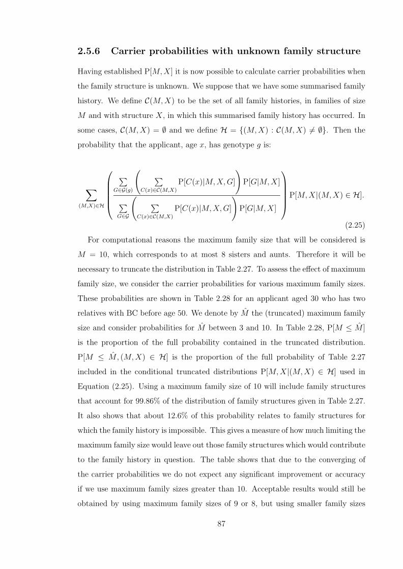
2.5.6 Carrier probabilities with unknown family structure
Having established P[M,X] it is now possible to calculate carrier probabilities when
the family structure is unknown. We suppose that we have some summarised family
history. We define C(M,X) to be the set of all family histories, in families of size
M and with structure X, in which this summarised family history has occurred. In
some cases, C(M,X) = ∅ and we define H = {(M,X) : C(M,X) 6= ∅}. Then the
probability that the applicant, age x, has genotype g is:
∑(M,X)∈H
∑G∈G(g)
( ∑C(x)∈C(M,X)
P[C(x)|M,X,G]
)P[G|M,X]
∑G∈G
( ∑C(x)∈C(M,X)
P[C(x)|M,X,G]
)P[G|M,X]
P[M,X|(M,X) ∈ H].
(2.25)
For computational reasons the maximum family size that will be considered is
M = 10, which corresponds to at most 8 sisters and aunts. Therefore it will be
necessary to truncate the distribution in Table 2.27. To assess the effect of maximum
family size, we consider the carrier probabilities for various maximum family sizes.
These probabilities are shown in Table 2.28 for an applicant aged 30 who has two
relatives with BC before age 50. We denote by M the (truncated) maximum family
size and consider probabilities for M between 3 and 10. In Table 2.28, P[M ≤ M ]
is the proportion of the full probability contained in the truncated distribution.
P[M ≤ M, (M,X) ∈ H] is the proportion of the full probability of Table 2.27
included in the conditional truncated distributions P[M,X|(M,X) ∈ H] used in
Equation (2.25). Using a maximum family size of 10 will include family structures
that account for 99.86% of the distribution of family structures given in Table 2.27.
It also shows that about 12.6% of this probability relates to family structures for
which the family history is impossible. This gives a measure of how much limiting the
maximum family size would leave out those family structures which would contribute
to the family history in question. The table shows that due to the converging of
the carrier probabilities we do not expect any significant improvement or accuracy
if we use maximum family sizes greater than 10. Acceptable results would still be
obtained by using maximum family sizes of 9 or 8, but using smaller family sizes
87
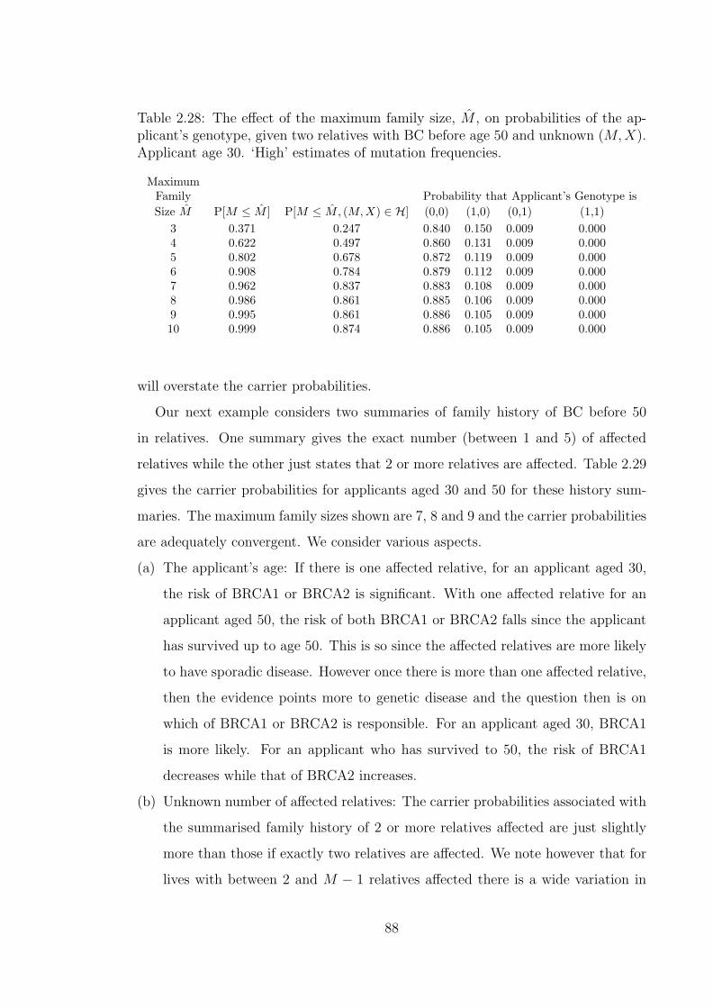
Table 2.28: The effect of the maximum family size, M , on probabilities of the ap-plicant’s genotype, given two relatives with BC before age 50 and unknown (M,X).Applicant age 30. ‘High’ estimates of mutation frequencies.
MaximumFamily Probability that Applicant’s Genotype isSize M P[M ≤ M ] P[M ≤ M, (M,X) ∈ H] (0,0) (1,0) (0,1) (1,1)
3 0.371 0.247 0.840 0.150 0.009 0.0004 0.622 0.497 0.860 0.131 0.009 0.0005 0.802 0.678 0.872 0.119 0.009 0.0006 0.908 0.784 0.879 0.112 0.009 0.0007 0.962 0.837 0.883 0.108 0.009 0.0008 0.986 0.861 0.885 0.106 0.009 0.0009 0.995 0.861 0.886 0.105 0.009 0.00010 0.999 0.874 0.886 0.105 0.009 0.000
will overstate the carrier probabilities.
Our next example considers two summaries of family history of BC before 50
in relatives. One summary gives the exact number (between 1 and 5) of affected
relatives while the other just states that 2 or more relatives are affected. Table 2.29
gives the carrier probabilities for applicants aged 30 and 50 for these history sum-
maries. The maximum family sizes shown are 7, 8 and 9 and the carrier probabilities
are adequately convergent. We consider various aspects.
(a) The applicant’s age: If there is one affected relative, for an applicant aged 30,
the risk of BRCA1 or BRCA2 is significant. With one affected relative for an
applicant aged 50, the risk of both BRCA1 or BRCA2 falls since the applicant
has survived up to age 50. This is so since the affected relatives are more likely
to have sporadic disease. However once there is more than one affected relative,
then the evidence points more to genetic disease and the question then is on
which of BRCA1 or BRCA2 is responsible. For an applicant aged 30, BRCA1
is more likely. For an applicant who has survived to 50, the risk of BRCA1
decreases while that of BRCA2 increases.
(b) Unknown number of affected relatives: The carrier probabilities associated with
the summarised family history of 2 or more relatives affected are just slightly
more than those if exactly two relatives are affected. We note however that for
lives with between 2 and M − 1 relatives affected there is a wide variation in
88

Table 2.29: The effect of the family history (BC before age 50 only) and maximumfamily size, M , on probabilities of the applicant’s genotype, unknown (M,X). ‘High’estimates of mutation frequencies.
Number of MaximumApplicant’s Relatives with Family Probability that Applicant’s Genotype is
Age BC Before 50 Size M (0,0) (1,0) (0,1) (1,1)30 1 7 0.985 0.012 0.002 0.00030 1 8 0.985 0.012 0.002 0.00030 1 9 0.986 0.012 0.002 0.00030 2 7 0.883 0.108 0.009 0.00030 2 8 0.885 0.106 0.009 0.00030 2 9 0.886 0.105 0.009 0.00030 3 7 0.655 0.332 0.012 0.00030 3 8 0.660 0.327 0.012 0.00030 3 9 0.662 0.325 0.012 0.00030 4 7 0.544 0.447 0.008 0.00130 4 8 0.550 0.442 0.008 0.00130 4 9 0.552 0.439 0.008 0.00130 5 7 0.515 0.480 0.004 0.00130 5 8 0.520 0.474 0.005 0.00130 5 9 0.523 0.471 0.005 0.00130 ≥ 2 7 0.880 0.111 0.009 0.00030 ≥ 2 8 0.882 0.109 0.009 0.00030 ≥ 2 9 0.883 0.109 0.009 0.00050 1 7 0.988 0.010 0.002 0.00050 1 8 0.988 0.010 0.002 0.00050 1 9 0.988 0.010 0.002 0.00050 2 7 0.892 0.097 0.010 0.00050 2 8 0.894 0.096 0.010 0.00050 2 9 0.895 0.095 0.010 0.00050 3 7 0.658 0.323 0.018 0.00050 3 8 0.663 0.319 0.018 0.00050 3 9 0.666 0.316 0.018 0.00050 4 7 0.542 0.444 0.014 0.00150 4 8 0.545 0.440 0.014 0.00150 4 9 0.547 0.439 0.013 0.00150 5 7 0.513 0.477 0.009 0.00150 5 8 0.517 0.474 0.009 0.00150 5 9 0.519 0.472 0.009 0.00150 ≥ 2 7 0.886 0.104 0.010 0.00050 ≥ 2 8 0.888 0.102 0.010 0.00050 ≥ 2 9 0.888 0.101 0.010 0.000
89
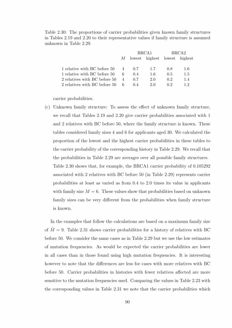
Table 2.30: The proportions of carrier probabilities given known family structuresin Tables 2.19 and 2.20 to their representative values if family structure is assumedunknown in Table 2.29.
BRCA1 BRCA2M lowest highest lowest highest
1 relative with BC before 50 4 0.7 1.7 0.8 1.61 relative with BC before 50 6 0.4 1.6 0.5 1.52 relatives with BC before 50 4 0.7 2.0 0.2 1.42 relatives with BC before 50 6 0.4 2.0 0.2 1.2
carrier probabilities.
(c) Unknown family structure: To assess the effect of unknown family structure,
we recall that Tables 2.19 and 2.20 give carrier probabilities associated with 1
and 2 relatives with BC before 50, where the family structure is known. These
tables considered family sizes 4 and 6 for applicants aged 30. We calculated the
proportion of the lowest and the highest carrier probabilities in these tables to
the carrier probability of the corresponding history in Table 2.29. We recall that
the probabilities in Table 2.29 are averages over all possible family structures.
Table 2.30 shows that, for example, the BRCA1 carrier probability of 0.105292
associated with 2 relatives with BC before 50 (in Table 2.29) represents carrier
probabilities at least as varied as from 0.4 to 2.0 times its value in applicants
with family size M = 6. These values show that probabilities based on unknown
family sizes can be very different from the probabilities when family structure
is known.
In the examples that follow the calculations are based on a maximum family size
of M = 9. Table 2.31 shows carrier probabilities for a history of relatives with BC
before 50. We consider the same cases as in Table 2.29 but we use the low estimates
of mutation frequencies. As would be expected the carrier probabilities are lower
in all cases than in those found using high mutation frequencies. It is interesting
however to note that the differences are less for cases with more relatives with BC
before 50. Carrier probabilities in histories with fewer relatives affected are more
sensitive to the mutation frequencies used. Comparing the values in Table 2.23 with
the corresponding values in Table 2.31 we note that the carrier probabilities which
90

Table 2.31: The effect of the family history (BC before age 50) on probabilities ofthe applicant’s genotype, unknown (M,X). Maximum family size M = 9. ‘Low’estimates of mutation frequencies.
Number ofApplicant’s Relatives with Probability that Applicant’s Genotype is
Age BC Before 50 (0,0) (1,0) (0,1) (1,1)30 1 0.992 0.007 0.001 0.00030 2 0.927 0.068 0.005 0.00030 3 0.714 0.276 0.010 0.00030 4 0.566 0.426 0.007 0.00030 5 0.528 0.468 0.004 0.00130 ≥ 2 0.924 0.070 0.005 0.00050 1 0.993 0.006 0.001 0.00050 2 0.933 0.060 0.006 0.00050 3 0.721 0.264 0.014 0.00050 4 0.563 0.425 0.012 0.00050 5 0.523 0.469 0.008 0.00150 ≥ 2 0.929 0.065 0.006 0.000
do not take into account family structure are representing a wide range of carrier
probabilities. The magnitude of variation is similar to that shown in Table 2.30.
In Tables 2.32 and 2.33 we consider the probabilities associated with BC history
in the ages 50–65. We recall from our discussion of Table 2.17 that BC in this age
range gives high probabilities of BRCA2, which are even higher than the BRCA1
probabilities. This feature is present in both Tables 2.32 and 2.33. The probabilities
are much higher when more relatives are affected. In a way similar to the history
of BC before 50, the mutation frequencies have more impact when fewer relatives
are affected. The effect of unknown family structure on the carrier probabilities is
seen when we compare values in Table 2.24 to corresponding values in Table 2.32.
Probabilities corresponding to a known family structure are significantly different
from those based on unknown family structures.
Tables 2.34 to 2.37 consider history of OC below age 50 and OC between ages
50 and 65. We note that OC before 50 very much points to the presence of BRCA1
mutations. As the number of relatives affected increases, the probabilities of BRCA1
increase significantly while the BRCA2 probabilities fall. For 4 or more relatives
affected, the BRCA2 probabilities fall below population frequencies. For cases where
OC is between 50 and 65 the carrier probabilities of BRCA1 are lower than for OC
91

Table 2.32: The effect of the family history (BC at ages 50–65) on probabilities ofthe applicant’s genotype, unknown (M,X). Maximum family size M = 9. ‘High’estimates of mutation frequencies.
Number ofApplicant’s Relatives with Probability that Applicant’s Genotype is
Age BC at 50–65 (0,0) (1,0) (0,1) (1,1)30 1 0.994 0.003 0.003 0.00030 2 0.970 0.007 0.023 0.00030 3 0.882 0.013 0.105 0.00030 4 0.712 0.013 0.275 0.00030 5 0.597 0.008 0.394 0.00130 ≥ 2 0.969 0.007 0.023 0.00050 1 0.995 0.002 0.003 0.00050 2 0.980 0.004 0.016 0.00050 3 0.922 0.007 0.071 0.00050 4 0.780 0.008 0.211 0.00050 5 0.640 0.006 0.354 0.00150 ≥ 2 0.979 0.004 0.016 0.000
Table 2.33: The effect of the family history (BC at ages 50–65) on probabilities ofthe applicant’s genotype, unknown (M,X). Maximum family size M = 9. ‘Low’estimates of mutation frequencies.
Number ofApplicant’s Relatives with Probability that Applicant’s Genotype is
Age BC at 50–65 (0,0) (1,0) (0,1) (1,1)30 1 0.996 0.002 0.002 0.00030 2 0.983 0.004 0.013 0.00030 3 0.925 0.008 0.066 0.00030 4 0.772 0.010 0.217 0.00030 5 0.624 0.007 0.369 0.00030 ≥ 2 0.982 0.004 0.013 0.00050 1 0.997 0.001 0.001 0.00050 2 0.989 0.003 0.009 0.00050 3 0.953 0.004 0.043 0.00050 4 0.841 0.006 0.153 0.00050 5 0.681 0.005 0.314 0.00050 ≥ 2 0.988 0.003 0.009 0.000
92

before 50 while BRCA2 probabilities are higher. The total probability of having
some mutation is lower for a history of OC between 50 and 65 than for OC before
50.
Table 2.34: The effect of the family history (OC before age 50) on probabilities ofthe applicant’s genotype, unknown (M,X). Maximum family size M = 9. ‘High’estimates of mutation frequencies.
Number ofApplicant’s Relatives with Probability that Applicant’s Genotype is
Age OC Before 50 (0,0) (1,0) (0,1) (1,1)30 1 0.978 0.020 0.001 0.00030 2 0.804 0.193 0.002 0.00030 3 0.584 0.415 0.001 0.00030 4 0.531 0.468 0.001 0.00030 5 0.515 0.484 0.000 0.00030 ≥ 2 0.803 0.194 0.002 0.00050 1 0.982 0.017 0.001 0.00050 2 0.801 0.196 0.003 0.00050 3 0.572 0.427 0.001 0.00050 4 0.524 0.475 0.001 0.00050 5 0.511 0.488 0.000 0.00050 ≥ 2 0.798 0.199 0.003 0.000
2.5.7 Effect of lower BRCA1 and BRCA2 penetrance
In Table 2.7 we showed a number of estimates of the penetrance of BRCA1. It
shows that there has been wide variation in the estimates published. The confidence
intervals of the estimates are quite wide, so that these values can not be taken as very
reliable. These penetrance estimates were largely based on studies of women selected
for their particularly strong family history of BC or OC. We feel that these estimates
are more likely to overestimate than underestimate the penetrance. In Tables 2.38 to
2.40 we consider the effect that reducing penetrance has on the carrier probabilities.
We consider two scenarios in which we reduce the excess incidence rates of BC or OC
in mutation carriers over the population BC or OC incidence rates to 50% and 25% of
the values we have used so far. This means that we maintain the general shape of the
incidence rates in the parameterisation of Section 2.5.2. By considering reductions
in the excess incidence rates rather than the reduction in absolute incidence rates,
we ensure that the ordering of the incidence rates for sporadic, BRCA1 and BRCA2
93

Table 2.35: The effect of the family history (OC before age 50) on probabilities ofthe applicant’s genotype, unknown (M,X). Maximum family size M = 9. ‘Low’estimates of mutation frequencies.
Number ofApplicant’s Relatives with Probability that Applicant’s Genotype is
Age OC Before 50 (0,0) (1,0) (0,1) (1,1)30 1 0.987 0.012 0.001 0.00030 2 0.862 0.137 0.002 0.00030 3 0.610 0.390 0.001 0.00030 4 0.535 0.464 0.000 0.00030 5 0.518 0.481 0.000 0.00030 ≥ 2 0.861 0.138 0.002 0.00050 1 0.989 0.010 0.001 0.00050 2 0.858 0.140 0.002 0.00050 3 0.595 0.404 0.001 0.00050 4 0.527 0.473 0.000 0.00050 5 0.513 0.486 0.000 0.00050 ≥ 2 0.856 0.143 0.002 0.000
disease is maintained. Reducing the excess incidence rates to 50% and 25% will
correspond to a reduction in BRCA1 penetrance for BC at age 80 to about 60% and
40% respectively. These levels for the penetrance are in line with the penetrance
estimates obtained from recent studies like Antoniou et al. (2000) which gives a
penetrance for BC of 45% by age 70 ( see Table 2.7).
In Tables 2.38 and 2.39 we assume that the family structure is known with sizes
M = 4 and M = 6. The applicant is aged 30, and we consider the history of one
and two relatives with BC before age 50. In all cases the BRCA1 carrier probabil-
ities are significantly reduced. The reduction is more marked in the higher carrier
probabilities. This means there is more reduction in carrier probabilities given two
relatives affected than given one relative affected, and more reduction given more
sisters in the family structure than fewer sisters. For a reduction in excess risk to
50% of current values, the BRCA1 carrier probabilities fall by up to a factor of 2
while for a reduction to 25% of current excess risk values the probabilities fall by
up to a factor of 5.
The BRCA2 carrier probabilities fall significantly in most of the cases. However,
in the cases where there are no aunts, and two relatives with BC before 50, that is
the cases when it is implied that a sister has had BC before 50, the lowering of the
94
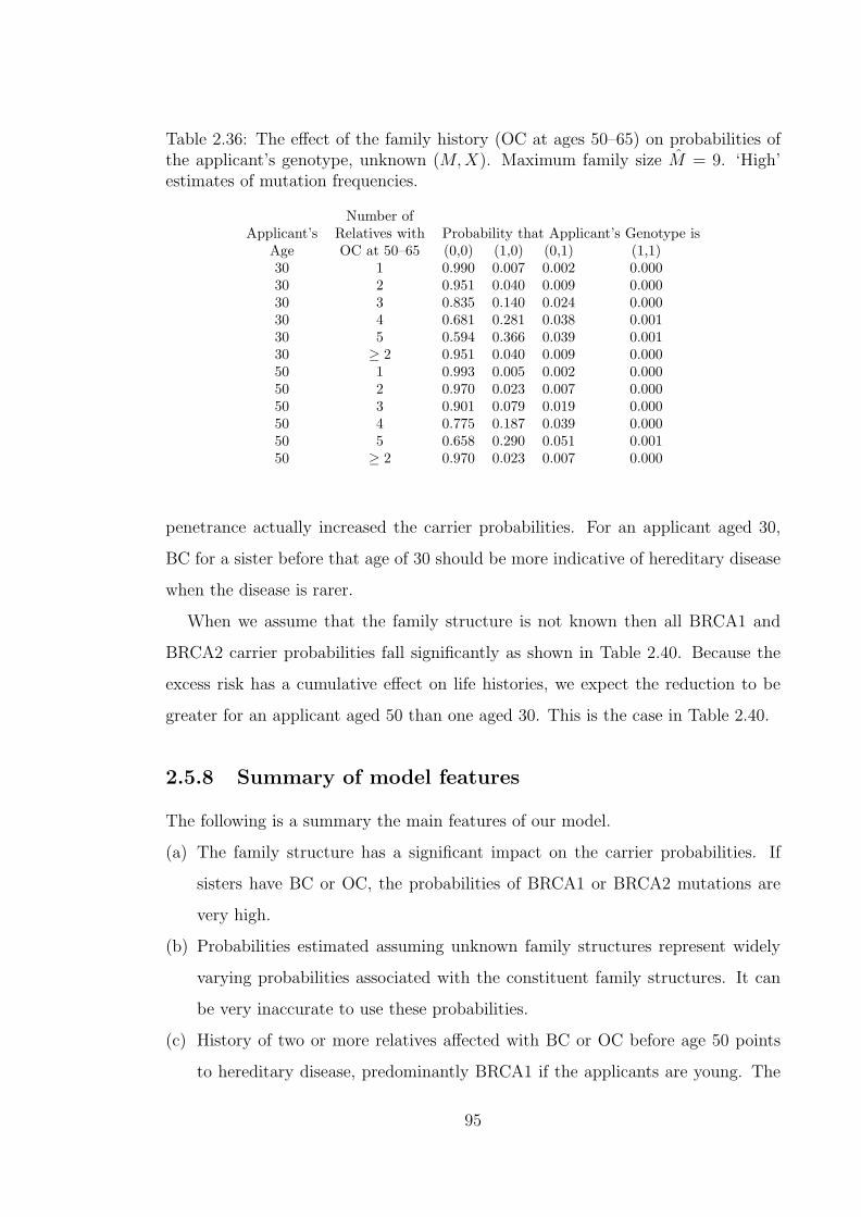
Table 2.36: The effect of the family history (OC at ages 50–65) on probabilities ofthe applicant’s genotype, unknown (M,X). Maximum family size M = 9. ‘High’estimates of mutation frequencies.
Number ofApplicant’s Relatives with Probability that Applicant’s Genotype is
Age OC at 50–65 (0,0) (1,0) (0,1) (1,1)30 1 0.990 0.007 0.002 0.00030 2 0.951 0.040 0.009 0.00030 3 0.835 0.140 0.024 0.00030 4 0.681 0.281 0.038 0.00130 5 0.594 0.366 0.039 0.00130 ≥ 2 0.951 0.040 0.009 0.00050 1 0.993 0.005 0.002 0.00050 2 0.970 0.023 0.007 0.00050 3 0.901 0.079 0.019 0.00050 4 0.775 0.187 0.039 0.00050 5 0.658 0.290 0.051 0.00150 ≥ 2 0.970 0.023 0.007 0.000
penetrance actually increased the carrier probabilities. For an applicant aged 30,
BC for a sister before that age of 30 should be more indicative of hereditary disease
when the disease is rarer.
When we assume that the family structure is not known then all BRCA1 and
BRCA2 carrier probabilities fall significantly as shown in Table 2.40. Because the
excess risk has a cumulative effect on life histories, we expect the reduction to be
greater for an applicant aged 50 than one aged 30. This is the case in Table 2.40.
2.5.8 Summary of model features
The following is a summary the main features of our model.
(a) The family structure has a significant impact on the carrier probabilities. If
sisters have BC or OC, the probabilities of BRCA1 or BRCA2 mutations are
very high.
(b) Probabilities estimated assuming unknown family structures represent widely
varying probabilities associated with the constituent family structures. It can
be very inaccurate to use these probabilities.
(c) History of two or more relatives affected with BC or OC before age 50 points
to hereditary disease, predominantly BRCA1 if the applicants are young. The
95
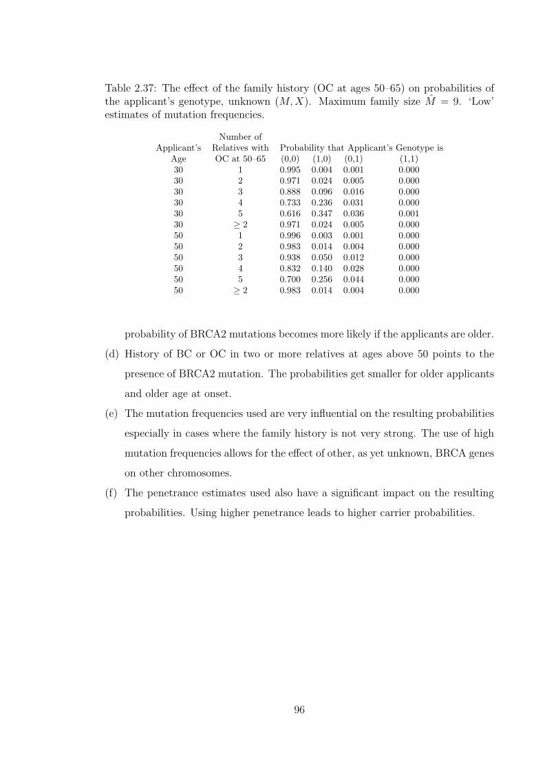
Table 2.37: The effect of the family history (OC at ages 50–65) on probabilities ofthe applicant’s genotype, unknown (M,X). Maximum family size M = 9. ‘Low’estimates of mutation frequencies.
Number ofApplicant’s Relatives with Probability that Applicant’s Genotype is
Age OC at 50–65 (0,0) (1,0) (0,1) (1,1)30 1 0.995 0.004 0.001 0.00030 2 0.971 0.024 0.005 0.00030 3 0.888 0.096 0.016 0.00030 4 0.733 0.236 0.031 0.00030 5 0.616 0.347 0.036 0.00130 ≥ 2 0.971 0.024 0.005 0.00050 1 0.996 0.003 0.001 0.00050 2 0.983 0.014 0.004 0.00050 3 0.938 0.050 0.012 0.00050 4 0.832 0.140 0.028 0.00050 5 0.700 0.256 0.044 0.00050 ≥ 2 0.983 0.014 0.004 0.000
probability of BRCA2 mutations becomes more likely if the applicants are older.
(d) History of BC or OC in two or more relatives at ages above 50 points to the
presence of BRCA2 mutation. The probabilities get smaller for older applicants
and older age at onset.
(e) The mutation frequencies used are very influential on the resulting probabilities
especially in cases where the family history is not very strong. The use of high
mutation frequencies allows for the effect of other, as yet unknown, BRCA genes
on other chromosomes.
(f) The penetrance estimates used also have a significant impact on the resulting
probabilities. Using higher penetrance leads to higher carrier probabilities.
96
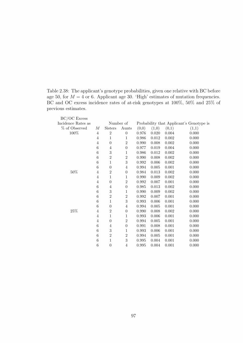
Table 2.38: The applicant’s genotype probabilities, given one relative with BC beforeage 50, for M = 4 or 6. Applicant age 30. ‘High’ estimates of mutation frequencies.BC and OC excess incidence rates of at-risk genotypes at 100%, 50% and 25% ofprevious estimates.
BC/OC ExcessIncidence Rates as Number of Probability that Applicant’s Genotype is
% of Observed M Sisters Aunts (0,0) (1,0) (0,1) (1,1)100% 4 2 0 0.976 0.020 0.004 0.000
4 1 1 0.986 0.012 0.002 0.0004 0 2 0.990 0.008 0.002 0.0006 4 0 0.977 0.019 0.004 0.0006 3 1 0.986 0.012 0.002 0.0006 2 2 0.990 0.008 0.002 0.0006 1 3 0.992 0.006 0.002 0.0006 0 4 0.994 0.005 0.001 0.000
50% 4 2 0 0.984 0.013 0.002 0.0004 1 1 0.990 0.009 0.002 0.0004 0 2 0.992 0.007 0.001 0.0006 4 0 0.985 0.013 0.002 0.0006 3 1 0.990 0.009 0.002 0.0006 2 2 0.992 0.007 0.001 0.0006 1 3 0.993 0.006 0.001 0.0006 0 4 0.994 0.005 0.001 0.000
25% 4 2 0 0.990 0.008 0.002 0.0004 1 1 0.993 0.006 0.001 0.0004 0 2 0.994 0.005 0.001 0.0006 4 0 0.991 0.008 0.001 0.0006 3 1 0.993 0.006 0.001 0.0006 2 2 0.994 0.005 0.001 0.0006 1 3 0.995 0.004 0.001 0.0006 0 4 0.995 0.004 0.001 0.000
97

Table 2.39: The applicant’s genotype probabilities, given two relatives with BCbefore age 50, for M = 4 or 6. Applicant age 30. ‘High’ estimates of mutationfrequencies. BC and OC excess incidence rates of at-risk genotypes at 100%, 50%and 25% of previous estimates.
BC/OC ExcessIncidence Rates as Number of Probability that Applicant’s Genotype is
% of Observed M Sisters Aunts (0,0) (1,0) (0,1) (1,1)100% 4 2 0 0.787 0.211 0.002 0.000
4 1 1 0.869 0.119 0.012 0.0004 0 2 0.910 0.081 0.009 0.0006 4 0 0.791 0.207 0.002 0.0006 3 1 0.869 0.121 0.010 0.0006 2 2 0.910 0.082 0.009 0.0006 1 3 0.933 0.061 0.007 0.0006 0 4 0.947 0.047 0.006 0.000
50% 4 2 0 0.897 0.101 0.002 0.0004 1 1 0.935 0.059 0.006 0.0004 0 2 0.952 0.043 0.005 0.0006 4 0 0.899 0.099 0.002 0.0006 3 1 0.935 0.060 0.005 0.0006 2 2 0.952 0.044 0.004 0.0006 1 3 0.962 0.034 0.004 0.0006 0 4 0.969 0.028 0.003 0.000
25% 4 2 0 0.959 0.039 0.002 0.0004 1 1 0.972 0.025 0.003 0.0004 0 2 0.978 0.020 0.002 0.0006 4 0 0.960 0.039 0.001 0.0006 3 1 0.972 0.026 0.003 0.0006 2 2 0.978 0.020 0.002 0.0006 1 3 0.981 0.017 0.002 0.0006 0 4 0.983 0.015 0.002 0.000
98
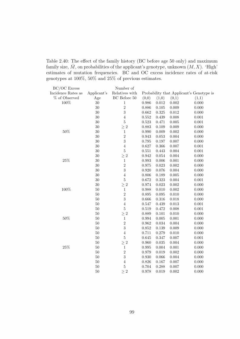
Table 2.40: The effect of the family history (BC before age 50 only) and maximumfamily size, M , on probabilities of the applicant’s genotype, unknown (M,X). ‘High’estimates of mutation frequencies. BC and OC excess incidence rates of at-riskgenotypes at 100%, 50% and 25% of previous estimates.
BC/OC Excess Number ofIncidence Rates as Applicant’s Relatives with Probability that Applicant’s Genotype is
% of Observed Age BC Before 50 (0,0) (1,0) (0,1) (1,1)100% 30 1 0.986 0.012 0.002 0.000
30 2 0.886 0.105 0.009 0.00030 3 0.662 0.325 0.012 0.00030 4 0.552 0.439 0.008 0.00130 5 0.523 0.471 0.005 0.00130 ≥ 2 0.883 0.109 0.009 0.000
50% 30 1 0.990 0.009 0.002 0.00030 2 0.943 0.053 0.004 0.00030 3 0.795 0.197 0.007 0.00030 4 0.627 0.366 0.007 0.00130 5 0.551 0.443 0.004 0.00130 ≥ 2 0.942 0.054 0.004 0.000
25% 30 1 0.993 0.006 0.001 0.00030 2 0.975 0.023 0.002 0.00030 3 0.920 0.076 0.004 0.00030 4 0.806 0.189 0.005 0.00030 5 0.672 0.323 0.004 0.00130 ≥ 2 0.974 0.023 0.002 0.000
100% 50 1 0.988 0.010 0.002 0.00050 2 0.895 0.095 0.010 0.00050 3 0.666 0.316 0.018 0.00050 4 0.547 0.439 0.013 0.00150 5 0.519 0.472 0.008 0.00150 ≥ 2 0.889 0.101 0.010 0.000
50% 50 1 0.994 0.005 0.001 0.00050 2 0.962 0.034 0.004 0.00050 3 0.852 0.139 0.009 0.00050 4 0.711 0.279 0.010 0.00050 5 0.645 0.347 0.007 0.00150 ≥ 2 0.960 0.035 0.004 0.000
25% 50 1 0.995 0.004 0.001 0.00050 2 0.979 0.019 0.002 0.00050 3 0.930 0.066 0.004 0.00050 4 0.826 0.167 0.007 0.00050 5 0.704 0.288 0.007 0.00050 ≥ 2 0.978 0.019 0.002 0.000
99

Chapter 3
Application of the breast and
ovarian cancer model to Critical
Illness insurance
In Section 2.5 we were concerned with the family history which develops before a
woman applies for insurance. Of particular importance was determining the prob-
abilities that a woman had BRCA1 or BRCA2 mutations given her family history.
Once the woman has been accepted for insurance, we are only concerned with events
in the insured’s life, and not in the relatives’ lives. We are interested in the oc-
currence of the events that will trigger claims according to the policy conditions.
Therefore there is a need to develop a model for the applicant to capture the onset of
claim triggering events. The models for pricing CI insurance discussed in Section 1.5
(Dash and Grimshaw (1990) and Dinani et al. (2000)) model the CI claims events
incidence with respect to the age and sex of the applicant. BCOC incidence is not
considered separately in these models but is grouped together with other cancers
and none of these models consider the family history of the applicant. Further the
model we need should explicitly incorporate the genotype of the applicant.
In this section we consider a woman applying for the stand-alone type of CI
policy defined in Section 1.5. We use a 28-day survival period. This should have
a negligible effect on the incidence of cancers but not so for other critical illnesses,
especially heart attacks and strokes.
100
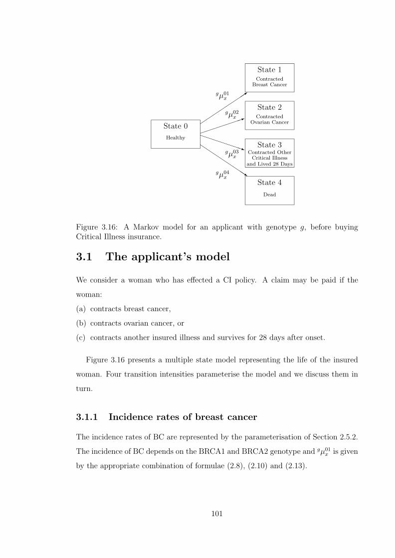
QQs
PPPPPPPq
³³³³³³³1´´
´´
´´
´3
State 0
Healthy
State 1Contracted
Breast Cancer
State 2Contracted
Ovarian Cancer
State 3Contracted Other
Critical Illnessand Lived 28 Days
State 4
Dead
gµ01x
gµ02x
gµ03x
gµ04x
Figure 3.16: A Markov model for an applicant with genotype g, before buyingCritical Illness insurance.
3.1 The applicant’s model
We consider a woman who has effected a CI policy. A claim may be paid if the
woman:
(a) contracts breast cancer,
(b) contracts ovarian cancer, or
(c) contracts another insured illness and survives for 28 days after onset.
Figure 3.16 presents a multiple state model representing the life of the insured
woman. Four transition intensities parameterise the model and we discuss them in
turn.
3.1.1 Incidence rates of breast cancer
The incidence rates of BC are represented by the parameterisation of Section 2.5.2.
The incidence of BC depends on the BRCA1 and BRCA2 genotype and gµ01x is given
by the appropriate combination of formulae (2.8), (2.10) and (2.13).
101

3.1.2 Incidence rates of ovarian cancer
The OC incidence, gµ02x , also differs by genotype and the transition intensities are
given by the appropriate combination of formulae (2.9), (2.12) and (2.14).
3.1.3 Incidence of other critical illness and surviving 28 days
The incidence rate of other critical illness will be the sum of the four components
listed below.
(a) The incidence rate of cancers which are not any of BC, OC or skin cancer which
is not malignant melanoma, since the latter does not trigger a CI claim.
(b) The incidence rate of heart attack with 28-day survival from onset.
(c) The incidence rate of stroke with 28-day survival from onset.
(d) The incidence rate of all other CI claim causes which are not covered by items
(a) to (c) and which are neither BC nor OC.
We discuss the modelling of these four components in turn.
Incidence of other cancers
‘Other Cancers’ are defined to exclude BC, OC and all skin cancer which is not
malignant melanoma. Skin cancer which is not malignant melanoma is specifically
excluded from the definition of cancer for critical illness policies. We assume that
the incidence of ‘Other Cancers’ is the same for all BRCA1 and BRCA2 genotypes
and this incidence is equal to that of the general population.
In a way similar to the parameterisation of the incidence of BC and OC in the
population in Section 2.5.2, we consider 1 January 1990 to 31 December 1992 as the
period of investigation. Using data from O.N.S. (1999), we calculate the number of
new cases of ‘Other Cancer’ for lives aged x, θx, for individual ages. The exposed to
risk, Ecx, is the same as was used in Section 2.5.2. Using these exposures means we
are not taking into account the women in the population who already have ‘Other
Cancers’. While we could safely ignore the lives with disease in the BC and OC
exposed to risk calculations in Section 2.5.2, the effect may not be negligible with
‘Other Cancers’. The effect of not subtracting the affected lives from the exposed to
102

risk would be that the estimated incidence rates will be lower than they should be.
However the numbers of new cases of ‘Other Cancers’ calculated from O.N.S. (1999)
include cancers, which though they may be the first ever of its type, may not be the
first ever cancer in the individual. CI claims would normally be triggered by the
first to occur of all cancers. We expect the inclusion of subsequent cancers to result
in estimated incidence rates which are higher than they should be. Our assumption
is that these effects of lowering and increasing the incidence rates should cancel each
other out. The exposed to risk values and the numbers of cases which we use are
shown in Appendix D. Based on the crude estimates of the incidence rates
µotherx =
θx
Ecx
.
Using unweighted least squares, we fitted the function
µotherx = exp(−10.3995 + 0.08235x) for x < 40 (3.26)
µotherx = 0.00808− 0.00019x
+0.000016(x− 35)2 − 0.000000144(x− 35)3 for x > 64 (3.27)
to represent the smooth incidence of ‘Other Cancers’. Between ages 40 and 64 we
used a linear blending of the two functions. The fitted function together with the
crude estimates are shown in Figure 3.17.
In cancer it is difficult to establish the exact day of onset of the disease. The
diagnosis process may take time and we consider it reasonable to assume that all
lives who develop any cancer will survive the 28 days necessary for them to claim
a CI benefit. This assumption is supported by estimated 28-day cancer survival
factors supplied to us by Swiss Re, which are equal to one at all ages.
Incidence of heart attacks
We assume that the incidence rates of heart attacks are the same irrespective of
BRCA1 or BRAC2 genotype and these are equal to the population incidence rates.
To estimate the incidence of heart attacks in the population we use data from the
Morbidity Statistics from General Practice (M.S.G.P.) Survey conducted between
September 1991 and August 1992. The survey was carried out in 60 practices in
England and Wales and accumulated about 250,000 person-years of exposure for
females. Based on this survey a CD-ROM was published which contains anonymised
103

Age
Inci
denc
e ra
te
0 20 40 60 80
0.0
0.00
50.
010
0.01
5
Figure 3.17: The observed and fitted incidence of ‘Other Cancers’ in the generalpopulation of England and Wales.
details of times spent in the study and General Practice consultations made during
the study year.
For CI purposes we define heart attack as the disease covered under International
Classification of Diseases (ICD) codes 410 and 414, and we only consider first-ever
cases. We are able to calculate, from the CD-ROM data, the exact exposed to risk,
Ecx for various age groups and the number of first-ever cases of heart attack, θx.
These are shown in Table 3.41.
Using unweighted least squares, the crude incidence rates, µheartx were graduated
by the Gamma function
µheartx = 0.58
(0.1616.34 exp(−0.16x)x15.34
Γ(16.34)
). (3.28)
Figure 3.18 shows the crude incidence rates and the graduated function. The CI
Healthcare Study Group published a CI base table with estimated incidence of heart
attacks in females (Dinani et al. (2000)). They consider a number of adjustments
to their crude rates and give, among other rates, ‘smoothed adjusted crude rates’.
104

Table 3.41: Exposed to risk, observed number of cases and crude incidence ratesof first-ever heart attack (ICD 410 and 414) amoung women. (Source: McCormicket al. (1995).)
Age Ecx θx µheart
x Age Ecx θx µheart
x
0–29 97,198.27 1 0.0000103 65–69 11,042.57 46 0.004165730–44 51,726.74 6 0.0001160 70–74 10,047.81 48 0.004777245–49 14,994.75 7 0.0004668 75–79 8,348.98 66 0.007905250–54 11,852.14 12 0.0010125 80–84 6,268.98 49 0.007816355–59 11,129.62 24 0.0021564 85–89 3,483.31 31 0.008899660–64 11,126.07 31 0.0027862 90–94 1,292.34 9 0.0069641
These are not adjusted for the 28-day survival requirement. In Figure 3.19 we show
their ‘smoothed adjusted crude rates’ together with the rates given by our graduation
of Equation (3.28). Figure 3.19 shows a very good agreement between the two sets
of rates especially at ages below 70 which are of main interest to us.
Of those lives who develop heart attack a significant proportion will not survive
for 28 days after disease onset. Only those who survive will be eligible for a CI
payout. In a community study in Glasgow, Morrison et al. (1997) found an overall
28-day survival of 50%. The survival proportion decreases with age. There is no
consensus, in the studies, on whether sex is an independent factor in the survival
rate. There are differences in population age distribution, many other characteristics
and type of treatment after admission to hospital following a heart attack, between
males and females. These differences may contribute to the apparent lower survival
rate in women (Morrison et al. (1997)). In general the probability of survival depends
mainly on two factors:
(a) chance of reaching the hospital alive after an attack, and
(b) type of treatment after admission to hospital.
Morrison et al. (1997) find socioeconomic differences affecting the chance of get-
ting to hospital alive after an attack. This is thought to be due to factors like
difficulty of recognising symptoms which may be more common in less educated
people. Morrison et al. (1997) did not find socioeconomic differences affecting the
survival once admitted to hospital.
105
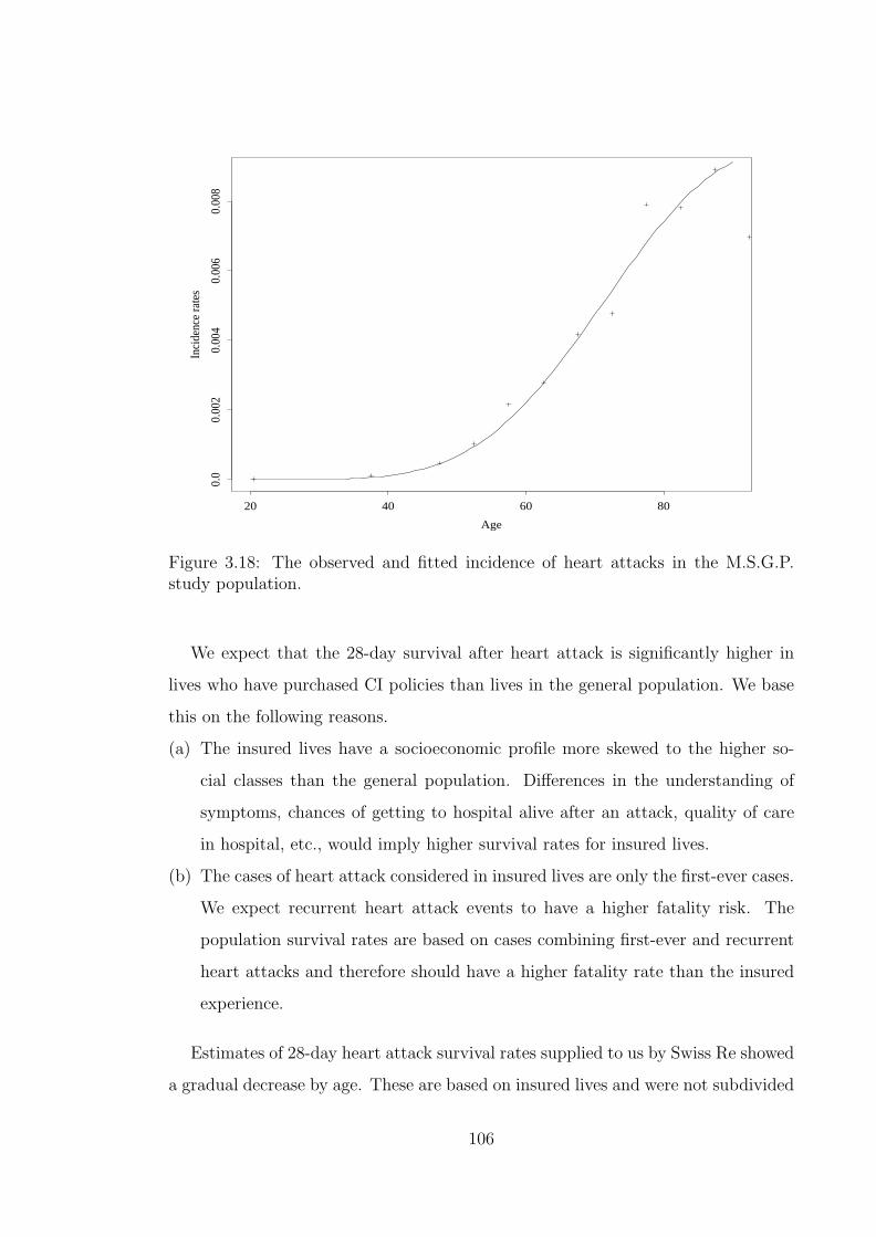
Age
Inci
denc
e ra
tes
20 40 60 80
0.0
0.00
20.
004
0.00
60.
008
Figure 3.18: The observed and fitted incidence of heart attacks in the M.S.G.P.study population.
We expect that the 28-day survival after heart attack is significantly higher in
lives who have purchased CI policies than lives in the general population. We base
this on the following reasons.
(a) The insured lives have a socioeconomic profile more skewed to the higher so-
cial classes than the general population. Differences in the understanding of
symptoms, chances of getting to hospital alive after an attack, quality of care
in hospital, etc., would imply higher survival rates for insured lives.
(b) The cases of heart attack considered in insured lives are only the first-ever cases.
We expect recurrent heart attack events to have a higher fatality risk. The
population survival rates are based on cases combining first-ever and recurrent
heart attacks and therefore should have a higher fatality rate than the insured
experience.
Estimates of 28-day heart attack survival rates supplied to us by Swiss Re showed
a gradual decrease by age. These are based on insured lives and were not subdivided
106

Age
Inci
denc
e ra
tes
20 30 40 50 60 70 80
0.0
0.00
20.
004
0.00
60.
008
Dinani et al.’s rates
Figure 3.19: Comparison of heart attack incidence rates in our graduation withthose by the CI Healthcare Study Group. (Source: Dinani et al. (2000).)
by sex. We graduated the survival factors using unweighted least squares by the
quadratic function
pheartx = 0.8983095− 0.00235911x− 0.00001359781x2. (3.29)
Figure 3.20 shows the population 28-day heart attack survival factors from the study
by Morrison et al. (1997) against the survival factors of insured lives as represented
by formula (3.29). It is not possible to determine neither the original source nor the
quality of the Swiss Re data. The large difference in the survival rates between the
Swiss Re values and those of Morrison et al. (1997) at the young ages is particularly
worrying. However in the absence of other insured lives data, we use the Swiss Re
rates.
From formulae (3.28) and (3.29), the incidence rate of heart attacks is therefore
reduced to
µheartx pheart
x . (3.30)
107
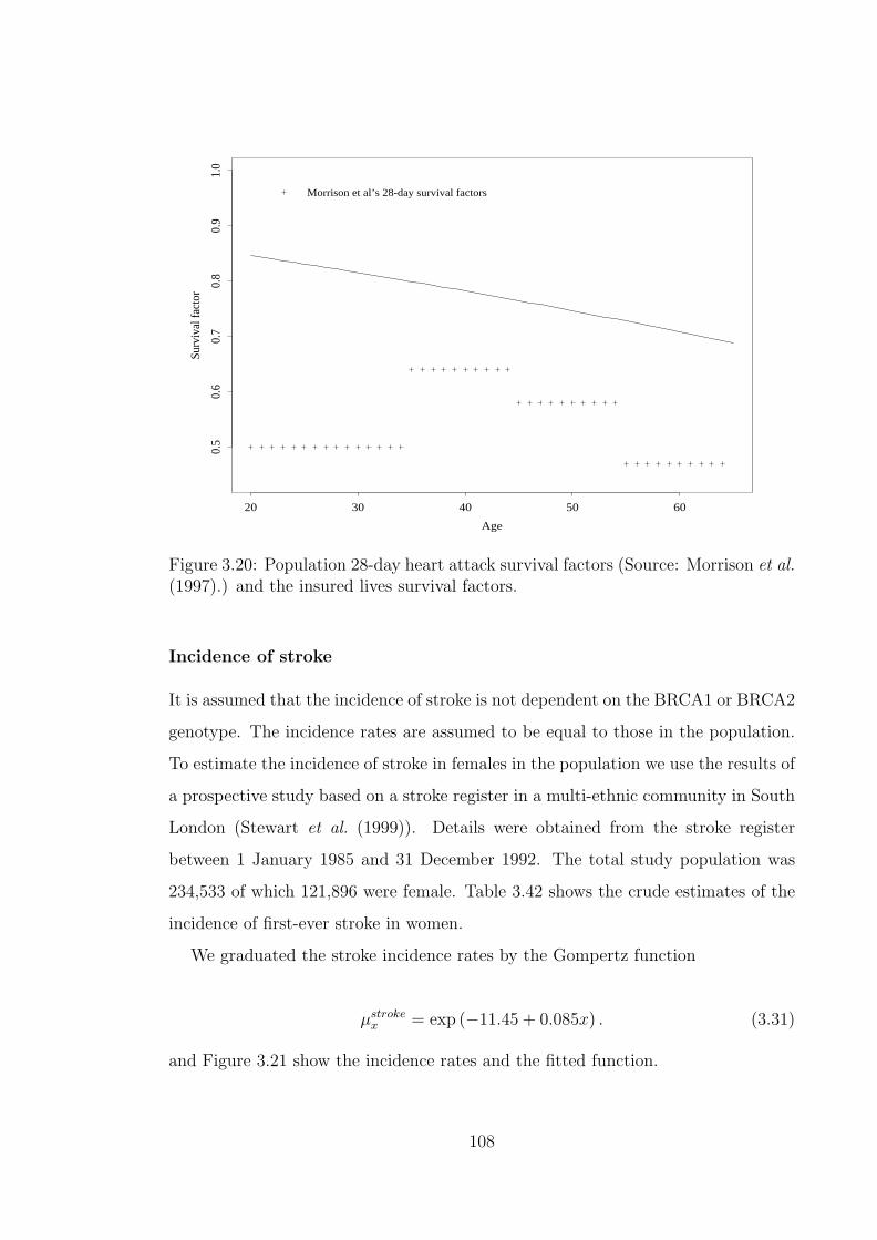
Age
Surv
ival
fact
or
20 30 40 50 60
0.5
0.6
0.7
0.8
0.9
1.0
Morrison et al’s 28-day survival factors
Figure 3.20: Population 28-day heart attack survival factors (Source: Morrison et al.(1997).) and the insured lives survival factors.
Incidence of stroke
It is assumed that the incidence of stroke is not dependent on the BRCA1 or BRCA2
genotype. The incidence rates are assumed to be equal to those in the population.
To estimate the incidence of stroke in females in the population we use the results of
a prospective study based on a stroke register in a multi-ethnic community in South
London (Stewart et al. (1999)). Details were obtained from the stroke register
between 1 January 1985 and 31 December 1992. The total study population was
234,533 of which 121,896 were female. Table 3.42 shows the crude estimates of the
incidence of first-ever stroke in women.
We graduated the stroke incidence rates by the Gompertz function
µstrokex = exp (−11.45 + 0.085x) . (3.31)
and Figure 3.21 show the incidence rates and the fitted function.
108

Table 3.42: Incidence rates of first-ever stroke among women. (Source: Stewartet al. (1999).)
Age Incidence Rate Age Incidence Rate< 15 0.00000 55–64 0.0013615–24 0.00005 65–74 0.0044525–34 0.00009 75–84 0.0089835–44 0.00034 ≥ 85 0.0188745–54 0.00078
Age
Inci
denc
e ra
tes
20 40 60 80
0.0
0.00
50.
010
0.01
50.
020
Figure 3.21: The observed and fitted incidence of stroke.
109

Table 3.43: Exposed to risk, cases and incidence rates of stroke from the M.S.G.P.study ( Source: McCormick et al. (1995)) and incidence rates of stroke from theO.C.S.P. ( Source: Bamford et al. (1988).)
M.S.G.P O.C.S.PAge Ec
x θx µstroke,M.S.G.Px µstroke,O.C.S.P
x
0–44 148,925.01 7 0.000047 0.00011045–54 26,846.89 19 0.000708 0.00046055–64 22,255.69 35 0.001573 0.00235065–74 21,090.38 82 0.003888 0.00584075–84 14,617.96 139 0.009509 0.01339085–90 3,866.28 66 0.017071 0.020360
There are two other possible source of stroke incidence rates which we considered.
One of them is the M.S.G.P. survey ( McCormick et al. (1995)) and the other is the
Oxfordshire Community Stroke Project (O.C.S.P.) study of 1981 to 1986 (Bamford
et al. (1988)). From the M.S.G.P. CD-ROM we can calculate the number of cases
of first-ever stroke recorded during the study, as we did for heart attacks. From
these cases and using the exposed to risk values we can estimate the incidence of
first-ever stroke. In Table 3.43 we show the exposed to risk, number of cases and
the incidence of first ever stroke based on the M.S.G.P. study. We also show the
incidence rates given by the O.C.S.P. study.
In Figure 3.22 we show the rates from the two studies together with our graduated
function given by Equation (3.31). It shows a good agreement for the three sets of
rates. It is expected that the rates from the M.S.G.P. study would be lower than
other since they do not capture all events outside the General Practice system. We
feel that the rates from Stewart et al. (1999) are the most reasonable to use since
they are the most recent of the three.
We then compare our graduated function given by Equation (3.31) with the
incidence of stroke from the Dinani et al. (2000). Unlike heart attacks, we used
their ‘crude rate’ and not the ‘smoothed adjusted crude rate’. This is because the
latter is adjusted for overlap with other CI claim causes which is not comparable to
the rates from Stewart et al. (1999). This comparison is shown in Figure 3.23. The
points represent the Dinani et al. (2000) rates while the solid line is the graduated
110

Age
Inci
denc
e ra
tes
20 40 60 80
0.0
0.00
50.
010
0.01
50.
020
M.S.G.P. incidence ratesO.C.S.P. incidence rates
Figure 3.22: Incidence rates from M.S.G.P. and O.C.S.P. with the graduated func-tion for stroke based on Stewart et al. (1999).
function. It shows remarkable agreement in the two sets of rates.
The 28-day stroke survival rates are somewhat higher than those of heart attack.
For reasons similar to those for heart attack survival factors, we expect the survival
factors for insured lives to be higher than those for the general population. Based on
the data supplied to us by Swiss Re we represent the 28-day stroke survival factors
in insured lives by the quadratic function
pstrokex = 0.8718412 + 0.001566578x− 0.00003711161x2. (3.32)
We compare the survival factors given by Equation (3.32) with population esti-
mates based on a study by Vemmos et al. (1999) carried out in southern Greece.
The incidence rate of stroke in the study population is similar to the stroke incidence
given by Stewart et al. (1999), shown in Table 3.42. The 28-day stroke survival fac-
tors from Vemmos et al. (1999) are shown in Figure 3.24. Vemmos et al. (1999) only
consider first-ever cases of stroke and therefore the population rates are closer to
the insured lives rates than we would expect if recurrent cases had been considered
111

Age
Inci
denc
e ra
tes
20 30 40 50 60 70 80
0.0
0.00
20.
004
0.00
60.
008
0.01
0Dinani et al’s rates
Figure 3.23: Comparison of stroke incidence rates in our graduation with those bythe CI Healthcare Study Group. (Source: Dinani et al. (2000).)
also.
Based on formulae (3.31) and (3.32), the incidence rates of stroke for the CI
model are reduced to
µstrokex pstroke
x . (3.33)
Incidence of ‘other CI claim causes’
CI claim causes which are not any of BC, OC, other cancers, heart attacks and stroke
still form a significant proportion of total CI claim causes. We classify these claim
causes as ‘minor’ causes and Table 3.44 shows the incidence rates of different causes
of CI claims for females, from a study of 1991–97 data by Dinani et al. (2000). We
note that ‘minor’ causes (causes not any of cancer, heart attack or stroke) account
for about 30% of claims below age 30 and about 15% of claims at other ages. We
make an allowance for the ‘minor’ claim causes by assuming that the incidence rate
of these causes is 15% of the sum of the incidence of cancer, heart attack and stroke
112

Age
Surv
ival
fact
or
20 40 60 80
0.6
0.7
0.8
0.9
1.0
Vemmos et al’s 28-day survival factors
Figure 3.24: Population 28-day stroke attack survival factors (Source: Vemmos et al.(1999).) and the insured lives survival factors.
for the same age. We note that cancer is composed of BC, OC and other cancers
of which BC and OC have incidence rates which differ by genotype. Irrespective
of the genotype we use the incidence of BC and OC for lives without mutations
for the purposes of calculating the incidence of ‘minor’ causes. This is equivalent to
assuming that incidence of ‘minor’ causes does not differ by genotype. The incidence
of ‘minor’ causes is therefore given by
0.15(µother
x + µstrokex pstroke
x + µheartx pheart
x + 0µ01x + 0µ02
x
). (3.34)
The total incidence of other critical illness, gµ03x , is then given by
gµ03x = 1.15
(µother
x + µstrokex pstroke
x + µheartx pheart
x
)+ 0.15
(0µ01
x + 0µ02x
)(3.35)
113

Table 3.44: Incidence rates (per 1,000) of CI claims by cause, for females in the U.K.in 1991–97. (Source: Dinani et al. (2000).)
Incidence Rate per 1,000 at AgeCause ≤ 30 31–40 41–50 51–60 ≥ 61Cancer 0.215 0.434 0.962 1.199 7.774Heart Attack 0.000 0.004 0.014 0.074 0.338Stroke 0.024 0.028 0.072 0.166 0.169Bypass Surgery 0.000 0.000 0.023 0.037 0.000Multiple Sclerosis 0.049 0.043 0.072 0.000 1.521Total Permanent Disability 0.034 0.021 0.099 0.184 0.000Other 0.015 0.015 0.014 0.018 0.169Total 0.337 0.545 1.255 1.678 9.971
3.1.4 Mortality
The mortality rate, gµ04x , represents the rate from deaths falling in two categories.
(a) Deaths due to causes which are not CI claim triggers. These are mostly acciden-
tal deaths at younger ages. At older ages these deaths are due to illnesses that
are not covered under CI insurance policies like respiratory disorders, digestive
system disorders and mental disorders. Injury from falls and being struck by
motor vehicles also contribute to accidental deaths in the elderly.
(b) Deaths due to causes which are CI claim triggers but the life dies within 28-days
of onset.
We represent component (a) by the mortality of ELT15F adjusted downwards
for a range of causes of death representing CI claim causes. We use Equation (2.16)
where θDx includes deaths due to cancer, heart attack, stroke, kidney failure, multiple
sclerosis, Alzheimer’s disease, Parkinson’s disease and benign brain tumour. From
O.N.S. (1999) we get the number of deaths due to cancer and from O.N.S. (1997a)
we get the total number of all deaths, θELT15Fx , both by single years of age. For the
remaining causes of death O.P.C.S. (1991b), O.P.C.S. (1993b) and O.P.C.S. (1993c)
give the number of deaths grouped in five year age groups. We aggregate the data
from O.N.S. (1999) and O.N.S. (1997a) into age groups corresponding to those of
O.P.C.S. (1991b), O.P.C.S. (1993b) and O.P.C.S. (1993c) and the values are shown
in Table 3.45.
The observed mortality adjustment factors
114

Table 3.45: Mortality data for adjusting ELT15F for CI causes of death.
Age range Total deaths CI deaths Age range Total deaths CI deathsx θELT15F
x θDx x θELT15F
x θDx
1–4 2.5 1,260 141 50–54 52 14,692 11,0505–9 7 682 197 55–59 57 23,377 17,693
10–14 12 651 128 60–64 62 41,022 30,82215–19 17 1,366 199 65–69 67 68,266 50,29820–24 22 1,875 378 70–74 72 93,083 67,06225–29 27 2,266 674 75–79 77 135,651 93,12030–34 32 2,887 1,315 80–84 82 169,605 109,48635–39 37 4,190 2,403 85–89 87 156,236 90,85340–44 42 7,105 4,781 90–94 92 91,033 45,52245–49 47 10,350 7,480
φfx =
θDx
θELT15Fx
(3.36)
were smoothed using the function
φfx =
−2.6129× 10⁻² + 1.0464× 10⁻¹ × x− 1.1814× 10⁻² × x2 + 4.6714× 10⁻⁴ × x3
−5.7901× 10⁻⁶ × x4 for x ≤ 30
−1.3451 + 8.9722× 10⁻² × x− 1.1998× 10⁻³ × x2 + 4.8678× 10⁻⁶ × x3
for x > 35.
(3.37)
Between the ages of 30 and 35, the two functions were linearly blended. The observed
mortality adjustment factors and the smoothed function are shown in Figure 3.25.
Recalling that we need to include the deaths within 28 days due to CI claim
causes, the mortality rate, gµ04x , is given by
gµ04x = µELT15F
x
(1− φf
x
)+
(µstroke
x − µstrokex pstroke
x
)+
(µheart
x − µheartx pheart
x
)= µELT15F
x
(1− φf
x
)+
(1− pstroke
x
)µstroke
x +(1− pheart
x
)µheart
x . (3.38)
115
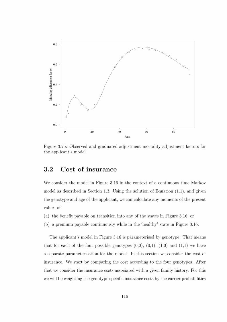
Age
Mor
talit
y ad
just
men
t fac
tor
0 20 40 60 80
0.0
0.2
0.4
0.6
0.8
Figure 3.25: Observed and graduated adjustment mortality adjustment factors forthe applicant’s model.
3.2 Cost of insurance
We consider the model in Figure 3.16 in the context of a continuous time Markov
model as described in Section 1.3. Using the solution of Equation (1.1), and given
the genotype and age of the applicant, we can calculate any moments of the present
values of
(a) the benefit payable on transition into any of the states in Figure 3.16; or
(b) a premium payable continuously while in the ‘healthy’ state in Figure 3.16.
The applicant’s model in Figure 3.16 is parameterised by genotype. That means
that for each of the four possible genotypes (0,0), (0,1), (1,0) and (1,1) we have
a separate parameterisation for the model. In this section we consider the cost of
insurance. We start by comparing the cost according to the four genotypes. After
that we consider the insurance costs associated with a given family history. For this
we will be weighting the genotype specific insurance costs by the carrier probabilities
116

associated with the family history.
In this section we consider only the first moments and we use the solution to
Equation (1.2). Thiele’s equations were solved using the Runge-Kutta procedure
(Conte and de Boor (1980)) with step size of 0.0005 years and force of interest
δ = 0.05.
3.2.1 Insurance costs by genotype
In Table 3.46 we present the expected present values (EPV) of CI cover of £1 for
various genotypes, various starting ages and various terms. The values shown can be
interpreted as the pure single premium required to secure the CI cover of £1 under a
stand alone CI insurance policy. In the first four rows we assume a population of the
uniform genotype given and in the last two rows we assume a population subdivided
into the four genotypes by proportions which depend on the mutation frequencies
used. (see Table 2.11). As expected from the fact that the (0,0) genotype dominates
the population genotype distribution, the EPV of the benefit under both the ‘high’
and the ‘low’ mutation assumptions are close to the EPV for the (0,0) genotype.
The three genotypes with mutations are associated with increased EPV for CI cover
compared to the population EPV’s.
Table 3.46: Expected present value (EPV) of Critical Illness cover of £1, depend-ing on BRCA1 and BRCA2 genotype, and based on ‘low’ and ‘high’ estimates ofmutation frequencies.
Age 30 at Entry Age 40 at Entry Age 50 at EntryTerm Term Term Term Term Term
Genotype 10 Yrs 20 Yrs 30 Yrs 10 Yrs 20 Yrs 10 Yrs(0,0) 0.010734 0.028080 0.049894 0.029113 0.065726 0.063195(1,0) 0.180706 0.350217 0.404920 0.369975 0.489364 0.370950(0,1) 0.022549 0.131668 0.261716 0.186436 0.408625 0.493542(1,1) 0.192506 0.401215 0.472231 0.465887 0.624401 0.643395Low 0.011013 0.028657 0.050589 0.029752 0.066609 0.063945High 0.010891 0.028404 0.050283 0.029472 0.066220 0.063614
Table 3.47 shows the EPV of an annuity of £1 per year paid continuously by
a life in the ‘healthy’ state in Figure 3.16. The values can be interpreted as the
117
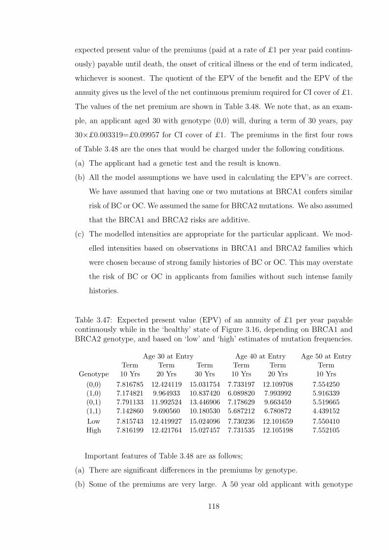
expected present value of the premiums (paid at a rate of £1 per year paid continu-
ously) payable until death, the onset of critical illness or the end of term indicated,
whichever is soonest. The quotient of the EPV of the benefit and the EPV of the
annuity gives us the level of the net continuous premium required for CI cover of £1.
The values of the net premium are shown in Table 3.48. We note that, as an exam-
ple, an applicant aged 30 with genotype (0,0) will, during a term of 30 years, pay
30×£0.003319=£0.09957 for CI cover of £1. The premiums in the first four rows
of Table 3.48 are the ones that would be charged under the following conditions.
(a) The applicant had a genetic test and the result is known.
(b) All the model assumptions we have used in calculating the EPV’s are correct.
We have assumed that having one or two mutations at BRCA1 confers similar
risk of BC or OC. We assumed the same for BRCA2 mutations. We also assumed
that the BRCA1 and BRCA2 risks are additive.
(c) The modelled intensities are appropriate for the particular applicant. We mod-
elled intensities based on observations in BRCA1 and BRCA2 families which
were chosen because of strong family histories of BC or OC. This may overstate
the risk of BC or OC in applicants from families without such intense family
histories.
Table 3.47: Expected present value (EPV) of an annuity of £1 per year payablecontinuously while in the ‘healthy’ state of Figure 3.16, depending on BRCA1 andBRCA2 genotype, and based on ‘low’ and ‘high’ estimates of mutation frequencies.
Age 30 at Entry Age 40 at Entry Age 50 at EntryTerm Term Term Term Term Term
Genotype 10 Yrs 20 Yrs 30 Yrs 10 Yrs 20 Yrs 10 Yrs(0,0) 7.816785 12.424119 15.031754 7.733197 12.109708 7.554250(1,0) 7.174821 9.964933 10.837420 6.089820 7.993992 5.916339(0,1) 7.791133 11.992524 13.446906 7.178629 9.663459 5.519665(1,1) 7.142860 9.690560 10.180530 5.687212 6.780872 4.439152Low 7.815743 12.419927 15.024096 7.730236 12.101659 7.550410High 7.816199 12.421764 15.027457 7.731535 12.105198 7.552105
Important features of Table 3.48 are as follows;
(a) There are significant differences in the premiums by genotype.
(b) Some of the premiums are very large. A 50 year old applicant with genotype
118
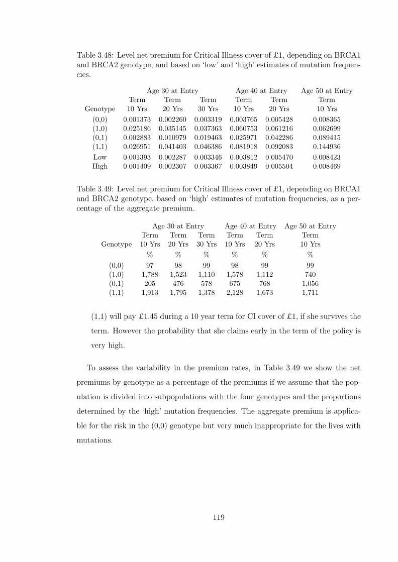
Table 3.48: Level net premium for Critical Illness cover of £1, depending on BRCA1and BRCA2 genotype, and based on ‘low’ and ‘high’ estimates of mutation frequen-cies.
Age 30 at Entry Age 40 at Entry Age 50 at EntryTerm Term Term Term Term Term
Genotype 10 Yrs 20 Yrs 30 Yrs 10 Yrs 20 Yrs 10 Yrs(0,0) 0.001373 0.002260 0.003319 0.003765 0.005428 0.008365(1,0) 0.025186 0.035145 0.037363 0.060753 0.061216 0.062699(0,1) 0.002883 0.010979 0.019463 0.025971 0.042286 0.089415(1,1) 0.026951 0.041403 0.046386 0.081918 0.092083 0.144936Low 0.001393 0.002287 0.003346 0.003812 0.005470 0.008423High 0.001409 0.002307 0.003367 0.003849 0.005504 0.008469
Table 3.49: Level net premium for Critical Illness cover of £1, depending on BRCA1and BRCA2 genotype, based on ‘high’ estimates of mutation frequencies, as a per-centage of the aggregate premium.
Age 30 at Entry Age 40 at Entry Age 50 at EntryTerm Term Term Term Term Term
Genotype 10 Yrs 20 Yrs 30 Yrs 10 Yrs 20 Yrs 10 Yrs% % % % % %
(0,0) 97 98 99 98 99 99(1,0) 1,788 1,523 1,110 1,578 1,112 740(0,1) 205 476 578 675 768 1,056(1,1) 1,913 1,795 1,378 2,128 1,673 1,711
(1,1) will pay £1.45 during a 10 year term for CI cover of £1, if she survives the
term. However the probability that she claims early in the term of the policy is
very high.
To assess the variability in the premium rates, in Table 3.49 we show the net
premiums by genotype as a percentage of the premiums if we assume that the pop-
ulation is divided into subpopulations with the four genotypes and the proportions
determined by the ‘high’ mutation frequencies. The aggregate premium is applica-
ble for the risk in the (0,0) genotype but very much inappropriate for the lives with
mutations.
119

3.2.2 Premium rating with complete knowledge of the fam-
ily history and structure
We now consider the premiums that would be payable assuming that we do not
know the genotype of the applicant but we know the family history and the family
size and structure. In the previous section we showed examples of the premiums as-
sociated with given genotypes. If we know the family history and the family size and
structure, we can calculate the genotype carrier probabilities as described in Section
2.5. Using the carrier probabilities we then calculate the premiums associated with
a family history as
the weighted average of the genotype specific EPV of unit benefit
the weighted average of the genotype specific EPV of unit annuity
where the weights are the genotype carrier probabilities. Using the notation of
Chapter 2, the above can be expressed as
E [E [PV of unit benefit|g1] |C(x)]
E [E [PV of unit annuity|g1] |C(x)].
We express the resulting premiums as a rating of the aggregate premium. The
aggregate premium is calculated as above but the weights are given genotype prob-
abilities of the ‘high’ mutation frequencies given in Table 2.11. We recall that the
rating represents the percentage of the aggregate premium to be added to the ag-
gregate premium such that a rating of +131 means that the rated premium is 231%
of the aggregate premium.
In Tables 3.50 to 3.55 we consider examples of a family history of BC. These are
considered in comparison with the underwriting guidelines of Table 2.3. The tables
show the following three aspects which are important in the underwriting.
(a) The age at entry is important to the underwriting. We note that Companies
B and C in Table 2.3 gave similar recommendations for applicants of different
ages.
(b) Knowledge of both the family size and structure is a very important factor in
the ratings. We note that family structure is not explicitly considered in the
ratings of Table 2.3.
120

Table 3.50: Level net premium for £1 CI benefit, given one relative with BC beforeage 50, for M = 4 or 6. ‘High’ estimates of mutation frequencies.
Premium as Rating of Aggregate PremiumNumber of Age 30 at Entry Age 50 at Entry
M Sisters Aunts 10 Yrs 20 Yrs 30 Yrs 10 Yrs4 2 0 +29 +22 +15 +64 1 1 +16 +12 + 8 +54 0 2 +11 + 8 + 6 +46 4 0 +28 +21 +14 +36 3 1 +16 +12 + 8 +26 2 2 +11 + 8 + 5 +26 1 3 + 7 + 6 + 4 +26 0 4 + 5 + 4 + 3 +2
(c) The term of the contract also has an effect on the ratings although at a smaller
level than age at entry and family structure. Term of contract is not explicitly
used in the ratings of Table 2.3.
Considering that roughly a rating of +200 or more will lead to declinature for
CI insurance, from Tables 3.50 and 3.51 an applicant with a family history of 1
affected relative with BC before age 50 will be accepted. The applicant would also
be accepted by all three companies in Table 2.3. However companies A and B will
recommend a rating of +100 or more in the premium while Tables 3.50 and 3.51
show that the ratings are very much below 100 and are likely to be considered as
standard premiums. Company C in Table 2.3 recommends a standard premium for
this family history. We note, however, that for applicants with family history of
1 BC before 50 family structure, term of contract, age at entry and use of ‘high’
mutation frequencies are not likely to give differences that would move the applicant
between rating classes.
We now consider an applicant with a family history of two relatives with BC
before age 50 and a known family size and structure. The premium ratings are
shown in Tables 3.52 and 3.53. We recall that Companies A and B in Table 2.3 would
decline such an applicant while Company C would give a rating of +50 regardless
of the age of the applicant. From Tables 3.52 and 3.53 we note the following:
(a) The ratings differ widely by family structure. Only the family structures for
which a sister has to be an affected relative are resulting in declinature.
121
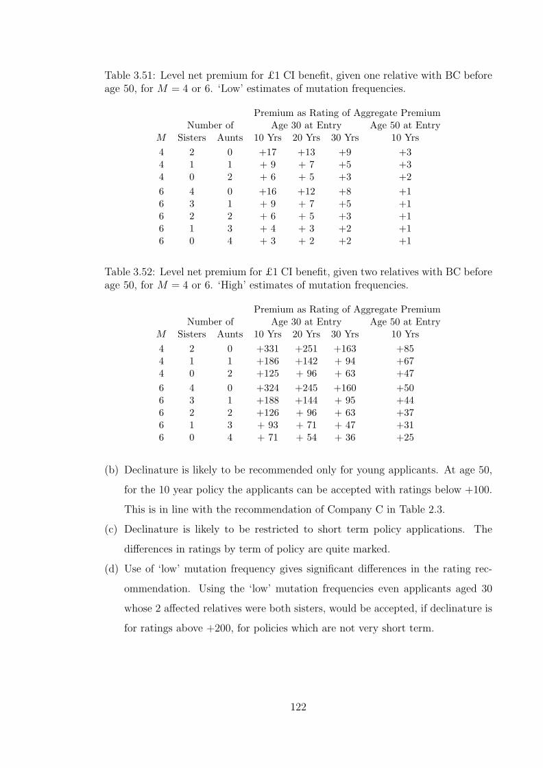
Table 3.51: Level net premium for £1 CI benefit, given one relative with BC beforeage 50, for M = 4 or 6. ‘Low’ estimates of mutation frequencies.
Premium as Rating of Aggregate PremiumNumber of Age 30 at Entry Age 50 at Entry
M Sisters Aunts 10 Yrs 20 Yrs 30 Yrs 10 Yrs4 2 0 +17 +13 +9 +34 1 1 + 9 + 7 +5 +34 0 2 + 6 + 5 +3 +26 4 0 +16 +12 +8 +16 3 1 + 9 + 7 +5 +16 2 2 + 6 + 5 +3 +16 1 3 + 4 + 3 +2 +16 0 4 + 3 + 2 +2 +1
Table 3.52: Level net premium for £1 CI benefit, given two relatives with BC beforeage 50, for M = 4 or 6. ‘High’ estimates of mutation frequencies.
Premium as Rating of Aggregate PremiumNumber of Age 30 at Entry Age 50 at Entry
M Sisters Aunts 10 Yrs 20 Yrs 30 Yrs 10 Yrs4 2 0 +331 +251 +163 +854 1 1 +186 +142 + 94 +674 0 2 +125 + 96 + 63 +476 4 0 +324 +245 +160 +506 3 1 +188 +144 + 95 +446 2 2 +126 + 96 + 63 +376 1 3 + 93 + 71 + 47 +316 0 4 + 71 + 54 + 36 +25
(b) Declinature is likely to be recommended only for young applicants. At age 50,
for the 10 year policy the applicants can be accepted with ratings below +100.
This is in line with the recommendation of Company C in Table 2.3.
(c) Declinature is likely to be restricted to short term policy applications. The
differences in ratings by term of policy are quite marked.
(d) Use of ‘low’ mutation frequency gives significant differences in the rating rec-
ommendation. Using the ‘low’ mutation frequencies even applicants aged 30
whose 2 affected relatives were both sisters, would be accepted, if declinature is
for ratings above +200, for policies which are not very short term.
122
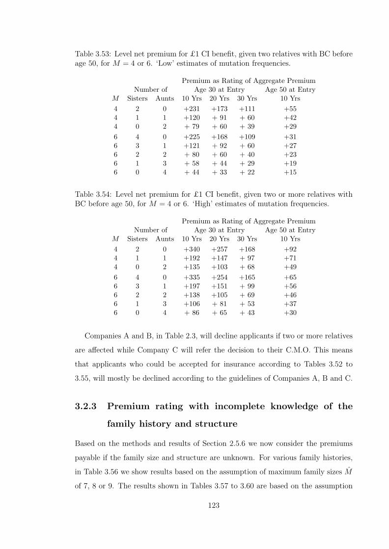
Table 3.53: Level net premium for £1 CI benefit, given two relatives with BC beforeage 50, for M = 4 or 6. ‘Low’ estimates of mutation frequencies.
Premium as Rating of Aggregate PremiumNumber of Age 30 at Entry Age 50 at Entry
M Sisters Aunts 10 Yrs 20 Yrs 30 Yrs 10 Yrs4 2 0 +231 +173 +111 +554 1 1 +120 + 91 + 60 +424 0 2 + 79 + 60 + 39 +296 4 0 +225 +168 +109 +316 3 1 +121 + 92 + 60 +276 2 2 + 80 + 60 + 40 +236 1 3 + 58 + 44 + 29 +196 0 4 + 44 + 33 + 22 +15
Table 3.54: Level net premium for £1 CI benefit, given two or more relatives withBC before age 50, for M = 4 or 6. ‘High’ estimates of mutation frequencies.
Premium as Rating of Aggregate PremiumNumber of Age 30 at Entry Age 50 at Entry
M Sisters Aunts 10 Yrs 20 Yrs 30 Yrs 10 Yrs4 2 0 +340 +257 +168 +924 1 1 +192 +147 + 97 +714 0 2 +135 +103 + 68 +496 4 0 +335 +254 +165 +656 3 1 +197 +151 + 99 +566 2 2 +138 +105 + 69 +466 1 3 +106 + 81 + 53 +376 0 4 + 86 + 65 + 43 +30
Companies A and B, in Table 2.3, will decline applicants if two or more relatives
are affected while Company C will refer the decision to their C.M.O. This means
that applicants who could be accepted for insurance according to Tables 3.52 to
3.55, will mostly be declined according to the guidelines of Companies A, B and C.
3.2.3 Premium rating with incomplete knowledge of the
family history and structure
Based on the methods and results of Section 2.5.6 we now consider the premiums
payable if the family size and structure are unknown. For various family histories,
in Table 3.56 we show results based on the assumption of maximum family sizes M
of 7, 8 or 9. The results shown in Tables 3.57 to 3.60 are based on the assumption
123

Table 3.55: Level net premium for £1 CI benefit, given two or more relatives withBC before age 50, for M = 4 or 6. ‘Low’ estimates of mutation frequencies.
Premium as Rating of Aggregate PremiumNumber of Age 30 at Entry Age 50 at Entry
M Sisters Aunts 10 Yrs 20 Yrs 30 Yrs 10 Yrs4 2 0 +237 +178 +115 +604 1 1 +124 + 94 + 62 +454 0 2 + 86 + 65 + 43 +316 4 0 +233 +175 +113 +416 3 1 +128 + 97 + 63 +346 2 2 + 88 + 67 + 44 +286 1 3 + 67 + 50 + 33 +236 0 4 + 53 + 40 + 26 +18
of a maximum family size of 9.
The ratings in Tables 3.56 and 3.57 show the following features.
(a) The number of relatives affected has a very strong influence on the ratings.
Ratings for a family history of 1 affected relative with BC before age 50 are very
much below +50. We note that Companies A and B in Table 2.3 recommended
ratings of +100 or higher for applicants with this family history for ages up to
50. Company C in the same table recommends standard premiums in this case.
Ratings for a family history of exactly 2 relatives with BC before 50 fall within
the insurable range. The ratings are similar to those recommended for a family
history of two or more relatives affected. As the exact number of relatives
affected rises above two the ratings rise steeply and are almost all above the
+200 rating above which declinature is normally recommended.
(b) For the 10 year policies shown, the difference in age at entry between 30 and
50 resulted in very significant differences in the ratings. As an example, the
applicants aged 50 with three relatives affected would be insurable.
(c) Longer terms for policies resulted in lower ratings. This difference is unlikely to
make a difference between insurability and declinature.
(d) Using ‘low’ mutation frequencies mostly resulted in reduced ratings. In some
cases there were slightly higher ratings for ‘low’ mutation frequencies than for
the ‘high’ frequencies. This is reasonable since the ratings are based on ag-
gregate premiums but the aggregate premium is dependent on the mutation
124
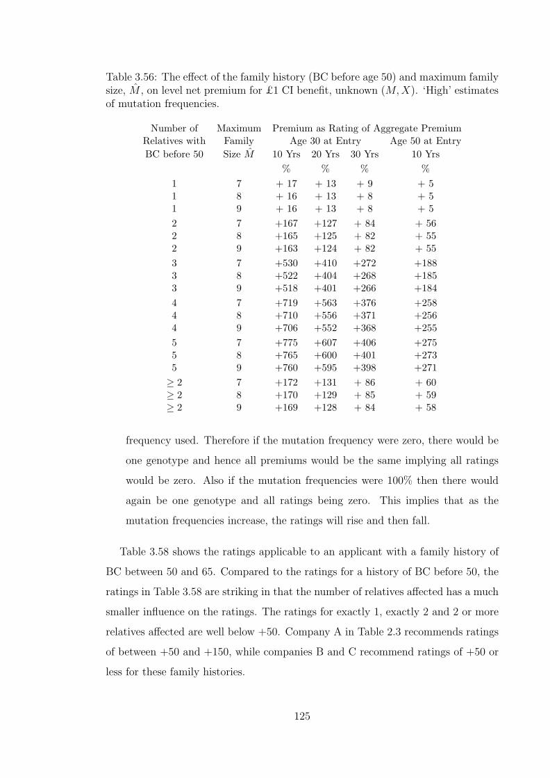
Table 3.56: The effect of the family history (BC before age 50) and maximum familysize, M , on level net premium for £1 CI benefit, unknown (M,X). ‘High’ estimatesof mutation frequencies.
Number of Maximum Premium as Rating of Aggregate PremiumRelatives with Family Age 30 at Entry Age 50 at EntryBC before 50 Size M 10 Yrs 20 Yrs 30 Yrs 10 Yrs
% % % %1 7 + 17 + 13 + 9 + 51 8 + 16 + 13 + 8 + 51 9 + 16 + 13 + 8 + 52 7 +167 +127 + 84 + 562 8 +165 +125 + 82 + 552 9 +163 +124 + 82 + 553 7 +530 +410 +272 +1883 8 +522 +404 +268 +1853 9 +518 +401 +266 +1844 7 +719 +563 +376 +2584 8 +710 +556 +371 +2564 9 +706 +552 +368 +2555 7 +775 +607 +406 +2755 8 +765 +600 +401 +2735 9 +760 +595 +398 +271≥ 2 7 +172 +131 + 86 + 60≥ 2 8 +170 +129 + 85 + 59≥ 2 9 +169 +128 + 84 + 58
frequency used. Therefore if the mutation frequency were zero, there would be
one genotype and hence all premiums would be the same implying all ratings
would be zero. Also if the mutation frequencies were 100% then there would
again be one genotype and all ratings being zero. This implies that as the
mutation frequencies increase, the ratings will rise and then fall.
Table 3.58 shows the ratings applicable to an applicant with a family history of
BC between 50 and 65. Compared to the ratings for a history of BC before 50, the
ratings in Table 3.58 are striking in that the number of relatives affected has a much
smaller influence on the ratings. The ratings for exactly 1, exactly 2 and 2 or more
relatives affected are well below +50. Company A in Table 2.3 recommends ratings
of between +50 and +150, while companies B and C recommend ratings of +50 or
less for these family histories.
125

Table 3.57: The effect of the family history (BC before age 50) on level net premiumfor £1 CI benefit, unknown (M,X). ‘Low’ estimates of mutation frequencies.
Number of Premium as Percentage of Aggregate PremiumRelatives with Age 30 at Entry Age 50 at EntryBC before 50 10 Yrs 20 Yrs 30 Yrs 10 Yrs
1 + 9 + 7 + 5 + 32 +107 + 81 + 53 + 353 +443 +340 +223 +1524 +693 +539 +358 +2475 +763 +596 +397 +270≥ 2 +110 + 83 + 54 + 37
Table 3.58: The effect of the family history (BC between ages 50–65) on level netpremium for £1 CI benefit, unknown (M,X).
Estimated Number of Premium as Rating of Aggregate PremiumMutation Relatives with Age 30 at Entry Age 50 at Entry
Frequencies BC between 50–65 10 Yrs 20 Yrs 30 Yrs 10 YrsHigh 1 + 2 + 3 + 2 + 2High 2 +11 + 15 + 14 + 12High 3 +29 + 52 + 54 + 53High 4 +48 +115 +131 +160High 5 +53 +154 +182 +277High ≥ 2 +11 + 15 + 14 + 13Low 1 + 1 + 1 + 1 + 1Low 2 + 7 + 8 + 8 + 7Low 3 +19 + 33 + 34 + 32Low 4 +39 + 92 + 103 +115Low 5 +50 +145 + 171 +244Low ≥ 2 + 7 + 9 + 8 + 7
A feature of the ratings in Table 3.58 which is not captured by the underwriting
recommendations in Table 2.3 is that applicants age 50 at entry have higher ratings
than applicants age 30. This is mainly due to the fact that for an applicant aged
30, a history of BC between ages 50 and 65 can only be observed in the mother
or aunt while for an applicant aged 50, this history can be observed in a sister.
The difference due to age at entry is very significant, and in some cases making the
difference between being insurable or not.
The premium ratings shown in Tables 3.59 and 3.60 are in respect of applicants
with family history of OC. Features listed below are generally similar to those for a
history of BC.
126

Table 3.59: The effect of the family history (OC before age 50) on level net premiumfor £1 CI benefit, unknown (M,X).
Estimated Number of Premium as Rating of Aggregate PremiumMutation Relatives with Age 30 at Entry Age 50 at Entry
Frequencies OC before 50 10 Yrs 20 Yrs 30 Yrs 10 YrsHigh 1 + 29 + 22 + 14 + 8High 2 +302 +229 +149 +104High 3 +664 +515 +341 +236High 4 +753 +588 +392 +266High 5 +780 +610 +407 +274High ≥ 2 +304 +230 +150 +105Low 1 + 17 + 13 + 8 + 5Low 2 +216 +162 +104 + 74Low 3 +630 +486 +320 +224Low 4 +756 +589 +391 +266Low 5 +785 +613 +407 +275Low ≥ 2 +217 +163 +105 + 75
(a) The number of relatives with OC has a very significant influence on the ratings.
This effect though seems to be modified by the age at onset of OC in the
relatives. In particular for 2 relatives affected with OC, the ratings are very
much lower if onset is between ages 50 and 65 than onset before 50.
(b) As the age at onset of OC in the relatives increases from below 50 to between
50 and 65, the ratings reduce.
(c) Longer term policies have ratings lower than shorter term policies.
3.2.4 The effect of lower BRCA1 and BRCA2 penetrance
In Section 2.5.7, we noted that there is generally a fall in estimated carrier proba-
bilities if the penetrance associated with mutations was reduced. We now consider
the influence of a reduction in penetrance on the premium ratings associated with
various family histories. In Table 3.61 we consider the premiums when the genotype
is known. Shown in the table are the level net premiums assuming that penetrance
is reduced by assuming excess BC and OC incidence rates of 50% and 25%. We
include the premiums based on the 100% excess risk (values previously given in
Table 3.49) for comparison. The aggregate premium used in the evaluation of Table
3.61 values is based on ‘high’ mutation frequency estimates. We note that there is a
127
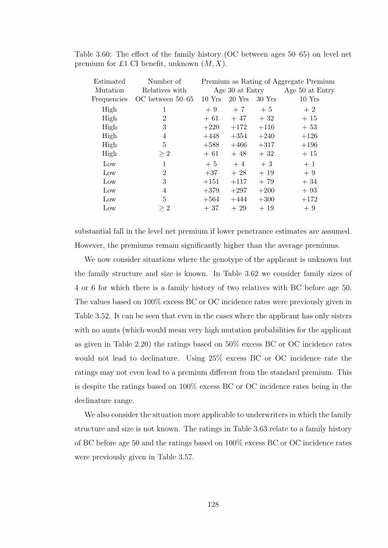
Table 3.60: The effect of the family history (OC between ages 50–65) on level netpremium for £1 CI benefit, unknown (M,X).
Estimated Number of Premium as Rating of Aggregate PremiumMutation Relatives with Age 30 at Entry Age 50 at Entry
Frequencies OC between 50–65 10 Yrs 20 Yrs 30 Yrs 10 YrsHigh 1 + 9 + 7 + 5 + 2High 2 + 61 + 47 + 32 + 15High 3 +220 +172 +116 + 53High 4 +448 +354 +240 +126High 5 +588 +466 +317 +196High ≥ 2 + 61 + 48 + 32 + 15Low 1 + 5 + 4 + 3 + 1Low 2 +37 + 28 + 19 + 9Low 3 +151 +117 + 79 + 34Low 4 +379 +297 +200 + 93Low 5 +564 +444 +300 +172Low ≥ 2 + 37 + 29 + 19 + 9
substantial fall in the level net premium if lower penetrance estimates are assumed.
However, the premiums remain significantly higher than the average premiums.
We now consider situations where the genotype of the applicant is unknown but
the family structure and size is known. In Table 3.62 we consider family sizes of
4 or 6 for which there is a family history of two relatives with BC before age 50.
The values based on 100% excess BC or OC incidence rates were previously given in
Table 3.52. It can be seen that even in the cases where the applicant has only sisters
with no aunts (which would mean very high mutation probabilities for the applicant
as given in Table 2.20) the ratings based on 50% excess BC or OC incidence rates
would not lead to declinature. Using 25% excess BC or OC incidence rate the
ratings may not even lead to a premium different from the standard premium. This
is despite the ratings based on 100% excess BC or OC incidence rates being in the
declinature range.
We also consider the situation more applicable to underwriters in which the family
structure and size is not known. The ratings in Table 3.63 relate to a family history
of BC before age 50 and the ratings based on 100% excess BC or OC incidence rates
were previously given in Table 3.57.
128

Table 3.61: Level net premium for Critical Illness cover of £1, depending on BRCA1and BRCA2 genotype, based on ‘high’ estimates of mutation frequencies , as apercentage of the aggregate premium. Excess BC and OC incidence rates 100%,50% or 25% of the levels observed among high-risk families.
ExcessBC/OC Risk Age 30 at Entry Age 40 at Entry Age 50 at Entry
as % of Term Term Term Term Term TermObserved Genotype 10 Yrs 20 Yrs 30 Yrs 10 Yrs 20 Yrs 10 Yrs
% % % % % %100% (0,0) 97 98 99 98 99 99100% (1,0) 1,788 1,523 1,110 1,578 1,112 740100% (0,1) 205 476 578 675 768 1,056100% (1,1) 1,913 1,795 1,378 2,128 1,673 1,71150% (0,0) 99 99 99 99 99 9950% (1,0) 968 857 642 852 608 41950% (0,1) 153 297 380 396 471 59550% (1,1) 1,035 1,033 856 1,151 954 92525% (0,0) 99 99 99 99 100 10025% (1,0) 540 491 381 479 355 25925% (0,1) 127 201 252 250 296 35225% (1,1) 575 592 518 635 566 518
3.3 Potential for adverse selection
We have, so far, made comparisons of costs of insurance between
(a) individual risk groups classified by genotype, detailed family history or sum-
marised family history, and
(b) the insured population considered as one group.
As expected, due to high BC and OC incidence rates associated with mutation
carriers and the rarity of mutations, the comparisons by genotype display very big
differences in the costs of insurance between genotypes. There are smaller, but
significant, differences in costs of insurance also between groups with different family
histories. However if we reconsider the results by genotype (see Table 3.49) we note
that even when using high mutation frequencies and high penetrance estimates in
the calculations, the low risk group (genotype (0, 0)) would pay 99% of the aggregate
premium. This means that by moving from being charged a premium determined
on the basis of the aggregate risk to being a charged a premium determined on the
risk of their subgroup alone, the low risk lives will not have a significant change in
129

Table 3.62: Level net premium for £1 CI benefit, given two relatives with BC beforeage 50, for M = 4 or 6. Applicant age 30. ‘High’ estimates of mutation frequencies.Excess BC and OC incidence rates 100%, 50% and 25% of the levels observed amonghigh-risk families.
BC/OC Excess Premium as Rating of Aggregate PremiumIncidence Rates as Number of Age 30 at Entry Age 50 at Entry
% of Observed M Sisters Aunts 10 Yrs 20 Yrs 30 Yrs 10 Yrs% % % %
100% 4 2 0 +331 + 251 + 163 + 854 1 1 +186 + 142 + 94 + 674 0 2 +125 + 96 + 63 + 476 4 0 +324 + 245 + 160 + 506 3 1 +188 + 144 + 95 + 446 2 2 +126 + 96 + 63 + 376 1 3 + 93 + 71 + 47 + 316 0 4 + 71 + 54 + 36 + 25
50% 4 2 0 + 83 + 68 + 46 + 174 1 1 + 49 + 40 + 28 + 134 0 2 + 35 +29 + 20 + 96 4 0 + 81 + 67 + 45 + 126 3 1 + 49 + 41 + 28 + 106 2 2 + 35 + 29 + 20 + 86 1 3 + 28 + 23 + 16 + 76 0 4 + 22 + 19 + 13 + 5
25% 4 2 0 + 16 + 14 + 10 + 54 1 1 + 10 + 9 + 6 + 44 0 2 + 8 + 7 + 5 + 26 4 0 + 16 + 14 + 10 + 46 3 1 + 10 + 9 + 6 + 36 2 2 + 8 + 7 + 5 + 36 1 3 + 7 + 6 + 4 + 26 0 4 + 6 + 5 + 4 + 2
130

Table 3.63: Level net premium for £1 CI benefit, given a history of BC before age50, unknown (M,X). Applicant age 30. ‘Low’ estimates of mutation frequencies.Excess BC and OC incidence rates 100%, 50% and 25% of the levels observed amonghigh-risk families.
BC/OC Excess Premium as Rating of Aggregate PremiumIncidence Rates as Relatives with Age 30 at Entry Age 50 at Entry
% of Observed BC Before 50 10 Yrs 20 Yrs 30 Yrs 10 Yrs% % % %
100% 1 + 9 + 7 + 5 + 32 + 107 +81 + 53 + 353 +443 +340 + 223 + 1524 +693 + 539 +358 + 2475 +763 + 596 +397 +270≥ 2 +110 + 83 + 54 + 37
50% 1 + 3 +3 + 2 + 12 +26 +21 + 15 + 63 + 118 +98 + 67 + 304 + 273 + 227 +156 + 745 +366 +306 + 211 + 101≥ 2 + 26 + 22 + 15 + 7
25% 1 + 1 + 1 + 1 + 02 + 5 + 5 + 3 + 23 + 20 + 17 + 12 + 64 + 57 + 49 +35 + 185 + 115 + 100 +70 + 37≥ 2 + 5 + 5 + 3 + 2
131
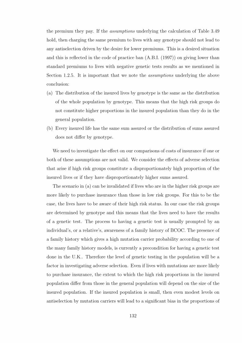
the premium they pay. If the assumptions underlying the calculation of Table 3.49
hold, then charging the same premium to lives with any genotype should not lead to
any antiselection driven by the desire for lower premiums. This is a desired situation
and this is reflected in the code of practice ban (A.B.I. (1997)) on giving lower than
standard premiums to lives with negative genetic tests results as we mentioned in
Section 1.2.5. It is important that we note the assumptions underlying the above
conclusion:
(a) The distribution of the insured lives by genotype is the same as the distribution
of the whole population by genotype. This means that the high risk groups do
not constitute higher proportions in the insured population than they do in the
general population.
(b) Every insured life has the same sum assured or the distribution of sums assured
does not differ by genotype.
We need to investigate the effect on our comparisons of costs of insurance if one or
both of these assumptions are not valid. We consider the effects of adverse selection
that arise if high risk groups constitute a disproportionately high proportion of the
insured lives or if they have disproportionately higher sums assured.
The scenario in (a) can be invalidated if lives who are in the higher risk groups are
more likely to purchase insurance than those in low risk groups. For this to be the
case, the lives have to be aware of their high risk status. In our case the risk groups
are determined by genotype and this means that the lives need to have the results
of a genetic test. The process to having a genetic test is usually prompted by an
individual’s, or a relative’s, awareness of a family history of BCOC. The presence of
a family history which gives a high mutation carrier probability according to one of
the many family history models, is currently a precondition for having a genetic test
done in the U.K.. Therefore the level of genetic testing in the population will be a
factor in investigating adverse selection. Even if lives with mutations are more likely
to purchase insurance, the extent to which the high risk proportions in the insured
population differ from those in the general population will depend on the size of the
insured population. If the insured population is small, then even modest levels on
antiselection by mutation carriers will lead to a significant bias in the proportions of
132
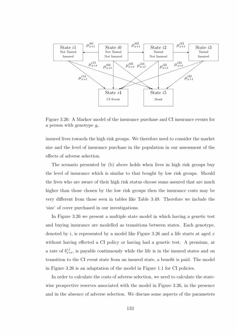
- -¾
? ?
ZZ
ZZ
ZZ
ZZ
ZZ~
ZZ
ZZ
ZZ
ZZ
ZZ~
½½
½½
½½
½½
½½=
½½
½½
½½
½½
½½=
PPPPPPPPPPPPPPPPPPPPPPq
³³³³³³³³³³³³³³³³³³³³³³)
State i0State i1 State i2 State i3
State i4
Not Tested
Not Insured
Not Tested
Insured
Tested
Not Insured
Tested
Insured
Dead
State i5
CI Event
µi01x+t µi02
x+t
µi05x+t
µi23x+t
µi34x+tµi25
x+t
µi14x+t
µi24x+tµi04
x+tµi15
x+t
µi35x+t
Figure 3.26: A Markov model of the insurance purchase and CI insurance events fora person with genotype gi.
insured lives towards the high risk groups. We therefore need to consider the market
size and the level of insurance purchase in the population in our assessment of the
effects of adverse selection.
The scenario presented by (b) above holds when lives in high risk groups buy
the level of insurance which is similar to that bought by low risk groups. Should
the lives who are aware of their high risk status choose sums assured that are much
higher than those chosen by the low risk groups then the insurance costs may be
very different from those seen in tables like Table 3.49. Therefore we include the
‘size’ of cover purchased in our investigations.
In Figure 3.26 we present a multiple state model in which having a genetic test
and buying insurance are modelled as transitions between states. Each genotype,
denoted by i, is represented by a model like Figure 3.26 and a life starts at aged x
without having effected a CI policy or having had a genetic test. A premium, at
a rate of bi,jx+t, is payable continuously while the life is in the insured states and on
transition to the CI event state from an insured state, a benefit is paid. The model
in Figure 3.26 is an adaptation of the model in Figure 1.1 for CI policies.
In order to calculate the costs of adverse selection, we need to calculate the state-
wise prospective reserves associated with the model in Figure 3.26, in the presence
and in the absence of adverse selection. We discuss some aspects of the parameters
133

of the models for this purpose.
Adverse selection
We model adverse selection by assuming that
(a) mutation carriers are more likely to have a genetic test,
(b) those who test positive may be more likely to buy insurance, or
(c) those who test positive may tend to buy larger amounts of insurance.
We can choose transition intensities and benefits in the model to reflect this
and assume that the insurance company charges everyone a premium based on the
incidence of CI claims in the whole population.
It should be noted that since insurance buying is a modelled event, the prospective
reserves are reserves in relation to the starting state in Figure 3.26 rather than the
insured states. The insurance buying model then affects the reserves such that the
lives that are more likely to buy insurance will need higher reserves at the outset.
Premiums
The statewise prospective reserves to be calculated satisfy Thiele’s Equations (1.2)
and are based on a Markov model. Therefore the premiums bi,jx+t can not depend
on the age at entry, since this is equivalent to having the reserves for some state
depending on the duration for which the life has occupied the state. We define the
premium to be proportional to the population average of the intensity of a CI event
at age x + t. It is therefore dependent on the current age and not age at entry. The
average uses weightings, by genotype, of the intensities of a CI event, of lives that
are in any of the healthy states. We assume that at age 30 the genotype distribution
in the population is exactly as given in Table 2.11. At subsequent ages the weights
are determined by the occupancy probabilities in the model of Figure 3.26 which
are obtained by solving the Kolmogorov forward equations (see Section 1.4.1).
Levels of genetic testing and insurance purchase
We assume two scenarios for the level of genetic testing. A ‘force of testing’, µi02x+t =
1.0 represents ‘high’ levels of genetic testing while µi02x+t = 0.1 represents ‘low’ levels
134
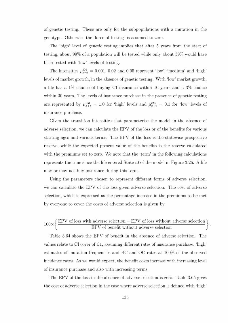
of genetic testing. These are only for the subpopulations with a mutation in the
genotype. Otherwise the ‘force of testing’ is assumed to zero.
The ‘high’ level of genetic testing implies that after 5 years from the start of
testing, about 99% of a population will be tested while only about 39% would have
been tested with ‘low’ levels of testing.
The intensities µi01x+t = 0.001, 0.02 and 0.05 represent ‘low’, ‘medium’ and ‘high’
levels of market growth, in the absence of genetic testing. With ‘low’ market growth,
a life has a 1% chance of buying CI insurance within 10 years and a 3% chance
within 30 years. The levels of insurance purchase in the presence of genetic testing
are represented by µi23x+t = 1.0 for ‘high’ levels and µi23
x+t = 0.1 for ‘low’ levels of
insurance purchase.
Given the transition intensities that parameterise the model in the absence of
adverse selection, we can calculate the EPV of the loss or of the benefits for various
starting ages and various terms. The EPV of the loss is the statewise prospective
reserve, while the expected present value of the benefits is the reserve calculated
with the premiums set to zero. We note that the ‘term’ in the following calculations
represents the time since the life entered State i0 of the model in Figure 3.26. A life
may or may not buy insurance during this term.
Using the parameters chosen to represent different forms of adverse selection,
we can calculate the EPV of the loss given adverse selection. The cost of adverse
selection, which is expressed as the percentage increase in the premiums to be met
by everyone to cover the costs of adverse selection is given by
100×{
EPV of loss with adverse selection− EPV of loss without adverse selection
EPV of benefit without adverse selection
}.
Table 3.64 shows the EPV of benefit in the absence of adverse selection. The
values relate to CI cover of £1, assuming different rates of insurance purchase, ‘high’
estimates of mutation frequencies and BC and OC rates at 100% of the observed
incidence rates. As we would expect, the benefit costs increase with increasing level
of insurance purchase and also with increasing terms.
The EPV of the loss in the absence of adverse selection is zero. Table 3.65 gives
the cost of adverse selection in the case where adverse selection is defined with ‘high’
135

Table 3.64: Expected present value (EPV) of benefit under a CI insurance of £1,for a woman untested and uninsured at outset, with no adverse selection. ‘High’estimates of mutation frequencies, and excess BC and OC incidence rates 100% ofthose observed. µi01
x+t represents the normal rate at which CI insurance is purchased.
Age 30 at Entry Age 40 at Entry Age 50 at EntryTerm Term Term Term Term Term
µi01x+t 10 Yrs 20 Yrs 30 Yrs 10 Yrs 20 Yrs 10 Yrs
0.001 0.000060 0.000328 0.000870 0.000157 0.000706 0.0003180.01 0.000583 0.003082 0.007930 0.001521 0.006644 0.0030910.05 0.002554 0.011907 0.027497 0.006672 0.025941 0.013609
levels of genetic testing and ‘high’ levels of insurance purchase but does not include
purchase of more than average sums assured by the adverse selectors. The rate of
normal insurance purchase (or market size) has a very big influence on the costs of
adverse selection. In a large market (µi01x+t = 0.05), the costs are less than 10% of
the premiums. The corresponding costs are lower when assuming lower mutation
frequencies (values not shown). Table 3.66 gives the corresponding costs of adverse
selection with ‘low’ levels of genetic testing and ‘low’ levels of insurance purchase by
lives with mutations. These values are also based on adverse selectors not choosing
sums assured which are higher than the average. For the medium or large markets,
the costs of adverse selection are below 5% of the premiums.
In Tables 3.67 and 3.68 we show the costs of adverse selection in cases where
the adverse selectors choose higher than average sum assured values. In both tables
we consider penetrance of 25% of the observed excess BC and OC rates and ‘high’
mutation frequencies. In Table 3.67 we assume ‘high’ levels of genetic testing and
insurance purchase while in Table 3.68 we use the ‘low’ levels. They show that the
costs of adverse selection are significant if the selectors are allowed to purchase much
higher sums assured than the average. These costs can be extreme if the market is
small or emerging.
We conclude that the effect of adverse selection on CI policies, with respect to
BRCA1 and BRCA2 mutations is only likely to be significant if:
(a) The CI insurance market is very small. In the UK, annual sales of stand-alone
CI policies reached about 700,000 in 1998 and the total number of policies in
force was about 2,400,000 (see Dinani et al. (2000)). Considering that there are
136
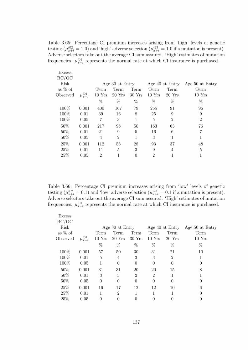
Table 3.65: Percentage CI premium increases arising from ‘high’ levels of genetictesting (µi02
x+t = 1.0) and ‘high’ adverse selection (µi23x+t = 1.0 if a mutation is present).
Adverse selectors take out the average CI sum assured. ‘High’ estimates of mutationfrequencies. µi01
x+t represents the normal rate at which CI insurance is purchased.
ExcessBC/OC
Risk Age 30 at Entry Age 40 at Entry Age 50 at Entryas % of Term Term Term Term Term Term
Observed µi01x+t 10 Yrs 20 Yrs 30 Yrs 10 Yrs 20 Yrs 10 Yrs
% % % % % %100% 0.001 400 167 79 255 91 96100% 0.01 39 16 8 25 9 9100% 0.05 7 3 1 5 2 250% 0.001 217 98 50 163 63 7650% 0.01 21 9 5 16 6 750% 0.05 4 2 1 3 1 125% 0.001 112 53 28 93 37 4825% 0.01 11 5 3 9 4 525% 0.05 2 1 0 2 1 1
Table 3.66: Percentage CI premium increases arising from ‘low’ levels of genetictesting (µi02
x+t = 0.1) and ‘low’ adverse selection (µi23x+t = 0.1 if a mutation is present).
Adverse selectors take out the average CI sum assured. ‘High’ estimates of mutationfrequencies. µi01
x+t represents the normal rate at which CI insurance is purchased.
ExcessBC/OC
Risk Age 30 at Entry Age 40 at Entry Age 50 at Entryas % of Term Term Term Term Term Term
Observed µi01x+t 10 Yrs 20 Yrs 30 Yrs 10 Yrs 20 Yrs 10 Yrs
% % % % % %100% 0.001 57 50 30 31 21 10100% 0.01 5 4 3 3 2 1100% 0.05 1 0 0 0 0 050% 0.001 31 31 20 20 15 850% 0.01 3 3 2 2 1 150% 0.05 0 0 0 0 0 025% 0.001 16 17 12 12 10 625% 0.01 1 2 1 1 1 025% 0.05 0 0 0 0 0 0
137

Table 3.67: Percentage CI premium increases arising from ‘high’ levels of genetictesting (µi02
x+t = 1.0) and ‘high’ adverse selection (µi23x+t = 1.0 if a mutation is present).
Adverse selectors take out one, two or four times the average CI sum assured. ‘High’mutation frequencies and excess BC and OC incidence 25% of that observed. µi01
x+t
represents the normal rate at which CI insurance is purchased.
Sum Assured Age 30 at Entry Age 40 at Entry Age 50 at Entryof ‘Adverse Term Term Term Term Term TermSelectors’ µi01
x+t 10 Yrs 20 Yrs 30 Yrs 10 Yrs 20 Yrs 10 Yrs% % % % % %
1 × average 0.001 112 54 28 85 34 401 × average 0.01 11 5 3 8 3 41 × average 0.05 2 1 0 2 1 12 × average 0.001 225 108 57 169 68 812 × average 0.01 22 11 6 17 7 82 × average 0.05 5 2 1 3 2 24 × average 0.001 450 216 114 339 136 1614 × average 0.01 46 22 12 34 14 164 × average 0.05 10 5 3 7 3 3
Table 3.68: Percentage CI premium increases arising from ‘low’ levels of genetictesting (µi02
x+t = 0.1) and ‘low’ adverse selection (µi23x+t = 0.1 if a mutation is present).
Adverse selectors take out two or four times the average CI sum assured. Highmutation frequencies and excess BC and OC incidence 25% of that observed. µi01
x+t
represents the normal rate at which CI insurance is purchased.
Sum Assured Age 30 at Entry Age 40 at Entry Age 50 at Entryof ‘Adverse Term Term Term Term Term TermSelectors’ µi01
x+t 10 Yrs 20 Yrs 30 Yrs 10 Yrs 20 Yrs 10 Yrs% % % % % %
1 × average 0.001 16 17 12 11 8 51 × average 0.01 1 2 1 1 1 01 × average 0.05 0 0 0 0 0 02 × average 0.001 32 35 24 23 19 112 × average 0.01 3 3 2 2 2 12 × average 0.05 0 1 0 0 0 04 × average 0.001 64 70 49 47 39 234 × average 0.01 6 7 5 5 4 24 × average 0.05 1 1 1 1 1 0
138
lives covered by group policies (about 50,000 in 1998) and others covered by
accelerated benefit policies, we feel that the UK CI market is larger than would
be significantly affected by adverse selection. This may not be true for other
markets like the U.S.A.
(b) High sums assured can be obtained without disclosing known genetic test results
or family history.
(c) The high penetrances observed for mutation carriers which are based on mem-
bers of high risk families are applicable to mutation carriers from other families.
3.4 Discussion
The detailed information available on the genetics of breast and ovarian cancer has
enabled us to produce the insurance costs by genotype and to produce a family
history model. Using the family history model, we could produce insurance costs by
detailed family history or by summarised family history. As a result we managed
to quantify the potential costs of adverse selection should genetic information be
unavailable to the underwriters. The important aspects and parameters of our
model include:
(a) penetrance estimates,
(b) mutation frequencies, and
(c) behaviour of adverse selectors.
If the assumptions that we make on these aspects and parameters closely reflect
the reality of the U.K. market (which will become clearer as genetics advances and
more data becomes available), then a position on BCOC like that of the current
moratorium on genetic test results except for CI policies with sum assured above
£300,000 should be sustainable. It is imperative that the experience in the UK
population, with respect to the important parameters in our model, is monitored as
time progresses.
There is need for further work to extend our model to other types of life and health
insurance. The most obvious is to consider life insurance. This is appropriate in
that a large proportion of CI policies are sold as riders to life insurance policies. To
139

achieve this we need to estimate the transition intensities representing the mortality
of women with breast or ovarian cancer. The force of mortality after onset of BC or
OC depends on, amoung others, the following factors.
(a) Any factors that affect prognosis after treatment. These include aspects associ-
ated with cancer staging at diagnosis like tumour size, extent of tumour spread
(Souhami and Tobias (1998)), etc.
(b) Age.
(c) Time elapsed since diagnosis.
Our modelling does not capture the details of the cancer at diagnosis of the nature
described by (a) above although these are important indicators of the survival of the
patient. Some information about these indicators may be modelled by allowing for
differing expressivity of different genotypes. However if there are benefit payments
associated with onset of disease (as is the case in CI insurance), then the age at
diagnosis and, as a result, the duration since diagnosis is observable. We need to
model the mortality in women with BC or OC as a function of age and/or duration
since diagnosis.
This can be done using UK population data. Details of registered tumours in
England and Wales pertaining to age at diagnosis and survival time are given by
Coleman et al. (1999). The exact age at diagnosis is given and also the exact time
to death after diagnosis. Associated details like sex, tumour site, date of diagnosis,
are also given among others. These data are ideal for estimating age and duration
dependent mortality of BC and OC sufferers.
A particularly challenging aspect of this modelling of mortality is representing
the effect of the fast changing treatment methods which have resulted in significant
reductions in mortality especially at short and medium term durations.
With a life insurance model it will be possible to consider the costs of insurance
by genotype and assess the costs of adverse selection. Such results may be compared
with those from Lemaire et al. (2000) and Subramanian et al. (1999).
Lemaire et al. (2000) discussed the pricing of term assurance in the presence of
a family history of BCOC based on the model in Figure 2.3. The mortality of lives
with BC was assumed to be independent of both age and duration since onset of BC.
140

The mortality of OC patients was obtained by a projection of survival probabilities
(in the S.E.E.R. population (U.S.A)) to those expected for onset year 1992. The
survival for n years, independent of age and duration is represented by
S(n) = 1− 0.63 (1− exp(−0.333n)) .
They conclude that many women with a family history of BCOC can be insured
for term assurance at standard rates. However ratings are likely to be necessary for
applicants whose first degree relatives had cancer at an early age, or those with two
or more family members affected. We note that they compare the net premiums
associated with various family histories to those payable by a life with no family
history. In our results for CI, the premiums were compared to the premiums deter-
mined from the costs by genotype. Lemaire et al. (2000) also conclude that insurers
should ask for, and use, more information like the ages at onset of the affected
relatives in underwriting and pricing.
Subramanian et al. (1999) considers the costs of adverse selection if the adverse
selection can be triggered by a genetic test result but the insurance company can
price using family history only. Adverse selection can take the form of an increase
(in the case of an adverse genetic test result) or a decrease in the sum assured or the
decision to purchase or not to purchase insurance when they would not otherwise
do so. Under various assumptions of the rates of insurance purchase, lapse and re-
entry and a 5% level of genetic testing, they conclude that purchasing very high sum
assureds can lead to high costs of adverse selection. This is in agreement with our
conclusion for CI. They conclude that adverse selection is a problem that insurers
can control if they are allowed to use family history and the insurers apply strict
underwriting to ensure the full and correct family history is used.
Our results may overstate the costs of adverse selection due to our use of high rates
of genetic testing and high rates of adverse selection. However, they are based on the
analysis of two rare genetic disorders and we have not taken into consideration that
BRCA1 and BRCA2 gene mutations may lead to increased risk of other cancers.
Ford et al. (1994) reported a significantly increased risk of colon cancer and of
prostate cancer in BRCA1 mutation carriers. To assess the impact of genetics on CI
141
insurance more fully we need to consider gene mutations that may be associated with
the other major critical illnesses, ‘other’ cancers and the cardiovascular disorders.
There are gene mutations associated with ‘other’ cancers. As an example, mu-
tations at the genes hMSH2 and hMLH1 predispose to cancers of the colon, en-
dometrium, stomach, pancrearicobiliary system, ovary, small intestine and upper
urological tract among others (see Marra and Boland (1995)). We feel the mod-
elling of the impact of cancer-causing genes like hMSH2 and hMLH1 can proceed
along the lines we used for BRCA1 and BRCA2. However, the increased number
of disease endpoints and the fact that these diseases affect both males and females
means that modelling the family history requires consideration of a lot more pos-
sibilities than was the case for BC and OC. Unfortunately it is unlikely that data
on gene frequencies and penetrance are currently available for any such mutations
of the same level of detail and quality as the data we had in respect of BRCA1 and
BRCA2.
The genetics of cardiovascular disorders is less tractable than that of cancers
like BC and OC. The influence of genetics in cardiovascular disorders is modified
by environmental factors. The difference with the genetics of, say, BC and OC is
seen in that while BC and OC are strongly associated with family history of these
disorders, cardiovascular disorders are less associated with family history and more
with a host of different risk factors. Due to the high proportion of CI claims which
are due to cardiovascular disorders there is a need to quantify the effect on CI of
possible genetic mutations. In the next chapter we derive a model, for coronary
heart disease and stroke, which can enable us to study this possible impact on CI
of the genetics of cardiovascular disorders.
142

Chapter 4
Coronary heart disease and stroke
4.1 Coronary heart disease
Coronary heart disease (CHD) is a term for a group of disease endpoints resulting
from disorders of the coronary arteries that supply blood to the heart muscle itself.
A significant source of disorders of the coronary arteries is the accumulation of
fatty streaks (mainly cholesterol and fat deposits) and formation of fibrous plaques
in the artery walls. This is called atherosclerosis. Atherosclerosis mainly progresses
in a gradual manner resulting in a usually long phase of coronary artery disease
without any symptoms. Continued deposits on the artery walls will narrow the
arteries themselves which may lead to restrictions in blood flow. However the plaque
may become unstable leading to the rupture of plaque lesions. The raptured lesions
have an interface with the flowing blood and a clot may be formed. These clots
can block the artery or may be carried further by the blood and if they encounter
another narrowed section of the arteries they may cause a severe restriction or even
blockage of the blood flow.
The differences in the endpoints are mainly due to the extent of blood deprivation
to the heart muscle and the resultant damage.
(a) Angina Pectoris (AP) arises when the heart requires more blood than can be
supplied by the coronary arteries. It is not associated with muscle damage but
a patient experiences heart pains that can be relieved by resting.
(b) Myocardial infarction (MI) occurs when part of the heart muscle dies due to a
143

deficiency in the blood supply.
(c) The extreme case is that of sudden death (SD), when the heart fails due to
extensive death of the muscle. This can occur within an hour of onset of the
symptoms.
(d) Heart failure, when the heart becomes inefficient due to one or both of areas of
the wall moving paradoxically because active muscle has been replaced by scar
tissues after an infarction, and the heart beat being disordered (arrhythmic)
because the conduction tissue has been damaged by ischaemia. This may be
complicated by mitral regurgitation, if scar has replaced active muscle around
where the valve is attached.
Complications of atherosclerosis are believed to be initiated and exacerbated by
the presence of risk factors like hypertension and high levels of low density lipopro-
tein (LDL) cholesterol. Stehbens (1999) notes that the end stage of heart disease
whose basis is atherosclerosis is statistically associated with a number of risk factors.
He also states that about 10% of heart disease is due to non-atherosclerotic causes,
in which case statistical associations with risk factors are irrelevant.
4.2 Stroke
Bamford et al. (1988) define stroke as rapidly developing clinical symptoms and/or
signs of loss of focal or global cerebral function lasting more that 24 hours or leading
to death and without an apparent cause apart from vascular origin. This is due to
an interruption in the supply of blood to the brain which is secondary to a primary
disease of the heart or blood vessels. Strokes are classified in terms of two types of
cerebral damage.
(a) Cerebral infarction occurs when there is death of part, or whole of the brain
tissue largely due to blood clots or stenosis in arteries blocking the supply of
blood to the brain. This is usually called ischaemic stroke and constitutes about
80% of strokes (Gubitz and Sandercock (2000)).
(b) Cerebral haemorrhage (intracerebral and subarachnoid haemorrhage) is associ-
ated with the rupture or break in a blood vessel in the brain. The severity of
144

the resulting stroke depends on the site of rupture and the volume of blood loss.
These are called haemorrhagic strokes, and constitute about 20% of all strokes.
Bamford et al. (1988) also define transient ischaemic attack as an acute loss of
focal cerebral or ocular function with symptoms lasting less than 24 hours and due
to blood clots or stenosis in arteries blocking the supply of blood.
4.3 Epidemiology and risk factors
We represent the relationship between the disease end-points, the underlying disease
and the associated risk factors in Figure 4.27.
-
@@
@@@R
¡¡
¡¡¡ª
?
NonAtherosclerotic Atherosclerosis
Decreased bloodflow
End points
(AP, MI, SD, stroke)
Risk factors
? ? ? ? ? ?
Risk factors
? ? ? ? ? ? Stagesa) Fatty streaksb) Fibrous plaquesc) Complicated lesionsd) Calcified lesions
Figure 4.27: Coronary artery disease pathology.
From Stehbens (1999) we note two important points:
(a) The difference between individuals who develop endpoints and those who do not
is largely due to differences in the severity of atherosclerosis rather than due to
absence or presence of atherosclerosis.
145
(b) The severity of atherosclerosis is a measure encompassing many aspects of the
disease in the blood vessels which are either not possible to measure while
someone is alive or for which there is no consensus on an acceptable grading
system.
This presents a role for the use of statistically associated risk factors in the
epidemiology of CHD and stroke. A host of risk factors have been associated with
CHD and stroke. Risk factors usually considered by underwriters include:
(a) age,
(b) sex,
(c) body mass index,
(d) cigarette smoking,
(e) hypertension,
(f) cholesterol (hypercholesterolaemia),
(g) diabetes, and
(h) family history of CHD or stroke.
Other risk factors, not routinely used for underwriting, include:
(i) atrial fibrillation (for ischaemic stroke) and
(j) left ventricular hypertrophy.
We discuss, below, the nature and measurement of some of these risk factors
and review their association with CHD and stroke. We note that risk factors like
cigarette smoking, hypertension and cholesterol are modifiable and are the target of
most medical treatments and programmes aimed at reducing the risk of CHD and
stroke.
4.3.1 Body mass index
Body mass index, BMI, is given by weight(height)2 where the weight is in kilograms and
the height is in metres. In a longitudinal study Shaper et al. (1997) conclude that
the incidence of CHD increases progressively with increasing body mass index. This
relationship is complicated by the presence of associated risk factors like diabetes.
146
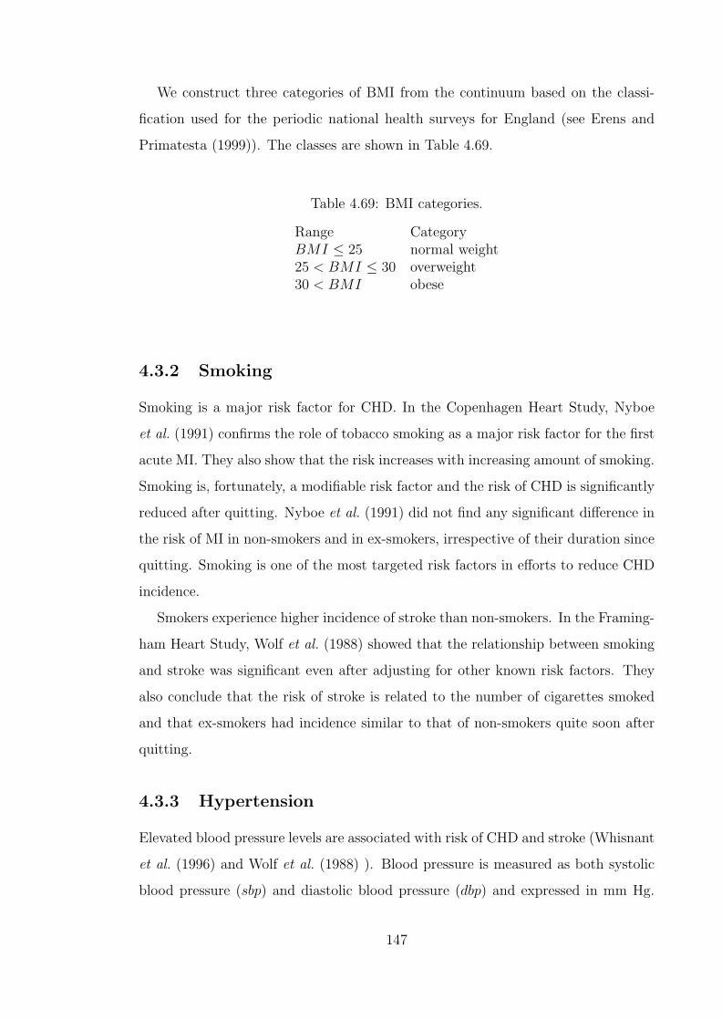
We construct three categories of BMI from the continuum based on the classi-
fication used for the periodic national health surveys for England (see Erens and
Primatesta (1999)). The classes are shown in Table 4.69.
Table 4.69: BMI categories.
Range CategoryBMI ≤ 25 normal weight25 < BMI ≤ 30 overweight30 < BMI obese
4.3.2 Smoking
Smoking is a major risk factor for CHD. In the Copenhagen Heart Study, Nyboe
et al. (1991) confirms the role of tobacco smoking as a major risk factor for the first
acute MI. They also show that the risk increases with increasing amount of smoking.
Smoking is, fortunately, a modifiable risk factor and the risk of CHD is significantly
reduced after quitting. Nyboe et al. (1991) did not find any significant difference in
the risk of MI in non-smokers and in ex-smokers, irrespective of their duration since
quitting. Smoking is one of the most targeted risk factors in efforts to reduce CHD
incidence.
Smokers experience higher incidence of stroke than non-smokers. In the Framing-
ham Heart Study, Wolf et al. (1988) showed that the relationship between smoking
and stroke was significant even after adjusting for other known risk factors. They
also conclude that the risk of stroke is related to the number of cigarettes smoked
and that ex-smokers had incidence similar to that of non-smokers quite soon after
quitting.
4.3.3 Hypertension
Elevated blood pressure levels are associated with risk of CHD and stroke (Whisnant
et al. (1996) and Wolf et al. (1988) ). Blood pressure is measured as both systolic
blood pressure (sbp) and diastolic blood pressure (dbp) and expressed in mm Hg.
147
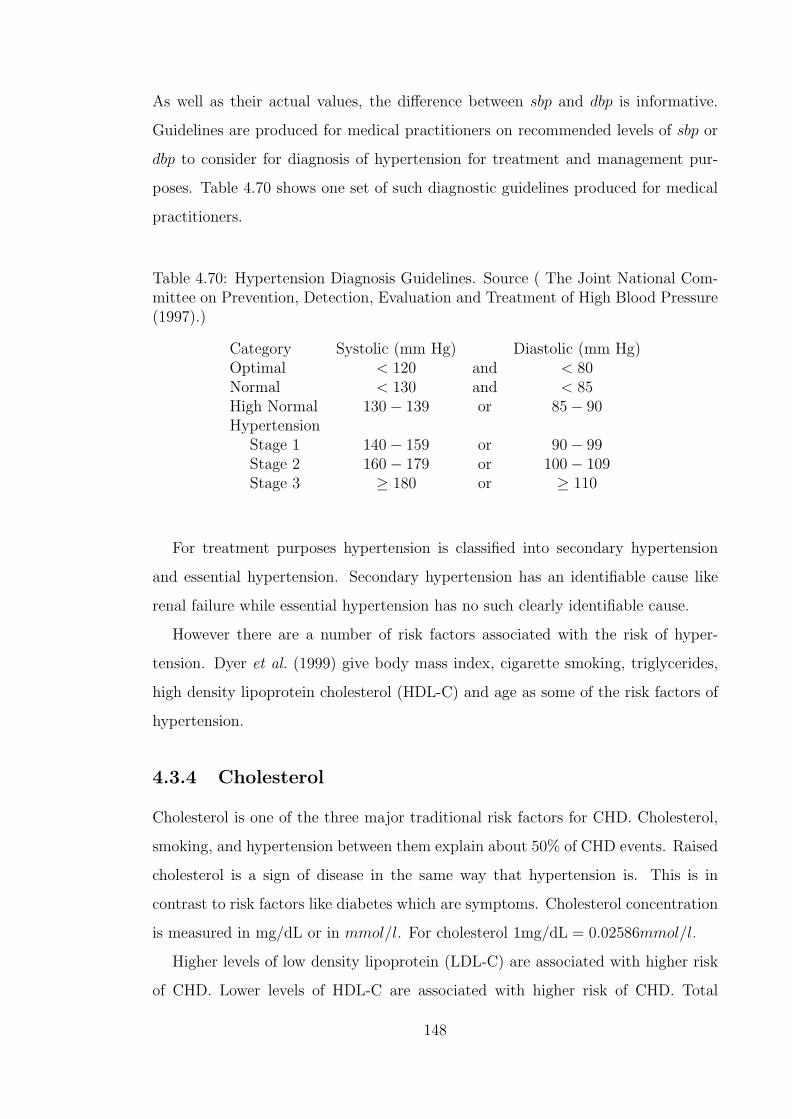
As well as their actual values, the difference between sbp and dbp is informative.
Guidelines are produced for medical practitioners on recommended levels of sbp or
dbp to consider for diagnosis of hypertension for treatment and management pur-
poses. Table 4.70 shows one set of such diagnostic guidelines produced for medical
practitioners.
Table 4.70: Hypertension Diagnosis Guidelines. Source ( The Joint National Com-mittee on Prevention, Detection, Evaluation and Treatment of High Blood Pressure(1997).)
Category Systolic (mm Hg) Diastolic (mm Hg)Optimal < 120 and < 80Normal < 130 and < 85High Normal 130− 139 or 85− 90Hypertension
Stage 1 140− 159 or 90− 99Stage 2 160− 179 or 100− 109Stage 3 ≥ 180 or ≥ 110
For treatment purposes hypertension is classified into secondary hypertension
and essential hypertension. Secondary hypertension has an identifiable cause like
renal failure while essential hypertension has no such clearly identifiable cause.
However there are a number of risk factors associated with the risk of hyper-
tension. Dyer et al. (1999) give body mass index, cigarette smoking, triglycerides,
high density lipoprotein cholesterol (HDL-C) and age as some of the risk factors of
hypertension.
4.3.4 Cholesterol
Cholesterol is one of the three major traditional risk factors for CHD. Cholesterol,
smoking, and hypertension between them explain about 50% of CHD events. Raised
cholesterol is a sign of disease in the same way that hypertension is. This is in
contrast to risk factors like diabetes which are symptoms. Cholesterol concentration
is measured in mg/dL or in mmol/l. For cholesterol 1mg/dL = 0.02586mmol/l.
Higher levels of low density lipoprotein (LDL-C) are associated with higher risk
of CHD. Lower levels of HDL-C are associated with higher risk of CHD. Total
148

Table 4.71: ATP III Classification of LDL, Total and HDL Cholesterol (mg/dL)Source ( National Cholesterol Education Program (2001).)
LDL Cholesterol< 100 Optimal
100− 129 Near optimal/above optimal130− 159 Borderline high160− 189 High≥ 190 Very high
Total Cholesterol< 200 Desirable
200− 239 Borderline high≥ 240 High
HDL Cholesterol< 40 Low≥ 60 High
cholesterol (TC) levels measure the combined total level of LDL cholesterol and
HDL cholesterol and triglycerides. It is now felt that a measure of the ratio of LDL
cholesterol to HDL cholesterol ( LDLHDL
) is more powerful in explaining CHD than the
total cholesterol levels. We note that often the LDL value is not known and the
ratio ( TCHDL
) is used in its place.
For diagnosis and treatment purposes the National Cholesterol Education Pro-
gram (2001) give the classification of cholesterol levels shown in Table 4.71.
Continuing research into the CHD risk factors often redefines the importance of
traditional risk factors as new ones are found. We note here that Brackenridge and
Elder (1998) refer to LDL-C as a new independent risk factor for CHD
There seems to be no consistent result from epidemiological studies on whether
cholesterol is a risk factor for stroke or not. In a study of 7052 men and 8354 women
who had baseline examination in the mid-1970’s when they were then aged 45 to
64 years, Hart et al. (2000) failed to find a relationship between cholesterol and
stroke incidence. This was true for both men and women considering a follow-up
period of up to 20 years. Dyker et al. (1997) points out that some studies find that
cholesterol has positive association with ischaemic stroke and a negative association
149

with haemorrhagic stroke and that it is likely that when stroke is studied without
subdividing the subtypes, the influence of cholesterol is diluted.
4.3.5 Diabetes
The presence of elevated glucose levels in the blood (glycaemia) is associated
with CHD risk. Epidemiological studies have shown that diabetes is also asso-
ciated with risk of stroke (Whisnant et al. (1996)). The level of glucose in the
blood is measured as either the plasma glucose (PG) level or the glycosylated
haemoglobin (HbA1c) concentration. The plasma glucose level is expressed in
mg/dL (or mmol/l) and HbA1c is expressed as a percentage. For blood glucose
level 1mg/dL = 0.05556mmol/l. The blood glucose level is a continuum over the
ranges of measurement compatible with life, and varies through the day in response
to meals and exercise.
The glycaemia continuum is categorised into two main groups. The normo-
glycaemic range on the lower end of the scale and hyperglycaemic on the upper
end of the scale. The lower end of the hyperglycaemic part forms the Impaired Glu-
cose Tolerance (IGT) or Impaired Fasting Glucose (IFG) category while the upper
end forms the Diabetic category. This is shown in Figure 4.28.
-¾ ¾ -Normoglycaemic Hyperglycaemic
-¾ ¾ -¾ -Normal IFG or IGT Diabetic
Figure 4.28: The Glycaemia continuum.
The Expert Committee on the Diagnosis and Classification of Diabetes Mellitus,
set up by the American Diabetes Association (see American Diabetes Association:
Clinical Practice Recommendations 2000 (2000)), gave guidelines on the glycaemia
ranges constituting the above categories. To achieve this they define the conditions
for measuring the plasma glucose level such as, the casual plasma glucose level, the
fasting plasma glucose (FPG) level and the 2 hour postload glucose level (2-h PG).
150
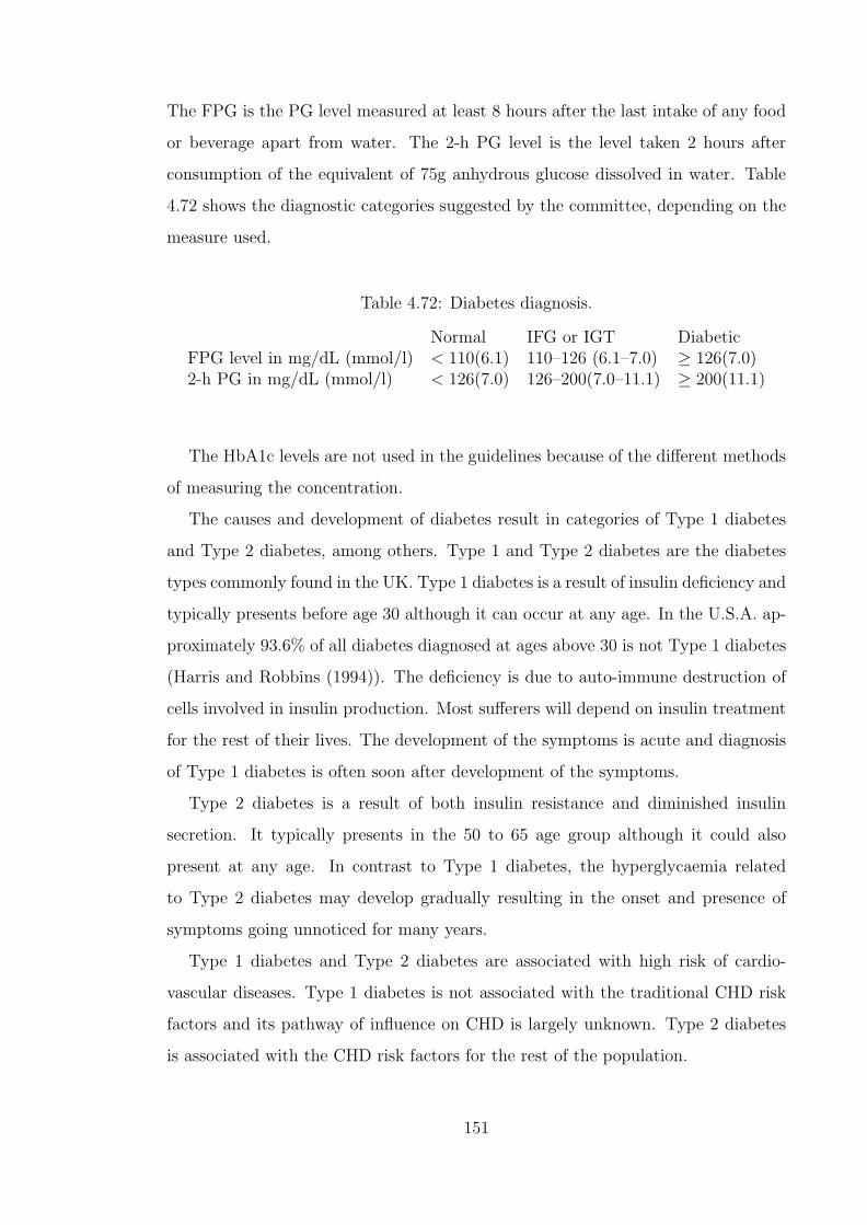
The FPG is the PG level measured at least 8 hours after the last intake of any food
or beverage apart from water. The 2-h PG level is the level taken 2 hours after
consumption of the equivalent of 75g anhydrous glucose dissolved in water. Table
4.72 shows the diagnostic categories suggested by the committee, depending on the
measure used.
Table 4.72: Diabetes diagnosis.
Normal IFG or IGT DiabeticFPG level in mg/dL (mmol/l) < 110(6.1) 110–126 (6.1–7.0) ≥ 126(7.0)2-h PG in mg/dL (mmol/l) < 126(7.0) 126–200(7.0–11.1) ≥ 200(11.1)
The HbA1c levels are not used in the guidelines because of the different methods
of measuring the concentration.
The causes and development of diabetes result in categories of Type 1 diabetes
and Type 2 diabetes, among others. Type 1 and Type 2 diabetes are the diabetes
types commonly found in the UK. Type 1 diabetes is a result of insulin deficiency and
typically presents before age 30 although it can occur at any age. In the U.S.A. ap-
proximately 93.6% of all diabetes diagnosed at ages above 30 is not Type 1 diabetes
(Harris and Robbins (1994)). The deficiency is due to auto-immune destruction of
cells involved in insulin production. Most sufferers will depend on insulin treatment
for the rest of their lives. The development of the symptoms is acute and diagnosis
of Type 1 diabetes is often soon after development of the symptoms.
Type 2 diabetes is a result of both insulin resistance and diminished insulin
secretion. It typically presents in the 50 to 65 age group although it could also
present at any age. In contrast to Type 1 diabetes, the hyperglycaemia related
to Type 2 diabetes may develop gradually resulting in the onset and presence of
symptoms going unnoticed for many years.
Type 1 diabetes and Type 2 diabetes are associated with high risk of cardio-
vascular diseases. Type 1 diabetes is not associated with the traditional CHD risk
factors and its pathway of influence on CHD is largely unknown. Type 2 diabetes
is associated with the CHD risk factors for the rest of the population.
151

We note that on the one hand there is increased incidence of Type 2 diabetes
in people with obesity, older ages, sedentary lifestyles, family history of diabetes,
hypertension and dyslipidaemia (American Diabetes Association: Clinical Practice
Recommendations 1999 (1999)). On the other hand people with Type 2 diabetes
are more likely to have these risk factors (apart from LDL-C and smoking) than age
matched non-diabetics (Nathan et al. (1997)). Type 2 diabetics are also more likely
to have clustering of these risk factors than non-diabetics.
For those with Type 2 diabetes, Turner et al. (1998) show that LDL-C, HDL-C,
smoking and hypertension ( > 160/90 mm Hg) remain risk factors for CHD while
obesity is not. It is also true that in general, Type 2 diabetics tend to develop CHD
earlier with worse prognosis than non-diabetics.
Studies are not in agreement on the relationship between glycaemia and CHD
risk in Type 2 diabetics. Some studies suggest that the treatment of diabetes does
not seem to reduce CHD risk (Tan (1999)).
The normal end of the glycaemic scale is associated with the lowest risk of CHD.
Glycaemia levels in the IGT or IFG states, although not high enough to constitute
diabetes, are associated with higher CHD risk than the normal range. This could
be considered as midway between the normal and diabetes associated risks.
Diabetes is also associated with peripheral vascular disease (PVD) which is due
to hardening of arteries with effects mainly in the legs. PVD is not a CI claim
trigger but lives with PVD are declined CI insurance cover. In our modelling we
consider diabetes, which is a risk factor for CHD rather than PVD which is just an
indication that the individuals arteries are not healthy.
4.4 CHD and stroke underwriting for CI insur-
ance
With respect to quantitative risk factors associated with CHD, Sing and Moll (1990)
state that there is no level of these factors at which risk of CHD is totally absent or
an absolute certainty. Consequently everyone is at some risk of CHD or stroke.
152

The underwriting of CI insurance has some specific focus on CHD and stroke and
their risk factors. It should be borne in mind that the underwriting is done for the
complete CI policy and not just for CHD and stroke outcomes. However particular
attention is paid to all the risk factors mentioned above and also to the applicant’s
own history of CHD or stroke. This is so mainly because the cardiovascular CI claim
events form a significant proportion of claims.
Applicants who have a history of any of the CI insurance claim events are unlikely
to be accepted for CI insurance cover. However if the applicant can be accepted at
non-standard rates which include an exclusion of claims due to diseases already
covered, then this may be done. Current practice is such that applicants with a
history of heart attacks, stroke and other atherosclerotic disease will be declined CI
cover.
The family history considered is the presence of family members with a history
of, or deceased from, diseases of the heart, diseases of the blood vessels or diabetes.
An adverse family history is likely to trigger more medical investigations. In some
cases, if the risk profile in terms of the other risk factors is good, standard rates may
still be offered. Typical ratings associated with adverse family history range from
+50 to +100.
Diabetes is considered one of most the important underwriting factors for CI
insurance. Apart from its association with cardiovascular diseases, diabetes also is
a risk factor for kidney disease. Current underwriting practice considers the age of
the applicant, the prognosis of the diabetes since it was diagnosed and the results
of tests related to possible complications of diabetes. These tests are likely to cover
aspects such as signs of affected kidneys. An applicant with a history of diabetes
will be declined if the diabetes has not been well controlled by treatment. They are
also likely to be declined if they are below 40 at age of diagnosis. Otherwise ratings
ranging from +50 to +150 can be offered just on the basis of diabetes being present.
We note that this practice is based on a criterion of diagnosis which considers a
blood sugar level of about 140mg/dL as the threshold for diagnosis.
Hypercholesterolaemia is also considered in CI insurance underwriting. The basic
measure used in underwriting is the blood concentration of total cholesterol and the
153

age of the applicant. Concentrations of up to 240mg/dL would typically not be rated.
For applicants above age 50 standard terms may be offered even for concentrations as
high as 300mg/dL while these concentrations for lives below 50 may attract ratings
of up to +75. In cases where the HDL-cholesterol values are available, these are also
used.
The consideration given to blood pressure readings in CI underwriting depends
on the level of the blood pressure and the age and sex of applicant. Values of
both the systolic blood pressure and the diastolic blood pressure are usually used
in the assessment. Most applicants are likely to have readings which can lead to
standard terms being offered. However the ratings for hypertension alone can lead
to declinature.
As already shown, the age of the applicant is a factor considered in CI insurance
underwriting. The sex and smoking status are also considered. The ratings given
are based on the appropriate standard premium specific to the sex, age and smoking
status of the applicant. Therefore the standard premium paid by male smokers will
be different to the standard premium paid by female smokers. Consequently the
same applies to the rated premiums. The ratings used are assumed to have more
than just an additive effect. If three risk factors have individual ratings whose sum
is +100, then the rating for the presence of all three is in excess of +100.
Body mass index is considered a minor risk factor in terms of CI insurance under-
writing. Considered on its own it is will to lead to the declinature of an application
only if the BMI is above 40. For BMI below 40 the ratings may depend on the age
of the applicant with applicants at older ages getting lower ratings than younger
lives with the same BMI.
4.5 The genetics of CHD and stroke
The genetics of CHD or stroke is a large and complex subject of study. We note here
that the accepted facts are that cardiovascular disorders aggregate in families but do
not exhibit the pattern of inheritance shown by single gene disorders (segregation).
Sing and Moll (1990) state that, with reference to coronary artery disease, this is
154

expected if:
(a) the disease is determined by the levels of many intermediate quantitative traits
and
(b) the distribution of these quantitative traits is influenced by the segregation of
many genes and environmental factors.
There is an expectation that there would be a few rare single gene mutations,
associated with the risk factors, that would predict CHD with high probability.
However in general there is no such clear relationship between the DNA mutations
and disease status. Therefore the research into the genetics of these complex disor-
ders has been mainly on the genes that may cause the inter-individual variation in
the intermediate quantitative traits.
We will consider some of the advances in the genetics of hypertension, hyperc-
holesterolaemia and diabetes. The aim of geneticists in the study of the genetics
of these intermediate traits is to establish the ‘genetic architecture’, (Sing and Moll
(1990)), which includes
(a) the number of genes involved in determining the level and inter-individual vari-
ation of the trait,
(b) the number of alleles of each gene and their relative frequencies,
(c) the impact of each allele on the level of variability of the trait, and
(d) the impact of each allele on the relationship of the trait with other risk factors
that are involved in the development of the disease.
When more that one gene is involved, a gene whose influence on the inter-
individual variation of the trait is much greater than the influence of modifying
genes is referred to as a major gene.
4.5.1 Hypertension
Some rare single gene mutations have been identified which are associated with
hypertension. Examples of these rare or extremely rare mutations given by Corvol
et al. (1999) are the genes on chromosome 16 leading to the kidney disorder Liddle’s
syndrome and also genes on chromosomes 8 and 16.
155
A lot of attention has been paid to more common mutations that may be linked
to hypertension. The first one to be linked to human hypertension (and maybe the
most studied one) is the AGT gene on chromosome 1. Its polymorphisms include the
2 frequent alleles M235T and T174M. Studies in different populations have shown
differing results on the association between the gene and hypertension. However, as
Corvol et al. (1999) note two meta-analyses in the late 1990’s showed a weak but
significant association between the M235T allele and hypertension.
Other common genes being considered as candidate genes for hypertension in-
clude the NOS3 gene on chromosome 7 (Robinson et al. (1994)) and the GNB3 gene
on chromosome 12 (Benjafield et al. (1998)). These are known genes whose associ-
ation with hypertension is being studied. There are also some loci which possibly
harbour hypertension susceptibility genes. These include the HYT1 locus on chro-
mosome 17 (Baima et al. (1999)) and the HYT2 locus on chromosome 15 (Xu et al.
(1999)).
4.5.2 Hypercholesterolaemia
A few rare single gene mutations have been associated with cholesterol disorders.
An example of these is familial hypercholesterolemia, (FH), which is an autosomal
dominant disorder whose sufferers have very high levels of serum cholesterol. FH
is caused by mutations at the LDL receptor gene, LDLR, on chromosome 19. One
such mutation which occurs with a frequency of 1 in 500 gives rise to risk of a
CHD event of 50% by age 50 in males (see Motulski and Brunzell (1992)). Two
other mutations at the LDL receptor gene with frequency 1 in 1,000,000 can result
in levels of cholesterol of up to 600 mg/dl (≈ 15.5 mmol/l). The Human Gene
Mutation Database showed the number of different known mutations of the LDL
receptor gene as 441. The elevated cholesterol levels associated with FH can be
detected by the analysis of a blood sample. The cholesterol levels are elevated from
birth and FH does not skip generations. Therefore a genetic test gives very limited
information in addition to that obtained from a blood test.
The apo E gene, also on chromosome 19, is an example of the common genes as-
sociated with cholesterol disorders. Apo E is found in 3 isoforms, ε2, ε3, and ε4. The
156

resulting six genotypes are ε2/ε2, ε2/ε3, ε2/ε4, ε3/ε3, ε3/ε4, ε4/ε4. As compared to
carriers of the ε2 allele, those with the ε4 allele have higher atherosclerosis risk. The
ε4 allele is associated with higher cholesterol, higher LDL-cholesterol, higher Lp(a),
higher triglycerides and lower HDL-cholesterol than ε3 (Dallongenville (1994)). The
effect of the polymorphisms on the cholesterol levels is also influenced by environ-
mental factors like the level of cholesterol in the diet. The apo E gene is also mainly
associated with late-onset Alzheimer’s disease. Lives with the ε4 allele are at greater
risk of late-onset Alzheimer’s disease but many lives with the ε4 allele do not get
the disease while many without the allele develop the disease. Therefore apo E
genotyping is not a reliable predictive test for hypercholesterolaemia or late-onset
Alzheimer’s disease. The determination of the apo E genotype is not usually done
in individuals (Motulski and Brunzell (1992)).
With respect to LDL-C, Coon et al. (1999) found evidence of a common gene
associated with mild elevations of LDL-C. However candidate genes like the LDL
receptor gene, the apo E gene and CYP7A1 were excluded by the studies. A major
gene has also been suggested to regulate HDL-C levels. Candidate genes have been
considered but none has been accepted as the major gene. Recent study results
include evidence that some regions of chromosomes 5 and 13 may harbour a gene
that influences the inter-individual variation in HDL-C ( Peacock et al. (2001)).
4.5.3 Diabetes
Genetics of Type 1 diabetes
Type 1 diabetes runs in families so that the offspring and siblings of diabetics have
a much higher chance of being diabetics than the general population. Multiple loci
may be involved in the disease process as well as environmental factors and a number
of loci have been considered as candidate genes contributing to Type 1 diabetes
(Rotter et al. (1992)). The region considered as primary for Type 1 diabetes is on
chromosome 6 named IDDM1 (Dorman and Bunker (2000)). IDDM1 is part of the
human leukocyte antigen (HLA) complex and comprises the loci HLA-DR, HLA-DQ
and HLA-DP. Some HLA alleles are believed to predispose to Type 1 diabetes. In
particular lives with both DR3 and DR4 alleles have a higher relative risk of Type 1
157
diabetes than lives which are homozygous for either DR3 or DR4. While initial focus
was on the DR alleles as markers for type 1 diabetes susceptibility, recent studies
have established the DQ alleles as the primary markers (Dorman and Bunker (2000)
and Rotter et al. (1992)). Davies et al. (1994) state that the number of siblings
with similar specific HLA haplotypes is far higher among diabetes sufferers than
would be expected from Mendelian genetics. IDDM1 is thought to be the gene with
the largest contribution to Type 1 diabetes. A gene on chromosome 11, named
IDDM2, is also thought to predispose to Type 1 diabetes. IDDM1 and IDDM2 are,
together, thought to account for less than 30% of genetic susceptibility to Type 1
diabetes. The pattern of inheritance of these genes is complex. This complexity may
be increased if there is selective transmission of particular alleles by the parents (see
Vadheim et al. (1986) and Field et al. (1986)).
Genetics of Type 2 diabetes
There is a high incidence of Type 2 diabetes in certain populations and in relatives of
Type 2 diabetes patients. These and other facts, including the high concordance in
identical twins, is taken as evidence of a strong genetic influence on Type 2 diabetes.
In recent years researchers have identified a number of gene loci with evidence
of influence on Type 2 diabetes. In 1996, Hanis et al. (1996) identified NIDDM1
on chromosome 2. Loci NIDDM2 on chromosome 12, and NIDDM3 on chromosome
20 were identified in 1996 and 1999 respectively. On the NIDDM1 locus, Horikawa
et al. (2000) concluded that genetic variation on the CAPN10 gene (segment 2q37.3)
is associated with type 2 diabetes.
Frayling et al. (2000) discussed the difficulties of identifying genes associated
with Type 2 diabetes. The problems include having different genes contributing in
different individuals, the possibility of multiple susceptibility alleles for each affected
subject, and the role of environmental factors. There have also been difficulties in
reproducing results in different populations. Frayling et al. (2000) failed to reproduce
the results on chromosomes 12 and 20 for U.K. Caucasians while Evans et al. (2001)
failed to reproduce the CAPN10 gene results in the U.K. However the setting up,
in 1997, of the International Type 2 Diabetes Linkage Analysis Consortium should
158

increase the pace at which identification of genes is achieved.
As expected the epidemiology of diabetes in lives with any mutation will follow
behind the identification of the relevant genes. Our search of the literature did not
reveal what, in quantitative terms, the incidence of type 2 diabetes in mutation
carriers is expected to be in relation to that in non-mutation carriers. Neither did
we get an idea about the frequencies of any such possible mutation or mutations.
Our discussion of the genetics of cardiovascular endpoints show the difficulties
in establishing a clear link between DNA mutations and the endpoints. We had
such a reasonable link in our work on BCOC. The discussion also shows that it may
be some time until any genetic architecture that can be useful for epidemiological
analysis is available. To bring our research goals of analysing the effects of genetics
on insurance to reasonable success, we will start by attempting to construct models
for the development of the cardiovascular endpoints that take explicit account of
the development of the intermediate quantitative or factor traits in the absence of
any genetic knowledge. This will allow us to assess the impact of some hypothetical
genetic effects by adjusting the intermediate traits. By making assumptions of
genetic effects on the intermediate traits which can be shown to be extreme, we can
get estimates of the bounds of the impact of genetic information on insurance costs.
4.6 Models for the development of CHD, stroke
and the risk factors
We intend to construct a model which is an adaptation of Figure 4.27 so as to
(a) incorporate the risk factors diabetes, hypertension and hypercholesterolaemia
as proxy for underlying atherosclerosis, and
(b) consider CHD (defined as MI only) as one distinct endpoint and stroke as a
separate endpoint.
Our efforts to construct and parameterize the model will be guided largely by
the data recorded in the Framingham Heart Study and to a lesser extent by other
sources of data and guidelines. The Framingham study was conducted in Boston
(Massachusetts, U.S.A) by the National Heart, Lung and Blood Institute, starting
159
in the late 1940’s and running up to the present day.
4.6.1 The Framingham Heart Study data
Available to us is data pertaining to the original cohort of 5209 (2336 men and
2873 women) participants. These people were aged between 28 and 62 years when
they attended their first study examination. Participants were then monitored by
bi-annual examinations for up to forty years (21 examinations), stretching in time
to the early 1990’s. At these examinations details of the results of a range of med-
ical tests and blood analyses were recorded. Characteristics like weight, age and
height, among others, were recorded and the participants’ status with respect to
cardiovascular diseases was noted.
These data, together with another data set pertaining to the offspring of some
of the original cohort members (which we did not have during this work) have been
used to investigate models for the risk of cardiovascular diseases. Models developed
include those which estimate the probability of cardiovascular events within up to
twelve years from a baseline examination (see Anderson et al. (1991a) and Anderson
et al. (1991b)). They consider the time to event since the start of follow up as a
random variable and use parametric regression to estimate probabilities of disease
within a specified time, given the levels of risk factors at baseline. We note that
Anderson et al. (1991a) and Anderson et al. (1991b) consider variables like blood
pressure and cholesterol as continuous variables but diabetes is considered as a
discrete variable. Wilson et al. (1998) produced a model in which the risk factors
blood pressure and cholesterol were considered as categories rather than continuous
variables. These models have been widely used to construct cardiovascular risk
tables and risk calculators. The success of these models can also be shown by
the fact that guidelines on the diagnosis of hypertension and hypercholesterolaemia
now recommend partly on the basis of the CHD risk (according to these models)
of specific blood pressure and cholesterol levels (The Joint National Committee on
Prevention, Detection, Evaluation and Treatment of High Blood Pressure (1997),
Ramsay et al. (1999), and National Cholesterol Education Program (2001)).
160

However due to the fact that these models estimate the probabilities of cardio-
vascular events, they do not fall neatly into the framework of the continuous time
multiple state models introduced in Section 1.3 for which transition intensities rather
than probabilities are used in the model specification. We note that it is possible,
albeit difficult, to derive a set of transition intensities which may be reasonably
consistent with the probabilities given by the models of Anderson et al. (1991a) and
Anderson et al. (1991b). The difficulty arises from the following: Anderson et al.
(1991a) and Anderson et al. (1991b) state that the time to event for which a prob-
ability is estimated using their models should not be less than four years. Now the
probability of a cardiovascular event within, say, 5 years of baseline is a sum of
(a) the probability that an event occurs within 5 years with no change of risk factors
between baseline and time of event, and
(b) the probabilities that an event occurs within 5 years after any possible change
in the level of risk factors between baseline and time of event.
Even in the cases where risk factors are discrete, this means the probability of an
event is a sum of many composite probabilities, most of which include probabilities
of changing the risk factor levels. Therefore to use the Anderson et al. (1991a) and
Anderson et al. (1991b) probabilities to derive transition intensities requires making
assumptions about the models governing the change in the level of risk factors in an
individual. Another consequence of attempting to derive the transition intensities
in this way is that two individuals with the same levels of risk factors but different
durations with the risk factors could have significantly different transition intensi-
ties. This duration dependence of cardiovascular risk may not be readily supported
by medical opinion and does not fall within the Markov framework in which we
want to develop our model. Our investigations based on the Anderson et al. (1991a)
and Anderson et al. (1991b) probabilities show that while it is possible to remove
the duration dependency of the transition intensities, for example by averaging in-
tensities whose durations are different, the transition intensities produced will give
results which may be significantly different from those of the probability models
from which they are derived.
161

Influenced by these difficulties of using the probability models to parameterise a
multiple state Markov model and also by our desire to produce a model which not
only captures the development of cardiovascular disease but also the development,
enroute, of the risk factors blood pressure, diabetes and hypercholesterolaemia, we
feel that direct analysis of the Framingham Heart Study data set is the most appro-
priate approach.
The data
For the participants who attended a particular examination, Table 4.73 gives a sum-
mary of the data available on the factors that we are going to use. These data were
made available on the Public Release Data Tapes and excludes some information
which was collected in the study and possibly available to other studies such as
Anderson et al. (1991a) and Anderson et al. (1991b). There is more data and for a
greater range of ages for the earlier examinations than for the later examinations.
Table 4.73: Summary of data available from Framingham Heart Study.
ExaminationsFactors 1 2 3 4 5 6 7 8 9 10Smoking • • • • • • •Blood Sugar Level • • • • • • • •Serum Cholesterol • • • • • • • • •Systolic Blood Pressure • • • • • • • • • •Diastolic Blood Pressure • • • • • • • • • •Height • •Weight • • • • • • • • • •
ExaminationsFactors 11 12 13 14 15 16 17 18 19 20Smoking • • • • • • • • •Blood Sugar level • • • • • • • • •Serum Cholesterol • • •Systolic Blood Pressure • • • • • • • • • •Diastolic Blood Pressure • • • • • • • • • •Height • • • • • • • •Weight • • • • • • • • • •
The date at which a participant attended an examination is given. These dates
are provided only as the number of days from a fixed date in time. This fixed date
162

is not provided and we assume that it is 1 January 1960. Based on details collected
at these examinations and on other information, the data sets provide dates at
which vital events like a heart attack, stroke or death occur. Unlike the dates of
examinations, the dates pertaining to these events are given as actual calendar dates.
We consider the period between any two consecutively numbered examinations as
a separate period of investigation. For each applicant we determine the following
variables for the period of investigation:
(a) Calendar time. This denotes the time passed, at the start of the period of
investigation, since examination 1. We assume that all examinations are exactly
two years apart for this purpose. We define a variable e = 2(n− 1) where n is
the number of the examination.
(b) Start of investigation period. This is the date at which the current exami-
nation is attended by the participant. We define the variable date(0) to represent
this date.
(c) End of investigation period. This is the date of the next numbered ex-
amination, if it is attended. We denote this date(1) and we assume that
date(1) = date(0) + 2 if the participant does not attend the examination (i.e
if date(1) is not given).
(d) Sex. This is recorded for each participant at examination 1. We define the
variable s such that s = 0 for males and s = 1 for females.
(e) Age (denoted x). Age is recorded when the participant attended an examina-
tion. This recorded age is the age last birthday and therefore lives recorded
as aged y at start of the period have an average age of y + 0.5 years. Midway
through the two year period of investigation the average age of these lives is
y + 1.5 years. We define x = y + 1.5.
(f) Smoking status. This is taken to be the status recorded when the participant
took the examination. The Framingham study defined this in such a way that
one is classified a smoker if they smoked cigarettes within a year prior to the
examination. If the smoking status is not recorded at the examination under
consideration we assumed the status at the last recorded examination. We define
the variable k such that k = 0 for non-smokers and k = 1 for smokers.
163
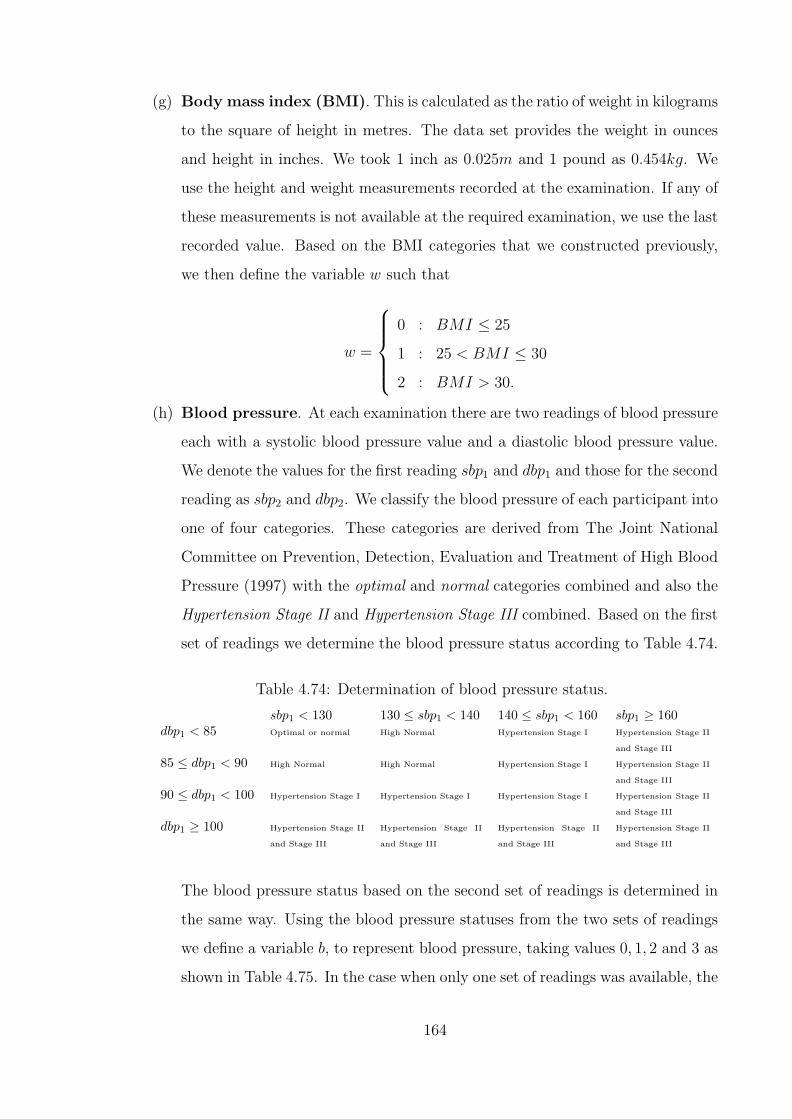
(g) Body mass index (BMI). This is calculated as the ratio of weight in kilograms
to the square of height in metres. The data set provides the weight in ounces
and height in inches. We took 1 inch as 0.025m and 1 pound as 0.454kg. We
use the height and weight measurements recorded at the examination. If any of
these measurements is not available at the required examination, we use the last
recorded value. Based on the BMI categories that we constructed previously,
we then define the variable w such that
w =
0 : BMI ≤ 25
1 : 25 < BMI ≤ 30
2 : BMI > 30.
(h) Blood pressure. At each examination there are two readings of blood pressure
each with a systolic blood pressure value and a diastolic blood pressure value.
We denote the values for the first reading sbp1 and dbp1 and those for the second
reading as sbp2 and dbp2. We classify the blood pressure of each participant into
one of four categories. These categories are derived from The Joint National
Committee on Prevention, Detection, Evaluation and Treatment of High Blood
Pressure (1997) with the optimal and normal categories combined and also the
Hypertension Stage II and Hypertension Stage III combined. Based on the first
set of readings we determine the blood pressure status according to Table 4.74.
Table 4.74: Determination of blood pressure status.
sbp1 < 130 130 ≤ sbp1 < 140 140 ≤ sbp1 < 160 sbp1 ≥ 160dbp1 < 85 Optimal or normal High Normal Hypertension Stage I Hypertension Stage II
and Stage III
85 ≤ dbp1 < 90 High Normal High Normal Hypertension Stage I Hypertension Stage II
and Stage III
90 ≤ dbp1 < 100 Hypertension Stage I Hypertension Stage I Hypertension Stage I Hypertension Stage II
and Stage III
dbp1 ≥ 100 Hypertension Stage II
and Stage III
Hypertension Stage II
and Stage III
Hypertension Stage II
and Stage III
Hypertension Stage II
and Stage III
The blood pressure status based on the second set of readings is determined in
the same way. Using the blood pressure statuses from the two sets of readings
we define a variable b, to represent blood pressure, taking values 0, 1, 2 and 3 as
shown in Table 4.75. In the case when only one set of readings was available, the
164
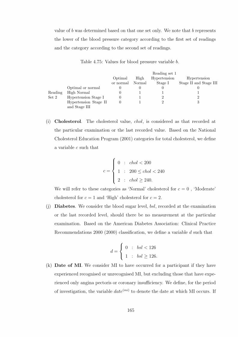
value of b was determined based on that one set only. We note that b represents
the lower of the blood pressure category according to the first set of readings
and the category according to the second set of readings.
Table 4.75: Values for blood pressure variable b.
Reading set 1Optimal High Hypertension Hypertension
or normal Normal Stage I Stage II and Stage IIIOptimal or normal 0 0 0 0
Reading High Normal 0 1 1 1Set 2 Hypertension Stage I 0 1 2 2
Hypertension Stage IIand Stage III
0 1 2 3
(i) Cholesterol. The cholesterol value, chol, is considered as that recorded at
the particular examination or the last recorded value. Based on the National
Cholesterol Education Program (2001) categories for total cholesterol, we define
a variable c such that
c =
0 : chol < 200
1 : 200 ≤ chol < 240
2 : chol ≥ 240.
We will refer to these categories as ‘Normal’ cholesterol for c = 0 , ‘Moderate’
cholesterol for c = 1 and ‘High’ cholesterol for c = 2.
(j) Diabetes. We consider the blood sugar level, bsl, recorded at the examination
or the last recorded level, should there be no measurement at the particular
examination. Based on the American Diabetes Association: Clinical Practice
Recommendations 2000 (2000) classification, we define a variable d such that
d =
0 : bsl < 126
1 : bsl ≥ 126.
(k) Date of MI. We consider MI to have occurred for a participant if they have
experienced recognised or unrecognised MI, but excluding those that have expe-
rienced only angina pectoris or coronary insufficiency. We define, for the period
of investigation, the variable date(mi) to denote the date at which MI occurs. If
165

MI does not occur during the period of investigation, then date(mi) takes the
value of infinity.
(l) Date of stroke. We considered a participant to have suffered a stroke if they
had an atherothrombotic infarction, cerebral embolism, intracerebral heamor-
rhage or subarachnoid haemorrhage, but excluding transient ischaemic attacks.
We define the variable date(stroke) to represent the date at which stroke occurs
during the period of investigation. date(stroke) takes the value infinity if the
participant does not experience a stroke during the period of investigation.
(m) Date of death. The variable date(dth) denotes the date of death and takes the
value infinity if the participant survives the period of investigation.
Based on the categories for the risk factors defined above we need to parameterise
the model for CHD and stroke shown in Figure 4.29. The states represent various
combinations of risk factors (as categorised above) as well as the events CHD (MI),
stroke and death. A life in any of the transient states numbered 1 to 23 can move
directly to the ‘CHD’, ‘Stroke’ or ‘Dead’ states. They may also move to another risk
factor state as shown by the arrows. The transition intensities between the states
depend on the risk factor status of the starting state. These transition intensities
will be defined and parameterised in the following sections of this chapter.
We use i to indicate the ith participant and define
dateexiti = minimum
(datedth
i , datemii , datestroke
i
).
The variables b for blood pressure, c for cholesterol and d for blood sugar level only
give information on the current levels. Indeed a significant proportion of lives would
have, at some previous examination, exceeded these levels of the variables. Using
details from the current and previous examinations, we define variables for the high-
est ever categories for blood pressure, cholesterol and blood sugar level. Therefore
we define bMax as the maximum value of b for the participant from examination 1
up to the current examination. Similarly we define dMax and cMax. For each of
blood pressure, cholesterol and blood sugar level we need to determine which one of
‘current value’ or ‘highest ever value’ is most informative in modelling MI or stroke
incidence. In the next section we detail the data, the model and the tests we use to
166

chol2diab9
?λbp01
¾¾¾
chol2bp1
??
10
λbp12
λdiab
???
bp1, diab
chol111
?
©©©©©©©©¼
λchol12 λbp12??? bp2
chol1
12
??
©©©©©©©©¼λchol12
λbp23
λdiab
??? bp2
diab
13
?
©©©©©©©©¼
λchol01
λbp23
???
bp314
--
-
?
©©©©©©©©¼λchol01 λdiab
bp1, diab
chol215
?λbp12
¾¾¾ bp2
chol2
16
?
@@
@@Rλdiab λbp23
???
bp2, diab
chol117
???
©©©©©©©©¼
HHHHHHHHjλbp23λchol12
bp3chol1
?
18
¡¡
¡¡ª
λdiabλchol12
??? bp3
diab
19
--
-
?λchol1
chol24
??
λdiab
λchol12
¾¾¾ diab
chol1
5
?
©©©©©©©©¼λbp01
λchol12???
chol1bp16
??
©©©©©©©©¼ λbp12
λdiab
λchol12
??? bp1
diab
7
?
©©©©©©©©¼λbp12
λchol01???
bp28
--
-
??
©©©©©©©©¼λbp23λdiabλchol01
chol11
-
-
-
? ?
HHHHHHHHjλchol12 λdiab λbp01
diab2
???
¡¡
¡¡ª
@@
@@Rλ
bp01λchol01
bp13
--
-
??
©©©©©©©©¼λbp12λdiab
λchol01
bp2, diab
chol220
¾¾¾
HHHHHHHHjλbp23
bp3chol2
21
?λdiab
???
bp3, diab
chol122
--
-
©©©©©©©©¼ λchol01
bp0chol00
¾
¾
¾
©©©©©©©©¼ ?
HHHHHHHHjλchol01 λdiab λbp01
bp3, diab
chol223
?λMI
x+t,s,w,b=3,d=1,c=2
--
CHD24 λMI
x+t,s,w,b,d,cλMIx+t,s,w,b,d,c
Stroke25 λStroke
x+t,s,k,b,dλStrokex+t,s,k,b,d
Dead26 λD
x+t,sλDx+t,s
Figure 4.29: A CHD and Stroke model.
167

make this determination. The notation used and expressions developed for the data
and models in the section will be referred to in later models.
4.6.2 Model for incidence of CHD and incidence of stroke
Assessment of the significance of blood pressure variables b and bMax
To model the incidence of MI/stroke we need to estimate the time spent at risk
of MI/stroke by the ith participant whose age (x), current blood pressure category
(b) and highest ever blood pressure category (bMax) are specified. We also need
to determine the number of MI cases (zero or one) for the same participant in the
period of investigation.
We consider three categories of participants:
(a) Participants who are present at the next numbered examination.
Since the date of the next examination is known, the exposure for the ith life is
given by
Ex,b,bMax,i = minimum(date(1)i , dateexit
i )− date(0)i .
Denoting by θx,b,bMax,i, the number of cases of MI/stroke for life i, we have
θMIx,b,bMax,i =
1 : dateexiti = dateMI
i and dateexiti <= date
(1)i
0 : otherwise,
and
θstrokex,b,bMax,i =
1 : dateexiti = datestroke
i and dateexiti <= date
(1)i
0 : otherwise.
(b) Participants who are not present at the next numbered examination but are
known to have had MI, stroke or death within 2 years of the date of the ex-
amination at the start of the investigation period.
For these participants there is no date(1)i available. The exposure and number
of cases for these lives are given by
168

Ex,b,bMax,i = dateexiti − date
(0)i .
θMIx,b,bMax,i =
1 : dateexiti = dateMI
i
0 : otherwise,
θstrokex,b,bMax,i =
1 : dateexiti = datestroke
i
0 : otherwise.
(c) Participants who are not present at the next numbered examination, did not
have any of MI, stroke or death within 2 years of the date of the examination
at the start of the investigation period and attended at least one of the three
examinations subsequent to the missed examination.
For these participants
Ex,b,bMax,i = 2
and
θMIx,b,bMax,i = θstroke
x,b,bMax,i = 0
We then define
Ex,b,bMax=
∑i
Ex,b,bMax,i as the exposed to risk
θMIx,b,bMax
=∑i
θMIx,b,bMax,i number of MI cases, and
θstrokex,b,bMax
=∑i
θstrokex,b,bMax,i number of stroke cases,
where the summation covers participants attending examinations 2 to 16 inclu-
sive. The ages considered are such that 30 ≤ x ≤ 82.
For MI we assume that
θMIx,b,bMax
∼ Poisson (Ex,b,bMax· exp (g(x, b, bMax)))
169

where g(·) is a linear predictor. To fit the linear predictor we have 490 data points.
We use a GLM which uses a stepwise fitting procedure and allows for possible inter-
actions between b and bMax. The fitting retains only age x and bMax as significant
variables. To illustrate why the choice of the stepwise fitting procedure is sensible we
show in Table 4.76 the residual deviance and degrees of freedom when we alternately
add bMax and b to the model.
Table 4.76: Model fitting for MI and stroke incidence considering covariates b (thecurrent blood pressure category) and bMax (the highest ever blood pressure cate-gory).
MI StrokeParameters in GLM Residual Degrees Residual Degreesmodel deviance of freedom deviance of freedomAge only 562 488 474 488Age and b only 498 485 370 485Age and bMax only 457 485 372 485Age, b and bMax 452 482 345 482
We conclude that bMax has more significance in MI prediction than b. We also
conclude that given bMax, b does not give us any more information on the MI in-
cidence. Table 4.76 also shows the results of a similar analysis with respect to the
incidence of stroke. In this case the results show that given either bMax or b in the
model, adding the other variable to the model gives a significant improvement in the
fitting. The results also show that b is slightly (maybe insignificantly) more infor-
mative of stroke incidence than bMax. We note that the stepwise fitting procedure
for the GLM retained both b and bMax as significant variables in the stroke incidence
model.
Assessment of the significance of cholesterol variables c and cMax
We calculate Ex,c,cMaxand θMI
x,c,cMaxin a way corresponding to that used to calculate
Ex,b,bMaxand θMI
x,b,bMax. We assume
θMIx,c,cMax
∼ Poisson (Ex,c,cMax· exp (g(x, c, cMax))) .
To fit the linear predictor, g(·), we have 293 data points. The GLM fit retains only
170
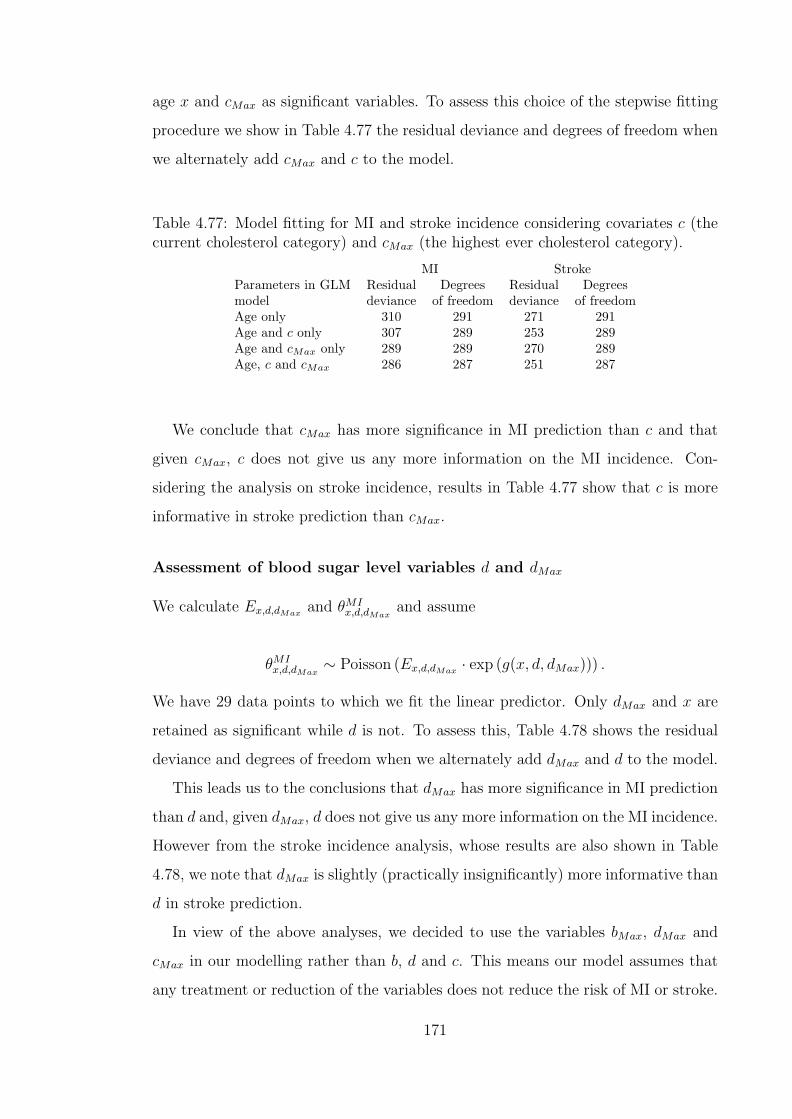
age x and cMax as significant variables. To assess this choice of the stepwise fitting
procedure we show in Table 4.77 the residual deviance and degrees of freedom when
we alternately add cMax and c to the model.
Table 4.77: Model fitting for MI and stroke incidence considering covariates c (thecurrent cholesterol category) and cMax (the highest ever cholesterol category).
MI StrokeParameters in GLM Residual Degrees Residual Degreesmodel deviance of freedom deviance of freedomAge only 310 291 271 291Age and c only 307 289 253 289Age and cMax only 289 289 270 289Age, c and cMax 286 287 251 287
We conclude that cMax has more significance in MI prediction than c and that
given cMax, c does not give us any more information on the MI incidence. Con-
sidering the analysis on stroke incidence, results in Table 4.77 show that c is more
informative in stroke prediction than cMax.
Assessment of blood sugar level variables d and dMax
We calculate Ex,d,dMaxand θMI
x,d,dMaxand assume
θMIx,d,dMax
∼ Poisson (Ex,d,dMax· exp (g(x, d, dMax))) .
We have 29 data points to which we fit the linear predictor. Only dMax and x are
retained as significant while d is not. To assess this, Table 4.78 shows the residual
deviance and degrees of freedom when we alternately add dMax and d to the model.
This leads us to the conclusions that dMax has more significance in MI prediction
than d and, given dMax, d does not give us any more information on the MI incidence.
However from the stroke incidence analysis, whose results are also shown in Table
4.78, we note that dMax is slightly (practically insignificantly) more informative than
d in stroke prediction.
In view of the above analyses, we decided to use the variables bMax, dMax and
cMax in our modelling rather than b, d and c. This means our model assumes that
any treatment or reduction of the variables does not reduce the risk of MI or stroke.
171
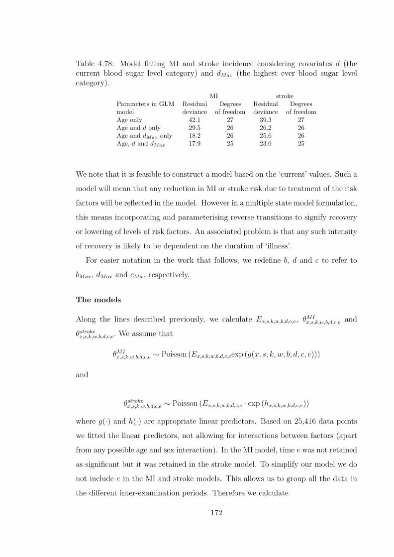
Table 4.78: Model fitting MI and stroke incidence considering covariates d (thecurrent blood sugar level category) and dMax (the highest ever blood sugar levelcategory).
MI strokeParameters in GLM Residual Degrees Residual Degreesmodel deviance of freedom deviance of freedomAge only 42.1 27 39.3 27Age and d only 29.5 26 26.2 26Age and dMax only 18.2 26 25.6 26Age, d and dMax 17.9 25 23.0 25
We note that it is feasible to construct a model based on the ‘current’ values. Such a
model will mean that any reduction in MI or stroke risk due to treatment of the risk
factors will be reflected in the model. However in a multiple state model formulation,
this means incorporating and parameterising reverse transitions to signify recovery
or lowering of levels of risk factors. An associated problem is that any such intensity
of recovery is likely to be dependent on the duration of ‘illness’.
For easier notation in the work that follows, we redefine b, d and c to refer to
bMax, dMax and cMax respectively.
The models
Along the lines described previously, we calculate Ex,s,k,w,b,d,c,e, θMIx,s,k,w,b,d,c,e and
θstrokex,s,k,w,b,d,c,e. We assume that
θMIx,s,k,w,b,d,c,e ∼ Poisson (Ex,s,k,w,b,d,c,eexp (g(x, s, k, w, b, d, c, e)))
and
θstrokex,s,k,w,b,d,c,e ∼ Poisson (Ex,s,k,w,b,d,c,e · exp (hx,s,k,w,b,d,c,e))
where g(·) and h(·) are appropriate linear predictors. Based on 25,416 data points
we fitted the linear predictors, not allowing for interactions between factors (apart
from any possible age and sex interaction). In the MI model, time e was not retained
as significant but it was retained in the stroke model. To simplify our model we do
not include e in the MI and stroke models. This allows us to group all the data in
the different inter-examination periods. Therefore we calculate
172

Ex,s,k,w,b,d,c =∑
e
Ex,s,k,w,b,d,c,e,
θMIx,s,k,w,b,d,c =
∑e
θMIx,s,k,w,b,d,c,e
and
θstrokex,s,k,w,b,d,c =
∑e
θstrokex,s,k,w,b,d,c,e.
This creates 6,981 data points and Table 4.79 shows summaries of the characteristics
of this data.
Table 4.79: Characteristics of data for MI and stroke models.
Variable Categories Exposure Cases(person years) MI Stroke
All 99032.2 581 304Sex s
Males 41301.1 405 142Females 57731.1 176 162
Smoking kNo 54873.3 289 180Yes 44158.9 292 124
Body Mass Index wNormal 34948.2 134 91Overweight 45021.8 303 131Obese 19062.2 144 82
Blood Pressure bOptimal or Normal 20477.9 34 19High Normal 18188.8 50 15Hypertension Stage I 29374.7 163 50Hypertension Stage II or III 30990.7 334 220
Diabetes dNo 88849.4 452 228Yes 10182.8 129 76
Cholesterol cNormal 7689.41 13 14Moderate 25102.5 96 62High 66240.2 472 228
MI
We fitted the data for males separately from that for females. In both cases we
found no significant difference in the coefficients for the blood pressure categories
b = 0 and b = 1 (that is between the ‘Optimal or Normal’ and the ‘High normal’
categories). We also did not find a significant difference between coefficients for the
cholesterol categories c = 0 and c = 1 (that is between the ‘Normal’ and ‘Moderate’
173
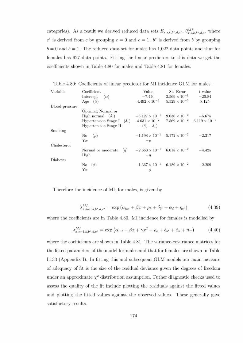
categories). As a result we derived reduced data sets Ex,s,k,b∗,d,c∗ , θMIx,s,k,b∗,d,c∗ where
c∗ is derived from c by grouping c = 0 and c = 1. b∗ is derived from b by grouping
b = 0 and b = 1. The reduced data set for males has 1,022 data points and that for
females has 927 data points. Fitting the linear predictors to this data we get the
coefficients shown in Table 4.80 for males and Table 4.81 for females.
Table 4.80: Coefficients of linear predictor for MI incidence GLM for males.
Variable Coefficient Value St. Error t-valueIntercept (α) −7.440 3.569× 10⁻¹ −20.84Age (β) 4.492× 10⁻² 5.529× 10⁻³ 8.125
Blood pressureOptimal, Normal orHigh normal (δ0) −5.127× 10⁻¹ 9.036× 10⁻² −5.675Hypertension Stage I (δ1) 4.631× 10⁻² 7.569× 10⁻² 6.119× 10⁻¹
Hypertension Stage II −(δ0 + δ1)Smoking
No (ρ) −1.198× 10⁻¹ 5.172× 10⁻² −2.317Yes −ρ
CholesterolNormal or moderate (η) −2.663× 10⁻¹ 6.018× 10⁻² −4.425High −η
DiabetesNo (φ) −1.367× 10⁻¹ 6.189× 10⁻² −2.209Yes −φ
Therefore the incidence of MI, for males, is given by
λMIx,s=0,k,b∗,d,c∗ = exp (αint + βx + ρk + δb∗ + φd + ηc∗) (4.39)
where the coefficients are in Table 4.80. MI incidence for females is modelled by
λMIx,s=1,k,b∗,d,c∗ = exp
(αint + βx + γx2 + ρk + δb∗ + φd + ηc∗
)(4.40)
where the coefficients are shown in Table 4.81. The variance-covariance matrices for
the fitted parameters of the model for males and that for females are shown in Table
I.133 (Appendix I). In fitting this and subsequent GLM models our main measure
of adequacy of fit is the size of the residual deviance given the degrees of freedom
under an approximate χ2 distribution assumption. Futher diagnostic checks used to
assess the quality of the fit include plotting the residuals against the fitted values
and plotting the fitted values against the observed values. These generally gave
satisfactory results.
174

Table 4.81: Coefficients of linear predictor for MI incidence GLM for females.
Variable Coefficient Value St. Error t-valueIntercept (α) −17.00 3.784 −4.493Age (β0) 3.003× 10⁻¹ 1.174× 10⁻¹ 2.558Age2 (β1) −1.916× 10⁻³ 8.997× 10⁻⁴ −2.130
Blood pressureOptimal, Normal orHigh normal (δ0) −8.145× 10⁻¹ 1.832× 10⁻¹ −4.447Hypertension Stage I (δ1) 5.794× 10⁻² 1.382× 10⁻¹ 0.4193Hypertension Stage II −(δ0 + δ1)
SmokingNo (ρ) −3.195× 10⁻¹ 8.265× 10⁻² −3.865Yes −ρ
CholesterolNormal or moderate (η) −2.513× 10⁻¹ 1.183× 10⁻¹ −2.124High −η
DiabetesNo (φ) −2.862× 10⁻¹ 9.081× 10⁻² −3.151Yes −φ
Stroke
Based on our assumption that
θstrokex,s,k,w,b,d,c ∼ Poisson (Ex,s,k,w,b,d,c · exp (hx,s,k,w,b,d,c))
we use the 6981 pairs of values of Ex,s,k,w,b,d,c, θstrokex,s,k,w,b,d,c to fit the linear predictor
h(·). For the fitting, we did not allow for interactions apart from that between age
and sex. BMI and cholesterol were not retained as significant factors. We also
found no significant difference between the coefficients for the three blood pressure
categories ‘Optimal or Normal’, ‘High normal’ and ‘Hypertension Stage I’. We derive
a reduced data set of Ex,s,k,b∗,d, θstrokex,s,k,b∗,d where b∗ is derived from b by combining
into one the three categories b = 0, b = 1 and b = 2. This set has 720 data points
and Table 4.82 shows the results of fitting the linear predictor to this data.
The incidence of stroke is given by
λstrokex,s,k,b∗,d = exp (αint + βx + γs + ρk + δb∗ + φd + ψxs) (4.41)
where the coefficients are given in Table 4.82.
The models developed in this section give the incidence of MI/stroke which de-
pend on the age (x), sex (s), smoking (k), highest ever cholesterol level category (c),
175
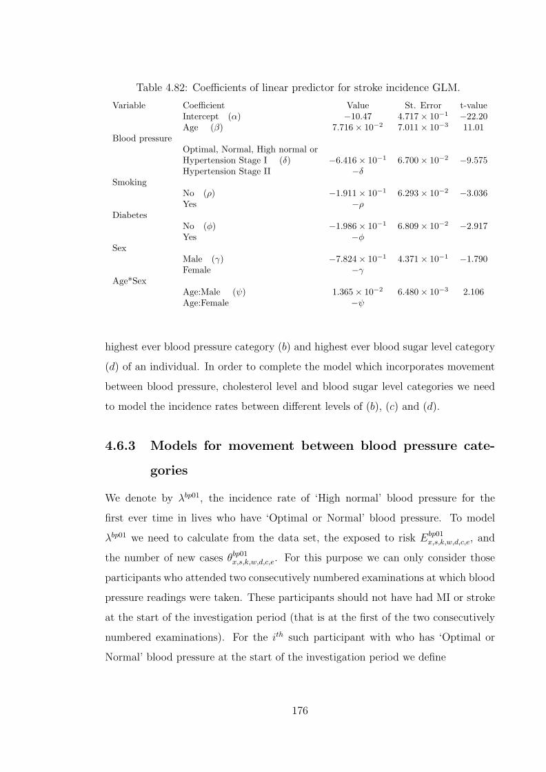
Table 4.82: Coefficients of linear predictor for stroke incidence GLM.
Variable Coefficient Value St. Error t-valueIntercept (α) −10.47 4.717× 10⁻¹ −22.20Age (β) 7.716× 10⁻² 7.011× 10⁻³ 11.01
Blood pressureOptimal, Normal, High normal orHypertension Stage I (δ) −6.416× 10⁻¹ 6.700× 10⁻² −9.575Hypertension Stage II −δ
SmokingNo (ρ) −1.911× 10⁻¹ 6.293× 10⁻² −3.036Yes −ρ
DiabetesNo (φ) −1.986× 10⁻¹ 6.809× 10⁻² −2.917Yes −φ
SexMale (γ) −7.824× 10⁻¹ 4.371× 10⁻¹ −1.790Female −γ
Age*SexAge:Male (ψ) 1.365× 10⁻² 6.480× 10⁻³ 2.106Age:Female −ψ
highest ever blood pressure category (b) and highest ever blood sugar level category
(d) of an individual. In order to complete the model which incorporates movement
between blood pressure, cholesterol level and blood sugar level categories we need
to model the incidence rates between different levels of (b), (c) and (d).
4.6.3 Models for movement between blood pressure cate-
gories
We denote by λbp01, the incidence rate of ‘High normal’ blood pressure for the
first ever time in lives who have ‘Optimal or Normal’ blood pressure. To model
λbp01 we need to calculate from the data set, the exposed to risk Ebp01x,s,k,w,d,c,e, and
the number of new cases θbp01x,s,k,w,d,c,e. For this purpose we can only consider those
participants who attended two consecutively numbered examinations at which blood
pressure readings were taken. These participants should not have had MI or stroke
at the start of the investigation period (that is at the first of the two consecutively
numbered examinations). For the ith such participant with who has ‘Optimal or
Normal’ blood pressure at the start of the investigation period we define
176
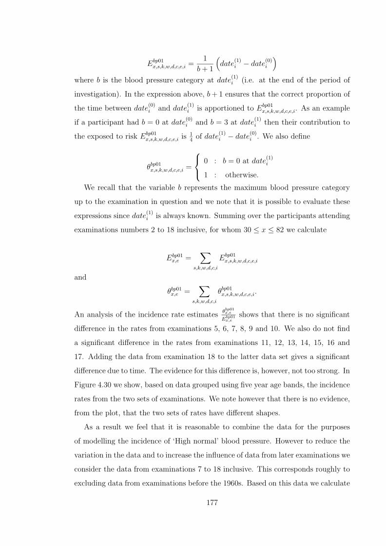
Ebp01x,s,k,w,d,c,e,i =
1
b + 1
(date
(1)i − date
(0)i
)where b is the blood pressure category at date
(1)i (i.e. at the end of the period of
investigation). In the expression above, b + 1 ensures that the correct proportion of
the time between date(0)i and date
(1)i is apportioned to Ebp01
x,s,k,w,d,c,e,i. As an example
if a participant had b = 0 at date(0)i and b = 3 at date
(1)i then their contribution to
the exposed to risk Ebp01x,s,k,w,d,c,e,i is 1
4of date
(1)i − date
(0)i . We also define
θbp01x,s,k,w,d,c,e,i =
0 : b = 0 at date
(1)i
1 : otherwise.
We recall that the variable b represents the maximum blood pressure category
up to the examination in question and we note that it is possible to evaluate these
expressions since date(1)i is always known. Summing over the participants attending
examinations numbers 2 to 18 inclusive, for whom 30 ≤ x ≤ 82 we calculate
Ebp01x,e =
∑s,k,w,d,c,i
Ebp01x,s,k,w,d,c,e,i
and
θbp01x,e =
∑s,k,w,d,c,i
θbp01x,s,k,w,d,c,e,i.
An analysis of the incidence rate estimatesθbp01x,e
Ebp01x,e
shows that there is no significant
difference in the rates from examinations 5, 6, 7, 8, 9 and 10. We also do not find
a significant difference in the rates from examinations 11, 12, 13, 14, 15, 16 and
17. Adding the data from examination 18 to the latter data set gives a significant
difference due to time. The evidence for this difference is, however, not too strong. In
Figure 4.30 we show, based on data grouped using five year age bands, the incidence
rates from the two sets of examinations. We note however that there is no evidence,
from the plot, that the two sets of rates have different shapes.
As a result we feel that it is reasonable to combine the data for the purposes
of modelling the incidence of ‘High normal’ blood pressure. However to reduce the
variation in the data and to increase the influence of data from later examinations we
consider the data from examinations 7 to 18 inclusive. This corresponds roughly to
excluding data from examinations before the 1960s. Based on this data we calculate
177

Age
Inci
denc
e ra
te
30 40 50 60 70 80
0.0
0.05
0.10
0.15
0.20
Exams 5,6,7,8,9,10Exams 11,12,13,14,15,16,17
Figure 4.30: The observed crude incidence rates of ‘High normal’ blood pressure indifferent time periods for females.
Ebp01x,s,k,w,d,c =
∑i,e
Ebp01x,s,k,w,d,c,e,i
and
θbp01x,s,k,w,d,c =
∑i,e
θbp01x,s,k,w,d,c,e,i.
We then assume that
θbp01x,s,k,w,d,c ∼ Poisson
(Ebp01
x,s,k,w,d,c · exp (gx,s,k,w,d,c))
where g(·) is an appropriate linear predictor. On fitting the linear predictor, only
age and BMI are retained as significant. However we did not find a significant
difference in the coefficients of the BMI categories w = 1 and w = 2. Therefore we
calculate
Ebp01x,w∗ =
∑Ebp01
x,s,k,w,d,c
and
θbp01x,w∗ =
∑θbp01
x,s,k,w,d,c
178

where w∗ is obtained from w by combining into one category the two categories
w = 1 and w = 2. This results in 79 data points which we use to fit the linear
predictor assuming
θbp01x,w∗ ∼ Poisson (Ex,w∗ · exp (gx,w∗)) .
This fit achieves a residual deviance of 87 on 76 degrees of freedom and the results
are shown in Table 4.83.
Table 4.83: Coefficients of linear predictor for ‘High normal’ blood pressure incidenceGLM.
Variable Coefficient Value St. Error t-valueIntercept (α) −3.969 3.158× 10⁻¹ −12.57Age (β) 2.199× 10⁻² 5.231× 10⁻³ 4.204
Body mass indexNormal BMI (ν) −9.433× 10⁻² 4.443× 10⁻² −2.123Overweight or Obese −ν
Therefore the incidence of ‘High normal’ blood pressure is modelled by
λbp01x,w = exp (αint + βx + νw)
where the coefficients are given in Table 4.83. The variance-covariance matrix as-
sociated with the parameters in Table 4.83 is given in Table I.132 (see Appendix
I).
The incidence of ‘Hypertension Stage I’ blood pressure for the first ever time in
lives with ‘High Normal’ blood pressure is denoted λbp12. To model λbp12 we calculate
for each participant with ‘High Normal’ blood pressure at date(0)i , the exposed to
risk
Ebp12x,s,k,w,d,c,e,i =
1b
(date
(1)i − date
(0)i
): b = 1, 2 or 3 at date
(1)i
0 : otherwise.
As an example, a participant who remains with ‘High Normal’ blood pressure (b = 1)
up to date(1)i will have exposure for the full
(date
(1)i − date
(0)i
)period. Also the
179

number of cases
θbp12x,s,k,w,d,c,e,i =
1 : b = 2 or 3 at date
(1)i
0 : otherwise.
We calculate Ebp12x,s,k,w,d,c and θbp12
x,s,k,w,d,c based on examinations 7 to 18 inclusive and
assume that
θbp12x,s,k,w,d,c ∼ Poisson
(Ebp12
x,s,k,w,d,c · exp (gx,s,k,w,d,c,))
.
On fitting the linear predictor, g(·), only age and sex are retained as significant
variables. We show in Table 4.84 the coefficients of the fitting based on 79 data
points of Ebp12x,s and θbp12
x,s . This fitting achieved a residual deviance of 66 on 76
degrees of freedom.
Table 4.84: Coefficients of linear predictor for ‘Hypertension Stage I’ blood pressureincidence GLM.
Variable Coefficient Value St. Error t-valueIntercept (α) −3.865 2.718× 10⁻¹ −14.22Age (β) 2.139× 10⁻² 4.331× 10⁻³ 4.938
SexMales (γ) −1.300× 10⁻¹ 3.850× 10⁻² −3.376Females −γ
The incidence of ‘Hypertension Stage I’ blood pressure is modelled by
λbp12x,w = exp (αint + βx + γs)
where the coefficients are given in Table 4.84. The variance-covariance matrices
associated with the parameters in Table 4.84 are also given in Table I.132 (see
Appendix I).
We denote by λbp23 the incidence rate of ‘Hypertension Stage II or Stage III’ for
the first ever time in lives who have ‘Hypertension Stage I’. For the ith participant
with ‘Hypertension Stage I’ at date(0)i , we have
Ebp23x,s,k,w,d,c,e,i =
1b−1
(date
(1)i − date
(0)i
): b = 2 or 3 at date
(1)i
0 : otherwise
180
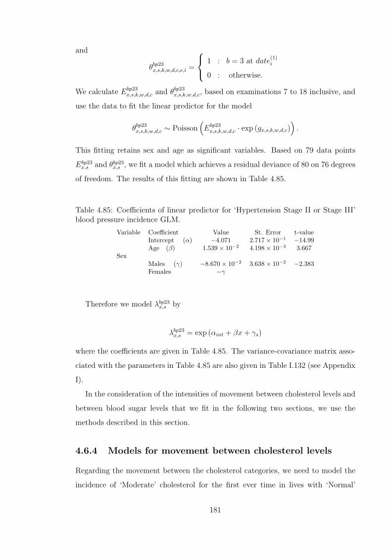
and
θbp23x,s,k,w,d,c,e,i =
1 : b = 3 at date
(1)i
0 : otherwise.
We calculate Ebp23x,s,k,w,d,c and θbp23
x,s,k,w,d,c, based on examinations 7 to 18 inclusive, and
use the data to fit the linear predictor for the model
θbp23x,s,k,w,d,c ∼ Poisson
(Ebp23
x,s,k,w,d,c · exp (gx,s,k,w,d,c))
.
This fitting retains sex and age as significant variables. Based on 79 data points
Ebp23x,s and θbp23
x,s , we fit a model which achieves a residual deviance of 80 on 76 degrees
of freedom. The results of this fitting are shown in Table 4.85.
Table 4.85: Coefficients of linear predictor for ‘Hypertension Stage II or Stage III’blood pressure incidence GLM.
Variable Coefficient Value St. Error t-valueIntercept (α) −4.071 2.717× 10⁻¹ −14.99Age (β) 1.539× 10⁻² 4.198× 10⁻³ 3.667
SexMales (γ) −8.670× 10⁻² 3.638× 10⁻² −2.383Females −γ
Therefore we model λbp23x,s by
λbp23x,s = exp (αint + βx + γs)
where the coefficients are given in Table 4.85. The variance-covariance matrix asso-
ciated with the parameters in Table 4.85 are also given in Table I.132 (see Appendix
I).
In the consideration of the intensities of movement between cholesterol levels and
between blood sugar levels that we fit in the following two sections, we use the
methods described in this section.
4.6.4 Models for movement between cholesterol levels
Regarding the movement between the cholesterol categories, we need to model the
incidence of ‘Moderate’ cholesterol for the first ever time in lives with ‘Normal’
181
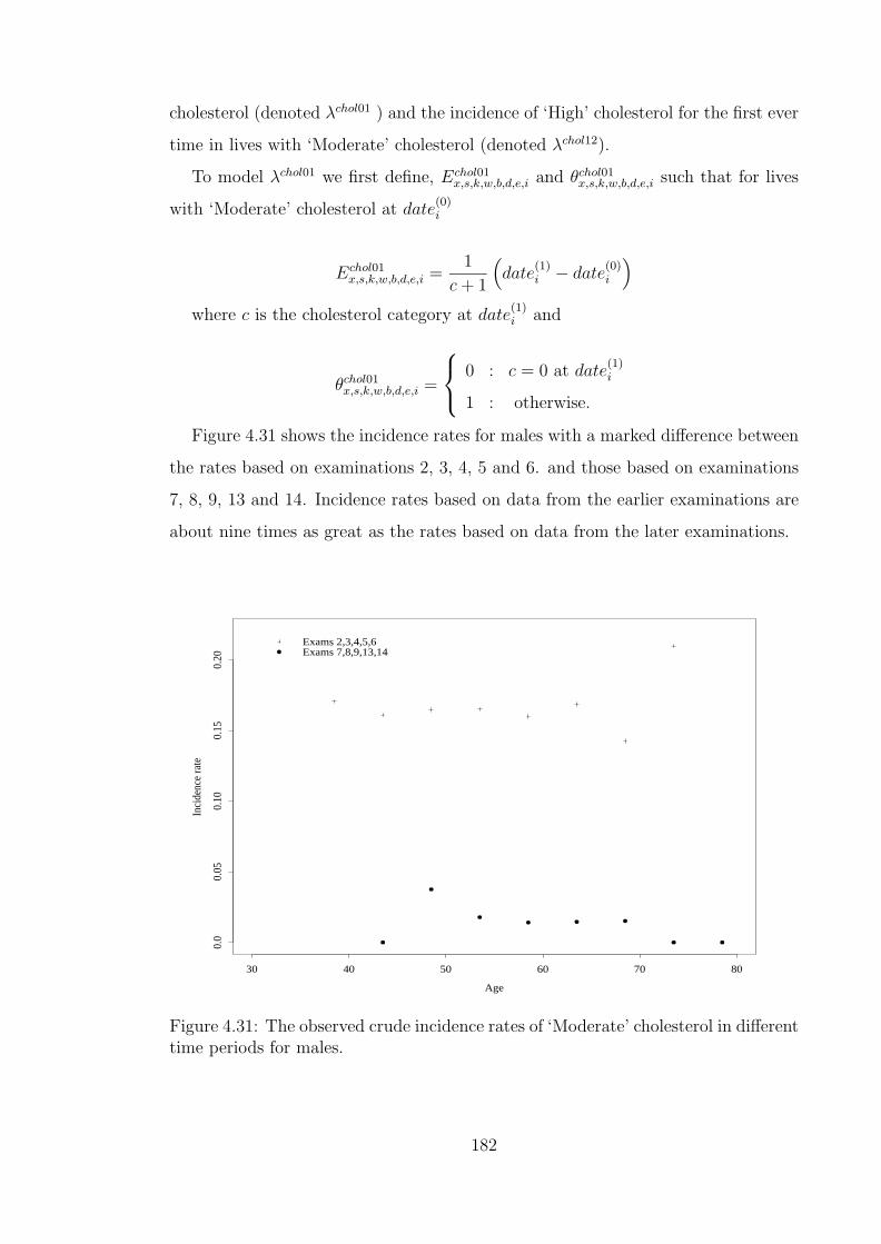
cholesterol (denoted λchol01 ) and the incidence of ‘High’ cholesterol for the first ever
time in lives with ‘Moderate’ cholesterol (denoted λchol12).
To model λchol01 we first define, Echol01x,s,k,w,b,d,e,i and θchol01
x,s,k,w,b,d,e,i such that for lives
with ‘Moderate’ cholesterol at date(0)i
Echol01x,s,k,w,b,d,e,i =
1
c + 1
(date
(1)i − date
(0)i
)where c is the cholesterol category at date
(1)i and
θchol01x,s,k,w,b,d,e,i =
0 : c = 0 at date
(1)i
1 : otherwise.
Figure 4.31 shows the incidence rates for males with a marked difference between
the rates based on examinations 2, 3, 4, 5 and 6. and those based on examinations
7, 8, 9, 13 and 14. Incidence rates based on data from the earlier examinations are
about nine times as great as the rates based on data from the later examinations.
Age
Inci
denc
e ra
te
30 40 50 60 70 80
0.0
0.05
0.10
0.15
0.20
Exams 2,3,4,5,6Exams 7,8,9,13,14
Figure 4.31: The observed crude incidence rates of ‘Moderate’ cholesterol in differenttime periods for males.
182

Therefore to model λchol01 for males we consider Echol01x,s=0,k,w,b,d,e and θchol01
x,s=0,k,w,b,d,e
based on data from examinations 7, 8, 9, 13 and 14. On the assumption that
θchol01x,s=0,k,w,b,d,e ∼ Poisson
(Echol01
x,s=0,k,w,b,d,e · exp (gx,k,w,b,d,e))
we fit the linear predictor g(·) using the data Echol01x,s=0,k,w,b,d,e and θchol01
x,s=0,k,w,b,d,e. The
model retains the time variable e as significant but age and all the other variables
are not retained. For parsimony we intend to derive a model without the variable e
and so we aggregate the data over the 5 examination periods. Using 38 data points
(subdivided by age only), we fit the GLM linear predictor g(·). The fit achieved a
residual deviance of 32 on 37 degrees of freedom and the results are shown in Table
4.86.
Table 4.86: Coefficients of linear predictor for ‘Moderate’ cholesterol incidence GLMfor males.
Variable Coefficient Value St. Error t-valueIntercept −3.312 0.2353 −14.07
Therefore the incidence of ‘Moderate’ cholesterol in males is modelled by
λchol01s=0 = exp(−3.312) = 0.036.
Figure 4.32 shows the incidence rates rates of ‘Moderate’ cholesterol for females
with a difference between those based on the examinations 2, 3, 4, 5, 6 and those
based on examinations 7, 8, 9, 13, 14. The rates from the later examinations are
about half of those from the earlier ones.The two sets of rates have the same general
shape.
To model λchol01 for females we will consider the data from examinations 2, 3,
4, 5 and 6 to determine the shape of the function representing the incidence rates.
We then adjust the level of the function to the level of the rates based on data from
examinations 7, 8, 9, 13, 14. This is due to the fact that there is more data from
examinations 2, 3, 4, 5 and 6 than from examinations 7, 8, 9, 13, 14 which makes
the earlier examinations’ data more reliable in determining the shape of the curve.
However it is our aim to model the level of λchol01 based on more recent rather than
183
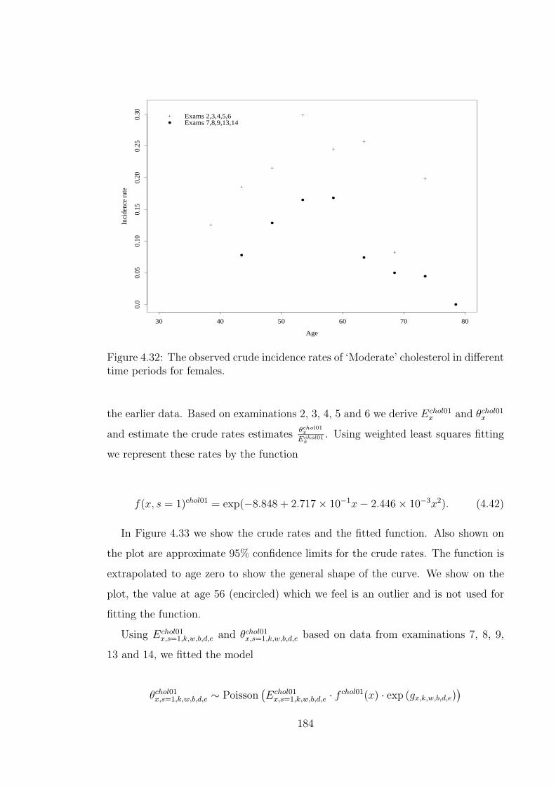
Age
Inci
denc
e ra
te
30 40 50 60 70 80
0.0
0.05
0.10
0.15
0.20
0.25
0.30 Exams 2,3,4,5,6
Exams 7,8,9,13,14
Figure 4.32: The observed crude incidence rates of ‘Moderate’ cholesterol in differenttime periods for females.
the earlier data. Based on examinations 2, 3, 4, 5 and 6 we derive Echol01x and θchol01
x
and estimate the crude rates estimates θchol01x
Echol01x
. Using weighted least squares fitting
we represent these rates by the function
f(x, s = 1)chol01 = exp(−8.848 + 2.717× 10⁻¹x− 2.446× 10−3x2). (4.42)
In Figure 4.33 we show the crude rates and the fitted function. Also shown on
the plot are approximate 95% confidence limits for the crude rates. The function is
extrapolated to age zero to show the general shape of the curve. We show on the
plot, the value at age 56 (encircled) which we feel is an outlier and is not used for
fitting the function.
Using Echol01x,s=1,k,w,b,d,e and θchol01
x,s=1,k,w,b,d,e based on data from examinations 7, 8, 9,
13 and 14, we fitted the model
θchol01x,s=1,k,w,b,d,e ∼ Poisson
(Echol01
x,s=1,k,w,b,d,e · f chol01(x) · exp (gx,k,w,b,d,e))
184

Age
Off
set v
alue
0 20 40 60 80
0.0
0.1
0.2
0.3
0.4
0.5
0.6
Figure 4.33: The observed and fitted chol01 offset incidence rates for females.
where g(·) is a linear predictor and f chol01(x) is an offset function given by Equation
(4.42). None of the variables of the linear predictor was retained as significant.
Therefore based on 35 data points (subdivided by age only) the GLM fit for the
linear predictor achieved a residual deviance of 34 on 34 degrees of freedom. The
results are shown in Table 4.87.
Table 4.87: Coefficients of linear predictor for ‘Moderate’ cholesterol incidence GLMfor females.
Variable Coefficient Value St. Error t-valueIntercept −0.6446 0.126 −5.117
Therefore the incidence of ‘Moderate’ cholesterol in females is modelled by
λchol01x,s=1 = exp(−9.493 + 2.717× 10⁻¹x− 2.446× 10−3x2).
185
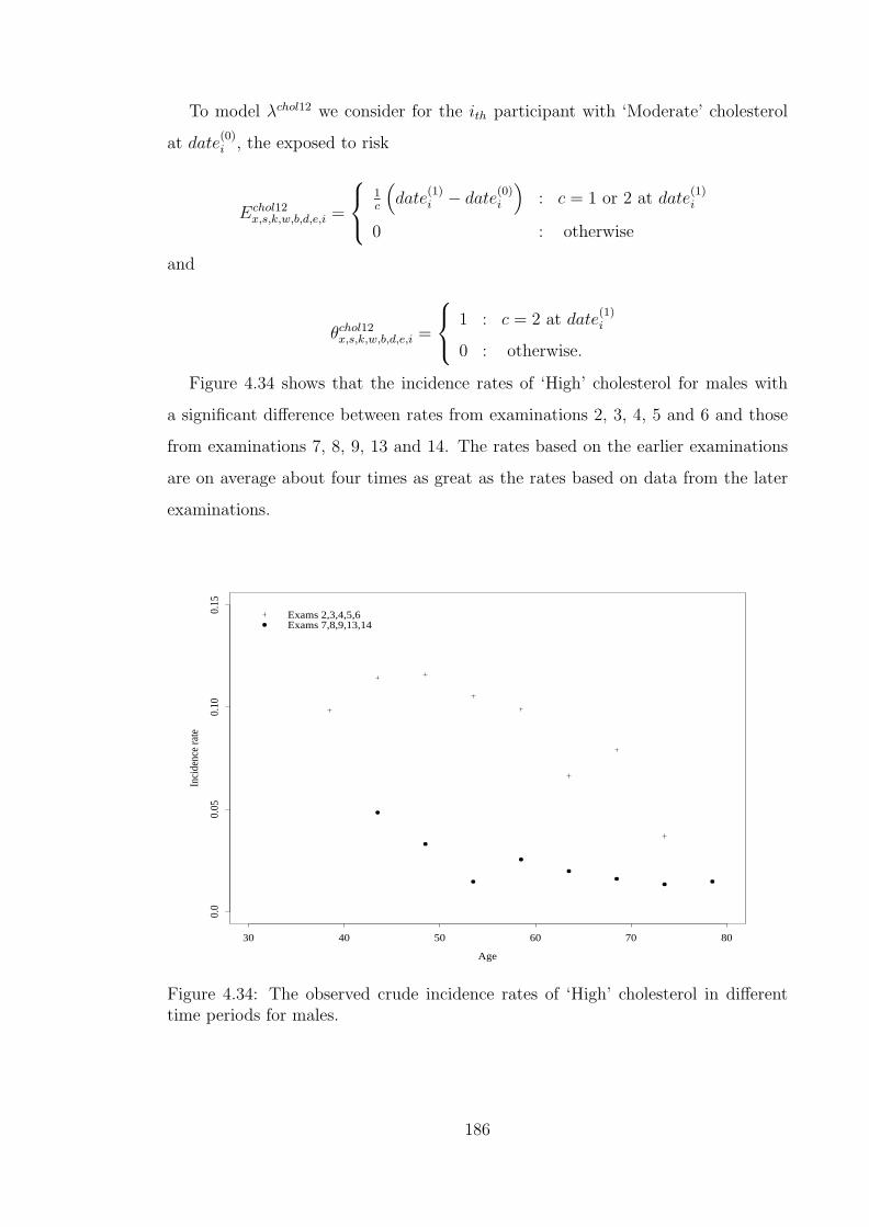
To model λchol12 we consider for the ith participant with ‘Moderate’ cholesterol
at date(0)i , the exposed to risk
Echol12x,s,k,w,b,d,e,i =
1c
(date
(1)i − date
(0)i
): c = 1 or 2 at date
(1)i
0 : otherwise
and
θchol12x,s,k,w,b,d,e,i =
1 : c = 2 at date
(1)i
0 : otherwise.
Figure 4.34 shows that the incidence rates of ‘High’ cholesterol for males with
a significant difference between rates from examinations 2, 3, 4, 5 and 6 and those
from examinations 7, 8, 9, 13 and 14. The rates based on the earlier examinations
are on average about four times as great as the rates based on data from the later
examinations.
Age
Inci
denc
e ra
te
30 40 50 60 70 80
0.0
0.05
0.10
0.15
Exams 2,3,4,5,6Exams 7,8,9,13,14
Figure 4.34: The observed crude incidence rates of ‘High’ cholesterol in differenttime periods for males.
186

We use the data from examinations 2, 3, 4, 5 and 6 to determine the shape of
the incidence curve and then adjust it to the level of the rates derived from the
data for examinations 7, 8, 9, 13 and 14. Using single years of age, we calculate the
incidence rates estimates based on data from the earlier set of examinations,θx,s=0
Ex,s=0.
Using weighted least squares, we fit the function
f(x, s = 0)chol12 = exp(−5.533 + 1.432× 10⁻¹x− 1.539× 10−3x2) (4.43)
to these crude rates. Figure 4.35 shows the crude rates and the fitted function. We
also show the approximate 95% confidence limits for the crude rates. The function
is extrapolated beyond the fitted ages to show the general shape of the curve.
Age
Offs
et v
alue
0 20 40 60 80
0.0
0.05
0.10
0.15
0.20
0.25
0.30
Figure 4.35: The observed and fitted chol12 offset incidence rates for males.
We then calculate, from the data based on examinations 7, 8, 9, 13 and 14,
Echol12x,s=0,k,w,b,d,e and θchol12
x,s=0,k,w,b,d,e. We assume that
θchol12x,s=0,k,w,b,d,e ∼ Poisson
(Echol12
x,s=0,k,w,b,d,e · f(x, s = 0)chol12 · exp (gx,k,w,b,d,e))
187
where f(x, s = 0)chol12 is the offset function in Equation (4.43) and g(·) is an ap-
propriate linear predictor. The fit retains the time variable e as significant but the
other variables are not retained. However, for parsimony we group the data over all
the examinations 7, 8, 9, 13 and 14. Based on 40 data points (subdivided by age
only) the fitting achieves a residual deviance of 51 on 39 degrees of freedom. The
results are shown in Table 4.88.
Table 4.88: Coefficients of linear predictor for ‘High’ cholesterol incidence GLM formales.
Variable Coefficient Value St. Error t-valueIntercept −1.324 0.1259 −10.52
Therefore the incidence of ‘High’ cholesterol in males is modelled by
λchol12x,s=0 = exp(−6.857 + 1.432× 10⁻¹x− 1.539× 10−3x2).
We note that from the results shown in Table 4.88 the variation in the fitted rates
relative to the mean, is more than we would expect for a Poisson model. We feel
this is due to the effect of grouping over the examinations 7, 8, 9, 13 and 14. This
problem does not arise if we group the data over the examinations 8, 9, 13 and 14
only. However there is significantly less data from examinations 8, 9, 13 and 14.
Therefore we will use the model based on examinations 7, 8, 9, 13 and 14 and this
can be further refined if better data becomes available.
Figure 4.36 shows a comparison of the incidence rates between those based on
the data from examinations 2, 3, 4, 5, and 6 and those from the later examinations,
for females. The difference between the two sets of rates is noticeable but the plot
also shows that the rates have the same general shape. Incidence rates based on
data from the earlier examinations are on average about three times as great as the
rates based on data from the later examinations.
To model the incidence of ‘High’ cholesterol in females we use the data from
examinations 2, 3, 4, 5, and 6 to determine the shape of the incidence curve and
then adjust the level to that of the rates based on the later examinations. Using
single years of age, we derive, from the earlier examinations, the estimates of the
188

Age
Inci
denc
e ra
te
30 40 50 60 70 80
0.0
0.05
0.10
0.15
0.20
Exams 2,3,4,5,6Exams 7,8,9,13,14
Figure 4.36: The observed crude incidence rates of ‘High’ cholesterol in differenttime periods for females.
incidence rates for ‘High’ cholesterol, θchol12x
Echol12x
. Using weighted least squares, we fit
the function
f(x, s = 1)chol12 = exp(−14.31 + 4.744× 10⁻¹x− 4.470× 10−3x2) (4.44)
to the crude rates. Figure 4.37 shows the crude rates and the fitted function. We
also show the approximate 95% confidence limits for the crude rates and the function
is extrapolated beyond the fitted ages to show the general shape of the curve.
Using data from examinations 7, 8, 9, 13 and 14, we fitted the model
θchol12x,s=1,k,w,b,d,e ∼ Poisson
(Echol12
x,s=1,k,w,b,d,e · f(x, s = 1)chol12 · exp (gx,k,w,b,d,e))
where f(x, s = 1)chol12 is the offset function in Equation (4.44) and g(·) is an appro-
priate linear predictor. None of the variables in the linear predictor was retained as
189

Age
Offs
et v
alue
0 20 40 60 80
0.0
0.1
0.2
0.3
Figure 4.37: The observed and fitted chol12 offset incidence rates for females.
significant. In Table 4.89 we show the results of the fitting, based on 40 data points,
which achieves a residual deviance of 33 on 39 degrees of freedom.
Table 4.89: Coefficients of linear predictor for ‘High’ cholesterol incidence GLM forfemales.
Variable Coefficient Value St. Error t-valueIntercept −0.9638 7.596× 10⁻² −12.12
Therefore the incidence of ‘High’ cholesterol in females is modelled by
λchol12x,s=1 = exp(−15.27 + 4.744× 10⁻¹x− 4.470× 10−3x2).
4.6.5 Models for movement between blood sugar levels
We denote the incidence of diabetes by λdiab. From the data we consider the exposed
to risk Ediab and the number of new cases θdiab. For the ith participant with bsl < 126
at date(0), we define
190

Ediabx,s,k,w,b,c,e,i =
1
d + 1
(date
(1)i − date
(0)i
)where d is the blood sugar level category at date
(1)i and
θdiabx,s,k,w,b,c,e,i =
0 : d = 0 at date
(1)i
1 : otherwise.
We can derive the data Ediabx and θdiab
x by aggregating details over examinations 2,
3, 8, 9, 12, 13, 14, 15, 16, 17 and 18. However we note that examinations 2 and
3 are removed in time from the rest of the data. We therefore only consider data
from the remaining examinations. An analysis of the incidence rates for various
examination periods show that for examinations 8, 9, 12, 13, 14 and 15, there
is no significant difference in the incidence rates θdiabx
Ediabx
due to time. However the
rates from examinations 16, 17 and 18 show some differences from rates from earlier
examinations and also significant variation within themselves. Figure 4.38 shows the
crude incidence rates grouped using five-year age bands for the two time periods.
Age
Inci
denc
e ra
te
40 50 60 70 80
0.0
0.01
0.02
0.03
0.04
0.05
Exams 8,9,12,13,14,15Exams 16,17,18
Figure 4.38: The observed crude incidence rates of diabetes in different time periods.
191

There is less data for the older ages and no data at the younger ages in the later
examinations’ data. However we also need to capture the recent levels represented
by the later data. Consequently, to model the diabetes incidence we aggregate the
data over the examinations 8, 9, 12, 13, 14, 15, 16, 17 and 18 and use it to fit a
GLM.
We therefore calculate Ediabx,s,k,w,b,c and θdiab
x,s,k,w,b,c and assume that
θdiabx,s,k,w,b,c ∼ Poisson
(Ediab
x,s,k,w,b,cexp (gx,s,k,w,b,c)),
where g(·) is a linear predictor. On fitting the linear predictor only age and BMI
are retained as significant variables. However we found no significant difference in
the coefficients of the BMI categories w = 0 and w = 1 (‘Normal’ and ‘Overweight’
categories). We derive a reduced data set Ediabx,w∗ and θdiab
x,w∗ where w∗ is obtained from
w by combining the two categories w = 0 and w = 1 into one. The results shown in
Table 4.90 represent the fitting based on 77 data points which achieved a residual
deviance of 88 on 74 degrees of freedom.
Table 4.90: Coefficients of linear predictor for diabetes incidence GLM.
Variable Coefficient Value St. Error t-valueIntercept (α) −6.703 3.294× 10⁻¹ −20.35Age (β) 4.448× 10⁻² 4.874× 10⁻³ 9.126
Body Mass IndexNormal or Overweight (ν) −2.434× 10⁻¹ 4.332× 10⁻² −5.619Obese −ν
Therefore the model for diabetes incidence is
λdiabx,w = exp (αint + βx + νw∗)
where the coefficients are given in Table 4.90. The variance-covariance matrix as-
sociated with the parameters in Table 4.90 is given in Table I.132 (see Appendix
I).
Table 4.91 shows a summary of the factors relevant to the various models we have
derived.
We will apply these models for MI, stroke and the risk factors in a CI insurance
model in Chapter 5. Now we assess the reasonableness of the models for the risk
192

Table 4.91: Summary of models.
Function Offset Age Sex Smoking BMI Blood Pressure Cholesterol DiabetesλMI • • • • • •λstroke • • • • •
λbp01 • •λbp12 • •λbp23 • •
λchol01males
λchol01females Exponential •
λchol12males Exponential •
λchol12females Exponential •
λdiab • •
factors and the adequacy of the MI and stroke models by comparing them to other
published results.
4.7 Discussion of risk factor models
4.7.1 Blood pressure
There is a fundamental difficulty in comparing the blood pressure models we have
developed with other results. This is due to the fact we divide the blood pressure
continuum into 4 categories (a multiple threshold model, MTM) while the other
studies available to us divide the same continuum into two categories (single thresh-
old models, STM). We therefore need some way in which to compare the two results.
We will perform two comparisons.
The first comparison considers the rates of hypertension based on a STM applied
to the Framingham data alongside the hypertension rates based on the data from
The Morbidity Statistics from General Practice (M.S.G.P.) fourth national study
(McCormick et al. (1995)). For the M.S.G.P. data we define Hypertension as diag-
noses categorised under ICD codes 410, 411, and 419 in the study. Only first ever
cases are considered for this analysis. We assume that for this survey the diagnosis
193

definition of ‘hypertension’, conforms to nationally agreed guidelines. Guidelines is-
sued in 1989 (Swales et al. (1989)) suggested treatment for lives with dbp at 100 mm
Hg or higher and updated guidelines issued in 1999 (Ramsay et al. (1999)) suggest
starting treatment for hypertension in lives with sbp greater than 160 mm Hg or
dbp greater than 100 mm Hg. The actual clinical decision to initiate treatment will
consider other factors like the presence or absence of organ damage, alongside the
recommended levels of sbp and dbp.
For each age x, we derive from (McCormick et al. (1995)), the number of new
hypertension cases θMSGPx . We can also derive the amount of time spent in the study
by lives aged x, which we denote EMSGPx . To calculate this we use the convention
that a life who develops hypertension during the study contributes half of the time
they spend in the study to the value of EMSGPx . Lives who did not develop hyper-
tension contribute time equivalent to the full time they spent in the study. The
problem with the estimate EMSGPx is that it includes time contributed by some lives
who have already had hypertension. Using the data in the study, lives who have had
hypertension can not be distinguished from the lives who have never had hyperten-
sion. Therefore we need to determine the appropriate amount by which to reduce
EMSGPx using other sources of information. We use the data on the prevalence of
hypertension in the population in England to do that.
Table 4.92 shows the prevalence of hypertension in England according to the
Health Survey for England 1998 (Erens and Primatesta (1999)). These values are
based on hypertension defined as systolic blood pressure exceeding 160 mm Hg or
diastolic blood pressure exceeding 95 mm Hg.
Table 4.92: Prevalence of hypertension based on the 1998 Health Survey for England.(Source: Erens and Primatesta (1999).)
Age group16-24 25-34 35-44 45-54 55-64 65-74 75+
Males 0.013 0.018 0.076 0.174 0.324 0.426 0.449Females 0.004 0.013 0.042 0.137 0.273 0.486 0.552
194

Using these data and assuming a maximum possible age of 100 we fitted the
models
λbp prev malesx = 30.21
[0.122510.77exp (−0.1225x) x9.77
Γ(10.77)
](4.45)
and
λbp prev femalesx = 31.88
[0.167014.75exp (−0.1670x) x13.75
Γ(14.75)
](4.46)
to represent the prevalence of hypertension in males and females, respectively. We
use formulae (4.45) and (4.46) to adjust the individual contributions to EMSGPx ,
EMSGPx,i , by using
(1− λbp prev males
x
)EMSGP
x,i or(1− λbp prev females
x
)EMSGP
x,i as ap-
propriate. We use the adjusted data to estimate the incidence of hypertension
θMSGPx
EMSGPx
and approximate variance of the estimates θMSGPx
(EMSGPx )2.
From the Framingham data, using the methods of Section 4.6.3, we derive the
number of new ‘Hypertension Stages II and III’ for the first time ever in lives who are
in the ‘Optimal or Normal’, ‘High Normal’ or ‘Hypertension Stage I’ categories. We
denote this θFraminghamx and we derive the exposed to risk corresponding to it which
we denote EFraminghamx . These values are based on details from examinations 7 to
18 inclusive only. We can then estimate the incidence of hypertension (defined as
systolic blood pressure exceeding 160 mm Hg or diastolic blood pressure exceeding
100 mm Hg), θFraminghamx
EFraminghamx
.
Figure 4.39 shows the comparison of the hypertension incidence rates estimates
from the Framingham data and from the M.S.G.P. (McCormick et al. (1995)), for
males and females combined. The Framingham rates are higher than the M.S.G.P.
rates. This is consistent with an expectation of lowering incidence rates given the
difference in times between the two studies. To achieve a good fit of the hypertension
incidence in the M.S.G.P. study, a model based on the Framingham data may need
to be adjusted slightly to lower the rates. We feel that any such adjustment has to
be minor and may not have a significant effect in a model with other factors, like
the CI insurance model we develop in Chapter 5.
Our second assessment of the blood pressure models developed in section 4.6.3
considers the prevalence rates based on the 1998 Health Survey for England which
we have represented by formulae (4.45) and (4.46). Based on our MTM we calcu-
late the implied prevalence of hypertension in the population and compare it with
195

Age
Inci
denc
e ra
te
50 60 70 80
0.0
0.02
0.04
0.06
FraminghamM.S.G.P.
Figure 4.39: Comparison of hypertension incidence rates from the Framingham dataand the M.S.G.P. data.
that modelled by formulae (4.45) and (4.46). We do this using a five state model
incorporating the four blood pressure categories and death. This is shown in Figure
4.40.
We assume that in Figure 4.40, a life is in State 0 at age 0. The movement
into the various blood pressure categories is given by the models in Section 4.6.3 as
labelled. We assume the mortality is given by ELT15M and ELT15F without any
adjustments. We calculate the probability of being in any of the five states at any age
for lives having started in State 0 at age 0. We note that since the models depend
on age, sex and BMI we have three models like Figure 4.40 representing BMI
categories for each sex. We calculate for each age, the prevalence of hypertension
as the probability of being in State 3 given that they are still alive. For each sex
we can calculate the age specific weighted average of the prevalence over the BMI
categories. To achieve this we assume that the population has fixed proportions in
the various BMI categories and those are as given by the 1998 Health Survey for
196

-
HHHHHHHHHHHHj
State 0b = 0
λbp01x+r,w
λDx+r,s
-
?
State 1b = 1
λbp12x+r,s
λDx+r,s
-
?
State 2b = 2
λbp23x+r,s
λDx+r,s
©©©©©©©©©©©©¼
State 3b = 3
λDx+r,s
State 4Dead
Figure 4.40: Model for movement between blood pressure categories.
England (Erens and Primatesta (1999)), as represented in Table 4.93.
Table 4.93: Subdivision (proportions) of population in England by BMI category.(Source: Erens and Primatesta (1999).)
Males FemalesBMI ≤ 25 0.37 0.4725 < BMI ≤ 30 0.46 0.32BMI > 30 0.17 0.21
In Figure 4.41 we show the prevalence of hypertension from our model as derived
by the above calculation together with the prevalence represented by formulae (4.45)
and (4.46). Our models produce prevalence rates which are very close to those in
the population of England as given by the survey of 1998.
4.7.2 Cholesterol
As was the case for the assessment of blood pressure models, the three categories that
we use for cholesterol classification make comparisons with other studies difficult.
Comparisons with the models we have developed for cholesterol can only be reliably
done with studies in which actual cholesterol readings were taken. This is due
to the fact that, unlike blood pressure and blood sugar level, movement across
cholesterol categories is unlikely to give immediate or noticeable symptoms that
can be used as a proxy for blood cholesterol level changes. The only such study we
had access to is the Health Survey for England (Erens and Primatesta (1999)) which
reported the prevalence of hypercholesterolaemia. Table 4.94 shows these prevalence
197

Females
Age
Hyp
erte
nsio
n pr
eval
ence
30 40 50 60 70 80
0.0
0.2
0.4
0.6
Our modelH.S.E. 1998 rates
Males
Age
Hyp
erte
nsio
n pr
eval
ence
30 40 50 60 70 800.
00.
20.
40.
6
Our modelH.S.E. 1998 rates
Figure 4.41: Comparison of hypertension prevalence rates from our bp models withthe Health Survey for England 1998 rates.
rates for the 1998 survey and also for the 1994 survey and we note that Erens and
Primatesta (1999) define hypercholesterolaemia as having total cholesterol exceeding
about 251mg/dL.
Table 4.94: Prevalence of hypercholesterolaemia based on the Health Survey forEngland. (Source: Erens and Primatesta (1999).)
Age group16–24 25–34 35–44 45–54 55–64 65–74 75+ All ages
Males (1998) 0.019 0.108 0.169 0.238 0.229 0.264 0.202 0.18Females (1998) 0.029 0.067 0.088 0.22 0.374 0.480 0.444 0.224
Males (1994) 0.036 0.147 0.309 0.393 0.407 0.383 0.301 0.279Females (1994) 0.048 0.098 0.134 0.322 0.574 0.674 0.576 0.319
We represent the 1998 prevalence rates with the functions:
λchol prev malesx = 20.5
[0.06495.13exp (−0.0649x) x4.13
Γ(5.13)
](4.47)
198

-
@@
@@
@@R
State 0c = 0
λchol01x+r,s
λDx+r,s
-
?
State 1c = 1
λchol12x+r,s
λDx+r,s
¡¡
¡¡
¡¡ª
State 2c = 2
λDx+r,s
State 3Dead
Figure 4.42: Model for movement between cholesterol categories.
and
λchol prev femalesx = 0.0401 + 25.4
[0.15913.0exp (−0.159x) x12.0
Γ(13.0)
]. (4.48)
To estimate the prevalence of hypercholesterolaemia consistent with the models de-
veloped in Section 4.6.4 we construct a four state stochastic model where the three
cholesterol categories and death comprise the states. The transition intensities be-
tween the cholesterol category states are given by the cholesterol models we devel-
oped in Section 4.6.4 and the mortality is given by ELT15F and ELT15M without
adjustments. This model is shown in Figure 4.42.
If we assume that all lives are in State 0 at age 0 we can estimate the prevalence
at any future age as the probability of being in State 2 given that the life is not
dead.
In Figure 4.43 we show the prevalence of hypercholesterolaemia from our model
as derived by the above calculation together with the prevalence represented by
formulae (4.47) and (4.48).
The difference in the prevalence rates shown in Figure 4.43 is consistent with an
expected fall in the incidence of hypercholesterolaemia in the time period between
the Framingham study and 1998. We note that the values shown in Table 4.94
show that even in just the four years between 1994 and 1998 the prevalence of
hypercholesterolaemia fell from 28% to 18% for males and from 32% to 22% for
females. However we do not expect the prevalence of hypercholesterolaemia to be
higher in our model than in the Health Survey for England rates as it is for females
at the younger ages. We feel that this is due to our models underestimating the
199

Females
Age
Hyp
erch
oles
tero
laem
ia p
reva
lenc
e
30 40 50 60 70 80
0.0
0.2
0.4
0.6
0.8
Our modelH.S.E. 1998 rates
Males
AgeH
yper
chol
este
rola
emia
pre
vale
nce
30 40 50 60 70 80
0.0
0.1
0.2
0.3
0.4
0.5
0.6
Our modelH.S.E. 1998 rates
Figure 4.43: Comparison of hypercholesterolaemia prevalence rates from our cholmodels with the Health Survey for England 1998 rates.
transition intensities between cholesterol categories at these ages. However we would
need more data at the younger ages to refine the models. Consequently we will use
the models developed in Section 4.6.4 for the applications in Chapter 5.
4.7.3 Diabetes
We compare the rates of diabetes incidence based on the Framingham data with
the diabetes incidence rates from the M.S.G.P. (McCormick et al. (1995)). Only
first ever cases of diabetes are considered for this analysis. We assume that for
this survey the diagnosis definition of ‘diabetes’ conforms to professional medical
guidelines. The World Health Organisation (1985) defined diabetes as a fasting
plasma glucose level exceeding 140 mg/dL.
For each age x, we derive from McCormick et al. (1995) the number of new
diabetes cases θMSGPx . We follow the methods used in Section 4.7.1 to estimate the
amount of time spent in the study by lives aged x, which we denote EMSGPx . To
adjust EMSGPx for lives who already have diabetes we need the prevalence of diabetes
200
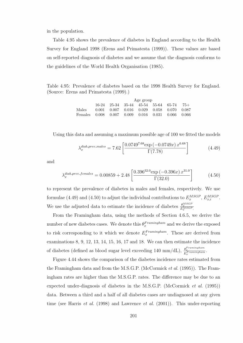
in the population.
Table 4.95 shows the prevalence of diabetes in England according to the Health
Survey for England 1998 (Erens and Primatesta (1999)). These values are based
on self-reported diagnosis of diabetes and we assume that the diagnosis conforms to
the guidelines of the World Health Organisation (1985).
Table 4.95: Prevalence of diabetes based on the 1998 Health Survey for England.(Source: Erens and Primatesta (1999).)
Age group16-24 25-34 35-44 45-54 55-64 65-74 75+
Males 0.001 0.007 0.016 0.029 0.058 0.070 0.087Females 0.008 0.007 0.009 0.016 0.031 0.066 0.066
Using this data and assuming a maximum possible age of 100 we fitted the models
λdiab prev malesx = 7.62
[0.07497.68exp (−0.0749x) x6.68
Γ(7.78)
](4.49)
and
λdiab prev femalesx = 0.00859 + 2.48
[0.39632.0exp (−0.396x) x31.0
Γ(32.0)
](4.50)
to represent the prevalence of diabetes in males and females, respectively. We use
formulae (4.49) and (4.50) to adjust the individual contributions to EMSGPx , EMSGP
x,i .
We use the adjusted data to estimate the incidence of diabetes θMSGPx
EMSGPx .
From the Framingham data, using the methods of Section 4.6.5, we derive the
number of new diabetes cases. We denote this θFraminghamx and we derive the exposed
to risk corresponding to it which we denote EFraminghamx . These are derived from
examinations 8, 9, 12, 13, 14, 15, 16, 17 and 18. We can then estimate the incidence
of diabetes (defined as blood sugar level exceeding 140 mm/dL), θFraminghamx
EFraminghamx
.
Figure 4.44 shows the comparison of the diabetes incidence rates estimated from
the Framingham data and from the M.S.G.P. (McCormick et al. (1995)). The Fram-
ingham rates are higher than the M.S.G.P. rates. The difference may be due to an
expected under-diagnosis of diabetes in the M.S.G.P. (McCormick et al. (1995))
data. Between a third and a half of all diabetes cases are undiagnosed at any given
time (see Harris et al. (1998) and Lawrence et al. (2001)). This under-reporting
201

is also expected to explain the shape of the incidence curve for the M.S.G.P. (Mc-
Cormick et al. (1995)) data, which falls at the older ages. Less likely, having higher
Framingham rates than M.S.G.P. rates may be consistent with a lowering of diabetes
incidence rates (given the fixed diagnosis threshold) due to the difference in time
between the two studies. Our conclusion is that the incidence rates represented by
the two data sets are not similar. However we note that:
(a) Our expectation of under-diagnosis in the M.S.G.P. (McCormick et al. (1995)
and Erens and Primatesta (1999)) means that if the correct incidence of diagno-
sis were reported, it may well be similar to that modelled from the Framingham
data.
(b) If we use the diabetes incidence modelled from the Framingham data in a model
to estimate MI or stroke incidence, as we will do in Chapter 5, the MI or stroke
incidence that we get is consistent with that of Dinani et al. (2000).
For the above reasons we will use the diabetes model of Section 4.6.5 for the CI
model in Chapter 5.
4.8 Assessment of CHD and stroke model ade-
quacy
In the analyses below we use the occupancy probabilities associated with states
in the ‘CHD and stroke’ model. This requires the parameterisation of the mor-
tality transitions into the ‘Dead’ state. The mortality, λDx+t,s, is that of ELT15M
and ELT15F (λELT15x,s ) adjusted for deaths due to MI and stroke. The mortality
adjustments are such that
λDx+t,s = (1− φCHD
x,s − φstrokex,s )× λELT15
x,s
and the adjustment factors φCHDx,s and φstroke
x,s , which are sex specific, are discussed
in Appendix G.
202
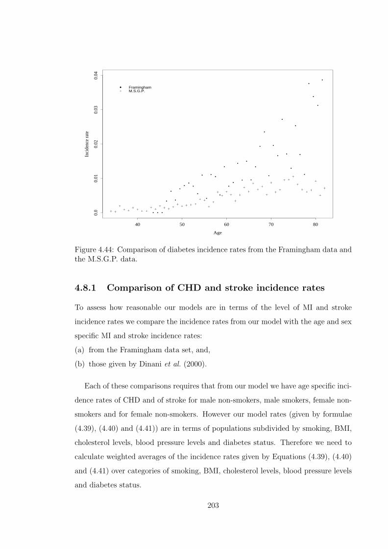
Age
Inci
denc
e ra
te
40 50 60 70 80
0.0
0.01
0.02
0.03
0.04
FraminghamM.S.G.P.
Figure 4.44: Comparison of diabetes incidence rates from the Framingham data andthe M.S.G.P. data.
4.8.1 Comparison of CHD and stroke incidence rates
To assess how reasonable our models are in terms of the level of MI and stroke
incidence rates we compare the incidence rates from our model with the age and sex
specific MI and stroke incidence rates:
(a) from the Framingham data set, and,
(b) those given by Dinani et al. (2000).
Each of these comparisons requires that from our model we have age specific inci-
dence rates of CHD and of stroke for male non-smokers, male smokers, female non-
smokers and for female non-smokers. However our model rates (given by formulae
(4.39), (4.40) and (4.41)) are in terms of populations subdivided by smoking, BMI,
cholesterol levels, blood pressure levels and diabetes status. Therefore we need to
calculate weighted averages of the incidence rates given by Equations (4.39), (4.40)
and (4.41) over categories of smoking, BMI, cholesterol levels, blood pressure levels
and diabetes status.
203

The weights to use for BMI and smoking status in the calculation of the weighted
averages are derived from the distribution of the England and Wales population
by BMI and smoking status (see Tables 4.93 and 4.96). The BMI and smoking
distributions are assumed to be independent of each other such that the proportion of
the male population in the, say, non-smokers and BMI ≤ 25 category subpopulation
is 0.37× 0.72 = 0.2664.
Table 4.96: Subdivision (proportions) of population in England by smoking status.(Source: Erens and Primatesta (1999).)
Males FemalesSmokers 0.28 0.27Non-smokers 0.72 0.73
The weights to use for the cholesterol levels, blood pressure levels and diabetes
status categories are derived from the occupancy probabilities of the associated
‘CHD and stroke’ model. We calculate the probability of being in any state of
the model, conditional on the state not being one of the three absorbing states.
It is assumed that all lives are in the chol0, bp0 state at age 30 and movement
through the model is determined by the models we developed earlier in this chapter.
These occupancy probabilities are calculated using the iterative method described
in Waters and Wilkie (1987).
In Figure 4.45 we show the age and sex specific weighted averages of the MI and
stroke incidence rates from our model together with the observed crude incidence
rates from the Framingham data. The plot shows a good fit to the Framingham rates
in all cases. The fit for CHD (Males) is slightly lower than the Framingham rates
mainly due to the fact that for our model we use cholesterol incidence rates from the
later examinations which are much lower than the average rates. The Framingham
crude rates shown in the graphs are based on data covering examinations 2 to 16
inclusive.
In Figure 4.46 we show the comparison of the rates from our model with those
from England as given by Dinani et al. (2000). The plots also show a good fit to
the Dinani et al. (2000) rates. This is particularly so when we consider ages below
204

CHD (Males)
Age
Inci
denc
e ra
te
30 40 50 60 70 80
0.0
0.02
0.04
Our model
Framingham crude rates
CHD (Females)
Age
Inci
denc
e ra
te
30 40 50 60 70 80
0.0
0.00
50.
010
0.01
5 Our modelFramingham crude rates
Stroke (Males)
Age
Inci
denc
e ra
te
30 40 50 60 70 80
0.0
0.01
00.
020 Our model
Framingham crude rates
Stroke (Females)
Age
Inci
denc
e ra
te
30 40 50 60 70 800.
00.
005
0.01
5
Our model
Framingham crude rates
Figure 4.45: Comparison of incidence rates from our model and those from theFramingham data.
60. The closeness of the two sets of rates is a very reassuring feature given that:
(a) many assumptions are made in our model,
(b) we construct and parameterise a large number of sub-models that make up the
input to our model and
(c) some of the data sets and results used for the parameterisation of our models
come from a time period very removed from the late 1990’s to which the Dinani
et al. (2000) rates relate.
4.8.2 Comparison of CHD and stroke probability rates
The two comparisons done above compare the model output with other rates that
would be considered as instantaneous incidence rates. We also need to assess the
model for adequacy in estimating probabilities of events over a longer period of time.
We need to consider the probabilities of being in the CHD or stroke state ( state
23 or 24) given a starting state, a starting age and the time period. To assess these
205
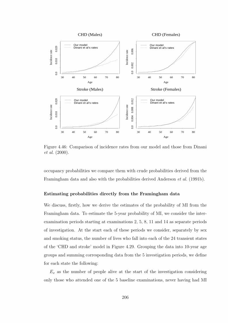
CHD (Males)
Age
Inci
denc
e ra
te
30 40 50 60 70 80
0.0
0.01
00.
020 Our model
Dinani et al’s rates
CHD (Females)
Age
Inci
denc
e ra
te
30 40 50 60 70 80
0.0
0.00
20.
006
Our modelDinani et al’s rates
Stroke (Males)
Age
Inci
denc
e ra
te
30 40 50 60 70 80
0.0
0.01
00.
020 Our model
Dinani et al’s rates
Stroke (Females)
Age
Inci
denc
e ra
te
30 40 50 60 70 800.
00.
004
0.00
80.
012 Our model
Dinani et al’s rates
Figure 4.46: Comparison of incidence rates from our model and those from Dinaniet al. (2000).
occupancy probabilities we compare them with crude probabilities derived from the
Framingham data and also with the probabilities derived Anderson et al. (1991b).
Estimating probabilities directly from the Framingham data
We discuss, firstly, how we derive the estimates of the probability of MI from the
Framingham data. To estimate the 5-year probability of MI, we consider the inter-
examination periods starting at examinations 2, 5, 8, 11 and 14 as separate periods
of investigation. At the start each of these periods we consider, separately by sex
and smoking status, the number of lives who fall into each of the 24 transient states
of the ‘CHD and stroke’ model in Figure 4.29. Grouping the data into 10-year age
groups and summing corresponding data from the 5 investigation periods, we define
for each state the following:
Ex as the number of people alive at the start of the investigation considering
only those who attended one of the 5 baseline examinations, never having had MI
206
or stroke prior to that examination, and,
θx as the number of lives who develop MI (before stroke) within 5 years from the
date on which they attend the baseline examination.
From this data, we calculate the probability of MI within 5 years as θx
Ex. We also
calculate the approximate 95% lower confidence limit (LCL) of this estimate as the
greater of 0 and θx
Ex− 2
√θx
Ex. The approximate 95% upper confidence limit (UCL) is
given by θx
Ex+ 2
√θx
Ex. Due to the limited amount of data available, the values of θx
or both θx and Ex are 0 for many of the states in the ‘CHD and stroke’ model for
various sex and smoking status subpopulations. In Table 4.98 we show the values
of the 5-year MI probabilities, LCL, and UCL for the cases for which there are at
least five MI cases.
By considering examinations 2, 7 and 12 as baseline examinations, we can split
the data period into three investigation periods. We can then estimate 10 year
probabilities of MI in a manner similar to that described for estimating the 5 year
probabilities. To estimate probabilities of MI within 15 years we consider exami-
nations 2 and 10 as baseline examinations. In Tables 4.98 to 4.100 we show the
values of these crude probabilities together with the probabilities calculated from
our model.
Calculation of probabilities from our model
Our model probabilities are calculated based on the ‘CHD and stroke’ model shown
in Figure 4.29. We note that our modelled probabilities shown in Tables 4.98 to
4.100 are based on subpopulations with ‘Normal’ BMI. The comparisons will not
materially differ if we use other BMI categories.
From the values in Tables 4.98 to 4.100, only a very small proportion of the
modelled probabilities fall outside the approximate 95% confidence limits of the
probabilities estimated directly from the data. Comparing the modelled probabilities
with the point estimates from the data, there does not seem to be evidence that the
modelled probabilities are consistently below or above the point estimates. We note
that the values shown are only those cases where there are at least five MI cases. We
would expect that for the remaining cases (most of which would have no cases) the
207
model would inevitably produce probabilities which are above the point estimates
from the data (which are mostly zero). We feel that this is a result of scarcity of
data and does not present a problem in terms of the goodness of fit for our model.
Indeed an aim of using GLM in the modelling is to enable cases where there is little
data to benefit from the cases where there is more data.
Comparison with probabilities from Anderson et al. (1991b)
We also show in Tables 4.98 to 4.100, the probabilities based on the MI risk profile
from Anderson et al. (1991b). The risk profiles are shown in Appendix H. The
Anderson et al. (1991b) risk profile for MI is appropriate because the definition of
MI is the same as the one we use for our model. However the Anderson et al. (1991b)
risk profiles consider the current status of the risk factors at baseline while our
model (and also the way we derive the data for the directly estimated probabilities)
considers the worst ever status of the risk factors. Since the current status can only
be as bad as the worst ever state, the probabilities derived from Anderson et al.
(1991b) in Tables 4.98 to 4.100 are expected to be lower than the probabilities from
our model. We also note that the presence of diabetes as used in Anderson et al.
(1991b) is based on a blood sugar level threshold of 140 mg/dL. This leads us to
expect that the probabilities given will also overestimate the actual risk since the
states in our model are defined using a lower threshold of 126 mg/dL. An important
feature of the calculation of the probabilities based on the Anderson et al. (1991b)
risk profile is that we need values of systolic blood pressure, total cholesterol and
HDL-cholesterol to be used as representative of the risk factors for every state. We
assume that these values are as given in Table 4.97.
As we expect, for the reasons discussed above, the probabilities based on the
Anderson et al. (1991b) risk profile in Tables 4.98 to 4.100 are mostly higher than
our modelled probabilities as well as the crude probabilities. There are, however, a
handful of cases where this is not the case.
In Tables 4.101 to 4.103, we show the crude probabilities of stroke within 5, 10 and
15 years, respectively, based on the Framingham data set. The corresponding LCL
and UCL are also shown as are probabilities modelled using the ‘CHD/stroke’ model
208

Table 4.97: Blood pressure and cholesterol values for use with Anderson et al.(1991b)’s risk profiles, for the states in the ‘CHD and stroke CI’ model of Figure4.29.
State SBP TC HDL-C State SBP TC HDL-C0 120 190 42.0 12 150 220 38.01 120 220 38.0 13 150 190 42.02 120 190 42.0 14 160 190 42.03 135 190 42.0 15 135 250 35.04 120 250 35.0 16 150 250 35.05 120 220 38.0 17 150 220 38.06 135 220 38.0 18 160 220 38.07 135 190 42.0 19 160 190 42.08 150 190 42.0 20 150 250 35.09 120 250 35.0 21 160 250 35.010 135 250 35.0 22 160 220 38.011 135 220 38.0 23 160 250 35.0
SBP: systolic blood pressure (mm Hg) TC: total cholesterol (mg/dL)HDL-C: HDL-cholesterol (mg/dL)
in Figure 4.29 as described above. In almost all cases, the modelled probability falls
within the approximate 95% confidence interval of the estimated probability. We
also show in these tables the probabilities of stroke according to the stroke risk profile
given by Anderson et al. (1991b) (see Appendix H). The stroke definition used for
the Anderson et al. (1991b) risk profile is comparable to the one we have used for the
estimated probability and also for the modelled probability. However the Anderson
et al. (1991b) risk profile definition includes strokes that occur in lives with prior
CHD events while for the estimated rates and the modelled probabilities we only
consider stroke that occurs before any CHD event. Hart et al. (2000) estimate that
males with preexisting CHD have a relative risk of stroke of 1.63 (95% confidence
interval 1.34 to 1.97) compared to those without CHD. In females, the relative risk
of stroke is 1.52 (95% confidence interval 1.28 to 1.81) for those with preexisting
CHD. This leads us to expect the probabilities from the Anderson et al. (1991b)
risk profile to be higher than those from the crude rates or our model.
209

Table 4.98: Analysis of modelled 5 year probabilities of MI.
Starting Age No: of lives No: of LCL Estimated UCL Modelled Anderson et al. (1991b)State at start cases probability probability probability
Males non-smokers16 55 209 5 0.003 0.024 0.045 0.042 0.05621 55 190 18 0.050 0.095 0.139 0.060 0.064
12 65 75 5 0.007 0.067 0.126 0.039 0.04216 65 182 10 0.020 0.055 0.090 0.064 0.08521 65 229 29 0.080 0.127 0.174 0.089 0.09723 65 61 6 0.018 0.098 0.179 0.113 0.142
Females non-smokers21 55 397 9 0.008 0.023 0.038 0.017 0.032
16 65 497 6 0.002 0.012 0.022 0.018 0.03521 65 696 18 0.014 0.026 0.038 0.031 0.04223 65 96 7 0.018 0.073 0.128 0.052 0.101
Males smokers16 45 261 15 0.028 0.057 0.087 0.034 0.07921 45 135 8 0.017 0.059 0.101 0.049 0.090
10 55 152 7 0.011 0.046 0.081 0.033 0.10312 55 127 8 0.018 0.063 0.108 0.033 0.06816 55 274 19 0.038 0.069 0.101 0.053 0.13621 55 250 14 0.026 0.056 0.086 0.075 0.123
10 65 96 7 0.018 0.073 0.128 0.051 0.14312 65 83 5 0.006 0.060 0.114 0.049 0.10116 65 188 11 0.023 0.059 0.094 0.080 0.16618 65 77 6 0.014 0.078 0.142 0.069 0.11621 65 220 16 0.036 0.073 0.109 0.111 0.181
Females smokers16 55 231 8 0.010 0.035 0.059 0.018 0.073
16 65 180 5 0.003 0.028 0.053 0.033 0.08921 65 185 9 0.016 0.049 0.081 0.058 0.101In bold: probabilities outside the 95% confidence interval for the estimated probability
210

Table 4.99: Analysis of modelled 10 year probabilities of MI.
Starting Age No: of lives No: of LCL Estimated UCL Modelled Anderson et al. (1991b)State at start cases probability probability probability
Males non-smokers12 55 45 6 0.024 0.133 0.242 0.061 0.06221 55 101 11 0.043 0.109 0.175 0.127 0.13323 55 29 8 0.081 0.276 0.471 0.159 0.189
10 65 42 5 0.013 0.119 0.226 0.092 0.14016 65 81 12 0.063 0.148 0.234 0.135 0.16521 65 128 25 0.117 0.195 0.273 0.176 0.18223 65 42 13 0.138 0.309 0.481 0.214 0.243
Females non-smokers21 55 281 8 0.008 0.028 0.049 0.041 0.076
16 65 271 12 0.019 0.044 0.070 0.041 0.08321 65 379 26 0.042 0.069 0.096 0.065 0.09523 65 67 10 0.055 0.149 0.244 0.103 0.188
Males smokers1 45 122 5 0.004 0.041 0.078 0.028 0.05310 45 112 13 0.052 0.116 0.180 0.050 0.13112 45 97 5 0.005 0.052 0.098 0.051 0.08921 45 81 12 0.063 0.148 0.234 0.107 0.172
4 55 110 9 0.027 0.082 0.136 0.066 0.16010 55 109 9 0.028 0.083 0.138 0.078 0.19012 55 89 11 0.049 0.124 0.198 0.076 0.13916 55 180 19 0.057 0.106 0.154 0.117 0.21820 55 27 5 0.02 0.185 0.351 0.148 0.28121 55 194 30 0.098 0.155 0.211 0.157 0.235
10 65 47 6 0.023 0.128 0.232 0.114 0.24412 65 63 7 0.027 0.111 0.195 0.106 0.18816 65 100 12 0.051 0.120 0.189 0.166 0.27318 65 47 11 0.093 0.234 0.375 0.138 0.20521 65 135 19 0.076 0.141 0.205 0.213 0.29023 65 35 7 0.049 0.200 0.351 0.256 0.353
Females smokers16 55 157 12 0.032 0.076 0.121 0.047 0.14621 55 138 7 0.012 0.051 0.089 0.076 0.161
21 65 141 14 0.046 0.099 0.152 0.117 0.187In bold: probabilities outside the 95% confidence interval for the estimated probability
211

Table 4.100: Analysis of modelled 15 year probabilities of MI.
Starting Age No: of lives No: of LCL Estimated UCL Modelled Anderson et al. (1991b)State at start cases probability probability probability
Males non-smokers12 55 29 5 0.018 0.172 0.327 0.104 0.10516 55 71 10 0.052 0.141 0.230 0.155 0.18121 55 58 10 0.063 0.172 0.281 0.198 0.19916 65 62 13 0.093 0.210 0.326 0.204 0.23921 65 69 26 0.229 0.377 0.525 0.250 0.25823 65 12 9 0.25 0.750 1 0.294 0.326
Females non-smokers16 55 220 6 0.005 0.027 0.050 0.048 0.11121 55 178 6 0.006 0.034 0.061 0.070 0.12623 55 18 6 0.061 0.333 0.605 0.111 0.23516 65 163 10 0.023 0.061 0.100 0.067 0.13521 65 207 19 0.05 0.092 0.134 0.096 0.15123 65 28 6 0.039 0.214 0.389 0.145 0.265
Males smokers16 35 38 6 0.029 0.158 0.287 0.086 0.1451 45 95 8 0.025 0.084 0.144 0.051 0.0924 45 65 5 0.008 0.077 0.146 0.074 0.16510 45 61 7 0.028 0.115 0.202 0.090 0.19712 45 73 5 0.007 0.068 0.130 0.090 0.14216 45 99 15 0.073 0.152 0.230 0.131 0.22821 45 35 6 0.031 0.171 0.311 0.172 0.2464 55 90 10 0.041 0.111 0.181 0.112 0.2336 55 51 5 0.01 0.098 0.186 0.091 0.17810 55 80 15 0.091 0.188 0.284 0.135 0.26812 55 71 11 0.062 0.155 0.248 0.129 0.20716 55 146 34 0.153 0.233 0.313 0.190 0.29918 55 46 7 0.037 0.152 0.267 0.164 0.22521 55 141 27 0.118 0.191 0.265 0.240 0.31816 65 55 12 0.092 0.218 0.344 0.246 0.35718 65 24 6 0.046 0.250 0.454 0.197 0.28521 65 78 20 0.142 0.256 0.371 0.294 0.375
Females smokers16 55 118 12 0.043 0.102 0.160 0.087 0.21521 55 88 13 0.066 0.148 0.230 0.127 0.23421 65 58 8 0.04 0.138 0.235 0.169 0.264In bold: probabilities outside the 95% confidence interval for the estimated probability
Table 4.101: Analysis of modelled 5 year probabilities of stroke.
Starting Age No: of lives No: of LCL Estimated UCL Modelled Anderson et al. (1991b)State at start cases probability probability probability
Males: non-smokers21 65 229 7 0.007 0.031 0.054 0.035 0.023
Females: non-smokers16 55 483 6 0.002 0.012 0.023 0.006 0.007
21 65 696 20 0.016 0.029 0.042 0.028 0.01723 65 96 7 0.018 0.073 0.128 0.040 0.040
Males: smokers21 55 250 7 0.007 0.028 0.049 0.022 0.023
21 65 220 13 0.026 0.059 0.092 0.051 0.042Females: smokers
21 65 185 5 0.003 0.027 0.051 0.040 0.031
212

Table 4.102: Analysis of modelled 10 year probabilities of stroke.
Starting Age No: of lives No: of LCL Estimated UCL Modelled Anderson et al. (1991b)State at start cases probability probability probability
Males: non-smokers16 65 81 5 0.007 0.062 0.117 0.036 0.05221 65 128 5 0.004 0.039 0.074 0.079 0.066
Females: non-smokers12 55 89 5 0.006 0.056 0.106 0.016 0.02121 55 281 5 0.002 0.018 0.034 0.035 0.057
18 65 86 8 0.027 0.093 0.159 0.064 0.04823 65 67 6 0.016 0.090 0.163 0.086 0.113
Males: smokers21 55 194 13 0.03 0.067 0.104 0.052 0.065
16 65 100 8 0.023 0.080 0.137 0.050 0.09321 65 135 16 0.059 0.119 0.178 0.110 0.117
Females: smokers21 55 138 7 0.012 0.051 0.089 0.050 0.048
16 65 97 6 0.011 0.062 0.112 0.042 0.06921 65 141 8 0.017 0.057 0.097 0.088 0.08723 65 23 5 0.023 0.217 0.412 0.117 0.197In bold: probabilities outside the 95% confidence interval for the estimated probability
Table 4.103: Analysis of modelled 15 year probabilities of stroke.
Starting Age No: of lives No: of LCL Estimated UCL Modelled Anderson et al. (1991b)State at start cases probability probability probability
Males: non-smokers21 65 69 8 0.034 0.116 0.198 0.126 0.119
Females: non-smokers16 55 220 8 0.011 0.036 0.062 0.032 0.03921 55 178 9 0.017 0.051 0.084 0.061 0.049
16 65 163 7 0.01 0.043 0.075 0.057 0.07018 65 47 6 0.023 0.128 0.232 0.106 0.08721 65 207 18 0.046 0.087 0.128 0.104 0.08923 65 28 9 0.107 0.321 0.536 0.136 0.201
Males: smokers16 55 146 6 0.008 0.041 0.075 0.046 0.09418 55 46 8 0.051 0.174 0.297 0.095 0.11621 55 141 13 0.041 0.092 0.143 0.090 0.118
12 65 42 5 0.013 0.119 0.226 0.100 0.16321 65 78 11 0.056 0.141 0.226 0.169 0.207
Females: smokers18 55 29 5 0.018 0.172 0.327 0.087 0.08721 55 88 8 0.027 0.091 0.155 0.085 0.088
16 65 52 5 0.01 0.096 0.182 0.079 0.125In bold: probabilities outside the 95% confidence interval for the estimated probability
213
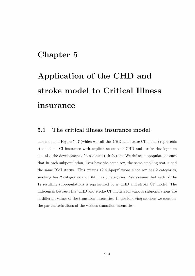
Chapter 5
Application of the CHD and
stroke model to Critical Illness
insurance
5.1 The critical illness insurance model
The model in Figure 5.47 (which we call the ‘CHD and stroke CI’ model) represents
stand alone CI insurance with explicit account of CHD and stroke development
and also the development of associated risk factors. We define subpopulations such
that in each subpopulation, lives have the same sex, the same smoking status and
the same BMI status. This creates 12 subpopulations since sex has 2 categories,
smoking has 2 categories and BMI has 3 categories. We assume that each of the
12 resulting subpopulations is represented by a ‘CHD and stroke CI’ model. The
differences between the ‘CHD and stroke CI’ models for various subpopulations are
in different values of the transition intensities. In the following sections we consider
the parameterisations of the various transition intensities.
214

chol2diab9
?λbp01
¾¾¾¾
chol2bp1
??
10
λbp12
λdiab
????
bp1, diab
chol111
?
©©©©©©©©¼
λchol12 λbp12????
bp2chol1
12
??
©©©©©©©©¼λchol12
λbp23
λdiab
????
bp2diab
13
?
©©©©©©©©¼
λchol01
λbp23
???? bp3
14
- - - -
?
©©©©©©©©¼λchol01 λdiab
bp1, diab
chol215
?λbp12
¾¾¾¾ bp2
chol2
16
?
@@
@@Rλdiab λbp23
????
bp2, diab
chol117
????
©©©©©©©©¼
HHHHHHHHjλbp23λchol12
bp3chol1
?
18
¡¡
¡¡ª
λdiabλchol12
????
bp3diab
19
- - - -
?λchol1
chol24
??
λdiab
λchol12
¾¾¾¾ diab
chol1
5
?
©©©©©©©©¼λbp01
λchol12
????
chol1bp16
??
©©©©©©©©¼ λbp12
λdiab
λchol12
????
bp1diab
7
?
©©©©©©©©¼λbp12
λchol01
???? bp2
8
- - - -
??
©©©©©©©©¼λbp23λdiabλchol01
chol11
-
-
-
-
? ?
HHHHHHHHjλchol12 λdiab λbp01
diab2
????
¡¡
¡¡ª
@@
@@Rλ
bp01λchol01
bp13
- - - -
??
©©©©©©©©¼λbp12λdiab
λchol01
bp2, diab
chol220
¾¾¾¾
HHHHHHHHjλbp23
bp3chol2
21
?λdiab
????
bp3, diab
chol122
- - - -
©©©©©©©©¼ λchol01
bp0chol00
¾
¾
¾
¾
©©©©©©©©¼ ?
HHHHHHHHjλchol01 λdiab λbp01
bp3, diab
chol223
?λMI
x+t,s,w,b=3,d=1,c=2
--
-
CHD24 λMI
x+t,s,w,b,d,cλMIx+t,s,w,b,d,c
Stroke25 λstroke
x+t,s,k,b,dλstrokex+t,s,k,b,d
Other CI26 λother
x+t,s,k,b,d,cλotherx+t,s,k,b,d,c
DeadλD
x+t,sλDx+t,s 27
Figure 5.47: A CHD and stroke model for Critical Illness Insurance.
215

5.2 Parameters for the model
5.2.1 Mortality
We assume that the mortality differs only by age and sex. The mortality is taken
as that of ELT15 adjusted for deaths due to cancer, heart attack, stroke, kidney
failure, multiple sclerosis, Alzheimer’s disease, Parkinson’s disease and benign brain
tumour. For females this means the mortality is
λDx,s=1 = (1− φf
x)λELT15Fx
where φfx is given by Equation (3.37). Similar to Equation (3.36) we define, for
males,
φmx =
θDx
θELT15Mx
where θDx and θELT15M
x are derived from O.P.C.S. (1991b), O.P.C.S. (1993b),
O.P.C.S. (1993c) and O.N.S. (1997a). The values are given in Table 5.104. The
factor φmx is smoothed, using unweighted least squares, by the function
φmx =
1.8541× 10⁻² + 6.5572× 10⁻² × x− 6.6711× 10⁻³ × x2
+2.2397× 10⁻⁴ × x3 − 2.2836× 10⁻⁶ × x4 : x ≤ 30
−2.0969 + 1.0683× 10⁻¹ × x− 1.2252× 10⁻³ × x2+
4.0118× 10⁻⁶ × x3 : x ≥ 44
with linear blending for 30 < x < 44. Figure 5.48 shows the crude and smoothed
adjustment factors. The adjusted mortality is λDx,s=0 = (1− φm
x )λELT15Mx .
5.2.2 Onset of risk factors
The transition intensities λbp01, λbp12, λbp23, λchol01, λchol12 and λdiab represent the
incidence of the risk factors hypertension, hypercholesterolaemia and diabetes. They
are given by the models described in Sections 4.6.3, 4.6.4 and 4.6.5.
216
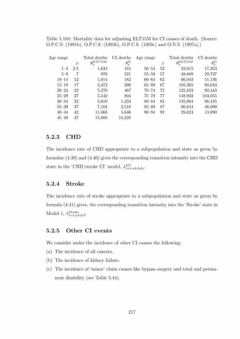
Table 5.104: Mortality data for adjusting ELT15M for CI causes of death. (Source:O.P.C.S. (1991b), O.P.C.S. (1993b), O.P.C.S. (1993c) and O.N.S. (1997a).)
Age range Total deaths CI deaths Age range Total deaths CI deathsx θELT15M
x θDx x θELT15M
x θDx
1–4 2.5 1,634 184 50–54 52 23,915 17,3535–9 7 976 221 55–59 57 38,889 29,737
10–14 12 1,014 182 60–64 62 66,043 51,13615–19 17 3,472 300 65–69 67 105,365 80,04320–24 22 5,270 467 70–74 72 125,823 92,44325–29 27 5,542 804 75–79 77 148,932 103,05530–34 32 5,610 1,233 80–84 82 135,084 86,44535–39 37 7,104 2,510 85–89 87 80,844 46,09940–44 42 11,068 5,646 90–94 92 28,624 13,89045–49 47 15,860 10,228
5.2.3 CHD
The incidence rate of CHD appropriate to a subpopulation and state as given by
formulae (4.39) and (4.40) gives the corresponding transition intensity into the CHD
state in the ‘CHD/stroke CI’ model, λMIx+t,s,k,b,d,c.
5.2.4 Stroke
The incidence rate of stroke appropriate to a subpopulation and state as given by
formula (4.41) gives, the corresponding transition intensity into the ‘Stroke’ state in
Model 1, λStrokex+t,s,k,b,d.
5.2.5 Other CI events
We consider under the incidence of other CI causes the following:
(a) The incidence of all cancers.
(b) The incidence of kidney failure.
(c) The incidence of ‘minor’ claim causes like bypass surgery and total and perma-
nent disability (see Table 3.44).
217
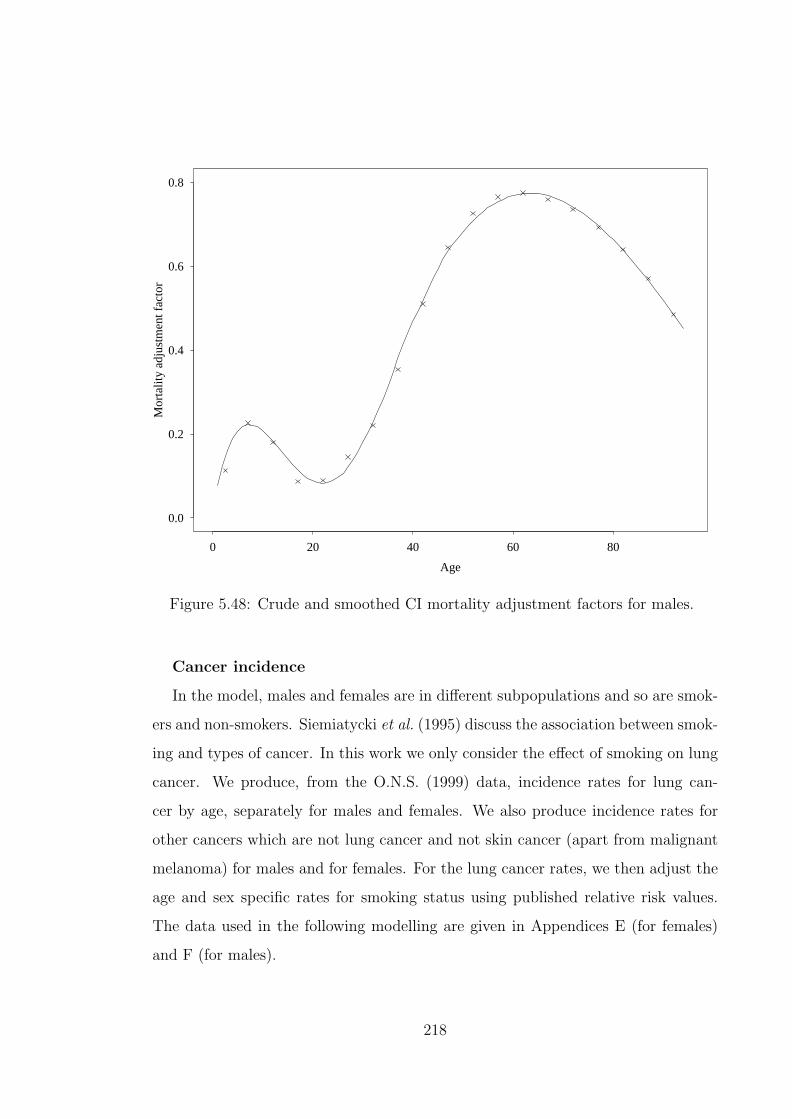
Age
Mor
talit
y ad
just
men
t fac
tor
0 20 40 60 80
0.0
0.2
0.4
0.6
0.8
Figure 5.48: Crude and smoothed CI mortality adjustment factors for males.
Cancer incidence
In the model, males and females are in different subpopulations and so are smok-
ers and non-smokers. Siemiatycki et al. (1995) discuss the association between smok-
ing and types of cancer. In this work we only consider the effect of smoking on lung
cancer. We produce, from the O.N.S. (1999) data, incidence rates for lung can-
cer by age, separately for males and females. We also produce incidence rates for
other cancers which are not lung cancer and not skin cancer (apart from malignant
melanoma) for males and for females. For the lung cancer rates, we then adjust the
age and sex specific rates for smoking status using published relative risk values.
The data used in the following modelling are given in Appendices E (for females)
and F (for males).
218

Females
For the three year investigation period 1990 to 1992, there were 35,372 cases of
lung cancer whose behaviour is given as malignant and at primary site. These apply
to ages between 30 and 88. There were 46,516,070 life-years of exposure for the
period, calculated using the census method and the population estimates for the
years 1989 to 1993 (see Section 2.5.2 for details of the calculation method). Figure
5.49 shows the crude incidence rates and the fitted function. The fitted function is
given by
f(x)lung females =
exp(α0 + α1 × x + α2 × x2) : x ≤ 60
β0 + β1 × x + β × x2 : x > 65
with linear blending between ages 60 and 65 and the coefficients are given in Table
5.105.
The two components of the function were fitted separately using weighted least
squares and in Table I.134 (Appendix I) we give the variance-covariance matrices
associated with the two sets of estimated parameters.
Table 5.105: Coefficients for fitting lung cancer incidence for females.
Coefficient Value St. Error t-valueFor x ≤ 60 :α0 −19.13 7.282× 10⁻¹ −26.27α1 2.877× 10⁻¹ 2.760× 10⁻² 10.43α2 −1.431× 10⁻³ 2.582× 10⁻⁴ −5.542
For x ≥ 65 :β0 −2.484× 10⁻² 8.708× 10⁻⁴ −28.53β1 7.101× 10⁻⁴ 2.431× 10⁻⁵ 29.22β2 −4.686× 10⁻⁶ 1.678× 10⁻⁷ −27.93
The incidence rates shown in Figure 5.49 show a decline in the incidence at the
older ages. This is mainly due to a cohort effect since the women at the older ages
are unlikely to have been affected by the large rises in smoking in the mid 1900’s).
It will be seen later that the fall in lung cancer incidence rates is less pronounced in
males. We note that this feature of falling incidence rates at the older ages is not
219

Age
Inci
denc
e ra
te
0 20 40 60 80
0.0
0.00
050.
0010
0.00
150.
0020
Figure 5.49: The incidence of lung cancer in females.
found in the incidence rates of all cancers combined. Some features of lung cancer
are that it is usually diagnosed late and is rapidly fatal.
All the other cancers considered for females had 258,756 cases and the crude rates
were smoothed using the function
f(x)other females =
exp(α0 + α1 × x + α2 × x2) : x ≤ 52
exp(β0 + β1 × x + β2 × x2) : x > 52
.
The coefficients are given in Table 5.106. The variance-covariance matrices as-
sociated with the two sets of estimated parameters are also given in Table I.134
(Appendix I).
We note that the crude rates are elevated between ages 50 and 64 due to the
effect of breast cancer screening between those ages. The effect of breast cancer
screening was discussed in Section 2.5.2. We also recall the discussion in Section
3.1.3 on the reasons for not adjusting the denominator for the prevalence of cancers
220

Table 5.106: Coefficients for fitting ‘Other cancers’ incidence for females.
Coefficient Value St. Error t-valueFor x ≤ 52 :α0 −11.78 3.513× 10⁻¹ −33.54α1 1.773× 10⁻¹ 1.679× 10⁻² 10.56α2 −1.052× 10⁻³ 1.977× 10⁻⁴ −5.322
For x > 52 :β0 −8.510 5.087× 10⁻¹ −16.73β1 7.262× 10⁻² 1.344× 10⁻² 5.402β2 −2.560× 10⁻⁴ 8.830× 10⁻⁵ −2.899
in the calculation of the incidence rates. The crude rates and the smoothed function
are shown in Figure 5.50.
Age
Inci
denc
e ra
te
0 20 40 60 80
0.0
0.00
50.
010
0.01
5
Figure 5.50: The incidence of other cancers in females.
Males
There were, for ages 30 to 88, 76,208 lung cancer cases and a corresponding
42,167,325 life-years of exposure for the period of investigation. The crude incidence
rates of lung cancer were smoothed using the function f(x) where
221

f(x)lung males =
exp(α0 + α1 × x + α2 × x2) : x ≤ 60
β0 ×{
ββ21
Γ(β2)e−β1xxβ2−1
}: x > 70
with linear blending between ages 60 and 70. The coefficients are given in Table
5.107. The two components of the function are fitted separately using weighted least
squares and the variance-covariance matrices are given in Table I.134 (Appendix I).
Table 5.107: Coefficients for fitting lung cancer incidence for males.
Coefficient Value St. Error t-valueFor x ≤ 60 :α0 −21.56 3.598× 10⁻¹ −59.92α1 3.945× 10⁻¹ 1.249× 10⁻² 31.58α2 −2.299× 10⁻³ 1.073× 10⁻⁴ −21.42
For x > 70 :β0 3.017× 10⁻¹ 1.050× 10⁻² 28.73β1 3.339× 10⁻¹ 1.604× 10⁻² 20.82β2 28.65 1.161 24.69
The crude rates and the fitted function are shown in Figure 5.51.
We then considered all other cancers in males and there were 216,590 cases for
the period for ages 30 to 88. The crude rates were smoothed using the function
f(x)other males =
exp(α0 + α1 × x) : x ≤ 55
exp(β0 + β1 × x + β2 × x2) : x > 60
with linear blending between ages 55 and 60. The coefficients are given in Table
5.108. The two components of the function are fitted separately using weighted least
squares and the variance-covariance matrices are also given in Table I.134 (Appendix
I).
The crude rates and smooth function are shown in Figure 5.52
Adjustment for smoking in lung cancer incidence
Based on a study of 857 cases and 2,238 controls in Canada, Siemiatycki et al.
(1995) estimate that the relative risk of lung cancer in people who have ever smoked
222
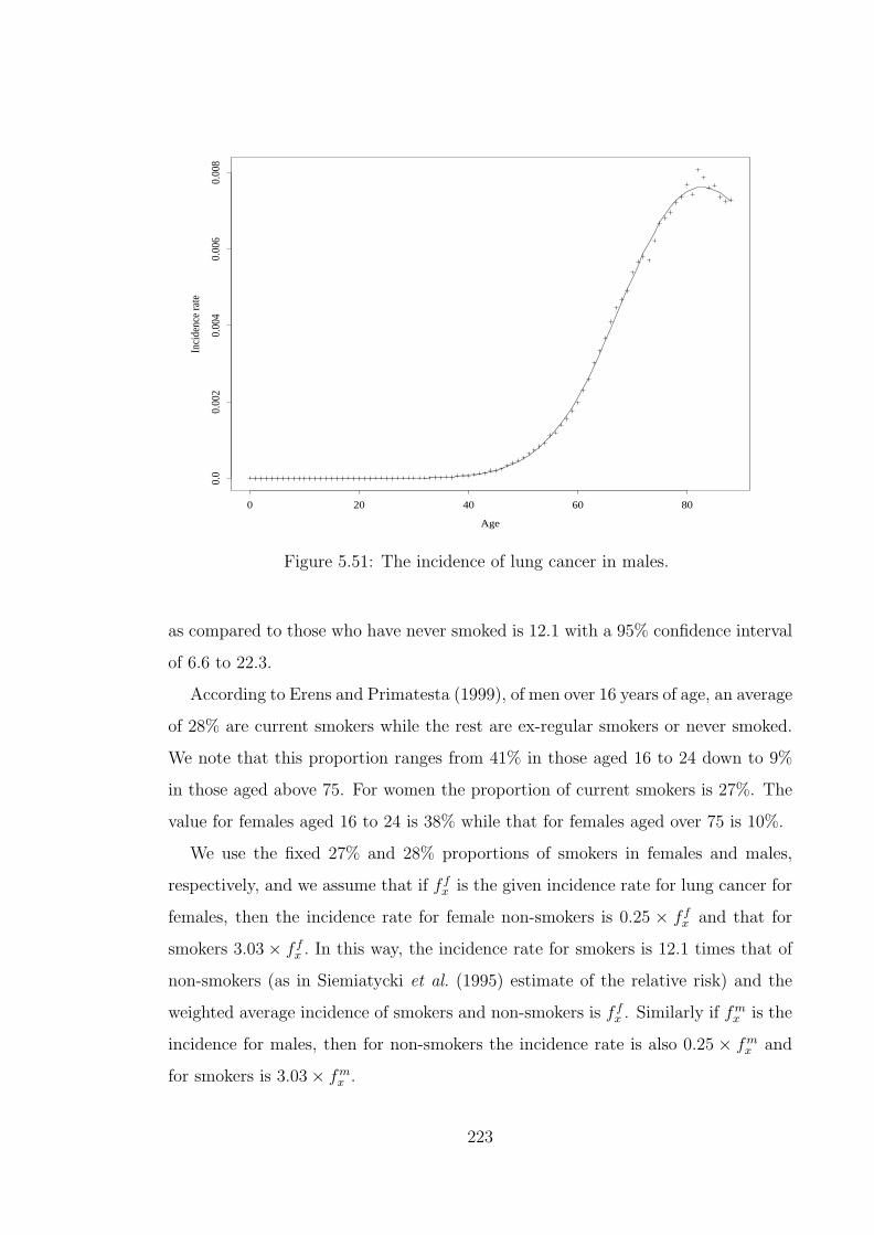
Age
Inci
denc
e ra
te
0 20 40 60 80
0.0
0.00
20.
004
0.00
60.
008
Figure 5.51: The incidence of lung cancer in males.
as compared to those who have never smoked is 12.1 with a 95% confidence interval
of 6.6 to 22.3.
According to Erens and Primatesta (1999), of men over 16 years of age, an average
of 28% are current smokers while the rest are ex-regular smokers or never smoked.
We note that this proportion ranges from 41% in those aged 16 to 24 down to 9%
in those aged above 75. For women the proportion of current smokers is 27%. The
value for females aged 16 to 24 is 38% while that for females aged over 75 is 10%.
We use the fixed 27% and 28% proportions of smokers in females and males,
respectively, and we assume that if f fx is the given incidence rate for lung cancer for
females, then the incidence rate for female non-smokers is 0.25 × f fx and that for
smokers 3.03× f fx . In this way, the incidence rate for smokers is 12.1 times that of
non-smokers (as in Siemiatycki et al. (1995) estimate of the relative risk) and the
weighted average incidence of smokers and non-smokers is f fx . Similarly if fm
x is the
incidence for males, then for non-smokers the incidence rate is also 0.25 × fmx and
for smokers is 3.03× fmx .
223

Table 5.108: Coefficients for fitting ‘Other cancers’ incidence for males.
Coefficient Value St. Error t-valueFor x ≤ 55 :α0 −11.02 7.736× 10⁻² −142.5α1 9.621× 10⁻² 1.506× 10⁻³ 63.87
For x > 60 :β0 −16.37 1.795× 10⁻¹ −91.16β1 2.725× 10⁻¹ 5.058× 10⁻³ 53.88β2 −1.443× 10⁻³ 3.529× 10⁻⁵ −40.89
Kidney failure
Kidney failure is one of the end-points covered under critical illness policies. The
U.K. insurance industry’s definition of kidney failure is
“End-stage renal failure (ESRD) presenting as chronic irreversible failure of both
kidneys to function, as a result of which either regular renal dialysis or renal transplant
is required.”
These two forms of treatment for ESRD mentioned in the definition are referred to
as renal replacement therapy (RRT).
American Diabetes Association: Clinical Practice Recommendations 2000 (2000)
state that nephropathy leading to kidney failure is one of the long-term complica-
tions of diabetes mellitus. Our model for CHD stroke and CI explicitly models the
influence of diabetes on insurance costs and therefore we should consider the differ-
ence between incidence rates of kidney failure between diabetics and non-diabetics.
This is in contrast to the approach for the CI model applied to BCOC in which we
considered renal failure as part of ‘other CI’ claim causes.
To parameterize the incidence rates of kidney failure we use data mainly from
the U.S. Renal Data System (USRDS) 1999 Annual Data Report (U.S. Renal Data
System (1999)). For the years 1994 to 1997 combined, the data includes the number
of new cases of patients requiring RRT subdivided by the primary disease causing
the ESRD. These primary causes include diabetes, hypertension, glomerulonephritis,
cystic kidney disease and other urologic diseases. Diabetes is the largest single cause
of ESRD. They also give the corresponding population figures for the U.S.A. states
224
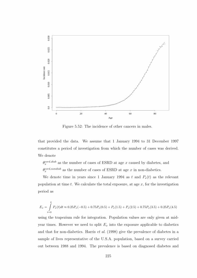
Age
Inci
denc
e ra
te
0 20 40 60 80
0.0
0.00
50.
010
0.01
50.
020
0.02
50.
030
Figure 5.52: The incidence of other cancers in males.
that provided the data. We assume that 1 January 1994 to 31 December 1997
constitutes a period of investigation from which the number of cases was derived.
We denote
θesrd diabx as the number of cases of ESRD at age x caused by diabetes, and
θesrd nondiabx as the number of cases of ESRD at age x in non-diabetics.
We denote time in years since 1 January 1994 as t and Px(t) as the relevant
population at time t. We calculate the total exposure, at age x, for the investigation
period as
Ex =
4∫t=0
Px(t)dt ≈ 0.25Px(−0.5) + 0.75Px(0.5) + Px(1.5) + Px(2.5) + 0.75Px(3.5) + 0.25Px(4.5)
using the trapezium rule for integration. Population values are only given at mid-
year times. However we need to split Ex into the exposure applicable to diabetics
and that for non-diabetics. Harris et al. (1998) give the prevalence of diabetes in a
sample of lives representative of the U.S.A. population, based on a survey carried
out between 1988 and 1994. The prevalence is based on diagnosed diabetes and
225

undiagnosed diabetes. Undiagonised diabetes is defined as blood sugar level ex-
ceeding 126mg/dL in lives without a previous diagnosis of diabetes. The definition,
combining diagnosed and undiagnosed diabetes, is comparable with the definition
of diabetes that we use in our modelling. The prevalence rate estimates given by
Harris et al. (1998) are shown in Table 5.109
Table 5.109: Prevalence of diabetes (as % of population) in men and women in theU.S.A. population. Source ( Harris et al. (1998).)
Age group20-39 40-49 50-59 60-74 75+
Males 1.6 6.8 12.9 20.2 21.1Females 1.7 6.1 12.4 17.8 17.5
We represent the prevalence of diabetes by
exp(−8.887 + 0.1967x− 0.001313x2
)for males and
exp(−9.0211 + 0.2019x− 0.001387x2
)for females, where x represents age at the last birthday. These functions are derived
by unweighted least squares fitting of the data in Table 5.109 using the mid-point
ages of the age groups. The estimated prevalence rates together with the fitted
functions are shown in Figure 5.53
We can then split Ex into the exposure for diabetics Ediabx and that for non-
diabetics Enondiabx in proportions given by the prevalence functions.
For lives with diabetes we note that the incidence of kidney failure depends on
whether the life has Type 1 or Type 2 diabetes (Stephens et al. (1990)). Therefore
we need to split our exposure Ediabx into the exposures E1
x and E2x for Type 1 and
Type 2 diabetics respectively.
We need to know, for the ages of interest, the proportion of diabetics who are
Type 1. There is little published about the age and sex specific proportions of
Type 1 diabetics among all diabetics. Table 5.110 shows the prevalence of Insulin
Dependent Diabetes Mellitus (IDDM) diagnosed at ages above 30 as a proportion
226

Males
Age
Dia
bete
s pr
eval
ence
20 30 40 50 60 70 80
0.0
0.05
0.10
0.15
0.20
0.25
Females
Age
Dia
bete
s pr
eval
ence
20 30 40 50 60 70 800.
00.
050.
100.
150.
200.
25
Figure 5.53: The crude and fitted prevalence rates for diabetes.
of all diabetes diagnoses at ages above 30. Type 1 diabetes is the new term for
IDDM. The values in Table 5.110 would understate the actual prevalence since they
do not consider diagnosed at ages below 30. We assume that the prevalence values
are equally applicable to both males and females.
Table 5.110: The prevalence of IDDM as a proportion of people with diabetes diag-nosed at ages 30–74 of age. Source ( Harris and Robbins (1994).)
Age group 30–49 50–64 65–74Prevalence 0.085 0.074 0.068
In order to evaluate the incidence of ESRD in diabetics we also need to split the
number of cases θesrd diabx into θesrd 1
x and θesrd 2x . There is also very little published
data to use for this subdivision. The data in Table 5.111 shows the number of ESRD
cases due to diabetes and how they are distributed by type of diabetes over some
broad age groups.
227

Table 5.111: Characteristics of ESRD due to diabetes. (Source: USRDS AnnualReports 1997–2001.)
Period Number of cases due to % of cases due % due to Type 1 at agesType 1 Type 2 to Type 1 < 20 20–64 > 64
1991–1995 47,839 68,099 41% 56% 48% 32%1992–1996 46,100 84,373 35% 50% 42% 26%1993–1997 41,521 102,333 29% 50% 36% 20%1994–1998 33,818 118,626 22% 42% 30% 13%1995–1999 23,390 144,601 16%
The values in Table 5.111 show a marked decline in the proportion of cases due to
Type 1 diabetes in the total number of cases due to diabetes. The USRDS reports
that since 1992 the number of cases of ESRD due to diabetes has been increasing
at a rate of 9% per annum (U.S. Renal Data System (1999)). We suspect that
this increase in ESRD cases due to diabetes is largely due to an increase in Type
2 diabetes cases (the underlying disease or its diagnosis). This would be consistent
with the pattern seen in Table 5.111 in which the proportional contribution of Type
1 diabetes falls.
Given that our period of investigation is 1994 to 1997, we assume that the dis-
tribution of ESRD cases due to each type of diabetes is given by that of 1994 to
1998 in Table 5.111. To avoid any possible distortions due to the wide age groups
used in Table 5.111 we assume that the proportion of cases due to Type 1 changes
linearly with age with 30% being applicable at exact age 42 and 13% at exact age
75. Therefore the proportion is represented by 0.5163−0.00515x where x is the age.
We then split θesrd diabx into ESRDθesrd 1
x and θesrd 2x using these proportions as well
as assuming that Type 1 and Type 2 diabetes are the only types of diabetes. The
data we obtain for non-diabetics, Type 1 diabetics and Type 2 diabetics are shown
in Appendix J.
The crude incidence rates of ESRD for non-diabetics, Type 1 diabetics and Type
2 diabetics are calculated as
λesrd nondiabx =
θesrd nondiabx
Enondiabx
, λesrd 1x =
θesrd 1x
E1x
and λesrd 2x =
θesrd 2x
E2x
228
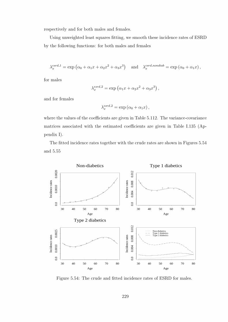
respectively and for both males and females.
Using unweighted least squares fitting, we smooth these incidence rates of ESRD
by the following functions: for both males and females
λesrd 1x = exp
(α0 + α1x + α2x
2 + α3x3)
and λesrd nondiabx = exp (α0 + α1x) ,
for males
λesrd 2x = exp
(α1x + α2x
2 + α3x3),
and for females
λesrd 2x = exp (α0 + α1x) ,
where the values of the coefficients are given in Table 5.112. The variance-covariance
matrices associated with the estimated coefficients are given in Table I.135 (Ap-
pendix I).
The fitted incidence rates together with the crude rates are shown in Figures 5.54
and 5.55
Non-diabetics
Age
Inci
denc
e ra
tes
30 40 50 60 70 80
0.0
0.00
100.
0020
Type 1 diabetics
Age
Inci
denc
e ra
tes
30 40 50 60 70 80
0.0
0.00
40.
008
0.01
2
Type 2 diabetics
Age
Inci
denc
e ra
tes
30 40 50 60 70 80
0.0
0.00
100.
0025
Age
Inci
denc
e ra
tes
30 40 50 60 70 80
0.0
0.00
40.
008
0.01
2
Non-diabeticsType 1 diabeticsType 2 diabetics
Figure 5.54: The crude and fitted incidence rates of ESRD for males.
229

Table 5.112: Coefficients for fitting kidney failure incidence.
Coefficient Value St. Error t-valueMales:
Non-diabeticα0 −11.5513 1.572× 10⁻¹ −73.48α1 6.509× 10⁻² 2.184× 10⁻³ 29.81
Type 1 diabeticsα0 4.3868 1.120 3.916α1 −5.689× 10⁻¹ 6.860× 10⁻² −8.292α2 1.103× 10⁻² 1.341× 10⁻³ 8.226α3 −6.952× 10⁻⁵ 8.433× 10⁻⁶ −8.244
Type 2 diabeticsα1 −4.194× 10⁻¹ 3.452× 10⁻³ −121.48α2 8.330× 10⁻³ 1.189× 10⁻⁴ 70.04α3 −5.136× 10⁻⁵ 1.002× 10⁻⁶ −51.25
Females:Non-diabetic
α0 −12.1810 1.487× 10⁻¹ −81.94α1 6.489× 10⁻² 2.065× 10⁻³ 31.42
Type 1 diabeticsα0 3.6856 1.763 2.090α1 −5.675× 10⁻¹ 1.033× 10⁻¹ −5.495α2 1.087× 10⁻² 1.925× 10⁻³ 5.649α3 −6.491× 10⁻⁵ 1.153× 10⁻⁵ −5.632
Type 2 diabeticsα0 −8.9406 1.934× 10⁻¹ −46.23α1 4.141× 10⁻² 2.811× 10⁻³ 14.73
In Table 5.113 we show the crude incidence rates of ESRD for the ages below
64 from our data and compare them to those given by Stephens et al. (1990). The
values show very good agreement between the incidence rates for ESRD due to
Type 1 diabetes. Our data have much higher incidence rates for ESRD due to
Type 2 diabetes than Stephens et al. (1990). Given that the results from Stephens
et al. (1990) relate to the years 1983 to 1984, we feel the comparison is consistent
with stable rates of ESRD due to Type 1 diabetes and with rates of ESRD due to
Type 2 diabetes sharply rising over the years. We feel that having results which
are consistent with Stephens et al. (1990) indicates that our overall split of the
exposure and the number of cases into those applicable to Type 1 and Type 2
diabetes is reasonable. However there is still uncertainty as to the reasonableness
of the distribution of the cases by age. Age specific numbers of ESRD cases due to
Type 1 would enable us to be more confident about the relationship of the incidence
230
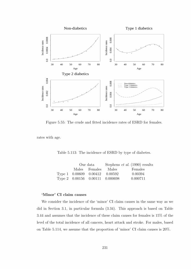
Non-diabetics
Age
Inci
denc
e ra
tes
30 40 50 60 70 80
0.0
0.00
040.
0008
Type 1 diabetics
Age
Inci
denc
e ra
tes
30 40 50 60 70 80
0.0
0.00
40.
008
Type 2 diabetics
Age
Inci
denc
e ra
tes
30 40 50 60 70 80
0.0
0.00
20.
004
Age
Inci
denc
e ra
tes
30 40 50 60 70 800.
00.
004
0.00
8
Non-diabeticsType 1 diabeticsType 2 diabetics
Figure 5.55: The crude and fitted incidence rates of ESRD for females.
rates with age.
Table 5.113: The incidence of ESRD by type of diabetes.
Our data Stephens et al. (1990) resultsMales Females Males Females
Type 1 0.00609 0.00412 0.00592 0.00394Type 2 0.00156 0.00111 0.000698 0.000711
‘Minor’ CI claim causes
We consider the incidence of the ‘minor’ CI claim causes in the same way as we
did in Section 3.1, in particular formula (3.34). This approach is based on Table
3.44 and assumes that the incidence of these claim causes for females is 15% of the
level of the total incidence of all cancers, heart attack and stroke. For males, based
on Table 5.114, we assume that the proportion of ‘minor’ CI claim causes is 20%.
231

Table 5.114: Incidence rates (per 1,000) of CI claims by cause, for males in the U.K.in 1991–97. (Source: Dinani et al. (2000).)
Incidence Rate per 1,000 at AgeCause ≤ 30 31–40 41–50 51–60 ≥ 61Cancer 0.371 0.608 1.196 3.062 10.816Heart Attack 0.015 0.172 1.088 2.932 5.408Stroke 0.049 0.104 0.208 0.812 2.028Bypass Surgery 0.005 0.019 0.203 0.830 1.859Multiple Sclerosis 0.034 0.083 0.095 0.037 0.000Total Permanent Disability 0.039 0.057 0.153 0.664 0.338Other 0.034 0.072 0.077 0.129 1.859Total 0.547 1.117 3.020 8.465 22.309
Therefore for the ‘CHD and stroke CI’ model, the transition intensity for ‘Other
CI’ is given as:
λOtherx+t,s=0,k=0,b,d,c = 1.20
{0.25× f(x + t)lung males + f(x + t)other males
}+0.20{λCHD
x+t,s=0,k=0,b,d,c + λstrokex+t,s=0,k=0,b,d}+ λesrd
x+t ,
for males, non-smokers,
λOtherx+t,s=0,k=1,b,d,c = 1.20
{3.03× f(x + t)lung males + f(x + t)other males
}+0.20{λCHD
x+t,s=0,k=1,b,d,c + λstrokex+t,s=0,k=1,b,d}+ λesrd
x+t ,
for males, smokers,
λOtherx+t,s=1,k=0,b,d,c = 1.15
{0.25× f(x + t)lung females + f(x + t)other females
}+0.15{λCHD
x+t,s=1,k=0,b,d,c + λstrokex+t,s=1,k=0,b,d}+ λesrd
x+t ,
for females, non-smokers, and
λOtherx+t,s=1,k=1,b,d,c = 1.15
{3.03× f(x + t)lung females + f(x + t)other females
}+0.15{λCHD
x+t,s=1,k=1,b,d,c + λstrokex+t,s=1,k=1,b,d}+ λesrd
x+t ,
for females, smokers.
232

5.3 Costs of critical illness insurance
We consider the ‘CHD and stroke CI’ model in Figure 5.47. For an individual life
the states labelled ‘Diabetes’ represent one of Type 1 diabetes and Type 2 diabetes
since a life can, normally, be affected by only one of them. We consider the incidence
of diabetes, λdiab, as representing the sum of the incidence of Type 1 diabetes and
of Type 2 diabetes. Based on the prevalence of Type 1 diabetes diagnosed after
the age of 30 years (given in Table 5.110 ) we assume that the incidence of Type 1
diabetes is 0.085× λdiab and the incidence of Type 2 diabetes is 0.915× λdiab at all
ages.
In this model we assume that the incidence of cardiovascular disorders is not
dependent on the type of diabetes. We have not seen literature that indicates that
the incidence of CHD or stroke in Type 1 diabetics is significantly different from
that in Type 2 diabetics and give age specific differentials in the incidence rates.
Figure 5.47 is a Markov model and, using the results of Norberg (1995) sum-
marised in Section 1.3, we can calculate any moments of the present value of
(a) a benefit payable on transition into any of the states numbered 24 to 26, and
(b) a premium payable continuously while in any of the transient states numbered
0 to 23 in Figure 5.47.
Similar to the assumptions used in Section 3.2, we use a value of δ = 0.05 in
solving Thiele’s differential equation. In these calculations the transition intensities
into the CHD and stroke states are adjusted for the 28-day survival requirement for
CI claims to be valid. Therefore the transition intensity into the CHD state is given
by pheartx × λMI
x+t,s,k,b,d,c where pheartx is given by Equation (3.29). The corresponding
transition intensity for stroke is pstrokex ×λstroke
x+t,s,k,b,d where pstrokex is given by Equation
(3.32). Consequently, the force of mortality is adjusted so that it is
λDx+t,s + (1− pheart
x )× λMIx+t,s,k,b,d,c + (1− pstroke
x )× λstrokex+t,s,k,b,d.
233

5.3.1 Premium rating by subpopulation and risk factor sta-
tus
We consider the lives in the ‘Males, non-smoker, normal BMI’ subpopulation, and
in state 0 of the corresponding ‘CHD and stroke CI’ model (Figure 5.47) as our
baseline population. Firstly we discuss the level of the risk associated with the
baseline population and then we look at the risk differentials of other subpopulations
and states with reference to this chosen baseline.
Premium levels
For various ages at entry and terms of CI policies we can calculate the expected
present value (EPV) of an annuity payable continuously until the end of the term
or earlier claim event or death. We can also calculate the EPV of a benefit of £1
payable on transition to the CI claim states. We define the level net premium as
the level of the annuity payment that makes the EPV of the loss ( EPV of benefit –
EPV of annuity) equal to zero. The premiums for the baseline group are shown in
Table 5.115. As we would expect, for a fixed term the premiums increase with the
age at entry and for a fixed age at entry, the premiums increase with the term of
the policy.
We also show in Table 5.115 the standard deviation of the present value (PV) of
the loss associated with the premium and the corresponding skewness. The skewness
values are all negative which suggests that the PV’s of the loss are largely positive
with a small probability of very large negative PV’s.
The level net premiums shown in Table 5.115 are based on the estimates of pa-
rameter values for the incidence rate models that are described in Chapter 4 and
the earlier sections of this chapter. In all, apart from the adjustments for mortality,
we use 48 least squares estimates in the calculation of incidence rates of cancers,
CHD, stroke, blood pressure, hypercholesterolaemia, diabetes and kidney failure for
males. There are 49 estimates used for females, 19 of which are common to both
sexes. These parameter values represent the estimated means of the corresponding
estimators, given the data. The variation and correlation associated with the estima-
tors are contained in the estimate of the variance-covariance matrix. The variance
234

Table 5.115: Premium details for CI cover of £1 for non-smoking males with ‘normal’BMI.
Age 35 at Entry Age 45 at Entry Age 55 at EntryTerm Term Term Term Term Term10 Yrs 20 Yrs 30 Yrs 10 Yrs 20 Yrs 10 Yrs
Level netpremium 0.00250 0.00362 0.00521 0.00514 0.00764 0.01139
Standard deviation ofpresent value of loss 0.1229 0.1622 0.1833 0.1744 0.2285 0.2540Skewness ofpresent value of loss −6.26 −3.69 −2.57 −4.23 −2.33 −2.63
Mean of simulatedpremiums 0.00253 0.00366 0.00525 0.00518 0.00769 0.01144Standard deviation ofsimulated premiums 0.00025 0.00028 0.00030 0.00033 0.00037 0.00047
will reflect the uncertainty of the mean parameter estimates and is dependent on
the amount of data used to calculate the estimates. We need to assess how any
such uncertainty in the data used to parameterise our model may affect the level
net premiums.
We assume that our estimators are normally (or multivariate normally) dis-
tributed, their mean is given by the estimated mean (vector of means) and the
variance is given by the estimated variance (variance-covariance matrix). This en-
ables us to draw samples of parameter values from these distributions such that the
sampled values will have the same mean, variance and correlations as our estimators.
We let A represent the vector of estimated means of the estimators, and V
the estimated variance-covariance matrix. From V we can derive a ‘square root’
decomposition L such that LLT = V. LT is an upper triangular matrix called the
Cholesky decomposition of V (see Conte and de Boor (1980)). For a vector R of
deviates from a normal distribution with mean 0 and variance 1, RLT + A produces
a vector of values from a distribution with mean A and variance and correlations
given by V. We applied this method, using the variance-covariance matrices given
in Appendix I to derive 9, 999 sets of parameter values. These sets were used to
calculate 9, 999 premium values for the 5 policy scenarios we are considering. The
mean values of these premiums and the standard deviations are also shown in Table
235

5.115. It shows that the means of the premiums are very close to the premiums
based on the estimated means of the parameter estimators. It can be seen from
Figure 5.56 that the distributions of the premiums are approximately symmetric
around the means of the premiums.
Age 35 years, term 10 years
Level net premium0.0020 0.0025 0.0030 0.0035
0.0
0.05
0.10
0.15
0.20
Age 35 years, term 20 years
Level net premium0.0030 0.0035 0.0040 0.0045 0.0050
0.0
0.05
0.10
0.15
Age 35 years, term 30 years
Level net premium0.0045 0.0050 0.0055 0.0060 0.0065
0.0
0.05
0.10
0.15
Age 45 years, term 10 years
Level net premium0.0040 0.0045 0.0050 0.0055 0.0060 0.0065
0.0
0.05
0.10
0.15
Age 45 years, term 20 years
Level net premium0.0065 0.0070 0.0075 0.0080 0.0085 0.0090
0.0
0.04
0.08
0.12
Age 55 years, term 10 years
Level net premium0.0100 0.0105 0.0110 0.0115 0.0120 0.0125
0.0
0.04
0.08
0.12
Figure 5.56: Probability distribution of simulated level net premium values of CIpolicies of £1 cover for non-smoking males with ‘normal’ BMI. The dashed verticallines represent the level net premium calculated using the means of the parameterestimates and the solid vertical lines represent the means of the simulated level netpremiums.
Premium differentials
Within the subpopulation of non-smoking males with ‘normal’ BMI, we need to
assess how the risk (as measured by the rating) changes for different risk profiles
at policy inception, i.e. for different starting states in Figure 5.47. In Table 5.116
we show the ratings relative to the baseline level net premiums previously given in
Table 5.115.
236

Table 5.116: Premium ratings for CI cover of £1 for non-smoking males with ‘normal’BMI.
Age at Entry35 35 35 45 45 55
Risk factors Term (in Years) 10 20 30 10 20 10% % % % % %
‘Moderate’ chol +4 +5 +5 +3 +4 +2Type 1 diab +247 +168 +117 +118 +82 +61Type 2 diab +60 +44 +33 +36 +27 +22‘High normal’ b.p. +6 +10 +11 +6 +8 +5‘High’ chol +33 +27 +21 +24 +19 +16‘Moderate’ chol and Type 1 diab +251 +174 +123 +122 +86 +63‘Moderate’ chol and Type 2 diab +65 +51 +39 +39 +31 +24‘Moderate’ chol and ‘High normal’ b.p. +11 +16 +17 +9 +13 +7‘High normal’ b.p. and Type 1 diab +255 +181 +130 +126 +92 +67‘High normal’ b.p. and Type 2 diab +68 +57 +46 +43 +37 +29‘Hypertension Stage I’ +43 +40 +34 +33 +30 +24‘High’ chol and Type 1 diab +290 +203 +143 +150 +106 +82‘High’ chol and Type 2 diab +103 +79 +60 +67 +51 +44‘High’ chol and ‘High normal’ b.p. +44 +43 +37 +34 +32 +24‘High normal’ b.p., ‘Moderate’ chol, Type 1 diab +260 +189 +137 +130 +98 +69‘High normal’ b.p., ‘Moderate’ chol, Type 2 diab +74 +65 +54 +48 +43 +31‘Hypertension Stage I’ and ‘Moderate’ chol +49 +49 +43 +38 +37 +27‘Hypertension Stage I’ and Type 1 diab +303 +220 +160 +161 +120 +92‘Hypertension Stage I’ and Type 2 diab +116 +96 +77 +79 +65 +53‘Hypertension Stage II-III’ +97 +82 +65 +79 +64 +62‘High’ chol, ‘High normal’ b.p., Type 1 diab +304 +222 +162 +162 +121 +91‘High’ chol, ‘High normal’ b.p., Type 2 diab +117 +99 +79 +79 +67 +53‘High’ chol and ‘Hypertension Stage I’ +103 +90 +72 +77 +65 +54‘Hypertension Stage I’, ‘Moderate’ chol and Type 1 diab +311 +231 +170 +168 +128 +96‘Hypertension Stage I’, ‘Moderate’ chol and Type 2 diab +124 +108 +87 +85 +73 +57‘Hypertension Stage II-III’ and ‘Moderate’ chol +106 +94 +76 +86 +72 +65‘Hypertension Stage II-III’ and Type 1 diab +376 +276 +201 +224 +166 +144‘Hypertension Stage II-III’ and Type 2 diab +189 +153 +118 +142 +111 +105‘Hypertension Stage I’, and ‘High’ chol and Type 1 diab +381 +283 +207 +219 +164 +130‘Hypertension Stage I’, and ‘High’ chol and Type 2 diab +195 +160 +124 +136 +109 +92‘Hypertension Stage II-III’ and ‘High’ chol +183 +149 +115 +142 +111 +103‘Hypertension Stage II-III’, ‘Moderate’ chol, Type 1 diab +388 +291 +213 +233 +176 +149‘Hypertension Stage II-III’, ‘Moderate’ chol, Type 2 diab +201 +168 +131 +151 +121 +110‘Hypertension Stage II-III’, ‘High’ chol and Type 1 diab +489 +362 +263 +305 +224 +198‘Hypertension Stage II-III’, ‘High’ chol and Type 2 diab +302 +239 +180 +223 +170 +159
chol = cholesterol, b.p.= blood pressure, diab = diabetes
237

We note the following about the ratings in Table 5.116:
(a) For the younger ages, the single risk factor with the highest rating is Type 1
diabetes, while for the older ages the highest rating is associated with blood
pressure (Hypertension Stage II-III).
(b) There is a significant difference in risk for lives with different risk profiles. The
highest risk is always associated with lives who have ‘High cholesterol’, ‘Hyper-
tension stage II-III’ and Type 1 diabetes. The ranking of the risk for any other
combination of risk factors depends on the age at entry and the term of the
policy. The differences are mainly due to the increase, with age, in the signifi-
cance of blood pressure values on the risk and a decrease in the significance of
diabetes.
(c) For the same term, the impact of the risk factors on the ratings decreases as the
age increases. This reflects that CHD and stroke incidence increase with age
independent of the risk factors. This is in line with current underwriting practice
which considers the age of the applicant. For the blood pressure and cholesterol
risk factors, underwriting practice tends to consider narrow age ranges while
for diabetes the age distinction is generally whether the applicant is below or
above age 40. In the ratings for blood pressure and for cholesterol, older ages
have lower ratings than younger lives, for the same risk factor levels. This is
also reflected in current underwriting practice.
(d) The significance, in terms of risk, of particular factors depends on which other
factors are present. As an example, for a 10-year policy for a life aged 35, the
ratings associated with ‘High cholesterol’, ‘Hypertension stage II-III’ and Type
1 diabetes separately add up to +377 but the rating for the presence of all three
is +489. This synergy is reflected in the current underwriting practice (Pokorski
(1999) and Swiss-Re ratings).
(e) The ratings are consistent in that having an additional risk factor leads to a
higher rating.
(f) The ratings are partly consistent with current underwriting practice concern-
ing lives with Type 1 diabetes. As we mentioned before, current underwriting
238

would recommend declinature for any applicant aged under 40 who has dia-
betes. According to Table 5.116, for policies of term 10 years, these lives attract
ratings of at least +247 which is above the insurable limit. For policies of longer
terms, Type 1 diabetics under 40 years of age may be insurable depending on
which other risk factors are present. This dependence of the ratings for Type 1
diabetics on the term of the policy is largely not allowed for in current under-
writing. In the case of lives with Type 1 or Type 2 diabetes for which current
underwriting may recommend insurance rather than declinature, the policies
are supposed to be of short term, with the policy not covering ages beyond 55
years. However in Table 5.116, for policies issued to lives age 35, we find that
the ratings for diabetics decrease as the term increases.
We note that the higher costs of insurance for lives with Type 1 diabetes are
due to the high incidence of kidney failure in these lives.
(g) There is disagreement between the ratings from our model and current under-
writing practice for lives with Type 2 diabetes. Underwriting practice recom-
mends declinature in all cases of Type 2 diabetes below age 40 but our ratings
show that such lives, in certain cases, are insurable.
(h) Current underwriting uses narrower categories for blood pressure and blood
cholesterol levels, than those used in our model. This makes the comparison of
the ratings in Table 5.116 and underwriting practice ratings rather difficult. In
Table 5.117, for lives aged 35 at entry and policies of term 10 years, we show
some of the ratings from Table 5.116 and the range of possible ratings according
to current underwriting practice. We have not shown some states which include
Type 1 diabetes as declinature is recommended both by our model and by cur-
rent underwriting practice. There is some broad agreement between our model
ratings and the range of ratings currently recommended by underwriters for the
risk factors moderate cholesterol, ‘High Normal’ blood pressure, ‘Hypertension
Stage I’ and ‘Hypertension Stage II-III’ but the disparity in ratings associated
with Type 2 diabetes and ‘High’ cholesterol is also marked.
The differentials in premiums considered so far are for lives in the same sub-
population but with different risk factors. We now consider the ratings associated
239
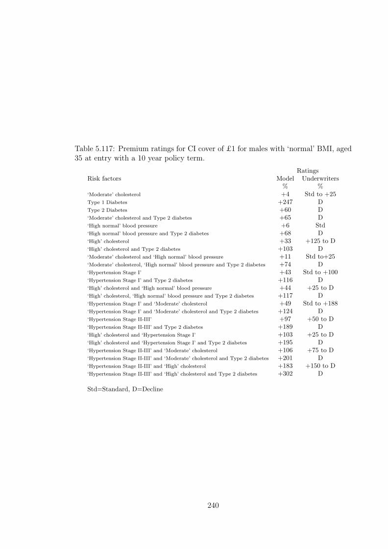
Table 5.117: Premium ratings for CI cover of £1 for males with ‘normal’ BMI, aged35 at entry with a 10 year policy term.
RatingsRisk factors Model Underwriters
% %‘Moderate’ cholesterol +4 Std to +25Type 1 Diabetes +247 DType 2 Diabetes +60 D‘Moderate’ cholesterol and Type 2 diabetes +65 D‘High normal’ blood pressure +6 Std‘High normal’ blood pressure and Type 2 diabetes +68 D‘High’ cholesterol +33 +125 to D‘High’ cholesterol and Type 2 diabetes +103 D‘Moderate’ cholesterol and ‘High normal’ blood pressure +11 Std to+25‘Moderate’ cholesterol, ‘High normal’ blood pressure and Type 2 diabetes +74 D‘Hypertension Stage I’ +43 Std to +100‘Hypertension Stage I’ and Type 2 diabetes +116 D‘High’ cholesterol and ‘High normal’ blood pressure +44 +25 to D‘High’ cholesterol, ‘High normal’ blood pressure and Type 2 diabetes +117 D‘Hypertension Stage I’ and ‘Moderate’ cholesterol +49 Std to +188‘Hypertension Stage I’ and ‘Moderate’ cholesterol and Type 2 diabetes +124 D‘Hypertension Stage II-III’ +97 +50 to D‘Hypertension Stage II-III’ and Type 2 diabetes +189 D‘High’ cholesterol and ‘Hypertension Stage I’ +103 +25 to D‘High’ cholesterol and ‘Hypertension Stage I’ and Type 2 diabetes +195 D‘Hypertension Stage II-III’ and ‘Moderate’ cholesterol +106 +75 to D‘Hypertension Stage II-III’ and ‘Moderate’ cholesterol and Type 2 diabetes +201 D‘Hypertension Stage II-III’ and ‘High’ cholesterol +183 +150 to D‘Hypertension Stage II-III’ and ‘High’ cholesterol and Type 2 diabetes +302 D
Std=Standard, D=Decline
240

with different subpopulations. These ratings are shown in Tables 5.118 and 5.119,
expressed in relation to the level net premiums given in Table 5.115. In Table 5.118
we give the ratings for lives with ‘No risk factors’ (that is in State 0 of the ‘CHD and
stroke CI’ model) but in different sex, smoking and BMI specific subpopulations.
The ratings in Table 5.119 relate to ‘Males, smokers, normal BMI’ subpopulation
considering different risk factors. We note some points from these tables.
(a) The ratings for males are different from those for females. However, these ratings
are not as high as the ratings for the very high risk states shown in Table 5.116.
(b) The ratings for smokers are different from those for non-smokers. The ratings are
also generally much lower than those for combinations of diabetes, hypertension
and hypercholesterolaemia.
One of the main differences between the ratings for smokers in Table 5.119
compared to those for non-smokers in Table 5.116 is that for states without
diabetes the ratings for smokers do not fall much as either age or term increases.
Indeed for the states with fewer risk factors, the ratings increase as both age and
term increases. However this is not the case for states which include diabetes
as a risk factor.
(c) The ratings do not differ much by BMI status. We recall, from Table 4.91,
that our MI and stroke intensities are not directly influenced by BMI status.
However there is an indirect influence through the effect of BMI on the incidence
of ‘Hypertension Stage I’ and that of diabetes. Whether BMI is an independent
risk factor for CHD or stroke is a subject of debate. The cardiovascular models
of Anderson et al. (1991a) (see Appendix H) do not have BMI as a variable.
Hubert et al. (1983) give a discussion on obesity as an independent risk factor
for cardiovascular endpoints. They suggest there may be a duration dependence
in the influence of obesity on cardiovascular disease, which may explain the
absence in models that have considered follow-up of participants over short
periods of time. Indeed there are arguments as to whether the incidence of
CHD or stroke is more related to other measures of obesity like waist/hip ratio
or central adiposity than to BMI. To emphasise the importance of the pathway
of BMI influence through associated risk factors, Shaper et al. (1997) wrote the
241

following about adjusting for other risk factors in analysing the influence of BMI
on coronary disease, stroke and diabetes:
“Any relations observed between body weight and the end points have been consid-
erably attenuated after adjustment, often becoming non-significant. This has been
interpreted as meaning “body weight does not matter” as these other variables have
accounted for the relations observed. Our results were also attenuated after we ad-
justed for blood pressure, cholesterol, and high density lipoprotein cholesterol. In
trying to assess the effects of body weight it seems illogical to adjust for those factors
which are almost certainly the mechanisms by which increasing body weight brings
about vascular damage.”
This could explain the lack of influence of BMI in the ratings. In our model
parameterisation we use follow-up periods of approximately two years and we
do not distinguish lives by the duration spent in a particular BMI category.
This could also explain this lack of influence if the BMI influence is more likely
to be detected by investigations of longer term, as according to Hubert et al.
(1983).
(d) The synergy reflected by risk factors in a subpopulation is also seen across
subpopulations. As an example, for males with age at entry of 35 years and
policy term of 10 years, the rating for ‘Hypertension stage II-III’ is +97 (Table
5.116), the rating for smokers is +28 (Table 5.118) but the rating for ‘smokers
with hypertension stage II-III’ is +154 (Table 5.119).
5.3.2 Premium ratings under hypothetical assumptions of
genetic influence of incidence rates.
Premium ratings under hypothetical assumptions of the influence of geno-
type on incidence of the risk factors of CHD and stroke.
We have previously mentioned that mutations of genes associated with multifactorial
disorders are unlikely to have an impact on the incidence of these disorders which
is as high as that of mutations associated with single gene disorders. In Chapters
2 and 3, we noted that the incidence of BC in mutation carriers peaked at about
242

Table 5.118: Premium ratings for CI cover of £1 for lives in State 0 of other sub-populations.
Age 35 at Entry Age 45 at Entry Age 55 at EntryTerm Term Term Term Term Term
Subpopulation 10 Yrs 20 Yrs 30 Yrs 10 Yrs 20 Yrs 10 Yrs% % % % % %
Males: smokers +28 +37 +45 +47 +56 +70Males: overweight 0 +1 +1 0 +1 0Males: smokers and overweight +28 +38 +46 +47 +57 +70Males: obese +1 +2 +3 +1 +2 +1Males: smokers and obese +29 +40 +48 +48 +58 +71Females −5 −3 −10 +3 −10 −20Females: smokers +9 +17 +15 +27 +19 +13Females: overweight −5 −2 −10 +3 −10 −20Females: smokers and overweight +9 +17 +15 +27 +19 +13Females: obese −4 −1 −8 +4 −8 −19Females: smokers and obese +10 +18 +17 +28 +21 +14
50 times the incidence in non-mutation carriers. We feel that mutations which may
be discovered to be associated with cardiovascular disorders or associated with the
risk factors are unlikely to result in increases in the incidence of these disorders as
extreme as in the BCOC case. However we can assume that some gene mutations will
be found which increase the risk of CHD and stroke in mutation carriers, through
higher incidence rates of the risk factors. By using these higher incidence rates
as transition intensities in our ‘CHD and stroke CI’ model, we can calculate the
insurance costs for lives with these (hypothetical) high risk mutations. The model
translates the high risk of risk factors into insurance premium ratings which can be
compared to ratings like those in Tables 5.115 to 5.118.
Based on our model there are many examples that we could show of the impact
of such genetic risk assumptions on insurance costs. Here we consider lives in the
‘Males, non-smoker, normal BMI’ subpopulation, aged 35 at entry and who buy
policies with a term of 10 years. In Table 5.120 we show the premium rating factors
if we assume that the lives have a hypothetical mutation which gives rise to the
incidence rate of a specific risk factor which is twice the rate given in Sections 4.6.3,
4.6.4 or 4.6.5. In the case where the affected risk factor is hypercholesterolaemia
(chol), both λchol01 and λchol12 are multiplied by 2 and if blood pressure (b.p.) is the
243

Table 5.119: Premium ratings for CI cover of £1 for male smokers with ‘normal’BMI.
Age at Entry35 35 35 45 45 55
Risk factors Term (in Years) 10 20 30 10 20 10% % % % % %
No risk factors +28 +37 +45 +47 +56 +70‘Moderate’ chol +32 +43 +51 +50 +60 +72Type 1 diab +280 +209 +163 +170 +140 +134Type 2 diab +93 +86 +81 +87 +86 +96‘High normal’ b.p. +36 +50 +58 +54 +66 +76‘High’ chol +70 +71 +71 +78 +80 +90‘Moderate’ chol and Type 1 diab +286 +217 +170 +174 +145 +137‘Moderate’ chol and Type 2 diab +99 +94 +88 +92 +91 +98‘Moderate’ chol and ‘High normal’ b.p. +41 +58 +66 +58 +72 +78‘High normal’ b.p. and Type 1 diab +291 +225 +179 +179 +153 +142‘High normal’ b.p. and Type 2 diab +104 +102 +97 +97 +99 +103‘Hypertension Stage I’ +82 +88 +88 +89 +94 +100‘High’ chol and Type 1 diab +335 +253 +196 +209 +170 +161‘High’ chol and Type 2 diab +148 +130 +114 +127 +116 +122‘High’ chol and ‘High normal’ b.p. +83 +91 +90 +89 +95 +100‘High normal’ b.p., ‘Moderate’ chol, Type 1 diab +297 +235 +188 +185 +159 +145‘High normal’ b.p., ‘Moderate’ chol, Type 2 diab +111 +112 +106 +102 +105 +106‘Hypertension Stage I’ and ‘Moderate’ chol +90 +100 +98 +95 +101 +104‘Hypertension Stage I’ and Type 1 diab +351 +275 +217 +225 +188 +174‘Hypertension Stage I’ and Type 2 diab +165 +152 +135 +143 +134 +136‘Hypertension Stage II-III’ +154 +144 +128 +151 +139 +152‘High’ chol, ‘High normal’ b.p., Type 1 diab +352 +277 +218 +224 +188 +172‘High’ chol, ‘High normal’ b.p., Type 2 diab +165 +154 +137 +142 +135 +134‘High’ chol and ‘Hypertension Stage I’ +159 +150 +133 +145 +136 +137‘Hypertension Stage I’, ‘Moderate’ chol and Type 1 diab +362 +289 +228 +233 +197 +178‘Hypertension Stage I’, ‘Moderate’ chol and Type 2 diab +175 +167 +147 +151 +144 +140‘Hypertension Stage II-III’ and ‘Moderate’ chol +166 +159 +140 +160 +148 +156‘Hypertension Stage II-III’ and Type 1 diab +449 +350 +270 +310 +249 +244‘Hypertension Stage II-III’ and Type 2 diab +263 +227 +189 +227 +195 +206‘Hypertension Stage I’, and ‘High’ chol and Type 1 diab +451 +354 +273 +297 +241 +221‘Hypertension Stage I’, and ‘High’ chol and Type 2 diab +265 +232 +192 +215 +188 +183‘Hypertension Stage II-III’ and ‘High’ chol +264 +228 +188 +230 +196 +204‘Hypertension Stage II-III’, ‘Moderate’ chol, Type 1 diab +464 +368 +285 +321 +260 +250‘Hypertension Stage II-III’, ‘Moderate’ chol, Type 2 diab +278 +246 +204 +239 +207 +212‘Hypertension Stage II-III’, ‘High’ chol and Type 1 diab +592 +458 +345 +412 +320 +312‘Hypertension Stage II-III’, ‘High’ chol and Type 2 diab +406 +335 +264 +330 +267 +274
chol = cholesterol, b.p.= blood pressure, diab = diabetes
244

affected disorder then all of λbp01, λbp12, and λbp23 are multiplied by 2. The column
headed ‘none’ represents the ratings without any genetic influence on all the risk
factors and the ratings in this column were previously given in Table 5.118. Table
5.120 shows very small changes in the ratings given the assumed effect of genetic
mutations. None of these changes is likely to warrant a change in the underwriting
recommendations.
It is important that we consider how the ratings would change if the multiplier
for incidence rates was more than 2. In Tables 5.121 to 5.124 hypothetical mutations
give increased risk of risk factors of 5 times, 10 times, 20 times and 50 times the
modelled rates. The following can be seen from these tables:
(a) For a risk multiplier of 5, mutations warrant a change of rating from below +200
to above +200 only for the very high risk states. Increasing the risk multiplier
to 50 results in a few more states moving above the +200 rating. However, in
general, even mutations that are associated with very high risk of incidence of
the risk factors will not cause the difference between acceptance for insurance
and declinature assuming that +200 is the maximum rating for acceptance for
insurance.
(b) In cases where ratings associated with mutations are in the insurable range, they
still represent significant differences from the ratings associated with no muta-
tions. These differences become more marked as the risk multiplier increases.
(c) The greatest changes to ratings are associated with mutations predisposing to
hypertension. Changes to the ratings associated with hypercholesterolaemia
are generally higher than those associated with diabetes. The value of the risk
multiplier impacts the risk factors differently and Tables 5.120 to 5.124 can be
used to assess the extent of this impact separately. As an example, consider a
life aged 35 with ‘High normal’ blood pressure, and no mutation for any of the
risk factors who would have a rating of +6 for a 10 year policy. A mutation for
hypercholesterolaemia with a risk multiplier of 10 will result in a rating of +23.
However a mutation for Type 1 diabetes with a risk multiplier of 50 will attract
a rating of only +28.
245

Table 5.120: Premium ratings for CI cover of £1 for non-smoking males with ‘normal’BMI aged 35 at entry with policy term 10 years, under hypothetical assumptions ofgenetic influence increasing the incidence of risk factors 2×.
Premium rating factors with 2×the incidence rate of
Risk factors none chol b.p. Type 1 diab Type 2 diab% % % % %
No risk factors 0 +1 +2 0 +1‘Moderate’ chol +4 +7 +6 +4 +5Type 1 diab +247 +248 +250Type 2 diab +60 +61 +63‘High normal’ b.p. +6 +8 +14 +7 +8‘High’ chol +33 +37 +34 +35‘Moderate’ chol and Type 1 diab +251 +256 +255‘Moderate’ chol and Type 2 diab +65 +69 +68‘Moderate’ chol and ‘High normal’ b.p. +11 +15 +19 +11 +12‘High normal’ b.p. and Type 1 diab +255 +257 +265‘High normal’ b.p. and Type 2 diab +68 +70 +78‘Hypertension Stage I’ +43 +45 +49 +43 +44‘High’ chol and Type 1 diab +290 +295‘High’ chol and Type 2 diab +103 +108‘High’ chol and ‘High normal’ b.p. +44 +56 +44 +45‘High normal’ b.p., ‘Moderate’ chol, Type 1 diab +260 +265 +271‘High normal’ b.p., ‘Moderate’ chol, Type 2 diab +74 +79 +84‘Hypertension Stage I’ and ‘Moderate’ chol +49 +55 +56 +50 +51‘Hypertension Stage I’ and Type 1 diab +303 +305 +311‘Hypertension Stage I’ and Type 2 diab +116 +119 +125‘Hypertension Stage II-III’ +97 +100 +98 +99‘High’ chol, ‘High normal’ b.p., Type 1 diab +304 +319‘High’ chol, ‘High normal’ b.p., Type 2 diab +117 +132‘High’ chol and ‘Hypertension Stage I’ +103 +113 +104 +105‘Hypertension Stage I’, ‘Moderate’ chol and Type 1 diab +311 +319 +320‘Hypertension Stage I’, ‘Moderate’ chol and Type 2 diab +124 +132 +134‘Hypertension Stage II-III’ and ‘Moderate’ chol +106 +115 +107 +108‘Hypertension Stage II-III’ and Type 1 diab +376 +380‘Hypertension Stage II-III’ and Type 2 diab +189 +193‘Hypertension Stage I’, and ‘High’ chol and Type 1 diab +381 +394‘Hypertension Stage I’, and ‘High’ chol and Type 2 diab +195 +208‘Hypertension Stage II-III’ and ‘High’ chol +183 +184 +186‘Hypertension Stage II-III’, ‘Moderate’ chol, Type 1 diab +388 +399‘Hypertension Stage II-III’, ‘Moderate’ chol, Type 2 diab +201 +212
chol = cholesterol, b.p.= blood pressure, diab = diabetes
246

Table 5.121: Premium ratings for CI cover of £1 for non-smoking males with ‘normal’BMI aged 35 at entry with policy term 10 years, under hypothetical assumptions ofgenetic influence increasing the incidence of risk factors 5×.
Premium rating factors with 5×the incidence rate of
Risk factors none chol b.p. Type 1 diab Type 2 diab% % % % %
No risk factors 0 +6 +14 +2 +5‘Moderate’ chol +4 +14 +19 +5 +9Type 1 diab +247 +255 +265Type 2 diab +60 +68 +79‘High normal’ b.p. +6 +14 +33 +8 +12‘High’ chol +33 +56 +35 +39‘Moderate’ chol and Type 1 diab +251 +265 +271‘Moderate’ chol and Type 2 diab +65 +78 +85‘Moderate’ chol and ‘High normal’ b.p. +11 +23 +39 +13 +16‘High normal’ b.p. and Type 1 diab +255 +264 +290‘High normal’ b.p. and Type 2 diab +68 +78 +104‘Hypertension Stage I’ +43 +54 +64 +45 +49‘High’ chol and Type 1 diab +290 +290 +319‘High’ chol and Type 2 diab +103 +103 +133‘High’ chol and ‘High normal’ b.p. +44 +86 +46 +50‘High normal’ b.p., ‘Moderate’ chol, Type 1 diab +260 +276 +298‘High normal’ b.p., ‘Moderate’ chol, Type 2 diab +74 +90 +112‘Hypertension Stage I’ and ‘Moderate’ chol +49 +69 +71 +51 +56‘Hypertension Stage I’ and Type 1 diab +303 +317 +330‘Hypertension Stage I’ and Type 2 diab +116 +130 +144‘Hypertension Stage II-III’ +97 +113 +99 +105‘High’ chol, ‘High normal’ b.p., Type 1 diab +304 +358‘High’ chol, ‘High normal’ b.p., Type 2 diab +117 +172‘High’ chol and ‘Hypertension Stage I’ +103 +134 +105 +111‘Hypertension Stage I’, ‘Moderate’ chol and Type 1 diab +311 +336 +340‘Hypertension Stage I’, ‘Moderate’ chol and Type 2 diab +124 +150 +154‘Hypertension Stage II-III’ and ‘Moderate’ chol +106 +134 +108 +114‘Hypertension Stage II-III’ and Type 1 diab +376 +396‘Hypertension Stage II-III’ and Type 2 diab +189 +210‘Hypertension Stage I’, and ‘High’ chol and Type 1 diab +381 +381 +421‘Hypertension Stage I’, and ‘High’ chol and Type 2 diab +195 +235‘Hypertension Stage II-III’ and ‘High’ chol +183 +186 +193‘Hypertension Stage II-III’, ‘Moderate’ chol, Type 1 diab +388 +423 +388‘Hypertension Stage II-III’, ‘Moderate’ chol, Type 2 diab +201 +237
chol = cholesterol, b.p.= blood pressure, diab = diabetes
247

Table 5.122: Premium ratings for CI cover of £1 for non-smoking males with ‘normal’BMI aged 35 at entry with policy term 10 years, under hypothetical assumptions ofgenetic influence increasing the incidence of risk factors 10×.
Premium rating factors with 10×the incidence rate of
Risk factors none chol b.p. Type 1 diab Type 2 diab% % % % %
No risk factors 0 +14 +36 +4 +10‘Moderate’ chol +4 +21 +42 +8 +14Type 1 diab +247 +264 +294Type 2 diab +60 +78 +107‘High normal’ b.p. +6 +23 +55 +11 +17‘High’ chol +33 +89 +37 +45‘Moderate’ chol and Type 1 diab +251 +274 +302‘Moderate’ chol and Type 2 diab +65 +87 +116‘Moderate’ chol and ‘High normal’ b.p. +11 +31 +62 +15 +22‘High normal’ b.p. and Type 1 diab +255 +276 +318‘High normal’ b.p. and Type 2 diab +68 +89 +132‘Hypertension Stage I’ +43 +68 +76 +47 +56‘High’ chol and Type 1 diab +290 +362‘High’ chol and Type 2 diab +103 +176‘High’ chol and ‘High normal’ b.p. +44 +118 +48 +57‘High normal’ b.p., ‘Moderate’ chol, Type 1 diab +260 +286 +328‘High normal’ b.p., ‘Moderate’ chol, Type 2 diab +74 +100 +142‘Hypertension Stage I’ and ‘Moderate’ chol +49 +81 +84 +54 +63‘Hypertension Stage I’ and Type 1 diab +303 +335 +347‘Hypertension Stage I’ and Type 2 diab +116 +149 +161‘Hypertension Stage II-III’ +97 +132 +102 +113‘High’ chol, ‘High normal’ b.p., Type 1 diab +304 +401‘High’ chol, ‘High normal’ b.p., Type 2 diab +117 +215‘High’ chol and ‘Hypertension Stage I’ +103 +152 +108 +119‘Hypertension Stage I’, ‘Moderate’ chol and Type 1 diab +311 +352 +358‘Hypertension Stage I’, ‘Moderate’ chol and Type 2 diab +124 +166 +172‘Hypertension Stage II-III’ and ‘Moderate’ chol +106 +151 +111 +123‘Hypertension Stage II-III’ and Type 1 diab +376 +421‘Hypertension Stage II-III’ and Type 2 diab +189 +235‘Hypertension Stage I’, and ‘High’ chol and Type 1 diab +381 +446‘Hypertension Stage I’, and ‘High’ chol and Type 2 diab +195 +260‘Hypertension Stage II-III’ and ‘High’ chol +183 +189 +204‘Hypertension Stage II-III’, ‘Moderate’ chol, Type 1 diab +388 +446‘Hypertension Stage II-III’, ‘Moderate’ chol, Type 2 diab +201 +259
chol = cholesterol, b.p.= blood pressure, diab = diabetes
248

Table 5.123: Premium ratings for CI cover of £1 for non-smoking males with ‘normal’BMI aged 35 at entry with policy term 10 years, under hypothetical assumptions ofgenetic influence increasing the incidence of risk factors 20×.
Premium rating factors with 20×the incidence rate of
Risk factors none chol b.p. Type 1 diab Type 2 diab% % % % %
No risk factors 0 +22 +61 +9 +19‘Moderate’ chol +4 +26 +69 +12 +23Type 1 diab +247 +275 +328Type 2 diab +60 +89 +142‘High normal’ b.p. +6 +32 +74 +15 +26‘High’ chol +33 +128 +42 +56‘Moderate’ chol and Type 1 diab +251 +281 +338‘Moderate’ chol and Type 2 diab +65 +94 +152‘Moderate’ chol and ‘High normal’ b.p. +11 +37 +82 +19 +31‘High normal’ b.p. and Type 1 diab +255 +288 +344‘High normal’ b.p. and Type 2 diab +68 +101 +158‘Hypertension Stage I’ +43 +83 +86 +52 +66‘High’ chol and Type 1 diab +290 +414‘High’ chol and Type 2 diab +103 +228‘High’ chol and ‘High normal’ b.p. +44 +147 +53 +68‘High normal’ b.p., ‘Moderate’ chol, Type 1 diab +260 +294 +355‘High normal’ b.p., ‘Moderate’ chol, Type 2 diab +74 +108 +169‘Hypertension Stage I’ and ‘Moderate’ chol +49 +91 +95 +58 +74‘Hypertension Stage I’ and Type 1 diab +303 +355 +361‘Hypertension Stage I’ and Type 2 diab +116 +168 +174‘Hypertension Stage II-III’ +97 +154 +107 +127‘High’ chol, ‘High normal’ b.p., Type 1 diab +304 +439‘High’ chol, ‘High normal’ b.p., Type 2 diab +117 +253‘High’ chol and ‘Hypertension Stage I’ +103 +166 +113 +133‘Hypertension Stage I’, ‘Moderate’ chol and Type 1 diab +311 +365 +372‘Hypertension Stage I’, ‘Moderate’ chol and Type 2 diab +124 +179 +186‘Hypertension Stage II-III’ and ‘Moderate’ chol +106 +165 +116 +137‘Hypertension Stage II-III’ and Type 1 diab +376 +449‘Hypertension Stage II-III’ and Type 2 diab +189 +263‘Hypertension Stage I’, and ‘High’ chol and Type 1 diab +381 +465‘Hypertension Stage I’, and ‘High’ chol and Type 2 diab +195 +279‘Hypertension Stage II-III’ and ‘High’ chol +183 +194 +222‘Hypertension Stage II-III’, ‘Moderate’ chol, Type 1 diab +388 +464‘Hypertension Stage II-III’, ‘Moderate’ chol, Type 2 diab +201 +278
chol = cholesterol, b.p.= blood pressure, diab = diabetes
249

Table 5.124: Premium ratings for CI cover of £1 for non-smoking males with ‘normal’BMI aged 35 at entry with policy term 10 years, under hypothetical assumptions ofgenetic influence increasing incidence of risk factors 50×.
Premium rating factors with 50×the incidence rate of
Risk factors none chol b.p. Type 1 diab Type 2 diab% % % % %
No risk factors 0 +28 +82 +22 +34‘Moderate’ chol +4 +30 +91 +25 +39Type 1 diab +247 +284 +356Type 2 diab +60 +97 +169‘High normal’ b.p. +6 +39 +87 +28 +42‘High’ chol +33 +160 +56 +73‘Moderate’ chol and Type 1 diab +251 +286 +367‘Moderate’ chol and Type 2 diab +65 +99 +181‘Moderate’ chol and ‘High normal’ b.p. +11 +41 +96 +33 +47‘High normal’ b.p. and Type 1 diab +255 +297 +363‘High normal’ b.p. and Type 2 diab +68 +111 +176‘Hypertension Stage I’ +43 +95 +92 +65 +85‘High’ chol and Type 1 diab +290 +457‘High’ chol and Type 2 diab +103 +271‘High’ chol and ‘High normal’ b.p. +44 +168 +67 +86‘High normal’ b.p., ‘Moderate’ chol, Type 1 diab +260 +300 +374‘High normal’ b.p., ‘Moderate’ chol, Type 2 diab +74 +113 +188‘Hypertension Stage I’ and ‘Moderate’ chol +49 +98 +101 +72 +93‘Hypertension Stage I’ and Type 1 diab +303 +370 +370‘Hypertension Stage I’ and Type 2 diab +116 +184 +183‘Hypertension Stage II-III’ +97 +171 +122 +151‘High’ chol, ‘High normal’ b.p., Type 1 diab +304 +468‘High’ chol, ‘High normal’ b.p., Type 2 diab +117 +282‘High’ chol and ‘Hypertension Stage I’ +103 +176 +128 +156‘Hypertension Stage I’, ‘Moderate’ chol and Type 1 diab +311 +375 +381‘Hypertension Stage I’, ‘Moderate’ chol and Type 2 diab +124 +188 +195‘Hypertension Stage II-III’ and ‘Moderate’ chol +106 +176 +131 +162‘Hypertension Stage II-III’ and Type 1 diab +376 +472‘Hypertension Stage II-III’ and Type 2 diab +189 +285‘Hypertension Stage I’, and ‘High’ chol and Type 1 diab +381 +479‘Hypertension Stage I’, and ‘High’ chol and Type 2 diab +195 +293‘Hypertension Stage II-III’ and ‘High’ chol +183 +210 +252‘Hypertension Stage II-III’, ‘Moderate’ chol, Type 1 diab +388 +478‘Hypertension Stage II-III’, ‘Moderate’ chol, Type 2 diab +201 +292
chol = cholesterol, b.p.= blood pressure, diab = diabetes
250

Our discussion in Section 4.5 indicated that mutations that will be identified to
have an impact on CHD and stroke risk are likely to be those associated with the
risk factors. However we briefly analyse the impact of mutations that have influence
on CHD and stroke risk directly and not through the risk factors yet considered.
Premium ratings under hypothetical assumptions of the influence of geno-
type on the direct incidence of CHD and stroke.
We consider a hypothetical genetic influence on the direct risk of CHD or stroke.
This assumes that a genetic mutation will increase the incidence of CHD or stroke
independently of the level and nature of any risk factors present. This is incorporated
in the calculations by multiplying the direct intensities into the CHD (stroke) state
of the ‘CHD and stroke CI’ model by some factor. It is also likely that a direct
genetic influence on CHD depends on the risk factors present. In this case the
mutations effectively modify the way the risk factors influence CHD incidence. We
study the effects of this mode of genetic influence by assuming mutations that will
only increase the direct CHD incidence if a particular risk factor, say diabetes, is
present. The calculation can be handled by our model and ratings associated with
CHD risk ‘modified’ by diab, chol and bp are produced.
Table 5.125 shows the rating associated with genetic influence which multiplies
the direct CHD incidence rates by a factor of 2. There are significant changes in
the ratings even for this low level of the risk multiplier. In a high proportion of the
states, the presence of a hypothetical mutation increases the ratings to above +200.
The change in ratings is less if the gene increases direct CHD incidence rates when
only a specified risk factor is present. The ratings under the assumption of genetic
influence on stroke incidence are much lower than those under similar assumptions
about CHD incidence.
In Tables 5.126 to 5.129 we assess how increasing the risk multiplier of direct
CHD and stroke incidence rates to 5, 10, 20 and 50 times affects the ratings. These
tables show that higher risk multiplier values produce very big changes in the ratings.
This is particularly so in the case when the mutations increase the direct incidence
of CHD irrespective of the other risk factors.
251
As an indicator of the effect of the policy term on these ratings, we show in Table
5.130 the ratings assuming a risk multiplier of 5 but for a policy with age 35 at
entry and a term of 30 years. When compared to the ratings in Table 5.126 we note
that a genetic mutation results in more states moving to above +200. This may be
due to the effect of higher incidence rates of risk factors at higher ages which makes
the genetic information more useful at assessing insurability of lives for longer term
policies than for short term policies.
5.4 Discussion
We constructed a multiple state model in which states represent combinations of
cardiovascular risk factors as well as the cardiovascular and other CI end-points.
The states relating to the risk factors are a proxy for the underlying pathology in
CHD and stroke development. The intensities of transitions between the states were
parameterised from medical data. Age-specific transition intensities were given for
each of the subpopulations specified by sex, smoking status and BMI status.
The premiums payable for any combination of risk factors and assumptions con-
cerning genetic influence were determined by solving Thiele’s equations with the
appropriate transition intensities. These premiums are used to calculated ratings
that would be applicable on application for insurance given a baseline premium.
The premium ratings were broadly consistent with current underwriting guidelines
but differed mainly in the ratings associated with the presence of diabetes and of
‘High’ cholesterol.
5.4.1 Relative importance of types of mutations
By analysing tables of ratings associated with the presence or absence of specified
risk factors we showed that the the effect of mutations that alter CHD and stroke
risk only through the risk factors on underwriting is limited. This is limited by
the fact that current underwriting methods already give the maximum possible
rating under the effect of any mutation. This can be seen from the fact that using
current underwriting methods the rating associated with a life with diabetes is
252

Table 5.125: Premium ratings for CI cover of £1 for non-smoking males with ‘normal’BMI aged 35 at entry with policy term 10 years, under hypothetical assumptions ofgenetic influence increasing the incidence of CHD and stroke 2×.
Premium rating factors with 2×the incidence rate of
Risk factors none CHD Stroke CHD modified by the presence ofType 1 Type 2
chol bp diab diab% % % % % % %
No risk factors 0 +48 +7 +8 +9 0 +1‘Moderate’ chol +4 +55 +11 +55 +13 +4 +5Type 1 diab +247 +310 +258 +257 +258 +310Type 2 diab +60 +123 +71 +70 +72 +123‘High normal’ b.p. +6 +61 +14 +16 +61 +7 +8‘High’ chol +33 +114 +41 +114 +48 +33 +36‘Moderate’ chol and Type 1 diab +251 +319 +262 +319 +264 +319‘Moderate’ chol and Type 2 diab +65 +132 +75 +132 +77 +132‘Moderate’ chol and ‘High normal’ b.p. +11 +69 +18 +69 +69 +11 +12‘High normal’ b.p. and Type 1 diab +255 +326 +266 +267 +326 +326‘High normal’ b.p. and Type 2 diab +68 +139 +80 +81 +139 +139‘H’tension Stage I’ +43 +131 +53 +57 +131 +43 +45‘High’ chol and Type 1 diab +290 +396 +301 +396 +309 +396‘High’ chol and Type 2 diab +103 +209 +114 +209 +123 +209‘High’ chol and ‘High normal’ b.p. +44 +135 +51 +135 +135 +44 +47‘High normal’ b.p., ‘Moderate’ chol, Type 1 diab +260 +336 +272 +336 +336 +336‘High normal’ b.p., ‘Moderate’ chol, Type 2 diab +74 +150 +85 +150 +150 +150‘H’tension Stage I’ and ‘Moderate’ chol +49 +143 +59 +143 +143 +49 +52‘H’tension Stage I’ and Type 1 diab +303 +417 +317 +322 +417 +417‘H’tension Stage I’ and Type 2 diab +116 +230 +130 +135 +230 +230‘H’tension Stage II-III’ +97 +223 +124 +118 +223 +97 +101‘High’ chol, ‘High normal’ b.p., Type 1 diab +304 +422 +315 +422 +422 +422‘High’ chol, ‘High normal’ b.p., Type 2 diab +117 +236 +128 +236 +236 +236‘High’ chol and ‘H’tension Stage I’ +103 +251 +113 +251 +251 +104 +108‘H’tension Stage I’, ‘Moderate’ chol and Type 1 diab +311 +433 +325 +433 +433 +433‘H’tension Stage I’, ‘Moderate’ chol and Type 2 diab +124 +247 +139 +247 +247 +247‘H’tension Stage II-III’ and ‘Moderate’ chol +106 +240 +133 +240 +240 +106 +110‘H’tension Stage II-III’ and Type 1 diab +376 +540 +415 +403 +540 +540‘H’tension Stage II-III’ and Type 2 diab +189 +353 +228 +216 +353 +353‘H’tension Stage I’, and ‘High’ chol and Type 1 diab +381 +574 +396 +574 +574 +574‘H’tension Stage I’, and ‘High’ chol and Type 2 diab +195 +387 +209 +387 +387 +387‘H’tension Stage II-III’ and ‘High’ chol +183 +395 +210 +395 +395 +184 +189‘H’tension Stage II-III’, ‘Moderate’ chol, Type 1 diab +388 +562 +426 +562 +562 +562‘H’tension Stage II-III’, ‘Moderate’ chol, Type 2 diab +201 +376 +240 +376 +376 +376‘H’tension Stage II-III’, ‘High’ chol and Type 1 diab +489 +764 +527 +764 +764 +764‘H’tension Stage II-III’, ‘High’ chol and Type 2 diab +302 +577 +341 +577 +577 +577
chol = cholesterol, b.p.= blood pressure, H’tension = Hypertension, diab = diabetes
253
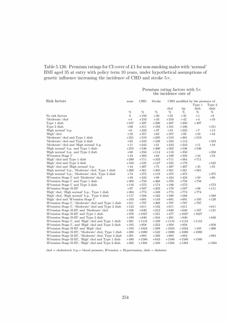
Table 5.126: Premium ratings for CI cover of £1 for non-smoking males with ‘normal’BMI aged 35 at entry with policy term 10 years, under hypothetical assumptions ofgenetic influence increasing the incidence of CHD and stroke 5×.
Premium rating factors with 5×the incidence rate of
Risk factors none CHD Stroke CHD modified by the presence ofType 1 Type 2
chol bp diab diab% % % % % % %
No risk factors 0 +192 +30 +32 +35 +1 +6‘Moderate’ chol +4 +210 +33 +210 +42 +4 +10Type 1 diab +247 +497 +290 +287 +292 +497Type 2 diab +60 +311 +103 +101 +106 +311‘High normal’ b.p. +6 +223 +37 +43 +223 +7 +13‘High’ chol +33 +357 +63 +357 +92 +34 +43‘Moderate’ chol and Type 1 diab +251 +519 +295 +519 +301 +519‘Moderate’ chol and Type 2 diab +65 +333 +108 +333 +114 +333‘Moderate’ chol and ‘High normal’ b.p. +11 +243 +41 +243 +243 +11 +18‘High normal’ b.p. and Type 1 diab +255 +536 +300 +302 +536 +536‘High normal’ b.p. and Type 2 diab +68 +350 +114 +116 +350 +350‘H’tension Stage I’ +43 +393 +82 +100 +393 +44 +53‘High’ chol and Type 1 diab +290 +711 +333 +711 +364 +711‘High’ chol and Type 2 diab +103 +525 +147 +525 +178 +525‘High’ chol and ‘High normal’ b.p. +44 +407 +75 +407 +407 +45 +55‘High normal’ b.p., ‘Moderate’ chol, Type 1 diab +260 +561 +305 +561 +561 +561‘High normal’ b.p., ‘Moderate’ chol, Type 2 diab +74 +375 +119 +375 +375 +375‘H’tension Stage I’ and ‘Moderate’ chol +49 +424 +89 +424 +424 +50 +60‘H’tension Stage I’ and Type 1 diab +303 +758 +360 +376 +758 +758‘H’tension Stage I’ and Type 2 diab +116 +572 +174 +190 +572 +572‘H’tension Stage II-III’ +97 +597 +203 +176 +597 +98 +111‘High’ chol, ‘High normal’ b.p., Type 1 diab +304 +774 +349 +774 +774 +774‘High’ chol, ‘High normal’ b.p., Type 2 diab +117 +588 +162 +588 +588 +588‘High’ chol and ‘H’tension Stage I’ +103 +691 +143 +691 +691 +105 +120‘H’tension Stage I’, ‘Moderate’ chol and Type 1 diab +311 +797 +369 +797 +797 +797‘H’tension Stage I’, ‘Moderate’ chol and Type 2 diab +124 +611 +182 +611 +611 +611‘H’tension Stage II-III’ and ‘Moderate’ chol +106 +640 +212 +640 +640 +107 +121‘H’tension Stage II-III’ and Type 1 diab +376 +1027 +531 +477 +1027 +1027‘H’tension Stage II-III’ and Type 2 diab +189 +840 +344 +291 +840 +840‘H’tension Stage I’, and ‘High’ chol and Type 1 diab +381 +1144 +439 +1144 +1144 +1144‘H’tension Stage I’, and ‘High’ chol and Type 2 diab +195 +958 +252 +958 +958 +958‘H’tension Stage II-III’ and ‘High’ chol +183 +1024 +289 +1024 +1024 +185 +206‘H’tension Stage II-III’, ‘Moderate’ chol, Type 1 diab +388 +1080 +542 +1080 +1080 +1080‘H’tension Stage II-III’, ‘Moderate’ chol, Type 2 diab +201 +894 +356 +894 +894 +894‘H’tension Stage II-III’, ‘High’ chol and Type 1 diab +489 +1580 +643 +1580 +1580 +1580‘H’tension Stage II-III’, ‘High’ chol and Type 2 diab +302 +1394 +456 +1394 +1394 +1394
chol = cholesterol, b.p.= blood pressure, H’tension = Hypertension, diab = diabetes
254

Table 5.127: Premium ratings for CI cover of £1 for non-smoking males with ‘normal’BMI aged 35 at entry with policy term 10 years, under hypothetical assumptions ofgenetic influence increasing the incidence of CHD and stroke 10×.
Premium rating factors with 10×the incidence rate of
Risk factors none CHD Stroke CHD modified by the presence ofType 1 Type 2
chol bp diab diab% % % % % % %
No risk factors 0 +432 +67 +70 +78 +1 +13‘Moderate’ chol +4 +465 +70 +465 +88 +5 +17Type 1 diab +247 +808 +344 +336 +345 +808Type 2 diab +60 +621 +158 +150 +159 +621‘High normal’ b.p. +6 +490 +76 +87 +490 +8 +21‘High’ chol +33 +758 +100 +758 +160 +35 +53‘Moderate’ chol and Type 1 diab +251 +850 +349 +850 +358 +850‘Moderate’ chol and Type 2 diab +65 +664 +162 +664 +173 +664‘Moderate’ chol and ‘High normal’ b.p. +11 +528 +80 +528 +528 +12 +26‘High normal’ b.p. and Type 1 diab +255 +881 +356 +357 +881 +881‘High normal’ b.p. and Type 2 diab +68 +695 +170 +171 +695 +695‘H’tension Stage I’ +43 +825 +132 +167 +825 +45 +65‘High’ chol and Type 1 diab +290 +1232 +387 +1232 +449 +1232‘High’ chol and Type 2 diab +103 +1045 +201 +1045 +263 +1045‘High’ chol and ‘High normal’ b.p. +44 +851 +113 +851 +851 +46 +67‘High normal’ b.p., ‘Moderate’ chol, Type 1 diab +260 +929 +362 +929 +929 +929‘High normal’ b.p., ‘Moderate’ chol, Type 2 diab +74 +743 +175 +743 +743 +743‘H’tension Stage I’ and ‘Moderate’ chol +49 +883 +138 +883 +883 +51 +73‘H’tension Stage I’ and Type 1 diab +303 +1317 +432 +458 +1317 +1317‘H’tension Stage I’ and Type 2 diab +116 +1131 +246 +273 +1131 +1131‘H’tension Stage II-III’ +97 +1214 +334 +265 +1214 +100 +126‘High’ chol, ‘High normal’ b.p., Type 1 diab +304 +1347 +405 +1347 +1347 +1347‘High’ chol, ‘High normal’ b.p., Type 2 diab +117 +1162 +218 +1162 +1162 +1162‘High’ chol and ‘H’tension Stage I’ +103 +1411 +192 +1411 +1411 +106 +137‘H’tension Stage I’, ‘Moderate’ chol and Type 1 diab +311 +1389 +440 +1389 +1389 +1389‘H’tension Stage I’, ‘Moderate’ chol and Type 2 diab +124 +1204 +254 +1204 +1204 +1204‘H’tension Stage II-III’ and ‘Moderate’ chol +106 +1292 +343 +1292 +1292 +109 +138‘H’tension Stage II-III’ and Type 1 diab +376 +1827 +723 +585 +1827 +1827‘H’tension Stage II-III’ and Type 2 diab +189 +1640 +537 +400 +1640 +1640‘H’tension Stage I’, and ‘High’ chol and Type 1 diab +381 +2074 +510 +2074 +2074 +2074‘H’tension Stage I’, and ‘High’ chol and Type 2 diab +195 +1888 +324 +1888 +1888 +1888‘H’tension Stage II-III’ and ‘High’ chol +183 +2052 +420 +2052 +2052 +187 +228‘H’tension Stage II-III’, ‘Moderate’ chol, Type 1 diab +388 +1922 +734 +1922 +1922 +1922‘H’tension Stage II-III’, ‘Moderate’ chol, Type 2 diab +201 +1736 +548 +1736 +1736 +1736‘H’tension Stage II-III’, ‘High’ chol and Type 1 diab +489 +2911 +834 +2911 +2911 +2911‘H’tension Stage II-III’, ‘High’ chol and Type 2 diab +302 +2725 +648 +2725 +2725 +2725
chol = cholesterol, b.p.= blood pressure, H’tension = Hypertension, diab = diabetes
255

Table 5.128: Premium ratings for CI cover of £1 for non-smoking males with ‘normal’BMI aged 35 at entry with policy term 10 years, under hypothetical assumptions ofgenetic influence increasing the incidence of CHD and stroke 20×.
Premium rating factors with 20×the incidence rate of
Risk factors none CHD Stroke CHD modified by the presence ofType 1 Type 2
chol bp diab diab% % % % % % %
No risk factors 0 +905 +140 +141 +156 +2 +25‘Moderate’ chol +4 +967 +144 +967 +173 +6 +30Type 1 diab +247 +1421 +452 +423 +442 +1421Type 2 diab +60 +1235 +266 +238 +257 +1235‘High normal’ b.p. +6 +1013 +152 +167 +1013 +9 +35‘High’ chol +33 +1548 +173 +1548 +280 +37 +72‘Moderate’ chol and Type 1 diab +251 +1498 +456 +1498 +462 +1498‘Moderate’ chol and Type 2 diab +65 +1313 +270 +1313 +277 +1313‘Moderate’ chol and ‘High normal’ b.p. +11 +1082 +157 +1082 +1082 +13 +41‘High normal’ b.p. and Type 1 diab +255 +1555 +468 +455 +1555 +1555‘High normal’ b.p. and Type 2 diab +68 +1369 +282 +270 +1369 +1369‘H’tension Stage I’ +43 +1671 +229 +283 +1671 +46 +84‘High’ chol and Type 1 diab +290 +2253 +495 +2253 +593 +2253‘High’ chol and Type 2 diab +103 +2067 +308 +2067 +409 +2067‘High’ chol and ‘High normal’ b.p. +44 +1712 +189 +1712 +1712 +48 +87‘High normal’ b.p., ‘Moderate’ chol, Type 1 diab +260 +1639 +473 +1639 +1639 +1639‘High normal’ b.p., ‘Moderate’ chol, Type 2 diab +74 +1455 +287 +1455 +1455 +1455‘H’tension Stage I’ and ‘Moderate’ chol +49 +1772 +236 +1772 +1772 +53 +94‘H’tension Stage I’ and Type 1 diab +303 +2407 +573 +598 +2407 +2407‘H’tension Stage I’ and Type 2 diab +116 +2221 +387 +413 +2221 +2221‘H’tension Stage II-III’ +97 +2422 +595 +414 +2422 +102 +151‘High’ chol, ‘High normal’ b.p., Type 1 diab +304 +2452 +516 +2452 +2452 +2452‘High’ chol, ‘High normal’ b.p., Type 2 diab +117 +2267 +330 +2267 +2267 +2267‘High’ chol and ‘H’tension Stage I’ +103 +2804 +289 +2804 +2804 +109 +164‘H’tension Stage I’, ‘Moderate’ chol and Type 1 diab +311 +2529 +581 +2529 +2529 +2529‘H’tension Stage I’, ‘Moderate’ chol and Type 2 diab +124 +2344 +395 +2344 +2344 +2344‘H’tension Stage II-III’ and ‘Moderate’ chol +106 +2554 +604 +2554 +2554 +111 +163‘H’tension Stage II-III’ and Type 1 diab +376 +3386 +1102 +759 +3386 +3386‘H’tension Stage II-III’ and Type 2 diab +189 +3200 +916 +575 +3200 +3200‘H’tension Stage I’, and ‘High’ chol and Type 1 diab +381 +3862 +650 +3862 +3862 +3862‘H’tension Stage I’, and ‘High’ chol and Type 2 diab +195 +3677 +464 +3677 +3677 +3677‘H’tension Stage II-III’ and ‘High’ chol +183 +4048 +680 +4048 +4048 +190 +259‘H’tension Stage II-III’, ‘Moderate’ chol, Type 1 diab +388 +3541 +1112 +3541 +3541 +3541‘H’tension Stage II-III’, ‘Moderate’ chol, Type 2 diab +201 +3356 +927 +3356 +3356 +3356‘H’tension Stage II-III’, ‘High’ chol and Type 1 diab +489 +5480 +1212 +5480 +5480 +5480‘H’tension Stage II-III’, ‘High’ chol and Type 2 diab +302 +5293 +1026 +5293 +5293 +5293
chol = cholesterol, b.p.= blood pressure, H’tension = Hypertension, diab = diabetes
256

Table 5.129: Premium ratings for CI cover of £1 for non-smoking males with ‘normal’BMI aged 35 at entry with policy term 10 years, under hypothetical assumptions ofgenetic influence increasing the incidence of CHD and stroke 50×.
Premium rating factors with 50×the incidence rate of
Risk factors none CHD Stroke CHD modified by the presence ofType 1 Type 2
chol bp diab diab% % % % % % %
No risk factors 0 +2288 +360 +317 +351 +5 +54‘Moderate’ chol +4 +2416 +364 +2416 +378 +9 +61Type 1 diab +247 +3206 +772 +631 +671 +3206Type 2 diab +60 +3020 +586 +446 +487 +3020‘High normal’ b.p. +6 +2506 +380 +359 +2506 +12 +67‘High’ chol +33 +3829 +393 +3829 +545 +40 +110‘Moderate’ chol and Type 1 diab +251 +3356 +776 +3356 +700 +3356‘Moderate’ chol and Type 2 diab +65 +3172 +591 +3172 +517 +3172‘Moderate’ chol and ‘High normal’ b.p. +11 +2641 +384 +2641 +2641 +16 +74‘High normal’ b.p. and Type 1 diab +255 +3462 +798 +677 +3462 +3462‘High normal’ b.p. and Type 2 diab +68 +3278 +613 +493 +3278 +3278‘H’tension Stage I’ +43 +4080 +514 +534 +4080 +50 +124‘High’ chol and Type 1 diab +290 +5188 +814 +5188 +889 +5188‘High’ chol and Type 2 diab +103 +5002 +629 +5002 +706 +5002‘High’ chol and ‘High normal’ b.p. +44 +4126 +417 +4126 +4126 +51 +127‘High normal’ b.p., ‘Moderate’ chol, Type 1 diab +260 +3618 +803 +3618 +3618 +3618‘High normal’ b.p., ‘Moderate’ chol, Type 2 diab +74 +3435 +618 +3435 +3435 +3435‘H’tension Stage I’ and ‘Moderate’ chol +49 +4261 +520 +4261 +4261 +57 +134‘H’tension Stage I’ and Type 1 diab +303 +5489 +979 +874 +5489 +5489‘H’tension Stage I’ and Type 2 diab +116 +5304 +795 +691 +5304 +5304‘H’tension Stage II-III’ +97 +5874 +1360 +701 +5874 +106 +193‘High’ chol, ‘High normal’ b.p., Type 1 diab +304 +5521 +846 +5521 +5521 +5521‘High’ chol, ‘High normal’ b.p., Type 2 diab +117 +5337 +660 +5337 +5337 +5337‘High’ chol and ‘H’tension Stage I’ +103 +6708 +572 +6708 +6708 +112 +207‘H’tension Stage I’, ‘Moderate’ chol and Type 1 diab +311 +5690 +987 +5690 +5690 +5690‘H’tension Stage I’, ‘Moderate’ chol and Type 2 diab +124 +5506 +803 +5506 +5506 +5506‘H’tension Stage II-III’ and ‘Moderate’ chol +106 +6088 +1368 +6088 +6088 +115 +206‘H’tension Stage II-III’ and Type 1 diab +376 +7818 +2203 +1061 +7818 +7818‘H’tension Stage II-III’ and Type 2 diab +189 +7630 +2020 +878 +7630 +7630‘H’tension Stage I’, and ‘High’ chol and Type 1 diab +381 +8851 +1055 +8851 +8851 +8851‘H’tension Stage I’, and ‘High’ chol and Type 2 diab +195 +8663 +870 +8663 +8663 +8663‘H’tension Stage II-III’ and ‘High’ chol +183 +9682 +1443 +9682 +9682 +194 +301‘H’tension Stage II-III’, ‘Moderate’ chol, Type 1 diab +388 +8050 +2213 +8050 +8050 +8050‘H’tension Stage II-III’, ‘Moderate’ chol, Type 2 diab +201 +7863 +2030 +7863 +7863 +7863‘H’tension Stage II-III’, ‘High’ chol and Type 1 diab +489 +12732 +2309 +12732 +12732 +12732‘H’tension Stage II-III’, ‘High’ chol and Type 2 diab +302 +12539 +2126 +12539 +12539 +12539
chol = cholesterol, b.p.= blood pressure, H’tension = Hypertension, diab = diabetes
257

Table 5.130: Premium ratings for CI cover of £1 for non-smoking males with ‘normal’BMI aged 35 at entry with policy term 30 years, under hypothetical assumptions ofgenetic influence increasing the incidence rate of CHD and stroke 5×.
Premium rating factors with 5×the incidence rate of
Risk factors none CHD Stroke CHD modified by the presence ofType 1 Type 2
chol bp diab diab% % % % % % %
No risk factors 0 +135 +34 +53 +63 +1 +14‘Moderate’ chol +5 +156 +39 +156 +76 +6 +21Type 1 diab +117 +283 +162 +178 +189 +283Type 2 diab +33 +201 +79 +96 +108 +201‘High normal’ b.p. +11 +172 +52 +75 +172 +12 +28‘High’ chol +21 +232 +55 +232 +112 +23 +41‘Moderate’ chol and Type 1 diab +123 +307 +168 +307 +204 +307‘Moderate’ chol and Type 2 diab +39 +226 +85 +226 +123 +226‘Moderate’ chol and ‘High normal’ b.p. +17 +197 +58 +197 +197 +19 +36‘High normal’ b.p. and Type 1 diab +130 +326 +183 +203 +326 +326‘High normal’ b.p. and Type 2 diab +46 +245 +101 +122 +245 +245‘H’tension Stage I’ +34 +263 +91 +117 +263 +36 +55‘High’ chol and Type 1 diab +143 +403 +188 +403 +247 +403‘High’ chol and Type 2 diab +60 +322 +105 +322 +166 +322‘High’ chol and ‘High normal’ b.p. +37 +284 +77 +284 +284 +39 +60‘High normal’ b.p., ‘Moderate’ chol, Type 1 diab +137 +354 +190 +354 +354 +354‘High normal’ b.p., ‘Moderate’ chol, Type 2 diab +54 +274 +108 +274 +274 +274‘H’tension Stage I’ and ‘Moderate’ chol +43 +295 +99 +295 +295 +45 +66‘H’tension Stage I’ and Type 1 diab +160 +441 +233 +254 +441 +441‘H’tension Stage I’ and Type 2 diab +77 +360 +152 +173 +360 +360‘H’tension Stage II-III’ +65 +363 +167 +163 +363 +68 +90‘High’ chol, ‘High normal’ b.p., Type 1 diab +162 +462 +213 +462 +462 +462‘High’ chol, ‘High normal’ b.p., Type 2 diab +79 +383 +132 +383 +383 +383‘High’ chol and ‘H’tension Stage I’ +72 +426 +126 +426 +426 +74 +100‘H’tension Stage I’, ‘Moderate’ chol and Type 1 diab +170 +477 +242 +477 +477 +477‘H’tension Stage I’, ‘Moderate’ chol and Type 2 diab +87 +397 +161 +397 +397 +397‘H’tension Stage II-III’ and ‘Moderate’ chol +76 +401 +176 +401 +401 +78 +102‘H’tension Stage II-III’ and Type 1 diab +201 +569 +335 +312 +569 +569‘H’tension Stage II-III’ and Type 2 diab +118 +489 +255 +232 +489 +489‘H’tension Stage I’, and ‘High’ chol and Type 1 diab +207 +642 +276 +642 +642 +642‘H’tension Stage I’, and ‘High’ chol and Type 2 diab +124 +562 +196 +562 +562 +562‘H’tension Stage II-III’ and ‘High’ chol +115 +580 +213 +580 +580 +117 +146‘H’tension Stage II-III’, ‘Moderate’ chol, Type 1 diab +213 +612 +346 +612 +612 +612‘H’tension Stage II-III’, ‘Moderate’ chol, Type 2 diab +131 +532 +266 +532 +532 +532‘H’tension Stage II-III’, ‘High’ chol and Type 1 diab +263 +842 +392 +842 +842 +842‘H’tension Stage II-III’, ‘High’ chol and Type 2 diab +180 +762 +312 +762 +762 +762
chol = cholesterol, b.p.= blood pressure, H’tension = Hypertension, diab = diabetes
258

known. Therefore for a life with similar other risk factors, no diabetes but with a
mutation associated with diabetes should have a rating not exceeding the one for a
life who already has diabetes. The significance of any mutation was seen to depend
on:
(a) the risk multiplier associated with the mutation,
(b) the term of policy, and
(c) age at entry.
The results showed a greater impact on ratings for mutations associated with
hypertension than with hypercholesterolaemia or diabetes.
Ratings based on hypothetical genetic influence which increased the direct inci-
dence of CHD were high even for moderate values of the risk multiplier. The ratings
associated with mutations for stroke were much less than those for CHD.
The ratings associated with higher direct incidence of CHD and stroke are much
higher than those associated with higher incidence of the risk factors. Comparing
ratings in Tables 5.125 and 5.122 shows that a risk multiplier of 2 for the direct
incidence rates will lead to generally higher ratings than a risk multiplier of 10 for
the indirect incidence rates. This indicates that genetic mutations which influence
the direct risk of CHD or stroke, or those which modify the influence of risk factors
on CHD incidence, are likely to have more impact on insurance costs than mutations
which increase the risk of onset of the risk factors.
5.4.2 Potential for adverse selection
The results we have considered so far are ratings for lives with specified risk factors
in particular subpopulations in relation to the premium payable by non-smoking
males with normal BMI. In practice ratings would be relative to a premium payable
by a broader group of lives. Also in practice the ratings, and overall underwriting,
are derived with consideration of the possibilities of anti-selection. Therefore to
give more conclusive assessments on insurability of lives we need to consider the
following:
(a) The relative sizes of the subpopulations and states within subpopulations. This
influences the level of the standard premium and also the impact of anti-selection
259
by lives in any of the states and subpopulations.
(b) The insurance buying behaviour of lives in the various states and subpopula-
tions.
To put this in context we note that for BCOC, in the absence of adverse selection,
mutation carriers could be insured at standard rates even with the high insurance
costs of mutation carriers shown in Table 3.48. We went on to conclude that under
modest forms of adverse selection, costs of insuring BRCA1 and BRCA2 mutation
carriers could be absorbed without large increases in the aggregate premiums. The
insurability, or not, of carriers of mutations associated with CHD and stroke depends
on the results of the interplay of factors in a model for adverse selection.
5.4.3 Ongoing assessment of the impact of genetic advances
on insurability
Our results on heart disease and stroke represent a first step to quantifying the
impact of genetics on insurance. We have shown that the insurance costs associated
with mutations that increase the risk of onset of risk factors can be significant. Even
more significant insurance costs are likely for mutations which have a direct impact
on CHD and stroke incidence. The insurance industry should regularly monitor
developments in the genetics of cardiovascular diseases and we feel any new results
can be fed into our model to assess the implications on insurance costs.
Using realistic assumptions and various models of anti-selection by mutation
carriers, our model can give indications on whether some mutation carriers can
be insured, with limits on sum assured values, as the case is for BCOC.
5.4.4 Application to insurance underwriting
The transition intensities used in the model are based on population based studies.
In Section 4.8.1 we showed that the model produces overall incidence rates of CHD
and stroke which are comparable with current population incidence rates. As it is
for permanent assurances in life insurance, we would expect the CI claim causes
experience for insured lives to be lighter than for the general population. In the
260
analysis of the CI claims experience for 1991–1997, Dinani et al. (2000) state that
they observe temporary initial selection but it was not possible to gauge the level of
the ultimate rates. This was due to little data being available at longer durations. A
crude approach to adjusting the population CI incidence rates in our model would
be to assume that morbidity differentials between insured lives and the general
population are the same as the mortality differentials. A more demanding approach
involves parameterising our model for each social-class. This requires more detailed
data than we had for this study. With social-class specific incidence rates, we can
then use assumptions about the social-class composition of the insured population,
which would be weighted in favour of the higher social classes in the population.
The model, without any genetic component, can then be used to construct an
underwriting manual or check ratings that are currently being used. We feel this
may be an important use with the advent of evidence based underwriting.
261

Chapter 6
Conclusions and further research
This thesis takes further the results of Macdonald (1997). We have considered CI as
a specific insurance product which insures against morbidity risk as opposed to mor-
tality. This work also considers the genetics of specific disorders. In Chapters 2 and
3 we assessed the impact of information about the known gene mutations associated
with breast and ovarian cancer. In Chapters 4 and 5 we looked at the importance
of information on hypothetical genes associated with heart disease, stroke and their
main risk factors hypertension, hypercholesterolaemia and diabetes. In both the
investigations for BCOC and for CHD and stroke, the assessment of the impact of
gene mutations was carried out within the framework of a completely specified CI
policy. This means that we took into account the background incidence of all the
main causes of CI claim, as well as mortality. We also took into account the risk
factors that are already used in the underwriting of lives for CI policies. This al-
lowed us to give more realistic results on the effect of genetic information on current
CI underwriting.
6.1 Breast and Ovarian Cancer
6.1.1 Conclusions
The basis of the BCOC work was the construction of a family history model specific
to the genotype of the applicant. This enabled us to calculate the carrier proba-
bilities associated with given family histories. The family histories represent the
262

information that may be available to insurance underwriters and the carrier proba-
bilities link this information to the genetic status of the applicant.
A model for CI insurance was also developed which took into account the inci-
dence of BCOC, other cancers, heart disease, stroke and other minor causes of CI
claims. Only BCOC incidences were assumed to depend on the genetic status at
BRCA1 and BRCA2.
Using the model for CI insurance and the results of the family history model, we
assessed the insurance costs associated with the gene mutations assuming that we
have:
(a) full information on the applicant’s relatives, their ages and their history of
BCOC, or
(b) partial or summarised information on relatives and their history of BCOC.
Full information is unlikely to be available at underwriting for CI policies.
Based on an adverse selection model which considers the rate of genetic testing
in the population and associated rates of insurance purchase, we managed to spec-
ify some conditions associated with the costs of adverse selection to the insurance
industry. If the high penetrance of BRCA1 and BRCA2 mutations associated with
members of some high risk families with mutations at these loci are applicable to
all mutation carriers then the costs of adverse selection may be significant. The
purchase of very high sums assured by mutation carriers and a small size for the CI
market also contribute to high costs of adverse selection. In the absence of these
conditions, it is unlikely that antiselection, based on the knowledge of genetic status
of BRCA1 and BRCA2, will result in substantial increases in the cost of insurance
for non-mutation carriers.
6.1.2 Contribution
We provide a family history model for the evaluation of carrier probabilities with the
family history defined in terms of categories used in insurance underwriting. This
gives the probability that an applicant for CI insurance is a mutation carrier using
family history information typically available to underwriters.
263

The work then quantifies the costs of CI insurance for individuals with and with-
out mutations at BRCA1 and BRCA2. These costs are derived based on incidence
rates of BCOC from studies of actual families with these mutations and from na-
tional statistics based on large population data sets. It establishes that the cost of
CI insurance for an individual with a BRCA1 or BRCA2 mutation is much higher
than the costs for lives without mutations even when the incidence of other main
CI claim causes like heart disease and stroke does not depend on genetic status.
We confirm that the results of Macdonald (1997) also apply to adverse selection
associated with the specific gene mutations BRCA1 and BRCA2 and CI insurance.
These results, stated in the previous section, are that adverse selection is unlikely
to cause a substantial increase to the insurance costs unless the market is small and
mutation carriers take out very high sums assured.
The thesis gives the level of change in insurance costs that is associated with
a fall in the penetrance estimates of BRCA1 and BRCA2 from the level initially
given in epidemiology publications. The effect of using different values for BRCA1
or BRCA2 mutation frequencies in the population is also quantified.
6.1.3 Further research
It was assumed that lives with BRCA1 mutations all have the same risk of BCOC
and that lives with BRCA2 have the same risk of BCOC. There is a need to assess
the extent to which the risk of BCOC in mutation carriers differs between members
of high risk families and those who are not from such families. The developments
in genetics regarding this heterogeneity of risk associated with different mutations
need to be monitored so that when this difference in risk has been quantified, we
can assess how the impact on insurance costs differ from our current results.
We need to extend the CI model to a life insurance model. We have stated before
that this requires the estimation of the incidence of death in lives with BCOC. The
incidence of deaths in these lives may depend more on the duration since onset of
disease than on the age of the life. We have identified the U.K. data available on
cancer registrations as ideal for such work.
264

Both the CI and possible life model will have been parameterised using population
data. The incidence of CI and of death in insured lives may be significantly different
than for the general population. It will be useful, mainly for purposes of using these
models as tools for pricing CI and life insurance, for the incidence rates of CI and
death to be adjusted to reflect the level in respect of the insured lives. The results
that come from the analysis of claims of policies that have already been sold may
be very useful in assessing the need and the possible level of any adjustment of
the population rates to apply to insured lives. We note that for the purposes of
deriving ratings only (differentials in risk between different groups of lives), the use
of population rates should be reasonably sufficient.
6.2 CHD and Stroke
6.2.1 Conclusions and contribution
Models for CHD and stroke in the literature take into account the initial profile of
risk factors. Given that they are parameterised from data from lives who moved
through various levels of the risk factors it means that these profiles implicitly take
into account progression through risk factors enroute to CHD or stroke. Our work
represents an advance on these models in that it explicitly models the intermediate
transitions through the risk factors. This was necessitated by the need to make
hypothetical assumptions about gene mutations acting on risk factors. Our model
produced remarkably similar results to models which do not model risk factors ex-
plicitly, with the added advantage of being able to assess the effect of changing the
incidence of one or more risk factors.
We applied our CHD and stroke model within a CI insurance context to produce
insurance costs and premium ratings associated with specific combinations of risk
factors. The ratings were in reasonable agreement with the underwriting guidelines
used in industry. Our feeling is that the model can have an important role in deriving
evidence based rating guidelines.
Due to the virtual unavailability of epidemiological genetics associated with CHD
and stroke we assumed hypothetical mutations existed which conferred extra CHD
265

and stroke risk in different ways. We concluded that mutations that increase risk
of CHD and stroke through risk factors are not likely to add much knowledge to
current underwriting. We also note that the impact on insurance costs of mutations
acting in this way is generally less than that of mutations which increase the direct
incidence of CHD and stroke.
The penetrance of mutations will strongly determine the insurance costs espe-
cially for the mutations that impact on direct CHD and stroke incidence. Assuming
that the insurability of an individual depends on their rating falling below +200,
mutations increasing the incidence of risk factors by up to 50 times more than in
non-mutation carriers rarely resulted in a change from acceptance to declinature.
However the actual changes in the ratings were significant.
We provided a model that can be used to calculate the effect of changes in the
incidence of any of the CHD and stroke risk factors on the incidence of the CHD and
stroke endpoints themselves. We used the model to assess the impact of genetics on
insurance but it can be used for a wide range of purposes like assessing the impact
of prevention of these risk factors on the burden from cardiovascular disorders to a
country’s health system.
6.2.2 Further research
We discussed the need to develop an adverse selection model to derive more infor-
mative results on the level of risk due to mutations that can be considered insurable.
This depends on the assumed frequencies of mutations. Our discussion on the genet-
ics of CHD and stroke point to the expectation of common, rather than rare, genes
being associated with quantitative traits like the risk factors. It is maybe that if the
mutation frequencies of any assumed mutations are high then even low penetrance
assumptions could lead to large changes to insurance costs for the whole insured
portfolio.
Therefore the development of an adverse selection model represents an important
area of further research. However it is also important that research is done to validate
the CHD and stroke models we have developed. Data from other epidemiological
studies can be used. However, ideally, data based on lives with CI policies should
266

be used to test the adequacy of the model for an insured population.
In this work it was appropriate to assume that the incidence of CHD and stroke
was dependent on the highest ever attained levels of blood pressure, cholesterol or
sugar. Should the current level of any of these risk factors be more informative than
the highest ever value, then we need to capture that in the modelling. This area
of possible future work requires modelling with allowance for reverse movements
between the risk factor states in Figures 4.29 and 5.47. The transition intensities
for the recoveries may depend more on duration of stay in the respective states than
on age at the time of recovery.
There is also a need to investigate the possibility of developing a family history
model along the lines of the BCOC model. This may be achieved by assuming
genotypes for an individual’s ancestors and using simulation techniques to generate
possible family structures down the generations. A distribution of family structures
could then be used with our model to produce family histories of risk factors, CHD
and stroke under some hypothetical genetic assumptions. The complications arising
from
(a) the presence of both males and females in the models, as compared to just
females in the BCOC model,
(b) the possibility of many genes interacting to influence heart disease, stroke and
the risk factors, and,
(c) the requirement to allow for environmental interactions
make the production of such a family history model a challenging task.
An extension of our model to a life insurance model is also an important future
research avenue. This requires the modelling of mortality after an CHD event or
stroke. This can be used to price the newer innovations on CI policies like the
buy-back facility.
267
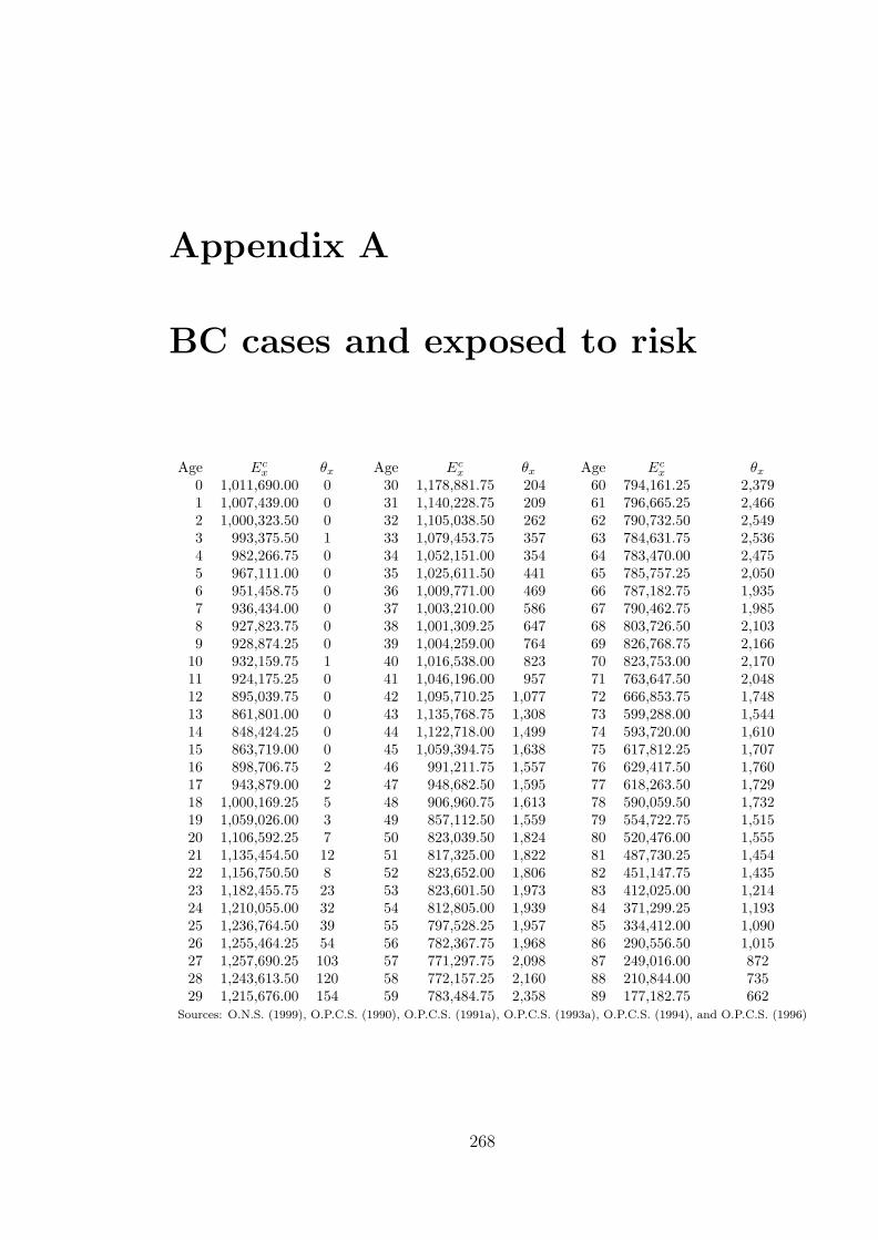
Appendix A
BC cases and exposed to risk
Age Ecx θx Age Ec
x θx Age Ecx θx
0 1,011,690.00 0 30 1,178,881.75 204 60 794,161.25 2,3791 1,007,439.00 0 31 1,140,228.75 209 61 796,665.25 2,4662 1,000,323.50 0 32 1,105,038.50 262 62 790,732.50 2,5493 993,375.50 1 33 1,079,453.75 357 63 784,631.75 2,5364 982,266.75 0 34 1,052,151.00 354 64 783,470.00 2,4755 967,111.00 0 35 1,025,611.50 441 65 785,757.25 2,0506 951,458.75 0 36 1,009,771.00 469 66 787,182.75 1,9357 936,434.00 0 37 1,003,210.00 586 67 790,462.75 1,9858 927,823.75 0 38 1,001,309.25 647 68 803,726.50 2,1039 928,874.25 0 39 1,004,259.00 764 69 826,768.75 2,166
10 932,159.75 1 40 1,016,538.00 823 70 823,753.00 2,17011 924,175.25 0 41 1,046,196.00 957 71 763,647.50 2,04812 895,039.75 0 42 1,095,710.25 1,077 72 666,853.75 1,74813 861,801.00 0 43 1,135,768.75 1,308 73 599,288.00 1,54414 848,424.25 0 44 1,122,718.00 1,499 74 593,720.00 1,61015 863,719.00 0 45 1,059,394.75 1,638 75 617,812.25 1,70716 898,706.75 2 46 991,211.75 1,557 76 629,417.50 1,76017 943,879.00 2 47 948,682.50 1,595 77 618,263.50 1,72918 1,000,169.25 5 48 906,960.75 1,613 78 590,059.50 1,73219 1,059,026.00 3 49 857,112.50 1,559 79 554,722.75 1,51520 1,106,592.25 7 50 823,039.50 1,824 80 520,476.00 1,55521 1,135,454.50 12 51 817,325.00 1,822 81 487,730.25 1,45422 1,156,750.50 8 52 823,652.00 1,806 82 451,147.75 1,43523 1,182,455.75 23 53 823,601.50 1,973 83 412,025.00 1,21424 1,210,055.00 32 54 812,805.00 1,939 84 371,299.25 1,19325 1,236,764.50 39 55 797,528.25 1,957 85 334,412.00 1,09026 1,255,464.25 54 56 782,367.75 1,968 86 290,556.50 1,01527 1,257,690.25 103 57 771,297.75 2,098 87 249,016.00 87228 1,243,613.50 120 58 772,157.25 2,160 88 210,844.00 73529 1,215,676.00 154 59 783,484.75 2,358 89 177,182.75 662
Sources: O.N.S. (1999), O.P.C.S. (1990), O.P.C.S. (1991a), O.P.C.S. (1993a), O.P.C.S. (1994), and O.P.C.S. (1996)
268
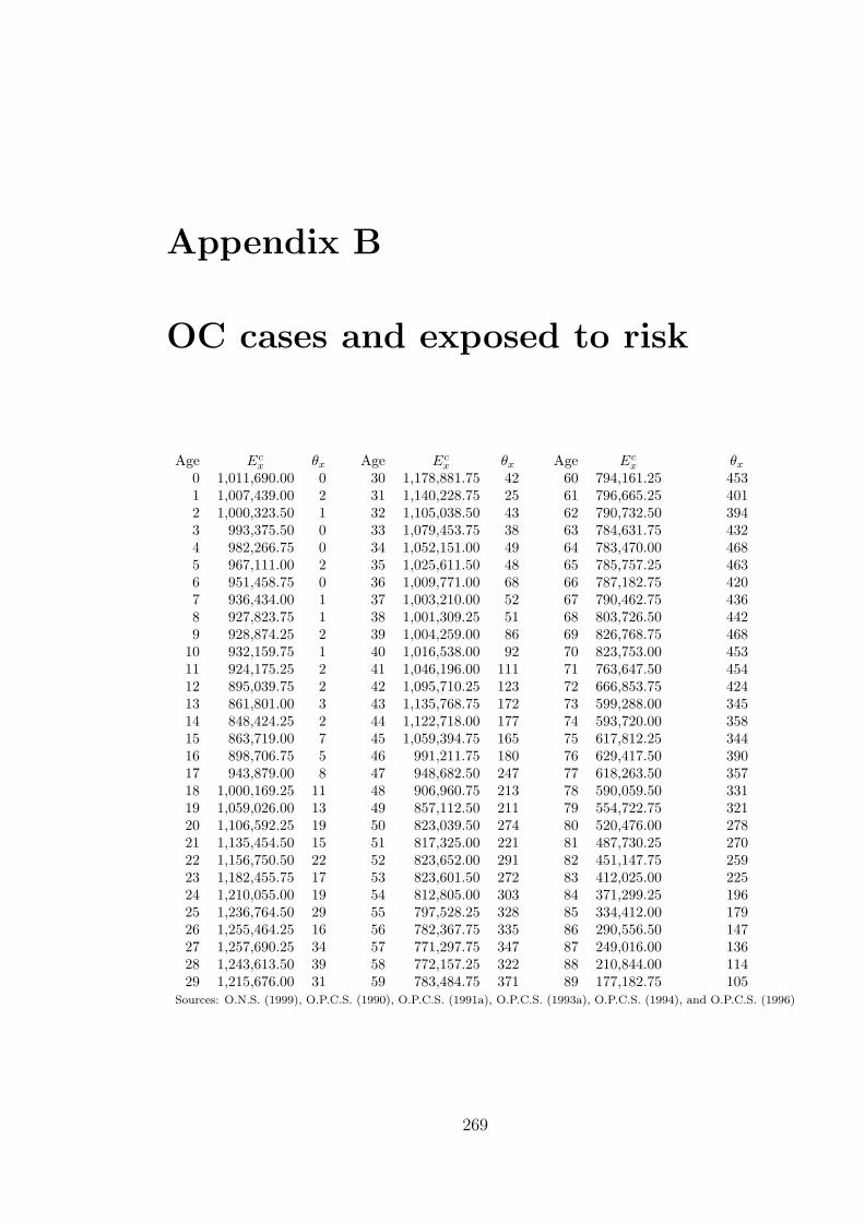
Appendix B
OC cases and exposed to risk
Age Ecx θx Age Ec
x θx Age Ecx θx
0 1,011,690.00 0 30 1,178,881.75 42 60 794,161.25 4531 1,007,439.00 2 31 1,140,228.75 25 61 796,665.25 4012 1,000,323.50 1 32 1,105,038.50 43 62 790,732.50 3943 993,375.50 0 33 1,079,453.75 38 63 784,631.75 4324 982,266.75 0 34 1,052,151.00 49 64 783,470.00 4685 967,111.00 2 35 1,025,611.50 48 65 785,757.25 4636 951,458.75 0 36 1,009,771.00 68 66 787,182.75 4207 936,434.00 1 37 1,003,210.00 52 67 790,462.75 4368 927,823.75 1 38 1,001,309.25 51 68 803,726.50 4429 928,874.25 2 39 1,004,259.00 86 69 826,768.75 468
10 932,159.75 1 40 1,016,538.00 92 70 823,753.00 45311 924,175.25 2 41 1,046,196.00 111 71 763,647.50 45412 895,039.75 2 42 1,095,710.25 123 72 666,853.75 42413 861,801.00 3 43 1,135,768.75 172 73 599,288.00 34514 848,424.25 2 44 1,122,718.00 177 74 593,720.00 35815 863,719.00 7 45 1,059,394.75 165 75 617,812.25 34416 898,706.75 5 46 991,211.75 180 76 629,417.50 39017 943,879.00 8 47 948,682.50 247 77 618,263.50 35718 1,000,169.25 11 48 906,960.75 213 78 590,059.50 33119 1,059,026.00 13 49 857,112.50 211 79 554,722.75 32120 1,106,592.25 19 50 823,039.50 274 80 520,476.00 27821 1,135,454.50 15 51 817,325.00 221 81 487,730.25 27022 1,156,750.50 22 52 823,652.00 291 82 451,147.75 25923 1,182,455.75 17 53 823,601.50 272 83 412,025.00 22524 1,210,055.00 19 54 812,805.00 303 84 371,299.25 19625 1,236,764.50 29 55 797,528.25 328 85 334,412.00 17926 1,255,464.25 16 56 782,367.75 335 86 290,556.50 14727 1,257,690.25 34 57 771,297.75 347 87 249,016.00 13628 1,243,613.50 39 58 772,157.25 322 88 210,844.00 11429 1,215,676.00 31 59 783,484.75 371 89 177,182.75 105
Sources: O.N.S. (1999), O.P.C.S. (1990), O.P.C.S. (1991a), O.P.C.S. (1993a), O.P.C.S. (1994), and O.P.C.S. (1996)
269

Appendix C
Mortality adjustment data set
Age Deaths Age Deaths Age DeathsTotal BC OC Total BC OC Total BC OC
1 555 0 0 33 597 91 15 65 11,195 958 3632 300 0 0 34 659 77 15 66 11,951 893 3283 227 0 0 35 724 103 13 67 13,422 972 3654 178 0 0 36 750 116 18 68 14,871 989 3655 138 0 1 37 829 121 21 69 16,827 1,116 3766 151 0 0 38 883 166 26 70 18,832 1,152 3927 129 0 0 39 1,004 170 36 71 18,529 1,025 3818 125 0 0 40 1,067 206 32 72 18,199 951 3599 139 0 0 41 1,201 257 31 73 17,820 808 348
10 113 0 0 42 1,490 307 54 74 19,703 954 29811 132 0 0 43 1,536 313 73 75 22,735 952 29612 127 0 0 44 1,811 387 87 76 25,340 973 31313 108 0 0 45 1,908 425 92 77 27,799 1,070 32514 171 0 0 46 1,935 405 93 78 29,187 1,063 31215 187 0 1 47 2,087 454 102 79 30,590 1,039 28016 232 0 2 48 2,217 458 112 80 32,073 1,050 24917 308 0 3 49 2,203 456 113 81 33,378 1,092 26218 297 0 0 50 2,412 471 151 82 34,440 1,027 23819 342 0 3 51 2,650 529 160 83 34,924 945 20720 340 1 1 52 3,000 561 166 84 34,790 950 18721 377 1 3 53 3,200 611 182 85 34,326 867 16422 384 1 0 54 3,430 638 175 86 33,617 803 14023 382 0 5 55 3,823 663 201 87 32,018 730 12324 392 3 4 56 4,134 661 214 88 29,331 616 11425 412 8 2 57 4,597 634 248 89 26,944 542 11226 441 7 6 58 5,043 690 235 90 24,454 493 6327 436 10 4 59 5,780 753 276 91 21,315 425 4528 498 32 10 60 6,661 804 301 92 18,206 316 4329 479 28 8 61 7,485 845 319 93 14,956 295 2630 473 38 6 62 7,989 787 297 94 12,102 202 1831 541 49 12 63 8,827 883 310 95 9,781 155 1832 617 57 12 64 10,060 901 333 96 7,476 131 6
Sources: O.P.C.S. (1991b), O.P.C.S. (1993b), O.P.C.S. (1993c) and O.N.S. (1997a).
270
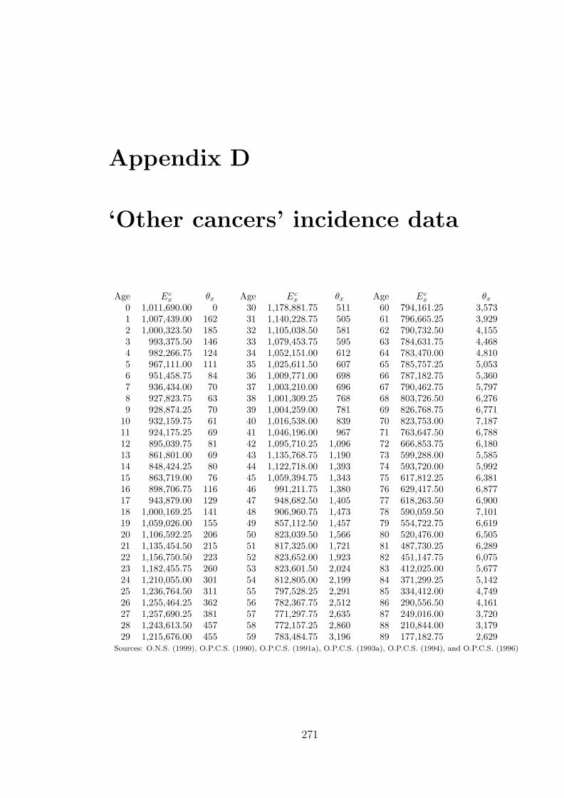
Appendix D
‘Other cancers’ incidence data
Age Ecx θx Age Ec
x θx Age Ecx θx
0 1,011,690.00 0 30 1,178,881.75 511 60 794,161.25 3,5731 1,007,439.00 162 31 1,140,228.75 505 61 796,665.25 3,9292 1,000,323.50 185 32 1,105,038.50 581 62 790,732.50 4,1553 993,375.50 146 33 1,079,453.75 595 63 784,631.75 4,4684 982,266.75 124 34 1,052,151.00 612 64 783,470.00 4,8105 967,111.00 111 35 1,025,611.50 607 65 785,757.25 5,0536 951,458.75 84 36 1,009,771.00 698 66 787,182.75 5,3607 936,434.00 70 37 1,003,210.00 696 67 790,462.75 5,7978 927,823.75 63 38 1,001,309.25 768 68 803,726.50 6,2769 928,874.25 70 39 1,004,259.00 781 69 826,768.75 6,771
10 932,159.75 61 40 1,016,538.00 839 70 823,753.00 7,18711 924,175.25 69 41 1,046,196.00 967 71 763,647.50 6,78812 895,039.75 81 42 1,095,710.25 1,096 72 666,853.75 6,18013 861,801.00 69 43 1,135,768.75 1,190 73 599,288.00 5,58514 848,424.25 80 44 1,122,718.00 1,393 74 593,720.00 5,99215 863,719.00 76 45 1,059,394.75 1,343 75 617,812.25 6,38116 898,706.75 116 46 991,211.75 1,380 76 629,417.50 6,87717 943,879.00 129 47 948,682.50 1,405 77 618,263.50 6,90018 1,000,169.25 141 48 906,960.75 1,473 78 590,059.50 7,10119 1,059,026.00 155 49 857,112.50 1,457 79 554,722.75 6,61920 1,106,592.25 206 50 823,039.50 1,566 80 520,476.00 6,50521 1,135,454.50 215 51 817,325.00 1,721 81 487,730.25 6,28922 1,156,750.50 223 52 823,652.00 1,923 82 451,147.75 6,07523 1,182,455.75 260 53 823,601.50 2,024 83 412,025.00 5,67724 1,210,055.00 301 54 812,805.00 2,199 84 371,299.25 5,14225 1,236,764.50 311 55 797,528.25 2,291 85 334,412.00 4,74926 1,255,464.25 362 56 782,367.75 2,512 86 290,556.50 4,16127 1,257,690.25 381 57 771,297.75 2,635 87 249,016.00 3,72028 1,243,613.50 457 58 772,157.25 2,860 88 210,844.00 3,17929 1,215,676.00 455 59 783,484.75 3,196 89 177,182.75 2,629
Sources: O.N.S. (1999), O.P.C.S. (1990), O.P.C.S. (1991a), O.P.C.S. (1993a), O.P.C.S. (1994), and O.P.C.S. (1996)
271

Appendix E
Cancer incidence data: Females
Age Ecx θL
x θOx Age Ec
x θLx θO
x Age Ecx θL
x θOx
0 1,011,690.00 1 136 30 1,178,881.75 8 506 60 794,161.25 715 3,4021 1,007,439.00 1 162 31 1,140,228.75 7 493 61 796,665.25 797 3,7132 1,000,323.50 1 184 32 1,105,038.50 11 573 62 790,732.50 880 3,9293 993,375.50 0 143 33 1,079,453.75 9 580 63 784,631.75 1,057 4,2624 982,266.75 0 123 34 1,052,151.00 16 600 64 783,470.00 1,165 4,5625 967,111.00 0 111 35 1,025,611.50 12 591 65 785,757.25 1,176 4,7916 951,458.75 0 84 36 1,009,771.00 20 688 66 787,182.75 1,300 5,1037 936,434.00 0 70 37 1,003,210.00 27 684 67 790,462.75 1,379 5,4558 927,823.75 0 63 38 1,001,309.25 34 746 68 803,726.50 1,436 5,9629 928,874.25 0 69 39 1,004,259.00 39 755 69 826,768.75 1,511 6,423
10 932,159.75 0 61 40 1,016,538.00 52 806 70 823,753.00 1,589 6,80711 924,175.25 0 69 41 1,046,196.00 61 935 71 763,647.50 1,495 6,45212 895,039.75 0 81 42 1,095,710.25 111 1,052 72 666,853.75 1,326 5,82313 861,801.00 0 68 43 1,135,768.75 95 1,129 73 599,288.00 1,202 5,27814 848,424.25 0 79 44 1,122,718.00 123 1,334 74 593,720.00 1,226 5,65415 863,719.00 1 75 45 1,059,394.75 133 1,284 75 617,812.25 1,260 5,99516 898,706.75 1 115 46 991,211.75 149 1,316 76 629,417.50 1,304 6,49617 943,879.00 4 129 47 948,682.50 203 1,349 77 618,263.50 1,252 6,50118 1,000,169.25 1 140 48 906,960.75 180 1,402 78 590,059.50 1,239 6,64219 1,059,026.00 0 153 49 857,112.50 207 1,397 79 554,722.75 1,024 6,16620 1,106,592.25 1 204 50 823,039.50 222 1,491 80 520,476.00 1,009 6,09321 1,135,454.50 1 208 51 817,325.00 237 1,656 81 487,730.25 972 5,88122 1,156,750.50 1 222 52 823,652.00 289 1,838 82 451,147.75 863 5,69423 1,182,455.75 3 258 53 823,601.50 296 1,931 83 412,025.00 750 5,31124 1,210,055.00 6 297 54 812,805.00 326 2,115 84 371,299.25 657 4,77825 1,236,764.50 4 307 55 797,528.25 321 2,195 85 334,412.00 522 4,41426 1,255,464.25 3 357 56 782,367.75 382 2,400 86 290,556.50 454 3,87427 1,257,690.25 0 375 57 771,297.75 460 2,523 87 249,016.00 408 3,42628 1,243,613.50 3 451 58 772,157.25 482 2,736 88 210,844.00 290 2,95729 1,215,676.00 6 450 59 783,484.75 602 3,039 89 177,182.75 235 2,426
θLx is Lung cancer exposed to risk θO
x is ‘Other’ cancers exposed to riskSources: O.N.S. (1999),O.P.C.S. (1990), O.P.C.S. (1991a), O.P.C.S. (1993a), O.P.C.S. (1994), and O.P.C.S. (1996)
272
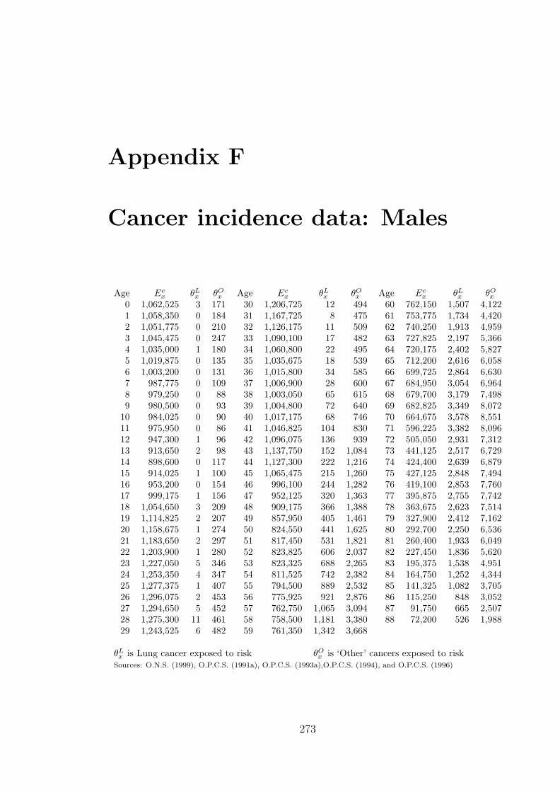
Appendix F
Cancer incidence data: Males
Age Ecx θL
x θOx Age Ec
x θLx θO
x Age Ecx θL
x θOx
0 1,062,525 3 171 30 1,206,725 12 494 60 762,150 1,507 4,1221 1,058,350 0 184 31 1,167,725 8 475 61 753,775 1,734 4,4202 1,051,775 0 210 32 1,126,175 11 509 62 740,250 1,913 4,9593 1,045,475 0 247 33 1,090,100 17 482 63 727,825 2,197 5,3664 1,035,000 1 180 34 1,060,800 22 495 64 720,175 2,402 5,8275 1,019,875 0 135 35 1,035,675 18 539 65 712,200 2,616 6,0586 1,003,200 0 131 36 1,015,800 34 585 66 699,725 2,864 6,6307 987,775 0 109 37 1,006,900 28 600 67 684,950 3,054 6,9648 979,250 0 88 38 1,003,050 65 615 68 679,700 3,179 7,4989 980,500 0 93 39 1,004,800 72 640 69 682,825 3,349 8,072
10 984,025 0 90 40 1,017,175 68 746 70 664,675 3,578 8,55111 975,950 0 86 41 1,046,825 104 830 71 596,225 3,382 8,09612 947,300 1 96 42 1,096,075 136 939 72 505,050 2,931 7,31213 913,650 2 98 43 1,137,750 152 1,084 73 441,125 2,517 6,72914 898,600 0 117 44 1,127,300 222 1,216 74 424,400 2,639 6,87915 914,025 1 100 45 1,065,475 215 1,260 75 427,125 2,848 7,49416 953,200 0 154 46 996,100 244 1,282 76 419,100 2,853 7,76017 999,175 1 156 47 952,125 320 1,363 77 395,875 2,755 7,74218 1,054,650 3 209 48 909,175 366 1,388 78 363,675 2,623 7,51419 1,114,825 2 207 49 857,950 405 1,461 79 327,900 2,412 7,16220 1,158,675 1 274 50 824,550 441 1,625 80 292,700 2,250 6,53621 1,183,650 2 297 51 817,450 531 1,821 81 260,400 1,933 6,04922 1,203,900 1 280 52 823,825 606 2,037 82 227,450 1,836 5,62023 1,227,050 5 346 53 823,325 688 2,265 83 195,375 1,538 4,95124 1,253,350 4 347 54 811,525 742 2,382 84 164,750 1,252 4,34425 1,277,375 1 407 55 794,500 889 2,532 85 141,325 1,082 3,70526 1,296,075 2 453 56 775,925 921 2,876 86 115,250 848 3,05227 1,294,650 5 452 57 762,750 1,065 3,094 87 91,750 665 2,50728 1,275,300 11 461 58 758,500 1,181 3,380 88 72,200 526 1,98829 1,243,525 6 482 59 761,350 1,342 3,668
θLx is Lung cancer exposed to risk θO
x is ‘Other’ cancers exposed to riskSources: O.N.S. (1999), O.P.C.S. (1991a), O.P.C.S. (1993a),O.P.C.S. (1994), and O.P.C.S. (1996)
273

Appendix G
Mortality adjustment factors
To derive the appropriate mortality rates we adjust ELT15M or ELT15F using
equation (2.16). The crude adjustment factors are given by
φx =θD
x
θELT15x
where θDx is the number of deaths, for lives aged x, in the ELT15 data which are
due to CHD or stroke as appropriate. θELT15x is the total number of deaths for lives
aged x in the ELT15 data. The total number of deaths θELT15x are given by O.N.S.
(1997a) but the number of deaths due to CHD or stroke, θDx , is approximated using
the mortality statistics O.P.C.S. (1991b), O.P.C.S. (1993b), O.P.C.S. (1993c) for the
years 1990 to 1992. The data is shown in Tables G.131. The data is aggregated in
mostly five year age groups since the data from O.P.C.S. (1991b), O.P.C.S. (1993b),
O.P.C.S. (1993c) is aggregated in this way. The adjustment factors were smoothed,
using unweighted least squares, by the following functions:
For males:
φCHD(x) =
exp(−9.4142 + 0.2008× x) : x ≤ 32.5
−1.479 + 7.400× 10⁻² × x− 9.478× 10⁻⁴ × x2 + 3.734× 10⁻⁶ × x3 : x ≥ 38
with linear blending for 32.5 < x < 38,
φSTR(x) = 0.2274− 3.079× 10⁻² × x + 1.555× 10⁻³ × x2 − 3.478× 10⁻⁵ × x3
+3.602× 10⁻⁷ × x4 − 1.392× 10⁻⁹ × x5
for x ≥ 20, and 0 otherwise.
274

For females:
φCHD(x) = exp(−9.201 + 2.057× 10⁻¹ × x− 1.337× 10⁻³ × x2),
and
φSTR(x) = 0.3306− 4.385× 10⁻² × x + 2.310× 10⁻³ × x2
−5.439× 10⁻⁵ × x3 + 5.878× 10⁻⁷ × x4 − 2.341× 10⁻⁹ × x5
for x ≥ 20, and 0 otherwise.
Figure G.57 shows, for ages 30 to 85, the crude mortality adjustment factors
together with the smoothed adjustment factors as given by the equations above.
Males: CHD.
Age
Mor
talit
y ad
just
men
t fac
tor
30 40 50 60 70 80
0.0
0.1
0.2
0.3
Males: Stroke.
Age
Mor
talit
y ad
just
men
t fac
tor
30 40 50 60 70 80
0.0
0.04
0.08
0.12
Females: CHD.
Age
Mor
talit
y ad
just
men
t fac
tor
30 40 50 60 70 80
0.0
0.10
0.20
0.30
Females: Stroke.
Age
Mor
talit
y ad
just
men
t fac
tor
30 40 50 60 70 80
0.0
0.05
0.10
0.15
0.20
Figure G.57: Crude and smoothed mortality adjustment factors.
275

Table G.131: Mortality adjustment data for CHD and stroke.
(Sources: O.P.C.S. (1991b), O.P.C.S. (1993b), O.P.C.S. (1993c) and O.N.S. (1997a).)
Age range Middle age Total deaths CHD deaths Stroke deaths
Males1 – 4 2.5 1,634 4 45 – 9 7 976 1 10
10 – 14 12 1,014 1 1015 – 19 17 3,472 5 2820 – 24 22 5,270 20 5325 – 29 27 5,542 103 8630 – 34 32 5,610 289 15435 – 39 37 7,104 973 22540 – 44 42 11,068 2,517 44745 – 49 47 15,860 4,728 74550 – 54 52 23,915 8,103 1,02655 – 59 57 38,889 13,990 1,91460 – 64 62 66,043 23,340 3,60665 – 69 67 105,365 35,987 6,56170 – 74 72 125,823 41,545 9,81575 – 79 77 148,932 45,303 14,37980 – 84 82 135,084 37,165 14,71685 – 89 87 80,844 19,878 8,97090 – 94 92 28,624 6,168 3,048
Females1 – 4 2.5 1,260 1 85 – 9 7 682 0 12
10 – 14 12 651 2 815 – 19 17 1,366 3 3220 – 24 22 1,875 7 5825 – 29 27 2,266 19 8730 – 34 32 2,887 70 13935 – 39 37 4,190 160 22940 – 44 42 7,105 408 42045 – 49 47 10,350 812 59450 – 54 52 14,692 1,660 85555 – 59 57 23,377 3,738 1,44160 – 64 62 41,022 8,588 2,79665 – 69 67 68,266 16,583 6,00270 – 74 72 93,083 25,210 10,87675 – 79 77 135,651 37,268 20,62280 – 84 82 169,605 44,518 30,37485 – 89 87 156,236 37,274 29,63290 – 94 92 91,033 18,836 16,566
276

Appendix H
Cardiovascular risk profiles
We define tpCHD[x] as the probability of a myocardial infarction event within t years
of a baseline examination taking place at age x. Taking
(a) sbp as the level of systolic blood pressure,
(b) chol as the ratio of total cholesterol to HDL-cholesterol levels,
(c) diab as 0 for non-diabetics and 1 for diabetics,
(d) smoking as 0 for non-smokers and 1 for smokers,
Anderson et al. (1991a) give,
tpCHD[x] = 1− exp
(−exp
[log(t)− a
exp(3.4064− 0.8584× a)
])(H.52)
where for males:
a = 11.4712− 0.7965× log(x)− 0.6623× log(sbp)− 0.2675× (smoking)
−0.4277× log(chol)− 0.1534× (diab)
and for females:
a = 21.9821− 6.2181× log(x) + 0.7101(log(x))2 − 0.6623× log(sbp)
−0.2675× (smoking)− 0.4277× log(chol)− 0.2699× (diab).
The probability of a stroke (STR) within t years of a baseline examination is given
by
277
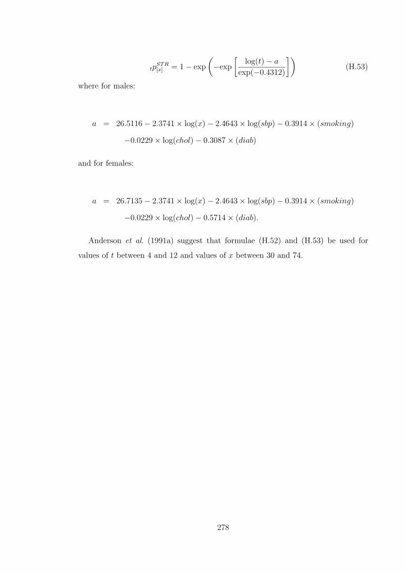
tpSTR[x] = 1− exp
(−exp
[log(t)− a
exp(−0.4312)
])(H.53)
where for males:
a = 26.5116− 2.3741× log(x)− 2.4643× log(sbp)− 0.3914× (smoking)
−0.0229× log(chol)− 0.3087× (diab)
and for females:
a = 26.7135− 2.3741× log(x)− 2.4643× log(sbp)− 0.3914× (smoking)
−0.0229× log(chol)− 0.5714× (diab).
Anderson et al. (1991a) suggest that formulae (H.52) and (H.53) be used for
values of t between 4 and 12 and values of x between 30 and 74.
278

Appendix I
Variance-covariance matrices
Table I.132: Variance-covariance matrices for fitting blood pressure incidence anddiabetes incidence.
Blood Pressure
Incidence of ‘High normal’ blood pressureα β ν
α 9.973× 10⁻² −1.636× 10⁻³ −4.420× 10⁻⁴
β 2.737× 10⁻⁵ 8.327× 10⁻⁶
ν 1.974× 10⁻³
Incidence of ‘Hypertension Stage I’α β γ
α 7.388× 10⁻² −1.165× 10⁻³ 8.039× 10⁻⁴
β 1.876× 10⁻⁵ −5.519× 10⁻⁶
γ 1.483× 10⁻³
Incidence of ‘Hypertension Stage II/III’α β γ
α 7.380× 10⁻² −1.130× 10⁻³ −3.854× 10⁻⁴
β 1.762× 10⁻⁵ 1.064× 10⁻⁵
γ 1.323× 10⁻³
Diabetes
α β να 1.085× 10⁻¹ −1.592× 10⁻³ −8.283× 10⁻⁴
β 2.375× 10⁻⁵ 6.645× 10⁻⁷
ν 1.876× 10⁻³
279

Table I.133: Variance-covariance matrices for fitting MI and stroke incidence.
MI fitting: Malesα δ0 δ1 η ρ φ β
α 1.274× 10⁻¹ −2.032× 10⁻³ −8.988× 10⁻⁴ 7.898× 10⁻⁴ 4.425× 10⁻³ −6.369× 10⁻³ −1.930× 10⁻³
δ0 8.164× 10⁻³ −4.501× 10⁻³ −3.348× 10⁻⁴ 2.082× 10⁻⁴ −3.032× 10⁻⁴ 6.327× 10⁻⁵
δ1 5.728× 10⁻³ 6.111× 10⁻⁵ −8.741× 10⁻⁵ −4.824× 10⁻⁵ 9.747× 10⁻⁶
η 3.622× 10⁻³ 1.664× 10⁻⁵ −2.047× 10⁻⁵ 1.832× 10⁻⁵
ρ 2.675× 10⁻³ 6.149× 10⁻⁵ −6.377× 10⁻⁵
φ 3.830× 10⁻³ 6.493× 10⁻⁵
β 3.057× 10⁻⁵
MI fitting: Femalesα δ0 δ1 β0 ρ φ η β1
α 14.32 −9.287× 10⁻² 3.736× 10⁻² −4.422× 10⁻¹ 2.774× 10⁻³ −8.008× 10⁻³ −3.879× 10⁻² 3.350× 10⁻³
δ0 3.355× 10⁻² −1.886× 10⁻² 2.855× 10⁻³ 5.216× 10⁻⁴ −2.889× 10⁻⁴ −2.932× 10⁻⁴ −1.914× 10⁻⁵
δ1 1.910× 10⁻² −1.202× 10⁻³ −1.288× 10⁻⁴ −1.746× 10⁻⁴ 3.673× 10⁻⁴ 9.030× 10⁻⁶
β0 1.378× 10⁻² 7.033× 10⁻⁵ −8.768× 10⁻⁵ 1.351× 10⁻³ −1.052× 10⁻⁴
ρ 6.831× 10⁻³ 1.125× 10⁻⁴ −6.519× 10⁻⁵ −2.127× 10⁻⁶
φ 8.246× 10⁻³ −9.597× 10⁻⁵ 2.055× 10⁻⁶
η 1.399× 10⁻² −8.987× 10⁻⁶
β1 8.094× 10⁻⁷
Stroke fittingα δ β ρ φ γ ψ
α 2.225× 10⁻¹ −5.174× 10⁻³ −3.266× 10⁻³ 6.265× 10⁻³ −8.298× 10⁻³ 1.793× 10⁻² −2.416× 10⁻⁴
δ 4.490× 10⁻³ 1.089× 10⁻⁴ 1.400× 10⁻⁴ −2.596× 10⁻⁴ 2.181× 10⁻³ −3.434× 10⁻⁵
β 4.916× 10⁻⁵ −1.029× 10⁻⁴ 8.790× 10⁻⁵ −2.516× 10⁻⁴ 3.328× 10⁻⁶
ρ 3.960× 10⁻³ 3.452× 10⁻⁵ 5.250× 10⁻⁴ 8.435× 10⁻⁶
φ 4.636× 10⁻³ 3.914× 10⁻⁴ −1.205× 10⁻⁶
γ 1.910× 10⁻¹ −2.805× 10⁻³
ψ 4.199× 10⁻⁵
280
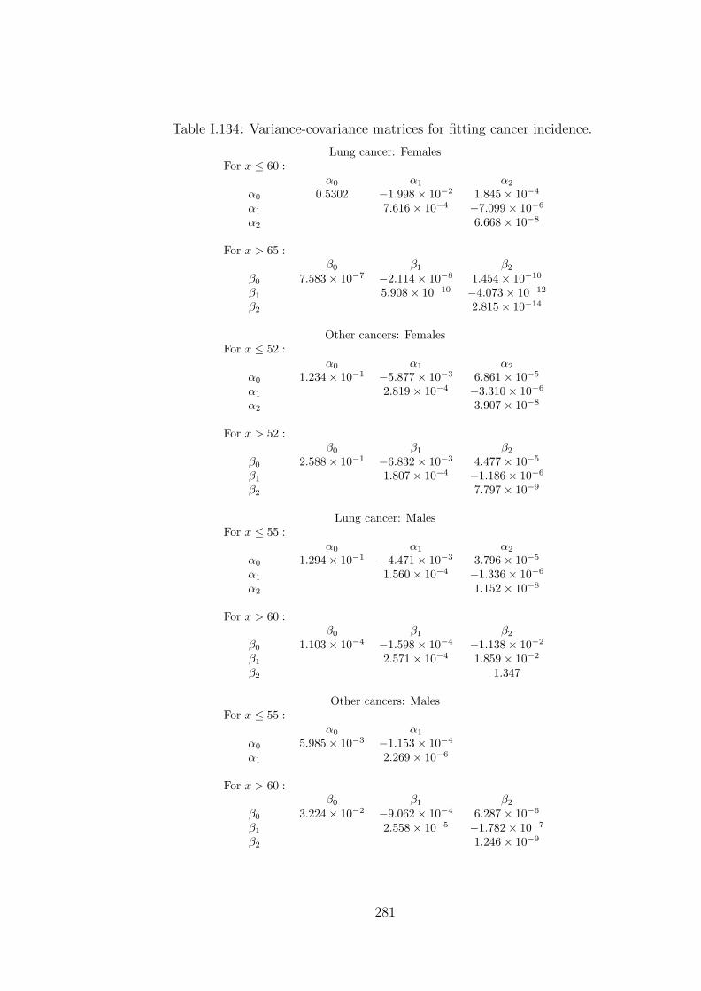
Table I.134: Variance-covariance matrices for fitting cancer incidence.
Lung cancer: FemalesFor x ≤ 60 :
α0 α1 α2
α0 0.5302 −1.998× 10⁻² 1.845× 10⁻⁴
α1 7.616× 10⁻⁴ −7.099× 10⁻⁶
α2 6.668× 10⁻⁸
For x > 65 :β0 β1 β2
β0 7.583× 10⁻⁷ −2.114× 10⁻⁸ 1.454× 10⁻¹⁰
β1 5.908× 10⁻¹⁰ −4.073× 10⁻¹²
β2 2.815× 10⁻¹⁴
Other cancers: FemalesFor x ≤ 52 :
α0 α1 α2
α0 1.234× 10⁻¹ −5.877× 10⁻³ 6.861× 10⁻⁵
α1 2.819× 10⁻⁴ −3.310× 10⁻⁶
α2 3.907× 10⁻⁸
For x > 52 :β0 β1 β2
β0 2.588× 10⁻¹ −6.832× 10⁻³ 4.477× 10⁻⁵
β1 1.807× 10⁻⁴ −1.186× 10⁻⁶
β2 7.797× 10⁻⁹
Lung cancer: MalesFor x ≤ 55 :
α0 α1 α2
α0 1.294× 10⁻¹ −4.471× 10⁻³ 3.796× 10⁻⁵
α1 1.560× 10⁻⁴ −1.336× 10⁻⁶
α2 1.152× 10⁻⁸
For x > 60 :β0 β1 β2
β0 1.103× 10⁻⁴ −1.598× 10⁻⁴ −1.138× 10⁻²
β1 2.571× 10⁻⁴ 1.859× 10⁻²
β2 1.347
Other cancers: MalesFor x ≤ 55 :
α0 α1
α0 5.985× 10⁻³ −1.153× 10⁻⁴
α1 2.269× 10⁻⁶
For x > 60 :β0 β1 β2
β0 3.224× 10⁻² −9.062× 10⁻⁴ 6.287× 10⁻⁶
β1 2.558× 10⁻⁵ −1.782× 10⁻⁷
β2 1.246× 10⁻⁹
281

Table I.135: Variance-covariance matrices for fitting kidney failure incidence.
MalesNon-diabetic
α0 α1
α0 2.471× 10⁻² −3.415× 10⁻⁴
α1 4.768× 10⁻⁶
Type 1 diabeticsα0 α1 α2 α3
α0 1.255 −7.660× 10⁻² 1.484× 10⁻³ −9.198× 10⁻⁶
α1 4.707× 10⁻³ −9.172× 10⁻⁵ 5.718× 10⁻⁷
α2 1.799× 10⁻⁶ −1.128× 10⁻⁸
α3 7.112× 10⁻¹¹
Type 2 diabeticsα1 α2 α3
α1 1.192× 10⁻⁵ −4.059× 10⁻⁷ 3.340× 10⁻⁹
α2 1.414× 10⁻⁸ −1.184× 10⁻¹⁰
α3 1.004× 10⁻¹²
FemalesNon-diabetic
α0 α1
α0 2.210× 10⁻² −3.054× 10⁻⁴
α1 4.266× 10⁻⁶
Type 1 diabeticsα0 α1 α2 α3
α0 3.109 −1.814× 10⁻¹ 3.349× 10⁻³ −1.979× 10⁻⁵
α1 1.067× 10⁻² −1.982× 10⁻⁴ 1.178× 10⁻⁶
α2 3.704× 10⁻⁶ −2.213× 10⁻⁸
α3 1.328× 10⁻¹⁰
Type 2 diabeticsα0 α1
α0 3.741× 10⁻² −5.377× 10⁻⁴
α1 7.900× 10⁻⁶
282

Appendix J
ESRD cases and exposed to risk
MalesExposure Cases
Age No Diabetes Type 1 Type 2 No Diabetes Type 1 Type 230–34 41,865,034 70,781 761,935 3,762 589 1,08835–39 42,975,276 125,245 1,348,229 5,145 772 1,59740–44 38,475,678 182,182 1,961,139 6,126 962 2,24445–49 32,072,073 232,724 2,505,203 6,600 1,232 3,25950–54 24,207,264 220,926 2,764,560 6,287 1,409 4,26355–59 18,577,208 230,347 2,882,445 6,532 1,500 5,23460–64 15,624,511 246,401 3,083,338 8,257 1,506 6,14165–69 14,349,333 246,035 3,372,132 11,064 1,450 7,01570–74 11,965,652 224,390 3,075,458 13,274 1,084 6,36475–79 8,725,989 164,731 2,257,780 12,297 548 4,031
FemalesAge No Diabetes Type 1 Type 2 No Diabetes Type 1 Type 230–34 42,386,845 68,608 738,547 2,010 294, 54335–39 43,488,262 121,336 1,306,151 2,656 408 84340–44 39,451,290 178,093 1,917,117 3,408 499 1,16345–49 33,435,521 229,307 2,468,422 3,910 635 1,68050–54 25,788,935 219,433 2,745,881 4,310 939 2,83955–59 20,410,666 231,497 2,896,838 4,441 1,174 4,09660–64 17,910,039 252,060 3,154,151 5,013 1,410 5,74665–69 17,702,203 262,908 3,603,389 6,372 1,607 7,77670–74 16,105,114 252,918 3,466,467 8,783 1,595 9,36575–79 13,166,502 200,821 2,752,428 10,182 1,145 8,415
283

Bibliography
A.B.I. (1997). Genetic testing. ABI code of practice. Association of British Insurers.
American Diabetes Association: Clinical Practice Recommendations 1999 (1999).
Position statement. Screening for Type 2 diabetes. Diabetes Care, 22:Supplement
1.
American Diabetes Association: Clinical Practice Recommendations 2000 (2000).
Report on the expert committee on the diagnosis and classification of diabetes
mellitus. Diabetes Care, 23:Supplement 1.
Anderson, K., Odell, P., Wilson, P., and Kannel, W. (1991a). Cardiovascular disease
risk profiles. American Heart Journal, 121:293–298.
Anderson, K., Wilson, P., Odell, P., and Kannel, W. (1991b). An updated coronary
risk profile. Circulation, 83:356–362.
Antoniou, A., Gayther, S., Stratton, J., Ponder, B., and Easton, D. (2000). Risk
models for familial ovarian and breast cancer. Genetic Epidemiology, 18:173–190.
Baima, J., Nicolaou, M., Schwartz, F., DeStefano, A. L., Manolis, A., Gavras,
I., Laffer, C., Elijovich, F., Farrer, L., Baldwin, C. T., and Gavras, H. (1999).
Evidence for linkage between essential hypertension and a putative locus on human
chromosome 17. Hypertension, 34:4–7.
Bamford, J., Sandercock, P., Dennis, M., Warlow, C., Jones, L., McPherson, K.,
Vessey, M., Fowler, G., Molyneux, A., Hughes, T., Burn, J., and Wade, D. (1988).
A prospective study of acute cerebrovascular disease in the community: the Ox-
fordshire Community Stroke Project 1981-1986 1. Methodology, demography and
284

incidence cases of first-ever stroke. Journal of Neurology, Neurosurgery and Psy-
chiatry, 51:1373–1380.
Benjafield, A. V., Jeyasingham, C. L., Nyholt, D. R., Griffiths, L. R., and Morris,
B. J. (1998). G-Protein β3 subunit gene (GNB3) variant in causation of essential
hypertension. Hypertension, 32:1094–1097.
Brackenridge, R. D. C. and Elder, W. J. (1998). Medical Selection of Life Risks.
Stockton Press, 4th edition.
Breslow, N. and Day, N. (1980). Statistical Methods in Cancer Research. Interna-
tional Agency for Research on Cancer.
Chi, D. S. and Hoskins, W. D. (1996). Ovarian cancer controversy: When and how
to use available screening methods. Medscape Women’s Health, 1(11).
Claus, E., Risch, N., and Thompson, W. (1991). Genetic Analysis of Breast Cancer
in the Cancer and Steroid Hormone Study. American Journal of Human Genetics,
48:232–242.
Claus, E., Risch, N., and Thompson, W. (1994). Autosomal Dominant Inheritance
of Early-Onset Breast Cancer. Implications for Risk Predictions. Cancer, 73:643–
651.
Claus, E., Schildkraut, J., Thompson, W., and Risch, N. (1996). The genetic at-
tributable risk of breast and ovarian cancer. Cancer, 77:2318–2324.
Coleman, D. and Salt, J. (1992). The British Population. Patterns, Trends and
Processes. Oxford University Press.
Coleman, M., Baab, P., Mayer, D., Quinn, M., and Sloggett, A. (1999). Cancer
survival trends for England and Wales, 1971–1995: deprivation and NHS Region
(CD-ROM). Office of National Statistics, London.
Conte, S. D. and de Boor, C. (1980). Elementary Numerical Analysis. An Algorith-
mic Approach. Oxford University Press, 3rd edition.
285

Coon, H., Leppert, M. F., Kronenberg, F., Province, M. A., Myers, R. H., Arnett,
D. K., J. H. Eckfeldt, J. H., Heiss, G., and Willims, R. R. (1999). Evidence for a
major gene accounting for mild elevation in LDL cholesterol: the NHLBI Family
Heart Study. Annals of Human Genetics, 63:401–412.
Corvol, P., Persu, A., Gimenez-Roqueplo, A.-P., and Jeunemaitre, X. (1999). Seven
lessons from two candidate genes in human essential hypertension. Angiotensino-
gen and Epithelial sodium channel. Hypertension, 33:1324–1331.
Cummins, J. D., Smith, B. D., Vance, R. N., and VanDerhei, J. L. (1983). Risk
Classification in Life Insurance. Kluwer. Nijhoff Publishing.
Dallongenville, J. (1994). Apoliprotein E polymorphism and atherosclerosis risk (in
Genetic Factors in Coronary Heart Disease, edited by U. Goldbourt, U. de Faire
and K. Berg). Kluwer Academic, Lancaster, UK.
Dash, A. and Grimshaw, D. (1990). Dread Disease Cover. An actuarial perspective.
Presented to the Staple Inn Actuarial Society on 16 January 1990.
Davies, J., Kawaguchi, Y., Bennet, S., Copeman, J., Cordell, H., Pritchard, L.,
Reed, P., Gough, S., Jenkins, S., Palmer, S., Balfour, K., Rowe, B., Farrall, M.,
Barnett, A., Bain, S., and Todd, J. (1994). A genome-wide search for human type
1 diabetes susceptibility genes. Nature I, 371:130–136.
Dinani, A., Grimshaw, D., Robjohns, N., Sommerville, S., Spry, A., and Staffurth, J.
(2000). A Critical Review: Report of the Critical Illness Healthcare Study Group.
Presented to the Staple Inn Actuarial Society on 14 March 2000.
Dorman, J. S. and Bunker, C. H. (2000). HLA-DQ locus of the human leukocyte
antigen complex and type 1 diabetes mellitus: A HuGE review. Epidemiologic
Reviews, 22:218–227.
Dyer, A. R., Liu, K., Walsh, M., Kiefe, C., Jacobs, D. R., and Bild, D. E. (1999).
Ten-year incidence of elevated blood pressure and its predictors: The Cardia
Study. Journal of Human Hypertension, 13:13–21.
286
Dyker, A. G., Weir, C. J., and Lees, K. R. (1997). Influence of cholesterol on survival
after stroke: A retrospective study. British Medical Journal, 314:1584–1588.
Easton, D. F., Ford, D., Bishop, D. T., and the Breast Cancer Linkage Consor-
tium. (1995). Breast and ovarian cancer incidence in BRCA1-mutation carriers.
American Journal of Human Genetics, 56:265–271.
Erens, B. and Primatesta, P. (1999). Health Survey for England. Cardiovascular
Disease 1998. Volume 1: Findings. The Stationery Office, London.
Etkind, P. R. and Sparano, J. A. (1999). Prevention (In Breast Cancer. Edited by
D. F. Roses). Churchill Livingstone.
Evans, J. C., Frayling, T. M., Cassell, P. G., Saker, P. J., Hitman, G. A., Walker,
M., Levy, J. C., O’Rahilly, S., Rao, P. V., Bennett, A. J., Jones, E. C., Menzel,
S., Prestwich, P., Simecek, N., Wishart, M., Dhillon, R., Fletcher, C., Millward,
A., Demaine, A., Wilkin, T., Horikawa, Y., Cox, N. J., Bell, G. I., Ellard, S.,
McCarthy, M. I., and Hattersley, A. T. (2001). Studies of association between the
gene for calpain-10 and type 2 diabetes mellitus in the United Kingdom. American
Journal of Human Genetics, 69:544–552.
Feuer, E., Wun, L., Boring, C., Flanders, W., Timmel, M., and Tong, T. (1993).
The lifetime risk of developing breast cancer. Journal of the National Cancer
Institute, 85:892–897.
Field, L. L., Dizier, M. H., Anderson, C. E., Spence, M. A., and Rotter, J. I. (1986).
HLA-dependent GM effects in insulin-dependent diabetes: evidence from pairs of
affected siblings. American Journal of Human Genetics, 39:640–647.
Ford, D., Easton, D., Bishop, D. T., Narod, S., Goldgar, D., and The Breast Cancer
Linkage Consortium (1994). Risk of cancer in BRCA1 mutation carriers. The
Lancet, 343:692–695.
Ford, D., Easton, D. F., Stratton, M., Narod, S., Goldgar, D., Devilee, P., Bishop,
287
D. T., Weber, B., Lenoir, G., Chang-Claude, J., Sobol, H., Teare, M. D., Struew-
ing, J., Arason, A., Scherneck, S., Peto, J., Rebbeck, T. R., Tonin, P., Nue-
hausen, S., Barkardottir, R., Eyfjord, J., Lynch, H., Ponder, B. A. J., Gayther,
S. A., Birch, J. M., Lindblom, A., Stoppa-Lyonnet, D., Bignon, Y., Borg, A.,
Hamann, U., Haites, N., Scott, R. J., Maugard, C. M., Vasen, H., Seitz, S.,
Cannon-Albright, L. A., Schofield, A., Zelada-Hedman, M., and The Breast Can-
cer Linkage Consortium (1998). Genetic heterogeneity and penetrance analysis
of the BRCA1 and BRCA2 genes in breast cancer families. American Journal of
Human Genetics, 62:676–689.
Frayling, T. M., McCarthy, M. I., Walker, M., Levy, J. C., O’Rahilly, S., Hitman,
G. A., Subba-Rao, P. V., Bennet, A. J., Jones, E. C., Menzel, S., Ellard, S., and
Hattersley, A. T. (2000). No evidence for linkage at candidate Type 2 diabetes
susceptibility loci on chromosomes 12 and 20 in United Kingdom caucasians. The
Journal of Clinical Endocrinology and Metabolism, 85:853–857.
Gajewski, W. and Legare, R. (1998). Ovarian cancer. Surgical Oncology Clinics of
North America, 7:317–333.
Gayther, S., Pharoah, P., and Ponder, B. (1998). The genetics of inherited breast
cancer. Journal of Mammary Gland Biology and Neoplasia, 3:365–376.
Gubitz, G. and Sandercock, P. (2000). Extracts from ‘Clinical Evidence’. Acute
Ischaemic Stroke. British Medical Journal, 320:692–696.
Hall, J., Lee, M., Newman, B., and et-al. (1990). Linkage of early-onset familial
breast cancer to chromosome 17q21. Science, 250:1684–1689.
Hanis, C. L., Boerwinkle, E., Chakraborty, R., Ellsworth, D. L., Concannon, P.,
Stirling, B., Morrison, V. A., Wapelhorst, B., Spielman, R. S., Gogolin-Ewens,
K. J., Shephard, J. M., Williams, S. R., Risch, N., Hinds, D., Iwasaki, N., Ogata,
M., Omori, Y., Petzold, C., Rietzsch, H., Schroder, H. E., Schulze, J., Cox, N. J.,
Menzel, S., Boriraj, V. V., Chen, X., Lim, L. R., Lindner, T., Mereu, L. E., Wang,
288

Y. Q., Xiang, K., Yamagata, K., Yang, Y., and Bell, G. I. (1996). A genome-
wide search for human non-insulin dependent (type 2) diabetes reveals a major
susceptibility locus on chromosome 2. Nature Genetics, 13:161–166.
Harris, M. I., Flegal, K. M., Cowie, C. C., Eberhardt, M. S., Goldstein, D. E., Little,
R. R., Wiedmeyer, H., and Byrd-Holt, D. D. (1998). Prevalence of diabetes,
impared fasting glucose and impared glucose tolerance in U.S adults. The Third
National Health and Nutrition Examination Survey, 1988-1994. Diabetes Care,
21:518–524.
Harris, M. I. and Robbins, D. C. (1994). Prevalence of adult-onset IDDM in the
U.S population. Diabetes Care, 17:1337–1340.
Hart, C. L., Hole, D., and Smith, G. D. (2000). Comparison of Risk Factors for
Stroke Incidence and Mortality in 20 Years of Follow-Up in Men and Women in
the Renfrew/Paisley Study in Scotland. Stroke, 31:1893–1896.
H.G.A.C. (1997). The implications of genetic testing for insurance. Human Genetics
Advisory Commission.
Horikawa, Y., Oda, N., Cox, N. J., Li, X., M. Orho-Melander, Hara, M., Hinokio, Y.,
Lindner, T. H., Mashima, H., Schwarz, P. E. H., del Bosque-Plata, L., Horikawa,
Y., Oda, Y., Yoshiuchi, I., Colilla, S., Polonsky, K. S., Wei, S., Concannon, P.,
Iwasaki, N., Schulze, J., Baier, L. J., Bogardus, C., Groop, L., Boerwinkle, E.,
Hanis, C. L., and Bell, G. I. (2000). Genetic variation in the gene encoding
calpain-10 is associated with type 2 diabetes mellitus. Nature Genetics, 26:163–
175.
Hubert, H., Feinleib, M., McNamara, P., and Casteli, W. (1983). Obesity as an inde-
pendent risk factor for cardiovascular disease: A 26-year follow-up of participants
in the Framingham Heart Study. Circulation, 67:968–977.
Jousilahti, P., Rastenyte, D., Toumilehto, J., Sarti, C., and Vartiainen, E. (1997).
Parental history of cardiovascular disease and risk of stroke: A prospective follow
up of 14371 middle-age men and women in Finland. Stroke, 28:1361–1366.
289

Lawrence, J. M., Bennett, P., Young, A., and Robinson, A. M. (2001). Screening
for diabetes in general practice: cross sectional population study. British Medical
Journal, 232:548–551.
Leigh, T. (1990). Underwriting - a dying art? (with discussion). Journal of the
Institute of Actuaries, 117:443–531.
Lemaire, J., Subramanian, K., Armstrong, K., and Asch, D. A. (2000). Pricing term
assurance in the presence of a family history of breast and ovarian cancer. North
American Actuarial Journal, 4:75–87.
Macdonald, A. S. (1996a). An actuarial survey of statistical models for decrement
and transitional data I: Multiple state, Poisson and binomial models. British
Actuarial Journal, 2:129–155.
Macdonald, A. S. (1996b). An actuarial survey of statistical models for decrement
and transitional data II: Competing risks, non-parametric and regression models.
British Actuarial Journal, 2:429–448.
Macdonald, A. S. (1997). How will improved forecasts of individual lifetimes affect
underwriting? Philosophical Transactions of the Royal Society B, 352:1067–1075.
Macdonald, A. S., Waters, H. R., and Wekwete, C. T. (2003a). The genetics of
breast and ovarian cancer. I: A model of family history. To appear in Scandinavian
Actuarial Journal.
Macdonald, A. S., Waters, H. R., and Wekwete, C. T. (2003b). The genetics of
breast and ovarian cancer. II: A model of critical illness insurance. To appear in
Scandinavian Actuarial Journal.
Marra, G. and Boland, C. R. (1995). Hereditary nonpolyposis colorectal cancer: the
syndrom, the genes and historical perspectives. Journal of the National Cancer
Institute, 87:1114–1125.
McCormick, A., Fleming, D., and Charlton, J. (1995). Morbidity Statistics from
General Practice. Fourth National Study 1991-1992. Series MB5 No 3. O.P.C.S,
Government Statistical Service.
290

Morrison, C., Woodward, M., Leslie, W., and Tunstall-Pedoe, H. (1997). Effect
of socioeconomic group on incidence of, management of, and survival after my-
ocardial infarction and coronary death: analysis of community coronary register.
British Medical Journal, 314:541–546.
Motulski, A. and Brunzell, J. (1992). The genetics of coronary atherosclerosis (in
The genetic basis of common diseases, edited by R.A. King, J.I. Rotter and A.G.
Motulski ). Oxford University Press, New York.
Narod, S., Ford, D., Devilee, P., and the Breast Cancer Linkage Consortium.
(1995). An evaluation of genetic heterogeneity in 145 breast-ovarian cancer fami-
lies. American Journal of Human Genetics, 56:254–264.
Nathan, D. M., Meigs, J., and Singer, D. E. (1997). The epidemiology of cardio-
vascular disease in type 2 diabetes mellitus: how sweet it is ... or is it? Lancet,
350:(Supplement 1) 4–9.
National Cholesterol Education Program (2001). Third Report of the National
Cholesterol Education Program Expert Panel on Detection, Evaluation, and
Treatment of High Blood Cholesterol in Adults (Adults Treatment Panel III).
National Institute of Health Publication, pages 0–40.
Norberg, R. (1995). Differential equations for moments of present values in life
insurance. Insurance, Mathematics and Economics, 17:171–180.
Nyboe, J., Jensen, G., Appleyard, M., and Schnohr, P. (1991). Smoking and the
risk of first acute myocardial infarction. American Heart Journal, 122:438–447.
O.N.S. (1997a). 1990-1992 English Life Tables No. 15, Series DS No. 14. Office for
National Statistics.
O.N.S. (1997b). Cancer Statistics-registrations 1990. Series MB1 No 23. H.M.S.O.
O.N.S. (1998a). Cancer Statistics-registrations 1991. Series MB1 No 24. H.M.S.O.
O.N.S. (1998b). Cancer Statistics-registrations 1992. Series MB1 No 25. H.M.S.O.
O.N.S. (1999). Cancer 1971-1997 CD-ROM. Office of National Statistics, London.
291
O.P.C.S. (1983). Fertility Report from the 1971 Census. Decennial Supplement.
Series DS No 5. H.M.S.O. London.
O.P.C.S. (1990). 1989 Key populations and Vital Statistics. Local and Health Au-
thority Areas. Series VS No 16, PPI No 12. H.M.S.O.
O.P.C.S. (1991a). 1990 Key populations and Vital Statistics. Local and Health Au-
thority Areas. Series VS No 17, PPI No 13. H.M.S.O.
O.P.C.S. (1991b). 1990 mortality statistics: Cause. Series DH 12 No. 17. Office of
Population Censuses and Surveys.
O.P.C.S. (1993a). 1991 Key populations and Vital Statistics. Local and Health Au-
thority Areas. Series VS No 18, PPI No 14. H.M.S.O.
O.P.C.S. (1993b). 1991 mortality statistics: Cause. Series DH 12 No. 18. Office of
Population Censuses and Surveys.
O.P.C.S. (1993c). 1992 mortality statistics: Cause. Series DH 12 No. 19. Office of
Population Censuses and Surveys.
O.P.C.S. (1994). 1992 Key populations and Vital Statistics. Local and Health Au-
thority Areas. Series VS No 19, PPI No 15. H.M.S.O.
O.P.C.S. (1996). 1993 Key populations and Vital Statistics. Local and Health Au-
thority Areas. Series VS No 20, PPI No 16. H.M.S.O.
Parazzini, F., Franceschi, S., Vecchia, C., and Fasoli, M. (1991). Review: The
epidemiology of ovarian cancer. Gynaecologic Oncology, 43:9–23.
Parmigiani, G., Berry, D. A., and Aguilar, O. (1998). Determining carrier probabili-
ties for breast cancer susceptibility genes BRCA1 and BRCA2. American Journal
of Human Genetics, 62:145–158.
Peacock, J. M., Arnett, D. K., Myers, L. D., Coon, H., Rich, S. S., Province, M. A.,
and Heiss, G. (2001). Genome scan for quantitative trait loci linked to high-
density lipoprotein cholesterol: The NHLBI Family Heart Study. Arteriosclerosis,
Thrombosis and Vascular Biology, 21:1823–1828.
292
Peto, J., Collins, N., Barfoot, R., Seal, S., Warren, W., Rahman, N., Easton, D.,
Evans, C., Deacon, J., and Stratton, M. (1999). Prevalence of BRCA1 and BRCA2
gene mutations in patients with early-onset breast cancer. Journal of the National
Institute of Cancer, 91:943–949.
Pokorski, R. (1999). Practical and theoretical elements of Critical Illness underwrit-
ing. Presentation to the Institute of Home Office Underwriters.
Quinn, M. and Allen, E. (1995). Changes in incidence of and mortality from breast
cancer in England and Wales since the introduction of screening. British Medical
Journal, 311:1391–1395.
Ramsay, L. E., Williams, B., Johnston, G. D., MacGregor, G. A., Poston, L., Potter,
J. F., Poulter, N. R., and Russell, G. (1999). Guidelines for the management
of hypertension: report of the third working party of the British Hypertension
Society. Journal of Human Hypertension, 13:569–592.
Ries, L., Eisner, M., Kosary, C., Hankey, B., Miller, B., Clegg, L., and Edwards,
B., editors (2000). SEER Cancer Statistics Review, 1973–1997. National Cancer
Institute. Bethesda, MD.
Robinson, L. J., Weremowicz, S., Morton, C. C., and Michel, T. (1994). Isolation and
chromosomal localisation of the human endothelial nitric oxide synthase (NOS3)
gene. Genomics, 19:350–357.
Roncaglioni, M. C., Santoro, L., D‘Avanzo, B., Negri, E., Nobili, A., Ledda, A.,
Pietropaolo, F., Franzosi, M. G., Vecchia, C. L., Feruglio, G. A., Maseri, A., and
on behalf of GISSI-EFRIM Investigators (1992). Role of family history in patients
with myocardial infarction. Circulation, 85:2065–2072.
Rotter, J. I., Vadheim, C. M., and Rimoin, D. L. (1992). Diabetes Mellitus (in
The genetic basis of common diseases, edited by R.A. King, J.I. Rotter and A.G.
Motulski ). Oxford University Press, New York.
Shaper, G., Wannamethee, S., and Walker, M. (1997). Body weight: implications
293
for the prevention of coronary heart disease, stroke and diabetes mellitus in a
cohort study of middle aged men. British Medical Journal, 314:1311–1317.
Shaw, C. (1990). Fertility assumptions for 1989-based population projections for
England and Wales. Population Trends, 61:17–23.
Siemiatycki, J., Krewski, D., Franco, E., and Kaiserma, M. (1995). Associations
between cigarette smoking and each of 21 types of cancer: a multi-site case-control
study. International Journal of Epidemiology, 24:504–514.
Sing, C. F. and Moll, P. P. (1990). Genetics of atherosclerosis. Annual Reviews in
Genetics, 24:171–187.
Souhami, T. and Tobias, J. (1998). Cancer and its management. Blackwell Science,
3rd edition.
Spicer, D. V. and Pike, M. C. (1999). Risk Factors (In Breast Cancer. Edited by D.
F. Roses). Churchill Livingstone.
Stehbens, W. E. (1999). Editorial. Misuse of ‘Coronary Heart Disease’. Heart,
82:1–2.
Stephens, G. W., Gillaspy, J. A., Mejia, A., and Pollack, V. E. (1990). Racial
differences in the incidence of end-stage renal disease in types I and II diabetes
mellitus. American Journal of Kidney Disease, 15:562–567.
Stewart, J. A., Dundas, R., Howard, R. S., Rudd, A. G., and Wolfe, C. D. A. (1999).
Ethnic differences in incidence of stroke: prospective study with stroke register.
British Medical Journal, 318:967–971.
Strachan, T. and Read, A. (1999). Human Molecular Genetics. Bios Scientific
Publishers, 2nd edition.
Struewing, J., Hartge, P., Wacholder, S., and et al. (1997). The Risk of Cancer
associated with specific mutations of BRCA1 and BRCA2 among Ashkenazi Jews.
New England Journal of Medicine, 336:1401–1408.
294

Subramanian, K., Lemaire, J., Hershey, J. C., Pauly, M. V., Armstrong, K., and
Asch, D. A. (1999). Estimating adverse selection costs from genetic testing for
breast and ovarian cancer: the case of life insurance. The Journal of Risk and
Insurance, 66:531–550.
Sudbery, P. (1998). Human Molecular Genetics. Longman.
Swales, J., Ramsay, L. E., Coope, J. R., Pocock, S. J., Robertson, J. I. S., Sever,
P. S., and Sharper, A. G. (1989). Treating mild hypertension. Report of the British
Hypertension Society working party. British Medical Journal, 298:694–698.
Tan, M. (1999). Diabetes and coronary heart disease. Diabetes Spectrum, 12:80–83.
The Joint National Committee on Prevention, Detection, Evaluation and Treatment
of High Blood Pressure (1997). The sixth report of the Joint National Committee
on Prevention, Detection, Evaluation and Treatment of High Blood Pressure.
Archives of Internal Medicine, 157:2413–2446.
Turner, R. C., Millns, H., Neil, H. A. W., Stratton, I. M., Manley, S. E., Math-
ews, D. R., Holman, R. R., and for the United Kingdom Prospective Diabetes
Study Group (1998). Risk factors for coronary artery disease in non-insulin depen-
dent diabetes mellitus: United Kingdom prospective diabetes study (UKPDS:23).
British Medical Journal, 316:823–828.
U.S. Renal Data System (1997). USRDS 1997 Annual Data Report. National Insti-
tutes of Health, National Institute of Diabetes and Digestive and Kidney Diseases,
Bethesda, MD.
U.S. Renal Data System (2001). USRDS 2001 Annual Data Report: Atlas of End-
Stage Renal Disease in the United States. National Institutes of Health, National
Institute of Diabetes and Digestive and Kidney Diseases, Bethesda, MD.
U.S. Renal Data System (April 1998). USRDS 1998 Annual Data Report. National
Institutes of Health, National Institute of Diabetes and Digestive and Kidney
Diseases, Bethesda, MD.
295
U.S. Renal Data System (April 1999). USRDS 1999 Annual Data Report. National
Institutes of Health, National Institute of Diabetes and Digestive and Kidney
Diseases, Bethesda, MD.
U.S. Renal Data System (June 2000). USRDS 2000 Annual Data Report. National
Institutes of Health, National Institute of Diabetes and Digestive and Kidney
Diseases, Bethesda, MD.
Vadheim, C. M., Rotter, J. I., Maclaren, N. K., Riley, W. J., and Anderson, C. E.
(1986). Preferential transmission of diabetic alleles within the HLA gene complex.
New England Journal of Medicine, 315:1314–1318.
Vemmos, K. N., Bots, M. L., Tsibouris, P. K., Zis, V. P., Grobbee, D. E., Stranjalis,
G. S., and Stamatelopoulos, S. (1999). Stroke incidence and case fatality in
Southern Greece. The Acardia Stroke Registry. Stroke, 30:363–370.
Waters, H. R. (1984). An approach to the study of multiple state models. Journal
of the Institute of Actuaries, 111:363–374.
Waters, H. R. and Wilkie, A. D. (1987). A short note on the construction of life tables
and multiple decrement tables. Journal of the Institute of Actuaries, 114:569–580.
Whisnant, J. P., Wiebers, D. O., O‘Fallon, W. M., Sicks, J. D., and Frye, R. L.
(1996). A population-based model of risk factors for ischaemic stroke: Rochester,
Minnesota. Neurology, 47:1420–1428.
Wilson, P. W. W., D’Agostino, R. B., Levy, D., Belanger, A. M., Silbershatz, H.,
and Kannel, W. B. (1998). Prediction of coronary heart disease using risk factor
categories. Circulation, 97:1837–1847.
Wolf, P. A., D‘Agostino, R. B., Kannel, W. B., Bonita, R., and Belanger., A. J.
(1988). Cigarette smoking as a risk factor for stroke: The Framingham Study.
Journal of the American Medical Association, 259:1025–1029.
World Health Organisation (1985). Diabetes mellitus: Report of a W.H.O Study
Group. Geneva, World Health Organisation. Technical report, Series. No 727.
296

Xu, X., Yang, J., Rogus, J., Chen, C., Schork, N., and Xu, X. (1999). Mapping of
a blood pressure quantitative trait locus to chromosome 15q in a Chinese popu-
lation. Human molecular genetics, 8:2551–2555.
297