Generation of real time plfm waveform in tms320c5510 processo girish iit delhi

CARE, IIT DELHI CRL 702 Architectures and Algorithms for DSP System.

A Report on Generation of Pulsed Linear Frequency Modulated Waveform in real-time with desired specifications and perform matched filtering

A Report on

Generation of Pulsed Linear Frequency Modulated Waveform in real-time with

desired specifications and perform matched filtering.

Submitted By

Girish Kumar Ajmera [2012CRF2503]

Sagar Dubey [2012CRF2502]



Introduction

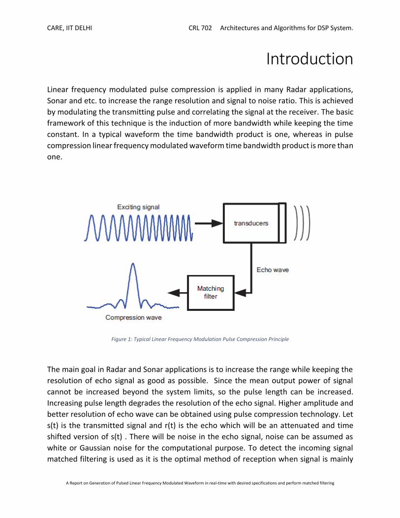
Linear frequency modulated pulse compression is applied in many Radar applications,

Sonar and etc. to increase the range resolution and signal to noise ratio. This is achieved

by modulating the transmitting pulse and correlating the signal at the receiver. The basic

framework of this technique is the induction of more bandwidth while keeping the time

constant. In a typical waveform the time bandwidth product is one, whereas in pulse

compression linear frequency modulated waveform time bandwidth product is more than

one.

Figure 1: Typical Linear Frequency Modulation Pulse Compression Principle

The main goal in Radar and Sonar applications is to increase the range while keeping the

resolution of echo signal as good as possible. Since the mean output power of signal

cannot be increased beyond the system limits, so the pulse length can be increased.

Increasing pulse length degrades the resolution of the echo signal. Higher amplitude and

better resolution of echo wave can be obtained using pulse compression technology. Let

s(t) is the transmitted signal and r(t) is the echo which will be an attenuated and time

shifted version of s(t) . There will be noise in the echo signal, noise can be assumed as

white or Gaussian noise for the computational purpose. To detect the incoming signal

matched filtering is used as it is the optimal method of reception when signal is mainly



corrupted by the additive Gaussian noise. In Matched filtering the incoming signal is

convolved with the time shifted version of the transmitted signal. This operation can be

done on the software.

To meet all the desire specification it is required to have a large enough pulse so that we

can have good SNR and at the same time it should not affect the resolution. Here Pulse

compression comes into Picture. The basic principle is that first the Signal is transmitted

with a long enough pulse which will not affect the energy budget. Then main concept is

in the designing of the pulse so that after matched filtering, the width of correlated signals

is smaller than the width obtained by standard sinusoidal pulse. That’s why this technique

is called pulse compression.

The working of a radar system can be summarized as, a short burst of radio frequency

energy is emitted from the directional antenna. Aircraft and other objects reflect some of

this energy back to a radio receiver located next to transmitter. Since radio waves travel

at a constant speed, the elapsed time between transmitted and received signal provides

the distance to the target. This brings up the first requirement for the pulse; it needs to

be as short as possible. For example a 1 microsecond pulse provides a radio burst about

300 meters long. This means that distance information we obtain with the system will

have a resolution of about the same length. If we want better resolution we need a

shorter pulse. The second requirement is obvious; if we want to detect objects farther

away, we need more energy in our pulse. But more energy and shorter pulse are

conflicting requirements. The electrical power needed to provide a pulse is equal to the

energy of the pulse divided by the pulse length. Requiring both more energy and a shorter

pulse makes electrical power handling a limiting factor in the system. And there is a limit

on the radio transmitter on power handling capabilities.

Chirp Signals provide a breaking of this limitation. For a rectangular pulse, the duration of

the transmitted pulse and the processed echo are effectively the same. Therefore, the

range resolution of the radar and the target detection capability are coupled in an inverse

relationship. Pulse compression techniques enable us to decouple the duration of the

pulse from its energy by effectively creating different durations for the transmitted pulse

and processed echo. Instead of bouncing an impulse off the target aircraft, a chirp signal

is used. After the chirp echo is received, it is matched filtered with the transmitted chirp

generating an impulse. Now a days this wave shaping of pulse has become a fundamental

part of radar system. In radar and sonar applications, linear chirps, which is a common

name for linear frequency modulated waveform, are typically used signals for the pulse

compression. The Chirp signals are the ingenious way of handling the echo resolution

problem in the radar and sonar applications.



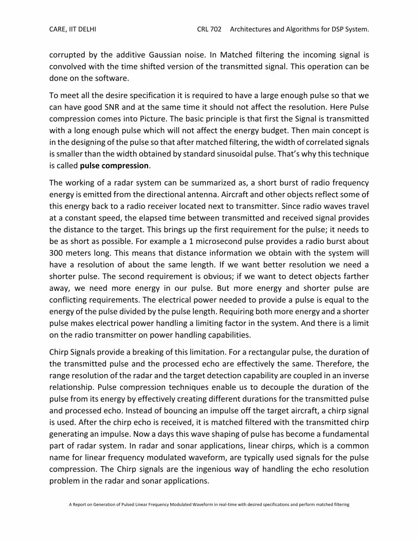
The Expression for the linear frequency modulated i.e. linear chirp is given by

𝑦[𝑛] = 𝐴 sin(2𝜋(𝑓𝑐 + 𝛼𝑛)𝑛)

Where A is the amplitude of the waveform,

fc is the start frequency,

α is the chirp rate,

n is the index value which ranges from 0 to N-1.

N is the no. of samples which is decided from the sampling rate.

The following figure shows a typical Linear Chirp signal with particular specifications.

Figure 2 Linear Chirp Signal

The waveform shown in figure 2 is observed to see that the frequency of the signal varies

from start frequency 20 Hz to end frequency 40 Hz. The waveform has a linear increase

in its frequency. The instantaneous frequency can be described as f = fc + kt.



Objective

The fundamental framework of this project was to generate the exciting signal that is

Pulsed linear frequency modulated waveform in real time with the desired specifications,

and perform the matched filtering. Sweep duration of the chirp is 1 second, which is also

the pulse duration. The sampling frequency is fixed at 500 Hz. For the test purpose chirp

rate and start frequency were chosen as 0.00008 and 0.04 respectively.

The following set of exercises were there:

1. Do a study for suitable method for waveform generation. How many clock cycles

are available on average to generate one sample of the waveform? Do an

estimation of the number of clock cycles that will be required by your algorithm to

generate one sample on average. Describe this exercise in your report.

2. Generate the waveform and display it on the oscilloscope. How many clock cycle

does it take to generate one pulse? You may generate a trigger pulse synchronized

with the start of the LFM waveform in another channel of the analog output to

stabilize the oscilloscope display.

3. Generate one LFM pulse of 1 second duration in Matlab using the expression for

PLFM for given specifications. The start frequency and chirp rate values are 0.04

and 0.0008 respectively. Generate and store the same pulse in the DSP memory

and copy it into Matlab. Obtain the mean square between the two waveforms in

Matlab. Explain the reasons for the m.s.e.

4. Extract one pulse length of waveform and perform matched filtering with a stored

replica of the waveform. Plot the output and mark the salient points of the

waveform. Compare it with the ideal output obtained in Matlab and explain the

differences.



Methods for function evaluation

Various methods for the evaluation of the function in the assembly language have been

studied. Some methods are listed below.

(i) Look up table Approach:

The most simple and crude approach to evaluate the function is to store all the

possible outcomes of the function in memory in the form of a table. It replaces all the

runtime computation by a simple indexing operation. The savings in terms of processing

time can be significant, since retrieving a value from memory is often faster than

undergoing an expensive computation. Whenever we want to compute any particular

value of function, we look up in the table for that respective value and fetch the data from

there in the program. Clearly resolution in this method is limited by the memory required

to store the look up table. Larger the lookup table, more is the computational complexity

as we need to search for that particular index in the look up table. We first computed the

function value using this method. In our case the possible outcome for the chirp signals

are 500 values. These values were generated using a Matlab code and stored in a memory

location. Particular sample value was located in the memory and chirp sample was

obtained and thus chirp waveform was observed in the DSK simulator. Obviously result

was having no error. But it is an impractical method as it is fixed for a particular set of

specifications and requires a lot of memory. Also, when searching for a particular sample,

it requires 500 searches that in turn increases the computational complexity. Although

the search complexity can be relaxed by using the methods such as binary search.



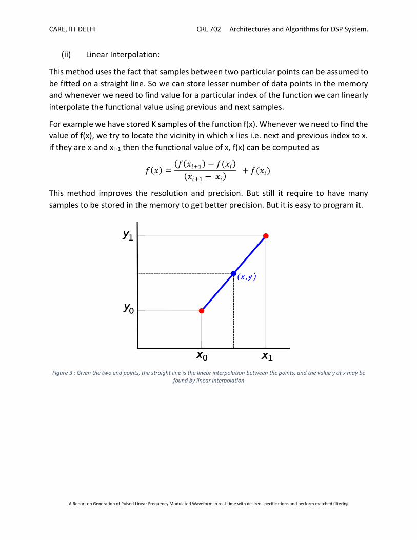
(ii) Linear Interpolation:

This method uses the fact that samples between two particular points can be assumed to

be fitted on a straight line. So we can store lesser number of data points in the memory

and whenever we need to find value for a particular index of the function we can linearly

interpolate the functional value using previous and next samples.

For example we have stored K samples of the function f(x). Whenever we need to find the

value of f(x), we try to locate the vicinity in which x lies i.e. next and previous index to x.

if they are xi and xi+1 then the functional value of x, f(x) can be computed as

𝑓(𝑥) =(𝑓(𝑥𝑖+1) − 𝑓(𝑥𝑖)

(𝑥𝑖+1 − 𝑥𝑖) + 𝑓(𝑥𝑖)

This method improves the resolution and precision. But still it require to have many

samples to be stored in the memory to get better precision. But it is easy to program it.

Figure 3 : Given the two end points, the straight line is the linear interpolation between the points, and the value y at x may be found by linear interpolation

http://upload.wikimedia.org/wikipedia/commons/d/dd/LinearInterpolation.svg



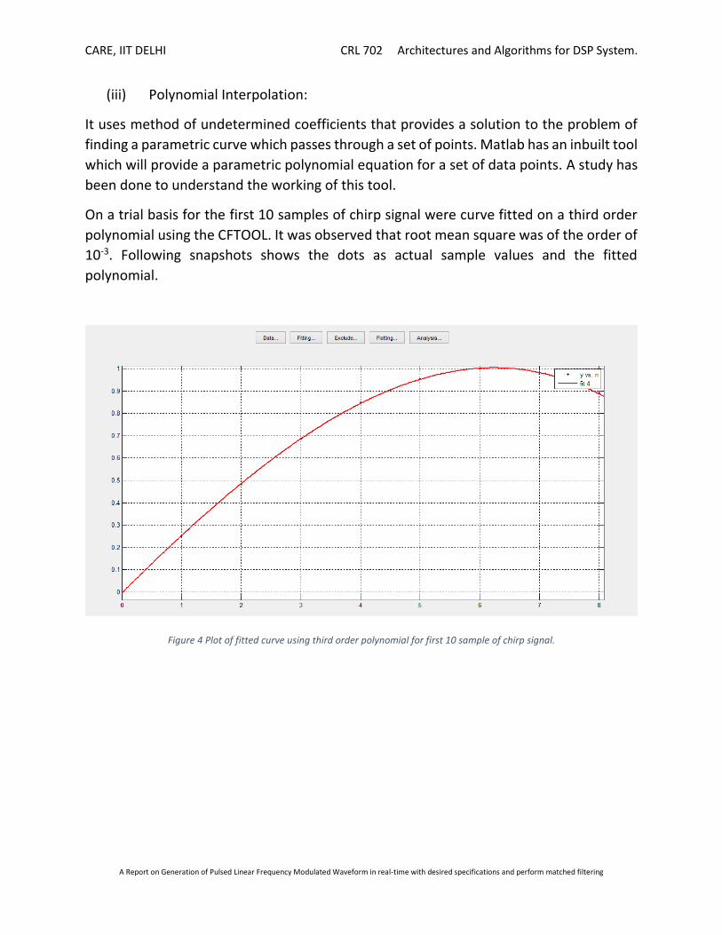
(iii) Polynomial Interpolation:

It uses method of undetermined coefficients that provides a solution to the problem of

finding a parametric curve which passes through a set of points. Matlab has an inbuilt tool

which will provide a parametric polynomial equation for a set of data points. A study has

been done to understand the working of this tool.

On a trial basis for the first 10 samples of chirp signal were curve fitted on a third order

polynomial using the CFTOOL. It was observed that root mean square was of the order of

10-3. Following snapshots shows the dots as actual sample values and the fitted

polynomial.

Figure 4 Plot of fitted curve using third order polynomial for first 10 sample of chirp signal.



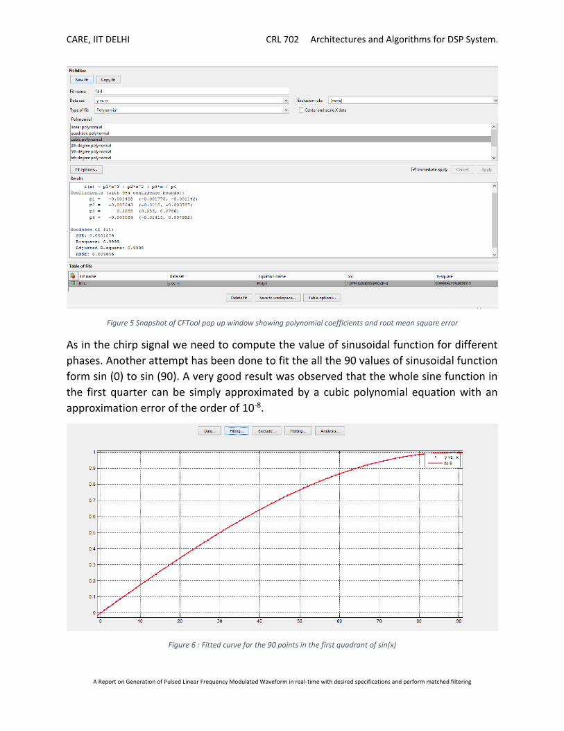
Figure 5 Snapshot of CFTool pop up window showing polynomial coefficients and root mean square error

As in the chirp signal we need to compute the value of sinusoidal function for different

phases. Another attempt has been done to fit the all the 90 values of sinusoidal function

form sin (0) to sin (90). A very good result was observed that the whole sine function in

the first quarter can be simply approximated by a cubic polynomial equation with an

approximation error of the order of 10-8.

Figure 6 : Fitted curve for the 90 points in the first quadrant of sin(x)



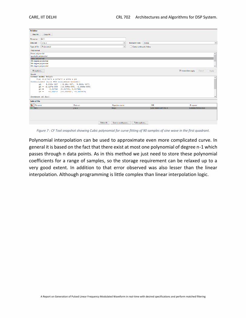
Figure 7 : CF Tool snapshot showing Cubic polynomial for curve fitting of 90 samples of sine wave in the first quadrant.

Polynomial interpolation can be used to approximate even more complicated curve. In

general it is based on the fact that there exist at most one polynomial of degree n-1 which

passes through n data points. As in this method we just need to store these polynomial

coefficients for a range of samples, so the storage requirement can be relaxed up to a

very good extent. In addition to that error observed was also lesser than the linear

interpolation. Although programming is little complex than linear interpolation logic.



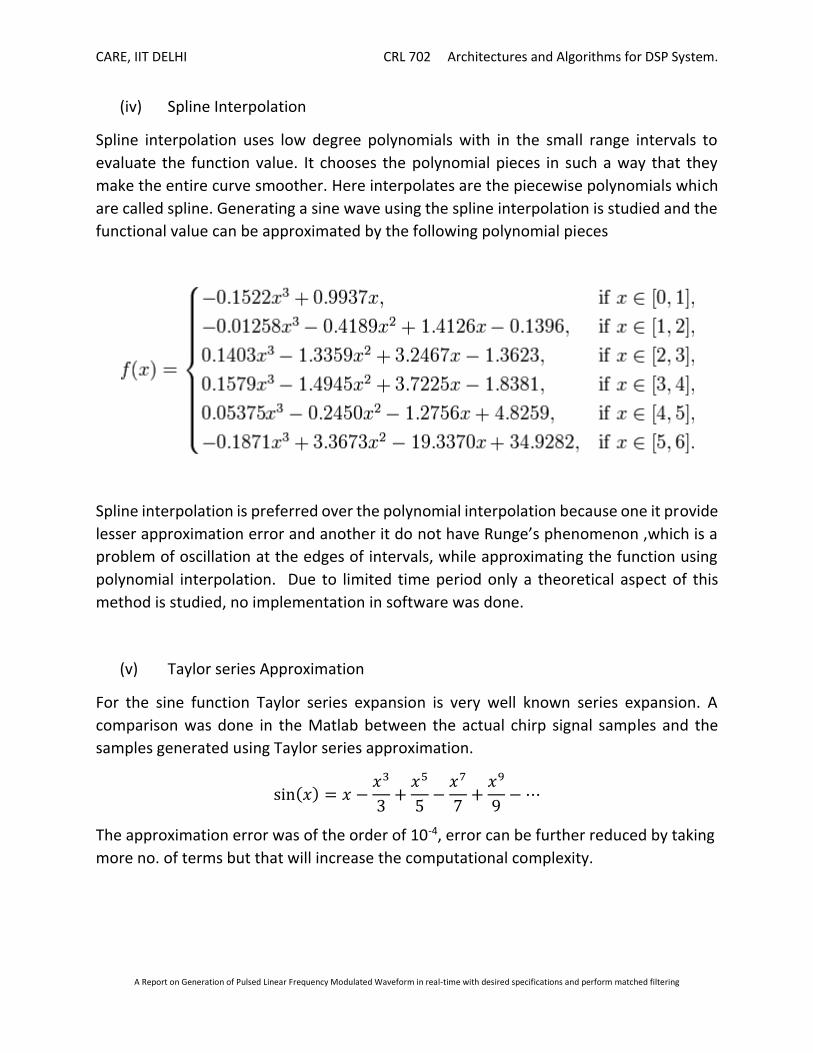
(iv) Spline Interpolation

Spline interpolation uses low degree polynomials with in the small range intervals to

evaluate the function value. It chooses the polynomial pieces in such a way that they

make the entire curve smoother. Here interpolates are the piecewise polynomials which

are called spline. Generating a sine wave using the spline interpolation is studied and the

functional value can be approximated by the following polynomial pieces

Spline interpolation is preferred over the polynomial interpolation because one it provide

lesser approximation error and another it do not have Runge’s phenomenon ,which is a

problem of oscillation at the edges of intervals, while approximating the function using

polynomial interpolation. Due to limited time period only a theoretical aspect of this

method is studied, no implementation in software was done.

(v) Taylor series Approximation

For the sine function Taylor series expansion is very well known series expansion. A

comparison was done in the Matlab between the actual chirp signal samples and the

samples generated using Taylor series approximation.

sin(𝑥) = 𝑥 −𝑥3

3+

𝑥5

5−

𝑥7

7+

𝑥9

9− ⋯

The approximation error was of the order of 10-4, error can be further reduced by taking

more no. of terms but that will increase the computational complexity.



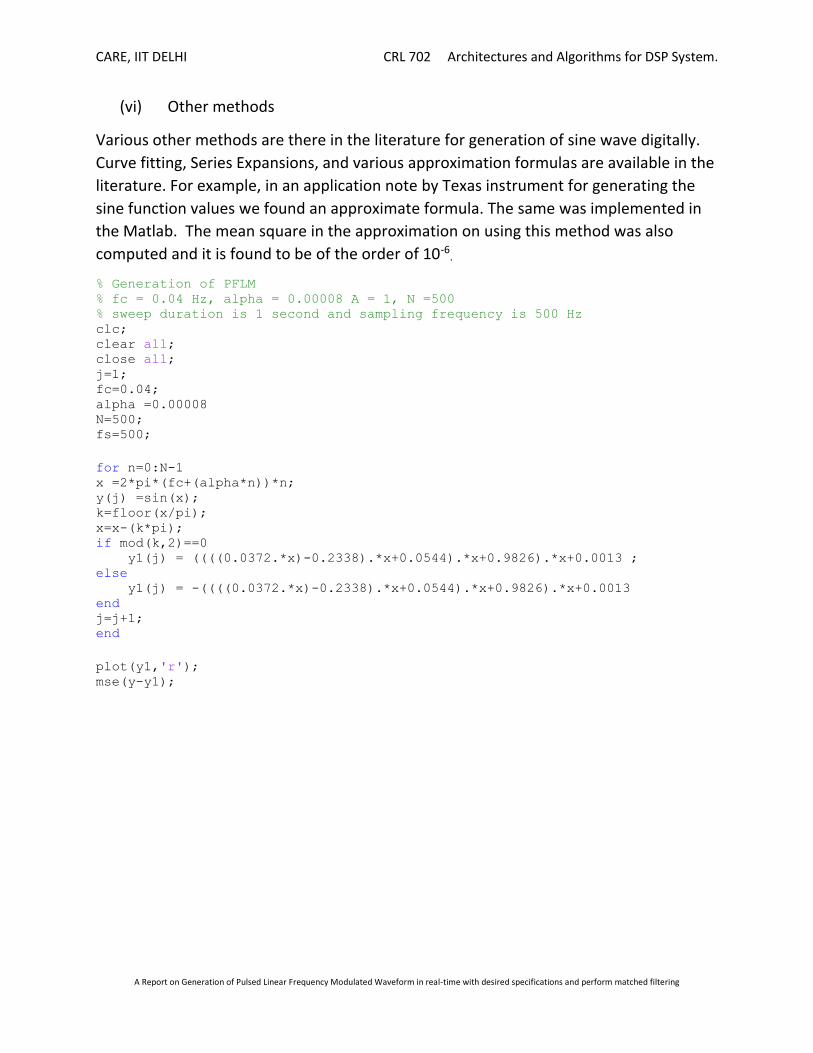
(vi) Other methods

Various other methods are there in the literature for generation of sine wave digitally.

Curve fitting, Series Expansions, and various approximation formulas are available in the

literature. For example, in an application note by Texas instrument for generating the

sine function values we found an approximate formula. The same was implemented in

the Matlab. The mean square in the approximation on using this method was also

computed and it is found to be of the order of 10-6.

% Generation of PFLM % fc = 0.04 Hz, alpha = 0.00008 A = 1, N =500 % sweep duration is 1 second and sampling frequency is 500 Hz clc;

clear all;

close all; j=1; fc=0.04; alpha =0.00008 N=500; fs=500;

for n=0:N-1 x =2*pi*(fc+(alpha*n))*n; y(j) =sin(x); k=floor(x/pi); x=x-(k*pi); if mod(k,2)==0 y1(j) = ((((0.0372.*x)-0.2338).*x+0.0544).*x+0.9826).*x+0.0013 ; else y1(j) = -((((0.0372.*x)-0.2338).*x+0.0544).*x+0.9826).*x+0.0013 end j=j+1; end

plot(y1,'r'); mse(y-y1);



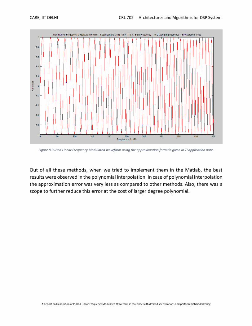
Figure 8 Pulsed Linear Frequency Modulated waveform using the approximation formula given in TI application note.

Out of all these methods, when we tried to implement them in the Matlab, the best

results were observed in the polynomial interpolation. In case of polynomial interpolation

the approximation error was very less as compared to other methods. Also, there was a

scope to further reduce this error at the cost of larger degree polynomial.



Generation of chirp signal samples in the TMS320C5510 kit.

The first objective of the project was to write an efficient assembly language program to

generate the 500 samples of the chirp signal. This first thing is to choose the optimum Q

format for various variables in the program.

Choice of Q- Format:

For the chirp rate, the magnitude of the variables was of the order of 10-5. To store such

small magnitude value the first choice will be Q15, but that too results in a very bad

approximation. As, the given chirp rate magnitude for test purpose was 8 X 10-5. If we

store it in Q15 format it will be 2.62144 which on rounding will become 3. On converting

back 3 to fractional value it results in 9.15 X 10-5, that is an error of more than 10%. This

is not a tolerable error. So instead of typical Q15 format, Q28 format was chosen.

For start frequency Q15 format was chosen. The index numbers are stored in Q0 format.

Since the final frequency value is getting multiplied with the 2π, so there is no need to

store the integer part of the frequency and only fractional value can do the job.

Choice of method:

This was a very crucial step as it decides the approximation error as well as complexity of

the program. First polynomial interpolation method was tried, But the main problem was

the limited size of registers in the DSK kit, as in polynomial interpolation we need to

compute up to 3rd or 4th power of the phase of sine function. Since we don’t have that

much long registers which can store the results of these computation’s outcome, so

ultimately we are losing the precision. Linear interpolation method was providing larger

error as compared to polynomial interpolation method (as compared in Matlab), however

while performing the both in the DSK kit there was no significant improvement in terms

of lesser error whereas he computation complexity was increasing significantly. Also,

Runge phenomenon was a bigger problem in the polynomial interpolation. So finally we

decided to go with an optimum linear interpolation method.



Finally two main methods were chosen

a. Direct look up using optimum Linear interpolation approach which is providing

minimum harmonic distortion

b. Approximation of sine function using a mathematical series function.

Both the methods were implemented in the DSK kit and in case of optimum linear

interpolation method error was found lesser. Both the methods have different

constraints. Direct look up method is fast with minimal errors but requires significant Rom

storage. The mathematical series method is fast and requires minimal ROM storage but

results in less precision. The same results were obtained in Matlab. The reason behind

using the optimum word with linear interpolation repeatedly is that, we have also

exploited the properties of the sinusoidal function to make the computation easier as well

as to save the storage requirement for linear interpolation.

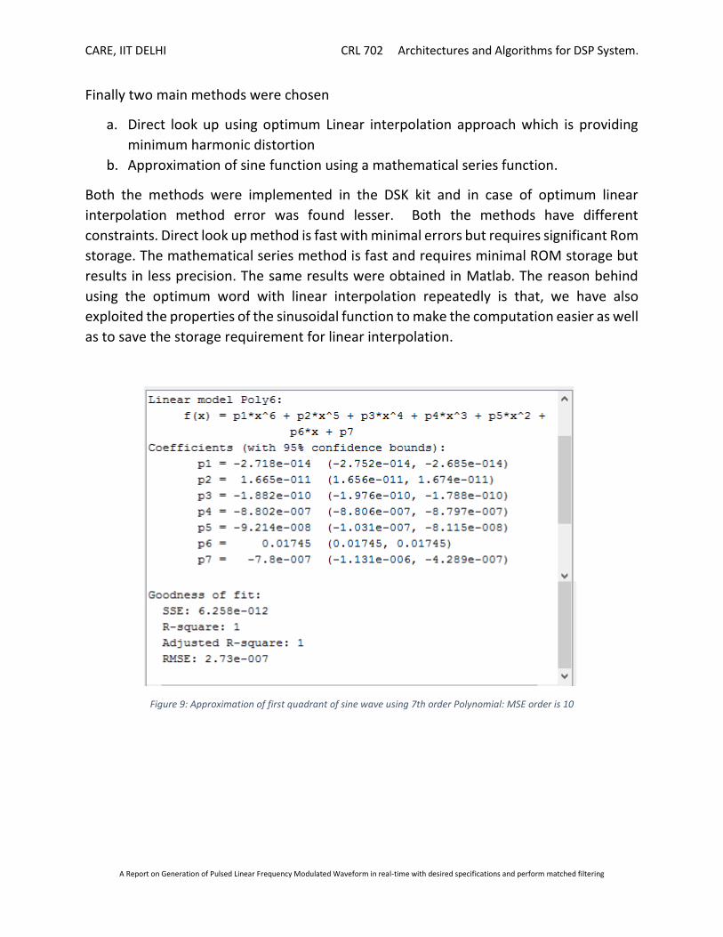
Figure 9: Approximation of first quadrant of sine wave using 7th order Polynomial: MSE order is 10



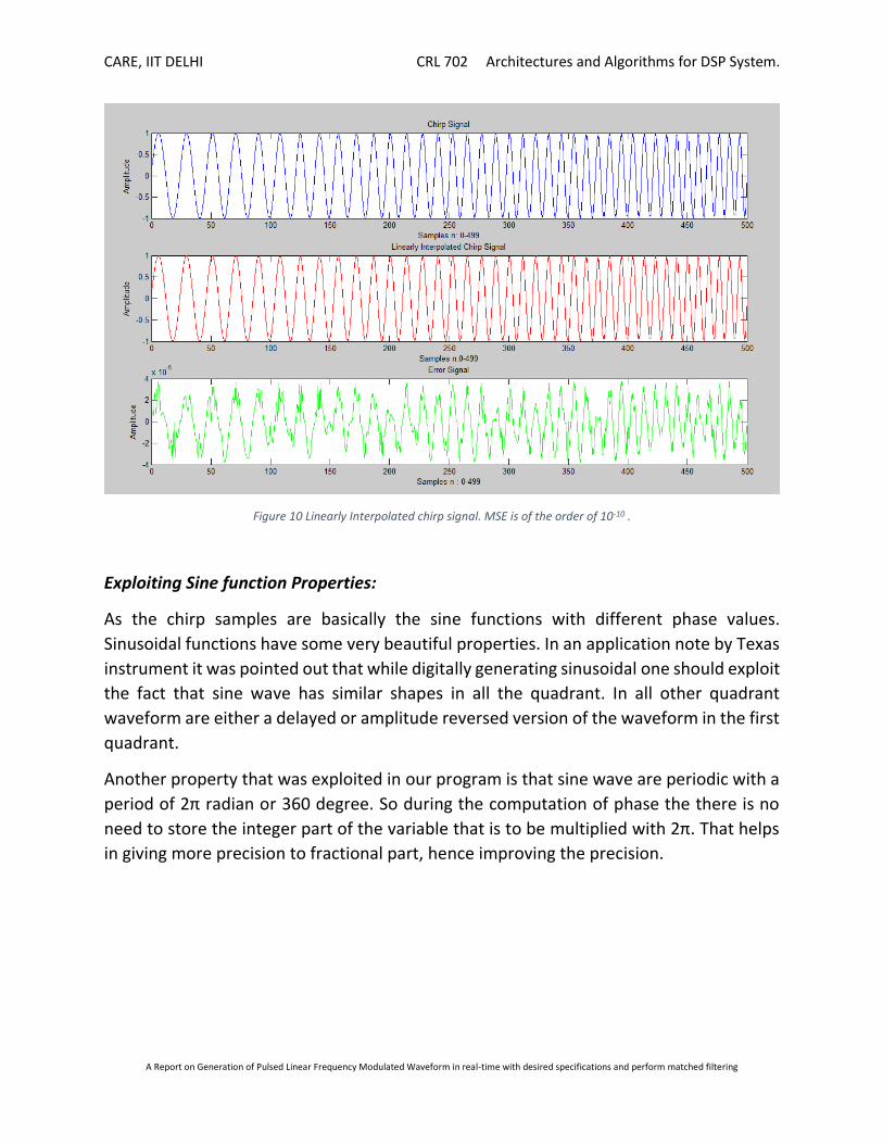
Figure 10 Linearly Interpolated chirp signal. MSE is of the order of 10-10 .

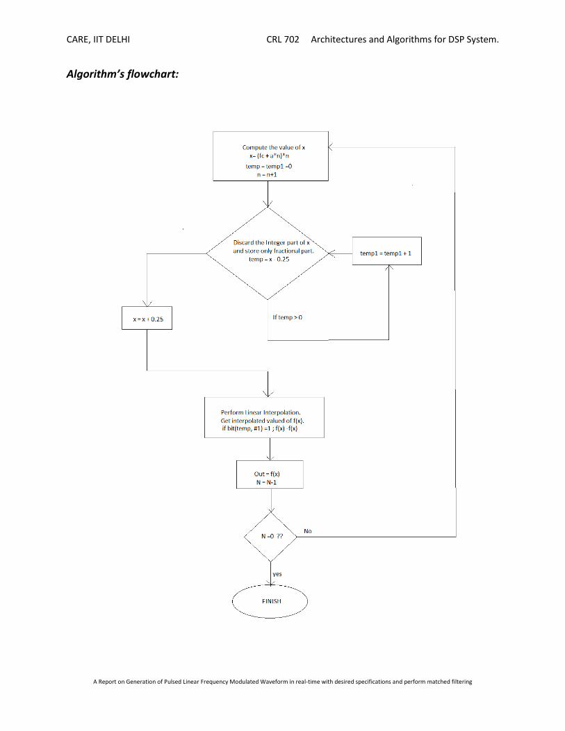
Exploiting Sine function Properties:

As the chirp samples are basically the sine functions with different phase values.

Sinusoidal functions have some very beautiful properties. In an application note by Texas

instrument it was pointed out that while digitally generating sinusoidal one should exploit

the fact that sine wave has similar shapes in all the quadrant. In all other quadrant

waveform are either a delayed or amplitude reversed version of the waveform in the first

quadrant.

Another property that was exploited in our program is that sine wave are periodic with a

period of 2π radian or 360 degree. So during the computation of phase the there is no

need to store the integer part of the variable that is to be multiplied with 2π. That helps

in giving more precision to fractional part, hence improving the precision.



Algorithm’s flowchart:



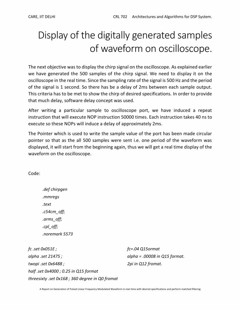
Display of the digitally generated samples of waveform on oscilloscope.

The next objective was to display the chirp signal on the oscilloscope. As explained earlier

we have generated the 500 samples of the chirp signal. We need to display it on the

oscilloscope in the real time. Since the sampling rate of the signal is 500 Hz and the period

of the signal is 1 second. So there has be a delay of 2ms between each sample output.

This criteria has to be met to show the chirp of desired specifications. In order to provide

that much delay, software delay concept was used.

After writing a particular sample to oscilloscope port, we have induced a repeat

instruction that will execute NOP instruction 50000 times. Each instruction takes 40 ns to

execute so these NOPs will induce a delay of approximately 2ms.

The Pointer which is used to write the sample value of the port has been made circular

pointer so that as the all 500 samples were sent i.e. one period of the waveform was

displayed, it will start from the beginning again, thus we will get a real time display of the

waveform on the oscilloscope.

Code:

.def chirpgen

.mmregs

.text

.c54cm_off;

.arms_off;

.cpl_off;

.noremark 5573

fc .set 0x051E ; fc=.04 Q15ormat

alpha .set 21475 ; alpha = .00008 in Q15 format.

twopi .set 0x6488 ; 2pi in Q12 fromat.

half .set 0x4000 ; 0.25 in Q15 format

threesixty .set 0x168 ; 360 degree in Q0 fromat



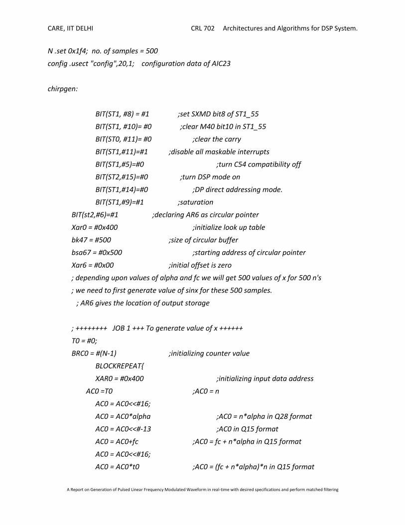
N .set 0x1f4; no. of samples = 500

config .usect "config",20,1; configuration data of AIC23

chirpgen:

BIT(ST1, #8) = #1 ;set SXMD bit8 of ST1_55

BIT(ST1, #10)= #0 ;clear M40 bit10 in ST1_55

BIT(ST0, #11)= #0 ;clear the carry

BIT(ST1,#11)=#1 ;disable all maskable interrupts

BIT(ST1,#5)=#0 ;turn C54 compatibility off

BIT(ST2,#15)=#0 ;turn DSP mode on

BIT(ST1,#14)=#0 ;DP direct addressing mode.

BIT(ST1,#9)=#1 ;saturation

BIT(st2,#6)=#1 ;declaring AR6 as circular pointer

Xar0 = #0x400 ;initialize look up table

bk47 = #500 ;size of circular buffer

bsa67 = #0x500 ;starting address of circular pointer

Xar6 = #0x00 ;initial offset is zero

; depending upon values of alpha and fc we will get 500 values of x for 500 n's

; we need to first generate value of sinx for these 500 samples.

; AR6 gives the location of output storage

; ++++++++ JOB 1 +++ To generate value of x ++++++

T0 = #0;

BRC0 = #(N-1) ;initializing counter value

BLOCKREPEAT{

XAR0 = #0x400 ;initializing input data address

AC0 =T0 ;AC0 = n

AC0 = AC0<<#16;

AC0 = AC0*alpha ;AC0 = n*alpha in Q28 format

AC0 = AC0<<#-13 ;AC0 in Q15 format

AC0 = AC0+fc ;AC0 = fc + n*alpha in Q15 format

AC0 = AC0<<#16;

AC0 = AC0*t0 ;AC0 = (fc + n*alpha)*n in Q15 format



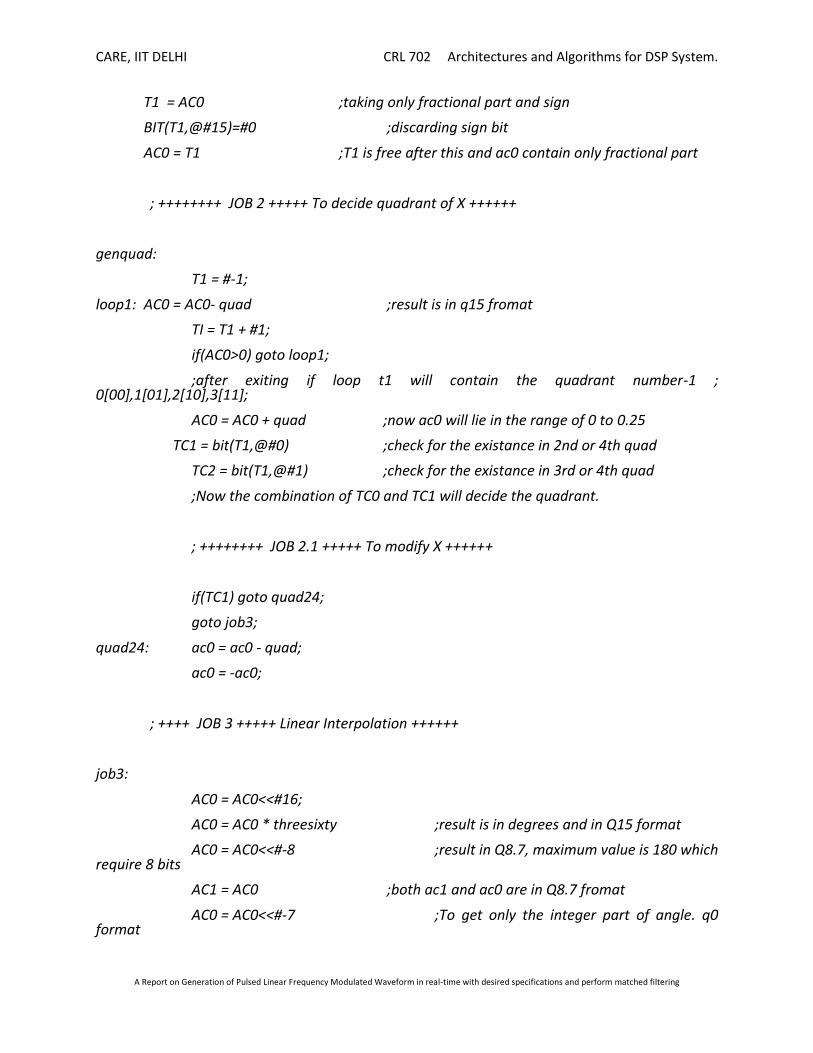
T1 = AC0 ;taking only fractional part and sign

BIT(T1,@#15)=#0 ;discarding sign bit

AC0 = T1 ;T1 is free after this and ac0 contain only fractional part

; ++++++++ JOB 2 +++++ To decide quadrant of X ++++++

genquad:

T1 = #-1;

loop1: AC0 = AC0- quad ;result is in q15 fromat

TI = T1 + #1;

if(AC0>0) goto loop1;

;after exiting if loop t1 will contain the quadrant number-1 ; 0[00],1[01],2[10],3[11];

AC0 = AC0 + quad ;now ac0 will lie in the range of 0 to 0.25

TC1 = bit(T1,@#0) ;check for the existance in 2nd or 4th quad

TC2 = bit(T1,@#1) ;check for the existance in 3rd or 4th quad

;Now the combination of TC0 and TC1 will decide the quadrant.

; ++++++++ JOB 2.1 +++++ To modify X ++++++

if(TC1) goto quad24;

goto job3;

quad24: ac0 = ac0 - quad;

ac0 = -ac0;

; ++++ JOB 3 +++++ Linear Interpolation ++++++

job3:

AC0 = AC0<<#16;

AC0 = AC0 * threesixty ;result is in degrees and in Q15 format

AC0 = AC0<<#-8 ;result in Q8.7, maximum value is 180 which require 8 bits

AC1 = AC0 ;both ac1 and ac0 are in Q8.7 fromat

AC0 = AC0<<#-7 ;To get only the integer part of angle. q0 format



AR2 = AR0;

T3 = #0;

AR2 = AR2 + AC0 ;To get Xk ar0 is having Q0 fromat

T3 = T3+1;

AR0 = AR2;

AC0 = AC0<<#7 ;ac0 is gain in Q8.7 format

AC2 = AC1;

AC1 = AC1 - AC0 ;To get x-Xk result is in q7.8 format . ac2 is free

AC0 = AC1;

AC2 = *+AR0 ;AC2 will have f(Xk+1) result is in q0.15 format

AC2 = AC2 - *-AR0 ;AC2 will have f(XK+1)-f(Xk) Q0.15 fromat

AC0 = AC0<<#16;

AC2 = AC2<<#16;

AC0 = AC0 * ac2 ;the result is in Q8*Q15 = Q23 fromat

AC0 = AC0<<#-8 ;the result is again in Q0.15 format

AC0 = AC0 + *AR0 ;f(x) the result is in Q0.15 fromat

if(TC1) goto quadne;

goto quadpo;

quadne: ac0 = -ac0;

quadpo: ac0 = ac0;

*ar6+ = ac0;

t0 = t0 +1;

}

;*******************************

; Open the codec

;*******************************

;This configures the McBSPs to communicate with an AIC23 codec.

;McBSP1 is used in Master SPI format as the control channel with clocks being

;coming from the internal sample rate generator. McBSP2 is the data

;channel. It is used in slave mode using the codec's bi-directional



;DSP data format. Each sample consists of one frame with two 16-bit

;elements corresponding to left and right. Clocks and frame syncs on

;the data channel are generated by the AIC23 external to the DSP.

;======== mcbspCfg1 ========

;Create a mcbsp configuration object use for the mcbsp1 talking

;to the aic23 codec. The format is SPI with 16-bit frames. All clocks

;and frame syncs are generated internally.

;AR0 -> McBSP1 registers.

XAR0 = #2C04h

*AR0+ = #0100h || writeport();SPCR2_1


*AR0+ = #0000h || writeport();RCR2_1


*AR0+ = #0000h || writeport();XCR2_1


*AR0+ = #2013h || writeport();SRGR2_1


AR0 += #6;

*AR0 = #1A0Ah || writeport();PCR_1

AR0 -= #6;

;Start McBSP by setting Trasmitter bit to 1

AR0 = #2C04h;SPCR2_1

*AR0 = #0101h || writeport();

;*******************************

;configuration of the AIC23 registers

;*************************************************************************

; Configure the DMA Channel 0 to send the register values to AIC via McBSP1



; Channel 0 is used for data transfer from SARAM port to McBSP #1 port

;************************************************************************

;DMA Global Control Register

XAR1 = #0E00h;

*AR1 = #4h || writeport(); Global Control Register FREE=1

; AR1 -> DMA channel_0

XAR4 = #config ;AR4 -> Source

XAR5 = #2C03h ; AR5 -> Destination

XAR1 = #0C00h ; AR2 -> DMA channel_0 register

*AR1+ = #0601h || writeport();CSDP_0

*AR1+ = #1046h || writeport();CCR disable channel-0 and cofigure

;the reg with auto-increment of address

*AR1+ = #8h || writeport(); CICR_0;

*AR1+ = #0 || writeport(); clear the CSR register

AC0 = XAR4 ;

AC1 = AC0 << #1;

*AR1+ = LO(AC1 << #0) || writeport();Source byte address

*AR1+ = HI(AC1 << #0) || writeport();Source 'config'

AC0 = XAR5 ;

AC1 = AC0 << #1;

*AR1+ = LO(AC1 << #0) || writeport();Peripheral byte address

*AR1+ = HI(AC1 << #0) || writeport();Destination DXR1_0

*AR1+ = #0Bh || writeport();DMA_CEN Number of 16bit word to be transferred

;/transmitted

*AR1+ = #01h || writeport();DMA_CFN Number of frames per block

*AR1+ = #0h || writeport();DMA_CEI

*AR1 = #0h || writeport(); DMA_CFI



;Prime DXR by writing first element

AR0 = #2C03h;

*AR0+ = #8000h || writeport();

;Enable channel_0

AR1 = #0C01h;

*AR1 = #10C6h || writeport();

;Start Sample Rate Generator and Enable Frame Sync Logic

*AR0 = #03C1h || writeport(); SPCR2_0

;Allow Sample Rate Generator to Stablize

BRC0 = #35h

BLOCKREPEAT{

NOP;

NOP;

NOP;

NOP;

NOP;

NOP;

NOP;

NOP;

NOP;

NOP;

NOP;

NOP;

}

;***************************************************************

;This section configures MCBSP2 for 32-bit frames consisting of a

;16-bit word for each of the left and right channels.

;The AIC23 is in master mode, DSP format and generates clocks



;and frame syncs externally.

; ======== mcbspCfg2 ========

; Create a mcbsp configuration object use for the mcbsp2 talking

; to the aic23 codec.

; AR0 -> McBSP2 registers.

;************************************************************

XAR0 = #3004h









AR0 += #6;

*AR0 = #0003h || writeport();PCR_2

AR0 -= #6;

;Start McBSP by setting Trasmitter and Receiver bit to 1

AR0 = #3004h; SPCR2_2

*AR0+ = #0101h || writeport();XRST_ = 1

*AR0 = #0001h || writeport();RRST_ = 1

;Prime DRR by reading first element

AR0 = #3001h;

AC0 = *AR0 || readport();

;Prime DXR by writing first element

AR0 = #3003h;

*AR0 = AC0 || writeport();

;Start Sample Rate Generator and Enable Frame Sync Logic



AR0 = #3004h;

*AR0 = #03C1h || writeport();

;Allow Sample Rate Generator to Stablize

BRC0 = #35h

BLOCKREPEAT{

NOP;

NOP;

NOP;

NOP;

NOP;

NOP;

NOP;

NOP;

NOP;

NOP;

NOP;

NOP;

}

;*****************************

; Read a data sample and wirte it to codec

;******************************

AR0 = #3003h

AR2 = #3001h;

loop_13:T1 = *port(#3005h);

T2=*AR6+;

loop_131:T0 = *port(#3004h);

; poll whether the word is ready ot transmit

TC1 = BIT( T0, @#1);xrdy

TC2 = BIT( T0, @#2);xempty

IF( !TC1 | TC2 ) GOTO loop_131;

; set the register with value in AC1

*AR0 = T2 || writeport();



repeat(65535)

nop;

repeat(65535)

nop;

repeat(65535)

nop;

repeat(65535)

nop;

repeat(65535)

nop;

goto loop_13;

;*****************************

; close the codec

;******************************

AR0 = #2C03h

AC0 = #6;

AC1 = #00ffh;

AC1 = AC1 | (AC0 <<< 9);

; poll whether the word have been transmitted before u transmit next

loop_3:T0 = *port(#2C04h);

TC1 = BIT( T0, @#1);xrdy

TC2 = BIT( T0, @#2);xempty

IF( !TC1 | TC2 ) GOTO loop_3;

; set the register with value in AC1

*AR0 = AC1 || writeport();

idle;

nop;

nop;

.end;



As per asked in the exercise 1 and 2, an intensive study was done for the different

methods of generation of waveform. Finally an optimum linear interpolation method

which smartly exploits the properties of sinusoidal function, was chosen. 500 samples of

the chirp signal that is samples for the one period of the chirp were successfully generated

using the code composer studio. Code for this is already attached. The code was explained

as when required with the use of ample of comments. An algorithm flow chart was also

attached to get a basic overview of the logic implemented in the program.

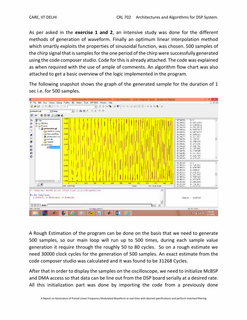
The following snapshot shows the graph of the generated sample for the duration of 1

sec i.e. for 500 samples.

A Rough Estimation of the program can be done on the basis that we need to generate

500 samples, so our main loop will run up to 500 times, during each sample value

generation it require through the roughly 50 to 80 cycles. So on a rough estimate we

need 30000 clock cycles for the generation of 500 samples. An exact estimate from the

code composer studio was calculated and it was found to be 31268 Cycles.

After that in order to display the samples on the oscilloscope, we need to initialize McBSP

and DMA access so that data can be line out from the DSP board serially at a desired rate.

All this initialization part was done by importing the code from a previously done



experiment. This Initialization can be treated as overhead and it was found that it require

1012 additional clock cycles. After that we need to write the data to port. While writing

the data to port, we need to ensure that there should be appropriate delay between the

two successive samples write up operation, so that the sampling rate criteria is not

violated. As in total we had 500 samples and we need to display these samples in 1

second. So between two samples there has to be a delay of 2ms. This 2ms delay is

provided just after the writing operation to port. In order to have a delay of 2ms, we need

to induce around 400,000 clock cycles. (C55 operates at the rate of 200 MHz, so it require

5 ns for a clock cycle.) The waveform observed on the output of oscilloscope appear as a

running waveform. In order to stabilize it a trigger may be generated.



Computation of Mean square error

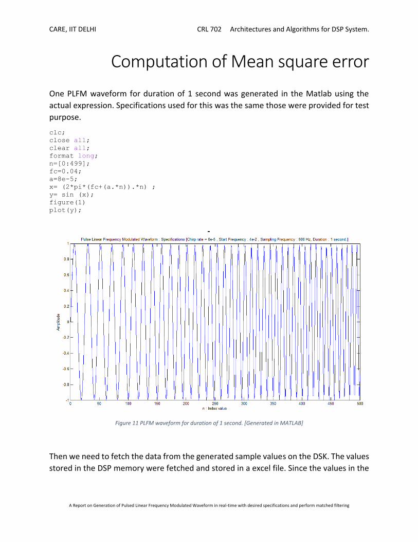
One PLFM waveform for duration of 1 second was generated in the Matlab using the

actual expression. Specifications used for this was the same those were provided for test

purpose.

clc; close all; clear all; format long; n=[0:499]; fc=0.04; a=8e-5; x= (2*pi*(fc+(a.*n)).*n) ; y= sin (x); figure(1) plot(y);

Figure 11 PLFM waveform for duration of 1 second. [Generated in MATLAB]

Then we need to fetch the data from the generated sample values on the DSK. The values

stored in the DSP memory were fetched and stored in a excel file. Since the values in the



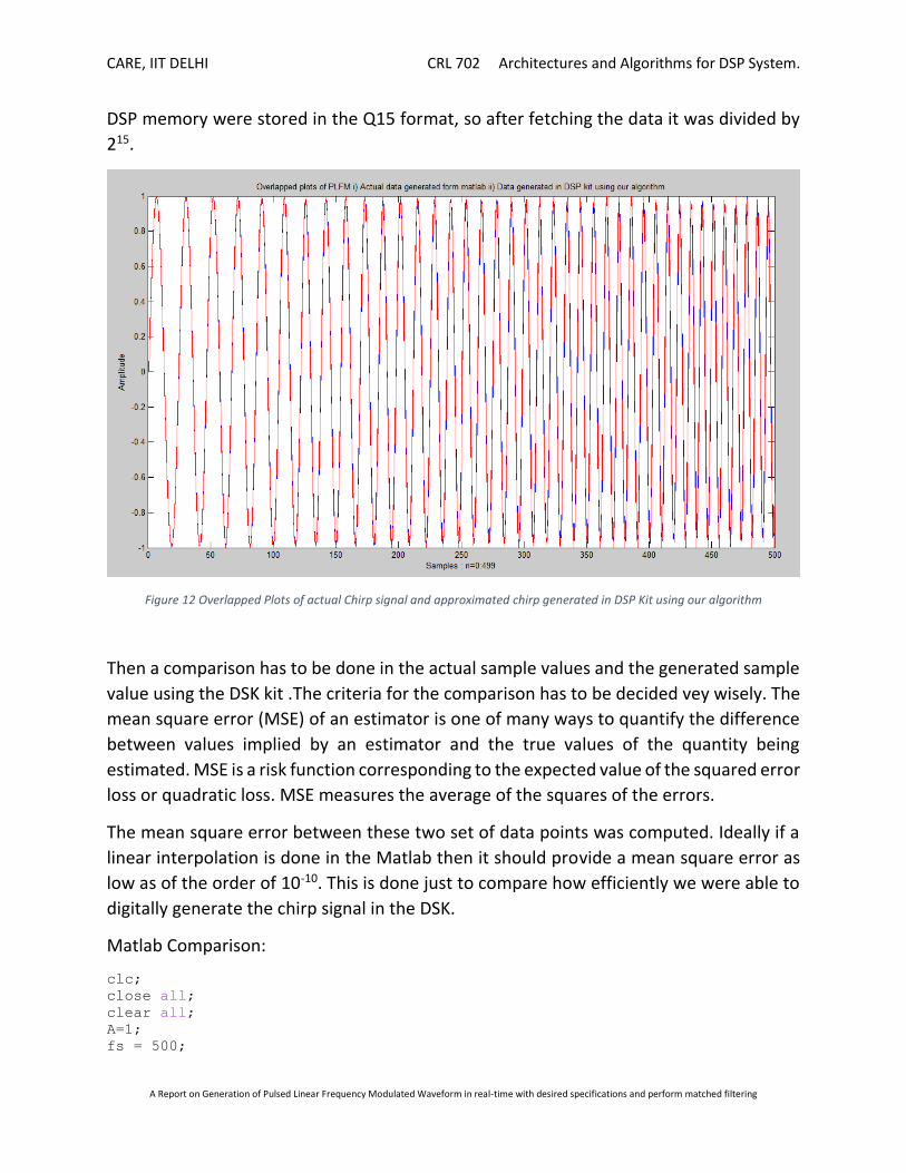
DSP memory were stored in the Q15 format, so after fetching the data it was divided by

215.

Figure 12 Overlapped Plots of actual Chirp signal and approximated chirp generated in DSP Kit using our algorithm

Then a comparison has to be done in the actual sample values and the generated sample

value using the DSK kit .The criteria for the comparison has to be decided vey wisely. The

mean square error (MSE) of an estimator is one of many ways to quantify the difference

between values implied by an estimator and the true values of the quantity being

estimated. MSE is a risk function corresponding to the expected value of the squared error

loss or quadratic loss. MSE measures the average of the squares of the errors.

The mean square error between these two set of data points was computed. Ideally if a

linear interpolation is done in the Matlab then it should provide a mean square error as

low as of the order of 10-10. This is done just to compare how efficiently we were able to

digitally generate the chirp signal in the DSK.

Matlab Comparison:

clc; close all; clear all; A=1; fs = 500;



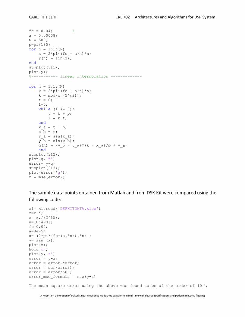
fc = 0.04; % a = 0.00008; N = 500; p=pi/180; for n = 1:1:(N) x = 2*pi*(fc + a*n)*n; y(n) = sin(x); end subplot(311); plot(y); %----------- linear interpolation -------------

for n = 1:1:(N) x = 2*pi*(fc + a*n)*n; k = mod(x,(2*pi)); t = 0; l=0; while (l >= 0); t = t + p; l = k-t; end x_a = t - p; x_b = t; y_a = sin(x_a); y_b = sin(x_b); q(n) = (y_b - y_a)*(k - x_a)/p + y_a; end subplot(312); plot(q,'r') error= y-q; subplot(313); plot(error,'g'); m = mse(error);

The sample data points obtained from Matlab and from DSK Kit were compared using the

following code:

z1= xlsread('DSPKITDATA.xlsx') z=z1'; z= z./(2^15); n=[0:499]; fc=0.04; a=8e-5; x= (2*pi*(fc+(a.*n)).*n) ; y= sin (x); plot(z); hold on; plot(y,'r') error = y-z; error = error.*error; error = sum(error); error = error/500; error_mse_formula = mse(y-z)

The mean square error using the above was found to be of the order of 10-3.



Matched filtering

The final objective was to extract one pulse length of the waveform and perform matched

filtering with a stored replica of the waveform. The matched filter design was

implemented in the DSK by performing the correlation of the digitally generated signal

with the reference signal generated in the Matlab. Here this can be assumed to be

analogous to the fact that reference signal generated in Matlab is transmitted signal and

signal generated in the DSK kit is the received echo of the signal which actually is

transmitted signal plus some additive noise. The additive noise here is in the form of the

precision lost during generation of the waveform in DSK. On performing the matched

filtering of two same signal ideally there should be

A correlation is basically a form of convolution where the second signal is only the delayed

version of the primary signal, in case of matched filtering this delay is kept equal to the

time period of the signal. So to perform matched filtering in software instead of doing

convolution in a typical fashion where we multiply the first sample with the last sample

of the second signal and perform the cross multiplication of the successive samples in a

zigzag fashion, here we need to perform simply the parallel multiplication between the

data points and accumulate them after multiplication of all the corresponding samples

with their counterpart samples in the reference or transmitted pulse.

The matched filtering was performed using the software as follows:

.def matched_filter

.mmregs

.text

.c54cm_off;

.arms_off;

.cpl_off;

matched_filter:

bit(ST1, #8) = #1; set SXMD bit8 of ST1_55

bit(ST1, #9) = #1 ; set SATD bit9 of ST1_55

bit(ST1, #10) = #0; clear M40 bit10 in ST1_55

xar0= #0xc000; initial address of data



ar1= ar0 + #499; last address of data

ar4 = ar1;

xar2 = #ydat;

t0 = #0;

t1 = #998;

again:

brc0 = t0;

ac0 = #0;

;ar0 = ar0 - t0;

;ar1 = ar1 + t0;

blockrepeat{

ac1 = *ar0-;

ac1 = ac1<<#16;

ac1 = ac1 * *ar1-;

ac1 = ac1<<#-15;

ac0 = ac0 + ac1;

}

xar0 = #0xc000;

ar0 = ar0+t0;

ar1 = ar4;

ac0 = ac0<<#-8;

*ar2+ = ac0;

t0 = t0 +#1;

t1 = t1 -#1;

;tc1= (t1>#0);

if(t1>#0) goto again

idle;

.end

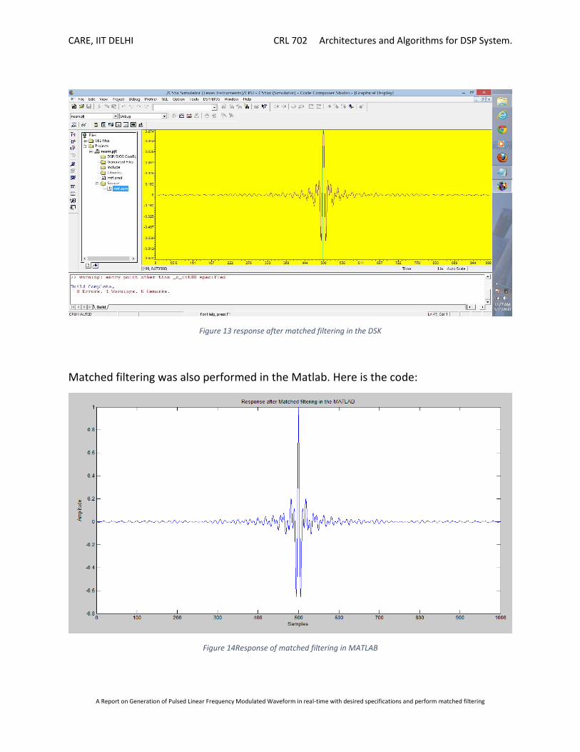
The results obtained on performing the matched filtering between extracted one pulse length of waveform and stored replica of the waveform were as follows:



Figure 13 response after matched filtering in the DSK

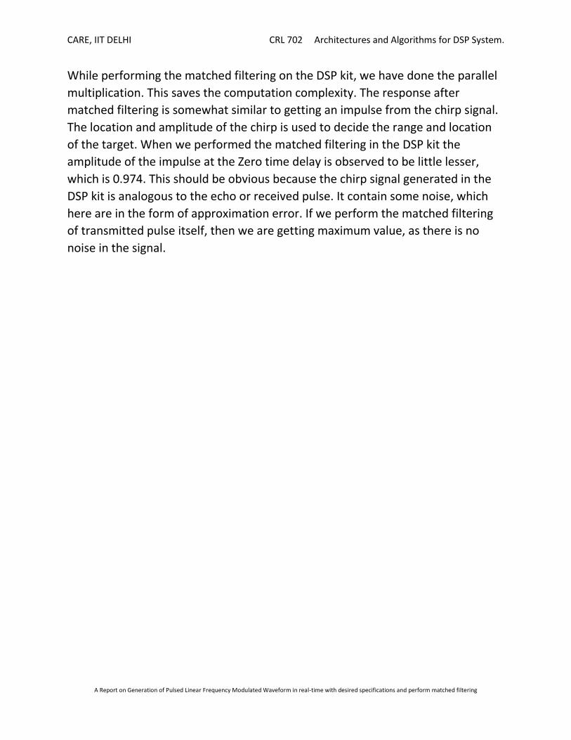
Matched filtering was also performed in the Matlab. Here is the code:

Figure 14Response of matched filtering in MATLAB



While performing the matched filtering on the DSP kit, we have done the parallel

multiplication. This saves the computation complexity. The response after

matched filtering is somewhat similar to getting an impulse from the chirp signal.

The location and amplitude of the chirp is used to decide the range and location

of the target. When we performed the matched filtering in the DSP kit the

amplitude of the impulse at the Zero time delay is observed to be little lesser,

which is 0.974. This should be obvious because the chirp signal generated in the

DSP kit is analogous to the echo or received pulse. It contain some noise, which

here are in the form of approximation error. If we perform the matched filtering

of transmitted pulse itself, then we are getting maximum value, as there is no

noise in the signal.

Generation of real time plfm waveform in tms320c5510 processo girish iit delhi

Documents

Transcript of Generation of real time plfm waveform in tms320c5510 processo girish iit delhi