GENERATION OF AN EARLY WARNING SYSTEM FOR …etd.lib.metu.edu.tr/upload/12619095/index.pdf · Fiber...

GENERATION OF AN EARLY WARNING SYSTEM FOR LANDSLIDE AND

SLOPE INSTABILITY BY OPTICAL FIBER TECHNOLOGY

A THESIS SUBMITTED TO

THE GRADUATE SCHOOL OF NATURAL AND APPLIED SCIENCES

OF

MIDDLE EAST TECHNICAL UNIVERSITY

BY

ARZU ARSLAN

IN PARTIAL FULFILLMENT OF THE REQUIREMENTS

FOR

THE DEGREE OF MASTER OF SCIENCE

IN

GEOLOGICAL ENGINEERING

AUGUST 2015

iii

Approval of the thesis:

GENERATION OF AN EARLY WARNING SYSTEM FOR LANDSLIDE

AND SLOPE INSTABILITY BY OPTICAL FIBER TECHNOLOGY

Submitted by ARZU ARSLAN in partial fulfillment of the requirements for the

degree of Master of Science in Geological Engineering Department, Middle East

Technical University by,

Prof. Dr. Gülbin Dural Ünver ____________________

Dean, Graduate School of Natural and Applied Sciences

Prof. Dr. Erdin Bozkurt ____________________

Head of Department, Geological Engineering

Prof. Dr. Haluk Akgün ____________________

Supervisor, Geological Engineering Dept., METU

Examining Committee Members:

Prof. Dr. Erdal Çokça ____________________

Civil Engineering Dept., METU

Prof. Dr. Haluk Akgün ____________________

Geological Engineering Dept., METU

Assoc. Prof. Dr. M. Tolga Yılmaz ____________________

Engineering Sciences Dept., METU

Assoc. Prof. Dr. Kaan Sayıt ____________________

Geological Engineering Dept., METU

Assoc. Prof. Dr. Ayhan Gürbüz ____________________

Civil Engineering Dept., Gazi University

Date: 28.08.2015

iv

I hereby declare that all information in this document has been obtained and

presented in accordance with academic rules and ethical conduct. I also declare

that, as required by these rules and conduct, I have fully cited and referenced

all material and results that are not original to this work.

Name, Last name: Arzu ARSLAN

Signature :

v

ABSTRACT

GENERATION OF AN EARLY WARNING SYSTEM FOR LANDSLIDE

AND SLOPE INSTABILITY BY OPTICAL FIBER TECHNOLOGY

Arslan, Arzu

M.S., Department of Geological Engineering

Supervisor: Prof. Dr. Haluk Akgün

August 2015, 134 pages

The purpose of this study is to develop an early warning system for all kinds of mass

movements regardless of the failure mechanism and lithology type. For this purpose,

an optical fiber system was preferred due to its superiority in field conditions and

continuous data measurement capability.

Two different optical fiber systems, namely, the Optical Time Domain Reflectometer

(OTDR) and the Brillouin Optical Time Domain Analyzer (BOTDA) were

experimented with alternative fiber cables and their competency was investigated for

a real case landslide located in a hazard prone region in Bahçecik Settlement Area in

Kocaeli Province. Before the field experiment, the systems were tested first in

laboratory scale. For the laboratory studies, a landslide simulation model having an

inclination mechanism designed to represent a slope was used. After these

experiments, their applicability in the field or for a real case was conducted.

Experiments revealed that the OTDR allows sensitive measurement in laboratory

scale but is not suitable for field application due to its energy loss based

measurement nature. Therefore, the BOTDA system capable of measuring strain

without power loss but detecting frequency shift was preferred for the field studies.

Once the measurements from the optical fiber system were gathered, it was

necessary to compare these results with the displacements that occurred on the

studied mass. The displacements that take place in a small scale laboratory landslide

vi

simulator are rather obvious; however this is not the case for field application.

Therefore, slope stability analyses were conducted in order to compare the strain

results collected from fiber cables with displacements on the moved mass. In order to

accomplish this objective, a back analysis study was implemented to reach the

mobilized shear strength parameters of the moved mass by utilizing three profiles.

Then, the landslide was modeled based on deformation analysis via the finite

element method to compute the displacements of the critical region within circular

failure. The main purpose of the finite element analysis was to determine the most

critical part of the failure region and to examine the sensitivity of the study by

locating the optical fiber system at this region. Thus, the reliability of field results

can be better understood. In conclusion, finite element modelling results showed that

the displacement values calculated by modelling were in good agreement with those

obtained through field monitoring with BOTDA.

Keywords: Optical Fiber System, Landslide Monitoring, Early Warning System,

Slope Stability, Bahçecik Landslide, Kocaeli.

vii

ÖZ

HEYELAN VE ġEV DURAYSIZLIĞI ERKEN UYARI SĠSTEMĠNĠN

OLUġTURULMASINDA FĠBER OPTĠK TEKNOLOJĠSĠNĠN KULLANIMI

Arslan, Arzu

Yüksek Lisans, Jeoloji Mühendisliği Bölümü

Tez Yöneticisi: Prof. Dr. Haluk Akgün

Ağustos 2015, 134 sayfa

Bu çalışmanın amacı, kayma tipi ve litolojik birimden bağımsız bir şekilde tüm kütle

hareketleri için bir erken uyarı sistemi oluşturmaktır. Bu amaçla, erken uyarı sistemi

için fiber optik sistemler arazi koşullarında kullanım kolaylığı ve sürekli veri alma

özellikleri sebebiyle tercih edilmiştir.

Çalışmalar sırasında, iki farklı fiber optik sistem, Optik Zaman Alanı Yansıma Ölçer

(OTDR-Optical Time Domain Reflectometer) ve Brillouin Optik Zaman Alanı

Çözümleyici (BOTDA-Brillouin Optical Time Domain Analyzer) kullanılarak

alternatif fiber kabloların ve ölçüm sistemlerinin Kocaeli ili Bahçecik Mevkii’nde

bulunan ve afete maruz bölge ilan edilmiş çalışma sahası için uygulanabilirliği

sınanmıştır. Saha çalışması öncesinde sistemler ile laboratuvar ortamında

çalışılmıştır. Laboratuvar çalışmaları sırasında tasarlanan ve arazi koşullarındaki

duraysız bir şevi temsil edebilecek şekilde bir eğim mekanizmasına sahip olan

heyelan simulasyon modeli kullanılmıştır. Sistemlerin arazi koşullarına uygunluğu

tespit edildikten sonra sistemin heyelan sahasına uygulanması için çalışmalara

başlanmıştır. Çalışmalar laboratuvar ölçeğinde OTDR ile hassas ölçümler

alınabileceğini göstermiştir, fakat sistem enerji kaybı prensibi ile çalıştığı için saha

uygulaması için yeterli olmadığı tesbit edilmiştir. Bundan dolayı, gerinimi enerji

kaybı değil, frekans kayması ile belirleyen BOTDA sistemi arazi uygulamaları için

tercih edilmiştir.

viii

Fiber optik sistem ile ölçümler yapıldıktan sonra elde edilen sonuçların söz konusu

kütle hareketi sonucunda oluşan deplasman değerleriyle karşılaştırılması

gerekmektedir. Laboratuvar ölçeğinde yapılan çalışmalar sonucu oluşan deplasman

değerleri açık bir şekilde belirlenebilmektedir, fakat durum gerçek bir heyelan sahası

için böyle açık değildir. Bu sebeple, fiber optik sistemden elde edilen gerinim

değerleri ile meydana gelen deplasmanların karşılaştırılması şev stabilitesi analizleri

ile mümkün olmuştur. Bunun için, heyelan boyunca çizilmiş üç profilden geriye

dönük çözümleme yapılarak kayma anında malzemenin sahip olduğu kesme

dayanımı parametrelerine ulaşılmıştır. Daha sonra sonra heyelan, sonlu eleman

yöntemi ile modellenerek dairesel kaymanın olduğu kritik bölgelerdeki deplasman

değerleri hesaplanmıştır. Sonlu eleman yöntemi uygulanmasında esas amaç alanda

en çok deplasmanın beklendiği kritik olan bölgelerin belirlenmesi ve fiber optik

sistemin belirlenen bu bölgelere yerleştirilerek çalışmaların hasassiyetinin

araştırılmasıdır. Bu sayede arazide yapılacak çalışmalardan elde edilecek sonuçların

güvenilirliği daha iyi anlaşılacaktır. Sonuç olarak, heyelan alanında modelleme

çalışmaları ile elde edilen deformasyon sonuçları arazide fiber optik yöntemlerle elde

edilen izleme/gözlemleme sonuçlarıyla karşılaştırıldığında uyumlu oldukları

anlaşılmaktadır.

Anahtar Kelimeler: Fiber Optik Sistemi, Heyelan İzleme, Erken Uyarı Sistemi, Şev

Stabilitesi, Bahçecik Heyelanı, Kocaeli.

ix

To My Beloved Family

xi

ACKNOWLEDGEMENTS

I wish to express my sincere thanks to Professor Haluk Akgün, my supervisor for his

great support, guidance and valuable advice he gave during my study. I would like to

also thank Dr. Mustafa K. Koçkar as he was the one I bore when I had a problem

whether scientific or personal, he always solved them. I am grateful to Mert Eker as

he was with me all the time with his advices and helpfulness.

I owe to Dr. Murat Nurlu a debt of gratitude as he understood the potential of the

subject and encouraged us to write a project proposal to Republic of Turkey Prime

Ministry Disaster and Emergency Management Authority (AFAD). I also would

like to thank Mr. Ahmet Temiz, Cenk Erkmen, M. Maruf Yaman and Ceren Deveci

from Planning and Mitigation Department of AFAD. I am grateful to AFAD’s

National Earthquake Research Program (UDAP) for the financial support they

provide, without this support getting these results would be impossible.

Mustafa Yurtsever from Geolab Geotechnics and Haydar Merdin and Mehmet

Abdullah Kelam from HAMA Engineering, I thank you gentlemen for everything. I

would like to point out that I am sure I could not find such an interesting topic if I

had not met you and I could not complete this study without your support.

I would like to thank Selim Cambazoğlu, Karim Youesifibavil, Mustafa Kaplan,

Kadir Yertutanol and Damla Gaye Oral for their endless support and valuable

friendship during this study. I also would like to thank Aydın Çiçek from General

Directorate of Mineral Research and Exploration.

xii

I have to thank Dr. Lufan Zou from OZ Optics for his support about the theory and

device usage and I would like to thank Prof. Dr. Kazuhiro Watanabe for sending

sample fiber cables from Japan.

I place on record, my sincere thank to my love, for his continuous encouragement,

support and great thoughtfulness.

At last but not the least I am extremely thankful to my family for their great support,

patience and encouragement, especially to my brother, Ali.

I would like to thank everybody who directly or indirectly contributed and I also

wish to ask for forgiveness if I miss to mention anyone undesirably.

xiii

TABLE OF CONTENTS

ABSTRACT ................................................................................................................. v

ÖZ ............................................................................................................................ vii

ACKNOWLEDGEMENTS ........................................................................................ xi

TABLE OF CONTENTS ......................................................................................... xiii

LIST OF TABLES ..................................................................................................... xv

LIST OF FIGURES .................................................................................................. xvi

CHAPTERS

1. INTRODUCTION ................................................................................................ 1

1.1 Purpose and Scope ......................................................................................... 1

1.2 The Study Area .............................................................................................. 3

1.3 Physiography ............................................................................................... 10

1.3.1 Climate ................................................................................................. 10

2. GEOLOGICAL SETTING AND ENGINEERING GEOLOGICAL

ASSESSMENT OF THE STUDY AREA ................................................................. 15

2.1 Introduction ................................................................................................. 15

2.2 General Geology and Seismotectonics ........................................................ 16

2.2.1 Local geology ....................................................................................... 20

2.3 Engineering Geological Assessment of the Study Area .............................. 22

2.3.1 Engineering geological investigation ................................................... 24

3. SLOPE STABILITY........................................................................................... 33

3.1 Introduction ................................................................................................. 33

3.2 Modes of Failure ......................................................................................... 34

3.3 Methods of Slope Stability Analysis ........................................................... 35

xiv

3.4 Back Analysis .............................................................................................. 37

3.5 Mechanism of the Landslide in the Study Area .......................................... 38

4. LANDSLIDE AND SLOPE MONITORING SYSTEM ................................... 49

4.1 Introduction ................................................................................................. 49

4.2 Optical Fibers .............................................................................................. 49

4.2.1 Classification of optical fibers ............................................................. 52

4.2.2 Advantages of optical fibers ................................................................ 52

4.3 The Utilized Optical Fiber System .............................................................. 54

4.3.1 Optical fiber system utilized with OTDR ............................................ 55

4.3.2 Optical fiber system utilized with BOTDA ......................................... 56

5. METHODOLOGY ............................................................................................. 63

5.1 Introduction ................................................................................................. 63

5.2 The OTDR Monitoring System ................................................................... 64

5.3 The BOTDA Monitoring System ................................................................ 76

5.4 Field Application of the Monitoring System............................................... 79

6. DISCUSSION AND CONCLUSIONS .............................................................. 89

7. RECOMMENDATIONS.................................................................................... 93

REFERENCES .......................................................................................................... 95

A. DAILY PRECIPITATION GRAPHS OF KOCAELI FOR DECEMBER, 2010

.................................................................................................................................. 103

B. BOREHOLE LOGS ............................................................................................ 111

C. EARTHQUAKE CATALOGUE OF STUDY AREA AND ITS

SURROUNDINGS FOR 2010 ................................................................................ 125

D. UNIFIED SOIL CLASSIFICATION SYSTEM................................................. 131

E. DATASHEET OF THE CABLE USED IN FIELD APPLICATION ................ 133

xv

LIST OF TABLES

TABLES

Table 1: Hazards occurred in Turkey between 1950-2008 and their results (Gökçe et

al., 2008)....................................................................................................................... 2

Table 2: List of the landslides occurred in Kocaeli between 1960-2006 gathered from

AFAD database (Gökçe et al., 2008) ........................................................................... 7

Table 3: Average values of temperature, sunshine duration, and precipitation data in

Kocaeli forthe 1950-2014 period (Turkish State Meteorological Service, 2014). ..... 11

Table 4: The coordinates, depth and groundwater level of the boreholes ................. 25

Table 5: Engineering geological characteristics gathered from borehole data .......... 28

Table 6: Geomechanical rock mass paramaters from the RocLab software

(Rocscience Inc., 2014) .............................................................................................. 30

Table 7: Modes of slope failure (Varnes, 1978). ....................................................... 35

Table 8: c’- ’ pairs satisfying FS=1.0 limit equilibrium condition for the three

sections ....................................................................................................................... 45

Table 9: Losses of different cable pairs based on displacement ................................ 68

Table 10: Sieve analysis data ..................................................................................... 72

Table 11: Displacement and strain relation ................................................................ 77

Table 12: Microstrain results gathered from field monitoring and corresponding

displacements ............................................................................................................. 86

xvi

LIST OF FIGURES

FIGURES

Figure 1: Location map of the study area (Google Inc., 2015) .................................... 4

Figure 2: Distribution and types of landslides that have occurred and faults around

the study area (Modified from Landslide intensity map of Disaster and Emergency

Management Authority (AFAD) and landslide inventory map of General directorate

of Mineral Research and Exploration (MTA) .............................................................. 6

Figure 3: General geometry of the landslide and the house affected ........................... 8

Figure 4: Appearance of the study area dated on a) 11.04.2009 (before), b)

05.08.2011 (after), c) 07.05.2015 (after). .................................................................... 9

Figure 5: Monthly average precipitation and temperature values of Kocaeli between

the years 1950-2014 (Turkish State Meteorological Service, 2014) ......................... 12

Figure 6: The annual areal precipitation of Kocaeli (Turkish State Meteorological

Service, 2014) ............................................................................................................ 13

Figure 7: Regional geology map of study area (Modified from Gedik et. al., 2005) 17

Figure 8: Map showing seismic zonation for Kocaeli (Earthquake Research Center,

1996). ......................................................................................................................... 18

Figure 9: Major earthquakes and focal mechanism analysis within and around the

study area along the NAFS (Cambazoğlu, 2012). ..................................................... 20

Figure 10: Three-dimensional stratigraphic model of the study area ........................ 22

Figure 11: A close-up view of the İncebel formation ................................................ 23

Figure 12: Folded structures and small scale non-persistent scattered discontinuities

present in the study area ............................................................................................. 24

Figure 13: Disintegrated lithology and firm blocks of İncebel Formation ................ 26

xvii

Figure 14: Pole plot of scattered discontinuities in the landslide area ....................... 27

Figure 15: GSI table for heterogenous rock masses giving surface condition of

discontinuities and composition and structure (Rocscience Inc., 2014) .................... 29

Figure 16: Analysis of rock strength from RocLab software. .................................... 31

Figure 17: Earthquake catalogue of 2010 (KOERI

http://www.koeri.boun.edu.tr/sismo/2/en/) ................................................................ 39

Figure 18: Digital elevation model of the study area and its surrounding ................. 40

Figure 19: Locations and orientations of the cross sections of landslide. .................. 41

Figure 20: Profile along AA’ ..................................................................................... 42

Figure 21: Profile along BB’ ...................................................................................... 42

Figure 22: Profile along CC’ ...................................................................................... 43

Figure 23: c’- ’ pair satisfying FS=1.0 for the profile AA’ ..................................... 44

Figure 24: c’- ’ pair satisfying FS=1.0 for the profile BB’ ...................................... 44

Figure 25: c’- ’ pair satisfying FS=1.0 for the profile CC’ ...................................... 45

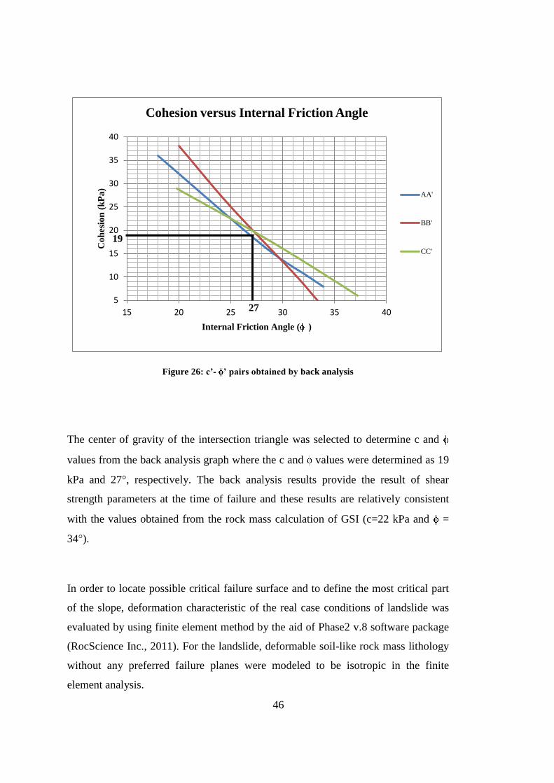
Figure 26: c’- ’ pairs obtained by back analysis ...................................................... 46

Figure 27: Displacement contours of the landslide for present situation ................... 47

Figure 28: Displacement contours of the landslide for partially saturated condition 48

Figure 29: Displacement contours of the landslide for the worst case scenerio ........ 48

Figure 30: Basic structure of fiber cable; a) core, b) cladding, c) coating (Modified

from Hayes, 2006). ..................................................................................................... 50

Figure 31: Light travel path possibilities between two medias (retrieved from

http://farside.ph.utexas.edu/teaching/302l/lectures/node129.html) ........................... 51

Figure 32: Measurement procedure of BOTDA taken from one of the experiments.

The figure at the right hand corner is taken from Ohno et al. (2001) ........................ 57

Figure 33: Brillouin frequency shift due to strain (Ohno et al., 2001)....................... 60

xviii

Figure 34: Optical Time Domain Reflectometer (OTDR) ......................................... 64

Figure 35: Basic structure of the heterecore .............................................................. 65

Figure 36: The utilized fusion splicer (Fujikura FSM 60S) to fuse two cables without

signal loss ................................................................................................................... 66

Figure 37: Cleaver used to cut the fiber cables properly ........................................... 67

Figure 38: Energy loss and displacement relation for the cable pair of 62.5 and

G652D ........................................................................................................................ 68

Figure 39: Energy loss and displacement relation for the cable pair of 62.5 and DSF

.................................................................................................................................... 69

Figure 40: Energy loss and displacement relation for the cable pair of 62.5 and

NZDSF ....................................................................................................................... 69

Figure 41: Representative sketch of laboratory experimental set-up. a) soil barrier

having a height of 20 mm, b) soil-model interface, c) optical fiber cable holes, d)

chain hoist to lift the model up and down in a controlled fashion, e) model feet for

balancing, f) stopper to control mass movement ....................................................... 71

Figure 42: Sieve analysis result for the sand used ..................................................... 72

Figure 43: OTDR sytem measurement in landslide simulator before a movement

based on inclination ................................................................................................... 74

Figure 44: OTDR sytem measurement in landslide simulator after a small movement

based on incination .................................................................................................... 74

Figure 45: Strain changing with respect to displacement .......................................... 77

Figure 46: Initial state of the BOTDA system on the laboratory simulator before

sliding ......................................................................................................................... 78

Figure 47: Appearance of the BOTDA system after given inclination after sliding . 78

Figure 48: Microstrains formed due to changing inclination of the landslide

simulator (red line represents the measurement taken at 10° inclination, green

represents 20° and yellow represents 30° inclination). .............................................. 79

xix

Figure 49: Close up view showing fixing of the cable on a wooden pole ................. 80

Figure 50: A view of opening stage of guidance channels ........................................ 81

Figure 51: Layout of the deployed fiber cables and fixing points (from toe to scarp)

.................................................................................................................................... 82

Figure 52: Layout of the deployed fiber cables and fixing points (from scarp to toe)

.................................................................................................................................... 82

Figure 53: The monitoring unit of the field set up in the container ........................... 83

Figure 54: Landslide geometry shown together with deformation contours and cable

fixing points ............................................................................................................... 84

Figure 55: Baseline measurement of the whole cable ................................................ 85

Figure 56: A close up view of the related portion of the cable along with the

representative daily measurements taken during three days ...................................... 85

Figure A 1: Precipitation graph of December 5, 2010 ............................................. 103

Figure A 2: Precipitation graph of December 10, 2010 ........................................... 104








Figure A 10: Precipitation graph of December 26, 2010 ......................................... 108




1

CHAPTER 1

1. INTRODUCTION

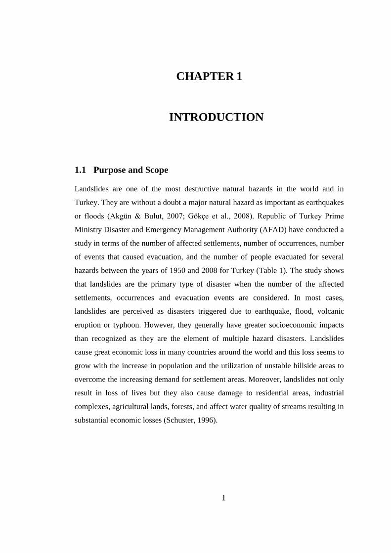
1.1 Purpose and Scope

Landslides are one of the most destructive natural hazards in the world and in

Turkey. They are without a doubt a major natural hazard as important as earthquakes

or floods (Akgün & Bulut, 2007; Gökçe et al., 2008). Republic of Turkey Prime

Ministry Disaster and Emergency Management Authority (AFAD) have conducted a

study in terms of the number of affected settlements, number of occurrences, number

of events that caused evacuation, and the number of people evacuated for several

hazards between the years of 1950 and 2008 for Turkey (Table 1). The study shows

that landslides are the primary type of disaster when the number of the affected

settlements, occurrences and evacuation events are considered. In most cases,

landslides are perceived as disasters triggered due to earthquake, flood, volcanic

eruption or typhoon. However, they generally have greater socioeconomic impacts

than recognized as they are the element of multiple hazard disasters. Landslides

cause great economic loss in many countries around the world and this loss seems to

grow with the increase in population and the utilization of unstable hillside areas to

overcome the increasing demand for settlement areas. Moreover, landslides not only

result in loss of lives but they also cause damage to residential areas, industrial

complexes, agricultural lands, forests, and affect water quality of streams resulting in

substantial economic losses (Schuster, 1996).

2

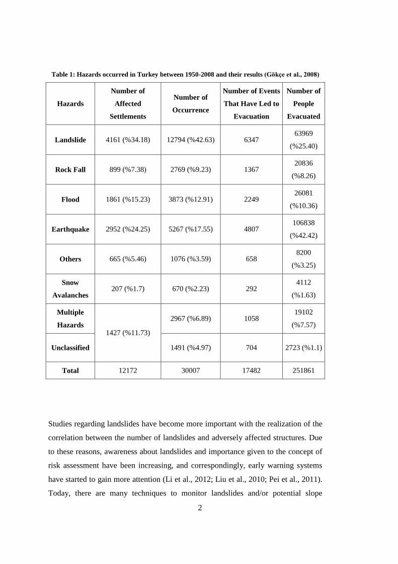
Table 1: Hazards occurred in Turkey between 1950-2008 and their results (Gökçe et al., 2008)

Hazards

Number of

Affected

Settlements

Number of

Occurrence

Number of Events

That Have Led to

Evacuation

Number of

People

Evacuated

Landslide 4161 (%34.18) 12794 (%42.63) 6347 63969

(%25.40)

Rock Fall 899 (%7.38) 2769 (%9.23) 1367 20836

(%8.26)

Flood 1861 (%15.23) 3873 (%12.91) 2249 26081

(%10.36)

Earthquake 2952 (%24.25) 5267 (%17.55) 4807 106838

(%42.42)

Others 665 (%5.46) 1076 (%3.59) 658 8200

(%3.25)

Snow

Avalanches 207 (%1.7) 670 (%2.23) 292

4112

(%1.63)

Multiple

Hazards 1427 (%11.73)

2967 (%6.89) 1058 19102

(%7.57)

Unclassified 1491 (%4.97) 704 2723 (%1.1)

Total 12172 30007 17482 251861

Studies regarding landslides have become more important with the realization of the

correlation between the number of landslides and adversely affected structures. Due

to these reasons, awareness about landslides and importance given to the concept of

risk assessment have been increasing, and correspondingly, early warning systems

have started to gain more attention (Li et al., 2012; Liu et al., 2010; Pei et al., 2011).

Today, there are many techniques to monitor landslides and/or potential slope

3

instabilities and they have their advantages and disadvantages. Inclinometers,

tiltmeters, extensometers, ground based LIDAR, satellite images, and air

photography are examples of techniques used for landslide monitoring (Savvaidis,

2003; Pei et al., 2011). Rather than early warning, these methods are used to detect

subsequent deformation. Among these, optical fiber systems have superiority over

aforementioned systems in terms of their easy and fast data transfer, smaller

dimensions, light weight, sensitivity to strain and temperature change, wide band

range, resistance to environmental and electromagnetic effects, low cost and real

time monitoring properties (Wang et al., 2008; Gupta, 2012; Measures, 2001).

Optical fibers have been used since 1800s but their usage in early warning systems

of landslides is a fairly new concept (Al-Azzawi, 2007).

The purpose of this thesis is to develop an early warning system for landslides that is

related to neither failure mechanism nor lithology type by combining the strain

results collected from fiber cables with displacements on moved masses. For this

purpose, optical fiber systems are preferred due to their superiority in field

conditions and continuous data measurement capabilities. In this study two different

optical fiber systems were experimented with alternative fiber cables and their

competency for a real case landslide area was investigated. Before the field

experiment, systems were tested first in laboratory scale and then in the field. For the

laboratory studies, a landslide simulation model having an inclination mechanism

designed to represent a slope was used. Field application of the system was

performed in a landslide hazard prone region in the Bahçecik Settlement Area in the

Kocaeli Province. The region is located in the south of the city where the topography

is mountainous.

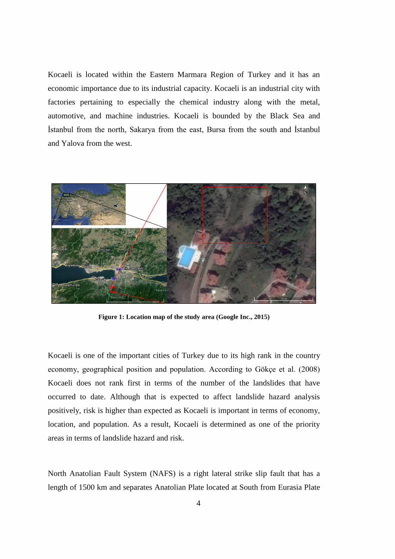
1.2 The Study Area

The study area is located within the borders of Kocaeli Province, Başiskele District,

Bahçecik Settlement Area. The location map of the region is given in Figure 1.

4

Kocaeli is located within the Eastern Marmara Region of Turkey and it has an

economic importance due to its industrial capacity. Kocaeli is an industrial city with

factories pertaining to especially the chemical industry along with the metal,

automotive, and machine industries. Kocaeli is bounded by the Black Sea and

İstanbul from the north, Sakarya from the east, Bursa from the south and İstanbul

and Yalova from the west.

Figure 1: Location map of the study area (Google Inc., 2015)

Kocaeli is one of the important cities of Turkey due to its high rank in the country

economy, geographical position and population. According to Gökçe et al. (2008)

Kocaeli does not rank first in terms of the number of the landslides that have

occurred to date. Although that is expected to affect landslide hazard analysis

positively, risk is higher than expected as Kocaeli is important in terms of economy,

location, and population. As a result, Kocaeli is determined as one of the priority

areas in terms of landslide hazard and risk.

North Anatolian Fault System (NAFS) is a right lateral strike slip fault that has a

length of 1500 km and separates Anatolian Plate located at South from Eurasia Plate

5

located at North.Kocaeli is one of the cities that affected from this fault system.

Therefore, earthquakes should be considered as a major triggering mechanism for

landslides occurred in Kocaeli. Distribution of landslides occurred around the study

area and faults present can be seen in the Figure 2. According to Duman et al. (2006)

landslides reactivated after 1999 İzmit earthquake has an effect on hazard

distribution together with shallow landslides formed.

According to the Republic of Turkey Prime Ministry Disaster and Emergency

Management Authority (AFAD) database, the reported landslides that have occurred

between the years 1960 and 2006 in Kocaeli is given in Table 2 on a district basis.

The numbers given may be uncertain since the table was prepared according to the

reported events (Gökçe et al., 2008).

6

Fig

ure

2:

Dis

trib

uti

on

an

d t

yp

es o

f la

nd

slid

es

tha

t h

av

e o

ccu

rred

an

d f

au

lts

aro

un

d t

he

stu

dy

are

a (

Mo

dif

ied

fro

m L

an

dsl

ide

inte

nsi

ty m

ap

of

Dis

ast

er a

nd

Em

erg

ency

Ma

na

gem

ent

Au

tho

rity

(A

FA

D)

an

d l

an

dsl

ide

inv

ento

ry m

ap

of

Gen

era

l d

irec

tora

te o

f

Min

era

l R

esea

rch

an

d E

xp

lora

tio

n (

MT

A)

7

Table 2: List of the landslides occurred in Kocaeli between 1960-2006 gathered from AFAD

database (Gökçe et al., 2008)

Province District Number of Landslides

Kocaeli

Gebze 12

Merkez 37

Gölcük 12

Kandıra 1

Karamürsel 28

Körfez 2

Yarımca 4

Total Number of Landslides 96

The study area is located at the border of the Başiskele district. Başiskele is not

present in Table 2 since it was founded in 2008, but it lies within the borders of

Merkez where most of the landslides have occurred.

Landslides can be triggered by the intense precipitation, snow melt, earthquakes and

human activities.. The climate and precipitation regime has an effect on landslides.

Also, human activities that include construction of engineering structures like roads

and tunnels have a remarkable impact in Kocaeli. In addition, seismic activity should

be considered due to its proximity to the NAFS.

Apart from the economic importance of Kocaeli, the study area was selected due to

its critical location in terms of landslide risk. In 2010, a landslide occurred and the

region was announced as a hazard prone area by the AFAD in 19.02.2013 because

the landslide was threatening a house that was located in its crown area (Figure 3).

8

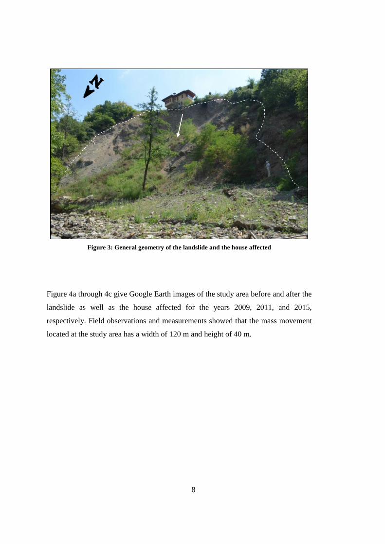
Figure 3: General geometry of the landslide and the house affected

Figure 4a through 4c give Google Earth images of the study area before and after the

landslide as well as the house affected for the years 2009, 2011, and 2015,

respectively. Field observations and measurements showed that the mass movement

located at the study area has a width of 120 m and height of 40 m.

9

Figure 4: Appearance of the study area dated on a) 11.04.2009 (before), b) 05.08.2011 (after), c)

07.05.2015 (after).

a

b

c

10

1.3 Physiography

The catchment basin of the study area trapped by the Gulf of İzmit, İznik Lake and

Sakarya River is formed by the plateaus with varying topographic heights. This area

is geomorphologically differentiated from the Kocaeli Peninsula by the important

topographic heights such as Naldöken (1125 m), Dikmen (702 m), Karlık (892 m)

and especially Kartepe Mountain with an elevation of 1601 meters. Southern parts of

Kocaeli have steeper slopes compared to the northern parts.

On the southern region, volcanic formations are abundant and these volcanic units

composed of andesites and dacites are located within the catchment basin which is

formed by the high mountains and plateaus, and extends through the NE and E

direction until they reach Gölcük and Maşukiye. The regions where volcanic units

located are the areas where events such as landslides and rock falls are expected.

On the southern part, the region between Hersek Delta and the western part of

Gölcük is generally observed as a typical high cliff beach. Some low coasts are also

present around Karamürsel, Ereğli and Yalıdeğirmendere. On the other side of the

bay, on the east and west of this cliffed region, low coasts are observed in larger

areas. On the eastern part, the coast between the Gölcük region and the end of the

gulf of İzmit forms an alignment of transported sediments due to numerous streams.

On the western part, the alluvial sedimentation that forms the Hersek and Laledere

deltas penetrate towards the sea, thus forming the low coast at that region (Kocaeli

Environment and Urbanization Directorate, 2011).

1.3.1 Climate

Kocaeli has a mild climate along the coasts of Black Sea and Gulf of İzmit, and

harsh climate at mountainous regions. It can be said that Kocaeli has a transition

climate between Mediterranean climate and Black Sea climate. Winters are not warm

11

as Mediterranean climate and summers are not as wet as Black Sea climate.

According to the Turkish State Meteorological Service (2014), the annual average

temperature of the last 64 years is 15.0°C. January is the coldest month with an

average temperature of 6.3°C and July is the warmest month with an average

temperature of 23.7°C. The average values of temperature, sunshine duration, rainy

days and precipitation is given in Table 3 on a monthly basis. In addition, the

average monthly temperature and precipitation are presented in Figure 5.

Table 3: Average values of temperature, sunshine duration, and precipitation data in Kocaeli

forthe 1950-2014 period (Turkish State Meteorological Service, 2014).

Value

Aver

age

Tem

per

atu

re

(°C

)

Aver

age

Hig

hes

t

Tem

per

atu

re

(°C

)

Aver

age

Low

est

Tem

per

atu

re

(°C

)

Aver

age

Su

nsh

ine

Du

rati

on

(h

r)

Aver

age

Rain

y D

ays

Mo

nth

ly

Aver

age

Pre

cip

itati

on

(kg/m

2)

Month

January 6.3 9.7 3.3 2.3 17.6 93.2

February 6.7 10.7 3.5 3 15.6 73.3

March 8.6 13.2 4.9 4.6 14.1 73.4

April 13.1 18.5 8.9 5.3 11.9 52.3

May 17.5 23.2 12.9 7.2 9.9 45.4

June 21.7 27.5 16.8 8.6 8.3 52.8

July 23.7 29.5 19.1 9.3 5.8 37.6

August 23.7 29.6 19.2 9.6 5.3 43.6

September 20.4 26.2 16.1 7.1 7.1 52

October 16 20.8 12.5 4.5 11.8 89.9

November 11.9 16.2 8.6 3.4 12.7 81.5

December 8.5 11.9 5.6 2.3 16.4 108

12

Figure 5: Monthly average precipitation and temperature values of Kocaeli between the years

1950-2014 (Turkish State Meteorological Service, 2014)

The annual precipitation distribution of Kocaeli for the years between 1981 and 2010

is shown in Figure 6. Accordingly, the average annual precipitation is 799.5 mm.

The annual precipitation data shows that Kocaeli has received precipitation far over

the average in the years 1981, 1997, and 2010 since 1981 with a nearly 14 years of

recurrence period.

0

5

10

15

20

25

0

20

40

60

80

100

120

1 2 3 4 5 6 7 8 9 10 11 12

Av

era

ge

Tem

per

atu

re (

C

)

Av

era

ge

Pre

cip

ita

tio

n (

mm

)

Monthly Average Precipitation and Temperature

Precipitation Temperature

13

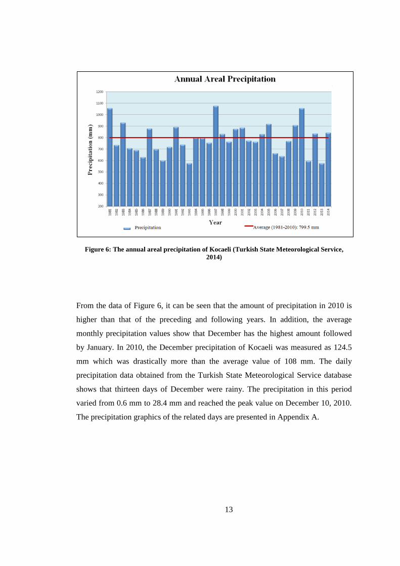
Figure 6: The annual areal precipitation of Kocaeli (Turkish State Meteorological Service,

2014)

From the data of Figure 6, it can be seen that the amount of precipitation in 2010 is

higher than that of the preceding and following years. In addition, the average

monthly precipitation values show that December has the highest amount followed

by January. In 2010, the December precipitation of Kocaeli was measured as 124.5

mm which was drastically more than the average value of 108 mm. The daily

precipitation data obtained from the Turkish State Meteorological Service database

shows that thirteen days of December were rainy. The precipitation in this period

varied from 0.6 mm to 28.4 mm and reached the peak value on December 10, 2010.

The precipitation graphics of the related days are presented in Appendix A.

15

CHAPTER 2

2. GEOLOGICAL SETTING AND ENGINEERING

GEOLOGICAL ASSESSMENT OF THE STUDY

AREA

2.1 Introduction

Kocaeli is surrounded by the topographic heights of the Kocaeli Peninsula on the

north, Armutlu Peninsula on the south and divided into two with the North Anatolian

Fault System (NAFS) by the gulf of İzmit which is an extension of the Marmara Sea

and also the sedimentary basin. This is the main reason why Kocaeli is examined in

three different geomorphological regions which are the Kocaeli peninsula to the

north, Armutlu peninsula to the south and the gulf of İzmit at the center (Kocaeli

Environment and Urbanization Directorate, 2011).

Kocaeli has two geologically important tectonic and structural assemblies. One of

them is the Kocaeli Peninsula containing the İstanbul Paleozoic and the Kocaeli

Triassic units that are located at the north of the gulf of İzmit. According to Şengör

and Görür (1983) the Kocaeli Peninsula was detached from the Moesia platform.

The other assembly is the Armutlu Peninsula which is a part of the Sakarya Zone.

Kocaeli is located on the tectonic assembly called the İstanbul Zone together with

the İstanbul and Kocaeli Peninsulas which are natural extensions of each other. Also,

the gulf of İzmit is located on the east west directional active graben where the North

Anatolian Fault System and the Marmara Graben System are interacted.

16

The Sapanca Lake is located at the eastern part of Kocaeli while Kocaeli and

Armutlu Peninsula are located at the north and south, respectively. The ages of the

formations found in the Kocaeli Peninsula vary between Ordovician and Quaternary

(Gedik et al., 2005) and the units of the Armutlu Peninsula are found in the age

interval of Triassic to Quaternary and dominated by ophiolites and metamorphic

units (Göncüoğlu et al., 1986). There is no chance to observe a continuity,

concordance or correlation since these two units are separated by the North

Anatolian Fault System.

2.2 General Geology and Seismotectonics

The units that outcrop in the Kocaeli Peninsula are composed of Paleozoic and

Permian-Triassic aged allochthonous units, Late Cretaceous-Eocene aged semi-

autochthonous units, and Oligocene-Miocene and Pliocene-Quaternary aged

autochthonous units (Gedik et. al., 2005). There are two Paleozoic aged sequences

and three Permian-Triassic sequences in the Kocaeli Peninsula. The units of these

different aged sequences have originally deposited at various locations and later have

come together as tectonic slices. The Paleozoic units were subjected to tectonic

movements during terrestrial sedimentation and have located in their place as

tectonic slices with transgressive Permian-Triassic units on them. At the Western

Pontides, the age of this placement should be older than Late Jurassic as there are

Late Jurassic-Middle Eocene aged units that rest unconformably on this unit. As the

result of tectonism, faults rather than folded structures were formed in Kocaeli

(Gedik et. al., 2005).

Armutlu Peninsula is situated in NW-Anatolia and composes the western part of the

Pontides. The peninsula is bordered with two main branches of NAFS and it is

approximately located on Mesozoic aged Intra-Pontide Suture. There are several

different units representing the formations starting from Paleozoic outcropped within

the borders of Armutlu Peninsula. Precambrian-Early Paleozoic aged Pamukova

17

Metamorphics compose the basement of the region. Sedimentary and volcano-

sedimentary units that cover the basement are Early Triassic Taşköprü Formation,

Late Paloecene-Middle Eocene aged İncebel Formation, and Eocene aged Sarısu

Formation. Fıstıklı Granodiorite settled during Eocene. At the upper parts, Late

Miocene aged Kılıç Formation, Late Miocene-Early Pliocene aged Yalakdere

Formation, Pleistocene aged marine platform sediments and Quaternary alluviums

(Akartuna, 1968; Göncüoğlu, 1990). These formations can be classified as two main

geological units. One of them is pre-Cenomanian metamorphic basement that made

up of Pamukova Metamorphics and İznik Metamorphics. Other geologic unit is a

non-metamorphic cover with a discontinuous Cenomanian-Pliocene stratigraphic

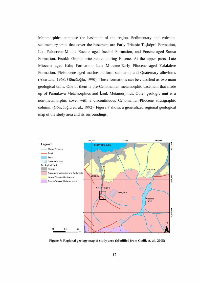
column. (Göncüoğlu et. al., 1992). Figure 7 shows a generalized regional geological

map of the study area and its surroundings.

Figure 7: Regional geology map of study area (Modified from Gedik et. al., 2005)

18

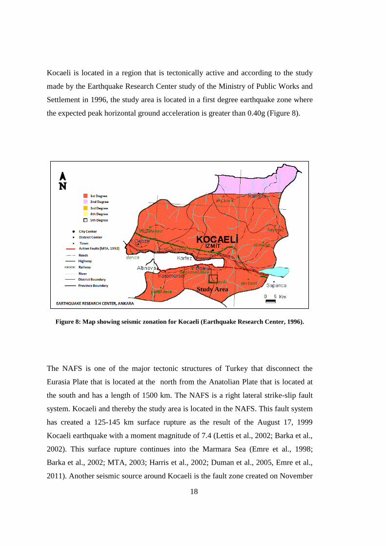
Kocaeli is located in a region that is tectonically active and according to the study

made by the Earthquake Research Center study of the Ministry of Public Works and

Settlement in 1996, the study area is located in a first degree earthquake zone where

the expected peak horizontal ground acceleration is greater than 0.40g (Figure 8).

Figure 8: Map showing seismic zonation for Kocaeli (Earthquake Research Center, 1996).

The NAFS is one of the major tectonic structures of Turkey that disconnect the

Eurasia Plate that is located at the north from the Anatolian Plate that is located at

the south and has a length of 1500 km. The NAFS is a right lateral strike-slip fault

system. Kocaeli and thereby the study area is located in the NAFS. This fault system

has created a 125-145 km surface rupture as the result of the August 17, 1999

Kocaeli earthquake with a moment magnitude of 7.4 (Lettis et al., 2002; Barka et al.,

2002). This surface rupture continues into the Marmara Sea (Emre et al., 1998;

Barka et al., 2002; MTA, 2003; Harris et al., 2002; Duman et al., 2005, Emre et al.,

2011). Another seismic source around Kocaeli is the fault zone created on November

Study Area

19

12, 1999, namely, the Düzce earthquake with moment magnitude of 7.2. This fault

zone has a length of 30 to 45 km (Duman et al., 2005). In addition, there is another

seismic source created by the Abant (May 26, 1957, Ms=7.0) and in Mudurnu (June

22, 1967, Ms=7.1) earthquakes (Ambraseys and Zatopek, 1969). The Mudurnu

earthquake has a 55 km long fault zone that overlaps 25 km of the Abant earthquake

fault zone (Ambraseys and Zatopek, 1969). The 1957 Abant earthquake has a surface

rupture with a length between 30 km (Barka, 1996) and 40 km (Ambraseys and

Zatopek, 1969) that extends between the Abant Lake and Dokurcun. The surface

rupture of the Bolu earthquake (February 1, 1944, Mw=6.8) that occurred near the

study area continues between the Abant Lake and Bayramören (Ketin, 1969; Öztürk

et al., 1985). Major earthquakes around the study region and their focal mechanism

analysis are given by Figure 9.

20

Figure 9: Major earthquakes and focal mechanism analysis within and around the study area

along the NAFS (Cambazoğlu, 2012).

2.2.1 Local geology

The units that outcrop in and around the study area belong to the Sarısu and İncebel

formations. As a consequence, only the details of the characteristics of these

formations will be explained.

The Sarısu formation is a volcano-sedimentary sequence that is commonly observed

in the middle part of the Armutlu Peninsula. It is composed of andesitic lava and

agglomerate. The sequence is found most typically around the Sarısu Village and

outcrops as a northeast-southwest oriented line that divides the peninsula into two

pieces. The sequence contains different lithological order in different places due to

development process of the volcanism. The formation generally starts with a 5-10 m

thick sedimentary level onto metamorphic rocks. This level is composed of

21

conglomerate, mudstone, sandstone and limestone. Conglomerate is made up

ofquartz fragments and is grain supported. Mudstone contains quartz and limestone

fragments. Limestone has the characteristics of packstone with lithoclastic,

bioclastic, nummulite and quartz grains in it. This sedimentation is the 1000 meters

thick part located on top of the basement sequence and is generally composed of

pyroclastic and epiclastic rocks. Pyroclastics have normal, reverse or symmetrical

grading while fine or coarse grained tuff has andesitic tuff and rock fragments in

different sizes. Pyroclastic flow deposits are found in alternation with symmetrical

graded or ungraded lahar deposits. Some levels of the sequence contain huge

andesite blocks and pebbles of epiclastic deposits that probably have the

characteristics of beach conglomerate. Lava flows within the sequence that are found

at the upper levels and have a thickness of 5 meters show an alternation with

pyroclastic rocks. Lava flows are composed of andesitic volcanic rocks with

plagioclase, pyroxene and hornblende phenocrysts. Tuffs contain plagioclase, glass

and fluidal textured volcanic fragments within a glass matrix. Lahar deposits which

formed as a result of pyroclastic flow having normal or symmetrical grading have

developed irregular unconformity planes by scratching the flow surfaces. All this

sequence is cut by basalt dykes that are observed especially in the upper levels.

Basalts have augite and plagioclase and appear to be much fresher than andesite.

The Sarısu formation is located on metamorphic rocks with a thin level of basal

conglomerate, and has a tuff and sandstone alternation at its contact with the İncebel

flysch. Limestone and sandstone specimens located at the lowest level of the

volcanic sequence and metamorphic unconformity shows that the sequence

developed starting from Lutetian (Erendil et. al., 1991).

The İncebel Formation is a Paleocene-Eocene aged formation seen generally at the

south of Karamürsel. The formation unconformably covers the metamorphic units

and forms a 3000 m thick sequence in the İncebel Village and dips towards

northwest. The İncebel formation starts with a basal conglomerate layer composed of

22

pebbles of the units that overlay and its color is observed to be purple, gray or yellow

according to underlying unit. The İncebel formation is generally composed of a

flysch sequence of sandstone, mudstone, marl, and conglomerate. However, it can

contain volcanic lithologies, namely light colored tuffs and andesitic agglomerate in

the upper parts of the sequence. Due to the presence of this volcanic level, the

İncebel formation is interpreted to occur in alternation with the Sarısu formation

(Göncüoğlu et al., 1992).

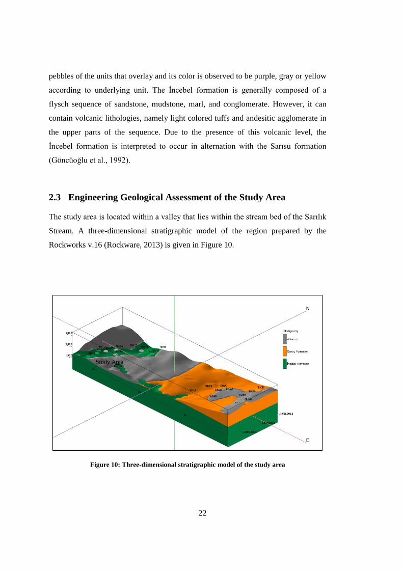
2.3 Engineering Geological Assessment of the Study Area

The study area is located within a valley that lies within the stream bed of the Sarılık

Stream. A three-dimensional stratigraphic model of the region prepared by the

Rockworks v.16 (Rockware, 2013) is given in Figure 10.

Figure 10: Three-dimensional stratigraphic model of the study area

Study Area

23

A field study conducted in order to understand the general geological and

engineering geological properties of the region revealed that the lithology in the

study area consists of an alternation of sandstone and marl. Figure 11 shows a close-

up view of the lithology. According to the field observations, this unit is correlates

with the Paleocene-Eocene aged İncebel formation.

Figure 11: A close-up view of the Ġncebel formation

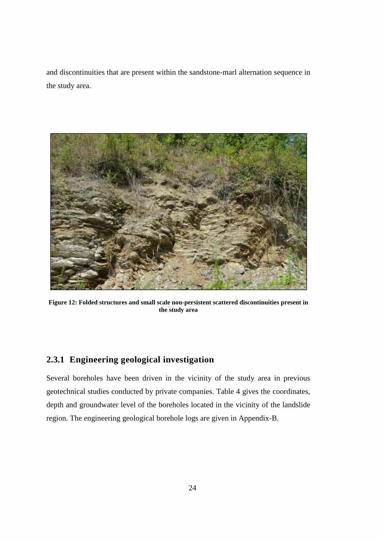
The sandstone marl alternation sequence contains scattered and non-persistent

discontinuity sets. Small scale folds are observed in the field. As explained in

Section 2.2, the study area is located within a tectonically active region, or in other

words, in a shear zone. Figure 12 shows a view of the folded and sheared structures

24

and discontinuities that are present within the sandstone-marl alternation sequence in

the study area.

Figure 12: Folded structures and small scale non-persistent scattered discontinuities present in

the study area

2.3.1 Engineering geological investigation

Several boreholes have been driven in the vicinity of the study area in previous

geotechnical studies conducted by private companies. Table 4 gives the coordinates,

depth and groundwater level of the boreholes located in the vicinity of the landslide

region. The engineering geological borehole logs are given in Appendix-B.

25

Table 4: The coordinates, depth and groundwater level of the boreholes

Borehole

Number X Y Z

Depth

(m)

Groundwater

Depth from

Surface (m)

SK5 492103.631 4503627.344 209.585 12.00 -

SK9 491609.017 4503564.437 136.944 12.00 3.00

SK10 491623.3 4503456.893 155.678 12.00 -

SK11 491624.15 4503416.77 159.929 12.00 -

SK12 491484.971 4503483.266 118.705 18.00 3.00

SK13 491402.697 4503446.256 119.547 18.00 3.00

SK14 491336.562 4503354.646 122.674 18.00 3.00

SK15 491287.681 4503189.871 145.695 10.00 3.00

SK16 491295.539 4503084.843 158.755 12.00 -

SK17 491313.861 4503264.014 138.109 21.00 4.00

SK18 491404.1 4503277.226 138.26 21.00 4.00

SK19 491256.442 4503243.465 133.987 10.00 4.00

SK21 492362.247 4503265.973 209.223 13.00 -

SK22 492295.662 4503154.601 192.723 12.00 9.00

The engineering geological characterization of the studied region was accomplished

with 201 m of boring data resulting from a total of 14 boreholes. Note that these

boring data were obtained from adjacent to the landslide location. According to the

boring results, there is a 1-2 m thick soil cover on the upper levels of the İncebel

formation and this soil cover is underlain by a sandstone siltstone marl sequence.

The groundwater was encountered on nine of the fourteen boreholes at a depth

generally varying from 3 to 4 m from the ground surface.

26

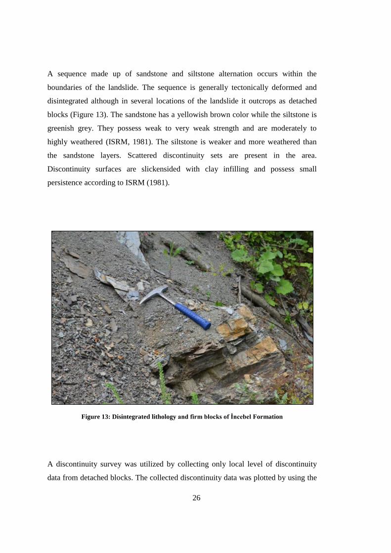
A sequence made up of sandstone and siltstone alternation occurs within the

boundaries of the landslide. The sequence is generally tectonically deformed and

disintegrated although in several locations of the landslide it outcrops as detached

blocks (Figure 13). The sandstone has a yellowish brown color while the siltstone is

greenish grey. They possess weak to very weak strength and are moderately to

highly weathered (ISRM, 1981). The siltstone is weaker and more weathered than

the sandstone layers. Scattered discontinuity sets are present in the area.

Discontinuity surfaces are slickensided with clay infilling and possess small

persistence according to ISRM (1981).

Figure 13: Disintegrated lithology and firm blocks of Ġncebel Formation

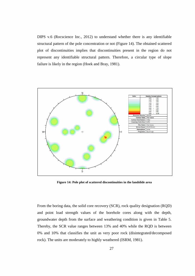
A discontinuity survey was utilized by collecting only local level of discontinuity

data from detached blocks. The collected discontinuity data was plotted by using the

27

DIPS v.6 (Rocscience Inc., 2012) to understand whether there is any identifiable

structural pattern of the pole concentration or not (Figure 14). The obtained scattered

plot of discontinuities implies that discontinuities present in the region do not

represent any identifiable structural pattern. Therefore, a circular type of slope

failure is likely in the region (Hoek and Bray, 1981).

Figure 14: Pole plot of scattered discontinuities in the landslide area

From the boring data, the solid core recovery (SCR), rock quality designation (RQD)

and point load strength values of the borehole cores along with the depth,

groundwater depth from the surface and weathering condition is given in Table 5.

Thereby, the SCR value ranges between 13% and 40% while the RQD is between

0% and 10% that classifies the unit as very poor rock (disintegrated/decomposed

rock). The units are moderately to highly weathered (ISRM, 1981).

28

Table 5: Engineering geological characteristics gathered from borehole data

Borehole Depth

(m)

Ground Water Point Load

Strength SCR

(%) RQD (%)

Weathering

Degree Depth From

Surface (m) Index (MPa)

SK5 12 - - 13 0 Moderate to

high

SK9 12 3 5.13 20 0 Moderate to

high

SK10 12 - 0.27 21 3 Moderate to

high

SK11 12 - 0.32 25 10 Moderate

SK12 18 3 2.81 40 10 Moderate

SK13 18 3 0.45 24 1 Moderate to

high

SK14 18 3 4.98 22 3 Moderate

SK15 10 3 2.44 15 2 Moderate to

high

SK16 12 - - 17 0 Moderate to

high

SK17 21 4 2.71 17 0 Moderate to

high

SK18 21 4 4.31 18 0 Moderate to

high

SK19 10 4 3.54 18 2 Moderate to

high

SK21 13 - 0.1 20 4 Moderate to

high

SK22 12 9 - 1 0 Moderate to

high

Since the project site is located in a tectonically deformed zone and since the pole

plot distribution shows scattering, the rock mass could be treated as an irregularly

jointed, highly foliated and very deformable soil-like material, from an engineering

geology point of view.

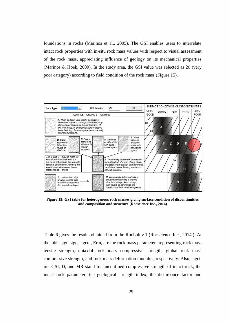
The Geological Strength Index (GSI) is a system of a rock mass characterization

developed with the Hoek-Brown failure criterion to meet the need for a reliable input

data into numerical analyses and analytic solutions for designing tunnels, slopes or

29

foundations in rocks (Marinos et al., 2005). The GSI enables users to interrelate

intact rock properties with in-situ rock mass values with respect to visual assessment

of the rock mass, appreciating influence of geology on its mechanical properties

(Marinos & Hoek, 2000). In the study area, the GSI value was selected as 20 (very

poor category) according to field condition of the rock mass (Figure 15).

Figure 15: GSI table for heterogenous rock masses giving surface condition of discontinuities

and composition and structure (Rocscience Inc., 2014)

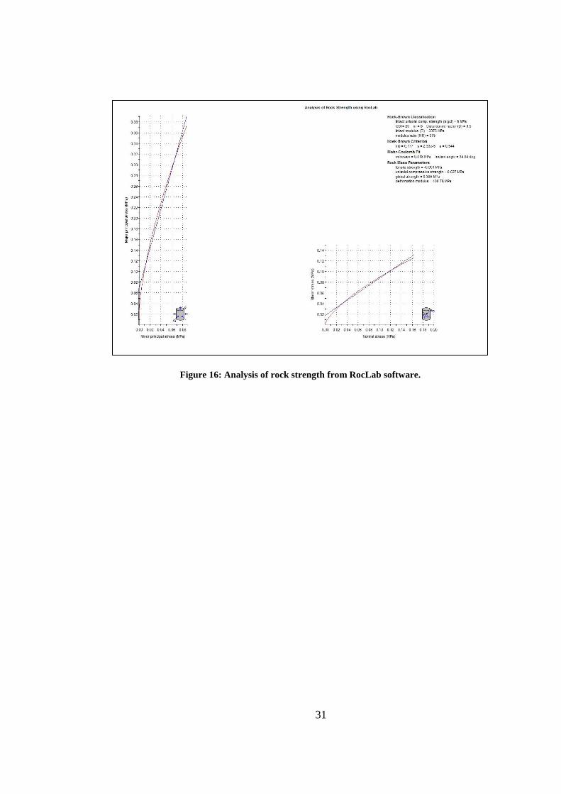
Table 6 gives the results obtained from the RocLab v.1 (Rocscience Inc., 2014.). At

the table sigt, sigc, sigcm, Erm, are the rock mass parameters representing rock mass

tensile strength, uniaxial rock mass compressive strength, global rock mass

compressive strength, and rock mass deformation modulus, respectively. Also, sigci,

mi, GSI, D, and MR stand for unconfined compressive strength of intact rock, the

intact rock parameter, the geological strength index, the disturbance factor and

30

modulus ratio. In addition, mb is a reduced value of material constant mi, and s, and a

are Hoek Brown constants.

Table 6: Geomechanical rock mass paramaters from the RocLab software (Rocscience Inc.,

2014)

Rock Mass Parameters Hoek Brown Classification

sigt -0.001 MPa sigci 9 MPa

sigc 0.027 MPa GSI 20

sigcm 0.410 MPa mi 9

Erm 100.78 MPa D 0.5

Failure Envelope Range MR 375

Application Slopes Hoek Brown Criterion

Mohr-Coulomb Fit mb 0.199

c 0.022 MPa s 2.33e-5

33.88⁰ a 0.544

GSI system applied by using field study observations and measurements was

resulted with a cohesion (c) value of 22 kPa and internal friction angle ( ) value of

34 degrees. Figure 16 shows the rock strength analysis results of the GSI system

from RocLab software.

31

Figure 16: Analysis of rock strength from RocLab software.

33

CHAPTER 3

3. SLOPE STABILITY

3.1 Introduction

Cruden (1991) defines landslide as "the movement of a mass of rock, debris or earth

down a slope."

The purpose of slope stability analysis is to reach safe and economic design of any

related structure such as excavations, embankments, earth dams, and landfills. Slope

stability analysis contains both identification of geological, material, environmental

and economic parameters and understanding of nature, magnitude and frequency.

Slope stability analysis aims to:

Understand development and form of a mass movement

Analyze short-term and long-term stability

Assess landslide possibility

Find failure mechanism and effect of environmental factors

Redesign with back analysis for planning, design and remediation

Examine seismic loading effect.

Slope stability analysis takes into account factors such as topography, geology,

material properties, and neutrality. A slope can be either a natural slope or a man-

made engineered slope. Natural slopes are those formed as a result of landscapes and

these could be triggered by changes in topography, groundwater level, stress,

34

strength as well as seismicity and weathering. Engineering slopes originates from

man-made structures like embankments, cut slopes and retaining walls (Abramson et

al., 2002).

Slope movement occurs as a result of increase in shear stress or decrease in shear

strength of the rock mass. Shear stress of a slope increases due to removal of

support, overloading, transitory effects, removal of material from toe of the slope,

and increase in lateral pressure. Reduction of shear strength is related to change in

material properties, due to changes of weathering, pore pressure, and structural

changes. In addition, preexisting discontinuities found in a slope region such as

faults, bedding planes, foliations, cleavages, sheared zones, and dikes weaken the

residual soil and the weathered bedrock (Abramson et al., 2002).

3.2 Modes of Failure

Varnes (1978) classifies landslides according to type of movement and type of

material. Simplified version of Varnes classification is given in Table 7. Based on

this table any landslide could be identified with two criteria: the first one describes

the material and the second one describes the type of movement.

35

Table 7: Modes of slope failure (Varnes, 1978).

Type of Movement

Type of Material

Bedrock

Engineering Soils

Predominantly

Coarse

Predominantly

Fine

Fall Rock Fall Debris Fall Earth Fall

Topple Rock Topple Debris Topple Earth Topple

Slide Rotational

Rock Slide Debris Slide Earth Slide

Translational

Spread Rock Spread Debris Spread Earth Spread

Flow Rock Flow Debris Flow Earth Flow

Complex Combination of two or more principal types of movement

According to Varnes’ classification, material composing a landslide can be rock or

soil. Soil is further divided into two groups as debris and earth. Rock corresponds to

a firm mass that was intact before the movement while soil could be described as an

aggregate of solid materials like minerals and rocks that formed in situ due to the

weathering of rock or that are allochthonous (i.e., transported from somewhere else).

Soil has two subgroups based on particle size. 1) soil mass is called earth if 80% or

more of the particles are smaller than sand-size particles (2mm) and 2) called debris

if 20% to 80% of material are larger than 2mm. (Cruden and Varnes, 1996).

3.3 Methods of Slope Stability Analysis

Gathering information about engineering properties of material present at landslide

area is a basic step of slope design. There are numerous analyses methods but none

of them are applicable for all slope failures as the internal stress state of the region

36

and the stress strain relation before and after a mass movement could not be defined

with certainty. Today most of the methods use limit equilibrium analysis in which

failure is assumed to be incipient with a safety factor of one. There are other

complex methods such as finite element method (FEM) and boundary element

method (BEM) which require a complete model of subsoils and extensive laboratory

tests to determine soil’s constitutive parameters. Due to its easy implementation limit

equilibrium methods are preferred although they neglect stress-deformation

increments or decrements of slope masses. Conventional slope stability analysis is

based on the limit equilibrium concept and it gives a factor of safety which is a

unitless measure of stability. Limit equilibrium formulation gives statistically

indeterminate solution, so it is not possible to compare it with a closed form solution

directly. However, factor of safeties obtained from different methods could be

compared (Abramson et al., 2002).

Moment equilibrium is not satisfied by Janbu’s simplified method while Bishop’s

simplified method does not satisfy horizontal force equilibrium. FS calculated by

these two methods are 15% percent different than Spencer’s and the Morgenstern-

Price method which consider complete force and moment equilibrium. Bishop’s

simplified method for circular failure surface gives more or less the same result

(difference is less than 5%) with more rigorous methods. But, Janbu’s simplified

method is used for noncircular failures and it underestimates the factor of safety as

much as 30% compared to more rigorous methods. The methods which satisfy

complete equilibrium such as Janbu’s rigorous, Spencer or Morgenstern-Price

methods are more complex (Abramson et al., 2002). Morgenstern-Price method is

preferred as the method is applicable to both circular and noncircular failures and it

satisfies force equilibrium in x and y and moment equilibrium to determine more

realistic results. In this study, the limit equilibrium analysis was established by using

this method.

37

One of the main purposes of this thesis study was to assess the deformation analysis

by using finite element method and compare these data with the field monitoring

results. In order to implement a finite element model rock mass strength parameters

are needed (i.e., shear strength and elastic parameters). Additionally, geotechnical

laboratory test results that were mentioned previously provide the index parameters

of the intact rock, but the case dealt in the field is related to rock mass properties.

GIS was used to overcome the data need and then, back analysis was conducted to

determine shear strength parameters of the material. After mobilized shear strength

parameters are determined by back analysis, it is important to reach deformation

results that will be the correlative parameter with monitoring results.

3.4 Back Analysis

Stability analysis is performed to reach a factor of safety for slopes with known

parameters in general, but they can be used to find shear strength values of a failed

slope. In order to establish a back analysis, the slope stability analysis needs to be

performed in a reverse order by a known factor of safety value; assumed 1 at the

time of failure. This reverse order analysis is called back analysis (Bromhead, 1992).

Back analysis procedure develops an analytical model of a slope failed or about to

fail and the model contains five components.

1. Landslide geometry with ground surface, slip surface, and material

boundaries

2. Pore water pressures on the sliding surface at the time of failure (required for

effective stress analysis)

3. External loads acting on the slope at the time of failure

4. Unit weights of the materials involved in the landslide

5. Strength of materials along the failure surface.

38

In general, the first four parameters could be evaluated by field and laboratory

studies with certain accuracy and the fifth component could be obtained by back

analysis by assuming that the factor of safety equals 1. Back analysis provides

information about the shear strength parameters of a slope for future design that

could not be reached by conventional laboratory tests (Abramson et al., 2002).

3.5 Mechanism of the Landslide in the Study Area

The data gathered showed that the units forming the landslide are classified as poor

and very deformable soil-like lithology. It is known that the landslide occurred on

December 10, 2010. There was heavy precipitation before and during the day the

landslide occurred and the water level of the Sarılık stream increased with the

precipitation that led to flooding.

Also, there was no sign of a seismic activity within a 100 km circle around the study

area during the period of 01.01.2010 and 31.01.2011 according to the Kandilli

Observatory and Earthquake Research Institute (KOERI) database (Figure 17). The

data regarding the earthquakes that occurred in a 100 km circumference of the region

is given in Appendix C. Hence, it could be concluded that the landslide was triggered

by intense precipitation due heavy rainfall that caused the deformable soil-like

landslide material to saturate and the increase of water flow at the toe of the slope

leading to a landslide phenomenon.

39

Figure 17: Earthquake catalogue of 2010 (KOERI http://www.koeri.boun.edu.tr/sismo/2/en/)

Deformational characteristics are important for characterizing the landslide and real

case rock mass parameters are required to calculate the deformations. Hence the

landslide has been modeled by finite element analysis that requires rock mass

parameters (i.e., shear strength and elastic parameters) and these parameters could be

calculated by back analysis along with the GSI results. Therefore, at first a back

analysis was implemented to calculate the mobilized shear strength parameters of the

landslide, and then the area was modelled through finite element analysis. To

determine the landslide geometry prior to failure, a digital elevation model of the

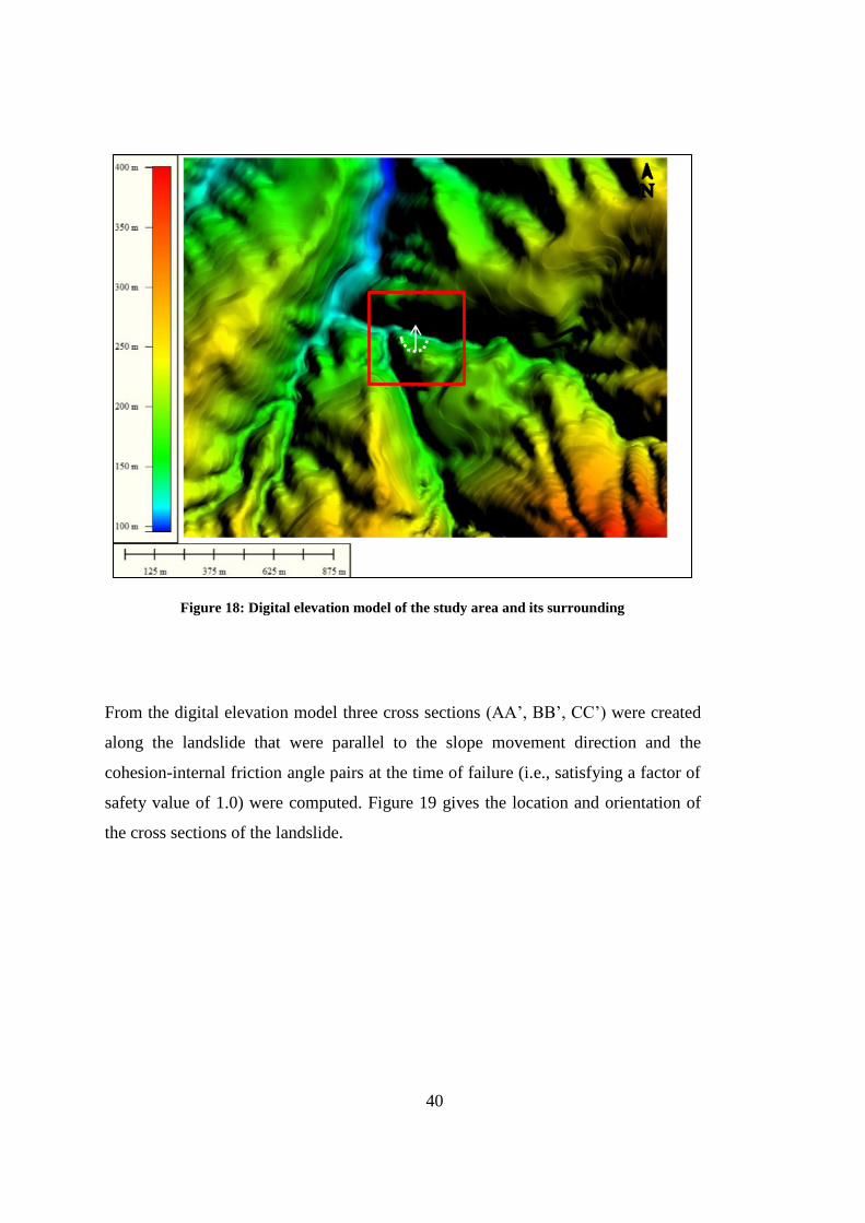
area was created from the topographical contours (Figure 18).

Study Area

40

Figure 18: Digital elevation model of the study area and its surrounding

From the digital elevation model three cross sections (AA’, BB’, CC’) were created

along the landslide that were parallel to the slope movement direction and the

cohesion-internal friction angle pairs at the time of failure (i.e., satisfying a factor of

safety value of 1.0) were computed. Figure 19 gives the location and orientation of

the cross sections of the landslide.

41

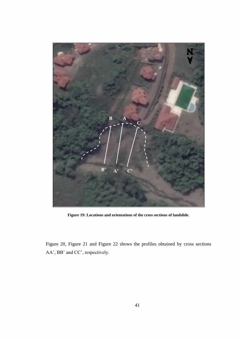
Figure 19: Locations and orientations of the cross sections of landslide.

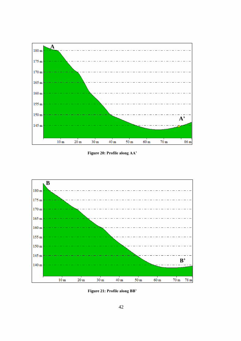
Figure 20, Figure 21 and Figure 22 shows the profiles obtained by cross sections

AA’, BB’ and CC’, respectively.

A

A’ B’ C’

B C

42

Figure 20: Profile along AA’

Figure 21: Profile along BB’

A

A’

B

B’

43

Figure 22: Profile along CC’

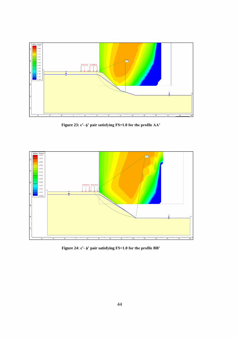
Once the cross sections were created, the back analysis was performed through limit

equilibrium solution by the Morgenstern-Price method using the Slide v.6 software

(Rocscience Inc., 2010). A fully saturated mass (representing heavy rainfall and

flooding conditions) together with a 30 kPa of surcharge to represent the surcharge

of the houses that are located in and behind the crown area (two-storey residential

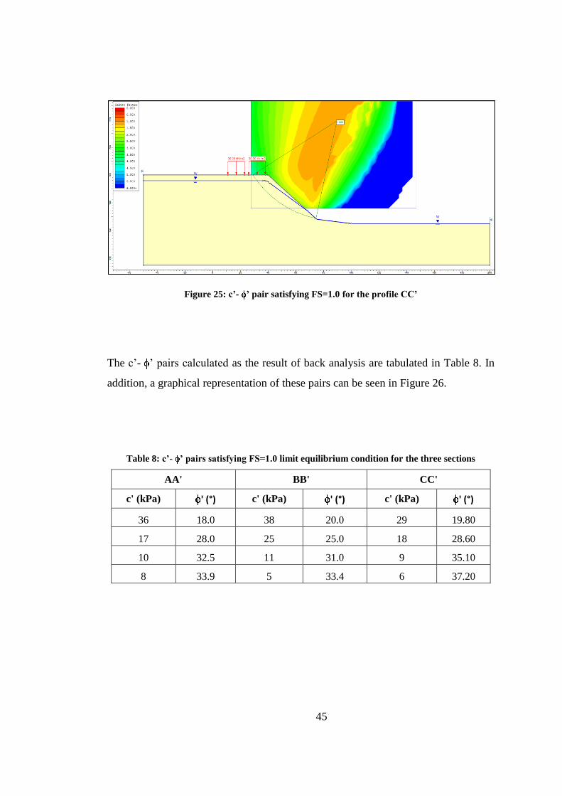
buildings). Figure 23, Figure 24 and Figure 25 represent the back calculated results

of the limit equilibrium analyses of the cross-sections AA’, BB’ and CC’.

C’

C

44

Figure 23: c’- ’ pair satisfying FS=1.0 for the profile AA’

Figure 24: c’- ’ pair satisfying FS=1.0 for the profile BB’

45

Figure 25: c’- ’ pair satisfying FS=1.0 for the profile CC’

The c’- ’ pairs calculated as the result of back analysis are tabulated in Table 8. In

addition, a graphical representation of these pairs can be seen in Figure 26.

Table 8: c’- ’ pairs satisfying FS=1.0 limit equilibrium condition for the three sections

AA' BB' CC'

c' (kPa) ' (°) c' (kPa) ' (°) c' (kPa) ' (°)

36 18.0 38 20.0 29 19.80

17 28.0 25 25.0 18 28.60

10 32.5 11 31.0 9 35.10

8 33.9 5 33.4 6 37.20

46

Figure 26: c’- ’ pairs obtained by back analysis

The center of gravity of the intersection triangle was selected to determine c and

values from the back analysis graph where the c and values were determined as 19

kPa and 27°, respectively. The back analysis results provide the result of shear

strength parameters at the time of failure and these results are relatively consistent

with the values obtained from the rock mass calculation of GSI (c=22 kPa and =

34°).

In order to locate possible critical failure surface and to define the most critical part

of the slope, deformation characteristic of the real case conditions of landslide was

evaluated by using finite element method by the aid of Phase2 v.8 software package

(RocScience Inc., 2011). For the landslide, deformable soil-like rock mass lithology

without any preferred failure planes were modeled to be isotropic in the finite

element analysis.

5

10

15

20

25

30

35

40

15 20 25 30 35 40

Co

hes

ion

(k

Pa

)

Internal Friction Angle (

)

Cohesion versus Internal Friction Angle

AA'

BB'

CC'

27

19

47

In order to understand the effect of groundwater in the landslide area, sensitivity

analyses were performed with different scenario levels of groundwater. Figure 27

shows the deformation contours obtained by the finite element solution for the

present case groundwater situation. Figure 28 displays the deformation contours for a

partly saturated groundwater condition can be possible during a heavy rainfall

precipitation. Lastly, Figure 29 gives the deformation contours for fully saturated

condition that can be represented the worst case scenerio.

Figure 27: Displacement contours of the landslide for present situation

These different scenarios show that the larger deformations generally locate at the

middle and toe part of the slope and deformation value near the surface of the

landslide ranges from 7.20 mm to 9.90 mm (top to bottom) in the present case while

it is in between 7.20 mm and 10.5 mm (top to bottom) for partially saturated and

between 7.80 mm and 10.8 mm (top to bottom) for fully saturated model. Although

these analyses performed to determine critical failure surface in terms of

48

deformation, the results will be compared with the field monitoring data in the

following chapters.

Figure 28: Displacement contours of the landslide for partially saturated condition

Figure 29: Displacement contours of the landslide for the worst case scenerio

49

CHAPTER 4

4. LANDSLIDE AND SLOPE MONITORING

SYSTEM

4.1 Introduction

Although the history of optical fiber dates back to the 1700s with the invention of

optical telegraph, it is being used in communication systems since 1977 (Al-Azzawi,

2007). Today optical fiber systems have many different areas of usage ranging from

telecommunication to structural health monitoring, from monitoring of petroleum

and natural gas pipelines to early warning systems of engineering structures. Some

examples of these are telecommunication services such as cable television, high-

speed internet, wireless transition, remote monitoring, surveillance; military

application such as communication, command and control of ships and aircrafts,

links for satellite ground stations; monitoring and sensing of engineering structures,

gas and DNA sensors; lighting systems. Having such a large area of applications,

requirements for fiber cables can be coated according to different requirements

(temperature, chemicals or radiation resistant) to make them resistant to application

environment.

4.2 Optical Fibers

An optical fiber is a transmission medium that conducts the light from cable’s one

end to another in order to transfer it along a long distance. Optical fibers are thin

cables composed of core and cladding, and their material is generally plastic or glass

(silica). Fiber optic cables are made up of two main parts as core and cladding that

covers the core. In addition to these two layers, a coating is coiled to protect the core

and the cladding. Figure 30 shows the basic structure of an optical fiber cable.

50

Figure 30: Basic structure of fiber cable; a) core, b) cladding, c) coating (Modified from Hayes,

2006).

Light’s transmission through a fiber is based on the Snell’s law (Snellius, 1621).

Snell’s equation explaining the relation between index of refraction and incidence

angle of light is given by Equation 1. Also, critical angle calculation is given by

Equation 2. Critical angle is a parameter related to total internal reflection. As the

index of refraction of the core is slightly higher than that of the cladding, light

launched through the cable travels within the core. This phenomenon is called total

internal reflection (TIR). Figure 31 represents the light traveling between two

mediums and shows the structure of the total internal reflection.

(1)

(2)

a

b

c

9 μ

m

12

5 μ

m

25

0 μ

m

51

Figure 31: Light travel path possibilities between two medias (retrieved from

http://farside.ph.utexas.edu/teaching/302l/lectures/node129.html)

In order to obtain data through a fiber optic system, the fiber cable itself can be used

or sensitive regions, namely sensors can be deployed within the cable with a certain

interval for the desired application. Optical fiber sensors can be classified into three

groups as point, distributed, and quasi-distributed sensors. Point sensors measure

changes from certain points on fiber cable. Conversely, distributed sensors make

measurements along the cable, so they are capable of representing distribution of

spatial changes. These types of sensors use Raman and Brillouin scattering

principles. Quasi-distributed sensors are somewhere between point and distributed

sensors; in such a way that information comes from certain points on the cable but

data acquisition occurs along the cable (Grattan et al., 2000). Selection of sensors

depends on the parameter to be measured (deformation, temperature, moisture, etc.),

utilized device, and desired measurement sensitivity.

52

4.2.1 Classification of optical fibers

Although optical fibers are classified generally into two main groups as multimode

and single mode cables they can be classified according to their production material,

structure, function and performance.

According to the manufacturing materials, optical fibers can be classified generally

as; silica fiber, compound glass fiber, plastic optical fiber, infrared fiber and crystal

fiber. The most common materials used for fiber cable manufacturing are silica

(SiO2) and composite glass fiber composed of silicate, phosphate and fluorite.

According to their structure, fibers are divided into step-index fibers, graded index

fibers (GRIN), double cladding fibers (DCF), photonic crystal fibers (PCF),

polarization maintaining fibers (PMF) and large aperture fibers. According to the

function and performance, fibers are grouped into two categories as single mode

fiber (SMF) and multimode fiber (MMF) (Fang et al., 2012). A single mode fiber has

a core diameter ranging from 4 µm to 10 µm and this core diameter is small when

compared to the wavelength of light. Due to the small core diameter, light could

travel only in a single path or mode within a single mode fiber. On the other hand,

multimode fibers have larger core diameter ranging from 25 µm to 150 µm allowing

light to travel in many paths or modes (Iten, 2011).

4.2.2 Advantages of optical fibers

Optical fibers have superiority over conventional methods in terms of several

characteristics, namely easy and fast data transfer, small diameter, light weight,

sensitivity to strain and temperature change, wide band range, resistance to

environmental and electromagnetic effects, and low cost (Wang et al., 2008; Gupta,

2012; Measures, 2001).

53

Powers (1997) gives the advantages of fiber optic as wide bandwidth, light weight

and small size, immunity to electromagnetic interference, lack of electromagnetic

interference crosstalk between channels, lack of sparking, compatibility with solid

state sources, and low cost.

Bandwidth is the measure of the frequency range width of a medium that depends on

carrier frequency. Optical fibers have higher frequencies than other methods which

make them superior. Bandwidth of a fiber cable can be of several THz and this

allows transfer of data from many different sources, so that they are applicable to a

wide range of fields. Fiber optics have small dimensions and low density that allow

them to be light and small in size. This property is an advantage in field application

especially when the considered length is long. These physical characteristics result in

an ease of the transportation of the cable since it is possible to install the cable in

smaller areas. Electromagnetic interference is a problem for data transfer and it is

almost impossible to avoid in electric related features and applications. Optical fiber

technology is immune to electromagnetic interference which is why they can be

implemented anywhere without being affected from electromagnetism. Furthermore,

optical fiber cables are applicable to hazardous areas as they do not spark. Due to

this characteristic, they can be safely used for any application without changing the

application route. This property of optical fiber cables allows them to be utilized in

flammable and toxic gas environments. Optical fibers are compatible with modern

electronic components as a result of their material and dimensions (Powers, 1997).

The main superiority of the optical fibers are their capability to transport more data

to in longer distances faster than any other medium (Hayes, 2006). Electromagnetic

radiation does not affect optical fibers, thus allowing data transfer with smaller noise

and error. Furthermore, unlike metallic conductors, utilization of fiber optics in the

fields of sensor applications, medical applications, industrial applications, subject

illumination, and image transport is possible (Hayes, 2006).

54

4.3 The Utilized Optical Fiber System

Today, optical fiber systems are being used to monitor buildings, bridges, tunnels,

dams, slopes, pipelines, gas tanks, and ships for detection of changes in acceleration,

chemicals/gases, color, distance, force, humidity, magnetic/electric field,

movement/displacement, linear and angular position, pressure, and radiation (Altuğ,

2007). It is possible to detect these changes as chemical and physical properties

affecting the intensity, scattering and polarization of light traveling within the fiber.

These measurements are achieved by analyzing the amplitude, frequency, phase and

polarization of the backscattered light.

Scattering is the dispersion and loss of incident light due to hitting any unexpected

material such as irregularities caused from fiber production. There are three major

scatter types concerning optical fibers; Rayleigh, Brillouin, and Raman. Rayleigh

scattering is a linear scattering while Brillouin and Raman scatterings are nonlinear

(Yücel et al., 2014). Rayleigh scattering is the result of very small irregularities

within the fiber that have smaller dimensions than the wavelength of transmitted

light. These irregularities show their effect in the refractive index as fluctuations. As

a consequence, Rayleigh scattering occurs in almost all directions. Brillouin

scattering could be identified as an interaction between acoustic wave and pumped

wave. It is revealed as a result of the interaction of pumped light moving within the

fiber and acoustic waves formed thermally and spontaneously. Raman scattering is

the product of interaction between the light launched to fiber and molecular vibration

modes of the medium. It could be described as scattering of light from phonons

(Mafang, 2011).

An optical fiber system is not composed of only fiber cables but it also contains a

device that launches light into the cable and collects backscattered light and in some

cases sensitive regions called sensors. There are several different types of devices

55

used with an optical fiber system. During this study, time domain reflectometry was

used as a source and receiver.

4.3.1 Optical fiber system utilized with OTDR

Time domain reflectometry is a phenomenon based on a deformation on a cable due

to any effect, and ground motion in the case of a landslide. The motion is determined

by monitoring the pulsed light’s backscattering time (Yan et al., 2010). An Optical

Time Domain Reflectometer (OTDR) is one of these devices that is invented by

Barnoski & Jensen (1976). Its purpose is to detect, locate and measure events at any

location on a fiber array. An OTDR sends the light to cable and collects

backscattered light. By using amplitude, the return time of backscattered light can be

determined (Fang et al., 2012). An OTDR gives the location of reflection that

corresponds to a change in a cable due to any effect in terms of decibel (dB).

Decibel is a logarithmic unit and is used for the expression of the ratio of physical

quantities. In the earlier years, power was measured in terms of milliwatts and loss

was measured in decibels (dB). Over the years, dB started to be used for all

measurements for convenience (Hayes, 2006). A decibel is a unit used for the

comparison of power units and could be defined as the ratio of the input optical

power to the output optical power (measured) for a certain wavelength. The number

of decibels is defined with Equation 3 (Mohammed et al., 2013).

(3)

56

As the equation implies, dB is a logarithmic scale and every10 dB represents 10

times ratio. Therefore, 10 dB means a ratio of 10 times, 20 dB means a ratio of 100

times, 30 dB means a ratio of 1000 times and so on (Hayes, 2006).

4.3.2 Optical fiber system utilized with BOTDA

A Brillouin Optical Time Domain Analyzer (BOTDA) was the second device used in

this study. It is again a distributed optical fiber sensor but it works with the Brillouin

scattering principle. These systems are named as time domain systems as they use

time interval between launched and backscattered light similar to the Optical Time

Domain Reflectometer (OTDR) (Ohno et al., 2001). The main difference between

the OTDR and the BOTDA is the adopted scattering principle, such that while the

OTDR uses Rayleigh scattering the BOTDA uses Brillouin scattering. Brillouin

scattering is a measure of a frequency shift caused from the difference between the

launched and the backscattered light (Halley, 1987). The OTDR detects changes on

the cable in terms of an energy loss (decibel loss), on the other hand, the BOTDA

detects changes in terms of frequency (Thyagarajan and Ghatak, 2007).

Brillouin Optical Time Domain Analyzer (BOTDA) requires two laser beams having

opposite directions in a fiber cable layout. One of them is the light launched to the

cable and the other is the backscattered light. When the frequency difference

between these two laser beams equals the Brillouin frequency of the fiber, a peak

forms on the result graph (Xiaofei et al., 2011). The working principle of the

Brillouin based time domain analysis can be seen in Figure 32.

57

Figure 32: Measurement procedure of BOTDA taken from one of the experiments. The figure

at the right hand corner is taken from Ohno et al. (2001)

Different from the OTDR, the BOTDA detects changes occurred within fiber array

as a frequency shift and this difference is an advantage that will be explored and

explained in the following sections. The BOTDA has advantages such as high

precision, easy layout setting, strong anti-interference, and distributed mode (Shiqing

and Qian, 2011). The BOTDA technology is preferred due to its high measurement

precision, high measurement range and high spatial resolution in temperature and

strain measurements.

There are two types of Brillouin sensors: Brillouin optical time domain analyzer

(BOTDA) and Brillouin optical time domain reflectometer (BOTDR). In BOTDA, a

pulsed pump light is launched from one end of the fiber cable while a probe light is

launched from the other end (Horiguchi et al., 1989). In BOTDR, on the other hand,

a pulsed light is launched from one end and Brillouin backscattered light is observed

58

at the same end (Horiguchi et al., 1995). The device used during thesis study was a

BOTDA which requires both ends of the cable for measurements.

As mentioned before, the Brillouin frequency shift is related to the launched light

and the acoustic wave. Equation 4 shows the Brillouin frequency shift calculation.

(4)

where, n=refractive index

Va= velocity of acoustic wave

λ= wavelength of light

and velocity of acoustic wave is formulated as given in Equation 5.

(5)

where, E=Young’s modulus

ρ= density of fiber

k=Poisson’s ratio

59

The Brillouin frequency is affected from temperature and strain as acoustic wave

velocity is related to the material density, and this effect is the result of the material

density that is dependent on temperature (thermal expansion) and deformation

(strain) (Iten, 2011).

As the equations imply, the acoustic wave velocity, thereby Brillouin frequency is

dependent on strain (Figure 33). If longitudinal strain, ε, occurs in an optical fiber so

does Brillouin frequency shift. This relation can be represented by Equation 6.

(6)

Therefore, the Brillouin frequency shift can be used to determine the change in strain

(Ohno et al., 2001).

60

Figure 33: Brillouin frequency shift due to strain (Ohno et al., 2001)

The BOTDA operates in a similar manner to the OTDR method, i.e., the BOTDA

uses time domain analysis by observing backscattered light. As a result, any Z

distance where scattered light is generated can be determined by the relation given in

Equation 7.

(7)

where, c=light velocity

T= time elapsed between launching and backscatter

By using this equation, BOTDA detects the location of strain change. In addition,

there is another important concept for accurate determination of location of change:

61

spatial resolution. Spatial resolution is a measure of accuracy of the location and can

be formulized by Equation 8.

(8)

where, τ=pulse width. As can be seen from the equation, higher spatial resolution

ensures higher accuracy (Ohno et al., 2001).

63

CHAPTER 5

5. METHODOLOGY

5.1 Introduction

This study was initiated with the Techno-Initiative Capital Support Program of the

Ministry of Science, Industry and Technology (Geolab Geotechnics, 2012) and

continued with the Research and Development, Innovation and Industrial

Application Support Program of the Republic of Turkey Small and Medium

Enterprises Development Organization with the title of Risk Assessment, Monitoring

and Early Warning System of Landslide and Slope Stability (HAMA Engineering,

2014). During these experiments a fiber optic system using an Optical Time Domain

Reflectometer that is based on energy loss was used. The OTDR system was very

sensitive as a point sensor and it was sufficient for laboratory studies, however its

field application was not satisfying due to several reasons. In order to overcome the

limitations of the OTDR, a new system based on Brillouin frequency shift was used

owing to the support of the National Earthquake Research Program (UDAP) of the

Republic of Turkey, Prime Ministry Disaster and Emergency Management Authority

(AFAD) (Project No: UDAP-Ç-14-02).

Consequently, as two different procedures were followed to establish the monitoring

system, studies performed during this thesis are explained below under two main

headings; as studies with the OTDR (Section 5.2) and studies with the BOTDA

(Section 5.3).

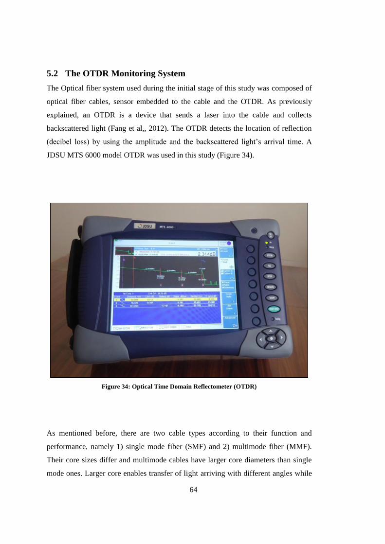
64

5.2 The OTDR Monitoring System

The Optical fiber system used during the initial stage of this study was composed of

optical fiber cables, sensor embedded to the cable and the OTDR. As previously

explained, an OTDR is a device that sends a laser into the cable and collects

backscattered light (Fang et al,, 2012). The OTDR detects the location of reflection

(decibel loss) by using the amplitude and the backscattered light’s arrival time. A

JDSU MTS 6000 model OTDR was used in this study (Figure 34).

Figure 34: Optical Time Domain Reflectometer (OTDR)

As mentioned before, there are two cable types according to their function and

performance, namely 1) single mode fiber (SMF) and 2) multimode fiber (MMF).

Their core sizes differ and multimode cables have larger core diameters than single

mode ones. Larger core enables transfer of light arriving with different angles while

65

single mode cables could only transfer light coming with a right angle. To compose

the optical fiber system using OTDR, these two cable types were used together to

form sensors. The sensors are the sensitive regions generated by splicing cables

having different sizes and characteristics. Several combinations were tested and the

optimum arrangement was found as placing a single mode fiber between two

multimode fiber cables (Kelam et al., 2013). Figure 35 explains the structure of the

sensor.

Figure 35: Basic structure of the heterecore

The logic behind the sensors is the mode difference in fiber cables where multimode

cables have larger modes and higher core diameters than single mode fibers

(Watanabe et al., 2000). Multimode cables can accommodate light coming with

different angles as a result of their larger mode diameter while single mode cables

transfer light with a right angle. Due to this diameter change, the light launched from

the source (i.e., OTDR) travels through the multimode cable and some of the light is

lost when it arrives to a sensor point as the fiber mode changes. This loss enables

sensitive regions to be formed.

66

Figure 36: The utilized fusion splicer (Fujikura FSM 60S) to fuse two cables without signal loss

During the fusion process, a Fujikura FSM 60S model fusion splicer (Figure 36) was

used to splice the cables and also the Fujikura CT-30 model high precision cleaver

(Figure 37) was used to cut the cables at a right angle in order to minimize extra

losses which may originate from the sensor itself.

67

Figure 37: Cleaver used to cut the fiber cables properly

During this study, several cable pairs were spliced and their sensitivities were

analyzed in order to decide the most suitable cable pair. The OTDR shows changes

in cable as decibel losses. Table 9 gives the decibel loss values of different cable

pairs for certain displacements. In addition, graphs of given displacement values can

be seen as Figure 38, Figure 39 and Figure 40.

68

Table 9: Losses of different cable pairs based on displacement

Displacement Loss of Loss of Loss of

62.5-G652D-62.5 62.5-DSF-62.5 62.5-NZDSF-62.5

Initial 3,329 3,143 4,011

1cm 3,866 3,980 4,827

2cm 4,612 4,238 5,408

3cm 5,522 4,620 5,780

4cm 6,390 5,175 5,544

5cm 7,127 5,315 6,084

6cm 7,330 5,434 6,351

7cm 7,623 5,336 6,481

8cm 8,367 5,400 6,487

9cm 7,789 5,377 6,516

Figure 38: Energy loss and displacement relation for the cable pair of 62.5 and G652D

y = -68.99x2 + 1224.9x + 2574.3

R² = 0.9831

0

1.000

2.000

3.000

4.000

5.000

6.000

7.000

8.000

9.000

0 2 4 6 8 10

En

erg

y L

oss

(d

B)

Displacement (cm)

Energy Loss With Changing Displacement

62.5-G652D-62.5

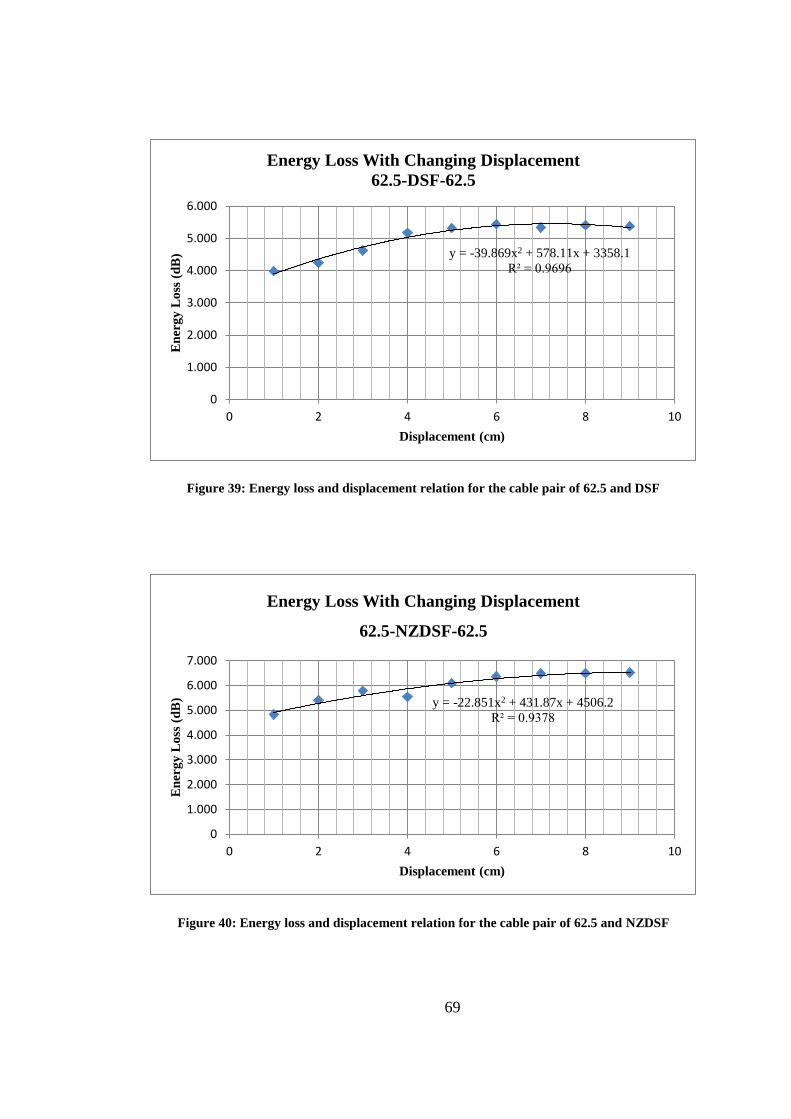
69

Figure 39: Energy loss and displacement relation for the cable pair of 62.5 and DSF

Figure 40: Energy loss and displacement relation for the cable pair of 62.5 and NZDSF

y = -39.869x2 + 578.11x + 3358.1

R² = 0.9696

0

1.000

2.000

3.000

4.000

5.000

6.000

0 2 4 6 8 10

En

erg

y L

oss

(d

B)

Displacement (cm)


62.5-DSF-62.5

y = -22.851x2 + 431.87x + 4506.2

R² = 0.9378

0

1.000

2.000

3.000

4.000

5.000

6.000

7.000

0 2 4 6 8 10

En

erg

y L

oss

(d

B)

Displacement (cm)


62.5-NZDSF-62.5

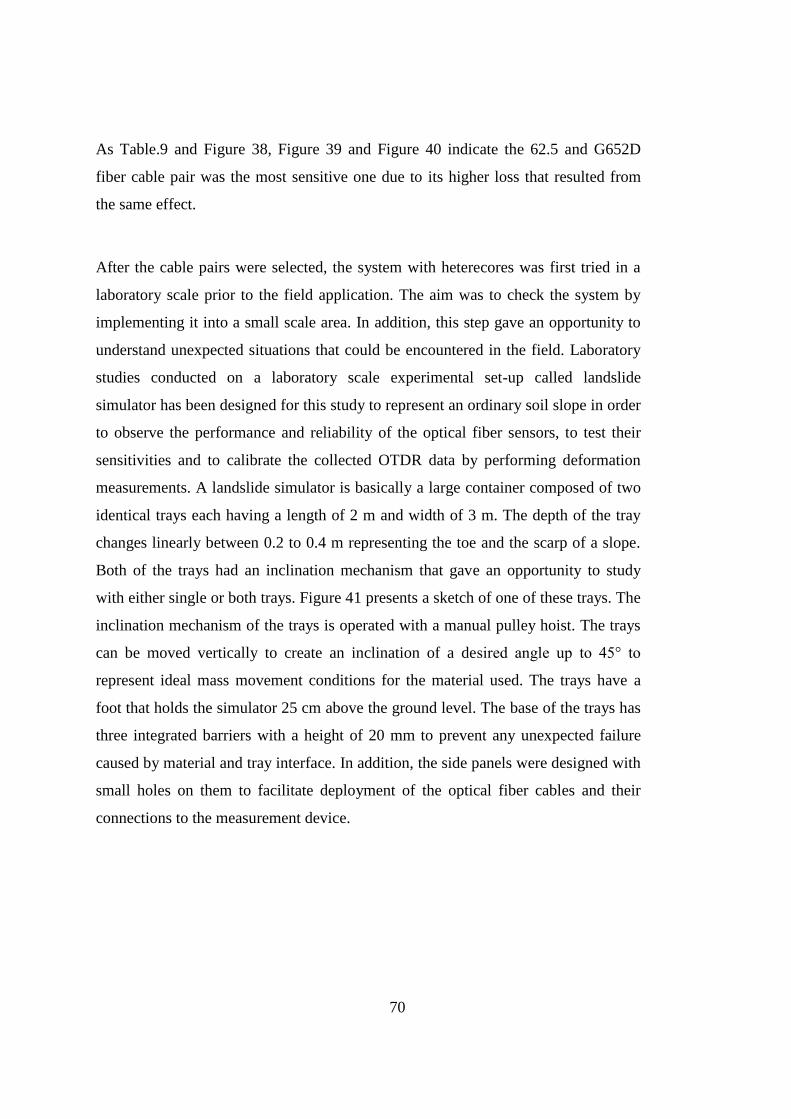
70

As Table.9 and Figure 38, Figure 39 and Figure 40 indicate the 62.5 and G652D

fiber cable pair was the most sensitive one due to its higher loss that resulted from

the same effect.

After the cable pairs were selected, the system with heterecores was first tried in a

laboratory scale prior to the field application. The aim was to check the system by

implementing it into a small scale area. In addition, this step gave an opportunity to

understand unexpected situations that could be encountered in the field. Laboratory

studies conducted on a laboratory scale experimental set-up called landslide

simulator has been designed for this study to represent an ordinary soil slope in order

to observe the performance and reliability of the optical fiber sensors, to test their

sensitivities and to calibrate the collected OTDR data by performing deformation

measurements. A landslide simulator is basically a large container composed of two

identical trays each having a length of 2 m and width of 3 m. The depth of the tray

changes linearly between 0.2 to 0.4 m representing the toe and the scarp of a slope.

Both of the trays had an inclination mechanism that gave an opportunity to study

with either single or both trays. Figure 41 presents a sketch of one of these trays. The

inclination mechanism of the trays is operated with a manual pulley hoist. The trays

can be moved vertically to create an inclination of a desired angle up to 45° to

represent ideal mass movement conditions for the material used. The trays have a

foot that holds the simulator 25 cm above the ground level. The base of the trays has

three integrated barriers with a height of 20 mm to prevent any unexpected failure

caused by material and tray interface. In addition, the side panels were designed with

small holes on them to facilitate deployment of the optical fiber cables and their

connections to the measurement device.

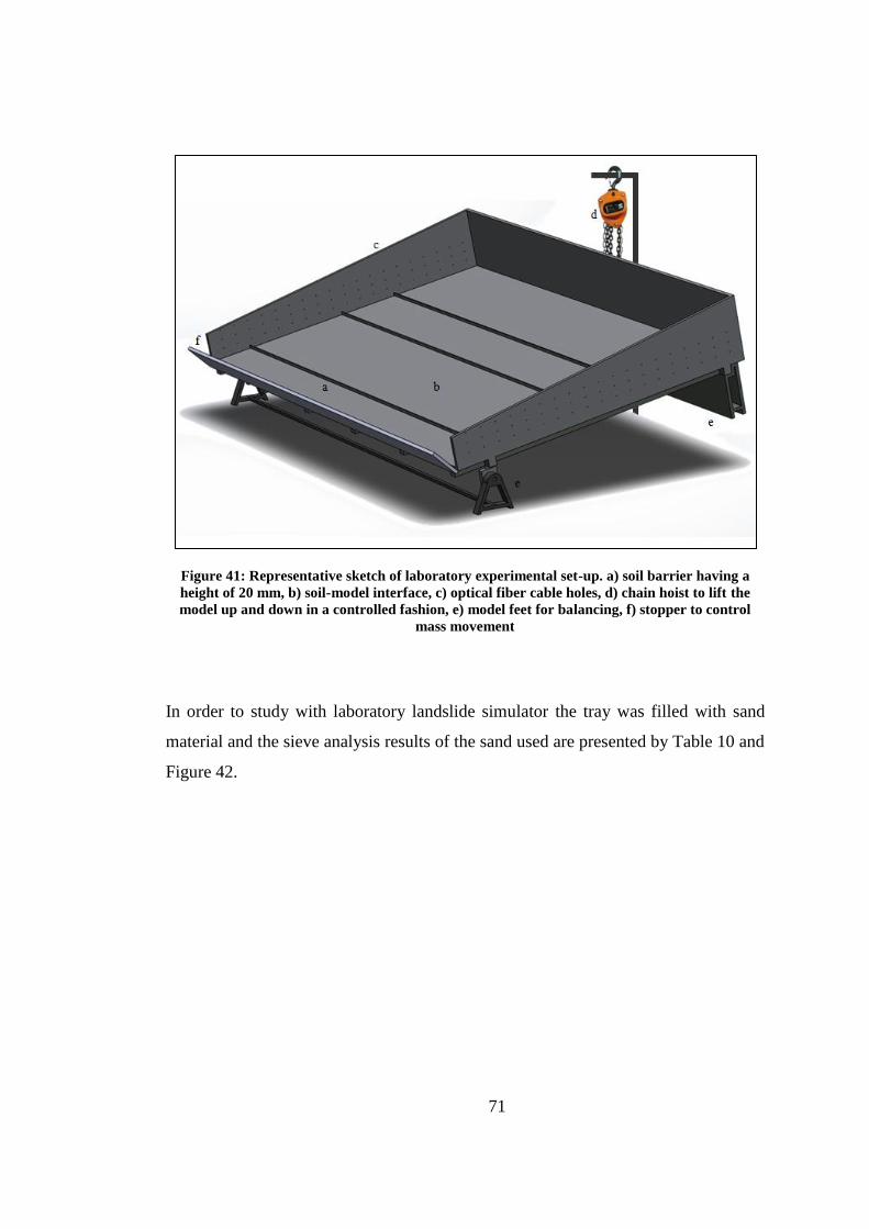
71

Figure 41: Representative sketch of laboratory experimental set-up. a) soil barrier having a

height of 20 mm, b) soil-model interface, c) optical fiber cable holes, d) chain hoist to lift the

model up and down in a controlled fashion, e) model feet for balancing, f) stopper to control

mass movement

In order to study with laboratory landslide simulator the tray was filled with sand

material and the sieve analysis results of the sand used are presented by Table 10 and

Figure 42.

72

Table 10: Sieve analysis data

Test sieve Mass

retained

(g)

Cumulative

mass retained

(g)

Cumulative

% retained

Cumulative

% passing

ASTM

Sieves

Sieve Size

(mm)

No.4 4.750 23 23 4.637096774 95.36290323

No.10 2.000 175 198 39.91935484 60.08064516

No.20 0.850 138 336 67.74193548 32.25806452

No.40 0.425 73 409 82.45967742 17.54032258

No.60 0.250 46 455 91.73387097 8.266129032

No.140 0.106 34 489 98.58870968 1.411290323

No.200 0.075 4 493 99.39516129 0.60483871

Pan 3 496 100 0

Figure 42: Sieve analysis result for the sand used

0

10

20

30

40

50

60

70

80

90

100

0,010 0,100 1,000 10,000

Per

cen

t F

iner

Th

an

(%

)

Particle Size (mm)

Sieve Analysis Graph of Sand

73

From the sieve analysis, D60, D30, and D10 values were calculated as 1.871, 0.750,

and 0.269, respectively. By using these data, the coefficient of uniformity and the

coefficient of curvature were calculated by using Equation 9 and Equation 10.

(9)

(10)

As a consequence, the sand is classified according to unified soil classification

system (USCS) as well graded sand, gravelly sands with little or no fines (SW). The

USCS table is given in Appendix D.

Figure 43 and Figure 44 show the landslide simulator before and after movement

based on inclination, respectively.

74

Figure 43: OTDR sytem measurement in landslide simulator before a movement based on

inclination

Figure 44: OTDR sytem measurement in landslide simulator after a small movement based on

incination

75

Laboratory tests showed that the OTDR system is a sensitive and useful system for

laboratory scale measurements. After the laboratory experiments were completed the

aim was to implement the system to a landslide area. However, this aim could not be

accomplished with the OTDR and this fiber optic setup due to the fragile structure of

heterecores and the limited number of usable heterocores as a result of high energy

loss. The laboratory test with the OTDR, on the other hand, allows finding a relation

between the energy loss and displacement (Equation 11).

(11)

Since the system constructed with the OTDR efficiently responses to the

displacements occurred in a short distance that can be scanned by using three

heterocore sensors, it is obvious that application of this monitoring system in large

scale landslides is not that suitable because as shown in the table, even a single

heterocore sensor reacts to a 1 cm displacement with a 3dB loss which indicates a

power loss around 50%. It means that after the system senses a 3rd

displacement, the

maximum remaining power is around 10% of the initial one. That is why the device

has had problems in taking measurements after the 3rd

point and sensed the fourth

point as the cable end (Arslan et al., 2014). This problem could be resolved by

combining optical amplifiers to the sensors but that wouldn’t be a cost effective

solution.

Because of this problem it was realized that to monitor a large scale area, the system

utilized should be loss-independent which means that it should use a different

parameter than the intensity of the light. All these facts directed the project to

construct a new system by using BOTDA which enables to detect absolute and

76

relative strains along an entire cable free of power loss by observing frequency shifts

which will be given in detail in the following titles.

5.3 The BOTDA Monitoring System

It is possible to reach displacement results by using the OTDR by the correlation of

the decibel losses recorded in a laboratory environment by the aid of a sensitivity

analysis (Kelam et al., 2013). Unfortunately, the dB loss logic behind the OTDR

makes its usage difficult in field applications as the power of light decreases with

every loss. These disadvantages make calibration of the OTDR results complicated

and less accurate. To overcome such negative effects and to increase efficiency and

accuracy, Brillouin-OTDR (BOTDA) systems that detect strain and temperature

changes have started to be used as an alternative (Wu et al., 2002).

The BOTDA requires two laser beams having opposite directions in a fiber cable

layout. One of them is light launched to the cable and the other is backscattered light.

A peak point manifests itself on the resulting measurement graph when the

frequency difference between these two lasers coincides to the Brillouin frequency

of a fiber (Xiaofei et al., 2011).

The strain and temperature changes cause the peak point to form in a different

position than that of its former position. This change is observed as a frequency shift

of the peak point. The BOTDA system is capable of acquiring measurements along a

long fiber layout with a high accuracy. Due to this advantage, in addition to strain

measurement, BOTDA can be used for monitoring of deformation in engineering

structures (Xiaofei et al., 2011; Yin et al., 2010).

Studies were conducted with a Distributed Strain and Temperature Sensor (DSTS)

device manufactured by OZ Optics, Ltd. Similar to the OTDR system studies, the

BOTDA experiments were initiated in a laboratory environment with sensitivity

measurements. As a result of these initial experiments, the relationship between

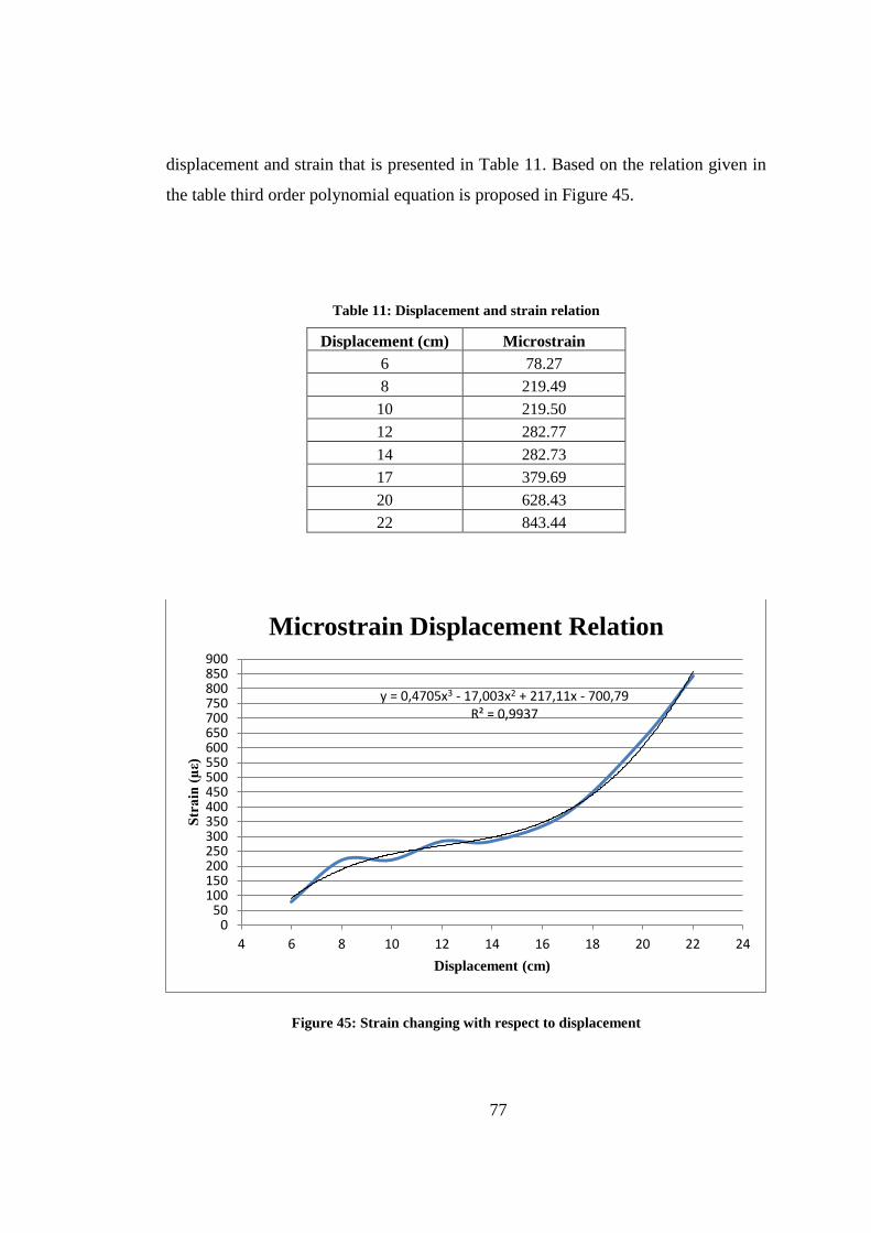
77

displacement and strain that is presented in Table 11. Based on the relation given in

the table third order polynomial equation is proposed in Figure 45.

Table 11: Displacement and strain relation

Displacement (cm) Microstrain

6 78.27

8 219.49

10 219.50

12 282.77

14 282.73

17 379.69

20 628.43

22 843.44

Figure 45: Strain changing with respect to displacement

y = 0,4705x3 - 17,003x2 + 217,11x - 700,79 R² = 0,9937

050

100150200250300350400450500550600650700750800850900

4 6 8 10 12 14 16 18 20 22 24

Str

ain

(µ

ε)

Displacement (cm)

Microstrain Displacement Relation

78

After acquiring this calibration relationship, studies on the landslide simulator were

initiated. Figure 46 and Figure 47 show before and after condition of the experiment,

respectively.

Figure 46: Initial state of the BOTDA system on the laboratory simulator before sliding

Figure 47: Appearance of the BOTDA system after given inclination after sliding

79

As can be observed from the figures, mass movement occurred and the resultant

strain was recorded by the BOTDA. Figure 48 shows the results acquired at the end

of the experiment where the graph gives the strain resulting from slopes with varying

inclination. Blue line represents initial strain present on fiber cable and red, green

and yellow lines represents the strain conditions when the landslide simulator

inclined to 10°, 20° and 30°.

Figure 48: Microstrains formed due to changing inclination of the landslide simulator (red line

represents the measurement taken at 10° inclination, green represents 20° and yellow represents

30° inclination).

5.4 Field Application of the Monitoring System

Field application of the system was implemented at the landslide region that is

located in the Bahçecik Settlement Area of Başiskele District, Kocaeli Province,

Cable ends

Area of interest where

sliding occured

Length of the optical fiber

Movement

direction

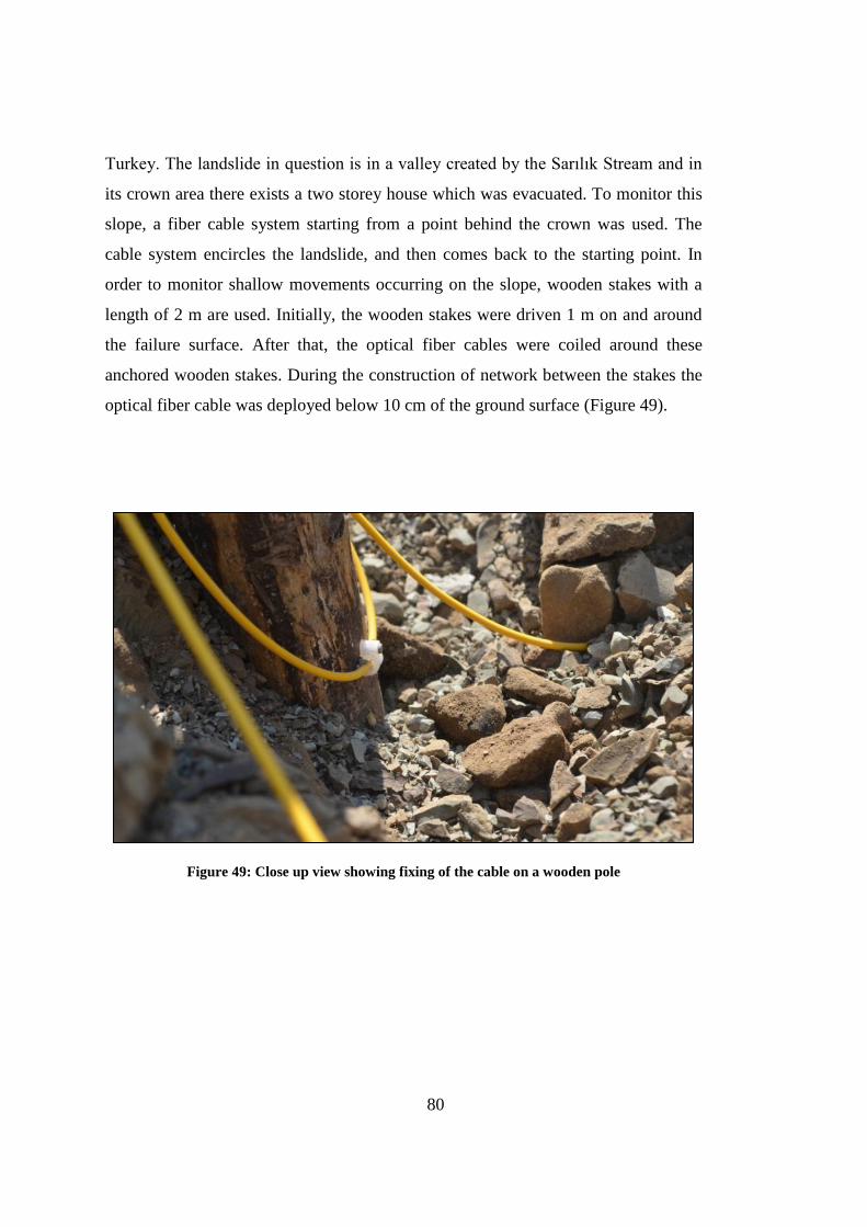
80

Turkey. The landslide in question is in a valley created by the Sarılık Stream and in

its crown area there exists a two storey house which was evacuated. To monitor this

slope, a fiber cable system starting from a point behind the crown was used. The

cable system encircles the landslide, and then comes back to the starting point. In

order to monitor shallow movements occurring on the slope, wooden stakes with a

length of 2 m are used. Initially, the wooden stakes were driven 1 m on and around

the failure surface. After that, the optical fiber cables were coiled around these

anchored wooden stakes. During the construction of network between the stakes the

optical fiber cable was deployed below 10 cm of the ground surface (Figure 49).

Figure 49: Close up view showing fixing of the cable on a wooden pole

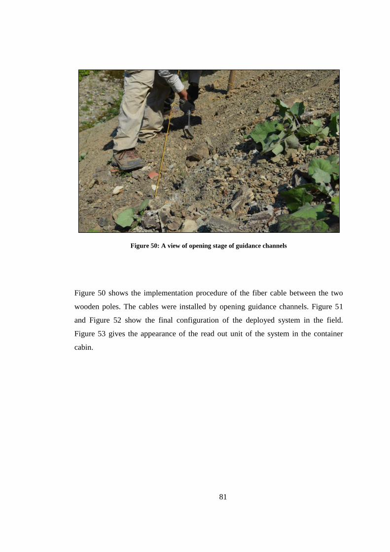
81

Figure 50: A view of opening stage of guidance channels

Figure 50 shows the implementation procedure of the fiber cable between the two

wooden poles. The cables were installed by opening guidance channels. Figure 51

and Figure 52 show the final configuration of the deployed system in the field.

Figure 53 gives the appearance of the read out unit of the system in the container

cabin.

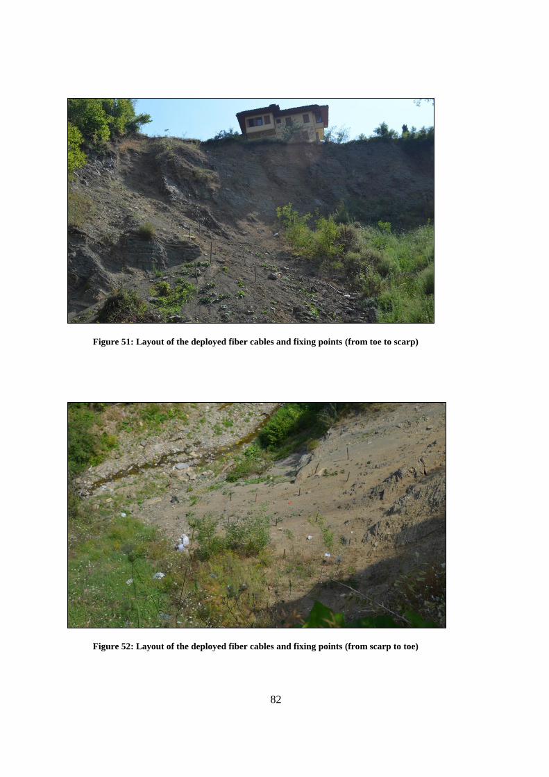
82

Figure 51: Layout of the deployed fiber cables and fixing points (from toe to scarp)

Figure 52: Layout of the deployed fiber cables and fixing points (from scarp to toe)

83

A total of 15 stakes were used and the cable fixed to these poles covers the cable

length between 2005 and 2056 meters. The stakes were tried to be deployed as

equally spaced as possible. These stake locations were decided based on the

deformation analysis explained and given in slope stability chapter (Chapter 3.5) in

order to find the most critical region where the largest mass movement can occur

(Figure 54).

Figure 53: The monitoring unit of the field set up in the container

84

Figure 54: Landslide geometry shown together with deformation contours and cable fixing

points

After the system was deployed, a base measurement was taken and the system was

initialized to monitor the slope. Figure 55 gives the measurement of the entire cable

length while Figure 56 shows the region where the cable was deployed into the

landslide. In Figure 55 and Figure 56 letters A and B are the markers representing

the borders of the deployed length. The optical fiber cable used for field application

can be seen in Appendix E.

85

Figure 55: Baseline measurement of the whole cable

Figure 56: A close up view of the related portion of the cable along with the representative daily

measurements taken during three days

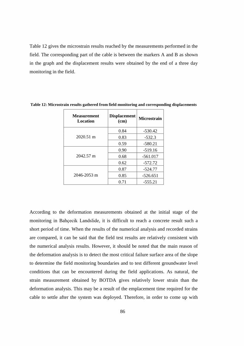
86

Table 12 gives the microstrain results reached by the measurements performed in the

field. The corresponding part of the cable is between the markers A and B as shown

in the graph and the displacement results were obtained by the end of a three day

monitoring in the field.

Table 12: Microstrain results gathered from field monitoring and corresponding displacements

Measurement

Location

Displacement

(cm) Microstrain

2020.51 m

0.84 -530.42

0.83 -532.3

0.59 -580.21

2042.57 m

0.90 -519.16

0.68 -561.017

0.62 -572.72

2046-2053 m

0.87 -524.77

0.85 -526.651

0.71 -555.21

According to the deformation measurements obtained at the initial stage of the

monitoring in Bahçecik Landslide, it is difficult to reach a concrete result such a

short period of time. When the results of the numerical analysis and recorded strains

are compared, it can be said that the field test results are relatively consistent with

the numerical analysis results. However, it should be noted that the main reason of

the deformation analysis is to detect the most critical failure surface area of the slope

to determine the field monitoring boundaries and to test different groundwater level

conditions that can be encountered during the field applications. As natural, the

strain measurement obtained by BOTDA gives relatively lower strain than the

deformation analysis. This may be a result of the emplacement time required for the

cable to settle after the system was deployed. Therefore, in order to come up with

87

firm results, sensitivity analysis should be continued in the field and the monitoring

should be implemented for a longer period such as 3 or 5 months.

89

CHAPTER 6

6. DISCUSSION AND CONCLUSIONS

The main aim of the thesis study is to construct an early warning system by using

optical fiber technology. Optical fiber systems were preferred because of their

advantages over other methods like small size, wide bandwidth, immunity to

electromagnetic interference, resistance to environmental conditions, easy data

transfer, low cost, and real time monitoring. Although, the adopted technology has

not been used as an early warning system yet, the conducted laboratory and field

experiments show that it is capable of determining any type of mass movement.

At the initial stages of the study which had started with the Techno-Initiative Capital

Support Program of Ministry of Science, Industry and Technology and continued

with Research and Development, Innovation and Industrial Application Support

Program of Republic of Turkey Small and Medium Enterprises Development

Organization supports, an optical fiber system using the OTDR as a measurement

device was used with bare fibers. The experiment with the OTDR system led to

determine the sensor generation stage, test stage of its usefulness in the laboratory

and the field implementation stage. The sensors were generated and the system was

tested in laboratory scale by using a landslide simulation model having an inclination

mechanism designed to represent a slope.

The system utilized with the OTDR was very sensitive as a point sensor and it was

capable of measuring the strain in terms of centimeters. Although the system was

sufficient for laboratory studies, it was not applicable to the field as power loss based

90

measurement caused only three sensors to be used. In order to overcome the

limitations of the OTDR, a new system based on the Brillouin frequency shift was

used by the support of the National Earthquake Research Program (UDAP) of

Republic of Turkey, Prime Ministry Disaster and Emergency Management Authority

(AFAD). By the BOTDA system, the same procedure was followed. First, the

system was tested in the laboratory simulator and then applied to field study.

Laboratory studies performed led to a conclusion that the system was suitable for a

landslide monitoring study and measurements resulted with a nonlinear relation

between the strain and displacement. Following the laboratory scale studies, the

system was applied to a landslide region in the Kocaeli Province, Başiskele District,

Bahçecik Settlement Area. This area was selected, because of its critical situation in

terms of landslide risk. In 2010, a landslide occurred and the region was announced

as a hazard prone area by the Republic of Turkey Prime Ministry Disaster and

Emergency Management Authority (AFAD) as the landslide was threatening a house

that was located in the crown area. The BOTDA monitoring system was

implemented to the landslide by deploying optical fiber cables with the help of fixing

points and measurements were collected for few days.

The study area is located in a valley that lies within the stream bed of the Sarılık

stream that is situated in a shear zone and the field observations showed that the

units present in the area is the Paleocene-Eocene aged İncebel formation composed

of sandstone-siltstone-marl alternation. The engineering geological assessment of the

region was made by a field discontinuity scan-line survey and engineering geological

boring logs. According to obtained field data, the formation is classified as very poor

rock mass having soil-like lithology characteristics and it was highly weathered. The

GSI rock mass classification system was used to reach the rock mass parameters

required for the deformation analysis.

In order to understand the triggering mechanism of the landslide, initially, the

seismic activity around the study area was examined and it was concluded that there

has not been any important seismic activity that was capable of triggering the

91

landslide. After this information, the Turkish State Meteorological Service database

revealed that in December, 2010 there was a drastic increase in the rainfall

precipitation values at Kocaeli. The average precipitation was 124.5 mm for

December, 2010 while the average of the December precipitation was 108 mm. In

addition, the precipitation reached a peak value with a daily precipitation of 28.4 mm

on December 10, 2010 which might have been the triggering mechanism of the

landslide.

The displacements take place in a small scale laboratory landslide simulator is rather

obvious; however this is not the case for field application. Therefore, slope stability

analyses were conducted.For this particular objective, a back analysis was

implemented to reach the mobilized shear strength parameters of the moved mass by

using three profiles. The back analysis was implemented by considering saturated

condition at the time of failure and the surcharge of the houses that are located at the

crown of the landslide. Then, the landslide was modeled based on deformation

analysis via the finite element method to compute the displacements. The main

purpose of applying finite element solution was to understand deformation

characteristics of the field and to locate the place where the most deformation might

occur. Accordinly, the monitoring system was deployed to the region to monitor the

slope movement determined by deformation analysis. Another aim of the finite

element solution was to evaluate the effect of grounwater level that can possibly be

changed the stability results during the field monitoring study.

These results showed that the displacement values calculated were in fairly well

agreement with those obtained through field monitoring within a small period of

time. Although the field measurements performed was the preliminary study and the

area should be monitored for a longer time period to reach the conclusive

deformation results, the limited data measured in the study area was quite

reasonable. The optical fiber monitoring system detected a displacement interval of

92

0.59-0.90 cm and the deformation analysis gave displacement values between 0.72-

0.99 cm.

93

CHAPTER 7

7. RECOMMENDATIONS

This thesis study demonstrated that the optical fiber system is a reasonable tool as a

landslide monitoring. At the end of the thesis, the monitoring result that is suitably

compare with the deformation analysis was obtained. Also, calculated deformation

results will be useful to understand anticipated excessive precipitation conditions in

the future for the monitoring study. As mentioned previously, this study will

continue to characterize slope movement through monitoring for a prolonged period

of time as needed.

During the study period, preliminary results were gathered from the monitoring.

Besides, deformation analysis conducted to locate the most critical failure surface in

the study area. Results obtained from the both analysis present similar results but

may not be representative as cables require an emplacement time to settle after the

system was deployed. Therefore, in order to come up with firm results, sensitivity

analysis should be continued in the field and the monitoring results should be

implemented for a longer period of time. In addition, groundwater level on the

region should be monitored as the landslided has triggered by precipitation of

rainfall. For this purpose, a few piozometers might be deployed in the study area to

control the results. In this period, deformation analysis will be detailed and

monitoring system will be converted to an early warning system by asigning treshold

displacement values to the system and controlling it with a GPRS system for

remotely access monitoring or any other system that can replace it.

95

REFERENCES

Abramson, L., W., Lee, T., S., Sharma, S. & Boyce, G., M. (2002), Slope Stability

and Stabilization Methods, John Wiley & Sons, Inc., New York, p. 712.

Akgün, A. & Bulut, F. (2007). GIS-Based Landslide Susceptibility For Arsin-Yomra

(Trabzon, North Turkey) Region. Environmental Geology 51, pp. 1377-1387.

Al-Azzawi, A. (2007). Fiber Optics Principles and Practices. Taylor & Francis

Group: Boca Raton.

Altuğ, G. (2007). Fiber Optik Grating Sensörler. Yüksek Lisans Tezi, Gazi

Üniversitesi.

Ambraseys, N.N. & Zatopek, A. (1969). The Mudurnu Valley, West Anatolia,

Turkey, Earthquake of 22 July 1967. Bull. Seismol. Soc. America, 59, 521-

589.

Arslan, A., Kelam, M. A., Eker, A. M., Akgün, H. & Koçkar, M. K., (2014). Optical

Fiber Technology To Monitor Slope Movement. Engineering Geology For

Society And Territory Volume 2: Landslide Processes. Springer (eBook).

Barnoski, J. K. & Jensen, S. M. (1976). Fiber Waveguides: A Novel Technique For

İnvestigating Attenuation Characteristics. Applied Optics,vol. 15, no.9,

optical society of America.

Barka, A. (1996). Slip Distribution Along The North Anatolian Fault Associated

With The Large Earthquakes Of The Period 1939 To 1967. Bull. Seismol.

Soc. America, 86, pp. 1238-1254.

Barka, A., Akyüz, H.S., Altunel, E., Sunal, G. & Çakır, Z., (2002). The Surface

Rupture And Slip Distribution Of The 17 August 1999 Izmit Earthquake (M

7.4), North Anatolian Fault. Bull. Seismol. Soc. America, 92, 43–60.

96

Bromhead, E., N. (1992). The Stability of Slopes, Blacky Academic & Professional,

London, p. 411.

Cambazoğlu, S. (2012). Preparation Of A Source Model For The Eastern Marmara

Region Along The North Anatolian Fault Segments And Probabilistic

Seismic Hazard Assessment Of Düzce Province. Master Thesis, METU,

Ankara, p. 154.

Cruden, D. M. (1991). A Simple Definition of a Landslide. Bulletin of the

International Association of Engineering Geology, 43, pp. 27-29.

Cruden, D. M. & Varnes, D. J. (1996). Landslide Types And Processes (Chapter 3).

In A. K. Turner & R. L. Schuster (Eds.), Landslides: Investigations and

Mitigation. Transportation Research Board Special Report, 247. National

Research Council. Washington, D. C.: National Academy Press.

Duman, T. Y., Emre, O., Doğan, A., Özalp, S. (2005). Step-Over And Bend

Structures Along The 1999 Düzce Earthquake Surface Rupture, North

Anatolian Fault, Turkey. Bull. Seismol. Soc. America, 95, 1250 – 1262.

Duman, T. Y., Nefeslioğlu, H. A., Çan, T., Ateş, Ş., Durmaz, S., Olgun, Ş.,

Hamzaçebi, S. & Keçer, M. (2006). Türkiye Heyelan Envateri Haritası 1/500

000 ölçekli İstanbul paftası. Maden Tetkik Arama Genel Müdürlüğü Özel

yayın serisi-6.

Emre, Ö., Erkal, T., Tchepalyga, A., Kazanci, N., Keçer, M. & Ünay, E. (1998).

Doğu Marmara Bölgesinin Neojen-Kuvaternerdeki Evrimi, Maden Tetkik ve

Arama Dergisi, 120, pp. 233-258.

Emre, Ö., Doğan, A., Duman, T.Y. & Özalp, T. (2011). 1:250.000 Scale Active

Fault Map Series of Turkey. General Directorate of Mineral Research and

Exploration. Ankara-Turkey.

Erendil, M., Göncüoğlu, M. C., Tekeli, O., Aksay, A., Kuşçu, İ., Ürgün, B. M.,

Tunay, G. & Temren, A. (1991). Armutlu Yarımadasının Jeolojisi. MTA

Rapor No. 9165. MTA, Ankara.

97

Fang, Z., Chin, K. K., Qu, R. & Cai, H. (2012). Fundamentals of Optical Fiber

Sensors. John Wiley & Sons, Inc.: New Jersey.

Gedik İ., Pehlivan, Ş., Timur, E., Duru, M., Altun, İ., Akbaş, B., Özcan, İ. & Alan, İ.

(2005). Kocaeli Yarımadasının Jeolojisi. MTA Rapor No. 10774. MTA,

Ankara.

Geolab Geotecnics. (2012). Heyelan ve Şev Duraylılığının Risk Değerlendirme,

İzleme ve Erken Uyarı Sistemi, Sanayi Bakanlığı TGSD Projesi Sonuç

Raporu.

Gökçe, O., Özden, Ş. & Demir, A. (2008). Türkiye’de Afetlerin Mekansal Ve

İstatistiksel Dağılımı Afet Bilgi Envanteri. T.C. Bayındırlık ve İskan

Bakanlığı Afet İşleri Genel Müdürlüğü Afet Etüt ve Hasar Tespit Daire

Başkanlığı. Ankara, p. 117

Göncüoğlu, M.C., Erendil, M., Tekeli, O., Ürgün, B.M., Aksay, A. & Kuşçu, G.

(1986). Armutlu Yarımadası’nın Doğu Kesiminin Jeolojisi. MTA Rapor, No.

7786. MTA, Ankara.

Göncüoğlu, M. C., Erendil, M., Tekeli O., Aksay, A., Kuşçu İ. & Ürgün, B.M.

(1992). Introduction to the Geology Of Armutlu Peninsula. ISGB-92 Guide

Book. Ankara-Turkey.

Görür, N., Şengör, A.M.C., Akkök, R. & Yılmaz, Y. (1983), Pontidlerde Neo-

Tetis'in Kuzey Kolunun Açılmasına Ilişkin Sedimentolojik Veriler. TJK

Bülteni, 26, 11-20.

Grattan, K., T., V. & Meggitt, B., T. (eds.). (2000). Optical Fiber Sensor Technology

Fundamentals. Kluwer Academic Publishers, Dordrecht, Netherlands. pp. 1-

44.

Gupta, S. C. (2012). Textbook On Optical Fiber Communication And İts

Applications (2nd Edition). PHI Learning Private Limited. New Delhi.

Halley, P. (1987). Fibre optic systems. John Wiley & Sons, United Kingdom.

98

HAMA Engineering. (2014). Heyelan Risk Analizi, Takip ve Erken Uyarı Sistemi

(HERATEUS), Kosgeb Ar-Ge İnovasyon Desteği Gelişme Raporu.

Hayes, J. (2006). Fiber Optics Technician’s Manual (third ed.). Thomson Delmar

Learning: Canada.

Hoek E, & Bray JW, (1981). Rock Slope Engineering. London: Institution of

Mining, Metallurgy, p. 358.

Horiguchi, T. , Kurashima, T. & Tateda, M. (1989). Tensile Strain Dependence of

Brillouin Frequency Shift in Silica Optical Fibers. IEEE Photonics

Technology Letters, vol. 1, No. 5, pp. 107-108.

Horiguchi, T., Shimizu, K., Kurashima T., Tateda, M. & Koyamada, Y. (1995).

Development of a Distributed Sensing Technique Using Brillouin Scattering.

Ournal of Lightwave Technology, vol. 13, No. 7.

ISRM. (1981). Suggested Methods For The Quantitative Description Of

Discontinuities In Rock Masses. In: Barton T, editor. Rock Characterization,

Testing And Monitoring. Oxford, London: Pergamon Press, p. 221.

Iten, M. (2011). Novel Applications of Distributed Fiber-Optic Sensing in

Geotechnical Engineering. A Dissertation Submitted To Eth Zurich For The

Degree Of Doctor Of Sciences.

Kandilli Observatory and Earthquake Research Institute (KOERI). (2015).

Earthquake Catalogue, retrieved from Deprem Kataloğu:

http://www.koeri.boun.edu.tr/sismo/2/deprem-verileri/deprem-katalogu/

Kelam, M. A., Eker, A. M., Akgün, H., Arslan, A. & Koçkar, M. K. (2013). A New

Method For Monitoring Landslide And Slope Stability: Optical Fiber

Technology. Proceedings of 66. Turkish Geological Symposium. Ankara, pp

312-313. (Abstract only).

Ketin, I. (1969). Uber die Nordanatolische Horizontalverschiebung. Bull Mineral

Res. Explor. Inst. (MTA) Turkey. 72, 1-28.

99

Kocaeli Environment and Urbanization Directorate. (2011). Kocaeli Environment

Information Report. Retrieved from

http://www.csb.gov.tr/turkce/dosya/ced/icdr2011/kocaeli_icdr2011.pdf

(accessed July 15,2015).

Lettis, W., Bachhuber, J., Witter, R., Brankman, C., Randolph, C.E., Barka, A.,

Page, W.D. & Kaya, A. (2002). Influence Of Releasing Step-Overs On

Surface Fault Rupture And Fault Segmentation: Examples from the 17

August 1999 Izmit earthquake on the North Anatolian Fault, Turkey. Bull.

Seismol. Soc. America, 92(1), 19-42.

Li, F., Du, Y., Zhang, W., Sun, B. & Li, F. (2012). Monitoring System For High

Steep Slope Based On Optical Fiber Sensing Technology. Advanced Sensor

Systems snd Applications V, v. 8561, 85610F.

Liu, Y., Dai, Z., Zhang, X., Peng, Z., Li, J., Ou, Z. & Liu, Y. (2010). Optical Fiber

Sensors For Landslide Monitoring. Semiconductor Lasers and Applications

IV, v. 7844, 78440D.

Mafang, S. F. (2011). Brillouin Echos for Advanced Distributed Sensing in Optical

Fibres, Phd. Thesis, Ecole Polytechnique Federale DE Lausanne.

Marinos, P. & Hoek, E. (2000). GSI: A Geologically Friendly Tool for Rock Mass

Strength Estimation. Proc. International Conference on Geotechnical and

Geological Engineering, GeoEng2000, Technomic publ., pp. 1422-1442

Marinos, V., Marinos, P. & Hoek, E. (2005). The Geological Strength Index:

Applications and Limitations. Bull. Eng. Geol. Env., v. 64, pp. 55-65.

Measures, R., M. (2001). Structural Monitoring With Fiber Optic Technology.

Academic Press, USA.

Mohammed, Z. F. & Fatth, A. Y. (2013). Digital Signal Processing for Cancellation

of Fiber Optic Impairments: Design and Simulation Using OptiSystem and

Matlab. Lambert Academic Publishing: Germany.

http://www.csb.gov.tr/turkce/dosya/ced/icdr2011/kocaeli_icdr2011.pdf

100

MTA. (2003). Atlas of North Anatolian Fault: Special Publications Series:2. MTA

Press, Ankara.

Ohno, H., Naruse, H., Kihara, M. & Shimada, A. (2001). Industrial Applications of

the BOTDR Optical Fiber Strain Sensor. Optical Fiber Technology, 7, pp. 45-

64.

Öztürk, A., İnan, S. & Tutkun, Z. (1985). Abant-Yeniçağa Yöresinin Tektoniği, Bull.

Earth Sci. Cumhuriyet Univ.2, 35-52.

Pei, H., Cui, P., Yin, J., Zhu, H., Chen, X., Pei, L. & Xu D., (2011). Monitoring And

Warning Of Landslides And Debris Flows Using An Optical Fiber Sensor

Technology. J. Mount. Sci., v. 8, pp. 728-738.

Powers, J. (1997). An Introduction to Fiber Optic Systems (second ed.). McGraw-

Hill Professional: USA

Rocscience. (2010). Slide Version 6, Slope Stability and Groundwater Seepage

Analysis, Rocscience Inc. 31 Balsam Ave., Toronto, Ontario M4E 1B2,

Canada.

Rocscience. (2011). Phase2 Version 8, Finite Element Analysis for Excavations and

Slopes, Rocscience Inc. 31 Balsam Ave., Toronto, Ontario M4E 1B2,

Canada.

Rocscience. (2012). DIPS Version 6, Graphical and Statistical Analysis of

Orientation Data, Rocscience Inc. 31 Balsam Ave., Toronto, Ontario M4E

1B2, Canada.

Rocscience. (2014). RocLab Version 1, Rock Mass Strength Analysis Program

Using The Hoek–Brown Failure Criterion, Rocscience Inc. 31 Balsam Ave.,

Toronto, Ontario M4E 1B2, Canada.

Savvaidis, P. D. (2003). Existing Landslide Monitoring Systems And Techniques.

From Stars To Earth And Culture. School of Rural and Surveying

Engineering, The Aristotle University of Thessaloniki, pp. 242-258.

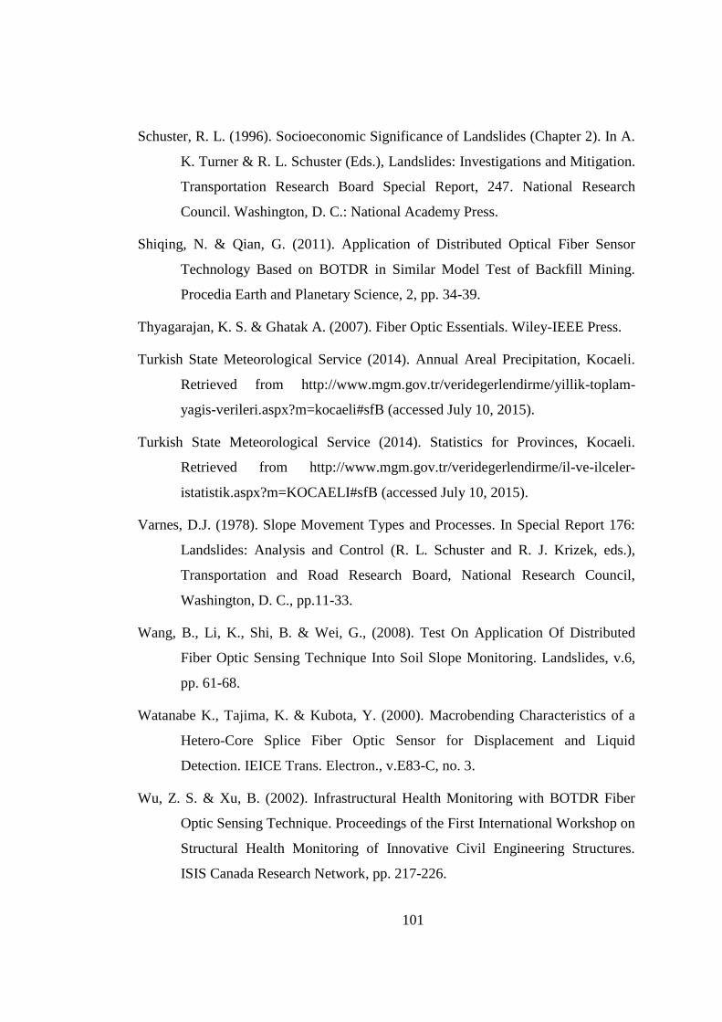
101

Schuster, R. L. (1996). Socioeconomic Significance of Landslides (Chapter 2). In A.

K. Turner & R. L. Schuster (Eds.), Landslides: Investigations and Mitigation.

Transportation Research Board Special Report, 247. National Research

Council. Washington, D. C.: National Academy Press.

Shiqing, N. & Qian, G. (2011). Application of Distributed Optical Fiber Sensor

Technology Based on BOTDR in Similar Model Test of Backfill Mining.

Procedia Earth and Planetary Science, 2, pp. 34-39.

Thyagarajan, K. S. & Ghatak A. (2007). Fiber Optic Essentials. Wiley-IEEE Press.

Turkish State Meteorological Service (2014). Annual Areal Precipitation, Kocaeli.

Retrieved from http://www.mgm.gov.tr/veridegerlendirme/yillik-toplam-

yagis-verileri.aspx?m=kocaeli#sfB (accessed July 10, 2015).

Turkish State Meteorological Service (2014). Statistics for Provinces, Kocaeli.

Retrieved from http://www.mgm.gov.tr/veridegerlendirme/il-ve-ilceler-

istatistik.aspx?m=KOCAELI#sfB (accessed July 10, 2015).

Varnes, D.J. (1978). Slope Movement Types and Processes. In Special Report 176:

Landslides: Analysis and Control (R. L. Schuster and R. J. Krizek, eds.),

Transportation and Road Research Board, National Research Council,

Washington, D. C., pp.11-33.

Wang, B., Li, K., Shi, B. & Wei, G., (2008). Test On Application Of Distributed

Fiber Optic Sensing Technique Into Soil Slope Monitoring. Landslides, v.6,

pp. 61-68.

Watanabe K., Tajima, K. & Kubota, Y. (2000). Macrobending Characteristics of a

Hetero-Core Splice Fiber Optic Sensor for Displacement and Liquid

Detection. IEICE Trans. Electron., v.E83-C, no. 3.

Wu, Z. S. & Xu, B. (2002). Infrastructural Health Monitoring with BOTDR Fiber

Optic Sensing Technique. Proceedings of the First International Workshop on

Structural Health Monitoring of Innovative Civil Engineering Structures.

ISIS Canada Research Network, pp. 217-226.

http://www.mgm.gov.tr/veridegerlendirme/yillik-toplam-yagis-verileri.aspx?m=kocaeli#sfB

http://www.mgm.gov.tr/veridegerlendirme/yillik-toplam-yagis-verileri.aspx?m=kocaeli#sfB

http://www.mgm.gov.tr/veridegerlendirme/il-ve-ilceler-istatistik.aspx?m=KOCAELI#sfB

http://www.mgm.gov.tr/veridegerlendirme/il-ve-ilceler-istatistik.aspx?m=KOCAELI#sfB

102

Xiaofei, Z., Wenjie, H., Qing, Z., Yanxin, S., Xianwei, M. & Yongwen, H., (2011).

Development Of Optical Fiber Strain Monitoring System Based On BOTDR.

The Tenth International Conference on Electronic Measurement &

Instruments (ICEMI), IEEE, v. 4, pp. 38-41.

Yan, E., Song, K. & Li, H. (2010). Applicability Of Time Domain Refelectometry

For Yuhuangge Landslide Monitoring. Journal ofr Earth Sciences, vol. 21,

No.6, pp. 856-860.

Yin, Y., Wang, H., Gao, Y. & Li, X., (2010). Real-Time Monitoring And Early

Warning Of Landslides At Relocated Wushan Town, The Three Gorges

Reservoir, China. Landslides, v. 7, pp. 339-349.

Yücel, M., Göktaş, H. H., Yücel, M. & Öztürk, N.F. (2014). Brillouin Saçılması

Tabanlı Fiber Optik Algılama. IEEE 22. Sinyal İşleme ve İletişim

Uygulamaları Kurultayı Trabzon.

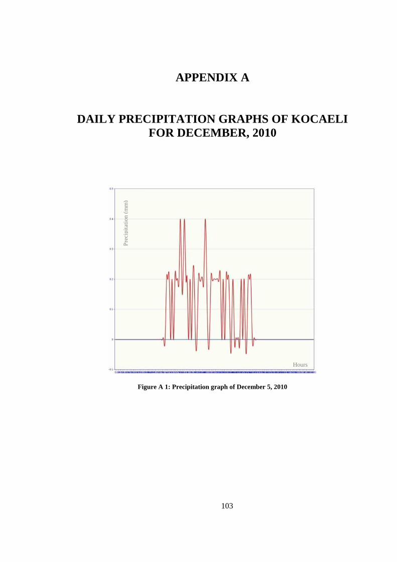
103

APPENDIX A

DAILY PRECIPITATION GRAPHS OF KOCAELI

FOR DECEMBER, 2010

Figure A 1: Precipitation graph of December 5, 2010

Hours

Pre

cipit

atio

n (

mm

)

104



Hours

Hours

Pre

cipit

atio

n (

mm

) P

reci

pit

atio

n (

mm

)

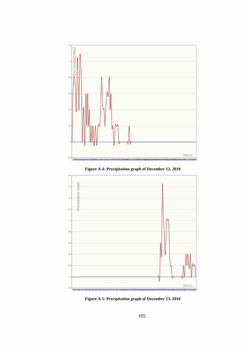
105



Hours

Hours

Pre

cipit

atio

n (

mm

) P

reci

pit

atio

n (

mm

)

106



Hours

Hours

Pre

cipit

atio

n (

mm

) P

reci

pit

atio

n (

mm

)

107



Hours

Hours

Pre

cipit

atio

n (

mm

) P

reci

pit

atio

n (

mm

)

108



Hours

Hours

Pre

cipit

atio

n (

mm

) P

reci

pit

atio

n (

mm

)

109



Hours

Hours

Pre

cipit

atio

n (

mm

) P

reci

pit

atio

n (

mm

)

111

APPENDIX B

BOREHOLE LOGS

Borehole Base

GRAPH

FO

RM

AT

ION

S

AR

ISU

FO

RM

AT

ION

CLAYSTONE-

SANDSTONE

ALTERNATION

SANDY CLAYEY SILT

BLOW COUNT

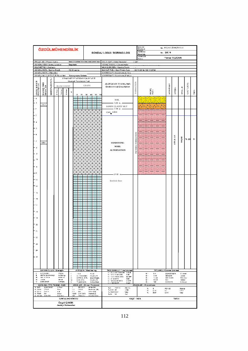
112

SANDSTONE-

MARL

ALTERNATION

Borehole Base

GRAPH

FO

RM

AT

ION

İN

CE

BE

L F

OR

MA

TIO

N

SANDY CLAYEY SILT

SOIL

GWL

BLOW COUNT

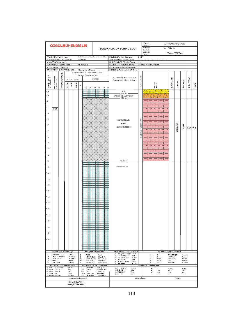
113

SOIL

SANDY CLAYEY SILT

SANDSTONE-

MARL

ALTERNATION

GRAPH

FO

RM

AT

ION

İN

CE

BE

L F

OR

MA

TIO

N

Borehole Base

BLOW COUNT

114

GRAPH

FO

RM

AT

ION

SOIL

SANDY CLAYEY SILT

SANDSTONE-

MARL

ALTERNATION

İNC

EB

EL

FO

RM

AT

ION

Borehole Base

BLOW COUNT

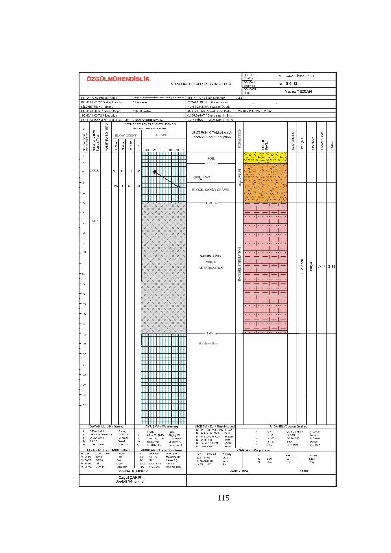
115

GRAPH

FO

RM

AT

ION

SOIL

SANDSTONE-

MARL

ALTERNATION

İNC

EB

EL

FO

RM

AT

ION

Borehole Base

BLOCK, SANDY GRAVEL

GWL

AL

LU

VIU

M

BLOW COUNT

116

BLOCK, SANDY GRAVEL

SOIL

AL

LU

VIU

M

SANDSTONE-

MARL

ALTERNATION

Borehole Base

İNC

EB

EL

FO

RM

AT

ION

GWL

GRAPH

FO

RM

AT

ION

BLOW COUNT

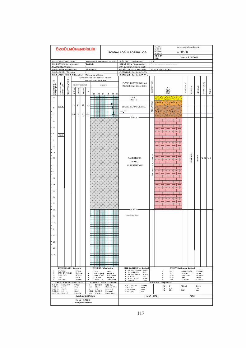
117

GRAPH BLOW COUNT

Borehole Base

İNC

EB

EL

FO

RM

AT

ION

SANDSTONE-

MARL

ALTERNATION

FO

RM

AT

ION

SOIL

BLOCK, SANDY GRAVEL

GWL AL

LU

VIU

M

118

Borehole Base

SANDSTONE-

MARL

ALTERNATION

İNC

EB

EL

FO

RM

AT

ION

BLOW COUNT GRAPH

FO

RM

AT

ION

EMBANKMENT

ROAD EMBANKMENT

119

BLOW COUNT GRAPH

FO

RM

AT

ION

SOIL

SANDSTONE-

MARL

ALTERNATION

Borehole Base

İNC

EB

EL

FO

RM

AT

ION

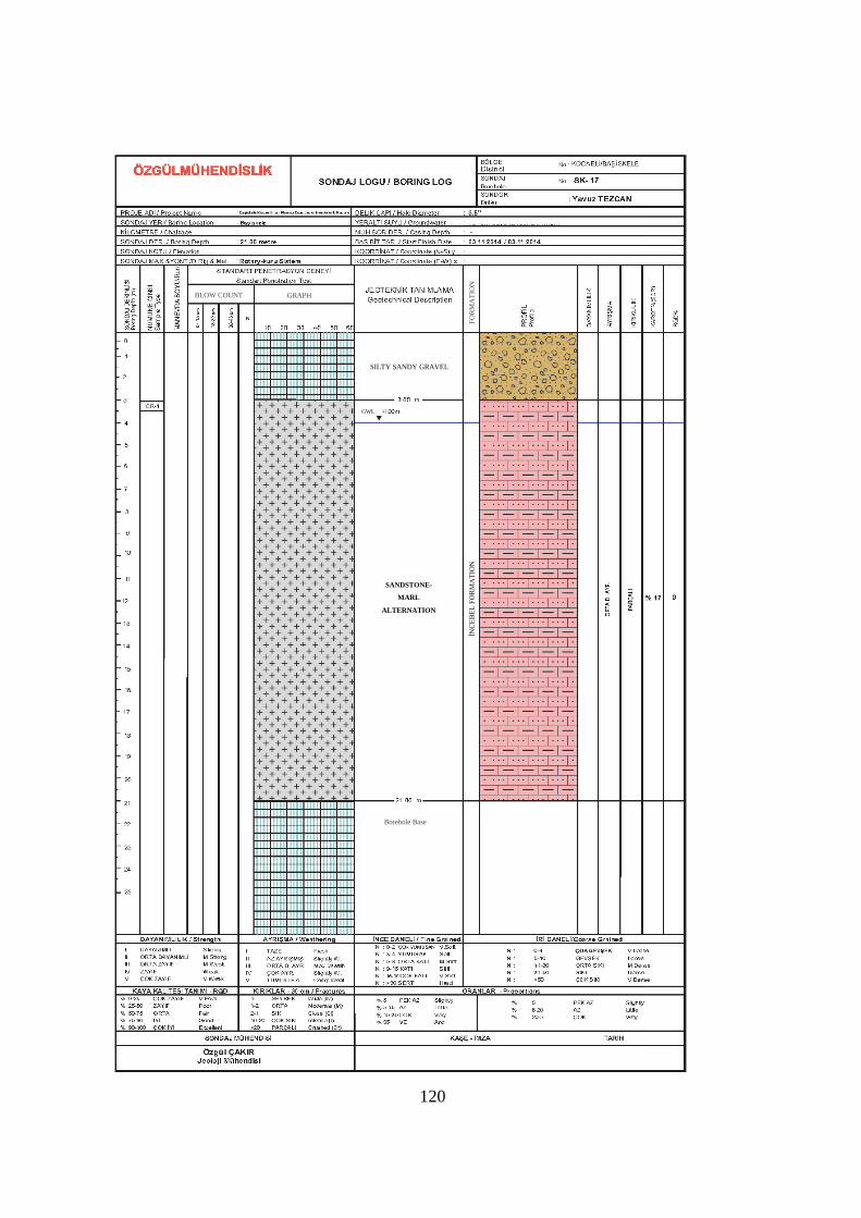
120

Borehole Base

SANDSTONE-

MARL

ALTERNATION

BLOW COUNT GRAPH

FO

RM

AT

ION

SILTY SANDY GRAVEL

İNC

EB

EL

FO

RM

AT

ION

GWL

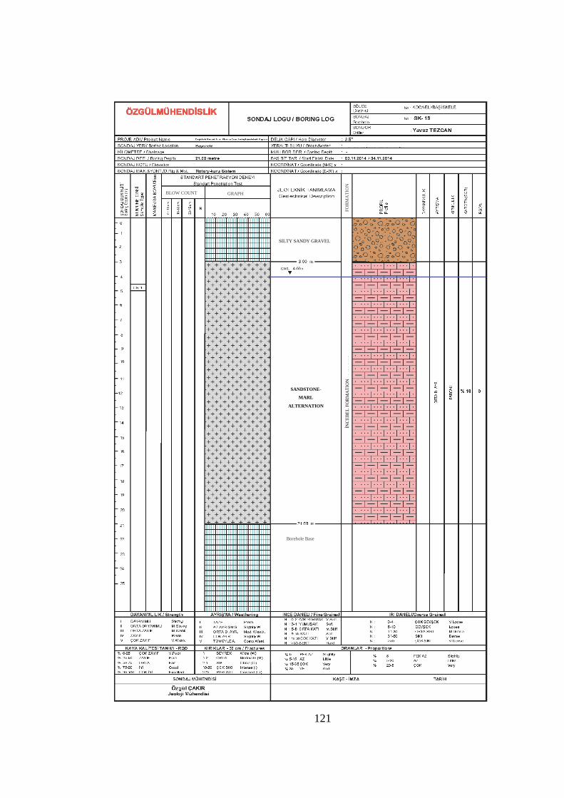
121

Borehole Base

SANDSTONE-

MARL

ALTERNATION

İNC

EB

EL

FO

RM

AT

ION

F

OR

MA

TIO

N

BLOW COUNT GRAPH

SILTY SANDY GRAVEL

GWL

122

Borehole Base

SANDSTONE-

MARL

ALTERNATION

İNC

EB

EL

FO

RM

AT

ION

BLOW COUNT GRAPH

EMBANKMENT

FO

RM

AT

ION

GWL

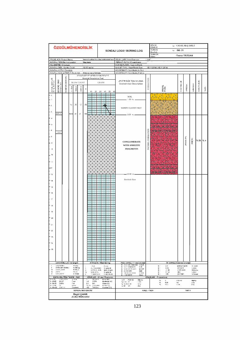
123

BLOW COUNT GRAPH

FO

RM

AT

ION

İN

CE

BE

L F

OR

MA

TIO

N

SOIL

SANDY CLAYEY SILT

Borehole Base

CONGLOMERATE

WITH ANDEZITE

FRAGMENTS

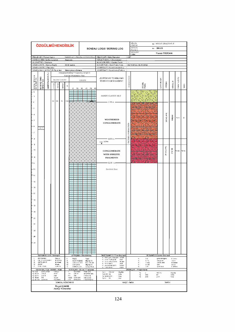
124

CONGLOMERATE

WITH ANDEZITE

FRAGMENTS

İNC

EB

EL

FO

RM

AT

ION

BLOW COUNT GRAPH

FO

RM

AT

ION

Borehole Base

SANDY CLAYEY SILT

WEATHEREED

CONGLOMERATE

GWL

125

APPENDIX C

EARTHQUAKE CATALOGUE OF STUDY AREA

AND ITS SURROUNDINGS FOR 2010

Table C 1: Earthquakes happened in 2010 with a moment magnitude equal and greater than 3.0

Date

Origin

Time Lat. Long

Depth

(km) xM MD ML Type Location

26.01.

2011

16:58:16.

85

39.13

4

28.99

93 5 3 3 0 Ke

HACIAHMETOGLU-SIMAV

(KUTAHYA) [South West 1.3

km]

23.01.

2011

22:01:11.

13

40.47

32

30.16

72 5 3.1 3.1 0 Ke

CARDAK-PAMUKOVA

(SAKARYA) [East 0.8 km]

20.01.

2011

02:09:37.

04

40.70

42

29.76

28 11.7 4.1 0 4.1 Ke

ORCUN-GOLCUK (KOCAELI)

[West 2.7 km]

15.01.

2011

16:00:22.

25

40.79

92

31.36

77 3.3 3.2 3.2 0 Ke

DARIYERIHASANBEY-

KAYNASLI (DUZCE) [North

East 3.4 km]

12.01.

2011

10:31:34.

36

40.14

12

31.73

85 5 3.3 3.3 0 Ke

CANTIRLI-BEYPAZARI

(ANKARA) [West 4.3 km]

16.12.

2010

01:07:55.

53

40.72

58

29.89

75 5.3 3 3 0 Ke KOCAELI [South West 4.1 km]

12.12.

2010

12:20:38.

39

39.80

82 30.5 5 3.1 3.1 0 Ke

TEPEBASI (ESKISEHIR) [North

East 2.7 km]

11.12.

2010

20:16:20.

89

39.12

5

29.06

58 5.4 3 3 0 Ke

SOGUT-SIMAV (KUTAHYA)

[West 1.3 km]

08.12.

2010

20:04:00.

55

39.11

67

29.10

95 5.4 3.2 3.2 0 Ke

SENKOY-SIMAV (KUTAHYA)

[North West 1.9 km]

02.12.

2010

23:01:46.

29

40.08

53

31.65

12 9.3 3 3 0 Ke

CAYIRHAN-NALLIHAN

(ANKARA) [South West 2.7

km]

23.11.

2010

22:16:51.

14

39.12

58

29.04

37 5.4 3 3 0 Ke

KAPIKAYA-SIMAV

(KUTAHYA) [South East 0.8

km]

20.11.

2010

17:23:03.

40

40.10

38

31.67

92 5 3 3 0 Ke

CAYIRHAN-NALLIHAN

(ANKARA) [North 0.8 km]

19.11.

2010

11:33:54.

54

40.95

03

29.22

58 7.8 3 3 3 Ke

SULTANBEYLI (ISTANBUL)

[South West 3.6 km]

12.11.

2010

04:00:30.

18

40.72

58

28.98

93 8.5 3 3 0 Ke

CINARCIK ACIKLARI-

YALOVA (MARMARA

DENIZI)

11.11.

2010

23:03:26.

58

40.09

07

31.59

48 8.7 3 3 0 Ke

DAVUTOGLAN-NALLIHAN


km]

31.10.

2010

03:44:37.

62

40.37

98

30.01

82 3.6 3.1 3.1 0 Ke

SELCIK-OSMANELI

(BILECIK) [East 1.2 km]

26.10.

2010

22:09:40.

55

40.80

23

27.68

08 10.2 3.5 3.2 3.5 Ke MARMARA DENIZI

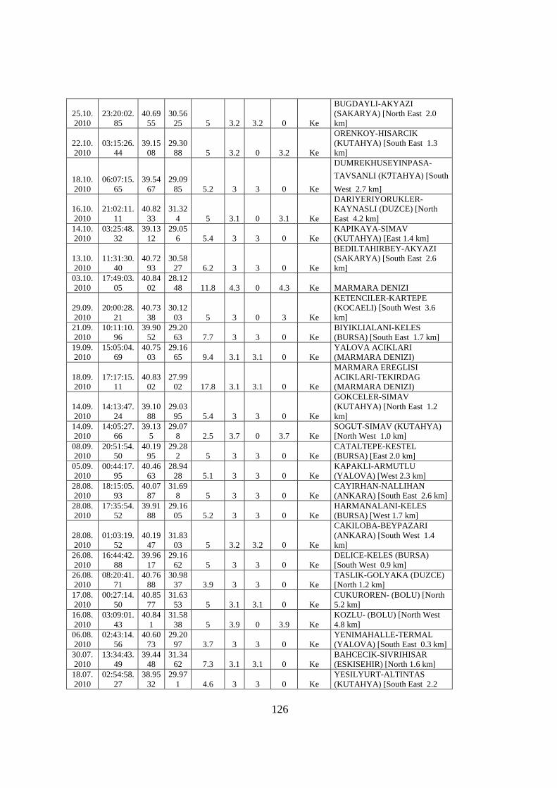
126

25.10.

2010

23:20:02.

85

40.69

55

30.56

25 5 3.2 3.2 0 Ke

BUGDAYLI-AKYAZI

(SAKARYA) [North East 2.0

km]

22.10.

2010

03:15:26.

44

39.15

08

29.30

88 5 3.2 0 3.2 Ke

ORENKOY-HISARCIK


km]

18.10.

2010

06:07:15.

65

39.54

67

29.09

85 5.2 3 3 0 Ke

DUMREKHUSEYINPASA-

TAVSANLI (KﾜTAHYA) [South

West 2.7 km]

16.10.

2010

21:02:11.

11

40.82

33

31.32

4 5 3.1 0 3.1 Ke

DARIYERIYORUKLER-

KAYNASLI (DUZCE) [North

East 4.2 km]

14.10.

2010

03:25:48.

32

39.13

12

29.05

6 5.4 3 3 0 Ke

KAPIKAYA-SIMAV

(KUTAHYA) [East 1.4 km]

13.10.

2010

11:31:30.

40

40.72

93

30.58

27 6.2 3 3 0 Ke

BEDILTAHIRBEY-AKYAZI

(SAKARYA) [South East 2.6

km]

03.10.

2010

17:49:03.

05

40.84

02

28.12

48 11.8 4.3 0 4.3 Ke MARMARA DENIZI

29.09.

2010

20:00:28.

21

40.73

38

30.12

03 5 3 0 3 Ke

KETENCILER-KARTEPE

(KOCAELI) [South West 3.6

km]

21.09.

2010

10:11:10.

96

39.90

52

29.20

63 7.7 3 3 0 Ke

BIYIKLIALANI-KELES

(BURSA) [South East 1.7 km]

19.09.

2010

15:05:04.

69

40.75

03

29.16

65 9.4 3.1 3.1 0 Ke

YALOVA ACIKLARI

(MARMARA DENIZI)

18.09.

2010

17:17:15.

11

40.83

02

27.99

02 17.8 3.1 3.1 0 Ke

MARMARA EREGLISI

ACIKLARI-TEKIRDAG

(MARMARA DENIZI)

14.09.

2010

14:13:47.

24

39.10

88

29.03

95 5.4 3 3 0 Ke

GOKCELER-SIMAV

(KUTAHYA) [North East 1.2

km]

14.09.

2010

14:05:27.

66

39.13

5

29.07

8 2.5 3.7 0 3.7 Ke


[North West 1.0 km]

08.09.

2010

20:51:54.

50

40.19

95

29.28

2 5 3 3 0 Ke

CATALTEPE-KESTEL

(BURSA) [East 2.0 km]

05.09.

2010

00:44:17.

95

40.46

63

28.94

28 5.1 3 3 0 Ke

KAPAKLI-ARMUTLU

(YALOVA) [West 2.3 km]

28.08.

2010

18:15:05.

93

40.07

87

31.69

8 5 3 3 0 Ke

CAYIRHAN-NALLIHAN

(ANKARA) [South East 2.6 km]

28.08.

2010

17:35:54.

52

39.91

88

29.16

05 5.2 3 3 0 Ke

HARMANALANI-KELES

(BURSA) [West 1.7 km]

28.08.

2010

01:03:19.

52

40.19

47

31.83

03 5 3.2 3.2 0 Ke

CAKILOBA-BEYPAZARI


km]

26.08.

2010

16:44:42.

88

39.96

17

29.16

62 5 3 3 0 Ke

DELICE-KELES (BURSA)

[South West 0.9 km]

26.08.

2010

08:20:41.

71

40.76

88

30.98

37 3.9 3 3 0 Ke

TASLIK-GOLYAKA (DUZCE)

[North 1.2 km]

17.08.

2010

00:27:14.

50

40.85

77

31.63

53 5 3.1 3.1 0 Ke

CUKUROREN- (BOLU) [North

5.2 km]

16.08.

2010

03:09:01.

43

40.84

1

31.58

38 5 3.9 0 3.9 Ke

KOZLU- (BOLU) [North West

4.8 km]

06.08.

2010

02:43:14.

56

40.60

73

29.20

97 3.7 3 3 0 Ke

YENIMAHALLE-TERMAL

(YALOVA) [South East 0.3 km]

30.07.

2010

13:34:43.

49

39.44

48

31.34

62 7.3 3.1 3.1 0 Ke

BAHCECIK-SIVRIHISAR

(ESKISEHIR) [North 1.6 km]

18.07.

2010

02:54:58.

27

38.95

32

29.97

1 4.6 3 3 0 Ke

YESILYURT-ALTINTAS


127

km]

17.07.

2010

19:39:50.

44

40.71

15

29.19

97 5 3.1 3.1 0 Ke

YALOVA ACIKLARI

(MARMARA DENIZI)

09.07.

2010

12:09:45.

85

38.96

62

29.96

95 2 3 3 0 Ke

YESILYURT-ALTINTAS


km]

07.07.

2010

10:24:49.

31

40.80

88

30.88

17 9.2 3.3 0 3.3 Ke

YESILYAYLA-GUMUSOVA

(DUZCE) [North East 1.6 km]

07.07.

2010

04:02:07.

35

39.16

03

29.03

48 5.2 3 3 0 Ke

KARACAOREN-SIMAV


km]

06.07.

2010

16:01:33.

27

40.42

5

28.42

8 2.3 3 3 0 Ke

BAYRAMDERE-KARACABEY

(BURSA) [North East 5.6 km]

13.06.

2010

02:13:25.

17

39.19

42

29.12

12 5 3.1 3.1 0 Ke

TOKAT-HISARCIK


km]

11.06.

2010

23:45:42.

16

39.11

55

29.13

72 5 3 3 0 Ke


[North East 2.0 km]

09.06.

2010

16:06:56.

05

39.29

2

29.08

38 5.4 3.3 0 3.3 Ke

KABAKLAR-EMET

(KUTAHYA) [North West 2.5

km]

02.06.

2010

19:09:32.

85

39.49

92

28.85

88 6.9 3 0 3 Ke

MAHMUTCA-DURSUNBEY

(BALIKESIR) [South West 0.2

km]

31.05.

2010

16:08:20.

25

39.02

32

29.73

52 5.3 3 3 0 Ke

CUKUROREN-GEDIZ

(KUTAHYA) [North 3.1 km]

29.05.

2010

22:36:04.

04

40.94

6

31.73

38 7.1 3 3 0 Ke

YAYLATEPE-YIGILCA

(DUZCE) [South East 6.0 km]

29.05.

2010

00:17:43.

86

39.50

07

28.88

17 8.5 3.1 3.1 0 Ke

DEMIRCILER-DURSUNBEY

(BALIKESIR) [North West 1.3

km]

27.05.

2010

23:38:22.

99

39.41

2

28.49

05 5.4 3 3 0 Ke

YUKARIGOCEK-BIGADIC

(BALIKESIR) [North East 3.2

km]

26.05.

2010

08:07:32.

11

39.28

45

29.30

03 5 3.1 3.1 0 Ke

KIRGIL-EMET (KUTAHYA)

[North East 2.0 km]

25.05.

2010

21:28:44.

89

39.31

58

29.32

72 3.1 3.2 3.2 0 Ke

BAHATLAR-EMET


km]

21.05.

2010

07:41:06.

49

39.09

53

29.03

53 5.2 3.1 0 3.1 Ke

GOKCELER-SIMAV


km]

15.05.

2010

14:08:22.

17

41.19

85

30.13

32 5 4.2 0 4.2 Ke

KEFKEN-KANDIRA

(KOCAELI) [North West 8.5

km]

11.05.

2010

22:07:00.

17

40.70

35

29.21

15 5 3.1 0 3.1 Ke

YALOVA ACIKLARI

(MARMARA DENIZI)

07.05.

2010

00:24:58.

94

40.70

42

29.21

32 5.3 3.1 3.1 0 Ke

YALOVA ACIKLARI

(MARMARA DENIZI)

04.05.

2010

03:17:00.

15

39.08

35

29.03

02 5.3 3 3 0 Ke

YESILKOY-SIMAV


km]

02.05.

2010

18:37:36.

87

39.55

82

28.84

72 5.3 3 3 0 Ke

AYVACIK-DURSUNBEY

(BALIKESIR) [South East 2.7

km]

29.04.

2010

09:14:13.

03

39.42

97

28.30

15 10.1 3.3 3.3 0 Ke

HISARKOY-BIGADIC

(BALIKESIR) [East 1.2 km]

26.04.

2010

14:06:27.

86

39.14

3

29.11

08 5 3.1 3.1 0 Ke


[North East 3.1 km]

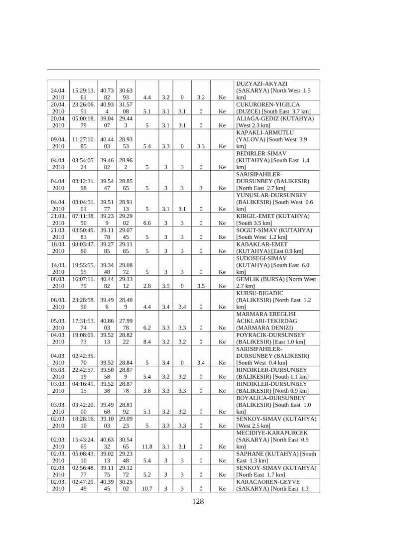
128

24.04.

2010

15:29:13.

61

40.73

82

30.63

93 4.4 3.2 0 3.2 Ke

DUZYAZI-AKYAZI

(SAKARYA) [North West 1.5

km]

20.04.

2010

23:26:06.

51

40.93

4

31.57

08 5.1 3.1 3.1 0 Ke

CUKUROREN-YIGILCA

(DUZCE) [South East 3.7 km]

20.04.

2010

05:00:18.

79

39.04

07

29.44

3 5 3.1 3.1 0 Ke

ALIAGA-GEDIZ (KUTAHYA)

[West 2.3 km]

09.04.

2010

11:27:10.

85

40.44

03

28.93

53 5.4 3.3 0 3.3 Ke

KAPAKLI-ARMUTLU

(YALOVA) [South West 3.9

km]

04.04.

2010

03:54:05.

24

39.46

82

28.96

2 5 3 3 0 Ke

BEDIRLER-SIMAV


km]

04.04.

2010

03:12:31.

98

39.54

47

28.85

65 5 3 3 3 Ke

SARISIPAHILER-

DURSUNBEY (BALIKESIR)

[North East 2.7 km]

04.04.

2010

03:04:51.

01

39.51

77

28.91

13 5 3.1 3.1 0 Ke

YUNUSLAR-DURSUNBEY

(BALIKESIR) [South West 0.6

km]

21.03.

2010

07:11:38.

50

39.23

9

29.29

02 6.6 3 3 0 Ke

KIRGIL-EMET (KUTAHYA)

[South 3.5 km]

21.03.

2010

03:50:49.

83

39.11

78

29.07

45 5 3 3 0 Ke


[South West 1.2 km]

18.03.

2010

08:03:47.

80

39.27

85

29.11

85 5 3 3 0 Ke

KABAKLAR-EMET

(KUTAHYA) [East 0.9 km]

14.03.

2010

19:55:55.

95

39.34

48

29.08

72 5 3 3 0 Ke

SUDOSEGI-SIMAV


km]

08.03.

2010

16:07:11.

79

40.44

82

29.13

12 2.8 3.5 0 3.5 Ke

GEMLIK (BURSA) [North West

2.7 km]

06.03.

2010

23:28:58.

90

39.49

6

28.40

9 4.4 3.4 3.4 0 Ke

KURSU-BIGADIC


km]

05.03.

2010

17:31:53.

74

40.86

03

27.99

78 6.2 3.3 3.3 0 Ke

MARMARA EREGLISI

ACIKLARI-TEKIRDAG

(MARMARA DENIZI)

04.03.

2010

19:08:09.

73

39.52

13

28.82

22 8.4 3.2 3.2 0 Ke

POYRACIK-DURSUNBEY

(BALIKESIR) [East 1.0 km]

04.03.

2010

02:42:39.

70 39.52 28.84 5 3.4 0 3.4 Ke

SARISIPAHILER-

DURSUNBEY (BALIKESIR)

[South West 0.4 km]

03.03.

2010

22:42:57.

19

39.50

58

28.87

9 5.4 3.2 3.2 0 Ke

HINDIKLER-DURSUNBEY

(BALIKESIR) [South 1.1 km]

03.03.

2010

04:16:41.

15

39.52

38

28.87

78 3.8 3.3 3.3 0 Ke

HINDIKLER-DURSUNBEY

(BALIKESIR) [North 0.9 km]

03.03.

2010

03:42:20.

00

39.49

68

28.81

92 5.1 3.2 3.2 0 Ke

BOYALICA-DURSUNBEY

(BALIKESIR) [South East 1.0

km]

02.03.

2010

18:28:16.

10

39.10

03

29.09

23 5 3.3 3.3 0 Ke


[West 2.5 km]

02.03.

2010

15:43:24.

65

40.63

32

30.54

65 11.8 3.1 3.1 0 Ke

MECIDIYE-KARAPURCEK


km]

02.03.

2010

05:08:43.

10

39.02

13

29.23

48 5.4 3 3 0 Ke

SAPHANE (KUTAHYA) [South

East 1.3 km]

02.03.

2010

02:56:48.

77

39.11

75

29.12

72 5.2 3 3 0 Ke


[North East 1.7 km]

02.03.

2010

02:47:29.

49

40.39

45

30.25

02 10.7 3 3 0 Ke

KARACAOREN-GEYVE


129

km]

02.03.

2010

01:48:31.

12 39.09

29.17

58 5 3.1 3.1 0 Ke

BASKONAK-SIMAV


km]

02.03.

2010

01:37:41.

80

39.11

85

29.10

77 5.1 3.3 3.3 0 Ke


[North West 2.1 km]

02.03.

2010

01:26:57.

46

39.08

75

29.17

1 5.4 3.1 3.1 0 Ke

BASKONAK-SIMAV


km]

02.03.

2010

01:21:36.

57

39.09

67

29.12

02 5.1 3.3 3.3 0 Ke


[South 0.7 km]

02.03.

2010

00:59:43.

08

39.13

47

29.09

4 6.4 4.3 0 4.3 Ke


[North East 1.4 km]

02.03.

2010

00:47:01.

08

39.10

37

29.05

47 5 3.1 3.1 3.1 Ke

GOKCELER-SIMAV


km]

02.03.

2010

00:36:10.

90 39.11

29.07

3 2 3.3 3.3 0 Ke


[South West 2.0 km]

18.02.

2010

17:48:09.

06

39.03

2

29.62

1 4 3.1 3.1 0 Ke

GOYNUK-GEDIZ (KUTAHYA)

[North West 2.6 km]

14.02.

2010

20:25:04.

77

39.73

7

30.54

73 2.9 3 3 0 Ke

ODUNPAZARI (ESKISEHIR)

[South East 3.8 km]

14.02.

2010

18:44:57.

61

40.83

83

27.82

38 4.9 3.1 3.1 0 Ke MARMARA DENIZI

11.02.

2010

10:21:01.

58

39.70

88

29.62

2 25.1 3 3 0 Ke

FINDICAK-DOMANIC


km]

10.02.

2010

17:26:13.

83

38.95

7

29.97

92 5.4 3 3 0 Ke

ALLIOREN-DUMLUPINAR


km]

08.02.

2010

02:46:05.

96

40.43

52

29.87

35 5 3.2 3.2 0 Ke

KARATEKIN-IZNIK (BURSA)

[South West 0.7 km]

07.02.

2010

17:21:32.

15

39.76

95

30.58

7 5 3.7 0 3.7 Ke

SULTANDERE-ODUNPAZARI

(ESKISEHIR) [North West 4.9

km]

04.02.

2010

16:05:59.

19

40.42

4

28.85

28 6 3 3 0 Ke

GEMLIK KORFEZI

(MARMARA DENIZI)

03.02.

2010

21:57:55.

00 40.4 28.85 9 3.5 0 3.5 Ke

KUMYAKA-MUDANYA

(BURSA) [North East 2.6 km]

30.01.

2010

12:28:10.

40 39.18

28.91

02 9.8 3 3 0 Ke

GUNEY-SIMAV (KUTAHYA)

[South West 0.8 km]

29.01.

2010

16:38:08.

77

39.49

68

28.90

2 5 3.1 3.1 0 Ke

DEMIRCILER-DURSUNBEY


km]

23.01.

2010

07:15:04.

04

39.96

12

28.78

15 4.2 3.2 3.2 0 Ke

OMERALTI-

MUSTAFAKEMALPASA

(BURSA) [South East 2.9 km]

20.01.

2010

20:53:09.

00

39.07

65

29.18

27 4.9 3.2 3.2 0 Ke

BASKONAK-SIMAV


km]

14.01.

2010

04:11:40.

05

40.76

5

31.63

6 5 3.2 3.2 0 Ke

YENIKOY- (BOLU) [South

West 1.2 km]

13.01.

2010

03:54:51.

54

40.63

78

28.76

9 10.6 3.4 0 3.4 Ke

ARMUTLU ACIKLARI-

YALOVA (MARMARA

DENIZI)

12.01.

2010

22:46:11.

19

40.62

58

29.01

25 6.7 3.2 3.2 0 Ke

SENKOY-CINARCIK

(YALOVA) [South East 0.8 km]

12.01.

2010

05:31:39.

23

40.47

97

28.14

9 7.6 3 3 0 Ke

BANDIRMA ACIKLARI-

BALIKESIR (MARMARA

DENIZI)

130

02.01.

2010

04:14:34.

66

40.85

35

29.28

6 9 3 3 0 Ke

TUZLA (ISTANBUL) [North

West 4.3 km]

01.01.

2010

21:01:21.

13 40.15

28.29

28 4.7 3 3 0 Ke

YOLAGZI-KARACABEY

(BURSA) [North West 1.9 km]

131

APPENDIX D

UNIFIED SOIL CLASSIFICATION SYSTEM

Table D 1: Unified Soil Classification System (based on Wagner, A.A. 1957) from Craig soil

mechanics

Name Group

Symbols

Laboratory Criteria

Fines

(%) Grading Plasticity Notes

Co

arse

gra

ined

(m

ore

th

an 5

0%

lar

ger

th

an 6

3 µ

m B

S o

r N

o.2

00

US

sie

ve

size

)

Gra

vel

s (m

ore

th

an 5

0%

of

coar

se f

ract

ion

of

gra

vel

siz

e)

Well graded

gravels,

sandy

gravels, with

little or no

fines

GW 0-5 Cu>4

1<Cz<3

Poorly

graded

gravels,

sandy

gravels, with

little or no

fines

GP 0-5

Not satisfying

GW

requirements

Silty gravels,

silty sandy

gravels

GM >12

Below A-

line or

Ip<4

Clayey

gravels,

clayey sandy

gravels

GC >12

Below A-

line or

Ip>7

San

ds

(mo

re t

han

50

%

of

coar

se f

ract

ion

of

san

d s

ize)

Well graded

sands,

gravelly

sands, with

little or no

fines

SW 0-5 Cu>6

1<Cz<3

Poorly

graded sands, SP 0-5 Not satisfying

SW

132

gravelly

sands, with

little or no

fines

requirements

Silty sands SM >12

Below A-

line or

Ip<4

Clayey sands SC >12

Below A-

line or

Ip>7

Fin

e g

rain

ed (

mo

re t

han

50

% s

mal

ler

than

63

µm

BS

or

No

.20

0 U

S s

iev

e si

ze)

Sil

ts a

nd

cla

ys

(liq

uid

lim

it l

ess

than

50

)

Inorganic

silts, silty or

clayey fine

sands, with

slight

plasticity

ML Use plasticity chart

Inorganic

clays, silty

clays, sandy

clays of low

plasticity

CL Use plasticity chart

Organic silts

and organic

silty clays of

low plasticity

OL Use plasticity chart

Sil

ts a

nd

cla

ys

(liq

uid

lim

it

gre

ater

th

an 5

0)

Inorganic

silts of high

plasticity

MH Use plasticity chart

Inorganic

clays of high

plasticity

CH Use plasticity chart

Organic

clays of high

plasticity

OH Use plasticity chart

Highly organic

soils

Peat and

other higgly

organic soils

Pt

133

APPENDIX E

DATASHEET OF THE CABLE USED IN FIELD

APPLICATION

GENERATION OF AN EARLY WARNING SYSTEM FOR …etd.lib.metu.edu.tr/upload/12619095/index.pdf · Fiber...

Documents

Transcript of GENERATION OF AN EARLY WARNING SYSTEM FOR …etd.lib.metu.edu.tr/upload/12619095/index.pdf · Fiber...