Generalized linear models - University of Helsinki Confluence · 2009-04-30 · Generalized linear...

Generalized linear models

Juha Karvanen

April 30, 2009

Contents

1 What is a generalized linear model? 51.1 Model . . . . . . . . . . . . . . . . . . . . . . . . . . . . . . . 51.2 Linear model . . . . . . . . . . . . . . . . . . . . . . . . . . . 51.3 Generalized linear model . . . . . . . . . . . . . . . . . . . . . 61.4 Motivating examples . . . . . . . . . . . . . . . . . . . . . . . 71.5 Link functions . . . . . . . . . . . . . . . . . . . . . . . . . . . 81.6 Confusing terminology . . . . . . . . . . . . . . . . . . . . . . 8

1.6.1 Generalized linear model (GLM) and general linearmodel (GLM) . . . . . . . . . . . . . . . . . . . . . . . 8

1.6.2 Names of X and Y . . . . . . . . . . . . . . . . . . . . 9

2 Generalized linear models in statistical software 102.1 Generalized linear models in R . . . . . . . . . . . . . . . . . . 102.2 Generalized linear models in SAS, Matlab and SPSS . . . . . . 12

3 Theory of generalized linear models 133.1 Notation . . . . . . . . . . . . . . . . . . . . . . . . . . . . . . 133.2 Model assumptions . . . . . . . . . . . . . . . . . . . . . . . . 133.3 Likelihood . . . . . . . . . . . . . . . . . . . . . . . . . . . . . 143.4 Canonical link . . . . . . . . . . . . . . . . . . . . . . . . . . . 153.5 Score function, observed information and expected informa-

tion (Fisher information) . . . . . . . . . . . . . . . . . . . . . 153.6 Estimation . . . . . . . . . . . . . . . . . . . . . . . . . . . . . 163.7 Deviance . . . . . . . . . . . . . . . . . . . . . . . . . . . . . . 173.8 Quasi-likelihood . . . . . . . . . . . . . . . . . . . . . . . . . . 18

1

Generalized linear models University of Helsinki, spring 2009

4 Modeling 194.1 Process of modeling . . . . . . . . . . . . . . . . . . . . . . . . 194.2 Residuals . . . . . . . . . . . . . . . . . . . . . . . . . . . . . 194.3 Nonlinear terms . . . . . . . . . . . . . . . . . . . . . . . . . . 204.4 Interactions . . . . . . . . . . . . . . . . . . . . . . . . . . . . 204.5 Hypothesis testing . . . . . . . . . . . . . . . . . . . . . . . . 21

4.5.1 Single test . . . . . . . . . . . . . . . . . . . . . . . . . 214.5.2 Multiple tests . . . . . . . . . . . . . . . . . . . . . . . 21

4.6 Model selection . . . . . . . . . . . . . . . . . . . . . . . . . . 224.7 Experimental and observational studies . . . . . . . . . . . . . 234.8 Missing data . . . . . . . . . . . . . . . . . . . . . . . . . . . . 234.9 Few words on independence . . . . . . . . . . . . . . . . . . . 23

5 Binary response 255.1 Representations of binary response data . . . . . . . . . . . . 255.2 Link functions for binary data . . . . . . . . . . . . . . . . . . 265.3 Odds and log-odds . . . . . . . . . . . . . . . . . . . . . . . . 265.4 Latent variables . . . . . . . . . . . . . . . . . . . . . . . . . . 275.5 Overdispersion . . . . . . . . . . . . . . . . . . . . . . . . . . 275.6 Non-existence of maximum likelihood estimates . . . . . . . . 275.7 Example: Switching measurements . . . . . . . . . . . . . . . 28

6 Count response 296.1 Representations of count response data . . . . . . . . . . . . . 296.2 Link functions for count data . . . . . . . . . . . . . . . . . . 306.3 Likelihood . . . . . . . . . . . . . . . . . . . . . . . . . . . . . 306.4 Offset . . . . . . . . . . . . . . . . . . . . . . . . . . . . . . . 316.5 Overdispersion . . . . . . . . . . . . . . . . . . . . . . . . . . 316.6 Example: Follow-up for cardiovascular diseases . . . . . . . . . 31

7 Nominal and ordinal response 327.1 Representations of nominal response data . . . . . . . . . . . . 327.2 Multinomial distribution . . . . . . . . . . . . . . . . . . . . . 337.3 Regression models for nominal and ordinal response . . . . . . 337.4 Proportional odds model . . . . . . . . . . . . . . . . . . . . . 347.5 Latent variable interpretation for ordinal regression . . . . . . 347.6 Nominal and ordinal response data in R . . . . . . . . . . . . 34

2


8 Positive response 358.1 Characteristics of positive response data . . . . . . . . . . . . 358.2 Gamma distribution . . . . . . . . . . . . . . . . . . . . . . . 358.3 Link functions for gamma distributed response . . . . . . . . . 368.4 Lognormal distribution . . . . . . . . . . . . . . . . . . . . . . 368.5 Inverse Gaussian distribution . . . . . . . . . . . . . . . . . . 368.6 Compound Poisson model . . . . . . . . . . . . . . . . . . . . 378.7 Weibull distribution . . . . . . . . . . . . . . . . . . . . . . . . 378.8 Pareto distribution . . . . . . . . . . . . . . . . . . . . . . . . 37

9 Time-to-event response 389.1 Representations of time-to-event data . . . . . . . . . . . . . . 389.2 Censoring and truncation . . . . . . . . . . . . . . . . . . . . . 389.3 Prospective and retrospective studies . . . . . . . . . . . . . . 399.4 Survival function and hazard function . . . . . . . . . . . . . . 399.5 Proportional hazards model . . . . . . . . . . . . . . . . . . . 41

10 Extensions and related models 4210.1 Beyond exponential family . . . . . . . . . . . . . . . . . . . . 4210.2 Dependent responses . . . . . . . . . . . . . . . . . . . . . . . 42

10.2.1 Generalized linear mixed models (GLMM) . . . . . . . 4210.2.2 Generalized estimation equations (GEE) . . . . . . . . 43

10.3 Nonlinear covariate effects . . . . . . . . . . . . . . . . . . . . 4310.3.1 Generalized additive models (GAM) . . . . . . . . . . 4310.3.2 Neural networks . . . . . . . . . . . . . . . . . . . . . . 43

10.4 Bayesian estimation of GLM . . . . . . . . . . . . . . . . . . . 44

3


Preface

This document contains short lecture notes for the course Generalized linearmodels, University of Helsinki, spring 2009. A more detailed treatment ofthe topic can be found from

• P. McCullagh and John A. Nelder, Generalized linear models. Secondedition 1989. Chapman & Hall.

• A. J. Dobson, An introduction to generalized linear models. Secondedition 2002. Third edition 2008. Chapman & Hall/CRC.

• lecture notes 2008. http://www.rni.helsinki.fi/~jmh/glm08/

• lecture notes 2005 (in Finnish). http://www.rni.helsinki.fi/~jmh/glm05/glm05.pdf.

4


1 What is a generalized linear model?

1.1 Model

Mathematical view: A statistical model is a set of probability distribu-tions on the sample space S. A parameterized statistical model is aparameter set Θ together with a function P : Θ → P (S), which assignsto each parameter point θ ∈ Θ a probability distribution Pθ on S. ABayesian model requires an additional component in the form of a priordistribution on Θ. [P. McCullagh (2002). What is a statistical model.The Annals of Statistics. Vol. 30, No. 5, 1225-1310.]

Applied view: Statistical model is a description of the probability distri-bution of random variables which can be assumed to represent a realworld phenomenon.

Which of these are statistical models?

a) X ∼ N(µ, σ2)

b) “The height of Finnish men follows a normal distribution.”

c)

L(θ,ψ) ∝n∏

i=1

pθ(gi)pψ(xi | gi)pθ(yi | gi, xi),

d) “The risk of smokers to die to cardiovascular diseases is about twice therisk of non-smokers.”

e) glm(y ~ x, family=binomial(link = "logit"), data=doseresponse)

1.2 Linear model

A simple linear model that describes the relationship of a single covariate xand a continuous response variable Y can be written as

Yi = α + βxi + ǫi, (1)

where α is the intercept term, β is the regression coefficient for X and ǫi

is an error term. Further assumptions are needed for the error term. For

5


instance, we may assume that the error terms are mutually independent andǫi ∼ N(0, σ2), i = 1, 2, . . . , n. A less restrictive assumption is to specify onlythe first two moments E(ǫi) = 0 and Var(ǫi) = σ2, i.e. the variance does notdepend on x. Note that in model (1), the error term ǫi is written explicitly.It is also possible to write the same model without explicitly specifying ǫi

E(Yi | xi) = µi = α + βxi. (2)

Model (2) tells on the expected value of Yi on the condition of x. As a such,model (2) does not specify how the values of Yi vary around the expectedvalue E(Yi | xi). Defining Var(Yi) = σ2 we obtain a model equivalent tomodel (1). If the variation of Yi is normally distributed, it can be alsowritten Yi ∼ N(α + βxi, σ

2).The linearity of linear model means linearity respect to the parameters.

In other words, the model µi = α + βx3i is also a linear model.

1.3 Generalized linear model

The linear model (2) can be transformed to a generalized linear model byreplacing µi by g(µi)

g(µi) = α + βxi = ηi, (3)

where g is a real-valued monotonic and differentiable function called linkfunction and the term ηi is called linear predictor. In the other words, µi isthe expected value of the response, ηi is a linear combination of the covariatesand g() defines the relationship between µi and ηi. Because g() is monotonic,the relationship of µi and ηi is also monotonic. With the inverse of g() wemay write

µi = g−1(ηi), (4)

which provides an alternative way to define GLM. Linear model is a specialcase of GLM where g(µi) = µi.

With multiple covariates the GLM is defined as

g(µi) =

p∑

j=1

βjxij . (5)

The assumptions of the GLM are given in Section 3.

6


Note that GLM is different from applying a nonlinear transformation toresponse variable. In GLM, the nonlinear transformation is applied to theexpected value of the response.

Variance is defined by the variance function V that specifies the varianceof Yi as a function µi

Var(Yi) ∝ V (µi). (6)

1.4 Motivating examples

Generalized linear models are needed because linear models are not appro-priate for all situations. In linear model it is implicitly assumed that theresponse can be have all real values, which is not the case in many practicalsituations. Examples:

• The number of hospital visits in a certain year for an individual is acount response that can have values 0, 1, 2, . . ..

• Monthly alcohol consumption (liters of absolute alcohol) for an indi-vidual is a nonnegative response that has zeroes for some individuals.

• Gamma-glutamyltransferase (GGT) measured from serum blood is apositive response.

• Daily rainfall is a nonnegative response.

• Presence or absence of a voltage peak in switching measurements ofsuperconducting Josephson Junctions is a binary response.

• Fatality (fatal/non-fatal) of myocardial infarction (heart attack) is abinary response.

• Level of education (primary school, secondary school, B.Sc., M.Sc.,PhD) is an ordinal response.

• The date of an event of coronary heart disease measured for a cohortof people is a time-to-event (or survival) response.

There are also situations where a linear model may be suitable althoughstrictly speaking the response has an inappropriate distribution.

• Height of an adult is positive but can be modeled by linear modelbecause all values are far from zero.

7


• The daily number of customers in a big supermarket is actually a countresponse but could be modeled by linear model because all values arefar from zero and the number of possible values of the response is high.

1.5 Link functions

The choice of the link function g() depends on the data, especially on thetype of the response variable. If the response is a count, i.e. an integer,log-link g(µi) = log(µi) may be used. Log-link leads multiplicative model

µi = exp(ηi) = eβ1xi1eβ2xi2 · · · eβpxip (7)

If the response Yi is a binary variable with possible values 0 and 1, it holds

µi = E(Yi) = 1 · P (Yi = 1) + 0 · P (Yi = 0) = P (Yi = 1). (8)

The logit-link

g(µi) = logit(µi) = log

(

µi

1 − µi

)

(9)

is maybe the most typical choice for binary response data. For positivecontinuous responses typical link functions are inverse link

µ−1i = ηi (10)

and inverse-squared linkµ−2

i = ηi. (11)

1.6 Confusing terminology

1.6.1 Generalized linear model (GLM) and general linear model(GLM)

Unfortunately, the acronym GLM is sometimes used for general linear model.General linear model is a linear model. The word ‘general’ is used to indicatethat the response Y may be multivariate and the covariates may include bothcontinuous and categorical variables. In SAS, PROC GLM fits a generallinear model, not a generalized linear model.

8


1.6.2 Names of X and Y

In different applications X and Y have various names that sometimes mightbe confusing. Examples are given below. Some of the names are synonymsand some have special emphasis in certain applications. Particularly, theterms ‘independent variable’ and ‘dependent variable’ may cause a confusion.

Names of X

• covariate

• explanatory variable

• factor

• risk factor

• exposure (variable)

• design variable

• controlled variable

• carrier variable

• regressor

• predictor

• input

• determinant

• ∗independent variable

Names of Y

• response

• explained variable

• outcome

• responding variable

• regressand

• experimental variable

• measured variable

• output

• ∗dependent variable

9


2 Generalized linear models in statistical soft-

ware

2.1 Generalized linear models in R

In R (www.r-project.org) generalized linear models can be fitted usingfunction glm. The syntax isglm(formula, family = gaussian, data, weights, subset, na.action,

start = NULL, etastart, mustart, offset, control = glm.control(...),

model = TRUE, method = "glm.fit", x = FALSE, y = TRUE, contrasts

= NULL, ...)

ArgumentsSome important arguments are

formula an object of class ”formula” (or one that can be coerced to thatclass): a symbolic description of the model to be fitted.

family a description of the error distribution and link function to be usedin the model. This can be a character string naming a family function,a family function or the result of a call to a family function.

data an optional data frame, list or environment (or object coercible byas.data.frame to a data frame) containing the variables in the model.weights] an optional vector of weights to be used in the fitting process.

subset an optional vector specifying a subset of observations to be used inthe fitting process.

offset can be used to specify an a priori known component to be included inthe linear predictor during fitting. This should be NULL or a numericvector of length either one or equal to the number of cases. One ormore offset terms can be included in the formula instead or as well,and if both are specified their sum is used. See model.offset.

control a list of parameters for controlling the fitting process.

OutputAs an output an object of class “glm” is returned. A glm object is a list thatcontains the following components among the others:

10


coefficients a named vector of coefficients

fitted.values the fitted mean values, obtained by transforming the linearpredictors by the inverse of the link function.

deviance up to a constant, minus twice the maximized log-likelihood. Wheresensible, the constant is chosen so that a saturated model has deviancezero.

aic Akaike’s An Information Criterion, minus twice the maximized log-likelihood plus twice the number of coefficients (so assuming that thedispersion is known).

null.deviance The deviance for the null model, comparable with deviance.

iter the number of iterations of IWLS used.

df.residual the residual degrees of freedom.

df.null the residual degrees of freedom for the null model.

converged logical. Was the IWLS algorithm judged to have converged?

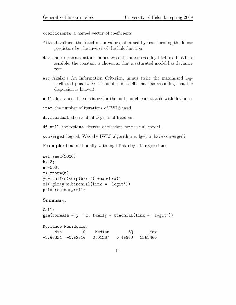
Example: binomial family with logit-link (logistic regression)

set.seed(3000)

b<-3;

n<-500;

x<-rnorm(n);

y<-runif(n)<exp(b*x)/(1+exp(b*x))

m1<-glm(y~x,binomial(link = "logit"))

print(summary(m1))

Summary:

Call:

glm(formula = y ~ x, family = binomial(link = "logit"))

Deviance Residuals:

Min 1Q Median 3Q Max

-2.66224 -0.53516 0.01267 0.45869 2.62460

11


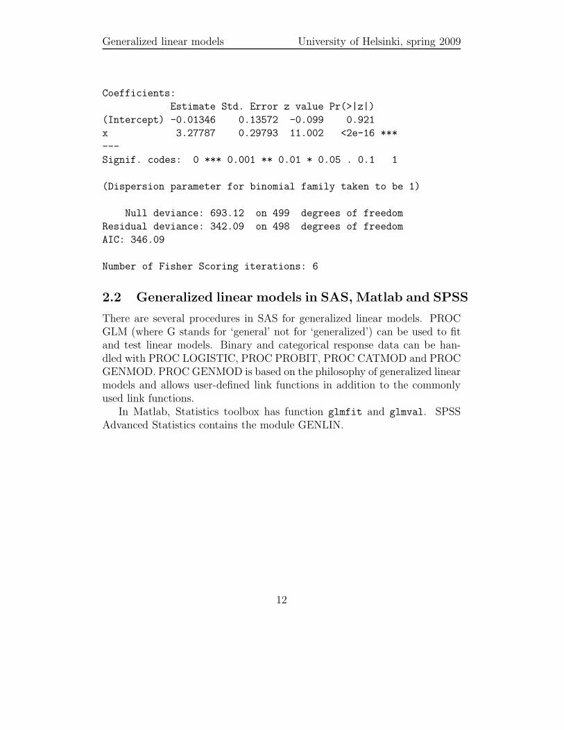
Coefficients:

Estimate Std. Error z value Pr(>|z|)

(Intercept) -0.01346 0.13572 -0.099 0.921

x 3.27787 0.29793 11.002 <2e-16 ***

---

Signif. codes: 0 *** 0.001 ** 0.01 * 0.05 . 0.1 1

(Dispersion parameter for binomial family taken to be 1)

Null deviance: 693.12 on 499 degrees of freedom

Residual deviance: 342.09 on 498 degrees of freedom

AIC: 346.09

Number of Fisher Scoring iterations: 6

2.2 Generalized linear models in SAS, Matlab and SPSS

There are several procedures in SAS for generalized linear models. PROCGLM (where G stands for ‘general’ not for ‘generalized’) can be used to fitand test linear models. Binary and categorical response data can be han-dled with PROC LOGISTIC, PROC PROBIT, PROC CATMOD and PROCGENMOD. PROC GENMOD is based on the philosophy of generalized linearmodels and allows user-defined link functions in addition to the commonlyused link functions.

In Matlab, Statistics toolbox has function glmfit and glmval. SPSSAdvanced Statistics contains the module GENLIN.

12


3 Theory of generalized linear models

3.1 Notation

The observed data set (y,X) contains n observations of 1 + p variables

y =(

y1 y2 . . . yn

)T(12)

X =

x11 x12 . . . x1p

x21 x22 . . . x2p...

......

xn1 xn2 . . . xnp

. (13)

Variable y is the response variable and variables x1, x2, . . . xp are explanatoryvariables or covariates. The observed value yi is treated as a realization ofa random variable Yi. In experimental setup, the explanatory variables havefixed values set by the experimenter. In observational setup, the value xij

can be understood to be a realization of a random variable Xij but whendistribution of Yi is considered xij is taken as fixed.

The parameters include the regression coefficients

β =(

β1 β2 . . . βp

)T, (14)

the linear predictors

η =(

η1 η2 . . . ηn

)T, (15)

the expected responses

µ =(

µ1 µ2 . . . µn

)T, (16)

and the canonical parameters

θ =(

θ1 θ2 . . . θn

)T. (17)

3.2 Model assumptions

1. The distribution of Yi belongs to the exponential family. For the expo-nential family, the density function can be presented in the form

fYi(yi; θi, φ) = exp

(

ai(yiθi − b(θi))

φ+ c(yi, φ/ai)

)

, (18)

where

13


• θi, i = 1, . . . , n are unknown parameters (canonical parameters),

• φ is the dispersion parameter (scale parameter) that can be knownor unknown,

• ai, i = 1, . . . , n are known prior weights of each observation and

• b() and c() are known functions. The first derivative b′() is mono-tonic and differentiable.

2. Random variables Y1, Y2, . . . , Yn are mutually independent.

3. The expected value µi = E(Yi) depends on linear predictor ηi =∑p

j=1 xijβj

through monotonic and differentiable link function g

g(µi) = ηi. (19)

For instance, normal, binomial, Poisson and gamma distributions belongto the exponential family. For exponential family (18) it holds

E(Yi) = b′(θi) = µi (20)

and

Var(Yi) =b′′(θi)φ

ai

=V (µi)φ

ai

. (21)

As shown in section 3.8, the assumption on the exponential family can berelaxed.

3.3 Likelihood

The log-likelihood of y1, . . . , yn from an exponential family with known dis-persion parameter φ can be written

l(θ1, . . . , θn; φ, a,y) =n∑

i=1

(

ai(yiθi − b(θi))

φ+ c(yi, φ/ai)

)

(22)

If there are no restrictions for parameters θ1, . . . , θn, the model is saturated,i.e. it has as many parameters as there are observations. In a GLM, theparameters θ1, . . . , θn depend on X and the parameters β1, . . . , βp throughfunctions b() and g()

p∑

j=1

βjxij = ηi = g(µi) = g(b′(θi)). (23)

14


Therefore, the log-likelihood can be written also a function of the parametersµ1, . . . , µn or as a function of the parameters β1, . . . , βp

l(µ1, . . . , µn; φ, a,y) =n∑

i=1

(

ai(yi(b′)−1(µi) − b((b′)−1(µi)))

φ+ c(yi, φ/ai)

)

, (24)

l(β1, . . . , βp; φ, a,y) =n∑

i=1

(

ai(yi(b′)−1(g−1(

∑pj=1 βjxij)) − b((b′)−1(g−1(

∑pj=1 βjxij))))

φ+ c(yi, φ/ai)

)

.

(25)

3.4 Canonical link

The link function for which it holds ηi = g(µi) = θi is called canonical link.Because µi = b′(θ), it follows g = (b′)−1. The use of canonical link functionsimplifies calculations but this alone does not justify the use of canonicallink. The link function should be selected on the basis of the data and priorknowledge on the problem.

3.5 Score function, observed information and expectedinformation (Fisher information)

The partial derivative of log-likelihood with respect to some parameter iscalled score or score function. In the case of the exponential family (22) we

15


obtain

∂l

∂θi=

ai(yi − b′(θi))

φ, (26)

∂l

∂µi=

∂l

∂θi

∂θi

∂µi=


φ

1

V (µi), (27)

∂l

∂ηi=

∂l

∂θi

∂θi

∂µi

∂µi

∂ηi=


φ

1

V (µi)(g−1)′(ηi), (28)

∂l

∂βj

=n∑

i=1

∂l

∂θi

∂θi

∂µi

∂µi

∂ηi

∂ηi

∂βj

=n∑

i=1


φ

1

V (µi)(g−1)′(ηi)xij =

1

φ

n∑

i=1

ai(yi − µi(β))xij

V (µi(β))g′(µi(β))(29)

where the notation µi(β) emphasizes the fact that µi depends on β.The observed information is the negative of the matrix of second order

partial derivatives of log-likelihood

J(β,y) = −∂2l(β,y)

∂β2 =

−∑n

i=1∂2l(β,yi)

∂β21

. . . −∑n

i=1∂2l(β,yi)∂β1∂βp

.... . .

...

−∑n

i=1∂2l(β,yi)∂βp∂β1

. . . −∑n

i=1∂2l(β,yi)∂βp∂βp

(30)

and the Fisher information or expected information is the expected value ofobserved information

I(β) = EY(J(β,Y)) =

n∑

i=1

EYi(J(β, Yi)) = −

n∑

i=1

E

(

∂2l(β, Yi)

∂β2

)

. (31)

3.6 Estimation

The maximum likelihood estimate for β is obtained by solving score equations

∂l(β,y)

∂β= 0. (32)

Usually the estimation requires numerical methods. Traditionally, the maxi-mum likelihood estimation is carried out with Fisher scoring (also called iter-ative weighted least squares) which is a modification of the Newton-Raphsonalgorithm.

16


In Newton-Raphson update rule

β̂(t+1)

= β̂(t)

+ J−1∂l(β,y)

∂β(33)

the observed information J is replaced by the expected information I. Aftersome algebra, this leads to the update formula

β̂(t+1)

= (XTW(t)X)−1XTW(t)z(t), (34)

where

W(t) =

w(t)1

. . .

w(t)1

, (35)

w(t)i =

ai[

g′(

µi(β̂(t)

))]2

V(

µi(β̂(t)

))

, (36)

z(t) = (z(t)1 . . . z(t)

n )T (37)

z(t)i = ηi(β̂

(t)) + (yi − µi(β̂

(t)))g′

(

µi(β̂(t)

))

. (38)

It can be seen that the updating rule depends on the distribution of Yi onlythrough the variance function V .

When the maximum likelihood estimator β̂ exists, it is consistent andasymptotically normal with expected value β and covariance matrix φ(XTWX)−1.

The dispersion parameter φ can estimated by the deviance (see Sec-tion 3.7) estimator

φ̂ =D

n − p(39)

or the moment estimator

φ̂ =1

n − p

n∑

i=1

ai(yi − µi(β̂))2

V (µi(β̂)). (40)

3.7 Deviance

Deviance is defined as

D(y; µ̂) = 2φ(l(y;y) − l(µ̂;y)) (41)

17


where l(y;y) is the log-likelihood of the saturated model (full model). In thesaturated model, the number of parameters equals the number of observationsand likelihood obtains its maximum for the model class. Scaled deviance isdefined as

D∗(y; µ̂) =D(y; µ̂)

φ(42)

As seen in Section 4.5, deviance is closely related to the likelihood ratio test.

3.8 Quasi-likelihood

GLMs allow defining the variance function independently from the link func-tion. The assumption that the distribution of Yi belongs to the exponentialfamily can be replaced by an assumption that concerns only the variance ofYi

Var(Yi) =φV (µi)

ai. (43)

Parameters can be estimated maximizing quasilikelihood

Q(β;y) =1

φ

n∑

i=1

∫ µi

yi

a(yi − t)

V (t)dt. (44)

The form of quasilikelihood function is chosen so that partial derivatives

∂Q(β;y)

∂βj

=1

φ

n∑

i=1

ai(yi − µi(β))xij

V (µi(β))g′(µi(β)). (45)

are similar to the partial derivatives of likelihood function and consequentlythe parameters can be estimated by Fisher scoring.

18


4 Modeling

4.1 Process of modeling

1. Study design

2. Data collection

3. Selection of model class

4. Estimation

5. Model checking

6. Conclusions

7. Reporting

4.2 Residuals

Residuals can be used to check the model fit. For GLMs different kind ofresiduals can be defined:

Raw residuals (response residuals)

ri = yi − µ̂i (46)

Pearson residuals

rP,i =yi − µ̂i

√

V (µ̂i)/ai

(47)

whose squared sumn∑

i=1

r2P,i = X2 (48)

is the Pearson chi-squared goodness-of-fit statistic.

Deviance residualsrD,i = sign(yi − µ̂i)

√

di, (49)

where

di = 2ai (yi (θi(yi) − θi(µ̂i)) − b (θi(yi)) + b (θi(µ̂i))) . (50)

19


The deviance is the squared sum of the deviance residuals

n∑

i=1

r2D,i = D(y; µ̂) (51)

Anscombe residuals where yi’s and µi’s are transformed so that the resid-uals become approximately normally distributed.

In R, method residuals for class glm can compute raw, Pearson and de-viance residuals.

Influential observations can be identified, for instance, by calculating dif-ferences

∆iβ̂ = β̂ − β̂(i)(52)

where β̂(i)

is estimated from data without observation i.

4.3 Nonlinear terms

GLMs allow inclusion of known transformations of the covariates as far asthe linear predictor ηi can be presented as a sum of transformed covariates.For instance, the design matrix may be defined as

X =

1 x11 x211 x3

11...

......

...1 xn1 x2

n1 x3n1

. (53)

to fit a GLM with a third order polynomial for covariate x1.

4.4 Interactions

Interaction terms are nonlinear transformations of two or more covariates.The type of interaction can synergistic (the joint effect is stronger than theadditive effect) or antagonist (the joint effect is weaker than the additiveeffect). It is usually a bad idea to include interaction terms without thecorresponding main effects.

20


4.5 Hypothesis testing

4.5.1 Single test

The test of hypothesis

H0 : βj = 0

H1 : βj 6= 0

for a certain regression coefficient βj of a GLM can be based on the likelihoodratio test

Λ =sup{L(β1, . . . , βp;y) : βj = 0}

sup{L(β1, . . . , βp;y)} (54)

Using log-likelihoods the test statistic can be written

−2 log Λ = 2(l(β̂;y) − l(β̂0;y)) (55)

where β̂ = β̂1, . . . , β̂p and β̂0 = β̂1, . . . , βj = 0, . . . , β̂p are the maximumlikelihood estimates under the two models. The statistic −2 log Λ followsasymptotically χ2

1 distribution The test can written also in terms of deviance

−2 log Λ =D(y; β̂0) − D(y; β̂)

φ. (56)

The likelihood ratio test for more than one parameter is similar but thetest statistic follows asymptotically χ2 distribution with degrees of freedomequal to the difference in dimensionality of β and β0. If the dispersion pa-rameter is not known, the test statistics

D(y; β̂0) − D(y; β̂)

φ̂(p − q)(57)

where q is the dimensionality of β follows asymptotically F-distributionFp−q,n−p.

4.5.2 Multiple tests

Let p1, p2, . . . , pm be the nominal p-values from m tests. Family-wise errorrate (FWER) is the probability that at least one true null hypothesis is falselyrejected. Several approaches for controlling FWER exist: a simple approach

21


is the Bonferroni correction where the nominal p-values are compared tothe α/m where α is the significance level. If the tests are dependent, theBonferroni correction is too conservative and the actual significance level issmaller than α.

False discovery rate (FDR) is the expected proportion of incorrectly re-jected null hypothesis in a set of hypotheses. The FDR analysis has beenused e.g. in genome wide association (GWA) studies where the number oftests can be one million.

4.6 Model selection

Multiple models. Competing models are fitted and the estimated modelparameters are reported for each model. The properties of the modelsare discussed. This is actually not a formal model selection method buta commonly used practical approach to the problem. The approach isfeasible only if the number of the competing models is small.

Likelihood ratio test can be used to compare nested models.

Stepwise regression. In forward selection, the procedure starts with anull model and covariates are added one by one. The procedure con-tinues until the newly added covariate does not improve the model.The improvement of the model defined e.g. by the p-value of thelikelihood ratio test. In backward elimination, the procedure startswith the full model and covariates are removed one by one. The pro-cedure continues until the removal of a covariate makes the modelworse. The lasso (least absolute shrinkage and selection operator,http://www-stat.stanford.edu/~tibs/lasso.html) can be under-stood as a modernized version of stepwise regression (not based on like-lihood). Stepwise methods cannot guarantee that the best model willbe selected. Automated methods should not replace careful thinking.

Information criteria: Akaike information criterion (AIC), Bayesian infor-mation criterion (BIC), Bayes factor, crossvalidation, etc. AIC andBIC are straightforward to compute

AIC = −2l(β;y) + 2p,

BIC = −2l(β;y) + p log(n),

22


where p is the number of parameters in the model. The model withsmallest value of AIC (or BIC if that is used) will be considered the best.Both AIC and BIC penalize models for a higher number of parameters.In BIC, the penalty depends also on the number of observations.

4.7 Experimental and observational studies

Experimental data origin from data generating mechanism where the exper-imenter selects the values of some variables. In observational data, all valuesare recorded as observed. The same GLMs can be used for both types ofdata. The analysis follows the same lines but the interpretation of the re-sults may differ. In general, only experimental data allows causal inference.With observational data, the possibility of confounders and alternative causalexplanations must be accounted.

4.8 Missing data

Usually there are missing observations in real world data. A statistician hasthe following options:

Ignore the missing observations and analyze only the complete cases. Thisis applicable if only few observations are missing.

Impute the missing values. Multiple imputation is preferred over single im-putation. The challenges lie in the definition of the imputation model.

Model the data. The likelihood becomes an integral over the missing values.The results are sensitive to model misspecification and estimation mayrequire a lot of computational resources.

4.9 Few words on independence

Term “independence” may have different meanings depending on the context.In statistics, the term refers to independence of events or to independence ofrandom variables. Events A and B are independent if

P (A and B) = P (A)P (B). (58)

or equivalently, using conditional probabilities

P (A |B) = P (A) (59)

23


orP (B |A) = P (B). (60)

Random variables X and Y are independent (marked X ⊥⊥ Y ) if

FX,Y (X, Y ) = FX(X)FY (Y ). (61)

The term “linear independence of random variables” is sometimes used toindicate that the random variables are uncorrelated but this usage is notrecommended. In general, zero correlation does not imply independence.

In linear algebra, linear independence of a family of vectors means thatnone of the vectors can be presented as a linear combination of the othervectors. A matrix whose columns are linearly independent has full rank.

The concept of conditional independence is important when causality isconsidered. Random variables X and Y are independent on the condition of

Z (notation X⊥⊥Z Y or X ⊥⊥ Y |Z may be used) when

FX,Y |Z(X, Y |Z) = FX |Z(X |Z)FY |Z(Y |Z) (62)

or equivalentlyFX, |Y,Z(X | Y, Z) = FX |Z(X |Z). (63)

24


5 Binary response

5.1 Representations of binary response data

In binary response data, the response Yi has two possible values, for instance,0 and 1. Binary response data can be presented in different formats:

Data matrixx y

250 0250 1350 1300 0250 0300 1

......

Weighted data matrixx y frequency

250 0 23250 1 12300 1 21300 0 19350 0 7350 1 13

Frequency table (crosstabulation)Y = 0 Y = 1

x = 250 23 12x = 300 21 19x = 350 7 13

The response Yi can be either a Bernoulli random variable (binary re-sponse) or a sum of Bernoulli random variable (binomial response). In thelatter case, the observational units with the identical covariate values belongto the same covariate class. For the ith covariate class mi binary responsesare recorded and the number of responses 1 is denoted by Ki. The binomial

25


response is defined

Yi =Ki

mi. (64)

5.2 Link functions for binary data

If the possible values of Yi are 0 and 1, it holds

P (Yi = 1) = E(Yi) = g−1(ηi), (65)

where the possible values of the inverse link function g−1() belong to theinterval (0, 1). Any cumulative distribution function defines the inverse of alink function. The commonly used link functions are the logit link

g(µi) = logit(µi) = log

(

µi

1 − µi

)

, (66)

the probit linkg(µi) = probit(µi) = Φ−1(µi), (67)

where Φ−1 is the inverse of cumulative distribution function (cdf) of thestandard normal distribution and the complementary log-log link

g(µi) = cloglog(µi) = log(− log(1 − µi)). (68)

5.3 Odds and log-odds

It is often interesting to compare the estimated responses for different valuesof covariates. Denote

pA = P (Yi = 1 | ηA) (69)

pB = P (Yi = 1 | ηB) (70)

where ηA and ηB are the linear predictors for certain values of covariates.Now the odds ratio is defined as

pA/(1 − pA)

pB/(1 − pB(71)

and the logarithm of the odds ratio becomes

log

(

pA/(1 − pA)

pB/(1 − pB

)

= log

(

pA

1 − pA

)

− log

(

pB

1 − pB

)

= logit(pA)− logit(pB),

(72)

26


which in the case of logit link simplifies

logit(pA) − logit(pB) = ηA − ηB. (73)

5.4 Latent variables

Consider an example where the effectiveness of an insecticide to mosquitos isstudied. Mosquitos have different resistance to the insecticide. A mosquitodies (Y = 1) if the amount of insecticide x is higher than a threshold valueT , which varies in the population. Because T cannot be directly measured,it is called latent variable. If T follows the normal distribution with mean−α/β and variance 1/β2 we obtain for a mosquito randomly chosen from thepopulation

P (Y = 1) = P (T ≤ x) = Φ

(

x − (−α/β)

1/β

)

= Φ(α + βx). (74)

In other words, the use of normal distributed latent variable led to the probitmodel. If T follows logistic distribution, we will end up with the logisticmodel. If T follows Gumbel distribution, we will end up with the GLM withcloglog link.

5.5 Overdispersion

Overdispersion means that the variance in the data is greater than the vari-ance assumed in the model. The sum of independent Bernoulli random vari-ables

K = Y1 + Y2 + . . . + Ym (75)

follows binomial distribution K ∼ Bin(m, µ) where E(Yi) = µ. It followsthat Var(K) = mµ(1 − µ). In real world datasets, however, the assumptionof independence is often unrealistic and Var(K) > mµ(1− µ). This is calledoverdispersion.

5.6 Non-existence of maximum likelihood estimates

Maximum likelihood estimates do not exist if the data can be perfectly sep-arated on the basis of covariate values, for example, response 1 is alwaysobtained if x > 100 and response 0 is always obtained if x < 100.

27


5.7 Example: Switching measurements

The Josephson junction (JJ) circuits are important non-linear componentsof superconducting electronics. The strong dependence of the physical pa-rameters of JJ circuits as function of changes in environmental variables, forinstance, temperature, electric noise, and magnetic field makes the JJ circuitsto have several applications as ultra-sensitive sensors. Moreover, certain JJcircuits are promising candidates for realization of quantum computation.An experiment called switching measurement is a common way to probethe properties of a JJ circuit sample. In the experiment, sequences of cur-rent pulses are applied to the sample, while the voltage over the structureis monitored. Switching measurements are ideal applications for design ofexperiments in sense that the underlying parametric model for the switchingdynamics of a single JJ can be derived directly from the laws of physics.With quantum mechanical arguments, it can be shown that the probabilityof the voltage response can be approximated by

P (Y = 1) = 1 − e− exp(ax+b)

P (Y = 0) = e− exp(ax+b), (76)

where a and b are unknown parameters to be estimated and x is the heightof the current pulse. It follows that the measurement data can be modeledby a GLM with cloglog link function.

In an experiment carried out in Low Temperature Laboratory, HelsinkiUniversity of Technology in August 2005, a sample consisting of aluminium–aluminium oxide–aluminium Josephson junction circuit in a dilution refrig-erator at 20 millikelvin temperature was connected to computer controlledmeasurement electronics in order to apply the current pulses and record theresulting voltage pulses. The resistance of the sample at room temperaturesuggested that a pulse of 300 nA always causes a switching (response 1),which gave the upper limit for the initial estimation. The lower limit for theinitial estimation, 200 nA was roughly estimated from the dimensions of theJosephson junction by an experienced physicist. The experiment was carriedout sequentially so that the height of pulse for stage was determined usingthe measurement data recorded on the earlier stages.

28


6 Count response

6.1 Representations of count response data

In the count data, the possible values the response variable Yi are integers0, 1, 2, . . .. In practical situations there is sometimes an upper limit for Yi

but this can be ignored if E(Yi) is far below the the upper limit. It is oftenassumed that the counted events arise from a Poisson process whose intensitydepends on the covariates.

When the number of events for each individual are observed, the datacan be presented in the form of data matrix

x1 x2 y250 A 7250 A 1350 B 1300 A 0250 B 8300 B 3

......

...

or weighted data matrixx1 x2 y frequency

250 A 0 4250 A 1 2250 A 3 1250 B 0 4250 B 1 5250 B 2 3250 B 3 2300 A 0 6

......

......

When the number of events are observed only for each covariate class, thedata can be presented in the form of frequency table (crosstabulation)

x2 = A x2 = Bx1 = 250 23 12x1 = 300 21 19x1 = 350 7 13

29


6.2 Link functions for count data

Count data can be modeled by a GLM with the logarithmic link function

log(µi) =

p∑

j=1

βjxij . (77)

These models are also called Poisson regression or log-linear models.

6.3 Likelihood

The log-likelihood Poisson distributed response has the form

l(y;β) =n∑

i=1

yi log(µi) − µi − log(yi!) =

n∑

i=1

(

p∑

j=1

βjxijyi − exp

(

p∑

j=1

βjxij

)

− log(yi!)

)

. (78)

Example: Full likelihood for missing data Count response yi, con-tinuous covariate xi1 and binary covariate xi2 are recorded for the samplei = 1, 2, . . . , 1000. yi and xi1 are observed for all i but xi2 is missing fori = 1, 2, . . . , 250. We can assume that the values xi2 are missing at random(MAR), i.e. the missingness does not depend on the unobserved value itselfbut it may depend on the observed response or on the other covariate. Thefull likelihood for the data can be written

L(y; β1, β2) =250∏

i=1

(

p(Xi2 = 1)p(xi1|Xi2 = 1)exp(β1xi1 + β2)

yi exp(− exp(β1xi1 + β2))

yi!+

p(Xi2 = 0)p(xi1|Xi2 = 0)exp(β1xi1)

yi exp(− exp(β1xi1))

yi!

)

×1000∏

i=251

p(xi2)p(xi1|xi2)exp(β1xi1 + β2xi2)

yi exp(− exp(β1xi1 + β2xi2))

yi!. (79)

In order to calculate this likelihood we need to specify the marginal distri-bution p(x2) and the conditional distribution p(x1|x2). This may requirespecification of some additional parameters that are considered as nuisanceparameters and are estimated together with the parameters of interest β1

and β2.

30


6.4 Offset

The intensity of a process is defined in the form events/time and the observednumber of events depends on the system has been followed up. In the GLM,the time is taken into account adding an offset term

log(µi) =

p∑

j=1

βjxij + log(ti), (80)

where ti is the offset, i.e. the follow-up time or the time under exposure. Theregression coefficient of the offset is fixed to 1. In R, this can done with themodel term offset.

6.5 Overdispersion

For the Poisson distribution the variance is equal to expected value. In real-world data, it is common that the observed variance is higher, i.e. there isoverdispersion.

6.6 Example: Follow-up for cardiovascular diseases

Cohort studies are important in epidemiological research. A population co-hort represents the population of specified age range living in a certain geo-graphical area. The FINRISK cohort 1982 consists of men and women whowere 25-64 years old at baseline year 1982 (the beginning of the follow-up).The cohort has been followed up for deaths and fatal and non-fatal eventsof cardiovascular diseases until the end of year 2006. The example data setcontains the number of recorded events grouped by year, age group, sex andarea (Eastern Finland / Western Finland). The number of events should beconsidered in proportion to the person years of follow-up.

31


7 Nominal and ordinal response

7.1 Representations of nominal response data

Data matrixx y

250 A250 C350 C300 A250 B300 B

......

Weighted data matrixx y frequency

250 A 23250 B 12250 C 4300 A 21300 B 19300 C 7350 A 7350 B 13350 C 3

Frequency table (crosstabulation)Y =′ A′ Y =′ B′ Y =′ C ′

x = 250 23 12 4x = 300 21 19 7x = 350 7 13 3

In nominal response data, the response is one of the categories. In ordinalresponse data, the categories have a natural order. Binomial response is aspecial case of both nominal and ordinal response.

When there are more than two categories, nominal and ordinal responsehave a multivariate nature. For the ith covariate class mi responses arerecorded and the number of responses in the categories 1, 2, . . . , Q is denoted

32


by a vector(

Ki1Ki2 . . .KiQ

)

. The response is then defined as vector

Yi =(

Ki1

mi

Ki2

mi. . .

KiQ

mi

)

. (81)

7.2 Multinomial distribution

Multinomial distribution is a generalization of binomial distribution in thecase when there are more than two categories

fi(ki1, ki2, . . . , kiQ; mi, πi1, πi2, . . . , πiQ) =mi!

ki1!ki2! · · · kiQ!πki1

i1 πki2

i2 · · ·πkiQ

iQ ,

(82)where πiq’s are category probabilities for which

∑Qq=1 πiq = 1.

Multinomial distribution does not belong to the exponential family de-fined in equation (18) but it can derived from the Poisson distribution. LetK1, K2, . . . , KQ be independent Poisson distributed random variables withmeans λ1, λ2, . . . , λQ. The sum m = K1 +K2 + . . .+KQ is a random variablethat follows Poisson distribution with the mean λ = λ1 +λ2 + . . .+λQ. Thenthe conditional distribution

f(k1, k2, . . . , kQ; m) =

∏Qq=1 λ

kqq e−λq

kq

/

λme−λ

m=

(

λ1

λ

)k1(

λ2

λ

)k2

· · ·(

λQ

λ

)kQ m!

k1!k2! · · · kQ!(83)

has the form of the multinomial distribution.

7.3 Regression models for nominal and ordinal response

There are alternative ways to parameterize regression models for nominaland ordinal response. For nominal response data, one of the categories istypically chosen as the reference category and the model has form

log

(

πiq

πi1

)

= β0q +

p∑

j=1

βjqxij , (84)

where the first category serves as reference. For ordinal response data, themodel can be written using cumulative probabilities γiq = πi1 +πi2 + . . .+πiq

log

(

γiq

1 − γiq

)

= β0q +

p∑

j=1

βjqxij . (85)

33


7.4 Proportional odds model

In proportional odds model it is assumed that the effect of the covariates isthe same between all response categories on the logarithmic scale. Model (84)isthen written as

log

(

πiq

πi1

)

= β0q +

p∑

j=1

βjxij , (86)

and model (85) as

log

(

γiq

1 − γiq

)

= β0q +

p∑

j=1

βjxij . (87)

7.5 Latent variable interpretation for ordinal regres-sion

In some situations, the actual variable of interest is a continuous responsethat is difficult or impossible to measure. Instead, an ordinal response vari-able is measured. It can be assumed that there are unobserved cutpointsthat divide the continuous response into categories.

7.6 Nominal and ordinal response data in R

Because of the multivariate nature of the response, function glm cannot be di-rectly applied to nominal or ordinal response data in the general case. Whenthe data can be presented in the form a frequency table, log-linear models canbe fitted using glm(...,family=poisson(link=log)). Function multinom

from the package nnet can be used to fit multinomial log-linear models vianeural networks. Function lopr from the package MASS can be used to fit pro-portional odds models with logit, probit or cloglog links. Function vglm fromthe package VGAM fits a large variety of vector GLMs including multinomiallogit models and proportional odds models.

34


8 Positive response

8.1 Characteristics of positive response data

The response variable is continuous and obtains only positive values. Non-negative response may also obtain value 0. Typically, the distribution of theresponse is skewed. We may identify three situations:

1. All observed values are positive and “far” from zero.

2. All observed values are positive and some values are relatively close tozero.

3. All observed values are non-negative and a number of them are exactlyzero.

The first situation is the easiest to handle whereas the third situation oftenrequires two models, one for the probability of zero response and one for thepositive response.

Models for positive response data often assume that the coefficient ofvariation (CV), the ratio of the the standard deviation to the expectation,

CV =

√

Var(Y )

E(Y ). (88)

is constant. This is equivalent to assuming that the variance is proportionalto square of the expectation

Var(Yi) ∝ µ2i . (89)

8.2 Gamma distribution

The gamma distribution is a distribution with a constant coefficient of vari-ation. The gamma distribution has the density function

f(y; λ, ν) =1

λνΓ(ν)yν−1e−y/λ, y > 0, (90)

where ν > 0 is the shape parameter and λ > 0 is the scale parameter.Alternative parameterizations exist. Exponential distribution is a specialcase of the gamma distribution with the shape parameter ν = 1. The

35


gamma distribution belongs to the exponential family (18) with θi = 1/(νλi),b(θ) = log(−θ) and φ = 1/ν and has the mean E(Yi) = νλi and varianceVar(Yi) = νλ2

i . Usually the dispersion parameter φ is not known and needto be estimated.

8.3 Link functions for gamma distributed response

The canonical link for the gamma distribution is the inverse link (reciprocal)

g(µi) =1

µi. (91)

Because g(µi) is always positive, the regression parameters β need to berestricted so that the linear predictor is positive. Identity link can be alsofor the gamma distribution. Restrictions for the regression parameters β areneeded also the identity link.

Log-link is often used for gamma distributed response. The use of log-linkimplies multiplicative effect of the covariates. Restrictions for the regressionparameters are not needed.

8.4 Lognormal distribution

An alternative to the GLM with gamma distributed response is to take thelogarithm of the response and assume that log(Y ) follows normal distribution.Then Y follows log-normal distribution

f(y; µ, σ) =1

yσ√

2πexp

(

−(log(y) − µ)2

2σ2

)

, y > 0, (92)

where µ is the mean of log(Y ) and σ2 is the variance of log(Y ).

8.5 Inverse Gaussian distribution

The inverse Gaussian distribution is another standard distribution for posi-tive responses in GLM. The pdf has form

f(y; µ, λ) =

√

λ

2πy3exp

(−λ(y − µ)2

2µ2y

)

, y > 0, (93)

36


where µ > 0 is location parameter and λ > 0 is the shape parameter. Theinverse Gaussian distribution belongs to the exponential family (18) and hasmean µ and variance µ3/λ. When λ tends to infinity the pdf of the inverseGaussian distribution approaches the pdf of the normal distribution.

Link functions used with the inverse Gaussian distribution include iden-tity, log, inverse and inverse squared link,

g(µi) =1

µ2i

, (94)

which is the canonical link.

8.6 Compound Poisson model

In the compound Poisson model, the response is a sum of K independentidentically distributed random variables and K follows Poisson distribution.The compound Poisson model can be used, for instance, to model the totalamount of claims for an insurance company.

8.7 Weibull distribution

The Weibull distribution has the pdf

f(y; ν, λ) =ν

λ

(y

λ

)ν−1

exp(

−(y

λ

)ν)

, y ≥ 0, (95)

where ν > 0 is the shape parameter and λ > 0 is the scale parameter.The Weibull distribution belongs to the exponential family only if the shapeparameter is known. The special case ν = 1 is the exponential distribution.

8.8 Pareto distribution

The Pareto distribution has the pdf

f(y; ν, c) =νcν

yν+1, y ≥ c, (96)

where ν > 0 is the shape parameter and c > 0 is the scale parameter.

37


9 Time-to-event response

9.1 Representations of time-to-event data

Data matrix – one time variable: the time under follow-upx t d

5.4 10 06.0 7.7 14.3 10 04.4 10 05.1 4.5 15.9 10 0

......

Data matrix – two time variables: the start and the end of the follow-upx t1 t2 d

5.4 41.3 51.3 06.0 60.3 68.0 14.3 54.4 64.4 04.4 62.9 72.9 05.1 45.0 49.5 15.9 58.7 68.7 0

......

Analysis of time-to-event data is also known by names survival analysis,lifetime data analysis, failure time analysis, reliability analysis and durationanalysis.

9.2 Censoring and truncation

In time-to-event data, the exact event times are not always available for allobservations:

Right censoring : It is only known that Ti > ci. ci is observed.

Left censoring : It is only known that Ti < ci. ci is observed.

Interval censoring : It is only known that cli < Ti < cui. cli and cui areobserved.

38


Some observations may be completely missing:

Left truncation : If T < c the observation is not present in the data set.c is known.

Right truncation : If T > c the observation is not present in the data set.c is known.

9.3 Prospective and retrospective studies

In a prospective study, a cohort of subjects is followed up for the futureevents. In a retrospective study, data on the past events are collected. Thestudy illustrated in Figure 1 is a prospective study with some retrospectivecharacteristics.

9.4 Survival function and hazard function

Consider event time T with the cdf F (t) and the pdf f(t). Survival (orsurvivor) function gives the probability the time of the event is later than aspecified time

S(t) = 1 − F (t) = P (T > t). (97)

Hazard function is defined as the event rate at time t conditional on survivaluntil time t or later

λ(t) = limh→0+

P (t < T < t + h | T ≥ t)

h=

f(t)

S(t). (98)

Integration over time leads to cumulative hazard function

Λ(t) =

∫ t

0

λ(u)du = − log(S(t)). (99)

For example, exponential function with the pdf f(t) = λe−λt and the cdfF (t) = 1 − e−λt has the hazard function λ(t) = λ, i.e. the hazard does notdepend on the time.

39


year

age

1980 1985 1990 1995 2000 2005

2030

4050

6070

80

X=48

B=55T=55

C=64

X=53D=53T=53C=53B=46

C=39T=39

B=30

X=65T=65

D=68C=68

B=62

B=40T=40

X=36

D=45C=45

D=49

D=56

X=50

X=34D=34

First CHD eventDeath

Baseline examination1992

End of follow−up2001

Figure 1: Illustration of a study design leading to left and right censoreddata with left truncation. The Lexis diagram of a cohort study is dis-played. The follow-up period is from the year 1992 to the year 2001and the age of the subjects is 25–65 years at the baseline examination.The following variables are presented: B = age at baseline examination,X = time of first coronary heart disease (CHD) event, C = censoring time,T = observed time and D = time of death. In the diagram, the data ofeight subjects are presented. Two subjects have an event observed duringthe follow-up (X = 65 and X = 53). One of the events is fatal (X = 53 andD = 53) and the other is non-fatal (X = 65 and D = 68). One subject isright censored (C = 39). Two subjects have a left censored event (X = 48and X = 36). At the baseline examination, the existence of a left censoredevent is recorded but the exact time of an event remains unknown. One of thesubjects with left censored event dies during the follow-up period (D = 45);the other survives up to the end of follow-up (C = 64). Three subjects arecompletely unobserved (D = 56, D = 49 and D = 34). One of them hadfatal CHD event (X = 34 and D = 34), one had a non-fatal event (X = 50)and died later (D = 56) and one died (D = 49) without a preceding CHDevent.

40


9.5 Proportional hazards model

In proportional hazards model, the covariates have a multiplicative effect onthe hazard function

λi(t) = λ0(t) exp(β1xi1 + β2xi2 + . . . + βpxip), (100)

where λ0(t) defines the baseline hazard. The baseline hazard function maybe defined parametrically, for example, the hazard function of the Weibulldistribution is often used. However, the most popular choice is the Cox modelwhere λ0(t) is specified as a function that changes only at observed eventstimes {ti : di = 1}. The Cox model can be estimated via partial likelihood.The likelihood contribution of an event at time ti equals

Ri(ti)λi(ti)∑N

j=1 Rj(ti)λj(ti), (101)

where Ri(t) is the at-risk indicator. Censored events contribute to the partiallikelihood only through their presence in the at-risk set.

In R, Cox models can be fitted with cph from the package Design orcoxph from the package survival and Weibull models can be fitted withweibreg from the package eha. The response is defined as a survival objectwhich can be created with the function Surv.

41


10 Extensions and related models

10.1 Beyond exponential family

The standard GLM assumptions on the exponential family, independence andthe link function where presented in Section 3. Quasi-likelihood consideredin Section 3.8 allows defining the variance function independently from thelink function for binomial and count response. The disadvantage is thatthe quasi-likelihood is not a likelihood and the likelihood based theory doesnot apply directly. Multinomial response considered in Section 7 does notdirectly fit to the framework of exponential family. Cox model consideredin Section 9.5 is a semi-parametric model where the time-to-event responsedoes not belong to the exponential family.

10.2 Dependent responses

The assumption on the independence of the responses Y1, Y2, . . . , Yn is unreal-istic in many situations. In longitudinal data, the measurements are donefor the same individuals at several time points. Usually, the measurements ofthe same individual are dependent. Repeated measurements are collectedalso in various other situations. For example, repeated measurements dataare obtained when the diameters of trees are measured at different heights.In clustered data, the dependence follows from hierarchical structure of thedata. For instance, the children from the same family are more similar thanchildren from different families.

10.2.1 Generalized linear mixed models (GLMM)

Mixed models have both fixed covariate effects and random covariate effects.Random effects are considered as random variables. Often the main interestlies in the fixed effects and the parameters for the random effects are nuisanceparameters. In a typical situation with repeated measurements, the randomeffect term represents all individual characteristics that are not measured.

42


10.2.2 Generalized estimation equations (GEE)

In the case of independent responses, the estimates β̂ are the solutions tothe score equations

Uj =n∑

i=1

yi − µi

Var(Yi)

∂µi

∂βj= 0, j = 1, . . . , p. (102)

These estimation equations can be generalized for dependent responses. Letyi denote the vector of responses for subject i with and let Di be the ma-trix of derivatives ∂µi/∂βj . The estimates β̂ are iteratively solved from thegeneralized estimation equations

U =

n∑

i=1

DTi V−1

i (yi − µi) = 0, (103)

where the matrix Vi is the covariance matrix of Yi.

10.3 Nonlinear covariate effects

10.3.1 Generalized additive models (GAM)

In generalized additive models, the covariates may have nonmonotonic non-linear effect

g(µi) =

p∑

j=1

fj(xij), (104)

where the functions fj are estimated from the data. Typically these func-tion are smooth splines (piecewise polynomials), where the smoothness iscontrolled by degree of freedom.

10.3.2 Neural networks

Artificial neural networks are highly nonlinear statistical models. The struc-ture of the feedforward neural networks resembles GLM/GAM. In neuralnetwork jargon, the covariates are called input and the response is calledoutput. The network consists of the input layer, one or more hidden layersand the output layer. The hidden layer may be defined as

vik = ϕ

(

p∑

j=1

β(1)kj xij

)

, k = 1, 2, . . . , q (105)

43


where xi is the input and ϕ is an activation function that has a similar roleas the inverse link function has in GLMs. The output is then a nonlineartransformation of weighted output of the hidden layer

yik = ϕ

(

q∑

j=1

β(2)kj vij

)

, k = 1, 2, . . . , r. (106)

In neural networks, the emphasis is usually on prediction, not on interpreta-tion.

10.4 Bayesian estimation of GLM

The likelihood expressions can be applied to both Bayesian and frequentistanalysis. The Bayesian inference requires also the priors of the model pa-rameters to be specified. In R functions for Bayesian estimation of GLMsare available in the package arm more complicated models can estimated us-ing BUGS (http://mathstat.helsinki.fi/openbugs/ and http://www.

mrc-bsu.cam.ac.uk/bugs/) or user-made software (usually a C code).

44

Generalized linear models - University of Helsinki Confluence · 2009-04-30 · Generalized linear...

Documents

Transcript of Generalized linear models - University of Helsinki Confluence · 2009-04-30 · Generalized linear...