Introduction to General and Generalized Linear Models ...hmad/GLM/slides/lect06.pdf · Introduction...

Introduction to General and Generalized Linear ModelsGeneralized Linear Models - part I

Henrik MadsenPoul Thyregod

Informatics and Mathematical ModellingTechnical University of Denmark

DK-2800 Kgs. Lyngby

October 2010

Henrik Madsen Poul Thyregod (IMM-DTU) Chapman & Hall October 2010 1 / 32

Today

Classical GLM vs. GLM

Motivating example

Exponential families of distributions



General linear model - classical GLM

In the classical GLM it is assumed that:

The errors are normally distributed.

The error variances are constant and independent of the mean.

Systematic effects combine additively.

Often these assumptions may be justifiable but here are situations wherethese assumptions are far from being satisfied.



Generalized linear models - GLM

Often we try to transform the data y, z = f(y), in the hope that theassumptions for the classical GLM will be satisfied. This might work insome cases but others not.

The solution: The Generalized linear model - GLM.

Introduced by Nelder and Wedderburn in 1972.

Formulate linear models for a transformation of the mean value.

Do not transform the observations thereby preserving thedistributional properties of the observations.

Tied to a special class of distributions, the exponential family ofdistributions.



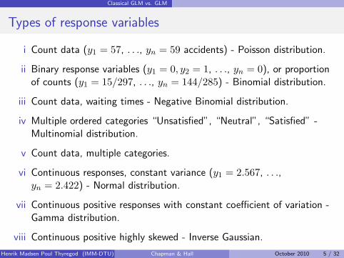
Types of response variables

i Count data (y1 = 57, . . ., yn = 59 accidents) - Poisson distribution.

ii Binary response variables (y1 = 0, y2 = 1, . . ., yn = 0), or proportionof counts (y1 = 15/297, . . ., yn = 144/285) - Binomial distribution.

iii Count data, waiting times - Negative Binomial distribution.

iv Multiple ordered categories “Unsatisfied”, “Neutral”, “Satisfied” -Multinomial distribution.

v Count data, multiple categories.

vi Continuous responses, constant variance (y1 = 2.567, . . .,yn = 2.422) - Normal distribution.

vii Continuous positive responses with constant coefficient of variation -Gamma distribution.

viii Continuous positive highly skewed - Inverse Gaussian.


Motivating example

Motivating example

The generalized linear model will be introduced in the following example.The generalized linear model will then be explained in detail in this andthe following lectures.

In toxicology it is usual practice to assess developmental effects of an agentby administering specified doses of the agent to pregnant mice, and assessthe proportion of stillborn as a function of the concentration of the agent.

The quantity of interest is the fraction, y, of stillborn pups as a function ofthe concentration x of the agent.

A natural distributional assumption is the binomial distribution

Y ∼ B(ni, pi)/ni

.


Motivating example

Motivating example

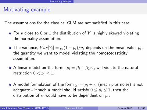
The assumptions for the classical GLM are not satisfied in this case:

For p close to 0 or 1 the distribution of Y is highly skewed violatingthe normality assumption.

The variance, V ar[Yi] = pi(1− pi)/ni depends on the mean value pi,the quantity we want to model violating the homoscedasticityassumption.

A linear model on the form: pi = βi + β2xi, will violate the naturalrestriction 0 < pi < 1.

A model formulation of the form yi = pi + εi (mean plus noise) is notadequate - if such a model should satisfy 0 ≤ yi ≤ 1, then thedistribution of εi would have to be dependent on pi.


Motivating example

Motivating example

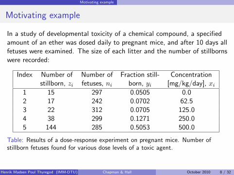
In a study of developmental toxicity of a chemical compound, a specifiedamount of an ether was dosed daily to pregnant mice, and after 10 days allfetuses were examined. The size of each litter and the number of stillbornswere recorded:

Index Number of Number of Fraction still- Concentrationstillborn, zi fetuses, ni born, yi [mg/kg/day], xi

1 15 297 0.0505 0.02 17 242 0.0702 62.53 22 312 0.0705 125.04 38 299 0.1271 250.05 144 285 0.5053 500.0

Table: Results of a dose-response experiment on pregnant mice. Number ofstillborn fetuses found for various dose levels of a toxic agent.


Motivating example

Motivating example

Let Zi denote the number of stillborns at dose concentration xi.

We shall assume Zi ∼ B(ni, pi), that is a binomial distributioncorresponding to ni independent trials (fetuses), and the probability, pi, ofstillbirth being the same for all ni fetuses.

We want to model Yi = Zi/ni, and in particular we want a model forE[Yi] = pi.


Motivating example

Motivating example

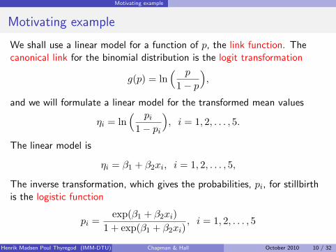
We shall use a linear model for a function of p, the link function. Thecanonical link for the binomial distribution is the logit transformation

g(p) = ln( p

1− p

),

and we will formulate a linear model for the transformed mean values

ηi = ln( pi

1− pi

), i = 1, 2, . . . , 5.

The linear model is

ηi = β1 + β2xi, i = 1, 2, . . . , 5,

The inverse transformation, which gives the probabilities, pi, for stillbirthis the logistic function

pi =exp(β1 + β2xi)

1 + exp(β1 + β2xi), i = 1, 2, . . . , 5


Motivating example

Motivating example - R

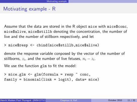
Assume that the data are stored in the R object mice with mice$conc,mice$alive, mice$stillb denoting the concentration, the number oflive and the number of stillborn respectively, and let

> mice$resp <- cbind(mice$stillb,mice$alive)

denote the response variable conposed by the vector of the number ofstillborns, zi, and the number of live fetuses, ni − zi.

We use the function glm to fit the model:

> mice.glm <- glm(formula = resp ~ conc,family = binomial(link = logit), data= mice)


Motivating example


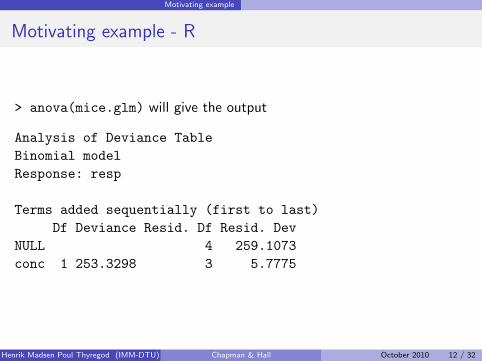
> anova(mice.glm) will give the output

Analysis of Deviance TableBinomial modelResponse: resp

Terms added sequentially (first to last)Df Deviance Resid. Df Resid. Dev

NULL 4 259.1073conc 1 253.3298 3 5.7775


Motivating example


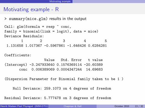
> summary(mice.glm) results in the output

Call: glm(formula = resp ~ conc,family = binomial(link = logit), data = mice)Deviance Residuals:

1 2 3 4 51.131658 1.017367 -0.5967861 -1.646426 0.6284281

Coefficients:Value Std. Error t value

(Intercept) -3.247933640 0.1576369114 -20.60389conc 0.006389069 0.0004347244 14.69683

(Dispersion Parameter for Binomial family taken to be 1 )

Null Deviance: 259.1073 on 4 degrees of freedom

Residual Deviance: 5.777478 on 3 degrees of freedom


Motivating example


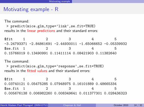
The command:> predict(mice.glm,type=’link’,se.fit=TRUE)

results in the linear predictions and their standard errors:

$fit 1 2 3 4 5-3.24793371 -2.84861691 -2.44930011 -1.65066652 -0.05339932$se.fit 1 2 3 4 50.15766019 0.13490991 0.11411114 0.08421903 0.11382640

The command:> predict(mice.glm,type=’response’,se.fit=TRUE)

results in the fitted values and their standard errors:

$fit 1 2 3 4 50.03740121 0.05475285 0.07948975 0.16101889 0.48665334$se.fit 1 2 3 4 50.005676138 0.006982260 0.008349641 0.011377301 0.028436323


Motivating example


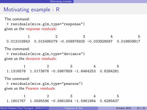
The command:> residuals(mice.glm,type="response")

gives us the response residuals:

1 2 3 4 50.013103843 0.015495079 -0.008976925 -0.033928587 0.018609817

The command:> residuals(mice.glm,type="deviance")

gives us the deviance residuals:

1 2 3 4 51.1316578 1.0173676 -0.5967859 -1.6464253 0.6284281

The command:> residuals(mice.glm,type="pearson")

gives us the Pearson residuals:

1 2 3 4 51.1901767 1.0595596 -0.5861854 -1.5961984 0.6285637


Motivating example

Motivating example

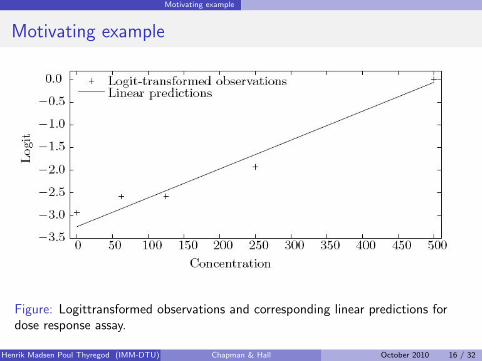
Figure: Logittransformed observations and corresponding linear predictions fordose response assay.


Motivating example

Motivating example

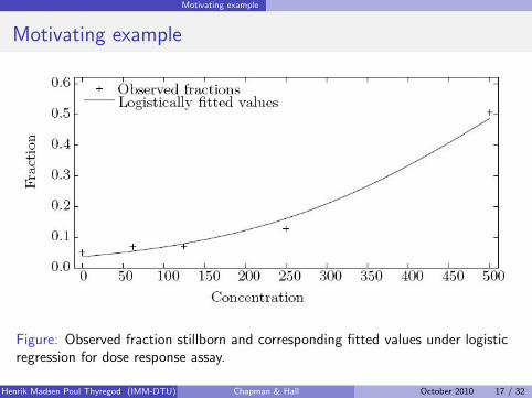
Figure: Observed fraction stillborn and corresponding fitted values under logisticregression for dose response assay.




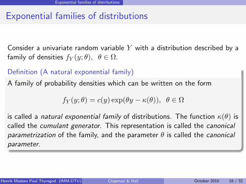
Consider a univariate random variable Y with a distribution described by afamily of densities fY (y; θ), θ ∈ Ω.

Definition (A natural exponential family)

A family of probability densities which can be written on the form

fY (y; θ) = c(y) exp(θy − κ(θ)), θ ∈ Ω

is called a natural exponential family of distributions. The function κ(θ) iscalled the cumulant generator. This representation is called the canonicalparametrization of the family, and the parameter θ is called the canonicalparameter.




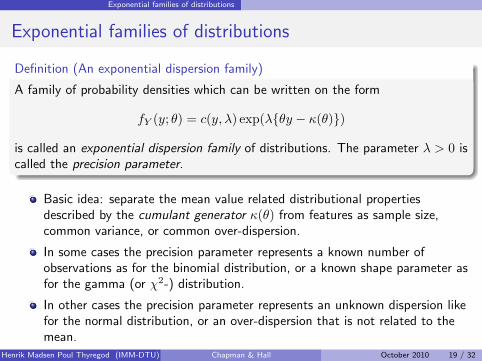
Definition (An exponential dispersion family)

A family of probability densities which can be written on the form

fY (y; θ) = c(y, λ) exp(λθy − κ(θ))

is called an exponential dispersion family of distributions. The parameter λ > 0 iscalled the precision parameter.

Basic idea: separate the mean value related distributional propertiesdescribed by the cumulant generator κ(θ) from features as sample size,common variance, or common over-dispersion.

In some cases the precision parameter represents a known number ofobservations as for the binomial distribution, or a known shape parameter asfor the gamma (or χ2-) distribution.

In other cases the precision parameter represents an unknown dispersion likefor the normal distribution, or an over-dispersion that is not related to themean.



Example: Poisson distribution

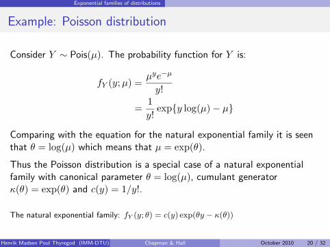
Consider Y ∼ Pois(µ). The probability function for Y is:

fY (y;µ) =µye−µ

y!

=1y!

expy log(µ)− µ

Comparing with the equation for the natural exponential family it is seenthat θ = log(µ) which means that µ = exp(θ).

Thus the Poisson distribution is a special case of a natural exponentialfamily with canonical parameter θ = log(µ), cumulant generatorκ(θ) = exp(θ) and c(y) = 1/y!.

The natural exponential family: fY (y; θ) = c(y) exp(θy − κ(θ))



Example: Normal distribution

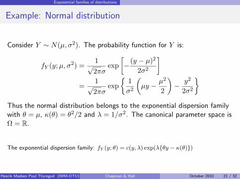
Consider Y ∼ N(µ, σ2). The probability function for Y is:

fY (y;µ, σ2) =1√2πσ

exp[−(y − µ)2

2σ2

]=

1√2πσ

exp

1σ2

(µy − µ2

2

)− y2

2σ2

Thus the normal distribution belongs to the exponential dispersion familywith θ = µ, κ(θ) = θ2/2 and λ = 1/σ2. The canonical parameter space isΩ = R.

The exponential dispersion family: fY (y; θ) = c(y, λ) exp(λθy − κ(θ))



Example: Binomial distribution

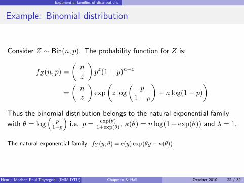
Consider Z ∼ Bin(n, p). The probability function for Z is:

fZ(n, p) =(nz

)pz(1− p)n−z

=(nz

)exp

(z log

(p

1− p

)+ n log(1− p)

)Thus the binomial distribution belongs to the natural exponential family

with θ = log(

p1−p

)i.e. p = exp(θ)

1+exp(θ) , κ(θ) = n log(1 + exp(θ)) and λ = 1.

The natural exponential family: fY (y; θ) = c(y) exp(θy − κ(θ))



Example: Binomial distribution

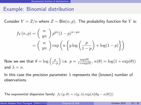
Consider Y = Z/n where Z ∼ Bin(n, p). The probability function for Y is:

fY (n, p) =(

nyn

)pyn(1− p)n−yn

=(

nyn

)exp

(n

y log

(p

1− p

)+ log(1− p)

)

Now we see that θ = log(

p1−p

)i.e. p = exp(θ)

1+exp(θ) , κ(θ) = log(1 + exp(θ))and λ = n.

In this case the precision parameter λ represents the (known) number ofobservations.

The exponential dispersion family: fY (y; θ) = c(y, λ) exp(λθy − κ(θ))



Mean and variance

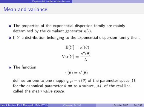
The properties of the exponential dispersion family are mainlydetermined by the cumulant generator κ(·).

If Y a distribution belonging to the exponential dispersion family then:

E[Y ] = κ′(θ)

Var[Y ] =κ′′(θ)λ

The functionτ(θ) = κ′(θ)

defines an one to one mapping µ = τ(θ) of the parameter space, Ω,for the canonical parameter θ on to a subset, M, of the real line,called the mean value space.



(Unit) variance function

(Unit) variance function

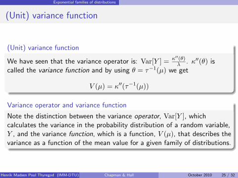
We have seen that the variance operator is: Var[Y ] = κ′′(θ)λ . κ′′(θ) is

called the variance function and by using θ = τ−1(µ) we get

V (µ) = κ′′(τ−1(µ))

Variance operator and variance function

Note the distinction between the variance operator, Var[Y ], whichcalculates the variance in the probability distribution of a random variable,Y , and the variance function, which is a function, V (µ), that describes thevariance as a function of the mean value for a given family of distributions.



The deviance

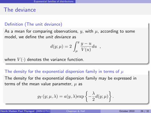
Definition (The unit deviance)

As a mean for comparing observations, y, with µ, according to somemodel, we define the unit deviance as

d(y;µ) = 2∫ y

µ

y − uV (u)

du ,

where V (·) denotes the variance function.

The density for the exponential dispersion family in terms of µ

The density for the exponential dispersion family may be expressed interms of the mean value parameter, µ as

gY (y;µ, λ) = a(y, λ)exp−λ

2d(y;µ)

.



Alternative definition of the deviance

Alternative definition of the deviance

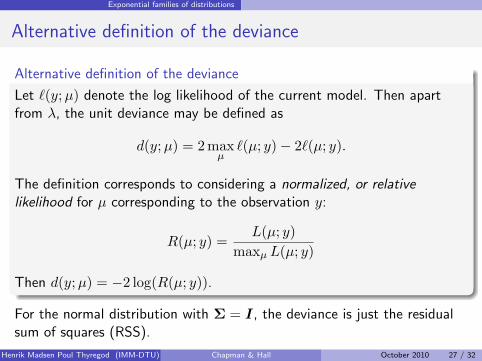
Let `(y;µ) denote the log likelihood of the current model. Then apartfrom λ, the unit deviance may be defined as

d(y;µ) = 2 maxµ

`(µ; y)− 2`(µ; y).

The definition corresponds to considering a normalized, or relativelikelihood for µ corresponding to the observation y:

R(µ; y) =L(µ; y)

maxµ L(µ; y)

Then d(y;µ) = −2 log(R(µ; y)).

For the normal distribution with Σ = I, the deviance is just the residualsum of squares (RSS).



Variance function, unit deviance and λ

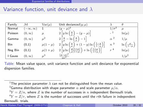
Family M Var(µ) Unit devianced(y;µ) λ θNormal (−∞,∞) 1 (y − µ)2 1/σ2 µ

Poisson (0,∞) µ 2hy ln

“yµ

”− (y − µ)

i- 1 ln(µ)

Gamma (0,∞) µ2 2hyµ− ln

“yµ

”− 1i

α 2 1/µ

Bin (0,1) µ(1− µ) 2hy ln

“yµ

”+ (1− y) ln

“1−y1−µ

”in 3 ln

“µ

1−µ

”Neg Bin (0,1) µ(1 + µ) 2

hy ln

“y(1+µ)µ(1+y)

”+ ln

“1+µ1+y

”ir 4 ln(µ)

I Gauss (0,∞) µ3 (y−µ)2

yµ2 1/µ2

Table: Mean value space, unit variance function and unit deviance for exponentialdispersion families.

1The precision parameter λ can not be distinguished from the mean value.2Gamma distribution with shape parameter α and scale parameter µ/α.3Y = Z/n, where Z is the number of successes in n independent Bernoulli trials.4Y = Z/r, where Z is the number of successes until the rth failure in independent

Bernoulli. trials.Henrik Madsen Poul Thyregod (IMM-DTU) Chapman & Hall October 2010 28 / 32


Exponential dispersion family

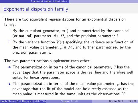
There are two equivalent representations for an exponential dispersionfamily:

i By the cumulant generator, κ(·) and parametrized by the canonical(or natural) parameter, θ ∈ Ω, and the precision parameter λ

ii By the variance function V (·) specifying the variance as a function ofthe mean value parameter, µ ∈M, and further parametrized by theprecision parameter λ.

The two parametrizations supplement each other:

The parametrization in terms of the canonical parameter, θ has theadvantage that the parameter space is the real line and therefore wellsuited for linear operations,

The parametrization in terms of the mean value parameter, µ has theadvantage that the fit of the model can be directly assessed as themean value is measured in the same units as the observations, Y .



Exponential family densities as a statistical model

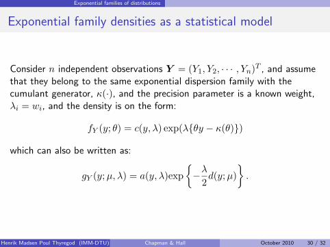
Consider n independent observations Y = (Y1, Y2, · · · , Yn)T , and assumethat they belong to the same exponential dispersion family with thecumulant generator, κ(·), and the precision parameter is a known weight,λi = wi, and the density is on the form:

fY (y; θ) = c(y, λ) exp(λθy − κ(θ))

which can also be written as:

gY (y;µ, λ) = a(y, λ)exp−λ

2d(y;µ)

.



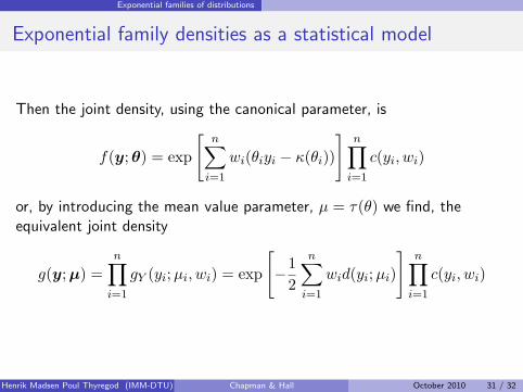
Exponential family densities as a statistical model

Then the joint density, using the canonical parameter, is

f(y;θ) = exp

[n∑i=1

wi(θiyi − κ(θi))

]n∏i=1

c(yi, wi)

or, by introducing the mean value parameter, µ = τ(θ) we find, theequivalent joint density

g(y;µ) =n∏i=1

gY (yi;µi, wi) = exp

[−1

2

n∑i=1

wid(yi;µi)

]n∏i=1

c(yi, wi)



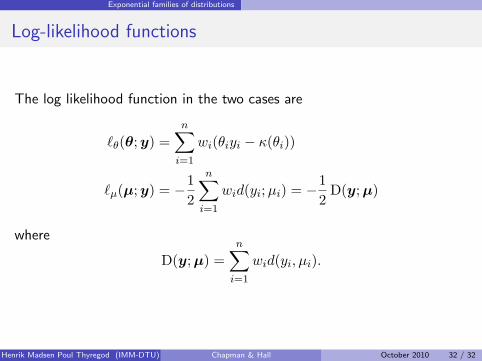
Log-likelihood functions

The log likelihood function in the two cases are

`θ(θ;y) =n∑i=1

wi(θiyi − κ(θi))

`µ(µ;y) = −12

n∑i=1

wid(yi;µi) = −12

D(y;µ)

where

D(y;µ) =n∑i=1

wid(yi, µi).


Introduction to General and Generalized Linear Models ...hmad/GLM/slides/lect06.pdf · Introduction...

Documents

Transcript of Introduction to General and Generalized Linear Models ...hmad/GLM/slides/lect06.pdf · Introduction...