Generality’s price: Inescapable deficiencies in machine-learned programs

Annals of Pure and Applied Logic 139 (2006) 303–326

www.elsevier.com/locate/apal

Generality’s price: Inescapable deficiencies inmachine-learned programs

John Casea, Keh-Jiann Chenb, Sanjay Jainc, Wolfgang Merkled,James S. Royere,∗

aDepartment of Computer and Information Sciences, University of Delaware, Newark, DE 19716-2586, USAbInstitute of Information Science, Academia Sinica, Nankang 115, Taipei, Taiwan, ROC

cSchool of Computing, National University of Singapore, 3 Science Drive 2, Singapore 117543,Republic of Singapore

dUniversität Heidelberg, Mathematisches Institut, Im Neuenheimer Feld 294, D-69120 Heidelberg, GermanyeDepartment of Electrical Engineering and Computer Science, Syracuse University, Syracuse, NY 13244, USA

Received 6 January 2005; received in revised form 23 May 2005; accepted 7 June 2005Available online 19 July 2005

Communicated by R.I. Soare

Abstract

This paper investigates some delicate tradeoffs between thegeneralityof an algorithmic learningdevice and thequality of the programs it learns successfully. There are results to the effect that,thanks to small increases in generality of a learning device, the computational complexity ofsome successfully learned programs is provably unalterablysuboptimal. There are also results inwhich the complexity of successfully learned programsis asymptotically optimal and the learningdevice is general, but, still thanks to the generality, some of those optimal, learned programsare provably unalterablyinformation deficient—in some cases, deficient as to safe, algorithmicextractability/provability of the fact that they are even approximately optimal. For these results, thesafe, algorithmic methods of information extraction will be by proofs in arbitrary, true, computablyaxiomatizable extensions of Peano Arithmetic.© 2005 Elsevier B.V. All rights reserved.

∗ Corresponding author.E-mail addresses:[email protected] (J. Case), [email protected] (K.-J. Chen),

[email protected] (S. Jain), [email protected] (W. Merkle), [email protected](J.S. Royer).

0168-0072/$ - see front matter © 2005 Elsevier B.V. All rights reserved.doi:10.1016/j.apal.2005.06.013

http://www.elsevier.com/locate/apal

304 J. Case et al. / Annals of Pure and Applied Logic 139 (2006) 303–326

Keywords:Computational learning theory; Applications of computability theory

1. Introduction

We abbreviateclass of characteristic functions of languagesas CCFL. SupposeC0 ⊆ C1is a pair of complexity CCFLs whichdo (perhaps barely) separate. For example, letα,as from [9, Section 21.4], be avery slow growing, linear time computable function≤an inverse of Ackermann’s function; letC1 be DTIME(n · (logn) · α(n)); and letC0 beDTIME(n).1 These classes have long been known to separate [13,15]. Furthermore, itis straightforward to see thatsomelearning device (synonymously, inductive inferencemachine or IIM)M0, fed the values of any elementf of thisC0, outputs nothing but linear-time programs and eventually converges to a fixed linear-time program which correctlycomputes f . This kind of syntactically converging learning in the limit is called EX-learning (or EX-identification) [12,4,6,16]. Let Z∗ be the CCFL for precisely thefinitelanguages. Clearly,Z∗ is an especially simple, proper subclass of our exampleC0. Two ofour main theorems (Theorems 27and28 in Section 6below) each imply that, nonetheless,if M1 is any learning device which is slightly more general thanM0 in that it EX-learnsevery function in our exampleC1, then, for some especially “easy” functionf , moreparticularly for an f ∈ Z∗, M1 on f syntactically converges to a correct programp forf , but this p runs in worse than any linear-time boundon all but finitely many inputs. Thisinherentrun-time deficiency ofp is the inescapableprice for employing a more generallearning device to learnC1 instead of learning onlyC0. Theorems 27and28, on which thisexample is based, are proved by delayed diagonalization (or slowed simulation) [20,30]with cancellation [3] (or zero injury), complexity-bounded self-reference [30], and carefulsubrecursive programming [30].

Fix k ≥ 1. Let C1 = DTIME(nk · (logn) · α(n)) and C0 = DTIME(nk). Theseclasses separate [13,15], and it is straightforward that some learning device EX-learnsthis C0 outputting only conjectures that run ink-degree polytime. However, again fromTheorems 27and28, for any slightly more general learning deviceM1 which EX-learnsthis C1, there will be an easyf , an f ∈ Z∗, so that, onf , M1’s final programp will runworse than anyk-degree polytime bound on all but finitely many inputs.

One way to circumvent the complexity-deficiency-in-learned-programs price of gener-ality in the above examples is to consider a most general learning criterion called BC∗-learning [6,5]. In this type of learning, in contrast to EX-learning, one foregoes syntacticconvergence in favor of semantic convergence and one foregoes requiring the final pro-grams to be perfectly correct at computing the input function: convergence is to an infinitesequence of programs all but finitely many of which are each correct on all but finitelymany inputs. Harrington [6] showed that there is a learning device that BC∗-learnseverycomputable function. (On the other hand, fairly simple classes of computable functions

1 DTIME(t (n)) denotes the set oflanguagesdecidable by a deterministic, multi-tape Turing machine withinO(t (n)) time, wheren is the length of the machine’s input. DTimeF(t (n)) denotes the set offunctionsover stringscomputable by this same class of machines withinO(t (n)) time.

J. Case et al. / Annals of Pure and Applied Logic 139 (2006) 303–326 305

cannot be EX-learned [6].) One of our main positive results (Theorem 31in Section 8below) says that there is a learning deviceM∗ that BC∗-learns the CCFL for the polytimedecidable languages in such a way that: (i) all ofM∗’s output conjectures run in polytime;(ii) for eachk ≥ 1, on eachf ∈ DTIME(nk), all but finitely many ofM∗’s outputs run ink-degree polytime;and(iii) M∗ EX-learns all the linear-time computable functions.

There is, though, another kind of deficiency-in-learned-programs price for generalityof learning, and this affects BC∗-learning, EX-learning, and the learning criteria ofintermediate strength discussed, beginning inSection 2, below. LetPFk = DTimeF(nk)

andQFkα = DTimeF(nk · (logn) · α(n)). Let ϕq be the (partial) function computed by

multi-tape Turing machine (number)q. SupposeM is any device BC∗-learningQFkα .2

Corollary 9in Section 4below says, then, that there is an easyf , an f ∈ Z∗, such that, ifM is fed the values off (which it at least BC∗-learns), then for all but finitely many ofM’scorresponding output conjecturesp, Peano Arithmetic [25] (PA) fails to prove that somefinite variant ofϕp is k-degree polytime computable. Of course, for suchp’s, some finitevariant ofϕp, e.g., f , is trivially linear-timecomputable. Hence, thesep’s areinformation-deficient. If, for example,M∗, the learning device ofTheorem 31(discussed in the previousparagraph), is used forM, then, on the correspondingf , thisM outputs aperfectly correctfinal programp which runs in linear time, but Peano Arithmetic cannot prove the weakerresult about thisp that some finite variant ofϕp is k-degree polytime computable. Hence,for the learning device ofTheorem 31, its final output onf is information-deficient, butnotcomplexity-deficient.Corollary 9discussed in this paragraph is one of several corollariesof Theorem 8, our first main sufficient condition result, all given inSection 4.

Here is another example. LetC0 = REG andC1 = CF , whereREG andCF are theCCFLs of regular and context free languages, respectively. Of course, for this example,the separation is not particularly tight. However, importantly, for this example, direct,aggressive diagonalization methods such as those mentioned above are not available. LetcoZ∗ be the CCFL for theco-finite languages, i.e., the languages whose complementsare finite. Clearly,coZ∗ is an especially simple, proper subclass ofREG. First note thatsome learning device outputs only deterministic finite automata and EX-learnsREG [12],where deterministic finite automata should be thought of as a degenerate case of Turingmachines that useno tape squares for workspace [15]. EX∗-learning is the variant of EX-learning in which the final program need be correct only on all but finitely many inputs. Bycontrast, still inSection 4below, as a corollary of our other main sufficient condition result,Theorem 14, we haveCorollary 17as follows. SupposeM EX∗-learnsCF andk,n ≥ 1.3

Then there is an easyf , an f ∈ coZ∗, such that, ifp is M’s final program onf , forsome distinct x0, . . . , xn−1, programp uses more thank workspace squares on each ofinputsx0, . . . , xn−1. This is a complexity-deficiency result for(REG, CF). Theorem 14has other complexity-deficiency corollaries, e.g.,Corollary 18, an interesting one for(P,NP)—assumingthey separate. See alsoRemark 20for a related interesting corollaryinvolving BQP, a quantum version of polynomial-time [2], instead of NP. In these resultsthe complexity-deficient learned programs haveunnecessary non-determinism or quantum

2 One of many special cases of this hypothesis is thatM actually EX-learnsQFkα .

3 One of many special cases of the hypothesis thatM EX∗-learnsCF is thatM actually EX-learnsCF .


parallelism.Corollaries 10and 11 of Theorem 8provide information-deficiency resultsfor (REG, CF) and (P,NP), respectively.Remark 12provides information-deficiencycorollaries ofTheorem 8for (P,BQP) as well as other examples.

Those corollaries, discussed in the previous paragraph, of our sufficient conditionresults, Theorems 8and 14, involve classes(C0, C1) for which direct, aggressivediagonalization is (apparently) not available. These sufficient condition results are provedherein with the aid of some refinedinseparability results from [30]. Section 3belowprovides the details. In [30] the inseparabilities were used to characterize relative programsuccinctness between (possibly barely) separated subrecursive programming systems.Herein they are used to obtain higher-type inseparabilities providing our sufficientconditions (not characterizations) for deficiencies in machine-learned programs. We alsouse Theorem 8to obtain all ourinformation-deficiencyresults, including the one for(PFk,QFk

α) described above. Actually,Theorem 14can be used to prove a weak specialcase of our strong complexity-deficiency result (Theorem 28) for (PFk,QFk

α). This isCorollary 16. In this corollary the quantifierorder between thef ∈ Z∗ and thek-degreepolynomial-time bounds is weakened and the for-all-but-finitely-many-inputs-x quantifieris weakened to exists-n-distinct-inputs.

Someof our results whose proofs employ tricks from [30] can also be shown throughrelated methods from [31,32,27], but we do not pursue this further here.

The order of presentation in this introduction differs from that of the remaining sections.The latter order was dictated, to some extent, by the need to introduce required technologyin a particular order.

2. Conventions and notation

Strings and numbers.N denotes the set of non-negative integers. Each element ofN isidentified with its dyadic representation over{ 0, 1 }. Thus, 0≡ ε, 1 ≡ 0, 2 ≡ 1, 3 ≡ 00,etc. We will freely pun betweenx ∈ N as a number and a0-1-string. Let|x| = the length ofthe dyadic representation ofx ∈ N. By convention, for x ∈ Nn, | x| = |x0| + · · · + |xn−1|.Encoding tuples.Let 〈·, ·〉 be a linear time pairing function. That is,〈·, ·〉 : N×N → N is1–1 and onto and each ofλx, y 〈x, y〉,π0 = λ〈x, y〉 x, andπ1 = λ〈x, y〉 y is computableon a multi-tape deterministic Turing Machine in time linear in the lengths of its inputs.Examples of such pairing functions can be found in [28,30]. By convention, for eachn ≥ 2andx0, . . . , xn ∈ N, we inductively define〈x0, . . . , xn〉 = 〈x0, 〈x1, . . . , xn〉〉.Functions. A→ B (respectively,A ⇀ B) denotes the set of all total (respectively,possibly partial) functions fromA to B. For f : A ⇀ B, f (x)↓ means f is defined onx and f (x)↑ means thatf (x) is undefined onx; ↑ by itself denotesundefined. Supposef, g : N ⇀ N. For eachn ∈ N, f =n g means that{ x f (x) �= g(x) } is of sizen or less,and f =∗ g means that{ x f (x) �= g(x) } is finite, i.e., thatf andg arefinite variants.For eachf : N → N, let

O( f )def= { g : N → N (∃a)(∀x)[ g(x) ≤ a · ( f (x)+ 1) ] }.

By conventionO( f (n)) is short for O(λx f (|x|)). For eachC ⊆ (N → N), let C0-1denote the 0–1 valued elements ofC. PR denotes the set of partial recursive functions and


R denotes the total recursive functions. Let log 0= 0 and, for each positive integerx,logx = �log2 x�.Programming systems.A partial recursiveψ : N2 ⇀ N is a programming systemforS ⊆ PR if and only if S = { λx ψ(i , x) i ∈ N }. We typically writeψi (x) forψ(i , x). Letϕ be an acceptable programming system ofPR based on deterministic multi-tape Turing machines [15,17]; ϕ beingacceptablemeans that for any other programmingsystem for anS ⊆ PR, sayθ , there is an effective translation ofθ -programs into equivalentϕ-programs, i.e., a computablet with ϕt (i ) = θi for all i . By convention, for eachi andx, x0, . . . , xk, ϕi (x0, . . . , xk) = ϕi (〈x0, . . . , xk〉); Φi (x) = the run time of TMi on inputx; andΦWS

i (x) = the work space used by TMi on inputx, providedϕi (x)↓;∞, otherwise.

Subrecursive classes of functions.For each recursivet : N → N, let DTimeF(t) = { ϕi

(∃a)(∀x)[Φi (x) ≤ a · (t (x)+ 1) ] } and DTIME(t) = (DTimeF(t))0-1. For eachk > 0, let

PFk def= DTimeF(λx |x|k),the functions computable inO(nk) time on a deterministic multi-tape TM, and letPF =∪k>0PFk, the polynomial-time computable functions. Let

LS lowdef=

{f ∈ PF1 f is nondecreasing and unbounded

}.

By standard results [8,21], for each recursive, increasing, unboundedf , there is ans ∈ LS low that grows slower than the inverse off in the sense thats( f (x)) ≤ x forall x. For eachk > 0 ands ∈ LS low,

QFks

def= DTimeF(λx |x|k · (log |x|) · s(|x|)

).

By standard results [13,15], (QFks − PFk)0-1 �= ∅ for eachk > 0 ands ∈ LS low.

Let Z∗ (respectively,coZ∗) denote the class of 0–1 valued functions that are 0(respectively, 1) almost everywhere. LetNP , BPP, P , CF , andREG respectively denotethe classes of characteristic functions of NP, BPP [11], polynomial-time decidable, contextfree, and regular languages over{ 0, 1 }∗. (Recall:N ≡ { 0, 1 }∗.)

S ⊆ R is an r.e. subrecursive classwhen there is a programming system forS. Bystandard results,P , Pk, QFk

s, NP , . . . are each r.e. subrecursive classes.

Finite initial segments.For f : N → N andn ∈ N, f |n denotes the sequencef (0), f (1),. . . , f (n − 1), the length-n initial segment of f . So, f |0 = the empty segment. LetSEG= the set of all such finite initial segments;σ , with or without decorations, rangesover SEG. Ifσ = a0,a1, . . . ,an−1 andm ≤ n, thenσ |m = a0,a1, . . . ,am−1.

Inductive inference machines.An inductive inference machine[12] is an algorithmicdevice that computes a SEG⇀ N function.M, with or without decorations, ranges oversuch machines. Since SEG can be coded intoN, an M can be viewed as computing anelement ofPR. M on f convergesto i (written: M( f )↓ = i ) when, for all but finitelymanyn, M( f |n) = i ; M( f ) is undefined if no suchi exists. Thepoint of convergenceof Mon f is, if it exists, the smallestm with M( f |m)↓ andM( f |n) = M( f |m) for eachn > m.


✣✢✤✜

A ✣✢✤✜

B

S

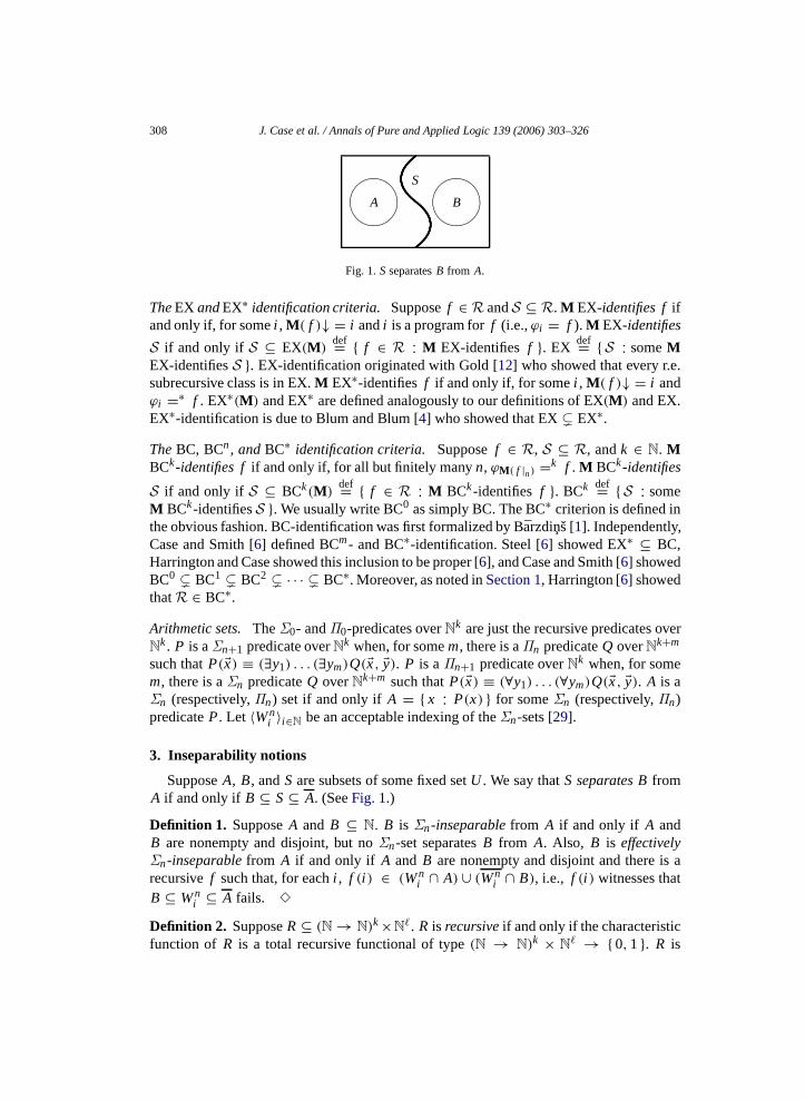
Fig. 1. SseparatesB from A.

TheEX andEX∗ identification criteria. Supposef ∈ R andS ⊆ R. M EX-identifies f ifand only if, for somei , M( f )↓ = i andi is a program forf (i.e.,ϕi = f ). M EX-identifies

S if and only if S ⊆ EX(M) def= { f ∈ R M EX-identifies f }. EXdef= {S someM

EX-identifiesS }. EX-identification originated with Gold [12] who showed that every r.e.subrecursive class is in EX.M EX∗-identifies f if and only if, for somei , M( f )↓ = i andϕi =∗ f . EX∗(M) and EX∗ are defined analogously to our definitions of EX(M) and EX.EX∗-identification is due to Blum and Blum [4] who showed that EX� EX∗.

TheBC, BCn, andBC∗ identification criteria. Supposef ∈ R, S ⊆ R, andk ∈ N. MBCk-identifies f if and only if, for all but finitely manyn, ϕM( f |n) =k f . M BCk-identifies

S if and only if S ⊆ BCk(M)def= { f ∈ R M BCk-identifies f }. BCk def= {S some

M BCk-identifiesS }. We usually write BC0 as simply BC. The BC∗ criterion is defined inthe obvious fashion. BC-identification was first formalized by Barzdinš [1]. Independently,Case and Smith [6] defined BCm- and BC∗-identification. Steel [6] showed EX∗ ⊆ BC,Harrington and Case showed this inclusion to be proper [6], and Case and Smith [6] showedBC0 � BC1 � BC2 � · · · � BC∗. Moreover, as noted inSection 1, Harrington [6] showedthatR ∈ BC∗.

Arithmetic sets. TheΣ0- andΠ0-predicates overNk are just the recursive predicates overNk. P is aΣn+1 predicate overNk when, for somem, there is aΠn predicateQ overNk+m

such thatP( x) ≡ (∃y1) . . . (∃ym)Q( x, y). P is aΠn+1 predicate overNk when, for somem, there is aΣn predicateQ overNk+m such thatP( x) ≡ (∀y1) . . . (∀ym)Q( x, y). A is aΣn (respectively,Πn) set if and only ifA = { x P(x) } for someΣn (respectively,Πn)predicateP. Let 〈Wn

i 〉i∈N be an acceptable indexing of theΣn-sets [29].

3. Inseparability notions

SupposeA, B, andS are subsets of some fixed setU . We say thatS separates BfromA if and only if B ⊆ S⊆ A. (SeeFig. 1.)

Definition 1. SupposeA and B ⊆ N. B is Σn-inseparablefrom A if and only if A andB are nonempty and disjoint, but noΣn-set separatesB from A. Also, B is effectivelyΣn-inseparablefrom A if and only if A and B are nonempty and disjoint and there is arecursivef such that, for eachi , f (i ) ∈ (Wn

i ∩ A) ∪ (Wni ∩ B), i.e., f (i ) witnesses that

B ⊆ Wni ⊆ A fails. ✸

Definition 2. SupposeR⊆ (N → N)k×N�. R is recursiveif and only if the characteristicfunction of R is a total recursive functional of type(N → N)k × N� → { 0,1 }. R is


arithmeticalif and only if eitherR is recursive or

R ={( f , x) (Q1 y1) . . . (Qm ym)[ S( f , x, y) ]

}(1)

where eachQi is either∃ or∀ and whereS⊆ (N → N)k×N�+m is recursive. (N.B. All thequantifiers in (1) are numeric.)R is in Σ (fn)

n if and only if R is recursive orR is expressibleas in (1) with the quantifiers inΣn form. R is in Π (fn)

n if and only if R’s complement is inΣ (fn)

n . ✸

Indexings.For eachk, �, andn, let 〈W(fn),k,�,ni 〉i∈N be an acceptable indexing of the class of

all R⊆ (N → N)k×N� in Σ (fn)n (see [29, Section 15.2]). For eachi , letWn

i = W(fn),1,0,ni .

Next we introduce the higher-type inseparabilities needed for our results.

Definition 3. SupposeA andB ⊆ (N → N). B is Σ (fn)n -inseparablefrom A if and only

if A andB are nonempty and disjoint, but noΣ (fn)n -set separatesB from A. Also, B is

effectivelyΣ (fn)n -inseparablefromA if and only ifA andB are nonempty and disjoint and

there is a recursivef such that for eachi , ϕ f (i ) ∈ (Wni ∩A) ∪ (Wn

i ∩ B). ✸

The next proposition gives us a way of establishing aΣ (fn)2 -inseparability through the

Σ2-inseparability of certain sets of programs.

Proposition 4. Suppose the following:

(i) C is a subrecursive class with programming systemψ.(ii) A andB are disjoint and bothA ∩ C andB ∩ C are nonempty.(iii) { i ψi ∈ B } is effectivelyΣ2-inseparable from{ i ψi ∈ A }.ThenB is effectivelyΣ (fn)

2 -inseparable fromA.

Proof. Supposer witnesses the effectiveΣ2-inseparability of{ i ψi ∈ B } from{ i ψi ∈ A }. By standard results (see [29, Section 15.2]), there is a recursiveR ⊆ (N → N) × N3 such that, for all j , W2

j = { f (∃m)(∀n)R( f,m,n, j ) }.By a few more standard results, there is a recursive functiong such that, for all j ,W2

g( j ) = { i (∃m)(∀n)R(ψi ,m,n, j ) } = { i ψi ∈ W2j }. Let t be a recursive function

such thatϕt (i ) = ψi for all i . It follows thatr ′ = t ◦ r ◦ g is recursive and witnesses the

effectiveΣ (fn)2 -inseparability ofB fromA. �

The next proposition provides an alternative, often handier, way of showingΣ (fn)2 -

inseparability. Note, however, that the proof of this proposition depends onProposition 4.Recall:PF1 = the linear-time computable functions and(C)0-1 = the 0–1 valued elementsof C.

Proposition 5. Suppose thatC0, C1 ⊆ (N → N) are such that:

(i) BothC0 andC1 are closed under 0–1 valued finite variants.(ii) PF1 ⊆ C0 ∩ C1.(iii) For each f ∈ PF1 and g,h ∈ C1, f ◦ g, g◦ f , andλx 〈g(x),h(x)〉 ∈ C1.


(iv) There is a programming system forC1.(v) (C1− C0)0-1 �= ∅.

Then,(C1 − C0)0-1 is effectivelyΣ (fn)2 -inseparable fromZ∗.

There are many ways to establish this proposition using results from the structuralcomplexity literature, for example [32,31,27,30]. The proof given below uses a tool from[30], restated as the following lemma. Theϕ∗ of condition f is an acceptable programmingsystem for the partial recursive functions relative to an oracle for the halting problem[29,30]. Notation:For eachf, g,h : N ⇀ N, defineCond: (N ⇀ N)3 → (N ⇀ N) by

Cond( f, g,h)(x) =

g(x), if f (x) > 0;

h(x), if f (x) = 0;;

↑, if f (x)↑.(2)

Lemma 6 ([30, Theorem 9.11]). Suppose thatC0, andC1 are subrecursive classes,A ⊆(C0∩C1)0-1, D ⊆ C1, and there is a programming systemψ for C1. Moreover, suppose thatthe following conditions hold:

a. There is a g1 ∈ (C1)0-1 with { f : N → { 0,1 } f =∗ g1 } ⊆ (C1 − C0).b. There is a g0 ∈ A with { f : N → { 0,1 } f =∗ g0 } ⊆ A.c. For each f ∈ D and g,h ∈ C1, Cond( f, g,h) ∈ C1.d. For each f ∈ C1, f ◦ π0, f ◦ π1 ∈ C1.e. For each m and n > 0, there is a computable function s such that, for all

i , x1, . . . , xm, y1, . . . , yn, ψs(i, x)(〈 y 〉) = ψi (〈 x, y 〉).f. There is an L∈ D such that, for all i and x,limt→∞ L(〈i , x, t〉) = ϕ∗i (x), where

ϕ∗i (x)↓ = y ⇐⇒ (∞∀ t)[L(〈i , x, t〉) = y].

Then{ i ψi ∈ (C1 − C0)0-1 } is effectivelyΣ2-inseparable from{ i ψi ∈ A }.Proof (of Proposition 5). Let A = Z∗ andD = PF1. By (ii), (iv), and general resultson programming systems in [30, Section 4.2], we may assume thatψ is a programmingsystem forC1 that satisfies condition e. We note thatC0, C1, A, D, andψ together satisfythe hypotheses of the lemma. Specifically: conditions a and b follow from (i) and (v),conditions c and d follow from (ii) and (iii), condition e follows from our choice ofψ, and condition f follows from (ii) and Theorem 7.4 of [30]. Hence by the lemma,{ i ψi ∈ (C1 − C0)0-1 } is effectivelyΣ2-inseparable from{ i ψi ∈ A }. Therefore,by Proposition 4we have that(C1 − C0)0-1 is effectivelyΣ (fn)

2 -inseparable fromZ∗. �

Now, usingPropositions 4and 5 and few other results from the literature, we canestablish some sampleΣ (fn)

2 -inseparability results for some of the subrecursive classesintroduced inSection 2.

Corollary 7. Suppose k> 0 and s∈ LS low.

(a) (QFks − PFk)0-1 is effectivelyΣ (fn)

2 -inseparable fromZ∗.(b) (CF −REG) is effectivelyΣ (fn)

2 -inseparable from coZ∗.


(c) If P �= NP, then(NP − P) is effectivelyΣ (fn)2 -inseparable fromZ∗.

(d) If P �= BPP, then(BPP − P) is effectivelyΣ (fn)2 -inseparable fromZ∗.

Proof. Part (a). As previously noted,(QFks)0-1 and(PFk)0-1 separate by classic results

[13,15]. It is then straightforward that hypotheses (i) through (v) ofProposition 5aresatisfied. Thus, part (a) follows from the proposition.

Part (b). By the proof of Corollary 11.17 of [30], there is a programming systemψfor CF such that{ i ψi ∈ (CF −REG) } is effectivelyΣ2-inseparable from{ i ψi ∈coZ∗ }. Thus, part (b) follows byProposition 4.

Part (c). SupposeC1 = NP andC0 = P . Then it is straightforward that (i) through (iv)of Proposition 5are satisfied. The P�= NP hypothesis implies (v). Thus, part (c) followsfrom the proposition.

Part (d). This follows from an argument similar to the one for part (c).�

4. Sufficient conditions theorems

In the following, think ofA as some set of very modest functions (e.g.,Z∗ above),Bas some set of immodest functions, andG as some set of “good” programs4 such that nofinite variant of a member ofB has a program inG.

Theorem 8, our first sufficient condition theorem, provides us with our informationdeficiency corollaries (Corollaries 9through11). Notation:FV(B) = { f : N → N f isa finite variant of some element ofB }.Theorem 8. Suppose that:

(i) B is Σ (fn)2 -inseparable fromA.

(ii) G is aΣ1-set withFV(B) ∩ { ϕi i ∈ G } = ∅.(iii) M is an IIM such thatB ⊆ BC∗(M).

Then there is an f∈ A such that for all but finitely many n,M( f |n) /∈ G.

Proof. SinceG is a Σ1-set, there is a recursive predicateRG such thatG = { x (∃m)

RG(x,m) }. ConsiderS = { f (∞∀n)[M( f |n) /∈ G ]} ={

f (∃n0)(∀n > n0)(∀m)[ ¬RG(M( f |n),m) ]}.

Thus,S ∈ Σ (fn)2 . Also, by (ii) and (iii) it follows thatB ⊆ S. Now suppose the negation of

the conclusion: that for allf ∈ A, (∞∃n)[M( f |n) ∈ G ]. Clearly,A ∩ S = ∅. Therefore,

not (i) sinceS is aΣ (fn)2 -set separatingB fromA. �

The next three corollaries involve provability and PA, Peano Arithmetic [25]. We write& for the provability relation and�& for ‘doesnot prove’. The following predicates areexpressible in PA (and herein we do not distinguish between expressions in PA and

4 For example, the members ofG may run efficiently and/or be easy to prove things about.


expressions in the metalanguage):

Pk(i ) ≡def (∃c)(∀x)[Φi (x) ≤ c · (|x| + 1)k ].P∗k (i ) ≡def (∃ j | ϕ j =∗ ϕi )[ Pk( j ) ].P∗(i ) ≡def (∃k)[ P∗k (i ) ].Sk(i ) ≡def (∀x)[ΦWS

i (x) ≤ k ].REG∗(i ) ≡def (∃k)(∃ j | ϕ j =∗ ϕi )[ Sk( j ) ].

N.B. Each ofCorollaries 9–11 remains true if PA is replaced by any true and computablyaxiomatized theory [25] extending the language of PA. Such theories, including PA itself,should be thought of as safe, algorithmic extractors of information: the safety is thatthey prove only true sentences; and, since they are computably axiomatized, there is anassociated automatic theorem prover, i.e., the set of theorems is r.e. [25].

Corollary 9. Suppose that k> 0, s ∈ LS low, andBC∗(M) ⊇ QFks. Then there is an

f ∈ Z∗ such that, for all but finitely many n,PA �& P∗k (M( f |n)).Proof. Let A = Z∗, B = (QFk

s − PFk), andG = {i PA & P∗k (i )

}. Now, applying

Corollary 7(a) andTheorem 8, we are done. �

Interpretation.Let M and f be as inCorollary 9.5 Then it must be the case that, forall but finitely manyn, the programM( f |n) computes a finite variant off , an almosteverywhere zero function. Of coursesomeprogram computesf in linear time. Yet, evenso, for sufficiently largen, the programsM( f |n) are so information deficient that PA failsto prove of them that they compute a finite variant of something (likef ) that hassomeprogram running ink-degree polynomial time. Analogous remarks apply to the next twocorollaries.

Corollary 10. SupposeBC∗(M) ⊇ CF . Then there is an f∈ coZ∗ such that, for all butfinitely many n,PA �& REG∗(M( f |n)).Proof. Let A = coZ∗, B = (CF − REG), andG = {

i PA & REG∗(i )}. Now, applying

Corollary 7(b) andTheorem 8, we are done. �

Corollary 11. SupposeBC∗(M) ⊇ NP and thatP �= NP. Then there is an f∈ Z∗ suchthat, for all but finitely many n,PA �& P∗(M( f |n)).Proof. Let A = Z∗, B = (NP − P), and G = {

i PA & P∗(i )}. Now, applying

Corollary 7(c) andTheorem 8, we are done. �

Remark 12. Corollaries 9–11provide only a small sample of the wide range of situationsto which Theorem 8applies. For example, one can replace NP inCorollary 11 withessentially any natural complexity class C containing P; then under the assumptions thatBC∗(M) ⊇ the class of characteristic functions of members of C and C�= P, one hasthe same conclusion asCorollary 11. So for C one can have BPP (bounded probabilistic

5 As noted inSection 1, an allowed special case is thatM actually EX-learnsQFkα .


polynomial-time [11]), BQP (a quantum version of polynomial-time [2]), PSPACE, andso on. The only work involved in showing these results is in establishing the analogue ofCorollary 7(c) for each of these classes, and this is straightforward using the results andtools of [30].6 ✸

Remark 13. We call the f asserted to exist inTheorem 8awitness to the deficiency. If wechange “Σ (fn)

2 -inseparable” to “effectivelyΣ (fn)2 -inseparable” inTheorem 8, then we can

strengthen that theorem’s conclusion to:there is a computable functionw such that, foreachi , if i is the index of an IIM satisfying hypothesis (iii), thenϕw(i ) ∈ A and, for allbut finitely manyn, M(ϕw(i )|n) /∈ G. So, thanks toCorollary 7, each ofCorollaries 9–11can have its conclusion correspondingly strengthened. In particular situations we can domuch better than this. For example, using the tools of [30] we can improve the conclusionof Corollary 9 to: There is a linear time computable functionw such that, for alli ,Φw(i ) ∈ O(nk · logn · s(n)) and, if i is the index of anM with BC∗(M) ⊇ QFk

s, thenϕw(i ) ∈ Z∗ and, for all but finitely manyn, PA �& P∗k (M(ϕw(i )|n)). ✸

Theorem 14, our second sufficient condition theorem, provides us with complexitydeficiency corollaries (Corollaries 16through19). Recall:FV(B) = { f (∃g ∈ B)[ f =∗g]}.Theorem 14. Suppose that:

(i) B is Σ (fn)2 -inseparable fromA.

(ii) G is aΠ2-set such thatFV(B) ∩ { ϕi i ∈ G } = ∅.(iii) M is an IIM such thatA ∪ B ⊆ EX∗(M).

Then there is an f∈ A such thatM( f ) /∈ G.

Proof. Since G is a Π2-set, there is a recursive predicateRG such thatG = { x(∀m)(∃n)RG(x,m,n) }. ConsiderS = { f M( f )↓ /∈ G] } ={

f (∃i ,m)(∀n0,n1 ≥ m)[

M( f |n0) = i & ¬RG(i ,m,n1)

] }.

Thus,S ∈ Σ (fn)2 . Also, by (ii) and (iii) it follows thatB ⊆ S. Now suppose the negation of

the conclusion: that for allf ∈ A, M( f )↓ ∈ G. Then clearly,A ∩ S = ∅. Therefore, not(i) sinceS is aΣ (fn)

2 -set separatingB fromA. �

Scholium 15. The fact thatG ∈ Π2 in Theorem 14fails to provide as much generalityas one might hope. Here is why. It is a well-worn observation that ifC is closed undertotal finite variants andP is a Σ2-set such thatC = { ϕi i ∈ P }, then there is anr.e. setP′ such thatC = { ϕi i ∈ P′ }. It is a minor variation on this observationthat if hypotheses (ii) and (iii) ofTheorem 14hold, then there is aΠ1-set G′ such that{ ϕi i ∈ G } ⊆ { ϕi i ∈ G′ } ⊆ (PR − FV(B)). Hence,G in Theorem 14might aswell beΠ1—which is what it is in our applications of this theorem.✸

6 BQP is not discussed in [30]. However, as BQP amounts to a quantum version of BPP, all the results neededto show the BQP analogue ofCorollary 7(c) can be obtained by a straightforward modification of the BPP resultsin [30]. Of course, then, [30, Corollary 11.10], a relative program succinctness result for, for example, BPP vs. P,also holds for BQP vs. P (each assuming separation).


As was mentioned inSection 1, the following corollary ofTheorem 14provides a weakspecial case of our strong complexity-deficiency result (Theorem 28) for (PFk,QFk

α):the quantifierorder between thef ∈ Z∗ and thek-degree polynomial-time bounds isweakened and the “for all but finitely many inputsx” quantifier is weakened to “there existn distinct inputs”.

Corollary 16. Suppose a, k,n > 0, s ∈ LS low, andEX∗(M) ⊇ QFks. Then there is an

f ∈ Z∗ such that, for some i ,M( f )↓ = i , but there are distinct x0, . . . , xn−1 such that foreach j< n, Φi (x j ) > a · (|x j | + 1)k.

Proof. Let A = Z∗, B = (QFks − PFk), andG = { i (∀x0, . . . , xn−1|x0 < · · · <

xn−1)(∃ j < n)[Φi (x j ) ≤ a · (|x j |+1)k ] }. Now, applyingCorollary 7(a) andTheorem 14,we are done. �

As mentioned inSection 1, the next three corollaries seem difficult to establish byaggressive diagonalization techniques. It is open for each as to whether the quantifier onthe inputs to the programsi can be strengthened.

Corollary 17. SupposeEX∗(M) ⊇ CF and k,n > 0. Then there is an f∈ coZ∗ suchthat, for some i ,M( f )↓ = i , but, there are distinct x0, . . . , xn−1 such that for each j< n,ΦWS

i (x j ) > k.

Proof. Let A = coZ∗, B = (CF − REG), andG = { i (∀x0, . . . , xn−1|x0 < · · · <xn−1)(∃ j < n)[ΦWS

i (x j ) ≤ k ] }. Now, applyingCorollary 7(b) andTheorem 14, we aredone. �

Interpretation.SupposeM EX∗-identifiesCF .7 Then byCorollary 17, there are membersof coZ∗ for which M infers programs that use arbitrarily large (but finite) amounts ofworkspace on arbitrarily large (but finite) sets of inputs. ThusM is quite far from inferringspace efficient programs for easy members ofREG, and members ofREG have programsthat use no workspace at all.

Let ϕND be based on a natural programming system of nondeterministic, multi-tape Turing machines for accepting sets. Let Pathsi (x) = the number of paths in thecomputation tree ofϕND-programi on inputx.

Corollary 18. SupposeP �= NP. SupposeM EX∗-identifiesNP using polynomial-time(deterministic and nondeterministic)ϕND-programs,8 q is a polynomial, and n> 0. Thenthere is an f∈ Z∗ for which there are distinct x0, . . . , xn−1 such that for i= M( f ) andfor x = x0, . . . , xn−1, ϕND-program i on input x runsnon-deterministically and, in fact,Pathsi (x) > q(|x|).Proof. Let A = Z∗, B = (NP − P), and G = { i (∀x0, . . . , xn−1|x0 < · · · <xn−1)(∃ j < n)[Pathsi (x j ) ≤ q(|x j |) ] }. G is easily shown to be inΠ1. So, applyingCorollary 7(c) andTheorem 14, we are done. �

7 As noted inSection 1, an allowed special case is thatM actually EX-learnsCF .8 Note:NP ∈ EX trivially as witnessed by someM′ also outputtingϕND-programs.


Interpretation.SupposeM EX∗-identifiesNP using polynomial-time (deterministic andnondeterministic)ϕND-programs.9 Then byCorollary 18, there are members ofZ∗ forwhich M infers programs that employ arbitrarily polynomially many unpleasant non-deterministic paths on arbitrarily large (but finite) sets of inputs.

Our final corollary ofTheorem 14concerns the probabilistic complexity class BPP. Thiscorollary and its setup are representative of how one obtains complexity-deficiency resultsfor probabilistic [11], counting [10], and quantum [2] complexity classes.

Let ϕPR be the modification ofϕND in which all nondeterministic branch points arebinary and decided upon by the flip of a fair coin. AϕPR-program’s run time on an input isthe length of the longest possible computation of the program on that input. Forδ ∈ (1

2,1],aϕPR-program is said toδ-confidently decide Awhen, for allx,

x ∈ A =⇒ Prob[ the program acceptsx ] ≥ δ;x /∈ A =⇒ Prob[ the program rejectsx ] ≥ δ.

}(3)

BPPdef= { A (∃i )(∃δ ∈ (1

2,1])[ ϕPR-programi runs in polynomial time andδ-confidentlydecidesA ] }. It turns out [26] that for any fixedδ0 ∈ (1

2,1), BPP= { A (∃i ) [ ϕPR-programi runs in polynomial time andδ0-confidently decidesA ] }. Let Flipsi (x) = themaximum number of coin-flip branch points in any branch ofϕPR-programi ’s computationtree on inputx. Note: if i is a polynomial-timeϕPR-program thatδ-confidently decidesAwith Flipsi (x) ∈ O(log |x|), thenA ∈ P.

For eachA ⊆ N, let χA = the characteristic function ofA. An IIM M is said toδ-confidentlyEX-identify BPP when, for eachA ∈ BPP, M(χA)↓ = i A, a polynomial-timeϕPR-program thatδ-confidently decidesA. Similarly,M is said toδ-confidentlyEX∗-identifyBPP when, for eachA ∈ BPP,M(χA)↓ = i A, a polynomial-timeϕPR-programsuch that, for all but finitely manyx, (3) holds. It turns out that, for eachδ ∈ (1

2,1), thereis an IIM Mδ thatδ-confidently EX-identifies BPP.10

Corollary 19. SupposeP �= BPP. Suppose thatM δ-confidentlyEX∗-identifiesBPPwhereδ ∈ (1

2,1) and that k and n are positive integers. Then there is an f∈ Z∗ for whichthere are distinct x0, . . . , xn−1 such that for i= M( f ) and for x= x0, . . . , xn−1, we haveFlipsi (x) > k · log |x|.Proof. Let A = Z∗, B = (BPP − P), and G = { i (∀x0, . . . , xn−1|x0 < · · · <xn−1)(∃ j < n)[Flipsi (x j ) ≤ k · log |x| ] }. G is easily shown to be inΠ1. So, applyingCorollary 7(d) andTheorem 14, we are done. �

Interpretation.SupposeM δ-confidently EX∗-identifiesBPP as supposed in the abovecorollary.11 Then the corollary implies that there are members ofZ∗ for which M infers

9 As noted inSection 1, an allowed special case is thatM actually EX-learnsNP .10E.g., let Mδ(σ ) = the leasti ≤ |σ |, if any, such that for eachx ∈ dom(σ ): (i) ϕPR-programi runs in

i · (|x| + 1)i -time, and (ii) forϕPR-programi , for A = { x σ(x) = 1}, and for eachx ∈ dom(σ ), (3) holds; letMδ(σ ) = 0 if there is no suchi . Note that ifϕPR-programi runs in polynomial time, but not in timei · (|x|+1)i ,

then there is a larger, padded version ofi , sayi ′, that will run in timei ′ · (|x| + 1)i′.

11An allowed special case is thatM actuallyδ-confidently EX-learnsBPP .


witnessing programs that employ arbitrarily logarithmically many unpleasant coin flips onarbitrarily large (but finite) sets of inputs.

Remark 20. Corollaries 16through19 provide only a small sample of the wide range ofsituations to whichTheorem 14applies. For example, as inRemark 12, one can replaceNP in Corollary 18with essentially any natural complexity class C containing P; thenunder the assumptions that EX∗(M) ⊇ the class of characteristic functions of membersof C and C �= P, one has the same conclusion asCorollary 18. So for C one can haveBQP (a quantum version of polynomial-time [2]), PSPACE, and so on. The main workinvolved in showing these results is (i) a set up, as forCorollaries 18and19, to handle thecomputational resource in question and (ii) establishing the analogue ofCorollary 7(c)for each of these classes, and the results of [30] make this later straightforward. (ForBQP, the remarks of footnote6 again apply.) Then, forexample, for C = BQP �= P,the corresponding complexity deficient learned programs exhibitunnecessary quantumparallelism—just as inCorollary 19, if P �= BPP, the corresponding complexity deficientlearned programs exhibitunnecessary amounts of randomization.✸

Remark 21. Applications of Theorem 14(e.g., Corollary 18 above) typically involvedetails of specific programming systems and resource measures. Because of thisTheorem 14does not have the same breadth of generality asTheorem 8. We also notethat if one changes “Σ (fn)

2 -inseparable” to “effectivelyΣ (fn)2 -inseparable” inTheorem 14,

then one can strengthen that theorem’s conclusion so that witnesses are effectivelyfound. ✸

5. A few more diagonalization and structural tools

Here we state a few more tools for the proofs of the results in the next three sections.These tools depend on a few special features of our programming systemϕ and itsassociated complexity measureΦ introduced inSection 2. The details of these featuresare mostly straightforward and are omitted here, but can be found in Chapter 3 of [30].

The first of these tools is simply a uniform version of the classic result of Hennieand Stearns [14] on the cost of simulations. (Note: “uniform” here means that the costof interpreting the program is taken into account.)

Proposition 22 (The Cost of Simulations, [30] Theorem 3.6). Suppose S, T : N3 → N

are given by:

S(i , x, t) ={ϕi (x), if Φi (x) ≤ |t|;0, otherwise.

T(i , x, t) ={

1, if Φi (x) ≤ |t|;0, otherwise.

Then S and T are computable in time O(|x| + (|i | + 1) · (|t| · log |t| + 1)).

Next is a technical proposition about the complexity overhead of applying simplecontrol structures such as, in part (a), conditionals to sub-programs. Part (b) is about theoverhead of storing data or programs inside programs, and part (c) is about complexity-bounded self-reference. Machtey, Winklmann, Young [23,24] and Kozen [19] were amongthe first to establish “polynomial-time overhead” results of these sorts. The proposition


below is based on somewhat more refined work in [30]. Recall thatCondwas defined by(2) in Section 3.

Proposition 23 (Complexity-bounded Control Structures). Suppose that m,n ≥ 1. In thefollowing i , j , and k range overN, and x and y overNm andNn, respectively.

(a) (CONDITIONALS, [30] L EMMA 3.14.)There is a linear-time computableifm and anam ∈ N such that, for all i, j , k, and x:

ϕifm(i, j ,k)( x) = Cond(ϕi , ϕ j , ϕk)( x).

Φifm(i, j ,k)( x) ≤

Φi ( x)+ Φ j ( x)+ am · (| x| + 1), if ϕi ( x) > 0;Φi ( x)+ Φk( x)+ am · (| x| + 1), if ϕi ( x) = 0;∞, if ϕi ( x)↑.

(b) (S-M-N, [30] THEOREM 4.4.)There is a linear-time computable sm,n and an am,n ∈N such that, for all i , x, and y:

ϕnsm,n(i, x)( y) = ϕm+n

i ( x, y).Φn

sm,n(i, x)( y) ≤ Φm+ni ( x, y)+ am,n · (| x| + | y| + 1).

(c) (SELF-REFERENCE, [30] THEOREM 4.6.)There is a linear-time computable rm,n andan am,n ∈ N such that, for all i , x, and y:

ϕnrm,n(i, x)( y) = ϕm+n+1

i (rm,n(i , x), x, y).Φn

rm,n(i, x)( y) ≤ Φm+n+1i (rm,n(i , x), x, y)+ am,n · (| x| + | y| + 1).

Kleene [18] showed that any nonempty r.e. set is the range of some primitive recursivefunction. The next proposition takes the basic idea behind Kleene’s construction, lowersthe complexity, slows the enumeration, and recasts things in terms of the ranges of partialrecursive functions.

Proposition 24 (Delayed Enumeration, [30] Theorem 7.1). For each m> 0 and s ∈LS low, there is a linear-time computable functionrngm,s such that, for all i withϕi totaland all w ∈ Nm, there is a strictly increasing sequence of numbers y0, y1, y2, . . . such that

(a) for each y∈ { 0, . . . , y0− 1 }, rngm,s(i , w, y) = 0, and(b) for each x and each y∈ { yx . . . , yx+1 − 1 }, rngm,s(i , w, y) = 1 + ϕi ( w, x), and

moreover,|ϕi ( w, x)| ≤ s(|max(i , w, y)|).Convention:For eachm, let rngm = rngm,s wheres= λn max(1, log(2)(n)).

6. Negative, almost everywhere results for EX∗ and BC0

For simplicity of the technical exposition we begin with two theorems essentiallyannounced in [7] and based on a suggestion of Sipser for the EX case. In [7] it was merelyasserted without proof that the constructions could be done in polytime. At that time, the


machinery to supply really convincing proofs of these results was not yet available (at leastto us). For the present paper we have the needed machinery not only for the results from[7], but also for the two main results of this section (Theorems 27and28 below). Thesemain theorems provide considerably tighter complexity boundsand stronger quantifierorder than the results from [7].

Although EX∗ � BC0, Theorems 25through28handle separately the cases of EX∗ andBC0. This is because, ifM witnesses that a class is in EX∗, the sameM need not witnessthe class is in BC0: the latter can require a different machineM′.

Theorem 25. Suppose thatBC0(M) ⊇ PF . Then for each polynomial q, there is an

f ∈ Z∗ such that(∞∀n)(

∞∀ x)[ΦM( f |n)(x) > q(|x|)].Theorem 26. Suppose thatEX∗(M) ⊇ PF . Then, for each polynomial q, there is an

f ∈ Z∗ such that(∞∀ x)[ΦM( f )(x) > q(|x|)].

We start with the proof ofTheorem 26which is a bit simpler than that ofTheorem 25.

Proof (of Theorem 26). Fix a polynomialq. Terminology:We say thatp is availableat w if and only if Φp(w) ≤ q(|w|). Since [Φp(w) ≤ q(|w|) ] is equivalent to[ T(p, w, 0q(|w|)) = 1 ], by Proposition 22we have that availability is testable in timepolynomial in|p| and|w|. Let d be aϕ-program such that, for alle andx,

ϕd(e, x) ={↑, if, for somew < x, ϕe(w)↑;

M(ϕe|x), otherwise.

Now let u be aϕ-program such that, for alle andy,

ϕu(e, y) =

0, if (i) rng1(d,e, y) = 0 or rng1(d,e, y) = 1+p,but p is not available aty;

1 .− S(p, y, 0q(|y|)), (ii) otherwise, where rng1(d,e, y) = 1+ p.

Terminology:If (ii) holds above for a particular inpute and y, we then say that thep iscanceledfor e at y. SinceS, rng1, and the availability predicate are all polynomial-timecomputable, it is straightforward thatϕu is polynomial-time computable. So, without lossof generality, we assume thatΦu is polynomially bounded. Thus byProposition 23(c),there is aϕ-programe0 and a polynomialq0 such that, for ally, ϕe0(y) = ϕu(e0, y) andΦe0(y) ≤ q0(|y|). Hence,ϕe0 ∈ PF . Thus,λx ϕd(e0, x) is total. Also note that ifp iscanceled fore0 at y, thenϕe0(y) = 1 .− ϕp(y) �= ϕp(y).

Sinceϕe0 ∈ PF , by hypothesis there is ap0 such thatM(ϕe0)↓ = p0 andϕp0 =∗ ϕe0.So by the definition ofd, we have that for all but finitely manyx, ϕd(e0, x) = p0. Hence,by Proposition 24we have that, for all but finitely manyy, rng1(d,e0, y) = 1+ p0.Claim: p0 is canceled fore0 only finitely many times.Proof: Sinceϕp0 =∗ ϕe0, the claimfollows from the definition of cancellation.

Since for all but finitely manyy, rng1(d,e0, y) = 1+ p0 and since by the claimp0is canceled fore0 only finitely many times, it follows thatp0 is available only finitelymany times, i.e., for all but finitely manyy, Φp0(y) > q(|y|). It also follows that there are


only finitely manyy on which anyp is canceled fore0. Hence, by the construction ofu,ϕe0 ∈ Z∗. �

Notation:For the next proof and for the proofs ofTheorems 30and31below, we introducea low-complexity way to encode lists of numbers. For eachx, y ∈ N (∼= { 0, 1 }∗), letx * y = the concatenation ofx and y. For eachx ∈ N, let E(x) = 1|x|0 * x. Note that{ E(x) x ∈ N } is a collection of prefix codes [22, Section 1.4]. Let[ ] = 0, and foreachx0, . . . , xk ∈ N, let [x0, . . . , xk] = E(x0) * · · · * E(xk). Elements ofN not of theform [x0, . . . , xk] are considered as coding the empty list. It is clear from our definition of[ · ] that concatenations, projections, and so on, involving coded lists are all linear-timecomputable.

Proof (of Theorem 25). Fix a polynomial q. Terminology: We again say thatp isavailableatw whenΦp(w) ≤ q(|w|). For eachσ , define the set

Candidates(σ ) = p

for somen ≤ |σ |, p = M(σ |n) and, foreachw ∈ dom(σ ), if p is available atw,thenϕp(w) = σ(w)

.

Let d be aϕ-program such that, for alle andx,

ϕd(e, x) =↑, if, for somew < x, ϕe(w)↑;

[p1, . . . , pk], otherwise, where{ p1 < · · · < pk } =Candidates(ϕe|x).

Intuitively, whenϕd(e, x)↓ = [p1, . . . , pk], thenp1, . . . , pk is a list of conjectures thatMmakes onϕe that are candidates for diagonalization. Now letu be aϕ-program such that,for all e andy,

ϕu(e, y) =

0, if (i) rng1(d,e, y) = 0 or rng1(d,e, y) = 1+[p1, . . . , pk], but none of thepi ’s is availableat y;

1 .− S(p, y, 0q(|y|)), (ii) otherwise, wherep is the leastpi availableat y.

Terminology:If (ii) holds above for a particular inpute and y, we then say that thep iscanceledfor e at y. SinceS, rng1, and the availability predicate are all polynomial-timecomputable, it is straightforward thatϕu is polynomial-time computable. So without lossof generality, we assume thatΦu is polynomially bounded. Thus byProposition 23(c),there is aϕ-programe0 and a polynomialq0 such that, for ally, ϕe0(y) = ϕu(e0, y) andΦe0(y) ≤ q0(|y|). Hence,ϕe0 ∈ PF . Thus,λx ϕd(e0, x) is total.Claim 1: No p is canceled fore0 infinitely many times.Proof: Supposep is canceled fore0 on some number. Then it follows by the definition ofϕd that, for all but finitely manyx,p is not on the list output byϕd(e0, x). Thus, by the definition of rng1, for all but finitelymany y, p /∈ { py

1, . . . , pyky} where 1+ [py

1, . . . , pyky] = rng1(d,e0, y). Hence, by the

definition ofu, Claim 1 follows.


Claim2: SupposeϕM(ϕe0|n) = ϕe0. ThenM(ϕe0|n) is never canceled fore0 on anyy. Proof:If p is canceled fore0 on y, thenϕp(y)↓ andϕe0(y)↓ = 1 .− ϕp(y) �= ϕp(y). Hence theclaim follows.Claim 3: SupposeϕM(ϕe0|n) = ϕe0. Then it is the case that, for all but finitely manyy,ΦM(ϕe0|n)(y) > q(|y|). Proof: Suppose by way of contradiction thatM(ϕe0|n) is availablefor e0 on infinitely many y. Then it follows by standard arguments thatM(ϕe0|n) iseventually canceled fore0 on somey, contradicting Claim 2. Hence, the present claimfollows.

SinceM BC-identifiesϕe0, it follows from Claim 3 that, for all but finitely manyn andall but finitely manyy, ΦM(ϕe0|n)(y) > q(|y|).

It follows from Claims 1 and 2 and the BC-identification ofϕe0 by M that there are onlyfinitely manyy on which anyp is canceled fore0. Thus, by the definition ofu, ϕe0 ∈ Z∗.Therefore, the theorem follows.�

By a more delicate choice of complexity classes and a correspondingly more carefulcomplexity analysis of the proofs of the previous two theorems, we can obtain the followingtwo improvements which are our main theorems of the present section.

Theorem 27. SupposeM BC0-identifiesQFks, where k≥ 1 and s∈ LS low. Then there is

an f ∈ Z∗ such that(∀a)(∞∀n)(

∞∀ x)[ΦM( f |n)(x) > a · (|x| + 1)k].Theorem 28. SupposeM EX∗-identifiesQFk

s, where k≥ 1 and s∈ LS low. Then there is

an f ∈ Z∗ such that(∀a)(∞∀ x)[ΦM( f )(x) > a · (|x| + 1)k].

Interpretation.Let M, k, s and f be as inTheorem 27.12 Then for all most alln, theprogramM( f |n) must computef , an almost everywhere zero function, yet the run timeof this program is almost everywhere worse than any degree-k polynomial in the size ofthe input. This is a profound failure ofM to infer anything like asymptotically optimalprograms for even easy members ofPFk. Similar remarks apply toTheorem 28.

Proof (of Theorem 27). Let s′ ∈ LS low be such that limn→∞ (s′(n))2s(n) = 0. (Without loss

of generality we assumes ands′ are everywhere nonzero.) The construction is identical tothe one given in the proof ofTheorem 25with q replaced byλn s′(n) · (n+ 1)k and rng1replaced by rng1,s′ .

Let us consider the cost of computing the functionϕu. Recall thatp is available atyif and only if Φp(y) ≤ s′(|y|) · (|y| + 1)k if and only if T(p, y, 0s′(|y|)·(|y|+1)k) = 1. Bystandard time-constructibility results [15], given y (in dyadic representation), constructinga string of0’s of length� can be done in timeO(�). Hence byProposition 22, testing, fora givenp andy, whetherp is available aty can be done inO((|p| + 1) · (|y| + 1)k · (1+log |y|) · s′(|y|)) time.

Recall fromProposition 24that rng1,s′ is linear time computableand, for all d, e,and y, |rng1(d,e, y)| ≤ s′(max(|d|, |e|, |y|)). It thus follows that when rng1(d,e, y) =1 + [p1, . . . , pm], each ofm, |p1|, . . . , |pm| is less thans′(max(|d|, |e|, |y|)). Hence

12As noted inSection 1, an allowed special case is thatM actually EX-learnsQFks.


we have that searching for the leasti such thatpi is available aty can be done inO((s′(max(|d|, |e|, |y|)))2 · (|y| + 1)k · (1 + log |y|)) time. Since, byProposition 22,computing S(p, y, 0s′(|y|)·(|y|+1)k) has the same complexity as testing whetherp isavailable aty, it follows from Proposition 23(a) thatϕu on input (e, y) is computablein O((s′(max(|e|, |y|)))2 · (|y| + 1)k · (1 + log |y|)) time. (Sinced is a constant, itscontribution can be absorbed into the constant hidden by theO.) Without loss of generality,we can assume thatΦu has such an upper bound. Therefore, byProposition 23(c), there isan e0 such that, for ally, ϕe0 = ϕu(e0, y) andΦe0(y) has an upper bound which is inO

((s′(max(|e0|, |y|)))2 · (|y| + 1)k · (1+ log |y|)+ (|y| + 1)

)which by some algebra is

contained inO(|y|k(log |y|) · s(|y|)). It thus follows thatM BC0 identifiesϕe0. Now therest of the proof follows the argument given forTheorem 25. �

The proof ofTheorem 28is left to the reader. We note that inTheorems 27and 28we could have replacedQFk

s and “ΦM( f |n)(x) > a · (|x| + 1)k” with DTIME (T2(n))and “ΦM( f |n)(x) > T1(|x|)” where T2 is a nonzero, fully time-constructible function[15] and limn→∞(T1(n) logT1(n)/T2(n)) = 0. The cost of this would be somewhat moreinvolved proofs. Analogous remarks hold forCorollaries 9and16 above andTheorem 29below.

7. Infinitely often results for BCm

In this section we deal with the criteria BCm, especially form ≥ 1. The stronger versionof them = 0 case was handled inTheorem 27. It is technically surprising that them ≥ 1cases provably do not permit as strong a quantifier on the inputsx as does them= 0 case.

Theorem 29. SupposeM BCm-identifiesQFks, where k≥ 1 and s∈ LS low. Then there

is an f ∈ Z∗ such that(∀a)(∞∀n)(

∞∃ x)[ΦM( f |n)(x) > a · (|x| + 1)k].The proof is a straightforward modification ofTheorem 27’s proof; however, to prove

Theorem 29we need to diagonalize overm+ 1 points at once. It isnot possible to replace

the(∞∃ x) in Theorem 29with an(

∞∀ x) as shown by:

Theorem 30. There is anM that both:

(a) EX-identifiesPF1 and moreover, for each f∈ PF1, there is a constant cf such that

(∞∃ x)[ΦM( f )(x) ≤ cf · |x| ], and

(b) BC1-identifiesPF using programs having polynomial-bounded run times.

Proof. Defineg : N → N recursively byg(0) = 0 andg(m+ 1) = 0k, wherek = 22|g(m)|.Clearlyg is strictly increasing. It is straightforward that range(g) is linear time decidableand, in fact, that:

invg = λx

{0, if x /∈ range(g);

1+ [g(0), . . . , g(m− 1)], if m= g−1(x).

is O(|x|) time computable andinvg ∈ O(log2 |x|). (Recall that[ · ] is our linear-timeencoding of lists.) Our goal is to define anM such that:


(1) For eachf ∈ PF1, M EX-identifies f and there is a constantc f such that,ΦM( f )(x) ≤c f · |x| for all x ∈ range(g).

(2) For eachf ∈ (PF−PF1), for sufficiently largen, ϕM( f |n)(x) = f (x) for all x exceptperhaps for onex ∈ range(g) (so,M BC1 identifies f ).

The fact that the elements of range(g) are spaced so far apart will help with the “lookingback” part of the construction.

Let u be such that, for alli0, i1, andx,

u(i0, i1, x) =

0, if for somem, g(m) = x and, for eachw ∈{ g(0), . . . , g(m−1) }, we have thatΦi0(w) ≤√|x| , Φi1(w) ≤ √|x| , and ϕi0(w) =ϕi1(w);

1, otherwise.

(4)

It follows from the noted properties ofinvg, Proposition 22, and a little algebra thatu isO(|i0| + |i1| + |x|) time computable.

Suppose for the moment thati is aϕ-program with polynomial run time. Then it followsfrom the noted properties ofinvg that, for all but finitely manym, we have, for eachw ∈ { g(0), . . . , g(m− 1) }, thatΦi (w) ≤ √|g(m)|. From this and (4) we have:Claim: Supposei0 and i1 are ϕ-programs with polynomial run times and, for allx ∈range(g), ϕi0(x) = ϕi1(x). Then, for all but finitely manyx ∈ range(g), u(i0, i1, x) = 0.

Now, sinceu is linear time computable, it follows fromProposition 23that there is arecursiveh and a constantc0 such that, for alli0, i1, andx:

ϕh(i0,i1)(x) ={ϕi0(x), if u(i0, i1, x) = 0;

ϕi1(x), otherwise.(5)

Φh(i0,i1)(x) ≤{Φi0(x)+ c0 · (|i0| + |i1| + |x|), if u(i0, i1, x) = 0;

Φi1(x)+ c0 · (|i0| + |i1| + |x|), otherwise.(6)

Fix M0 and M1 such that (i)M0 EX-identifiesPF1 and outputs only conjectures thatrun in linear time, and (ii)M1 EX-identifiesPF and outputs only conjectures that run inpolynomial time. DefineM by:

M(σ ) = h(M0(σ ),M1(σ )). (7)

Since bothM0 andM1 output only conjectures with polynomial run times, it follows from(6) and (7) thatM also outputs only conjectures with polynomial run times.

Supposef ∈ PF1. Then bothM0 andM1 EX-identify f . Let n be the maximum ofthe points of convergence ofM0 and M1 on f . Then by (7), M( f |n) = M( f ). SinceϕM0( f ) = ϕM1( f ), it follows from (5) and (7) that ϕM( f ) = f and it follows from theclaim and (6) that there is a constantcf such that, for allx ∈ range(g), ΦM( f ) ≤ c f · |x|.Therefore, part (a) follows.

Supposef ∈ (PF − PF1). ThenM1 EX-identifies f . Let n be greater than or equalto the point of convergence ofM1 on f and seti0 = M0( f |n), i1 = M1( f |n), and


p = M( f |n). Note thatϕi1 = f . We claim thatϕp =1 f . If ϕp = f , we are done. Sosuppose that for somex, ϕp(x) �= f (x). By (4), (5), and (7) it follows that x ∈ range(g)and thatu(i0, i1, x) = 0. Let x0 be the least suchx. But then, for eachx ∈ range(g) withx = g(m) > x0, we have thatx0 ∈ { g(0), . . . , g(m− 1) } andϕi0(x0) �= ϕi1(x0). Thus,u(i0, i1, x) cannot be 0. Therefore,u(i0, i1, x) = 1 for all x > x0. Hence, by (5) and (7),ϕp =1 ϕi1 = f as required. Therefore, part (b) follows.�

8. Positive, almost everywhere results for BC∗

This section contains our strongest positive results. After the theorem’s proof, we stateinformally a generalization.

Theorem 31. There is an IIMM∗ that BC∗-identifiesPF with all outputs running inpolynomial time and such that:

(a) For each k≥ 1 and each f∈ PFk, (∞∀n)[ΦM∗( f |n) ∈ O(λx |x|k) ].

(b) Moreover,M∗ EX-identifiesPF1.

Interpretation.In contrast toTheorems 25through29, the above result is quite a surprise.Not only does theM∗ of the theorem BC∗-infer programs that haveO(nk) run-time boundsfor each member ofPFk for every k, but for each f ∈ PF1, M∗ also syntacticallyconverges to a program for thisf that has anO(n) run-time bound. However, as notedin Section 1, Corollary 9 applies toM∗ of the above theorem. Hence, for each� ≥ 1,there is anf ∈ Z∗ such thatM∗ EX-identifies f and the perfectly correctϕ-programM∗( f ) has alinear run-time bound(by Theorem 31); however, by Corollary 9, M∗( f )is so information deficientthat PA fails to prove even that it computes a finite variant ofsomething havingsomeprogram running in�-degree polynomial time. Thus part of theprice M∗ pays for the asymptotically optimal run times of its output programs is thatthese programs, even on some easy functions, must necessarily be highly informationdeficient.

Proof. For each n, let Pn = { 〈k,a, p〉 k,a, p ≤ n }, triples(n) =[〈k1,a1, p1〉, . . . , 〈km,am, pm〉], where the list enumeratesPn in lexicographical order,i.e., 〈0,0,0〉, 〈0,0,1〉, . . . , 〈0,0,n〉, 〈0,1,0〉, . . . , 〈n,n,n〉, and �(n) = the length oftriples(n). Let d be aϕ-program such that, for allj0, j1, n, andx,

ϕd( j0, j1,n, x) = (8)

↑, if (i): for somew ≤ x, ϕ j0(w)↑ or ϕ j1(w)↑;

0, if (ii): for all w ≤ x, ϕ j0(w)↓ = ϕ j1(w)↓;

i , if (iii): not [(i) or (ii)] and i is the least number, if any,such that〈ki ,ai , pi 〉 ∈ triples(n) and, for eachw ≤ x,Φpi (x) ≤ ai · (|w| + 1)ki andϕpi (w) = ϕ j1(w);

�(n)+ 1, otherwise.

Since rng3 is linear time computable, it follows from parts (a) and (c) ofProposition 23that there is a recursive functiong and, for eachj0, j1, andn, there is a constantcj0, j1,n


such that, for ally:

ϕg( j0, j1,n)(y) = (9)

ϕ j0(y), if rng3(d, j0, j1,n, y) = 0;

ϕp1(y), if rng3(d, j0, j1,n, y) = 1 andΦp1(y) ≤ a1 · (|y| + 1)k1;...

...

ϕp�(n)(y), if rng3(d, j0, j1,n, y) = �(n) andΦp�(n) (y) ≤a�(n) · (|y| + 1)k�(n) ;

ϕ j1(y), otherwise;

Φg( j0, j1,n)(y) = (10)

Φ j0(y)+ cj0, j1,n · (|y| + 1), if rng3(d, j0, j1,n, y) = 0;

cj0, j1,n · ai · (|y| + 1)ki , if 0 < rng3(d, j0, j1,n, y) = i ≤ �(n) andΦpi (y) ≤ ai (|y| + 1)ki ;

Φ j1(y)+ cj0, j1,n · (|y| + 1), otherwise;

where[〈k1,a1, p1〉, . . . , 〈k�(n),a�(n), p�(n)〉] = triples(n).Now let M0 be an IIM that EX-identifies all ofPF1 and that outputs only conjectures

that run in linear time, and letM1 be an IIM that EX-identifies all ofPF and thatoutputs only conjectures that run in polynomial time. Moreover, we assume without lossof generality that, for eachf ∈ (PF − PF1), M0 on f has infinitely many mind changes.For eachσ , define

M∗(σ ) = g(M0(σ ),M1(σ ),mσ ), where

mσ = max

{m

0< m ≤ |σ | and eitherM0(σ |m−1) �= M0(σ |m) orM1(σ |m−1) �= M1(σ |m)

}.

(Recall that max(∅) = 0.)The argument for part(b). Supposef ∈ PF1. Let m be the maximum of the pointsof convergence ofM0 and M1 on f . Thus, for all n ≥ m, mf |n = m. Let j0 =M0( f |m) = M0( f ) and j1 = M1( f |m) = M1( f ). By the definition ofM∗, we havethat, for all n ≥ m, M∗( f |n) = g( j0, j1,m). Sinceϕ j0 = ϕ j1, by (8) we have, for alln and x, ϕd( j0, j1,n, x) = 0. Hence by (9) and (10), ϕg( j0, j1,m) = ϕ j0 and, for all y,Φg( j0, j1,m)(y) ≤ Φ j0(y)+ cj0, j1,m · (|y| + 1). By our hypotheses onM0, ϕ j0 = f andΦ j0is linearly bounded. Therefore, part (b) follows.

The argument for part(a). Supposef ∈ (PF−PF1). Letm be the point of convergence ofM1 on f and j1 = M1( f |m) = M1( f ). Let k be the least number such thatf ∈ PFkandlet a be the least number such that

ϕp = f and, for allx, Φp(x) ≤ a · (|x| + 1)k (11)

for some p. Let p be the least number such that (11) holds. Finally, letσ be an initialsegment off with the property thatmσ ≥ max(m, k,a, p). Since f ∈ (PF − PF1),


by hypothesisM0 on f makes infinitely many mind changes, hence, all but finitely manyinitial segments off have this property. Letj0 = M0(σ ). By our definition ofM∗,M∗(σ ) = g( j0, j1,mσ ). Part (a) will thus follow if we show thatϕg( j0, j1,mσ ) =∗ f andthatΦg( j0, j1,mσ ) has anO(nk) bound.

By our hypotheses onM0 andM1 and our choices ofm andmσ , it follows thatϕ j0is total and�= f and thatϕ j1 = f . Hence, by (8) and our choices ofk, a, p, andmσ , itfollows that, for all but finitely manyx, we haveϕd( j0, j1,mσ , x) = i , where〈ki ,ai , pi 〉is the element oftriples(mσ ) with ki = k, ai = a, and pi = p. It thus follows from (9),(10), and (11) that, for all but finitely manyy:

ϕg( j0, j1,mσ )(y) = ϕpi (y) = ϕp(y) = f (y).

Φg( j0, j1,mσ )(y) ≤ Φp(y)+ cj0, j1,mσ · (|y| + 1)

≤ a · (|y| + 1)k + cj0, j1,mσ · (|y| + 1).

Thereforeg( j0, j1,mσ ) is as required and part (a) follows.�

A generalization ofTheorem 31also holds by a similar proof. In the generalization oneintroduces an arbitraryj ≥ 1 but requiresk ≥ j in part (a); then part (b) becomesM∗EX-identifiesPF j with all but finitely many ofM∗’s conjectures running in timeO(nj ).

Acknowledgments

Thanks to the anonymous referee for several suggestions that helped tighten andimprove the paper. Special thanks go to Prof. Dr. Klaus Ambos-Spies for some very helpfulsuggestions and observations. Grant support was received by J. Case from NSF grantCCR-0208616, by S. Jain from NUS grant R252-000-127-112, and by J. Royer from NSF grantCCR-0098198.

References

[1] J.A. Barzdinš, Two theorems on the limiting synthesis of functions, in: Theory of Algorithms and Programs,Latvian State University, Riga, U.S.S.R 210, 1974, pp. 82–88.

[2] E. Bernstein, U. Vazirani, Quantum complexity theory, SIAM Journal of Computing 26 (1997) 1411–1473.[3] M. Blum, A machine independent theory of the complexity of recursive functions, Journal of the ACM 14

(1967) 322–336.[4] L. Blum, M. Blum, Toward a mathematical theory of inductive inference, Information and Control 28 (1975)

125–155.[5] J. Case, K. Chen, S. Jain, Costs of general purpose learning, Theoretical Computer Science 259 (2001)

455–473.[6] J. Case, C. Smith, Comparison of identification criteria for machine inductive inference, Theoretical

Computer Science 25 (1983) 193–220.[7] K. Chen, Tradeoffs in machine inductive inference, Ph.D. Thesis, SUNY at Buffalo, 1981.[8] P. Chew, M. Machtey, A note on structure and looking back applied to the relative complexity of computable

functions, Journal of Computer and System Sciences 22 (1981) 53–59.[9] T. Cormen, C. Leiserson, R. Rivest, C. Stein, Introduction to Algorithms, 2nd edition, MIT Press, 2001.

[10] L. Fortnow, Counting complexity, in: A. Selman, L. Hemaspaandra (Eds.), Complexity TheoryRetrospective II, Springer Verlag, 1997, pp. 81–107.


[11] J. Gill, Computational complexity of probabilistic complexity classes, SIAM Journal of Computing 6 (1977)675–695.

[12] E.M. Gold, Language identification in the limit, Information and Control 10 (1967) 447–474.[13] J. Hartmanis, R. Stearns, On the computational complexity of algorithms, Transactions of the American

Mathematical Society 117 (1965) 285–306.[14] F. Hennie, R. Stearns, Two-tape simulation of multitape Turing machines, Journal of the ACM 13 (1966)

433–446.[15] J. Hopcroft, J. Ullman, Introduction to Automata Theory Languages and Computation, Addison-Wesley

Publishing Company, 1979.[16] S. Jain, D. Osherson, J. Royer, A. Sharma, Systems that Learn: An Introduction to Learning Theory, 2nd

edition, MIT Press, Cambridge, MA, 1999.[17] N. Jones, Computability and Complexity From a Programming Perspective, MIT Press, 1997.[18] S. Kleene, General recursive functions of natural numbers, Mathematische Annalen 112 (1936) 727–742.[19] D. Kozen, Indexings of subrecursive classes, Theoretical Computer Science 11 (1980) 277–301.[20] R. Ladner, On the structure of polynomial time reducibility, Journal of the ACM 22 (1975) 155–171.[21] L. Landweber, R. Lipton, E. Robertson, On the structure of sets in NP and other complexity classes,

Theoretical Computer Science 15 (1981) 181–200.[22] M. Li, P. Vitányi, An Introduction to Kolmogorov Complexity and its Applications, 2nd edition, Springer-

Verlag, 1997.[23] M. Machtey, K. Winklmann, P. Young, Simple Gödel numberings, SIAM Journal of Computing 7 (1978)

39–60.[24] M. Machtey, P. Young, An Introduction to the General Theory of Algorithms, North-Holland, New York,

1978.[25] E. Mendelson, Introduction to Mathematical Logic, 4th edition, Chapman & Hall, London, 1997.[26] C. Papadimitriou, Computational Complexity, Addison-Wesley, 1994.[27] K. Regan, The topology of provability in complexity theory, Journal of Computer and System Sciences 36

(1988) 384–432.[28] K. Regan, Minimum-complexity pairing functions, Journal of Computer and System Sciences 45 (1992)

285–295.[29] H. Rogers, Theory of Recursive Functions and Effective Computability, McGraw-Hill, New York, 1967,

Reprinted, MIT Press, 1987.[30] J. Royer, J. Case, Subrecursive Programming Systems: Complexity & Succinctness, Birkhäuser, 1994.[31] D. Schmidt, The recursion-theoretic structure of complexity classes, Theoretical Computer Science 38

(1985) 143–156.[32] U. Schöning, A uniform approach to obtain diagonal sets in complexity classes, Theoretical Computer

Science 18 (1982) 95–103.

Generality’s price: Inescapable deficiencies in machine-learned programs

Documents

Transcript of Generality’s price: Inescapable deficiencies in machine-learned programs