Bryan Research & Engineering, Inc Chemical Engineering Consultants P.O. Box 4747 Bryan, Texas, USA 77805 Phone: +1-979-776-5220 E-mail: support@bre.com or sales@bre.com

v1311

ProMax

Level 2 Training: Gas Processing

Designing and Optimizing Hydrocarbon Recovery Processes

i

Table of Contents

Field Processing .................................................................................................. 1

Introduction .............................................................................................................................. 1

Basic Refrigeration Plants – JT and MRU .................................................................................. 1

Exercise 1: Simple JT Fuel Gas Conditioning Skid ...................................................................... 4

Exercise 2: JT & MRU Gas Plant Comparison ............................................................................ 6

Propane Refrigeration .............................................................................................................. 8

Simple Loop ..................................................................................................................................... 8

Two-Stage Systems ........................................................................................................................ 10

Sub-cooling .................................................................................................................................... 12

Exercise 3: Propane Refrigeration Loop Fundamentals .......................................................... 14

Process Selection ........................................................................................................................... 16

Exercise 4: Simple Gas Plant .................................................................................................... 17

Plant Processing ............................................................................................... 19

Product Specification .............................................................................................................. 20

Turboexpander ....................................................................................................................... 22

Turboexpander Efficiency .............................................................................................................. 26

Demethanizer Column ............................................................................................................ 26

Heat Exchange ........................................................................................................................ 27

Exercise 5: Demystifying the Turboexpander Plant ................................................................. 31

Exercise 6: Expander Plant Feed Splits .................................................................................... 33

Turboexpander Variations ...................................................................................................... 35

Mechanical Refrigeration .............................................................................................................. 35

GSP Process ................................................................................................................................... 35

RSV Process.................................................................................................................................... 37

Exercise 7: Expander Plant Reflux Configurations ................................................................... 41

Exercise 8: GSP Plant Optimization - Introduction .................................................................. 43

Exercise 9: GSP Plant Optimization – Pumparounds ............................................................... 45

Exercise 10: GSP Plant Optimization – Rated Exchangers....................................................... 47

Exercise 11: GSP Plant Optimization – Vary Outlet Pressure Scenario ................................... 48

Exercise 12: GSP Plant Optimization – Off Design Economic Optimization ............................ 49

Exercise 13: Ethane Rejection ................................................................................................. 50

NGL Fractionation ................................................................................................................... 52

Exercise 14: Fractionation ....................................................................................................... 54

Tips for Simulating a Cryo Plant .............................................................................................. 56

References ....................................................................................................... 57

ii

List of Figures

Figure 1: Simple JT System ............................................................................................................................................ 1

Figure 2: Mechanical Refrigeration Plant ...................................................................................................................... 1

Figure 3: Propane Recovery for 600 psig Operation at Different Levels of Liquids Content (gallons C3+ per MSCF) ... 2

Figure 4: Condensate Stabilizer .................................................................................................................................... 3

Figure 5: Simple Propane Loop ..................................................................................................................................... 8

Figure 6: P-H Diagram for Pure Propane ....................................................................................................................... 9

Figure 7: Propane Refrigeration Performance at Various Ambient Conditions ............................................................ 9

Figure 8: Phase Diagram for Pure Propane ................................................................................................................. 10

Figure 9: Propane Loop with Economizer ................................................................................................................... 10

Figure 10: P-H Diagram of Pure Propane .................................................................................................................... 11

Figure 11: Propane Refrigeration Efficiency with Economizer.................................................................................... 12

Figure 12: Diagram of an Economized Propane Loop with a Subcooler ..................................................................... 13

Figure 13: Simple Turboexpander Plant ...................................................................................................................... 19

Figure 14: Typical Propane and Butane Recovery Relative to Ethane Recovery in a Turboexpander ........................ 21

Figure 15: Bubble Point of Liquid Product and Dew Point of Vapor Product ............................................................. 22

Figure 16: J-T Valve vs. Expander, Pressure – Enthalpy Diagram ................................................................................ 23

Figure 17: J-T Valve vs. Expander, Pressure – Temperature Diagram ......................................................................... 23

Figure 18: Thermodynamic System of Turboexpander Process ................................................................................. 24

Figure 19: Effect of Expander Discharge Pressure on Liquid Recovery and Residue Gas Compression ..................... 25

Figure 20: Turboexpander Booster Compressor Performance ................................................................................... 25

Figure 21: Heat Exchanger Network Energy Balance .................................................................................................. 28

Figure 22: Demethanizer Temperature Profile ........................................................................................................... 28

Figure 23: Turboexpander Process with Split Feed and Side Reboiler........................................................................ 29

Figure 24: Heat Exchanger Performance for Split Feed and Side Reboiler ................................................................. 30

Figure 25: Demethanizer Temperature Profile with and without Side Reboiler ........................................................ 30

Figure 26: Location of Mechanical Refrigeration in Turboexpander System .............................................................. 35

Figure 27: Simplified GSP Turboexpander Process ..................................................................................................... 36

Figure 28: GSP Performance vs. LTS Vapor Split ......................................................................................................... 37

Figure 29: Demethanizer with True Reflux Stream (RSV) ........................................................................................... 38

Figure 30: Line of Equal Enthalpy for Methane (120°F Recycle / 90°F Residue) ......................................................... 39

Figure 31: Comparison of GSP and RSV Process ......................................................................................................... 40

List of Tables

Table 1: Composition of Feed Gas, Liquid Product, and Residue Gas ......................................................................... 21

Table 2: Typical Conditions for NGL Fractionation Columns ....................................................................................... 52

Table 3: Typical Specifications for NGL Products ........................................................................................................ 53

1

Field Processing

Introduction Once raw gases have been gathered, it is necessary to provide some level of processing before long distance

pipeline transportation. This is primarily done through the removal of natural gas liquids (NGLs) from the natural

gas (sometimes called residue gas) in a system commonly referred to as a “Gas Plant”. From here, NGLs are

shipped either by pipeline, rail car, or truck as Y-Grade feed to refineries or fractionators. It is at these locations

that the NGL is split into its constituent propane, butane, and natural gasoline products. Natural gas is inserted into

transport pipelines where it is distributed and consumed, or it is used in situ to drive turbine compressors or

otherwise used as fuel gas.

Basic Refrigeration Plants – JT and MRU The principle means of field processing is separating NGLs from natural gas using boiling point differences in a

single stage, Low Temperature Separator (LTS). Temperatures and pressures in the LTS can vary depending on the

composition of the feed, desired recovery, and outlet pressure demands. Propane recoveries up to 90% can be

achieved while ethane recoveries will be significantly lower. These facilities are generally more concerned about

meeting sales gas quality as opposed to maximum liquids recovery. The important specification of sales gas quality

are hydrocarbon dew point or higher heating value.

Feed

Gas/Liquid Exchanger

2

Gas/Gas Exchanger

3

JTLTS

4

5Sales Gas

7LPG

Figure 1: Simple JT System

The refrigeration required to lower the operating temperature of the LTS comes in two basic forms: Joule-

Thompson (JT) cooling of the feed itself, or JT cooling of a refrigerant stream, often propane, in a closed loop.

Plants that simply use JT cooling of the feed gas are commonly called “JT Plants” or “Auto-Refrigeration Units”.

Those that use secondary refrigeration are typically called “Mechanical Refrigeration Units” (MRU) or simply

“Refrigeration Plants”. As neither the vapor nor liquid product is transported at extremely low temperature, heat

integration is carried out by cross exchanging the liquid and vapor outlets of the LTS with the feed, thereby

lowering the operating temperature as well as any potential refrigeration costs.

Feed

Gas/Liquid Exchanger

2

Gas/Gas Exchanger

3

JTLTS

4

5Residue Gas

7NGL

Chiller

9

Q-1

Figure 2: Mechanical Refrigeration Plant

2

Field processing will generally require a reduction in pressure from the feed to the outlet, especially if any form of

auto-refrigeration is used. Depending on outlet pressure specifications for the residue gas (sales gas), some

recompression may be required. Recompression is typically favored over pre-compression, or elevation of the feed

pressure, as only a portion of the total feed sees the compressor. This lowers one of the largest operating costs for

these facilities by minimizing the amount of material being compressed. However, in cases where the gas is not

significantly rich, precompression may be a viable option.

In field processing, the key component for recovery performance is frequently propane. The amount of propane

condensed is dependent on the temperature and pressure of the LTS. Figure 3 shows this effect for an LTS

operating at 600 psig and three levels of liquid content of the inlet gas. It is interesting to note that for JT and MRU

operation, propane recovery increases for increasing richness of the gas.

Figure 3: Propane Recovery for 600 psig Operation at Different Levels of Liquids Content (gallons C3+ per MSCF)

It is not always possible to get sufficient removal of methane and ethane from NGL streams using a single stage of

separation. The presence of these products can make the NGL “off spec” by elevating the mixture vapor pressure,

especially if the liquids are to be stored in atmospheric tanks. The NGLs from the LTS are therefore often sent to a

stabilizer, a distillation column containing some form of a reboiler and no condenser. The overheads of this

stabilizer, being mainly light components but some heavier components as well, are then recompressed and sent

back to the front of the facility. Typical pressures and temperatures for a stabilizer are 50 to 400 psia, depending

on whether the condensate is sour or sweet, and temperatures of 200 to 300°F, depending on column pressure

and RVP specification chosen. Stabilizers will typically have 16 – 24 actual trays, with a tray efficiency of 50 to 75%.

20

30

40

50

60

70

80

90

-30 -20 -10 0 10 20

Pro

pan

e R

eco

very

(%)

Process Temperature (°F)

7 GPM

5 GPM

3 GPM

3

NGL

Recycle Stabilizer Gas

Liquids from LTS

21

20

Stabilizer

8

1

Q Reboiler

Reboiler

Figure 4: Condensate Stabilizer

4

Exercise 1: Simple JT Fuel Gas Conditioning Skid

Determine the optimum JT configuration design to produce the maximum amount of NGL for the given inlet gas stream by changing the order of the Gas/Gas and Gas/Liquid Exchangers. Start with the pre-drawn project titled “Ex1- JTFuelGasConditioning.pmx”, and use the settings below.

This exercise serves not only as an introduction to field gas processing, but also as a review of the various simulation tools in ProMax that will be used throughout the course.

PROCESS SETTINGS

The JT skid processes the gas shown at the right.

The pressure drop through each side of each heat exchanger is 5 psi. Configure these with a user value and four separate simple specifiers.

The pressure drop through each separator is 0 psi.

The minimum end approach temperature of each heat exchanger is 10°F. Configure this by placing a solver on the duty of each exchanger. Use an initial guess of 100 MBtu/h for the gas/gas exchanger, and 20 MBtu/h for the gas/liquid exchanger. Be sure to choose the proper sign (positive/negative) for each.

The outlet pressure of the JT valve is initially 1000 psig.

The outlet pressure of the flash valve is 250 psig.

The flash gas flow is too small to justify installing a recompressor and recycling the gas back to the front end of the plant, so this gas is used locally as fuel.

Field Gas Conditions

Temperature 120°F Pressure 1450 psig Flow 1 MMscfd

Field Gas Composition (mol%)

CO2 0.3 iC4 0.6 N2 2.0 nC4 2.5 C1 73.5 iC5 0.6 C2 11.0 nC5 0.7 C3 8.0 nC6 0.8

5

PROBLEMS

What are the standard volumetric flows of the sales gas (vapor, MMscfd), flash gas (vapor, MMscfd) and liquids product (liquid, bbl/d)? Display these values on the flowsheet using callouts.

Display the pressure drops of the four heat exchanger sides on the flowsheet using a “Vertical” property table.

Display the two heat exchanger approach temperatures on the flowsheet using a “Moniker” property table. This will require creating short monikers for these two approach temperatures.

How does the recovery of liquids change if the heat exchanger pressure drops are increased to 10 psi?

Return the exchanger pressure drops to 5 psi. How does the recovery of liquids change if the approach temperatures are decreased to 5°F?

Return the approach temperatures to 10°F. Use the provided Excel workbook (“Gas-Gas First” worksheet) and the Scenario Tool to determine the effect of varying JT valve outlet pressure. Vary this pressure from 1000 psig down to 300 psig in increments of 50 psi, and monitor the following: the temperature of streams 2, 3, 4, 6, 8 and 9; the flow of streams 6 (MMscfd), 10 (MMscfd) and 11 (bbl/d); and the high (gross) heating value of stream 6.

Repeat the previous analysis, but switch the order of the heat exchangers so that the feed flows through the gas/liquid exchanger first. Rather than create a new scenario, just switch the worksheet for the existing scenario to “Gas-Liquid First” using the “Adjust Cells” option.

Of the two configurations just tested, which has the lowest LTS operation temperature when the JT valve operates at 300 psig?

Which configuration produces the most liquids when the JT valve operates at 300 psig?

Which configuration produces the leaner sales gas?

What is the optimum configuration for producing liquids? Why?

6

Exercise 2: JT & MRU Gas Plant Comparison

This exercise compares the performance of three different field gas processing plants. In each case the sales gas must be delivered at a pressure of at least 500 psig with a maximum high heating value (HHV/GHV) of 1150 Btu/scf, and the liquid product must have an RVP of 12 psi. Compare the three different plants and determine which is most appropriate for various feed gas pressures. Start with the pre-drawn project titled “Ex2-JTMRUGasPlantComparison.pmx”, and use the settings below. Note that in this exercise the feed contacts the gas/liquid exchanger first in order to reduce the size of the preheat exchanger to the stabilizer. Also, for simplicity the recycle compressor uses only a single compression stage, but in practice this would likely be a two-stage compressor.

PROCESS SETTINGS

The feed gas characteristics are given in the table.

All three processes are initially configured identically.

All heat exchanger pressure drops are 5 psi, and all separator pressure drops are 0 psi.

All compressors operate at 85% adiabatic efficiency.

All gas/gas and gas/liquid exchanger duties are controlled such that the effective approach temperature is 5°F.

The liquids flash valve operates at 140 psig.

The feed to the stabilizer is preheated to 120°F.

The liquids cooler reduces the liquids to 120°F.

The recycle cooler reduces the recycled gas to 120°F.

Configure the following on the “JT Only” flowsheet:

a. Control the column such that the bottoms liquid product has a Reid vapor pressure (RVP) of 12 psi.

b. Provide a complete guess (temperature, pressure, flow rate, composition) for the stream exiting the recycle block.

c. Set the outlet pressure of the recycle compressor slightly above that of the field gas. Use a simple specifier so that changes in the field gas pressure will automatically be applied to the recycled gas pressure.

d. Configure the sales gas compressor to produce an outlet pressure of 500 psig, but only when the feed to the compressor is below 500 psig (i.e. do not allow the compressor to function as an expander).

e. Place a solver on the LTS pressure to produce a sales gas with an HHV of 1150 Btu/scf. Use an initial guess of 600 psig, and set the priority equal to that of the two exchanger duty solvers on this flowsheet. Make sure that this priority is higher than that of the recycle block.

f. Run the Scenario Tool to determine the effect of varying the field gas pressure. Use the table provided.

Configure the following on the “Precompression” flowsheet (the stabilizer and recycle are already set):

a. Set the sales gas pressure to 500 psig. b. Place a solver on the outlet pressure from the precompressor to achieve the desired HHV of 1150 Btu/scf

in the sales gas. Use an initial guess of 900 psig. As before, set the priority equal to that of the two exchanger duty solvers on this flowsheet, and make sure that this priority is higher than that of the recycle block.

c. Run the Scenario Tool to determine the effect of varying the field gas pressure. Use the table provided.

Configure the following on the “Refrigeration” flowsheet (the stabilizer and recycle are likewise already set):

a. Set the sales gas pressure to 500 psig. b. Place a solver on the chiller duty to achieve the desired HHV of 1150 Btu/scf in the sales gas. Use an initial

guess of 1 MBtu/h. As before, set the priority equal to that of the two exchanger duty solvers on this flowsheet, and make sure that this priority is higher than that of the recycle block.

Field Gas Conditions

Temperature 120°F Pressure 900 psig Flow 20 MMscfd

Field Gas Composition (mol%)

CO2 0.20 nC5 0.36 N2 0.41 nC6 0.68 C1 84.16 nC7 0.81 C2 4.64 nC8 0.77 C3 3.35 nC9 0.40 iC4 1.40 nC10 0.27 nC4 1.12 nC11 0.15 iC5 0.63 nC12 0.65

7

OPTIONAL: Configure the solver such that the chiller will only provide cooling. This may require setting the priority of the recycle block above that of the other solvers on this flowsheet.

c. Run the Scenario Tool to determine the effect of varying the field gas pressure. Use the table provided. Note that the refrigeration compression duty can be estimated using the relationship that 1 MMBtu/hr of refrigeration requires 140 hp of compression.

PROBLEMS

How do the LTS temperature and liquids product flow compare between the three designs? Why?

How does the total required compression power compare between the three designs?

Which configuration is best at low inlet pressures? Which at high inlet pressures?

What is the problem with running the refrigeration unit with a field gas pressure of 500 psig?

8

Propane Refrigeration Refrigeration systems are a type of heat pump where heat is recovered at low temperature into a closed loop and

is subsequently discharged at higher temperature. In terms of thermodynamics, refrigeration can be considered a

reverse-Rankine cycle. Saturated liquid is evaporated isothermally at low pressure to remove heat from the

process and is subsequently compressed and condensed at a higher pressure to discharge this heat. In gas

processing, propane is the most common refrigerant while other systems, such as ethylene and mixed refrigerants,

are also used depending on the required temperature in the chiller. It should be noted that refrigerant grade

propane (R290) is considerably purer than commercial propane (>97.5 vol% C3H8 vs. “predominantly propane and

propylene”).

Simple Loop

In general, propane refrigeration is used to provide cooling anywhere from 20°F down to -35°F. A basic diagram of

this loop is shown below:

Compressor

Condenser

JT

Evaporator

1 2

3

4

Q-1 Q-2

Q-3

Figure 5: Simple Propane Loop

The basic components of the simple refrigeration loop are shown in Figure 5 and correspond to the numbered

lines in Figure 6. The JT valve (1), is where saturated liquid is expanded to provide a reduction in temperature. The

evaporator (2) boils off any remaining liquid isothermally to remove heat from the system. The compressor (3)

then increases the pressure of the vapor somewhat isentropically where it becomes superheated. The condenser

(4) then cools and condenses the superheated vapor.

9

Figure 6: P-H Diagram for Pure Propane

As with the Carnot or Rankine cycle, the efficiency of the system increases as the temperature at which heat is

absorbed increases or as the temperature at which heat is rejected decreases. For a pure component system the

saturated temperature is directly related to the pressure, so the system efficiency increases as the evaporator

pressure increases and the compressor discharge pressure decreases.

Figure 7: Propane Refrigeration Performance at Various Ambient Conditions

In nearly every case, the discharge pressure of the compressor is governed by ambient conditions. The condenser

is normally air cooled, meaning that the compressor must have a discharge pressure high enough that the propane

is condensed at temperatures up to 120°F. This normally equates to discharge pressures in the range of 130 to 250

0 10 20 30 40 50 60 70 80 90 100

140

140 140

120

120 120

100

100 100

80

80 80

60

60 60

40

40 40

20

20

0

0

-20

-40

0

100

200

300

400

500

600

700

800

-56000 -54000 -52000 -50000 -48000 -46000 -44000 -42000

Pre

ssu

re,

psi

a

Molar Enthalpy, Btu/lbmol

1

2

3

4

0

50

100

150

200

250

300

350

-50 -30 -10 10 30

Ref

rige

rati

on

Co

mp

ress

ion

Po

wer

(h

p/

MM

Btu

/h )

Evaporator Temperature, °F

120F

100F

80F

10

psig. The compressor suction pressure is set by the required driving force in the evaporator. For pure propane, this

pressure can be read off of a T-P diagram, ranging from approximately 1.5 psig to achieve -40°F up to 40 psig to

achieve 20°F.

Figure 8: Phase Diagram for Pure Propane

Two-Stage Systems

Variations can be made to the system to improve efficiency beyond that provided by the simple loop. Many

systems utilize various stages of separation and compression to improve overall performance. Flashing the

refrigerant to an intermediate pressure and subsequently separating the vapor and liquid is done in a system

called an economizer.

Valve 1

Condenser

1

2

3

5

Q-1

Q-2

Q-3

Evaporator

Stage 1

Stage 2

Valve 2

MIX-100

6 7

8

9

10

Q-4

Economizer

Figure 9: Propane Loop with Economizer

In all refrigeration systems, the liquid refrigerant must be flashed from high pressure to low pressure in order to

achieve the required driving force in the evaporator. This flashing across a valve is assumed to be adiabatic and

involves a phase change of the refrigerant, as can be seen on the P-H diagram below:

0

50

100

150

200

250

300

-50 0 50 100 150

Pre

ssu

re,

psi

g

Temperature, °F

Condensor

Chiller

11

Figure 10: P-H Diagram of Pure Propane

As can be seen from the above chart, cooling from 120°F saturated liquid to the 0°F line adiabatically means we

form approximately 45% vapor in the system. This vapor does not provide significant cooling in the evaporator

since the evaporator itself operates isothermally, depending solely on latent heat. The vapor simply passes

through the evaporator immediately where it is recompressed and condensed.

The principle behind an economizer is to prevent some of this vapor from reaching the lowest system pressure in

the evaporator. If we follow the constant enthalpy line on the above diagram, we see that, as we reduce the

pressure further adiabatically, we increase the total vapor. Flashing a vapor from high to low pressure provides

little cooling, so the economizer allows us to remove this vapor at higher pressure and send it to an intermediate

stage of compression. In the case of dropping from the 120°F saturated line to the 0°F line, we might first flash

down to 100 psia, removing half of the vapor which will form prior to the evaporator, and then proceed with a

second adiabatic drop down to the evaporator’s operating pressure. This saves the total system horsepower cost

as a portion of the refrigerant never sees the lowest pressure portions of the system. The performance of a two

stage system, as compared to the simple loop, can be seen in Figure 11.

30

30

30

30

30

30

30

30

30

30

40

40

40

40

40

40

40

50

50

50

50

50

50

50

50

50

50

120 120

120

80 80

8040 40

40

0

00

0

50

100

150

200

250

300

-56000 -54000 -52000 -50000 -48000 -46000 -44000 -42000

Prs

sure

, psi

a

Molar Enthalpy, Btu/lbmol

Tem

per

atu

re

12

Figure 11: Propane Refrigeration Efficiency with Economizer

Selection of the economizer operating pressure will have an impact on the overall system efficiency. In general,

economizer pressures are selected to provide equal compression ratios between the two stages. This pressure is

generally when one half of the vapor has formed with some variance. So for the case of a condenser temperature

of 120°F and an evaporator temperature of 0°F, the economizer should operate at roughly 100 psia (~25% vapor)

with the final pressure being 40 psia (~45% vapor).

Additional stages will improve the efficiency of the system further, but at the expense of more complexity and

higher capital costs of added compressors, knockouts, and other equipment.

Multi-stage systems can also allow a single refrigerant loop to economically provide cooling at various

temperatures. It has already been noted that the higher the temperature of the evaporator, the higher the

efficiency of the loop. It is therefore undesirable to flash the entire refrigerant stream down to the lowest required

temperature if multiple evaporators will be in operation. Instead, the refrigerant will be split and flashed down to

the appropriate temperature for each evaporator, and multiple stages of compression will be used to bring the

refrigerant back to condensing pressure. The portion of the refrigerant destined for the lowest temperature

evaporator will flash down in these earlier stages in economizer like fashion.

Sub-cooling

Another means of improving refrigeration loop efficiency is the use of sub-coolers. Sub-coolers use the condensed

liquid as a source of heat somewhere else in the process. The sub-cooler therefore removes enthalpy from the

liquid refrigerant, shifting the system to a new enthalpy line on the Pressure-Enthalpy diagram. Doing so reduces

the amount of vapor formed to reach a given evaporator temperature and, subsequently, the total amount of

refrigerant required to be circulated. Going back to the 120°F to 0°F case, 45% of the refrigerant is already vapor

before entering the evaporator. If that same refrigerant was first sub-cooled to 80°F, then the pressure was

reduced to achieve 0°F, we would instead have formed 30% vapor; a reduction of one third. This reduction in turn

0

50

100

150

200

250

300

350

-40 -30 -20 -10 0 10 20 30

hp

/(M

MB

tu/h

)

Evaporator Temperature (°F)

120F

100F

80F

120F Economizer

100F Economizer

80F Economizer

13

means a lower overall circulation rate of refrigerant and, subsequently, a reduction in cost per Btu removed from

the process.

Valve 1

Condenser

1 2

3

4

5

Q-1

Q-2

Q-3

Evaporator

Stage 1

Stage 2

Valve 2

MIX-100

6 7

8

9

10

Q-4

Economizer

Q-5

Subcooler

Figure 12: Diagram of an Economized Propane Loop with a Subcooler

14

Exercise 3: Propane Refrigeration Loop Fundamentals

Compare the operating efficiencies of three different propane refrigerant loop configurations. Start with the pre-drawn project titled “Ex3- PropaneRefrigerationLoop.pmx”, and use the settings below.

PROCESS SETTINGS

The refrigerant is pure propane.

The valve initially operates such that the inlet temperature to the evaporator is 30°F.

All heat exchangers and separators have a pressure drop of 0 psi.

The condenser produces a saturated liquid at 120°F.

The compressor has an adiabatic efficiency of 75%.

The evaporator has a duty of 1 MMBtu/h and produces a saturated vapor.

The propagated variables for the terminal should be two properties that are known exactly at that point in the process.

The above information is sufficient to execute the “Simple Loop” process. Use the Scenario Tool to determine the effect that the evaporator and condenser temperatures have on the performance of this process. Use the data table already provided.

In addition to the above, specify the following on the “Economizer” process:

a. Set the economizer pressure to 100 psig. b. Set the outlet pressure of the first compressor equal to the economizer pressure using a specifier. c. Place a solver on the economizer pressure to find the point at which the two compression ratios are

equal. This corresponds approximately to the point of lowest power consumption. Note that the presence of the propagation terminal requires that the “Skip Dependency Check” option be enabled on this solver.

d. Use the Scenario Tool and the data table already provided to perform the same analysis that was done on the simple loop.

Configure the “Subcooler” process the same as the “Economizer”. In addition, set the temperature decrease through the subcooler to 20°F, and use the Scenario Tool and the data table provided to perform the same analysis as before.

15

PROBLEMS

Which configuration is the least efficient (highest compression power per unit energy of cooling provided)? Which is most efficient?

How does the ambient temperature affect the efficiency of the unit? Why?

How do the refrigerant flow rates compare between configurations? Why?

How much of the refrigerant is vaporized in the two-stage loop versus the sub-cooled loop? How does this affect circulation rate?

OPTIONAL: Modify the solver on the “Economizer” process to find the economizer pressure which minimizes the total compression power. How does this power compare to that required when using equal compression ratios?

OPTIONAL: On the “Simple Loop” process change the refrigerant composition to 99.5 mol% propane and 0.5% propene, and set the pressure drop through the evaporator and condenser to 2 psi. How do these changes affect process performance?

16

Process Selection

The selection of which technology to use, either JT or MRU, will greatly depend on the conditions of the gas being

processed as well as the product specifications being required.

In cases where the inlet pressure is high and the required outlet pressure is low, JT systems often have an

advantage by receiving “free” refrigeration. JT systems are also mechanically simple and can be scaled down to a

considerable degree. They are often times mounted on skids, being entirely self-contained, and capable of

processing small gas streams (5 to 10 MMscf/d).

MRUs, on the other hand, are simple but obviously more complex than JT plants. The addition of a propane

refrigeration loop allows these units to operate without JT cooling of the feed itself. This can be advantageous,

especially when the spread between inlet pressure and required residue gas pressure is small. Compression costs

for the process gas are lowered since refrigeration is being provided mechanically. However, the addition of the

propane loop adds its own compression and other operating costs.

In either system, solids formation in the form of hydrates is a concern. If the inlet gas is not dehydrated

sufficiently, ethylene glycol (EG) can be injected into the cold portions of the process to protect against solids

formation. EG is normally injected at a concentration of 80 wt% and is subsequently regenerated in a still and

reused.

If deeper recovery of NGL is required than either of these two systems can provide independently, it is often times

most economical to use a blend of the two systems: mechanical refrigeration down to some set temperature

followed by additional cooling from JT expansion of the process gas. In most cases, propane refrigeration is used,

providing a maximum practical cooling to -35°F. However, depending on the amount of JT cooling available based

on the inlet pressure and desired residue gas pressure, higher temperatures from the propane loop can be more

economical.

17

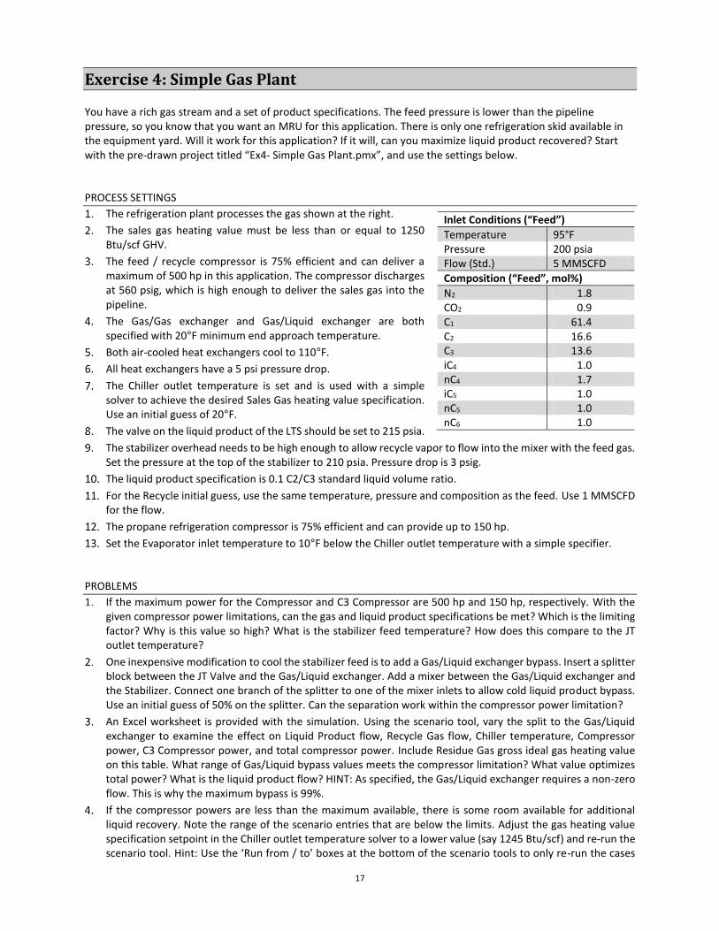
Exercise 4: Simple Gas Plant

You have a rich gas stream and a set of product specifications. The feed pressure is lower than the pipeline pressure, so you know that you want an MRU for this application. There is only one refrigeration skid available in the equipment yard. Will it work for this application? If it will, can you maximize liquid product recovered? Start with the pre-drawn project titled “Ex4- Simple Gas Plant.pmx”, and use the settings below.

PROCESS SETTINGS

The refrigeration plant processes the gas shown at the right.

The sales gas heating value must be less than or equal to 1250 Btu/scf GHV.

The feed / recycle compressor is 75% efficient and can deliver a maximum of 500 hp in this application. The compressor discharges at 560 psig, which is high enough to deliver the sales gas into the pipeline.

The Gas/Gas exchanger and Gas/Liquid exchanger are both specified with 20°F minimum end approach temperature.

Both air-cooled heat exchangers cool to 110°F.

All heat exchangers have a 5 psi pressure drop.

The Chiller outlet temperature is set and is used with a simple solver to achieve the desired Sales Gas heating value specification. Use an initial guess of 20°F.

The valve on the liquid product of the LTS should be set to 215 psia.

The stabilizer overhead needs to be high enough to allow recycle vapor to flow into the mixer with the feed gas. Set the pressure at the top of the stabilizer to 210 psia. Pressure drop is 3 psig.

The liquid product specification is 0.1 C2/C3 standard liquid volume ratio.

For the Recycle initial guess, use the same temperature, pressure and composition as the feed. Use 1 MMSCFD for the flow.

The propane refrigeration compressor is 75% efficient and can provide up to 150 hp.

Set the Evaporator inlet temperature to 10°F below the Chiller outlet temperature with a simple specifier.

PROBLEMS

If the maximum power for the Compressor and C3 Compressor are 500 hp and 150 hp, respectively. With the given compressor power limitations, can the gas and liquid product specifications be met? Which is the limiting factor? Why is this value so high? What is the stabilizer feed temperature? How does this compare to the JT outlet temperature?

One inexpensive modification to cool the stabilizer feed is to add a Gas/Liquid exchanger bypass. Insert a splitter block between the JT Valve and the Gas/Liquid exchanger. Add a mixer between the Gas/Liquid exchanger and the Stabilizer. Connect one branch of the splitter to one of the mixer inlets to allow cold liquid product bypass. Use an initial guess of 50% on the splitter. Can the separation work within the compressor power limitation?

An Excel worksheet is provided with the simulation. Using the scenario tool, vary the split to the Gas/Liquid exchanger to examine the effect on Liquid Product flow, Recycle Gas flow, Chiller temperature, Compressor power, C3 Compressor power, and total compressor power. Include Residue Gas gross ideal gas heating value on this table. What range of Gas/Liquid bypass values meets the compressor limitation? What value optimizes total power? What is the liquid product flow? HINT: As specified, the Gas/Liquid exchanger requires a non-zero flow. This is why the maximum bypass is 99%.

If the compressor powers are less than the maximum available, there is some room available for additional liquid recovery. Note the range of the scenario entries that are below the limits. Adjust the gas heating value specification setpoint in the Chiller outlet temperature solver to a lower value (say 1245 Btu/scf) and re-run the scenario tool. Hint: Use the ‘Run from / to’ boxes at the bottom of the scenario tools to only re-run the cases

Inlet Conditions (“Feed”)

Temperature 95°F Pressure 200 psia Flow (Std.) 5 MMSCFD

Composition (“Feed”, mol%)

N2 1.8 CO2 0.9 C1 61.4 C2 16.6 C3 13.6 iC4 1.0 nC4 1.7 iC5 1.0 nC5 1.0 nC6 1.0

18

that can be improved, as noted previously. If any of the cases are still within the power limits, re-run at a lower GHV. What is the maximum liquid recovery?

Inlet Mixer

Compressor

Air Cooler

Gas/Gas

Gas/Liquid

Chiller

Recycle to Inlet

JT Valve

LTS

Feed

2

3 4 5

6

7

89

10

Reboiler

11

12

Stabilizer

8

1

Q-1

13

14

Sales Gas

Liquid Product

Recycle

Q-2

Q-3

Q-4

Condenser

Evaporator

C3 Compressor

Q-5

VLVE-100

16

1718

19

20

Q-6

TRM-1

MIX-100

Bypass Split

15

2122

19

Plant Processing

In cases where recoveries of propane are desired to be greater than 80%, or when recovery of ethane is desired in

significant quantities in the NGL product, JT and MRU plants will not provide adequate performance. These simple

systems do not get cold enough and do not supply enough stages of separation to get these high rates of liquid

recovery. Historically Lean Oil Absorption and cryogenic JT processes were used to recover deeper cuts of NGL.

However, with the advancements in turboexpander technology, these processes have diminished in importance in

modern gas plants. A simplified version of the cryogenic turboexpander process is shown in Figure 13.

SEPARATOR

EXPANDER

J-T VALVE

BOOSTER

DEMETHANIZER

10

1

4

LIQUID PRODUCT

RESIDUE

FEED

RESIDUE COMPRESSOR

RESIDUE EXCH

INLET EXCH

REBOILER

HEAT

EXCHANGE

NETWORK

Figure 13: Simple Turboexpander Plant

There are four primary distinctions between cryogenic processes and field processes:

1. The products of the cryogenic processes are generally more strictly defined.

2. Rather than a JT valve to expand the gas, the cryogenic process uses a turboexpander. This expander is

mechanically connected to a booster compressor to aid in residue gas compression.

3. The low temperature separator and a stabilizer are effectively combined into one column, typically called

a demethanizer.

4. The heat exchangers are often special high surface area, low temperature, low approach exchangers,

normally referred to as a compact brazed aluminum or plate-fin exchangers.

20

Product Specification Prior to processing, the inlet gas must be suitably treated for operation at low temperature. In order to avoid solids

formation, the gas must be dehydrated so that its hydrate or solids formation dewpoint temperature is lower than

the lowest expected temperature. This will typically be -150 to -200°F. To meet this type of dehydration

specification normally requires a molecular sieve bed. Molecular sieve dehydrators are sensitive to free liquid, so

the gas must be scrubbed and filtered prior to dehydration. The solid sieve material can produce a dust, so the gas

must be filtered again after dehydration to reduce fouling in exchangers. Carbon dioxide can also freeze out at low

temperatures, but will normally be tolerated at levels of approximately 1 mol% depending on the configuration of

the process. Higher levels of carbon dioxide would require acid gas treating prior to dehydration.

The design objective of a cryogenic plant is to cool the inlet gas in order to condense the target natural gas liquids,

while meeting liquid product purity requirements, and minimizing compression horsepower. The two products will

be a demethanized liquid and a lean overhead gas. The demethanized liquid product, commonly referred to as ‘Y-

grade’, typically has the following specifications:

Vapor Pressure: < 600 psig @ 100 °F

Methane / ethane ratio: < 1.5 liquid volume %

Methane content: < 0.50 liquid volume %

ASTM D86 Endpoint: < 275 °F

Carbon dioxide / ethane ratio: < 0.35 liquid volume %

Carbon dioxide content < 1000 ppm wt

Water: No free water at 34°F

The overhead vapor typically has specifications on impurities such as CO2, H2S, and moisture. However, these

specifications are generally met by the pre-processing for cryogenic operation. If not removed prior to processing,

H2S, COS, and mercaptans will be recovered in the liquid product. CO2 will be split between the residue gas and the

ethane. As ethane recovery increases, the carbon dioxide recovery in the ethane will increase. Inlet nitrogen,

helium and hydrogen will be recovered with the residue gas.

An important product specification that impacts the NGL recovery process is final sales gas line pressure. Along

with the available residue gas compression, this dictates the lower limit of the NGL recovery. One other

specification that can have a significant impact on a gas processing plant operation is the heating value of the

product gas. Typical pipeline specifications require a heating value less than 1150 Btu/scf (typically specified as

gross or higher heating value). In the instance that certain NGLs are not economical to recover, this sets a

minimum liquids recovery. For example, 1150 Btu/scf is a common upper limit for heating value. For a

hydrocarbon only blend, this would be met by a methane composition of about 89 mol%. It is important to note

that heating value is significantly affected by relatively small amounts of heavier hydrocarbons. An alternative

specification of heating value is the Wobbe Index.

𝑊𝑜𝑏𝑏𝑒 𝐼𝑛𝑑𝑒𝑥 = 𝐺𝑟𝑜𝑠𝑠 𝐻𝑒𝑎𝑡𝑖𝑛𝑔 𝑉𝑎𝑙𝑢𝑒

√𝑆𝑝𝑒𝑐𝑖𝑓𝑖𝑐 𝐺𝑟𝑎𝑣𝑖𝑡𝑦

The Wobbe Index is considered a slightly better indicator of interchangeability of fuel gases than heating value

alone. Wobbe Index has the same units as heating value. For a natural gas with a gross heating value of 1150

Btu/scf gas and specific gravity of 0.61, it would have a Wobbe Index of 1436 Btu/scf.

The main question that the designer must answer is what fraction of NGL will be recovered from the inlet gas

stream. For a turboexpander plant, 99+% recovery of the C4+ components is normal. For propane, the typical

recovery is 95-99%. The ‘key’ component that dictates overall plant performance is the ethane recovery. The

21

simple turboexpander plant can typically recover 70-80% of the ethane, depending on gas composition and

available compression. More sophisticated demethanizer configurations can recover up to 99% of the ethane.

Figure 14 shows the relationship of propane and butane recovery to ethane recovery for a typical turboexpander.

Propane and heavier component recoveries vary with the equipment arrangement.

Figure 14: Typical Propane and Butane Recovery Relative to Ethane Recovery in a Turboexpander

Once the desired product recovery is determined, the product compositions are set by a simple material balance.

For a hypothetical inlet gas with the listed composition, Table 1 shows the expected products based on typical gas

plant recoveries and a methane:ethane ratio in the liquid product. The bold values indicate product or

performance specifications.

Table 1: Composition of Feed Gas, Liquid Product, and Residue Gas

FEED LIQUID RESIDUE

mol% Recovery mol% Liq vol% mol%

Methane 90.0% 0.09% 1.0% 0.6% 98.2%

Ethane 5.0% 70% 41.5% 39.0% 1.6%

Propane 3.0% 95% 33.8% 32.7% 0.2%

i-Butane 0.4% 100% 4.7% 5.5% 0.0%

n-Butane 1.0% 100% 11.9% 13.1% 0.0%

i-Pentane 0.2% 100% 2.4% 3.0% 0.0%

n-Pentane 0.4% 100% 4.7% 6.0% 0.0%

Total 100.0% 8.4% 100% 100% 100%

GHV (Btu/scf) 1143 --- 2421 --- 1025

Wobbe 1436 --- 2026 --- 1369

If we assume that the residue gas / liquid product separation will be achieved by a distillation column of some sort,

our product compositions give an indication of the conditions in that column. Figure 15 shows the bubble point

85

90

95

100

40 50 60 70 80 90 100

Re

cove

ry (

%)

Ethane Recovery (%)

Butane

Propane

22

curve of our hypothetical liquid product and the dew point curve of our hypothetical residue gas. If we further

assume that the inlet gas will be the heating source for the liquid product reboiler, this sets a temperature /

pressure boundary on the system. For an inlet gas temperature of 100°F and a 10°F approach temperature, the

reboiler must operate at no higher than 90°F and consequently a maximum pressure of 310 psig. If the

hypothetical distillation column can operate no higher than 310 psig, then the dewpoint line of our vapor product

indicates the maximum temperature of the overhead of the column. By this reasoning, the product vapor must be

no higher than -135°F. Again, if the column pressure is lower, the maximum overhead temperature will also be

lower.

Figure 15: Bubble Point of Liquid Product and Dew Point of Vapor Product

Turboexpander The primary concept behind turboexpander plants is to perform the auto-refrigeration of the feed using an

expander rather than a simple valve. By removing energy in the form of work, the resultant expanded gas is

considerably colder than would be achieved using an adiabatic expansion. Beyond the formation of additional

liquids due to lower temperatures, the expander has the added benefit of producing work that is available to be

used for recompression of the residue gas, reducing overall compression costs. Special designs and technologies

are required in the expander turbines themselves as these systems should expect vapor inlet but a multiphase

outlet. Typical gas processing turboexpander outlet temperatures range from -130 to -160°F. The outlet stream

can be up to about 50% liquid by mass and can generate up to 15,000 horsepower in a single unit.

Rather than operating adiabatically like the J-T valve does, the expander operates in a somewhat isentropic

fashion, similar to a compressor. Figure 16 and Figure 17 show the behavior of expanding the same hypothetical

gas from 800 psig to 300 psig using a JT valve and an ideal (isentropic) expander. In each plot, the JT valve takes the

system to 95% vapor, while the expander ends up at approximately 87% vapor. Real expanders are typically 70-

90% polytropic efficient. An expander with 80% polytropic efficiency in this hypothetical case would have an

endpoint of 89% vapor.

0

100

200

300

400

500

600

700

800

-200 -100 0 100 200

Pre

ssu

re (

psi

g)

Temperature (°F)

Dew Pt Vapor

Bub Pt Liquid

23

Figure 16: J-T Valve vs. Expander, Pressure – Enthalpy Diagram

Figure 16 shows the expansion on a pressure / enthalpy field, with the phase behavior of the gas overlaid. The J-T

valve expands the gas along constant enthalpy, while the expander reduces the enthalpy by the shaft work done.

Figure 17 shows the standard pressure-temperature relationship for a phase diagram. As expected, the expander

shows a lower final temperature.

Figure 17: J-T Valve vs. Expander, Pressure – Temperature Diagram

It should be noted that while these two cases are shown to begin at the same temperature and pressure and end

at the same pressure, this would not necessarily be a fair comparison to a real system. Because the expander

provides work for the booster compressor, it can expand to a lower demethanizer pressure for the same residue

gas compressor. A typical booster compressor will increase the residue gas pressure by 40 to 60 psi. If this is taken

into account, the final JT temperature would be about 5°F warmer. In addition, because the demethanizer

overhead temperature would be higher, there is not as much cooling available for the inlet gas in the JT system

compared to the expander. This means that the starting condition for the JT valve would be a higher temperature,

0

100

200

300

400

500

600

700

800

900

-36500 -36000 -35500 -35000 -34500 -34000 -33500

Pre

ssu

re (

psi

g)

Enthalpy (Btu/lbmol)

80% Vapor

90% Vapor

100% Vapor

JT

Expander

0

100

200

300

400

500

600

700

800

900

-200 -150 -100 -50

Pre

ssu

re (

psi

g)

Temperature (F)

80% Vapor

90% Vapor

100% Vapor

JT

Expander

24

with a subsequently higher heavy component content. This would further increase the final expansion

temperature for the JT system.

Figure 18 shows the boundary of the thermodynamic system of the turboexpander process. The streams that cross the boundary of the system are the inlet gas, the residue gas, the liquid product, and the work of the expander.

SEPARATOR

EXPANDER

J-T Valve

BOOSTER

DEMETHANIZER

1

4

LIQUID PRODUCT

RESIDUE

FEED

RESIDUE COMPRESSOR

RESIDUE EXCH

INLET EXCH

REBOILER

HEAT

EXCHANGE

NETWORK

Figure 18: Thermodynamic System of Turboexpander Process

This energy balance can be expressed as:

WEXPANDER = HFEED – HRESIDUE – HLIQUID

In order to increase the liquid recovery, the enthalpy of the products must be reduced (more low-enthalpy liquid

relative to high-enthalpy gas). This leads to a greater enthalpy differential between feed and products and results

in higher expander work required. The work of the expander is dependent on the inlet flow and the pressure ratio

across the expander. For a consistent temperature, pressure, and flow through the separator, the work of the

expander is primarily defined by the expander discharge pressure (tower pressure). For the above configuration

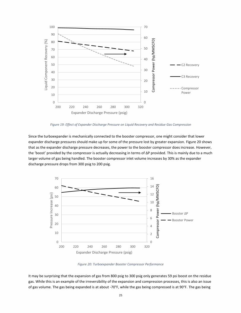
and a defined feed and liquid recovery, the system can be solved by iterating on column pressure. Figure 19 shows

a range of performance for the simple turboexpander process described in Figure 18. For the target recovery of

70% ethane, the expander discharge pressure would be about 290 psig. This operating point would give about 97%

propane recovery (greater than the initial target) and a residue compressor power of about 37 hp per MMSCFD of

inlet gas processed. Recovery of ethane can be increased to 80%, at the expense of approximately 23 hp/MMSCFD

of residue compression. Depending on the feed condition (temperature, pressure, composition), the simple

process shown in Figure 18 may not be able to meet the liquid recovery expectation economically. In such cases, a

process modification is needed, which will be discussed later.

25

Figure 19: Effect of Expander Discharge Pressure on Liquid Recovery and Residue Gas Compression

Since the turboexpander is mechanically connected to the booster compressor, one might consider that lower

expander discharge pressures should make up for some of the pressure lost by greater expansion. Figure 20 shows

that as the expander discharge pressure decreases, the power to the booster compressor does increase. However,

the ‘boost’ provided by the compressor is actually decreasing in terms of ΔP provided. This is mainly due to a much

larger volume of gas being handled. The booster compressor inlet volume increases by 30% as the expander

discharge pressure drops from 300 psig to 200 psig.

Figure 20: Turboexpander Booster Compressor Performance

It may be surprising that the expansion of gas from 800 psig to 300 psig only generates 59 psi boost on the residue

gas. While this is an example of the irreversibility of the expansion and compression processes, this is also an issue

of gas volume. The gas being expanded is at about -70°F, while the gas being compressed is at 90°F. The gas being

0

10

20

30

40

50

60

70

0

10

20

30

40

50

60

70

80

90

100

200 220 240 260 280 300 320

Liq

uid

Co

mp

on

ent

Rec

ove

ry (

%)

Expander Discharge Pressure (psig)

C2 Recovery

C3 Recovery

CompressorPowerC

om

pre

sso

rP

ow

er (

hp

/MM

SCFD

)

0

2

4

6

8

10

12

14

16

0

10

20

30

40

50

60

70

200 220 240 260 280 300 320

Pre

ssu

re I

ncr

ease

(p

si)

Expander Discharge Pressure (psig)

Booster ΔP

Booster Power

Co

mp

ress

or

Po

wer

(h

p/M

MSC

FD)

26

expanded starts at a reference volume of 1 and expands to 2.6, while the gas being compressed goes from a

relative volume of 7.1 to 6.2.

For gas processing, turboexpanders have a single stage with radial inward flow, that is the gas enters the expander

wheel at the outer tips and flows towards the center (centripetal). The gas then exits axially, away from the

compressor side. For the booster compressor the gas path is reversed, entering axially and exiting radially

(centrifugal). Because the boost is only about 30 to 60 psi and the compression ratio is on the order of 1.1 to 1.3, a

single stage of compression is sufficient. Turboexpanders are typically equipped with a JT valve bypass for startup,

excess flow, and expander shutdown conditions. As mentioned previously, the JT valve is not as effective at cooling

the gas as the expander, so it should remain shut during normal operation. A bypass valve leaking by is a possible

source of inefficiency in matching plant and simulator data.

Turboexpander Efficiency

The expander side of a turboexpander is considered to behave in a somewhat adiabatic, reversible (isentropic)

manner. As such, expanders are typically rated using an adiabatic efficiency (ηad). This is defined by the enthalpy

change relative to the isentropic path:

𝜂𝑎𝑑 =𝑊𝑜𝑟𝑘 𝑎𝑐𝑡𝑢𝑎𝑙𝑙𝑦 𝑝𝑟𝑜𝑑𝑢𝑐𝑒𝑑

𝑊𝑜𝑟𝑘 𝑝𝑟𝑜𝑑𝑢𝑐𝑒𝑑 𝑏𝑦 𝑖𝑠𝑒𝑛𝑡𝑟𝑜𝑝𝑖𝑐 𝑝𝑎𝑡ℎ=

𝛥𝐻𝑎𝑐𝑡𝑢𝑎𝑙

𝛥𝐻𝑖𝑠𝑒𝑛𝑡𝑟𝑜𝑝𝑖𝑐

Given inlet conditions and outlet pressure, the isentropic path can be calculated using an equation of state.

In addition to expanders, the adiabatic efficiency is also typically used for reciprocating compressors, inverted due

to compression rather than expansion. However, centrifugal compressors, including the compressor side of a

turboexpander, behave more as a polytropic process, meaning they are governed by a P-V relationship of the form:

𝑃1𝑉1𝑛 = 𝑃2𝑉2

𝑛

Where P is the pressure, V is the specific volume, n is an exponent that is modified depending on behavior. For

adiabatic, reversible (isentropic) compression or expansion, the value that makes the PVn relationship true is

named k, sometimes referred to as the isentropic k. The relationship between the isentropic k and the polytropic n

defines the polytropic efficiency (ηp):

𝜂𝑝 =𝑛(𝑘 − 1)

(𝑛 − 1)𝑘

As polytropic processes, centrifugal compressors, including booster compressors, are typically characterized using

polytropic efficiency. For all compressors and expanders, ProMax reports both the adiabatic and polytropic

efficiency, as well as the values for n and k, regardless of type or specification.

Demethanizer Column The demethanizer acts as a fractionation column to separate the methane or the methane/ethane from the

heavier liquid components. Because of the large volume of methane relative to the liquid components,

demethanizers have a larger diameter upper section where the methane-rich vapor is fed and a smaller diameter

lower section, where much of the liquids product purification occurs.

The methane / ethane distillation split is not difficult in terms of required number of trays. Depending on the feed

gas and product specification, the theoretical minimum number of ideal stages for this separation is typically two

to five. With a common tray efficiency of 45 to 60%, a normal number of actual stages for a demethanizer column

is 18 to 26. The upper stages of a demethanizer (above the LTS liquid feed) are often packed due to a low liquid :

27

vapor ratio. Lower trays are trayed or packed. Demethanizers typically operate in the range of 100 to 450 psig. The

demethanizer operates with a large temperature gradient. The overhead vapor will range from -150 to -175°F,

while the bottoms product will be 0 to 80°F.

The Low Temperature Separator (LTS) serves to remove the liquid from the cooled feed gas stream. This prevents

liquid from entering the expander. Splitting the vapor and liquid feed also puts more of the heavy components

further from the overhead, allowing for more efficient NGL recovery. It is important to note that if the feed gas

pressure is higher than the cricondenbar, the LTS will be single phase. In this case, the LTS will not separate phases.

While a turboexpander cannot tolerate a two-phase feed, it can be designed to handle supercritical ‘dense’ phase

material. The typical temperature for a Low Temperature Separator is -20 to -60°F.

Heat Exchange Because of the cryogenic conditions that are found in a gas processing plant, the heat exchangers are often

different than conventional shell and tube heat exchangers. Rather than carbon or stainless steel, heat exchangers

for cryogenic service are made primarily of aluminum and are rated for conditions as severe as -450°F and 1500

psig. They are more expensive than conventional carbon steel heat exchangers, but they have very large heat

transfer area per volume and can handle several hot and cold streams in a single shell. In addition to their special

fabrication, these exchangers are extensively insulated, including sealing them in an inert container known as a

‘Cold Box’. Figure 13 shows the heat exchangers as a single heat transfer side for each service. In application, each

service (feed, reboiler, and residue) can be multiple exchangers in series. Other design considerations for plate-fin

heat exchangers include clogging potential due to small flow channels, relatively low maximum operating

temperature (<150°F), sensitivity to corrosives, and structural damage from mercury contamination. Proper feed

treatment can eliminate most of these concerns.

For the hypothetical case presented in Table 1, Figure 21 shows the balance between energy supplied by the inlet

gas and the energy demanded by the reboiler and the demethanizer overhead gas. The supply curve is made up of

two relatively straight line segments joined together at approximately 20°F. The higher temperature piece is the

sensible cooling of the gas to its dew point. The lower temperature section is flatter (lower ΔT/ΔH) as it indicates

simultaneous sensible and latent heat removal. While the demand curve encompasses both cooling streams

simultaneously, the two separate effects are apparent. The higher temperature portion of the curve is flatter

(lower ΔT/ΔH) and is dominated by the heat required for the vaporization of the bottoms product in the reboiler.

The much steeper slope of the lower temperature section (<40°F) is simply the sensible heat of the overhead gas.

The first thing that should be noted is that the endpoints represent a rational macroscopic system, that is, THOT >

TCOLD for each end. The next item that is noteworthy is that the supply and demand lines cross in the middle,

indicating an unfeasible situation internal to the heat exchange system.

28

Figure 21: Heat Exchanger Network Energy Balance

This problem of impossible temperature cross could be eliminated by adding an external heat source to provide

reboiler duty at a higher temperature. While heat sources at 100°F are not hard to find, this would negatively

affect the heat balance by requiring more work extracted by the expander, and consequently more compression

power to make up for the pressure loss. A second option would be to provide the reboiler duty at a lower

temperature by inputting some of the energy higher in the column in the form of a side-reboiler. Figure 22 shows

the temperature profile of a demethanizer column without side reboilers. Because of their low liquid

temperatures, trays 6 to 8 would be candidates for the side reboiler draw.

Figure 22: Demethanizer Temperature Profile

Figure 23 shows the process with a side reboiler drawing liquid from stage 6 and returning the partially vaporized

stream to stage 7. The overall heat exchange network could be constructed as a single complex exchanger with

one hot stream and three cold streams. Looking at the system in further detail shows the problem with this

arrangement. Residue gas is available at much lower temperature than the reboiler duty cooling. There is also a

-150

-100

-50

0

50

100

0 5 10 15

Tem

per

atu

re (°F

)

Duty (MMBtu/hr)

Supply

Demand

1

2

3

4

5

6

7

8

9

10

11

-150 -100 -50 0 50 100

Tray

Nu

mb

er (

1=T

op

, 11

=Reb

oile

r)

Temperature (°F)

29

significantly different cooling capacity available in the two services due to mass flow. Finally, the reboiler duty is

typically used as a manipulated variable to control product quality and thus needs to be able to operate

independent of the rest of the system. In order to accommodate this separation, the reboiler and the residue gas

exchanger are shown as separate parallel units. Figure 23 shows the reboiler built as a single complex unit.

Because of the temperature profile of this system, it is normally constructed as separate exchangers in series

contained in the same housing, rather than 3 parallel streams.

SEPARATOREXPANDER

J-T VALVE

BOOSTER

DEMETHANIZER

10

1

4

7

6

LIQUID PRODUCT

RESIDUE

FEED

RESIDUE COMPRESSOR

RESIDUE GAS EXCH

REBOILER

Figure 23: Turboexpander Process with Split Feed and Side Reboiler

Figure 24 shows the performance of the heat exchangers with the split feed and side reboiler. The ‘stair-step’ in

the reboiler demand curve is the changeover between the bottom reboiler and the side reboiler. In this case, there

are no temperature crosses between the supply and demand. However, both curves show examples of close

approach temperatures. This is an example of why the compact brazed aluminum heat exchangers with very high

heat transfer area are needed. Plate fin exchangers are frequently specified with approach temperatures as low as

3°F, as compared to 10 to 15°F for shell and tube.

30

Figure 24: Heat Exchanger Performance for Split Feed and Side Reboiler

Figure 25 shows the impact of the side reboiler on the temperature profile of the demethanizer. Because the vapor

boilup is more distributed in the column, the required diameter of a side-reboiled demethanizer can be less than

the bottom-only reboiler. However, the side-reboiled column will need more physical height to allow space for the

chimney tray and the vapor / liquid disengagement zone for the reboiled material.

Figure 25: Demethanizer Temperature Profile with and without Side Reboiler

-20

0

20

40

60

80

100

0 0.5 1 1.5 2 2.5 3 3.5

Tem

per

atu

re (°F

)

Reboiler Duty (MMBtu/hr)

Supply

Demand

-150

-100

-50

0

50

100

0 2 4 6 8 10 12

Tem

per

atu

re (

°F)

Residue Gas Exchanger Duty (MMBtu/hr)

Supply

Demand

1

2

3

4

5

6

7

8

9

10

11

-150 -100 -50 0 50 100

Tray

Nu

mb

er (

1=T

op

, 11

=Reb

oile

r)

Temperature (°F)

Side Reboiler

No Side Reboiler

31

Exercise 5: Demystifying the Turboexpander Plant

This exercise will demonstrate the logical steps for the development of a turboexpander plant starting with a simple mechanical refrigeration process. It will show that use of the expander provides all of the refrigeration required for the unit. Each step of this exercise will be worked as a group. Open ‘Ex5- ConventionalExpander.pmx’ in the Exercises folder.

PROCESS SETTINGS

Starting with the basic MRU system, replace the JT valve with an expander having 80% efficiency.

Note that the expander is being fed two phases, which is not allowed. Move the separator just downstream of the chiller. Expand the vapors to 250 psig. A valve will be required to lower the pressure of the liquids to 250 psig as well.

Note that we now have two phases in both outlet streams. A convenient way to separate the vapor and liquids of each stream and subsequently recombine is with a column. Add a 2 stage column to the flowsheet, sending the expanded vapors onto stage 1 and the JT liquids onto stage 2. Give the column a 5 psi pressure change.

At this point, we have a vapor and a liquid which are extremely cold leaving the system. We would like to recover some of this “free” refrigeration with heat integration. Let’s start with the liquids from the bottom. If we cross exchange these liquids with the feed gas, we’ll cool the feed and unload the propane chiller. At the same time, we’ll produce some vapors from liquids which will need to be reintroduced to the column. To take care of all of this, add a single sided heat exchanger upstream of the propane chiller, name it “Reboiler Tubes”, and set its outlet temperature to 70°F. Add a kettle reboiler to the column bottoms. Connect the two heat exchangers via their duty stream, effectively creating a cross exchanger. You will also need to specify the Reboiler in the Process Data tab of the Column.

Take a look at the column temperature profile and compare the bottom stage temperature to the reboiler temperature. Additional stages are required, including several between the JT liquid feed and the reboiler. Add stages to get a total of 10 stages in the column. Feed the JT liquid onto stage 3.

Look again at the column profile and notice that from stage 3 to 8, little temperature change is occurring and the fluids on the stages are extremely cold. This is an indication that some additional refrigeration can be recovered via a side reboiler. Add a single-sided heat exchanger in-between the reboiler tubes and the chiller naming it “Side Reboiler”. Set its outlet temperature to 64°F and send its duty stream directly onto stage 6. This effectively makes a cross exchanger between the feed and the fluids on stage 6. Look at the column profile now and notice that a much more reasonable temperature profile is achieved.

The liquids leaving the system are now at a reasonably warm temperature. However, the vapors leaving are still extremely cold. Additional refrigeration recovery is possible by passing these vapors through a single sided heat exchanger. Drop a single sided heat exchanger on the flowsheet, pass the vapors through it and connect the chiller duty to this single sided heat exchanger. You have now completely displaced the propane chiller and the unit is relying solely on the refrigeration achieved through the expander.

Add a residue compressor to the now warmed gas, connecting the power generated from the expander to it.

Inlet Conditions (“Feed”)

Temperature 100 °F Pressure 800 psig Flow (Std.) 50 MMSCFD

Composition (“Feed”, mol%)

C1 90.0 C2 5.0 C3 3.0 iC4 0.4 nC4 1.0 iC5 0.2 nC5 0.4

32

Feed

C3 Chiller

1

Q-1

2

3

LTS

4

Expander

Q-2

K-1005

6

DTWR-100

10

1

2

3

4

5

6

7

8

9

Q-3

7

8

Reboiler Tubes

9

Side Reboiler

Q-4

10

XCHG-101

12 13

CMPR-100

33

Exercise 6: Expander Plant Feed Splits

Up until now, we have used simple and straightforward heat integration. In this exercise, we will set up the splits in the feed gas to provide closer heat integration with appropriate driving forces. Start with the pre-drawn project titled “Ex6- ExpanderPlantOptimization.pmx”, and use the settings below.

PROCESS SETTINGS

Add a split to the feed gas, sending one side through the Gas/Gas Exchanger and the other side through the Reboiler and Side Reboiler, the latter two in series.

Split the feed 40% to the reboilers.

All of the feed recombines before entering the LTS. See the flowsheet below.

The propane refrigeration system only supplies cooling when the LTS temperature rises above -35°F. Set up a specifier with logical operations so that the propane loop only provides cooling when the temperature of the LTS feed is greater than -35°F. If the LTS Feed temperature is less than -35°F, the duty for the propane loop should be zero.

Add a solver on the feed splitter so that the reboiler maintains a 5°F Minimum Effective Approach Temperature.

Add a solver on the Gas/Gas Exchanger outlet temperature so that a 5°F Minimum Effective Approach Temperature is maintained. Use an initial guess of -80°F for the outlet temperature.

Add a solver on the Side Reboiler duty so that it maintains a 5°F Minimum Effective Approach Temperature. Use 2.0 MMBtu/h as an initial guess.

The column operates at 275 psig.

Create specifiers so that the Expander outlet and JT outlets are each 3 psi above their respective feed stages.

Inlet Gas

1

Expander

2

Q-2

LTS

3

4

VLVE-100

5

Demethanizer

10

1

2

6

3

4

5

8

7

9

6

7

Reboiler Tubes

Q-3

K-100

9

Liquid Product

Q-4

Side Reboiler

12

1516

Gas/Gas Exchanger

Booster

Residue Gas

QRCYL-1

Q Q-1

Mixer

Inlet Split

11

13

14

Q-5

C3 Chiller

17

Inlet Conditions (“Feed”)

Temperature 100°F Pressure 800 psig Flow (Std.) 50 MMSCFD

Composition (“Feed”, mol%)

C1 90.0 C2 5.0 C3 3.0 iC4 0.4 nC4 1.0 iC5 0.2 nC5 0.4

34

PROBLEMS

What is the temperature of the fluid leaving the Gas/Gas Exchanger when a 5°F approach is achieved

What is the ethane recovery for this system? Propane recovery?

Does the expander provide sufficient cooling to eliminate the need for the propane refrigeration system?

What is the effect on ethane and propane recoveries if a 5 psi pressure drop is assumed for the Reboiler Tubes, Side Reboiler, Gas/Gas Exchanger, and LTS?

What is the effect on ethane and propane recovery if the expander operates at 72% efficiency instead of 75%?

Add a Residue Compressor (75% polytropic efficiency) to the Residue Gas stream. Note the power. Reduce the pressure in the demethanizer from 275 psig to 265 psig. What happens with ethane recovery and Residue Compressor power?

OPTIONAL: At times it is useful to show shaft losses in the expander / compressor system, typically on the order of 1 to 2% of the work. Note the discharge pressure of the booster compressor. Disconnect the expander energy stream from the compressor. Add a second energy stream to the compressor. For the new energy rate, specify 98.5% of the expander energy rate. What happens to the ethane recovery in the process? How much does the booster compressor discharge pressure change?

35

Turboexpander Variations While Figure 23 shows the basic turboexpander process, there are a great number of process variations due to

feed gas, product specifications, and existing equipment limitations. The three variations described below are not

an exhaustive list, but capture a large portion of the major differences.

Mechanical Refrigeration

If an inlet gas stream is very rich in liquids content, the amount of latent heat that must be removed in the form of

expander shaft work can be significant. This high shaft work requires a low column pressure and consequently high

recompression power. In this case, it can be more economical to remove some of the condensation energy via

mechanical refrigeration. The most common form of refrigeration in gas processing is the propane cycle described

previously. This has a low end temperature of -25 to -35°F. For a conventional turboexpander plant with an LTS

temperature of -50 to -60°F, this would require breaking the residue or gas/gas exchanger into two pieces, a warm

gas-gas exchanger and a cold gas-gas exchanger with the propane chiller in between. This is shown in Figure 26. A

guideline for adding mechanical refrigeration is if the inlet gas liquids content (C2+) is greater than 3 gallons per

MSCF.

Inlet Gas

Splt-1

2

5

6

Mix-1

7

8

4

From Demethanizer Ovhd12To Booster

Warm Gas/Gas Cold Gas/Gas

C3 Chiller

3

LTS

Reboiler

Q-1

Q-2To Expander

To JT Valve

Figure 26: Location of Mechanical Refrigeration in Turboexpander System

Similarly, if the inlet gas has insufficient pressure to provide enough auto-refrigeration, mechanical refrigeration

can be used to increase liquids recovery. A guideline for when this becomes economical is when the inlet gas

pressure is below about 700 psig.

GSP Process

For a given demethanizer pressure the amount of ethane recovered from a feed stream is somewhat dependent

on the temperature at the top of the demethanizer. If a portion of the high pressure feed gas were cooled by the

very cold demethanizer overhead gas, the stream resulting from the expansion of that pre-cooled gas could

provide an even lower temperature than the normal expander outlet. In choosing a stream for this extreme

cooling, it is important to remember that the LTS vapor has had a significant amount of the liquids removed from

it, making it leaner than the total feed stream. This separator overhead gas is a saturated vapor, so any cooling will

cause some condensation. This type of multi-phase stream is not feasible as a feed to a high-speed turbine.

However, with sufficient pre-cooling a J-T valve in this application can generate a lower temperature than the

existing expander. This is the basis of the Ortloff Gas Subcooled Process (GSP), which was patented in 1977. A

simplified version of this process is shown in Figure 27. As the name implies, a portion of the LTS vapor is

condensed and subcooled. This process can recover more ethane with less recompression power than would be

possible with a conventional turboexpander process. This scheme can economically recover up to about 90% of the

36

ethane in the feed stream, depending on inlet gas conditions. The main cost associated with this enhancement is

the addition of the Subcooler and the extension of the largest diameter section of the demethanizer to handle two

feeds.

LTS

EXPANDER

J-T VALVE

BOOSTER

LIQUID PRODUCT

RESIDUE

FEED

RESIDUE COMPRESSOR

RESIDUE GAS EXCH

REBOILER

SUBCOOLER

J-T VALVE

DEMETHANIZER

Figure 27: Simplified GSP Turboexpander Process

With some of the LTS vapor routed to the Subcooler, the expander will see fewer moles of gas in the GSP process

as compared to the conventional turboexpander. This makes the improved performance of the GSP somewhat

counterintuitive. For a demethanizer operating at the same pressure, the temperature and pressure of the gas and

liquid products are essentially the same for both cases. If the GSP process can produce more liquid, then by the

simple energy balance the extra enthalpy removal must come from extra shaft work of the expander. However,

the expander pressure drop is the same for both cases, but only a fraction of the LTS vapor is passing through the

expander in the GSP case. Because some of the cold overhead stream is being used to subcool LTS vapor, there is

not as much cooling available for the inlet gas. As such, the LTS temperature runs significantly higher than the

conventional turboexpander process. These trends are shown in Figure 28. The expander work is determined

substantially by the actual inlet volumetric flow and the pressure ratio. As such, for a specific range of LTS split,

the expander work is higher for the GSP than for the conventional turboexpander. The expander work typically

maximizes with a split in the range of 30 mol%. Too much flow to the Subcooler and the net autorefrigeration

suffers by using too much JT and not enough expander.

37

Figure 28: GSP Performance vs. LTS Vapor Split

A further advantage of this process is enhanced operating stability because the LTS is warmer, and thus farther

away from the potentially troublesome all-liquid phase boundary. In addition to the subcooling of a portion of the

LTS vapor, it is also part of the GSP process to allow the flexibility to add some of the LTS liquid to the LTS vapor

going to the Subcooler. This can be helpful for improving the liquid recovery in the case of rich inlet gases (>3

gallons NGL per MSCF). The colder overhead temperature also makes the GSP better suited for propane recovery

in ethane rejection mode. A final advantage of the GSP process relative to the conventional turboexpander process

is increased tolerance to carbon dioxide in the feed, reported to be around 1% due to increased liquid flow at the

top of the column.

The GSP Subcooler is typically simulated with an approach temperature similar to that of the Gas/Gas exchanger,

around 5°F. For an initial guess of the temperature of the subcooled liquid exiting the Subcooler, use the bubble

point of the stream less 20°F. Because the bubble point is strongly dependent on the light ends of the stream, for

an accurate estimate of the bubble point, one can use the inlet gas stream composition.

RSV Process

While the GSP provides a colder top tray liquid feed stream to the demethanizer, it is still a feed stream. This

makes the demethanizer a sophisticated stripper, without a true rectification section. Because of this, the GSP

process is limited to the low to mid 90’s in ethane recovery percentage. If a portion of the overhead gas stream

were condensed and returned to the top of the column, the purification of the methane product (and consequent

ethane recovery) would be more effective because of a true reflux behavior. This concept is demonstrated in the

Ortloff Recycle Split-Vapor (RSV) process, shown in Figure 29. The RSV process was patented in 1994. The

distinction of the RSV from the GSP is that a portion of the residue gas is recycled back through the Subcooler,

where it is cooled by cold demethanizer overhead vapor and flashed to the top of the demethanizer column as

reflux. The purified reflux allows economic ethane recovery of 90 to 98%.

-80.00

-60.00

-40.00

-20.00

0.00

20.00

40.00

60.00

80.00

100.00

0 10 20 30 40 50

LTS Vapor Split (%)

Ethane Recovery %

Expander Inlet (mol% Feed)

LTS Temp (°F)

4.0

6.0

8.0

10.0

12.0

14.0

16.0

0 10 20 30 40 50

LTS Vapor Split (%)

Expander Power (hp/MMSCFD Feed)

Expander Inlet (MCFD/MMSCFD Feed)

38

LTS

EXPANDER

BOOSTER

LIQUID PRODUCT

RESIDUE

FEED

RESIDUE COMPRESSOR

RESIDUE GAS EXCH

REBOILER

SUBCOOLER

DEMETHANIZER

Figure 29: Demethanizer with True Reflux Stream (RSV)

The typical amount of gas recycled back as reflux is around 10% of the residue gas. For cases of high ethane

recovery, the RSV process can recover more ethane than GSP for the same residue compression power, or it can

recover the same ethane with less residue compression, despite the fact that the RSV requires a higher quantity of

residue gas be compressed than the GSP for any level of performance. In order for more moles of gas to require

less power to compress to the same discharge pressure, it requires a higher inlet pressure. This causes both a

lower compression ratio and lower inlet actual volume. For a high enough purity requirement, the RSV reflux

allows the demethanizer to operate at a higher pressure than for a comparable recovery in a GSP.

The process benefits that were true for the GSP process are true to a greater extent for the RSV: greater ethane

recovery, greater propane recovery in ethane recovery and rejection modes, higher carbon dioxide tolerance, and

operation of the LTS further from feed phase instability. The main capital costs associated with the RSV process is

the further extension of the widest portion of the demethanizer, the addition of a third side of the subcooler

exchanger, and the additional residue compression. However, the RSV process does add a degree of flexibility. In

practice, turning off the residue recycle stream will cause the process to operate as the GSP process. In a ProMax

simulation, the top tray of a column must always have a non-zero liquid feed.

The RSV subcooler is typically operated as a true three-sided exchanger. That is, the cold residue gas

simultaneously exchanges heat with the LTS vapor and the recycle gas. With this configuration, the outlet

temperatures of the LTS vapor and the recycle gas will be the same. For most compositions and pressures, the

recycle gas will be above the cricondenbar, so there will be no phase change or subcooling behavior, so the initial

temperature guess should come from the LTS vapor.

39

In traditional refluxed distillation columns, the reflux returns to the thermodynamic system as a liquid. This

necessarily means the heat of vaporization has been removed. In an RSV process, the recycled residue gas returns

to the thermodynamic system as a vapor. This gas has the same composition as the residue gas leaving the

Gas/Gas exchanger. However, the temperature of the recycled gas is typically higher, say 120°F as compared to

the gas leaving the Gas/Gas exchanger of around 90°F. Depending on the pressures, the enthalpy of the recycled

gas can be higher than the residue gas. This can significantly shift the energy balance of the process. Figure 30

shows the pressure relationship of recycle gas (y-axis) and residue gas (x-axis) where the enthalpy of a pure

methane stream would be equal. If the RSV process operates above this line, enthalpy is removed from the system

and the recycle cools the process. If the operating point is below this line, the recycle is actually increasing the

enthalpy of the system. According to this graph, a lower demethanizer pressure and a higher residue compressor

discharge pressure would tend to increase enthalpy removal from the process in the form of reflux cooling, which

should lead to better RSV performance.

Figure 30: Line of Equal Enthalpy for Methane (120°F Recycle / 90°F Residue)

Figure 31 shows the difference in performance of a GSP and RSV process for a hypothetical gas plant. Performance

will vary based on inlet gas conditions, equipment, and product specifications. For the range of high ethane

recovery examined, the RSV has higher recovery for the same compressor power. In addition, the CO2 tolerance of

the RSV process is higher. Both of these phenomena are because the RSV demethanizer can operate at higher

pressure for the same ethane recovery, due to the purity of the reflux stream. In cases where high ethane

recovery is not required, the GSP performance will be equivalent to RSV, or surpass it, because the high purity

reflux is not required.

700

750

800

850

900

950

1000

200 250 300 350 400

Rec

ycle

Pre

ssu

re (

psi

g)

Overhead Pressure (psig)

Cooling

Heating

40

Figure 31: Comparison of GSP and RSV Process

90

91

92

93

94

95

96

97

98

99

100

50 60 70 80 90 100

C2

Rec

ove

ry (

%)

Residue Compressor Power (HP/ MMSCFD)

RSV

GSP

80

82

84

86

88

90

92

94

96

98

100

0.5 1 1.5 2

C2

Rec

ove

ry (

%)

CO2 in Feed Gas (mol%)

GSP

RSV

41

Exercise 7: Expander Plant Reflux Configurations

Follow the outlined steps to compare the performance of the conventional expander, GPS, and RSV plant designs. Start with the pre-drawn project titled “Ex7- ExpanderPlantRefluxConfigurations.pmx”, and use the settings below.

PROCESS SETTINGS

GENERAL

This exercise uses a conventional turboexpander model and is already completed for your reference. There is no propane / LTS chilling.

The expander is 85% adiabatic efficient.

Compressors are 75% polytropic efficient.

The final residue pressure is 800 psig.

The demethanizer in all three cases operates at 265 psig at the top stage.

For the sake of this comparison, all heat exchangers and separators are assumed to have zero pressure drop.

TURBOEXPANDER

Add a “Stream’s Cn+ GPM” liquids property stencil pointing to the Feed. Set the minimum carbon number to 2.

GSP

Solvers for all of the heat exchangers, except the subcooler, have been set up.

Using the splitter for the LTS vapor, route 25% of the vapor through the subcooler and the remainder to the expander.

Connect the expander outlet to stage 4 of the demethanizer. Add a specifier to the expander outlet stream to set its pressure 2 psi higher than its feed stage.

The GSP reflux leaving the subcooler will pass through a JT Valve and enter the demethanizer on stage 1.

Add a Phase Envelope analysis to the Feed stream to estimate the temperature of the liquid leaving the subcooler. The subcooled liquid should be 20°F less than the bubble point of the Feed. Create a solver that adjusts this temperature to give a 5°F Minimum Effective Approach Temperature in the subcooler.

Add a specifier to the flashed reflux stream to set the pressure 2 psi higher than the top stage of the demethanizer.

RSV

The RSV system starts where GSP left off. All heat exchanger solvers except the subcooler have been set up for you.

Configure the LTS vapor split to be 25% to the subcooler. The GSP reflux should enter the demethanizer at stage 2. Add a specifier to make its pressure 2 psi higher than the stage it is feeding.

Add a side to the subcooler.

The residue gas is compressed to 800 psig and is subsequently cooled to 120°F.

The recycle stream is 5% of the total residue compressor discharge and is sent to the subcooler. A recycle block is required. For an initial guess of the flow, use 5% of the methane in the Feed. As an approximation, pure methane can be used for the composition. Temperature and pressure should correspond to the cooled residue compressor discharge.

Create a specifier to make the temperature of the recycle gas leaving the subcooler the same as the GSP reflux.

The RSV reflux will exit the subcooler, travel through a valve, and enter the demethanizer on stage 1. Add a specifier to make the pressure out of the valve 2 psig higher than the column top pressure.

Inlet Conditions (“Feed”)

Temperature 100°F Pressure 800 psig Flow (Std.) 50 MMSCFD

Composition (“Feed”, mol%)

C1 90.0 C2 5.0 C3 3.0 iC4 0.4 nC4 1.0 iC5 0.2 nC5 0.4

42

PROBLEMS

GENERAL

Based on the C2+ GPM value, is this process a candidate for external refrigeration?

How does the ethane recovery compare between the three configurations? Propane?

How does the residue compressor power compare between the three configurations? Expander power?

GSP

The LTS vapor split was initially 25%. Re-run the simulation at 30% to compare ethane recovery and residue compressor power. Repeat the run at 35%. Which split gives the highest ethane recovery? Lowest power demand?

Set the LTS vapor split to 30%. If the column pressure for the GSP system increases to 275 psig, what happens to ethane recovery? Adjust the pressure of the GSP demethanizer column to find where its ethane recovery will equal the conventional turboexpander. How does the residue compressor power compare?

RSV

With a 25% LTS Vapor split, how much is ethane recovery changed when the RSV split is increased to 10%? What is the additional cost in compression power?

Re-run the simulation with a 30% LTS Vapor split and a 5% residue recycle. Is the RSV system more or less effective at increasing ethane recovery with the higher LTS Vapor split?

Check the RSV heat exchangers for thermal stress problems (max approach T > 55°F).

OPTIONAL: Adjust the pressure of the demethanizer column to find where ethane recovery will equal that of the GSP at 265 psig. How does the residue compressor power compare?

Feed

1

Expander 2

Q-Exp

LTS

3

4

VLVE-100

5

Demethanizer

14

1

11

5

8

2

6

7

Reboiler Tubes

Q-3

K-100

9

Liquid Product

Q-4Side Reboiler

12

15

16

Gas/Gas Exchanger

Residue Compressor

8

QRCYL-1

Q Q-1

MixerFeed Split

11

13

14

Subcooler

17

LTS VaporSplit

Air Cooler

18

Q-6

Q-7

19

20

21

RSV Reflux

22

RSV SplitResidue Gas

24

Residue Recycle

25

26

GSP Reflux

27

Booster

29

43

Exercise 8: GSP Plant Optimization - Introduction

Upon receiving a GSP plant simulation, you observe that the reboiler (K-100) has its heat release curve type set to ‘plug flow’, which would be correct for a compact brazed aluminum exchanger. However, you recognize that the existing reboiler is a kettle type. You also get more accurate turbo-expander performance information from the vendor. The Booster compressor polytropic efficiency is now 80% and the Expander adiabatic efficiency is 85%. The Residue Gas pressure is also changed to 384 psig so the model should be adjusted so that the Booster compressor discharge Pressure is also at 384 psig.

There are two interesting notes about this plant. First, there is no residue compressor, so all recompression must be performed by the booster. The second is that due to a material constraint, the LTS must be no colder than -18°F. In practice this is controlled by bypassing inlet gas around the gas/gas exchanger.

Start with the pre-drawn project titled “Ex8- GSPPlantOptimization - Introduction.pmx”, and follow the instructions below. Keep in mind the following tendencies:

1. Increasing flow through a rated exchanger will increase the calculated pressure drop through that side.

2. Increasing flow through an exchanger with a specified duty will increase the approach temperature of the exchanger.

3. Reducing duty for an exchanger with fixed flows will increase the approach temperature of the exchanger.

4. To eliminate pressure drop warnings through rated exchangers, increase the specified pressure drop higher than the calculated value.

5. Increasing the suction pressure of a compressor with a fixed power will increase the discharge pressure.

6. Increasing the power of a compressor with a fixed suction pressure will increase the discharge pressure.

PROCESS SETTINGS

Open the kettle reboiler shape (K-100) and change the Heat Release Curve Type to ‘Pool Boiling’.

Change the expander efficiency to 85% adiabatic.

Change the booster compressor efficiency to 80% polytropic.

The reboiler and subcooler have been rated and will calculate a pressure drop when those ratings are solved.

The column bottoms product specification sets the reboiler duty.

The duty in the gas/gas exchanger is calculated based on the LTS temperature.

The column pressure is set by the expander outlet pressure.

To bring the simulation back to a feasible state, adjust the following variables:

a. LTS vapor split to the subcooler b. Inlet split fraction to the reboiler c. Upper and lower side reboiler exchanger duties d. Expander outlet pressure e. Heat exchanger side pressure drops f. Temperature of reflux exiting the subcooler

Make sure after all adjustments are made that:

a. All heat exchanger minimum effective approach temperatures exceed 2°F. b. Heat exchanger side pressure drop calculations do not exceed user specifications

PROBLEMS

What are the C2 and C3 recoveries?

Inlet Conditions (“Inlet Gas”)

Temperature 115°F Pressure 810 psig Flow (Std.) 60 MMSCFD

Composition (“Inlet Gas”, mol%)

N2 0.70 CO2 0.50 C1 91.30 C2 4.50 C3 1.50 iC4 0.60 nC4 0.40 iC5 0.20 nC5 0.10 nC6 0.15 nC7 0.05

44

What are the minimum end approach temperatures for all heat exchangers?

What is the lowest stream temperature?

How much power is the expander delivering to the compressor?

OPTIONAL: For the above limitations, what set of parameters maximizes liquid product?

Inlet Split

4

5

Reboiler 6

Q-2

Side Reboilers

K-10078

Demethanizer

22

1

4

8

11

12

16

17

Liquid Product

Mixer

11

12

13

LTS

14

15

LTS VaporSplit

16

Subcooler

17

Reflux VAlve

18

19

Expander

20

2122

23

Q-4

Booster Compressor

Residue Gas

JT Valve

25

26

27

28

29

Gas / Gas Exch

Inlet Gas

45

Exercise 9: GSP Plant Optimization – Pumparounds

Objective: Convert pumparound heat exchangers from having fixed duty specifications to having constant UA across all operating conditions.

The starting point simulation has been modified from the previous exercise. Originally, the pumparounds were managed in a compact heat exchanger where the lower pumparound duty was 700 Mbtu/h and the upper was 1.29 MMBtu/h. The compact exchanger has been replaced by an equivalent pair of 2-sided exchangers having the same pressure drop and duty specifications.

Start with the pre-drawn project titled “Ex9- GSPPlantOptimization - Pumparounds.pmx”, and follow the instructions below.

PROCESS SETTINGS

Record the Effective UA for each pumparound exchanger (Upper and Lower Side Reboilers). These will be used in UA solvers later.

Create two Q-Streams. One (lower) should have an Energy Rate of 700 MBtu/h. The other (upper) should be set to 1.29 MMBtu/h. Add two new single-side exchangers which will become the single-sided versions of the current pumparound exchangers (Side Reboiler). Pressure drops for both new exchangers should be set to 5 psi.

Disconnect the pumparound draw and return streams for the lower pumparound from the demethanizer. Attach the lower pumparound Q-stream to stage 17. Disconnect the inlet gas process streams from the original 2-sided exchanger and attach them to the new single-sided lower pumparound exchanger

Solve the model and record the effective UA for the new lower pumparound exchanger.

Create a solver which adjusts the lower pumparound energy stream’s energy rate to maintain the lower pumparound exchanger effective UA to the original lower pumparound’s effective UA. Check the “Skip Dependency Check” box. Note the duty

Repeat steps 3 to 5 for the upper pumparound exchanger.

PROBLEMS

Disconnect the lower pumparound energy stream and reconnect it to stage 16 of the demethanizer. Record the duty. Which configuration produces a duty nearest the original lower pumparound exchanger duty? Note that when the energy stream is disconnected, the solver must be re-specified. Return the energy stream to stage 17. Repeat this test for the upper pumparound energy stream.

Inlet Conditions (“Inlet Gas”)

Temperature 115°F Pressure 810 psig Flow (Std.) 60 MMSCFD

Composition (“Inlet Gas”, mol%)

N2 0.70 CO2 0.50 C1 91.30 C2 4.50 C3 1.50 iC4 0.60 nC4 0.40 iC5 0.20 nC5 0.10 nC6 0.15 nC7 0.05

46

Inlet Gas Split

4

5

Reboiler

6

Q-2

K-10078

Demethanizer

22

1

4

8

11

12

16

17

Liquid Product

Mixer

11

12

13LTS

14

15

LTS VaporSplit

16

Subcooler

17

Reflux Valve

18

19

Expander

20

2122

23

Q-4

Booster

Residue Gas

JT Valve

25

Gas/Gas Exch

Inet Gas

1

Q-Upper

Q-Lower

Upper Side Reboiler

Lower Side Reboiler

47

Exercise 10: GSP Plant Optimization – Rated Exchangers

Objective: Build Solvers to drive Rated Exchanger’s Fraction Overdesign (FOD) to zero. Also build a solver to adjust the Expander outlet pressure to maintain the target Residue Gas pressure.

Start with the pre-drawn project titled “Ex10- GSPPlantOptimization - Rated Exchangers.pmx”, and follow the instructions below.

PROCESS SETTINGS

The inlet split to the reboiler is initially set with a user specification for the fraction to stream 5. Add a solver to that property. Add the “Fraction Over Design” (FOD) for Reboiler/K-100 as a measured variable.

a. Configure the residual error equation such that FOD is zero at the solution.

b. Enable the “Skip Dependency Check” option. Modify the weight of this solver to facilitate convergence.

The subcooler has a temperature specification on its reflux outlet (Stream 17). Add a solver to that property. Add the FOD for the subcooler as a measured variable.

a. Configure the residual error equation such that FOD is zero at the solution.

b. Enable the “Skip Dependency Check” option. Modify the weight of this solver to facilitate convergence.

The LTS Vapor Split to reflux (stream 16) is user specified. Add a Solver to that property. Add the pressure of the residue gas a measured variable.

a. Configure the residual error equation such that the residue gas pressure is 384 psig at the solution. b. Enable the “Skip Dependency Check” option. Modify the weight of this solver to facilitate convergence.

PROBLEMS

Note how the three feeds to the demethanizer that originate from the Feed are all set by the pressure in stream 20 or maintain relative pressure through use of simple specifiers. The demethanizer top stage pressure is also related to the Expander outlet pressure. Now the expander outlet pressure in stream 20 may be adjusted and the rest of the simulation will respond by keeping the residue gas pressure at 384 psig. The exchangers specified by UA maintain the original values and all of the rated exchanger FOD’s are equal to zero.

Raise the Expander outlet pressure from 324 psig to 325 psig. How long does it take for the simulation to converge? Does more or less LTS vapor flow through the turboexpander? Which direction do ethane and propane recoveries move? Does this change increase or decrease the power generated by the Expander and delivered to the Compressor?

Inlet Conditions (“Inlet Gas”)

Temperature 115 °F Pressure 810 psig Flow (Std.) 60 MMSCFD

Composition (“Inlet”, mol%)

N2 0.70 CO2 0.50 C1 91.30 C2 4.50 C3 1.50 iC4 0.60 nC4 0.40 iC5 0.20 nC5 0.10 nC6 0.15 nC7 0.05

48

Exercise 11: GSP Plant Optimization – Vary Outlet Pressure Scenario

Observe several key properties in response to running a Scenario where pressure is raised in 2 psi increments from 305 to 335 psig. The model should reliably converge. The errors in exchangers FOD’s, UA’s and residue pressure should be negligible at each pressure. Plots of ethane and propane recovery versus Expander outlet pressure should be fairly smooth.

Start with the pre-drawn project titled “Ex11- GSPPlantOptimization -Vary Outlet Pressure Scenario.pmx”, and follow the instructions below.

PROCESS SETTINGS

Add an Excel Workbook, Open Scenario Tool.xla, and name the scenario.

Set up Excel with a column for expander outlet pressure from 305 to 335 psig by 2 psi increments. Make columns for receiving scenario outputs with columns titled:

a. Solve Status b. C2 Recovery c. C3 Recovery d. Upper Side Reboiler UA e. Lower Side Reboiler UA f. Reboiler FOD g. Subcooler FOD h. Residue Pressure i. Reboiler Split j. LTS Vapor Split k. Expander Power l. Demethanizer Overhead Temperature m. Liquid Product C2 BPD n. Liquid Product C3 BPD

Add an input variable to Stream 20 pressure which should be user specified. This is the expander outlet pressure to stage 4 of the Demethanizer.

Add output variables for each of the properties mentioned above and associate it with the corresponding Excel ranges.

Run the scenario and observe the results.

PROBLEMS

Plot ethane and propane recoveries versus Expander outlet pressure. At which pressure is ethane recovery maximized? What about propane?

Plot the inlet split to the reboilers and the reflux split versus expander outlet pressure. Which split fraction moves the most over the pressure range?

Plot Demethanizer overhead temperature and expander power versus expander outlet pressure.

OPTIONAL: Which tray shows the highest vapor flow (lbmol/hr)? Which tray has the highest flooding percentage? Does varying the expander outlet pressure by 10% (335 to 305 psig) risk column flooding?

Inlet Conditions (“Feed”)

Temperature 115°F Pressure 810 psig Flow (Std.) 60 MMSCFD

Composition (“Feed”, mol%)

N2 0.70 CO2 0.50 C1 91.30 C2 4.50 C3 1.50 iC4 0.60 nC4 0.40 iC5 0.20 nC5 0.10 nC6 0.15 nC7 0.05

49

Exercise 12: GSP Plant Optimization – Off Design Economic Optimization

Evaluate the economic effects on the previous ProMax Scenario Tool run and justify the most appropriate plant design. Start with the pre-drawn project titled “Ex12- GSPPlantOptimization – Off Design Economic Optimization”, and follow the instructions below.

One calculation of gas plant performance is Keep-Whole value. The return from processing gas is the value of liquid products less the fuel value of those products:

Keep-Whole Value = Liquid Product [bbl/day] * ( Liquid Value [$/bbl]

– Heating Value of Liquid Product [MMBtu/bbl] * Fuel Value [$/MMBtu])

In the calculations below, please note that the calculated values are in units of [$/day]. The constants in the expressions are:

42 gal/bbl 2.79 MMBtu/bbl of C2 3.85 MMBtu/bbl of C3

PROCESS SETTINGS

PART 1

In Excel, store these values each in their own cells:

a. C2 Price = $0.53/gal b. C3 Price = $1.40/gal c. T&F = $0.10/gal (transportation & fractionation) d. Fuel Value = $4.00/MMBtu

Build the following equations in columns so that they are calculated at each level of Expander Outlet Pressure:

a. C2 Value = “Liquid Product C2 BPD” * (42 * (“C2 Price” – “T&F”) - 2.79 * “Fuel Value”)

b. C3 Value = “Liquid Product C3 BPD” * (42 * (“C3 Price” – “T&F”) - 3.85 * “Fuel Value”)

c. Keep Whole Value = C2 Value + C3 Value

PART 2

Increase the Inlet Gas flow rate from 60 to 65 MMSCFD. Solve the ProMax Scenario Tool at the new feed rate.

PROBLEMS

PART 1

Plot Keep-Whole Value and expander power against expander outlet pressure. Add a horizontal line at 770 hp to represent the high limit on expander power. Which is the best expander outlet pressure to run at? What are the corresponding suggested set-points for the reboiler split and the reflux split?

Change C2 Price to $0.10/gal. What is the best operating pressure now?

PART 2

Now what is the economically optimum expander outlet pressure? What is the optimum expander outlet pressure that maintains the expander power below its high limit?

Inlet Conditions (“Feed”)

Temperature 115°F Pressure 810 psig Flow (Std.) 60 MMSCFD

Composition (“Feed”, mol%)

N2 0.70 CO2 0.50 C1 91.30 C2 4.50 C3 1.50 iC4 0.60 nC4 0.40 iC5 0.20 nC5 0.10 nC6 0.15 nC7 0.05

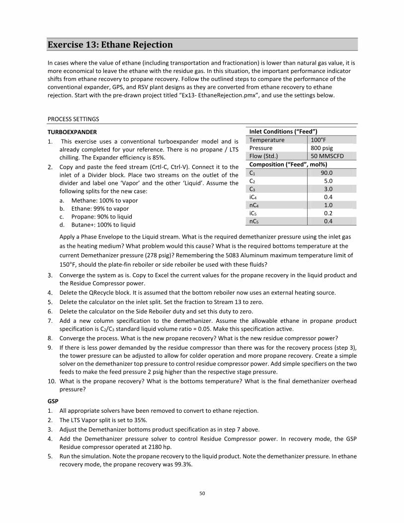
50

Exercise 13: Ethane Rejection

In cases where the value of ethane (including transportation and fractionation) is lower than natural gas value, it is more economical to leave the ethane with the residue gas. In this situation, the important performance indicator shifts from ethane recovery to propane recovery. Follow the outlined steps to compare the performance of the conventional expander, GPS, and RSV plant designs as they are converted from ethane recovery to ethane rejection. Start with the pre-drawn project titled “Ex13- EthaneRejection.pmx”, and use the settings below.

PROCESS SETTINGS

TURBOEXPANDER

This exercise uses a conventional turboexpander model and is already completed for your reference. There is no propane / LTS chilling. The Expander efficiency is 85%.

Copy and paste the feed stream (Crtl-C, Ctrl-V). Connect it to the inlet of a Divider block. Place two streams on the outlet of the divider and label one ‘Vapor’ and the other ‘Liquid’. Assume the following splits for the new case:

a. Methane: 100% to vapor b. Ethane: 99% to vapor c. Propane: 90% to liquid d. Butane+: 100% to liquid

Apply a Phase Envelope to the Liquid stream. What is the required demethanizer pressure using the inlet gas

as the heating medium? What problem would this cause? What is the required bottoms temperature at the

current Demethanizer pressure (278 psig)? Remembering the 5083 Aluminum maximum temperature limit of

150°F, should the plate-fin reboiler or side reboiler be used with these fluids?

Converge the system as is. Copy to Excel the current values for the propane recovery in the liquid product and the Residue Compressor power.

Delete the QRecycle block. It is assumed that the bottom reboiler now uses an external heating source.

Delete the calculator on the inlet split. Set the fraction to Stream 13 to zero.

Delete the calculator on the Side Reboiler duty and set this duty to zero.

Add a new column specification to the demethanizer. Assume the allowable ethane in propane product specification is C2/C3 standard liquid volume ratio = 0.05. Make this specification active.

Converge the process. What is the new propane recovery? What is the new residue compressor power?

If there is less power demanded by the residue compressor than there was for the recovery process (step 3), the tower pressure can be adjusted to allow for colder operation and more propane recovery. Create a simple solver on the demethanizer top pressure to control residue compressor power. Add simple specifiers on the two feeds to make the feed pressure 2 psig higher than the respective stage pressure.

What is the propane recovery? What is the bottoms temperature? What is the final demethanizer overhead pressure?

GSP

All appropriate solvers have been removed to convert to ethane rejection.

The LTS Vapor split is set to 35%.

Adjust the Demethanizer bottoms product specification as in step 7 above.

Add the Demethanizer pressure solver to control Residue Compressor power. In recovery mode, the GSP Residue compressor operated at 2180 hp.

Run the simulation. Note the propane recovery to the liquid product. Note the demethanizer pressure. In ethane recovery mode, the propane recovery was 99.3%.

Inlet Conditions (“Feed”)

Temperature 100°F Pressure 800 psig Flow (Std.) 50 MMSCFD

Composition (“Feed”, mol%)

C1 90.0 C2 5.0 C3 3.0 iC4 0.4 nC4 1.0 iC5 0.2 nC5 0.4

51

Create a Scenario Tool to study a range of LTS vapor splits from 10 to 40% every 5% to examine propane recovery. Include as an input variable Scenario Tool Properties-Flowsheet to Solve What is the maximum propane recovery operating point?

RSV

The RSV system has been prepared similarly to the GSP.

The LTS vapor split is 25%. The residue recycle split is 10%.

Add the C2/C3 bottoms product specification to the demethanizer.

The reference residue compressor power is 2313 hp. Add a solver to the demethanizer pressure to maintain this power. Make the solver a priority of 1.

The Gas/Gas heat exchanger and the Subcooler solvers should have a priority of 2.

The residue Recycle block should have priority of 0.

Run the simulation. What is the propane recovery? In ethane recovery mode, propane recovery was essentially 100%.

Create a 2D Scenario tool to study the effect of the LTS vapor split (15, 20, and 25%) and Residue Recycle split (1, 5, and 9%) on propane recovery. Add a third input variable. Assign it to Scenario Tool Properties-Flowsheet to Solve. Check ‘Continuously loop through cells’ and direct it to a cell address with the text “RSV”.

PROBLEMS

Which process demonstrates better propane recovery in ethane rejection mode? Why?

Examine the temperature of the trays above the reboiler and side reboiler. Could the inlet gas be used to reboil this liquid?

In this exercise, ethane rejection means fully rejecting the ethane. Is there a circumstance where partial rejection would make sense? What would the bottoms product specification be for partial rejection?

In the three rejection cases, does the Residue Gas ever fail to meet a maximum gross heating value specification of 1150 Btu/scf?

OPTIONAL: What level of ethane rejection could be achieved using an aluminum reboiler? (Hint: 150°F maximum temperature on the supply side of the exchanger.)

OPTIONAL: For a total rejection case, how rich can the inlet gas be and still meet a residue gas specification of 1150 Btu/scf maximum? (Hint: Reduce the methane content of the Feed Gas and normalize.)

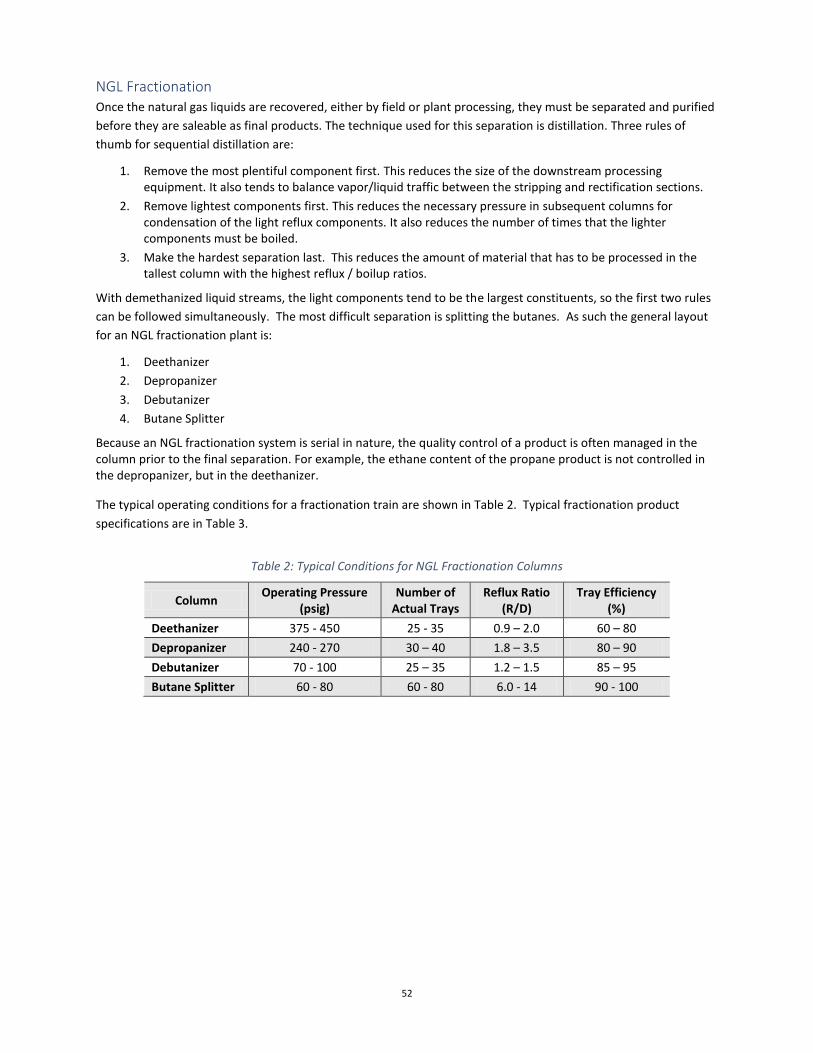
52

NGL Fractionation Once the natural gas liquids are recovered, either by field or plant processing, they must be separated and purified

before they are saleable as final products. The technique used for this separation is distillation. Three rules of

thumb for sequential distillation are:

1. Remove the most plentiful component first. This reduces the size of the downstream processing equipment. It also tends to balance vapor/liquid traffic between the stripping and rectification sections.

2. Remove lightest components first. This reduces the necessary pressure in subsequent columns for condensation of the light reflux components. It also reduces the number of times that the lighter components must be boiled.

3. Make the hardest separation last. This reduces the amount of material that has to be processed in the tallest column with the highest reflux / boilup ratios.

With demethanized liquid streams, the light components tend to be the largest constituents, so the first two rules

can be followed simultaneously. The most difficult separation is splitting the butanes. As such the general layout

for an NGL fractionation plant is:

1. Deethanizer

2. Depropanizer

3. Debutanizer

4. Butane Splitter

Because an NGL fractionation system is serial in nature, the quality control of a product is often managed in the column prior to the final separation. For example, the ethane content of the propane product is not controlled in the depropanizer, but in the deethanizer.

The typical operating conditions for a fractionation train are shown in Table 2. Typical fractionation product

specifications are in Table 3.

Table 2: Typical Conditions for NGL Fractionation Columns

Column Operating Pressure

(psig) Number of

Actual Trays Reflux Ratio

(R/D) Tray Efficiency

(%)

Deethanizer 375 - 450 25 - 35 0.9 – 2.0 60 – 80

Depropanizer 240 - 270 30 – 40 1.8 – 3.5 80 – 90

Debutanizer 70 - 100 25 – 35 1.2 – 1.5 85 – 95

Butane Splitter 60 - 80 60 - 80 6.0 - 14 90 - 100

53

Table 3: Typical Specifications for NGL Products

Analysis Unit E/P Mix Ethane Product

Propane Product

Isobutane Product

n-butane Product

Natural Gasoline

C1 LV% <1.5 <3 --- --- --- ---

C2 LV% >75, <82 >95 --- --- --- ---

C3 LV% >11.5, <25 <5 >90 <3# <0.35# ---

iC4 LV% <0.8* --- <2.5* >95 <6 ---

nC4 LV% --- --- --- <4 >94 <6#

C5+ LV% --- --- --- --- <1.5 ---

CO2 ppm wt <1000 <1000 --- --- --- ---

Sulfur ppm wt <123 <30 <100 <140 <140 ---

TVP psig --- --- <208 <70 <50 ---

RVP psi --- --- --- --- --- <14

#Includes lighter components *Includes heavier components

54

Exercise 14: Fractionation

A fractionation plant currently processes a Y-grade liquid into an E/P mix product, propane, iso and normal butane, and natural gasoline. The plant manager wants to investigate improving the product slate. Because ethane prices are low relative to propane, customers would prefer to purchase a purity ethane product. In addition, it is recognized that the plant has not been maximizing the volume of the more valuable products. Based on relative values of the products, adjust product specifications to maximize product recovery value. Start with the pre-drawn project titled “Ex14:Fractionation”, and follow the instructions below.

PROCESS SETTINGS

The Y-Grade liquid feed has the conditions and composition to the right.

The specifications for fractionation products are shown in Table 3. Assume that acid gas contamination will be handled by a downstream liquid treater.

The values (in $/bbl) of the fractionation products are:

a. Natural Gasoline (C5+) $94 b. Isobutane $59 c. Normal Butane $56 d. Propane $48 e. Ethane $11

Note the product flows before changing operation.

Modify the property table to show liquid product compositions in terms of standard liquid volume fraction. This will allow easier comparison to the product specification table.

Add the mass fraction of acid gases to the property table. Specify the units as ppm.

Add True Vapor Pressure and Reid Vapor Pressure to the property table. Add the Vapor Pressure analysis to the appropriate product streams.

The simulation is currently set up to recover an E/P Mix, which is losing market as a fractionation product. Convert the deethanizer to recover purity ethane. A possible technique for this change would be to adjust the condenser temperature to reduce the propane in the Ethane product.

Modify the deethanizer specification to maximize the amount of less valuable ethane present in the more valuable Propane product. This modification could be changing the value of the current specification, or adding a new column specification that may better reflect the product requirements.

Modify the depropanizer specifications to maximize the amount of propane present in the Butane product. Make sure the Propane product meets specification.

Modify the debutanizer specification to maximize the amount of butane in the Natural Gasoline product.

Modify the butane splitter specification to maximize the amount of n-butane in the Isobutane stream. Confirm that the specifications of both products are met.

Note the revised product flows.

PROBLEMS

What streams will require product treating? For which components?

Going through the simulation, there were product characteristics where the maximum economic value will not be achieved at the limit of the product specification. One of those values was the amount of more valuable C5+ components left in the N-Butane product. While the specification is C5+<1.5LV%, more Natural Gasoline product can be recovered at 1% C5+ in the n-Butane than at the limit of 1.5%. This parameter is available for optimization. The main tradeoff is additional Natural Gasoline recovered vs. debutanizer reboiler duty required. For a process

Inlet Conditions (“Y-Grade Feed”)

Temperature 80°F Pressure 500 psia Flow (Std.) 15000 bbl/d

Composition (“Y-Grade Feed”, mol%)

H2S 0.051 CO2 2.400 C1 0.630 C2 49.000 C3 27.000 iC4 4.150 nC4 7.600 iC5 2.200 nC5 2.140 nC6 3.800 nC7 0.600 Benzene 0.120 Toluene 0.170 Ethylbenzene 0.009 p-Xylene 0.130

55

heating cost of $4/MMBtu, calculate the incremental value of additional product recovery (Δ Product Value - Δ Reboiler Duty cost) for a change in the column specification. A value of zero indicates an economic break-even. Does this incremental value suggest that you should recover more gasoline or less?

If the price of N-Butane and Isobutane products were equal, what would be the preferred method of operating the C4 Splitter? (HINT: What type of split minimizes separation energy?)

Look at the condenser temperatures. What type of cooling system would each condenser require? In the case of the depropanizer and debutanizer, they would be more effectively managed as air-cooled heat exchangers with 120°F exit temperatures. Modify the column pressures to allow for operation with 120°F condenser temperature. (HINT: use a Phase Envelope analysis on the condenser stream to find a similar mole % Vapor condition at the new temperature) What other change would be necessary? What other operating factors should be considered in changing column pressure?

C2 Reboiler

C2 Reflux Drum

DeEthanizer

33

1

6

27

11

16

22

C3 Reboiler

C3 Condenser

DePropanizer

34

1

17

9

25

C4 Reflux Split

C4 Condenser

C4 Reboiler

DeButanizer

29

1

14

7

22

iC4 Reflux Split

iC4 Condenser

nC4 Reboiler

C4 Splitter

59

1

30

22

15

7

38

45

51

C3 Feed Cooler

C4 Reflux Pump

C2 Reflux Pump

C2 Condenser

8

7

2

4

15

14

11

1217

18

19

29

30

22

23

24

26

27

Y Grade Feed

9

10

16

Nat Gasoline

EthanePropane

21

I-Butane

N-Btuane

20

3

5

Q-1

Q-2

Q-4

Q-5

Q-6

Q-7

Q-8

Q-9

Q-3

P-2

P-1

56

Tips for Simulating a Cryo Plant The following tips have been accumulated to accurately and quickly simulate a common demethanizer plant. There

are many variations of demethanizers, so there are certainly exceptions to each tip. However, these are a good

starting point for simulation.

1. Peng-Robinson equation of state 2. Calculate C2+ liquid content of feed gas. The greater the liquid content, the lower the ethane recovery. 3. Turboexpander Efficiencies

a. Expander 75-85% adiabatic efficient b. Booster 70-80% polytropic efficient c. Shaft losses 1-2%

4. Exchanger Approach Temperatures a. Gas / Gas & Subcooler: 5°F b. Gas / Liquid: 10°F

5. Pressure Drops a. Feed Split to Expander inlet: 20-25 psi b. Column overhead to Booster suction: 23 psi c. Booster discharge to Residue Compressor suction: 10 psi d. Residue Compressor discharge to sales line: 20 psi

6. Demethanizer a. Typical number of theoretical trays 10-15. b. Approximately 0.2 psi pressure drop per theoretical tray.

7. Specify duties / temperatures of the feed stream to the demethanizer or use Qrecycle 8. Inlet feed split

a. Typically 30-35% to the reboiler. b. Will approximate the duty split between reboiler and gas/gas exchanger c. Can have multiple solutions. Lower flow to the reboiler should be higher recovery.

9. GSP a. LTS Vapor Split 20 to 35% b. Reflux 3-5 theoretical trays above expander c. Subcooler should be 2-sided exchanger d. Subcooler outlet temperature guess is 20°F below the bubble point of the inlet gas.

10. RSV a. Residue reflux 1 tray above GSP reflux b. Residue reflux split typically 10% of residue c. Residue reflux will reduce the amount of LTS vapor to subcooler d. Subcooler is a 3-sided complex exchanger e. Both refluxes will be the same temperature f. Residue recycle stream guess

i. Sales gas pressure ii. Discharge cooler temperature

iii. 10% of the molar flow of the inlet methane iv. Composition is methane

11. Evaluate the residue pressure situation. a. Sales pressure specified: Compressor and demethanizer pressure to be determined (1 degree of

freedom) b. Compressor / sales pressure specified: demethanizer pressure to be determined (0 D.O.F) c. Compressor / sales pressure / demethanizer pressure specified: Best fit of data (-1 D.O.F)

12. Molecular Sieve Dehydration a. Use a Divider block

57

References

Douglas, J. M. (1988). Conceptual Design of Chemical Processes. McGraw-Hill.

Gas Processors Suppliers Association. (2012). GPSA Engineering Data Book, 13th Edition. Tulsa, OK.

Kidnay, A. J., & Parrish, W. R. (2006). Fundamentals of natural gas processing. Taylor & Francis Group.

Lynch, J. T., & Pitman, R. N. (2000). Practical troubleshooting techniques for cryogenic gas plants. 79th Annual

Convention of the Gas Processors Association. Atlanta, GA.

Lynch, J. T., Cairo, T., Hudson, H. M., & Wilkinson, J. (2002). Unique Design Challenges in the Aux Sable NGL

recovery plant. 81st Annual Convention of the Gas Processors Association. Dallas, TX.

Lynch, J. T., Lousberg, N. B., & Pierce, M. C. (2007). How to compare cryogenic process design alternatives for a

new project. 86th Annual Convention of the Gas Processors Association. San Antonio, TX.

Ortloff Engineers. (2013, October 10). Ortloff NGL/LPG Recovery, CO2 Separation, and Sulfur Recovery

Technologies. Retrieved from http://www.uop.com/

Pitman R N, H. H. (1998). Next Generation Processes for NGL Recovery. 77th Annual Convention of the Gas

Processors Association. Dallas, TX.

Wilkinson, J. D., & Hudson, H. M. (1992). Improved NGL Recovery Designs Maximize Operating Flexibility and

Product Recovery. Meeting of the Gas Processors Association.

Wilkinson, J. H. (1993). Improving Gas Processing Profits with Retrofit Designs for Better Ethane Rejection /

Recovery. Permian Basin Regional Meeting of the Gas Processors Association, (pp. 1-21). Midland, TX.