G.A. Leonards Lecture April 26, 2019
112
Performance-Based Geotechnical Seismic Design Steve Kramer Professor of Civil and Environmental Engineering University of Washington Seattle, Washington G.A. Leonards Lecture April 26, 2019
Transcript of G.A. Leonards Lecture April 26, 2019

Performance-Based
Geotechnical Seismic Design
Steve Kramer
Professor of Civil and Environmental Engineering
University of Washington
Seattle, Washington
G.A. Leonards Lecture
April 26, 2019

Acknowledgments
Pacific Earthquake Engineering Research (PEER) Center
Washington State Department of Transportation
University of Washington
Pedro Arduino
Roy Mayfield
HyungSuk Shin
Kevin Franke
Yi-Min Huang
Sam Sideras
Mike Greenfield
Andrew Makdisi
Arduino Mayfield Shin Franke
Huang Sideras Greenfield Makdisi

Outline
Introduction
Geotechnical Design
Seismic Design
Historical Approaches
Code-Based Approaches
Performance-Based Design
Response-Level Implementation
Damage-Level Implementation
Loss-Level Implementation
Advancing Performance-Based Design
Consideration of Capacity
Load and Resistance Factor Framework
Demand and Capacity Factor Framework
Application to Pile Foundations
Summary and Conclusions

Geotechnical Design
The design process
Define performance objectives
Characterize loading
Select design approach
Preliminary design
Analysis
Are
performance
objectives
met?
Revise
design
Construction
No
Yes

The design process
Define performance objectives
Characterize loading
Select design approach
Preliminary design
Analysis
Are
performance
objectives
met?
Revise
design
Construction
No
Yes
Geotechnical Design

The design process
Define performance objectives
Characterize loading
Select design approach
Preliminary design
Analysis
Are
performance
objectives
met?
Revise
design
Construction
No
Yes
What do we mean by “performance?”
Demand exceeding capacity (force, stress-based)?
Factor of safety
Predictability of demands?
Predictability of capacities?
Minimum allowable FS value?
Geotechnical Design

The design process
Define performance objectives
Characterize loading
Select design approach
Preliminary design
Analysis
Are
performance
objectives
met?
Revise
design
Construction
No
Yes
What do we mean by “performance?”
Demand exceeding capacity (force, stress-based)?
Excessive deformations?
Vertical, horizontal, tilting, rotation
Predictability of deformation demands?
Predictability of deformation capacities?
Maximum allowable deformations?
Geotechnical Design

The design process
Define performance objectives
Characterize loading
Select design approach
Preliminary design
Analysis
Are
performance
objectives
met?
Revise
design
Construction
No
Yes
What do we mean by “performance?”
Demand exceeding capacity (force, stress-based)?
Excessive deformations?
Excessive physical damage?
Cracking, spalling, hinging, etc.?
Catastrophic damage (e.g., collapse)?
Characterization of physical damage
Predictability of physical damage?
Geotechnical Design

The design process
Define performance objectives
Characterize loading
Select design approach
Preliminary design
Analysis
Are
performance
objectives
met?
Revise
design
Construction
No
Yes
What do we mean by “performance?”
Demand exceeding capacity (force, stress-based)?
Excessive deformations?
Excessive physical damage?
Excessive losses?
High repair costs
Extended loss of service (downtime)
Casualties
Geotechnical Design

Historical Approaches to Seismic Design
Pseudo-Static
Retaining walls
Mononobe and
Matsuo (1926)
Okabe (1926)

Pseudo-Static
Retaining walls
Okabe (1926)
Mononobe and
Matsuo (1929)
Historical Approaches to Seismic Design
Force-based

Pseudo-Static
Retaining walls
Slopes
Historical Approaches to Seismic Design
Force-based

Pseudo-Static
Retaining walls
Slopes
Foundations
Historical Approaches to Seismic Design
Force-based
Results expressed in
terms of factor of safety

Displacement-based
Newmark analysis
Historical Approaches to Seismic Design
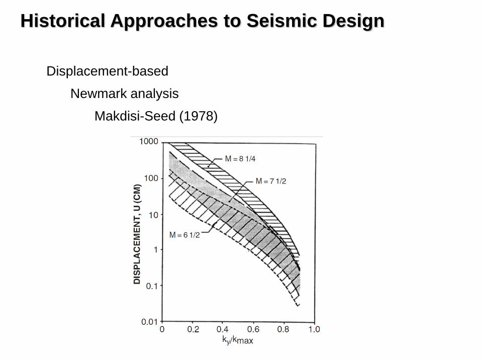
Displacement-based
Newmark analysis
Makdisi-Seed (1978)
Historical Approaches to Seismic Design

Displacement-based
Newmark analysis
Makdisi-Seed (1978)
Travasarou and Bray (2007)
Historical Approaches to Seismic Design

Displacement-based
Newmark analysis
Makdisi-Seed (1978)
Bray and Travasarou (2007)
Rathje and Saygili (2009)
Historical Approaches to Seismic Design

Displacement-based
Newmark analysis
Makdisi-Seed (1978)
Bray and Travasarou (2007)
Rathje and Saygili (2009)
Stress-deformation analysis
Slopes
Historical Approaches to Seismic Design

Displacement-based
Newmark analysis
Makdisi-Seed (1978)
Bray and Travasarou (2007)
Rathje and Saygili (2009)
Stress-deformation analysis
Shallow
foundations
Historical Approaches to Seismic Design

Displacement-based
Newmark analysis
Makdisi-Seed (1978)
Bray and Travasarou (2007)
Rathje and Saygili (2009)
Stress-deformation analysis
Deep
foundations
Historical Approaches to Seismic Design

Displacement-based
Newmark analysis
Makdisi-Seed (1978)
Bray and Travasarou (2007)
Rathje and Saygili (2009)
Stress-deformation analysis
Macro-elements
H
V
M M
H
V
Pecker (2004)
Historical Approaches to Seismic Design

Displacement-based
Newmark analysis
Makdisi-Seed (1978)
Bray and Travasarou (2007)
Rathje and Saygili (2009)
Stress-deformation analysis
Macro-elements
After Hutchinson et
al. (2002)
Correia et al.
(2012)
Historical Approaches to Seismic Design

Code-Based Seismic Design
• a minor level of shaking without damage (non-structural or
structural),
• a moderate level of shaking without structural damage (but
possibly with some non-structural damage), and
• a strong level of shaking without collapse (but possibly with
both non-structural and structural damage).
Early building codes – first edition of SEAOC Blue Book:
Intended that structure be able to resist:
Multiple levels of seismic loading
Multiple performance objectives
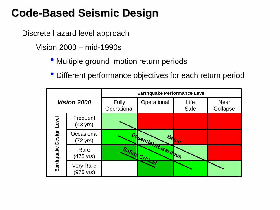
Discrete hazard level approach
Vision 2000 – mid-1990s
• Multiple ground motion return periods
• Different performance objectives for each return period
Ea
rth
qu
ak
e D
es
ign
Leve
l
Vision 2000
Earthquake Performance Level
Fully
Operational
Operational Life
Safe
Near
Collapse
Frequent
(43 yrs)
Occasional
(72 yrs)
Rare
(475 yrs)
Very Rare
(975 yrs)
Code-Based Seismic Design

Earthquake Losses
Process leading to losses
Ground
motion Loss
Physical
damage
System
response
PGA,
Sa(To), Ia,
CAV
dh, dv, f Crack
width,
spacing
Deaths,
dollars,
downtime

Deaths,
Injuries,
Repair cost,
Downtime,
etc.
Concrete
spalling,
Column
cracking,
etc.
Losses
Interstory drift,
Plastic
rotation,
Ground
deformation,
etc.
Physical
Damage
Peak
acceleration,
Spectral
acceleration,
Arias intensity,
etc.
System
Response
Ground
motion
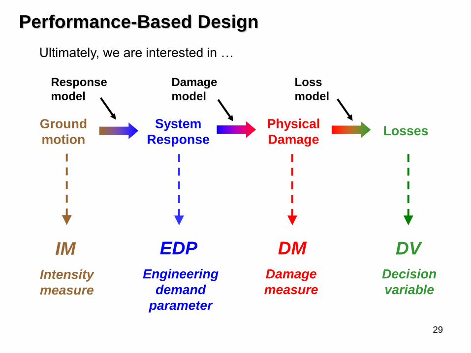
Ultimately, we are interested in …
Performance-Based Design
Response
model
Damage
model
Loss
model
Losses Physical
Damage
System
Response
Ground
motion
Ultimately, we are interested in …
Performance-Based Design
Response
model
Damage
model
Loss
model
29
IM
Intensity
measure
EDP
Engineering
demand
parameter
DM
Damage
measure
DV
Decision
variable

Losses Physical
Damage
System
Response
Ground
motion
Ultimately, we are interested in …
Performance-Based Design
Response
model
Damage
model
Loss
model
30
IM
Intensity
measure
EDP
Engineering
demand
parameter
DM
Damage
measure
DV
Decision
variable
Response given
ground motion
Damage given
response
Loss given
damage
EDP | IM DM | EDP DV | DM
All are uncertain !!!

Performance-Based Design
31
Uncertainty exists – can’t ignore it
• Uncertainty in ground motions varies from location to location
• Uncertainty in response varies from site to site
• Uncertainty in damage varies from structure to structure
• Uncertainty in loss varies with location (material costs, labor
costs, …) and time (inflation, interest rates, etc.)
Ignoring uncertainty, or assuming it is uniform, leads to:

Performance-Based Design
32
Uncertainty exists – can’t ignore it
• Uncertainty in ground motions varies from location to location
• Uncertainty in response varies from site to site
• Uncertainty in damage varies from structure to structure
• Uncertainty in loss varies with location (material costs, labor
costs, …) and time (inflation, interest rates, tweets, …)
Ignoring uncertainty, or assuming it is uniform, leads to:
• Inaccurate performance predictions

Performance-Based Design
33
Uncertainty exists – can’t ignore it
• Uncertainty in ground motions varies from location to location
• Uncertainty in response varies from site to site
• Uncertainty in damage varies from structure to structure
• Uncertainty in loss varies with location (material costs, labor
costs, …) and time (inflation, interest rates, tweets, …)
Ignoring uncertainty, or assuming it is uniform, leads to:
• Inaccurate performance predictions
• Inconsistent levels of safety from one project to another

Performance-Based Design
34
Uncertainty exists – can’t ignore it
• Uncertainty in ground motions varies from location to location
• Uncertainty in response varies from site to site
• Uncertainty in damage varies from structure to structure
• Uncertainty in loss varies with location (material costs, labor
costs, …) and time (inflation, interest rates, tweets, …)
Ignoring uncertainty, or assuming it is uniform, leads to:
• Inaccurate performance predictions
• Inconsistent levels of safety from one project to another
• Inefficient use of resources for seismic retrofit/design

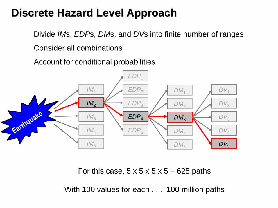
Divide IMs, EDPs, DMs, and DVs into finite number of ranges
Consider all combinations
Account for conditional probabilities
Discrete Hazard Level Approach
IM1
IM2
IM3
IM4
IM5

Discrete Hazard Level Approach
EDP1
EDP2
EDP3
EDP4
EDP5
IM1
IM2
IM3
IM4
IM5
Divide IMs, EDPs, DMs, and DVs into finite number of ranges
Consider all combinations
Account for conditional probabilities

Discrete Hazard Level Approach
EDP1
EDP2
EDP3
EDP4
EDP5
IM1
IM2
IM3
IM4
IM5
DM1
DM2
DM3
DM4
DM5
Divide IMs, EDPs, DMs, and DVs into finite number of ranges
Consider all combinations
Account for conditional probabilities

Discrete Hazard Level Approach
EDP1
EDP2
EDP3
EDP4
EDP5
IM1
IM2
IM3
IM4
IM5
DM1
DM2
DM3
DM4
DM5
DV1
DV2
DV3
DV4
DV5
Divide IMs, EDPs, DMs, and DVs into finite number of ranges
Consider all combinations
Account for conditional probabilities

Discrete Hazard Level Approach
EDP1
EDP2
EDP3
EDP4
EDP5
IM1
IM2
IM3
IM4
IM5
DM1
DM2
DM3
DM4
DM5
DV1
DV2
DV3
DV4
DV5
Divide IMs, EDPs, DMs, and DVs into finite number of ranges
Consider all combinations
Account for conditional probabilities

Discrete Hazard Level Approach
EDP1
EDP2
EDP3
EDP4
EDP5
IM1
IM2
IM3
IM4
IM5
DM1
DM2
DM3
DM4
DM5
DV1
DV2
DV3
DV4
DV5
DV2-4-3-5 = DV5
DV = S DVi-j-k-l Summing over all paths
Divide IMs, EDPs, DMs, and DVs into finite number of ranges
Consider all combinations
Account for conditional probabilities
P[IM2|eq] P[EDP4|IM2] P[DM3|EDP4] P[DV5|DM3]
Discrete Hazard Level Approach
EDP1
EDP2
EDP3
EDP4
EDP5
IM1
IM2
IM3
IM4
IM5
DM1
DM2
DM3
DM4
DM5
DV1
DV2
DV3
DV4
DV5
Divide IMs, EDPs, DMs, and DVs into finite number of ranges
Consider all combinations
Account for conditional probabilities
For this case, 5 x 5 x 5 x 5 = 625 paths
With 100 values for each . . . 100 million paths

Covers entire range of hazard (ground motion) levels
Accounts for uncertainty in parameters, relationships
PEER framework
)()|()|()|()( IMIMEDPEDPDMDMDVDV ddGdGG
Integral Hazard Level Approach

Loss
model
Loss curve
– Cost vs
Cost
Seismic
hazard
curve – Sa
vs Sa
Fragility curve
– interstory
drift given Sa
Fragility curve
– crack width
given
interstory drift
Fragility curve –
repair cost given
crack width
PSHA Response
model
Damage
model
Covers entire range of hazard (ground motion) levels
Accounts for uncertainty in parameters, relationships
PEER framework
)()|()|()|()( IMIMEDPEDPDMDMDVDV ddGdGG
Integral Hazard Level Approach
$2.7M $5.8M

Risk curve
– Cost vs
Cost
Seismic
hazard
curve – Sa
vs Sa
Fragility curve
– interstory
drift given Sa
Fragility curve
– crack width
given
interstory drift
Fragility curve –
repair cost given
crack width
PSHA Response
model
Damage
model
Cost
model
Covers entire range of hazard (ground motion) levels
Accounts for uncertainty in parameters, relationships
PEER framework
)()|()|()|()( IMIMEDPEDPDMDMDVDV ddGdGG
PEER Performance-Based Framework
Alternative
design
$1.6M $3.9M

Modular – response, damage, loss components
PEER Performance-Based Framework
IM
log
IM
DM
log
D
M
EDP
log
E
DP
DV
log
DV
PGA Settlement
Floor slab
cracking Repair
cost

Modular – response, damage, loss components
PEER Performance-Based Framework
IM
log
IM
DM
log
D
M
EDP
log
E
DP
DV
log
D
V
PGA Settlement
Floor slab
cracking Repair
cost
Includes - all earthquake magnitudes
- uncertainty in ground motion
- uncertainty in response given ground motion
- uncertainty in damage given response
- uncertainty in loss given damage
All levels of shaking are
cosidered and accounted for,
not just shaking at one return
period.
- all source-to-site distances

Modular – response, damage, loss components
PEER Performance-Based Framework
IM
log
IM
DM
log
D
M
EDP
log
E
DP
DV
log
D
V
PGA Settlement
Floor slab
cracking Repair
cost
Includes - all earthquake magnitudes
- uncertainty in ground motion
- uncertainty in response given ground motion
- uncertainty in damage given response
- uncertainty in loss given damage
Response, damage, and loss
are all explicitly computed –
with explicit consideration of
uncertainty in each
- all source-to-site distances
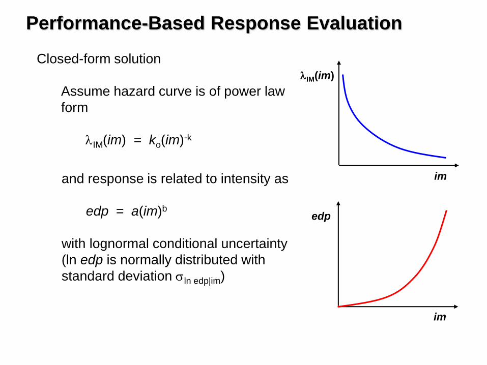
Closed-form solution
Assume hazard curve is of power law
form
IM(im) = ko(im)-k
Performance-Based Response Evaluation
IM(im)
im
edp
im
and response is related to intensity as
edp = a(im)b
with lognormal conditional uncertainty
(ln edp is normally distributed with
standard deviation sln edp|im)

Closed-form solution
Then median EDP hazard curve can be expressed in closed form as
IM(im)
im
edp
im
EDP(edp)
edp
s 2|ln2
2/1
2exp)( imedp
kb
oEDPb
k
a
edpkedp
Performance-Based Response Evaluation

Closed-form solution
Then median EDP hazard curve can be expressed in closed form as
EDP(edp)
edp
Based on median
IM and EDP-IM
relationship
EDP “amplifier” based
on uncertainty in
EDP|IM relationship
s 2|ln2
2/1
2exp)( imedp
kb
oEDPb
k
a
edpkedp
Performance-Based Response Evaluation

Closed-form solution
Example: Slope displacement
Performance-Based Response Evaluation
Combining, with different levels of response model uncertainty
…

Closed-form solution
Example: Slope displacement
Performance-Based Response Evaluation
Uncertainty in response
prediction accounts for half

Closed-form solution
Extending to DM and DV, with same assumptions, gives
Performance-Based Loss Evaluation
dv
DV(dv) Median relationship (no uncertainty)
222222
222
2
//1
/1
02
exp11
)(LDR
bkd
f
DV ffdfdb
k
e
dv
cakdv
Median relationships Uncertainty amplifier
Response
model
Damage
model Loss
model
With response model uncertainty
Response and damage model uncertainties
Response, damage, and loss model
uncertainties
Losses
1/TR

Characterization of loading
Select IMs – important considerations include:
Efficiency – how well does IM predict response?
Dis
pla
cem
ent
(cm
)
PGA (g) Arias intensity (m/s) PGV2 (cm/s)2
Travasarou et al. (2003)
Implementation of Performance-Based Design
Permanent displacement of shallow slides

Characterization of loading
Select IMs
Efficiency – how well does IM predict response?
Sufficiency – how completely does IM predict response?
Implementation of Performance-Based Design
Systematic trend in pore
pressure residuals w/r/t Mw
Magnitude scaling factor
Kramer and Mitchell (2003)
Deviations from mean excess pore pressure ratio
correlation to PGA
Weak trend w/r/t R
ru over-
predicted
ru under-
predicted

Characterization of loading
Select IMs
Efficiency – how well does IM predict response?
Sufficiency – how completely does IM predict response?
Predictability – how well can we predict IM?
Intensity Measure, IM Standard error, sln IM Reference
PGA 0.53 – 0.55 Campbell and Bozorgnia, 2008
PGV 0.53 – 0.56 Campbell and Bozorgnia, 2008
Sa (0.2 sec) 0.59 – 0.61 Campbell and Bozorgnia, 2008
Sa (1.0 sec) 0.62 – 0.66 Campbell and Bozorgnia, 2008
Arias intensity, Ia 1.0 – 1.3 Travasarou et al. (2003)
CAV 0.40 – 0.44 Campbell and Bozorgnia, 2010
Implementation of Performance-Based Design

Characterization of loading
Select IMs
Efficiency – how well does IM predict response?
Sufficiency – how completely does IM predict response?
Predictability – how well can we predict IM?
Good predictability
Poor predictability
Implementation of Performance-Based Design

Characterization of loading
Select IMs
Efficiency – how well does IM predict response?
Sufficiency – how completely does IM predict response?
Predictability – how well can we predict IM?
Example:
Implementation of Performance-Based Design

EDP Hazard Curves
Worse predictability, worse efficiency
Better predictability, better efficiency
Worse predictability, better efficiency
Better predictability, worse efficiency
Implementation of Performance-Based Design
Characterization of loading
Select IMs
Efficiency – how well does IM predict response?
Sufficiency – how completely does IM predict response?
Predictability – how well can we predict IM?
Example:
Typical predictability, typical efficiency

50-yr exceedance probabilities
Implementation of Performance-Based Design
Characterization of loading
Select IMs
Efficiency – how well does IM predict response?
Sufficiency – how completely does IM predict response?
Predictability – how well can we predict IM?
Example:
Predictability and efficiency both
affect response for a given
return period
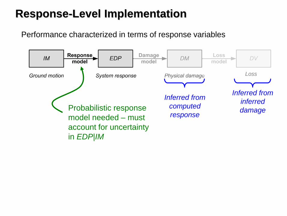
Performance characterized in terms of response variables
Response-Level Implementation
Inferred from
computed
response
Inferred from
inferred
damage
Loss
Probabilistic response
model needed – must
account for uncertainty
in EDP|IM

Performance characterized in terms of response variables
Response-Level Implementation
Site response
)(]|[)(0
rIMrsSsIM imdimimIMPimRS
0
)(]|[)( rIMr
r
s
sIM imdimim
imAFPim
RS
Rock
hazard
curve
Soil
hazard
curve
Uncertainty in
amplification
behavior
Integrating over
all rock motion
levels
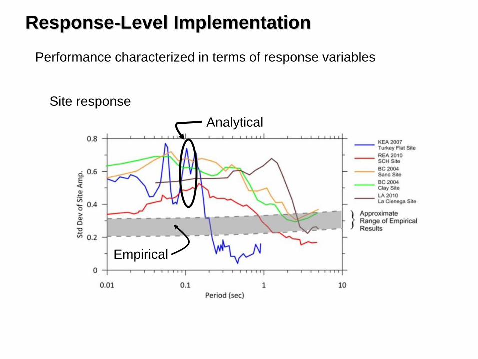
Performance characterized in terms of response variables
Response-Level Implementation
Site response
Empirical
Analytical

Performance characterized in terms of response variables
Response-Level Implementation
6 m
Distributions of M
at all hazard levels
considered
Liquefaction (Kramer and Mayfield, 2007)
FSL hazard curves
TR = 5000 yrs
TR = 50 yrs

Lateral Spreading – Franke and Kramer (2014)
Reference soil profile
(N1)60
Displacement hazard curves
Response-Level Implementation

Post-liquefaction settlement (Kramer and Huang, 2010)
Performance characterized in terms of response variables
Response-Level Implementation
Assuming soil is susceptible,
liquefaction is triggered, and
neglecting maximum
volumetric strain
Considering maximum
volumetric strain
Considering
susceptibility
Hypothetical site in Seattle, Washington
Settlement hazard curves
Considering
triggering
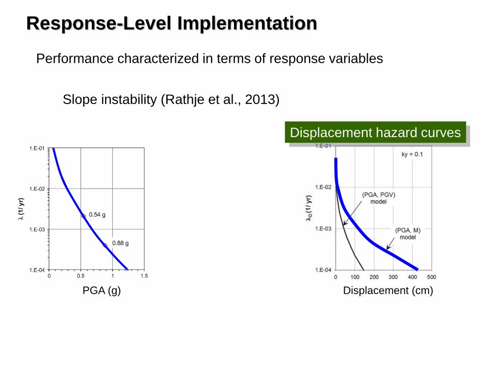
Slope instability (Rathje et al., 2013)
Performance characterized in terms of response variables
Response-Level Implementation
PGA (g)
Displacement hazard curves
Displacement (cm)

Slope instability (Rathje et al., 2013)
Performance characterized in terms of response variables
Response-Level Implementation
Displacement hazard curves
PGA (g) Displacement (cm)
Vector IM cuts
displacement in half
PGV
(cm/sec)

Uncertainties from different sliding block models
Performance characterized in terms of response variables
Response-Level Implementation
Flexible sliding
mass model
PGA and Mw
PGA and PGV

Performance characterized in terms of damage measures
Damage-Level Implementation
Requires:
Characterization of allowable levels of physical damage
Damage model
How much settlement is required to crack a slab?
How much lateral displacement is required to
produce hinging in a concrete pile? in a steel pile?
Inferred from
damage

Continuous DM scales
Fragility curve approach
Some damage states (e.g., collapse) are binary
Insufficient data available for others
Discrete DM scales
Damage probability matrix approach
Performance characterized in terms of damage measures
Damage-Level Implementation
Damage
State, DM Description
EDP interval
edp1 edp2 edp3 edp4 edp5
dm1 Negligible X11 X12 X13 X14 X15
dm2 Slight X21 X22 X23 X24 X25
dm3 Moderate X31 X32 X33 X34 X35
dm4 Severe X41 X42 X43 X44 X45
dm5 Catastrophic X51 X52 X53 X54 X55
Probability that response
in EDP interval 2
produces severe damage

Performance characterized in terms of damage measures
Damage-Level Implementation
N = None
S = Small
M = Moderate
L = Large
C = Collapse
Ledezma and
Bray, 2010
Fragility curve approach
Continuous DM scales difficult to quantify
Some damage states (e.g., collapse) are binary
Insufficient data available for others
Damage probability matrix approach
Pile-supported
bridge founded on
liquefiable soils

Performance characterized in terms of damage measures
Damage-Level Implementation
Ledezma and
Bray, 2010
Fragility curve approach
Continuous DM scales difficult to quantify
Some damage states (e.g., collapse) are binary
Insufficient data available for others
Damage probability matrix approach

Performance characterized in terms of damage measures
Damage-Level Implementation
Ledezma and
Bray, 2010
Fragility curve approach
Continuous DM scales difficult to quantify
Some damage states (e.g., collapse) are binary
Insufficient data available for others
Damage probability matrix approach

Example: Caisson quay wall (Iai, 2008)
Life cycle cost as decision variable, DV
Loss-Level Implementation
Performance characterized in terms of decision variables
Construction Costs
Indirect Losses
Direct Losses
Life-Cycle
Costs
Options
A: Foundation compaction only
B: Foundation cementation
C: Foundation and backfill compaction (1.8 m spacing)
D: Foundation & backfill compaction (1.6 m spacing)
E: Foundation compaction & structural modification
Options:
A: Foundation compaction only
B: Foundation cementation
C: Foundation and backfill compaction
(1.8 m spacing)
D: Foundation and backfill compaction
(1.6 m spacing)
E: Foundation compaction and
structural modification

Example: Expressway embankment widening (Towhata, 2008)
Life cycle cost as decision variable, DV
Loss-Level Implementation
Performance characterized in terms of decision variables
5 m widening with
deep mixing

Fragility curve approach – Kramer et al. (2009)
Pile-supported bridge on liquefiable soils
Performance characterized in terms of decision variables
Loss-Level Implementation

Loss-Level Implementation
1
10-2
10-4
10-6
Repair cost ratio, RCR
0.0 0.2 0.4 0.6 0.8 1.0 Me
an
an
nu
al ra
te o
f e
xce
ed
an
ce
1,000 yrs
100 yrs
Return
period
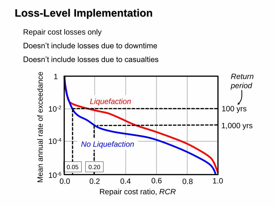
Repair cost losses only
Doesn’t include losses due to downtime
Doesn’t include losses due to casualties
0.16 0.47
Loss-Level Implementation
1
10-2
10-4
10-6
Repair cost ratio, RCR
0.0 0.2 0.4 0.6 0.8 1.0 Me
an
an
nu
al ra
te o
f e
xce
ed
an
ce
100 yrs
1,000 yrs
Return
period
Repair cost losses only
Doesn’t include losses due to downtime
Doesn’t include losses due to casualties
0.05 0.20
Liquefaction
No Liquefaction

Impacts on bridge structure
PBEE framework allows deaggregation of costs
'Temporary
support
(abutment)'
'Furnish steel
pipe pile'
'Joint seal
assembly'
'Column steel
casing'
'Structure
excavation'
'Aggregate base
(approach slab)'
'Elastomeric
bearings'
'Other' 'Structure
backfill'
'Bar reinforcing
steel (footing,
retaining wall)'
Loss-Level Implementation
475-yr losses

Advancing Performance-Based Design
Improved Characterization of Capacity
How should we characterize physical damage?
How much ground movement can structures tolerate?
Bird et al. (2005; 2006)
Analyses of RC frame buildings subjected to ground deformation
Four damage states:
None to slight – linear elastic response, flexural or shear-type
hairline cracks (<1 mm) in some members, no yielding in any
critical section
Moderate – member flexural strengths achieved, limited ductility
developed, crack widths reach 1 mm, initiation of concrete spalling
Extensive – significant repair required to building, wide flexural or
shear cracks, buckling of longitudinal reinforcement may occur
Complete – repair of building not feasible either physically or
economically, demolition after earthquake required, could be due
to shear failure of vertical elements or excess displacement
LS1
LS2
LS3

Advancing Performance-Based Design
Improved Characterization of Capacity
How should we characterize physical damage
How much ground movement can structures tolerate?
Bird et al. (2005)
Analyses of structures subjected to ground deformation
Horizontal Vertical
High uncertainty
Rational, quantified fragility curves for R/C frame buildings

Advancing Performance-Based Design
Improved Characterization of Capacity
Effects of uncertainty in capacity
Response hazard curve
i
N
i
ijjEDP imIMPimIMedpEDPPedpIM
1
|)(
s 2|ln2
2/
|2
1exp)( IMEDP
bk
oCEDPb
k
a
ckc
0
| )()()( dccfcedp CCEDPEDP
ss 2
ln2
2
2|ln2
2
2
1exp
2
1exp)()( ln
CIMEDPIMEDPb
k
b
kimc C
Let C = capacity (response corresponding to given damage state)
Integrating over distribution of capacity
Assuming lognormal capacity distribution
Capacity
uncertainty
amplifier

Advancing Performance-Based Design
Improved Characterization of Capacity
Effects of uncertainty in capacity
Accurate characterization of uncertainty in capacity
nearly as important as uncertainty in response
Increasing
uncertainty in
capacity
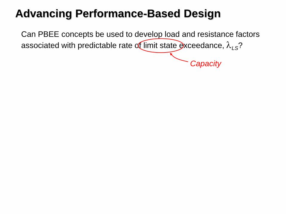
Can PBEE concepts be used to develop load and resistance factors
associated with predictable rate of limit state exceedance, LS?
Capacity
Advancing Performance-Based Design

Can PBEE concepts be used to develop load and resistance factors
associated with predictable rate of limit state exceedance, LS?
Let LM = load measure = aIMb
lm
LM (lm)
bk
LMa
lmklm
/
0)(
2
2
2/
02
exp)(L
bk
LMb
k
a
lmklm
No uncertainty
Uncertainty
in loading
Capacity
Advancing Performance-Based Design

Can PBEE concepts be used to develop load and resistance factors
associated with predictable rate of limit state exceedance, LS?
Let LM = load measure = aIMb
lm
LM (lm)
bk
LMa
lmklm
/
0)(
2
2
2/
02
exp)(L
bk
LMb
k
a
lmklm
22
2
2/
2
1exp
CL
bk
oLMb
k
a
lmk
No uncertainty
Uncertainty
in loading
Uncertainty in
loading and capacity
Capacity
Advancing Performance-Based Design

Can PBEE concepts be used to develop load and resistance factors
associated with predictable rate of limit state exceedance, LS?
Let LM = load measure
lm
LM (lm)
LMLC LML LM0
Solving previous equations for LM,
kb
LM
kaLM
/
0
0
2
/
0 2exp L
kb
LML
b
k
kaLM
22
/
0 2exp CL
kb
LMLC
b
k
kaLM
LS
Advancing Performance-Based Design

Can PBEE concepts be used to develop load and resistance factors
associated with predictable rate of limit state exceedance, LS?
Let LM = load measure
lm
LM (lm)
LS
LMLC LML LM0
LMLC can be interpreted as median capacity
that will be exceeded every TR years, on
average, and LM0 as the median load. Then
this will occur when
0
ˆˆLM
LML
LM
LMC L
LC
L
LC ˆˆ for
L
LCLLC
LM
LM
LM
LMLMLM
0
0
L C
Advancing Performance-Based Design

Can PBEE concepts be used to develop load and resistance factors
associated with predictable rate of limit state exceedance, LS?
Let LM = load measure
lm
LM (lm)
LS
LMLC LML LM0
0LM
LM LLC
L
LM
LMf
So,
Substituting closed-form LM expressions,
2
2
1exp
Lb
k
f
2
2
1exp
Cb
k
Load factor
Resistance
factor
Uncertainty
in loading
Uncertainty
in capacity
Advancing Performance-Based Design

Extension to foundation displacements
Let LM = load measure, EDP = response measure
Note that LM = {Q, Vx, Vy, Mx, My}
EDP = {w, u, v, qx, qy}
Q
Vx
Vy
Mx
My
w
u
v
qy qx
Loads
(LMs)
Deformations
(EDPs)
Application to Foundation Design

Extension to foundation displacements
Let LM = load measure, EDP = response measure
Note that LM = {Q, Vx, Vy, Mx, My}
EDP = {w, u, v, qx, qy}
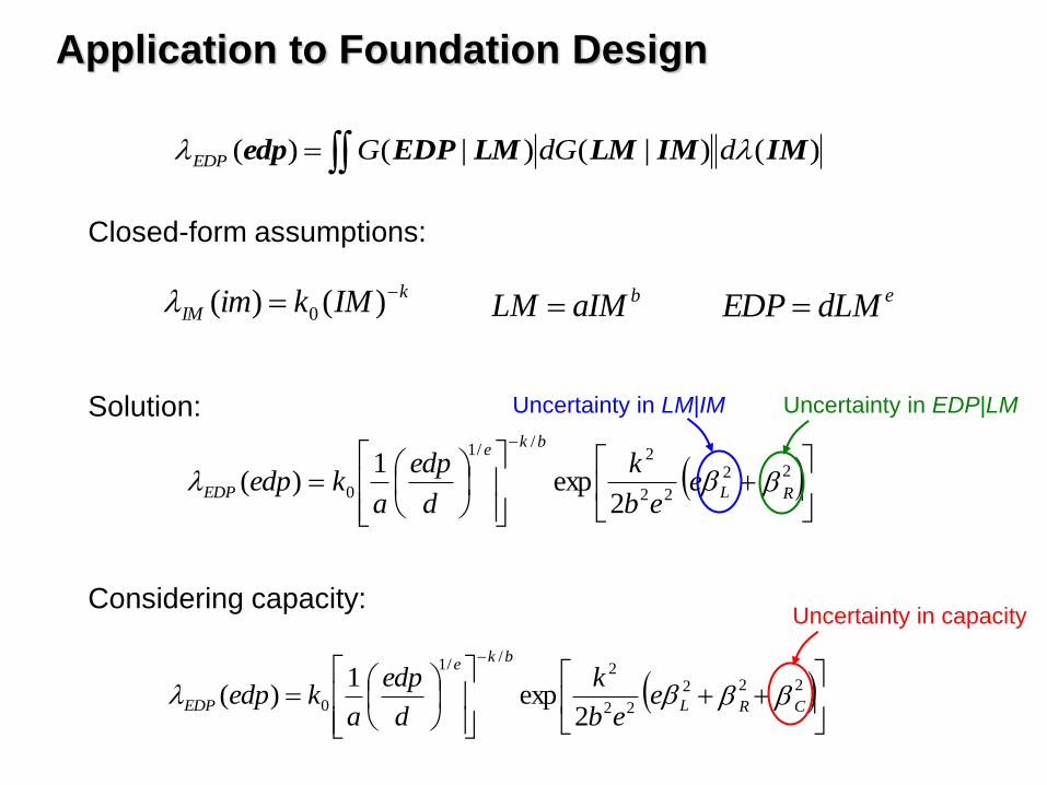
)()|()|()( IMIMLMLMEDPedp ddGGEDP
Closed-form assumptions:
k
IM IMkim )()( 0 baIMLM edLMEDP
Loads and moments
Displacements
and rotations
Application to Foundation Design
)()|()|()( IMIMLMLMEDPedp ddGGEDP
Closed-form assumptions:
k
IM IMkim )()( 0 baIMLM edLMEDP
22
22
2/
/1
02
exp1
)(RL
bke
EDP eeb
k
d
edp
akedp
Solution:
222
22
2/
/1
02
exp1
)(CRL
bke
EDP eeb
k
d
edp
akedp
Considering capacity:
Uncertainty in LM|IM Uncertainty in EDP|LM
Uncertainty in capacity
Application to Foundation Design
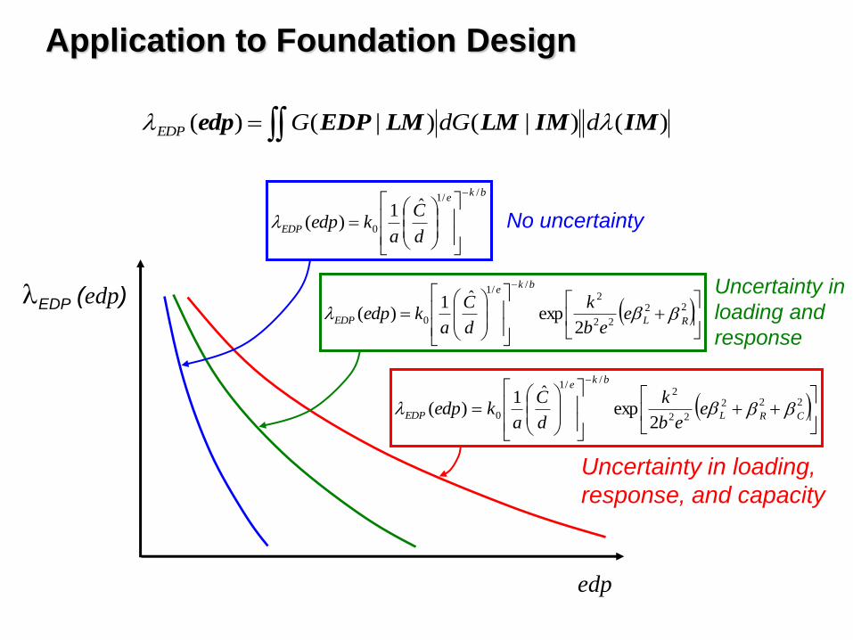
)()|()|()( IMIMLMLMEDPedp ddGGEDP
edp
No uncertainty
Uncertainty in
loading and
response
Uncertainty in loading,
response, and capacity
bke
EDPd
C
akedp
//1
0
ˆ1)(
22
22
2/
/1
02
expˆ1
)(RL
bke
EDP eeb
k
d
C
akedp
222
22
2/
/1
02
expˆ1
)(CRL
bke
EDP eeb
k
d
C
akedp
EDP (edp)
Application to Foundation Design

)()|()|()( IMIMLMLMEDPedp ddGGEDP
edp
EDP (edp)
LS
EDPLRC EDPLR EDP0
Solving previous equations for EDP,
22
/
/
0 2exp
RL
kbe
bk
EDPLR e
be
k
akdEDP
222
/
/
0 2exp
CRL
kbe
bk
EDPLRC e
be
k
akdEDP
kbe
bk
EDP
akdEDP
/
/
0
0
Application to Foundation Design

)()|()|()( IMIMLMLMEDPedp ddGGEDP
lm
LM (lm)
LS
EDPLRC EDPLR EDP0
EDPLRC can be interpreted as median displacement
capacity that will be exceeded every TR years, on average,
and EDP0 as the median displacement demand. Then
this will occur when
0
ˆˆEDP
EDPD
EDP
EDPC LR
LRC
LR
LDFCCF ˆˆ or
LR
LRCLRLRC
EDP
EDP
EDP
EDPEDPEDP
0
0
Application to Foundation Design

)()|()|()( IMIMLMLMEDPedp ddGGEDP
0EDP
EDPDF LR
LRC
LR
EDP
EDPCF
So,
Substituting closed-form LM expressions,
lm
LM (lm)
LS
EDPLRC EDPLR EDP0
)(
2
1exp
222 RL
ebe
kDF
2
2
1exp
Cbe
kCF
Demand factor
Capacity factor
Application to Foundation Design
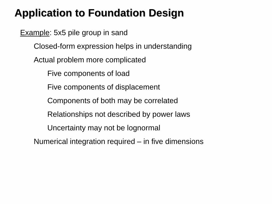
Example: 5x5 pile group in sand
Closed-form expression helps in understanding
Actual problem more complicated
Five components of load
Five components of displacement
Components of both may be correlated
Relationships not described by power laws
Uncertainty may not be lognormal
Numerical integration required – in five dimensions
Application to Foundation Design

LM|IM
Computational approach: Decoupled analyses
Application to Foundation Design

LM|IM
p-y t-z
Q-z
Computational approach: Decoupled analyses
Application to Foundation Design

LM|IM
p-y t-z
Q-z
EDP|LM
Computational approach: Decoupled analyses
Application to Foundation Design
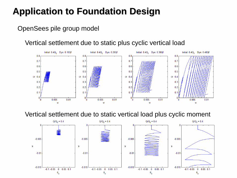
OpenSees pile group model
Vertical settlement due to static plus cyclic vertical load
Vertical settlement due to static vertical load plus cyclic moment
Application to Foundation Design

OpenSees pile group model
Analyzed multiple cases:
3 x 3
5 x 5
7 x 7
3 x 5
3 x 7 groups
Sand profile
Clay profile
Linear structure, To = 0.5 sec
Linear structure, To = 1.0 sec
Nonlinear structure, To = 0.5 sec
Nonlinear structure, To = 1.0 sec
Fault normal Fault parallel Vertical
50 three-component motions
Application to Foundation Design

OpenSees pile group model
Analyzed multiple cases:
)ln(796.0320.0990.0ln364.0191.0ln ynxnynxnnn MMVVQu
749.0ln nus
Normalized
displacement vs.
normalized load
Application to Foundation Design
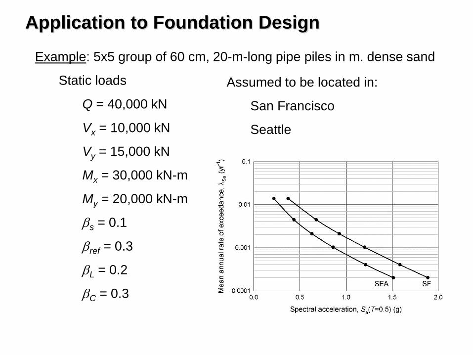
Example: 5x5 group of 60 cm, 20-m-long pipe piles in m. dense sand
Static loads
Q = 40,000 kN
Vx = 10,000 kN
Vy = 15,000 kN
Mx = 30,000 kN-m
My = 20,000 kN-m
s = 0.1
ref = 0.3
L = 0.2
C = 0.3
Assumed to be located in:
San Francisco
Seattle
Application to Foundation Design

Example: 5x5 group of 60 cm, 20-m-long pipe piles in m. dense sand
San Francisco
Seattle
Application to Foundation Design
Example: 5x5 group of 60 cm, 20-m-long pipe piles in m. dense sand
San Francisco
Seattle
Application to Foundation Design

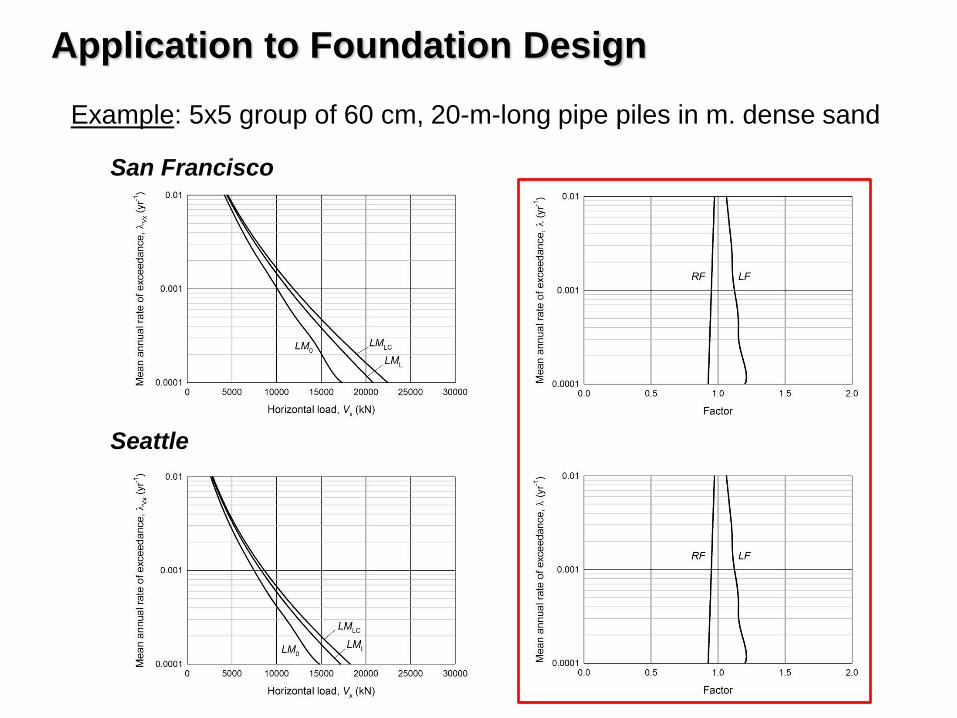
Example: 5x5 group of 60 cm, 20-m-long pipe piles in m. dense sand
San Francisco
Seattle
Uncertainties in forces are relatively low
LM hazard curves are close to each other
Load and resistance factors vary with TR
Load and resistance factors close to 1.0
Application to Foundation Design

Example: 5x5 group of 60 cm, 20-m-long pipe piles in m. dense sand
San Francisco
Seattle
Uncertainties in displacements are high
EDP hazard curves are far from each other
Load and resistance factors not close to 1.0
Application to Foundation Design

•Seismic design has always considered performance, but not always
in rigorous manner
•Performance can be characterized in different ways – response,
damage, loss
• It is important to define performance objectives in clear, quantitative
way
•Design for specified performance level requires consideration of
uncertainties
•For a given return period, response, damage, and loss all increase
with increasing uncertainty
•Geotechnical engineers are able to reduce expected losses by
reducing uncertainty through more extensive subsurface
investigation, improved field and laboratory testing, and more
rigorous analyses
Summary and Conclusions

•Application of performance-based concepts has increased – usually
implemented in terms of response measures (displacement, rotation,
curvature, etc.)
•Performance-based concepts can be implemented for such
structures in LRFD-type format
•Force-based load and resistance factors reflect relatively low
uncertainty in ability to predict forces
•Displacement-based demand and capacity factors reflect high
uncertainty in displacements
•Performance-based earthquake engineering offers a framework for
more complete and consistent seismic designs and seismic
evaluations
Summary and Conclusions

Thank you