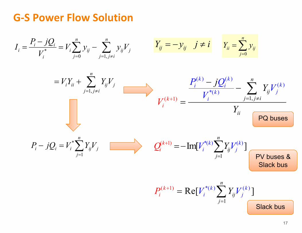
17

G‐S Power Flow Solution

*0 1,

n ni i

i i ij ij jj j j ii

P jQI V y y VV

ij ijY y j i

0

n

ii ijj

Y y

*

1

n

i i i ij jj

P jQ V Y V

( ) ( )( )

*(( 1) 1

),

n

ijj j

k kki i

kk i

i

i

ii

jj YP Q V

YV

V

*( ) ( )1)

1

( Im[ ] n

ijj

kk ki ji V Y VQ

*

1

(( )1) ) (Re[ ] k ki j

nk

i ijj

YP V V

1,

n

i ii ij jj j i

VY Y V

PQ buses

PV buses &Slack bus

Slack bus

18

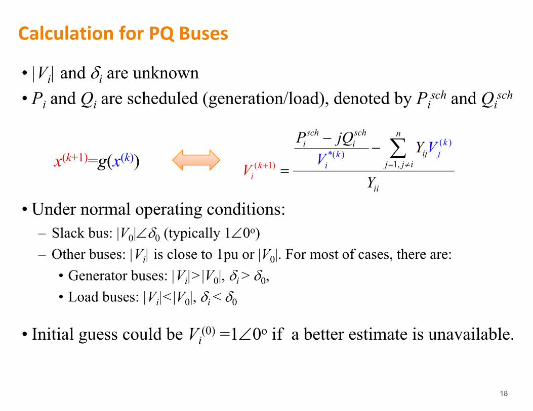
• |Vi| and i are unknown• Pi and Qi are scheduled (generation/load), denoted by Pi

sch and Qisch

• Under normal operating conditions:– Slack bus: |V0|0 (typically 10o)– Other buses: |Vi| is close to 1pu or |V0|. For most of cases, there are:

• Generator buses: |Vi|>|V0|, i > 0, • Load buses: |Vi|<|V0|, i < 0

• Initial guess could be Vi(0) =10o if a better estimate is unavailable.

( )*( )

1) 1,(

kjk

sch sch ni i

ijj jk i

iii

i

P jQ Y

Y

VV

V

x(k+1)=g(x(k))

Calculation for PQ Buses

19

Calculation for PV Buses

• Pi=Pisch and |Vi| are specified

• Starting from an initial estimate of i(0) Vi

(0)=|Vi| i(0)

• Since |Vi| is specified, only VI,i(k+1)=Im[Vci

(k+1)] is retained

• Continue the iterations until

or, the power mismatch, i.e. the largest element in P and Q <

• Using acceleration factor =1.3 to 1.7

*( ) ( )1)

1

( Im[ ] n

ijj

kk ki ji V Y VQ

( )

*(

( 1

( 1))

)

1,

k

jk

ki

kc

sch

i

ni

ijj j i

ii

i

P j YV

VY

Q V

2( 1) ( 1), ,

2| | ( ) k kR i I iiV VV

( 1) ( 1),

( ) (,,

),| | | | k k k

R i Ik

i I iR iV VV V

Update Vi(k+1)=VR,i

(k+1)+j VI,i(k+1)

( )*( )

( )

( 1)

( 1, ( )1) ( )

k

jkk ki

sch ni

ijj j

ii

ii

k

kic i

iP j Y

YV

V VVVQ

20

• At bus i:

• At bus j:

• Power loss in line i – j:

0 0( )ij l i ij i j i iI I I y V V y V

0 0( )ji l j ij j i j jI I I y V V y V

ij i ijS V I

ji j jiS V I

Lij ij jiS S S

yij

Calculation of Line Flows and Losses

*( 1) ( 1( 1) ( 1

1

)) k ki j

k ki i

n

ijj

P Q V Vj Y

Calculation for Slack Bus

21

Example 6.7 (slack bus + 2 P‐Q buses) y23=10-j20

y13=10-j30 y23=16-j32

( )*( )

1) 1,(

kjk

sch sch ni i

ijj jk i

iii

i

P jQ Y

Y

VV

V

Using the G-S method to find the power flow solution: (a) Determine the voltage phasors at P-Q buses 2 and 3

accurate to 4 decimal places(b) Find the slack bus real and reactive power(c) Determine the line flows and losses. Show line flow

directions in a power-flow diagram(Solve P1, Q1, |V2|, 2, |V3|, 3, Sij and Slij)

P1, Q1

|V2|, 2|V3|, 3

Step 1. Check what are known

Step 2. Set initial estimates and start to iterate

=0.9825-j0.0310

… …

P-Q

P-Q

22

*

1

n

i i i ij jj

P jQ V Y V

Step 3. Calculate P and Q of the slack bus

Step 4. Calculate line currents, flows and losses

0( )ij ij i j i iI y V V y V

0( )ji ij j i j jI y V V y V

ij i ijS V I

ji j jiS V I

Lij ij jiS S S

23

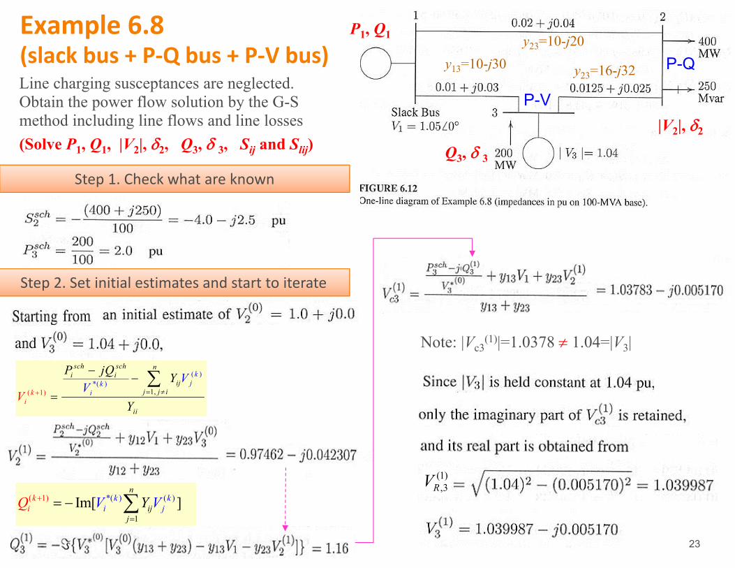
Example 6.8(slack bus + P‐Q bus + P‐V bus)Line charging susceptances are neglected. Obtain the power flow solution by the G-S method including line flows and line losses(Solve P1, Q1, |V2|, 2, Q3, 3, Sij and Slij)

y23=10-j20y13=10-j30 y23=16-j32

Note: |Vc3(1)|=1.0378 1.04=|V3|

P1, Q1

|V2|, 2

Q3, 3

Step 1. Check what are known

Step 2. Set initial estimates and start to iterate

(1),3RV

P-Q

P-V

( )*( )

1) 1,(

kjk

sch sch ni i

ijj jk i

iii

i

P jQ Y

Y

VV

V

*( ) ( )1)

1

( Im[ ] n

ijj

kk ki ji V Y VQ

24

( )*( )

1) 1,(

kjk

sch sch ni i

ijj jk i

iii

i

P jQ Y

Y

VV

V

*( ) ( )1)

1

( Im[ ] n

ijj

kk ki ji V Y VQ

2 ( 1)3

( 21)3 1.0 Im[4 ]Re[ { }] k

ck VV

(3)3(4)3(5)3(6)3(7)3

1.03954 0.00833

1.03978 0.00873

1.03989 0.00893

1.03993 0.00900

1.03995 0.00903

c

c

c

c

c

V j

V j

V j

V j

V j

( )*(

( 1

( 1))

)

1,

k

jkk

c

sch ni

ijj j

ii

i i

i

kiQ Y V

V

P

YV

j

Bus 2 (P‐Q): Solve |V2|, 2 Bus 3 (P‐V): Solve Q3, 3

Bus 1 (V‐): P1, Q1

*

1

n

i i i ij jj

P jQ V Y V

25

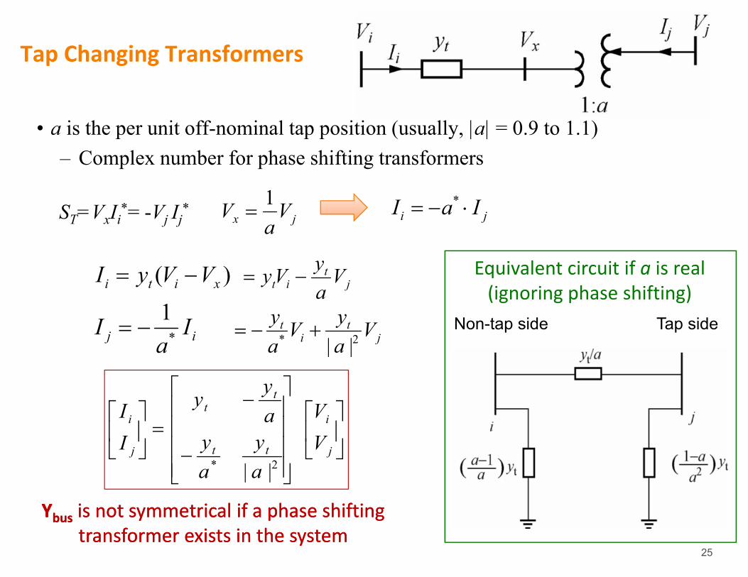
Tap Changing Transformers

• a is the per unit off-nominal tap position (usually, |a| = 0.9 to 1.1)– Complex number for phase shifting transformers

1x jV V

a

*i jI a I

( )i t i xI y V V tt i j

yy V Va

*1

j iI Ia

* 2| |t t

i jy yV Va a

* 2

| |

tt

i i

t tj j

yyI Vay yI Va a

ST=VxIi*= -Vj Ij

*

Non-tap side Tap side

Ybus is not symmetrical if a phase shifting transformer exists in the system

Ybus is not symmetrical if a phase shifting transformer exists in the system

Equivalent circuit if a is real (ignoring phase shifting) 

26

Newton‐Raphson Method

• Based on Taylor’s series expansion at an initial estimate of the solution

• Ignore all terms with orders 2

( )f x c(0) (0)( )f x cx

2(0) (0)(0) (0) 2(0)

2

1( ) ( ) ( )2

( )!

dfd

d ff xx x cdxx

(0 ) (0 )( (00 ) )() )( cdfdx

x f x c

＝

(0)0)

(0)

(

( )dfdx

cx

Comparison: G-S method ignores all differential terms (orders 1)

(1) (0 (0))x x x

27

• Iteration 1: (0)(1)

• Iteration k+1: (k) (k+1)

• Until

• f(x)=c is actually approximated by its tangent line at x=x(k).

(1) (0) ((0) (0)

0) (0)

(0) (0)

(0)

( ) ( )

( )df dfd

x x c c f x

x

x

x

x

d

x

＝ ＋ ＝

( )( ) ( )

( 1) ( ) ( ) (

( )

)

( )( ) ( )

( )k kk k k

k

kk

kdfx x x c c fdf

dx d

x x

x

x

＝ ＋ ＝

(( ) ( )) ( )( ( )) kk kf xd cf xx

xd

( )(

)

)

(( )

kk

kdfc

dx

x

( 1) ( ) | | k kx x

28

Example 6.42( ) 3 12 9df x x x

dx

(0) (0) 3 2( ) 0 [(6) 6(6) 9(6) 4] 50c c f x

Let x(0)=6

(0) 2( ) 3(6) 12(6) 9 45dfdx

(0)(0)

(0)

50 1.111145( )

cx dfdx

x(0)x(1)

(1) (0) (0) 6 1.1111 4.8889x x x

(2) (1) (1) 13.44314.8889 4.278922.037

x x x

(5) (4) (4) 0.00954.0011 4.00009.0126

x x x

(3) (2) (2) 2.99814.2789 4.040512.5797

x x x

(4) (3) (3) 0.37484.0405 4.00119.4914

x x x x(2)

(0)c

(0)x

( 1

( )

) )( )

( ( )

( )

k kk

kdfdx

xx cx f

＝

29

N‐dimensional System

(1( ( )(1) ( ) ( )) )1k k kk k kX X XX J C

( )1( )

( ) 2

( )

k

kk

kn

x

xX

x

( )1 1

( )( ) 2 2

( )

( )

( )

( )

k

kk

kn n

c f

c fC

c f

( )f x c

1 1 2 1

2 1 2 2

1 2

( , , , )( , , , )

( , , , )

n

n

n n n

f x x x cf x x x c

f x x x c

( ) ( ) ( )1 1 1

1 2

( ) ( ) ( )2 2 2( )

1 2

( ) ( ) ( )

1 2

( ) ( ) ( )

( ) ( ) ( )

( ) ( ) ( )

k k k

n

k k kk

n

k k kn n n

n

f f fx x xf f fx x xJ

f f fx x x

Jacobian Matrix:

1( 1) ( ) ( )) (( ) ( )( ) kkkk k kx x xx df c

dx

＋

( ) ( )( )k kc c f x

30

Example 6.5• Use the N-R method to find the intersections of the curves

2 21 2 4x x

12 1xe x 1

1 22 21x

x xJ

e

If x1(0)=2, x2

(0)= -2:k C J x x

1 -4.0000 4.0000 -4.0000 -0.6424 1.3576

-4.3891 7.3891 1.0000 0.3576 -1.6424

2 -0.5406 2.7152 -3.2848 -0.2989 1.0587

-1.2445 3.8869 1.0000 -0.0825 -1.7249

3 -0.0962 2.1173 -3.4499 -0.0530 1.0056

-0.1576 2.8825 1.0000 -0.0047 -1.7296

4 -0.0028 2.0112 -3.4592 -0.0014 1.0042

-0.0040 2.7336 1.0000 -0.0000 -1.7296

5 -0.0000 2.0083 -3.4593 -0.0000 1.0042

-0.0000 2.7296 1.0000 -0.0000 -1.7296

J (k) tells the fastest direction (gradient) seen from point k on the path toward a solution

31

Compared to the Gauss‐Seidel Method

• Since higher-order terms are ignored, the N-R method also needs the initial estimation to be sufficiently close to the actual solution

• The N-R method converges much faster– N-R method: quadratic convergence (ignoring the 2nd and

higher orders)– G-S method: linear convergence (ignoring the 1st and higher

orders)• The N-R method has more computational complexity:

– Requires [J(k)]-1 during each iteration, which is computationally intense

32

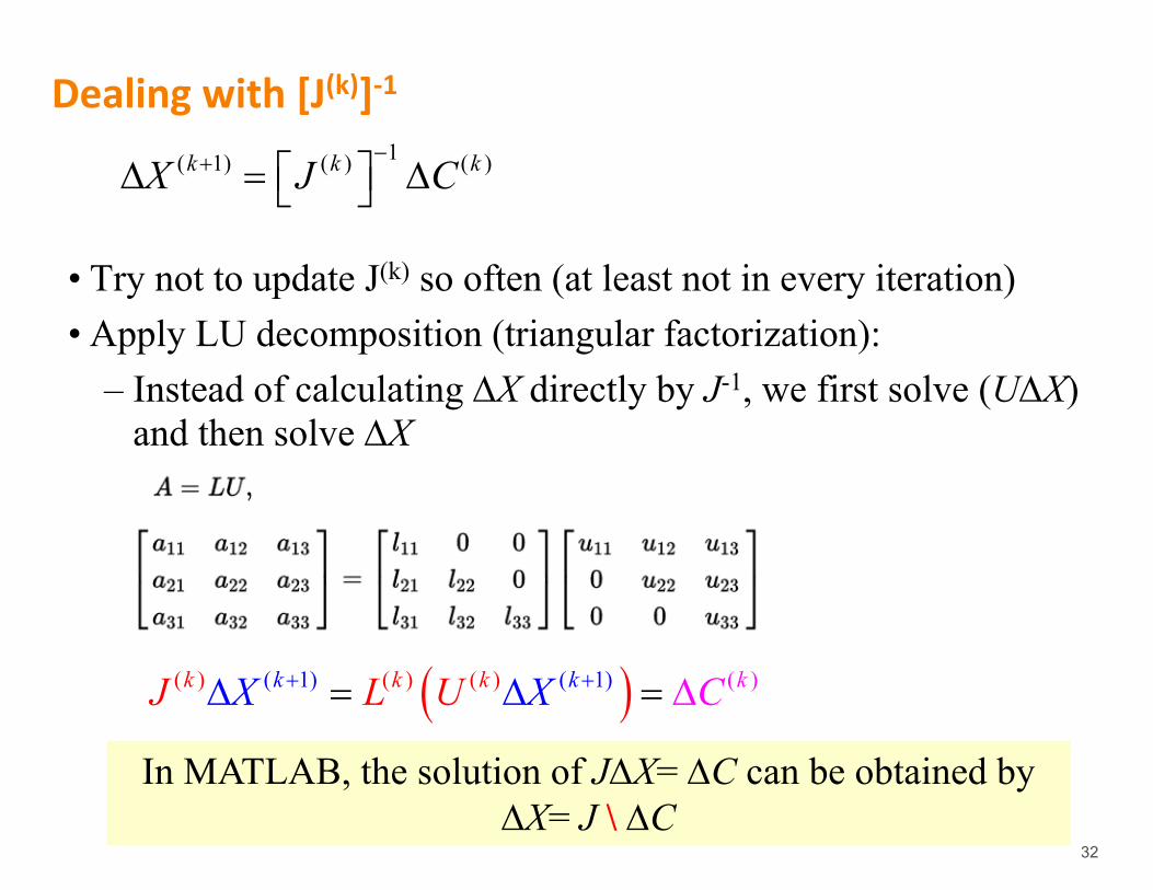
Dealing with [J(k)]‐1

• Try not to update J(k) so often (at least not in every iteration)• Apply LU decomposition (triangular factorization):

– Instead of calculating X directly by J-1, we first solve (UX) and then solve X

1( 1) ( ) ( )k k kX J C

( 1) ( 1)( ) ( )( ) ( )k kk kk kJ L U X CX

In MATLAB, the solution of JX= C can be obtained byX= J \ C