Future hydrological extremes: the uncertainty from ... · 3Irstea, UR HHLY Hydrology-Hydraulics,...

Earth Syst. Dynam., 6, 267–285, 2015

www.earth-syst-dynam.net/6/267/2015/

doi:10.5194/esd-6-267-2015

© Author(s) 2015. CC Attribution 3.0 License.

Future hydrological extremes: the uncertainty from

multiple global climate and global hydrological models

I. Giuntoli1,2,3, J.-P. Vidal3, C. Prudhomme2, and D. M. Hannah1

1School of Geography, Earth & Environmental Sciences, University of Birmingham, Birmingham B15 2TT, UK2Centre for Ecology and Hydrology, Wallingford OX10 8BB, UK

3Irstea, UR HHLY Hydrology-Hydraulics, Lyon, France

Correspondence to: I. Giuntoli ([email protected])

Received: 4 December 2014 – Published in Earth Syst. Dynam. Discuss.: 6 January 2015

Revised: 11 April 2015 – Accepted: 25 April 2015 – Published: 18 May 2015

Abstract. Projections of changes in the hydrological cycle from global hydrological models (GHMs) driven

by global climate models (GCMs) are critical for understanding future occurrence of hydrological extremes.

However, uncertainties remain large and need to be better assessed. In particular, recent studies have pointed

to a considerable contribution of GHMs that can equal or outweigh the contribution of GCMs to uncertainty in

hydrological projections. Using six GHMs and five GCMs from the ISI-MIP multi-model ensemble, this study

aims: (i) to assess future changes in the frequency of both high and low flows at the global scale using control

and future (RCP8.5) simulations by the 2080s, and (ii) to quantify, for both ends of the runoff spectrum, GCMs

and GHMs contributions to uncertainty using a two-way ANOVA. Increases are found in high flows for northern

latitudes and in low flows for several hotspots. Globally, the largest source of uncertainty is associated with

GCMs, but GHMs are the greatest source in snow-dominated regions. More specifically, results vary depending

on the runoff metric, the temporal (annual and seasonal) and regional scale of analysis. For instance, uncertainty

contribution from GHMs is higher for low flows than it is for high flows, partly owing to the different processes

driving the onset of the two phenomena (e.g. the more direct effect of the GCMs’ precipitation variability on

high flows). This study provides a comprehensive synthesis of where future hydrological extremes are projected

to increase and where the ensemble spread is owed to either GCMs or GHMs. Finally, our results underline the

need for improvements in modelling snowmelt and runoff processes to project future hydrological extremes and

the importance of using multiple GCMs and GHMs to encompass the uncertainty range provided by these two

sources.

1 Introduction

The ongoing intensification of the water cycle at the global

scale is expected to continue in the coming decades (Hunt-

ington, 2006; Stott et al., 2010). Projected changes in cli-

mate variables from global climate models (GCMs) indi-

cate an increase in the frequency of hydrological extremes

(Tebaldi et al., 2006; Seneviratne et al., 2012; Sillmann et al.,

2013; Kharin et al., 2013). These hydrological shifts go hand

in hand with a growing world population that will become

ever more vulnerable with respect to access to water and

food, and resilience to natural hazards (Lavell et al., 2012).

In this context, global multi-model ensembles yield a valu-

able opportunity for climate projections and impact assess-

ments. In hydrology, multi-model ensemble experiments –

consisting of global hydrological models (GHMs) fed by in-

put forcing simulated by GCMs – can be used to project fu-

ture changes in the water cycle and future hydrological ex-

tremes, using modelled variables such as precipitation, runoff

and soil moisture. In recent years, a number of studies have

assessed the future changes in the global water cycle (e.g.

Nohara et al., 2006; Hirabayashi et al., 2008; Sheffield and

Wood, 2008). Although many of these studies have a rep-

resentative number of GCMs in their ensembles, they rarely

comprise more than one GHM, and this presents a limitation

considering that GHMs provide more uncertainty than pre-

Published by Copernicus Publications on behalf of the European Geosciences Union.

268 I. Giuntoli et al.: Future global hydrological extremes uncertainty

viously thought (Haddeland et al., 2011; Hagemann et al.,

2013; Schewe et al., 2013; Prudhomme et al., 2014). In addi-

tion, the coarse temporal and spatial resolution of the climate

signal used in these studies does not reflect well the potential

changes in sub-monthly extreme events at the regional and

local scale (Forzieri et al., 2014).

Recently, model inter-comparison projects like WaterMIP

(Haddeland et al., 2011) and ISI-MIP (Warszawski et al.,

2014) have made it possible to include multiple GCMs and

GHMs in global impact studies at unprecedented temporal

(up to daily) and spatial (0.5◦) resolution, thereby providing

frameworks for consistent assessments of the terrestrial wa-

ter cycle.

The ISI-MIP data set has been used to assess future

changes in runoff at global and regional scales. Dankers et al.

(2013) explored changes in a 30-year return period of river

flow showing that flood hazard is projected overall to in-

crease globally, although not uniformly, and that decreases

occur mainly in areas where the hydrograph is dominated by

spring snowmelt. Schewe et al. (2013) assessed future water

scarcity by analysing changes in mean annual runoff together

with global population patterns, showing how the number of

people living in water scarcity is projected to increase glob-

ally. Davie et al. (2013) investigated runoff changes across

models by grouping GHMs into hydrological and biome (in-

cluding CO2 and vegetation dynamics) models, showing that

while both types agree on the sign of runoff change for

most regions of the world (with contrasting exceptions like

West Africa where biome models moisten and hydrologi-

cal models dry), models accounting for varying CO2 yield

more runoff than those with constant CO2. Prudhomme et al.

(2014) examined the future frequency of droughts using a

variable threshold method on daily runoff. They identified

drought hotspots globally and observed, similarly to Davie

et al. (2013), how biome models accounting for varying CO2

concentrations tend to project more runoff with increasing

CO2 than the hydrological models. All of these studies em-

phasize how both GCM and GHM uncertainty contribute to

the spread in projected changes in the hydrological cycle.

Their findings highlight the importance of including differ-

ent types of GHMs and GCMs for making comprehensive

assessments of uncertainty in climate impact studies.

In this context, modelling-induced uncertainty (i.e. inter-

model spread of GCMs and GHMs) has been expressed by

looking at the variance across both types of models. For

example, Schewe et al. (2013) and Dankers et al. (2013)

used the ratio of the variances of GCM and GHM results

(for GCMs: variance of the change across all GCMs for

each GHM, then averaged over all of the GHMs; and vice

versa for GHMs). Similarly, using WaterMIP data, Hage-

mann et al. (2013) expressed the spread due to the choice of

model type using the standard deviation of GCMs and GHMs

(for GCMs: the mean across all GHMs for each GCM, and

standard deviation of the GCMs; and vice versa for GHMs).

Prudhomme et al. (2014) omit the partition into GCM/GHM

and express the uncertainty through the signal-to-noise ra-

tio (by grouping results per type of model) in order to infer

which global model type in the ensemble brings about high-

est agreement.

The studies cited above have provided useful knowledge

on climate change impacts on the water cycle using the ISI-

MIP data set, however, a synthesis of future projections for

high and low flows along with a consistent estimation of un-

certainties is still missing. The present study builds on the

work on low flows of Prudhomme et al. (2014), but intro-

duces several new aspects. Firstly, low flows (Q10) are now

analysed using an improved index extraction. The variable

threshold method used in Prudhomme et al. (2014) has been

revisited to overcome a limitation of the 30-day moving win-

dow for which grid cells were assigned lower threshold val-

ues than the theoretical threshold assigned (Q10) (i.e. a ten-

dency to capture fewer occurrences, an effect perhaps at-

tributable to GHMs’ slow emptying of reservoirs during the

recession phase). A shorter 5-day fixed time window elim-

inates this effect. Note that, in order to gather further data

for the estimate of the quantile flow, the period of analysis

was increased from 30 to 34 years, starting 4 years earlier

(1972 for control and 2066 for future). Secondly, we now

analyse high flows (Q95), with the same method used for

low flows (5-day fixed-window variable-threshold method).

Dankers et al. (2013), who also analysed high flows, have

focused on a different metric (annual extreme monthly flood

peak with 30-year return level), as their aim was to describe

changes in flood hazard, while our focus is on change in fre-

quency of high flow days. In our study high and low flows

are hence identified jointly with the same ensemble of five

GCMs and six GHMs. While comprising the same number

of GCMs, the ensemble used by Prudhomme et al. (2014)

uses one additional GHM (JULES) and Dankers et al. (2013)

uses three additional GHMs (JULES, LPJmL, MATSIRO).

We did not use these additional GHMs as they showed large

areas with long pools of zero values hindering the index ex-

traction, making them unsuitable for our analysis, especially

for the low flows; additionally, JULES was run at a coarser

resolution (1.25–1.875◦ vs. 0.5–0.5◦) that would potentially

influence the uncertainty analysis. Thirdly, we assess system-

atically the relative contribution of GHMs and GCMs to un-

certainty using an analysis of variance (ANOVA) framework

as in e.g. Yip et al. (2011) and Sansom et al. (2013). This un-

certainty assessment moves beyond the signal-to-noise ratio

by Prudhomme et al. (2014), as the quantification of each

source (GCM/GHM) to total uncertainty allows us to de-

scribe the spatial variability of the contributions grid cell

per grid cell. While Dankers et al. (2013) and Schewe et al.

(2013) partition GCM/GIM uncertainty using ratios between

the variances, our ANOVA approach adds the contribution of

the error (or residual) to the partition of the variance along

with post hoc testing on the residuals for model adequacy.

We thus describe how high and low flows and inherent un-

certainty vary at the seasonal and spatial scale, identifying

Earth Syst. Dynam., 6, 267–285, 2015 www.earth-syst-dynam.net/6/267/2015/

I. Giuntoli et al.: Future global hydrological extremes uncertainty 269

areas where we have more confidence in the climate or in the

hydrology (i.e. uncertainty is owed to GCMs or GHMs). Fi-

nally, to understand how the variance of the changes differs

regionally, we carry out analysis at the regional scale express-

ing the ANOVA sum-of-squares of each source using homo-

geneous geo-climate regions (Köppen–Geiger). This allows

for an improved understanding of how the climate and hy-

drological processes drive uncertainty for both runoff ends.

By comparing an ensemble of GCMs (5) and GHMs (6)

for future projections (2066–2099) against the historical pe-

riod (1972–2005), this study aims (i) to assess future high

and low flows changes at global and annual and seasonal

scales, and (ii) to quantify the uncertainty attributable to

GHMs and GCMs using ANOVA. In the next section, the

data set and the different steps of the methodology are de-

tailed. The results of projected hydrological extremes and

respective uncertainty are presented in Sect. 3 before dis-

cussing the important and wider implications of this research

in the fourth and final section.

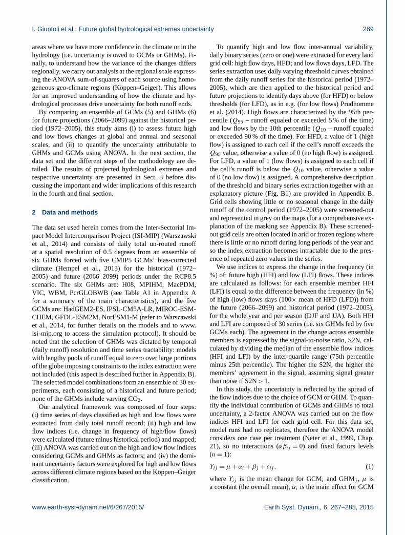
2 Data and methods

The data set used herein comes from the Inter-Sectorial Im-

pact Model Intercomparison Project (ISI-MIP) (Warszawski

et al., 2014) and consists of daily total un-routed runoff

at a spatial resolution of 0.5 degrees from an ensemble of

six GHMs forced with five CMIP5 GCMs’ bias-corrected

climate (Hempel et al., 2013) for the historical (1972–

2005) and future (2066–2099) periods under the RCP8.5

scenario. The six GHMs are: H08, MPIHM, MacPDM,

VIC, WBM, PcrGLOBWB (see Table A1 in Appendix A

for a summary of the main characteristics), and the five

GCMs are: HadGEM2-ES, IPSL-CM5A-LR, MIROC-ESM-

CHEM, GFDL-ESM2M, NorESM1-M (refer to Warszawski

et al., 2014, for further details on the models and to www.

isi-mip.org to access the simulation protocol). It should be

noted that the selection of GHMs was dictated by temporal

(daily runoff) resolution and time series tractability: models

with lengthy pools of runoff equal to zero over large portions

of the globe imposing constraints to the index extraction were

not included (this aspect is described further in Appendix B).

The selected model combinations form an ensemble of 30 ex-

periments, each consisting of a historical and future period;

none of the GHMs include varying CO2.

Our analytical framework was composed of four steps:

(i) time series of days classified as high and low flows were

extracted from daily total runoff record; (ii) high and low

flow indices (i.e. change in frequency of high/flow flows)

were calculated (future minus historical period) and mapped;

(iii) ANOVA was carried out on the high and low flow indices

considering GCMs and GHMs as factors; and (iv) the domi-

nant uncertainty factors were explored for high and low flows

across different climate regions based on the Köppen–Geiger

classification.

To quantify high and low flow inter-annual variability,

daily binary series (zero or one) were extracted for every land

grid cell: high flow days, HFD; and low flows days, LFD. The

series extraction uses daily varying threshold curves obtained

from the daily runoff series for the historical period (1972–

2005), which are then applied to the historical period and

future projections to identify days above (for HFD) or below

thresholds (for LFD), as in e.g. (for low flows) Prudhomme

et al. (2014). High flows are characterized by the 95th per-

centile (Q95 – runoff equaled or exceeded 5 % of the time)

and low flows by the 10th percentile (Q10 – runoff equaled

or exceeded 90 % of the time). For HFD, a value of 1 (high

flow) is assigned to each cell if the cell’s runoff exceeds the

Q95 value, otherwise a value of 0 (no high flow) is assigned.

For LFD, a value of 1 (low flows) is assigned to each cell if

the cell’s runoff is below the Q10 value, otherwise a value

of 0 (no low flow) is assigned. A comprehensive description

of the threshold and binary series extraction together with an

explanatory picture (Fig. B1) are provided in Appendix B.

Grid cells showing little or no seasonal change in the daily

runoff of the control period (1972–2005) were screened-out

and represented in grey on the maps (for a comprehensive ex-

planation of the masking see Appendix B). These screened-

out grid cells are often located in arid or frozen regions where

there is little or no runoff during long periods of the year and

so the index extraction becomes intractable due to the pres-

ence of repeated zero values in the series.

We use indices to express the change in the frequency (in

%) of: future high (HFI) and low (LFI) flows. These indices

are calculated as follows: for each ensemble member HFI

(LFI) is equal to the difference between the frequency (in %)

of high (low) flows days (100× mean of HFD (LFD)) from

the future (2066–2099) and historical period (1972–2005),

for the whole year and per season (DJF and JJA). Both HFI

and LFI are composed of 30 series (i.e. six GHMs fed by five

GCMs each). The agreement in the change across ensemble

members is expressed by the signal-to-noise ratio, S2N, cal-

culated by dividing the median of the ensemble flow indices

(HFI and LFI) by the inter-quartile range (75th percentile

minus 25th percentile). The higher the S2N, the higher the

members’ agreement in the signal, assuming signal greater

than noise if S2N> 1.

In this study, the uncertainty is reflected by the spread of

the flow indices due to the choice of GCM or GHM. To quan-

tify the individual contribution of GCMs and GHMs to total

uncertainty, a 2-factor ANOVA was carried out on the flow

indices HFI and LFI for each grid cell. For this data set,

model runs had no replicates, therefore the ANOVA model

considers one case per treatment (Neter et al., 1999, Chap.

21), so no interactions (αβij = 0) and fixed factors levels

(n= 1):

Yij = µ+αi +βj + εij , (1)

where Yij is the mean change for GCMi and GHMj , µ is

a constant (the overall mean), αi is the main effect for GCM

www.earth-syst-dynam.net/6/267/2015/ Earth Syst. Dynam., 6, 267–285, 2015

www.isi-mip.org

www.isi-mip.org


Figure 1. Change in the frequency (in %) of days under high (left) and low (right) flow conditions for the period 2066–2099 relative to

1972–2005, based on a multi-model ensemble (MME) experiment under RCP8.5 from five GCMs and six GHMs: (a) MME mean change

and associated (b) signal-to-noise ratio; (c) Proportion of variance per factor for the MME mean change: GCM (yellow), GHM (green),

Residual (red).

at the ith level, βj is the main effect for GHM at the j th level,

εij is the residual ≈N (0,σ 2)iid. Thus, the variance is parti-

tioned into two factors, GCMs and GHMs, plus the residu-

als. The results, expressed in terms of sum of squares, are

used to quantify the factors’ contributions to the total vari-

ance, here considered as uncertainty as in e.g. Sansom et al.

(2013). ANOVA models are reasonably robust against certain

types of departures from the model (e.g. error terms not being

exactly normally distributed). Nonetheless, the suitability of

the ANOVA model with the data at hand should be checked

for serious departures from the conditions assumed by the

model by looking at the residuals (Neter et al., 1999, Chap.

18) and testing their normality (e.g. Lilliefors test) and con-

stancy of variance (e.g. Hartley test). Unsatisfactory results

would require remedial measures like data transformation or

a modification of the model. To understand how variance dif-

fers between climate regions, the ANOVA sum of squares for

all model combinations are shown per Köppen–Geiger class.

We used the Köppen–Geiger data classification based on the

present day as proposed by Kottek et al. (2006) (a link to the

map is provided at the end of Table 1). A total of 15 (out

of 31) regions are considered leaving out under-represented

regions with too few grid cells (< 1000).

3 Results

Annual mean changes and associated S2N across all GHMs

and GCMs are shown for HFI and LFI in Fig. 1a and b.

For high and low flow indices, the mean changes vary spa-

tially and in magnitude (Fig. 2) but they are positive gener-

ally. This means increases in number of days with (i) high

flows, mostly over high northern latitudes; and (ii) low

flows, spread over all latitudes with hotspots in southern

Europe, southwestern and mid Latin America, southeastern

USA and southeastern Canada, lower parts of Central Africa,

north/northeastern China, and southwestern Australia. Re-

gions screened-out represent 14 and 18 % of land for HFI

and LFI, respectively. The S2N shows model agreement gen-

erally over the same regions for both indices (e.g. southern

Europe, south western and mid Latin America, southeastern

US). However, model agreement is found for HFI – but not



Figure 2. PDFs of mean changes in high (HFI) and low (LFI) flows, annually and per season (DJF and JJA) for North, Tropics, and South

latitude bands.

for LFI – over Alaska, eastern Canada, and northwestern and

eastern Russia. In some regions increases are not associated

with a strong S2N (e.g. for high flows over western China and

the Horn of Africa). Mean changes and S2N for boreal winter

(DJF) and summer (JJA), in Figs. 3 and 4 respectively, show

an increased intensity with very similar spatial patterns to

their annual counterparts in DJF for the high flows and in JJA

for low flows. Conversely, high flows in JJA show virtually

no change, while low flows in DJF show decreases at high

northern latitudes with high model agreement and increases

elsewhere with smaller model agreement (S2N). This can be

seen also in Fig. 2: the PDF (i.e. the density of the mean

change percentage) stretches towards higher mean changes

for high flows in DJF and for low flows in JJA. Global re-

sults are dominated by boreal seasonality (high flow changes

dominant in DJF, and low flow changes dominant in JJA) as

the majority of global land cells 65 % (of unmasked land)

are located north of latitude 23.5◦. The remainder of the land

cells (35 %) are located within the Tropics and south latitude

bands, and depict weak changes for high flows in all seasons,

and increased changes for low flows in all seasons, though

JJA’s are more marked.

The results of the ANOVA across the 30 members of

HFI and LFI are shown in Fig. 1c; they are expressed, for

each factor, as the proportion of sum of squares divided by

the total sum of squares (refer to Appendix C for residuals

testing for model adequacy). For the high flows, the vari-

ance is explained mostly by the GCMs (yellow, 47 % of un-

masked land, Fig. 1c), although the GHMs are the major fac-

tor over western Europe and central Canada (green, 28 %

of unmasked land, Fig. 1c). For low flows, the proportions

change: the GCMs (43 %) remain the major contributors over

the globe, but GHMs (35 %) increase to a relative influence

closer to the GCMs, and become the major factor in some

northern (e.g. northeastern Russia) and southern (e.g. south-

ern Africa, southwestern Australia) regions. Seasonal results

(Figs. 3c and 4c) are very similar to their annual counter-

parts in the case of high flows in DJF and low flows in JJA,

whereas for high flows in JJA and for low flows in DJF higher

residual rates (i.e. decreased overall GHM and GCM contri-

butions) are found, perhaps owing to fewer events occurring

in these seasons for both low and high flow indices.

To capture better the spatial distribution of the major

sources of uncertainty, ANOVA results are aggregated by

climatic homogeneous regions based on the climatological

Köppen–Geiger classification. Scatterplots in Fig. 5 show

the proportions of sums of squares of GHMs (y-axis) vs.

GCMs (x-axis); medians for each climatic region are shown

as their class letter and summarize the prominent factor of

uncertainty. For both high and low flows calculated over the

year and seasonally, uncertainty in equatorial regions (A) is

dominated by GCMs (median closest to the x-axis); while

in snow-dominated climate (D) it is dominated by GHMs

(median closest to the y-axis). In warm temperate regions



Table 1. Summary of mean changes, signal-to-noise S2N, and sources of variance for high and low flows at the annual and seasonal (DJF,

JJA) scale, and at the global and climate region scale. The first source of variance is shown in bold, the second one in italic font.

YEAR DJF JJA

Köppen– Area Mean1 Signal2 Source of variance Mean Signal to Source of variance Mean Signal to Source of variance

Geiger change to noise GCM GHM Resid. change noise GCM GHM Resid. change noise GCM GHM Resid.

Class∗ [km2] [%] adim. [%] [%] [%] [%] adim. [%] [%] [%] [%] adim. [%] [%] [%]

HIGH FLOWS

Equatorial

1 Af 2468 3.1 0.5 65.5 14.2 20.3 3.4 0.5 64.4 11.4 24.3 3.2 0.6 64.0 12.4 23.6

2 Am 1836 1.4 0.5 61.6 15.5 22.9 2.8 0.4 60.2 14.8 25.0 0.7 0.9 65.9 11.0 23.1

3 Aw 6017 1.6 0.6 52.7 20.4 27.0 2.9 0.4 56.3 18.3 25.5 0.5 0.9 47.0 19.7 33.3

Arid

4 Bwk 3095 4.1 0.5 49.7 19.8 30.5 5.5 0.4 47.1 20.7 32.3 2.3 0.7 42.9 20.3 36.8

5 Bwh 3139 1.2 0.6 39.3 28.5 32.2 3.1 0.6 35.6 29.6 34.8 0.1 0.7 37.7 25.3 37.1

6 BSk 4255 6.4 0.4 40.5 25.1 34.4 7.0 0.4 39.6 23.9 36.4 5.1 0.5 36.2 25.5 38.3

Warm temp.

7 Cfa 2955 −0.6 0.6 56.1 26.8 17.1 −0.5 0.4 57.1 22.9 20.0 −0.8 0.8 55.4 20.1 24.5

8 Cfb 2360 0.4 0.9 45.0 35.9 19.0 1.8 0.6 40.5 37.7 21.9 −0.5 1.0 45.4 29.1 25.5

9 Csa 1099 −1.2 1.5 45.3 32.8 21.9 −0.8 1.3 50.8 30.2 19.0 −2.0 1.9 31.0 30.5 38.5

10 Cwa 1504 0.9 0.6 43.8 28.0 28.2 0.9 0.4 45.6 27.6 26.8 1.1 0.8 49.8 23.9 26.3

Snow

11 Dfb 4459 5.4 0.7 42.7 37.1 20.2 17.5 0.7 38.2 40.3 21.5 −1.1 0.8 57.3 21.6 21.1

12 Dfc 11008 18.6 1.2 38.0 38.8 23.2 37.5 1.0 36.0 39.7 24.2 0.2 0.7 39.7 34.2 26.2

13 Dfd 1405 27.4 1.1 42.7 22.4 34.9 39.8 0.9 38.1 26.2 35.6 7.4 0.4 13.6 55.6 30.8

14 Dwb 1311 6.7 0.5 29.1 46.1 24.8 11.0 0.4 25.7 41.9 32.3 1.4 0.3 35.0 41.9 23.1

Polar

15 ET 5937 26.3 1.3 42.9 36.1 20.9 40.6 1.2 43.7 32.2 24.1 5.5 0.5 34.3 41.0 24.7

Global 128.9M 6.5 0.7 46.5 28.0 25.5 11.8 0.6 45.5 27.5 27 1.3 0.8 45.0 25.4 29.7

LOW FLOWS

Equatorial

1 Af 2463 14.6 0.5 58.7 18.1 23.1 12.7 0.3 56.5 20.4 23.1 15.4 0.5 50.1 17.1 32.8

2 Am 1834 23.7 0.7 57.0 25.2 17.8 19.7 0.4 50.5 29.1 20.4 27.1 0.7 59.5 18.1 22.4

3 Aw 5997 21.7 0.7 52.4 28.5 19.0 18.4 0.5 48.2 29.8 22.0 25.7 0.6 50.8 28.3 20.9

Arid

4 Bwk 2927 15.6 0.5 41.4 31.0 27.6 14.3 0.5 40.0 31.1 28.9 17.1 0.4 38.4 32.1 29.5

5 Bwh 2821 20.2 0.6 32.1 42.6 25.3 18.4 0.5 29.2 42.8 28.0 22.2 0.6 30.3 42.9 26.7

6 BSk 2693 14.3 0.6 35.9 32.1 32.0 13.5 0.6 35.0 31.2 33.7 15.1 0.5 33.8 33.3 33.0

Warm temp.

7 Cfa 2950 18.2 1.0 49.1 32.9 18.1 17.6 0.7 47.5 32.4 20.0 19.1 0.9 44.1 30.9 25.0

8 Cfb 2358 20.2 1.1 51.7 32.3 16.0 15.2 0.8 43.7 36.4 19.9 24.4 1.0 46.2 33.6 20.1

9 Csa 1096 35.7 1.4 47.0 37.6 15.5 31.0 1.3 48.7 35.8 15.5 41.9 1.4 41.0 37.7 21.3

10 Cwa 1500 18.5 0.8 42.0 39.4 18.5 18.1 0.7 39.5 39.8 20.7 18.4 0.7 44.7 34.1 21.2

Snow

11 Dfb 4440 15.8 0.8 50.6 28.1 21.3 4.1 0.5 29.8 43.5 26.7 26.3 0.9 52.4 26.0 21.6

12 Dfc 10920 8.7 0.5 33.6 44.8 21.7 −2.0 1.5 17.4 45.1 37.5 25.0 0.8 38.9 43.1 18.1

13 Dfd 1402 −2.5 0.7 15.3 59.3 25.4 −5.7 2.3 16.8 40.1 43.1 4.4 0.2 14.5 66.4 19.1

14 Dwb 1306 9.5 0.3 26.8 48.5 24.7 9.9 0.3 23.3 47.3 29.4 11.4 0.5 31.7 46.7 21.5

Polar

15 ET 5650 3.4 0.5 29.8 45.0 25.2 −1.7 2.1 20.2 37.9 41.9 14.3 0.5 35.2 46.4 18.3

Global 122M 16.1 0.7 43.1 34.8 22.1 11.8 0.8 36.6 35.9 27.6 21.5 0.7 42.5 34.2 23.3

1st, 2nd Source of variance.1 Mean change weighted over grid cells’ surface areas. 2 Signal-to-noise weighted over grid cells’ surface areas.∗ The map can be downloaded at: http://koeppen-geiger.vu-wien.ac.at/pdf/kottek_et_al_2006_A4.pdf.

(C), uncertainty is slightly higher for GCMs than GHMs. In

arid regions (B), the variance is not well explained by ei-

ther GCMs or GHMs (median farthest from 1; i.e. residu-

als explain most of the variance), suggesting that reproduc-

ing hydroclimatology over these regions represents a chal-

lenge for both GCMs and GHMs. The ANOVA results for the

whole year and those for winter and summer seasons (DJF

and JJA shown in Figs. 3c and 4c) are quantified further in

Table 1. This table provides a breakdown with both the re-

gional and global results expressed for mean changes, S2N

and percentage of sum of squares per factor at the annual and

seasonal (DJF and JJA) scale. Looking jointly at the annual

and seasonal results in Table 1, it is clear that the widespread

dominance of the GCMs’ contribution to uncertainty is out-

weighed by the GHMs in the snow- and ice-dominated re-

gions (D). This pattern is visible also on the scatterplots

(Figs. 5 and 6) with the GHM uncertainty-dominated regions

(near the y-axis) often populated by D regions for both HFI

and LFI (although to a lesser extent for the former).


http://koeppen-geiger.vu-wien.ac.at/pdf/kottek_et_al_2006_A4.pdf


Figure 3. As Fig. 1, for the season DJF.

4 Discussion and conclusions

Using six global hydrological models (GHMs) fed by five

global climate models (GCMs) under the RCP8.5 scenario,

this study aimed to assess future high and low flow changes

globally by the 2080s, and to quantify the uncertainty at-

tributable to GHMs and GCMs. We decided to focus solely

on the uncertainty coming from GHMs and GCMs using as

many ensemble members (from the ISI-MIP project data set)

as possible under the RCP8.5, in which change signals are

expected to be larger (i.e. emissions continue to rise leading

to global radiative forcing levels of 8.5 Wm−2 by the end of

the 21st century). The hydrological simulations used in this

study do not account for anthropogenic influences (e.g. water

abstraction, augmentation and artificial storage) or land-use

changes.

High and low flow changes in the future (2066–2099) rel-

ative to the control period (1972–2005) exhibit a number of

robust large-scale features. Increases in high flow days were

found at northern latitudes, with a strong signal over east-

ern Canada, Scandinavia, northwestern Russia, and around

the Bering Sea (eastern Russia and Alaska). Increases in low

flow days were found in southern Europe, southwestern and

central Latin America, southeastern USA, more southerly

parts of Central Africa, and southwestern Australia. These

patterns are largely consistent with the few other studies car-

ried out on runoff at the global scale with several GHM–

GCM combinations: e.g. for high flows (Hirabayashi et al.,

2013), low flows (Van Huijgevoort et al., 2013; Prudhomme

et al., 2014) and for mean flows (Davie et al., 2013; Schewe

et al., 2013; Hagemann et al., 2013). More specifically, the

comparison of flood hazard patterns by Dankers et al. (2013)

with the changes in the occurrence of high flow days from our

study reveals some similarities, mostly northern North Amer-

ica and Northern Asia, while in some regions like northeast-

ern Europe patterns are opposite. Low flow patterns are sim-

ilar to Prudhomme et al. (2014) although they find a weaker

S2N.

In this study we provide for the first time a comprehen-

sive assessment of both ends of the runoff spectrum at the

same time using the same data set globally. Moreover, we

undertake a consistent partition of uncertainty via ANOVA

for both high and low flows, showing that GCMs provide

the largest uncertainty, although the GHM contribution can

be substantial in particular regions. The results from our

ANOVA framework are consistent with other global studies



Figure 4. As Figs. 1 and 3, for the season JJA.

based on the ratios between the variances (or standard de-

viations) of ensemble members averaged per type of model

(Dankers et al., 2013; Schewe et al., 2013; Hagemann et al.,

2013). In particular, uncertainty results that Dankers et al.

(2013) expressed with GCM/GHM variance are in agree-

ment with our findings for high flows in the Southern Hemi-

sphere, mainly driven by GCM uncertainty, whereas there is

less agreement for the Northern Hemisphere (in North Amer-

ica, Central Canada is GCM-driven uncertainty, whereas it is

GHM driven in our results). Uncertainty results for low flows

from Prudhomme et al. (2014), expressed as S2N ratio, are

not directly comparable, but as will be discussed later, the in-

clusion of the JULES GHM in their ensemble has pointed to

lower model agreement (i.e. increased uncertainty).

At the regional level, the uncertainty partition enables us

to delineate in which climate region each factor (GCMs or

GHMs) provides the largest uncertainty at the annual and

seasonal scales. Notably, for snow- and ice-dominated po-

lar regions, and for arid zones, GHMs bring about the largest

portion of uncertainty, especially for low flows. This is likely

to reflect uncertainty in the way the hydrological storage–

release processes can modify the climate signal, particularly

where these storage components are relatively large or water

residence times high – hence the importance of considering

several GHMs in studying changes in high and low flows.

GCM and GHM uncertainty shares are similar for HFI and

LFI globally, although the spatial patterns differ slightly (e.g.

northeastern Russia, southwestern Australia and Alaska are

GCM driven in HFI, and GHM driven in LFI). This could re-

flect different dominant processes for high and low flow gen-

eration, with high flow events mainly driven by precipitation

inputs or snow/ice-melt (i.e. atmospheric-driven processes);

whereas low flows event develop over longer durations and

are influenced more by land-surface processes like evapo-

ration, infiltration and storage, which are simulated by the

GHMs, each one with its own scheme and parametrization:

e.g. for evapotranspiration, Penman–Monteith, Hamon (Had-

deland et al., 2011 and Table A1 in Appendix A). Haddeland

et al. (2011) have identified in the snow scheme employed

by different GHMs a major source of difference between the

model runoff simulations, and recent studies at global (e.g.

Hagemann et al., 2013) and regional scale (e.g. Jung et al.,



Figure 5. ANOVA sum of squares (SS) of the two factors (GHM y

axis; GCM x axis) divided by the total sum of squares (TSS) for all

grid cells as grey dots; and for each Köppen–Geiger climate region

(15 most represented), as region letters shown at the medians of

the region’s GCM SS/TSS as x-coord and of the regions’s GHM

SS/TSS as y-coord.

2012) hint at an increase in uncertainty in snow-dominated

regions. Our study shows that in snow-dominated and arid

regions GHM uncertainty equals or outweighs GCM uncer-

tainty for both high and low flows, highlighting the impor-

tance of comprising balanced sets of both global hydrologi-

cal and climate models to encompass the overall uncertainty

in these regions.

To put the current study in context and to provide sugges-

tions for further studies, it is worth making a few considera-

tions on the hydrological index extraction and clarify a few

aspects of the uncertainty partition concerning the method

and the data set we used.

The identification of high and low flows over long time

series, and particularly over climate projections, is nontriv-

ial. As an illustration, van Huijgevoort et al. (2014) in their

multi-model ensemble study on droughts report that ap-

plying the threshold level method to the future period us-

ing a threshold derived from the control period can lead to

spurious pooling of drought events. They suggest that fu-

ture changes could be accounted for by linking the drought

threshold to adaptation scenarios like Vidal et al. (2012) did

over France. Wanders et al. (2014) used a transient threshold

level method for a moving reference period, in order to reflect

the changes in hydrological regime over time, finding that the

nontransient threshold method projected larger shares of ar-

eas in drought (except in snow-dominated regions). For our

study, the threshold was calculated over the control period,

as changes in future extremes with respect to present day

were sought. In general, the selection of threshold approach

should consider that if, on the one hand, a consistent pooling

of extreme events may be hampered by incremental shifts

or shape changes of the hydrograph throughout the future;

on the other hand, when assessing the changes in frequency

with respect to the present, information on the present used

for comparison is lost when the threshold adapts throughout

the projections.

Figure 6. As Fig. 5, for the seasons DJF (top) and JJA (bottom).

The model runs used in this study have no replicates;

therefore, our ANOVA partition set-up poses some limita-

tions as it assumes that the factors do not interact (no de-

grees of freedom are available for the estimation of the ex-

perimental error). However, interactions between the factors

may indeed be present and, as pointed out by Bosshard et al.

(2013), these interactions may represent uncertainty contri-

butions that do not behave linearly: e.g. a snowmelt bias of a

GHM may depend on the temperature projection of the driv-

ing GCM that could lead to a nonlinear response in the simu-

lated runoff. This could in part explain the high rate of resid-

uals’ contribution seen in some grid cells for which poten-

tial interactions hinder the ANOVA to properly disclose the

factors main effects. To avoid this drawback multiple model

runs would be necessary.

Bias correction and CO2 and vegetation dynamics repre-

sent other sources of uncertainty that were not accounted for

in this study, though their influence should be further inves-

tigated in future works. Bias correction is commonly used

to overcome bias inconsistencies between GCMs and im-

pact models (i.e. GHMs) in climate impact studies; however,

this technique alters the model output by e.g. reducing the

inter-GCM variability and potentially their contribution to to-

tal uncertainty in climate projections (Dankers et al., 2013;

Wada et al., 2013), and it is argued that its use is not al-

ways justified (Ehret et al., 2012). Hagemann et al. (2011)

even found that uncertainty due to bias-correction can be of

the same order of magnitude as that related to the choice of

GCM or GHM. As Huber et al. (2014) points out, findings

on relative contributions of GCMs and GHMs to total im-

pact uncertainty would need to stand the test of using non-



bias-corrected runs, but runs that have not been bias cor-

rected (with a method designed to preserve the long-term

trends in temperature and precipitation projections, Hempel

et al., 2013) are unavailable within ISI-MIP or with the same

GCM/GHM combinations.

As mentioned in the Introduction, biome models have

shown a larger spread than GHMs without varying CO2

and vegetation dynamics processes, and it is argued that,

due to the additional processes that they simulate, the in-

clusion of biome models in multi-model ensemble studies is

important to capture a comprehensive range of uncertainty

(Davie et al., 2013; Prudhomme et al., 2014). Within our

study specifically, biome models with runs at daily resolu-

tion were JULES and LPJmL. These models were excluded

primarily for intractability in low flow analysis. Therefore,

uncertainty from varying CO2 is not sampled and could sug-

gest overconfidence (or bias) in favour of nonbiome GHMs,

which simulate less runoff than biome models. During our

exploratory analysis we actually included JULES in the en-

semble and found that the uncertainty was driven towards the

GHM source (in agreement with Prudhomme et al., 2014,

who found higher S2N, i.e. stronger agreement between the

models, when considering the ensemble without JULES).

However, the inclusion of models in the ensemble must be

compatible with the applicability of the method, and the

biome models available through ISI-MIP proved to ham-

per the global comparison assessment for the heavy mask-

ing over large areas with zero-rich time series. As shown in

Table B1, low flow index extraction was vetoed over large

areas of the globe, ultimately leaving 61 and 20 % of land

cells for JULES and LPJmL respectively (note that the mask-

ing is formed by superimposing masking from each GHM–

GCM combination). Also, JULES’ coarser resolution (7558

vs. 67 420 total land grid cells for JULES and the other

GHMs respectively, i.e. a ratio of 1 to 9 cells) may contribute

to more uncertainty, although lower-resolution runs would

be necessary to assess such contribution. Index extraction

for high flows proved more favourable, but we adopted the

pragmatic approach of using the largest possible ensemble of

models common to both high and low flows. We are aware

that the inclusion of multiple models is not sufficient to fully

scope model uncertainty due to resolution and structural er-

rors that are common across models and place a limit to the

confidence we obtain from robustness (Knutti, 2010). How-

ever, our results demonstrated that, even excluding biome

models and other model structure differences in the ISI-

MIP ensemble, large uncertainty in the signal of changes in

high and low flows is attributable to GHMs and not only on

GCMs.

Were biome models’ shortcomings not present, their in-

clusion in our ensemble would have required a modification

of our uncertainty partition strategy because the presence of

outliers (likely introduced by biome models) would limit our

ANOVA model (whose assumptions include no or minimal

presence of outliers). For their distinct behaviour from the

other GHMs, biome models could be considered as a factor

level in a two-way ANOVA framework with unequal sample

sizes (Neter et al., 1999, Chap. 23), i.e. the spread of future

hydrological extremes would be examined as the function of

factor 1 – the type of hydrological model (level 1: six GHMs;

level 2: two biome models) and factor 2 – the GCMs.

Finally, the focus of our uncertainty analysis was on

GCMs and GHMs, therefore the effect of emission scenarios

(RCPs) was neglected. The few studies that have considered

this aspect hint at a relatively small role of emission scenar-

ios (Hagemann et al., 2013; Wada et al., 2013) all throughout

the 21st century when compared to GCMs and GHMs, which

play a stronger role in uncertainty contribution over most of

the globe.

To conclude, knowledge of the dominant source of un-

certainty in climate-to-hydrology signal is critical to mod-

ellers for improving modelling of the terrestrial water cycle

and to scientists for putting together targeted multi-model

ensembles for climate impact studies. In addition to GHMs

and GCMs, further work is needed to assess the degree to

which internal variability, bias correction, biome models (i.e.

GHMs that simulate vegetation dynamics and varying CO2)

and emission scenarios contribute to total uncertainty.



Appendix A: Global hydrological models

The global hydrological models (GHMs) vary in the types

of processes represented and the parametrizations used. Ta-

ble A1 summarizes the main processes included in the GHMs

used in this study. Input variables are listed under “Mete-

orological forcings” they include surface air temperatures,

precipitation, surface radiation, near-surface wind speed, sur-

face air pressure, and near-surface relative humidity. Except

for the last one, as reported in the ISI-MIP Protocol, all of

these variables consist of bias-corrected climate data from

the GCMs participating in the CMIP5 and cover the time

period from 1950 to 2099 (1950–1970 are usually used for

spin-up). All variables have daily and monthly frequency.

Figure A1 shows, for the control period, inter-annual dynam-

ics in mean daily runoff simulated by the GHMs (in row) for

the different GCMs for selected representative grid cells, one

per main Köppen–Geiger region (A, Tropical; B, Arid; C,

Temperate; D, Cold; E, Polar).



Figure A1. Inter-annual dynamics in mean daily runoff (smoothed with a 7-day moving average) relative to the period 1972–2005 for selected

Köppen–Geiger region grid cells: A, Tropical (−2.25◦ N, −53.25◦ E) Northern Brazil; B, Arid (−20◦ N, 25◦ E) Botswana; C, Temperate

(43.75◦ N, 11.25◦ E) Central Italy; D, Snow (41.65◦ N, −91.5◦ E) Central USA; E, Polar (65◦ N, 165◦ E) northeastern Russia.

Table A1. Global hydrological models’ main characteristics (after Prudhomme et al., 2014).

Model name a Time step Meteorological forcingsb Energy

balance

Evaporation scheme Runoff scheme Snow scheme

H08 Daily R, S, T , W , Q, LW, SW, SP Yes Bulk formula Saturation excess, Energy balance

nonlinear

MPI-HM Daily P , T , W , Q, LW, SW, SP No Penman–Monteith Saturation excess, Degree-day

nonlinear

Mac-PDM.09 Daily P , T , W , Q, LWn, SW, SP No Penman–Monteith Saturation excess, Degree-day

nonlinear

VIC Daily, P , Tmax, Tmin, W , RH, LW, SW, SP Snow Penman–Monteith Saturation excess, Energy balance

3 h snow only nonlinear

WBM Daily P , T No Hamon Saturation excess Empirical temp and

precip based formula

PCRGlobWB Daily P , T No Hamon Infiltration excess, Degree-day

saturation excess,

groundwater

a All of the six models were run at the spatial resolution of 0.5◦ × 0.5◦.b LW: downwelling long-wave radiation; LWn: net long-wave radiation; P : precipitation rate (rain and snow calculated in the model); Q: air specific humidity; R: rainfall rate; RH: relative humidity; S:

snowfall rate; SP: surface pressure; SW: downwelling shortwave radiation; T : air temperature; Tmax(min): daily maximum (minimum) air temperature; W : wind speed.



Appendix B: High and low flow binary series

extraction and masking

The schematic of extraction of binary series of days under

high (HFD) and low (LFD) flows is shown in Fig. B1. The

threshold curves are obtained by linearly interpolating per-

centiles calculated over fixed 5-day windows (e.g. 1–5 De-

cember, 6–10 December, and so forth, i.e. 73 for the whole

year) of the historical period runoff (i.e. December 1971 to

December 2005), having considered the hydrological year

from December to November.

The percentiles are Q95 (runoff equaled or exceeded 5 %

of the time) for HFD, and Q10 (runoff equaled or exceeded

90 % of the time) for LFD. In general, the identification of

high and low flows at the global scale imposes the selec-

tion of a universal threshold level serving many hydrological

regimes and climate regions at once (thereby pooling events

that may not always be extreme) and it is based on physical

processes: low flows are generally characterized by a slower

onset, and a longer duration, and high flows by a sudden on-

set, and a shorter duration. Accordingly, high and low flows

are not necessarily symmetric with respect to the median flow

(Q50). For low flows in particular, the choice of Q10 comes

from seeking a sufficiently low quantile without compromis-

ing the analysis, as quantiles lower than 10 % become in-

tractable for the large presence of zero pools in some time

series. This is in agreement with e.g. Gudmundsson et al.

(2011) who showed how the performance of a similar set of

WaterMIP global models decreased systematically from high

Q95 to low Q5 runoff percentile over Europe.

The choice of a fixed 5-day time window with interpola-

tion was preferred over the 30-day moving average used in

e.g. Prudhomme et al. (2014) because the latter had shown

some limitations with regards to the low flow quantile ex-

traction. The effect of levelling out over 30 days could lead

to lower values than expected in the control period (10 % by

design). In addition, we wanted to use the same framework

for high and low flows and considered 5 days to be appro-

priate to identify both types of events. The choice of a lin-

ear interpolation was preferred over the moving window ap-

proach to minimize dependence (i.e. inertia) within quantile

estimates with the following rationale: (i) moving average

aims to smooth out wiggles for a less spiky identification

of hydrological events like droughts that could result in er-

ratic threshold crossings, thereby pooling several times over

the same event; however, its quantile estimates use the same

information from neighbouring days (as many as the time

window), resulting in a quantile series holding a correlation

that is higher the longer the time window, potentially leading

to inadvertent effects of large inertia during the extraction

of the hydrological index. (ii) In our case, as we count high

(low) flow days (as opposed to single events), smoothing the

threshold is unnecessary. (iii) A 1-day window would assure

a series of independent quantile estimates, but the computa-

tion over 34 points (i.e. 34 years of the control period) was

considered insufficient for quantile estimation. (iv) Seeking a

representative number of points for quantile extraction (170,

i.e. 5days×34 years), we decided to compute the quantile by

extracting a point every 5 days and extrapolating values for

intermediate days to the next 5-day point; as a result thresh-

old values were obtained with a nonrecursive use of data,

thereby minimizing dependence.

The index extraction described above is not applicable

when the runoff is very low, i.e. when long periods of the

year have the same value. Therefore, with reference to the

control period (1972–2005), grid cells showing little or no

seasonal change in daily runoff were screened out (repre-

sented in grey on the maps) using the 5-day percentiles se-

ries that form the threshold curves (i.e. one mask for HF and

one for LF) following these rules: (i) percentiles are equal

to zero for more than one-third of the year (ii) standard de-

viation of percentiles of first and/or second half-year equals

zero (iii) annual percentiles Q10 and Q95 series are equal.

Table B1 shows percentages of available land grid cells af-

ter screening for the different GCM–GHM combinations and

runoff percentile. Although screened grid cells could become

seasonal through the climate projection – e.g. Alessandri

et al. (2014) investigated the expansion and retreat of spe-

cific climate boundaries (Mediterranean climate in Europe

and western USA) using CMIP5 data – we neglect this as-

pect as our base reference for changes in projections is the

control period.

Mean changes for each ensemble member (GHM–GCM

combination) are shown in Figs. B2 and B3, for high and

low flows respectively.



Table B1. Percentage of available land grid cells after masking per GHM–GCM model combination.

GCM

HadGEM IPSL MIROC GFDL NorESM

GH

M

H08Q10 99.97 99.82 99.96 99.96 99.95

Q95 99.98 99.98 99.98 99.99 99.98

MPIHMQ10 89.85 89.14 89.69 89.68 89.68

Q95 92.75 92.24 92.52 93.17 93.08

MacPDMQ10 100 100 100 100 100

Q95 100 100 100 100 100

VICQ10 96.25 96.25 96.47 96.59 96.39

Q95 99.48 97.72 99.41 99.20 99.36

WBMQ10 96.19 96.29 95.72 96.02 96.27

Q95 97.38 97.97 96.81 97.75 97.58

PCRGLOBWBQ10 90.91 91.17 90.39 91.26 90.71

Q95 92.92 92.84 92.16 93.16 92.79

JULES*Q10 64.07 64.05 65.45 66.06 66.59

Q95 84.71 89.16 91.39 89.57 91.06

LPJmL*Q10 26.97 25.07 25.95 26.12 26.89

Q95 70.22 67.27 69.76 68.50 69.72

MATSIRO*Q10 25.73 23.27 29.60 25.39 27.70

Q95 64.56 61.26 67.15 69.10 67.42

∗ Models not included in the ensemble.



Dec Jan Feb Mar Apr May Jun Jul Aug Sep Oct Nov Dec

0

2

4

6

8

10

12x 10−5

Dai

ly ru

noff

[kg

m−2

s−1

]

Time (days)

Daily runoff *[1972−2005] 5-day LF percentile Q10

5-day HF percentile Q95

LF thresholdHF threshold

HF and LF thresholds from the historical period

*GHM MacPDM GCM NorESM1-M Lat 43.75N Lon 11.25E

01

HFD

Dec Jan Feb Mar Apr May Jun Jul Aug Sep Oct Nov Dec01

LFD

Time (days)

HF and LF days extraction

Dai

ly ru

noff

[kg

m−2

s−1

] LF thresholdHF thresholdDaily runoff *

[2082 - RCP8.5]

x 10−5

b)

a)

0

2

4

6

8

10

12

Figure B1. Schematic of HFD and LFD extraction (days under high and low flows): (a) daily varying threshold curves for HF and LF from

5-day percentiles calculated over the historical period; (b) High and low flow days extraction for a given year. For this figure we used runs

of a southern European grid cell (lat 43.75◦ N, long 11.25◦ E) from (a) historical (Dec 1971 to Dec 2005) and (b) RCP8.5 (2082) periods of

the MacPDM/NorESM1-M.



Figure B2. As Fig. 1a, for individual GHM (row) and GCM (column) combination, for HFI.

Figure B3. As Fig. 1a, for individual GHM (row) and GCM (column) combination, for LFI.



Appendix C: Tests on ANOVA’s residuals

To verify whether the ANOVA model assumptions hold, sta-

tistical tests were performed on the ANOVA residuals. For

every unmasked grid cell, for both HFI and LFI, residuals

were assessed as follows: we tested (i) normality with the

Lilliefors test; and then, for grid cells for which the null hy-

pothesis (that the residuals’ vector comes from a distribution

in the normal family) was not rejected, we tested (ii) con-

stancy of variance with the Hartley test. Results for the an-

nual and seasonal ANOVAs show that HFI has higher rates

of residuals for which the hypotheses of normality and con-

stancy of variance were rejected compared to the LFI. For

the year, the percentages of unmasked grid cells not meeting

the residuals requirements were: HFI 22 % not normal, 15 %

no constant variance, for a total of 37 % globally; LFI 12 %

not normal, 15 % no constant variance, for a total of 27 %

globally. JJA and DJF have the lowest proportions of residu-

als’ requirements not met for HFI and LFI respectively. We

also applied the ANOVA on HFI and LFI transformed via

the normal-score method (seeking normality of the data); this

showed lower percentages of cells not satisfying the ANOVA

assumptions of normality and constant variance (HFI: 7.5

and 11 %; and LFI: 7 and 12 % respectively) for a total of

19 % globally. It should be noted that the residuals’ contri-

bution to uncertainty tends to be lower for the transformed

data (e.g. grid cells with residuals’ dominated uncertainty de-

creased by 6 % for HFI and 1 % for LFI). Because the par-

tition of uncertainty between GCMs and GHMs are similar

from both ANOVA applied to raw and transformed data sets,

and because the areas of nonsatisfaction of normality are not

located where the residuals dominate the uncertainty, we dis-

cussed results obtained from the raw, nontransformed data.



Acknowledgements. We acknowledge the World Climate

Research Programme’s Working Group on Coupled Modelling

responsible for the Coupled Model Intercomparison Project

(CMIP); and we thank the CMIP climate and hydrology modelling

groups for their model outputs. For CMIP the US Department of

Energy’s Program for Climate Model Diagnosis and Intercom-

parison provided coordinating support and led development of

software infrastructure in partnership with the Global Organization

for Earth System Science Portals. This work has been conducted

under the framework of the Inter-Sectoral Impact Model Inter-

comparison Project (ISI-MIP). The ISI-MIP Fast Track project

was funded by the German Ministry of Education and Research,

with project funding reference number 01LS1201A. To obtain

access to data, please refer to the “data archive” section of the

project portal www.isi-mip.org. I. Giuntoli was funded by a PhD

scholarship from the UK Natural Environment Research Council

(NE/YXS1270382) to the University of Birmingham in collabo-

ration with the Centre for Ecology and Hydrology, Wallingford.

Finally, we thank three anonymous referees and A. Speranza for

their constructive comments on the discussion paper that helped to

improve the paper significantly.

Edited by: R. Pavlick

References

Alessandri, A., De Felice, M., Zeng, N., Mariotti, A., Pan, Y.,

Cherchi, A., Lee, J.-Y., Wang, B., Ha, K.-J., Ruti, P., and Ar-

tale, V.: Robust assessment of the expansion and retreat of

Mediterranean climate in the 21st century, Sci. Rep., 4, 7211,

doi:10.1038/srep07211, 2014.

Bosshard, T., Carambia, M., Goergen, K., Kotlarski, S., Krahe, P.,

Zappa, M., and Schär, C.: Quantifying uncertainty sources in an

ensemble of hydrological climate-impact projections, Water Re-

sour. Res., 49, 1523–1536, doi:10.1029/2011WR011533, 2013.

Dankers, R., Arnell, N. W., Clark, D. B., Falloon, P. D., Fekete,

B. M., Gosling, S. N., Heinke, J., Kim, H., Masaki, Y., Satoh,

Y., Stacke, T., Wada, Y., and Wisser, D.: First look at changes

in flood hazard in the Inter-Sectoral Impact Model Intercom-

parison Project ensemble, P. Natl. Acad. Sci. USA, 111, 1–5,

doi:10.1073/pnas.1302078110, 2013.

Davie, J. C. S., Falloon, P. D., Kahana, R., Dankers, R., Betts, R.,

Portmann, F. T., Wisser, D., Clark, D. B., Ito, A., Masaki, Y.,

Nishina, K., Fekete, B., Tessler, Z., Wada, Y., Liu, X., Tang, Q.,

Hagemann, S., Stacke, T., Pavlick, R., Schaphoff, S., Gosling,

S. N., Franssen, W., and Arnell, N.: Comparing projections of

future changes in runoff from hydrological and biome models

in ISI-MIP, Earth Syst. Dynam., 4, 359–374, doi:10.5194/esd-4-

359-2013, 2013.

Ehret, U., Zehe, E., Wulfmeyer, V., Warrach-Sagi, K., and Liebert,

J.: HESS Opinions “Should we apply bias correction to global

and regional climate model data?”, Hydrol. Earth Syst. Sci., 16,

3391–3404, doi:10.5194/hess-16-3391-2012, 2012.

Forzieri, G., Feyen, L., Rojas, R., Flörke, M., Wimmer, F.,

and Bianchi, A.: Ensemble projections of future streamflow

droughts in Europe, Hydrol. Earth Syst. Sci., 18, 85–108,

doi:10.5194/hess-18-85-2014, 2014.

Gudmundsson, L., Tallaksen, L. M., Stahl, K., Clark, D. B., Du-

mont, E., Hagemann, S., Bertrand, N., Gerten, D., Heinke, J.,

Hanasaki, N., Voss, F., and Koirala, S.: Comparing Large-Scale

Hydrological Model Simulations to Observed Runoff Percentiles

in Europe, J. Hydrometeorol., 13, 604–620, doi:10.1175/JHM-

D-11-083.1, 2011.

Haddeland, I., Clark, D. B., Franssen, W., Ludwig, F., Voß, F.,

Arnell, N. W., Bertrand, N., Best, M., Folwell, S., Gerten, D.,

Gomes, S., Gosling, S. N., Hagemann, S., Hanasaki, N., Harding,

R., Heinke, J., Kabat, P., Koirala, S., Oki, T., Polcher, J., Stacke,

T., Viterbo, P., Weedon, G. P., and Yeh, P.: Multimodel estimate

of the global terrestrial water balance: setup and first results, J.

Hydrometeorol., 12, 869–884, 2011.

Hagemann, S., Chen, C., Haerter, J. O., Heinke, J., Gerten, D., and

Piani, C.: Impact of a statistical bias correction on the projected

hydrological changes obtained from three GCMs and two hydrol-

ogy models, J. Hydrometeorol., 12, 556–578, 2011.

Hagemann, S., Chen, C., Clark, D. B., Folwell, S., Gosling, S. N.,

Haddeland, I., Hanasaki, N., Heinke, J., Ludwig, F., Voss, F.,

and Wiltshire, A. J.: Climate change impact on available wa-

ter resources obtained using multiple global climate and hydrol-

ogy models, Earth Syst. Dynam., 4, 129–144, doi:10.5194/esd-

4-129-2013, 2013.

Hempel, S., Frieler, K., Warszawski, L., Schewe, J., and Piontek, F.:

A trend-preserving bias correction – the ISI-MIP approach, Earth

Syst. Dynam., 4, 219–236, doi:10.5194/esd-4-219-2013, 2013.

Hirabayashi, Y., Kanae, S., Emori, S., Oki, T., and Kimoto, M.:

Global projections of changing risks of floods and droughts in

a changing climate, Hydrolog. Sci. J., 53, 754–772, 2008.

Hirabayashi, Y., Mahendran, R., Koirala, S., Konoshima, L., Ya-

mazaki, D., Watanabe, S., Kim, H., and Kanae, S.: Global flood

risk under climate change, Nat. Clim. Change, 3, 816–821, 2013.

Huber, V., Schellnhuber, H. J., Arnell, N. W., Frieler, K., Friend,

A. D., Gerten, D., Haddeland, I., Kabat, P., Lotze-Campen, H.,

Lucht, W., Parry, M., Piontek, F., Rosenzweig, C., Schewe, J.,

and Warszawski, L.: Climate impact research: beyond patch-

work, Earth Syst. Dynam., 5, 399–408, doi:10.5194/esd-5-399-

2014, 2014.

Huntington, T. G.: Evidence for intensification of the global water

cycle: review and synthesis, J. Hydrol., 319, 83–95, 2006.

Jung, I.-W., Moradkhani, H., and Chang, H.: Uncertainty

assessment of climate change impacts for hydrolog-

ically distinct river basins, J. Hydrol., 466–467, 73–87,

doi:10.1016/j.jhydrol.2012.08.002, 2012.

Kharin, V., Zwiers, F., Zhang, X., and Wehner, M.: Changes in

temperature and precipitation extremes in the CMIP5 ensemble,

Clim. Change, 119, 345–357, 2013.

Kottek, M., Grieser, J., Beck, C., Rudolf, B., and Rubel, F.: World

Map of the Köppen-Geiger climate classification updated, Mete-

orol. Z., 15, 259–263, 2006.

Knutti, R.: The end of model democracy?, Clim. Change, 102, 395–

404, doi:10.1007/s10584-010-9800-2, 2010.

Lavell, A., Oppenheimer, M., Diop, C., Hess, J., Lempert, R., Li,

J., Muir-Wood, R., and Myeong, S.: Climate change: new di-

mensions in disaster risk, exposure, vulnerability, and resilience,

Cambridge University Press, Cambridge, UK, and New York,

USA, 2012.

Neter, J., Kutner, M. H., Nachtsheim, C. J., and Wasserman, W.: Ap-

plied Linear Statistical Models, Vol. 1, McGraw-Hill, New York,

1999.


www.isi-mip.org

http://dx.doi.org/10.1038/srep07211

http://dx.doi.org/10.1029/2011WR011533

http://dx.doi.org/10.1073/pnas.1302078110

http://dx.doi.org/10.5194/esd-4-359-2013


http://dx.doi.org/10.5194/hess-16-3391-2012


http://dx.doi.org/10.1175/JHM-D-11-083.1

http://dx.doi.org/10.1175/JHM-D-11-083.1






http://dx.doi.org/10.1016/j.jhydrol.2012.08.002

http://dx.doi.org/10.1007/s10584-010-9800-2


Nohara, D., Kitoh, A., Hosaka, M., and Oki, T.: Impact of Climate

Change on River Discharge Projected by Multimodel Ensemble,

J. Hydrometeorol., 7, 1076–1089, 2006.

Prudhomme, C., Giuntoli, I., Robinson, E. L., Clark, D. B., Arnell,

N. W., Dankers, R., Fekete, B. M., Franssen, W., Gerten, D.,

Gosling, S. N., Hagemann, S., Hannah, D. M., Kim, H., Masaki,

Y., Satoh, Y., Stacke, T., Wada, Y., and Wisser, D.: Hydrologi-

cal droughts in the 21st century, hotspots and uncertainties from

a global multimodel ensemble experiment, P. Natl. Acad. Sci.

USA, 111, 3262–3267, doi:10.1073/pnas.1222473110, 2014.

Sansom, P. G., Stephenson, D. B., Ferro, C. A. T., Zappa, G.,

and Shaffrey, L.: Simple uncertainty frameworks for selecting

weighting schemes and interpreting multimodel ensemble cli-

mate change experiments, J. Climate, 26, 4017–4037, 2013.

Schewe, J., Heinke, J., Gerten, D., Haddeland, I., Arnell, N. W.,

Clark, D. B., Dankers, R., Eisner, S., Fekete, B. M., Colón-

González, F. J., Gosling, S. N., Kim, H., Liu, X., Masaki, Y.,

Portmann, F. T., Satoh, Y., Stacke, T., Tang, Q., Wada, Y.,

Wisser, D., Albrecht, T., Frieler, K., Piontek, F., Warszawski,

L., and Kabat, P.: Multimodel assessment of water scarcity un-

der climate change, P. Natl. Acad. Sci. USA, 111, 3245–3250,

doi:10.1073/pnas.1222460110, 2013.

Seneviratne, S., Nicholls, N., Easterling, D., Goodess, C., Kanae, S.,

Kossin, J., Luo, Y., Marengo, J., McInnes, K., Rahimi, M., Re-

ichstein, M., Sorteberg, A., Vera, C., and Zhang, X.: Changes in

climate extremes and their impacts on the natural physical envi-

ronment, Cambridge University Press, Cambridge, UK, and New

York, USA, 2012.

Sheffield, J. and Wood, E. F.: Projected changes in drought oc-

currence under future global warming from multi-model, multi-

scenario, IPCC AR4 simulations, Clim. Dynam., 31, 79–105,

2008.

Sillmann, J., Kharin, V. V., Zwiers, F. W., Zhang, X., and Bronaugh,

D.: Climate extremes indices in the CMIP5 multimodel ensem-

ble: Part 2. Future climate projections, J. Geophys. Res.-Atmos.,

118, 2473–2493, 2013.

Stott, P. A., Gillett, N. P., Hegerl, G. C., Karoly, D. J., Stone, D. A.,

Zhang, X., and Zwiers, F.: Detection and attribution of climate

change: a regional perspective, Wiley Interdisciplinary Reviews,

Clim. Change, 1, 192–211, 2010.

Tebaldi, C., Hayhoe, K., Arblaster, J. M., and Meehl, G. A.: Going

to the Extremes, Clim. Change, 79, 185–211, 2006.

Van Huijgevoort, M. H. J., Hazenberg, P., Van Lanen, H. a. J., Teul-

ing, a. J., Clark, D. B., Folwell, S., Gosling, S. N., Hanasaki, N.,

Heinke, J., Koirala, S., Stacke, T., Voss, F., Sheffield, J., and Ui-

jlenhoet, R.: Global multimodel analysis of drought in runoff for

the second half of the twentieth century, J. Hydrometeorol., 14,

1535–1552, 2013.

van Huijgevoort, M., van Lanen, H., Teuling, A., and Uijlen-

hoet, R.: Identification of changes in hydrological drought

characteristics from a multi-GCM driven ensemble con-

strained by observed discharge, J. Hydrol., 512, 421–434,

doi:10.1016/j.jhydrol.2014.02.060, 2014.

Vidal, J.-P., Martin, E., Kitova, N., Najac, J., and Soubeyroux, J.-

M.: Evolution of spatio-temporal drought characteristics: val-

idation, projections and effect of adaptation scenarios, Hy-

drol. Earth Syst. Sci., 16, 2935–2955, doi:10.5194/hess-16-2935-

2012, 2012.

Wada, Y., Wisser, D., Eisner, S., Flörke, M., Gerten, D., Haddeland,

I., Hanasaki, N., Masaki, Y., Portmann, F. T., Stacke, T., Tessler,

Z., and Schewe, J.: Multimodel projections and uncertainties of

irrigation water demand under climate change, Geophys. Res.

Lett., 40, 4626–4632, doi:10.1002/grl.50686, 2013.

Wanders, N., Wada, Y., and Van Lanen, H. A. J.: Global hydrolog-

ical droughts in the 21st century under a changing hydrological

regime, Earth Syst. Dynam., 6, 1–15, doi:10.5194/esd-6-1-2015,

2015.

Warszawski, L., Frieler, K., Huber, V., Piontek, F., Serdeczny, O.,

and Schewe, J.: The Inter-Sectoral Impact Model Intercompar-

ison Project (ISI-MIP): project framework., P. Natl. Acad. Sci.

USA, 111, 3228–3232, doi:10.1073/pnas.1312330110, 2014.

Yip, S., Ferro, C. A. T., Stephenson, D. B., and Hawkins, E.: A sim-

ple, coherent framework for partitioning uncertainty in climate

predictions, J. Climate, 24, 4634–4643, 2011.




http://dx.doi.org/10.1016/j.jhydrol.2014.02.060



http://dx.doi.org/10.1002/grl.50686



Future hydrological extremes: the uncertainty from ... · 3Irstea, UR HHLY Hydrology-Hydraulics,...

Documents

Transcript of Future hydrological extremes: the uncertainty from ... · 3Irstea, UR HHLY Hydrology-Hydraulics,...