
FUNDAMETALS OF SPEECH RECOGNITION: A SHORT … · FUNDAMETALS OF SPEECH RECOGNITION: A SHORT COURSE...
150
INSTITUTE FOR SIGNAL AND INFORMATION PROCESSING I S I P I S I P s p ee c h s p ee c h FUNDAMETALS OF SPEECH RECOGNITION: A SHORT COURSE by Dr. Joseph Picone Institute for Signal and Information Processing Department of Electrical and Computer Engineering Mississippi State University ABSTRACT Modern speech understanding systems merge interdisciplinary technologies from Signal Processing, Pattern Recognition, Natural Language, and Linguistics into a unified statistical framework. These systems, which have applications in a wide range of signal processing problems, represent a revolution in Digital Signal Processing (DSP). Once a field dominated by vector-oriented processors and linear algebra-based mathematics, the current generation of DSP-based systems rely on sophisticated statistical models implemented using a complex software paradigm. Such systems are now capable of understanding continuous speech input for vocabularies of several thousand words in operational environments. In this course, we will explore the core components of modern statistically-based speech recognition systems. We will view speech recognition problem in terms of three tasks: signal modeling, network searching, and language understanding. We will conclude our discussion with an overview of state-of-the-art systems, and a review of available resources to support further research and technology development.
Transcript of FUNDAMETALS OF SPEECH RECOGNITION: A SHORT … · FUNDAMETALS OF SPEECH RECOGNITION: A SHORT COURSE...

INSTITUTE FOR SIGNAL AND INFORMATION PROCESSING
FUNDAMETALS OF SPEECH RECOGNITION:
A SHORT COURSE
by
Dr. Joseph PiconeInstitute for Signal and Information Processing
Department of Electrical and Computer EngineeringMississippi State University
ABSTRACT
Modern speech understanding systems merge interdisciplinarytechnologies from Signal Processing, Pattern Recognition,Natural Language, and Linguistics into a unified statisticalframework. These systems, which have applications in a widerange of signal processing problems, represent a revolution inDigital Signal Processing (DSP). Once a field dominated byvector-oriented processors and linear algebra-basedmathematics, the current generation of DSP-based systems relyon sophisticated statistical models implemented using acomplex software paradigm. Such systems are now capable ofunderstanding continuous speech input for vocabularies ofseveral thousand words in operational environments.
In this course, we will explore the core components of modernstatistically-based speech recognition systems. We will viewspeech recognition problem in terms of three tasks: signalmodeling, network searching, and language understanding. Wewill conclude our discussion with an overview of state-of-the-artsystems, and a review of available resources to support furtherresearch and technology development.
I S I PI S I P
s p ee c hs p ee c h

MAY 15-17, 1996 SHORT COURSE INTRO
Who am I?
Affiliations:
Associate Professor, Electrical and Computer EngineeringDirector, Institute for Signal and Information Processing
Location:
Mississippi State University413 Simrall, Box 9571Mississippi State, Mississippi 39762Phone/Fax: (601) 325-3149Email: [email protected] (http://isip.msstate.edu)
Education:
Ph.D. in E.E., Illinois Institute of Technology, December 1983M.S. in E.E., Illinois Institute of Technology, May 1980B.S. in E.E., Illinois Institute of Technology, May 1979
Areas of Research:
Speech Recognition and Understanding, Signal Processing
Educational Responsibilities:
Signal and Systems (third year UG course)Introduction to Digital Signal Processing (fourth year B.S./M.S. course)Fundamentals of Speech Recognition (M.S./Ph.D. course)
Research Experience:
MS State (1994-present):large vocabulary speech recognition, object-oriented DSP
Texas Instruments (1987-1994):telephone-based speech recognition, Tsukuba R&D Center
AT&T Bell Laboratories (1985-1987):isolated word speech recognition, low-rate speech coding
Texas Instruments (1983-1985):robust recognition, low rate speech coding
AT&T Bell Laboratories (1980-1983):medium rate speech coding, low rate speech coding
Professional Experience:
Senior Member of the IEEE, Professional EngineerAssociate Editor of the IEEE Speech and Audio TransactionsAssociate Editor of the IEEE Signal Processing Magazine
INSTITUTE FOR SIGNAL AND INFORMATION PROCESSING

INSTITUTE FOR SIGNAL AND INFORMATION PROCESSING
MAY 15-17, 1996 SHORT COURSE INTRO
Course Outline
Day/Time: Topic: Page:
Wednesday, May 13:
1. 8:30 AM to 10:00 AM Fundamentals of Speech 1
2. 10:30 AM to 12:00 PM Basic Signal Processing Concepts 20
3. 1:00 PM to 2:30 PM Signal Measurements 47
4. 3:00 PM to 4:30 PM Signal Processing in Speech Recognition 64
Thursday, May 14:
5. 8:30 AM to 10:00 AM Dynamic Programming (DP) 73
6. 10:30 AM to 12:00 PM Hidden Markov Models (HMMs) 85
7. 1:00 PM to 2:30 PM Acoustic Modeling and Training 104
8. 3:00 PM to 4:30 PM Speech Recognition Using HMMs 120
Friday, May 15:
9. 8:30 AM to 10:00 AM Language Modeling 134
10. 10:30 AM to 12:00 PM State of the Art and Future Directions 139
Suggested Textbooks:
1. J. Deller, et. al., Discrete-Time Processing of Speech Signals, MacMillanPublishing Co., ISBN 0-02-328301-7
2. L. Rabiner and B.H. Juang, Fundamentals of Speech Recognition,Prentice-Hall, ISBN 0-13-015157-2

INSTITUTE FOR SIGNAL AND INFORMATION PROCESSING
MAY 15-17, 1996 TEXAS INSTRUMENTS PAGE 1 OF 147
Session I:
Fundamentals of Speech

INSTITUTE FOR SIGNAL AND INFORMATION PROCESSING
MAY 15-17, 1996 TEXAS INSTRUMENTS PAGE 2 OF 147
PragmaticsHypothesizer
SentenceHypothesizer
WordHypothesizer
SyllableHypothesizer
PhoneHypothesizer
SignalModel
Concept or Action
Speech Signal
Sentence Prediction
Word Prediction
Syllable Prediction
Phone Prediction
Acoustic Modeling
A GENERIC SOLUTION

INSTITUTE FOR SIGNAL AND INFORMATION PROCESSING
MAY 15-17, 1996 TEXAS INSTRUMENTS PAGE 3 OF 147
BASIC TECHNOLOGY:A PATTERN RECOGNITION PARADIGMBASED ON HIDDEN MARKOV MODELS
Search Algorithms:P Wti
Ot( )P Ot Wt
i( )P Wt
i( )
P Ot( )--------------------------------------=
Pattern Matching: Wti
P Ot Ot 1– … Wti, ,( ),[ ]
Signal Model:P Ot Wt 1– Wt Wt 1+, ,( )( )
Recognized Symbols:P S O( ) maxargT
P Wti
Ot Ot 1– …, ,( )( )i
∏=
Language Model:P Wti
( )
Prediction

INSTITUTE FOR SIGNAL AND INFORMATION PROCESSING
MAY 15-17, 1996 TEXAS INSTRUMENTS PAGE 4 OF 147
WHAT IS THE BASIC PROBLEM?
Feature No. 1
Feature No. 2
ph1 in the context: a ph1 b
ph2 in the context: c ph2 d
ph3 in the context e ph3 f
What do we do about the regions of overlap?
Context is required to disambiguate them.
The problem of where words begin and end is similar.

INSTITUTE FOR SIGNAL AND INFORMATION PROCESSING
MAY 15-17, 1996 TEXAS INSTRUMENTS PAGE 5 OF 147
Speech Production Physiology
Hard Palate
Soft Palate (velum)
Pharyngealcavity
Larynx
Esophagus
Nasal cavity
Nostril
Lip
Tongue
Teeth
Oral
Jaw
Trachea
Lung
Diaphragm

INSTITUTE FOR SIGNAL AND INFORMATION PROCESSING
MAY 15-17, 1996 TEXAS INSTRUMENTS PAGE 6 OF 147
A Block Diagram of Human Speech Production
mouth
nostrilsNasalcavity
Oralcavity
Pharyngealcavity
Lungs
Tonguehump
Velum
Muscleforce

INSTITUTE FOR SIGNAL AND INFORMATION PROCESSING
MAY 15-17, 1996 TEXAS INSTRUMENTS PAGE 7 OF 147
What Does A Speech Signal Look Like?
0.50 0.60 0.70 0.80 0.90 1.00-20000.0
-10000.0
0.0
10000.0
20000.0Sanken MU-2C dynamic microphone
Time (secs)
0.50 0.60 0.70 0.80 0.90 1.00-20000.0
-10000.0
0.0
10000.0
20000.0Condenser microphone
Time (secs)
0.50 0.60 0.70 0.80 0.90 1.00-20000.0
-10000.0
0.0
10000.0
20000.0
Time (secs)
“ichi” (f1001)
“ichi” (f1001)
“san” (f1002) Sanken MU-2C dynamic microphone
0.50 0.60 0.70 0.80 0.90 1.00-20000.0
-10000.0
0.0
10000.0
20000.0
Time (secs)
“san” (f1003) Sanken MU-2C dynamic microphone
0.50 0.60 0.70 0.80 0.90 1.00-20000.0
-10000.0
0.0
10000.0
20000.0
Time (secs)
“san” (m0001) Sanken MU-2C dynamic microphone

MAY 15-17, 1996 TEXAS INSTRUMENTS PAGE 8 OF 147
What Does A Speech Signal Spectrogram Look Like?
Orth
Standard wideband spectrogram ( , ):f s 10 kHz= Tw 6 ms=
The doctor examined the patient’s knees.ographic :
0 1 20.5 1.5
5 kHz
0 kHz
4 kHz
3 kHz
2 kHz
1 kHz
Time (secs)
Narrowband Spectrogram ( , ):f s 8 kHz= Tw 30 ms=
INSTITUTE FOR SIGNAL AND INFORMATION PROCESSING
“Drown” (female)

INSTITUTE FOR SIGNAL AND INFORMATION PROCESSING
MAY 15-17, 1996 TEXAS INSTRUMENTS PAGE 9 OF 147
Phonemics and Phonetics
Some simple definitions:
Phoneme : • an ideal sound unit with a complete set of articulatorygestures.
• the basic theoretical unit for describing how speechconveys linguistic meaning.
• (For English, there are about 42 phonemes.)
• Types of phonemes: vowels, semivowels, dipthongs,and consonants.
Phonemics : • the study of abstract units and their relationships in alanguage
Phone : • the actual sounds that are produced in speaking (forexample, “d” in letter pronounced “l e d er”).
Phonetics : • the study of the actual sounds of the language
Allophones : • the collection of all minor variants of a given sound
(“t” in eight versus “t” in “top”)
• Monophones, Biphones, Triphones — sequences ofone, two, and three phones. Most often used todescribe acoustic models.
Three branches of phonetics:
• Articulatory phonetics : manner in which the speech sounds areproduced by the articulators of the vocal system.
• Acoustic phonetics : sounds of speech through the analysis of thespeech waveform and spectrum
• Auditory phonetics : studies the perceptual response to speechsounds as reflected in listener trials.
Issues:
• Broad phonemic transcriptions vs. narrow phonetic transcriptions

INSTITUTE FOR SIGNAL AND INFORMATION PROCESSING
MAY 15-17, 1996 TEXAS INSTRUMENTS PAGE 10 OF 147
Phonemic and Phonetic Transcription - Standards
Major governing bodies for phonetic alphabets:
International Phonetic Alphabet (IPA) — over 100 years of history
ARPAbet — developed in the late 1970’s to support ARPA research
TIMIT — TI/MIT variant of ARPAbet used for the TIMIT corpus
Worldbet — developed recently by Jim Hieronymous (AT&T) to deal withmultiple languages within a single ASCII system
Example:

INSTITUTE FOR SIGNAL AND INFORMATION PROCESSING
MAY 15-17, 1996 TEXAS INSTRUMENTS PAGE 11 OF 147
When We Put This All Together:
We Have An Acoustic Theory of Speech Production

INSTITUTE FOR SIGNAL AND INFORMATION PROCESSING
MAY 15-17, 1996 TEXAS INSTRUMENTS PAGE 12 OF 147
Consonants Can Be Similarly Classified

MAY 15-17, 1996 TEXAS INSTRUMENTS PAGE 13 OF 147
Sound Propagation
A detailed acoustic theory must consider the effects of the following:
• Time variation of the vocal tract shape• Losses due to heat conduction and viscous friction at the vocal tract walls• Softness of the vocal tract walls• Radiation of sound at the lips• Nasal coupling• Excitation of sound in the vocal tract
Let us begin by considering a simple case of a lossless tube:
INSTITUTE FOR SIGNAL AND INFORMATION PROCESSING
ρ u∂t∂
----- grad"" p+ 0=
1
ρc2
--------- p∂t∂
------ div u+ 0=
p∂x∂
------– ρ u A⁄( )∂t∂
------------------=
u∂x∂
-----–1
ρc2
--------- pA( )∂t∂
--------------- A∂t∂
------+=
p p x t,( )=u u x t,( )=ρcA A x t,( )=
A(x)
x
LipsGlottis

INSTITUTE FOR SIGNAL AND INFORMATION PROCESSING
MAY 15-17, 1996 TEXAS INSTRUMENTS PAGE 14 OF 147
For frequencies that are long compared to the dimensions of the vocal tract (lessthan about 4000 Hz, which implies a wavelength of 8.5 cm), sound waves satisfythe following pair of equations:
or
where
is the variation of the sound pressure in the tube
is the variation in the volume velocity
is the density of air in the tube (1.2 mg/cc)
is the velocity of sound (35000 cm/s)
is the area function (about 17.5 cm long)
Uniform Lossless Tube
If , then the above equations reduce to:
The solution is a traveling wave:
which is analogous to a transmission line:
What are the salient features of the lossless transmission line model?
ρ u A⁄( )∂t∂
------------------ grad"" p+ 0=
1
ρc2
--------- p∂t∂
------ A∂t∂
------ div u+ + 0=
p∂x∂
------– ρ u A⁄( )∂t∂
------------------=
u∂x∂
-----–1
ρc2
--------- pA( )∂t∂
--------------- A∂t∂
------+=
p p x t,( )=
u u x t,( )=
ρc
A A x t,( )=
A x t,( ) A=
p∂x∂
------–ρA--- u∂
t∂-----= u∂
x∂-----–
A
ρc2
--------- p∂t∂
------=
u x t,( ) u+
t x c⁄–( ) u-
t x c⁄+( )–=
p x t,( )ρcA------ u
+t x c⁄–( ) u
-t x c⁄+( )+[ ]=
v∂x∂
-----– Li∂t∂
----= i∂x∂
-----– Cv∂t∂
-----=

INSTITUTE FOR SIGNAL AND INFORMATION PROCESSING
MAY 15-17, 1996 TEXAS INSTRUMENTS PAGE 15 OF 147
where
The sinusoisdal steady state solutions are:
where is the characteristic impedance.
The transfer function is given by:
This function has poles located at every . Note that these
correspond to the frequencies at which the tube becomes a quarter
wavelength: .
Acoustic Quantity Analogous Electric Quantityp - pressure v - voltageu - volume velocity i - currentρ/A - acoustic inductance L - inductance
A/(ρc2) - acoustic capacitance C - capacitance
p x t,( ) jZoΩ l x–( ) c⁄[ ]sin
Ωl c⁄[ ]cos---------------------------------------UG Ω( )e
jΩt=
u x t,( )Ω l x–( ) c⁄[ ]cos
Ωl c⁄[ ]cos----------------------------------------UG Ω( )e
jΩt=
Z0ρcA------=
U l Ω,( )U 0 Ω,( )------------------- 1
Ωl c⁄( )cos---------------------------=
2n 1+( )πc2l
---------------------------
Ωlc
------ π2---=
Ω c4l-----=
⇒
H(f)
f
0 1 kHz 2 kHz 3 kHz 4 kHz
Is this model realistic?

INSTITUTE FOR SIGNAL AND INFORMATION PROCESSING
MAY 15-17, 1996 TEXAS INSTRUMENTS PAGE 16 OF 147
L2 L1⁄ 1.5= A2 A1⁄ 8=
L2 L1⁄ 1.0= A2 A1⁄ 8=
Resonator Geometry Formant Patterns
L=17.6 cmF1 F2 F3 F4
500 1500x x x x
2500 3500
L2 L1⁄ 8= A2 A1⁄ 8=
2 1F1 F2 F3 F4
320 1200
x x x x2300 3430
L2 L1⁄ 1.2= A2 A1⁄ 1 8⁄=
F1 F2 F3 F4
780 1240
x x x x2720 3350
L1 L2+ 17.6 cm=
2 1
2 1
F1 F2 F3 F4
220 1800
x x x x2230 3800
L1 L2+ 14.5 cm=
2 1F1 F2 F3 F4
260 1990
x x x x3050 4130
L2 L1⁄ 1 3⁄= A2 A1⁄ 1 8⁄=
12
L1 L2+ 17.6 cm=
F1 F2 F3 F4
630 1770
x x x x2280 3440

MAY 15-17, 1996 TEXAS INSTRUMENTS PAGE 17 OF 147
Excitation Models
How do we couple energy into the vocal tract?
Air Flow
Trachea VocalCords
Vocal Tract
Muscle Force
ug(t)
RG LG
SubglottalPressure
ps(t)Lungs
The glottal impedance can be approximated by:
The boundary condition for the volume velocity is:
For voiced sounds, the glottal volume velocity looks something like this:
ZG RG jΩLG+=
U 0 Ω,( ) UG Ω( ) P 0 Ω,( ) ZG Ω( )⁄–=
INSTITUTE FOR SIGNAL AND INFORMATION PROCESSING
0 5 10 15 20 250
500
1000
time (ms)
Volume Velocity(cc/sec)

INSTITUTE FOR SIGNAL AND INFORMATION PROCESSING
MAY 15-17, 1996 TEXAS INSTRUMENTS PAGE 18 OF 147
The Complete Digital Model (Vocoder)
ImpulseTrain
Generator
GlottalPulseModel
x
RandomNoise
Generatorx
Vocal TractModelV(z)
LipRadiation
Model
fundamentalfrequency Av
AN
uG(n) pL(n)
Notes:
• Sample frequency is typically 8 kHz to 16 kHz
• Frame duration is typically 10 msec to 20 msec
• Window duration is typically 30 msec
• Fundamental frequency ranges from 50 Hz to 500 Hz
• Three resonant frequencies are usually found within 4 kHz bandwidth
• Some sounds, such as sibilants (“s”) have extremely high bandwidths
Questions:
What does the overall spectrum look like?
What happened to the nasal cavity?
What is the form of V(z)?

INSTITUTE FOR SIGNAL AND INFORMATION PROCESSING
MAY 15-17, 1996 TEXAS INSTRUMENTS PAGE 19 OF 147
Fundamental Frequency Analysis
How do we determine the fundamental frequency?
We use the (statistical) autocorrelation function:
Ψ i( )
x n( )x n i–( )
n 0=
N 1–
∑
x n( )2
n 0=
N 1–
∑
x n i–( )2
n 0=
N 1–
∑
------------------------------------------------------------------------=
F0
50 100 150 lag
6.25 ms 12.5 ms 18.75 ms time160.0 Hz 80 Hz 53.3 Hz frequency
Ψ i( )
1
-1
Other common representations:
Average Magnitude Difference Function (AMDF):
Zero Crossing Rate:
γ i( ) x n( ) x n i–( )–
n 0=
N 1–
∑=
F0
ZFs
2----------= Z x n( )[ ]sgn x n 1–( )[ ]sgn–
n 0=
N 1–
∑=

INSTITUTE FOR SIGNAL AND INFORMATION PROCESSING
MAY 15-17, 1996 TEXAS INSTRUMENTS PAGE 20 OF 147
Session II:
Basic Signal Processing Concepts

MAY 15-17, 1996 TEXAS INSTRUMENTS PAGE 21 OF 147
The Sampling Theorem and Normalized Time/Frequency
If the highest frequency contained in an analog signal, , is and
the signal is sampled at a rate , then can be EXACTLY
recovered from its sample values using the interpolation function:
.
may be expressed as:
where .
xa t( ) Fmax B=
Fs 2Fmax 2B=> xa t( )
g t( ) 2πBt( )sin2πBt
-------------------------=
xa t( )
xa t( ) xanFs------( )g t
nFs------–( )
n ∞–=
∞
∑=
xanFs------( ) xa nT( ) x n( )= =
-10.0 -5.0 0.0 5.0 10.0-0.5
0.0
0.5
1.0
Given a continuous signal:
,
A discrete-time sinusoid may be expressed as:
,
which, after regrouping, gives:
,
where , and is called normalized radian frequency and
represents normalized time.
x t( ) A 2πft θ+( )cos=
x n( ) A 2πfnf s-----
θ+ cos=
x n( ) A ωn θ+( )cos=
ω 2π ff s-----
= n
INSTITUTE FOR SIGNAL AND INFORMATION PROCESSING
INSTITUTE FOR SIGNAL AND INFORMATION PROCESSING
MAY 15-17, 1996 TEXAS INSTRUMENTS PAGE 22 OF 147
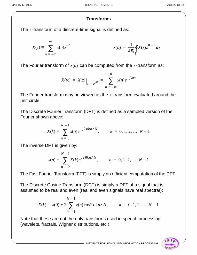
Transforms
The -transform of a discrete-time signal is defined as:
The Fourier transform of can be computed from the -transform as:
The Fourier transform may be viewed as the -transform evaluated around theunit circle.
The Discrete Fourier Transform (DFT) is defined as a sampled version of theFourier shown above:
The inverse DFT is given by:
The Fast Fourier Transform (FFT) is simply an efficient computation of the DFT.
The Discrete Cosine Transform (DCT) is simply a DFT of a signal that isassumed to be real and even (real and even signals have real spectra!):
Note that these are not the only transforms used in speech processing(wavelets, fractals, Wigner distributions, etc.).
z
X z( ) x n( )zn–
n ∞–=
∞
∑≡ x n( )1
2πj-------- X z( )z
n 1–dz
C∫°=
x n( ) z
X ω( ) X z( )z ej ω=
x n( )ejωn–
n ∞–=
∞
∑= =
z
X k( ) x n( )ej2πkn N⁄–
n 0=
N 1–
∑= , k 0 1 2 … N 1–, , , ,=
x n( ) X k( )ej2πkn N⁄
n 0=
N 1–
∑= , n 0 1 2 … N 1–, , , ,=
X k( ) x 0( ) 2 x n( ) 2πkn N⁄cos
n 1=
N 1–
∑+= , k 0 1 2 … N 1–, , , ,=

MAY 15-17, 1996 TEXAS INSTRUMENTS PAGE 23 OF 147
Time-Domain Windowing
Let denote a finite duration segment of a signal:
This introduces frequency domain aliasing (the so-called picket fence effect):
x n( )
x n( ) x n( )w n( )=
0.0 2000.0 4000.0 6000.0 8000.0-40.0
-30.0
-20.0
-10.0
0.0
10.0
20.0
30.0
40.0fs=8000 Hz, f1=1511 Hz, L=25, N=2048
Popular Windows
Generalized Hanning: wH k( ) w k( ) α 1 α–( ) 2πN------k
cos+= 0 α 1< <
α 0.54,= Hamming window
α 0.50,= Hanning window
INSTITUTE FOR SIGNAL AND INFORMATION PROCESSING
Frame-Based Analysis With Overlap
Consider the problem of performing a piecewise linear analysis of a signal:
L L L
x1(n)
x2(n)
x3(n)

INSTITUTE FOR SIGNAL AND INFORMATION PROCESSING
MAY 15-17, 1996 TEXAS INSTRUMENTS PAGE 24 OF 147
Difference Equations, Filters, and Signal Flow Graphs
A linear time-invariant system can be characterized by a constant-coefficientdifference equations:
Is this system linear if the coefficients are time-varying?
Such systems can be implemented as signal flow graphs:
y n( ) aky n k–( )
k 1=
N
∑– bkx n k–( )
k 0=
M
∑+=
y n( )x n( )
+
+
+ +
+
+
+
+
.........
z-1
z-1
z-1
-a1
-aN
-aN-1
-a2
b0
b1
b2
bN-1
bN

INSTITUTE FOR SIGNAL AND INFORMATION PROCESSING
MAY 15-17, 1996 TEXAS INSTRUMENTS PAGE 25 OF 147
Minimum Phase, Maximum Phase, MIxed Phase,and Speech Perception
An FIR filter composed of all zeros that are inside the unit circle is minimumphase. There are many realizations of a system with a given magnitude response;one is a minimum phase realization, one is a maximum-phase realization, othersare in-between. Any non-minimum phase pole-zero system can be decomposedinto:
It can be shown that of all the possible realizations of , the minimum-phaseversion is the most compact in time:Define:
Then, for all and all possible realizations of .
Why is minimum phase such an important concept in speech processing?
We prefer systems that are invertible:
We would like both systems to be stable. The inverse of a non-minimum phasesystem is not stable.
We end with a very simple question:
Is phase important in speech processing?
H z( ) Hmin z( )Hap z( )=
H ω( )
E n( ) h k( )2
k 0=
n
∑=
Emin n( ) E n( )≥ n H ω( )
H z( )H1–
z( ) 1=

INSTITUTE FOR SIGNAL AND INFORMATION PROCESSING
MAY 15-17, 1996 TEXAS INSTRUMENTS PAGE 26 OF 147
Probability Spaces
A formal definition of probability involves the specification of:
• a sample space
The sample space, , is the set of all possible outcomes, plus thenull outcome. Each element in is called a sample point.
• a field (or algebra)
The field, or algebra, is a set of subsets of closed undercomplementation and union (recall Venn diagrams).
• and a probability measure.
A probability measure obeys these axioms:
1. (implies probabilities less than one)2.3. For two mutually exclusive events:
Two events are said to be statistically independent if:
The conditional probability of B given A is:
Hence,
S
S
S
P S( ) 1=
P A( ) 0≥
P A B∪( ) P A B,( ) P A( ) P B( )+= =
P A B∩( ) P A( )P B( )=
P B A( ) P B A∩( )P A( )
----------------------=
P B A∩( ) P B A( )P A( )=
S S
A
BA
B
Mutually ExclusiveP B A∩( ) P B A( )P A( )=

MAY 15-17, 1996 TEXAS INSTRUMENTS PAGE 27 OF 147
Functions of Random Variables
Probability Density Functions:
f(x) - discrete (Histogram)
1 2 3 4
f(x) - continuous
1 2 3 4
Cumulative Distributions:F(x) - discrete F(x) - continuous
INSTITUTE FOR SIGNAL AND INFORMATION PROCESSING
1 2 3 4 1 2 3 4Probability of Events:
f(x) - continuous
1 2 3 4
P 2 x< 3≤( ) f x( ) xd
2
3
∫ F 3( ) F 2( )–= =

INSTITUTE FOR SIGNAL AND INFORMATION PROCESSING
MAY 15-17, 1996 TEXAS INSTRUMENTS PAGE 28 OF 147
Important Probability Density Functions
Uniform (Unix rand function):
Gaussian:
Laplacian (speech signal amplitude, durations):
Gamma (durations):
We can extend these concepts to N-dimensional space. For example:
Two random variables are statistically independent if:
This implies:
and
f x( )1
b a–------------ a x b≤<
0 elsewhere
=
f x( )1
2πσ2----------------- x µ–( )2
–
2σ2-----------------------
exp=
f x( )1
2σ2------------- 2 x–
σ----------------
exp=
f x( )k
2 π x---------------- k x– exp=
P A Ax∈ B Ay∈( ) P A B,( )P B( )
------------------ Ax
∫ f x y,( ) yd xd
Ay
∫
f y( ) yd
Ay
∫-------------------------------------------= =
P A B,( ) P A( )P B( )=
f xy x y,( ) f x x( ) f y y( )= Fxy x y,( ) Fx x( )Fy y( )=

MAY 15-17, 1996 TEXAS INSTRUMENTS PAGE 29 OF 147
Mixture Distributions
A simple way to form a more generalizable pdf that still obeys some para-metric shape is to use a weighted sum of one or more pdfs. We refer to thisas a mixture distribution.
If we start with a Gaussian pdf:
The most common form is a Gaussian mixture:
where
Obviously this can be generalized to other shapes.
Such distributions are useful to accommodate multimodal behavior:
f i x( )1
2πσi2
-------------------x µi–( )2
–
2σi2
------------------------
exp=
f x( ) ci f i x( )
i 1=
N
∑=
cii 1=
N
∑ 1=
1 2 3 4-1-2-3-4
f 1 x( )f 2 x( )
f 3 x( )
µ1 µ2 µ3
Derivation of the optimal coefficients, however, is most often a nonlinearoptimization problem.
INSTITUTE FOR SIGNAL AND INFORMATION PROCESSING

INSTITUTE FOR SIGNAL AND INFORMATION PROCESSING
MAY 15-17, 1996 TEXAS INSTRUMENTS PAGE 30 OF 147
Expectations and Moments
The statistical average of a scalar function, , of a random variable is:
and
The central moment is defined as:
The joint central moment between two random variables is defined as:
We can define a correlation coefficient between two random variables as:
We can extend these concepts to a vector of random variables:
What is the difference between a random vector and a random process?
What does wide sense stationary mean? strict sense stationary?
What does it mean to have an ergodic random process?
How does this influence our signal processing algorithms?
g x( )
E g x( )[ ] xiP x xi=( )
i 1=
∞
∑= E g x( )[ ] g x( ) f x( ) xd
∞–
∞
∫≡
E x µ–( )i[ ] x µ–( )if x( ) xd
∞–
∞
∫=
E x µx–( )iy µy–( )k[ ] x µi–( )i
∞–
∞
∫ y µy–( )kf x y,( ) xd yd
∞–
∞
∫=
ρxy
cxy
ρxρy------------=
x x1 x2 … xN, , ,[ ]T=
f x x( )1
2πN 2⁄ C------------------------------ 1
2---– x µ–( )T
Cx1–
x µ–( )
exp=

INSTITUTE FOR SIGNAL AND INFORMATION PROCESSING
MAY 15-17, 1996 TEXAS INSTRUMENTS PAGE 31 OF 147
Correlation and Covariance of WSS Random Processes
For a signal, , we can compute the following useful quantities:
Autocovariance:
If a random process is wide sense stationary:
Hence, we define a very useful function known as the autocorrelation:
If is zero mean WSS:
What is the relationship between the autocorrelation and the spectrum:
For a linear time-invariant system, :
The notion of random noise is central to signal processing:
white noise?
Gaussian white noise?
zero-mean Gaussian white noise?
colored noise?
Therefore, we now embark upon one of the last great mysteries of life:
How do we compare two random vectors?
x n( )
c i j,( ) E x n i–( ) µi–( ) x n j–( ) µ j–( )[ ]=
E x n i–( )x n j–( )[ ] µiµ j–=
1N---- x n i–( )x n j–( )
n 0=
N 1–
∑ 1N---- x n i–( )
n 0=
N 1–
∑ 1
N---- x n j–( )
n 0=
N 1–
∑
–=
c i j,( ) c i j– 0,( )=
r k( )1N---- x n( )x n k–( )
n 0=
N 1–
∑=
x n( )
c i j,( ) r i j–( )=
DFT r k( ) X k( ) 2=
h n( )
DFT ry k( ) DFT h n( ) 2DFT rx k( ) =

INSTITUTE FOR SIGNAL AND INFORMATION PROCESSING
MAY 15-17, 1996 TEXAS INSTRUMENTS PAGE 32 OF 147
Distance Measures
What is the distance between pt. a and pt. b?
The N-dimensional real Cartesian space,
denoted is the collection of all N-dimensionalvectors with real elements. A metric, or distancemeasure, is a real-valued function with three properties:
:
1. .
2.
3.
The Minkowski metric of order , or the metric, between and is:
(the norm of the difference vector).
Important cases are:1. or city block metric (sum of absolute values),
2. , or Euclidean metric (mean-squared error),
3. or Chebyshev metric,
ℜN
x y z, ,∀ ℜN∈
d x y,( ) 0≥
d x y,( ) 0= if and only if x y=
d x y,( ) d x z,( ) d z y,( )+≤
s ls x y
ds x y,( ) xk yk–s
k 1=
N
∑s≡ x y– s=
l1
d1 x y,( ) xk yk–
k 1=
N
∑=
l2
d2 x y,( ) xk yk–2
k 1=
N
∑=
l∞
d∞ x y,( ) maxk
xk yk–=
0
1
2
0 1 2
gold bars
diamonds
b
a

INSTITUTE FOR SIGNAL AND INFORMATION PROCESSING
MAY 15-17, 1996 TEXAS INSTRUMENTS PAGE 33 OF 147
We can similarly define a weighted Euclidean distance metric:
where:
, , and .
Why are Euclidean distances so popular?
One reason is efficient computation. Suppose we are given a set ofreference vectors, , a measurement, , and we want to find the nearest
neighbor:
This can be simplified as follows:
We note the minimum of a square root is the same as the minimum of asquare (both are monotonically increasing functions):
Therefore,
Thus, a Euclidean distance is virtually equivalent to a dot product (whichcan be computed very quickly on a vector processor). In fact, if all referencevectors have the same magnitude, can be ignored (normalized
codebook).
d2w x y,( ) x y–T
W x y–=
x
x1
x2
…xk
= y
y1
y2
…yk
= W
w11 w12 … w1k
w21 w22 … w2k
… … … …wk1 wk2 … wkk
=
M
xm y
NN minm
d2 xm y,( )=
d2 xm y,( )2
xmjyj–( )2
j 1=
k
∑ xmj
22xmj
yj– yj2
+
j 1=
k
∑= =
xm2
2xm y•– y2
+=
Cm Cy 2xm y•–+=
NN minm
d2 xm y,( ) Cm 2xm y•–= =
Cm

INSTITUTE FOR SIGNAL AND INFORMATION PROCESSING
MAY 15-17, 1996 TEXAS INSTRUMENTS PAGE 34 OF 147
Prewhitening of Features
Consider the problem of comparing features of different scales:
Suppose we represent these points in space in two coordinate systemsusing the transformation:
System 1:
and
System 2:
and
The magnitude of the distance has changed. Though the rank-ordering ofdistances under such linear transformations won’t change, the cumulativeeffects of such changes in distances can be damaging in patternrecognition. Why?
z V x=
β1 1i 0 j+= β2 0i 1 j+=
a 1 0
0 1
1
1= b 1 0
0 1
1
2=
d2 a b,( ) 02
12
+ 1= =
γ1 2– i 0 j+= γ1 1– i 1 j+=
a 2– 0
1– 1
1–
1= b 2– 0
1– 1
32---–
2
=
d2 a b,( ) 1– 32---–
– 2
1 2–( )2+ 5
4---= =
0
1
2
0 1 2
gold bars
diamonds
b
a
System 1
System 2

INSTITUTE FOR SIGNAL AND INFORMATION PROCESSING
MAY 15-17, 1996 TEXAS INSTRUMENTS PAGE 35 OF 147
We can simplify the distance calculation in the transformed space:
This is just a weighted Euclidean distance.
Suppose all dimensions of the vector are not equal in importance. Forexample, suppose one dimension has virtually no variation, while another isvery reliable. Suppose two dimensions are statistically correlated. What is astatistically optimal transformation?
Consider a decomposition of the covariance matrix (which is symmetric):
where denotes a matrix of eigenvectors of and denotes a diagonal
matrix whose elements are the eigenvalues of . Consider:
The covariance of , is easily shown to be an identity matrix (prove this!)
We can also show that:
Again, just a weighted Euclidean distance.
• If the covariance matrix of the transformed vector is a diagonal matrix,the transformation is said to be an orthogonal transform.
• If the covariance matrix is an identity matrix, the transform is said to bean orthonormal transform.
• A common approximation to this procedure is to assume the dimensionsof are uncorrelated but of unequal variances, and to approximate by
a diagonal matrix, . Why? This is known as variance-weighting.
d2 V x V y,( ) V x V y–[ ]TV x V y–[ ]=
x y–[ ]TV
TV x y–[ ]=
d2W x y,( )=
C ΦΛΦT=
Φ C ΛC
z Λ 1 2⁄– Φx=
z Cz
d2 z1 z2,( ) x1 x2–[ ]TCx
1–x1 x2–[ ]=
x C
Λ

INSTITUTE FOR SIGNAL AND INFORMATION PROCESSING
MAY 15-17, 1996 TEXAS INSTRUMENTS PAGE 36 OF 147
“Noise-Reduction”
The prewhitening transform, , is normally created as amatrix in which the eigenvalues are ordered from largest to smallest:
where
.
In this case, a new feature vector can be formed by truncating thetransformation matrix to rows. This is essentially discarding the leastimportant features.
A measure of the amount of discriminatory power contained in a feature, ora set of features, can be defined as follows:
This is the percent of the variance accounted for by the first features.
Similarly, the coefficients of the eigenvectors tell us which dimensions of theinput feature vector contribute most heavily to a dimension of the outputfeature vector. This is useful in determining the “meaning” of a particularfeature (for example, the first decorrelated feature often is correlated withthe overall spectral slope in a speech recognition system — this issometimes an indication of the type of microphone).
z Λ 1 2⁄– Φx= k k×
z1
z2
…zk
λ11 2⁄–
λ21 2⁄–
…
λk1 2⁄–
v11 v12 … v13
v21 v22 … v2k
… … … …vk1 vk2 … vkk
x1
x2
…xk
=
λ1 λ2 … λk> > >
l k<
% var
λ jj 1=
l
∑
λ jj 1=
k
∑-----------------=
l

INSTITUTE FOR SIGNAL AND INFORMATION PROCESSING
MAY 15-17, 1996 TEXAS INSTRUMENTS PAGE 37 OF 147
Computational Procedures
Computing a “noise-free” covariance matrix is often difficult. One mightattempt to do something simple, such as:
and
On paper, this appears reasonable. However, often, the complete set offeature vectors contains valid data (speech signals) and noise (nonspeechsignals). Hence, we will often compute the covariance matrix across asubset of the data, such as the particular acoustic event (a phoneme orword) we are interested in.
Second, the covariance matrix is often ill-conditioned. Stabilizationprocedures are used in which the elements of the covariance matrix arelimited by some minimum value (a noise-floor or minimum SNR) so that thecovariance matrix is better conditioned.
But how do we compute eigenvalues and eigenvectors on a computer?One of the hardest things to do numerically! Why?
Suggestion: use a canned routine (see Numerical Recipes in C).
The definitive source is EISPACK (originally implemented in Fortran, nowavailable in C). A simple method for symmetric matrices is known as theJacobi transformation. In this method, a sequence of transformations areapplied that set one off-diagonal element to zero at a time. The product ofthe subsequent transformations is the eigenvector matrix.
Another method, known as the QR decomposition, factors the covariancematrix into a series of transformations:
where is orthogonal and is upper diagonal. This is based on a
transformation known as the Householder transform that reduces columnsof a matrix below the diagonal to zero.
cij xi µi–( ) xj µ j–( )n 0=
N 1–
∑= µi xin 0=
N 1–
∑=
C QR=
Q R

MAY 15-17, 1996 TEXAS INSTRUMENTS PAGE 38 OF 147
Maximum Likelihood Classification
Consider the problem of assigning a measurement to one of two sets:
µ1 µ2x
f x c x c 1=( )( ) f x c x c 2=( )( )
x
What is the best criterion for making a decision?
Ideally, we would select the class for which the conditional probability is highest:
However, we can’t estimate this probability directly from the training data. Hence,we consider:
By definition
and
from which we have
c∗ argmaxc
= P c c=( ) x x=( )( )
c∗ argmaxc
= P x x=( ) c c=( )( )
P c c=( ) x x=( )( ) P c c=( ) x x=( ),( )
P x x=( )---------------------------------------------=
P x x=( ) c c=( )( ) P c c=( ) x x=( ),( )P c c=( )
---------------------------------------------=
P c c=( ) x x=( )( )P x x=( ) c c=( )( )P c c=( )
P x x=( )------------------------------------------------------------------=
INSTITUTE FOR SIGNAL AND INFORMATION PROCESSING

INSTITUTE FOR SIGNAL AND INFORMATION PROCESSING
MAY 15-17, 1996 TEXAS INSTRUMENTS PAGE 39 OF 147
Clearly, the choice of that maximizes the right side also maximizes the left side.Therefore,
if the class probabilities are equal,
A quantity related to the probability of an event which is used to make a decisionabout the occurrence of that event is often called a likelihood measure.
A decision rule that maximizes a likelihood is called a maximum likelihooddecision.
In a case where the number of outcomes is not finite, we can use an analogouscontinuous distribution. It is common to assume a multivariate Gaussiandistribution:
We can elect to maximize the log, rather than the likelihood (we refer
to this as the log likelihood). This gives the decision rule:
(Note that the maximization became a minimization.)
We can define a distance measure based on this as:
c
c∗ argmaxc
P x x=( ) c c=( )( )[ ]=
argmxc
P x x=( ) c c=( )( )P c c=( )[ ]=
c∗ argmxc
P x x=( ) c c=( )( )[ ]=
f x c x1 … xN,, c( ) f x c x c( )=
1
2π Cx c
------------------------- 12---– x µx c–( )
TCx c
1–x µ
x c–( )
exp=
f x c x c( )[ ]ln
c∗ argminc
x µx c–( )T
Cx c1–
x µx c
–( ) Cx c1–
ln+=
dml x µx c,( ) x µx c–( )T
Cx c1–
x µx c
–( ) Cx c1–
ln+=

MAY 15-17, 1996 TEXAS INSTRUMENTS PAGE 40 OF 147
Note that the distance is conditioned on each class mean and covariance.This is why “generic” distance comparisons are a joke.
If the mean and covariance are the same across all classes, this expressionsimplifies to:
This is frequently called the Mahalanobis distance. But this is nothing morethan a weighted Euclidean distance.
This result has a relatively simple geometric interpretation for the case of asingle random variable with classes of equal variances:
dM x µx c,( ) x µx c–( )T
Cx c1–
x µx c
–( )=
µ1 µ2x
f x c x c 1=( )( ) f x c x c 2=( )( )
a
The decision rule involves setting a threshold:
and,
If the variances are not equal, the threshold shifts towards the distributionwith the smaller variance.
What is an example of an application where the classes are notequiprobable?
aµ1 µ2+
2------------------
σ2
µ1 µ2–------------------ P c 2=( )
P c 1=( )---------------------
ln+=
if x a< x c 1=( )∈else x c 2=( )∈
INSTITUTE FOR SIGNAL AND INFORMATION PROCESSING

INSTITUTE FOR SIGNAL AND INFORMATION PROCESSING
MAY 15-17, 1996 TEXAS INSTRUMENTS PAGE 41 OF 147
Probabilistic Distance Measures
How do we compare two probability distributions to measure their overlap?
Probabilistic distance measures take the form:
where1. is nonnegative2. J attains a maximum when all classes are disjoint3. J=0 when all classes are equiprobable
Two important examples of such measures are:
(1) Bhattacharyya distance:
(2) Divergence
Both reduce to a Mahalanobis-like distance for the case of Gaussian vectorswith equal class covariances.
Such metrics will be important when we attempt to cluster feature vectorsand acoustic models.
J g fx c x c( ) P c c=( ) c 1 2 … K, , ,=,, xd
∞–
∞
∫=
J
JB f x c x 1( ) f x c x 2( ) xd
∞–
∞
∫ln–=
JD f x c x 1( ) f x c x 2( )–[ ]f x c x 1( )
f x c x 2( )----------------------ln xd
∞–
∞
∫=

INSTITUTE FOR SIGNAL AND INFORMATION PROCESSING
MAY 15-17, 1996 TEXAS INSTRUMENTS PAGE 42 OF 147
Probabilistic Dependence Measures
A probabilistic dependence measure indicates how strongly a feature isassociated with its class assignment. When features are independent oftheir class assignment, the class conditional pdf’s are identical to themixture pdf:
When their is a strong dependence, the conditional distribution should besignificantly different than the mixture. Such measures take the form:
An example of such a measure is the average mutual information:
The discrete version of this is:
Mutual information is closely related to entropy, as we shall see shortly.
Such distance measures can be used to cluster data and generate vectorquantization codebooks. A simple and intuitive algorithms is known as theK-means algorithm:
Initialization: Choose K centroids
Recursion: 1. Assign all vectors to their nearest neighbor.
2. Recompute the centroids as the average of all vectorsassigned to the same centroid.
3. Check the overall distortion. Return to step 1 if somedistortion criterion is not met.
f x c x c( ) f x x( )= c∀
J g fx c x c( ) f x x( ) P c c=( ) c 1 2 … K, , ,=,,, xd
∞–
∞
∫=
Mavg c x,( ) P c c=( )
c 1=
K
∑ … f x c x c( )f x c x c( )
f x x( )----------------------log xd
∞–
∞
∫∞–
∞
∫=
Mavg c x,( ) P c c=( )
c 1=
K
∑ P x xl=( )P x xl= c c=( )
P x xl=( )-------------------------------------
2log
i 1=
L
∑=

MAY 15-17, 1996 TEXAS INSTRUMENTS PAGE 43 OF 147
1
1
What Is Information? (When not to bet at a casino...)
Consider two distributions of discrete random variables:
41 2 3 x
c=1 c=2 c=3 c=4
f(x)
Uniform Random Variable
1/4
41 2 3 y
c=1 c=2
c=3
c=4
f(y)
1/2
3/4
/4
/2
3/4
Which variable is more unpredictable?
Now, consider sampling random numbers from a random number generatorwhose statistics are not known. The more numbers we draw, the more wediscover about the underlying distribution. Assuming the underlying distribution isfrom one of the above distributions, how much more information do we receivewith each new number we draw?
The answer lies in the shape of the distributions. For the random variable x, eachclass is equally likely. Each new number we draw provides the maximum amountof information, because, on the average, it will be from a different class (so wediscover a new class with every number). On the other hand, for y, chances are,c=3 will occur 5 times more often than the other classes, so each new sample willnot provide as much information.
We can define the information associated with each class, or outcome, as:
Since , information is a positive quantity. A base 2 logarithm is used so
that discrete outcomes can be measured in bits. For the distributionsabove,
Huh??? Does this make sense?
I c c=( ) 1P c c=( )--------------------
2log≡ P c c=( )2log–=
0 P x( ) 1≤ ≤
K 2M
K=
I x c 1=( ) 1–( ) 1 4⁄( )2log 2 bits= = I y c 1=( ) 1–( ) 18---
2
log 3 bits= =
INSTITUTE FOR SIGNAL AND INFORMATION PROCESSING
INSTITUTE FOR SIGNAL AND INFORMATION PROCESSING
MAY 15-17, 1996 TEXAS INSTRUMENTS PAGE 44 OF 147
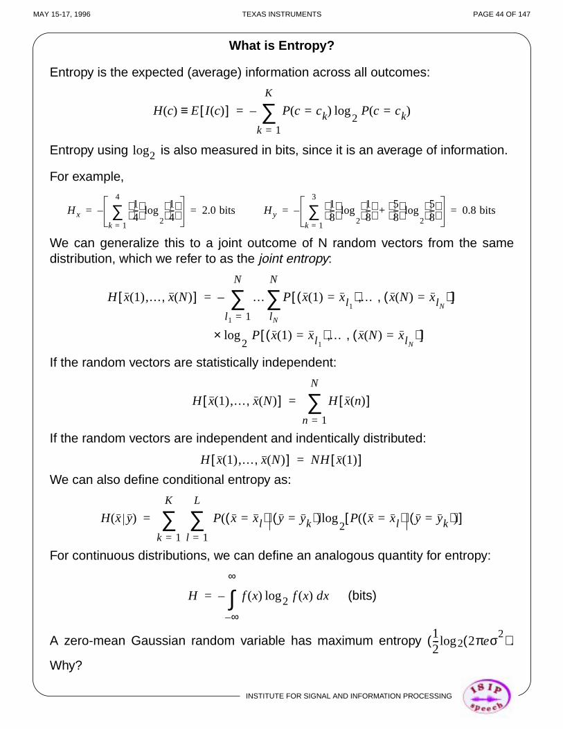
What is Entropy?
Entropy is the expected (average) information across all outcomes:
Entropy using is also measured in bits, since it is an average of information.
For example,
We can generalize this to a joint outcome of N random vectors from the samedistribution, which we refer to as the joint entropy:
If the random vectors are statistically independent:
If the random vectors are independent and indentically distributed:
We can also define conditional entropy as:
For continuous distributions, we can define an analogous quantity for entropy:
(bits)
A zero-mean Gaussian random variable has maximum entropy ( .
Why?
H c( ) E I c( )[ ]≡ P c ck=( ) P c ck=( )2
log
k 1=
K
∑–=
log2
Hx14---
14---
2
logk 1=
4
∑– 2.0 bits= = Hy18---
18---
2
logk 1=
3
∑ 58---
58---
2
log+– 0.8 bits= =
H x 1( ) … x N( ),,[ ] …l1 1=
N
∑ P x 1( ) xl1=( ) … x N( ) xlN
=( ), ,[ ]l N
N
∑–=
P x 1( ) xl1=( ) … x N( ) xlN
=( ), ,[ ]2
log×
H x 1( ) … x N( ),,[ ] H x n( )[ ]n 1=
N
∑=
H x 1( ) … x N( ),,[ ] NH x 1( )[ ]=
H x y( ) P x xl=( ) y yk=( )( ) P x xl=( ) y yk=( )( )[ ]2
log
l 1=
L
∑k 1=
K
∑=
H f x( ) f x( )2log xd
∞–
∞
∫–=
12--- 2πeσ2( )2log

INSTITUTE FOR SIGNAL AND INFORMATION PROCESSING
MAY 15-17, 1996 TEXAS INSTRUMENTS PAGE 45 OF 147
Mutual Information
The pairing of random vectors produces less information than the eventstaken individually. Stated formally:
The shared information between these events is called the mutualinformation, and is defined as:
From this definition, we note:
This emphasizes the idea that this is information shared between these tworandom variables.
We can define the average mutual information as the expectation of themutual information:
Note that:
Also note that if and are independent, then there is no mutualinformation between them.
Note that to compute mutual information between two random variables, weneed a joint probability density function.
I x y,( ) I x( ) I y( )+≤
M x y,( ) I x( ) I y( )+[ ] I x y,( )–≡
M x y,( )P x y,( )
P x( )P y( )---------------------
2log=
1P x( )----------
2log
1P x y,( )P y( )
--------------------------------
2log+=
1P x( )----------
2log
1P x y( )---------------
2log–=
I x( ) I x y( )–=
I y( ) I y x( )–=
M x y,( ) EP x y,( )
P x( )P y( )---------------------
2
log=
P x xl=( ) y yk=( ),( )P x xl=( ) y yk=( ),( )
P x xl=( )P y yk=( )--------------------------------------------------
2log
l 1=
L
∑k 1=
K
∑=
M x y,( ) H x( ) H x y( )– H y x( ) H y( )–= =
x y

MAY 15-17, 1996 TEXAS INSTRUMENTS PAGE 46 OF 147
How Does Entropy Relate To DSP?
Consider a window of a signal:
x(n)
n
window
What does the sampled z-transform assume about the signal outside thewindow?
What does the DFT assume about the signal outside the window?
How do these influence the resulting spectrum that is computed?
What other assumptions could we make about the signal outside thewindow? How many valid signals are there?
How about finding the spectrum that corresponds to the signal that matchesthe measured signal within the window, and has maximum entropy?
What does this imply about the signal outside the window?
This is known as the principle of maximum entropy spectral estimation.Later we will see how this relates to minimizing the mean-square error.
INSTITUTE FOR SIGNAL AND INFORMATION PROCESSING

INSTITUTE FOR SIGNAL AND INFORMATION PROCESSING
MAY 15-17, 1996 TEXAS INSTRUMENTS PAGE 47 OF 147
Session III:
Signal Measurements

INSTITUTE FOR SIGNAL AND INFORMATION PROCESSING
MAY 15-17, 1996 TEXAS INSTRUMENTS PAGE 48 OF 147
Short-Term Measurements
What is the point of this lecture?
T f 5 ms=
Tw 10 ms=
T f 10 ms=
Tw 20 ms=
T f 20 ms=
Tw 30 ms=
T f 20 ms=
Tw 30 ms=
Hamm. Win.
T f 20 ms=
Tw 60 ms=
Hamm. Win.
Speech Signal
Recursive50 Hz LPF

INSTITUTE FOR SIGNAL AND INFORMATION PROCESSING
MAY 15-17, 1996 TEXAS INSTRUMENTS PAGE 49 OF 147
Time/Frequency Properties of Windows
%OverlapTw T f–( )
Tw------------------------- 100%×=
• Generalized Hanning: wH k( ) w k( ) α 1 α–( ) 2πN------k
cos+= 0 α 1< <
α 0.54,= Hamming window
α 0.50,= Hanning window

INSTITUTE FOR SIGNAL AND INFORMATION PROCESSING
MAY 15-17, 1996 TEXAS INSTRUMENTS PAGE 50 OF 147
Recursive-in-Time Approaches
Define the short-term estimate of the power as:
We can view the above operation as a moving-average filter applied to the
sequence .
This can be computed recursively using a linear constant-coefficientdifference equation:
Common forms of this general equation are:
(Leaky Integrator)
(First-order weighted average)
(2nd-order Integrator)
Of course, these are nothing more than various types of low-pass filters, oradaptive controllers. How do we compute the constants for theseequations?
In what other applications have we seen such filters?
P n( )1
Ns------ w m( )s n
Ns
2------ m+–( )
2
m 0=
Ns 1–
∑=
s2
n( )
P n( ) apw i( )P n i–( )
i 1=
Na
∑– bpw j( )s2
n j–( )
j 1=
Nb
∑+=
P n( ) αP n 1–( ) s2
n( )+=
P n( ) αP n 1–( ) 1 α–( )s2n( )+=
P n( ) αP n 1–( ) βP n 2–( ) s2
n( ) γ s2
n 1–( )+ + +=

MAY 15-17, 1996 TEXAS INSTRUMENTS PAGE 51 OF 147
Relationship to Control Systems
The first-order systems can be related to physical quantities by observingthat the system consists of one real pole:
can be defined in terms of the bandwidth of the pole.
For second-order systems, we have a number of alternatives. Recall that asecond-order system can consist of at most one zero and one pole and theircomplex conjugates. Classical filter design algorithms can be used to designthe filter in terms of a bandwidth and an attenuation.
An alternate approach is to design the system in terms of its unit-stepresponse:
H z( ) 1
1 αz1–
–---------------------=
α
u(n)
P(n)
n
Overshoot
rise times
1.0
0.5
0settling time
final response threshold
h(n)
n
Equivalent impulse responserise time
fall time
There are many forms of such controllers (often known asservo-controllers). One very interesting family of such systems are thosethat correct to the velocity and acceleration of the input. All such systemscan be implemented as a digital filter.
INSTITUTE FOR SIGNAL AND INFORMATION PROCESSING

MAY 15-17, 1996 TEXAS INSTRUMENTS PAGE 52 OF 147
Short-Term Autocorrelation and Covariance
Recall our definition of the autocorrelation function:
Note:
• this can be regarded as a dot product of and .• let’s not forget preemphasis, windowing, and centering the window
w.r.t. the frame, and that scaling is optional.What would C++ code look like:
r k( )1N---- s n( )s n k–( )
n k=
N 1–
∑ 1N---- s n( )s n k+( )
n 0=
N 1– k–
∑= = 0 k p< <
s n( ) s n i+( )
array-style:for(k=0; k<M; k++)
r[k] = 0.0;for(n=0; n<N-k; n++)
r[k] += s[n] * s[n+k]
pointer-style:for(k=0; k<M; k++)
*r = 0.0; s = sig; sk = sig + k;for(n=0; n<N-i; n++)
*r += (s++) * (sk++);
We note that we can save some multiplications by reusing products:
This is known as the factored autocorrelation computation.It saves about 25% CPU, replacing multiplications with additions and morecomplicated indexing.
Similarly, recall our definition of the covariance function:
Note:• we use N-p points
• symmetric so that only the terms need to be computed
This can be simplified using the recursion:
r 3[ ] s 3[ ] s 0[ ] s 6[ ]+( ) s 4[ ] s 1[ ] s 7[ ]+( ) … s N[ ]s N 3–[ ]+ + +=
c k l,( )1N---- s n k–( )s n l–( )
n p=
N 1–
∑= 0 l k p< < <
k l≥
c k l,( ) c k 1– l 1–,( ) s p k–( )s p l–( ) s N k–( )s N l–( )–+=
INSTITUTE FOR SIGNAL AND INFORMATION PROCESSING

INSTITUTE FOR SIGNAL AND INFORMATION PROCESSING
MAY 15-17, 1996 TEXAS INSTRUMENTS PAGE 53 OF 147
Example of the Autocorrelation Function
Autocorrelation functions for the word “three” comparing the consonantportion of the waveform to the vowel (256-point Hamming window).
Note:• shape for the low order lags - what does this correspond to?• regularity of peaks for the vowel — why?• exponentially-decaying shape — which harmonic?• what does a negative correlation value mean?

MAY 15-17, 1996 TEXAS INSTRUMENTS PAGE 54 OF 147
An Application of Short-Term Power: Speech SNR Measurement
Problem: Can we estimate the SNR from a speech file?
0.0 10.0 20.0 30.0-10000.0
-5000.0
0.0
5000.0
10000.0
Energy Histogram:
E
p(E)
Cumulative Distribution:
E
cdf(E)
Nominal Signal+Noise Level
80%
Nominal Noise Level
20%
100% by definition
The SNR can defined as:
What percentiles to use?
Typically, 80%/20%, 85%/15%, or 95%/15% are used.
SNR 10Es
En------
10log 10
Es En+( ) En–
En------------------------------------
10log= =
INSTITUTE FOR SIGNAL AND INFORMATION PROCESSING

INSTITUTE FOR SIGNAL AND INFORMATION PROCESSING
MAY 15-17, 1996 TEXAS INSTRUMENTS PAGE 55 OF 147
Linear Prediction (General)
Let us define a speech signal, , and a predicted value: .
Why the added terms? This prediction error is given by:
We would like to minimize the error by finding the best, or optimal, value of .
Let us define the short-time average prediction error:
We can minimize the error w.r.t for each by differentiating and
setting the result equal to zero:
s n( ) s n( ) αks n k–( )
k 1=
p
∑=
e n( ) s n( ) s n( )– s n( ) αks n k–( )
k 1=
p
∑–= =
αk
E e2
n( )n∑=
s n( ) αks n k–( )
k 1=
p
∑–
2
n∑=
s2
n( )n∑ 2s n( ) αks n k–( )
k 1=
p
∑
n∑– αks n k–( )
k 1=
p
∑ 2
n∑+=
s2
n( )n∑ 2 αk s n( )s n k–( )
n∑
k 1=
p
∑– αks n k–( )
k 1=
p
∑ 2
n∑+=
αl 1 l p≤ ≤ E
αl∂∂E 0 2– s n( )s n l–( )
n∑ 2 αks n k–( )
k 1=
p
∑
s n l–( )n∑+= =

INSTITUTE FOR SIGNAL AND INFORMATION PROCESSING
MAY 15-17, 1996 TEXAS INSTRUMENTS PAGE 56 OF 147
Linear Prediction (Cont.)
Rearranging terms:
or,
This equation is known and the linear prediction (Yule-Walker) equation. are known as linear prediction coefficients, or predictor coefficients.
By enumerating the equations for each value of , we can express this inmatrix form:
where,
The solution to this equation involves a matrix inversion:
and is known as the covariance method. Under what conditions doesexist?
Note that the covariance matrix is symmetric. A fast algorithm to find the
solution to this equation is known as the Cholesky decomposition (aapproach in which the covariance matrix is factored into lower and uppertriangular matrices).
s n( )s n l–( )n∑ αk s n k–( )s n l–( )
n∑
k 1=
p
∑=
c l 0,( ) αkc k l,( )
k 1=
p
∑=
αk
l
c Cα=
α
α1
α2
…αp
= C
c 1 1,( ) c 1 2,( ) … c 1 p,( )
c 2 1,( ) c 2 2,( ) … c 2 p,( )
… … … …c p 1,( ) c p 2,( ) … c p p,( )
= c
c 1 0,( )
c 2 0,( )
…c p 0,( )
=
α C1–c=
C1–
V DVT

INSTITUTE FOR SIGNAL AND INFORMATION PROCESSING
MAY 15-17, 1996 TEXAS INSTRUMENTS PAGE 57 OF 147
The Autocorrelation Method
Using a different interpretation of the limits on the error minimization —forcing data only within the frame to be used — we can compute thesolution to the linear prediction equation using the autocorrelation method:
where,
Note that is symmetric, and all of the elements along the diagonal areequal, which means (1) an inverse always exists; (2) the roots are in the left-half plane.
The linear prediction process can be viewed as a filter by noting:
and
where
is called the analyzer; what type of filter is it? (pole/zero? phase?)
is called the synthesizer; under what conditions is it stable?
α R1–r=
α
α1
α2
…αp
= R
r 0( ) r 1( ) … r p 1–( )
r 1( ) r 0( ) … r p 2–( )
… … … …r p 1–( ) r p 2–( ) … r 0( )
= r
r 1( )
r 2( )
…r p( )
=
R
e n( ) s n( ) αks n k–( )
k 1=
p
∑–=
E z( ) S z( )A z( )=
A z( ) 1 αkzk–
k 1=
p
∑–=
A z( )
1A z( )----------

INSTITUTE FOR SIGNAL AND INFORMATION PROCESSING
MAY 15-17, 1996 TEXAS INSTRUMENTS PAGE 58 OF 147
Linear Prediction Error
We can return to our expression for the error:
and substitute our expression for and show that:
Autocorrelation Method:
Covariance Method:
Later, we will discuss the properties of these equations as they relate to themagnitude of the error. For now, note that the same linear predictionequation that applied to the signal applies to the autocorrelation function,except that samples are replaced by the autocorrelation lag (and hence thedelay term is replaced by a lag index).
Since the same coefficients satisfy both equations, this confirms ourhypothesis that this is a model of the minimum-phase version of the inputsignal.
Linear prediction has numerous formulations including the covariancemethod, autocorrelation formulation, lattice method, inverse filterformulation, spectral estimation formulation, maximum likelihoodformulation, and inner product formulation. Discussions are found indisciplines ranging from system identification, econometrics, signalprocessing, probability, statistical mechanics, and operations research.
E e2
n( )n∑ s n( ) αks n k–( )
k 1=
p
∑–
2
n∑= =
αk
E r 0( ) αkr k( )
k 1=
p
∑–=
E c 0 0,( ) αkc 0 k,( )
k 1=
p
∑–=

INSTITUTE FOR SIGNAL AND INFORMATION PROCESSING
MAY 15-17, 1996 TEXAS INSTRUMENTS PAGE 59 OF 147
Levinson-Durbin Recursion
The predictor coefficients can be efficiently computed for the autocorrelationmethod using the Levinson-Durbin recursion:
This recursion gives us great insight into the linear prediction process. First,we note that the intermediate variables, , are referred to as reflection
coefficients.
Example: p=2
This reduces the LP problem to and saves an order of magnitude incomputational complexity, and makes this analysis amenable to fixed-pointdigital signal processors and microprocessors.
for i 1 2 … p, , ,=
E0 r 0( )=
ki r i( ) ai 1– j( )r i j–( )
j 1=
i 1–
∑–
Ei 1–⁄=
for j 1 2 … i 1–, , ,=
ai i( ) ki=
ai j( ) ai 1– j( ) kiai 1– i j–( )–=
Ei 1 ki2
–( )Ei 1–=
ki
E0 r 0( )=
k1 r 1( ) r 0( )⁄=
a1 1( ) k1 r 1( ) r 0( )⁄= =
E1 1 k12
–( )E0=
r2
0( ) r2
1( )–r 0( )
------------------------------=
k2r 2( )r 0( ) r
21( )–
r2
0( ) r2
1( )–-------------------------------------=
a2 2( ) k2r 2( )r 0( ) r
21( )–
r2
0( ) r2
1( )–-------------------------------------= =
a2 1( ) a1 1( ) k2a1 1( )–=
r 1( )r 0( ) r 1( )r 2( )–
r2
0( ) r2
1( )–--------------------------------------------=
α1 a2 1( )=
α2 a2 2( )=
O p( )

INSTITUTE FOR SIGNAL AND INFORMATION PROCESSING
MAY 15-17, 1996 TEXAS INSTRUMENTS PAGE 60 OF 147
Linear Prediction Coefficient Transformations
The predictor coefficients and reflection coefficients can be transformedback and forth with no loss of information:
Predictor to reflection coefficient transformation:
Reflection to predictor coefficient transformation:
Also, note that these recursions require intermediate storage for .
From the above recursions, it is clear that . In fact, there are several
important results related to :
(1)
(2) , implies a harmonic process (poles on the unit circle).
(3) implies an unstable synthesis filter (poles outside the unit circle).
(4)
This gives us insight into how to determine the LP order during the calcula-tions. We also see that reflection coefficients are orthogonal in the sensethat the best order “p” model is also the first “p” coefficients in the order“p+1” LP model (very important!).
for i p p 1– … 1, , ,=
ki ai i( )=
ai 1– j( )ai j( ) kiai i j–( )+
1 ki2
–----------------------------------------= 1 j i 1–≤ ≤
for i 1 2 … p, , ,=
ai i( ) ki=
ai j( ) ai 1– j( ) kiai 1– i j–( )–= 1 j i 1–≤ ≤
ai
ki 1≠
ki
ki 1<
ki 1=
ki 1>
E0 E1 … Ep> > >
INSTITUTE FOR SIGNAL AND INFORMATION PROCESSING
MAY 15-17, 1996 TEXAS INSTRUMENTS PAGE 61 OF 147
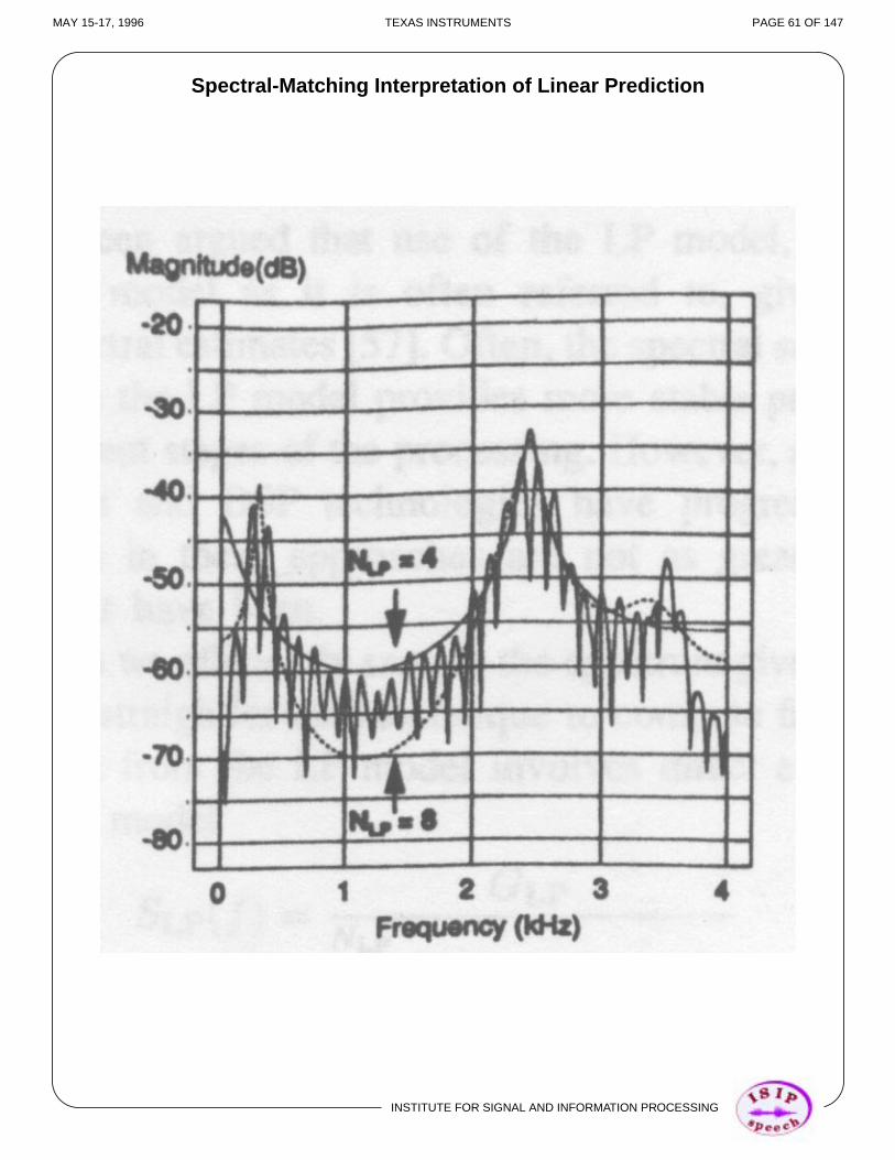
Spectral-Matching Interpretation of Linear Prediction

INSTITUTE FOR SIGNAL AND INFORMATION PROCESSING
MAY 15-17, 1996 TEXAS INSTRUMENTS PAGE 62 OF 147
Noise-Weighting

INSTITUTE FOR SIGNAL AND INFORMATION PROCESSING
MAY 15-17, 1996 TEXAS INSTRUMENTS PAGE 63 OF 147
The Real Cepstrum
Goal: Deconvolve spectrum for multiplicative processes
In practice, we use the “real” cepstrum:
and manifest themselves at the low and high end of the “quefrency”domain respectively.
We can derive cepstral parameters directly from LP analysis:
To obtain the relationship between cepstral and predictor coefficients, we can
differentiate both sides is taken with respect to :
which simplifies to
Note that the order of the cepstral coefficients need not be the same as the orderof the LP model. Typically, 10-16 LP coefficients are used to generate 10-12cepstral coefficients.
Cs ω( ) S f( )log=
V f( )U f( )log=
V f( )log U f( )log+=
V f( ) U f( )
A z( )ln C z( ) cnzn–
n 1=
∞
∑= =
z1–
z1–
d
dA z( )ln
z1–
d
d 1
1 αkzk–
k 1=
p
∑–
-----------------------------------ln
z1–
d
dcnz
n–
n 1=
∞
∑= =
c1 a1=
cn 1 k n⁄–( )αkcn k– an+
k 1=
n 1–
∑=

INSTITUTE FOR SIGNAL AND INFORMATION PROCESSING
MAY 15-17, 1996 TEXAS INSTRUMENTS PAGE 64 OF 147
Session IV:
Signal Processing
In Speech Recognition

INSTITUTE FOR SIGNAL AND INFORMATION PROCESSING
MAY 15-17, 1996 TEXAS INSTRUMENTS PAGE 65 OF 147
THE SIGNAL MODEL (“FRONT-END”)
SpectralModeling
ParametricTransform
SpectralAnalysis
SpectralShaping
Speech
Conditioned Signal
Spectral Measurements
Spectral Parameters
Observation Vectors
Digital Signal Processing
Speech Recognition

INSTITUTE FOR SIGNAL AND INFORMATION PROCESSING
MAY 15-17, 1996 TEXAS INSTRUMENTS PAGE 66 OF 147
A TYPICAL “FRONT-END”
Time-Derivative
CepstralAnalysis
FourierTransform
Signal
mel-spaced cepstral coefficients
secondderivative
firstderivative
(rate of change)
absolutespectral
measurements
energydelta-energy
Time-Derivative

INSTITUTE FOR SIGNAL AND INFORMATION PROCESSING
MAY 15-17, 1996 TEXAS INSTRUMENTS PAGE 67 OF 147
Putting It All Together

INSTITUTE FOR SIGNAL AND INFORMATION PROCESSING
MAY 15-17, 1996 TEXAS INSTRUMENTS PAGE 68 OF 147
Mel Cepstrum
Bark 130.76f1000--------------
atan=
3.5f2
7500)2( )----------------------
atan+
mel f 2595 10 1 f7000------------+
log=
BWcrit 25 75 1 1.4f
1000------------
2+
0.69+=

INSTITUTE FOR SIGNAL AND INFORMATION PROCESSING
MAY 15-17, 1996 TEXAS INSTRUMENTS PAGE 69 OF 147
Mel Cepstrum Computation Via A Filter Bank
Index
Bark Scale Mel Scale
CenterFreq.(Hz)
BW(Hz)
CenterFreq.(Hz)
BW(Hz)
1 50 100 100 100
2 150 100 200 100
3 250 100 300 100
4 350 100 400 100
5 450 110 500 100
6 570 120 600 100
7 700 140 700 100
8 840 150 800 100
9 1000 160 900 100
10 1170 190 1000 124
11 1370 210 1149 160
12 1600 240 1320 184
13 1850 280 1516 211
14 2150 320 1741 242
15 2500 380 2000 278
16 2900 450 2297 320
17 3400 550 2639 367
18 4000 700 3031 422
19 4800 900 3482 484
20 5800 1100 4000 556
21 7000 1300 4595 639
22 8500 1800 5278 734
23 10500 2500 6063 843
24 13500 3500 6964 969

INSTITUTE FOR SIGNAL AND INFORMATION PROCESSING
MAY 15-17, 1996 TEXAS INSTRUMENTS PAGE 70 OF 147
Mel Cepstrum ComputationVia
Oversampling Using An FFT
• • •
fi-1 fi
S(f)
frequency
• Note that an FFT yields frequency samples at
• Oversampling provides a smoother estimate of the envelope of the spectrum
• Other analogous techniques efficient sampling techniques exist for differentfrequency scales (bilinear transform, sampled autocorrelation, etc.)
kN----
f s

INSTITUTE FOR SIGNAL AND INFORMATION PROCESSING
MAY 15-17, 1996 TEXAS INSTRUMENTS PAGE 71 OF 147
Perceptual Linear Prediction
Goals: Apply greater weight to perceptually-important portions of the spectrumAvoid uniform weighting across the frequency band
Algorithm:
• Compute the spectrum via a DFT
• Warp the spectrum along the Bark frequency scale
• Convolve the warped spectrum with the power spectrum of the simulatedcritical band masking curve and downsample (to typically 18 spectralsamples)
• Preemphasize by the simulated equal-loudness curve:
• Simulate the nonlinear relationship between intensity and perceivedloudness by performing a cubic-root amplitude compression
• Compute an LP model
Claims:
• Improved speaker independent recognition performance
• Increased robustness to noise, variations in the channel, and microphones

INSTITUTE FOR SIGNAL AND INFORMATION PROCESSING
MAY 15-17, 1996 TEXAS INSTRUMENTS PAGE 72 OF 147
Linear Regression and Parameter Trajectories
Premise: Time differentiation of features is a noisy process
Approach: Fit a polynomial to the data to provide a smooth trajectory for aparameter; use closed-loop estimation of the polynomialcoefficients
Static feature:
Dynamic feature:
Acceleration feature:
We can generalize this using an rth order regression analysis:
where (the number of analysis frames in time length T) is odd,and the orthogonal polynomials are of the form:
This approach has been generalized in such a way that the weights on thecoefficients can be estimated directly from training data to maximize thelikelihood of the estimated feature (maximum likelihood linear regression).
s n( ) ck n( )=
s n( ) ck n ∆+( ) ck n ∆–( )–≈
s n( ) s n ∆+( ) s n ∆–( )–≈
Rrk t T ∆T, ,( )
Pr X L,( )Ck t XL 1+
2------------–
∆T+
X 1=
L
∑
Pr2
X L,( )X 1=
L
∑--------------------------------------------------------------------------------------------=
L T ∆T⁄=
P0 X L,( ) 1=
P1 X L,( ) X=
P2 X L,( ) X2 1
12------ L
21–( )–=
P3 X L,( ) X3 1
20------ 3L
27–( )X–=

INSTITUTE FOR SIGNAL AND INFORMATION PROCESSING
MAY 15-17, 1996 TEXAS INSTRUMENTS PAGE 73 OF 147
Session V:
Dynamic Programming

INSTITUTE FOR SIGNAL AND INFORMATION PROCESSING
MAY 15-17, 1996 TEXAS INSTRUMENTS PAGE 74 OF 147

INSTITUTE FOR SIGNAL AND INFORMATION PROCESSING
MAY 15-17, 1996 TEXAS INSTRUMENTS PAGE 75 OF 147
The Principle of Dynamic Programming
• An efficient algorithm for finding the optimal path through a network

INSTITUTE FOR SIGNAL AND INFORMATION PROCESSING
MAY 15-17, 1996 TEXAS INSTRUMENTS PAGE 76 OF 147
Word Spotting ViaRelaxed and Unconstrained Endpointing
• Endpoints, or boundaries, need not be fixed — numerous types ofconstraints can be invoked

INSTITUTE FOR SIGNAL AND INFORMATION PROCESSING
MAY 15-17, 1996 TEXAS INSTRUMENTS PAGE 77 OF 147
Slope Constraints:Increased Efficiency and Improved Performance
• Local constraints used to achieve slope constraints

MAY 15-17, 1996 TEXAS INSTRUMENTS PAGE 78 OF 147
DTW, Syntactic Constraints, and Beam Search
Consider the problem of connected digit recognition: “325 1739”. In thesimplest case, any digit can follow any other digit, but we might know theexact number of digits spoken.
An elegant solution to the problem of finding the best overall sentencehypothesis is known as level building (typically assumes models are samelength.
R1
R2
R3
R4
R5
F1 F5 F10 F15 F20 F25 F30
Possible word endings for first word
Reference
Test
Possible starts for second word
• Though this algorithm is no longer widely used, it gives us a glimpse intothe complexity of the syntactic pattern recognition problem.
INSTITUTE FOR SIGNAL AND INFORMATION PROCESSING

MAY 15-17, 1996 TEXAS INSTRUMENTS PAGE 79 OF 147
R
R
R
R
R
R
Level Building For An Unknown Number Of Words
1
2
3
4
5
F1 F5 F10 F15 F20 F25 F30
eference
Test
Beam
M=5
M=4
M=3
M=2
M=1
• Paths can terminate on any level boundary indicating a different numberof words was recognized (note the significant increase in complexity)
• A search band around the optimal path can be maintained to reduce thesearch space
• Next-best hypothesis can be generated (N-best)• Heuristics can be applied to deal with free endpoints, insertion of silence
between words, etc.• Major weakness is the assumption that all models are the same length!
INSTITUTE FOR SIGNAL AND INFORMATION PROCESSING

INSTITUTE FOR SIGNAL AND INFORMATION PROCESSING
MAY 15-17, 1996 TEXAS INSTRUMENTS PAGE 80 OF 147
The One-Stage Algorithm (“Bridle Algorithm”)
The level building approach is not conducive to models of different lengths,and does not make it easy to include syntactic constraints (which words canfollow previous hypothesized words).
An elegant algorithm to perform this search in one pass is demonstratedbelow:
Reference
Test
R1
R2
R3
Model
• Very close to current state-of-the-art doubly-stochastic algorithms (HMM)• Conceptually simple, but difficult to implement because we must
remember information about the interconnections of hypotheses• Amenable to beam-search concepts and fast-match concepts• Supports syntactic constraints by limited the choices for extending a
hypothesis• Becomes complex when extended to allow arbitrary amounts of silence
between words• How do we train?

INSTITUTE FOR SIGNAL AND INFORMATION PROCESSING
MAY 15-17, 1996 TEXAS INSTRUMENTS PAGE 81 OF 147
Introduction of Syntactic Information
• The search space for vocabularies of hundreds of words can becomeunmanageable if we allow any word to follow any other word (often calledthe no-grammar case)
• Our rudimentary knowledge of language tells us that, in reality, only asmall subset of the vocabulary can follow a given word hypothesis, butthat this subset is sensitive to the given word (we often refer to this as“context-sensitive”)
• In real applications, user-interface design is crucial (much like theproblem of designing GUI’s), and normally results in a specification of alanguage or collection of sentence patterns that are permissible
• A simple way to express and manipulate this information in a dynamicprogramming framework is a via a state machine:
B
C D
Start Stop
E
For example, when you enter state C, you output one of the followingwords: daddy, mommy.If:
state A: givestate B: mestate C: daddy, mommystate D: comestate E: here
We can generate phrases such as:
Daddy give me
• We can represent such information numerous ways (as we shall see)
A

INSTITUTE FOR SIGNAL AND INFORMATION PROCESSING
MAY 15-17, 1996 TEXAS INSTRUMENTS PAGE 82 OF 147
Early Attempts At Introducing Syntactic Information Were “Ad-Hoc”
Feature Extractor
Unconstrained EndpointDynamic Programming
(Word Spotting)
Recognized Sequence of Words (“Sentences”)
P(w2)
P(w1) P(w3)
P(w4)
P(w4)
P(wi)
Finite Automaton
Reference Models
Speech Signal
Measurements

INSTITUTE FOR SIGNAL AND INFORMATION PROCESSING
MAY 15-17, 1996 TEXAS INSTRUMENTS PAGE 83 OF 147
BASIC TECHNOLOGY — A PATTERN RECOGNITION PARADIGMBASED ON
HIDDEN MARKOV MODELS
Search Algorithms:P Wti
Ot( )P Ot Wt
i( )P Wt
i( )
P Ot( )--------------------------------------=
Pattern Matching: Wti
P Ot Ot 1– … Wti, ,( ),[ ]
Signal Model:P Ot Wt 1– Wt Wt 1+, ,( )( )
Recognized Symbols:P S O( ) maxargT
P Wti
Ot Ot 1– …, ,( )( )i
∏=
Language Model:P Wti
( )
Prediction
INSTITUTE FOR SIGNAL AND INFORMATION PROCESSING
MAY 15-17, 1996 TEXAS INSTRUMENTS PAGE 84 OF 147
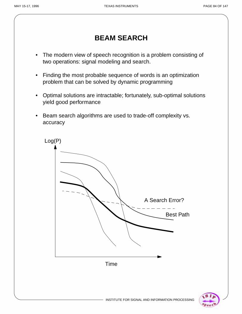
BEAM SEARCH
• The modern view of speech recognition is a problem consisting oftwo operations: signal modeling and search.
• Finding the most probable sequence of words is an optimizationproblem that can be solved by dynamic programming
• Optimal solutions are intractable; fortunately, sub-optimal solutionsyield good performance
• Beam search algorithms are used to trade-off complexity vs.accuracy
Log(P)
Time
Best Path
A Search Error?

INSTITUTE FOR SIGNAL AND INFORMATION PROCESSING
MAY 15-17, 1996 TEXAS INSTRUMENTS PAGE 85 OF 147
Session VI:
Hidden Markov Models

INSTITUTE FOR SIGNAL AND INFORMATION PROCESSING
MAY 15-17, 1996 TEXAS INSTRUMENTS PAGE 86 OF 147
A Simple Markov Model For Weather Prediction
What is a first-order Markov chain?
We consider only those processes for which the right-hand side isindependent of time:
with the following properties:
The above process can be considered observable because the outputprocess is a set of states at each instant of time, where each statecorresponds to an observable event.
Later, we will relax this constraint, and make the output related to the statesby a second random process.
Example: A three-state model of the weather
State 1: precipitation (rain, snow, hail, etc.)State 2: cloudyState 3: sunny
P qt j= qt 1– i= qt 2– k= …, ,( )[ ] P qt j= qt 1– i=[ ]=
aij P qt j= qt 1– i=[ ]= 1 i j, N≤ ≤
aij 0≥ j i,∀
aijj 1=
N
∑ 1= i∀
1 2
3
0.4 0.6
0.3
0.2
0.20.10.1
0.3
0.8

INSTITUTE FOR SIGNAL AND INFORMATION PROCESSING
MAY 15-17, 1996 TEXAS INSTRUMENTS PAGE 87 OF 147
Basic Calculations
Example: What is the probability that the weather for eight consecutivedays is “sun-sun-sun-rain-rain-sun-cloudy-sun”?
Solution:O = sun sun sun rain rain sun cloudy sun
3 3 3 1 1 3 2 3
Example: Given that the system is in a known state, what is the probabilitythat it stays in that state for d days?
O = i i i ... i j
Note the exponential character of this distribution.We can compute the expected number of observations in a state giventhat we started in that state:
Thus, the expected number of consecutive sunny days is (1/(1-0.8)) = 5;the expected number of cloudy days is 2.5, etc.
What have we learned from this example?
P O Model( ) P 3[ ]P 3 3[ ]P 3 3[ ]P 1 3[ ]P 1 1[ ]P 3 1[ ]P 2 3[ ]P 3 2[ ]=
π3a33a31a11a13a32a23=
1.536 104–×=
P O Model q1 i=,( ) P O q1 i=, Model( ) P q1 i=( )⁄=
πiaiid 1–
1 aii–( ) πi⁄=
aiid 1–
1 aii–( )=
pi d( )=
di d pi d( )
d 1=
∞
∑ daiid 1–
1 aii–( )d 1=
∞
∑ 11 aii–---------------= = =

INSTITUTE FOR SIGNAL AND INFORMATION PROCESSING
MAY 15-17, 1996 TEXAS INSTRUMENTS PAGE 88 OF 147
Why Are They Called “Hidden” Markov Models?
Consider the problem of predicting the outcome of a coin toss experiment.You observe the following sequence:
What is a reasonable model of the system?
O HHTTTHTTH…H( )=
1 2
P(H) 1-P(H)
1-P(H)
P(H)
1 2
a11 a221-a11
1-a22
1 2
3
Heads Tails
1-Coin Model(Observable Markov Model)O = H H T T H T H H T T H ...S = 1 1 2 2 1 2 1 1 2 2 1 ...
2-Coins Model(Hidden Markov Model)O = H H T T H T H H T T H ...S = 1 1 2 2 1 2 1 1 2 2 1 ...
P(H) = P1 P(H) = P2
P(T) = 1-P1 P(T) = 1-P2
a11 a22
a12
a21
a13
a31a32
a23
a33
P(H): P1 P2 P3
P(T): 1-P1 1-P2 1-P3
3-Coins Model(Hidden Markov Model)O = H H T T H T H H T T H ...S = 3 1 2 3 3 1 1 2 3 1 3 ...

INSTITUTE FOR SIGNAL AND INFORMATION PROCESSING
MAY 15-17, 1996 TEXAS INSTRUMENTS PAGE 89 OF 147
Why Are They Called Doubly Stochastic Systems?
The Urn-and-Ball Model
P(red) = b1(1)
P(green) = b1(2)
P(blue) = b1(3)
P(yellow) = b1(4)
...
P(red) = b2(1)
P(green) = b2(2)
P(blue) = b2(3)
P(yellow) = b2(4)
...
P(red) = b3(1)
P(green) = b3(2)
P(blue) = b3(3)
P(yellow) = b3(4)
...
O = green, blue, green, yellow, red, ..., blue
How can we determine the appropriate model for the observationsequence given the system above?

INSTITUTE FOR SIGNAL AND INFORMATION PROCESSING
MAY 15-17, 1996 TEXAS INSTRUMENTS PAGE 90 OF 147
Elements of a Hidden Markov Model (HMM)
• N — the number of states
• M — the number of distinct observations per state
• The state-transition probability distribution
• The output probability distribution
• The initial state distribution
We can write this succinctly as:
Note that the probability of being in any state at any time is completelydetermined by knowing the initial state and the transition probabilities:
Two basic problems:
(1) how do we train the system?
(2) how do we estimate the probability of a given sequence(recognition)?
This gives rise to a third problem:
If the states are hidden, how do we know what states were used togenerate a given output?
How do we represent continuous distributions (such as feature vectors)?
A aij =
B bj k( ) =
π πi =
λ A B π, ,( )=
π t( ) At 1– π=

INSTITUTE FOR SIGNAL AND INFORMATION PROCESSING
MAY 15-17, 1996 TEXAS INSTRUMENTS PAGE 91 OF 147
Formalities
The discrete observation HMM is restricted to the production of a finite setof discrete observations (or sequences). The output distribution at any stateis given by:
The observation probabilities are assumed to be independent of time. Wecan write the probability of observing a particular observation, , as:
The observation probability distribution can be represented as a matrixwhose dimension is K rows x S states.We can define the observation probability vector as:
, or,
The mathematical specification of an HMM can be summarized as:
For example, reviewing our coin-toss model:
b k i,( ) P y t( ) k= x t( ) i=( )≡
y t( )
b y t( ) i( ) P y t( ) y t( )= x t( ) i=( )≡
p t( )
P y t( ) 1=( )
P y t( ) 2=( )
…P y t( ) K=( )
= p t( ) Bπ t( ) BAt 1– π 1( )= =
M S π 1( ) A B yk 1 k K≤ ≤, , , , , =
1 2
3
a11 a22
a12
a21
a13
a31a32
a23
a33
P(H): P1 P2 P3
P(T): 1-P1 1-P2 1-P3
S 3=
π 1( )
1 3⁄1 3⁄1 3⁄
=
A
a11 a12 a13
a21 a22 a23
a31 a32 a33
=
BP1 P2 P3
1 P1– 1 P2– 1 P3–=

INSTITUTE FOR SIGNAL AND INFORMATION PROCESSING
MAY 15-17, 1996 TEXAS INSTRUMENTS PAGE 92 OF 147
Recognition Using Discrete HMMs
Denote any partial sequence of observations in time by:
The forward partial sequence of observations at time is
The backward partial sequence of observations at time is
A complete set of observations of length is denoted as .
What is the likelihood of an HMM?
We would like to calculate — however, we can’t. We can
(see the introductory notes) calculate . Consider the brute
force method of computing this. Let denote a specific
state sequence. The probability of a given observation sequence beingproduced by this state sequence is:
The probability of the state sequence is
Therefore,
To find , we must sum over all possible paths:
This requires flops. For and , this gives about
computations per HMM!
yt1
t2 y t1( ) y t1 1+( ) y t1 2+( ),, …, y t2( ), ≡
t
y1t
y 1( ) y 2( ), …, y t( ), ≡
t
yt 1+T
y t 1+( ) y t 2+( ), …, y T( ), ≡
T y y1T≡
P M y y=( )
P y y= M( )
ϑ i1 i2 … iT, , , =
P y ϑ M,( ) b y 1( ) i1( )b y 2( ) i2( )…b y T( ) iT( )=
P ϑ M( ) P x 1( ) i1=( )a i2 i1( )a i3 i2( )…a iT iT 1–( )=
P y ϑ M( ),( ) P x 1( ) i1=( )a i2 i1( )a i3 i2( )…a iT iT 1–( )=
x b y 1( ) i1( )b y 2( ) i2( )…b y T( ) iT( )
P y M( )
P y M( ) P y ϑ M( ),( )ϑ∀
∑=
O 2TST
( ) S 5= T 100=
1.6 1072×

MAY 15-17, 1996 TEXAS INSTRUMENTS PAGE 93 OF 147
The “Any Path” Method (Forward-Backward, Baum-Welch)
The forward-backward (F-B) algorithm begins by defining a “forward-going”probability sequence:
and a “backward-going” probability sequence:
Let us next consider the contribution to the overall sequence probabilitymade by a single transition:
α y1t
( ) P y1t
y1t
= x t( ) i=, M( )≡
β yt 1+T
i( ) P yt 1+T
yt 1+T
= x t( ) i= M,( )≡
i
S
2
1
••
••
••
i
S
2
1
••
••
••
j
α y1t
i,( )
α y1t 1+
i,( )
y t 1–( ) y t( ) y t 1+( )
Summing over all possibilities for reaching state “ “:
α y1t 1+
j,( ) α y1t
i,( )P x t 1+( ) j= x t( ) i=( ) ×=
P y t 1+( ) y t 1+( )= x t 1+( ) j=( )
α y1t
i,( )a j i( )b y t 1+( ) j( )=
j
α y1t 1+
j,( ) α y1t
i,( )a j i( )b y t 1+( ) j( )
i 1=
S
∑=
INSTITUTE FOR SIGNAL AND INFORMATION PROCESSING

INSTITUTE FOR SIGNAL AND INFORMATION PROCESSING
MAY 15-17, 1996 TEXAS INSTRUMENTS PAGE 94 OF 147
Baum-Welch (Continued)
The recursion is initiated by setting:
Similarly, we can derive an expression for :
This recursion is initialized by:
We still need to find :
for any state . Therefore,
But we also note that we should be able to compute this probability usingonly the forward direction. By considering , we can write:
These equations suggest a recursion in which, for each value of we iterate
over ALL states and update . When , is computed by
summing over ALL states.
The complexity of this algorithm is , or for and ,
approximately 2500 flops are required (compared to flops for theexhaustive search).
α y1t
j,( ) P x 1( ) j=( )b y 1( ) j( )=
β
β yi 1+T
i( ) β yt 2+T
j( )a j i( )b y t 1+( ) j( )
j 1=
S
∑=
β yT 1+T
i( )1, if i is a legal final state
0, otherwise
≡
P y M( )
P y x t( ) i=, M( ) α y1t
i,( )β yt 1+T
i( )=
i
P y M( ) α y1t
i,( )β yt 1+T
i( )
i 1=
S
∑=
t T=
P y M( ) α y1T
i,( )
i 1=
S
∑=
t
α y1t
j,( ) t T= P y M( )
O S2T( ) S 5= T 100=
1072

INSTITUTE FOR SIGNAL AND INFORMATION PROCESSING
MAY 15-17, 1996 TEXAS INSTRUMENTS PAGE 95 OF 147
The Viterbi Algorithm
Instead of allowing any path to produce the output sequence, and hence,creating the need to sum over all paths, we can simply assume only onepath produced the output. We would like to find the single most likely paththat could have produced the output. Calculation of this path and probabilityis straightforward, using the dynamic programming algorithm previouslydiscussed:
where
(in other words, the predecessor node with the best score). Often,probabilities are replaced with the logarithm of the probability, whichconverts multiplications to summations. In this case, the HMM looksremarkably similar to our familiar DP systems.
Beam Search
In the context of the best path method, it is easy to see that we can employa beam search similar to what we used in DP systems:
In other words, for a path to survive, its score must be within a range of thebest current score. This can be viewed as a time-synchronous beamsearch. It has the advantage that, since all hypotheses are at the same pointin time, their scores can be compared directly. This is due to the fact thateach hypothesis accounts for the same amount of time (same number offrames).
D t i,( ) a i j∗,( )b k i( )D t 1– j∗,( )=
j∗ maxarg
valid j
D t 1– j,( ) =
Dmin t i,( ) Dmin t i∗t,( ) δ t( )–≥

INSTITUTE FOR SIGNAL AND INFORMATION PROCESSING
MAY 15-17, 1996 TEXAS INSTRUMENTS PAGE 96 OF 147
Training Discrete Observation HMMs
Training refers to the problem of finding such that the model,, after an iteration of training, better represents the training data than the
previous model. The number of states is usually not varied or reestimated,other than via the modification of the model inventory. The aprioriprobabilities of the likelihood of a model, , are normally not reestimatedas well, since these typically come from the language model.
The first algorithm we will discuss is one based on the Forward-Backwardalgorithm (Baum-Welch Reestimation):
Also, denotes a random variable that models the transitions at time
and a random variable that models the observation being emitted at
state at time . The symbol “•” is used to denote an arbitrary event.
Next, we need to define some intermediate quantities related to particularevents at a given state at a given time:
where the sequences , , , and were defined previously (last lecture).Intuitively, we can think of this as the probability of observing a transitionfrom state to state at time for a particular observation sequence, , (theutterance in progress), and model .
π 1( ) A B, , M
π 1( )
uj i label for a transition from statei to statej≡
u• i set of transitions exiting statei≡
uj • set of transitions enteringj≡
u t( ) t
yj
t( )
j t
ζ i j, t;( ) P u t( ) uj i= y M,( )≡
P u t( ) uj i= y, M( ) P y M( )⁄=
α y1t
i,( )a j i( )b y t 1+( ) j( )β yt 2+T
j( )
P y M( )-------------------------------------------------------------------------------------- ,
0 , othert
t 1 2 … T, , ,=
=
α β a b
i j t y
M

INSTITUTE FOR SIGNAL AND INFORMATION PROCESSING
MAY 15-17, 1996 TEXAS INSTRUMENTS PAGE 97 OF 147
We can also make the following definition:
This is the probability of exiting state . Also,
which is the probability of being in state at time . Finally,
which is the probability of observing symbol at state at time t.
Note that we make extensive use of the forward and backward probabilitiesin these computations. This will be key to reducing the complexity of thecomputations by allowing an interactive computation.
γ i t;( ) P u t( ) u• i∈ y M,( )≡ ζ i j, t;( )
j 1=
S
∑=
α y1t
i,( )β yt 1+T
i( )
P y M( )----------------------------------------- ,
0, othert
t 1 2 … T, , ,=
=
i
ν j t;( ) P x t( ) j= y M,( )≡
γ j t;( ), t 1 2 … T, , ,=
α y1T
j,( ) , t T=
0, othert
=
α y1t
j,( )β yt 1+T
j( )
P y M( )------------------------------------------ ,
0, othert
t 1 2 … T, , ,=
=
j t
δ j k, t;( ) P yj
t( ) k= y M,( )≡
ν j t;( ), if y t( ) k= and 1 t T≤ ≤0, otherwise
=
α y1t
j,( )β yt 1+T
j( )
P y M( )------------------------------------------ ,
0, otherwise
if y t( ) k= and 1 t T≤ ≤
=
k j
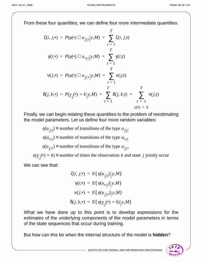
INSTITUTE FOR SIGNAL AND INFORMATION PROCESSING
MAY 15-17, 1996 TEXAS INSTRUMENTS PAGE 98 OF 147
From these four quantities, we can define four more intermediate quantities:
Finally, we can begin relating these quantities to the problem of reestimatingthe model parameters. Let us define four more random variables:
We can see that:
What we have done up to this point is to develop expressions for theestimates of the underlying components of the model parameters in termsof the state sequences that occur during training.
But how can this be when the internal structure of the model is hidden ?
ζ i j, •;( ) P u •( ) uj i∈ y M,( ) ζ i j, t;( )
t 1=
T
∑= =
γ i •;( ) P u •( ) u• i∈ y M,( ) γ i t;( )
t 1=
T
∑= =
ν j •;( ) P u •( ) uj •∈ y M,( ) ν j t;( )
t 1=
T
∑= =
δ j k •;,( ) P yj
•( ) k= y M,( ) δ j k t;,( )
t 1=
T
∑ ν j t;( )
t 1=
y t( ) k=
T
∑= = =
n uj i( ) number of transitions of the typeuj i≡
n u• i( ) number of transitions of the typeu• i≡
n uj •( ) number of transitions of the typeuj •≡
n yj
•( ) k=( ) number of times the observationk and statej jointly occur≡
ζ i j, •;( ) E n uj i( ) y M, =
γ i •;( ) E n u• i( ) y M, =
ν j •;( ) E n uj •( ) y M, =
δ j k •;,( ) E n yj
•( ) k=( ) y M, =

INSTITUTE FOR SIGNAL AND INFORMATION PROCESSING
MAY 15-17, 1996 TEXAS INSTRUMENTS PAGE 99 OF 147
Following this line of reasoning, an estimate of the transition probability is:
Similarly,
Finally,
This process is often called reestimation by recognition, because we needto recognize the input with the previous models in order that we cancompute the new model parameters from the set of state sequences used torecognize the data (hence, the need to iterate).
But will it converge? Baum and his colleagues showed that the new modelguarantees that:
a j i( )E n uj i( ) y M,
E n u• i( ) y M, --------------------------------------- ζ i j, •;( )
γ i •;( )------------------= =
α y1t
i,( )a j i( )b y t 1+( ) j( )β yt 2+T
j( )
t 1=
T 1–
∑
α y1t
i,( )β yt 1+T
i( )
t 1=
T 1–
∑-------------------------------------------------------------------------------------------------=
b k j( )
E n n yj
•( ) k=( ) y M,( ) y M,
E n uj •( ) y M, ----------------------------------------------------------------------- ζ i j, •;( )
γ i •;( )------------------= =
α y1t
j,( )β ytT
j( )
t 1=y t( ) k=
T
∑
α y1t
j,( )β yt 1+T
j( )
t 1=
T
∑------------------------------------------------------=
P x 1( ) i=( )α y1
1i,( )β y2
Ti( )
P y M( )----------------------------------=
P y M( ) P y M( )≥
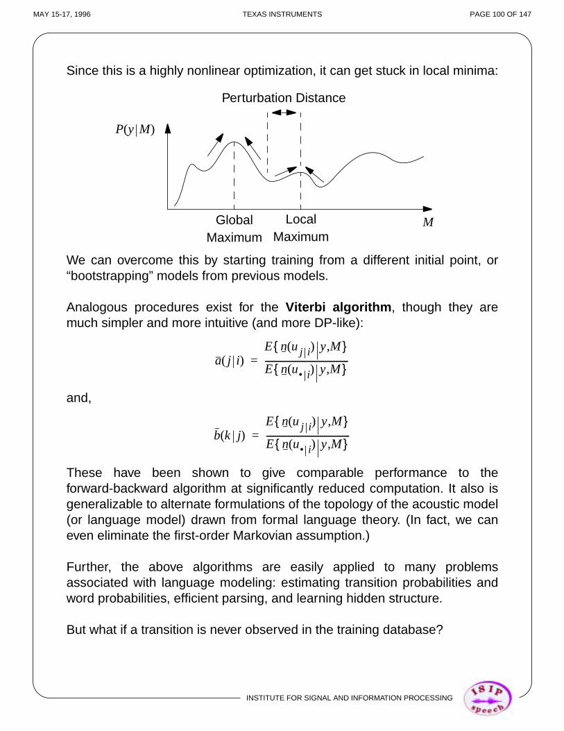
MAY 15-17, 1996 TEXAS INSTRUMENTS PAGE 100 OF 147
Since this is a highly nonlinear optimization, it can get stuck in local minima:
P y M( )
MGlobalMaximum
LocalMaximum
Perturbation Distance
We can overcome this by starting training from a different initial point, or“bootstrapping” models from previous models.
Analogous procedures exist for the Viterbi algorithm , though they aremuch simpler and more intuitive (and more DP-like):
and,
These have been shown to give comparable performance to theforward-backward algorithm at significantly reduced computation. It also isgeneralizable to alternate formulations of the topology of the acoustic model(or language model) drawn from formal language theory. (In fact, we caneven eliminate the first-order Markovian assumption.)
Further, the above algorithms are easily applied to many problemsassociated with language modeling: estimating transition probabilities andword probabilities, efficient parsing, and learning hidden structure.
But what if a transition is never observed in the training database?
a j i( )E n uj i( ) y M,
E n u• i( ) y M, ---------------------------------------=
b k j( )E n uj i( ) y M,
E n u• i( ) y M, ---------------------------------------=
INSTITUTE FOR SIGNAL AND INFORMATION PROCESSING

MAY 15-17, 1996 TEXAS INSTRUMENTS PAGE 101 OF 147
Continuous Density HMMs
The discrete HMM incorporates a discrete probability density function,captured in the matrix , to describe the probability of outputting a symbol:B
output distribution for state kb k j( )
k1 2 3 4 5 6 • • •
Signal measurements, or feature vectors, are continuous-valuedN-dimensional vectors. In order to use our discrete HMM technology, wemust vector quantize (VQ) this data — reduce the continuous-valuedvectors to discrete values chosen from a set of M codebook vectors. Initially,most HMMs were based on VQ front-ends. However, recently, thecontinuous density model has become widely accepted.Let us assume a parametric model of the observation pdf:The likelihood of generating observation in state is defined as:
Note that taking the negative logarithm of will produce a log-likelihood,or a Mahalanobis-like distance. But what form should we choose for ?Let’s assume a Gaussian model, of course:
Note that this amounts to assigning a mean and covariance matrix to eachstate — a significant increase in complexity. However, shortcuts such asvariance-weighting can help reduce complexity.
Also, note that the log of the output probability at each state becomesprecisely the Mahalanobis distance (principal components) we studied atthe beginning of the course.
M S π 1( ) A f y x ξ i( ) 1 i S≤ ≤,
, , ,
=
y t( ) j
b y t( ) j( ) f y x y t( ) j( )≡
b( )
f ( )
f y x y i( )1
2π Ci
------------------- 12---– y µi–( )T
Ci1–
y µi–( )
exp=
INSTITUTE FOR SIGNAL AND INFORMATION PROCESSING

MAY 15-17, 1996 TEXAS INSTRUMENTS PAGE 102 OF 147
Mixture Distributions
Of course, the output distribution need not be Gaussian, or can bemultimodal to reflect the fact that several contexts are being encoded into asingle state (male/female, allophonic variations of a phoneme, etc.). Muchlike a VQ approach can model any discrete distribution, we can use aweighted linear combination of Gaussians, or a mixture distribution, toachieve a more complex statistical model.
b y j( ) three mixturescomposite (offset)
y
u1 u2 u3
Mathematically, this is expressed as:
In order for this to be a valid pdf, the mixture coefficients must benonnegative and satisfy the constraint:
Note that mixture distributions add significant complexity to the system: mmeans and covariances at each state.
Analogous reestimation formulae can be derived by defining theintermediate quantity:
f y x y i( ) cimℵ y µim Cim,;( )
m 1=
M
∑=
cimm 1=
M
∑ 1= , 1 i S≤ ≤
ν i t l,;( ) P x t( ) i= y t( )produced in accordance with mixturel( )≡
α y1t
i,( )β yt 1+T
i( )
α y1t
j,( )β yt 1+T
j( )
j 1=
S
∑-------------------------------------------------------
cil ℵ ytlt µil Cil,;( )
cimℵ ytt µim Cim,;( )
m 1=
M
∑----------------------------------------------------------×=
INSTITUTE FOR SIGNAL AND INFORMATION PROCESSING

INSTITUTE FOR SIGNAL AND INFORMATION PROCESSING
MAY 15-17, 1996 TEXAS INSTRUMENTS PAGE 103 OF 147
The mixture coefficients can now be reestimated using:
the mean vectors can be reestimated as:
the covariance matrices can be reestimated as:
and the transition probabilities, and initial probabilities are reestimated asusual.
The Viterbi procedure once again has a simpler interpretation:
and
The mixture coefficient is reestimated as the number of vectors associatedwith a given mixture at a given state:
cilν i • l,;( )
ν i • m,;( )
m 1=
M
∑--------------------------------=
µil
ν i t l,;( ) y t( )
t 1=
T
∑ν i • l,;( )
------------------------------------=
Cil
ν i t l,;( ) y t( ) µil–[ ] y t( ) µil–[ ]T
t 1=
T
∑ν i • l,;( )
------------------------------------------------------------------------------------=
µil1
Nil------- y t( )
t 1=y t( ) il∼
T
∑=
Cil1
Nil------- y t( ) µil–[ ] y t( ) µil–[ ]T
t 1=y t( ) il∼
T
∑=
cil
Nil
Ni-------=

INSTITUTE FOR SIGNAL AND INFORMATION PROCESSING
MAY 15-17, 1996 TEXAS INSTRUMENTS PAGE 104 OF 147
Session VII:
Acoustic Modeling and Training
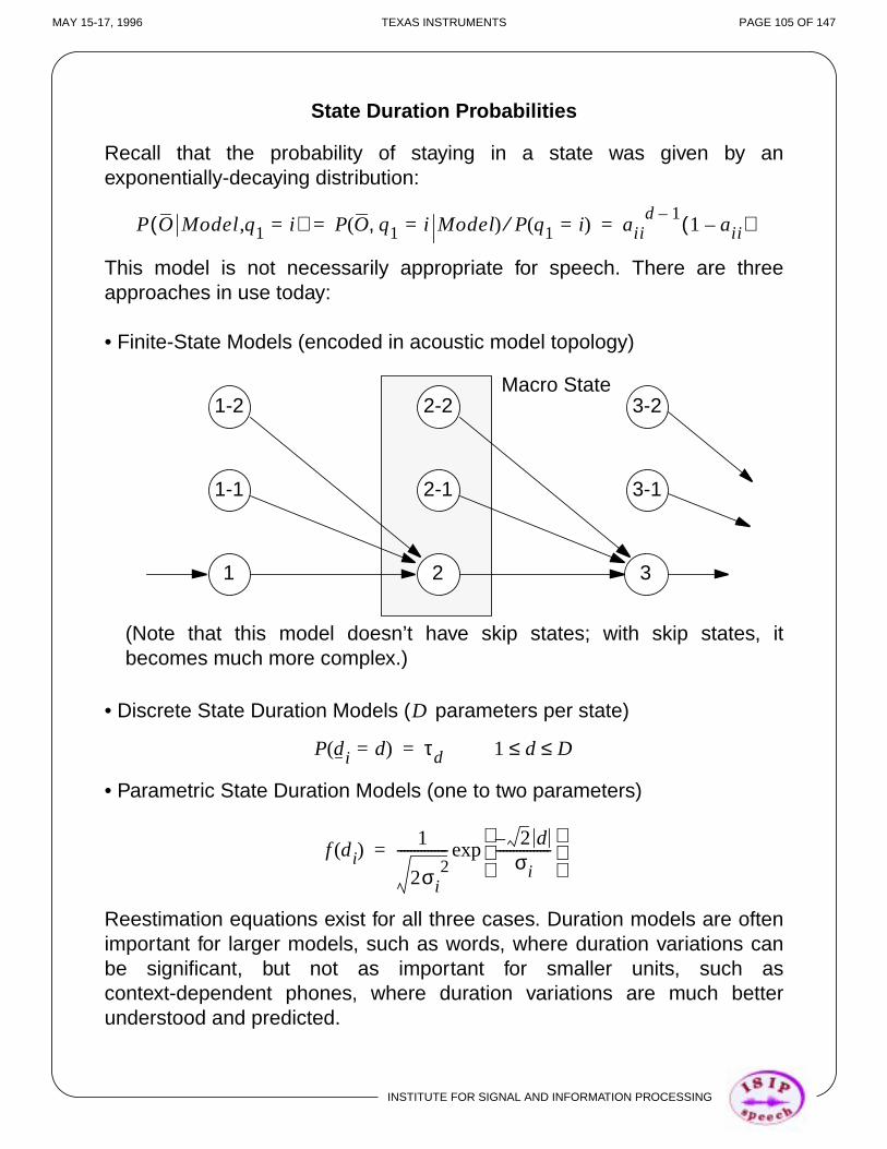
MAY 15-17, 1996 TEXAS INSTRUMENTS PAGE 105 OF 147
State Duration Probabilities
Recall that the probability of staying in a state was given by anexponentially-decaying distribution:
This model is not necessarily appropriate for speech. There are threeapproaches in use today:
• Finite-State Models (encoded in acoustic model topology)
P O Model q1 i=,( ) P O q1 i=, Model( ) P q1 i=( )⁄ aiid 1–
1 aii–( )= =
1 2 3
1-1
1-2
2-1
2-2
3-1
3-2Macro State
(Note that this model doesn’t have skip states; with skip states, itbecomes much more complex.)
• Discrete State Duration Models ( parameters per state)
• Parametric State Duration Models (one to two parameters)
Reestimation equations exist for all three cases. Duration models are oftenimportant for larger models, such as words, where duration variations canbe significant, but not as important for smaller units, such ascontext-dependent phones, where duration variations are much betterunderstood and predicted.
D
P di d=( ) τd= 1 d D≤ ≤
f di( )1
2σi2
--------------- 2 d–σi
----------------
exp=
INSTITUTE FOR SIGNAL AND INFORMATION PROCESSING

INSTITUTE FOR SIGNAL AND INFORMATION PROCESSING
MAY 15-17, 1996 TEXAS INSTRUMENTS PAGE 106 OF 147
Scaling in HMMs
As difficult as it may seem to believe, standard HMM calculations exceedthe precision of 32-bit floating point numbers for the simplest of models. Thelarge numbers of multiplications of numbers less than one leads tounderflow. Hence, we must incorporate some form of scaling.
It is possible to scale the forward-backward calculation (see Section 12.2.5)by normalizing the calculations by:
at each time-step (time-synchronous normalization).
However, a simpler and more effective way to scale is to deal with logprobabilities, which work out nicely in the case of continuous distributions.Even so, we need to somehow prevent the best path score from growingwith time (increasingly negative in the case of log probs). Fortunately, ateach time step, we can normalize all candidate best-path scores, andproceed with the dynamic programming search. More on this later...
Similarly, it is often desirable to trade-off the important of transitionprobabilities and observation probabilities. Hence, the log-likelihood of anoutput symbol being observed at a state can be written as:
or, in the log prob space:
This result emphasizes the similarities between HMMs and DTW. Theweights, and can be used to control the importance of the “languagemodel.”
c t( ) 1
α y1t
i,( )
i 1=
S
∑---------------------------=
P y1t
x t( ) i=( ), y M,( ) P x t 1–( ) j= y M,( ) aij( )αbi y t( )( )
β+=
P y1t …,( )
log P x t 1–( ) j=( )… log α aij( )log+ β Dy µ,log+=
α β

MAY 15-17, 1996 TEXAS INSTRUMENTS PAGE 107 OF 147
STr
An Overview of the Training Schedule
Seed Model Construction
Build Grammar
Recognize
Backtrace/Update
Replace Parameters
Next Utterance
Next Iteration
Hand-Excised Data
Last Utterance?
Convergence?
upervisedaining
Note that a priori segmentation of the utterance is not required, and that therecognizer is forced to recognize the utterance during training (via the buildgrammar operation). This forces the recognizer to learn contextualvariations, provided the seed model construction is done “properly.”
What about speaker independence?Speaker dependence?Speaker adaptation?Channel adaptation?
INSTITUTE FOR SIGNAL AND INFORMATION PROCESSING
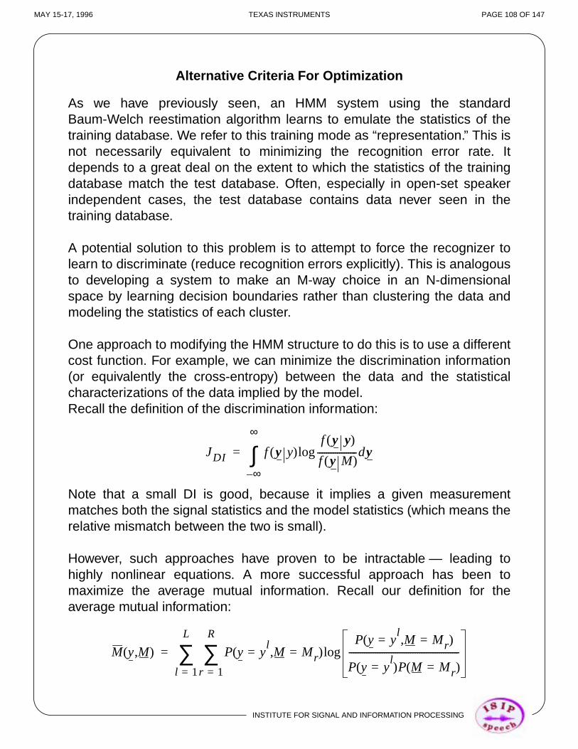
INSTITUTE FOR SIGNAL AND INFORMATION PROCESSING
MAY 15-17, 1996 TEXAS INSTRUMENTS PAGE 108 OF 147
Alternative Criteria For Optimization
As we have previously seen, an HMM system using the standardBaum-Welch reestimation algorithm learns to emulate the statistics of thetraining database. We refer to this training mode as “representation.” This isnot necessarily equivalent to minimizing the recognition error rate. Itdepends to a great deal on the extent to which the statistics of the trainingdatabase match the test database. Often, especially in open-set speakerindependent cases, the test database contains data never seen in thetraining database.
A potential solution to this problem is to attempt to force the recognizer tolearn to discriminate (reduce recognition errors explicitly). This is analogousto developing a system to make an M-way choice in an N-dimensionalspace by learning decision boundaries rather than clustering the data andmodeling the statistics of each cluster.
One approach to modifying the HMM structure to do this is to use a differentcost function. For example, we can minimize the discrimination information(or equivalently the cross-entropy) between the data and the statisticalcharacterizations of the data implied by the model.Recall the definition of the discrimination information:
Note that a small DI is good, because it implies a given measurementmatches both the signal statistics and the model statistics (which means therelative mismatch between the two is small).
However, such approaches have proven to be intractable — leading tohighly nonlinear equations. A more successful approach has been tomaximize the average mutual information. Recall our definition for theaverage mutual information:
JDI f y y( )f y y( )
f y M( )------------------log yd
∞–
∞
∫=
M y M,( ) P y yl
= M Mr=,( )P y y
l= M Mr=,( )
P y yl
=( )P M Mr=( )--------------------------------------------------log
r 1=
R
∑l 1=
L
∑=

INSTITUTE FOR SIGNAL AND INFORMATION PROCESSING
MAY 15-17, 1996 TEXAS INSTRUMENTS PAGE 109 OF 147
This can be written as:
Note that the last term constitutes a rewrite of .
If we assume there is exactly one training string (which is the error we wantto correct), and it is to be used to train , then, if we assume
, we can approximate by:
The first term in the summation corresponds to the probability of correctrecognition, which we want to maximize. The second term corresponds tothe probability of incorrect recognition, which we want to minimize.
This method has a rather simple interpretation for discrete HMMs:
M y M,( ) P y yl
= M Mr=,( ) ×r 1=
R
∑l 1=
L
∑=
P y yl
= M Mr=,( )[ ]log P y yl
=( )[ ]log–
P y yl
= M Mr=,( ) ×r 1=
R
∑l 1=
L
∑=
[ P y yl
= M Mr=,( )log –
P y yl
= M Mm=( )P M Mm=( ) ]
m 1=
R
∑log
P y yl
=( )
Ml
P y yl
= M Mr=( ) δ l r–( )≈ M y M,( )
M y M,( ) P y yl
= M Ml=,( )
l 1=
L
∑ P y yl
= M Mm=( )P M Mm=( )
m 1=
R
∑log–≈
21
53 4
76 8
Increment Counts Along Best Path
Decrement Counts Along Competing Incorrect Paths

INSTITUTE FOR SIGNAL AND INFORMATION PROCESSING
MAY 15-17, 1996 TEXAS INSTRUMENTS PAGE 110 OF 147
An Overview of the Corrective Training Schedule
Seed Model Construction
Build Grammar
Backtrace/Update
Replace Parameters
Next Utterance
Next Iteration
Hand-Excised Data
Last Utterance?
Convergence?
SupervisedTraining
Recognize
Recognize (Open)
Recognition Error
Backtrace/Update
Replace Parameters
Next UtteranceLast Utterance?
Convergence?
CorrectiveTraining

INSTITUTE FOR SIGNAL AND INFORMATION PROCESSING
MAY 15-17, 1996 TEXAS INSTRUMENTS PAGE 111 OF 147
Unfortunately, this method is not readily extensible to continuous speech,and has proved inconclusive in providing measurable reductions in errorrate. However, discriminative training algorithms continues to be animportant are of research in HMMs.
Later, when we study neural networks, we will observe that some of theneural network approaches are ideally suited towards implementation ofdiscriminative training.
Distance Measures for HMMs
Recall the KMEANS clustering algorithm:
Initialization: Choose K centroids
Recursion: 1. Assign all vectors to their nearest neighbor.
2. Recompute the centroids as the average of all vectorsassigned to the same centroid.
3. Check the overall distortion. Return to step 1 if somedistortion criterion is not met.
Clustering of HMM models is often important in reducing the number ofcontext-dependent phone models (which can often approach 10,000 forEnglish) to a manageable number (typically a few thousand models areused). We can use standard clustering algorithms, but we need some way ofcomputing the distance between two models.
A useful distance measure can be defined as:
where is a sequence generated by of length . Note that this
distance metric is not symmetric:
D M1 M2,( )1
T2------ P y
2M1( )log P y
2M2( )log–[ ]≡
y2
M2 T2
D M1 M2,( ) D M2 M1,( )≠

INSTITUTE FOR SIGNAL AND INFORMATION PROCESSING
MAY 15-17, 1996 TEXAS INSTRUMENTS PAGE 112 OF 147
A symmetric version of this is:
The sequence is often taken to be the sequence of mean vectorsassociated with each state (typically for continuous distributions).
Often, phonological knowledge is used to cluster models. Models sharingsimilar phonetic contexts are merged to reduce the complexity of the modelinventory. Interestingly enough, this can often be performed by inserting anadditional network into the system that maps context-dependent phonemodels to a pool of states.
D' M1 M2,( )D M1 M2,( ) D M2 M1,( )+
2-----------------------------------------------------------=
y2

INSTITUTE FOR SIGNAL AND INFORMATION PROCESSING
MAY 15-17, 1996 TEXAS INSTRUMENTS PAGE 113 OF 147
The DTW Analogy
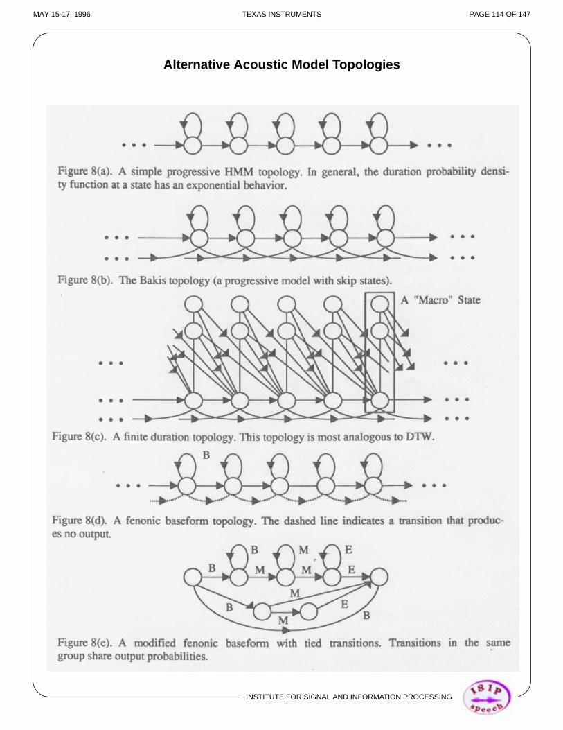
INSTITUTE FOR SIGNAL AND INFORMATION PROCESSING
MAY 15-17, 1996 TEXAS INSTRUMENTS PAGE 114 OF 147
Alternative Acoustic Model Topologies

INSTITUTE FOR SIGNAL AND INFORMATION PROCESSING
MAY 15-17, 1996 TEXAS INSTRUMENTS PAGE 115 OF 147
Managing Model Complexity
Continuous DensityMixture Distributions
Discrete DensityVector Quantization
Semi-Continuous HMMs
Tied States
Clustered States
Tied Mixtures
Increasing Memory
Increasing Number of Free Parameters
Increasing Performance?
Increasing CPU
Increasing Storage
• Numerous techniques to robustly estimate model parameters; among themost popular is deleted interpolation:
A εt At 1 εt–( )Au+=
B εtBt 1 εt–( )Bu+=

INSTITUTE FOR SIGNAL AND INFORMATION PROCESSING
MAY 15-17, 1996 TEXAS INSTRUMENTS PAGE 116 OF 147
Seed Model Construction: Duration Distributions

INSTITUTE FOR SIGNAL AND INFORMATION PROCESSING
MAY 15-17, 1996 TEXAS INSTRUMENTS PAGE 117 OF 147
Seed Model Construction: Number of States Proportional to Duration

INSTITUTE FOR SIGNAL AND INFORMATION PROCESSING
MAY 15-17, 1996 TEXAS INSTRUMENTS PAGE 118 OF 147
Duration in Context Clustering

INSTITUTE FOR SIGNAL AND INFORMATION PROCESSING
MAY 15-17, 1996 TEXAS INSTRUMENTS PAGE 119 OF 147
Examples of Word Models

INSTITUTE FOR SIGNAL AND INFORMATION PROCESSING
MAY 15-17, 1996 TEXAS INSTRUMENTS PAGE 120 OF 147
Session VIII:
Speech RecognitionUsing
Hidden Markov Models

INSTITUTE FOR SIGNAL AND INFORMATION PROCESSING
MAY 15-17, 1996 TEXAS INSTRUMENTS PAGE 121 OF 147
BASIC TECHNOLOGY:
A PATTERN RECOGNITION PARADIGM
BASED ON HIDDEN MARKOV MODELS
Search Algorithms:P Wti
Ot( )P Ot Wt
i( )P Wt
i( )
P Ot( )--------------------------------------=
Pattern Matching: Wti
P Ot Ot 1– … Wti, ,( ),[ ]
Signal Model:P Ot Wt 1– Wt Wt 1+, ,( )( )
Recognized Symbols:P S O( ) maxargT
P Wti
Ot Ot 1– …, ,( )( )i
∏=
Language Model:P Wti
( )
Prediction

INSTITUTE FOR SIGNAL AND INFORMATION PROCESSING
MAY 15-17, 1996 TEXAS INSTRUMENTS PAGE 122 OF 147
Nonspeech
High Performance Isolated Word RecognitionUsing A Continuous Speech Recognizer
1 2
Isolated Word Recognition:
Nonspeech
WordS S
Nonspeech:typically an acoustic model of one frame in duration thatmodels the background noise.
Word: any word from the set of possible words that can be spoken
• The key point here is that, with such a system, the recognizer finds theoptimal start/stop times of the utterance with respect to the acousticmodel inventory (a hypothesis-directed search)
1
Simple Continuous Speech Recognition (“No Grammar”):
Nonspeech/Word
Nonspeech Nonspeech
SNonspeech
SNonspeech
• system recognizes arbitrarily long sequences of words or nonspeech events

INSTITUTE FOR SIGNAL AND INFORMATION PROCESSING
MAY 15-17, 1996 TEXAS INSTRUMENTS PAGE 123 OF 147
The Great Debate: “Bottom-Up” or “Top-Down”
S
NP V CONJ PRON V PP
ART N
THE CHILD CRIED AS SHE LEFT IN THE RED PLANE
PREP NP
ART ADJ N
D x C Y l d k r Y d x S S i l E f t I n D x r E d p l e n
Parsing refers to the problem of determining if a given sequence could havebeen generated from a given state machine.
This computation, as we shall see, typically requires an elaborate search of allpossible combinations of symbols output from the state machine.
This computation can be efficiently performed in a “bottom-up” fashion if theprobabilities of the input symbols are extremely accurate, and only a fewsymbols are possible at each point at the lower levels of the tree.
If the input symbols are ambiguous, “top-down” parsing is typically preferred.

INSTITUTE FOR SIGNAL AND INFORMATION PROCESSING
MAY 15-17, 1996 TEXAS INSTRUMENTS PAGE 124 OF 147
Network Searching and Beam Search
Premise: Suboptimal solutions are useful; global optimums are hard to find.
2
1
3
4
••
••
••
6
5
7
8
••
••
••
j
The network search considers several competing constraints:
• The longer the hypothesis, the lower the probability
• The overall best hypothesis will not necessarily be the best initialhypothesis
• We want to limit the evaluation of the same substring by differenthypotheses (difficult in practice)
• We would like to maintain as few active hypotheses as possible
• All states in the network will not be active at all times
6
5
7
8
••
••
••
Best Path

INSTITUTE FOR SIGNAL AND INFORMATION PROCESSING
MAY 15-17, 1996 TEXAS INSTRUMENTS PAGE 125 OF 147
Popular Search Algorithms
• Time Synchronous (Viterbi, DP)
• State Synchronous (Baum-Welch)
• Stack Decoding (N-Best, Best-First, A*)
• Hybrid Schemes
— Forward-Backward
— Multipass
— Fast Matching

MAY 15-17, 1996 TEXAS INSTRUMENTS PAGE 126 OF 147
zer
oh
0.1
zeo
Generalization of the HMM
Consider the following state diagram showing a simple language modelinvolving constrained digit sequences:
one (1.0)
S
A
o (0.3)
(0.7) 0.5
one (0.3)
five (0.5)
0.5
one (0.8)six (0.2)
ro (0.3)h (0.7)
0.9
three (1.0) four (1.0)two (1.0)
B C D Etwo (1.0) three (1.0) four (1.0)
0.9 0.9 0.9
0.1 0.1 0.1 0.1
eight (1.0)
seven (0.5)four (0.5)
six (1.0)
G H
I
Jfive (0.8)zero (0.1)
F
oh (0.1)
eight (1.0)
nine (1.0)
five (1.0)
six (1.0)
0.9
0.9
0.4
0.4
1.0
1.0
0.1 0.1 0.2
seven (1.0)
0.9
nine (1.0)Note the similarities to our acoustic models.
What is the probability of the sequence “zero one two three four five zero sixsix seven seven eight eight” ?
How would you find the average length of a digit sequence generated fromthis language model?
INSTITUTE FOR SIGNAL AND INFORMATION PROCESSING

INSTITUTE FOR SIGNAL AND INFORMATION PROCESSING
MAY 15-17, 1996 TEXAS INSTRUMENTS PAGE 127 OF 147
In the terminology associated with formal language theory, this HMM isknown as a finite state automaton.
The word stochastic can also be applied because the transitions and outputsymbols are governed by probability distributions.
Further, since there are multiple transitions and observations generated atany point in time (hence, ambiguous output), this particular graph isclassified as a nondeterministic automaton.
In the future, we will refer to this system as a stochastic finite stateautomaton (FSA or SFSA) when it is used to more linguistic information.
We can also express this system as a regular grammar:
S zero, Ap1
S oh, Ap2
S one, Ap3
S five, Ap4
A zero, Ap5
A oh, Ap6
A one, Bp7
A six, Bp8
B one, Bp9
B two, Cp10
C two, Cp11
C three, Dp12
D three, Dp13
D four, Ep14
E four, Ep15
E five, Fp16
F zero, Fp17
F oh, Fp18
F five, Fp19
F six, Gp20
G six, Gp21
G seven, Hp22
H seven, Hp23
H four, Hp24
H eight, Ip25
H nine, Jp26
I eight, Ip’27
I eight.p”27
I nine, Jp’28
I nine.p”28

INSTITUTE FOR SIGNAL AND INFORMATION PROCESSING
MAY 15-17, 1996 TEXAS INSTRUMENTS PAGE 128 OF 147
Note that rule probabilities are not quite the same as transition probabilities,since they need to combine transition probabilities and output probabilities.For example, consider p7:
In general,
Note that we must adjust probabilities at the terminal systems when thegrammar is nondeterministic:
to allow generation of a final terminal.
Hence, our transition from HMMs to stochastic formal languages is clearand well-understood.
p7 0.9( ) 0.8( )=
P y yk= x xi=( ) aij b k( )j
∑=
pk p'k p''k+=

INSTITUTE FOR SIGNAL AND INFORMATION PROCESSING
MAY 15-17, 1996 TEXAS INSTRUMENTS PAGE 129 OF 147
The Artificial Neural Network (ANN)
Premise: complex computational operations can be implemented by
massive integration of individual components
Topology and interconnections are key: in many ANN systems,
spatial relationships between nodes have some physical relevance
Properties of large-scale systems: ANNs also reflect a growing body
of theory stating that large-scale systems built from a small unit neednot simply mirror properties of a smaller system (contrast fractalsand chaotic systems with digital filters)
Why Artificial Neural Networks?
Important physical observations:
— The human central nervous system contains 1011 — 1014 nerve
cells, each of which interacts with 103 — 104 other neurons
— Inputs may be excitatory (promote firing) or inhibitory
∫ S •( )
node: nk
y’1
y’2
y’3
Θk
yk
The Artificial Neuron — Nonlinear
scalar outputvector input
yk S wki y'in 1=
N
∑ θk–( )≡
bk yk( )
node: nk
aik
aik
alkakq
akr
aks
The HMM State — Linear
α y1t 1+
j,( ) α y1t
i,( )a j i( )b y t 1+( ) j( )=

INSTITUTE FOR SIGNAL AND INFORMATION PROCESSING
MAY 15-17, 1996 TEXAS INSTRUMENTS PAGE 130 OF 147
Typical Thresholding Functions — A Key Difference
The input to the thresholding function is a weighted sum of the inputs:
The output is typically defined by a nonlinear function:
uk wkT
y'≡
S(u)
u
S(u) S(u)
S(u)
1
1
u
uu
1
Linear Ramp
Step Sigmoid S u( ) 1 eu–
+( )1–
=
Sometimes a bias is introduced into the threshold function:
This can be represented as an extra input whose value is always -1:
yk S wkT
y' θk–( )≡ S uk θk–( )=
y'N 1+ 1–= wk N 1+, θk=

MAY 15-17, 1996 TEXAS INSTRUMENTS PAGE 131 OF 147
Radial Basis Functions
Another popular formulation involves the use of a Euclidean distance:
Note the parallel to a continuous distribution HMM.
This approach has a simple geometric interpretation:
yk S wik y'i–( )2
i 1=
N
∑ θk–( ) S wk y'–2
θk–( )= =
wk
Θk
y’1
y’2S(u)
u
1
Another popular variant of this design is to use a Gaussian nonlinearity:
What types of problems are such networks useful for?
• pattern classification (N—way choice; vector quantization)
• associative memory (generate an output from a noisy input;character recognition)
• feature extraction (similarity transformations; dimensionalityreduction)
We will focus on multilayer perceptrons in our studies. These have beenshown to be quite useful for a wide range of problems.
S u( ) eu2–
=
INSTITUTE FOR SIGNAL AND INFORMATION PROCESSING

MAY 15-17, 1996 TEXAS INSTRUMENTS PAGE 132 OF 147
Multilayer Perceptrons (MLP)
This architecture has the following characteristics:
• Network segregated into layers: Ni cells per layer, L layers
• feedforward, or nonrecurrent, network (no feedback from the output of anode to the input of a node)
x0 x1 ... xN
y0 y1 ... yN
Input Layer
Hidden Layer
Output Layer
An alternate formulation of such a net is known as the learning vectorquantizer (LVQ) — to be discussed later.
The MLP network, not surprisingly, uses a supervised learning algorithm.The network is presented the input and the corresponding output, and mustlearn the optimal weights of the coefficients to minimize the differencebetween these two.
The LVQ network uses unsupervised learning — the network adjusts itselfautomatically to the input data, thereby clustering the data (learning theboundaries representing a segregation of the data). LVQ is popular becauseit supports discriminative training.
INSTITUTE FOR SIGNAL AND INFORMATION PROCESSING

MAY 15-17, 1996 TEXAS INSTRUMENTS PAGE 133 OF 147
Why Artificial Neural Networks?
• An ability to separate classes that are not linearly separable:
A
B
A
B
Linearly Separable
DecisionBoundary
Meshed Classes
A three-layer perceptron is required to determine arbitrarily-shaped decisionregions.
• Nonlinear statistical models
The ANN is capable of modeling arbitrarily complex probabilitydistributions, much like the difference between VQ and continuousdistributions in HMM.
• Context-sensitive statistics
Again, the ANN can learn complex statistical dependencies providedthere are enough degrees of freedom in the system.
Why not Artificial Neural Networks? (The Price We Pay...)
• Difficult to deal with patterns of unequal length
• Temporal relationships not explicitly modeled
And, of course, both of these are extremely important to the speechrecognition problem.
INSTITUTE FOR SIGNAL AND INFORMATION PROCESSING

INSTITUTE FOR SIGNAL AND INFORMATION PROCESSING
MAY 15-17, 1996 TEXAS INSTRUMENTS PAGE 134 OF 147
Session IX:
Language Modeling

INSTITUTE FOR SIGNAL AND INFORMATION PROCESSING
MAY 15-17, 1996 TEXAS INSTRUMENTS PAGE 135 OF 147
Perplexity
How do we evaluate the difficulty of a recognition task?
• Instantaneous/local properties that influence peak resource requirements:maximum number of branches at a node; acoustic confusability
• Global properties that influence average difficulty: perplexity
If there are possible words output from a random source, and the source isnot statistically independent (as words in a language tend to be), the entropyassociated with this source is defined as:
For an ergodic source, we can compute temporal averages:
Of course, these probabilities must be estimated from training data (or test data).
Perplexity, a common measure used in speech recognition, is simply:
and represents the average branching factor of the language.
Perplexities range from 11 for digit recognition to several hundred for LVCSR. Fora language in which all words are equally likely for all time,
W
H w( )1N---- E P w1
Nw1
N=( )log
–
w1N
∑N ∞→lim–=
1N---- P w1
Nw1
N=( ) P w1
Nw1
N=( )log
w1N
∑N ∞→lim–=
H w( )1N---- P w1
Nw1
N=( )log
N ∞→lim–=
Q w( ) 2H w( )
=
Q w( ) W=

INSTITUTE FOR SIGNAL AND INFORMATION PROCESSING
MAY 15-17, 1996 TEXAS INSTRUMENTS PAGE 136 OF 147
Types of Language Models
Common Language Models:
• No Grammar (Digits)
• Sentence pattern grammars (Resource Management)
• Word Pair/Bigram (RM, Wall Street Journal)
• Word Class (WSJ, etc.)
• Trigram (WSJ, etc.)
• Back-Off Models (Merging Bigrams and Trigrams)
• Long Range N-Grams and Co-Occurrences (SWITCHBOARD)
• Triggers and Cache Models (WSJ)
• Link Grammars (SWITCHBOARD)
How do we deal with Out-Of-Vocabulary words?
• Garbage Models
• Monophone and Biphone Grammars with optional Dictionary Lookup
• Filler Models
Can we adapt the language model?

INSTITUTE FOR SIGNAL AND INFORMATION PROCESSING
MAY 15-17, 1996 TEXAS INSTRUMENTS PAGE 137 OF 147
Other Formal Languages
• Unrestricted Grammars
• Context Sensitive (N-Grams, Unification)
• Context Free (LR)
• Regular (or Finite State)
• Issues
— stochastic parsing
— memory, pruning, and complexity
ω1Aω2 ω1βω2→
A β→
A aB→A b→

INSTITUTE FOR SIGNAL AND INFORMATION PROCESSING
MAY 15-17, 1996 TEXAS INSTRUMENTS PAGE 138 OF 147
n i: z
NP[case:obj]
def:+ form: accnum: pltype: bodypart
The doctor examined the patient’s knees.Orthographic :
d A k t exrdh ex I g z ae m I n d dhex pH e-I sh I nt s
/# dh i # d A k t exr # I g z ae m ex n + d # dh i # p e sh ex n t + z # n i + z #/
Phonetic:
Phonemic:
VP
∃(X) & ∃(Y) & ∃(Z) & doctor(X) & patient(Y) & knees(Z) & part-of(Y,Z) & examined(X,Z)Logical:
S
NP[case:subj]
NP
NNDet
tense: pastarg1: subj[type:caregiver]
arg2: obj[type:bodypart]
V
form: gennum: singtype: patient
N
form: nomnum: singtype: caregiver
def:+
Det
Lexical:
Syntactic:
n i: zd A k t exr
0 1 20.5 1.5
5 kHz
0 kHz
4 kHz
3 kHz
2 kHz
1 kHz
Time (secs)
dh ex I g z ae m I n d dhex pH e-I sh I nt sPhonetic:
What can you do with all of this?

INSTITUTE FOR SIGNAL AND INFORMATION PROCESSING
MAY 15-17, 1996 TEXAS INSTRUMENTS PAGE 139 OF 147
Session IX:
State of the Art

INSTITUTE FOR SIGNAL AND INFORMATION PROCESSING
MAY 15-17, 1996 TEXAS INSTRUMENTS PAGE 140 OF 147
WHAT IS SPEECH UNDERSTANDING?
Speech Recognition: transcription of words
performance measured by word error rate
Speech understanding: acting on intentions
performance measured by the number of “queries” successfullyanswered (adds a natural language dimension to the problem)
DIMENSIONS OF THE PROBLEM
Performance is a function of the vocabulary
how many words are known to the system
how acoustically similar are the competing choices at each point
how many words are possible at each point in the dialog
Vocabulary size is a function of memory size
Usability is a function of the number of possiblecombinations of vocabulary words
restrictive syntax is good for performance and bad for usability
Hence, performance is a function of memory size

INSTITUTE FOR SIGNAL AND INFORMATION PROCESSING
MAY 15-17, 1996 TEXAS INSTRUMENTS PAGE 141 OF 147
Digit Recognition10 words
(perplexity = 10)
TODAY’S TECHNOLOGY
MIPS
10 10030
Memory
100K
1M
10M
100M NAB Newswire100K words
(perplexity =250)
Word Error Rate
Vocabulary Size (Words)
10 100 1K 10K
0.1%
1.0%
10.0%
100.0%
100K

INSTITUTE FOR SIGNAL AND INFORMATION PROCESSING
MAY 15-17, 1996 TEXAS INSTRUMENTS PAGE 142 OF 147
PROGRESS IN CSR PERFORMANCE
87 88 89.1 89.2 90 91 92a 92b 93 94
1
10
100
Word Error Rate (%)
Time
Resource Management (1000 Words) Wall Street Journal (5000 words) Wall Street Journal (20,000 words) NAB News (unlimited vocabulary)
Note: Machine performance is still at least two orders ofmagnitude lower than humans
(Data from George Doddington, ARPA HLT Program Manager, HLT’95)
5
50

INSTITUTE FOR SIGNAL AND INFORMATION PROCESSING
MAY 15-17, 1996 TEXAS INSTRUMENTS PAGE 143 OF 147
WHAT IS THE CONTEXT FOR SPEECHUNDERSTANDING RESEARCH IN THE 1990’s?
The Application Need
Interaction with on-line data (Internet)Automated information agents (“24-hour Help Desk”)Global multilingual interactions
The Technology Challenge
Create natural transparent interaction withcomputers (“2001,” “Star Trek”)
Bring computing to the masses (vanishing window)Intelligent presentation of information
(“hands/eyes busy applications”)
Application Areas
Command/Control (Telecom/Workstations)Database Query (Internet)Dictation (Workstations)Machine Translation (Workstations)Real-Time Interpretation (Telecom)

INSTITUTE FOR SIGNAL AND INFORMATION PROCESSING
MAY 15-17, 1996 TEXAS INSTRUMENTS PAGE 144 OF 147
THE TECHNICAL CHALLENGE
Barriers
Speech understanding is a vast empirical problem:
• Hierarchies of hidden representations (part-of-speech, nounphrases, units of meaning) produce immensely complex models
• Training of complex models requires huge and dynamic knowledgebases
Interconnected and interdependent levels ofrepresentation:
• Correct recognition and transcription of speech depends onunderstanding the meaning encoded in speech
• Correct understanding and interpretation of text depends on thedomain of discourse
Approach
Capitalize on exponential growth in computer powerand memory:
• Statistical modeling and automatic training• Shared resources and infrastructure
Application-focused technical tasks
• New metrics of performance based on user feedback andproductivity enhancement (human factors)
(G. Doddington, ARPA HLT Program Manager, “Spoken Language TechnologyDiscussion,” ARPA Human Language Technology Workshop, January 1995)

INSTITUTE FOR SIGNAL AND INFORMATION PROCESSING
MAY 15-17, 1996 TEXAS INSTRUMENTS PAGE 145 OF 147
Example No. 1: HTK (Cambridge University)
Signal Processing:
Sample Frequency = 16 kHzFrame Duration = 10 msWindow Duration = 25 ms (Hamming window)FFT-Based Spectrum AnalysisMel-Frequency Filter Bank (24)Log-DCT Cepstral Computation (Energy plus 12 coefficients)
Linear Regression Using A 5 Frame Window For andParameters
Acoustic Modeling:
Simple Left-To-Right Topology With Three Emitting States10 component Gaussian Mixtures at Each StateBaum-Welch ReestimationCross-Word Context-Dependent Phone ModelsState-Tying Using Phonetic Decision Trees (Common Broad
Phonetic Classes)+/- 2 Phones Used In Phonetic Decision Trees Including Word
Boundary
Language Modeling:
N-Gram Language Model (3, 4, and 5-Grams Have Been Reported)Discounting (De-Weight More Probable N-Grams)Back-Off Model Using BigramsSingle-Pass Time-Synchronous Tree Search
Notes:
Approx. 3 to 8 Million Free ParametersState-of-the-Art PerformanceRelatively Low ComplexityExcellent Real-Time Performance
∆ ∆2

INSTITUTE FOR SIGNAL AND INFORMATION PROCESSING
MAY 15-17, 1996 TEXAS INSTRUMENTS PAGE 146 OF 147
Example No. 2: Abbot Hybrid Connectionist HMM (Cambridge Univ.)
Signal Processing:
Sample Frequency = 16 kHzFrame Duration = 16 msWindow Duration = 32 msFFT-Based Spectrum AnalysisMel-Freq. Filter Bank (20) + 3 Voicing Features (replaced by PLP)Each Feature Normalized To Zero Mean and Unit Variance (Grand Covar.)
Acoustic Modeling:
Recurrent Neural NetworkSingle Layer Feed-Forward Network With Four Frame DelaySigmoidal NonlinearitiesA Single Network Computes All Posterior Phone ProbabilitiesViterbi-Like Back-Propagation-Through-Time TrainingParallel Combination of Backward-In-Time and Forward-In-Time NetworksContext-Dependent Probabilities Computed Using A Second LayerLinear Input Mapping For Speaker Adaptation (Similar to MLLR)
Language Modeling:
Single-Pass Stack Decoding AlgorithmN-Gram Language ModelPhone-Level and Word-Level PruningTree-Based LexiconNO Context-Dependent Cross-Word Models
Notes:
Approx. 80K Free ParametersPerformance Comparable To Best HMMsRelatively Low ComplexityExcellent Real-Time Performance

INSTITUTE FOR SIGNAL AND INFORMATION PROCESSING
MAY 15-17, 1996 TEXAS INSTRUMENTS PAGE 147 OF 147
Additional Resources
Web:
CMU: http://www.ri.cmu.edu/speech
comp.speech: ftp://svr-ftp.eng.cam.ac.uk/pub/pub/comp.speech/
UCSB: http://mambo.ucsc.edu/psl/speech.html
IEEE SP (Rice): http://spib.rice.edu/spib.html
Public Domain:
Oregon Graduate Institute
Cambridge Connectionist Group — AbbotDemo
... and many more ...
ISIP (about one year away)
Commercial:
Entropic Waves / HTK
Matlab (coming soon - also Entropic)