Fundamentals of Mathematical Statistics - Strojnícka...
85
Fundamentals of Mathematical Statistics Pavol ORANSK
Transcript of Fundamentals of Mathematical Statistics - Strojnícka...
Fundamentals of Mathematical Statistics
Pavol OR�ANSKÝ

2
Contents
1 Probability theory 91.1 Random event . . . . . . . . . . . . . . . . . . . . . . . . . . . . 9
1.1.1 Algebraic operations and programs with events . . . . . . 101.2 Classical de�nition of probability . . . . . . . . . . . . . . . . . . 121.3 Kolmogorov de�nition of probability . . . . . . . . . . . . . . . . 141.4 Probability of the uni�cation of random events . . . . . . . . . . 151.5 Probality of the opposite event . . . . . . . . . . . . . . . . . . . 171.6 Conditional probability . . . . . . . . . . . . . . . . . . . . . . . 181.7 Intersection probability of random phenomena . . . . . . . . . . 191.8 Full probability formula . . . . . . . . . . . . . . . . . . . . . . . 201.9 Bayesov vzorec . . . . . . . . . . . . . . . . . . . . . . . . . . . . 221.10 Bernoulliho vzorec . . . . . . . . . . . . . . . . . . . . . . . . . . 23
2 Random variable 252.1 Discrete probability distribution . . . . . . . . . . . . . . . . . . 252.2 Distribution function of random variable . . . . . . . . . . . . . . 272.3 Density distribution . . . . . . . . . . . . . . . . . . . . . . . . . 28
2.3.1 Basic features of the density distribution. . . . . . . . . . 292.4 Numerical characteristics of random variable . . . . . . . . . . . 31
2.4.1 Mean value . . . . . . . . . . . . . . . . . . . . . . . . . . 312.4.2 Variance (dispersion) and standard deviation . . . . . . . 33
3 Signi�cant continuous distribution of random variable 353.1 Normal distribution (Laplace-Gaussovo distribution) . . . . . . . 353.2 Standard normal distribution . . . . . . . . . . . . . . . . . . . . 36
3.2.1 The relationship between F (x) and �(x) . . . . . . . . . . 38
4 Descriptive statistics 41
5 Estimates of parameters 455.1 Point estimate . . . . . . . . . . . . . . . . . . . . . . . . . . . . 455.2 Interval estimation of parameters . . . . . . . . . . . . . . . . . . 49
5.2.1 100 � (1� �)% bilated con�dence interval for mean value � 495.2.2 100 � (1��)% bilateral con�dence interval for dispersion �2 53
3
4 CONTENTS
6 Testing statistical hypotheses 576.1 Parametric testing an single �le . . . . . . . . . . . . . . . . . . . 57
6.1.1 Testing parameter � if the set is small (n � 30) . . . . . . 596.1.2 Testing parameter � if the set is large (n > 30) . . . . . . 606.1.3 Testing parameter � . . . . . . . . . . . . . . . . . . . . . 61
6.2 Comparing two �les . . . . . . . . . . . . . . . . . . . . . . . . . 626.2.1 Testing equality of means of two fundamental �les, when
the �les are large (n > 30), and if �1, �2 are known . . . 626.2.2 Testing equality of means of two fundamental �les, when
the �les are small (n < 30), and if �1, �2 are known . . . 646.2.3 Testing equality of means of two fundamental �les, when
the �les are large (n > 30), and if �1, �2 are unknown . . 646.2.4 Testing equality of means of two fundamental �les, when
the �les are small (n < 30), and if �1, �2 are unknown . . 65
7 Correlation Analysis 697.1 Coe¢ cient covariance . . . . . . . . . . . . . . . . . . . . . . . . 697.2 Correlation coe¢ cient . . . . . . . . . . . . . . . . . . . . . . . . 707.3 Coe¢ cient of determination . . . . . . . . . . . . . . . . . . . . . 70
8 Paired linear regression 778.1 Regression line . . . . . . . . . . . . . . . . . . . . . . . . . . . . 778.2 Estimation of the parameters �0 and �1 . . . . . . . . . . . . . . 78
9 Attachments 81
Preface
This text was based on the inherent requirements of my students on the subjectof Statistics Faculty of Management, University of Pre�ov, an overview of acomprehensive publication of purely on statistics, contained in their basic course.Most existing text was either too large, and thus a deterrent to the reader, or,conversely, some publications contained only secondary curriculum. Demandson university students has recently changed considerably, therefore was also agap in the literature, which lacks books covering a kind of intermediate stage ofsecondary literature and literature explicitly university type, ie. kladúce booksto the reader requirements less stringent than in the past. This gap, I tried the"quick �x" patch overwrite my lectures from the course Statistics in acceptableform. I have text in addition to enriching addressed but not resolved by theexamples that I drew from its own resources respectively. I took them from thebook [1].1
This text does not replace any, in my opinion, excellent publications by otherauthors, of which I once again mention Chajdiaks [1]. But in some way tryingto bring modern students who are trying, let�s face it, as far as possible to savemathematics. It is strictly text reader for inexpensive, lightweight for deeperanalysis of issues.Finally, I would like to thank my colleague and good friend Dr., Ing. Ján RY-
BÁRIK, PhD., For their support and valuable advice of an experienced teacher,without whom this text would not arise. Also thank my students for comment.
Trenµcín, May 30, 2009 Pavol OR�ANSKÝ
1No results or arguments and examples used in them are not based on facts, and thereforethere is no real pre�guration them, which could be an eventual usurper can look up.
5

6 CONTENTS
Preface to the translation
This text was created, for the purpose of teaching foreign students, as a trans-lation of teaching material originally intended for teaching at the University ofPre�ov. Transfer and reducing the learning material we have created a textthat covers the issue of statistics needed to manage the course of numerical anddiscrete mathematics.Individual chapters present the minimum necessary for basic understanding
of statistical methods. The �rst chapter de�ned the very concept of probability,we deal with here its basic operations.In the second and third chapter describes some basic probability distribution.In the fourth chapter, the fundamentals of descriptive statistics, the neces-
sary basis for the data processed.The �fth chapter deals with the estimation of parameters.The sixth chapter is devoted to testing statistical hypotheses about the pa-
rameters set.Seventh and eighth chapter discusses the issue of linear dependency �les.
Trenµcín, January 2011 Pavol OR�ANSKÝ
7

8 CONTENTS
Chapter 1
Probability theory
Probability theory is a kind of basis for statistics. Is an integral part thereof. Fora deeper understanding of statistics is necessary to have knowledge of at leastthis chapter. Probability theory describes random events and probability of theoccurrence. Statistics speci�c model empirical events, and statistical methodsto describe these events have a fundamental right in probability theory.
1.1 Random event
De�nition 1 Random attempt (plot) is an attempt, the outcome is notclearly de�ned conditions, which were carried out. We have in mind attempts(even if the term �ts better story), whose outcome can not be determined inadvance.
For example: Coin toss or dice, the number of dead after a moderate earth-quake in China, the possibility of TB infection using trains Slovak railways, etc...
De�nition 2 Random event is true that the result of an accidental experi-ment. In other words, the outcome of the trial.
For example: "When throwing a coin falls symbol character", "The roll ofdice you get the number �ve", "When a moderate earthquake in China killed3624 people" or "While driving Slovak railways would be infected with TB everyone hundred �fty-nine billionth (wonderful word) the passengers�.Random events will be marked in capitals, eg.
event A ... "Hugo Chaves wins the presidential election in Venezuela."
In our view, are also interesting attempts, which will be studied event, theincreasing number of experiments show some stability. Which means that therelative frequency of the occurrence of accidental event A has an increasing
9
10 CHAPTER 1. PROBABILITY THEORY
number of trials tends to be constant. Where relative abundance is expressedas the ratio of "the occurrence of the event A" to "of all attempts.Therefore nothing other than
nAn� konst:, for n� 1;
nA indicates how many times there was a event A,n indicates the number of times an attempt was made.
We call this constant probability of accidental event A. (For the exampleabove, this probability is equal to the probability of the same event, as you saylater.)
For illustration, consider the dice with six sides and a random event A that"throwing the dice when you get the number �ve".If we started to throw the dice and the results we would be registered, after
a su¢ cient number of throws we would have noticed that the number of fallingnumbers �ve and the number of roll the dice in a ratio of about 1 to 6th Thisresult would probably not surprising, since almost everyone also expects that
the probability of "throwing the dice when you get the number �ve" is1
6=
0:166 67 $ 16:7%:
At this point we would like to alert readers to the increasingly paid attentionto the nomenclature of the probability theory, which as the years seem, alsotends to mislead, and therefore it is quite likely that the reader stops to focuson the issue, only because of uncertainties signs of inconsistency and opacity.
1.1.1 Algebraic operations and programs with events
Let A;B are random events.
I. Relation equality A = B
event A occurs if the event is part of B and B at the same event is partof the event A.
Eg.: event A ..." In throwing dice scored number six. "
event B ..." In throwing dice will fall even number divisible by three. "
II. Operation uni�cation A [B
Is a random event, which occurs if and only if there is a event A event or B,ie. occurs at least one of the events A or B.
Eg.: event A ..." In throwing dice scored number six. "
event B ..." In throwing dice scored number �ve. "
1.1. RANDOM EVENT 11
event A [B ..." In throwing dice scored number �ve or number six. "
III. Operation breakthrough A \B
Is a random event, which occurs if and only if there is a event A and B at thesame event occurs, ie. both events occur simultaneously.
Eg.: event A ..." In throwing dice scored number six. "
event B ..." In throwing dice scored number �ve. "
event A \ B ..." In throwing dice scored number �ve and number six atthe same time. "
IV. Opposite event �A
Contrary to the random event accidental event and occurs when the eventoccurs A.
Eg.: event A ..." In throwing dice scored number six. "
event �A ..." In throwing dice scored number six, ie. scored one of thenumbers one, two, three, four or �ve. "
V. Certain event
Certain event is a random event that always occurs.
Certain event ..." In throwing dice scored one of the numbers one, two, three,four, �ve or six. "
It could still possibly be that we fall on the edge of the cube but that it isimpossible.
Probably true is that A [ �A = :
VI. Impossible event ?
Impossible event is a random event that never occurs.
Eg.: event ..." when throwing dice, cube fall "(we think of anything moreimaginative)
Impossible event is the opposite event to the same event = ?.
Remark 1 If random events A \ B = ?, ie. if these two events never occursimultaneously, then these events are called disjoint (incompatible) randomevents.Eg.: Current tumble numbers two and three at once throwing dice.
Remark 2 Events can also compare, if A � B, then we call that event A eventis subevent B.
Remark 3 Eg.: event A ... "The roll of dice you get the number six."event B ... "In throwing dice will fall even number."
12 CHAPTER 1. PROBABILITY THEORY
1.2 Classical de�nition of probability
Probability should have similar properties as relative abundancenAn, since it is
modeled.For further understanding it is necessary to introduce some concepts that
we try to explain most empirically.
Event that can not be further broken down into detailed call elemental event,for example. when we throw dice event of falling even number decomposed intothree elementary events, namely: the event of falling number two, the event offalling numbers four and six event of falling numbers, which we can no longerspread, therefore it is elementary phenomena.
De�nition 3 The system of sets � called algebra, if:
1. 8A;B 2 �: A [B 2 �;
2. 8A;B 2 �: A \B 2 �;
3. 8A 2 � : A 2 �
4. 2 �;
5. ? 2 �:
De�nition 4 Real function P (A) de�ned on the algebra � subsets of will becalled if the following shall apply:
1. 8A 2 �) P (A) � 0;
2. 8A;B 2 �; : A \B = 0 (ie. disjoint) ) P (A [B) = P (A) + P (B);
3. P () = 1;
4. P (?) = 0.
De�nition 5 Assuming that the set of elementary events and is �nal, andwhile each elementary event is in addition to the same probability of getting aspecial case, so. classical de�nition of probability.
De�nition 6 Let be a �nite set, and let � be a algebra subset of the set ofelementary events .Then the probability P (A) of set A means the ratio
P (A) =jAjjj ;
where the symbol jAj means the number of elements set A and the symboljj means the number of elements set :
1.2. CLASSICAL DEFINITION OF PROBABILITY 13
Remark 4 Symbol jAj can be interpreted as a number of favorable results, ie.such results, in which event A occurs.Symbol jj represents the number of all possible outcomes when a random
experiment.
Remark 5 Trinity (; �; P ) will be called a probability space (classical).
Example 1 Throw dice. Calculate how likely that number will fall more than2
Solution: jAj = 4; since A = f3; 4; 5; 6g :jj = 6; since = f1; 2; 3; 4; 5; 6g :
P (A) =jAjjj =
4
6$ 0:67 = 67%:�
Example 2 Throw while playing with three dice. Vypoµcítajme what is likely tofall by three equal numbers?
Solution: jAj = 6:
jj = C 03(6) =�n+ k � 1
k
�=
�6 + 3� 1
3
�= 56:
P (A) =jAjjj =
6
56=3
280:107 = 10:7%:�
Example 3 V �katuli je 20 výrobkov, z toho 7 je nepodarkov. Náhodne vy-berieme 5 výrobkov. Vypoµcítame, aká je pravdepodobnos ,t, µze práve 2 medzivybranými výrobkami budú nepodarky?
Solution: jAj = C2(7) � C3(13) =�7
2
���13
3
�= 21 � 286 = 6006:
A - medzi vybranými budú dva nepodarky (tj. C2(7) =�7
2
�) a zvy�né tri
budú v poriadku (tj. C3(13) =�13
3
�).
jj = C5(20) =�20
5
�= 15 504:
- výber 5 z 20, priµcom na poradí nezáleµzí.
P (A) =jAjjj =
6006
15 504=1001
2584= 0:387 38 = 38:7 38%:�
14 CHAPTER 1. PROBABILITY THEORY
1.3 Kolmogorov de�nition of probability
Tadeá�Nikolajeviµc Kolmogorov1 in the thirties of last century by de�nition thelikelihood of the foundations of modern probability theory, which is essentiallystill. Likelihood considered fair feature random event, regardless of whether youare able to measure this property is expressed in numbers. As a convention toindicate the likelihood of accidental event as P (A). Calculation of probabilityis based on three basic axioms, therefore, this de�nition is sometimes called theaxiomatic de�nition of probability.
The basic idea is that the set of elementary events is in�nite, and alsothat individual elementary events don�t have equal probability. Consequently, itis necessary to take account of the limit of an in�nite sequence of random events.Given these facts to extend the de�nition of algebra, so-called �-algebru.
De�nition 7 Let be any non-empty set and let � is a nonempty subset ofthe set system :Than system � we call �-algebra if:
1. 8A 2 �) A 2 �:
2. 8Ai 2 �, where i = 1; 2; : : :)1[i=1
Ai 2 �:
Remark 6 Random event we understand each set � from �-algeba.
De�nition 8 (Kolmogorovova de�nition of probability - I.)Let be an nonemtz set and � let be �-algebra of random elements (subset
of set ) de�nd on set :Then the probability P (A) event A 2 � is a real function de�ned on �, that
for all disjoint events (ie. 8Ai; Aj 2 �; where i; j = 1; 2; 3; : : :are Ai \ Aj = ?;for i 6= j) satis�es the following:
1. P () = 1:
2. P (A) � 0 8Aj 2 �; j = 1; 2; : : : ;
3. P
1[i=1
Ai
!=
1Xi=1
P (Ai) :
Or otherwise.
1Tadeá� Nikolajeviµc Kolmogorov (*25. 4., 1903 � y20. 10. 1987) Soviet mathemati-cian, founder of modern probability theory and complexity theory algorithms. He also workedin the �elds of topology, logic, Fourier series, turbulence and classical mechanics.
1.4. PROBABILITY OF THE UNIFICATION OF RANDOM EVENTS 15
De�nition 9 (Kolmogorovova de�nition of probability - II.)Set of all random events (results) of trials A1; A2; : : : ; Am together with the
impossible event ? denote :Probability P (A) random event we call the real function de�ned on and
satisfying to axioms of probability:
1. P (A) � 0 8Aj 2 ; j = 1; 2; : : : ;m;
2. P () = 1;
3. P (A1[A2[ : : :[Ak; : : :) = P (A1)+P (A2)+ : : :+P (Ak) ; : : : for any(�nal or in�nite) sequence of bilaterally disjoint random events A1; A2; : : : ; Ak; : : :.
Based on this axiom is clear that the likelihood of additional features:
Remark 7 Probability can take values from zero to one inclusive, ie. 0 �P (A) � 1:
Remark 8 Impossible event ? has zero probability, ie. P (?) = 0.
Remark 9 Probability of the opposite event is equal to add to one of the originalevent, ie.P
��A�= 1� P (A):
Remark 10 If the event A is a part of the event B (ie. A is subevent of eventB, A � B),than the probability of event A is less equal at most to probability ofevent B; ie. P (A) � P (B):
Remark 11 If the event A is a part of the event B (ie. A is subevent of eventB, A � B),than the probability of di¤erence events B�A is equal to probabilityof diference of probality of this events P (B �A) = P (B)� P (A):
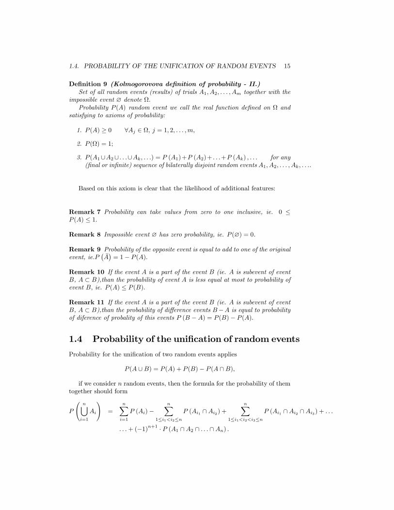
1.4 Probability of the uni�cation of random events
Probability for the uni�cation of two random events applies
P (A [B) = P (A) + P (B)� P (A \B);
if we consider n random events, then the formula for the probability of themtogether should form
P
n[i=1
Ai
!=
nXi=1
P (Ai)�nX
1�i1<i2�nP (Ai1 \Ai2) +
nX1�i1<i2<i3�n
P (Ai1 \Ai2 \Ai3) + : : :
: : :+ (�1)n+1 � P (A1 \A2 \ : : : \An) :
16 CHAPTER 1. PROBABILITY THEORY
Remark 12 Previous relationship is at �rst glance seem incomprehensible, butfor speci�c values of n (most used values are 2, 3 or 4) becomes considerablymore comprehensible
i) P (A[B [C) = P (A) +P (B) +P (C)�P (A\B)�P (A\C)�P (B \C)+
+P (A \B \ C);
ii) P (A [B [ C [D) = P (A) + P (B) + P (C) + P (D)�
�P (A\B)�P (A\C)�P (A\D)�P (B \C)�P (B \D)�P (C \D)+
+P (A \B \ C) + P (A \B \D) + P (A \ C \D) + P (B \ C \D)�
�P (A \B \ C \D):
Consequence 1 Consider the ending of the relationship for the uni�cation ofdisjoint events, ie. if Ai \Aj = ? for i 6= j, than
P
n[i=1
Ai
!=
nXi=1
P (Ai) :
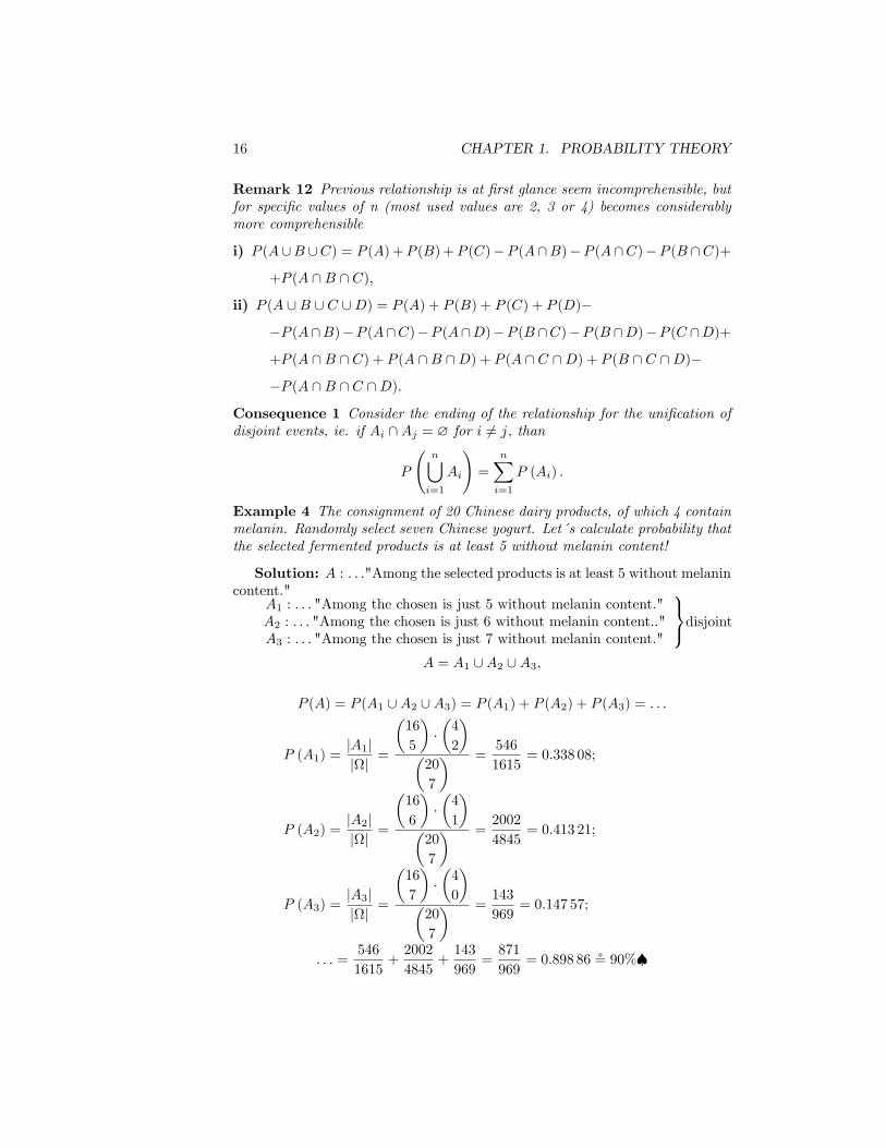
Example 4 The consignment of 20 Chinese dairy products, of which 4 containmelanin. Randomly select seven Chinese yogurt. Let´ s calculate probability thatthe selected fermented products is at least 5 without melanin content!
Solution: A : : : :"Among the selected products is at least 5 without melanincontent."
A1 : : : : "Among the chosen is just 5 without melanin content."A2 : : : : "Among the chosen is just 6 without melanin content.."A3 : : : : "Among the chosen is just 7 without melanin content."
9=;disjointA = A1 [A2 [A3;
P (A) = P (A1 [A2 [A3) = P (A1) + P (A2) + P (A3) = : : :
P (A1) =jA1jjj =
�16
5
���4
2
��20
7
� =546
1615= 0:338 08;
P (A2) =jA2jjj =
�16
6
���4
1
��20
7
� =2002
4845= 0:413 21;
P (A3) =jA3jjj =
�16
7
���4
0
��20
7
� =143
969= 0:147 57;
: : : =546
1615+2002
4845+143
969=871
969= 0:898 86 $ 90%�
1.5. PROBALITY OF THE OPPOSITE EVENT 17
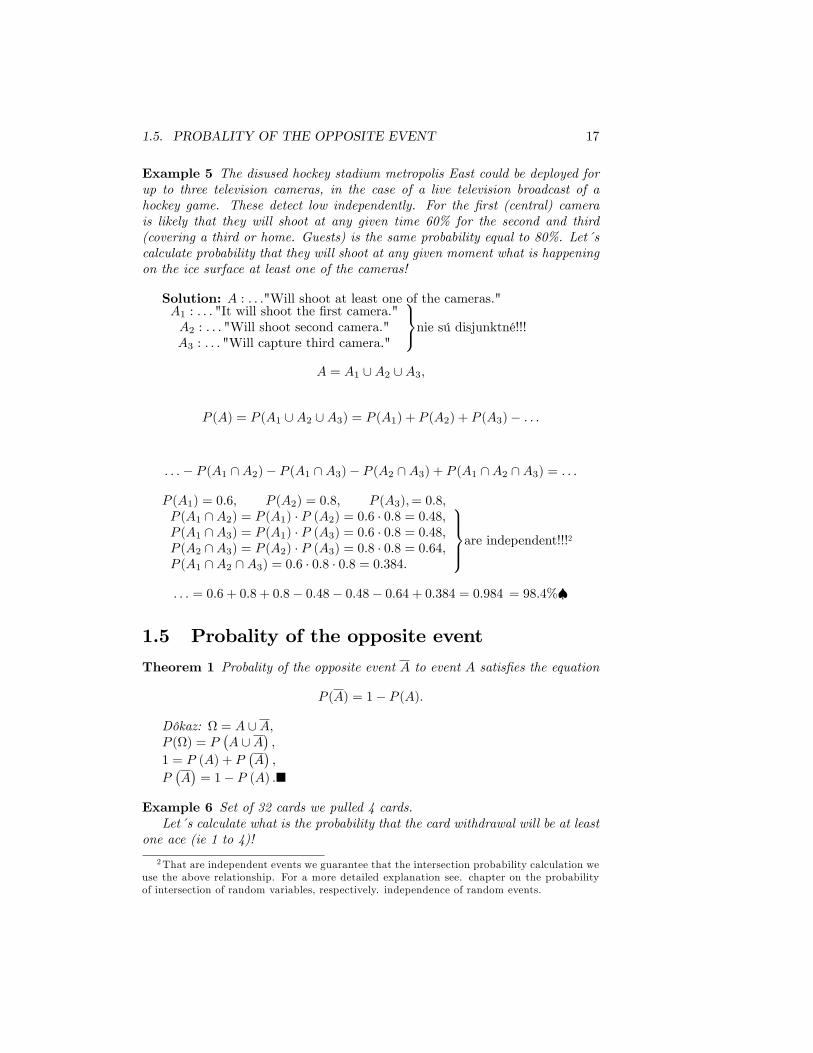
Example 5 The disused hockey stadium metropolis East could be deployed forup to three television cameras, in the case of a live television broadcast of ahockey game. These detect low independently. For the �rst (central) camerais likely that they will shoot at any given time 60% for the second and third(covering a third or home. Guests) is the same probability equal to 80%. Let´ scalculate probability that they will shoot at any given moment what is happeningon the ice surface at least one of the cameras!
Solution: A : : : :"Will shoot at least one of the cameras."A1 : : : : "It will shoot the �rst camera."A2 : : : : "Will shoot second camera."A3 : : : : "Will capture third camera."
9=;nie sú disjunktné!!!A = A1 [A2 [A3;
P (A) = P (A1 [A2 [A3) = P (A1) + P (A2) + P (A3)� : : :
: : :� P (A1 \A2)� P (A1 \A3)� P (A2 \A3) + P (A1 \A2 \A3) = : : :
P (A1) = 0:6; P (A2) = 0:8; P (A3);= 0:8;P (A1 \A2) = P (A1) � P (A2) = 0:6 � 0:8 = 0:48;P (A1 \A3) = P (A1) � P (A3) = 0:6 � 0:8 = 0:48;P (A2 \A3) = P (A2) � P (A3) = 0:8 � 0:8 = 0:64;P (A1 \A2 \A3) = 0:6 � 0:8 � 0:8 = 0:384:
9>>=>>;are independent!!!2: : : = 0:6 + 0:8 + 0:8� 0:48� 0:48� 0:64 + 0:384 = 0:984 = 98:4%�
1.5 Probality of the opposite event
Theorem 1 Probality of the opposite event A to event A satis�es the equation
P (A) = 1� P (A):
Dôkaz: = A [A;P () = P
�A [A
�;
1 = P (A) + P�A�;
P�A�= 1� P (A) :�
Example 6 Set of 32 cards we pulled 4 cards.Let´ s calculate what is the probability that the card withdrawal will be at least
one ace (ie 1 to 4)!
2That are independent events we guarantee that the intersection probability calculation weuse the above relationship. For a more detailed explanation see. chapter on the probabilityof intersection of random variables, respectively. independence of random events.
18 CHAPTER 1. PROBABILITY THEORY
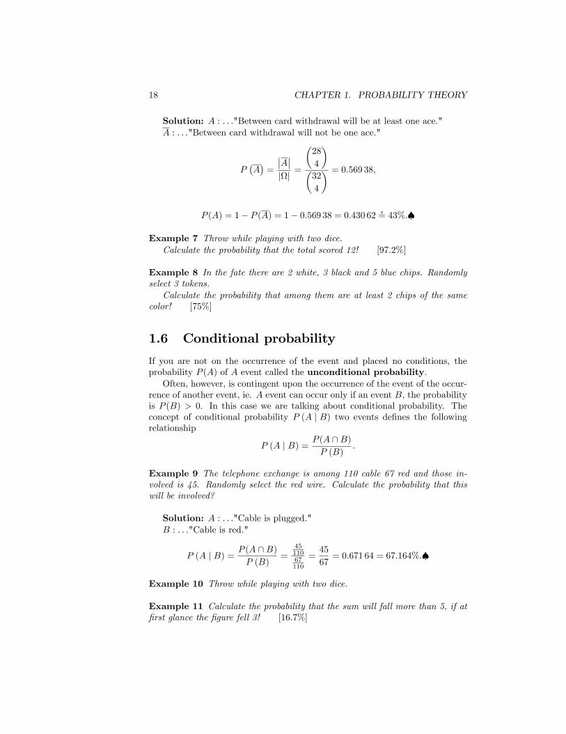
Solution: A : : : :"Between card withdrawal will be at least one ace."A : : : :"Between card withdrawal will not be one ace."
P�A�=
��A��jj =
�28
4
��32
4
� = 0:569 38;
P (A) = 1� P (A) = 1� 0:569 38 = 0:430 62 $ 43%:�
Example 7 Throw while playing with two dice.Calculate the probability that the total scored 12! [97:2%]
Example 8 In the fate there are 2 white, 3 black and 5 blue chips. Randomlyselect 3 tokens.Calculate the probability that among them are at least 2 chips of the same
color! [75%]
1.6 Conditional probability
If you are not on the occurrence of the event and placed no conditions, theprobability P (A) of A event called the unconditional probability.Often, however, is contingent upon the occurrence of the event of the occur-
rence of another event, ie. A event can occur only if an event B, the probabilityis P (B) > 0. In this case we are talking about conditional probability. Theconcept of conditional probability P (A j B) two events de�nes the followingrelationship
P (A j B) = P (A \B)P (B)
:
Example 9 The telephone exchange is among 110 cable 67 red and those in-volved is 45. Randomly select the red wire. Calculate the probability that thiswill be involved?
Solution: A : : : :"Cable is plugged."B : : : :"Cable is red."
P (A j B) = P (A \B)P (B)
=4511067110
=45
67= 0:671 64 = 67:164%:�
Example 10 Throw while playing with two dice.
Example 11 Calculate the probability that the sum will fall more than 5, if at�rst glance the �gure fell 3! [16:7%]
1.7. INTERSECTION PROBABILITY OF RANDOM PHENOMENA 19
1.7 Intersection probability of random phenom-ena
For intersection probability of random phenomena A1; A2; : : : ; An applies
P
n\i=1
Ai
!= P (A1) � P (A2 j A1) � P (A3 j A1 \A2) � : : : � P
A3 j
n�1\i=1
Ai
!:
In the special case of the intersection of two events A and B, ie. case if theseevent occur simultaneously true that the probability of intersection is equalprobability of one of the events times the conditional probability of the secondevent
P (A \B) = P (A) � P (B j A) = P (B) � P (A j B) :
Similarly we could de�ne the probability of three events
P (A1 \A2 \A3) = P (A1) � P (A2 j A1) � P (A3 j A1 \A2) :
Event A and B will be called independent events if the occurrence ofevents and event depend on the occurrence of the event of B and B while theincidence of the event does not depend on the occurrence of event A.
Due to the previous it is clear that for independent events A and B holds3
P (A j B) = P (A) ;
P (B j A) = P (B) :
For intersection of independent events will probably be the following rela-tionship
P
n\i=1
Ai
!= P (A1) � P (A2) � P (A3) � : : : � P (An) :
Example 12 The fates are 3 white, 5 red and 7 blue balls. Randomly selectfour balls in a row.What is the probability that 1 ball will be white, 2 red, 3 red and 4 blue?
Solution: A : : : :"1. white, 2 red, 3 red, 4 blue".A1 : : : :"1. white",A2 : : : :"2. red",A3 : : : :"3. red",A4 : : : :"4. blue".
A = A1 \A2 \A3 \A4
P (A1\A2\A3\A4) = P (A1)�P (A2 j A1)�P (A3 j A1 \A2)�P (A4 j A1 \A2 \A3) =3Once again, however, stressed that this applies only if they are independent event.
20 CHAPTER 1. PROBABILITY THEORY
P (A1) =jAjjj =
�3
1
��15
1
� = 3
15=1
5;
P (A2 j A1) =5
14;
P (A3 j A1 \A2) =4
13;
P (A4 j A1 \A2 \A3) =7
12;
: : : =1
5� 514� 413� 712=1
78:�
Example 13 Labourer serves three devices, which operate independently. Theprobability that the machine does not need within one hour of intervention isequal to the �rst machinery 90%, the 2nd machine and 80% in the third 85% ofthe machine.What is the probability that one hour will require the intervention of workers
or one machine?
Solution: A : : : :"For one hour will require the intervention of workers orone machine"A1 : : : :"For one hour will not need workers hit �rst machine",A2 : : : :"For one hour will not need workers hit second machine",A3 : : : :"For one hour will not need workers hit third machine".
A = A1 \A2 \A3;
P (A) = P (A1) � P (A2) � P (A3) = 0:9 � 0:8 � 0:85 $ 0; 61 = 61%:�
Example 14 We have three shipments of a product. The �rst shipment con-tains 8 good and 3 defective products. The second consignment contains 10 goodand 5 bad product. Third consignment contains 7 good and 4 defective prod-ucts. For each shipment we choose (independently), one product. Calculate theprobability that all three selected products are safe! [30:8%]
Example 15 V osudí sú 3 modré, 4 µcervené a 5 bielych guliµciek. Náhodnevyberieme 5 guliµciek po sebe (vyberáme po sebe a nevkladáme naspä ,t, a tedakaµzdý výber je závislý na predchádzajúcom). Vypoµcítajte pravdepodobnos ,t, µze 1.guliµcka bude biela, 2. biela, 3. µcervená, 4. µcervená a 5. modrá! [0:758%]
1.8 Full probability formula
First we de�ne the notion of a complete system of events.
1.8. FULL PROBABILITY FORMULA 21
De�nition 10 The complete system of events is called system of events H1;H2; : : : ;Hn,which are by two disjoint, ie. Hi \Hj = ? for i 6= j, while their union is thecertain events, ie. H1 [H2 [ : : : [Hn = :
Consequence 2 While events H1;H2; : : : ;Hn form a complete system of events,then the probality of any event and can be determined using what is known asfull probability formula
P (A) =nXi=1
P (Hi) � P (A j Hi) (Full probability formula)
or else
P (A) = P (H1) � P (A j H1) + P (H2) � P (A j H2) + : : :+ P (Hn) � P (A j Hn) :
The formula is the culmination of a clear de�nition full probability, whereany event which is fully distributed in complete system of events to disjointparts, which, since the system is complete, uni�cation gives us the whole eventA.
Remark 13 Full probability formula is true if we replace n by in�nite, ie. n!1.
Remark 14 Events H1;H2; : : : ;Hn commonly we called a hypothesis and applyfor them
P (H1) + P (H2) + : : :+ P (Hn) = 1:
Example 16 Come into the store three production companies of the same typeproducts represented 2:3:4. Probability of a �awless product is �rst holding 82%of 2 holding 93% and 90% of 3.podniku.What is the probability that a �awless product we buy?
Solution: A : : : :"We buy a perfect product."Hi : : : :"The product is the i-th company."
P (A) = P (H1) � P (A j H1) + P (H2) � P (A j H2) + P (H3) � P (A j H3) =
=2
9� 0:82 + 3
9� 0:93 + 4
9� 0:9 $ 0:892 = 89:2%�
Example 17 Two consignments containing products. The �rst shipment con-tains 18 good and 3 bad. The second shipment includes 9 good and 1 bad. Thesecond consignment choose a product and give it to �rst. Then randomly selectone product from the �rst shipment.Let´ s calculate probability that this is good!
Solution: A : : : :"The product is good."H1 : : : :"The product is the second shipment is defective."H2 : : : :"The product is the second shipment is good."
P (A) = P (H1) � P (A j H1) + P (H2) � P (A j H2) =1
10� 1822+9
10� 1922= 85:9%�
22 CHAPTER 1. PROBABILITY THEORY
Example 18 Until fate with three balls to put a white ball. Assume that anynumber of white balls in fate is likely. Then drawn at random from pulled oneball.How likely is it white?
Solution: A : : : :"The selected ball is white."H1 : : : :"In the original fates are all three white balls."H2 : : : :"In the original fates are two white balls."H3 : : : :"In the initial fate is a white ball."H4 : : : :"In the initial fate is no white ball. "
P (A) = P (H1) � P (A j H1) + P (H2) � P (A j H2) +P (H3) � P (A j H3) + P (H4) � P (A j H4)
=1
4� 1 + 1
4� 34+1
4� 24+1
4� 14=5
8= 0:625 = 62:5%�
Example 19 Three plants produced bulbs.The �rst one covers 60% of all consumption region, the second covers 25%
and third 15%.Of every 100 �rst-tales factory default is 92, of 2 race 78 and of 3 their
factory is only 63 standard.Calculate what is the probability that the bulb was purchased in this region is
the standard! [84:1%]
Example 20 Two consignments containing products. The �rst shipment con-tains 18 good and 3 bad. The second shipment includes 9 good and 1 bad. Thesecond consignment choose 2 products and let him into the �rst. Then randomlyselect one product from the �rst shipment.Calculate probability that this is good! [86:1%]
1.9 Bayesov vzorec
Let events H1;H2; : : : ;Hn form a complete system of events. If a result ofrandom trial is an event A, then the conditional probability of event Hj withrespect to event A we calculat by using Bayes formula
P (Hj j A) =P (Hj) � P (A j Hj)
P (A)=
P (Hj) � P (A j Hj)nPi=1
P (Hi) � P (A j Hi):
Remark 15 A is known event that occurs when by a random experiment. Bayesformula refers to the probability of hypotheses, provided that the event occurs A.
Remark 16 Bayes formula is true also if we replace n in�nite, ie.
1.10. BERNOULLIHO VZOREC 23
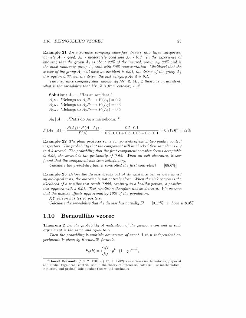
Example 21 An insurance company classi�es drivers into three categories,namely A1 - good, A2 - moderately good and A3 - bad. In the experience ofknowing that the group A1 is about 20% of the insured, group A2 30% and isthe most numerous group A3 with with 50% representation. Likelihood that thedriver of the group A1 will have an accident is 0.01, the driver of the group A2this option 0:03, but the driver the last category A3 it is 0.1.The insurance company shall indemnify Mr. Z. Mr. Z then has an accident,
what is the probability that Mr. Z is from category A3?
Solution: A : : : :"Has an accident."A1:. . . "Belongs to A1:" ! P (A1) = 0:2A2:. . . "Belongs to A2:" ! P (A2) = 0:3A3:. . . "Belongs to A3:" ! P (A3) = 0:5
A3 j A : : : :"Patrí do A3 a má nehodu. "
P (A3 j A) =P (A3) � P (A j A3)
P (A)=
0:5 � 0:10:2 � 0:01 + 0:3 � 0:03 + 0:5 � 0:1 = 0:819 67 = 82%
Example 22 The plant produces some components of which two quality controlinspectors. The probability that the component will be checked �rst sampler is 0.7to 0.3 second. The probability that the �rst component sampler deems acceptableis 0.92, the second is the probability of 0.98. When an exit clearance, it wasfound that the component has been satisfactory.Calculate the probability that it controlled the �rst controller! [68:6%]
Example 23 Before the disease breaks out of its existence can be determinedby biological tests, the outcome is not entirely clear. When the sick person is thelikelihood of a positive test result 0.999, contrary to a healthy person, a positivetest appears with a 0.01. Test condition therefore not be detected. We assumethat the disease a¤ects approximately 10% of the population.XY person has tested positive.Calculate the probability that the disease has actually Z! [91:7%; ie. hope is 8:3%]
1.10 Bernoulliho vzorec
Theorem 2 Let the probability of realization of the phenomenon and in eachexperiment is the same and equal to p.Then the probability k-multiple occurrence of event A in n independent ex-
periments is given by Bernoulli4 formula
Pn(k) =
�n
k
�� pk � (1� p)n�k ;
4Daniel Bernoulli (* 8. 2. 1700 � y 17. 3. 1782) was a Swiss mathematician, physicistand medic. Signi�cant contribution in the theory of di¤erential calculus, like mathematical,statistical and probabilistic number theory and mechanics.
24 CHAPTER 1. PROBABILITY THEORY
or, if we put q = 1� p (ie. probability of the opposite event), then
Pn(k) =
�n
k
�� pk � qn�k:
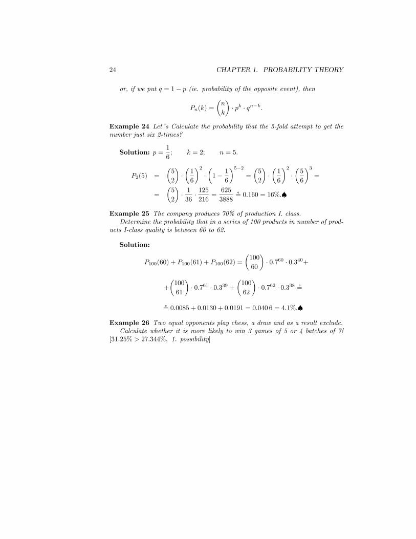
Example 24 Let´ s Calculate the probability that the 5-fold attempt to get thenumber just six 2-times?
Solution: p =1
6; k = 2; n = 5:
P2(5) =
�5
2
���1
6
�2��1� 1
6
�5�2=
�5
2
���1
6
�2��5
6
�3=
=
�5
2
�� 136� 125216
=625
3888$ 0:160 = 16%:�
Example 25 The company produces 70% of production I. class.Determine the probability that in a series of 100 products in number of prod-
ucts I-class quality is between 60 to 62.
Solution:
P100(60) + P100(61) + P100(62) =
�100
60
�� 0:760 � 0:340+
+
�100
61
�� 0:761 � 0:339 +
�100
62
�� 0:762 � 0:338 $
$ 0:0085 + 0:0130 + 0:0191 = 0:040 6 = 4:1%:�
Example 26 Two equal opponents play chess, a draw and as a result exclude.Calculate whether it is more likely to win 3 games of 5 or 4 batches of 7!
[31:25% > 27:344%; 1. possibility]
Chapter 2
Random variable
Sometimes it is useful to describe the random phenomenon by using some ofits numerical characteristics (eg size, weight, number of features, rates, etc..),which we call the random variable.
De�nition 11 Concept of random variable denote variable whose value is de-termined by the result of an accidental experiment. Repeat the experiment occursdue to changes in random processes random variable and its value can not be de-termined before carrying out the experiment, and therefore is a random variablespeci�ed probability distribution.
Random variable we denote as �1 and its value as small Arabic letters eg.x, y, z etc..
Remark 17 Sometimes it is the practice of random variables labeled in capitalletters, for example X, Y , Z and its values with corresponding lowercase ie.x, y, z: However, inattention are often confused with the variable value (ie.lowercase with capital letter), and therefore we will stick to the next sign �1, �2,�3 etc..
Remark 18 Symbol P ( = x) (resp. P ( < x)) will mean the probability ofsuch random variable takes the value of x (or enter into a value less than x).
2.1 Discrete probability distribution
De�nition 12 We say that a random variable has a discrete probability dis-tribution, if there is a �nal or countable set of real numbers fx1; x2; x3; :::g, suchthat pays
1Xi=1
P (�i = x) = 1:
1 small Greek letter "xi"
25
26 CHAPTER 2. RANDOM VARIABLE
Probability distribution random variable is given values and probabilitieswith which these values shall!
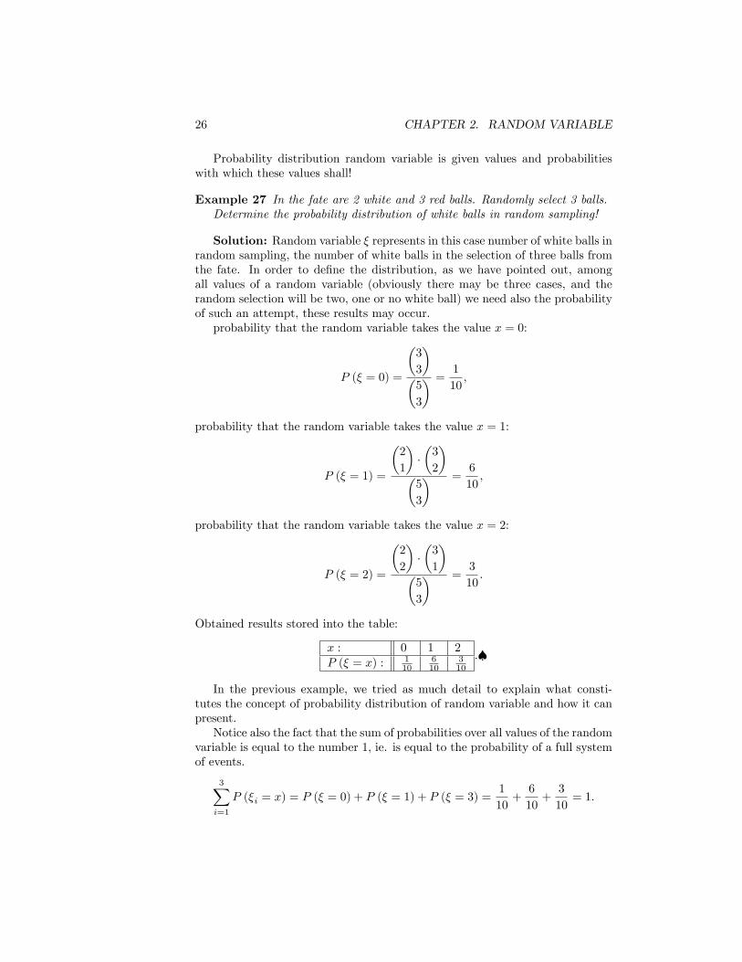
Example 27 In the fate are 2 white and 3 red balls. Randomly select 3 balls.Determine the probability distribution of white balls in random sampling!
Solution: Random variable � represents in this case number of white balls inrandom sampling, the number of white balls in the selection of three balls fromthe fate. In order to de�ne the distribution, as we have pointed out, amongall values of a random variable (obviously there may be three cases, and therandom selection will be two, one or no white ball) we need also the probabilityof such an attempt, these results may occur.probability that the random variable takes the value x = 0:
P (� = 0) =
�3
3
��5
3
� = 1
10;
probability that the random variable takes the value x = 1:
P (� = 1) =
�2
1
���3
2
��5
3
� =6
10;
probability that the random variable takes the value x = 2:
P (� = 2) =
�2
2
���3
1
��5
3
� =3
10:
Obtained results stored into the table:
x : 0 1 2P (� = x) : 1
10610
310
:�
In the previous example, we tried as much detail to explain what consti-tutes the concept of probability distribution of random variable and how it canpresent.Notice also the fact that the sum of probabilities over all values of the random
variable is equal to the number 1, ie. is equal to the probability of a full systemof events.
3Xi=1
P (�i = x) = P (� = 0) + P (� = 1) + P (� = 3) =1
10+6
10+3
10= 1:
2.2. DISTRIBUTION FUNCTION OF RANDOM VARIABLE 27
2.2 Distribution function of random variable
De�nition 13 Let the random variable be de�ned on probability space (; �; P ) :Then the real function:
F (x) = P (� < x) ; pre x 2 (�1;1) ;
is called the distribution function of random variable.
Remark 19 Distribution function of random variable is a function
i) non-decreasing,
ii) left continuous,
iii) satis�es: limx!�1
F (x) = 0 and limx!1
F (x) = 1:
Example 28 Throw a coin three times.For the random variable , which represents the number of coins �t the char-
acter side up, and we determine the probability distribution then the distributionfunction.
Solution: Probability distribution can be determined similarly as in theprevious example using Bernoulli�s formula. Results are entered in the tablebelow which are referred to the calculations.
x : 0 1 2 3P (� = x) : 1
838
38
18
P (� = 0) = P3(0) =
�3
0
�� p0 � (1� p)3 = : : :
probability of falling character is probably p = 0:5 = 12
: : : =
�3
0
���1
2
�0��1
2
�3=1
8;
P (� = 1) = P3(1) =
�3
1
���1
2
�1��1
2
�2=3
8;
P (� = 2) = P3(2) =
�3
2
���1
2
�2��1
2
�1=3
8;
P (� = 3) = P3(3) =
�3
3
���1
2
�3��1
2
�0=1
8:
Distribution function can be determined at intervals de�ned by the values ofrandom variablex < 0 : F (x) = P (� < 0) = 0 (impossible event),
28 CHAPTER 2. RANDOM VARIABLE
0 � x < 1 : F (x) = P (� < 1) = P (� = 0) =1
8;
1 � x < 2 : F (x) = P (� < 2) = P [(� = 0) [ (� = 1)] == P (� = 0) + P (� = 1) =
1
8+3
8=4
8;
2 � x < 3 : F (x) = P (� < 3) = P [(� = 0) [ (� = 1) [ (� = 2)] == P (� = 0) + P (� = 1) + P (� = 2) =
=1
8+3
8+3
8=7
8;
3 � x : F (x) = P [(� = 0) [ (� = 1) [ (� = 2) [ (� = 3)] == P (� = 0) + P (� = 1) + P (� = 2) + P (� = 3) =
=1
8+3
8+3
8+1
8= 1:
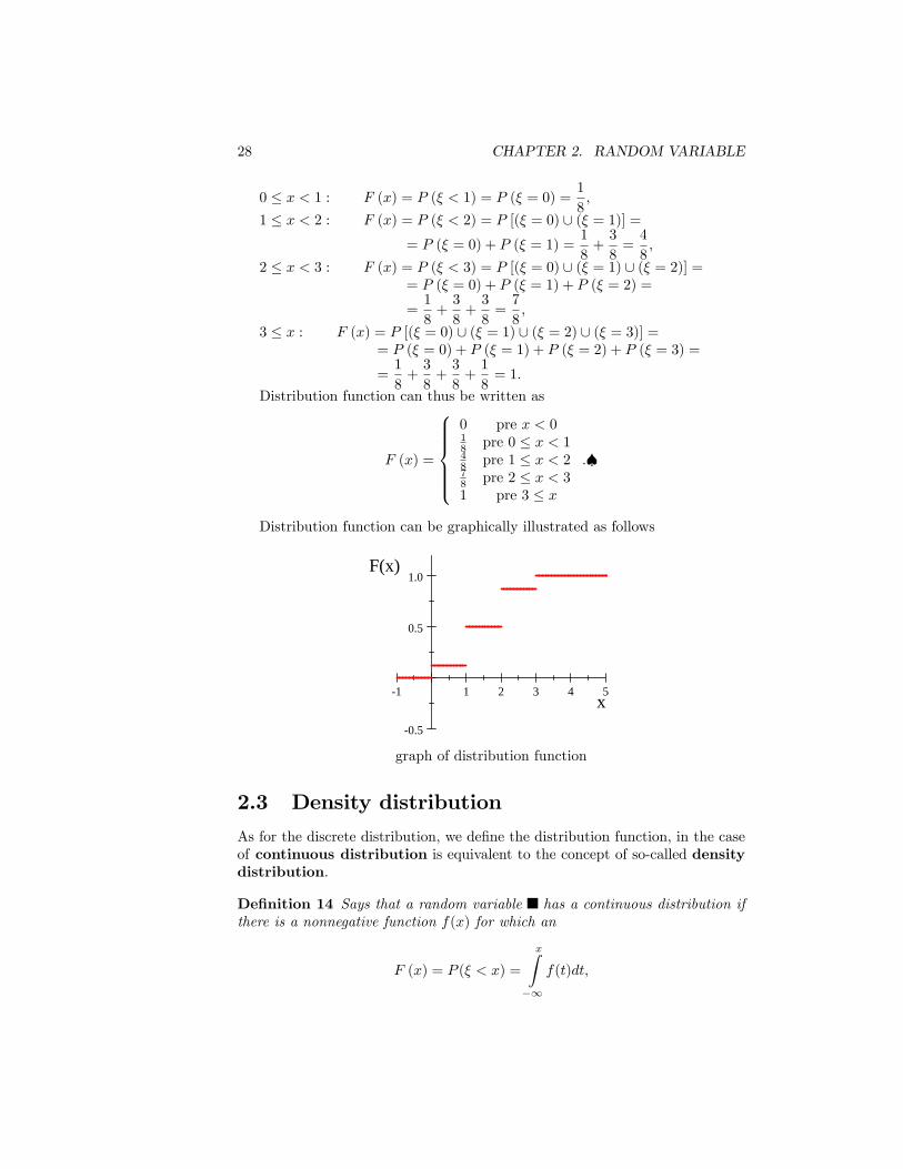
Distribution function can thus be written as
F (x) =
8>>>><>>>>:0 pre x < 018 pre 0 � x < 148 pre 1 � x < 278 pre 2 � x < 31 pre 3 � x
:�
Distribution function can be graphically illustrated as follows
1 1 2 3 4 5
0.5
0.5
1.0
x
F(x)
graph of distribution function
2.3 Density distribution
As for the discrete distribution, we de�ne the distribution function, in the caseof continuous distribution is equivalent to the concept of so-called densitydistribution.
De�nition 14 Says that a random variable has a continuous distribution ifthere is a nonnegative function f(x) for which an
F (x) = P (� < x) =
xZ�1
f(t)dt;
2.3. DENSITY DISTRIBUTION 29
where F (x) is the distribution function pertaining random variable .Function f(x) is called the probability distribution density of random variable
.
Remark 20 Previous relation clearly determines the density distribution. Ifthat is the distribution density function f(x) continuous everywhere (ie the in-terval (�1;1)), we can also de�ne the relationship
f(x) = F 0 (x) :
Remark 21 If the density distribution f (x) everywhere continuous function, isthe distribution function F (x) everywhere continuous function.
2.3.1 Basic features of the density distribution.
F (b)� F (a) =bZa
f(x)dx;
from where directly derives important relationships for calculating the prbabilityof a random variable which has continuous distribution
P (a < � < b) =
bZa
f(x)dx = F (b)� F (a);
P (a � � < b) =
bZa
f(x)dx = F (b)� F (a);
P (a < � � b) =bZa
f(x)dx = F (b)� F (a);
P (a � � � b) =bZa
f(x)dx = F (b)� F (a):
In the previous formulas we have seen that the calculation of de�nite integral toour border points do not matter and therefore it does not matter whetherthe relations we use a sharp or blurred inequality.
1Z�1
f(x)dx = 1:
This relationship is sort of the equivalent relation1Xi=1
P (�i = x) = 1 for
discrete random variable distribution.
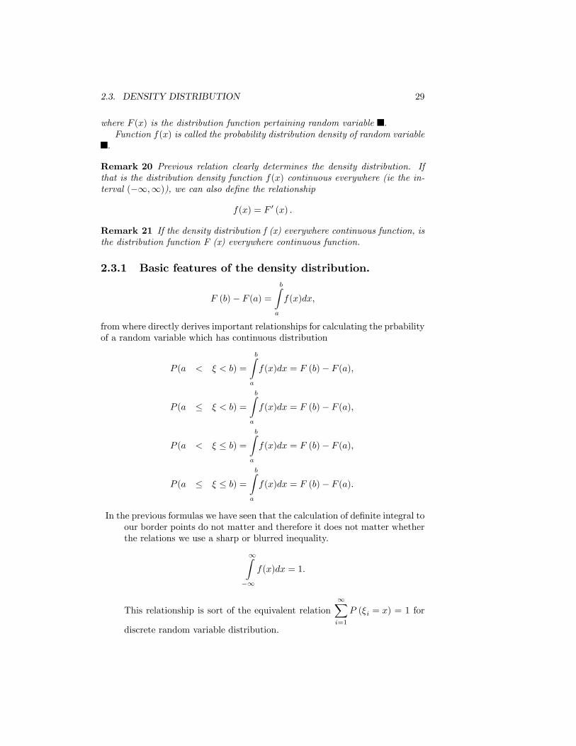
30 CHAPTER 2. RANDOM VARIABLE
Graphically it means, that the area between the x-axis and the densityfunction is equal to 1.
x
f(x)
Density distribution
When calculating the probability that a random variable will be included insuch interval h�1; 2i, we calculated the de�nite integral
P (�1 � � � 2) =2Z
�1
f(x)dx;
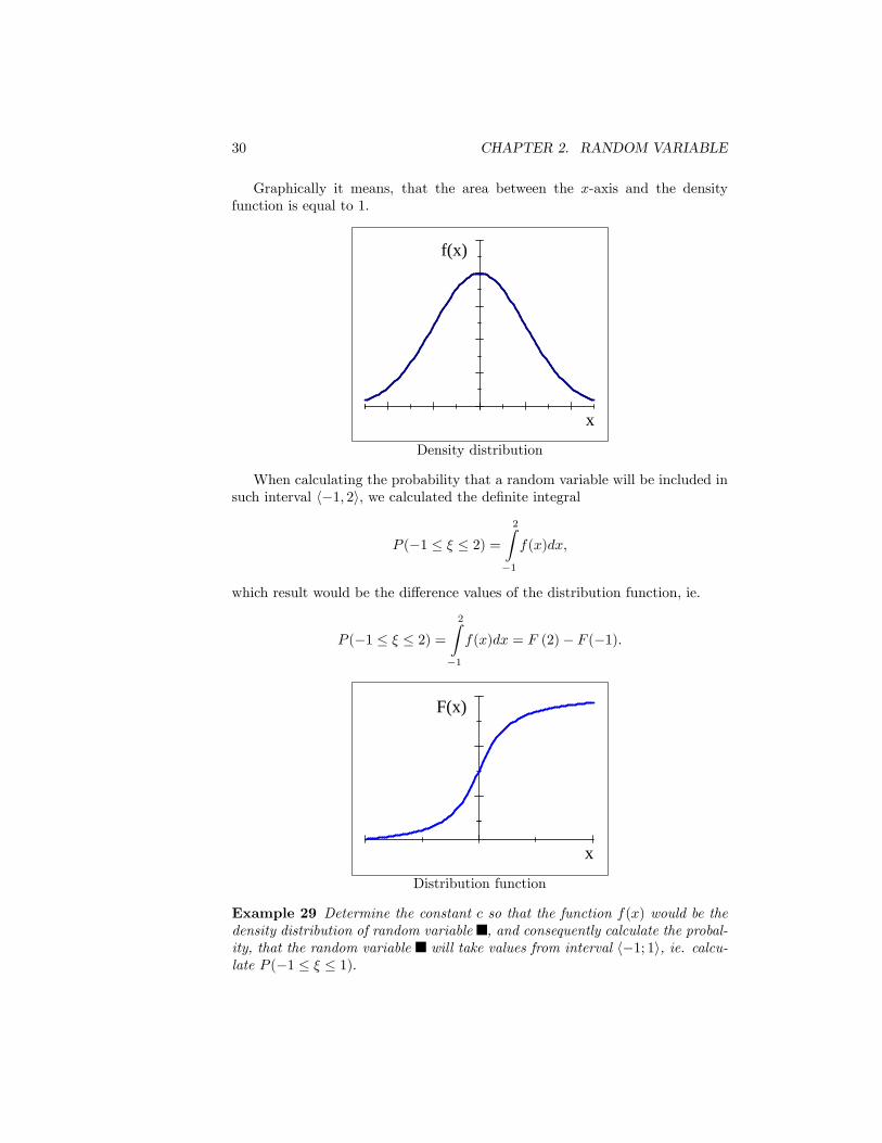
which result would be the di¤erence values of the distribution function, ie.
P (�1 � � � 2) =2Z
�1
f(x)dx = F (2)� F (�1):
x
F(x)
Distribution function
Example 29 Determine the constant c so that the function f(x) would be thedensity distribution of random variable , and consequently calculate the probal-ity, that the random variable will take values from interval h�1; 1i, ie. calcu-late P (�1 � � � 1):
2.4. NUMERICAL CHARACTERISTICS OF RANDOM VARIABLE 31
f(x) =
�cx2 � e�x3 x � 0
0 x < 0:
Solution: Must satisfy
1Z�1
f(x)dx = 1:
1Z0
f(x)dx =
1Z0
cx2 � e�x3
dx = c �1Z0
x2 � e�x3
dx =
, t = x3
dt = 3x2dx0! 01!1
,=
=c
3
1Z0
e�tdt =c
3
��e�t
�10=c
3
�0 + e0
�10=c
3;
and thereforec
3= 1:
Thus, where truec = 3:
Density distribution will thus in shape
f(x) =
�3x2 � e�x3 ; x � 0;
0; x < 0:
Probability P (�1 � � � 1) we calculate as follows
P (�1 � � � 1) =1Z
�1
f(x)dx = 0 +
1Z0
f(x)dx =
=
1Z0
3x2 � e�x3
dx =��e�1 + e0
�= �1
e+ 1 $ 0:632 = 63:2%:�
2.4 Numerical characteristics of random vari-able
Distribution function, probability distribution and density distribution accu-rately describe the likelihood of conduct random variable. In practice, we oftenused certain numeric characteristics to describe a random variable.
2.4.1 Mean value
Mean value of random variable is a kind of "location characteristic". We canseen at it as a "center" of the probability distribution, which is centered aroundall the values of random variable . Oznaµcujeme ju E(�) alebo �:Mean value is for:
32 CHAPTER 2. RANDOM VARIABLE
1. discrete random variable and its probability function pi de�ned as
E(�) =nXi=1
xi � pi;
continuous random variable and its probability density f(x) de�ned as
E(�) =
1Z�1
x � f(x)dx:
Properties of mean value
i) E(c) = c, where c is constant,
ii) E(a � � + b) = a � E(�) + b, where a; b are constants,
iii) E(�1 + �2 + : : :+ �n) = E(�1) + E(�2) + : : :+ E(�n),
iv) E(�1 � �2) = E(�1) � E(�2), if the random variable �1; �2 independent.
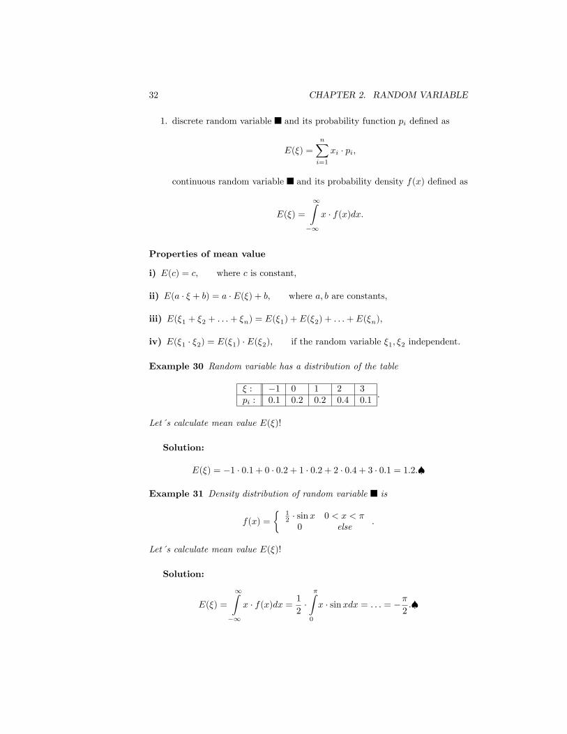
Example 30 Random variable has a distribution of the table
� : �1 0 1 2 3pi : 0:1 0:2 0:2 0:4 0:1
:
Let´ s calculate mean value E(�)!
Solution:
E(�) = �1 � 0:1 + 0 � 0:2 + 1 � 0:2 + 2 � 0:4 + 3 � 0:1 = 1:2:�
Example 31 Density distribution of random variable is
f(x) =
�12 � sinx 0 < x < �0 else
:
Let´ s calculate mean value E(�)!
Solution:
E(�) =
1Z�1
x � f(x)dx = 1
2��Z0
x � sinxdx = : : : = ��2:�
2.4. NUMERICAL CHARACTERISTICS OF RANDOM VARIABLE 33
2.4.2 Variance (dispersion) and standard deviation
Variability re�ects the variability of distribution of random variable values, their�uctuations around some constant. We will be particularly interested in howthese values scatter around the mean value. The most common expression ofthis variability is the variance (dispersion), which we signify D(�) or �2.Generally, we can the dispersion express with relation
D(�) = E�[� � E (�)]2
�;
and using the properties of the mean change in shape
D(�) = E��2�� [E (�)]2 :
Dispersion for:
1. discrete random variable is de�ned as
D(�) =nXi=1
[xi � E (�)]2 � pi;
2. continuous random variable and its probability density f(x) de�ned as
D(�) =
1Z�1
[x� E (�)]2 f(x)dx:
Dispersion characteristics
i) D(c) = 0; where c is constant,
ii) D(a � � + b) = a2 � E(�); where a; b are constants,
iii) Let the random variable �1; �2; : : : ; �n be independent, then satisfy
D(�1 + �2 + : : :+ �n) = D(�1) +D(�2) + : : :+D(�n);
D(�1 � �2 � : : :� �n) = D(�1)�D(�2)� : : :�D(�n):
Another feature of variability is the standard deviation , which is de�nedby dispersion as
� =pD(�) or �2 = D(�):
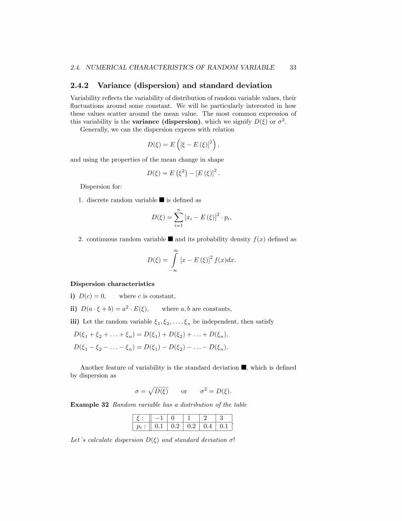
Example 32 Random variable has a distribution of the table
� : �1 0 1 2 3pi : 0:1 0:2 0:2 0:4 0:1
:
Let´ s calculate dispersion D(�) and standard deviation �!
34 CHAPTER 2. RANDOM VARIABLE
Solution:
D(�) = (�1� 1:2)2 � 0:1 + (0� 1:2)2 � 0:2 + (1� 1:2)2 � 1:2+
+ (2� 1:2)2 � 0:4 + (3� 1:2)2 � 0:1 = 1: 4;
� =pD(�) =
p1: 4 = 1: 183 2:�
Example 33 Density distribution of random variable is
f(x) =
(sinx 0 < x <
�
20 else
:
Let´ s calculate dispersion D(�) and standard deviation �; if the mean value isE(�) = a!
Solution:
D(�) =
1Z�1
(x� a)2 � f(x)dx =
�2Z0
(x� a)2 � sinxdx = : : : = a2 � 2a+ � � 2:�
Chapter 3
Signi�cant continuousdistribution of randomvariable
3.1 Normal distribution (Laplace-Gaussovo dis-tribution)
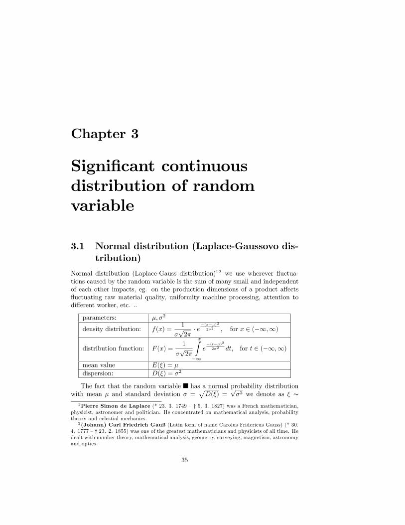
Normal distribution (Laplace-Gauss distribution)12 we use wherever �uctua-tions caused by the random variable is the sum of many small and independentof each other impacts, eg. on the production dimensions of a product a¤ects�uctuating raw material quality, uniformity machine processing, attention todi¤erent worker, etc. ..
parameters: �; �2
density distribution: f(x) =1
�p2�� e
�(x��)2
2�2 ; for x 2 (�1;1)
distribution function: F (x) =1
�p2�
xZ�1
e�(t��)2
2�2 dt; for t 2 (�1;1)
mean value E(�) = �dispersion: D(�) = �2
The fact that the random variable has a normal probability distributionwith mean � and standard deviation � =
pD(�) =
p�2 we denote as � s
1Pierre Simon de Laplace (* 23. 3. 1749 �y 5. 3. 1827) was a French mathematician,physicist, astronomer and politician. He concentrated on mathematical analysis, probabilitytheory and celestial mechanics.
2 (Johann) Carl Friedrich Gauß(Latin form of name Carolus Fridericus Gauss) (* 30.4. 1777 �y 23. 2. 1855) was one of the greatest mathematicians and physicists of all time. Hedealt with number theory, mathematical analysis, geometry, surveying, magnetism, astronomyand optics.
35
36CHAPTER 3. SIGNIFICANT CONTINUOUS DISTRIBUTIONOF RANDOMVARIABLE
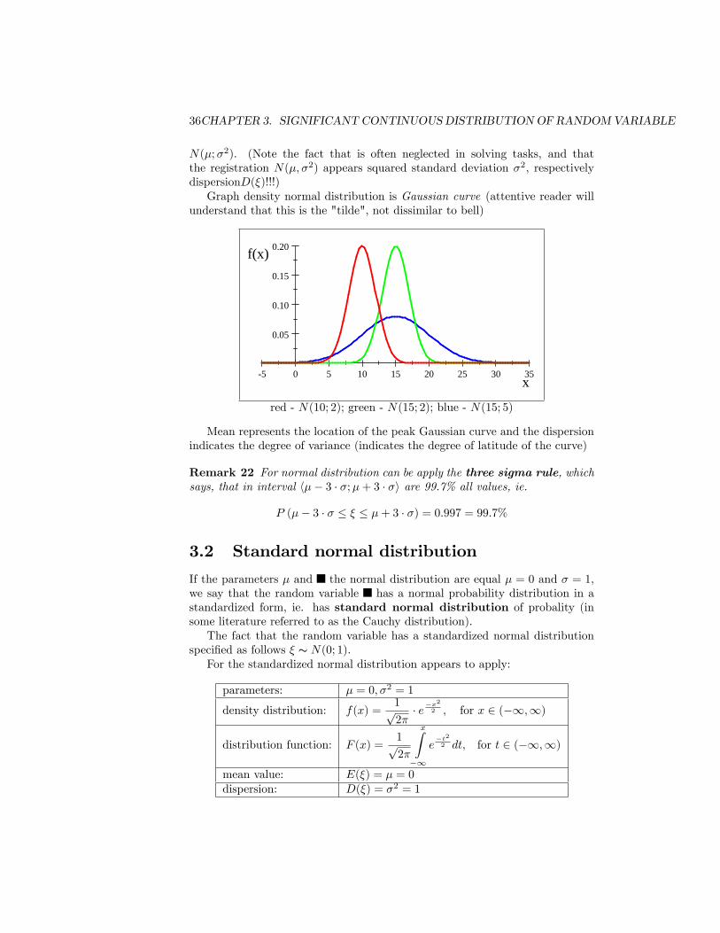
N(�;�2). (Note the fact that is often neglected in solving tasks, and thatthe registration N(�; �2) appears squared standard deviation �2, respectivelydispersionD(�)!!!)Graph density normal distribution is Gaussian curve (attentive reader will
understand that this is the "tilde", not dissimilar to bell)
5 0 5 10 15 20 25 30 35
0.05
0.10
0.15
0.20
x
f(x)
red - N(10; 2); green - N(15; 2); blue - N(15; 5)
Mean represents the location of the peak Gaussian curve and the dispersionindicates the degree of variance (indicates the degree of latitude of the curve)
Remark 22 For normal distribution can be apply the three sigma rule, whichsays, that in interval h�� 3 � �;�+ 3 � �i are 99.7% all values, ie.
P (�� 3 � � � � � �+ 3 � �) = 0:997 = 99:7%
3.2 Standard normal distribution
If the parameters � and the normal distribution are equal � = 0 and � = 1,we say that the random variable has a normal probability distribution in astandardized form, ie. has standard normal distribution of probality (insome literature referred to as the Cauchy distribution).The fact that the random variable has a standardized normal distribution
speci�ed as follows � s N(0; 1):For the standardized normal distribution appears to apply:
parameters: � = 0; �2 = 1
density distribution: f(x) =1p2�� e�x
2
2 ; for x 2 (�1;1)
distribution function: F (x) =1p2�
xZ�1
e�t22 dt; for t 2 (�1;1)
mean value: E(�) = � = 0dispersion: D(�) = �2 = 1
3.2. STANDARD NORMAL DISTRIBUTION 37
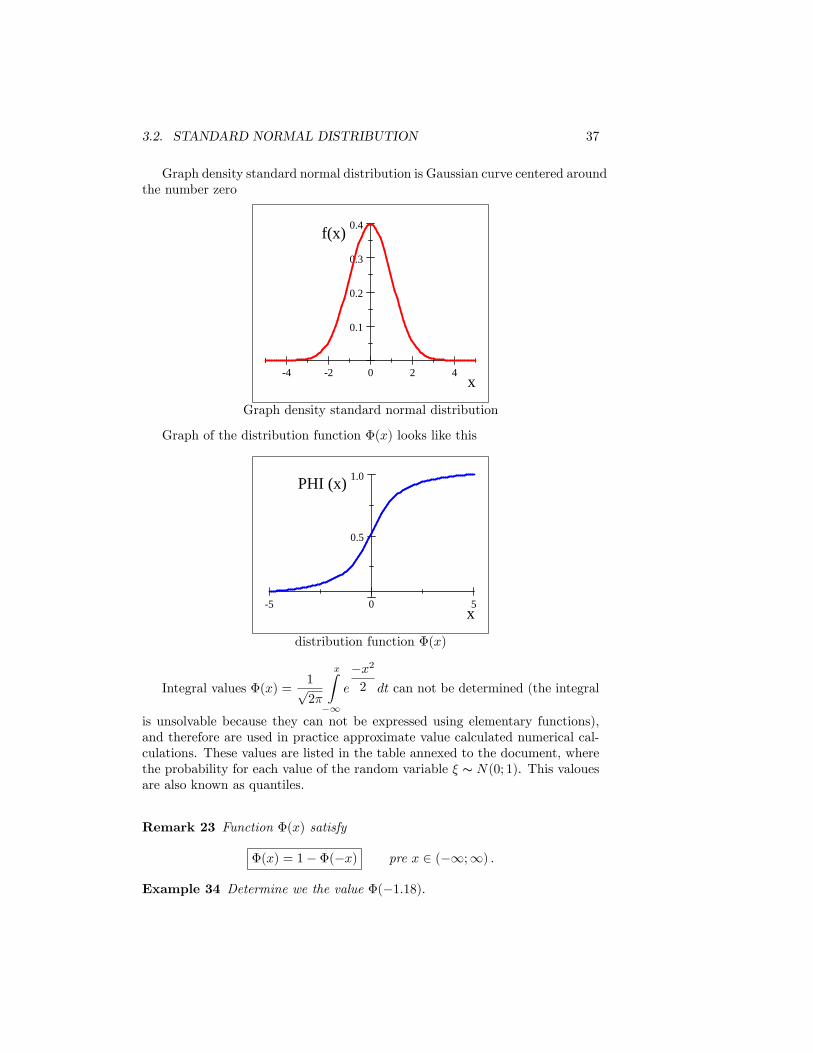
Graph density standard normal distribution is Gaussian curve centered aroundthe number zero
4 2 0 2 4
0.1
0.2
0.3
0.4
x
f(x)
Graph density standard normal distribution
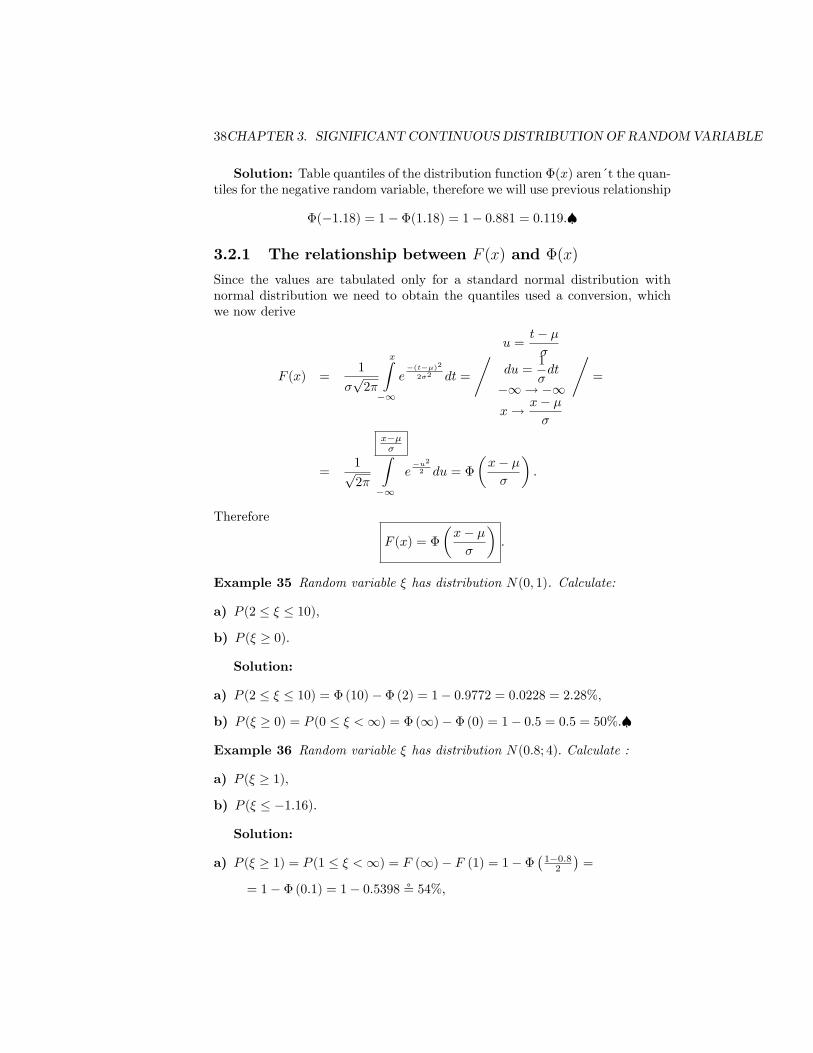
Graph of the distribution function �(x) looks like this
5 0 5
0.5
1.0
x
PHI (x)
distribution function �(x)
Integral values �(x) =1p2�
xZ�1
e
�x22 dt can not be determined (the integral
is unsolvable because they can not be expressed using elementary functions),and therefore are used in practice approximate value calculated numerical cal-culations. These values are listed in the table annexed to the document, wherethe probability for each value of the random variable � s N(0; 1). This valouesare also known as quantiles.
Remark 23 Function �(x) satisfy
�(x) = 1� �(�x) pre x 2 (�1;1) :
Example 34 Determine we the value �(�1:18):
38CHAPTER 3. SIGNIFICANT CONTINUOUS DISTRIBUTIONOF RANDOMVARIABLE
Solution: Table quantiles of the distribution function �(x) aren´t the quan-tiles for the negative random variable, therefore we will use previous relationship
�(�1:18) = 1� �(1:18) = 1� 0:881 = 0:119:�
3.2.1 The relationship between F (x) and �(x)
Since the values are tabulated only for a standard normal distribution withnormal distribution we need to obtain the quantiles used a conversion, whichwe now derive
F (x) =1
�p2�
xZ�1
e�(t��)2
2�2 dt =
, u =t� ��
du =1
�dt
�1! �1x! x� �
�
,=
=1p2�
x���Z
�1
e�u22 du = �
�x� ��
�:
Therefore
F (x) = �
�x� ��
�:
Example 35 Random variable � has distribution N(0; 1). Calculate:
a) P (2 � � � 10);
b) P (� � 0):
Solution:
a) P (2 � � � 10) = � (10)� � (2) = 1� 0:9772 = 0:0228 = 2:28%;
b) P (� � 0) = P (0 � � <1) = � (1)� � (0) = 1� 0:5 = 0:5 = 50%:�
Example 36 Random variable � has distribution N(0:8; 4): Calculate :
a) P (� � 1);
b) P (� � �1:16):
Solution:
a) P (� � 1) = P (1 � � <1) = F (1)� F (1) = 1� ��1�0:82
�=
= 1� � (0:1) = 1� 0:5398 $ 54%;
3.2. STANDARD NORMAL DISTRIBUTION 39
b) P (� � �1:16) = P (�1 < � � �1:16) = F (�1:16)� F (�1) =
= ���1:16�0:8
2
�� 0 = � (�0:98) = 1� � (�0:98) =
= 1� 0:8365 = 0:1635�
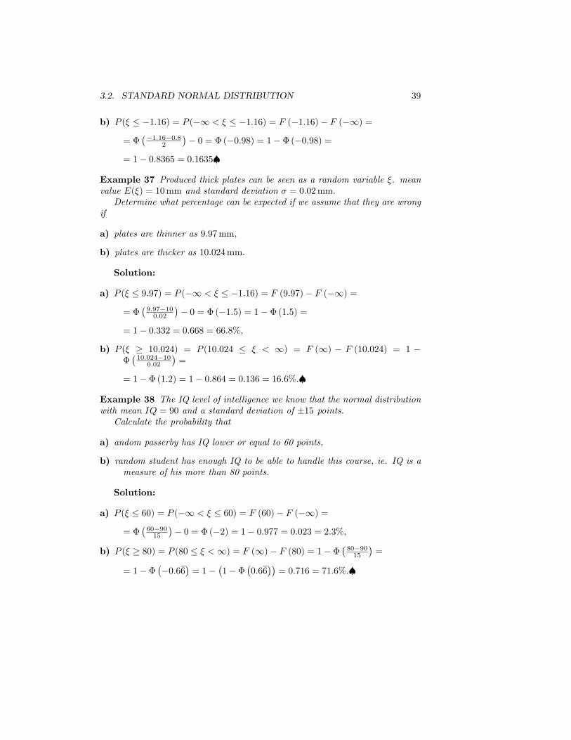
Example 37 Produced thick plates can be seen as a random variable �. meanvalue E(�) = 10mm and standard deviation � = 0:02mm:Determine what percentage can be expected if we assume that they are wrong
if
a) plates are thinner as 9:97mm;
b) plates are thicker as 10:024mm:
Solution:
a) P (� � 9:97) = P (�1 < � � �1:16) = F (9:97)� F (�1) =
= ��9:97�100:02
�� 0 = � (�1:5) = 1� � (1:5) =
= 1� 0:332 = 0:668 = 66:8%;
b) P (� � 10:024) = P (10:024 � � < 1) = F (1) � F (10:024) = 1 ���10:024�10
0:02
�=
= 1� � (1:2) = 1� 0:864 = 0:136 = 16:6%:�
Example 38 The IQ level of intelligence we know that the normal distributionwith mean IQ = 90 and a standard deviation of �15 points.Calculate the probability that
a) andom passerby has IQ lower or equal to 60 points,
b) random student has enough IQ to be able to handle this course, ie. IQ is ameasure of his more than 80 points.
Solution:
a) P (� � 60) = P (�1 < � � 60) = F (60)� F (�1) =
= ��60�9015
�� 0 = � (�2) = 1� 0:977 = 0:023 = 2:3%;
b) P (� � 80) = P (80 � � <1) = F (1)� F (80) = 1� ��80�9015
�=
= 1� ���0:66
�= 1�
�1� �
�0:66
��= 0:716 = 71:6%:�

40CHAPTER 3. SIGNIFICANT CONTINUOUS DISTRIBUTIONOF RANDOMVARIABLE
Chapter 4
Descriptive statistics
In this chapter we consider a set of statistical N scale units (random tests), forwhich we have found the value of the investigated random variable � for eachstatistical unit (random experiment), which means that we know the values xi(for i = 1; 2; : : : ; N) examined variable �.xi represents a particular value of random variable � by i-th try.
Probability distribution of values of random variable � we get by so calledsorting, ie. creating sort of classes similar statistical units (trials).Of course that is most similar to the units with the same type of random
variable being examined, but not always be classi�ed as evaluated in this way,whether because of the diversity of �le (eg, all values are di¤erent each other andtherefore the number of classes would be equal to the scope �le) or the nominalcharacteristics (subjective assessment, for example. the word). In such cases,the class represents a class representative (one speci�c value of the variable).In the case of continuous distribution of the class represented by the intervalvalues (or the center of this interval).When sorting is necessary to comply with the principle of completeness (ie,
every element must be included in any class) and the principle of clarity (ie,every element must be included in one class).
Now would be followed by a detailed description of the compilation of sta-tistical tables for the proliferation of �le extent n. This part we omit and wewill try to illustrate what most telling in the following example.
Example 39 Investigated the population of thirty apartments. Values are:3; 2; 4; 5; 2; 2; 3; 2; 4; 5; 1; 3; 4; 4; 5; 4; 1; 3; 6; 2; 3; 4; 6; 2; 3; 4; 1; 3; 5; 4.Put together a table of the probability distribution.
Solution: First highlights the basic concepts and sign:measured values xi; for i = 1; 2; : : : ; N;absolute abundance ni (how many times a character in the selection is),
41
42 CHAPTER 4. DESCRIPTIVE STATISTICS
relative abundance pi =niN;
cumulative abundance Ni =NPi=1
ni;
kumulatívna relatívna poµcetnos ,t Mi =NiN:
xi : ni : pi : Ni : Mi :
1 3 330 3 3
30
2 6 630 8 8
30
3 7 730 16 16
30
4 8 830 24 24
30
5 4 430 28 28
30
6 2 230 30 30
30P= 30
P= 1
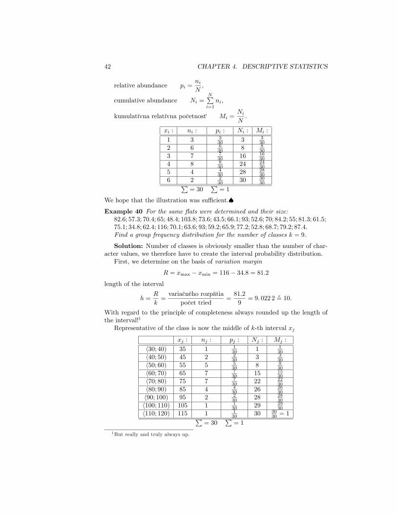
We hope that the illustration was su¢ cient.�Example 40 For the same �ats were determined and their size:82:6; 57:3; 70:4; 65; 48:4; 103:8; 73:6; 43:5; 66:1; 93; 52:6; 70; 84:2; 55; 81:3; 61:5;75:1; 34:8; 62:4; 116; 70:1; 63:6; 93; 59:2; 65:9; 77:2; 52:8; 68:7; 79:2; 87:4:Find a group frequency distribution for the number of classes k = 9.
Solution: Number of classes is obviously smaller than the number of char-acter values, we therefore have to create the interval probability distribution.First, we determine on the basis of variation margin
R = xmax � xmin = 116� 34:8 = 81:2length of the interval
h =R
k=variaµcného rozpätia
poµcet tried=81:2
9= 9: 022 2 $ 10:
With regard to the principle of completeness always rounded up the length ofthe interval!1
Representative of the class is now the middle of k-th interval xj
xj : nj : pj : Nj : Mj :
h30; 40) 35 1 130 1 1
30
h40; 50) 45 2 230 3 3
30
h50; 60) 55 5 530 8 8
30
h60; 70) 65 7 730 15 15
30
h70; 80) 75 7 730 22 22
30
h80; 90) 85 4 430 26 26
30
h90; 100) 95 2 230 28 28
30
h100; 110) 105 1 130 29 29
30
h110; 120) 115 1 130 30 30
30 = 1P= 30
P= 1
1But really and truly always up.
43
Basically it was a similar procedure as in the previous example, but please notethe index with respect to j, where j = 1; 2; : : : ; k, where k represents number ofclasses.�
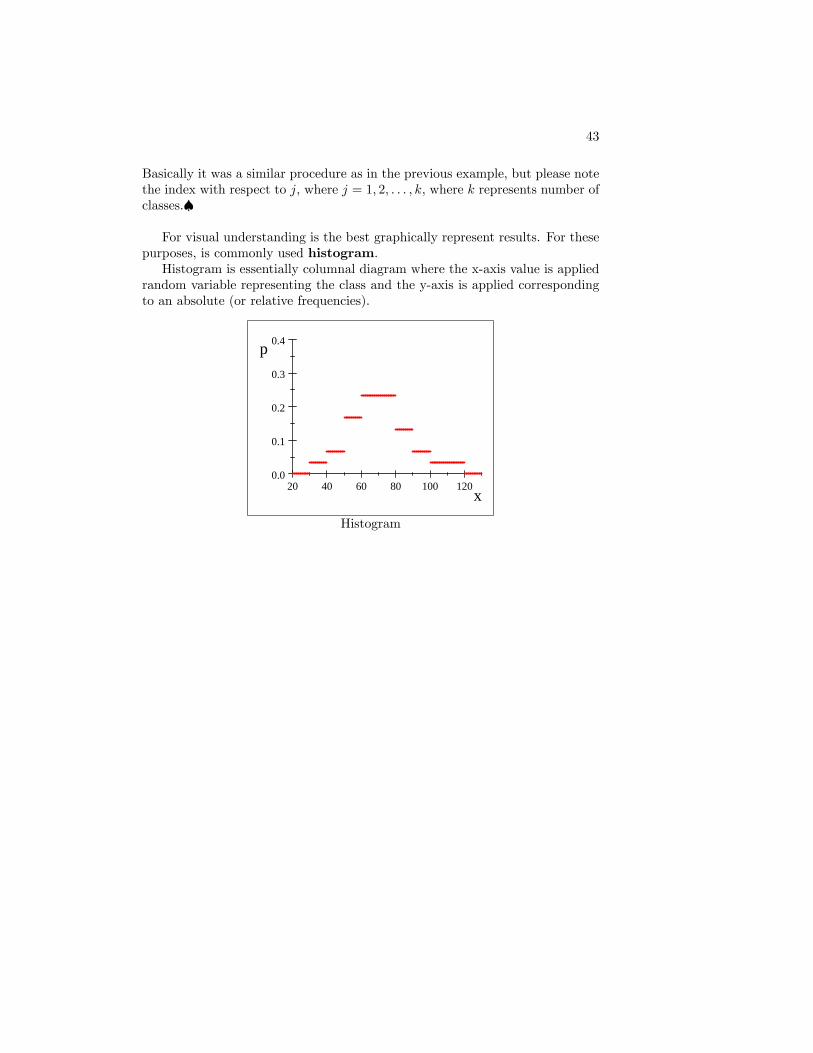
For visual understanding is the best graphically represent results. For thesepurposes, is commonly used histogram.Histogram is essentially columnal diagram where the x-axis value is applied
random variable representing the class and the y-axis is applied correspondingto an absolute (or relative frequencies).
20 40 60 80 100 1200.0
0.1
0.2
0.3
0.4
x
p
Histogram

44 CHAPTER 4. DESCRIPTIVE STATISTICS
Chapter 5
Estimates of parameters
Estimate we mean a statistical method by which the approximately determined(estimated) unknown parameters of statistical �les.Let�s random selection �1; �2; : : : ; �n of a distribution, which depends on
unknown parameters �1 , then � parameter can take only certain values ofthe area. Through the estimation theory we are trying to create statisticsT (�1; �2; : : : ; �n), which distribution comes closer to that parameter � � .Odhady, pri ktorých h
,ladáme urµcitý parameter, nazývame parametrické
odhady. Neparametrickými odhadmi nazývame odhady, pri ktorých nie je poµzadovanáparametrická �peci�kácia typu pravdepodobnostného rozdelenia.
5.1 Point estimate
Point estimate lies in replacing the unknown parameter values of the popula-tion, or its functions, the value of the selection characteristics.At some point estimate, we pay claims as to its consistency and unbias.Consistent (undisputed) point estimators � call such a set of basic statistics
Tn = T (�1; �2; : : : ; �n), that for su¢ ciently large values of index n satis�es thecondition
P (jTn ��j � ") < 1� �;
for any " > 0 and � > 0; ie.require that the parameter belongs to the interval,whose radius is less than the arbitrarily small but positive " with probability1� �; where � is any positive number, which usually is chosen close to zero aspossible. In other words, the point estimate consistent if it lie in the smallestpossible interval with most probability as can.Unbiased point estimate of the parameter� is called the basic set of statistics
Tn = T (�1; �2; : : : ; �n), which mean value holds E(Tn) = �: Otherwise, we talkabout estimating the distortion (bias). Di¤erence b (�) = E(Tn)�� we call thebias parameter estimation �. As with a growing range of n random distortion
1� is a large Greek letter "theta"
45
46 CHAPTER 5. ESTIMATES OF PARAMETERS
is reduced, then the statistics is asymptotically unbiased estimate of parameter�.
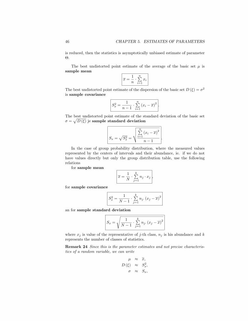
The best undistorted point estimate of the average of the basic set � issample mean
x =1
n�nPi=1
xi
The best undistorted point estimate of the dispersion of the basic set D (�) = �2
is sample covariance
S2x =1
n� 1 �nPi=1
(xi � x)2 :
The best undistorted point estimate of the standard deviation of the basic set� =
pD (�) je sample standard deviation
Sx =pS2x =
vuut nPi=1
(xi � x)2
n� 1 :
In the case of group probability distribution, where the measured valuesrepresented by the centers of intervals and their abundance, ie. if we do nothave values directly but only the group distribution table, use the followingrelationsfor sample mean
x =1
N�kPj=1
nj � xj ;
for sample covariance
S2x =1
N � 1 �kPj=1
nj� (xj � x)2
an for sample standard deviation
Sx =
s1
N � 1 �kPj=1
nj� (xj � x)2
where xj is value of the representative of j-th class, nj is his abundance and krepresents the number of classes of statistics.
Remark 24 Since this is the parameter estimates and not precise characteris-tics of a random variable, we can write
� � x;
D (�) � S2x;
� � Sx;
5.1. POINT ESTIMATE 47
but not equality.
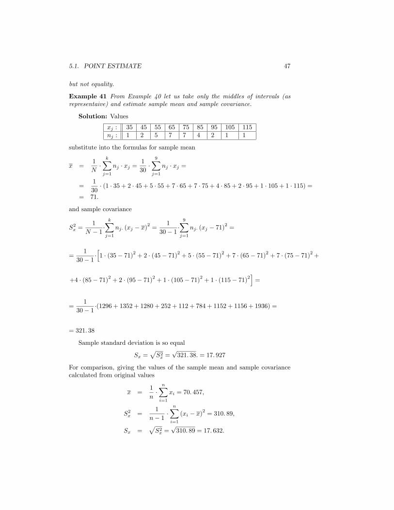
Example 41 From Example 40 let us take only the middles of intervals (asrepresentaive) and estimate sample mean and sample covariance.
Solution: Values
xj : 35 45 55 65 75 85 95 105 115nj : 1 2 5 7 7 4 2 1 1
substitute into the formulas for sample mean
x =1
N�kXj=1
nj � xj =1
30�9Xj=1
nj � xj =
=1
30� (1 � 35 + 2 � 45 + 5 � 55 + 7 � 65 + 7 � 75 + 4 � 85 + 2 � 95 + 1 � 105 + 1 � 115) =
= 71:
and sample covariance
S2x =1
N � 1 �kXj=1
nj� (xj � x)2 =1
30� 1 �9Xj=1
nj� (xj � 71)2 =
=1
30� 1 �h1 � (35� 71)2 + 2 � (45� 71)2 + 5 � (55� 71)2 + 7 � (65� 71)2 + 7 � (75� 71)2+
+4 � (85� 71)2 + 2 � (95� 71)2 + 1 � (105� 71)2 + 1 � (115� 71)2i=
=1
30� 1 �(1296 + 1352 + 1280 + 252 + 112 + 784 + 1152 + 1156 + 1936) =
= 321: 38
Sample standard deviation is so equal
Sx =pS2x =
p321: 38: = 17: 927
For comparison, giving the values of the sample mean and sample covariancecalculated from original values
x =1
n�nXi=1
xi = 70: 457;
S2x =1
n� 1 �nXi=1
(xi � x)2 = 310: 89;
Sx =pS2x =
p310: 89 = 17: 632:
48 CHAPTER 5. ESTIMATES OF PARAMETERS
We see that the values are almost identical.�
Other estimates of the mean value and median are modus.
De�nition 15 Modus is the most frequently occurring value of the characteris "most likely" value of the random variable for the character (random experi-ment)
De�nition 16 Median is represented by a value that is particularly "mean"(in this case the quotes are indeed legitimate, and really ask the reader to theconcept did not confuse with sample mean) variable in some experiment. Themedian divides the range of values for two of the almost equally likely. Forstrongly asymmetric distribution re�ects the distribution middle median betterthan mean.
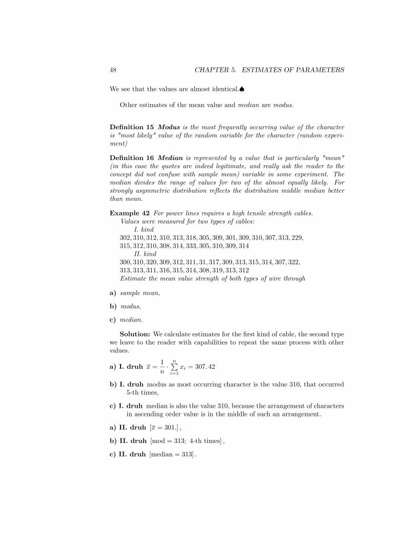
Example 42 For power lines requires a high tensile strength cables.Values were measured for two types of cables:
I. kind302; 310; 312; 310; 313; 318; 305; 309; 301; 309; 310; 307; 313; 229;315; 312; 310; 308; 314; 333; 305; 310; 309; 314
II. kind300; 310; 320; 309; 312; 311; 31; 317; 309; 313; 315; 314; 307; 322;313; 313; 311; 316; 315; 314; 308; 319; 313; 312Estimate the mean value strength of both types of wire through
a) sample mean,
b) modus,
c) median.
Solution: We calculate estimates for the �rst kind of cable, the second typewe leave to the reader with capabilities to repeat the same process with othervalues.
a) I. druh x =1
n�nPi=1
xi = 307: 42
b) I. druh modus as most occurring character is the value 310, that occurred5-th times,
c) I. druh median is also the value 310, because the arrangement of charactersin ascending order value is in the middle of such an arrangement.
a) II. druh [x = 301:] ;
b) II. druh [mod = 313; 4-th times] ;
c) II. druh [median = 313] :
5.2. INTERVAL ESTIMATION OF PARAMETERS 49
5.2 Interval estimation of parameters
In the previous section, we estimated the unknown parameter points, ie. un-known parameter was "replacing" the particular values that best estimated. Itis understandable that using a larger sample we get more accurate results thana smaller sample, but the point estimate method disregard this fact.Another possibility is to estimate the parameter interval estimation. Un-
known parameter is estimated interval, meaning that lies between two values.The center of interval is a kind estimation of parameter of mean value and
width of the interval represents the degree of dispersion of the values.This interval is called the con�dence interval (Ta; Tb) and unknown pa-
rameter � this interval will contain the probability (1 � �)%, where number� called the signi�cance level. This level is chosen in advance, and expressesthe required "degree of accuracy" with which we are looking for the interval inwhich the parameter is located.If the selection is repeated many times (given the trend of stability of sto-
chastic processes), then the unknown parameter � "falls" into the con�denceinterval (Ta; Tb) in about the 100 � (1� �)% cases (ie. the probability that theparameter is within the interval (Ta; Tb) is equal to the number 1� �).We are talking about so called 100 � (1� �)% con�dence interval and write
P (Ta � � � Tb) = 1� �
In the event that the boundaries Ta; Tb are �nite, we say about bilateral con�-dence interval.If Ta = �1, ie. (�1; Tb):::right-sided con�dence interval.If Tb =1, ie. (Ta;1):::left-sided con�dence interval.Boundaries depend on the estimated parameter, the random selection and
distribution. However, we further restrict ourselves to a normal distributionN��; �2
�, for which we estimate the parameters � and �2.
5.2.1 100 � (1 � �)% bilated con�dence interval for meanvalue �
Sample mean shoud have a normal distribution with mean E(�) = � and disper-
sion D(x) =�2
n, and so x s N
��;�2
n
�; which values we �nd by substitution
using the distribution function ��x� ���pn
�the standardized normal distri-
bution N(0; 1).For chosen � we can �nd values u(1��
2 )and �u(1��
2 ), which correspond to
the extreme values of the Gauss curve, respectively. probability that the meanvalue will be outside the chosen accuracy.With probality 1� � would be the mean value in interval
��u1��
2;u1��
2
�:
P
��u1��
2� x� �
��pn � u1��
2
�= 1� �;
50 CHAPTER 5. ESTIMATES OF PARAMETERS
� �pn� u(1��
2 )� x� � � �p
n� u(1��
2 )
�x� �pn� u1��
2� �� � �x+ �p
n� u1��
2
x� �pn� u1��
2� � � x+ �p
n� u1��
2:
So far we have assumed that we know the value of �. If we did not know herwell, we can for a su¢ ciently large statistical set (n � 30) the value of standarddeviation � point estimate with sample standard deviation Sx.In practice, however, often occur �les, whether for economic or purely prac-
tical reasons, not too large (eg when determining the quality of the productis destroyed or if it is monitoring some phenomenon of time or otherwise eco-nomically too demanding). And if the �le is small, we would be using a pointestimate committed signi�cant errors.In 1908 the English chemist Arthur Guinness Brewery & Son Brewery, W.
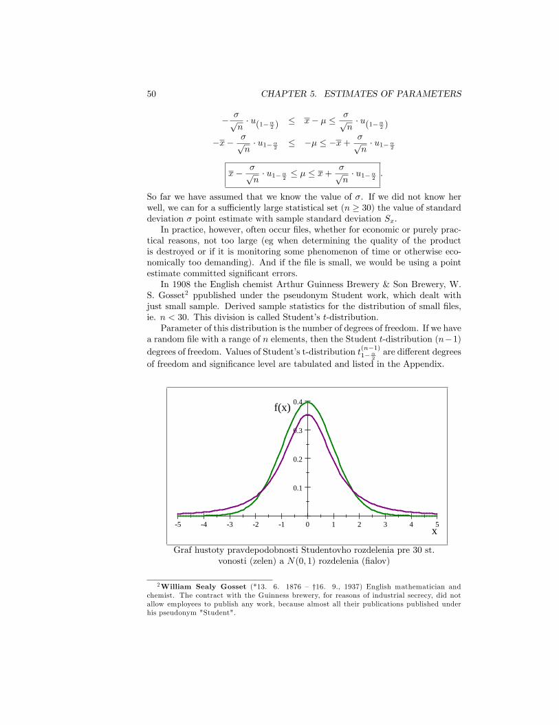
S. Gosset2 ppublished under the pseudonym Student work, which dealt withjust small sample. Derived sample statistics for the distribution of small �les,ie. n < 30. This division is called Student�s t-distribution.Parameter of this distribution is the number of degrees of freedom. If we have
a random �le with a range of n elements, then the Student t-distribution (n�1)degrees of freedom. Values of Student�s t-distribution t(n�1)1��
2are di¤erent degrees
of freedom and signi�cance level are tabulated and listed in the Appendix.
5 4 3 2 1 0 1 2 3 4 5
0.1
0.2
0.3
0.4
x
f(x)
Graf hustoty pravdepodobnosti Studentovho rozdelenia pre 30 st.vonosti (zelen) a N(0; 1) rozdelenia (�alov)
2William Sealy Gosset (*13. 6. 1876 � y16. 9., 1937) English mathematician andchemist. The contract with the Guinness brewery, for reasons of industrial secrecy, did notallow employees to publish any work, because almost all their publications published underhis pseudonym "Student".
5.2. INTERVAL ESTIMATION OF PARAMETERS 51
Graf rozdelenia pravdepodobnosti je ve,lmi podobný grafu normovaného nor-
málneho rozdelenia, av�ak krivka Studentovho rozdelenia je viac "zaoblená"okolo strednej hodnoty. Nie je ,taµzké porovnaním hustôt pravdepodobnostítýchto dvoch rozdelení dokáza ,t, µze platí:
limn!1
t(n) = N(0; 1):
So if we don´t known the value of standard deviation � we use the samplestandard deviation Sx. Sx.For large sets (n > 30) we use for con�dence interval for mean value � on
signi�cance level �; values standardized normal distribution u(1��2 ), than
x� Sxpn� u1��
2� � � x+ Sxp
n� u1��
2:
For small sets (n < 30) we use for con�dence interval for mean value � onsigni�cance level �; values Student t-distribution t(n�1)1��
2with (n� 1) degrees of
freedom, than
x� Sxpn� t(n�1)1��
2� � � x+ Sxp
n� t(n�1)1��
2:
Example 43 The airline estimates the average number of passengers. Within20 days, the average number of passengers 112 with sample variance 25.Find a 95% bilateral con�dence interval for the average number of passengers
�:
Solution: x = 112; S2x = 25 (tj.: Sx =p25 = 5); n = 20; � =
0:05:Since the �le is small (n = 20 < 30), we use Student t-distribution, where
t(20�1)1� 5%
2
= t(20�1)1� 5%
2
= t(19)1�0:025 = t
(19)0:975 = 2:1,
and the interval estimate will apply:
x� Sxpn� t(n�1)1��
2� � � x+ Sxp
n� t(n�1)1��
2;
112� 5p20� 2:1 � � � 112 + 5p
20� 2:1;
112� 2:35 � � � 112 + 2:35;109:65 � � � 114:35:�
Example 44 The automatic production lines producing rings of ball bearingssample was taken and found 50 pieces radius rings. From the measured valueswe obtain the average execution x = 70:012mm. Find a 99-percent con�denceinterval for the mean radius of the ring produced when the measured value isequal to the execution statistics S2x = 0; 00723.
52 CHAPTER 5. ESTIMATES OF PARAMETERS
Solution: x = 70:012; S2x = 0:00723 (tj.: Sx =p0:00723 = 0:08503);
n = 50; � = 0:01:
Since the �le is large (n = 50 > 30) we use standardized normal distribution,where u0:99 = 2:33, and the interval estimate will apply:
x� Sxpn� u0:995 � � � x+ Sxp
n� u0:995;
70:012� 0:08503p50
� 2:57 � � � 70:012 + 0:08503p50
� 2:57;
70:012� 0:0309 � � � 70:012 + 0:0309;69: 981 � � � 70:0429:�
Example 45 Measuring the resistance cable from eight randomly selected sam-ples obtained the following values:0:139; 0:144; 0:139; 0:140; 0:136; 0:143; 0:141; 0:136.Assume that the measured values can be considered a random realization from
a normal distribution with unknown mean and unknown variance.Find a 95% con�dence interval for the mean value.
Solution: Since we do not know the mean value E(X) or standard deviation�, we use instead samprle mean x and sample standard deviatinon Sx.
x =1
8� (0:139 + 0:144 + 0:139 + 0:140 + 0:136 + 0:143 + 0:141 + 0:136) =
= 0:13975
S2x =1
7� (0:139� 0:13975)2 + (0:144� 0:13975)2 + (0:139� 0:13975)2+
+(0:140� 0:13975)2 + (0:136� 0:13975)2 + (0:143� 0:13975)2+
+(0:141� 0:13975)2 + (0:136� 0:13975)2 = 8; 5� 10�6 = 0:0000085;
and so
Sx =pS2x =
p8; 5� 10�6 = 2:915 5� 10�3 = 0:0029155
The �le is small, therefore use the t-distribution quantiles, where t(7)0:975 = 2:365:Thus for the con�dence interval is valid:
x� Sxpn� t(7)0;975 � � � x+ Sxp
n� t(7)0;975;
0:13975� 0:0029155p8
� 2:365 � � � 0:13975 + 0:0029155p8
� 2:365;
0:13975� 2:437 8� 10�3 � � � 0:13975 + 2:437 8� 10�3;0:137 31 � � � 0:142 19:�
5.2. INTERVAL ESTIMATION OF PARAMETERS 53
5.2.2 100 � (1��)% bilateral con�dence interval for disper-sion �2
In many cases it is important to monitor not only the reliability of the averagevalue of � set, but the degree of variability �le. TThis we have in mind par-ticularly the e¤orts to reduce deviations from the average. It is clear that themanufacturer of screws with the standard 5 cm, would hardly succeed with halfof production and the other 5.5 cm 4.5 cm.To calculate the standard deviation of the con�dence interval we use more
selection division called chi-square distribution (�2).
�2-distribution3Let the random variable have n random variables x1; x2; : : : ; xn
and each has a normal distribution with mean � and standard devi-ation �. This random variables corresponding standardized randomvariables:
Z1 =x1 � ��
; : : : ; Zn =xn � ��
:
Statistics
W = Z21 + Z22 + Z
23 + : : :+ Z
2n =
nPi=1
(x1 � �)2
�2
has �2-distribution with number of degrees of freedom n.�2-distribution can also apply for distribution sampling variance
S2x: If a random selection from a fundamental set with normal dis-tribution, create the samples size n, then the random variable
�2 =(n� 1) � S2x
�2
has �2-distribution with (n� 1) degrees of freedom.
For random variabl �2 =(n� 1) � S2x
�2we can with con�dence
(1� �) determine the con�dence interval
�2�2� �2 � �21��
2;
where �2�2and �21��
2, are �
2 and�1� �
2
�quantiles �2-distribution.
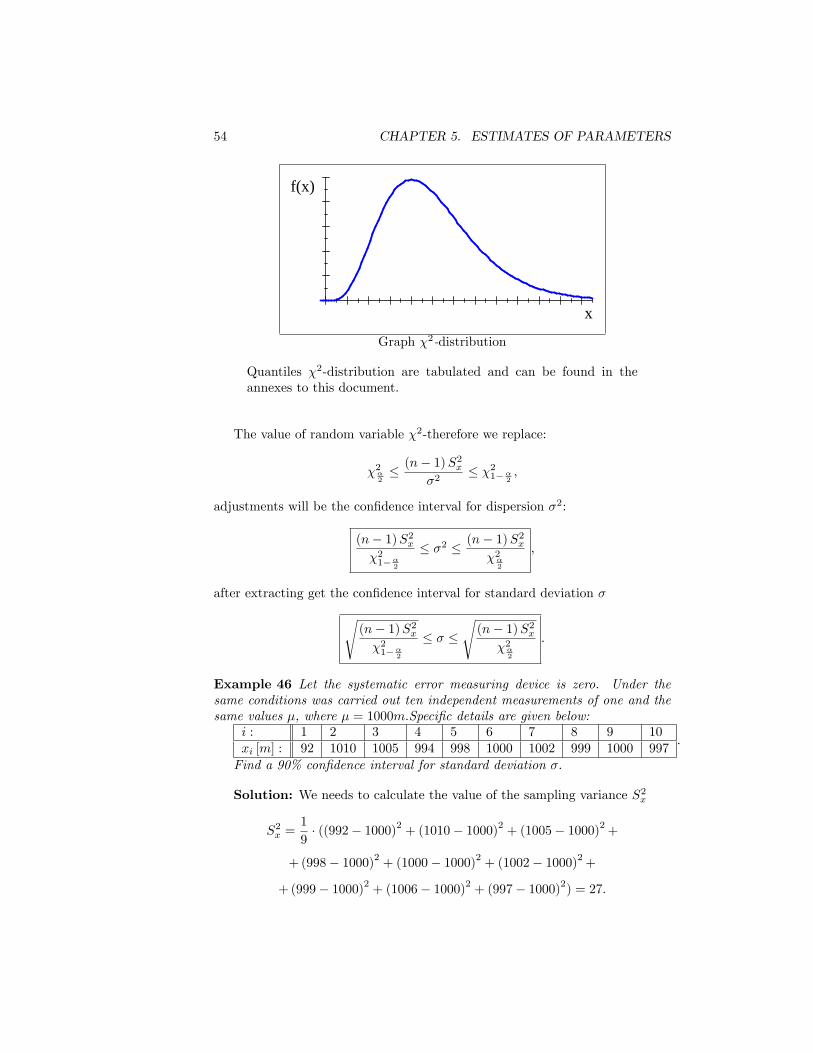
It is important to note that �2-distribution, compared to thenormal distribution is asymmetric distribution (see picture), andtherefore �2�
26= �21��
2.
3� the small Greek letter "chi"
54 CHAPTER 5. ESTIMATES OF PARAMETERS
x
f(x)
Graph �2-distribution
Quantiles �2-distribution are tabulated and can be found in theannexes to this document.
The value of random variable �2-therefore we replace:
�2�2� (n� 1)S
2x
�2� �21��
2;
adjustments will be the con�dence interval for dispersion �2:
(n� 1)S2x�21��
2
� �2 � (n� 1)S2x
�2�2
;
after extracting get the con�dence interval for standard deviation �s(n� 1)S2x�21��
2
� � �s(n� 1)S2x
�2�2
:
Example 46 Let the systematic error measuring device is zero. Under thesame conditions was carried out ten independent measurements of one and thesame values �, where � = 1000m:Speci�c details are given below:
i : 1 2 3 4 5 6 7 8 9 10xi [m] : 92 1010 1005 994 998 1000 1002 999 1000 997
:
Find a 90% con�dence interval for standard deviation �:
Solution: We needs to calculate the value of the sampling variance S2x
S2x =1
9� ((992� 1000)2 + (1010� 1000)2 + (1005� 1000)2+
+(998� 1000)2 + (1000� 1000)2 + (1002� 1000)2+
+(999� 1000)2 + (1006� 1000)2 + (997� 1000)2) = 27:
5.2. INTERVAL ESTIMATION OF PARAMETERS 55
From the tables quantiles �2-distribution we get for � = 0; 1 and n = 10,�21��
2(9) = �20;95 (9) = 16:919 a �
2�2(9) = �20;05 (9) = 3:325.
90% con�dence interval for standard deviation � iss(n� 1)S2x�21��
2
� � �s(n� 1)S2x
�2�2
;s(10� 1)S2x�20;95
� � �s(10� 1)S2x�20;05
;r9 � 2716:919
� � �r9 � 273:325
;
p14:363 � � �
p73:08;
3:789 9 � � � 8:549:�
Example 47 In laboratory experiments were needed, to maintain the standardtemperature in the laboratory 26:5 �C:In one working week was measured 46 measurements, from which the sample
average value x = 26:33 �C and sample standard deviation Sx = 0:748.Determine the 95% con�dence interval for �, �2 and �:
[(26:11; 26:55) ; (0:3; 0:62) ; (0:59; 0:79)]

56 CHAPTER 5. ESTIMATES OF PARAMETERS
Chapter 6
Testing statisticalhypotheses
The notion of statistical hypothesis understand some claim on the distributionof basic statistical �le, respectively. its parameters (for parametric tests). Veri-�cation of the veracity of such claims on the merits of random sampling is calledhypothesis testing.In its later being limited to parametric testing. We tested the parameters
mean � and variance �2 (respectively standard deviation �). Generally theparameter we denote �:
6.1 Parametric testing an single �le
Challenged the two disjoint hypotheses:null hypothesis
H0 : � = �0alternative hypothesis (the opposite claim to the null hypothesis)
H1 : � 6= �0 (bilateral test).
If we oppose unilateral test the null hypothesis is H0 : � 6= �0 and alterna-tive hypothesis:for right-side test H1 : � < �0;for left-side test H1 : � > �0:
Remark 25 For one-sided hypothesis would be more correct to formulate thenull hypothesis as H0 : � � �0 against the alternative hypothesis H1 : � < �0(respectively H0 : � � �0 against the alternative hypothesis H1 : � > �0).Below, however, dropped from the sign and also for one-sided tests the nullhypothesis we formulate H0 : � = �0.
57
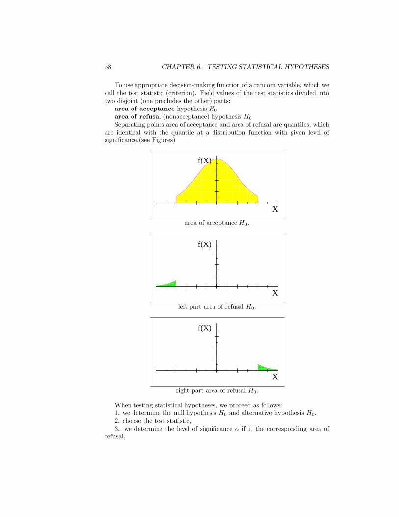
58 CHAPTER 6. TESTING STATISTICAL HYPOTHESES
To use appropriate decision-making function of a random variable, which wecall the test statistic (criterion). Field values of the test statistics divided intotwo disjoint (one precludes the other) parts:area of acceptance hypothesis H0area of refusal (nonacceptance) hypothesis H0Separating points area of acceptance and area of refusal are quantiles, which
are identical with the quantile at a distribution function with given level ofsigni�cance.(see Figures)
X
f(X)
area of acceptance H0:
X
f(X)
left part area of refusal H0:
X
f(X)
right part area of refusal H0:
When testing statistical hypotheses, we proceed as follows:1. we determine the null hypothesis H0 and alternative hypothesis H0,2. choose the test statistic,3. we determine the level of signi�cance � if it the corresponding area of
refusal,
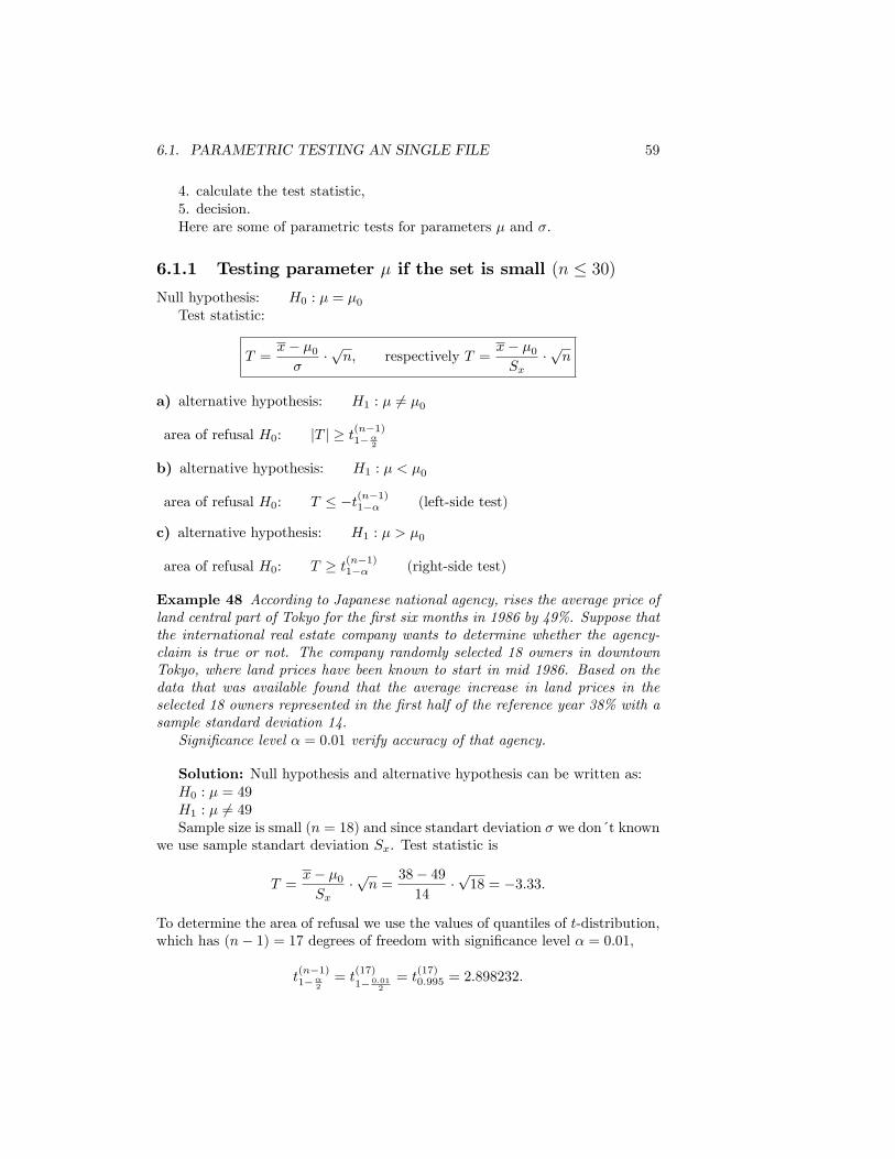
6.1. PARAMETRIC TESTING AN SINGLE FILE 59
4. calculate the test statistic,5. decision.Here are some of parametric tests for parameters � and �:
6.1.1 Testing parameter � if the set is small (n � 30)Null hypothesis: H0 : � = �0Test statistic:
T =x� �0�
�pn, respectively T =
x� �0Sx
�pn
a) alternative hypothesis: H1 : � 6= �0
area of refusal H0: jT j � t(n�1)1��2
b) alternative hypothesis: H1 : � < �0
area of refusal H0: T � �t(n�1)1�� (left-side test)
c) alternative hypothesis: H1 : � > �0
area of refusal H0: T � t(n�1)1�� (right-side test)
Example 48 According to Japanese national agency, rises the average price ofland central part of Tokyo for the �rst six months in 1986 by 49%. Suppose thatthe international real estate company wants to determine whether the agency-claim is true or not. The company randomly selected 18 owners in downtownTokyo, where land prices have been known to start in mid 1986. Based on thedata that was available found that the average increase in land prices in theselected 18 owners represented in the �rst half of the reference year 38% with asample standard deviation 14.Signi�cance level � = 0:01 verify accuracy of that agency.
Solution: Null hypothesis and alternative hypothesis can be written as:H0 : � = 49H1 : � 6= 49Sample size is small (n = 18) and since standart deviation � we don´t known
we use sample standart deviation Sx. Test statistic is
T =x� �0Sx
�pn =
38� 4914
�p18 = �3:33:
To determine the area of refusal we use the values of quantiles of t-distribution,which has (n� 1) = 17 degrees of freedom with signi�cance level � = 0:01,
t(n�1)1��
2= t
(17)
1� 0:012
= t(17)0:995 = 2:898232:
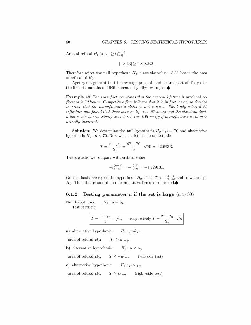
60 CHAPTER 6. TESTING STATISTICAL HYPOTHESES
Area of refusal H0 is jT j � t(n�1)1��2;
j�3:33j � 2:898232:
Therefore reject the null hypothesis H0, since the value �3:33 lies in the areaof refusal of H0.Agency�s argument that the average price of land central part of Tokyo for
the �rst six months of 1986 increased by 49%, we reject.�
Example 49 The manufacturer states that the average lifetime it produced re-�ectors is 70 hours. Competitive �rm believes that it is in fact lower, so decidedto prove that the manufacturer�s claim is not correct. Randomly selected 20re�ectors and found that their average life was 67 hours and the standard devi-ation was 5 hours. Signi�cance level � = 0:05 verify if manufacturer�s claim isactually incorrect.
Solution: We determine the null hypothesis H0 : � = 70 and alternativehypothesis H1 : � < 70: Now we calculate the test statistic
T =x� �0Sx
=67� 705
�p20 = �2:683 3:
Test statistic we compare with critical value
�t(n�1)1�� = �t(19)0;95 = �1:729131:
On this basis, we reject the hypothesis H0, since T < �t(19)0;95, and so we acceptH1. Thus the presumption of competitive �rms is con�rmed.�
6.1.2 Testing parameter � if the set is large (n > 30)
Null hypothesis: H0 : � = �0Test statistic:
T =x� �0�
�pn, respectively T =
x� �0Sx
�pn
a) alternative hypothesis: H1 : � 6= �0
area of refusal H0: jT j � u1��2
b) alternative hypothesis: H1 : � < �0
area of refusal H0: T � �u1�� (left-side test)
c) alternative hypothesis: H1 : � > �0
area of refusal H0: T � u1�� (right-side test)
6.1. PARAMETRIC TESTING AN SINGLE FILE 61
Example 50 The average time of making certain computational tasks on thecomputer is 4.56 seconds. Group of researchers tested several new algorithmsfor which assume that might increase the computing speed of the task. Thealgorithm, developed, could not say whether the average speed of implementationof tasks increased, decreased or remained unchanged. It therefore decided to testthe hypotheses that the average execution time calculation remained unchangedcompared with the scenario that the average time of calculation has changed.Conducted 200 random experiments of calculating the various tasks, which foundan average time of various tasks, which found the average time of 4.23 secondsfor their implementation (x = 4:23)and sample standard deviation 2:5 seconds(Sx = 2:5).Can we with signi�cance level � = 0:1 to conclude that the average time of
the new algorithm has been reduced?
Solution: Let́s write zero and the alternative hypothesisH0 : � = 4:56H1 : � < 4:56We use statistics
T =x� �0Sx
�pn =
4:23� 4:562:5
�p200 = �1:866 8:
The range is greater than 30, so we determine whether it falls within the �eldacceptance, which pays for
T � �u1�� = �u0:90 = �1:28:
We see that outside the �eld acceptance of hypothesis H0, therefore, must fallwithin the �eld of refusal hypothesis H0, and therefore the signi�cance level of0:1, it can be argued that the average time of the new algorithm is accelerated.�
6.1.3 Testing parameter �
Null hypothesis: H0 : � = �0Test statistics:
�2 =(n� 1)S2x
�20
a) alternative hypothesis: H1 : � 6= �0
area of refusal H0: �2 � �2�2 ;(n�1)
alebo �2 � �21��2 ;(n�1)
b) alternative hypothesis: H1 : � < �0
area of refusal H0: �2 � �2�;(n�1) (left-side test)
c) alternative hypothesis: H1 : � > �0
area of refusal H0: �2 � �21��;(n�1) (right-side test)
62 CHAPTER 6. TESTING STATISTICAL HYPOTHESES
Example 51 Standard deviation of a particular substance in tablets manufac-tured by the pharmaceutical company, shall not exceed 0.45 milligrams. If youexceed this amount, a correction must be made in setting the production line. In-spector randomly selected 25 tablets and found that the dispersion of the contentsof the substance being studied is 0.2383. What should be concluded if acknowl-edging the probality of error I. kind is 2.05 (signi�cance level � = 0:05)?
Solution: n = 25; � = 0:05; �0 = 0:45; S2x = 0:2383
H0 : � = 0:45
H1 : � > 0:45
Let́s calculate the test statistic
�2 =(n� 1)S2x
�20=(25� 1) � 0:2383
(0:45)2 = 28: 243
Quantile is �21��;(n�1) = �20:95;(24) = 36:415:
28: 243 < 36:415:
Test statistic is the acceptance area of hypothesis H0, on the signi�cance levelof 0.05 can be argued that the variability of the substance in the tablets isn´thigher than the permissible standard values, and therefore it isn´t necessary tomake correct settings of the production line.�
6.2 Comparing two �les
Often in practice we encounter a situation where we want to compare two �les.This we mean to compare these two sets of parameters, ie. whether one or moreor less than the second. or equal. We will probably compare the mean valuesof these �les, ie. parameter �1 of the �rst �le with parameter �2 of the second�le. How do we best estimates of parameter � is sample mean x.When comparing the averages of two sets we tested several hypotheses. Like
we can, whether or not equal to the averages (both-sided test), or whether oneor less. greater than the second (one-sided test). For the situations we canformulate the following hypotheses:H0 : �1 = �2againstH1 : �1 6= �2, or H1 : �1 > �2, or H1 : �1 < �2:
6.2.1 Testing equality of means of two fundamental �les,when the �les are large (n > 30), and if �1, �2 areknown
Null hypothesis:: H0 : �1 = �2
6.2. COMPARING TWO FILES 63
Test statistics:
U =(x1 � x2)s�21n1+�22n2
a) alternative hypothesis: H1 : �1 6= �2
area of refusal H0: jU j � u1��2
b) alternative hypothesis: H1 : �1 < �2
area of refusal H0: U � �u1�� (left-side test)
c) alternative hypothesis: H1 : �1 > �2
area of refusal H0: U � u1�� (right-side test)
Example 52 Site selection for new store depends on many factors. One is thelevel of household income in the area around the proposed site. Suppose that alarge store to decide whether to build its next store in town A or town B Althoughconstruction costs are lower in city B, the company decided to build in the cityand, if there are average monthly household income higher than in city B. Thesurvey of 100 randomly selected households each city found that their averagemonthly income is in A e 4380, -, in town B e 4050, -. From other sources itis known that the standard deviation of monthly household income is e 520, -at the city�s inhabitants A and e 600, - for city residents B.Can be with the signi�cance level of 5% say that the average monthly income
of households in the city and exceed the average monthly income in the householdin the city of B? Assume that income in both cities have a normal distribution.
Solution: Let́s formulate hypothesesH0 : �1 = �2H1 : �1 > �2Test statistics is
U =(x1 � x2)s�21n1+�22n2
=(4380� 4050)r5202
100+6002
100
= 4: 156 3
area of refusal H0 for � = 0:05 is U � u1�� (where u1�� = u0:95 = 0:1645) :The test statistic is found in the refusal area, so we can with signi�cance
level � = 0:05 refuse hypothesisH0 accept hypothesisH1, µzthat average monthlyincome of households in the city and are higher than in city B.�
64 CHAPTER 6. TESTING STATISTICAL HYPOTHESES
6.2.2 Testing equality of means of two fundamental �les,when the �les are small (n < 30), and if �1, �2 areknown
Null hypothesis:: H0 : �1 = �2Test statistics:
U =(x1 � x2)s�21n1+�22n2
a) alternative hypothesis: H1 : �1 6= �2
area of refusal H0: jU j � t(n1+n2�2)1��2
b) alternative hypothesis: H1 : �1 < �2
area of refusal H0: U � �t(n1+n2�2)1�� (left-side test)
c) alternative hypothesis: H1 : �1 > �2
area of refusal H0: U � t(n1+n2�2)1�� (right-side test)
6.2.3 Testing equality of means of two fundamental �les,when the �les are large (n > 30), and if �1, �2 areunknown
In the event that we do not know standard deviations �1, �2 individual �lesand these are large (n = (n1 + n2) > 30), these parameters we can replace themwith estimates Sx1 , Sx2 (sample standard deviations) and the test statistic willhave for the null hypothesis H0 : �1 = �2 form
U =(x1 � x2)sS2x1n1
+S2x2n2
For the refusal area will apply:
a) alternative hypothesis: H1 : �1 6= �2
area of refusal H0: jU j � u1��2
b) alternative hypothesis: H1 : �1 < �2
area of refusal H0: U � �u1�� (left-side test)
c) alternative hypothesis: H1 : �1 > �2
6.2. COMPARING TWO FILES 65
area of refusal H0: U � u1�� (right-side test)
Example 53 Several years ago, users of credit cards accounted for some seg-ments. Generally, people with higher incomes and spending tendency prevailedto possess an American Express card, while people with lower incomes and spend-ing more use of VISA cards. For this reason, Visa has intensi�ed its e¤orts topenetrate even more into groups with higher incomes and through ads in mag-azines and television are trying to create a greater impression on people. Aftersome time, asked the consulting company, to determine whether the averagemonthly payments through American Express Gold Card reader about equal pay-ments made Pre¤ered VISA VISA cards. The company did a survey in which1,200 randomly selected Pre¤ered Visa card holders and found that their aver-age monthly payments were $ 452 with the selection standard deviation of $ 212.Independently of this choice randomly selected 800 Gold Card holders of cards,whose average monthly payments amounted to $ 523 with the selection standarddeviation of $ 185. Holders of both cards were excluded from the survey. Surveyresults con�rmed the di¤erence between the average amount of payments madecards and VISA Gold Card Pre¤erd, overme this hypothesis signi�cance level0.01.
Solution: Let´s formulate hypothesisH0 : �1 = �2H1 : �1 6= �2Test statistics is
U =(x1 � x2)sS2x1n1
+S2x2n2
=(452� 523)r2122
1200+1852
800
= �7: 926 4
For � = 0:01 is u1��2= u0:995 = 2:58:
Area of refusal H0 is jU j � u1��2; ie. j�7: 926 4j � 2:58:We see that the test
statistic falls into it. On what basis can we claim that the average paymentsmade by the two credit cards are statistically signi�cant di¤erences.�
6.2.4 Testing equality of means of two fundamental �les,when the �les are small (n < 30), and if �1, �2 areunknown
If the standard deviation is unknown, comparing �1; �2 using independent ran-dom choices of small-scale requires in addition to the independence of choicesand normality of distribution essential �les and the additional condition thatthe variances of both random choices are equal (�1 = �2).Denote this common dispersion of both random choices �2. Its value of
course we also do not know, and therefore puts it at variance with the commonsample variance S2p of sample variances. Estimate of the variance of the popula-tion has a (n1 � 1) degrees of freedom and variance estimation of the population
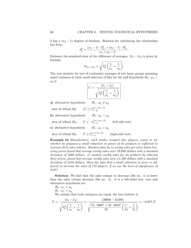
66 CHAPTER 6. TESTING STATISTICAL HYPOTHESES
2 has a (n2 � 1) degrees of freedom. Relation for calculating the relationshiphas form:
S2p =(n1 � 1) � S2x1 + (n2 � 1) � S
2x2
n1 + n2 � 2:
Estimate the standard error of the di¤erence of averages: (x1 � x2) is given byformula
S(x1�x2) =
sS2p
�1
n1+1
n2
�:
The test statistic for test of conformity averages of two basic groups assumingequal variances in their small selection of �les for the null hypothesis H0 : �1 =�2 is
U =(x1 � x2)s
S2p
�1
n1+1
n2
�a) alternative hypothesis: H1 : �1 6= �2
area of refusal H0: jU j � t(n1+n2�2)1��2
b) alternative hypothesis: H1 : �1 < �2
area of refusal H0: U � �t(n1+n2�2)1�� (left-side test)
c) alternative hypothesis: H1 : �1 > �2
area of refusal H0: U � t(n1+n2�2)1�� (right-side test)
Example 54 Manufacturer, wich mades compact disc players, wants to seewhether he proposes a small reduction in prices of its products is su¢ cient toincrease their sales volume. Random data by 14 weekly sales per store before low-ering prices found that average weekly sales were 39,600 dollars with a standarddeviation of 5060 dollars. 11 random weekly sales for its products by reducingtheir prices, found that average weekly sales were 41,200 dollars with a standarddeviation of 4010 dollars. Show the data that a small reduction in price is suf-�cient to increase the sales of CD players, if we use the level of signi�cance of0.05?
Solution: We �nd that the sales volume to decrease (�le no. 1) is lowerthan the sales volume decrease (�le no. 2). it is a left-sided test, zero andalternative hypothesis areH0 : �1 = �2H1 : �1 < �2We assume that both variances are equal, the test statistic is
U =(x1 � x2)s
S2p
�1
n1+1
n2
� = (39600� 41200)s13 � 50602 + 10 � 40102
23
�1
14+1
11
� = �0:857 17
6.2. COMPARING TWO FILES 67
The area of refusal the null hypothesis at signi�cance level � = 0:05 is
U � �t(n1+n2�2)1�� = �t(14+11�2)0:95 = �t(23)0:95 = �1:714:
Test statistic is in the area acceptance, so we with signi�cance level � = 0:05 saythat the producers proposed reducing the prices of CD players has not resultedin increase in sales volume.�

68 CHAPTER 6. TESTING STATISTICAL HYPOTHESES
Chapter 7
Correlation Analysis
Correlation, we understand each other linear relationship (dependence) of tworandom variables X and Y 1 . This relationship may be direct, ie. with increasingvalues of one variable increase in the value of the second variable and vice versa,or indirect, ie. with increasing values of one variable decreases the value of theother and vice versa.
7.1 Coe¢ cient covariance
On whether the two variables X and Y in mutual linear relationship (direct orindirect), we can see from the coe¢ cient covariance of variables X and Y (sign.:cov xy), de�nated as
cov xy =1
n�nXi=1
(xi � x) � (yi � y) = x � y � x � y :
If are variable X and Y independent, then cov xy = 0:If cov xy > 0; between X and Y exists direct linear relationship.If cov xy < 0; between X and Y existuje indirect linear relationship.
Remark 26 Covariance can be de�ned as
cov xy = E(XY )� E(X) � E(Y );
which explains the next de�nition.
Covariance of the same variable is de�ned
cov xx =1
n�nXi=1
(xi � x) � (xi � x) =1
n�nXi=1
(xi � x)2 = D(x) = �2x:
1 In this section, for clarity, dispensed with random variables by Greek letters � and insteadtags �1; �2; : : :we will use the next indication X;Y; : : :.
69
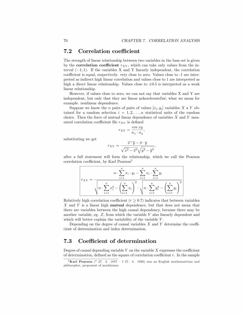
70 CHAPTER 7. CORRELATION ANALYSIS
7.2 Correlation coe¢ cient
The strength of linear relationship between two variables in the base set is givenby the correlation coe¢ cient rXY , which can take only values from the in-terval (�1; 1). If the variables X and Y linearly independent, the correlationcoe¢ cient is equal, respectively. very close to zero. Values close to -1 are inter-preted as indirect high linear correlation and values close to 1 are interpreted ashigh a direct linear relationship. Values close to �0:5 is interpreted as a weaklinear relationship.However, if values close to zero, we can not say that variables X and Y are
independent, but only that they are linear nekorelovate,lné, what we mean for
example. nonlinear dependence.Suppose we know the n pairs of pairs of values [xi; yi] variables X a Y ob-
tained for a random selection i = 1; 2; : : : ; n statistical units of the randomchoice. Then the force of mutual linear dependence of variables X and Y mea-sured correlation coe¢ cient �le rXY is de�ned
rXY =cov xy
�x � �y;
substituting we get
rXY =x � y � x � yp
x2 � x2qy2 � y2
;
after a full statement will form the relationship, which we call the Pearsoncorrelation coe¢ cient, by Karl Pearson2
rXY =
n �nXi=1
xi � yi �nXi=1
xi �nXi=1
yivuutn � nXi=1
x2i �
nXi=1
xi
!2�
vuutn � nXi=1
y2i �
nXi=1
yi
!2
Relatively high correlation coe¢ cient (r � 0:7) indicates that between variablesX and Y is a linear high mutual dependence, but that does not mean thatthere are variables between the high causal dependency, because there may beanother variable, eg. Z, from which the variable Y also linearly dependent andwhich will better explain the variability of the variable Y .Depending on the degree of causal variables X and Y determine the coe¢ -
cient of determination and index determination.
7.3 Coe¢ cient of determination
Degree of causal depending variable Y on the variableX expresses the coe¢ cientof determination, de�ned as the square of correlation coe¢ cient r. In the sample
2Karl Pearson (* 27. 3. 1857 � y 27. 4. 1936) was an English mathematician andphilosopher, proponent of machizmus.
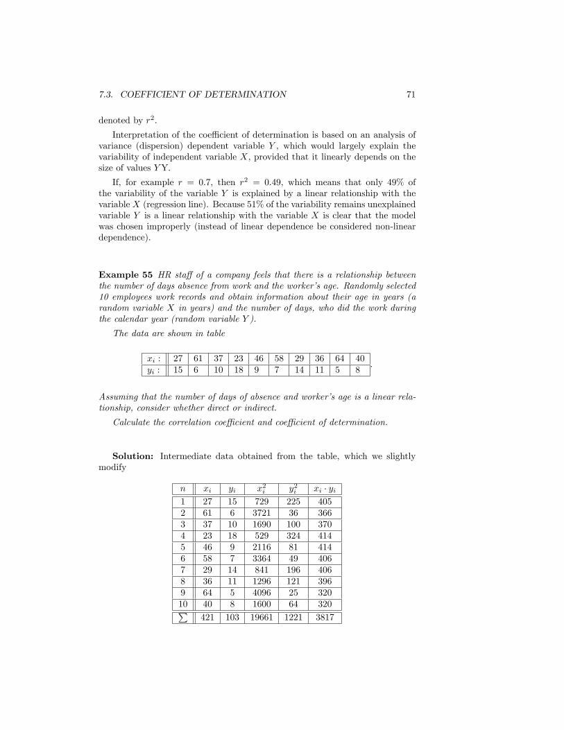
7.3. COEFFICIENT OF DETERMINATION 71
denoted by r2.
Interpretation of the coe¢ cient of determination is based on an analysis ofvariance (dispersion) dependent variable Y , which would largely explain thevariability of independent variable X, provided that it linearly depends on thesize of values YY.
If, for example r = 0:7, then r2 = 0:49, which means that only 49% ofthe variability of the variable Y is explained by a linear relationship with thevariable X (regression line). Because 51% of the variability remains unexplainedvariable Y is a linear relationship with the variable X is clear that the modelwas chosen improperly (instead of linear dependence be considered non-lineardependence).
Example 55 HR sta¤ of a company feels that there is a relationship betweenthe number of days absence from work and the worker�s age. Randomly selected10 employees work records and obtain information about their age in years (arandom variable X in years) and the number of days, who did the work duringthe calendar year (random variable Y ).
The data are shown in table
xi : 27 61 37 23 46 58 29 36 64 40yi : 15 6 10 18 9 7 14 11 5 8
:
Assuming that the number of days of absence and worker�s age is a linear rela-tionship, consider whether direct or indirect.
Calculate the correlation coe¢ cient and coe¢ cient of determination.
Solution: Intermediate data obtained from the table, which we slightlymodify
n xi yi x2i y2i xi � yi1 27 15 729 225 4052 61 6 3721 36 3663 37 10 1690 100 3704 23 18 529 324 4145 46 9 2116 81 4146 58 7 3364 49 4067 29 14 841 196 4068 36 11 1296 121 3969 64 5 4096 25 32010 40 8 1600 64 320P
421 103 19661 1221 3817
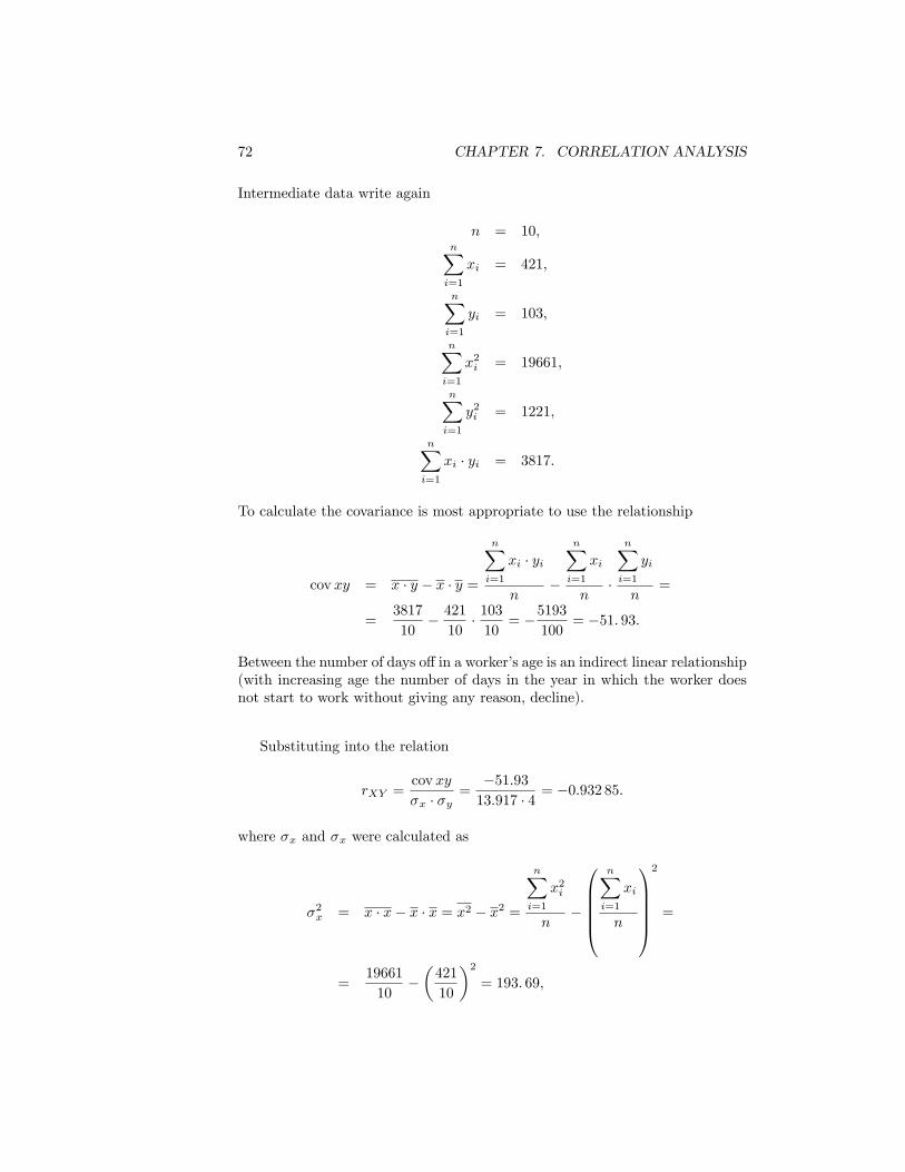
72 CHAPTER 7. CORRELATION ANALYSIS
Intermediate data write again
n = 10;nXi=1
xi = 421;
nXi=1
yi = 103;
nXi=1
x2i = 19661;
nXi=1
y2i = 1221;
nXi=1
xi � yi = 3817:
To calculate the covariance is most appropriate to use the relationship
cov xy = x � y � x � y =
nXi=1
xi � yi
n�
nXi=1
xi
n�
nXi=1
yi
n=
=3817
10� 42110� 10310
= �5193100
= �51: 93:
Between the number of days o¤ in a worker�s age is an indirect linear relationship(with increasing age the number of days in the year in which the worker doesnot start to work without giving any reason, decline).
Substituting into the relation
rXY =cov xy
�x � �y=�51:9313:917 � 4 = �0:932 85:
where �x and �x were calculated as
�2x = x � x� x � x = x2 � x2 =
nXi=1
x2i
n�
0BBBB@nXi=1
xi
n
1CCCCA2
=
=19661
10��421
10
�2= 193: 69;
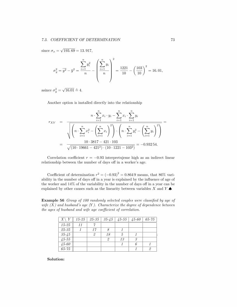
7.3. COEFFICIENT OF DETERMINATION 73
since �x =p193: 69 = 13: 917;
�2y = y2 � y2 =
nXi=1
y2i
n�
0BBBB@nXi=1
yi
n
1CCCCA2
=1221
10��103
10
�2= 16: 01;
asince �2y =p16:01 $ 4:
Another option is installed directly into the relationship
rXY =
n �nXi=1
xi � yi �nXi=1
xi �nXi=1
yivuuut0@n � nX
i=1
x2i �
nXi=1
xi
!21A �0@n � nX
i=1
y2i �
nXi=1
yi
!21A=
=10 � 3817� 421 � 103p
(10 � 19661� 4212) � (10 � 1221� 1032)= �0:932 54:
Correlation coe¢ cient r = �0:93 interpretujeme high as an indirect linearrelationship between the number of days o¤ in a worker�s age.
Coe¢ cient of determination r2 = (�0:93)2 = 0:864 9 means, that 86% vari-ability in the number of days o¤ in a year is explained by the in�uence of age ofthe worker and 14% of the variability in the number of days o¤ in a year can beexplained by other causes such as the linearity between variables X and Y .�
Example 56 Group of 100 randomly selected couples were classi�ed by age ofwife (X) and husband�s age (Y ). Characterize the degree of dependence betweenthe ages of husband and wife age coe¢ cient of correlation.
X nY 15-25 25-35 35-45 45-55 45-60 65-75
15-25 11 725-35 1 17 8 135-45 2 18 5 145-55 2 13 345-60 1 6 165-75 1 2
:
Solution:
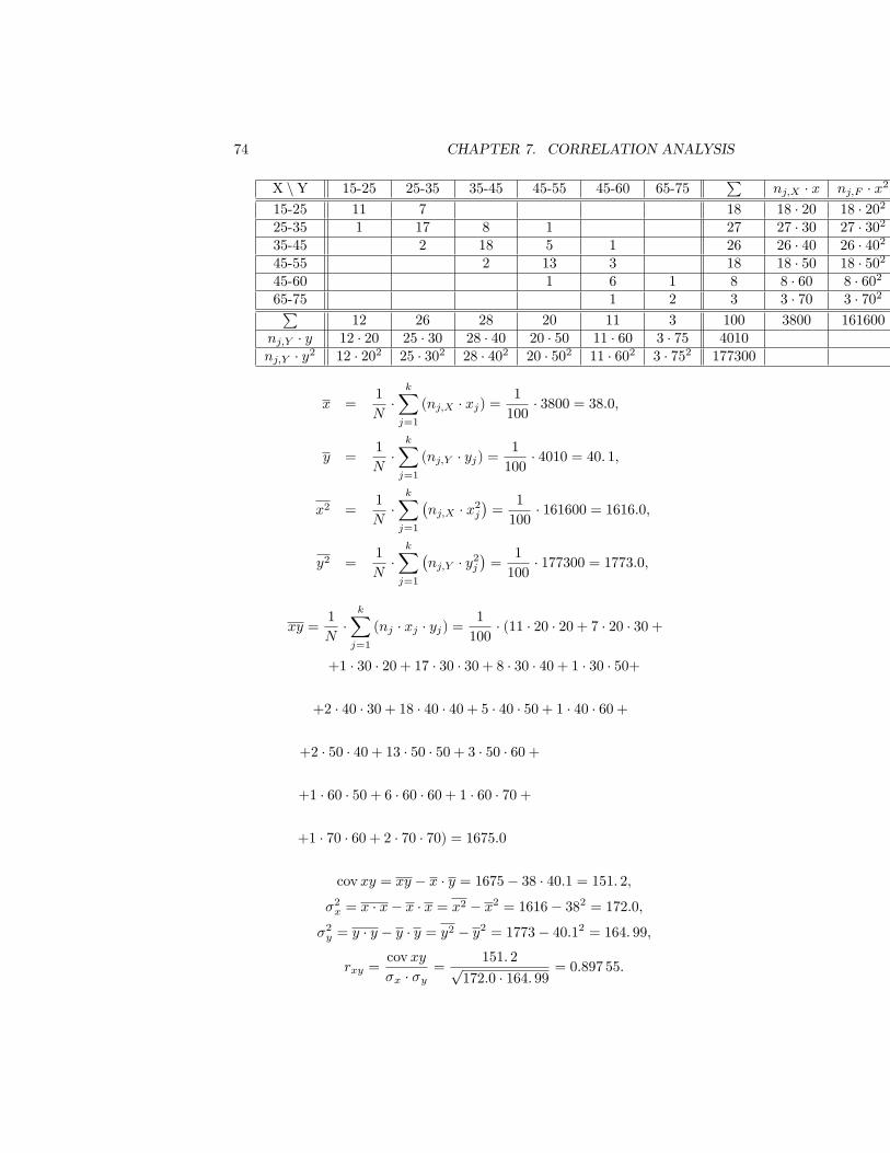
74 CHAPTER 7. CORRELATION ANALYSIS
X nY 15-25 25-35 35-45 45-55 45-60 65-75P
nj;X � x nj;F � x2
15-25 11 7 18 18 � 20 18 � 20225-35 1 17 8 1 27 27 � 30 27 � 30235-45 2 18 5 1 26 26 � 40 26 � 40245-55 2 13 3 18 18 � 50 18 � 50245-60 1 6 1 8 8 � 60 8 � 60265-75 1 2 3 3 � 70 3 � 702P
12 26 28 20 11 3 100 3800 161600nj;Y � y 12 � 20 25 � 30 28 � 40 20 � 50 11 � 60 3 � 75 4010nj;Y � y2 12 � 202 25 � 302 28 � 402 20 � 502 11 � 602 3 � 752 177300
x =1
N�kXj=1
(nj;X � xj) =1
100� 3800 = 38:0;
y =1
N�kXj=1
(nj;Y � yj) =1
100� 4010 = 40: 1;
x2 =1
N�kXj=1
�nj;X � x2j
�=
1
100� 161600 = 1616:0;
y2 =1
N�kXj=1
�nj;Y � y2j
�=
1
100� 177300 = 1773:0;
xy =1
N�kXj=1
(nj � xj � yj) =1
100� (11 � 20 � 20 + 7 � 20 � 30 +
+1 � 30 � 20 + 17 � 30 � 30 + 8 � 30 � 40 + 1 � 30 � 50+
+2 � 40 � 30 + 18 � 40 � 40 + 5 � 40 � 50 + 1 � 40 � 60 +
+2 � 50 � 40 + 13 � 50 � 50 + 3 � 50 � 60 +
+1 � 60 � 50 + 6 � 60 � 60 + 1 � 60 � 70 +
+1 � 70 � 60 + 2 � 70 � 70) = 1675:0
cov xy = xy � x � y = 1675� 38 � 40:1 = 151: 2;
�2x = x � x� x � x = x2 � x2 = 1616� 382 = 172:0;
�2y = y � y � y � y = y2 � y2 = 1773� 40:12 = 164: 99;
rxy =cov xy
�x � �y=
151: 2p172:0 � 164: 99
= 0:897 55:
7.3. COEFFICIENT OF DETERMINATION 75
Correlation coe¢ cient indicates a strong direct linear relationship between ageof wife and husband.
r2xy = 0:897 5522 = 0:805 60:
The coe¢ cient of determination, we see that 80% of the variability is explainedby the linear dependence.�
In the previous example, the value of the otherwise than we were previouslyaccustomed. Were included in the table, where each box representing a pair oftwo sets of values, devolves given abundance. In addressing the proliferation ofdeployment we properly used. Using a spreadsheet program Microsoft Excel,respectively. OpenO¢ ce Calc is also very likely to speed up routine calculations.Arranged this way data is called the correlation table.

76 CHAPTER 7. CORRELATION ANALYSIS
Chapter 8
Paired linear regression
Ak existuje medzi premennými X a Y významná lineárna závislos ,t, tj. koe-�cient korelácie je �tatisticky významný, bude nás zrejme zaujíma ,t aj rovnicapriamky, ktorá túto závislos ,t medzi premennými X a Y .reprezentuje. Urµcenieregresného modelu je dôleµzité pre urµcenie neznámej závislej premennej Y preznámu hodnotu nezávislej premennej X.Z matematiky poznáme lineárny vz ,tah ako súbor dvojíc [x; y], ktoré leµzia na
priamke Y = aX + b. V praktických situáciách, akými sa zaoberá �tatistika,vz ,tah medzi premennými X a Y nie je funkµcne lineárny, pretoµze nameranéhodnoty [xi; yi] neleµzia na priamke, ale majú tendenciu ju vytvára
,t. V takomtoprípade hovoríme o �tatistickej lineárnej závislosti.
8.1 Regression line
Suppose that we test the two physical variables X and Y , between which thereis a linear dependence
Y = a+ b �X:Parameters �0; �1 are unknown. Therefore we do an experiment in which thedetected pairs of values [x; y]. Measurement of the x values being quite right,it is often possible to set x to a predetermined level, while y is measured witherror. Therefore, a new statistical mode
yi = �0 + �1 � xi + �i; for i = 1; 2; : : : ; n;
whereyi is �{-th value variable Y in random choice,�0 � the value of Y; when variable X = 0, in random choice,�1 � regression coe¢ cient in the base set, which indicates how many
changes yi, where xi is changed by a unit of measurement,xi � �{-th value variable X in random choice,�i � random error of variable Y for �{-th observation with normal distri-
bution N�0; �2
�.
77
78 CHAPTER 8. PAIRED LINEAR REGRESSION
8.2 Estimation of the parameters �0 and �1Parameters are estimated by the method of least squares. Minimizes the sumof squares of deviations between measured and theoretical values of Y
Q (�0; �1) =nXi=1
(Yi � �0 � �1 � xi)2 ! min;
gives us system of normal equations for the regression line
�0 � n+ �1 �nXi=1
xi =nXi=1
yi;
�0 �nXi=1
xi + �1 �nXi=1
x2i =nXi=1
xi � yi:
Algebraic variety can be achieved, the coe¢ cients line �0; �1 can be calculatedalso by other relations, which are particularly useful if the unknown value [xi; yi]of sample, but we know its characteristics, such as averages of variables X andY , the standard deviation of X and Y respectively. variances, covariance ofvariables X and Y , the correlation coe¢ cient. Coe¢ cients for the regressionline then the
�1 =cov xy
�x= rXY �
r�x�y;
�0 = y � �1x:(9.1)
Example 57 Based on data from Example 55 let�s create a point estimate ofthe regression line according to the number of days of absence and age of theworker, while Let�s create a point estimate of the number of days o¤ 25-yearemployee.
Solution: From Example 55 we know that
n = 10;nXi=1
xi = 421;
nXi=1
yi = 103;
nXi=1
x2i = 19661;
nXi=1
y2i = 1221;
nXi=1
xi � yi = 3817:
8.2. ESTIMATION OF THE PARAMETERS �0 AND �1 79
Po dosadení do sústavy
�0 � n+ �1 �nXi=1
xi =nXi=1
yi;
�0 �nXi=1
xi + �1 �nXi=1
x2i =nXi=1
xi � yi;
we get
�0 � 10 + �1 � 421 = 103;
�0 � 421 + �1 � 19661 = 3817;
whose solution we get the coe¢ cients �0 = 21:587 a �1 = �0:268 and theregression equation has form
y = 21:587� 0:268 � x:
Point estimate of the number of days o¤ 25-year employee to create a simpleregression model substituting value xi = 25
yi = 21:587� 0:268 � 25 = 14: 887:
One can expect that the average number of days o¤ 25-year employee will beapproximately 15 days per calendar year.�
Example 58 Estimate the parameters of the regression line of Example 56.
Solution: Using formulas (9.1) we get
�1 =cov xy
�x=151:2
172= 0:879 07;
�0 = 40:1� 0:879 07 � 38 = 6: 695 3;
and therefore the regression line has form
y = 6: 695 3 + 0:879 07 � x:�

80 CHAPTER 8. PAIRED LINEAR REGRESSION

81
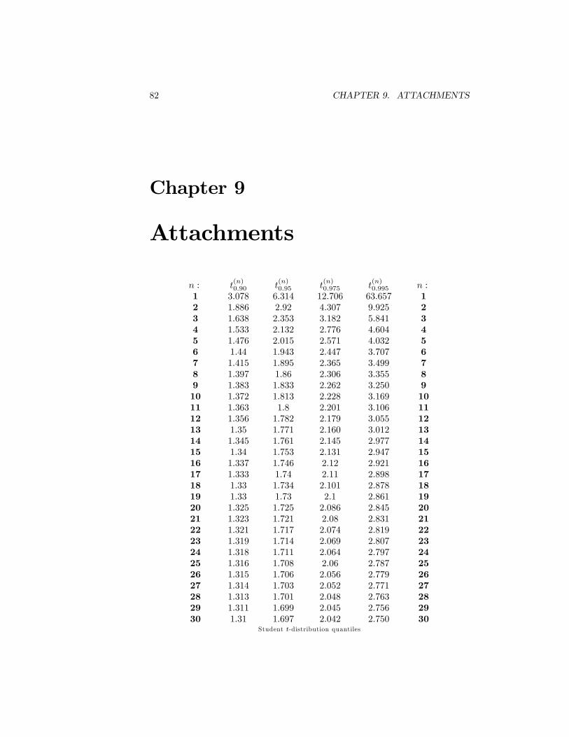
82 CHAPTER 9. ATTACHMENTS
Chapter 9
Attachments
n : t(n)0:90 t
(n)0:95 t
(n)0:975 t
(n)0:995 n :
1 3:078 6:314 12:706 63:657 12 1:886 2:92 4:307 9:925 23 1:638 2:353 3:182 5:841 34 1:533 2:132 2:776 4:604 45 1:476 2:015 2:571 4:032 56 1:44 1:943 2:447 3:707 67 1:415 1:895 2:365 3:499 78 1:397 1:86 2:306 3:355 89 1:383 1:833 2:262 3:250 910 1:372 1:813 2:228 3:169 1011 1:363 1:8 2:201 3:106 1112 1:356 1:782 2:179 3:055 1213 1:35 1:771 2:160 3:012 1314 1:345 1:761 2:145 2:977 1415 1:34 1:753 2:131 2:947 1516 1:337 1:746 2:12 2:921 1617 1:333 1:74 2:11 2:898 1718 1:33 1:734 2:101 2:878 1819 1:33 1:73 2:1 2:861 1920 1:325 1:725 2:086 2:845 2021 1:323 1:721 2:08 2:831 2122 1:321 1:717 2:074 2:819 2223 1:319 1:714 2:069 2:807 2324 1:318 1:711 2:064 2:797 2425 1:316 1:708 2:06 2:787 2526 1:315 1:706 2:056 2:779 2627 1:314 1:703 2:052 2:771 2728 1:313 1:701 2:048 2:763 2829 1:311 1:699 2:045 2:756 2930 1:31 1:697 2:042 2:750 30
Student t-distribution quantiles
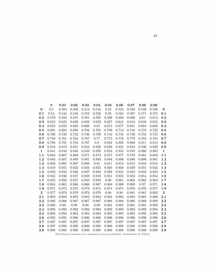
83
0 0:01 0:02 0:03 0:04 0:05 0:06 0:07 0:08 0:090 0:5 0:504 0:508 0:512 0:516 0:52 0:524 0:528 0:532 0:536 00:1 0:54 0:544 0:548 0:552 0:556 0:56 0:564 0:567 0:571 0:575 0:10:2 0:579 0:583 0:587 0:591 0:595 0:599 0:603 0:606 0:61 0:614 0:20:3 0:618 0:622 0:626 0:629 0:633 0:637 0:641 0:644 0:648 0:652 0:30:4 0:655 0:659 0:663 0:666 0:67 0:674 0:677 0:681 0:684 0:688 0:40:5 0:691 0:695 0:698 0:702 0:705 0:709 0:712 0:716 0:719 0:722 0:50:6 0:726 0:729 0:732 0:736 0:739 0:742 0:745 0:749 0:752 0:755 0:60:7 0:758 0:761 0:764 0:767 0:77 0:773 0:776 0:779 0:782 0:785 0:70:8 0:788 0:791 0:794 0:797 0:8 0:802 0:805 0:808 0:811 0:813 0:80:9 0:816 0:819 0:821 0:824 0:826 0:829 0:831 0:834 0:836 0:839 0:91 0:841 0:844 0:846 0:849 0:850 0:853 0:855 0:858 0:860 0:862 11:1 0:864 0:867 0:869 0:871 0:873 0:875 0:877 0:879 0:881 0:883 1:11:2 0:885 0:887 0:889 0:891 0:893 0:894 0:896 0:898 0:900 0:901 1:21:3 0:903 0:905 0:907 0:908 0:91 0:911 0:913 0:915 0:916 0:918 1:31:4 0:919 0:921 0:922 0:924 0:925 0:926 0:928 0:929 0:931 0:932 1:41:5 0:933 0:934 0:936 0:937 0:938 0:939 0:941 0:942 0:943 0:944 1:51:6 0:945 0:946 0:947 0:948 0:949 0:951 0:952 0:953 0:954 0:954 1:61:7 0:955 0:956 0:957 0:958 0:959 0:96 0:961 0:962 0:962 0:963 1:71:8 0:964 0:965 0:966 0:966 0:967 0:968 0:969 0:969 0:97 0:971 1:81:9 0:971 0:972 0:973 0:973 0:974 0:974 0:975 0:976 0:976 0:977 1:92 0:977 0:978 0:978 0:979 0:979 0:98 0:98 0:981 0:981 0:982 22:1 0:982 0:983 0:983 0:983 0:984 0:984 0:985 0:985 0:985 0:986 2:12:2 0:986 0:986 0:987 0:987 0:987 0:988 0:988 0:988 0:989 0:989 2:22:3 0:989 0:99 0:99 0:99 0:99 0:991 0:991 0:991 0:991 0:992 2:32:4 0:992 0:992 0:992 0:992 0:993 0:993 0:993 0:993 0:993 0:994 2:42:5 0:994 0:994 0:994 0:994 0:994 0:995 0:995 0:995 0:995 0:995 2:52:6 0:995 0:995 0:996 0:996 0:996 0:996 0:996 0:996 0:996 0:996 2:62:7 0:997 0:997 0:997 0:997 0:997 0:997 0:997 0:997 0:997 0:997 2:72:8 0:997 0:998 0:998 0:998 0:998 0:998 0:998 0:998 0:998 0:998 2:82:9 0:998 0:998 0:998 0:998 0:998 0:998 0:998 0:999 0:999 0:999 2:9
Distribution function of a standard normal probability distribution �sN(0;1)
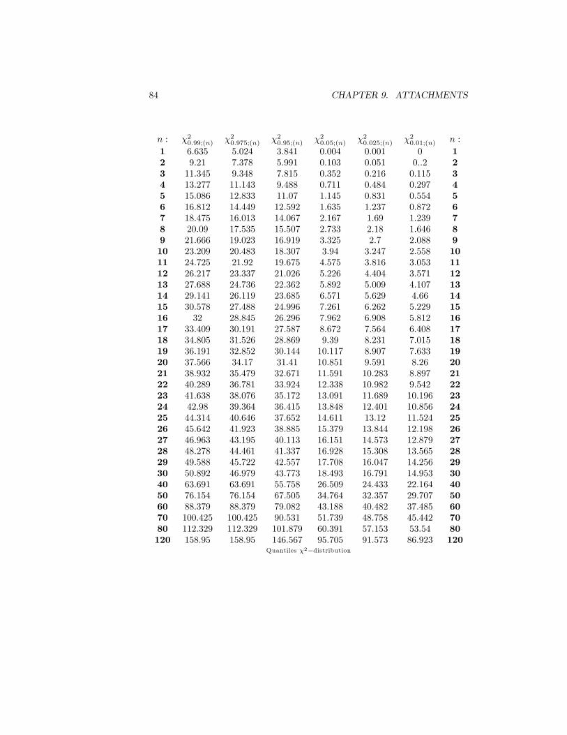
84 CHAPTER 9. ATTACHMENTS
n : �20:99;(n) �20:975;(n) �20:95;(n) �20:05;(n) �20:025;(n) �20:01;(n) n :
1 6:635 5:024 3:841 0:004 0:001 0 12 9:21 7:378 5:991 0:103 0:051 0::2 23 11:345 9:348 7:815 0:352 0:216 0:115 34 13:277 11:143 9:488 0:711 0:484 0:297 45 15:086 12:833 11:07 1:145 0:831 0:554 56 16:812 14:449 12:592 1:635 1:237 0:872 67 18:475 16:013 14:067 2:167 1:69 1:239 78 20:09 17:535 15:507 2:733 2:18 1:646 89 21:666 19:023 16:919 3:325 2:7 2:088 910 23:209 20:483 18:307 3:94 3:247 2:558 1011 24:725 21:92 19:675 4:575 3:816 3:053 1112 26:217 23:337 21:026 5:226 4:404 3:571 1213 27:688 24:736 22:362 5:892 5:009 4:107 1314 29:141 26:119 23:685 6:571 5:629 4:66 1415 30:578 27:488 24:996 7:261 6:262 5:229 1516 32 28:845 26:296 7:962 6:908 5:812 1617 33:409 30:191 27:587 8:672 7:564 6:408 1718 34:805 31:526 28:869 9:39 8:231 7:015 1819 36:191 32:852 30:144 10:117 8:907 7:633 1920 37:566 34:17 31:41 10:851 9:591 8:26 2021 38:932 35:479 32:671 11:591 10:283 8:897 2122 40:289 36:781 33:924 12:338 10:982 9:542 2223 41:638 38:076 35:172 13:091 11:689 10:196 2324 42:98 39:364 36:415 13:848 12:401 10:856 2425 44:314 40:646 37:652 14:611 13:12 11:524 2526 45:642 41:923 38:885 15:379 13:844 12:198 2627 46:963 43:195 40:113 16:151 14:573 12:879 2728 48:278 44:461 41:337 16:928 15:308 13:565 2829 49:588 45:722 42:557 17:708 16:047 14:256 2930 50:892 46:979 43:773 18:493 16:791 14:953 3040 63:691 63:691 55:758 26:509 24:433 22:164 4050 76:154 76:154 67:505 34:764 32:357 29:707 5060 88:379 88:379 79:082 43:188 40:482 37:485 6070 100:425 100:425 90:531 51:739 48:758 45:442 7080 112:329 112:329 101:879 60:391 57:153 53:54 80120 158:95 158:95 146:567 95:705 91:573 86:923 120
Quantiles �2�distribution

Bibliography
[1] J. Chajdiak, E. Rublíková, M. Gudába - �TATISTICKÉ METÓDY VPRAXI, STATIS Bratislava 1994.
85