Fundamentals of Mathematical Statistics - …gilvanguedes.com/wp-content/uploads/2018/03/... ·...

674

C-1 Populations, Parameters, and Random SamplingStatistical inference involves learning something about a population given the availability of a sam-ple from that population. By population, we mean any well-defined group of subjects, which could be individuals, firms, cities, or many other possibilities. By “learning,” we can mean several things, which are broadly divided into the categories of estimation and hypothesis testing.

A couple of examples may help you understand these terms. In the population of all working adults in the United States, labor economists are interested in learning about the return to education, as measured by the average percentage increase in earnings given another year of education. It would be impractical and costly to obtain information on earnings and education for the entire working population in the United States, but we can obtain data on a subset of the population. Using the data collected, a labor economist may report that his or her best estimate of the return to another year of education is 7.5%. This is an example of a point estimate. Or, she or he may report a range, such as “the return to education is between 5.6% and 9.4%.” This is an example of an interval estimate.

An urban economist might want to know whether neighborhood crime watch programs are associ-ated with lower crime rates. After comparing crime rates of neighborhoods with and without such pro-grams in a sample from the population, he or she can draw one of two conclusions: neighborhood watch programs do affect crime, or they do not. This example falls under the rubric of hypothesis testing.

The first step in statistical inference is to identify the population of interest. This may seem obvi-ous, but it is important to be very specific. Once we have identified the population, we can specify a model for the population relationship of interest. Such models involve probability distributions or features of probability distributions, and these depend on unknown parameters. Parameters are simply constants that determine the directions and strengths of relationships among variables. In the labor eco-nomics example just presented, the parameter of interest is the return to education in the population.

C-1a SamplingFor reviewing statistical inference, we focus on the simplest possible setting. Let Y be a random variable representing a population with a probability density function f 1y; u 2 , which depends on the single parameter u. The probability density function (pdf) of Y is assumed to be known except for the value of u; different values of u imply different population distributions, and therefore we are interested in the value of u. If we can obtain certain kinds of samples from the population, then we can learn something about u. The easiest sampling scheme to deal with is random sampling.

Fundamentals of Mathematical Statistics

Appendix C

Copyright 2016 Cengage Learning. All Rights Reserved. May not be copied, scanned, or duplicated, in whole or in part. Due to electronic rights, some third party content may be suppressed from the eBook and/or eChapter(s).

Editorial review has deemed that any suppressed content does not materially affect the overall learning experience. Cengage Learning reserves the right to remove additional content at any time if subsequent rights restrictions require it.

Appendix C Fundamentals of Mathematical Statistics 675

Random Sampling. If Y1, Y2, p , Yn are independent random variables with a common prob-ability density function f 1y; u 2 , then 5Y1, p , Yn6 is said to be a random sample from f 1y; u 2 [or a random sample from the population represented by f 1y; u 2 ].

When 5Y1, p , Yn6 is a random sample from the density f 1y; u 2 , we also say that the Yi are indepen-dent, identically distributed (or i.i.d.) random variables from f 1y; u 2 . In some cases, we will not need to entirely specify what the common distribution is.

The random nature of Y1, Y2, p , Yn in the definition of random sampling reflects the fact that many different outcomes are possible before the sampling is actually carried out. For example, if fam-ily income is obtained for a sample of n 5 100 families in the United States, the incomes we observe will usually differ for each different sample of 100 families. Once a sample is obtained, we have a set of numbers, say, 5y1, y2, p , yn6, which constitute the data that we work with. Whether or not it is ap-propriate to assume the sample came from a random sampling scheme requires knowledge about the actual sampling process.

Random samples from a Bernoulli distribution are often used to illustrate statistical concepts, and they also arise in empirical applications. If Y1, Y2, p , Yn are independent random variables and each is distributed as Bernoulli(u), so that P 1Yi 5 1 2 5 u and P 1Yi 5 0 2 5 1 2 u, then 5Y1, Y2, p , Yn6 constitutes a random sample from the Bernoulli(u) distribution. As an illustration, consider the airline reservation example carried along in Appendix B. Each Yi denotes whether customer i shows up for his or her reservation; Yi 5 1 if passenger i shows up, and Yi 5 0 otherwise. Here, u is the probability that a randomly drawn person from the population of all people who make airline reservations shows up for his or her reservation.

For many other applications, random samples can be assumed to be drawn from a normal distri-bution. If 5Y1, p , Yn6 is a random sample from the Normal 1m, s2 2 population, then the population is characterized by two parameters, the mean m and the variance s2. Primary interest usually lies in m, but s2 is of interest in its own right because making inferences about m often requires learning about s2.

C-2 Finite Sample Properties of EstimatorsIn this section, we study what are called finite sample properties of estimators. The term “finite sample” comes from the fact that the properties hold for a sample of any size, no matter how large or small. Sometimes, these are called small sample properties. In Section C-3, we cover “asymptotic properties,” which have to do with the behavior of estimators as the sample size grows without bound.

C-2a Estimators and EstimatesTo study properties of estimators, we must define what we mean by an estimator. Given a random sam-ple 5Y1, Y2, p , Yn6 drawn from a population distribution that depends on an unknown parameter u, an estimator of u is a rule that assigns each possible outcome of the sample a value of u. The rule is specified before any sampling is carried out; in particular, the rule is the same regardless of the data actually obtained.

As an example of an estimator, let 5Y1, p , Yn6 be a random sample from a population with mean m. A natural estimator of m is the average of the random sample:

Y 5 n21 ani51

Yi. [C.1]

Y is called the sample average but, unlike in Appendix A where we defined the sample average of a set of numbers as a descriptive statistic, Y is now viewed as an estimator. Given any outcome of the random variables Y1, p , Yn, we use the same rule to estimate m: we simply average them. For actual data outcomes 5y1, p , yn6, the estimate is just the average in the sample: y 5 1y1 1 y2 1 p 1 yn 2 /n.



Appendices676

ExamplE C.1 City Unemployment Rates

Suppose we obtain the following sample of unemployment rates for 10 cities in the United States:

City Unemployment Rate

1 5.1

2 6.4

3 9.2

4 4.1

5 7.5

6 8.3

7 2.6

8 3.5

9 5.8

10 7.5

Our estimate of the average city unemployment rate in the United States is y 5 6.0. Each sample gen-erally results in a different estimate. But the rule for obtaining the estimate is the same, regardless of which cities appear in the sample, or how many.

More generally, an estimator W of a parameter u can be expressed as an abstract mathematical formula:

W 5 h 1Y1, Y2, p Yn 2 , [C.2]

for some known function h of the random variables Y1, Y2, p , Yn. As with the special case of the sample average, W is a random variable because it depends on the random sample: as we obtain different random samples from the population, the value of W can change. When a particular set of numbers, say, 5y1, y2, p , yn6, is plugged into the function h, we obtain an estimate of u, denoted w 5 h 1y1, p , yn 2 . Sometimes, W is called a point estimator and w a point estimate to distinguish these from interval estimators and estimates, which we will come to in Section C-5.

For evaluating estimation procedures, we study various properties of the probability distribution of the random variable W. The distribution of an estimator is often called its sampling distribution, because this distribution describes the likelihood of various outcomes of W across different random samples. Because there are unlimited rules for combining data to estimate parameters, we need some sensible criteria for choosing among estimators, or at least for eliminating some estimators from con-sideration. Therefore, we must leave the realm of descriptive statistics, where we compute things such as the sample average to simply summarize a body of data. In mathematical statistics, we study the sampling distributions of estimators.

C-2b UnbiasednessIn principle, the entire sampling distribution of W can be obtained given the probability distribution of Yi and the function h. It is usually easier to focus on a few features of the distribution of W in evaluating it as an estimator of u. The first important property of an estimator involves its expected value.

Unbiased Estimator. An estimator, W of u, is an unbiased estimator if

E 1W 2 5 u, [C.3]

for all possible values of u.




If an estimator is unbiased, then its probability distribution has an expected value equal to the parameter it is supposed to be estimating. Unbiasedness does not mean that the estimate we get with any particular sample is equal to u, or even very close to u. Rather, if we could indefinitely draw random samples on Y from the population, compute an estimate each time, and then average these estimates over all random samples, we would obtain u. This thought experiment is abstract because, in most applications, we just have one random sample to work with.

For an estimator that is not unbiased, we define its bias as follows.

Bias of an Estimator. If W is a biased estimator of u, its bias is defined

Bias 1W 2 ; E 1W 2 2 u. [C.4]

Figure C.1 shows two estimators; the first one is unbiased, and the second one has a positive bias.The unbiasedness of an estimator and the size of any possible bias depend on the distribution of Y

and on the function h. The distribution of Y is usually beyond our control (although we often choose a model for this distribution): it may be determined by nature or social forces. But the choice of the rule h is ours, and if we want an unbiased estimator, then we must choose h accordingly.

Some estimators can be shown to be unbiased quite generally. We now show that the sample average Y is an unbiased estimator of the population mean m, regardless of the underlying population distribution. We use the properties of expected values (E.1 and E.2) that we covered in Section B-3:

E 1Y 2 5 Ea 11/n 2 ani51

Yib 5 11/n 2Eaani51

Yib 5 11/n 2 aani51

E 1Yi 2 b

5 11/n 2 aani51

mb 5 11/n 2 1nm 2 5 m.

wu = E(W1) E(W2)

pdf of W1 pdf of W2

f(w)

Figure C.1 An unbiased estimator, W1, and an estimator with positive bias, W2.



Appendices678

For hypothesis testing, we will need to estimate the variance s2 from a population with mean m. Letting 5Y1, p , Yn6 denote the random sample from the population with E 1Y 2 5 m and Var 1Y 2 5 s2, define the estimator as

S2 51

n 2 1 ani51

1Yi 2 Y 2 2, [C.5]

which is usually called the sample variance. It can be shown that S2 is unbiased for s2: E 1S2 2 5 s2. The division by n 2 1, rather than n, accounts for the fact that the mean m is estimated rather than known. If m were known, an unbiased estimator of s2 would be n21g n

i51 1Yi 2 m 2 2, but m is rarely known in practice.

Although unbiasedness has a certain appeal as a property for an estimator—indeed, its antonym, “biased,” has decidedly negative connotations—it is not without its problems. One weakness of unbi-asedness is that some reasonable, and even some very good, estimators are not unbiased. We will see an example shortly.

Another important weakness of unbiasedness is that unbiased estimators exist that are actually quite poor estimators. Consider estimating the mean m from a population. Rather than using the sample average Y to estimate m, suppose that, after collecting a sample of size n, we discard all of the observa-tions except the first. That is, our estimator of m is simply W ; Y1. This estimator is unbiased because E 1Y1 2 5 m. Hopefully, you sense that ignoring all but the first observation is not a prudent approach to estimation: it throws out most of the information in the sample. For example, with n 5 100, we obtain 100 outcomes of the random variable Y, but then we use only the first of these to estimate E(Y).

C-2d The Sampling Variance of Estimators

The example at the end of the previous subsection shows that we need additional criteria to evaluate estimators. Unbiasedness only ensures that the sampling distribution of an estimator has a mean value equal to the parameter it is supposed to be estimating. This is fine, but we also need to know how spread out the distribution of an estimator is. An estimator can be equal to u, on average, but it can also be very far away with large probability. In Figure C.2, W1 and W2 are both unbiased estimators of u. But the distribution of W1 is more tightly centered about u: the probability that W1 is greater than any given distance from u is less than the probability that W2 is greater than that same distance from u. Using W1 as our estimator means that it is less likely that we will obtain a random sample that yields an estimate very far from u.

To summarize the situation shown in Figure C.2, we rely on the variance (or standard deviation) of an estimator. Recall that this gives a single measure of the dispersion in the distribution. The vari-ance of an estimator is often called its sampling variance because it is the variance associated with a sampling distribution. Remember, the sampling variance is not a random variable; it is a constant, but it might be unknown.

We now obtain the variance of the sample average for estimating the mean m from a population:

Var 1Y 2 5 Vara 11/n 2 ani51

Yib 5 11/n2 2Varaani51

Yib 5 11/n2 2 aani51

Var 1Yi 2 b

5 11/n2 2 aani51

s2b 5 11/n2 2 1ns2 2 5 s2/n. [C.6]

Notice how we used the properties of variance from Sections B-3 and B-4 (VAR.2 and VAR.4), as well as the independence of the Yi. To summarize: If 5Yi: i 5 1, 2, p , n6 is a random sample from a population with mean m and variance s2, then Y has the same mean as the population, but its sampling variance equals the population variance, s2, divided by the sample size.




An important implication of Var 1Y 2 5 s2/n is that it can be made very close to zero by increasing the sample size n. This is a key feature of a reasonable estimator, and we return to it in Section C-3.

As suggested by Figure C.2, among unbiased estimators, we prefer the estimator with the small-est variance. This allows us to eliminate certain estimators from consideration. For a random sample from a population with mean m and variance s2, we know that Y is unbiased and Var 1Y 2 5 s2/n. What about the estimator Y1, which is just the first observation drawn? Because Y1 is a random draw from the population, Var 1Y1 2 5 s2. Thus, the difference between Var 1Y1 2 and Var 1Y 2 can be large even for small sample sizes. If n 5 10, then Var 1Y1 2 is 10 times as large as Var 1Y 2 5 s2/10. This gives us a formal way of excluding Y1 as an estimator of m.

To emphasize this point, Table C.1 contains the outcome of a small simulation study. Using the statistical package Stata®, 20 random samples of size 10 were generated from a normal distribution, with m 5 2 and s2 5 1; we are interested in estimating m here. For each of the 20 random samples, we compute two estimates, y1 and y; these values are listed in Table C.1. As can be seen from the table, the values for y1 are much more spread out than those for y: y1 ranges from 20.64 to 4.27, while y ranges only from 1.16 to 2.58. Further, in 16 out of 20 cases, y is closer than y1 to m 5 2. The aver-age of y1 across the simulations is about 1.89, while that for y is 1.96. The fact that these averages are close to 2 illustrates the unbiasedness of both estimators (and we could get these averages closer to 2 by doing more than 20 replications). But comparing just the average outcomes across random draws masks the fact that the sample average Y is far superior to Y1 as an estimator of m.

C-2e Efficiency

Comparing the variances of Y and Y1 in the previous subsection is an example of a general approach to comparing different unbiased estimators.

Relative Efficiency. If W1 and W2 are two unbiased estimators of u, W1 is efficient relative to W2 when Var 1W1 2 # Var 1W2 2 for all u, with strict inequality for at least one value of u.

wu

f(w)

pdf of W1

pdf of W2

Figure C.2 The sampling distributions of two unbiased estimators of u.



Appendices680

TAble C.1 Simulation of Estimators for a Normal 1m, 12 Distribution with m 5 2Replication y1 y

1 20.64 1.98

2 1.06 1.43

3 4.27 1.65

4 1.03 1.88

5 3.16 2.34

6 2.77 2.58

7 1.68 1.58

8 2.98 2.23

9 2.25 1.96

10 2.04 2.11

11 0.95 2.15

12 1.36 1.93

13 2.62 2.02

14 2.97 2.10

15 1.93 2.18

16 1.14 2.10

17 2.08 1.94

18 1.52 2.21

19 1.33 1.16

20 1.21 1.75

Earlier, we showed that, for estimating the population mean m, Var 1Y 2 , Var 1Y1 2 for any value of s2 whenever n . 1. Thus, Y is efficient relative to Y1 for estimating m. We cannot always choose between unbiased estimators based on the smallest variance criterion: given two unbiased estimators of u, one can have smaller variance from some values of u, while the other can have smaller variance for other values of u.

If we restrict our attention to a certain class of estimators, we can show that the sample average has the smallest variance. Problem C.2 asks you to show that Y has the smallest variance among all unbiased estimators that are also linear functions of Y1, Y2, p , Yn. The assumptions are that the Yi have common mean and variance, and that they are pairwise uncorrelated.

If we do not restrict our attention to unbiased estimators, then comparing variances is meaning-less. For example, when estimating the population mean m, we can use a trivial estimator that is equal to zero, regardless of the sample that we draw. Naturally, the variance of this estimator is zero (since it is the same value for every random sample). But the bias of this estimator is 2m, so it is a very poor estimator when 0m 0 is large.

One way to compare estimators that are not necessarily unbiased is to compute the mean squared error (MSE) of the estimators. If W is an estimator of u, then the MSE of W is defined as MSE 1W 2 5 E 3 1W 2 u 2 2 4. The MSE measures how far, on average, the estimator is away from u. It can be shown that MSE 1W 2 5 Var 1W 2 1 3Bias 1W 2 42, so that MSE(W) depends on the variance and bias (if any is present). This allows us to compare two estimators when one or both are biased.




C-3 Asymptotic or Large Sample Properties of EstimatorsIn Section C-2, we encountered the estimator Y1 for the population mean m, and we saw that, even though it is unbiased, it is a poor estimator because its variance can be much larger than that of the sample mean. One notable feature of Y1 is that it has the same variance for any sample size. It seems reasonable to require any estimation procedure to improve as the sample size increases. For estimat-ing a population mean m, Y improves in the sense that its variance gets smaller as n gets larger; Y1 does not improve in this sense.

We can rule out certain silly estimators by studying the asymptotic or large sample properties of estimators. In addition, we can say something positive about estimators that are not unbiased and whose variances are not easily found.

Asymptotic analysis involves approximating the features of the sampling distribution of an es-timator. These approximations depend on the size of the sample. Unfortunately, we are necessarily limited in what we can say about how “large” a sample size is needed for asymptotic analysis to be appropriate; this depends on the underlying population distribution. But large sample approximations have been known to work well for sample sizes as small as n 5 20.

C-3a ConsistencyThe first asymptotic property of estimators concerns how far the estimator is likely to be from the parameter it is supposed to be estimating as we let the sample size increase indefinitely.

Consistency. Let Wn be an estimator of u based on a sample Y1, Y2, p , Yn of size n. Then, Wn is a consistent estimator of u if for every e . 0,

P 1 0Wn 2 u 0 . e 2 S 0 as n S `. [C.7]

If Wn is not consistent for u, then we say it is inconsistent.When Wn is consistent, we also say that u is the probability limit of Wn, written

as plim 1Wn 2 5 u.Unlike unbiasedness—which is a feature of an estimator for a given sample size—consistency

involves the behavior of the sampling distribution of the estimator as the sample size n gets large. To emphasize this, we have indexed the estimator by the sample size in stating this definition, and we will continue with this convention throughout this section.

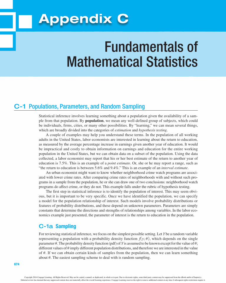
Equation (C.7) looks technical, and it can be rather difficult to establish based on fundamental probability principles. By contrast, interpreting (C.7) is straightforward. It means that the distribution of Wn becomes more and more concentrated about u, which roughly means that for larger sample sizes, Wn is less and less likely to be very far from u. This tendency is illustrated in Figure C.3.

If an estimator is not consistent, then it does not help us to learn about u, even with an unlimited amount of data. For this reason, consistency is a minimal requirement of an estimator used in statis-tics or econometrics. We will encounter estimators that are consistent under certain assumptions and inconsistent when those assumptions fail. When estimators are inconsistent, we can usually find their probability limits, and it will be important to know how far these probability limits are from u.

As we noted earlier, unbiased estimators are not necessarily consistent, but those whose vari-ances shrink to zero as the sample size grows are consistent. This can be stated formally: If Wn is an unbiased estimator of u and Var 1Wn 2 S 0 as n S `, then plim 1Wn 2 5 u. Unbiased estimators that use the entire data sample will usually have a variance that shrinks to zero as the sample size grows, thereby being consistent.

A good example of a consistent estimator is the average of a random sample drawn from a popu-lation with mean m and variance s2. We have already shown that the sample average is unbiased for m.



Appendices682

In Equation (C.6), we derived Var 1Yn 2 5 s2/n for any sample size n. Therefore, Var 1Yn 2 S 0 as n S `, so Yn is a consistent estimator of m (in addition to being unbiased).

The conclusion that Yn is consistent for m holds even if Var 1Yn 2 does not exist. This classic result is known as the law of large numbers (LLN).

Law of Large Numbers. Let Y1, Y2, p , Yn be independent, identically distributed random variables with mean m. Then,

plim 1Yn 2 5 m. [C.8]

The law of large numbers means that, if we are interested in estimating the population average m, we can get arbitrarily close to m by choosing a sufficiently large sample. This fundamental result can be combined with basic properties of plims to show that fairly complicated estimators are consistent.

Property PLim.1: Let u be a parameter and define a new parameter, g 5 g 1u 2 , for some continuous function g 1u 2 . Suppose that plim 1Wn 2 5 u. Define an estimator of g by Gn 5 g 1Wn 2 . Then,

plim 1Gn 2 5 g. [C.9]

This is often stated as

plim g 1Wn 2 5 g 1plim Wn 2 [C.10]

for a continuous function g 1u 2 .The assumption that g 1u 2 is continuous is a technical requirement that has often been described

nontechnically as “a function that can be graphed without lifting your pencil from the paper.” Because all the functions we encounter in this text are continuous, we do not provide a formal definition of a continuous function. Examples of continuous functions are g 1u 2 5 a 1 bu for constants a and b, g 1u 2 5 u2, g 1u 2 5 1/u, g 1u 2 5 "u, g 1u 2 5 exp 1u 2 , and many variants on these. We will not need to mention the continuity assumption again.

fWn(w)

u

n = 40

n = 16

n = 4

w

Figure C.3 The sampling distributions of a consistent estimator for three sample sizes.




As an important example of a consistent but biased estimator, consider estimating the standard deviation, s, from a population with mean m and variance s2. We already claimed that the sample variance S2

n 5 1n 2 1 221g ni51 1Yi 2 Yn 2 2 is unbiased for s2. Using the law of large numbers and

some algebra, S2n can also be shown to be consistent for s2. The natural estimator of s 5 "s2

is Sn 5 "S2n (where the square root is always the positive square root). Sn, which is called the

sample standard deviation, is not an unbiased estimator because the expected value of the square root is not the square root of the expected value (see Section B-3). Nevertheless, by PLIM.1, plim Sn 5 "plim S2

n 5 "s2 5 s, so Sn is a consistent estimator of s.Here are some other useful properties of the probability limit:

Property PLim.2: If plim 1Tn 2 5 a and plim 1Un 2 5 b, then

(i) plim 1Tn 1 Un 2 5 a 1 b;(ii) plim 1TnUn 2 5 ab;(iii) plim 1Tn/Un 2 5 a/b, provided b 2 0.

These three facts about probability limits allow us to combine consistent estimators in a variety of ways to get other consistent estimators. For example, let 5Y1, p , Yn6 be a random sample of size n on annual earnings from the population of workers with a high school education and denote the population mean by mY. Let 5Z1, p , Zn6 be a random sample on annual earnings from the population of workers with a college education and denote the population mean by mZ. We wish to estimate the percentage difference in annual earnings between the two groups, which is g 5 100

# 1mZ 2 mY 2 /mY.

(This is the percentage by which average earnings for college graduates differs from average earnings for high school graduates.) Because Yn is consistent for mY and Zn is consistent for mZ, it follows from PLIM.1 and part (iii) of PLIM.2 that

Gn ; 100 # 1Zn 2 Yn 2 /Yn

is a consistent estimator of g. Gn is just the percentage difference between Zn and Yn in the sample, so it is a natural estimator. Gn is not an unbiased estimator of g, but it is still a good estimator except possibly when n is small.

C-3b Asymptotic Normality

Consistency is a property of point estimators. Although it does tell us that the distribution of the esti-mator is collapsing around the parameter as the sample size gets large, it tells us essentially nothing about the shape of that distribution for a given sample size. For constructing interval estimators and testing hypotheses, we need a way to approximate the distribution of our estimators. Most econo-metric estimators have distributions that are well approximated by a normal distribution for large samples, which motivates the following definition.

Asymptotic Normality. Let 5Zn: n 5 1, 2, p 6 be a sequence of random variables, such that for all numbers z,

P 1Zn # z 2 S F 1z 2 as n S `, [C.11]

where F 1z 2 is the standard normal cumulative distribution function. Then, Zn is said to have an as-ymptotic standard normal distribution. In this case, we often write Zn |

a Normal 10, 1 2 . (The “a” above the tilde stands for “asymptotically” or “approximately.”)

Property (C.11) means that the cumulative distribution function for Zn gets closer and closer to the cdf of the standard normal distribution as the sample size n gets large. When asymptotic normality holds, for large n we have the approximation P 1Zn # z 2 < F 1z 2 . Thus, probabilities concerning Zn can be approximated by standard normal probabilities.



Appendices684

The central limit theorem (CLT) is one of the most powerful results in probability and statis-tics. It states that the average from a random sample for any population (with finite variance), when standardized, has an asymptotic standard normal distribution.

Central Limit Theorem. Let 5Y1, Y2, p , Yn6 be a random sample with mean m and variance s2. Then,

Zn 5Yn 2 m

s/!n [C.12]

has an asymptotic standard normal distribution.The variable Zn in (C.12) is the standardized version of Yn: we have subtracted off E 1Yn 2 5 m and

divided by sd 1Yn 2 5 s/!n. Thus, regardless of the population distribution of Y, Zn has mean zero and variance one, which coincides with the mean and variance of the standard normal distribution. Remarkably, the entire distribution of Zn gets arbitrarily close to the standard normal distribution as n gets large.

We can write the standardized variable in equation (C.12) as !n 1Yn 2 m 2 /s, which shows that we must multiply the difference between the sample mean and the population mean by the square root of the sample size in order to obtain a useful limiting distribution. Without the multiplication by !n, we would just have 1Yn 2 m 2 /s, which converges in probability to zero. In other words, the distribu-tion of 1Yn 2 m 2 /s simply collapses to a single point as n S `, which we know cannot be a good approximation to the distribution of 1Yn 2 m 2 /s for reasonable sample sizes. Multiplying by !n ensures that the variance of Zn remains constant. Practically, we often treat Yn as being approximately normally distributed with mean m and variance s2/n, and this gives us the correct statistical proce-dures because it leads to the standardized variable in equation (C.12).

Most estimators encountered in statistics and econometrics can be written as functions of sample averages, in which case we can apply the law of large numbers and the central limit theorem. When two consistent estimators have asymptotic normal distributions, we choose the estimator with the smallest asymptotic variance.

In addition to the standardized sample average in (C.12), many other statistics that depend on sample averages turn out to be asymptotically normal. An important one is obtained by replacing s with its consistent estimator Sn in equation (C.12):

Yn 2 m

Sn/!n [C.13]

also has an approximate standard normal distribution for large n. The exact (finite sample) distribu-tions of (C.12) and (C.13) are definitely not the same, but the difference is often small enough to be ignored for large n.

Throughout this section, each estimator has been subscripted by n to emphasize the nature of as-ymptotic or large sample analysis. Continuing this convention clutters the notation without providing additional insight, once the fundamentals of asymptotic analysis are understood. Henceforth, we drop the n subscript and rely on you to remember that estimators depend on the sample size, and properties such as consistency and asymptotic normality refer to the growth of the sample size without bound.

C-4 General Approaches to Parameter EstimationUntil this point, we have used the sample average to illustrate the finite and large sample properties of estimators. It is natural to ask: Are there general approaches to estimation that produce estimators with good properties, such as unbiasedness, consistency, and efficiency?

The answer is yes. A detailed treatment of various approaches to estimation is beyond the scope of this text; here, we provide only an informal discussion. A thorough discussion is given in Larsen and Marx (1986, Chapter 5).




C-4a Method of MomentsGiven a parameter u appearing in a population distribution, there are usually many ways to obtain unbiased and consistent estimators of u. Trying all different possibilities and comparing them on the basis of the criteria in Sections C-2 and C-3 is not practical. Fortunately, some methods have been shown to have good general properties, and, for the most part, the logic behind them is intuitively appealing.

In the previous sections, we have studied the sample average as an unbiased estimator of the popu-lation average and the sample variance as an unbiased estimator of the population variance. These estimators are examples of method of moments estimators. Generally, method of moments estimation proceeds as follows. The parameter u is shown to be related to some expected value in the distribution of Y, usually E(Y) or E 1Y2 2 (although more exotic choices are sometimes used). Suppose, for example, that the parameter of interest, u, is related to the population mean as u 5 g 1m 2 for some function g. Because the sample average Y is an unbiased and consistent estimator of m, it is natural to replace m with Y, which gives us the estimator g 1Y 2 of u. The estimator g 1Y 2 is consistent for u, and if g 1m 2 is a linear function of m, then g 1Y 2 is unbiased as well. What we have done is replace the population mo-ment, m, with its sample counterpart, Y. This is where the name “method of moments” comes from.

We cover two additional method of moments estimators that will be useful for our discus-sion of regression analysis. Recall that the covariance between two random variables X and Y is defined as sXY 5 E 3 1X 2 mX 2 1Y 2 mY 2 4 . The method of moments suggests estimating sXY by n21g n

i51 1Xi 2 X 2 1Yi 2 Y 2 . This is a consistent estimator of sXY, but it turns out to be biased for es-sentially the same reason that the sample variance is biased if n, rather than n 2 1, is used as the divi-sor. The sample covariance is defined as

SXY 51

n 2 1 ani51

1Xi 2 X 2 1Yi 2 Y 2 . [C.14]

It can be shown that this is an unbiased estimator of sXY. (Replacing n with n 2 1 makes no difference as the sample size grows indefinitely, so this estimator is still consistent.)

As we discussed in Section B-4, the covariance between two variables is often difficult to in-terpret. Usually, we are more interested in correlation. Because the population correlation is rXY 5 sXY/ 1sXsY 2 , the method of moments suggests estimating rXY as

RXY 5SXY

SXSY

5

ani51

1Xi 2 X 2 1Yi 2 Y 2

aani51

1Xi 2 X 2 2b1/2

aani51

1Yi 2 Y 2 2b1/2, [C.15]

which is called the sample correlation coefficient (or sample correlation for short). Notice that we have canceled the division by n 2 1 in the sample covariance and the sample standard deviations. In fact, we could divide each of these by n, and we would arrive at the same final formula.

It can be shown that the sample correlation coefficient is always in the interval 321,1 4, as it should be. Because SXY, SX, and SY are consistent for the corresponding population pa-rameter, RXY is a consistent estimator of the population correlation, rXY. However, RXY is a biased estimator for two reasons. First, SX and SY are biased estimators of sX and sY, respectively. Second, RXY is a ratio of estimators, so it would not be unbiased, even if SX and SY were. For our purposes, this is not important, although the fact that no unbiased estimator of rXY exists is a classical result in mathematical statistics.

C-4b Maximum LikelihoodAnother general approach to estimation is the method of maximum likelihood, a topic covered in many introductory statistics courses. A brief summary in the simplest case will suffice here. Let 5Y1, Y2, p , Yn6 be a random sample from the population distribution f 1y; u 2 . Because of the random



Appendices686

sampling assumption, the joint distribution of 5Y1, Y2, p , Yn6 is simply the product of the densities: f 1y1; u 2 f 1y2; u 2 c f 1yn; u 2 . In the discrete case, this is P 1Y1 5 y1, Y2 5 y2, p , Yn 5 yn 2 . Now, de-fine the likelihood function as

L 1u; Y1, p, Yn 2 5 f 1Y1; u 2 f 1Y2; u 2 c f 1Yn; u 2 , which is a random variable because it depends on the outcome of the random sample 5Y1, Y2, p , Yn6. The maximum likelihood estimator of u, call it W, is the value of u that maximizes the likelihood function. (This is why we write L as a function of u, followed by the random sample.) Clearly, this value depends on the random sample. The maximum likelihood principle says that, out of all the pos-sible values for u, the value that makes the likelihood of the observed data largest should be chosen. Intuitively, this is a reasonable approach to estimating u.

Usually, it is more convenient to work with the log-likelihood function, which is obtained by tak-ing the natural log of the likelihood function:

log 3L 1u; Y1, p , Yn 2 4 5 ani51

log 3 f 1Yi; u 2 4, [C.16]

where we use the fact that the log of the product is the sum of the logs. Because (C.16) is the sum of independent, identically distributed random variables, analyzing estimators that come from (C.16) is relatively easy.

Maximum likelihood estimation (MLE) is usually consistent and sometimes unbiased. But so are many other estimators. The widespread appeal of MLE is that it is generally the most asymp-totically efficient estimator when the population model f 1y; u 2 is correctly specified. In addition, the MLE is sometimes the minimum variance unbiased estimator; that is, it has the smallest variance among all unbiased estimators of u. [See Larsen and Marx (1986, Chapter 5) for verification of these claims.]

In Chapter 17, we will need maximum likelihood to estimate the parameters of more advanced econometric models. In econometrics, we are almost always interested in the distribution of Y con-ditional on a set of explanatory variables, say, X1, X2, p , Xk. Then, we replace the density in (C.16) with f 1Yi 0Xi1, p , Xik; u1, p , up 2 , where this density is allowed to depend on p parameters, u1, p , up. Fortunately, for successful application of maximum likelihood methods, we do not need to delve much into the computational issues or the large-sample statistical theory. Wooldridge (2010, Chapter 13) covers the theory of MLE.

C-4c Least SquaresA third kind of estimator, and one that plays a major role throughout the text, is called a least squares estimator. We have already seen an example of least squares: the sample mean, Y , is a least squares estimator of the population mean, m. We already know Y is a method of moments estimator. What makes it a least squares estimator? It can be shown that the value of m that makes the sum of squared deviations

ani51

1Yi 2 m 2 2

as small as possible is m 5 Y . Showing this is not difficult, but we omit the algebra.For some important distributions, including the normal and the Bernoulli, the sample average

Y is also the maximum likelihood estimator of the population mean m. Thus, the principles of least squares, method of moments, and maximum likelihood often result in the same estimator. In other cases, the estimators are similar but not identical.




C-5 Interval Estimation and Confidence Intervals

C-5a The Nature of Interval EstimationA point estimate obtained from a particular sample does not, by itself, provide enough information for testing economic theories or for informing policy discussions. A point estimate may be the re-searcher’s best guess at the population value, but, by its nature, it provides no information about how close the estimate is “likely” to be to the population parameter. As an example, suppose a researcher reports, on the basis of a random sample of workers, that job training grants increase hourly wage by 6.4%. How are we to know whether or not this is close to the effect in the population of workers who could have been trained? Because we do not know the population value, we cannot know how close an estimate is for a particular sample. However, we can make statements involving probabilities, and this is where interval estimation comes in.

We already know one way of assessing the uncertainty in an estimator: find its sampling standard deviation. Reporting the standard deviation of the estimator, along with the point estimate, provides some information on the accuracy of our estimate. However, even if the problem of the standard de-viation’s dependence on unknown population parameters is ignored, reporting the standard deviation along with the point estimate makes no direct statement about where the population value is likely to lie in relation to the estimate. This limitation is overcome by constructing a confidence interval.

We illustrate the concept of a confidence interval with an example. Suppose the population has a Normal 1m, 1 2 distribution and let 5Y1, p , Yn6 be a random sample from this population. (We assume that the variance of the population is known and equal to unity for the sake of illustration; we then show what to do in the more realistic case that the variance is unknown.) The sample average, Y , has a normal distribution with mean m and variance 1/n: Y , Normal 1m, 1/n 2 . From this, we can standard-ize Y , and, because the standardized version of Y has a standard normal distribution, we have

Pa21.96 ,Y 2 m

1/!n, 1.96b 5 .95.

The event in parentheses is identical to the event Y 2 1.96/!n , m , Y 1 1.96/!n, so

P 1Y 2 1.96/!n , m , Y 1 1.96!n 2 5 .95. [C.17]

Equation (C.17) is interesting because it tells us that the probability that the random interval 3Y 2 1.96/!n, Y 1 1.96/!n 4 contains the population mean m is .95, or 95%. This information al-lows us to construct an interval estimate of m, which is obtained by plugging in the sample outcome of the average, y. Thus,

3y 2 1.96/!n, y 1 1.96/!n 4 [C.18]

is an example of an interval estimate of m. It is also called a 95% confidence interval. A shorthand notation for this interval is y 6 1.96/!n.

The confidence interval in equation (C.18) is easy to compute, once the sample data 5y1, y2, p , yn6 are observed; y is the only factor that depends on the data. For example, suppose that n 5 16 and the average of the 16 data points is 7.3. Then, the 95% confidence interval for m is 7.3 6 1.96/!16 5 7.3 6 .49, which we can write in interval form as [6.81,7.79]. By construction, y 5 7.3 is in the center of this interval.

Unlike its computation, the meaning of a confidence interval is more difficult to understand. When we say that equation (C.18) is a 95% confidence interval for m, we mean that the random interval

3Y 2 1.96/!n, Y 1 1.96/!n 4 [C.19]



Appendices688

contains m with probability .95. In other words, before the random sample is drawn, there is a 95% chance that (C.19) contains m. Equation (C.19) is an example of an interval estimator. It is a random interval, since the endpoints change with different samples.

A confidence interval is often interpreted as follows: “The probability that m is in the interval (C.18) is .95.” This is incorrect. Once the sample has been observed and y has been computed, the limits of the confidence interval are simply numbers (6.81 and 7.79 in the example just given). The population parameter, m, though unknown, is also just some number. Therefore, m either is or is not in the interval (C.18) (and we will never know with certainty which is the case). Probability plays no role once the confidence interval is computed for the particular data at hand. The probabilistic inter-pretation comes from the fact that for 95% of all random samples, the constructed confidence interval will contain m.

To emphasize the meaning of a confidence interval, Table C.2 contains calculations for 20 ran-dom samples (or replications) from the Normal(2,1) distribution with sample size n 5 10. For each of the 20 samples, y is obtained, and (C.18) is computed as y 6 1.96/!10 5 y 6 .62 (each rounded to two decimals). As you can see, the interval changes with each random sample. Nineteen of the twenty intervals contain the population value of m. Only for replication number 19 is m not in the confidence interval. In other words, 95% of the samples result in a confidence interval that contains m. This did not have to be the case with only 20 replications, but it worked out that way for this particular simulation.

TAble C.2 Simulated Confidence Intervals from a Normal 1m, 12 Distribution with m 5 2

Replication y 95% Interval Contains m?

1 1.98 (1.36,2.60) Yes

2 1.43 (0.81,2.05) Yes

3 1.65 (1.03,2.27) Yes

4 1.88 (1.26,2.50) Yes

5 2.34 (1.72,2.96) Yes

6 2.58 (1.96,3.20) Yes

7 1.58 (.96,2.20) Yes

8 2.23 (1.61,2.85) Yes

9 1.96 (1.34,2.58) Yes

10 2.11 (1.49,2.73) Yes

11 2.15 (1.53,2.77) Yes

12 1.93 (1.31,2.55) Yes

13 2.02 (1.40,2.64) Yes

14 2.10 (1.48,2.72) Yes

15 2.18 (1.56,2.80) Yes

16 2.10 (1.48,2.72) Yes

17 1.94 (1.32,2.56) Yes

18 2.21 (1.59,2.83) Yes

19 1.16 (.54,1.78) No

20 1.75 (1.13,2.37) Yes




C-5b Confidence Intervals for the Mean from a Normally Distributed PopulationThe confidence interval derived in equation (C.18) helps illustrate how to construct and interpret con-fidence intervals. In practice, equation (C.18) is not very useful for the mean of a normal population because it assumes that the variance is known to be unity. It is easy to extend (C.18) to the case where the standard deviation s is known to be any value: the 95% confidence interval is

3y 2 1.96s/!n, y 1 1.96s/!n 4. [C.20]

Therefore, provided s is known, a confidence interval for m is readily constructed. To allow for unknown s, we must use an estimate. Let

s 5 a 1

n 2 1 ani51

1yi 2 y 2 2b1/2

[C.21]

denote the sample standard deviation. Then, we obtain a confidence interval that depends entirely on the observed data by replacing s in equation (C.20) with its estimate, s. Unfortunately, this does not preserve the 95% level of confidence because s depends on the particular sample. In other words, the random interval 3Y 6 1.96 1S/!n 2 4 no longer contains m with probability .95 because the constant s has been replaced with the random variable S.

How should we proceed? Rather than using the standard normal distribution, we must rely on the t distribution. The t distribution arises from the fact that

Y 2 m

S/!n, tn21, [C.22]

where Y is the sample average and S is the sample standard deviation of the random sample 5Y1, p , Yn6. We will not prove (C.22); a careful proof can be found in a variety of places [for example, Larsen and Marx (1986, Chapter 7)].

To construct a 95% confidence interval, let c denote the 97.5th percentile in the tn21 distri-bution. In other words, c is the value such that 95% of the area in the tn21 is between 2c and c: P 12c , tn21 , c 2 5 .95. (The value of c depends on the degrees of freedom n 2 1, but we do not

02c

area = .025 area = .025

c

area = .95

Figure C.4 The 97.5th percentile, c, in a t distribution.



Appendices690

make this explicit.) The choice of c is illustrated in Figure C.4. Once c has been properly chosen, the random interval 3Y 2 c

# S/!n, Y 1 c

# S/!n 4 contains m with probability .95. For a particular sample,

the 95% confidence interval is calculated as

3y 2 c # s/!n, y 1 c

# s/!n 4. [C.23]

The values of c for various degrees of freedom can be obtained from Table G.2 in Appendix G. For example, if n 5 20, so that the df is n 2 1 5 19, then c 5 2.093. Thus, the 95% confidence interval is 3y 6 2.093 1s/!20 2 4, where y and s are the values obtained from the sample. Even if s 5 s (which is very unlikely), the confidence interval in (C.23) is wider than that in (C.20) because c . 1.96. For small degrees of freedom, (C.23) is much wider.

More generally, let ca denote the 100 11 2 a 2 percentile in the tn21 distribution. Then, a 100 11 2 a 2% confidence interval is obtained as

3y 2 Ca/2S/!n, y 1 Ca/2S/!n 4. [C.24]

Obtaining ca/2 requires choosing a and knowing the degrees of freedom n 2 1; then, Table G.2 can be used. For the most part, we will concentrate on 95% confidence intervals.

There is a simple way to remember how to construct a confidence interval for the mean of a nor-mal distribution. Recall that sd 1Y 2 5 s/!n. Thus, s/!n is the point estimate of sd 1Y 2 . The associ-ated random variable, S/!n, is sometimes called the standard error of Y . Because what shows up in formulas is the point estimate s/!n, we define the standard error of y as se 1y 2 5 s/!n. Then, (C.24) can be written in shorthand as

3y 6 ca/2 # se 1y 2 4. [C.25]

This equation shows why the notion of the standard error of an estimate plays an important role in econometrics.

ExamplE C.2 Effect of Job Training Grants on Worker productivity

Holzer, Block, Cheatham, and Knott (1993) studied the effects of job training grants on worker pro-ductivity by collecting information on “scrap rates” for a sample of Michigan manufacturing firms receiving job training grants in 1988. Table C.3 lists the scrap rates—measured as number of items per 100 produced that are not usable and therefore need to be scrapped—for 20 firms. Each of these firms received a job training grant in 1988; there were no grants awarded in 1987. We are interested in constructing a confidence interval for the change in the scrap rate from 1987 to 1988 for the popula-tion of all manufacturing firms that could have received grants.

We assume that the change in scrap rates has a normal distribution. Since n 5 20, a 95% confi-dence interval for the mean change in scrap rates m is 3y 6 2.093

# se 1y 2 4, where se 1y 2 5 s/!n. The

value 2.093 is the 97.5th percentile in a t19 distribution. For the particular sample values, y 5 21.15 and se 1y 2 5 .54 (each rounded to two decimals), so the 95% confidence interval is 322.28, 2.02 4. The value zero is excluded from this interval, so we conclude that, with 95% confidence, the average change in scrap rates in the population is not zero.




At this point, Example C.2 is mostly illustrative because it has some potentially serious flaws as an econometric analysis. Most importantly, it assumes that any systematic reduction in scrap rates is due to the job training grants. But many things can happen over the course of the year to change worker productivity. From this analysis, we have no way of knowing whether the fall in average scrap rates is attributable to the job training grants or if, at least partly, some external force is responsible.

C.5c A Simple Rule of Thumb for a 95% Confidence IntervalThe confidence interval in (C.25) can be computed for any sample size and any confidence level. As we saw in Section B-5, the t distribution approaches the standard normal distribution as the degrees of freedom gets large. In particular, for a 5 .05, ca/2 S 1.96 as n S `, although c~/2 is always greater than 1.96 for each n. A rule of thumb for an approximate 95% confidence interval is

3y 6 2 # se 1y 2 4. [C.26]

In other words, we obtain y and its standard error and then compute y plus or minus twice its standard error to obtain the confidence interval. This is slightly too wide for very large n, and it is too narrow for small n. As we can see from Example C.2, even for n as small as 20, (C.26) is in the ball-park for a 95% confidence interval for the mean from a normal distribution. This means we can get pretty close to a 95% confidence interval without having to refer to t tables.

TAble C.3 Scrap Rates for 20 Michigan Manufacturing FirmsFirm 1987 1988 Change

1 10 3 27

2 1 1 0

3 6 5 21

4 .45 .5 .05

5 1.25 1.54 .29

6 1.3 1.5 .2

7 1.06 .8 2.26

8 3 2 21

9 8.18 .67 27.51

10 1.67 1.17 2.5

11 .98 .51 2.47

12 1 .5 2.5

13 .45 .61 .16

14 5.03 6.7 1.67

15 8 4 24

16 9 7 22

17 18 19 1

18 .28 .2 2.08

19 7 5 22

20 3.97 3.83 2.14

Average 4.38 3.23 21.15



Appendices692

C.5d Asymptotic Confidence Intervals for Nonnormal PopulationsIn some applications, the population is clearly nonnormal. A leading case is the Bernoulli distribution, where the random variable takes on only the values zero and one. In other cases, the nonnormal popu-lation has no standard distribution. This does not matter, provided the sample size is sufficiently large for the central limit theorem to give a good approximation for the distribution of the sample average Y . For large n, an approximate 95% confidence interval is

3y 6 1.96 # se 1y 2 4, [C.27]

where the value 1.96 is the 97.5th percentile in the standard normal distribution. Mechanically, com-puting an approximate confidence interval does not differ from the normal case. A slight difference is that the number multiplying the standard error comes from the standard normal distribution, rather than the t distribution, because we are using asymptotics. Because the t distribution approaches the standard normal as the df increases, equation (C.25) is also perfectly legitimate as an approximate 95% interval; some prefer this to (C.27) because the former is exact for normal populations.

ExamplE C.3 Race Discrimination in Hiring

The Urban Institute conducted a study in 1988 in Washington, D.C., to examine the extent of race discrimination in hiring. Five pairs of people interviewed for several jobs. In each pair, one person was black and the other person was white. They were given résumés indicating that they were virtu-ally the same in terms of experience, education, and other factors that determine job qualification. The idea was to make individuals as similar as possible with the exception of race. Each person in a pair interviewed for the same job, and the researchers recorded which applicant received a job offer. This is an example of a matched pairs analysis, where each trial consists of data on two people (or two firms, two cities, and so on) that are thought to be similar in many respects but different in one important characteristic.

Let uB denote the probability that the black person is offered a job and let uW be the probability that the white person is offered a job. We are primarily interested in the difference, uB 2 uW. Let Bi denote a Bernoulli variable equal to one if the black person gets a job offer from employer i, and zero otherwise. Similarly, Wi 5 1 if the white person gets a job offer from employer i, and zero otherwise. Pooling across the five pairs of people, there were a total of n 5 241 trials (pairs of interviews with employers). Unbiased estimators of uB and uW are B and W , the fractions of interviews for which blacks and whites were offered jobs, respectively.

To put this into the framework of computing a confidence interval for a population mean, define a new variable Yi 5 Bi 2 Wi. Now, Yi can take on three values: 21 if the black person did not get the job but the white person did, 0 if both people either did or did not get the job, and 1 if the black person got the job and the white person did not. Then, m ; E 1Yi 2 5 E 1Bi 2 2 E 1Wi 2 5 uB 2 uW.

The distribution of Yi is certainly not normal—it is discrete and takes on only three values. Nevertheless, an approximate confidence interval for uB 2 uW can be obtained by using large sample methods.

The data from the Urban Institute audit study are in the file AUDIT. Using the 241 observed data points, b 5 .224 and w 5 .357, so y 5 .224 2 .357 5 2.133. Thus, 22.4% of black applicants were offered jobs, while 35.7% of white applicants were offered jobs. This is prima facie evidence of discrimination against blacks, but we can learn much more by computing a confidence interval for m. To compute an approximate 95% confidence interval, we need the sample standard deviation. This turns out to be s 5 .482 [using equation (C.21)]. Using (C.27), we obtain a 95% CI for m 5 uB 2 uW as 2.133 6 1.96 1 .482/!241 2 5 2.133 6 .031 5 32.164, 2.102 4 . The approximate 99% CI is 2.133 6 2.58 1 .482/!241 2 5 32.213, 2.053 4. Naturally, this contains a wider range of values than the 95% CI. But even the 99% CI does not contain the value zero. Thus, we are very confident that the population difference uB 2 uW is not zero.




Before we turn to hypothesis testing, it is useful to review the various population and sample quantities that measure the spreads in the population distributions and the sampling distributions of the estimators. These quantities appear often in statistical analysis, and extensions of them are impor-tant for the regression analysis in the main text. The quantity s is the (unknown) population standard deviation; it is a measure of the spread in the distribution of Y. When we divide s by !n, we obtain the sampling standard deviation of Y (the sample average). While s is a fixed feature of the popula-tion, sd 1Y 2 5 s/!n shrinks to zero as n S `: our estimator of m gets more and more precise as the sample size grows.

The estimate of s for a particular sample, s, is called the sample standard deviation because it is obtained from the sample. (We also call the underlying random variable, S, which changes across different samples, the sample standard deviation.) Like y as an estimate of m, s is our “best guess” at s given the sample at hand. The quantity s/!n is what we call the standard error of y, and it is our best estimate of s/!n. Confidence intervals for the population parameter m depend directly on se 1y 2 5 s/!n. Because this standard error shrinks to zero as the sample size grows, a larger sample size generally means a smaller confidence interval. Thus, we see clearly that one benefit of more data is that they result in narrower confidence intervals. The notion of the standard error of an estimate, which in the vast majority of cases shrinks to zero at the rate 1/!n, plays a fundamental role in hy-pothesis testing (as we will see in the next section) and for confidence intervals and testing in the context of multiple regression (as discussed in Chapter 4).

C.6 Hypothesis TestingSo far, we have reviewed how to evaluate point estimators, and we have seen—in the case of a popu-lation mean—how to construct and interpret confidence intervals. But sometimes the question we are interested in has a definite yes or no answer. Here are some examples: (1) Does a job training program effectively increase average worker productivity? (see Example C.2); (2) Are blacks discriminated against in hiring? (see Example C.3); (3) Do stiffer state drunk driving laws reduce the number of drunk driving arrests? Devising methods for answering such questions, using a sample of data, is known as hypothesis testing.

C.6a Fundamentals of Hypothesis TestingTo illustrate the issues involved with hypothesis testing, consider an election example. Suppose there are two candidates in an election, Candidates A and B. Candidate A is reported to have received 42% of the popular vote, while Candidate B received 58%. These are supposed to represent the true per-centages in the voting population, and we treat them as such.

Candidate A is convinced that more people must have voted for him, so he would like to in-vestigate whether the election was rigged. Knowing something about statistics, Candidate A hires a consulting agency to randomly sample 100 voters to record whether or not each person voted for him. Suppose that, for the sample collected, 53 people voted for Candidate A. This sample estimate of 53% clearly exceeds the reported population value of 42%. Should Candidate A conclude that the election was indeed a fraud?

While it appears that the votes for Candidate A were undercounted, we cannot be certain. Even if only 42% of the population voted for Candidate A, it is possible that, in a sample of 100, we observe 53 people who did vote for Candidate A. The question is: How strong is the sample evidence against the officially reported percentage of 42%?

One way to proceed is to set up a hypothesis test. Let u denote the true proportion of the popula-tion voting for Candidate A. The hypothesis that the reported results are accurate can be stated as

H0: u 5 .42 [C.28]



Appendices694

This is an example of a null hypothesis. We always denote the null hypothesis by H0. In hypothesis testing, the null hypothesis plays a role similar to that of a defendant on trial in many judicial systems: just as a defendant is presumed to be innocent until proven guilty, the null hypothesis is presumed to be true until the data strongly suggest otherwise. In the current example, Candidate A must present fairly strong evidence against (C.28) in order to win a recount.

The alternative hypothesis in the election example is that the true proportion voting for Candi-date A in the election is greater than .42:

H1: u . .42. [C.29]

In order to conclude that H0 is false and that H1 is true, we must have evidence “beyond reason-able doubt” against H0. How many votes out of 100 would be needed before we feel the evidence is strongly against H0? Most would agree that observing 43 votes out of a sample of 100 is not enough to overturn the original election results; such an outcome is well within the expected sampling varia-tion. On the other hand, we do not need to observe 100 votes for Candidate A to cast doubt on H0. Whether 53 out of 100 is enough to reject H0 is much less clear. The answer depends on how we quantify “beyond reasonable doubt.”

Before we turn to the issue of quantifying uncertainty in hypothesis testing, we should head off some possible confusion. You may have noticed that the hypotheses in equations (C.28) and (C.29) do not exhaust all possibilities: it could be that u is less than .42. For the application at hand, we are not particularly interested in that possibility; it has nothing to do with overturning the results of the election. Therefore, we can just state at the outset that we are ignoring alternatives u with u , .42. Nevertheless, some authors prefer to state null and alternative hypotheses so that they are exhaustive, in which case our null hypothesis should be H0: u # .42. Stated in this way, the null hypothesis is a composite null hypothesis because it allows for more than one value under H0. [By contrast, equa-tion (C.28) is an example of a simple null hypothesis.] For these kinds of examples, it does not mat-ter whether we state the null as in (C.28) or as a composite null: the most difficult value to reject if u # .42 is u 5 .42. (That is, if we reject the value u 5 .42, against u . .42, then logically we must reject any value less than .42.) Therefore, our testing procedure based on (C.28) leads to the same test as if H0: u # .42. In this text, we always state a null hypothesis as a simple null hypothesis.

In hypothesis testing, we can make two kinds of mistakes. First, we can reject the null hypothesis when it is in fact true. This is called a Type I error. In the election example, a Type I error occurs if we reject H0 when the true proportion of people voting for Candidate A is in fact .42. The second kind of error is failing to reject H0 when it is actually false. This is called a Type II error. In the election example, a Type II error occurs if u . .42 but we fail to reject H0.

After we have made the decision of whether or not to reject the null hypothesis, we have either decided correctly or we have committed an error. We will never know with certainty whether an error was committed. However, we can compute the probability of making either a Type I or a Type II error. Hypothesis testing rules are constructed to make the probability of committing a Type I error fairly small. Generally, we define the significance level (or simply the level) of a test as the probability of a Type I error; it is typically denoted by a. Symbolically, we have

a 5 P 1Reject H0

0

H0 2 . [C.30]

The right-hand side is read as: “The probability of rejecting H0 given that H0 is true.”Classical hypothesis testing requires that we initially specify a significance level for a test. When

we specify a value for a, we are essentially quantifying our tolerance for a Type I error. Common val-ues for a are .10, .05, and .01. If a 5 .05, then the researcher is willing to falsely reject H0 5% of the time, in order to detect deviations from H0.

Once we have chosen the significance level, we would then like to minimize the probability of a Type II error. Alternatively, we would like to maximize the power of a test against all relevant alter-natives. The power of a test is just one minus the probability of a Type II error. Mathematically,

p 1u 2 5 P 1Reject H0

0

u 2 5 1 2 P 1Type II 0

u 2 ,




where u denotes the actual value of the parameter. Naturally, we would like the power to equal unity whenever the null hypothesis is false. But this is impossible to achieve while keeping the significance level small. Instead, we choose our tests to maximize the power for a given significance level.

C.6b Testing Hypotheses about the Mean in a Normal PopulationIn order to test a null hypothesis against an alternative, we need to choose a test statistic (or statistic, for short) and a critical value. The choices for the statistic and critical value are based on convenience and on the desire to maximize power given a significance level for the test. In this subsection, we re-view how to test hypotheses for the mean of a normal population.

A test statistic, denoted T, is some function of the random sample. When we compute the sta-tistic for a particular outcome, we obtain an outcome of the test statistic, which we will denote by t.

Given a test statistic, we can define a rejection rule that determines when H0 is rejected in fa-vor of H1. In this text, all rejection rules are based on comparing the value of a test statistic, t, to a critical value, c. The values of t that result in rejection of the null hypothesis are collectively known as the rejection region. To determine the critical value, we must first decide on a significance level of the test. Then, given a, the critical value associated with a is determined by the distribution of T, assuming that H0 is true. We will write this critical value as c, suppressing the fact that it depends on a.

Testing hypotheses about the mean m from a Normal 1m, s2 2 population is straightforward. The null hypothesis is stated as

H0: m 5 m0, [C.31]

where m0 is a value that we specify. In the majority of applications, m0 5 0, but the general case is no more difficult.

The rejection rule we choose depends on the nature of the alternative hypothesis. The three alter-natives of interest are

H1: m . m0, [C.32]

H1: m , m0, [C.33]

and

H1: m 2 m0. [C.34]

Equation (C.32) gives a one-sided alternative, as does (C.33). When the alternative hypothesis is (C.32), the null is effectively H0: m # m0, since we reject H0 only when m . m0. This is appropriate when we are interested in the value of m only when m is at least as large as m0. Equation (C.34) is a two-sided alternative. This is appropriate when we are interested in any departure from the null hypothesis.

Consider first the alternative in (C.32). Intuitively, we should reject H0 in favor of H1 when the value of the sample average, y, is “sufficiently” greater than m0. But how should we determine when y is large enough for H0 to be rejected at the chosen significance level? This requires knowing the prob-ability of rejecting the null hypothesis when it is true. Rather than working directly with y, we use its standardized version, where s is replaced with the sample standard deviation, s:

t 5 !n 1y 2 m0 2 /s 5 1y 2 m0 2 /se 1y 2 , [C.35]

where se 1y 2 5 s/!n is the standard error of y. Given the sample of data, it is easy to obtain t. We work with t because, under the null hypothesis, the random variable

T 5 !n 1Y 2 m0 2 /S



Appendices696

has a tn21 distribution. Now, suppose we have settled on a 5% significance level. Then, the critical value c is chosen so that P 1T . c

0 H0 2 5 .05; that is, the probability of a Type I error is 5%. Once we

have found c, the rejection rule is

t . c, [C.36]

where c is the 100 11 2 a 2 percentile in a tn21 distribution; as a percent, the significance level is 100

# a%. This is an example of a one-tailed test because the rejection region is in one tail of the t dis-

tribution. For a 5% significance level, c is the 95th percentile in the tn21 distribution; this is illustrated in Figure C.5. A different significance level leads to a different critical value.

The statistic in equation (C.35) is often called the t statistic for testing H0: m 5 m0. The t statistic measures the distance from y to m0 relative to the standard error of y, se 1y 2 .

ExamplE C.4 Effect of Enterprise Zones on Business Investments

In the population of cities granted enterprise zones in a particular state [see Papke (1994) for Indiana], let Y denote the percentage change in investment from the year before to the year after a city became an enterprise zone. Assume that Y has a Normal 1m, s2 2 distribution. The null hypothesis that enter-prise zones have no effect on business investment is H0: m 5 0; the alternative that they have a posi-tive effect is H1: m . 0. (We assume that they do not have a negative effect.) Suppose that we wish to test H0 at the 5% level. The test statistic in this case is

t 5y

s/!n5

y

se 1y 2 . [C.37]

Suppose that we have a sample of 36 cities that are granted enterprise zones. Then, the critical value is c 5 1.69 (see Table G.2), and we reject H0 in favor of H1 if t . 1.69. Suppose that the sample yields y 5 8.2 and s 5 23.9. Then, t < 2.06, and H0 is therefore rejected at the 5% level. Thus, we conclude

0

c rejection

area = .05

area = .95

Figure C.5 Rejection region for a 5% significance level test against the one-sided alternative m . m0.




that, at the 5% significance level, enterprise zones have an effect on average investment. The 1% criti-cal value is 2.44, so H0 is not rejected at the 1% level. The same caveat holds here as in Example C.2: we have not controlled for other factors that might affect investment in cities over time, so we cannot claim that the effect is causal.

The rejection rule is similar for the one-sided alternative (C.33). A test with a significance level of 100

# a% rejects H0 against (C.33) whenever

t , 2 c; [C.38]

in other words, we are looking for negative values of the t statistic—which implies y , m0—that are sufficiently far from zero to reject H0.

For two-sided alternatives, we must be careful to choose the critical value so that the significance level of the test is still a. If H1 is given by H1: m 2 m0, then we reject H0 if y is far from m0 in abso-lute value: a y much larger or much smaller than m0 provides evidence against H0 in favor of H1. A 100

# a% level test is obtained from the rejection rule

0 t 0 . c, [C.39]

where 0 t 0 is the absolute value of the t statistic in (C.35). This gives a two-tailed test. We must now be careful in choosing the critical value: c is the 100 11 2 a/2 2 percentile in the tn21 distribution. For ex-ample, if a 5 .05, then the critical value is the 97.5th percentile in the tn21 distribution. This ensures that H0 is rejected only 5% of the time when it is true (see Figure C.6). For example, if n 5 22, then the critical value is c 5 2.08, the 97.5th percentile in a t21 distribution (see Table G.2). The absolute value of the t statistic must exceed 2.08 in order to reject H0 against H1 at the 5% level.

It is important to know the proper language of hypothesis testing. Sometimes, the appropriate phrase “we fail to reject H0 in favor of H1 at the 5% significance level” is replaced with “we accept H0 at the 5% significance level.” The latter wording is incorrect. With the same set of data, there are

0

–c

area = .025 area = .025

c

area = .95

rejectionregion

rejectionregion

Figure C.6 Rejection region for a 5% significance level test against the two-sided alternative H1: m 2 m0.



Appendices698

usually many hypotheses that cannot be rejected. In the earlier election example, it would be logically inconsistent to say that H0: u 5 .42 and H0: u 5 .43 are both “accepted,” since only one of these can be true. But it is entirely possible that neither of these hypotheses is rejected. For this reason, we al-ways say “fail to reject H0” rather than “accept H0.”

C.6c Asymptotic Tests for Nonnormal PopulationsIf the sample size is large enough to invoke the central limit theorem (see Section C-3), the mechanics of hypothesis testing for population means are the same whether or not the population distribution is normal. The theoretical justification comes from the fact that, under the null hypothesis,

T 5 !n 1Y 2 m0 2 /S |a Normal 10,1 2 . Therefore, with large n, we can compare the t statistic in (C.35) with the critical values from a stan-dard normal distribution. Because the tn21 distribution converges to the standard normal distribution as n gets large, the t and standard normal critical values will be very close for extremely large n. Be-cause asymptotic theory is based on n increasing without bound, it cannot tell us whether the standard normal or t critical values are better. For moderate values of n, say, between 30 and 60, it is traditional to use the t distribution because we know this is correct for normal populations. For n . 120, the choice between the t and standard normal distributions is largely irrelevant because the critical values are practically the same.

Because the critical values chosen using either the standard normal or t distribution are only approximately valid for nonnormal populations, our chosen significance levels are also only approxi-mate; thus, for nonnormal populations, our significance levels are really asymptotic significance lev-els. Thus, if we choose a 5% significance level, but our population is nonnormal, then the actual significance level will be larger or smaller than 5% (and we cannot know which is the case). When the sample size is large, the actual significance level will be very close to 5%. Practically speaking, the distinction is not important, so we will now drop the qualifier “asymptotic.”


In the Urban Institute study of discrimination in hiring (see Example C.3) using the data in AUDIT, we are primarily interested in testing H0: m 5 0 against H1: m , 0 where m 5 uB 2 uW is the differ-ence in probabilities that blacks and whites receive job offers. Recall that m is the population mean of the variable Y 5 B 2 W, where B and W are binary indicators. Using the n 5 241 paired compari-sons in the data file AUDIT, we obtained y 5 2.133 and se 1y 2 5 .482/!241 < .031. The t statis-tic for testing H0: m 5 0 is t 5 2.133/.031 < 24.29. You will remember from Appendix B that the standard normal distribution is, for practical purposes, indistinguishable from the t distribution with 240 degrees of freedom. The value 24.29 is so far out in the left tail of the distribution that we reject H0 at any reasonable significance level. In fact, the .005 (one-half of a percent) critical value (for the one-sided test) is about 22.58. A t value of 24.29 is very strong evidence against H0 in favor of H1. Hence, we conclude that there is discrimination in hiring.

C.6d Computing and Using p-ValuesThe traditional requirement of choosing a significance level ahead of time means that different re-searchers, using the same data and same procedure to test the same hypothesis, could wind up with different conclusions. Reporting the significance level at which we are carrying out the test solves this problem to some degree, but it does not completely remove the problem.




To provide more information, we can ask the following question: What is the largest significance level at which we could carry out the test and still fail to reject the null hypothesis? This value is known as the p-value of a test (sometimes called the prob-value). Compared with choosing a signifi-cance level ahead of time and obtaining a critical value, computing a p-value is somewhat more diffi-cult. But with the advent of quick and inexpensive computing, p-values are now fairly easy to obtain.

As an illustration, consider the problem of testing H0: m 5 0 in a Normal 1m, s2 2 population. Our test statistic in this case is T 5 !n

# Y/S, and we assume that n is large enough to treat T as hav-

ing a standard normal distribution under H0. Suppose that the observed value of T for our sample is t 5 1.52. (Note how we have skipped the step of choosing a significance level.) Now that we have seen the value t, we can find the largest significance level at which we would fail to reject H0. This is the significance level associated with using t as our critical value. Because our test statistic T has a standard normal distribution under H0, we have

p-value 5 P 1T . 1.52 0

H0 2 5 1 2 F 11.52 2 5 .065, [C.40]

where F 1 # 2 denotes the standard normal cdf. In other words, the p-value in this example is simply the

area to the right of 1.52, the observed value of the test statistic, in a standard normal distribution. See Figure C.7 for illustration.

Because the p-value 5 .065, the largest significance level at which we can carry out this test and fail to reject is 6.5%. If we carry out the test at a level below 6.5% (such as at 5%), we fail to reject H0. If we carry out the test at a level larger than 6.5% (such as 10%), we reject H0. With the p-value at hand, we can carry out the test at any level.

The p-value in this example has another useful interpretation: it is the probability that we observe a value of T as large as 1.52 when the null hypothesis is true. If the null hypothesis is actually true, we would observe a value of T as large as 1.52 due to chance only 6.5% of the time. Whether this is small enough to reject H0 depends on our tolerance for a Type I error. The p-value has a similar interpreta-tion in all other cases, as we will see.

Generally, small p-values are evidence against H0, since they indicate that the outcome of the data occurs with small probability if H0 is true. In the previous example, if t had been a larger value, say, t 5 2.85, then the p-value would be 1 2 F 12.85 2 < .002. This means that, if the null hypoth-esis were true, we would observe a value of T as large as 2.85 with probability .002. How do we

0 1.52

area = .065= p-value

Figure C.7 The p-value when t 5 1.52 for the one-sided alternative m # m0.



Appendices700

interpret this? Either we obtained a very unusual sample or the null hypothesis is false. Unless we have a very small tolerance for Type I error, we would reject the null hypothesis. On the other hand, a large p-value is weak evidence against H0. If we had gotten t 5 .47 in the previous example, then the p-value 5 1 2 F 1 .47 2 5 .32. Observing a value of T larger than .47 happens with probability .32, even when H0 is true; this is large enough so that there is insufficient doubt about H0, unless we have a very high tolerance for Type I error.

For hypothesis testing about a population mean using the t distribution, we need detailed tables in order to compute p-values. Table G.2 only allows us to put bounds on p-values. Fortunately, many statistics and econometrics packages now compute p-values routinely, and they also provide calcula-tion of cdfs for the t and other distributions used for computing p-values.

ExamplE C.6 Effect of Job Training Grants on Worker productivity

Consider again the Holzer et al. (1993) data in Example C.2. From a policy perspective, there are two questions of interest. First, what is our best estimate of the mean change in scrap rates, m? We have already obtained this for the sample of 20 firms listed in Table C.3: the sample average of the change in scrap rates is 21.15. Relative to the initial average scrap rate in 1987, this represents a fall in the scrap rate of about 26.3% 121.15/4.38 < 2.263 2 , which is a nontrivial effect.

We would also like to know whether the sample provides strong evidence for an effect in the population of manufacturing firms that could have received grants. The null hypothesis is H0: m 5 0, and we test this against H1: m , 0, where m is the average change in scrap rates. Under the null, the job training grants have no effect on average scrap rates. The alternative states that there is an effect. We do not care about the alternative m . 0, so the null hypothesis is effectively H0: m $ 0.

Since y 5 21.15 and se 1y 2 5 .54, t 5 21.15/.54 5 22.13. This is below the 5% critical value of 21.73 (from a t19 distribution) but above the 1% critical value, 22.54. The p-value in this case is computed as

p-value 5 P 1T19 , 22.13 2 , [C.41]

0

area = p-value = .023

–2.13

Figure C.8 The p-value when t 5 22.13 with 19 degrees of freedom for the one-sided alternative m , 0.




where T19 represents a t distributed random variable with 19 degrees of freedom. The inequality is reversed from (C.40) because the alternative has the form in (C.33). The probability in (C.41) is the area to the left of 22.13 in a t19 distribution (see Figure C.8).

Using Table G.2, the most we can say is that the p-value is between .025 and .01, but it is closer to .025 (since the 97.5th percentile is about 2.09). Using a statistical package, such as Stata, we can compute the exact p-value. It turns out to be about .023, which is reasonable evidence against H0. This is certainly enough evidence to reject the null hypothesis that the training grants had no effect at the 2.5% significance level (and therefore at the 5% level).

Computing a p-value for a two-sided test is similar, but we must account for the two-sided nature of the rejection rule. For t testing about population means, the p-value is computed as

P 1 0Tn21 0 . 0 t 0 2 5 2P 1Tn21 . 0 t 0 2 , [C.42]

where t is the value of the test statistic and Tn21 is a t random variable. (For large n, replace Tn21 with a standard normal random variable.) Thus, compute the absolute value of the t statistic, find the area to the right of this value in a tn21 distribution, and multiply the area by two.

For nonnormal populations, the exact p-value can be difficult to obtain. Nevertheless, we can find asymptotic p-values by using the same calculations. These p-values are valid for large sample sizes. For n larger than, say, 120, we might as well use the standard normal distribution. Table G.1 is detailed enough to get accurate p-values, but we can also use a statistics or econometrics program.


Using the matched pairs data from the Urban Institute in the AUDIT data file (n 5 241), we obtained t 5 24.29. If Z is a standard normal random variable, P 1Z , 24.29 2 is, for practical purposes, zero. In other words, the (asymptotic) p-value for this example is essentially zero. This is very strong evi-dence against H0.

Summary of How to Use p-Values:

(i) Choose a test statistic T and decide on the nature of the alternative. This determines whether the rejection rule is t . c, t , 2c, or 0 t 0 . c.

(ii) Use the observed value of the t statistic as the critical value and compute the correspond-ing significance level of the test. This is the p-value. If the rejection rule is of the form t . c, then p-value 5 P 1T . t 2 . If the rejection rule is t , 2c, then p-value 5 P 1T , t 2 ; if the rejection rule is 0 t 0 . c, then p-value 5 P 1 0T 0 . 0 t 0 2 .

(iii) If a significance level a has been chosen, then we reject H0 at the 100 # a% level if

p-value , a. If p-value $ a, then we fail to reject H0 at the 100 # a% level. Therefore, it is a small

p-value that leads to rejection of the null hypothesis.

C.6e The Relationship between Confidence Intervals and Hypothesis Testing

Because constructing confidence intervals and hypothesis tests both involve probability statements, it is natural to think that they are somehow linked. It turns out that they are. After a confidence interval has been constructed, we can carry out a variety of hypothesis tests.

The confidence intervals we have discussed are all two-sided by nature. (In this text, we will have no need to construct one-sided confidence intervals.) Thus, confidence intervals can be used to



Appendices702

test against two-sided alternatives. In the case of a population mean, the null is given by (C.31), and the alternative is (C.34). Suppose we have constructed a 95% confidence interval for m. Then, if the hypothesized value of m under H0, m0, is not in the confidence interval, then H0: m 5 m0 is rejected against H1: m 2 m0 at the 5% level. If m0 lies in this interval, then we fail to reject H0 at the 5% level. Notice how any value for m0 can be tested once a confidence interval is constructed, and since a confi-dence interval contains more than one value, there are many null hypotheses that will not be rejected.

ExamplE C.8 Training Grants and Worker productivity

In the Holzer et al. example, we constructed a 95% confidence interval for the mean change in scrap rate m as 322.28, 2.02 4 . Since zero is excluded from this interval, we reject H0: m 5 0 against H1: m 2 0 at the 5% level. This 95% confidence interval also means that we fail to reject H0: m 5 22 at the 5% level. In fact, there is a continuum of null hypotheses that are not rejected given this confi-dence interval.

C.6f Practical versus Statistical SignificanceIn the examples covered so far, we have produced three kinds of evidence concerning population parameters: point estimates, confidence intervals, and hypothesis tests. These tools for learning about population parameters are equally important. There is an understandable tendency for students to focus on confidence intervals and hypothesis tests because these are things to which we can attach confidence or significance levels. But in any study, we must also interpret the magnitudes of point estimates.

The sign and magnitude of y determine its practical significance and allow us to discuss the direction of an intervention or policy effect, and whether the estimated effect is “large” or “small.” On the other hand, statistical significance of y depends on the magnitude of its t statistic. For testing H0: m 5 0, the t statistic is simply t 5 y/se 1y 2 . In other words, statistical significance depends on the ratio of y to its standard error. Consequently, a t statistic can be large because y is large or se 1y 2 is small. In applications, it is important to discuss both practical and statistical significance, being aware that an estimate can be statistically significant without being especially large in a practical sense. Whether an estimate is practically important depends on the context as well as on one’s judgment, so there are no set rules for determining practical significance.

ExamplE C.9 Effect of Freeway Width on Commute Time

Let Y denote the change in commute time, measured in minutes, for commuters in a metropolitan area from before a freeway was widened to after the freeway was widened. Assume that Y | Normal 1m,s2 2 . The null hypothesis that the widening did not reduce average commute time is H0: m 5 0; the alterna-tive that it reduced average commute time is H1: m , 0. Suppose a random sample of commuters of size n 5 900 is obtained to determine the effectiveness of the freeway project. The average change in commute time is computed to be y 5 23.6, and the sample standard deviation is s 5 32.7; thus, se 1y 2 5 32.7/!900 5 1.09. The t statistic is t 5 23.6/1.09 < 23.30, which is very statistically sig-nificant; the p-value is about .0005. Thus, we conclude that the freeway widening had a statistically significant effect on average commute time.

If the outcome of the hypothesis test is all that were reported from the study, it would be mis-leading. Reporting only statistical significance masks the fact that the estimated reduction in average commute time, 3.6 minutes, seems pretty meager, although this depends to some extent on what the average commute time was prior to widening the freeway. To be up front, we should report the point estimate of 23.6, along with the significance test.




Finding point estimates that are statistically significant without being practically significant can occur when we are working with large samples. To discuss why this happens, it is useful to have the following definition.

Test Consistency. A consistent test rejects H0 with probability approaching one as the sam-ple size grows whenever H1 is true.

Another way to say that a test is consistent is that, as the sample size tends to infinity, the power of the test gets closer and closer to unity whenever H1 is true. All of the tests we cover in this text have this property. In the case of testing hypotheses about a population mean, test consistency follows because the variance of Y converges to zero as the sample size gets large. The t statistic for testing H0: m 5 0 is T 5 Y/ 1S/!n 2 . Since plim 1Y 2 5 m and plim 1S 2 5 s, it follows that if, say, m . 0, then T gets larger and larger (with high probability) as n S `. In other words, no matter how close m is to zero, we can be almost certain to reject H0: m 5 0 given a large enough sample size. This says nothing about whether m is large in a practical sense.

C.7 Remarks on NotationIn our review of probability and statistics here and in Appendix B, we have been careful to use stan-dard conventions to denote random variables, estimators, and test statistics. For example, we have used W to indicate an estimator (random variable) and w to denote a particular estimate (outcome of the random variable W). Distinguishing between an estimator and an estimate is important for un-derstanding various concepts in estimation and hypothesis testing. However, making this distinction quickly becomes a burden in econometric analysis because the models are more complicated: many random variables and parameters will be involved, and being true to the usual conventions from prob-ability and statistics requires many extra symbols.

In the main text, we use a simpler convention that is widely used in econometrics. If u is a popu-lation parameter, the notation u (“theta hat”) will be used to denote both an estimator and an estimate of u. This notation is useful in that it provides a simple way of attaching an estimator to the popula-tion parameter it is supposed to be estimating. Thus, if the population parameter is b, then b denotes an estimator or estimate of b; if the parameter is s2, s2 is an estimator or estimate of s2; and so on. Sometimes, we will discuss two estimators of the same parameter, in which case we will need a dif-ferent notation, such as u| (“theta tilde”).

Although dropping the conventions from probability and statistics to indicate estimators, random variables, and test statistics puts additional responsibility on you, it is not a big deal once the differ-ence between an estimator and an estimate is understood. If we are discussing statistical properties of u—such as deriving whether or not it is unbiased or consistent—then we are necessarily viewing u as an estimator. On the other hand, if we write something like u 5 1.73, then we are clearly denoting a point estimate from a given sample of data. The confusion that can arise by using u to denote both should be minimal once you have a good understanding of probability and statistics.

SummaryWe have discussed topics from mathematical statistics that are heavily relied upon in econometric analysis. The notion of an estimator, which is simply a rule for combining data to estimate a popula-tion parameter, is fundamental. We have covered various properties of estimators. The most important small sample properties are unbiasedness and efficiency, the latter of which depends on comparing variances when estimators are unbiased. Large sample properties concern the sequence of estimators



Appendices704

obtained as the sample size grows, and they are also depended upon in econometrics. Any useful esti-mator is consistent. The central limit theorem implies that, in large samples, the sampling distribution of most estimators is approximately normal.

The sampling distribution of an estimator can be used to construct confidence intervals. We saw this for estimating the mean from a normal distribution and for computing approximate confidence intervals in nonnormal cases. Classical hypothesis testing, which requires specifying a null hypoth-esis, an alternative hypothesis, and a significance level, is carried out by comparing a test statistic to a critical value. Alternatively, a p-value can be computed that allows us to carry out a test at any significance level.

Key TermsAlternative HypothesisAsymptotic NormalityBiasBiased EstimatorCentral Limit Theorem (CLT)Confidence IntervalConsistent EstimatorConsistent TestCritical ValueEstimateEstimatorHypothesis TestInconsistentInterval EstimatorLaw of Large Numbers (LLN)Least Squares EstimatorMaximum Likelihood Estimator

Mean Squared Error (MSE)Method of MomentsMinimum Variance Unbiased EstimatorNull HypothesisOne-Sided AlternativeOne-Tailed TestPopulationPower of a TestPractical SignificanceProbability Limitp-ValueRandom SampleRejection RegionSample AverageSample Correlation Coefficient

Sample CovarianceSample Standard DeviationSample VarianceSampling DistributionSampling Standard DeviationSampling VarianceSignificance LevelStandard ErrorStatistical Significancet StatisticTest StatisticTwo-Sided AlternativeTwo-Tailed TestType I ErrorType II ErrorUnbiased Estimator

Problems

1 Let Y1, Y2, Y3, and Y4 be independent, identically distributed random variables from a population with

mean m and variance s2. Let Y 51

41Y1 1 Y2 1 Y3 1 Y4 2 denote the average of these four random

variables.(i) What are the expected value and variance of Y in terms of m and s2?(ii) Now, consider a different estimator of m:

W 51

8Y1 1

1

8Y2 1

1

4Y3 1

1

2Y4.

This is an example of a weighted average of the Yi. Show that W is also an unbiased estimator of m. Find the variance of W.

(iii) Based on your answers to parts (i) and (ii), which estimator of m do you prefer, Y or W?

2 This is a more general version of Problem C.1. Let Y1, Y2, c, Yn be n pairwise uncorrelated random variables with common mean m and common variance s2. Let Y denote the sample average.(i) Define the class of linear estimators of m by

Wa 5 a1Y1 1 a2Y2 1 c 1 anYn,

where the ai are constants. What restriction on the ai is needed for Wa to be an unbiased estimator of m?(ii) Find Var 1Wa 2 .




(iii) For any numbers a1, a2, c, an, the following inequality holds: (a1 1 a2 1 p 1 an 2 2/n # a2

1 1 a22 1 p 1 a2

n. Use this, along with parts (i) and (ii), to show that Var 1Wa 2 $ Var(Y) whenever Wa is unbiased, so that Y is the best linear unbiased estimator. [Hint: What does the inequality become when the ai satisfy the restriction from part (i)?]

3 Let Y denote the sample average from a random sample with mean m and variance s2. Consider two alternative estimators of m: W1 5 3 1n 2 1 2 /n 4Y and W2 5 Y/2.(i) Show that W1 and W2 are both biased estimators of m and find the biases. What happens to the

biases as n S `? Comment on any important differences in bias for the two estimators as the sample size gets large.

(ii) Find the probability limits of W1 and W2. {Hint: Use Properties PLIM.1 and PLIM.2; for W1, note that plim 3 1n 2 1 2 /n 4 5 1.6 Which estimator is consistent?

(iii) Find Var 1W1 2 and Var 1W2 2 .(iv) Argue that W1 is a better estimator than Y if m is “close” to zero. (Consider both bias and variance.)

4 For positive random variables X and Y, suppose the expected value of Y given X is E 1Y 0

X 2 5 uX. The unknown parameter u shows how the expected value of Y changes with X.(i) Define the random variable Z 5 Y/X. Show that E 1Z 2 5 u. [Hint: Use Property CE.2 along with

the law of iterated expectations, Property CE.4. In particular, first show that E 1Z 0

X 2 5 u and then use CE.4.]

(ii) Use part (i) to prove that the estimator W1 5 n21g ni51 1Yi/Xi 2 is unbiased for u, where

5 1Xi, Yi 2 : i 5 1, 2,p, n6 is a random sample.(iii) Explain why the estimator W2 5 Y/X, where the overbars denote sample averages, is not the

same as W1. Nevertheless, show that W2 is also unbiased for u.(iv) The following table contains data on corn yields for several counties in Iowa. The USDA predicts

the number of hectares of corn in each county based on satellite photos. Researchers count the num-ber of “pixels” of corn in the satellite picture (as opposed to, for example, the number of pixels of soybeans or of uncultivated land) and use these to predict the actual number of hectares. To develop a prediction equation to be used for counties in general, the USDA surveyed farmers in selected counties to obtain corn yields in hectares. Let Yi 5 corn yield in county i and let Xi 5 number of corn pixels in the satellite picture for county i. There are n 5 17 observations for eight counties. Use this sample to compute the estimates of u devised in parts (ii) and (iii). Are the estimates similar?

Plot Corn Yield Corn Pixels

1 165.76 374

2 96.32 209

3 76.08 253

4 185.35 432

5 116.43 367

6 162.08 361

7 152.04 288

8 161.75 369

9 92.88 206

10 149.94 316

11 64.75 145

12 127.07 355

13 133.55 295

14 77.70 223

15 206.39 459

16 108.33 290

17 118.17 307Copyright 2016 Cengage Learning. All Rights Reserved. May not be copied, scanned, or duplicated, in whole or in part. Due to electronic rights, some third party content may be suppressed from the eBook and/or eChapter(s).


Appendices706

5 Let Y denote a Bernoulli(u) random variable with 0 , u , 1. Suppose we are interested in estimat-ing the odds ratio, g 5 u/ 11 2 u 2 , which is the probability of success over the probability of failure. Given a random sample 5Y1, c, Yn6, we know that an unbiased and consistent estimator of u is Y , the proportion of successes in n trials. A natural estimator of g is G 5 Y/ 11 2 Y 2 , the proportion of suc-cesses over the proportion of failures in the sample.(i) Why is G not an unbiased estimator of g?(ii) Use PLIM.2 (iii) to show that G is a consistent estimator of g.

6 You are hired by the governor to study whether a tax on liquor has decreased average liquor consump-tion in your state. You are able to obtain, for a sample of individuals selected at random, the difference in liquor consumption (in ounces) for the years before and after the tax. For person i who is sampled randomly from the population, Yi denotes the change in liquor consumption. Treat these as a random sample from a Normal 1m, s2 2 distribution.(i) The null hypothesis is that there was no change in average liquor consumption. State this

formally in terms of m.(ii) The alternative is that there was a decline in liquor consumption; state the alternative in terms of m.(iii) Now, suppose your sample size is n 5 900 and you obtain the estimates y 5 232.8 and

s 5 466.4. Calculate the t statistic for testing H0 against H1; obtain the p-value for the test. (Because of the large sample size, just use the standard normal distribution tabulated in Table G.1.) Do you reject H0 at the 5% level? At the 1% level?

(iv) Would you say that the estimated fall in consumption is large in magnitude? Comment on the practical versus statistical significance of this estimate.

(v) What has been implicitly assumed in your analysis about other determinants of liquor consumption over the two-year period in order to infer causality from the tax change to liquor consumption?

7 The new management at a bakery claims that workers are now more productive than they were under old management, which is why wages have “generally increased.” Let Wb

i be Worker i’s wage under the old management and let Wa

i be Worker i’s wage after the change. The difference is Di ; Wai 2 Wb

i . Assume that the Di are a random sample from a Normal 1m, s2 2 distribution.(i) Using the following data on 15 workers, construct an exact 95% confidence interval for m.(ii) Formally state the null hypothesis that there has been no change in average wages. In particular,

what is E 1Di 2 under H0? If you are hired to examine the validity of the new management’s claim, what is the relevant alternative hypothesis in terms of m 5 E 1Di 2?

(iii) Test the null hypothesis from part (ii) against the stated alternative at the 5% and 1% levels.(iv) Obtain the p-value for the test in part (iii).

Worker Wage Before Wage After

1 8.30 9.25

2 9.40 9.00

3 9.00 9.25

4 10.50 10.00

5 11.40 12.00

6 8.75 9.50

7 10.00 10.25

8 9.50 9.50

9 10.80 11.50

10 12.55 13.10

11 12.00 11.50

12 8.65 9.00

13 7.75 7.75

14 11.25 11.50

15 12.65 13.00Copyright 2016 Cengage Learning. All Rights Reserved. May not be copied, scanned, or duplicated, in whole or in part. Due to electronic rights, some third party content may be suppressed from the eBook and/or eChapter(s).



8 The New York Times (2/5/90) reported three-point shooting performance for the top 10 three-point shoot-ers in the NBA. The following table summarizes these data:

Player FGA-FGM

Mark Price 429-188

Trent Tucker 833-345

Dale Ellis 1,149-472

Craig Hodges 1,016-396

Danny Ainge 1,051-406

Byron Scott 676-260

Reggie Miller 416-159

Larry Bird 1,206-455

Jon Sundvold 440-166

Brian Taylor 417-157

Note: FGA 5 field goals attempted and FGM 5 field goals made.

For a given player, the outcome of a particular shot can be modeled as a Bernoulli (zero-one) variable: if Yi is the outcome of shot i, then Yi 5 1 if the shot is made, and Yi 5 0 if the shot is missed. Let u denote the probability of making any particular three-point shot attempt. The natural estimator of u is Y 5 FGM/FGA.(i) Estimate u for Mark Price.(ii) Find the standard deviation of the estimator Y in terms of u and the number of shot attempts, n.(iii) The asymptotic distribution of 1Y 2 u 2 /se 1Y 2 is standard normal, where se 1Y 2 5 "Y 11 2 Y 2 /n.

Use this fact to test H0: u 5 .5 against H1: u , .5 for Mark Price. Use a 1% significance level.

9 Suppose that a military dictator in an unnamed country holds a plebiscite (a yes/no vote of confidence) and claims that he was supported by 65% of the voters. A human rights group suspects foul play and hires you to test the validity of the dictator’s claim. You have a budget that allows you to randomly sample 200 voters from the country.(i) Let X be the number of yes votes obtained from a random sample of 200 out of the entire

voting population. What is the expected value of X if, in fact, 65% of all voters supported the dictator?

(ii) What is the standard deviation of X, again assuming that the true fraction voting yes in the plebiscite is .65?

(iii) Now, you collect your sample of 200, and you find that 115 people actually voted yes. Use the CLT to approximate the probability that you would find 115 or fewer yes votes from a random sample of 200 if, in fact, 65% of the entire population voted yes.

(iv) How would you explain the relevance of the number in part (iii) to someone who does not have training in statistics?

10 Before a strike prematurely ended the 1994 major league baseball season, Tony Gwynn of the San Di-ego Padres had 165 hits in 419 at bats, for a .394 batting average. There was discussion about whether Gwynn was a potential .400 hitter that year. This issue can be couched in terms of Gwynn’s probabil-ity of getting a hit on a particular at bat, call it u. Let Yi be the Bernoulli(u) indicator equal to unity if Gwynn gets a hit during his ith at bat, and zero otherwise. Then, Y1, Y2, c, Yn is a random sample from a Bernoulli(u) distribution, where u is the probability of success, and n 5 419.



Appendices708

Our best point estimate of u is Gwynn’s batting average, which is just the proportion of successes: y 5 .394. Using the fact that se 1y 2 5 "y 11 2 y 2 /n, construct an approximate 95% confidence in-terval for u, using the standard normal distribution. Would you say there is strong evidence against Gwynn’s being a potential .400 hitter? Explain.

11 Suppose that between their first and second years in college, 400 students are randomly selected and given a university grant to purchase a new computer. For student i, yi denotes the change in GPA from the first year to the second year. If the average change is y 5 .132 with standard deviation s 5 1.27, is the average change in GPAs statistically greater than zero?



Fundamentals of Mathematical Statistics - …gilvanguedes.com/wp-content/uploads/2018/03/... ·...

Documents

Transcript of Fundamentals of Mathematical Statistics - …gilvanguedes.com/wp-content/uploads/2018/03/... ·...