Fundamentals of Linear Algebra and Optimization CIS515 ...cis515/cis515-11-sl1.pdfFundamentals of...
130
Fundamentals of Linear Algebra and Optimization CIS515, Some Slides Jean Gallier Department of Computer and Information Science University of Pennsylvania Philadelphia, PA 19104, USA e-mail: [email protected] c Jean Gallier January 10, 2012
Transcript of Fundamentals of Linear Algebra and Optimization CIS515 ...cis515/cis515-11-sl1.pdfFundamentals of...
Fundamentals of Linear Algebraand Optimization
CIS515, Some Slides
Jean GallierDepartment of Computer and Information Science
University of PennsylvaniaPhiladelphia, PA 19104, USAe-mail: [email protected]
c� Jean Gallier
January 10, 2012

2

Contents
1 Basics of Linear Algebra 71.1 Motivations: Linear Combinations, Linear
Independence, Rank . . . . . . . . . . . . 71.2 Vector Spaces . . . . . . . . . . . . . . . 231.3 Linear Independence, Subspaces . . . . . . 331.4 Bases of a Vector Space . . . . . . . . . . 421.5 Linear Maps . . . . . . . . . . . . . . . . 511.6 Matrices . . . . . . . . . . . . . . . . . . 571.7 Direct Products, Sums, and Direct Sums . 881.8 The Dual Space E∗ and Linear Forms . . 1011.9 Hyperplanes and Linear Forms . . . . . . 1171.10 Transpose of a Linear Map and of a Matrix 1181.11 The Four Fundamental Subspaces . . . . . 123
2 Determinants 1312.1 Permutations, Signature of a Permutation 1312.2 Alternating Multilinear Maps . . . . . . . 1372.3 Definition of a Determinant . . . . . . . . 145
3

4 CONTENTS
2.4 Inverse Matrices and Determinants . . . . 1562.5 Systems of Linear Equations and Determi-
nants . . . . . . . . . . . . . . . . . . . . 1602.6 Determinant of a Linear Map . . . . . . . 1612.7 The Cayley–Hamilton Theorem . . . . . . 1632.8 Further Readings . . . . . . . . . . . . . . 170
3 Gaussian Elimination, LU and CholeskyFactorization 1713.1 Gaussian Elimination and LU -Factorization1713.2 Gaussian Elimination of Tridiagonal Ma-
trices . . . . . . . . . . . . . . . . . . . . 1963.3 SPD Matrices and the Cholesky Decompo-
sition . . . . . . . . . . . . . . . . . . . . 203
4 Vector Norms and Matrix Norms 2074.1 Normed Vector Spaces . . . . . . . . . . . 2074.2 Matrix Norms . . . . . . . . . . . . . . . 2164.3 Condition Numbers of Matrices . . . . . . 235
5 Euclidean Spaces 2495.1 Inner Products, Euclidean Spaces . . . . . 2495.2 Orthogonality . . . . . . . . . . . . . . . 2595.3 Linear Isometries (Orthogonal Transforma-
tions) . . . . . . . . . . . . . . . . . . . . 277

CONTENTS 5
5.4 The Orthogonal Group, Orthogonal Matrices2825.5 QR-Decomposition for Invertible Matrices 287
6 QR-Decomposition for Arbitrary Matri-ces 2936.1 Orthogonal Reflections . . . . . . . . . . . 2936.2 QR-Decomposition Using Householder Ma-
trices . . . . . . . . . . . . . . . . . . . . 301
7 Basics of Hermitian Geometry 3077.1 Sesquilinear Forms, Hermitian Forms . . . 3077.2 Orthogonality, Duality, Adjoint of A Lin-
ear Map . . . . . . . . . . . . . . . . . . 3207.3 Linear Isometries (also called Unitary Trans-
formations) . . . . . . . . . . . . . . . . . 3317.4 The Unitary Group, Unitary Matrices . . . 335
8 Eigenvectors and Eigenvalues 3398.1 Eigenvectors and Eigenvalues of a Linear
Map . . . . . . . . . . . . . . . . . . . . 3398.2 Reduction to Upper Triangular Form . . . 3538.3 Location of Eigenvalues . . . . . . . . . . 357
9 Spectral Theorems 3619.1 Normal Linear Maps . . . . . . . . . . . . 361

6 CONTENTS
9.2 Self-Adjoint and Other Special Linear Maps3769.3 Normal and Other Special Matrices . . . . 381
10 Singular Value Decomposition and PolarForm 38910.1 Singular Value Decomposition for Square
Matrices . . . . . . . . . . . . . . . . . . 38910.2 Singular Value Decomposition for Rectan-
gular Matrices . . . . . . . . . . . . . . . 404
11 Applications of SVD and Pseudo-inverses40711.1 Least Squares Problems and the Pseudo-
inverse . . . . . . . . . . . . . . . . . . . 40711.2 Data Compression and SVD . . . . . . . . 42011.3 Principal Components Analysis (PCA) . . 42311.4 Best Affine Approximation . . . . . . . . 436
12 Quadratic Optimization Problems 44712.1 Quadratic Optimization: The Positive Def-
inite Case . . . . . . . . . . . . . . . . . . 44712.2 Quadratic Optimization: The General Case 46612.3 Maximizing a Quadratic Function on the
Unit Sphere . . . . . . . . . . . . . . . . 471
Bibliography 480

Chapter 1
Basics of Linear Algebra
1.1 Motivations: Linear Combinations, Linear Inde-pendence and Rank
Consider the problem of solving the following system ofthree linear equations in the three variablesx1, x2, x3 ∈ R:
x1 + 2x2 − x3 = 1
2x1 + x2 + x3 = 2
x1 − 2x2 − 2x3 = 3.
One way to approach this problem is introduce some“column vectors.
7

8 CHAPTER 1. BASICS OF LINEAR ALGEBRA
Let u, v, w, and b, be the vectors given by
u =
121
v =
21−2
w =
−11−2
b =
123
and write our linear system as
x1u + x2v + x3w = b.
In the above equation, we used implicitly the fact that avector z can be multiplied by a scalar λ ∈ R, where
λz = λ
z1z2z3
=
λz1λz2λz3
,
and two vectors y and and z can be added, where
y + z =
y1y2y3
+
z1z2z3
=
y1 + z1y2 + z2y3 + z3
.

1.1. MOTIVATIONS: LINEAR COMBINATIONS, LINEAR INDEPENDENCE, RANK 9
The set of all vectors with three components is denotedby R3×1.
The reason for using the notation R3×1 rather than themore conventional notation R3 is that the elements ofR3×1 are column vectors ; they consist of three rows anda single column, which explains the superscript 3× 1.
On the other hand, R3 = R×R×R consists of all triplesof the form (x1, x2, x3), with x1, x2, x3 ∈ R, and theseare row vectors .
For the sake of clarity, in this introduction, we will denotethe set of column vectors with n components by Rn×1.
An expression such as
x1u + x2v + x3w
where u, v, w are vectors and the xis are scalars (in R) iscalled a linear combination .

10 CHAPTER 1. BASICS OF LINEAR ALGEBRA
Using this notion, the problem of solving our linear sys-tem
x1u + x2v + x3w = b
is equivalent to
determining whether b can be expressed as a linearcombination of u, v, w.
Now, if the vectors u, v, w are linearly independent ,which means that there is no triple (x1, x2, x2) �= (0, 0, 0)such that
x1u + x2v + x3w = 0,
it can be shown that every vector in R3×1 can be writtenas a linear combination of u, v, w.
In fact, every vector z ∈ R3×1 can be written in a uniqueway as a linear combination
z = x1u + x2v + x3w.

1.1. MOTIVATIONS: LINEAR COMBINATIONS, LINEAR INDEPENDENCE, RANK11
But, then, our equation
x1u + x2v + x3w = b
has a unique solution , and indeed, we can check that
x1 = 1.4
x2 = −0.4
x3 = −0.4
is the solution.
But then, how do we determine that some vectors arelinearly independent?
One answer is to compute the determinant det(u, v, w),and to check that it is nonzero. In our case,
det(u, v, w) =
������
1 2 −12 1 11 −2 −2
������= 15,
which confirms that u, v, w are linearly independent.

12 CHAPTER 1. BASICS OF LINEAR ALGEBRA
Other methods consist of computing an LU-decompositionor a QR-decomposition, or an SVD of the matrix con-sisting of the three columns u, v, w,
A =�u v w
�=
1 2 −12 1 11 −2 −2
.
If we form the vector of unknowns
x =
x1x2x3
,
then our linear combination x1u + x2v + x3w can bewritten in matrix form as
x1u + x2v + x3w =
1 2 −12 1 11 −2 −2
x1x2x3
.

1.1. MOTIVATIONS: LINEAR COMBINATIONS, LINEAR INDEPENDENCE, RANK13
So, our linear system is expressed by
1 2 −12 1 11 −2 −2
x1x2x3
=
123
,
or more concisely as
Ax = b.
Now, what if the vectors u, v, w arelinearly dependent?
For example, if we consider the vectors
u =
121
v =
21−1
w =
−112
,
we see thatu− v = w,
a nontrivial linear dependence .

14 CHAPTER 1. BASICS OF LINEAR ALGEBRA
It can be verified that u and v are still linearly indepen-dent.
Now, for our problem
x1u + x2v + x3w = b
to have a solution, it must be the case that b can beexpressed as linear combination of u and v.
However, it turns out that u, v, b are linearly independent(because det(u, v, b) = −6), so b cannot be expressed asa linear combination of u and v and thus, our system hasno solution.
1.1. MOTIVATIONS: LINEAR COMBINATIONS, LINEAR INDEPENDENCE, RANK15
If we change the vector b to
b =
330
,
thenb = u + v,
and so the system
x1u + x2v + x3w = b
has the solution
x1 = 1, x2 = 1, x3 = 0.
Actually, since w = u−v, the above system is equivalentto
(x1 + x3)u + (x2 − x3)v = b,
and because u and v are linearly independent, the uniquesolution in x1 + x3 and x2 − x3 is
x1 + x3 = 1
x2 − x3 = 1,
which yields an infinite number of solutions parameter-ized by x3, namely
x1 = 1− x3x2 = 1 + x3.
16 CHAPTER 1. BASICS OF LINEAR ALGEBRA
In summary, a 3 × 3 linear system may have a uniquesolution, no solution, or an infinite number of solutions,depending on the linear independence (and dependence)or the vectors u, v, w, b.
This situation can be generalized to any n×n system, andeven to any n×m system (n equations in m variables),as we will see later.
The point of view where our linear system is expressedin matrix form as Ax = b stresses the fact that the mapx �→ Ax is a linear transformation .
This means that
A(λx) = λ(Ax)
for all x ∈ R3×1 and all λ ∈ R, and that
A(u + v) = Au + Av,
for all u, v ∈ R3×1.
1.1. MOTIVATIONS: LINEAR COMBINATIONS, LINEAR INDEPENDENCE, RANK17
We can view the matrix A as a way of expressing a linearmap from R3×1 to R3×1 and solving the system Ax = bamounts to determining whether b belongs to the image(or range) of this linear map.
Yet another fruitful way of interpreting the resolution ofthe system Ax = b is to view this problem as anintersection problem .
Indeed, each of the equations
x1 + 2x2 − x3 = 1
2x1 + x2 + x3 = 2
x1 − 2x2 − 2x3 = 3
defines a subset of R3 which is actually a plane .

18 CHAPTER 1. BASICS OF LINEAR ALGEBRA
The first equation
x1 + 2x2 − x3 = 1
defines the plane H1 passing through the three points(1, 0, 0), (0, 1/2, 0), (0, 0,−1), on the coordinate axes, thesecond equation
2x1 + x2 + x3 = 2
defines the plane H2 passing through the three points(1, 0, 0), (0, 2, 0), (0, 0, 2), on the coordinate axes, and thethird equation
x1 − 2x2 − 2x3 = 3
defines the plane H3 passing through the three points(3, 0, 0), (0,−3/2, 0), (0, 0,−3/2), on the coordinate axes.
The intersection Hi ∩ Hj of any two distinct planes Hi
and Hj is a line, and the intersection H1∩H2∩H3 of thethree planes consists of the single point (1.4,−0.4,−0.4).

1.1. MOTIVATIONS: LINEAR COMBINATIONS, LINEAR INDEPENDENCE, RANK19
Under this interpretation, observe that we are focusingon the rows of the matrix A, rather than on its columns ,as in the previous interpretations.
Another great example of a real-world problem where lin-ear algebra proves to be very effective is the problem ofdata compression, that is, of representing a very largedata set using a much smaller amount of storage.
Typically the data set is represented as an m× n matrixA where each row corresponds to an n-dimensional datapoint and typically, m ≥ n.
In most applications, the data are not independent sothe rank of A is a lot smaller than min{m,n}, and thethe goal of low-rank decomposition is to factor A as theproduct of two matrices B and C, where B is a m × kmatrix and C is a k × n matrix, with k � min{m,n}(here, � means “much smaller than”):

20 CHAPTER 1. BASICS OF LINEAR ALGEBRA
Am× n
=
Bm× k
Ck × n
Now, it is generally too costly to find an exact factoriza-tion as above, so we look for a low-rank matrix A� whichis a “good” approximation of A.
In order to make this statement precise, we need to definea mechanism to determine how close two matrices are.This can be done usingmatrix norms , a notion discussedin Chapter 4.
The norm of a matrix A is a nonnegative real number�A� which behaves a lot like the absolute value |x| of areal number x.

1.1. MOTIVATIONS: LINEAR COMBINATIONS, LINEAR INDEPENDENCE, RANK21
Then, our goal is to find some low-rank matrix A� thatminimizes the norm
�A− A��2 ,
over all matrices A� of rank at most k, for some givenk � min{m,n}.
Some advantages of a low-rank approximation are:
1. Fewer elements are required to represent A; namely,k(m+ n) instead of mn. Thus less storage and feweroperations are needed to reconstruct A.
2. Often, the decomposition exposes the underlying struc-ture of the data. Thus, it may turn out that “most”of the significant data are concentrated along somedirections called principal directions .

22 CHAPTER 1. BASICS OF LINEAR ALGEBRA
Low-rank decompositions of a set of data have a multi-tude of applications in engineering, including computerscience (especially computer vision), statistics, and ma-chine learning.
As we will see later in Chapter 11, the singular value de-composition (SVD) provides a very satisfactory solutionto the low-rank approximation problem.
Still, in many cases, the data sets are so large that anotheringredient is needed: randomization . However, as a firststep, linear algebra often yields a good initial solution.
We will now be more precise as to what kinds of opera-tions are allowed on vectors.
In the early 1900, the notion of a vector space emergedas a convenient and unifying framework for working with“linear” objects.

1.2. VECTOR SPACES 23
1.2 Vector Spaces
A (real) vector space is a set E together with two opera-tions, +: E × E → E and · : R× E → E, called addi-tion and scalar mutiplication, that satisfy some simpleproperties.
First of all, E under addition has to be a commutative(or abelian) group, a notion that we review next.
However, keep in mind that vector spaces are not justalgebraic objects; they are also geometric objects.
24 CHAPTER 1. BASICS OF LINEAR ALGEBRA
Definition 1.1. A group is a set G equipped with anoperation · : G×G → G having the following properties:· is associative , has an identity element e ∈ G, andevery element in G is invertible (w.r.t. ·). More explic-itly, this means that the following equations hold for alla, b, c ∈ G:
(G1) a · (b · c) = (a · b) · c. (associativity);
(G2) a · e = e · a = a. (identity);
(G3) For every a ∈ G, there is some a−1 ∈ G such thata · a−1 = a−1 · a = e (inverse).
A group G is abelian (or commutative) if
a · b = b · a
for all a, b ∈ G.
A setM together with an operation · : M×M → M andan element e satisfying only conditions (G1) and (G2) iscalled a monoid .

1.2. VECTOR SPACES 25
For example, the set N = {0, 1, . . . , n . . .} of naturalnumbers is a (commutative) monoid. However, it is nota group.
Example 1.1.
1. The set Z = {. . . ,−n, . . . ,−1, 0, 1, . . . , n . . .} ofintegers is a group under addition, with identity ele-ment 0. However, Z∗ = Z− {0} is not a group undermultiplication.
2. The set Q of rational numbers is a group under addi-tion, with identity element 0. The set Q∗ = Q− {0}is also a group under multiplication, with identity el-ement 1.
3. Similarly, the sets R of real numbers and C of com-plex numbers are groups under addition (with iden-tity element 0), and R∗ = R−{0} and C∗ = C−{0}are groups under multiplication (with identity element1).

26 CHAPTER 1. BASICS OF LINEAR ALGEBRA
4. The sets Rn and Cn of n-tuples of real or complexnumbers are groups under componentwise addition:
(x1, . . . , xn) + (y1, · · · , yn) = (x1 + yn, . . . , xn + yn),
with identity element (0, . . . , 0). All these groups areabelian.
5. Given any nonempty set S, the set of bijectionsf : S → S, also called permutations of S, is a groupunder function composition (i.e., the multiplicationof f and g is the composition g ◦ f ), with identityelement the identity function idS. This group is notabelian as soon as S has more than two elements.
6. The set of n× n matrices with real (or complex) co-efficients is a group under addition of matrices, withidentity element the null matrix. It is denoted byMn(R) (or Mn(C)).
7. The set R[X ] of all polynomials in one variable withreal coefficients is a group under addition of polyno-mials.

1.2. VECTOR SPACES 27
8. The set of n × n invertible matrices with real (orcomplex) coefficients is a group under matrix mul-tiplication, with identity element the identity matrixIn. This group is called the general linear group andis usually denoted by GL(n,R) (or GL(n,C)).
9. The set of n×n invertible matrices with real (or com-plex) coefficients and determinant +1 is a group un-der matrix multiplication, with identity element theidentity matrix In. This group is called the speciallinear group and is usually denoted by SL(n,R) (orSL(n,C)).
10. The set of n × n invertible matrices with real coef-ficients such that RR� = In and of determinant +1is a group called the orthogonal group and is usuallydenoted by SO(n) (where R� is the transpose of thematrix R, i.e., the rows of R� are the columns of R).It corresponds to the rotations in Rn.

28 CHAPTER 1. BASICS OF LINEAR ALGEBRA
11. Given an open interval ]a, b[, the set C(]a, b[) of con-tinuous functions f : ]a, b[→ R is a group under theoperation f + g defined such that
(f + g)(x) = f (x) + g(x)
for all x ∈]a, b[.
It is customary to denote the operation of an abeliangroupG by +, in which case the inverse a−1 of an elementa ∈ G is denoted by −a.
Vector spaces are defined as follows.

1.2. VECTOR SPACES 29
Definition 1.2. A real vector space is a set E (of vec-tors) together with two operations +: E×E → E (calledvector addition)1 and · : R × E → E (called scalarmultiplication) satisfying the following conditions for allα, β ∈ R and all u, v ∈ E;
(V0) E is an abelian group w.r.t. +, with identity element0;
(V1) α · (u + v) = (α · u) + (α · v);(V2) (α + β) · u = (α · u) + (β · u);(V3) (α ∗ β) · u = α · (β · u);(V4) 1 · u = u.
Given α ∈ R and v ∈ E, the element α ·v is also denotedby αv. The field R is often called the field of scalars.
1The symbol + is overloaded, since it denotes both addition in the field R and addition of vectors in E.It is usually clear from the context which + is intended.

30 CHAPTER 1. BASICS OF LINEAR ALGEBRA
In definition 1.2, the field R may be replaced by the fieldof complex numbers C, in which case we have a complexvector space.
It is even possible to replace R by the field of rationalnumbers Q or by any other field K (for example Z/pZ,where p is a prime number), in which case we have aK-vector space .
In most cases, the field K will be the field R of reals.
From (V0), a vector space always contains the null vector0, and thus is nonempty.
From (V1), we get α · 0 = 0, and α · (−v) = −(α · v).
From (V2), we get 0 · v = 0, and (−α) · v = −(α · v).
The field R itself can be viewed as a vector space overitself, addition of vectors being addition in the field, andmultiplication by a scalar being multiplication in the field.
1.2. VECTOR SPACES 31
Example 1.2.
1. The fields R and C are vector spaces over R.2. The groups Rn and Cn are vector spaces over R, andCn is a vector space over C.
3. The ring R[X ]n of polynomials of degree at most nwith real coefficients is a vector space over R, and thering C[X ]n of polynomials of degree at most n withcomplex coefficients is a vector space over C.
4. The ring R[X ] of all polynomials with real coefficientsis a vector space over R, and the ring C[X ] of allpolynomials with complex coefficients is a vector spaceover C.
5. The ring of n × n matrices Mn(R) is a vector spaceover R.
6. The ring of m×n matrices Mm,n(R) is a vector spaceover R.
7. The ring C(]a, b[) of continuous functions f : ]a, b[→R is a vector space over R.

32 CHAPTER 1. BASICS OF LINEAR ALGEBRA
Let E be a vector space. We would like to define theimportant notions of linear combination and linear inde-pendence.
These notions can be defined for sets of vectors in E, butit will turn out to be more convenient to define them forfamilies (vi)i∈I , where I is any arbitrary index set.

1.3. LINEAR INDEPENDENCE, SUBSPACES 33
1.3 Linear Independence, Subspaces
One of the most useful properties of vector spaces is thatthere possess bases.
What this means is that in every vector space, E, there issome set of vectors, {e1, . . . , en}, such that every vectorv ∈ E can be written as a linear combination,
v = λ1e1 + · · · + λnen,
of the ei, for some scalars, λ1, . . . ,λn ∈ R.
Furthermore, the n-tuple, (λ1, . . . ,λn), as above is unique .
This description is fine when E has a finite basis,{e1, . . . , en}, but this is not always the case!
For example, the vector space of real polynomials, R[X ],does not have a finite basis but instead it has an infinitebasis, namely
1, X, X2, . . . , Xn, . . .

34 CHAPTER 1. BASICS OF LINEAR ALGEBRA
For simplicity, in this chapter, we will restrict our atten-tion to vector spaces that have a finite basis (we say thatthey are finite-dimensional).
Given a set A, a family (ai)i∈I of elements of A is simplya function a : I → A.
Remark: When considering a family (ai)i∈I , there is noreason to assume that I is ordered.
The crucial point is that every element of the family isuniquely indexed by an element of I .
Thus, unless specified otherwise, we do not assume thatthe elements of an index set are ordered.
We agree that when I = ∅, (ai)i∈I = ∅. A family (ai)i∈Iis finite if I is finite.
1.3. LINEAR INDEPENDENCE, SUBSPACES 35
Given a family (ui)i∈I and any element v, we denote by
(ui)i∈I ∪k (v)
the family (wi)i∈I∪{k} defined such that, wi = ui if i ∈ I ,and wk = v, where k is any index such that k /∈ I .
Given a family (ui)i∈I , a subfamily of (ui)i∈I is a family(uj)j∈J where J is any subset of I .
In this chapter, unless specified otherwise, it is assumedthat all families of scalars are finite (i.e., their index setis finite).

36 CHAPTER 1. BASICS OF LINEAR ALGEBRA
Definition 1.3. Let E be a vector space. A vectorv ∈ E is a linear combination of a family (ui)i∈I ofelements of E iff there is a family (λi)i∈I of scalars in Rsuch that
v =�
i∈Iλiui.
When I = ∅, we stipulate that v = 0.
We say that a family (ui)i∈I is linearly independent ifffor every family (λi)i∈I of scalars in R,
�
i∈Iλiui = 0 implies that λi = 0 for all i ∈ I.
Equivalently, a family (ui)i∈I is linearly dependent iffthere is some family (λi)i∈I of scalars in R such that
�
i∈Iλiui = 0 and λj �= 0 for some j ∈ I.
We agree that when I = ∅, the family ∅ is linearly inde-pendent.

1.3. LINEAR INDEPENDENCE, SUBSPACES 37
A family (ui)i∈I is linearly dependent iff either I consistsof a single element, say i, and ui = 0, or |I| ≥ 2 and someuj in the family can be expressed as a linear combinationof the other vectors in the family.
When I is nonempty, if the family (ui)i∈I is linearly in-dependent, note that ui �= 0 for all i ∈ I , since otherwisewe would have
�i∈I λiui = 0 with some λi �= 0, since
λi0 = 0.
Example 1.3.
1. Any two distinct scalars λ, µ �= 0 in R are linearlydependent.
2. In R3, the vectors (1, 0, 0), (0, 1, 0), and (0, 0, 1) arelinearly independent.
3. In R4, the vectors (1, 1, 1, 1), (0, 1, 1, 1), (0, 0, 1, 1),and (0, 0, 0, 1) are linearly independent.
4. InR2, the vectors u = (1, 1), v = (0, 1) andw = (2, 3)are linearly dependent, since
w = 2u + v.

38 CHAPTER 1. BASICS OF LINEAR ALGEBRA
When I is finite, we often assume that it is the set I ={1, 2, . . . , n}. In this case, we denote the family (ui)i∈Ias (u1, . . . , un).
The notion of a subspace of a vector space is defined asfollows.
Definition 1.4.Given a vector spaceE, a subset F ofEis a linear subspace (or subspace) of E iff F is nonemptyand λu + µv ∈ F for all u, v ∈ F , and all λ, µ ∈ R.
It is easy to see that a subspace F of E is indeed a vectorspace.
It is also easy to see that any intersection of subspacesis a subspace.
Letting λ = µ = 0, we see that every subspace containsthe vector 0.
The subspace {0} will be denoted by (0), or even 0 (witha mild abuse of notation).

1.3. LINEAR INDEPENDENCE, SUBSPACES 39
Example 1.4.
1. In R2, the set of vectors u = (x, y) such that
x + y = 0
is a subspace.
2. In R3, the set of vectors u = (x, y, z) such that
x + y + z = 0
is a subspace.
3. For any n ≥ 0, the set of polynomials f (X) ∈ R[X ]of degree at most n is a subspace of R[X ].
4. The set of upper triangular n × n matrices is a sub-space of the space of n× n matrices.
Proposition 1.1. Given any vector space E, if S isany nonempty subset of E, then the smallest subspace�S� (or Span(S)) of E containing S is the set of all(finite) linear combinations of elements from S.

40 CHAPTER 1. BASICS OF LINEAR ALGEBRA
One might wonder what happens if we add extra condi-tions to the coefficients involved in forming linear combi-nations.
Here are three natural restrictions which turn out to beimportant (as usual, we assume that our index sets arefinite):
(1) Consider combinations�
i∈I λiui for which�
i∈Iλi = 1.
These are called affine combinations .
One should realize that every linear combination�i∈I λiui can be viewed as an affine combination.
However, we get new spaces. For example, in R3,the set of all affine combinations of the three vectorse1 = (1, 0, 0), e2 = (0, 1, 0), and e3 = (0, 0, 1), is theplane passing through these three points.
Since it does not contain 0 = (0, 0, 0), it is not a linearsubspace.

1.3. LINEAR INDEPENDENCE, SUBSPACES 41
(2) Consider combinations�
i∈I λiui for which
λi ≥ 0, for all i ∈ I.
These are called positive (or conic) combinations
It turns out that positive combinations of families ofvectors are cones . They show up naturally in convexoptimization.
(3) Consider combinations�
i∈I λiui for which we require(1) and (2), that is
�
i∈Iλi = 1, and λi ≥ 0 for all i ∈ I.
These are called convex combinations .
Given any finite family of vectors, the set of all convexcombinations of these vectors is a convex polyhedron .
Convex polyhedra play a very important role inconvex optimization .

42 CHAPTER 1. BASICS OF LINEAR ALGEBRA
1.4 Bases of a Vector Space
Definition 1.5. Given a vector space E and a subspaceV of E, a family (vi)i∈I of vectors vi ∈ V spans V orgenerates V iff for every v ∈ V , there is some family(λi)i∈I of scalars in R such that
v =�
i∈Iλivi.
We also say that the elements of (vi)i∈I are generatorsof V and that V is spanned by (vi)i∈I , or generated by(vi)i∈I .
If a subspace V ofE is generated by a finite family (vi)i∈I ,we say that V is finitely generated .
A family (ui)i∈I that spans V and is linearly independentis called a basis of V .

1.4. BASES OF A VECTOR SPACE 43
Example 1.5.
1. In R3, the vectors (1, 0, 0), (0, 1, 0), and (0, 0, 1) forma basis.
2. In the subspace of polynomials in R[X ] of degree atmost n, the polynomials 1, X,X2, . . . , Xn form a ba-sis.
3. The polynomials
�nk
�(1−X)kXn−k for k = 0, . . . , n,
also form a basis of that space.
It is a standard result of linear algebra that every vectorspace E has a basis, and that for any two bases (ui)i∈Iand (vj)j∈J , I and J have the same cardinality.
In particular, if E has a finite basis of n elements, everybasis of E has n elements, and the integer n is called thedimension of the vector space E.

44 CHAPTER 1. BASICS OF LINEAR ALGEBRA
We begin with a crucial lemma.
Lemma 1.2.Given a linearly independent family (ui)i∈Iof elements of a vector space E, if v ∈ E is not a lin-ear combination of (ui)i∈I, then the family (ui)i∈I∪k(v)obtained by adding v to the family (ui)i∈I is linearlyindependent (where k /∈ I).
The next theorem holds in general, but the proof is moresophisticated for vector spaces that do not have a finiteset of generators.
Theorem 1.3. Given any finite family S = (ui)i∈Igenerating a vector space E and any linearly indepen-dent subfamily L = (uj)j∈J of S (where J ⊆ I), thereis a basis B of E such that L ⊆ B ⊆ S.

1.4. BASES OF A VECTOR SPACE 45
The following proposition giving useful properties charac-terizing a basis is an immediate consequence of Theorem1.3.
Proposition 1.4. Given a vector space E, for anyfamily B = (vi)i∈I of vectors of E, the following prop-erties are equivalent:
(1) B is a basis of E.
(2) B is a maximal linearly independent family of E.
(3) B is a minimal generating family of E.
The following replacement lemma due to Steinitz showsthe relationship between finite linearly independent fam-ilies and finite families of generators of a vector space.

46 CHAPTER 1. BASICS OF LINEAR ALGEBRA
Proposition 1.5. (Replacement lemma) Given a vec-tor space E, let (ui)i∈I be any finite linearly indepen-dent family in E, where |I| = m, and let (vj)j∈J beany finite family such that every ui is a linear combi-nation of (vj)j∈J, where |J | = n. Then, there exists aset L and an injection ρ : L → J (a relabeling func-tion) such that L ∩ I = ∅, |L| = n−m, and the fam-ilies (ui)i∈I ∪ (vρ(l))l∈L and (vj)j∈J generate the samesubspace of E. In particular, m ≤ n.
The idea is that m of the vectors vj can be replaced bythe linearly independent ui’s in such a way that the samesubspace is still generated.
The purpose of the function ρ : L → J is to pick n−m el-ements j1, . . . , jn−m of J and to relabel them l1, . . . , ln−m
in such a way that these new indices do not clash with theindices in I ; this way, the vectors vj1, . . . , vjn−m who “sur-vive” (i.e. are not replaced) are relabeled vl1, . . . , vln−m,and the other m vectors vj with j ∈ J − {j1, . . . , jn−m}are replaced by the ui. The index set of this new familyis I ∪ L.

1.4. BASES OF A VECTOR SPACE 47
Actually, one can prove that Proposition 1.5 implies The-orem 1.3 when the vector space is finitely generated.
Putting Theorem 1.3 and Proposition 1.5 together, weobtain the following fundamental theorem.
Theorem 1.6. Let E be a finitely generated vectorspace. Any family (ui)i∈I generating E contains asubfamily (uj)j∈J which is a basis of E. Furthermore,for every two bases (ui)i∈I and (vj)j∈J of E, we have|I| = |J | = n for some fixed integer n ≥ 0.
Remark: Theorem 1.6 also holds for vector spaces thatare not finitely generated.
When E is not finitely generated, we say that E is ofinfinite dimension .
The dimension of a finitely generated vector space E isthe common dimension n of all of its bases and is denotedby dim(E).

48 CHAPTER 1. BASICS OF LINEAR ALGEBRA
Clearly, if the field R itself is viewed as a vector space,then every family (a) where a ∈ R and a �= 0 is a basis.Thus dim(R) = 1.
Note that dim({0}) = 0.
If E is a vector space of dimension n ≥ 1, for any sub-space U of E,
if dim(U) = 1, then U is called a line ;
if dim(U) = 2, then U is called a plane ;
if dim(U) = n− 1, then U is called a hyperplane .
If dim(U) = k, then U is sometimes called a k-plane .
Let (ui)i∈I be a basis of a vector space E.
For any vector v ∈ E, since the family (ui)i∈I generatesE, there is a family (λi)i∈I of scalars in R, such that
v =�
i∈Iλiui.

1.4. BASES OF A VECTOR SPACE 49
A very important fact is that the family (λi)i∈I is unique.
Proposition 1.7. Given a vector space E, let (ui)i∈Ibe a family of vectors in E. Let v ∈ E, and assumethat v =
�i∈I λiui. Then, the family (λi)i∈I of scalars
such that v =�
i∈I λiui is unique iff (ui)i∈I is linearlyindependent.
If (ui)i∈I is a basis of a vector space E, for any vectorv ∈ E, if (xi)i∈I is the unique family of scalars in R suchthat
v =�
i∈Ixiui,
each xi is called the component (or coordinate) of indexi of v with respect to the basis (ui)i∈I .
Many interesting mathematical structures are vector spaces.
A very important example is the set of linear maps be-tween two vector spaces to be defined in the next section.

50 CHAPTER 1. BASICS OF LINEAR ALGEBRA
Here is an example that will prepare us for the vectorspace of linear maps.
Example 1.6. Let X be any nonempty set and let Ebe a vector space. The set of all functions f : X → Ecan be made into a vector space as follows: Given anytwo functions f : X → E and g : X → E, let(f + g) : X → E be defined such that
(f + g)(x) = f (x) + g(x)
for all x ∈ X , and for every λ ∈ R, let λf : X → E bedefined such that
(λf )(x) = λf (x)
for all x ∈ X .
The axioms of a vector space are easily verified.

1.5. LINEAR MAPS 51
1.5 Linear Maps
A function between two vector spaces that preserves thevector space structure is called a homomorphism of vectorspaces, or linear map.
Linear maps formalize the concept of linearity of a func-tion.
Keep in mind that linear maps, which aretransformations of space, are usually far more
important than the spaces themselves.
In the rest of this section, we assume that all vector spacesare real vector spaces.

52 CHAPTER 1. BASICS OF LINEAR ALGEBRA
Definition 1.6. Given two vector spaces E and F , alinear map between E and F is a function f : E → Fsatisfying the following two conditions:
f (x + y) = f (x) + f (y) for all x, y ∈ E;
f (λx) = λf (x) for all λ ∈ R, x ∈ E.
Setting x = y = 0 in the first identity, we get f (0) = 0.
The basic property of linear maps is that they transformlinear combinations into linear combinations.
Given any finite family (ui)i∈I of vectors in E, given anyfamily (λi)i∈I of scalars in R, we have
f (�
i∈Iλiui) =
�
i∈Iλif (ui).
The above identity is shown by induction on |I| using theproperties of Definition 1.6.

1.5. LINEAR MAPS 53
Example 1.7.
1. The map f : R2 → R2 defined such that
x� = x− y
y� = x + y
is a linear map.
2. For any vector space E, the identity map id : E → Egiven by
id(u) = u for all u ∈ E
is a linear map. When we want to be more precise,we write idE instead of id.
3. The map D : R[X ] → R[X ] defined such that
D(f (X)) = f �(X),
where f �(X) is the derivative of the polynomial f (X),is a linear map

54 CHAPTER 1. BASICS OF LINEAR ALGEBRA
Definition 1.7. Given a linear map f : E → F , wedefine its image (or range) Im f = f (E), as the set
Im f = {y ∈ F | (∃x ∈ E)(y = f (x))},
and its Kernel (or nullspace) Ker f = f−1(0), as the set
Ker f = {x ∈ E | f (x) = 0}.
The rank rk(f ) of the linear map f is the dimensiondim(Im f ), of the image of f .
Proposition 1.8. Given a linear map f : E → F ,the set Im f is a subspace of F and the set Ker f is asubspace of E. The linear map f : E → F is injectiveiff Ker f = 0 (where 0 is the trivial subspace {0}).

1.5. LINEAR MAPS 55
A fundamental property of bases in a vector space is thatthey allow the definition of linear maps as unique homo-morphic extensions, as shown in the following proposi-tion.
Proposition 1.9.Given any two vector spaces E andF , given any basis (ui)i∈I of E, given any other familyof vectors (vi)i∈I in F , there is a unique linear mapf : E → F such that f (ui) = vi for all i ∈ I.
Furthermore, f is injective iff (vi)i∈I is linearly inde-pendent, and f is surjective iff (vi)i∈I generates F .
By the second part of Proposition 1.9, an injective linearmap f : E → F sends a basis (ui)i∈I to a linearly inde-pendent family (f (ui))i∈I of F , which is also a basis whenf is bijective.
Also, when E and F have the same finite dimension n,(ui)i∈I is a basis of E, and f : E → F is injective, then(f (ui))i∈I is a basis of F (by Proposition 1.4).

56 CHAPTER 1. BASICS OF LINEAR ALGEBRA
The following simple proposition is also useful.
Proposition 1.10. Given any two vector spaces Eand F , with F nontrivial, given any family (ui)i∈I ofvectors in E, the following properties hold:
(1) The family (ui)i∈I generates E iff for every familyof vectors (vi)i∈I in F , there is at most one linearmap f : E → F such that f (ui) = vi for all i ∈ I.
(2) The family (ui)i∈I is linearly independent iff forevery family of vectors (vi)i∈I in F , there is somelinear map f : E → F such that f (ui) = vi for alli ∈ I.

1.6. MATRICES 57
1.6 Matrices
Proposition 1.9 shows that given two vector spaces E andF and a basis (uj)j∈J of E, every linear map f : E → Fis uniquely determined by the family (f (uj))j∈J of theimages under f of the vectors in the basis (uj)j∈J .
Thus, in particular, taking F = Rn, we get an isomor-phism between any vector space E of dimension |J | = nand Rn.
If we also have a basis (vi)i∈I of F , then every vectorf (uj) can be written in a unique way as
f (uj) =�
i∈Iai jvi,
where j ∈ J , for a family of scalars (ai j)i∈I .
Thus, with respect to the two bases (uj)j∈J of E and(vi)i∈I of F , the linear map f is completely determinedby a “I × J -matrix”
M(f ) = (ai j)i∈I, j∈J.
58 CHAPTER 1. BASICS OF LINEAR ALGEBRA
Remark: Note that we intentionally assigned the indexset J to the basis (uj)j∈J of E, and the index I to thebasis (vi)i∈I of F , so that the rows of the matrix M(f )associated with f : E → F are indexed by I , and thecolumns of the matrix M(f ) are indexed by J .
Obviously, this causes a mildly unpleasant reversal. If wehad considered the bases (ui)i∈I of E and (vj)j∈J of F ,we would obtain a J × I-matrix M(f ) = (aj i)j∈J, i∈I .
No matter what we do, there will be a reversal! We de-cided to stick to the bases (uj)j∈J of E and (vi)i∈I of F ,so that we get an I × J -matrix M(f ), knowing that wemay occasionally suffer from this decision!
1.6. MATRICES 59
When I and J are finite, and say, when |I| = m and |J | =n, the linear map f is determined by the matrix M(f )whose entries in the j-th column are the components ofthe vector f (uj) over the basis (v1, . . . , vm), that is, thematrix
M(f ) =
a1 1 a1 2 . . . a1na2 1 a2 2 . . . a2n... ... . . . ...
am 1 am 2 . . . amn
whose entry on row i and column j is ai j (1 ≤ i ≤ m,1 ≤ j ≤ n).
Given vector spaces E, F , and G, and linear mapsf : E → F and g : F → G, it is easily verified that thecomposition g ◦ f : E → G of f and g is a linear map.

60 CHAPTER 1. BASICS OF LINEAR ALGEBRA
A linear map f : E → F is an isomorphism iff there isa linear map g : F → E, such that g ◦ f = idE, andf ◦ g = idF .
It is immediately verified that such a map g is unique.
The map g is called the inverse of f and it is also denotedby f−1.
One can verify that if f : E → F is a bijective linearmap, then its inverse f−1 : F → E is also a linear map,and thus f is an isomorphism.
The set of all linear maps between two vector spacesE and F is denoted by Hom(E,F ).
When we wish to be more precise and specify the fieldK over which the vector spaces E and F are defined wewrite HomK(E,F ).

1.6. MATRICES 61
The set Hom(E,F ) is a vector space under the operationsdefined at the end of Section 1.1, namely
(f + g)(x) = f (x) + g(x)
for all x ∈ E, and
(λf )(x) = λf (x)
for all x ∈ E.
When E and F have finite dimensions, the vector spaceHom(E,F ) also has finite dimension, as we shall seeshortly.
When E = F , a linear map f : E → E is also called anendomorphism . The space Hom(E,E) is also denotedby End(E).

62 CHAPTER 1. BASICS OF LINEAR ALGEBRA
It is also important to note that composition confers toHom(E,E) a ring structure.
Indeed, composition is an operation◦ : Hom(E,E) × Hom(E,E) → Hom(E,E), which isassociative and has an identity idE, and the distributivityproperties hold:
(g1 + g2) ◦ f = g1 ◦ f + g2 ◦ f ;g ◦ (f1 + f2) = g ◦ f1 + g ◦ f2.
The ring Hom(E,E) is an example of a noncommutativering.
It is easily seen that the set of bijective linear mapsf : E → E is a group under composition. Bijective linearmaps are also called automorphisms .
The group of automorphisms of E is called the generallinear group (of E), and it is denoted by GL(E), orby Aut(E), or when E = Rn, by GL(n,R), or even byGL(n).

1.6. MATRICES 63
We will now show that when E and F have finite dimen-sion, linear maps can be very conveniently representedby matrices, and that composition of linear maps corre-sponds to matrix multiplication.
We will follow rather closely an elegant presentation methoddue to Emil Artin.
Let E and F be two vector spaces, and assume that Ehas a finite basis (u1, . . . , un) and that F has a finitebasis (v1, . . . , vm). Recall that we have shown that everyvector x ∈ E can be written in a unique way as
x = x1u1 + · · · + xnun,
and similarly every vector y ∈ F can be written in aunique way as
y = y1v1 + · · · + ymvm.
Let f : E → F be a linear map between E and F .
64 CHAPTER 1. BASICS OF LINEAR ALGEBRA
Then, for every x = x1u1+ · · ·+ xnun in E, by linearity,we have
f (x) = x1f (u1) + · · · + xnf (un).
Let
f (uj) = a1 jv1 + · · · + amjvm,
or more concisely,
f (uj) =m�
i=1
ai jvi,
for every j, 1 ≤ j ≤ n.
Then, substituting the right-hand side of each f (uj) intothe expression for f (x), we get
f (x) = x1(m�
i=1
ai 1vi) + · · · + xn(m�
i=1
ainvi),
which, by regrouping terms to obtain a linear combinationof the vi, yields
f (x) = (n�
j=1
a1 jxj)v1 + · · · + (n�
j=1
amjxj)vm.

1.6. MATRICES 65
Thus, letting f (x) = y = y1v1 + · · · + ymvm, we have
yi =n�
j=1
ai jxj (1)
for all i, 1 ≤ i ≤ m.
Let us now consider how the composition of linear mapsis expressed in terms of bases.
Let E, F , and G, be three vectors spaces with respec-tive bases (u1, . . . , up) for E, (v1, . . . , vn) for F , and(w1, . . . , wm) for G.
Let g : E → F and f : F → G be linear maps.
As explained earlier, g : E → F is determined by the im-ages of the basis vectors uj, and f : F → G is determinedby the images of the basis vectors vk.
We would like to understand how f ◦ g : E → G is de-termined by the images of the basis vectors uj.
66 CHAPTER 1. BASICS OF LINEAR ALGEBRA
Remark: Note that we are considering linear mapsg : E → F and f : F → G, instead of f : E → F andg : F → G, which yields the composition f ◦ g : E → Ginstead of g ◦ f : E → G.
Our perhaps unusual choice is motivated by the fact thatif f is represented by a matrix M(f ) = (ai k) and g isrepresented by a matrix M(g) = (bk j), thenf ◦ g : E → G is represented by the product AB of thematrices A and B.
If we had adopted the other choice where f : E → F andg : F → G, then g ◦ f : E → G would be represented bythe product BA.
Obviously, this is a matter of taste! We will have to livewith our perhaps unorthodox choice.

1.6. MATRICES 67
Thus, let
f (vk) =m�
i=1
ai kwi,
for every k, 1 ≤ k ≤ n, and let
g(uj) =n�
k=1
bk jvk,
for every j, 1 ≤ j ≤ p.
Also ifx = x1u1 + · · · + xpup,
lety = g(x)
andz = f (y) = (f ◦ g)(x),
withy = y1v1 + · · · + ynvn
andz = z1w1 + · · · + zmwm.

68 CHAPTER 1. BASICS OF LINEAR ALGEBRA
After some calculations, we get
zi =p�
j=1
(n�
k=1
ai kbk j)xj.
Thus, defining ci j such that
ci j =n�
k=1
ai kbk j,
for 1 ≤ i ≤ m, and 1 ≤ j ≤ p, we have
zi =p�
j=1
ci jxj (4)
Identity (4) suggests defining a multiplication operationon matrices, and we proceed to do so.

1.6. MATRICES 69
Definition 1.8. If K = R or K = C, An m × n-matrix over K is a family (ai j)1≤i≤m, 1≤j≤n of scalars inK, represented by an array
a1 1 a1 2 . . . a1na2 1 a2 2 . . . a2n... ... . . . ...
am 1 am 2 . . . amn
In the special case where m = 1, we have a row vector ,represented by
(a1 1 · · · a1n)
and in the special case where n = 1, we have a columnvector , represented by
a1 1...
am 1
In these last two cases, we usually omit the constant index1 (first index in case of a row, second index in case of acolumn).

70 CHAPTER 1. BASICS OF LINEAR ALGEBRA
The set of all m× n-matrices is denoted by Mm,n(K) orMm,n.
An n×n-matrix is called a square matrix of dimensionn.
The set of all square matrices of dimension n is denotedby Mn(K), or Mn.
Remark: As defined, a matrix A = (ai j)1≤i≤m, 1≤j≤n
is a family , that is, a function from {1, 2, . . . ,m} ×{1, 2, . . . , n} to K.
As such, there is no reason to assume an ordering on theindices. Thus, the matrix A can be represented in manydifferent ways as an array, by adopting different ordersfor the rows or the columns.
However, it is customary (and usually convenient) to as-sume the natural ordering on the sets {1, 2, . . . ,m} and{1, 2, . . . , n}, and to represent A as an array accordingto this ordering of the rows and columns.

1.6. MATRICES 71
We also define some operations on matrices as follows.
Definition 1.9. Given two m × n matrices A = (ai j)and B = (bi j), we define their sum A+B as the matrixC = (ci j) such that ci j = ai j + bi j; that is,
a1 1 a1 2 . . . a1na2 1 a2 2 . . . a2n... ... . . . ...
am 1 am 2 . . . amn
+
b1 1 b1 2 . . . b1nb2 1 b2 2 . . . b2n... ... . . . ...
bm 1 bm 2 . . . bmn
=
a1 1 + b1 1 a1 2 + b1 2 . . . a1n + b1na2 1 + b2 1 a2 2 + b2 2 . . . a2n + b2n
... ... . . . ...am 1 + bm 1 am 2 + bm 2 . . . amn + bmn
.
Given a scalar λ ∈ K, we define the matrix λA as thematrix C = (ci j) such that ci j = λai j; that is
λ
a1 1 a1 2 . . . a1na2 1 a2 2 . . . a2n... ... . . . ...
am 1 am 2 . . . amn
=
λa1 1 λa1 2 . . . λa1nλa2 1 λa2 2 . . . λa2n... ... . . . ...
λam 1 λam 2 . . . λamn
.

72 CHAPTER 1. BASICS OF LINEAR ALGEBRA
Given anm×nmatrices A = (ai k) and an n×pmatricesB = (bk j), we define their product AB as the m × pmatrix C = (ci j) such that
ci j =n�
k=1
ai kbk j,
for 1 ≤ i ≤ m, and 1 ≤ j ≤ p. In the product AB = Cshown below
a1 1 a1 2 . . . a1na2 1 a2 2 . . . a2n... ... . . . ...
am 1 am 2 . . . amn
b1 1 b1 2 . . . b1 pb2 1 b2 2 . . . b2 p... ... . . . ...
bn 1 bn 2 . . . bn p
=
c1 1 c1 2 . . . c1 pc2 1 c2 2 . . . c2 p... ... . . . ...
cm 1 cm 2 . . . cmp

1.6. MATRICES 73
note that the entry of index i and j of the matrix AB ob-tained by multiplying the matrices A and B can be iden-tified with the product of the row matrix correspondingto the i-th row of A with the column matrix corre-sponding to the j-column of B:
(ai 1 · · · ain)
b1 j...
bn j
=n�
k=1
ai kbk j.
Given an m × n matrix A = (ai j), its transpose A� =(a�j i), is the n ×m-matrix such that a�j i = ai j, for all i,1 ≤ i ≤ m, and all j, 1 ≤ j ≤ n.
The transpose of a matrix A is sometimes denoted by At,or even by tA.
The square matrix In of dimension n containing 1 onthe diagonal and 0 everywhere else is called the identitymatrix . It is denoted by
In =
1 0 . . . 00 1 . . . 0... ... . . . ...0 0 . . . 1

74 CHAPTER 1. BASICS OF LINEAR ALGEBRA
Note that the transpose A� of a matrix A has the prop-erty that the j-th row of A� is the j-th column of A.
In other words, transposition exchanges the rows and thecolumns of a matrix.
The following observation will be useful later on when wediscuss the SVD. Given anym×nmatrixA and any n×pmatrix B, if we denote the columns of A by A1, . . . , An
and the rows of B by B1, . . . , Bn, then we have
AB = A1B1 + · · · + AnBn.
For every square matrix A of dimension n, it is immedi-ately verified that AIn = InA = A.
If a matrix B such that AB = BA = In exists, then it isunique, and it is called the inverse of A. The matrix Bis also denoted by A−1.
An invertible matrix is also called a nonsingular matrix,and a matrix that is not invertible is called a singularmatrix.

1.6. MATRICES 75
We will see later that if a square matrix A has a leftinverse, that is a matrix B such that BA = I , or a rightinverse, that is a matrix C such that AC = I , then A isactually invertible; so in fact B = A−1 and C = A−1; seeProposition 1.22.
It is immediately verified that the set Mm,n(K) of m×nmatrices is a vector space under addition of matrices andmultiplication of a matrix by a scalar.
Consider the m × n-matrices Ei,j = (eh k), defined suchthat ei j = 1, and eh k = 0, if h �= i or k �= j.
It is clear that every matrix A = (ai j) ∈ Mm,n(K) canbe written in a unique way as
A =m�
i=1
n�
j=1
ai jEi,j.
Thus, the family (Ei,j)1≤i≤m,1≤j≤n is a basis of the vectorspace Mm,n(K), which has dimension mn.

76 CHAPTER 1. BASICS OF LINEAR ALGEBRA
Square matrices provide a natural example of a noncom-mutative ring with zero divisors.
Example 1.8. For example, letting A,B be the 2 × 2-matrices
A =
�1 00 0
�, B =
�0 01 0
�,
then
AB =
�1 00 0
��0 01 0
�=
�0 00 0
�,
and
BA =
�0 01 0
��1 00 0
�=
�0 01 0
�.
We now formalize the representation of linear maps bymatrices.

1.6. MATRICES 77
Definition 1.10. Let E and F be two vector spaces,and let (u1, . . . , un) be a basis for E, and (v1, . . . , vm) bea basis for F . Each vector x ∈ E expressed in the basis(u1, . . . , un) as x = x1u1 + · · · + xnun is represented bythe column matrix
M(x) =
x1...xn
and similarly for each vector y ∈ F expressed in the basis(v1, . . . , vm).
Every linear map f : E → F is represented by the matrixM(f ) = (ai j), where ai j is the i-th component of thevector f (uj) over the basis (v1, . . . , vm), i.e., where
f (uj) =m�
i=1
ai jvi,
for every j, 1 ≤ j ≤ n. Explicitly, we have
M(f ) =
a1 1 a1 2 . . . a1na2 1 a2 2 . . . a2n... ... . . . ...
am 1 am 2 . . . amn
78 CHAPTER 1. BASICS OF LINEAR ALGEBRA
The matrix M(f ) associated with the linear mapf : E → F is called the matrix of f with respect to thebases (u1, . . . , un) and (v1, . . . , vm).
When E = F and the basis (v1, . . . , vm) is identical tothe basis (u1, . . . , un) of E, the matrix M(f ) associatedwith f : E → E (as above) is called thematrix of f withrespect to the base (u1, . . . , un).
Remark: As in the remark after Definition 1.8, thereis no reason to assume that the vectors in the bases(u1, . . . , un) and (v1, . . . , vm) are ordered in any particu-lar way.
However, it is often convenient to assume the natural or-dering. When this is so, authors sometimes refer to thematrix M(f ) as the matrix of f with respect to theordered bases (u1, . . . , un) and (v1, . . . , vm).

1.6. MATRICES 79
Then, given a linear map f : E → F represented by thematrix M(f ) = (ai j) w.r.t. the bases (u1, . . . , un) and(v1, . . . , vm), by equations (1) and the definition of matrixmultiplication, the equation y = f (x) correspond to thematrix equation M(y) = M(f )M(x), that is,
y1...ym
=
a1 1 . . . a1n... . . . ...
am 1 . . . amn
x1...xn
.
Recall that
a1 1 a1 2 . . . a1na2 1 a2 2 . . . a2n... ... . . . ...
am 1 am 2 . . . amn
x1x2...xn
= x1
a1 1a2 1...
am 1
+ x2
a1 2a2 2...
am 2
+ · · · + xn
a1na2n...
amn
.
The function that associates to a linear map f : E →F the matrix M(f ) w.r.t. the bases (u1, . . . , un) and(v1, . . . , vm) has the property that matrix multiplicationcorresponds to composition of linear maps.

80 CHAPTER 1. BASICS OF LINEAR ALGEBRA
This allows us to transfer properties of linear maps tomatrices.
Proposition 1.11. (1) Given any matricesA ∈ Mm,n(K), B ∈ Mn,p(K), and C ∈ Mp,q(K), wehave
(AB)C = A(BC);
that is, matrix multiplication is associative.
(2) Given any matrices A,B ∈ Mm,n(K), andC,D ∈ Mn,p(K), for all λ ∈ K, we have
(A + B)C = AC + BC
A(C +D) = AC + AD
(λA)C = λ(AC)
A(λC) = λ(AC),
so that matrix multiplication· : Mm,n(K)×Mn,p(K) → Mm,p(K) is bilinear.
Note that Proposition 1.11 implies that the vector spaceMn(K) of square matrices is a (noncommutative) ringwith unit In.

1.6. MATRICES 81
The following proposition states the main properties ofthe mapping f �→ M(f ) between Hom(E,F ) and Mm,n.
In short, it is an isomorphism of vector spaces.
Proposition 1.12. Given three vector spaces E, F ,G, with respective bases (u1, . . . , up), (v1, . . . , vn), and(w1, . . . , wm), the mapping M : Hom(E,F ) → Mn,p thatassociates the matrix M(g) to a linear map g : E → Fsatisfies the following properties for all x ∈ E, allg, h : E → F , and all f : F → G:
M(g(x)) = M(g)M(x)
M(g + h) = M(g) +M(h)
M(λg) = λM(g)
M(f ◦ g) = M(f )M(g).
Thus, M : Hom(E,F ) → Mn,p is an isomorphism ofvector spaces, and when p = n and the basis (v1, . . . , vn)is identical to the basis (u1, . . . , up),M : Hom(E,E) → Mn is an isomorphism of rings.

82 CHAPTER 1. BASICS OF LINEAR ALGEBRA
In view of Proposition 1.12, it seems preferable to rep-resent vectors from a vector space of finite dimension ascolumn vectors rather than row vectors.
Thus, from now on, we will denote vectors of Rn (or moregenerally, of Kn) as columm vectors.
It is important to observe that the isomorphismM : Hom(E,F ) → Mn,p given by Proposition 1.12 de-pends on the choice of the bases (u1, . . . , up) and(v1, . . . , vn), and similarly for the isomorphismM : Hom(E,E) → Mn, which depends on the choice ofthe basis (u1, . . . , un).
Thus, it would be useful to know how a change of basisaffects the representation of a linear map f : E → F asa matrix.

1.6. MATRICES 83
Proposition 1.13. Let E be a vector space, and let(u1, . . . , un) be a basis of E. For every family (v1, . . . , vn),let P = (ai j) be the matrix defined such that vj =�n
i=1 ai jui. The matrix P is invertible iff (v1, . . . , vn)is a basis of E.
Proposition 1.13 suggests the following definition.
Definition 1.11. Given a vector space E of dimensionn, for any two bases (u1, . . . , un) and (v1, . . . , vn) of E,let P = (ai j) be the invertible matrix defined such that
vj =n�
i=1
ai jui,
which is also the matrix of the identity id : E → E withrespect to the bases (v1, . . . , vn) and (u1, . . . , un), in thatorder (indeed, we express each id(vj) = vj over the basis(u1, . . . , un)). The matrix P is called the change of basismatrix from (u1, . . . , un) to (v1, . . . , vn).

84 CHAPTER 1. BASICS OF LINEAR ALGEBRA
Clearly, the change of basis matrix from (v1, . . . , vn) to(u1, . . . , un) is P−1.
Since P = (ai,j) is the matrix of the identity id : E → Ewith respect to the bases (v1, . . . , vn) and (u1, . . . , un),given any vector x ∈ E, if x = x1u1 + · · · + xnun overthe basis (u1, . . . , un) and x = x�1v1+ · · ·+x�nvn over thebasis (v1, . . . , vn), from Proposition 1.12, we have
x1...xn
=
a1 1 . . . a1n... . . . ...
an 1 . . . ann
x�1...x�n
showing that the old coordinates (xi) of x (over (u1, . . . , un))are expressed in terms of the new coordinates (x�i) of x(over (v1, . . . , vn)).
Since the matrix P expresses the new basis (v1, . . . , vn)in terms of the old basis (u1, . . ., un), we observe thatthe coordinates (xi) of a vector x vary in the oppositedirection of the change of basis.

1.6. MATRICES 85
For this reason, vectors are sometimes said to be con-travariant .
However, this expression does not make sense!
Indeed, a vector in an intrinsic quantity that does notdepend on a specific basis. What makes sense is that thecoordinates of a vector vary in a contravariant fashion.
The effect of a change of bases on the representation of alinear map is described in the following proposition.
Proposition 1.14. Let E and F be vector spaces, let(u1, . . . , un) and (u�1, . . . , u
�n) be two bases of E, and
let (v1, . . . , vm) and (v�1, . . . , v�m) be two bases of F . Let
P be the change of basis matrix from (u1, . . . , un) to(u�1, . . . , u
�n), and let Q be the change of basis matrix
from (v1, . . . , vm) to (v�1, . . . , v�m). For any linear map
f : E → F , let M(f ) be the matrix associated to fw.r.t. the bases (u1, . . . , un) and (v1, . . . , vm), and letM �(f ) be the matrix associated to f w.r.t. the bases(u�1, . . . , u
�n) and (v�1, . . . , v
�m). We have
M �(f ) = Q−1M(f )P.

86 CHAPTER 1. BASICS OF LINEAR ALGEBRA
As a corollary, we get the following result.
Corollary 1.15. Let E be a vector space, and let(u1, . . . , un) and (u�1, . . . , u
�n) be two bases of E. Let
P be the change of basis matrix from (u1, . . . , un) to(u�1, . . . , u
�n). For any linear map f : E → E, let M(f )
be the matrix associated to f w.r.t. the basis (u1, . . . , un),and let M �(f ) be the matrix associated to f w.r.t. thebasis (u�1, . . . , u
�n). We have
M �(f ) = P−1M(f )P.
Even though matrices are indispensable since they are themajor tool in applications of linear algebra, one shouldnot lose track of the fact that
linear maps are more fundamental, because they areintrinsic objects that do not depend on the choice ofbases. Consequently, we advise the reader to try tothink in terms of linear maps rather than reduce
everthing to matrices.

1.6. MATRICES 87
In our experience, this is particularly effective when itcomes to proving results about linear maps and matri-ces, where proofs involving linear maps are often more“conceptual.”
Also, instead of thinking of a matrix decomposition, as apurely algebraic operation, it is often illuminating to viewit as a geometric decomposition .
After all, a
a matrix is a representation of a linear map
and most decompositions of a matrix reflect the fact thatwith a suitable choice of a basis (or bases), the linearmap is a represented by a matrix having a special shape.
The problem is then to find such bases.
Also, always try to keep in mind that
linear maps are geometric in nature; they act onspace.

88 CHAPTER 1. BASICS OF LINEAR ALGEBRA
1.7 Direct Products, Sums, and Direct Sums
There are some useful ways of forming new vector spacesfrom older ones.
Definition 1.12.Given p ≥ 2 vector spacesE1, . . . , Ep,the product F = E1× · · ·×Ep can be made into a vectorspace by defining addition and scalar multiplication asfollows:
(u1, . . . , up) + (v1, . . . , vp) = (u1 + v1, . . . , up + vp)
λ(u1, . . . , up) = (λu1, . . . ,λup),
for all ui, vi ∈ Ei and all λ ∈ R.
With the above addition and multiplication, the vectorspace F = E1 × · · ·× Ep is called the direct product ofthe vector spaces E1, . . . , Ep.

1.7. DIRECT PRODUCTS, SUMS, AND DIRECT SUMS 89
The projection maps pri : E1× · · ·×Ep → Ei given by
pri(u1, . . . , up) = ui
are clearly linear.
Similarly, the maps ini : Ei → E1 × · · ·× Ep given by
ini(ui) = (0, . . . , 0, ui, 0, . . . , 0)
are injective and linear.
It can be shown (using bases) that
dim(E1 × · · ·× Ep) = dim(E1) + · · · + dim(Ep).
Let us now consider a vector space E and p subspacesU1, . . . , Up of E.
We have a map
a : U1 × · · ·× Up → E
given bya(u1, . . . , up) = u1 + · · · + up,
with ui ∈ Ui for i = 1, . . . , p.
90 CHAPTER 1. BASICS OF LINEAR ALGEBRA
It is clear that this map is linear, and so its image is asubspace of E denoted by
U1 + · · · + Up
and called the sum of the subspaces U1, . . . , Up.
By definition,
U1 + · · · + Up = {u1 + · · · + up | ui ∈ Ui, 1 ≤ i ≤ p},
and it is immediately verified that U1 + · · · + Up is thesmallest subspace of E containing U1, . . . , Up.
If the map a is injective, then Ker a = 0, which meansthat if ui ∈ Ui for i = 1, . . . , p and if
u1 + · · · + up = 0
then u1 = · · · = up = 0.
In this case, every u ∈ U1 + · · · + Up has a unique ex-pression as a sum
u = u1 + · · · + up,
with ui ∈ Ui, for i = 1, . . . , p.
1.7. DIRECT PRODUCTS, SUMS, AND DIRECT SUMS 91
It is also clear that for any p nonzero vectors ui ∈ Ui,u1, . . . , up are linearly independent.
Definition 1.13. For any vector space E and any p ≥ 2subspaces U1, . . . , Up of E, if the map a defined above isinjective, then the sum U1 + · · · + Up is called a directsum and it is denoted by
U1 ⊕ · · ·⊕ Up.
The space E is the direct sum of the subspaces Ui if
E = U1 ⊕ · · ·⊕ Up.
Observe that when the map a is injective, then it is alinear isomorphism between U1 × · · ·× Up andU1 ⊕ · · ·⊕ Up.
The difference is that U1 × · · · × Up is defined even ifthe spaces Ui are not assumed to be subspaces of somecommon space.
There are natural injections from each Ei to E denotedby ini : Ei → E.

92 CHAPTER 1. BASICS OF LINEAR ALGEBRA
Now, if p = 2, it is easy to determine the kernel of themap a : U1 × U2 → E. We have
a(u1, u2) = u1 + u2 = 0 iff u1 = −u2, u1 ∈ U1, u2 ∈ U2,
which implies that
Ker a = {(u,−u) | u ∈ U1 ∩ U2}.
Now, U1 ∩ U2 is a subspace of E and the linear mapu �→ (u,−u) is clearly an isomorphism, so Ker a is iso-morphic to U1 ∩ U2.
As a consequence, we get the following result:
Proposition 1.16.Given any vector space E and anytwo subspaces U1 and U2, the sum U1 + U2 is a directsum iff U1 ∩ U2 = 0.
Because of the isomorphism
U1 × · · ·× Up ≈ U1 ⊕ · · ·⊕ Up,
we have
dim(U1 ⊕ · · ·⊕ Up) = dim(U1) + · · · + dim(Up).

1.7. DIRECT PRODUCTS, SUMS, AND DIRECT SUMS 93
If E is a direct sum
E = U1 ⊕ · · ·⊕ Up,
since every u ∈ E can be written in a unique way as
u = u1 + · · · + up
for some ui ∈ Ui for i = 1 . . . , p, we can define the mapsπi : E → Ui, called projections , by
πi(u) = πi(u1 + · · · + up) = ui.
It is easy to check that these maps are linear and satisfythe following properties:
πj ◦ πi =�πi if i = j
0 if i �= j,
π1 + · · · + πp = idE.
A function f such that f◦f = f is said to be idempotent .Thus, the projections πi are idempotent.
Conversely, the following proposition can be shown:

94 CHAPTER 1. BASICS OF LINEAR ALGEBRA
Proposition 1.17. Let E be a vector space. For anyp ≥ 2 linear maps fi : E → E, if
fj ◦ fi =�fi if i = j
0 if i �= j,
f1 + · · · + fp = idE,
then if we let Ui = fi(E), we have a direct sum
E = U1 ⊕ · · ·⊕ Up.
We also have the following proposition characterizing idem-potent linear maps whose proof is also left as an exercise.
Proposition 1.18. For every vector space E, iff : E → E is an idempotent linear map, i.e., f◦f = f ,then we have a direct sum
E = Ker f ⊕ Im f,
so that f is the projection onto its image Im f .
We are now ready to prove a very crucial result relatingthe rank and the dimension of the kernel of a linear map.

1.7. DIRECT PRODUCTS, SUMS, AND DIRECT SUMS 95
Theorem 1.19. Let f : E → F be a linear map. Forany choice of a basis (f1, . . . , fr) of Im f , let (u1, . . . , ur)be any vectors in E such that fi = f (ui), for i =1, . . . , r. If s : Im f → E is the unique linear map de-fined by s(fi) = ui, for i = 1, . . . , r, then s is injective,f ◦ s = id, and we have a direct sum
E = Ker f ⊕ Im s
as illustrated by the following diagram:
Ker f �� E = Ker f ⊕ Im sf��
Im f ⊆ F.s��
As a consequence,
dim(E) = dim(Ker f )+dim(Im f ) = dim(Ker f )+rk(f ).
Remark: The dimension dim(Ker f ) of the kernel of alinear map f is often called the nullity of f .
We now derive some important results using Theorem1.19.

96 CHAPTER 1. BASICS OF LINEAR ALGEBRA
Proposition 1.20. Given a vector space E, if U andV are any two subspaces of E, then
dim(U) + dim(V ) = dim(U + V ) + dim(U ∩ V ),
an equation known as Grassmann’s relation.
The Grassmann relation can be very useful to figure outwhether two subspace have a nontrivial intersection inspaces of dimension > 3.
For example, it is easy to see that in R5, there are sub-spaces U and V with dim(U) = 3 and dim(V ) = 2 suchthat U ∩ V = 0
However, we can show that if dim(U) = 3 and dim(V ) =3, then dim(U ∩ V ) ≥ 1.
As another consequence of Proposition 1.20, if U and Vare two hyperplanes in a vector space of dimension n, sothat dim(U) = n− 1 and dim(V ) = n− 1, we have
dim(U + V ) ≥ n− 2,
and so, if U �= V , then
dim(U + V ) = n− 2.

1.7. DIRECT PRODUCTS, SUMS, AND DIRECT SUMS 97
Proposition 1.21. If U1, . . . , Up are any subspaces ofa finite dimensional vector space E, then
dim(U1 + · · · + Up) ≤ dim(U1) + · · · + dim(Up),
and
dim(U1 + · · · + Up) = dim(U1) + · · · + dim(Up)
iff the Uis form a direct sum U1 ⊕ · · ·⊕ Up.
Another important corollary of Theorem 1.19 is the fol-lowing result:
Proposition 1.22. Let E and F be two vector spaceswith the same finite dimension dim(E) = dim(F ) =n. For every linear map f : E → F , the followingproperties are equivalent:
(a) f is bijective.
(b) f is surjective.
(c) f is injective.
(d) Ker f = 0.

98 CHAPTER 1. BASICS OF LINEAR ALGEBRA
One should be warned that Proposition 1.22 fails in infi-nite dimension.
We also have the following basic proposition about injec-tive or surjective linear maps.
Proposition 1.23. Let E and F be vector spaces, andlet f : E → F be a linear map. If f : E → F isinjective, then there is a surjective linear map r : F →E called a retraction, such that r◦f = idE. If f : E →F is surjective, then there is an injective linear maps : F → E called a section, such that f ◦ s = idF .
The notion of rank of a linear map or of a matrix impor-tant, both theoretically and practically, since it is the keyto the solvability of linear equations.
Proposition 1.24. Given a linear map f : E → F ,the following properties hold:
(i) rk(f ) + dim(Ker f ) = dim(E).
(ii) rk(f ) ≤ min(dim(E), dim(F )).

1.7. DIRECT PRODUCTS, SUMS, AND DIRECT SUMS 99
The rank of a matrix is defined as follows.
Definition 1.14. Given a m×n-matrix A = (ai j), therank rk(A) of the matrix A is the maximum number oflinearly independent columns of A (viewed as vectors inRm).
In view of Proposition 1.4, the rank of a matrix A isthe dimension of the subspace of Rm generated by thecolumns of A.
Let E and F be two vector spaces, and let (u1, . . . , un) bea basis of E, and (v1, . . . , vm) a basis of F . Let f : E →F be a linear map, and let M(f ) be its matrix w.r.t. thebases (u1, . . . , un) and (v1, . . . , vm).

100 CHAPTER 1. BASICS OF LINEAR ALGEBRA
Since the rank rk(f ) of f is the dimension of Im f , whichis generated by (f (u1), . . . , f (un)), the rank of f is themaximum number of linearly independent vectors in(f (u1), . . . , f (un)), which is equal to the number of lin-early independent columns of M(f ), since F and Rm areisomorphic.
Thus, we have rk(f ) = rk(M(f )), for every matrix rep-resenting f .
We will see later, using duality, that the rank of a ma-trix A is also equal to the maximal number of linearlyindependent rows of A.

1.8. THE DUAL SPACE E∗ AND LINEAR FORMS 101
1.8 The Dual Space E∗ and Linear Forms
We already observed that the field K itself (K = R orK = C) is a vector space (over itself).
The vector space Hom(E,K) of linear maps f : E → K,the linear forms , plays a particular role.
We take a quick look at the connection between E andE∗ = Hom(E,K), its dual space .
As we will see shortly, every linear map f : E → F givesrise to a linear map f� : F ∗ → E∗, and it turns out thatin a suitable basis, the matrix of f� is the transpose ofthe matrix of f .
Thus, the notion of dual space provides a conceptual ex-planation of the phenomena associated with transposi-tion.
But it does more, because it allows us to view subspacesas solutions of sets of linear equations and vice-versa.

102 CHAPTER 1. BASICS OF LINEAR ALGEBRA
Definition 1.15. Given a vector space E, the vectorspace Hom(E,K) of linear maps f : E → K is calledthe dual space (or dual) of E. The space Hom(E,K) isalso denoted by E∗, and the linear maps in E∗ are calledthe linear forms , or covectors . The dual space E∗∗ ofthe space E∗ is called the bidual of E.
As a matter of notation, linear forms f : E → K will alsobe denoted by starred symbol, such as u∗, x∗, etc.
IfE is a vector space of finite dimension n and (u1, . . . , un)is a basis of E, for any linear form f ∗ ∈ E∗, for everyx = x1u1 + · · · + xnun ∈ E, we have
f ∗(x) = λ1x1 + · · · + λnxn,
where λi = f ∗(ui) ∈ K, for every i, 1 ≤ i ≤ n.
Thus, with respect to the basis (u1, . . . , un), f ∗(x) is alinear combination of the coordinates of x, and we canview a linear form as a linear equation .

1.8. THE DUAL SPACE E∗ AND LINEAR FORMS 103
Given a linear form u∗ ∈ E∗ and a vector v ∈ E, theresult u∗(v) of applying u∗ to v is also denoted by �u∗, v�.
This defines a binary operation �−,−� : E∗ × E → Ksatisfying the following properties:
�u∗1 + u∗2, v� = �u∗1, v� + �u∗2, v��u∗, v1 + v2� = �u∗, v1� + �u∗, v2�
�λu∗, v� = λ�u∗, v��u∗,λv� = λ�u∗, v�.
The above identities mean that �−,−� is a bilinear map,since it is linear in each argument.
It is often called the canonical pairing between E∗ andE.

104 CHAPTER 1. BASICS OF LINEAR ALGEBRA
In view of the above identities, given any fixed vector v ∈E, the map evalv : E∗ → K (evaluation at v) definedsuch that
evalv(u∗) = �u∗, v� = u∗(v)
for every u∗ ∈ E∗ is a linear map from E∗ to K, that is,evalv is a linear form in E∗∗.
Again from the above identities, the mapevalE : E → E∗∗, defined such that
evalE(v) = evalv
for every v ∈ E, is a linear map.
We shall see that it is injective, and that it is an isomor-phism when E has finite dimension.

1.8. THE DUAL SPACE E∗ AND LINEAR FORMS 105
Definition 1.16. Given a vector space E and its dualE∗, we say that a vector v ∈ E and a linear form u∗ ∈ E∗
are orthogonal iff �u∗, v� = 0. Given a subspace V ofE and a subspace U of E∗, we say that V and U areorthogonal iff �u∗, v� = 0 for every u∗ ∈ U and everyv ∈ V . Given a subset V of E (resp. a subset U of E∗),the orthogonal V 0 of V is the subspace V 0 of E∗ definedsuch that
V 0 = {u∗ ∈ E∗ | �u∗, v� = 0, for every v ∈ V }
(resp. the orthogonal U 0 of U is the subspace U 0 of Edefined such that
U 0 = {v ∈ E | �u∗, v� = 0, for every u∗ ∈ U}).

106 CHAPTER 1. BASICS OF LINEAR ALGEBRA
Informally, V 0 is the set of linear equations that vanishon V , and U 0 is the set of common zeros of all linearequations in U . We can also define V 0 by
V 0 = {u∗ ∈ E∗ | V ⊆ Keru∗}
and U 0 by
U 0 =�
u∗∈UKeru∗.
Observe that E0 = 0, and {0}0 = E∗.
It is also easy to see that if M ⊆ N ⊆ E, thenN 0 ⊆ M 0 ⊆ E∗.
It can also be shown that that V ⊆ V 00 for every sub-space V of E, and that U ⊆ U 00 for every subspace U ofE∗.

1.8. THE DUAL SPACE E∗ AND LINEAR FORMS 107
We will see shortly that in finite dimension, we have
V = V 00 and U = U 00.
Given a vector space E and any basis (ui)i∈I for E, wecan associate to each ui a linear form u∗i ∈ E∗, and theu∗i have some remarkable properties.
Definition 1.17. Given a vector space E and any basis(ui)i∈I for E, by Proposition 1.9, for every i ∈ I , there isa unique linear form u∗i such that
u∗i (uj) =
�1 if i = j0 if i �= j,
for every j ∈ I . The linear form u∗i is called the coordi-nate form of index i w.r.t. the basis (ui)i∈I .

108 CHAPTER 1. BASICS OF LINEAR ALGEBRA
Remark: Given an index set I , authors often define theso called Kronecker symbol δi j, such that
δi j =
�1 if i = j0 if i �= j,
for all i, j ∈ I .
Then,u∗i (uj) = δi j.
The reason for the terminology coordinate form is asfollows: If E has finite dimension and if (u1, . . . , un) is abasis of E, for any vector
v = λ1u1 + · · · + λnun,
we have
u∗i (v) = λi.
Therefore, u∗i is the linear function that returns the ith co-ordinate of a vector expressed over the basis (u1, . . . , un).
We have the following important duality theorem.
1.8. THE DUAL SPACE E∗ AND LINEAR FORMS 109
Theorem 1.25. (Duality theorem) Let E be a vectorspace of dimension n. The following properties hold:
(a) For every basis (u1, . . . , un) of E, the family of co-ordinate forms (u∗1, . . . , u
∗n) is a basis of E∗.
(b) For every subspace V of E, we have V 00 = V .
(c) For every pair of subspaces V and W of E suchthat E = V ⊕W , with V of dimension m, for everybasis (u1, . . . , un) of E such that (u1, . . . , um) is abasis of V and (um+1, . . . , un) is a basis of W , thefamily (u∗1, . . . , u
∗m) is a basis of the orthogonal W 0
of W in E∗. Furthermore, we have W 00 = W , and
dim(W ) + dim(W 0) = dim(E).
(d) For every subspace U of E∗, we have
dim(U) + dim(U 0) = dim(E),
where U 0 is the orthogonal of U in E, andU 00 = U .

110 CHAPTER 1. BASICS OF LINEAR ALGEBRA
Part (a) of Theorem 1.25 shows that
dim(E) = dim(E∗),
and if (u1, . . . , un) is a basis of E, then (u∗1, . . . , u∗n) is
a basis of the dual space E∗ called the dual basis of(u1, . . . , un).
By part (c) and (d) of theorem 1.25, the maps V �→ V 0
and U �→ U 0, where V is a subspace of E and U is asubspace of E∗, are inverse bijections.
These maps set up a duality between subspaces of E, andsubspaces of E∗.
� One should be careful that this bijection does not holdif E has infinite dimension. Some restrictions on the
dimensions of U and V are needed.

1.8. THE DUAL SPACE E∗ AND LINEAR FORMS 111
When E is of finite dimension n and (u1, . . . , un) is abasis of E, we noted that the family (u∗1, . . . , u
∗n) is a
basis of the dual space E∗,
Let us see how the coordinates of a linear form ϕ∗ ∈ E∗
over the basis (u∗1, . . . , u∗n) vary under a change of basis.
Let (u1, . . . , un) and (v1, . . . , vn) be two bases of E, andlet P = (ai j) be the change of basis matrix from (u1, . . . , un)to (v1, . . . , vn), so that
vj =n�
i=1
ai jui.
If
ϕ∗ =n�
i=1
ϕiu∗i =
n�
i=1
ϕ�iv
∗i ,
after some algebra, we get
ϕ�j =
n�
i=1
ai jϕi.
112 CHAPTER 1. BASICS OF LINEAR ALGEBRA
Comparing with the change of basis
vj =n�
i=1
ai jui,
we note that this time, the coordinates (ϕi) of the linearform ϕ∗ change in the same direction as the change ofbasis.
For this reason, we say that the coordinates of linear formsare covariant .
By abuse of language, it is often said that linear formsare covariant , which explains why the term covector isalso used for a linear form.
Observe that if (e1, . . . , en) is a basis of the vector spaceE, then, as a linear map from E to K, every linear formf ∈ E∗ is represented by a 1 × n matrix, that is, by arow vector
(λ1 · · · λn),
with respect to the basis (e1, . . . , en) of E, and 1 of K,where f (ei) = λi.
1.8. THE DUAL SPACE E∗ AND LINEAR FORMS 113
A vector u =�n
i=1 uiei ∈ E is represented by a n × 1matrix, that is, by a column vector
u1...un
,
and the action of f on u, namely f (u), is represented bythe matrix product
�λ1 · · · λn
�
u1...un
= λ1u1 + · · · + λnun.
On the other hand, with respect to the dual basis (e∗1, . . . , e∗n)
of E∗, the linear form f is represented by the column vec-tor
λ1...λn
.
114 CHAPTER 1. BASICS OF LINEAR ALGEBRA
We will now pin down the relationship between a vectorspace E and its bidual E∗∗.
Proposition 1.26. Let E be a vector space. The fol-lowing properties hold:
(a) The linear map evalE : E → E∗∗ defined such that
evalE(v) = evalv,
that is, evalE(v)(u∗) = �u∗, v� = u∗(v) for everyu∗ ∈ E∗, is injective.
(b) When E is of finite dimension n, the linear mapevalE : E → E∗∗ is an isomorphism (called thecanonical isomorphism).
When E is of finite dimension and (u1, . . . , un) is a basisof E, in view of the canonical isomorphismevalE : E → E∗∗, the basis (u∗∗1 , . . . , u∗∗n ) of the bidual isidentified with (u1, . . . , un).
Proposition 1.26 can be reformulated very fruitfully interms of pairings.

1.8. THE DUAL SPACE E∗ AND LINEAR FORMS 115
Definition 1.18. Given two vector spaces E and Fover K, a pairing between E and F is a bilinear map�−,−� : E × F → K. Such a pairing is nondegenerateiff for every u ∈ E, if �u, v� = 0 for all v ∈ F , thenu = 0, and for every v ∈ F , if �u, v� = 0 for all u ∈ E,then v = 0.
For example, the map �−,−� : E∗ × E → K definedearlier is a nondegenerate pairing (use the proof of (a) inProposition 1.26).
Given a pairing �−,−� : E ×F → K, we can define twomaps
ϕ : E → F ∗ and ψ : F → E∗
as follows: For every u ∈ E, we define the linear formϕ(u) in F ∗ such that
ϕ(u)(y) = �u, y�
for every y ∈ F , and for every v ∈ F , we define the linearform ψ(v) in E∗ such that
ψ(v)(x) = �x, v�
for every x ∈ E.
116 CHAPTER 1. BASICS OF LINEAR ALGEBRA
We have the following useful proposition.
Proposition 1.27.Given two vector spaces E and Fover K, for every nondegenerate pairing �−,−� : E ×F → K between E and F , the maps ϕ : E → F ∗ andψ : F → E∗ are linear and injective. Furthermore, ifE and F have finite dimension, then this dimensionis the same and ϕ : E → F ∗ and ψ : F → E∗ arebijections.
When E has finite dimension, the nondegenerate pair-ing �−,−� : E∗ × E → K yields another proof of theexistence of a natural isomorphism between E and E∗∗.
Interesting nondegenerate pairings arise in exterior alge-bra.

1.9. HYPERPLANES AND LINEAR FORMS 117
1.9 Hyperplanes and Linear Forms
Actually, Proposition 1.28 below follows from parts (c)and (d) of Theorem 1.25, but we feel that it is also inter-esting to give a more direct proof.
Proposition 1.28. Let E be a vector space. The fol-lowing properties hold:
(a) Given any nonnull linear form f ∗ ∈ E∗, its kernelH = Ker f ∗ is a hyperplane.
(b) For any hyperplane H in E, there is a (nonnull)linear form f ∗ ∈ E∗ such that H = Ker f ∗.
(c) Given any hyperplane H in E and any (nonnull)linear form f ∗ ∈ E∗ such that H = Ker f ∗, forevery linear form g∗ ∈ E∗, H = Ker g∗ iff g∗ = λf ∗
for some λ �= 0 in K.
We leave as an exercise the fact that every subspaceV �= E of a vector space E, is the intersection of allhyperplanes that contain V .
We now consider the notion of transpose of a linear mapand of a matrix.
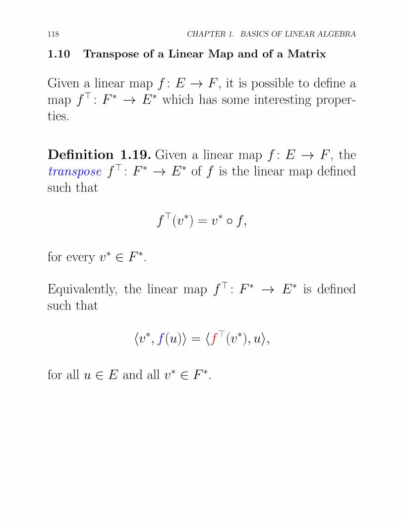
118 CHAPTER 1. BASICS OF LINEAR ALGEBRA
1.10 Transpose of a Linear Map and of a Matrix
Given a linear map f : E → F , it is possible to define amap f� : F ∗ → E∗ which has some interesting proper-ties.
Definition 1.19. Given a linear map f : E → F , thetranspose f� : F ∗ → E∗ of f is the linear map definedsuch that
f�(v∗) = v∗ ◦ f,
for every v∗ ∈ F ∗.
Equivalently, the linear map f� : F ∗ → E∗ is definedsuch that
�v∗, f (u)� = �f�(v∗), u�,
for all u ∈ E and all v∗ ∈ F ∗.

1.10. TRANSPOSE OF A LINEAR MAP AND OF A MATRIX 119
It is easy to verify that the following properties hold:
(f + g)� = f� + g�
(g ◦ f )� = f� ◦ g�
id�E = idE∗.
� Note the reversal of composition on the right-hand sideof (g ◦ f )� = f� ◦ g�.
If E is finite-dimensional and if we identify E with itsbidual E∗∗, then
(f�)� = f.
Proposition 1.29. Given a linear map f : E → F ,for any subspace U of E, we have
f (U)0 = (f�)−1(U 0) = {v∗ ∈ F ∗ | f�(v∗) ∈ U 0}.
As a consequence,
Ker f� = (Im f )0 and Ker f = (Im f�)0.

120 CHAPTER 1. BASICS OF LINEAR ALGEBRA
The following theorem shows the relationship between therank of f and the rank of f�.
Theorem 1.30. Given a linear map f : E → F , thefollowing properties hold.
(a) The dual (Im f )∗ of Im f is isomorphic toIm f� = f�(F ∗); that is,
(Im f )∗ ≈ Im f�.
(b) If F is finite dimensional, then rk(f ) = rk(f�).
The following proposition shows the relationship betweenthe matrix representing a linear map f : E → F and thematrix representing its transpose f� : F ∗ → E∗.

1.10. TRANSPOSE OF A LINEAR MAP AND OF A MATRIX 121
Proposition 1.31. Let E and F be two vector spaces,and let (u1, . . . , un) be a basis for E, and (v1, . . . , vm)be a basis for F . Given any linear map f : E → F ,if M(f ) is the m × n-matrix representing f w.r.t.the bases (u1, . . . , un) and (v1, . . . , vm), the n × m-matrix M(f�) representing f� : F ∗ → E∗ w.r.t. thedual bases (v∗1, . . . , v
∗m) and (u∗1, . . . , u
∗n) is the trans-
pose M(f )� of M(f ).
We now can give a very short proof of the fact that therank of a matrix is equal to the rank of its transpose.
Proposition 1.32. Given a m × n matrix A over afield K, we have rk(A) = rk(A�).
Thus, given an m × n-matrix A, the maximum numberof linearly independent columns is equal to the maximumnumber of linearly independent rows.
Proposition 1.32 immediately yields the following crite-rion for determining the rank of a matrix:

122 CHAPTER 1. BASICS OF LINEAR ALGEBRA
Proposition 1.33.Given any m×n matrix A over afield K (typically K = R or K = C), the rank of A isthe maximum natural number r such that there is aninvertible r × r submatrix of A obtained by selectingr rows and r columns of A.
For example, the 3× 2 matrix
A =
a11 a12a21 a22a31 a32
has rank 2 iff one of the three 2× 2 matrices�a11 a12a21 a22
� �a11 a12a31 a32
� �a21 a22a31 a32
�
is invertible. We will see in Chapter 2 that this is equiv-alent to the fact the determinant of one of the abovematrices is nonzero.
This is not a very efficient way of finding the rank ofa matrix. We will see that there are better ways usingvarious decompositions such as LU, QR, or SVD.

1.11. THE FOUR FUNDAMENTAL SUBSPACES 123
1.11 The Four Fundamental Subspaces
Given a linear map f : E → F (where E and F arefinite-dimensional), Proposition 1.29 revealed that thefour spaces
Im f, Im f�, Ker f, Ker f�
play a special role. They are often called the fundamentalsubspaces associated with f .
These spaces are related in an intimate manner, sinceProposition 1.29 shows that
Ker f = (Im f�)0
Ker f� = (Im f )0,
and Theorem 1.30 shows that
rk(f ) = rk(f�).

124 CHAPTER 1. BASICS OF LINEAR ALGEBRA
It is instructive to translate these relations in terms ofmatrices (actually, certain linear algebra books make abig deal about this!).
If dim(E) = n and dim(F ) = m, given any basis (u1, . . .,un) of E and a basis (f1, . . . , fm) of F , we know that fis represented by an m× n matrix A = (ai j), where thejth column of A is equal to f (ej).
Furthermore, the transpose map f� is represented by then×m matrix A� (with respect to the dual bases).
Consequently, the four fundamental spaces
Im f, Im f�, Ker f, Ker f�
correspond to

1.11. THE FOUR FUNDAMENTAL SUBSPACES 125
(1) The column space of A, denoted by ImA or R(A);this is the subspace of Rm spanned by the columns ofA, which corresponds to image Im f of f .
(2) The kernel or nullspace of A, denoted by KerA orN (A); this is the subspace of Rn consisting of allvectors x ∈ Rn such that Ax = 0.
(3) The row space of A, denoted by ImA� or R(A�);this is the subspace of Rn spanned by the rows of A,or equivalently, spanned by the columns of A�, whichcorresponds to image Im f� of f�.
(4) The left kernel or left nullspace of A denoted byKerA� orN (A�); this is the kernel (nullspace) ofA�,the subspace of Rm consisting of all vectors y ∈ Rm
such that A�y = 0, or equivalently, y�A = 0.
Recall that the dimension r of Im f , which is also equalto the dimension of the column space ImA = R(A), isthe rank of A (and f ).

126 CHAPTER 1. BASICS OF LINEAR ALGEBRA
Then, some our previous results can be reformulated asfollows:
1. The column space R(A) of A has dimension r.
2. The nullspace N (A) of A has dimension n− r.
3. The row space R(A�) has dimension r.
4. The left nullspace N (A�) of A has dimension m− r.
The above statements constitute what Strang calls theFundamental Theorem of Linear Algebra, Part I (seeStrang [28]).

1.11. THE FOUR FUNDAMENTAL SUBSPACES 127
The two statements
Ker f = (Im f�)0
Ker f� = (Im f )0
translate to
(1) The nullspace of A is the orthogonal of the row spaceof A.
(2) The left nullspace ofA is the orthogonal of the columnspace of A.
The above statements constitute what Strang calls theFundamental Theorem of Linear Algebra, Part II (seeStrang [28]).
Since vectors are represented by column vectors and linearforms by row vectors (over a basis in E or F ), a vectorx ∈ Rn is orthogonal to a linear form y if
yx = 0.

128 CHAPTER 1. BASICS OF LINEAR ALGEBRA
Then, a vector x ∈ Rn is orthogonal to the row space ofA iff x is orthogonal to every row of A, namelyAx = 0, which is equivalent to the fact that x belong tothe nullspace of A.
Similarly, the column vector y ∈ Rm (representing alinear form over the dual basis of F ∗) belongs to thenullspace of A� iff A�y = 0, iff y�A = 0, which meansthat the linear form given by y� (over the basis in F ) isorthogonal to the column space of A.
Since (2) is equivalent to the fact that the column spaceof A is equal to the orthogonal of the left nullspace ofA, we get the following criterion for the solvability of anequation of the form Ax = b:
The equation Ax = b has a solution iff for all y ∈ Rm, ifA�y = 0, then y�b = 0.

1.11. THE FOUR FUNDAMENTAL SUBSPACES 129
Indeed, the condition on the right-hand side says that bis orthogonal to the left nullspace of A, that is, that bbelongs to the column space of A.
This criterion can be cheaper to check that checking di-rectly that b is spanned by the columns of A. For exam-ple, if we consider the system
x1 − x2 = b1x2 − x3 = b2x3 − x1 = b3
which, in matrix form, is written Ax = b as below:
1 −1 00 1 −1−1 0 1
x1x2x3
=
b1b2b3
,
we see that the rows of the matrix A add up to 0.

130 CHAPTER 1. BASICS OF LINEAR ALGEBRA
In fact, it is easy to convince ourselves that the left nullspaceof A is spanned by y = (1, 1, 1), and so the system is solv-able iff y�b = 0, namely
b1 + b2 + b3 = 0.
Note that the above criterion can also be stated negativelyas follows:
The equation Ax = b has no solution iff there is somey ∈ Rm such that A�y = 0 and y�b �= 0.


![Vita for Jean H. Gallier 1 Personal Data - University of ...jean/vita2.pdf4 Vita for Jean H. Gallier [15] Building Exact Computation Sequences. (With Alex Pelin). Theoretical Computer](https://static.fdocuments.us/doc/165x107/5ad40abd7f8b9aff228b5c3e/vita-for-jean-h-gallier-1-personal-data-university-of-jeanvita2pdf4-vita.jpg)