Algebra - Information and Computer Sciencejean/algebra.pdfAlgebra by Stephen S. Shatz and Jean...
421
Algebra by Stephen S. Shatz * and Jean Gallier ** * Department of Mathematics ** Department of Computer and Information Science University of Pennsylvania Philadelphia, PA 19104, USA c Stephen S. Shatz & Jean Gallier February 8, 2017
Transcript of Algebra - Information and Computer Sciencejean/algebra.pdfAlgebra by Stephen S. Shatz and Jean...

Algebra
by
Stephen S. Shatz∗ and Jean Gallier∗∗
∗Department of Mathematics∗∗Department of Computer and Information Science
University of PennsylvaniaPhiladelphia, PA 19104, USA
c©Stephen S. Shatz & Jean Gallier
February 8, 2017

ii

iii
To the memories of Peter A. Cassileth, Stanley M.K. Chung, and Ralph C. Marcove,physicians and friends all. Being mortal and denied the gift of life, he gives and they gave
the next best thing: Time.
To Anne, Mia, Philippe and Sylvie

iv

Contents
Preface vii
For the Student ix
Problems 1
1 Group Theory 57
1.1 Introduction . . . . . . . . . . . . . . . . . . . . . . . . . . . . . . . . . . . . . . . . . . . . . . 57
1.2 Group Actions and First Applications; The Three Sylow Theorems . . . . . . . . . . . . . . . 57
1.3 Elementary Theory of p-Groups . . . . . . . . . . . . . . . . . . . . . . . . . . . . . . . . . . . 69
1.4 Group Extensions . . . . . . . . . . . . . . . . . . . . . . . . . . . . . . . . . . . . . . . . . . . 75
1.5 Solvable and Nilpotent Groups . . . . . . . . . . . . . . . . . . . . . . . . . . . . . . . . . . . 88
1.6 Ω-Groups and the Jordan-Holder-Schreier Theorem . . . . . . . . . . . . . . . . . . . . . . . . 92
1.7 Categories, Functors and Free Groups . . . . . . . . . . . . . . . . . . . . . . . . . . . . . . . 95
1.8 Further Readings . . . . . . . . . . . . . . . . . . . . . . . . . . . . . . . . . . . . . . . . . . . 108
2 Rings and Modules 109
2.1 Introduction . . . . . . . . . . . . . . . . . . . . . . . . . . . . . . . . . . . . . . . . . . . . . . 109
2.2 Polynomial Rings, Commutative and Noncommutative . . . . . . . . . . . . . . . . . . . . . . 109
2.3 Operations on Modules; Finiteness Conditions . . . . . . . . . . . . . . . . . . . . . . . . . . . 115
2.4 Projective and Injective Modules . . . . . . . . . . . . . . . . . . . . . . . . . . . . . . . . . . 125
2.5 The Five Lemma and the Snake Lemma . . . . . . . . . . . . . . . . . . . . . . . . . . . . . . 136
2.6 Tensor Products and Flat Modules . . . . . . . . . . . . . . . . . . . . . . . . . . . . . . . . . 139
2.7 Limit Processes in Algebra . . . . . . . . . . . . . . . . . . . . . . . . . . . . . . . . . . . . . 156
2.8 Flat Modules (Again) . . . . . . . . . . . . . . . . . . . . . . . . . . . . . . . . . . . . . . . . 163
2.9 Further Readings . . . . . . . . . . . . . . . . . . . . . . . . . . . . . . . . . . . . . . . . . . . 171
3 Commutative Rings 173
3.1 Introduction . . . . . . . . . . . . . . . . . . . . . . . . . . . . . . . . . . . . . . . . . . . . . . 173
3.2 Classical Localization . . . . . . . . . . . . . . . . . . . . . . . . . . . . . . . . . . . . . . . . 173
3.3 Prime and Maximal Ideals . . . . . . . . . . . . . . . . . . . . . . . . . . . . . . . . . . . . . . 179
3.4 First Applications of Fraction Rings . . . . . . . . . . . . . . . . . . . . . . . . . . . . . . . . 194
3.5 Integral Dependence . . . . . . . . . . . . . . . . . . . . . . . . . . . . . . . . . . . . . . . . . 203
3.6 Primary Decomposition . . . . . . . . . . . . . . . . . . . . . . . . . . . . . . . . . . . . . . . 223
3.7 Theorems of Krull and Artin–Rees . . . . . . . . . . . . . . . . . . . . . . . . . . . . . . . . . 236
3.8 Further Readings . . . . . . . . . . . . . . . . . . . . . . . . . . . . . . . . . . . . . . . . . . . 242
v

vi CONTENTS
4 Fields and Galois Theory 2434.1 Introduction . . . . . . . . . . . . . . . . . . . . . . . . . . . . . . . . . . . . . . . . . . . . . . 2434.2 Algebraic Extensions . . . . . . . . . . . . . . . . . . . . . . . . . . . . . . . . . . . . . . . . . 2434.3 Separable Extensions, Kahler Differentials, Mac Lane’s Criterion . . . . . . . . . . . . . . . . 2484.4 The Extension Lemma and Splitting Fields . . . . . . . . . . . . . . . . . . . . . . . . . . . . 2564.5 The Theorems of Dedekind and Artin; Galois Groups . . . . . . . . . . . . . . . . . . . . . . 2604.6 Primitive Elements, Normal Bases . . . . . . . . . . . . . . . . . . . . . . . . . . . . . . . . . 2704.7 Galois Cohomology, Norms and Traces . . . . . . . . . . . . . . . . . . . . . . . . . . . . . . . 2774.8 Krull’s Galois Theory . . . . . . . . . . . . . . . . . . . . . . . . . . . . . . . . . . . . . . . . 2844.9 Kummer Theory . . . . . . . . . . . . . . . . . . . . . . . . . . . . . . . . . . . . . . . . . . . 2894.10 An Amazing Theorem of Galois Theory . . . . . . . . . . . . . . . . . . . . . . . . . . . . . . 2944.11 Algebraic Closures; Steinitz’s Theory of Fields . . . . . . . . . . . . . . . . . . . . . . . . . . 2984.12 Further Readings . . . . . . . . . . . . . . . . . . . . . . . . . . . . . . . . . . . . . . . . . . . 308
5 Homological Algebra 3095.1 Introduction . . . . . . . . . . . . . . . . . . . . . . . . . . . . . . . . . . . . . . . . . . . . . . 3095.2 Complexes, Resolutions, Derived Functors . . . . . . . . . . . . . . . . . . . . . . . . . . . . . 3095.3 Various (Co)homological Functors . . . . . . . . . . . . . . . . . . . . . . . . . . . . . . . . . 3275.4 Spectral Sequences; First Applications . . . . . . . . . . . . . . . . . . . . . . . . . . . . . . . 3555.5 The Koszul Complex and Applications . . . . . . . . . . . . . . . . . . . . . . . . . . . . . . . 3785.6 Concluding Remarks . . . . . . . . . . . . . . . . . . . . . . . . . . . . . . . . . . . . . . . . . 3975.7 Supplementary Readings . . . . . . . . . . . . . . . . . . . . . . . . . . . . . . . . . . . . . . . 397

Preface
A book on “Abstract” or “Modern” Algebra is a commonplace thing in today’s mathematical milieu. Even abook for well-prepared, serious beginning graduate students who intend to become research mathematiciansis not so strange any longer. But, the genesis of this book, which is intended for serious, well-preparedgraduate students, is somewhat strange.
To begin with, it is a reworking of notes for a year long graduate course I gave several years ago–notin itself a strange thing. But, I possess no such notes nor did I ever make any and I never lecture with awritten aide memoir of any sort. Rather, my method is to work out fully during lecture (at the board) eachproof and example. Students will thus see what are the “inner workings” of the subject. Of course, this ispedagogically to their advantage and, furthermore, it slows me down.
Then where did the notes (to be reworked) come from? They were provided by my friend and colleagueJean H. Gallier (of the Computer Science Department at Penn). Determined to augment his mathematicalknowledge, he began several years ago to audit some of my graduate courses. “Audit” for him meansfaithfully attending lectures, doing all the problem assignments, participating in each bi-weekly problemsession (where he takes his turn presenting problems), writing excellent notes from my oral presentation andrendering these notes in LATEX form.1 That this book will appear is, in large measure, his doing. While Ihave been responsible for its writing, he has on occasion introduced results and/or alternate proofs that haverendered some material more perspicacious from a student’s point of view–these have improved the text. Heis in every sense a joint author, save that errors are solely my responsibility. There is no way I can thankhim adequately here in plain words and I won’t try except to say, Je te remercie vivement, mon ami Jean,pour tout ton travail .
Others should be thanked as well–in particular the members of the class that attended the course fromwhich the book is formed.2 By their interest and attention to detail, they kept me on my toes. Oneparticular member of that class deserves special mention: Mathew Cross.3 Mathew started the index andset the original 115 problems in LATEX. He lightened our burden by a considerable amount.
The content of the book follows rather closely the oral lectures–with just a few exceptions. These are: InChapter 3, the section on Integral Dependence is now augmented by proofs of all results, the original lectureshad statements only of some of these (due to exigencies of time) and Gallier insisted on a full treatment.In Chapter 4, the sections on Norms and Traces as well as Kummer Theory and Transcendental Extensionsare likewise augmented by full proofs. In Chapter 5, there is now more to the section on (co)homologicalfunctors and there are full proofs in the last section on the Koszul Complex. Otherwise, the material is just(a smoothed out version of) what was presented. One will have to move fast to present it to students in oneyear, at least I did.
But the heart of the book is the Problem section. Here, I’ve attempted to simulate at the beginninggraduate level some of the features of real mathematical work. There is a jumbling of the problems vis a
1One must realize he maintains a full research and teaching schedule, directs Ph.D. students, attends to administrative dutiesand has a family life in addition to this “auditing”!
2The members of the class were: A. Bak, D. Boyarchenko, S. Brooks, M. Campbell, S. Corry, M. Cross, C. Daenzer, C.Devena, J. Gallier, S. Guerra, C. Hoelscher, T. Jaeger, J. Long, S. Mason, T. Zhu.
3Mathew spells his name with but one “t”; there is no misprint.
vii

viii Preface
vis subject matter just as in real research one never knows what kind of mathematics will be needed in thesolution of a problem. There is no hint of the level of difficulty of a problem (save for the few problemswhere suggestions are offered), and anyway the notion of difficulty is ill-defined. And, the problems refer toeach other, just as in real work one is constantly reminded of past efforts (successful or not). In effect, assuggested in the preface for students, one should begin with the problems and use the text as a means tofill in knowledge as required to do them (as well as to do other problems assigned by an instructor in thiscourse or another course).
This brings me to the text material itself. There is no attempt to be encyclopedic. After all, the materialis a faithful copy of what was actually covered in a year and any competent instructor can add materialthat has been omitted. I regret not covering the Wederburn-Artin Theory of DCC rings, the Brauer Group,and some basic material on group representations. What is covered, however, is to my mind central tothe education of any prospective mathematician who aspires to contribute to what is now the mainstreamof mathematical endeavor. Also, while there are over 150 problems filling some 55 pages of text (some ofthe problems are rather long being multi-part), other problems of an instructor’s choosing can certainly beassigned. As to the attribution of the origins of these problems, I have assigned names when they are knownto me. If no name is assigned, the problem comes from some source in my past (perhaps one of my ownteachers or their teachers) and in no way do I claim it as my own. Good problems from all sources are thetreasure hoard of practicing mathematicians in their role as passers on of our common heritage.
I refer to the special symbols (DX) and the “curves ahead” road sign (appearing at odd places in thetext) in the student preface; no repeat of the explanations I offer there is necessary. If you as instructor arelucky enough to have a class as interested and tough to satisfy as I did, you are lucky indeed and need nofurther assurance that mathematics will be in good hands in the future. I intend this book to be of serviceto such individuals as they begin their long climb to mathematical independence and maturity.
Tolda Santa CotognaSummer, 2006

For the Student
It may be surprising but the most important part of the book you now hold before you is the very firstsection–the one labeled “Problems.” To learn mathematics one must do mathematics. Indeed, the bestway to read this book is to turn immediately to the problem section and begin to do the problems. Ofcourse, you will soon reach some unknown terminology or not have enough knowledge to meet the technicaldemands of a problem and this is where you turn to the text to fill in gaps, see ideas explained and techniquesdemonstrated. Then you plunge once more back into the problems and repeat the whole process.
The book is designed for serious, well-prepared students who plan on becoming research mathematicians.It presumes you have had previous acquaintance with algebra; in particular you have met the concepts ofgroup, ring, field, vector space, homomorphism, isomorphism, and the elementary theorems about thesethings. No book on mathematics can be simply read, rather you must recreate the text yourself line by linechecking at each stage all details including those omitted. This is slow work and, as you know, mathematicshas very high density on the page.
In the text, you will find two special symbols: (DX) and a sign such as one sees on the road warningof dangerous curves ahead. The symbol (DX) stands for “diagnostic exercise”, it means some elementarydetails have been omitted and that supplying them should be easy. However, if supplying them is not easy,then you should go back a page or two as something fundamental has skipped you by. In this way, the sign(DX) is like a medical test: failing it is sure to tell you if something is wrong (no false positives), however,if you pass it (supply the details), something still might be wrong. Just read on and anything wrong willsurface later. As for the dangerous curves sign, it precedes counter-examples to naively made conjectures, itwarns when things could go wrong if hypotheses are omitted, and generally forces you to slow down in thereading and recreating.
If you use this book in a course or even for self study, I recommend that you tackle the problems in asmall group (two to four persons, total). This is because no person has a monopoly on ideas, a good ideaor half-idea can germ in any head, and the working out of a problem by a committed group is akin to theactual way much research mathematics is accomplished. In your group, you want constant give and take,and there must be time to think alone so that a real contribution to the group’s effort can be made.
The problems are all jumbled up by area and there is no signal given as to a problem’s difficulty (exceptionsare the few cases where hints or suggestions are given). In real mathematical life, no signs are given that aquestion being attacked involves a certain small area of mathematical knowledge or is hard or easy; any suchsign is gleaned by virtue of experience and that is what you are obtaining by doing mathematics in theseproblems. Moreover, hard and easy are in the eyes of the beholder; they are not universal characteristicsof a problem. About all one can say is that if a large number of people find a problem difficult, we mayclassify it so. However, we shouldn’t be surprised when an individual solves it and claims that, “it was notthat hard”. In any case, guard against confusing mathematical talent either with overall intelligence or withmathematical speed. Some quick people are in fact talented, many are just quick. Don’t be discouraged ifyou find yourself slower than another, the things that really count in doing mathematics (assuming talent)are persistence and courage.
ix

x For the Student
I can think of no better lines to close with than these which come from B. Pasternak’s poem entitled“Night”4
“And maybe in an atticAnd under ancient slatesA man sits wakeful workingHe thinks and broods and waits.”
“He looks upon the planet,As if the heavenly spheresWere part of his entrustedNocturnal private cares.”
“Fight off your sleep: be wakeful,Work on, keep up your pace,Keep vigil like the pilot,Like all the stars in space.”
“Work on, work on, creator–To sleep would be a crime–Eternity’s own hostage,And prisoner of Time.”
Tolda Santa CotognaSummer, 2006
4From the collection entitled “When It Clears Up”, 1956. Translated by Lydia Pasternak Slater (the poet’s sister).

Problems
“... den Samen in den Wind streuend; fasse, wer es fassen kann”.
—Hermann Weyl
Problem 1
1. Suppose G is a finite group and that AutGr(G) = 1. (Here, AutGr(G) is the group of all bijections,G→ G, which are also group homomorphisms.) Find all such groups G.
2. Write Z/2Z for the cyclic group of order 2. If G = Z/2Z∏ · · · ∏ Z/2Z, t-times, compute
#(AutGr(G)
). When t = 2, determine the group AutGr(G). When t = 3, determine the struc-
ture of the odd prime Sylows. Can you decide whether AutGr(G) has any normal subgroups in thecase t = 3?
Problem 2
1. (Poincare). In an infinite group, prove that the intersection of two subgroups of finite index has finiteindex itself.
2. Show that if a group, G, has a subgroup of finite index, then it possesses a normal subgroup of finiteindex. Hence, an infinite simple group has no subgroups of finite index.
3. Sharpen (2) by proving: if (G : H) = r, then G possesses a normal subgroup, N , with (G : N) ≤ r!.Conclude immediately that a group of order 36 cannot be simple.
Problem 3 Let G = GL(n,C) and ∆n be the subgroup of matrices with entries only along the diagonal.Describe precisely NG(∆n) in terms of what the matrices look like.
Problem 4 Say G is a group and #(G) = prg0, where p is a prime and (p, g0) = 1. Assume
r >
g0−1∑
j=1
∑
k>0
[j/pk]
([x] = largest integer ≤ x
). Prove that G is not simple. Show that this governs all groups of order < 60,
except for #(G) = 30, 40, 56. We know that #(G) = 30 =⇒ G not simple. Show by explicit argument thatgroups of orders 40, 56 are not simple. (Here, of course, by simple we mean non-abelian and simple.)
Problem 5 In a p-group, G, we cannot have
(G : Z(G)) = p.
Show that for non-abelian groups of order p3, Z(G) ∼= Z/pZ and G/Z(G) ∼= Z/pZ∏
Z/pZ.
1

2 PROBLEMS
Problem 6 Let G be the group of automorphisms of a regular polyhedron with v vertices, e edges, and ffaces. Show that G has order g = fs = vr = 2e, where s is the number of sides to a face and r is the numberof edges emanating from a vertex. From topology, one knows Euler’s formula
v − e+ f = 2.
Find the only possible values for v, e, f, r, s, g. Make a table.
Problem 7 Let p be a prime number. Find all non-abelian groups of order p3. Get started with theBurnside basis theorem, but be careful to check that the groups on your list are non-isomorphic. Also makesure your list is exhaustive. Your list should be a description of the generators of your groups and therelations they satisfy.
Problem 8 Let G be a finite group and write c(G) for the number of distinct conjugacy classes in G. Thisnumber will increase (in general) as #(G)→∞; so, look at
c(G) =c(G)
#(G).
The number c(G) measures the “average number of conjugacy classes per element of G” and is 1 if G isabelian. Assume G is non-abelian from now on. Then 0 < c(G) < 1.
1. Prove that for all such G, we have c(G) ≤ 5/8.
2. Suppose p is the smallest prime with p |#(G). Prove that
c(G) ≤ 1
p+
1
p2− 1
p3.
Is the bound of (1) sharp; that is, does there exist a G with c(G) = 5/8? How about the bound of (2)?
Problem 9 If G is a finite group and H a normal subgroup of G, write P for a p-Sylow subgroup of H.
1. Show that the natural injectionNG(P )/NH(P )→ G/H
(why does it exist, why injective?) is actually an isomorphism.
2. Prove that the Frattini subgroup, Φ(G), of ANY finite group, G, has property N (cf. Section 1.3,Chapter 1).
Problem 10 We’ve remarked that Φ(G) is a kind of “radical” in the group-theoretic setting. In this problemwe study various types of radicals.A normal subgroup, H, of G is called small iff for every XCG, the equality H ·X = G implies that X = G.(Note: 1 is small, Φ(G) is small; so they exist.) Check that if H and L are small, so is HL, and if H issmall and K CG, then K ⊆ H =⇒ K is small.
1. The small radical of G, denoted J ∗∗(G), is
J ∗∗(G) =x ∈ G
∣∣GpCl(x) is small.
(Here, Cl(x) is the conjugacy class of x in G, and GpS is the group generated by S.) Prove thatJ ∗∗(G) is a subgroup of G.
2. The Jacobson radical of G, denoted J ∗(G), is the intersection of all maximal, normal subgroups of G;while the Baer radical of G, denoted J (G), is the product (inside G) of all the small subgroups of G.Prove
J ∗∗(G) ⊆ J (G) ⊆ J ∗(G).

PROBLEMS 3
3. Prove Baer’s Theorem: J ∗∗(G) = J (G) = J ∗(G). (Suggestion: if x 6∈ J ∗∗(G), find N CG (6= G) sothat GpCl(x)N = G. Now construct an appropriate maximal normal subgroup not containing x.)
Problem 11 Recall that a characteristic subgroup is one taken into itself by all automorphisms of thegroup.
1. Prove that a group possessing no proper characteristic subgroups is isomorphic to a product of iso-morphic simple groups. (Hints: Choose G of smallest possible order (> 1) normal in G. Consider all
subgroups, H, for which H ∼= G1
∏ · · · ∏ Gt, where each Gj CG and each Gj ∼= G. Pick t so that#(H) is maximal. Prove that H is characteristic. Show K CG1 (say) =⇒ K CG.)
2. Prove: In every finite group, G, a minimal normal subgroup, H, is either an elementary abelian p-groupor is isomorphic to a product of mutually isomorphic, non-abelian, simple groups.
3. Show that in a solvable group, G, only the first case in (2) occurs.
Problem 12 Let G be a finite p-group and suppose ϕ ∈ Aut(G) has order n (i.e., ϕ(ϕ(· · · (ϕ(x)) · · · )
)= Id,
all x ∈ G: we do ϕ n-times in succession and n is minimal). Suppose (n, p) = 1. Now ϕ induces anautomorphism of G/Φ(G), call it ϕ, as Φ(G) is characteristic. Remember that G/Φ(G) is a vector spaceover Fp; so, ϕ ∈ GL
(G/Φ(G)
).
1. Prove ϕ = identity ⇐⇒ ϕ = identity.
2. Show that if d is the Burnside dimension of G, then
#(GL(G/Φ(G))
)= p
d(d−1)2
d∏
k=1
(pk − 1),
and that if P is a p-Sylow subgroup of GL(G/Φ(G)
), then P ⊆ SL
(G/Φ(G)
); i.e., σ ∈ P =⇒
det(σ) = 1.
3. Let P = ϕ ∈ Aut(G) | ϕ ∈ P, no restriction on the order of ϕ. Show that P is a p-subgroup ofAut(G).
4. Call an element σ ∈ GL(G/Φ(G)
)liftable iff it is ϕ for some ϕ ∈ Aut(G). Examine all G of order
p, p2, p3 to help answer the following: Is every σ liftable? If not, how can you tell (given σ) if σ isliftable?
Problem 13 Let p be a prime number and consider a set, S, of p objects: S = α1, . . . , αp. Assume Gis a transitive group of permutations of S (i.e., the elements of S form an orbit under G); further assume(α1α2) ∈ G (here (α1α2) is the transposition). Prove: G = Sp. (Suggestion: let M = αj |(α1αj) ∈ G,show if σ ∈ Sp and σ = 1 outside M then σ ∈ G. Now prove #(M)| p.)
Problem 14 A Fermat prime, p, is a prime number of the form 2α + 1. E.g., 2, 3, 5, 17, 257, . . ..
1. Show if 2α + 1 is prime then α = 2β .
2. Say p is a Fermat prime (they are quite big) and g0 is an odd number with g0 < p. Prove that anygroup of order g0p is isomorphic to a product G0
∏(Z/pZ), where #(G0) = g0. Hence, for example,
the groups of orders 51(= 3 ·17), 85(= 5 ·17), 119(= 7 ·17), 153(= 9 ·17), 187(= 11 ·17), 221(= 13 ·17),255(= 3 · 5 · 17) are all abelian. Most we knew already, but 153 = 32 · 17 and 255 = 3 · 5 · 17 are new.
3. Generalize to any prime, p, and g0 < p, with p 6≡ 1 mod g0. For example, find all groups of order 130.
Problem 15 Recall that a group, G, is finitely generated (f.g.) iff (∃σ1, . . . , σn ∈ G)(G = Gpσ1, . . . , σn).

4 PROBLEMS
1. If G is an abelian f.g. group, prove each of its subgroups is f.g.
2. In an arbitrary group, G, an element σ ∈ G is called n-torsion (n ∈ N) ⇐⇒ σn = 1; σ is torsion iffit is n-torsion for some n ∈ N. The element σ ∈ G is torsion free ⇐⇒ it is not torsion. Show that inan abelian group, the set
t(G) = σ ∈ G | σ is torsion
is a subgroup and that G/t(G) is torsion free (i.e., all its non-identity elements are torsion free).
3. In the solvable group 0→ Z→ G→ Z/2Z→ 0 (split extension, non-trivial action) find two elements
x, y satisfying: x2 = y2 = 1 and xy is torsion free. Can you construct a group, G, possessing elementsx, y of order 2, so that xy has order n, where n is predetermined in N? Can you construct G solvablewith these properties?
4. Back to the abelian case. If G is abelian and finitely generated show that t(G) is a finite group.
5. Say G is abelian, f.g., and torsion-free. Write d for the minimal number of generators of G. Prove thatG is isomorphic to a product of d copies of Z.
6. If G is abelian and f.g., prove that
G ∼= t(G)∏(
G/t(G)).
Problem 16 Let (P) be a property of groups. We say a group, G, is locally (P) ⇐⇒ each f.g. subgroupof G has (P). Usually, one says a locally cyclic group is a rank one group.
1. Prove that a rank one group is abelian.
2. Show that the additive group of rational numbers, Q+, is a rank one group.
3. Show that every torsion-free, rank one group is isomorphic to a subgroup of Q+.
Problem 17 Fix a group, G, and consider the set, Mn(G), of n × n matrices with entries from G orso that αij = 0 (i.e., entries are 0 or from G). Assume for each row and each column there is one andonly one non-zero entry. These matrices form a group under ordinary “matrix multiplication” if we define0 · group element = group element · 0 = 0. Establish an isomorphism of this group with the wreath productGn oSn. As an application, for the subgroup of GL(n,C) consisting of diagonal matrices, call it ∆n, showthat
NG(∆n) ∼= Cn oSn, here G = GL(n,C).
Problem 18
1. Say G is a simple group of order n and say p is a prime number dividing n. If σ1, . . . , σt is a listing ofthe elements of G of exact order p, prove that G = Gpσ1, . . . , σt.
2. Suppose G is any finite group of order n and that d is a positive integer relatively prime to n. Showthat every element of G is a dth power.
Problem 19 We know that when G is a (finite) cyclic group, and A is any G-module, we have an isomor-phism
AG/N (A)∼−→ H2(G,A).
This problem is designed to lead to a proof. There are other proofs which you might dig out of books (aftersome effort), but do this proof.

PROBLEMS 5
1. Suppose G is any group and A, B, C are G-modules. Suppose further, we are given a G-pairing ofA∏B → C i.e., a map
θ : A∏
B → C
which is bi-additive and “G-linear”:σθ(a, b) = θ(σa, σb).
If f , g are r-, s-cochains of G with values in A, B (respectively), we can define an (r + s)-cochain ofG with values in C via the formula:
(f `θ g)(σ1, . . . , σr, σr+1, . . . , σr+s) = θ(f(σ1, . . . , σr), σ1 . . . σrg(σr+1, . . . , σr+s)
).
Prove that δ(f `θ g) = δf `θ g + (−1)rf `θ δg. Show how you conclude from this that we have apairing of abelian groups
`θ: Hr(G,A)
∏Hs(G,B)→ Hr+s(G,C).
(Notation and nomenclature: α `θ β, cup-product.)
2. Again G is any group, this time finite. Let Z and Q/Z be G-modules with trivial action. Consider
the abelian group Homgr(G,Q/Z) = G, where addition in G is by pointwise operation on functions. If
χ ∈ G, then χ(σ) ∈ Q/Z, all σ ∈ G. Show that the function
fχ(σ, τ) = δχ(σ, τ) = σχ(τ)− χ(στ) + χ(σ)
has values in Z and actually is a 2-cocycle with values in Z. (This is an example of the principle: If itlooks like a coboundary, it is certainly a cocycle.) The map
χ ∈ G 7→ cohomology class of fχ(σ, τ) (†)
gives a homomorphism G→ H2(G,Z).Now any 2-cocycle g(σ, τ) with values in Z can be regarded as a 2-cocycle with values in Q (corre-sponding to the injection Z → Q). Show that as a 2-cocycle in Q it is a coboundary (of some h(σ),values in Q). So, g(σ, τ) = δh(σ, τ), some h. Use this construction to prove:
For any finite group, G, the map (†) above gives an isomorphism of G with H2(G,Z).
3. Now let G be finite, A be any G-module, and Z have the trivial G-action. We have an obvious G-pairingZ∏A→ A, namely (n, a) 7→ na, hence by (1) and (2) we obtain a pairing
G(= H2(G,Z))∏
AG → H2(G,A).
Show that if ξ = Nα, for α ∈ A, then (χ, ξ) goes to 0 in H2(G,A); hence, we obtain a pairing:
G∏
(AG/NA)→ H2(G,A).
(Hint: If f(σ, τ) is a 2-cocycle of G in A, consider the 1-cochain uf (τ) =∑σ∈G f(σ, τ). Using the
cocycle condition and suitable choices of the variables, show the values of uf are in AG and that uf isrelated to N f , i.e., N f(τ, ρ) =
∑σ σf(τ, ρ) can be expressed by uf .)
4. Finally, when G is cyclic, we pick a generator σ0. There exists a distinguished element, χ0, of Gcorresponding to σ0, namely χ0 is that homomorphism G→ Q/Z whose value at σ0 is 1
n modZ, wheren = #(G). Show that the map
AG/NA→ H2(G,A)
viaα 7→ (χ0, α) 7→ δχ0 ` α ∈ H2(G,A)
is the required isomorphism. For surjectivity, I suggest you consider the construction of uf in part (3)above.

6 PROBLEMS
Problem 20 Let G = SL(2,Z) be the group of all 2 × 2 integral matrices of determinant 1; pick a prime,p, and write U for the set of 2 × 2 integral matrices having determinant p. G acts on U via u(∈ U) 7→ σu,where σ ∈ G.
1. Show that the orbit space has p+ 1 elements: 0, 1, . . . , p− 1,∞, where j corresponds to the matrix
wj =
(1 j0 p
)
and ∞ corresponds to the matrix w∞ =
(p 00 1
).
2. If τ ∈ G and r ∈ S = 0, 1, . . . , p − 1,∞ = G\U , show there exists a unique r′ ∈ S with wrτ−1 in
the orbit of wr′ . Write τ · r = r′ and prove this gives an action of G on S. Hence, we have a grouphomomorphism P : G→ Aut(S) = Sp+1.
3. If N = kerP , prove that G/N is isomorphic to the group PSL(2,Fp) consisting of all “fractional lineartransformations”
x 7→ x′ =ax+ b
cx+ d, a, b, c, d ∈ Fp, ad− bc = 1.
Show further that
i. #(PSL(2,Fp)
)=
p(p+ 1)(p− 1)
2if p 6= 2
6 if p = 2
and
ii. PSL(2,Fp) acts transitively on S under the action of (2).
4. Now prove: PSL(2,Fp) is simple if p ≥ 5. (Note: PSL(2,F3) is A4, PSL(2,F5) is A5, but PSL(2,Fp) isnot An if p ≥ 7. So, you now have a second infinite collection of simple finite groups—these are finitegroup analogs of the Lie groups PSL(2,C)).
Problem 21 We write PSL(2,Z) for the group SL(2,Z)/(±I).
(1) Let ξ be a chosen generator for Z/3Z and η the generator of Z/2Z. Map Z/3Z and Z/2Z to PSL(2,Z)via
ϕ(ξ) = x =
(0 −11 1
)(mod ± I)
and
ψ(η) = y =
(0 −11 0
)(mod ± I)
Then we obtain a map
ϕq ψ : Z/3Zq Z/2Z −→ PSL(2,Z)
(here, the coproduct is in the category Grp). What is the image of ϕq ψ? What is the kernel?
(2) If
a =
(1 10 1
)and b =
(1 01 1
)in PSL(2,Z)
express x and y above (in SL(2,Z)) in terms of a and b and show that SL(2,Z) = Grpa, b. Can you expressa and b in terms of x and y?

PROBLEMS 7
(3) For any odd prime number, p, the element
σ(p) =
(1 p−1
20 1
)
is equal to a(p−1)/2. For any σ ∈ SL(2,Z), we define the weight of σ with respect to a and b by
wt(σ) = inf(length of all words in a, b, a−1, b−1, which words equal σ)
By deep theorems of Selberg, Margulis and others (in geometry and analysis) one knows that
wt(σ(p)) = O(log p) as p→∞.
(Our expression for σ(p) as a power of a shows that we have a word of size O(p) for σ(p), yet no explicit wordof size O(log p) is known as of now (Fall, 2005) and the role of b in this is very mysterious.) Now the Cayleygraph of a group, G, generated by the elements g1, . . . , gt is that graph whose vertices are the elements of Gand whose edges emanating from a vertex τ ∈ G are the ones connecting τ and τg1, . . . , τgt. Show that thediameter of the Cayley graph of the group SL(2,Z/pZ) with respect to the generators a and b is O(log p).
Problem 22 Let G be a finite group in this problem.
1. Classify all group extensions0→ Q→ G → G→ 0. (E)
Your answer should be in terms of the collection of all subgroups of G, say H, with (G : H) ≤ 2, plus,perhaps, other data.
2. Same question as (1) for group extensions
0→ Z→ G → G→ 0, (E)
same kind of answer.
3. Write V for the “four-group” Z/2Z∏
Z/2Z. There are two actions of Z/2Z on V : Flip the factors,take each element to its inverse. Are these the only actions? Find all group extensions
0→ V → G → Z/pZ→ 0. (E)
The group G is a group of order 8; compare your results with what you know from Problems 1–6.
4. Say H is any other group, G need no longer be finite and A, B are abelian groups. Suppose ϕ : H → Gis a homomorphism and we are given a group extension
0→ A→ G → G→ 0. (E)
Show that, in a canonical way, we can make a group extension
0→ A→ G → H → 0. (ϕ∗E)
(Note: your answer has to be in terms of G, H, G and any homomorphisms between them as these arethe only “variables” present. You’ll get the idea if you view an extension as a fibre space.)
Now say ψ : A→ B is a group homomorphism and we are given an extension
0→ A→ G → G→ 0. (E)
Construct, in a canonical way, an extension
0→ B → G → G→ 0. (ψ∗E)

8 PROBLEMS
5. Explain, carefully, the relevance of these two constructions to parts (1) and (2) of this problem.
Problem 23 Say A is any abelian group, and write G for the wreath product An oSn. Show:
1. [G,G] 6= G
2.(G : [G,G]
)=∞ ⇐⇒ A is infinite
3. If n ≥ 2, then [G,G] 6= 1.
4. Give a restriction on n which prevents G from being solvable.
Problem 24 If Gαα∈Λ is a family of abelian groups, write∐
α
Gα for
∐
α
Gα =
(ξα) ∈
∏
α
Gα | for all but finitely many α, we have ξα = 0
.
Then∐αGα is the coproduct of the Gα in Ab. Write as well
(Q/Z)p = ξ ∈ Q/Z | prξ = 0, some r > 0;
here, p is a prime. Further, call an abelian group, A, divisible iff
(∀n)(An−→ A→ 0 is exact).
Prove: Theorem Every divisible (abelian) group is a coproduct of copies of Q and (Q/Z)p for various primesp. The group is torsion iff no copies of Q appear, it is torsion-free iff no copies of (Q/Z)p appear (any p).Every torsion-free, divisible, abelian group is naturally a vector space over Q.
Problem 25
1. If G is a group of order n, show that G oAut(G) is isomorphic to a subgroup of Sn.
2. Consider the cycle (1, 2, . . . , n) ∈ Sn; let H be the subgroup (of Sn) generated by the cycle. Provethat
NSn(H) ∼= (Z/nZ) oAut(Z/nZ).
Problem 26 Let TOP denote the category of topological spaces.
1. Show that TOP possesses finite fibred products and finite fibred coproducts.
2. Is (1) true without the word “finite”?
3. Write T2TOP for the full subcategory of TOP consisting of Hausdorff topological spaces. Are (1) and(2) true in T2TOP? If you decide the answer is “no”, give reasonable conditions under which a positiveresult holds. What relation is there between the product (coproduct) you constructed in (1) (or (2))and the corresponding objects in this part of the problem?
Problem 27 Let R be a ring (not necessarily commutative) and write Mod(R) for the category of (left)R-modules; i.e., the action of R on a module, M , is on the left. We know Mod(R) has finite products andfinite fibred products.
1. What is the situation for infinite products and infinite fibred products?
2. What is the situation for coproducts (finite or infinite) and for fibred coproducts (both finite andinfinite)?

PROBLEMS 9
Problem 28 As usual, write Gr for the category of groups. Say G and G′ are groups and ϕ : G → G′ isa homomorphism. Then (G,ϕ) ∈ GrG′ , the comma category of “groups over G′”. The group 1 possess acanonical morphism to G′, namely the inclusion, i. Thus,
(1, i
)∈ GrG′ , as well. We form their product in
GrG′ , i.e., we form the fibred product G∏G′1. Prove that there exists a canonical monomorphism
G∏
G′
1 → G.
Identify its image in G.Now consider the “dual” situation: G′ maps to G, so G ∈ GrG
′(via ϕ) the “groups co-over G′”. We also have
the canonical map G′ → 1, killing all the elements of G′; so, as above, we can form the fibred coproduct
of G and 1: GG′
q 1. Prove that there exists a canonical epimorphism
G→ GG′
q 1,
identify its kernel in G.
Problem 29 Write CR for the category of commutative rings with unity and RNG for the category of ringswith unity.
1. Consider the following two functors from CR to Sets:
(a) |Mpq| : A underlying set of p× q matrices with entries from A
(b) |GLn| : A underlying set of all invertible n× n matrices with entries from A.
Prove the these two functors are representable.
2. A slight modification of (b) above yields a functor from CR to Gr: namely,
GLn : A group of all invertible n× n matrices with entries from A.
When n = 1, we can extend this to a functor from RNG to Gr. That is we get the functor
Gm : A group of all invertible elements of A.
Prove that the functor Gm has a left adjoint, let’s temporarily call it (†); that is: There is a functor(†) from Gr to RNG, so that
(∀G ∈ Gr)(∀R ∈ RNG)(HomRNG((†)(G), R) ∼= HomGr(G,Gm(R))),
via a functorial isomorphism.
3. Show that without knowing what ring (†)(G) is, namely that it exists and that (†) is left adjoint to Gm,we can prove: the category of (†)(G)-modules,Mod
((†)(G)
), is equivalent—in fact isomorphic—to the
category of G-modules.
4. There is a functor from Gr to Ab, namely send G to Gab = G/[G,G]. Show this functor has a rightadjoint, call it I. Namely, there exists a functor I : Ab→ Gr, so that
(∀G ∈ Gr)(∀H ∈ Ab)(HomGr(G, I(H)) ∼= HomAb(Gab, H)).
Does G Gab have a left adjoint?

10 PROBLEMS
Problem 30 (Kaplansky) If A and B are 2×2-matrices with entries in Z, we embed A and B into the 4×4matrices as follows:
Aaug =
(0 IA 0
)
Baug =
(0 IB 0
).
Is it true that if Aaug and Baug are similar over Z, then A and B are similar over Z? Proof or counter-example. What about the case where the entries lie in Q?
Problem 31 We fix a commutative ring with unity, A, and write M for Mpq(A), the p× q matrices withentries in A. Choose a q × p matrix, Γ, and make M a ring via:
Addition: as usual among p× q matricesMultiplication: if R,S ∈M, set R ∗ S = RΓS, where RΓS is the ordinary product of matrices.
Write M(Γ) for M with these operations, then M(Γ) is an A-algebra (a ring which is an A-module).
1. Suppose that A is a field. Prove that the isomorphism classes of M(Γ)’s are finite in number (herep and q are fixed while Γ varies); in fact, are in natural one-to-one correspondence with the integers0, 1, 2, . . . , B where B is to be determined by you.
2. Given two q × p matrices Γ and Γ we call them equivalent iff Γ = WΓZ, where W ∈ GL(q, A) andZ ∈ GL(p,A). Prove: each Γ is equivalent to a matrix
(Ir 00 H
)
where Ir = r× r identity matrix and the entries of H are non-units of A. Is r uniquely determined byΓ? How about the matrix H?
3. Call the commutative ring, A, a local ring provided it possesses exactly one maximal ideal, mA. Forexample, any field is a local ring; the ring Z/pnZ is local if p is a prime; other examples of this large,important class of rings will appear below. We have the descending chain of ideals
A ⊇ mA ⊇ m2A ⊇ · · · .
For some local rings one knows that⋂
t≥0
mtA = (0); let’s call such local rings “good local rings” for
temporary nomenclature. If A is a good local ring, we can define a function on A to Z ∪ ∞, call itord, as follows:
ord(ξ) = 0 if ξ 6∈ mAord(ξ) = n if ξ ∈ mnA but ξ 6∈ mn+1
A
ord(0) =∞.
The following properties are simple to prove:
ord(ξ ± η) ≥ minord(ξ), ord(η)ord(ξη) ≥ ord(ξ) + ord(η).
Consider the q × p matrices under equivalence and look at the following three conditions:
(i) Γ is equivalent to
(Ir 00 H
), with H = (0)

PROBLEMS 11
(ii) Γ is equivalent to
(Ir 00 H
)with H having non-unit entries and r ≥ 1
(iii) (∃Q ∈M)(ΓQΓ = Γ).
Of course, i. =⇒ ii. if Γ 6= (0), A any ring. Prove: if A is any (commutative) ring then i. =⇒ iii., andif A is good local i. and iii. are equivalent. Show further that if A is good local then M(Γ) possessesa non-trivial idempotent, P , (an element such that P ∗ P = P , P 6= 0, 6= 1) if and only if Γ has ii.
4. Write I = U ∈M(Γ) | ΓUΓ = 0 and given P ∈M(Γ), set
B(P ) = V ∈M(Γ) | (∃Z ∈M(Γ))(V = P ∗ Z ∗ P ).
If iii. above holds, show there exists P ∈M(Γ) so that P ∗ P = P and ΓPΓ = Γ. For such a P , provethat B(P ) is a subring of M(Γ), that M(Γ) ∼= B(P ) q I in the category of A-modules, and that Iis a two-sided ideal of M(Γ) (by exhibiting I as the kernel of a surjective ring homomorphism whoseimage you should find). Further show if i. holds, then B(P ) is isomorphic to the ring of r× r matriceswith entries from A. When A is a field show I is a maximal 2-sided ideal of M(Γ), here Γ 6= (0). Is Ithe unique maximal (2-sided) ideal in this case?
5. Call an idempotent, P , of a ring maximal (also called principal) iff when L is another idempotent,then PL = 0 =⇒ L = 0. Suppose Γ satisfies condition iii. above, prove that an idempotent, P , ofM(Γ) is maximal iff ΓPΓ = Γ.
Problem 32 Let A be the field of real numbers R and conserve the notations of Problem 31. Write X fora p× q matrix of functions of one variable, t, and consider the Γ-Riccati Equation
dX
dt= XΓX. ((∗)Γ)
1. If q = p and Γ is invertible, show that either the solution, X(t), blows up at some finite t, or else X(t)is equivalent to a matrix
X(t) =
0 O(1) O(t) . . . O(tp−1)0 0 O(1) . . . O(tp−2)
. . . . . . . . . . .0 0 0 . . . 0
,
where O(ts) means a polynomial of degree ≤ s. Hence, in this case, X(t) must be nilpotent.
2. Suppose q 6= p and Γ has rank r. Let P be an idempotent ofM(Γ) with ΓPΓ = Γ. If Z ∈M(Γ), writeZ[ for Z − P ∗ Z ∗ P ; so Z[ ∈ I. Observe that I has dimension pq − r2 as an R-vector space. Nowassume that for a solution, X(t), of (∗)Γ, we have X(0) ∈ I. Prove that X(t) exists for all t. Can yougive necessary and sufficient conditions for X(t) to exist for all t?
3. Apply the methods of (2) to the case p = q but r = rank Γ < p. Give a similar discussion.
Problem 33 A module, M , over a ring, R, is called indecomposable iff we cannot find two submodules M1
and M2 of M so that M∼−→M1 qM2 in the category of R-modules.
1. Every ring is a module over itself. Show that if R is a local ring, then R is indecomposable as anR-module.
2. Every ring, R, with unity admits a homomorphism Z → R (i.e., Z is an initial object in the categoryRNG). The kernel of Z→ R is the principal ideal nZ for some n ≥ 0; this n is the characteristic of R.Show that the characteristic of a local ring must be 0 or a prime power. Show by example that everypossibility occurs as a characteristic of some local ring.

12 PROBLEMS
3. Pick a point in R or C; without loss of generality, we may assume this point is 0. If f is a function wesay f is locally defined at 0 iff f has a domain containing some (small) open set, U , about 0 (in eitherR or C). Here, f is R- or C-valued, independent of where its domain is. When f and g are locallydefined at 0, say f makes sense on U and g on V , we’ll call f and g equivalent at 0 ⇐⇒ there existsopen W , 0 ∈W , W ⊆ U ∩ V and f W = g W . A germ of a function at 0 is an equivalence class ofa function. If we consider germs of functions that are at least continuous near 0, then when they forma ring they form a local ring.Consider the case C and complex valued germs of holomorphic functions at 0. This is a local ring.Show it is a good local ring.In the case R, consider the germs of real valued Ck functions at 0, for some k with 0 ≤ k ≤ ∞. Again,this is a local ring; however, show it is NOT a good local ring.Back to the case C and the good local ring of germs of complex valued holomorphic functions at 0.Show that this local ring is also a principal ideal domain.
In the case of real valued C∞ germs at 0 ∈ R, exhibit an infinite set of germs, each in the maximalideal, no finite subset of which generates the maximal ideal (in the sense of ideals). These germs areNOT to belong to m2.
Problem 34 Recall that for every integral domain, A, there is a field, Frac(A), containing A minimal amongall fields containing A. If B is an A-algebra, an element b ∈ B is integral over A ⇐⇒ there exists a monicpolynomial, f(X) ∈ A[X], so that f(b) = 0. The domain, A, is integrally closed in B iff every b ∈ B whichis integral over A actually comes from A (via the map A → B). The domain, A, is integrally closed (alsocalled normal) iff it is integrally closed in Frac(A). Prove:
1. A is integrally closed ⇐⇒ A[X]/(f(X)
)is an integral domain for every MONIC irreducible polyno-
mial, f(X).
2. A is a UFD ⇐⇒ A possesses the ACC on principal ideals and A[X]/(f(X)
)is an integral domain for
every irreducible polynomial f(X). (It follows that every UFD is a normal domain.)
3. If k is a field and the characteristic of k is not 2, show that A = k[X,Y, Z,W ]/(XY −ZW ) is a normaldomain. What happens if char(k) = 2?
Problem 35 Suppose that R is an integral domain and F is its fraction field, Frac(R). Prove that, asR-module, the field F is “the” injective hull of R. A sufficient condition that F/R be injective is that R bea PID. Is this condition necessary? Proof or counter-example.
Problem 36 If A is a ring, write End∗(A) for the collection of surjective ring endomorphisms of A. SupposeA is commutative and noetherian, prove End∗(A) = Aut(A).
Problem 37 Write M(n,A) for the ring of all n × n matrices with entries from A (A is a ring). SupposeK and k are fields and K ⊇ k.
1. Show that if M,N ∈ M(n, k) and if there is a P ∈ GL(n,K) so that PMP−1 = N , then there is aQ ∈ GL(n, k) so that QMQ−1 = N .
2. Prove that (1) is false for rings B ⊇ A via the following counterexample:A = R[X,Y ]/(X2 + Y 2 − 1), B = C[X,Y ]/(X2 + Y 2 − 1). Find two matrices similar in M(2, B) butNOT similar in M(2, A).
3. Let Sn be the n-sphere and represent Sn ⊆ Rn+1 as (z0, . . . , zn) ∈ Rn+1 | ∑nj=0 z
2j = 1. Show
that there is a natural injection of R[X0, . . . , Xn]/(∑nj=0X
2j − 1) into C(Sn), the ring of (real valued)
continuous functions on Sn. Prove further that the former ring is an integral domain but C(Sn) is not.Find the group of units in the former ring.

PROBLEMS 13
Problem 38 (Rudakov) Say A is a ring and M is a rank 3 free A-module. Write Q for the bilinear formwhose matrix (choose some basis for M) is
1 a b0 1 c0 0 1
.
Thus, if v = (x, y, z) and w = (ξ, η, ζ), we have
Q(v, w) = (x, y, x)
1 a b0 1 c0 0 1
ξηζ
.
Prove that Q(w, v) = Q(v,Bw) with B = I + nilpotent ⇐⇒ a2 + b2 + c2 = abc.
Problem 39 Let M be a Λ-module (Λ is not necessarily commutative) and say N and N ′ are submodulesof M .
1. Suppose N +N ′ and N ∩N ′ are f.g. Λ-modules. Prove that both N and N ′ are then f.g. Λ-modules.
2. Give a generalization to finitely many submodules, N1, . . . , Nt of M .
3. Can you push part (2) to an infinite number of Nj?
4. If M is noetherian as a Λ-module, is Λ necessarily noetherian as a ring (left noetherian as M is a leftmodule)? What about Λ = Λ/Ann(M)?
Problem 40 Suppose that V is a not necessarily finite dimensional vector space over a field, k. We assumegiven a map from subsets, S, of V to subspaces, [S], of V which map satisfies:
(a) For every S, we have S ⊆ [S]
(b) [ ] is monotone; that is, S ⊆ T implies [S] ⊆ [T ].
(c) For every S, we have [S] = [[S]]
(d) If W is a subspace of V and W 6= V , then [W ] 6= V .
(1) Under conditions (a)—(d), prove that [S] = SpanS.
(2) Give counter-examples to show that the result is false if we remove either (a) or (d). What about (b)or (c)?
(3) What happens if we replace k by a ring R, consider subsets and submodules and replace SpanS bythe R-module generated by S?
Problem 41 (Continuation of Problem 34)
1. Consider the ring A(n) = C[X1, . . . , Xn]/(X21 + · · ·+ X2
n). There is a condition on n, call it C(n), sothat A(n) is a UFD iff C(n) holds. Find explicitly C(n) and prove the theorem.
2. Consider the ring B(n) = C[X1, . . . , Xn]/(X21 +X2
2 +X33 + · · ·+X3
n). There is a condition on n, callit D(n), so that B(n) is a UFD iff D(n) holds. Find explicitly D(n) and prove the theorem.
3. Investigate exactly what you can say if C(n) (respectively D(n)) does not hold.
4. Replace C by R and answer (1) and (2).

14 PROBLEMS
5. Can you formulate a theorem about the ring A[X,Y ]/(f(X,Y )
)of the form A[X,Y ]/
(f(X,Y )
)is a
UFD provided f(X,Y ) · · · ? Here, A is a given UFD and f is a polynomial in A[X,Y ]. Your theoremmust be general enough to yield (1) and (2) as easy consequences. (You must prove it too.)
Problem 42 (Exercise on projective modules) In this problem, A ∈ Ob(CR).
1. Suppose P and P ′ are projective A-modules, and M is an A-module. If
0→ K →P →M → 0 and
0→ K ′ →P ′ →M → 0
are exact, prove that K ′ q P ∼= K q P ′.
2. If P is a f.g. projective A-module, write PD for the A-module HomA(P,A). We have a canonical mapP → PDD. Prove this is an isomorphism.
3. Again, P is f.g. projective; suppose we’re given an A-linear map µ : EndA(P ) → A. Prove: thereexists a unique element f ∈ EndA(P ) so that (∀h ∈ EndA(P ))(µ(h) = tr(hf)). Here, you must definethe trace, tr, for f.g. projectives, P , as a well-defined map, then prove the result.
4. Again, P is f.g. projective; µ is as in (3). Show that µ(gh) = µ(hg) ⇐⇒ µ = a tr for some a ∈ A.
5. Situation as in (2), then each f ∈ EndA(P ) gives rise to fD ∈ EndA(PD). Show that tr(f) = tr(fD).
6. Using categorical principles, reformulate (1) for injective modules and prove your reformulation.
Problem 43 Suppose K is a commutative ring and a, b ∈ K. Write A = K[T ]/(T 2 − a); there is anautomorphism of A (the identity on K) which sends t to −t, where t is the image of T in A. If ξ ∈ A, wewrite ξ for the image of ξ under this automorphism. Let H(K; a, b) denote the set
H(K; a, b) =
(ξ bη
η ξ
) ∣∣∣∣∣ ξ, η ∈ A,
this is a subring of the 2 × 2 matrices over A. Observe that q ∈ H(K; a, b) is a unit there iff q is a unit ofthe 2× 2 matrices over A.
1. Consider the non-commutative polynomial ring K〈X,Y 〉. There is a 2-sided ideal, I, in K〈X,Y 〉so that I is symmetrically generated vis a vis a and b and K〈X,Y 〉/I is naturally isomorphic toH(K; a, b). Find the generators of I and establish the explicit isomorphism.
2. For pairs (a, b) and (α, β) decide exactly when H(K; a, b) is isomorphic to H(K;α, β) as objects of thecomma category RNGK .
3. Find all isomorphism classes of H(K; a, b) when K = R and when K = C. If K = Fp, p 6= 2 answerthe same question and then so do for F2.
4. When K is just some field, show H(K; a, b) is a “division ring” (all non-zero elements are units) ⇐⇒the equation X2 − aY 2 = b has no solution in K (here we assume a is not a square in K). What isthe case if a is a square in K?
5. What is the center of H(K; a, b)?
6. For the field K = Q, prove that H(Q; a, b) is a division ring ⇐⇒ the surface aX2 + bY 2 = Z2 has nopoints whose coordinates are integers except 0.

PROBLEMS 15
Problem 44
1. If A is a commutative ring and f(X) ∈ A[X], suppose (∃ g(X) 6= 0)(g(X) ∈ A[X] and g(X)f(X) = 0).Show: (∃α ∈ A)(α 6= 0 and αf(X) = 0). Caution: A may possess non-trivial nilpotent elements.
2. Say K is a field and A = K[Xij , 1 ≤ i, j ≤ n]. The matrix
M =
X11 . . . X1n
. . . . .Xn1 . . . Xnn
has entries in A and det(M) ∈ A. Prove that det(M) is an irreducible polynomial of A.
Problem 45 Let A be a commutative noetherian ring and suppose B is a commutative A-algebra which isf.g. as an A-algebra. If G ⊆ AutA−alg(B) is a finite subgroup, write
BG = b ∈ B | σ(b) = b, all σ ∈ G.
Prove that BG is also f.g. as an A-algebra; hence BG is noetherian.
Problem 46 Again, A is a commutative ring. Write RCF(A) for the ring of ∞×∞ matrices all of whoserows and all of whose columns possess but finitely many (not bounded) non-zero entries. This is a ringunder ordinary matrix multiplication (as you see easily).
1. Specialize to the case A = C; find a maximal two-sided ideal, E , of RCF(C). Prove it is such and isthe only such. You are to find E explicitly. Write E(C) for the ring RCF(C)/E .
2. Show that there exists a natural injection of rings Mn (= n × n complex matrices) → RCF(C) sothat the composition Mn → E(C) is still injective. Show further that if p | q we have a commutativediagram
Mp q
""FFF
FFFF
F // Mq
mM
||xxxxxxxx
E(C)
Problem 47 (Left and right noetherian) For parts (1) and (2), let A = Z〈X,Y 〉/(Y X, Y 2)—anon-commutative ring.
1. Prove that
Z[X] → Z〈X,Y 〉 → A
is an injection and that A = Z[X] q(Z[X]y
)as a left Z[X]-module (y is the image of Y in A); hence
A is a left noetherian ring.
2. However, the right ideal generated by Xny | n ≥ 0 is NOT f.g. (prove!); so, A is not right noetherian.
3. Another example. Let
C =
(a b0 c
) ∣∣∣∣∣ a ∈ Z; b, c,∈ Q
.
Then C is right noetherian but NOT left noetherian (prove!).
Problem 48 If Bα, ϕβα is a right mapping system of Artinian rings and ifB = lim−→αBα andB is noetherian,
prove that B is Artinian.

16 PROBLEMS
Problem 49 Suppose that A is a commutative noetherian ring and B is a given A-algebra which is flat andfinite as an A-module. Define a functor IdemB/A(−) which associates to each A-algebra, T the setIdemB/A(T ) = Idem(B ⊗A T ) consisting of all idempotent elements of the ring B ⊗A T .
(1) Prove the functor IdemB/A is representable.
(2) Show the representing ring, C, is a noetherian A-algebra and that it is etale over A.
Problem 50 (Vector bundles) As usual, TOP is the category of topological spaces and k will be either thereal or complex numbers. All vector spaces are to be finite dimensional. A vector space family over X is anobject, V , of TOPX (call p the map V → X) so that
i. (∀x ∈ X)(p−1(x) (denoted Vx) is a k-vector space)
ii. The induced topology on Vx is the usual topology it has as a vector space over k.
Example: The trivial family X Π kn (fixed n).Vector space families over X form a category, VF(X), if we define the morphisms to be those morphisms,ϕ, from TOPX which satisfy:
(∀x ∈ X)(ϕx : Vx →Wx is a linear map.)
1. Say Yθ−→ X is a continuous map. Define a functor θ∗ : VF(X) VF(Y ), called pullback. When Y
is a subspace of X, the pullback, θ∗(V ), is called the restriction of V to Y , written V Y .A vector space family is a vector bundle ⇐⇒ it is locally trivial, that is:(∀x ∈ X)(∃ open U)(x ∈ U) (so that V U is isomorphic (in VF(U)) to U Π kn, some n). LetVect(X) denote the full subcategory of VF(X) formed by the objects that are vector bundles.
2. Say X is an r-dimensional vector space considered in TOP. Write P(X) for the collection of allhyperplanes through 0 ∈ X, then P(X) is a topological space and is covered by opens each isomorphicto an (r − 1)-dimensional vector space. On P(X) we make an element of VF
(P(X)
): W is the set of
pairs (ξ, ν) ∈ P(X) Π XD so that ξ ⊂ ker ν. Here, XD is the dual space of X. Show that W is a linebundle on P(X).
3. If V ∈ Vect(X) and X is connected, then dim(Vx) is constant on X. This number is the rank of V .
4. A section of V over U is a map σ : U → V U so that p σ = idU . Write Γ(U, V ) for the collection ofsections of V over U . Show: If V ∈ Vect(X), each section of V over U is just a compatible family oflocally defined vector valued functions on U . Show further that Γ(U, V ) is a vector space in a naturalway.
5. Say V and W are in Vect(X), with ranks p and q respectively. Show: Hom(V,W ) is isomorphic to thecollection of locally defined “compatible” families of continuous functions U → Hom(kp, kq), via thelocal description
ϕ ∈ Hom(V,W ) ϕ : U → Hom(kp, kq),
where ϕ(u, v) =(u, ϕ(u)(v)
). Here, V U is trivial and v ∈ kp.
Now Iso(kp, kq) = ψ ∈ Hom(kp, kq) | ψ is invertible is an open of Hom(kp, kq).
6. Show: ϕ ∈ Hom(V,W ) is an isomorphism ⇐⇒ for a covering family of opens, U(⊆ X), we haveϕ(U) ⊆ Iso(kp, kq) ⇐⇒ (∀x ∈ X)(ϕx : Vx →Wx is an isomorphism).
7. Show x | ϕx is an isomorphism (here, ϕ ∈ Hom(U, V )) is open in X.
8. Show all of (1) to (6) go over when X ∈ Ck−MAN (0 ≤ k ≤ ∞) with appropriate modifications; Ck
replacing continuity where it appears.

PROBLEMS 17
Problem 51 (Linear algebra for vector bundles). First just look at finite dimensional vector spaces over k(remember k is R or C) and say F is some functor from vector spaces to vector spaces (F might even be aseveral variable functor). Call F continuous ⇐⇒ the map Hom(V,W )→ Hom
(F (V ), F (W )
)is continuous.
(Same definition for Ck, 1 ≤ k ≤ ∞, ω). If we have such an F , extend it to bundles via the following steps:
1. Suppose V is the trivial bundle: X Π kp. As sets, F (X Π kp), is to be just X Π F (kp), so wegive F (X Π kp) the product topology. Prove: If ϕ ∈ Hom(V,W ), then F (ϕ) is continuous, thereforeF (ϕ) ∈ Hom
(F (V ), F (U)
). Show, further, ϕ is an isomorphism =⇒ F (ϕ) is an isomorphism.
2. Set F (V ) =⋃x∈X(x, Vx), then the topology on F (V ), when V is trivial, appears to depend on the
specific trivialization. Show this is not true—it is actually independent of same.
3. If V is any bundle, then V U is trivial for small open U , so by (1) and (2), F (V U) is a trivialbundle. Topologize F (V ) by calling a set, Z, open iff Z ∩
(F (V U)
)is open in F (V U) for all U
where V U is trivial. Show that if Y ⊆ X, then the topology on F (V Y ) is just that on F (V ) Y ,that ϕ : V →W continuous =⇒ F (ϕ) is continuous and extend all these things to Ck. Finally prove:If f : Y → X in TOP then f∗
(F (V )
) ∼= F(f∗(V )
)and similarly in Ck−MAN.
4. If we apply (3) , we get for vector bundles:
(a) V qW , more generally finite coproducts
(b) V D, the dual bundle
(c) V ⊗W(d) Hom(V,W ), the vector bundle of (locally defined) homomorphisms.
Prove: Γ(U,Hom(V,W )
) ∼= Hom(V U,W U) for every open, U , of X. Is this true for the bundlesof (a), (b), (c)?
Problem 52 Recall that if R ∈ RNG, J(R)—the Jacobson radical of R— is just the intersection of all (left)maximal ideals of R. The ideal, J(R), is actually 2-sided.
1. Say J(R) = (0) (e.g., R = Z). Show that no non-projective R-module has a projective cover.
2. Suppose Mi, i = 1, . . . , t are R-modules with projective covers P1, . . . , Pt. Prove that∐i Pi is a
projective cover of∐iMi.
3. Say M and N are R-modules and assume M and M qN have projective covers. Show that N has one.
4. In M is an R-module, write (as usual) MD = HomR(M,R). Then MD is an Rop-module. Prove thatif M is finitely generated and projective as an R-module, then MD has the same properties as anRop-module.
Problem 53 Let Mα be a given family of Rop-modules. Define, for R-modules, two functors:
U : N
((∏
α
Mα
)⊗R N
)
V : N ∏
α
(Mα ⊗R N).
1. Show that V is right-exact and is exact iff each Mα is flat over R.
2. Show there exists a morphism of functors θ : U → V . Prove that θN : U(N) → V (N) is surjective ifN is finitely generated, while θN is an isomorphism if N is finitely presented.

18 PROBLEMS
Problem 54 (Continuation of Problems 50 and 51). Let V and W be vector bundles and ϕ : V → W ahomomorphism. Call ϕ a monomorphism (respectively epimorphism) iff(∀x ∈ X)(ϕx : Vx → Wx is a monomorphism (respectively epimorphism)). Note: ϕ is a monomorphism iffϕD : WD → V D is an epimorphism. A sub-bundle of V is a subset which is a vector bundle in the inducedstructure.
1. Prove: If ϕ : V → W is a monomorphism, then ϕ(V ) is a sub-bundle of W . Moreover, locally on X,there exists a vector bundle, G, say on the open U ⊆ X, so that (V U)qG ∼= W U (i.e., every sub-bundle is locally part of a coproduct decomposition of W ). Prove also: x | ϕx is a monomorphism isopen in X. (Suggestion: Say x ∈ X, pick a subspace of Wx complementary to ϕ(Vx), call it Z. FormG = X Π Z. Then there exists a homomorphism V q G → W , look at this homomorphism near thepoint x.)
2. Say V is a sub-bundle of W , show that⋃x∈X(x,Wx/Vx) (with the quotient topology) is actually a
vector bundle (not just a vector space family) over X.
3. Now note we took a full subcategory of VF(X), so for ϕ ∈ Hom(V,W ) with V,W ∈ Vect(X), thedimension of kerϕx need not be locally constant on X. When it is locally constant, call ϕ a bundlehomomorphism. Prove that if ϕ is a bundle homomorphism from V to W , then
(i)⋃x(x, kerϕx) is a sub-bundle of V
(ii)⋃x(x, Imϕx) is a sub-bundle of W , hence
(iii)⋃x(x, cokerϕx) is a vector bundle (quotient topology).
We refer to these bundles as kerϕ, Imϕ and cokerϕ, respectively. Deduce from your argument for (i)that
(iv) Given x ∈ X, there exists an open U , with x ∈ U , so that (∀ y ∈ U)(rankϕy ≥ rankϕx). Ofcourse, this ϕ is not necessarily a bundle homomorphism.
Problem 55 (Continuation of Problem 54) In this problem, X is compact Hasudorff . We use two resultsfrom analysis:
A) (Tietze extension theorem). If X is a normal space and Y a closed subspace while V is a real vectorspace, then every continuous map Y → V admits an extension to a continuous map X → V . Sameresult for X ∈ Ck−MAN and Ck maps.
B) (Partitions of unity). Say X is compact Hausdorff and Uα is a finite open cover of X. There existcontinuous maps, fα, taking X to R such that
(i) fα ≥ 0, (all α)
(ii) supp(fα) ⊆ Uα (so fα ∈ C00 (Uα))
(iii) (∀x ∈ X)(∑α fα(x) = 1).
The same is true for Ck−MAN (X compact!) and Ck functions (1 ≤ k ≤ ∞).
1. Extend Tietze to vector bundles: IfX is compact Hausdorff, Y ⊆ X closed and V ∈ Vect(X), then everysection σ ∈ Γ(Y, V Y ) extends to a section in Γ(X,V ). (Therefore, there exist plenty of continuousor C∞ global sections of V . FALSE for holomorphic sections). Apply this to the bundle Hom(V,W )and prove: If Y is closed in X with X (as usual) compact Hausdorff or compact Ck-manifold and ifϕ : V Y →W Y is an isomorphism of vector bundles, then there exists an open, U , with Y ⊆ U , sothat ϕ extends to an isomorphism V U →W U .

PROBLEMS 19
2. Every vector space possesses a metric (take any of the p-norms, or take the 2-norm for simplicity). It’seasy to see that metrics then exist on trivial bundles. In fact, use the 2-norm, so we can “bundleize”the notion of Hermitian form (Problem 51) and get the bundle Herm(V ). Then an Hermitian metricon V is a global section of Herm(V ) which is positive definite, at each x ∈ X. Show every bundlepossesses an Hermitian metric.
3. If we are given vector bundles and bundle homomorphisms, we say the sequence
· · · → Vj → Vj+1 → Vj+2 → · · ·of such is exact iff for each x ∈ X, the sequence of vector spaces
· · · → Vj,x → Vj+1,x → Vj+2,x → · · ·is exact. Prove: If 0 → V ′ → V → V ′′ → 0 is an exact sequence of vector bundles and bundlehomomorphisms, then V ∼= V ′ q V ′′. (This is not true for holomorphic bundles.)
4. Consider a vector bundle, V , and a subspace, Σ, of the vector space Γ(X,V ). We get the trivial bundleX Π Σ and a natural homomorphism X Π Σ→ V , via
(x, σ)→ σ(x).
Prove: If X is compact Hausdorff (or compact Ck−MAN), there exists a finite dimensional subspace,Σ, of Γ(X,V ) so that the map X Π Σ → V is surjective. Thus there exists a finite dimensionalsurjective family of C-(respectively Ck-) sections of V . Use (3) to deduce: Under the usual assumptionon X, for each vector bundle, V , on X, there exists a vector bundle, W , on X, so that V qW is atrivial bundle.
5. Write C(X) (respectively Ck(X), 1 ≤ k ≤ ∞) for the ring of continuous (respectively Ck) functions(values in our field) on X, where X is compact Hausdorff (respectively a compact manifold). In anatural way (pointwise multiplication), Γ(X,V ) is an A-module (A = C(X), Ck(X)), and Γ gives afunctor from vector bundles, V , to Mod(A). Trivial bundles go to free modules of finite rank over A(why?) Use the results above to prove:
Γ gives an equivalence of categories: Vect(X) (as full subcaregory of V F (X)) and the fullsubcategory of A-modules whose objects are f.g. projective modules.
Problem 56
1. Say M is a f.g. Z-module, 6= (0). Prove there exists a prime p so that M ⊗Z Z/pZ 6= (0). Deduce: Nodivisible abelian group [cf. Problem 24] can be f.g.
2. Say M , M ′′ are Z-modules and M is f.g. while M ′′ is torsion free. Given ϕ ∈ Hom(M,M ′′) suppose(∀primes p)(the induced map M ⊗Z Z/pZ → M ′′ ⊗Z Z/pZ is a monomorphism). Show that ϕ is amonomorphism and M is free.
3. If M is a divisible abelian group, prove that M possesses no maximal subgroup. Why does Zorn’sLemma fail?
Problem 57 Given Λ, Γ ∈ RNG and a ring homomorphism Λ → Γ (thus, Γ is a Λ-algebra), if M is aΛ-module, then M ⊗Λ Γ has the natural structure of a Γop-module. Similarly, if Z is both a Λop-module anda Γ-module, then Z ⊗Λ M is still a Γ-module. Now let N be a Γ-module,
1. Prove there is a natural isomorphism
HomΓ(Z ⊗Λ M,N)∼−→ HomΛ(M,HomΓ(Z,N)). (∗)
Prove, in fact, the functors M M ⊗Λ Z and N HomΓ(Z,N) are adjoint functors, i.e., (∗) isfunctorial.

20 PROBLEMS
2. Establish an analog of (∗):HomΓ(M,HomΛ(Z,N)) ∼= HomΛ(Z ⊗Γ M,N) (∗∗)
under appropriate conditions on Z, M and N (what are they?)
3. Show: M projective as a Λop-module, Z projective as a Γop-module =⇒ M ⊗Λ Z is projective as aΓop-module. In particular, M projective as a Λop-module =⇒ M ⊗Λ Γ is projective as a Γop-moduleand of course, the same statement (without the op) for Z ⊗Λ M and Γ⊗Λ M . Show further that, if Nis Λ-injective, then HomΛ(Γ, N) is Γ-injective.
4. For abelian groups, M , write MD = HomZ(M,Q/Z). Then, if M is free, MD is injective as a Z-module(why?). From this deduce: Every abelian group is a subgroup of an injective abelian group.
5. (Eckmann) Use (3) and (4) to prove the Baer Embedding Theorem: For every ring, Γ, each Γ-moduleis a submodule of an injective Γ-module.
Problem 58 Here, A and B are commutative rings and ϕ : A → B a ring homomorphism so that B is anA-algebra. Assume B is flat (i.e., as an A-module, it’s flat). Define a homomorphism
θ : HomA(M,N)⊗A B → HomB(M ⊗A B,N ⊗A B)
(functorial in M and N)—how?
1. If M is f.g. as an A-module, θ is injective.
2. If M is f.p. as an A-module, θ is an isomorphism.
3. Assume M is f.p. as an A-module, write a for the annihilator of M (= (M → (0))). Prove that a⊗ABis the annihilator of M ⊗A B in B.
Problem 59 Let k be a field and f be a monic polynomial of even degree in k[X].
1. Prove there exist g, r ∈ k[X] such that f = g2 + r and deg r < 12 deg f . Moreover, g and r are unique.
Now specialize to the case k = Q, and suppose f has integer coefficients. Assume f(X) is not thesquare of a polynomial with rational coefficients.
2. Prove there exist only finitely many integers, x, such that the value f(x) is a square, say y2, wherey ∈ Z. In which ways can you get the square of an integer, y, by adding 1 to third and fourth powersof an integer, x?
3. Show there exists a constant, KN , depending ONLY on the degree, N , of f so that:
If all coefficients of f are bounded in absolute value by C (≥ 1) then whenever 〈x, y〉 is asolution of y2 = f(x) (with x, y ∈ Z) we have |x| ≤ KNC
N .
4. What can you say about the number of points 〈x, y〉 with rational coordinates which lie on the (hyper-elliptic) curve Y 2 = f(X)?
Problem 60 Consider Mod(Z) and copies of Z indexed by N = 1, 2, . . .. Form the module∏N
Z. It is a
product of ℵ0 projective modules. Show M =∏N
Z is not projective as a Z-module. (Suggestions: Establish
that each submodule of a free module over a PID is again free, therefore we need to show M is not free.Look at
K = ξ = (ξj) ∈M | (∀n)(∃ k = k(n))(2n | ξj if j > k(n)).5
This is a submodule of M ; show K/2K is a vector space over Z/2Z of the same dimension as K and finishup. Of course, 2 could be replaced by any prime). So, products of projectives need not be projective.
5The condition means that limj 7→∞ ξj is zero in the “2-adic numbers” Q2.

PROBLEMS 21
Problem 61
1. Say Aθ−→ B is a homomorphism of commutative rings and suppose it makes B a faithfully flat
A-module. Show that θ is injective.
2. Hypotheses as in (1), but also assume B is finitely presented as an A-algebra (e.g., B is finitelygenerated and A is noetherian). Show that there exists an A-module, M , so that B ∼= A qM , asA-modules.
3. Assume A and B are local rings, θ : A→ B is a ring map (N.B. so that we assumeθ(mA) ⊆ mB) and B, as an A-module, is flat. Write N (A), respectively N (B), for the nilradicals ofA, respectively B. [That is,
N (A) =ξ ∈ A | (∃n ∈ N)(ξn = 0)
, etc.]
Prove:
(a) If N (B) = (0), then N (A) = (0).
(b) If B is an integral domain, so is A.
Are the converses of (a), (b) true? Proof or counter-example.
Problem 62 Here, I is an index set and S(I) is the set of all finite subsets of I. Partially order S(I) byinclusion, then it is directed6 Also, let C be a category having finite products or finite coproducts as thecase may be below (e.g., groups, Ω-groups, modules). Say for each α ∈ I we are given an object Mα ∈ C.For ease of notation below, write MS =
∐α∈S
Mα and M∗S =∏α∈S
Mα, where S ∈ S(I) is given. Prove:
If C has right limits and finite coproducts, then C has arbitrary coproducts; indeed,
lim−→S∈S(I)
MS =∐
α∈IMα.
Prove a similar statement for left limits and products.
Problem 63 Recall that a ring, Λ, is semi-simple7 iff every Λ-module, M , has the property:
(∀ submodules, M ′, of M)(∃ another submodule, M ′′, of M)(M ∼= M ′ qM ′′).There is a condition on the positive integer, n, so that n has this condition ⇐⇒ Z/nZ is semi-simple. Findthe condition and prove the theorem.
Problem 64 In this problem, A ∈ CR. If α1, . . . , αm are in A, write(α1, . . . , αn
)for the ideal generated by
α1, . . . , αn in A. Recall that K0(A), the Grothendieck group of A, is the quotient of the free abelian groupon the (isomorphism classes of) finitely generated A-modules (as generators) by the subgroup generated bythe relations: if 0→M ′ →M →M ′′ → 0 is exact in Mod(A), then [M ]− [M ′]− [M ′′] is a relation.
1. If α ∈ A, show that in K0(A) we have
[((α)→ 0)
]=[A/(α)
]
2. If A is a PID and M is a finite length A-module, show that [M ] = 0 in K0(A).
3. Prove: If A is a PID, then for all finitely generated A-modules, M , there exists a unique integerr = r(M), so that [M ] = r[A] in K0(A); hence, K0(A) is Z. Prove further thatr(M) = dim(M ⊗A Frac(A)).
6One also says S(I) has the Moore–Smith property.7Cf. also, Problem 145.

22 PROBLEMS
Problem 65 Write LCAb for the category of locally compact abelian topological groups, the morphismsbeing continuous homomorphisms. Examples include: Every abelian group with the discrete topology; R;C; R/Z = T, etc. If G ∈ LCAb, write
GD = Homcts(G,T),
make GD a group via pointwise operations and topologize GD via the compact-open topology; that is, takethe sets
U(C, ε) =f ∈ GD | Im(f C) ⊆ −ε < arg z < ε
—where C runs over the compact subsets of G containing 0, ε is positive and we identify T with the unitcircle in C—as a fundamental system of neighborhoods at 0 in GD.
1. Suppose G is actually compact. Prove GD is discrete in this topology. Likewise, prove if G is discrete,then GD is compact in this topology. Finally prove GD is locally compact in this topology.
2. If Gα, ϕβα is a right (respectively left) mapping family of finite abelian groups, thenGDα ,
(ϕβα)D
becomes a left (respectively right) mapping family, again of finite abelian groups (how,
why?). Prove that (lim−→α
Gα
)D ∼= lim←−α
GDα
and (lim←−α
Gα
)D ∼= lim−→α
GDα
as topological groups. We call a group profinite ⇐⇒ it is isomorphic, as a topological group, to a leftlimit of finite groups.
3. Prove the following three conditions are equivalent for an abelian topological group, G:
(a) G is profinite
(b) G is a compact, Hausdorff, totally disconnected group
(c) GD is a discrete torsion group.
4. For this part,Gα
is a family of compact groups, not necessarily abelian, and the index set hasMoore–Smith. Assume we are given, for each α, a closed, normal subgroup of Gα, call it Sα, and thatβ ≥ α =⇒ Gβ ⊆ Gα and Sβ ⊆ Sα. Show that the family
Hα = Gα/Sα
α
can be made into a leftmapping family, in a natural way, and that
lim←−α
Hα∼=⋂
α
Gα/⋂
α
Sα (as topological groups.)
5. If G is a compact topological group, writeUα|α ∈ I
for the family of all open, normal subgroups of
G. Continue (3) by proving:
G is profinite ⇐⇒ G is compact and⋂
α
Uα = 1.
6. Here, G need not be abelian. We define Zp as lim←− Z/pnZ and Z as lim←−n
Z/nZ (Artin ordering for the
n’s). Quickly use (2) to compute ZDp and (Z)D. Now consider the following mathematical statements:
(a) Z ∼=∏p Zp
(b) Q∗ ∼= Z/2Z Π∏p Z

PROBLEMS 23
(c)
∞∑
n=1
1
ns=∏
p
1
1− 1/ps, if Re s > 1
(d) A statement you know well and are to fill in here concerning arithmetic in Z.
Show (a)-(d) are mutually equivalent.
Problem 66 Fix an abelian group, A, for what follows. Write An = A, all n ∈ N and give N the Artinordering. If n m (i.e. n|m) define ϕmn : An → Am by ϕmn (ξ) =
(mn
)ξ, and define ψnm : Am → An by
ψnm(ξ) =(mn
)ξ, too. Let
A = lim−→An, ϕ
mn
and T (A) = lim←−
Am, ψ
nm
.
(T (A) = full Tate group of A).
1. Prove that both A and T (A) are divisible groups.
2. Show that if A = A1ϕ−→ A is the canonical map into the direct limit, then ker(ϕ) = t(A), the torsion
subgroup of A. Hence, every torsion free abelian group is a subgroup of a divisible group. Given anyabelian group , A, write
0→ K → F → A→ 0,
for some free abelian group F . Show that A may be embedded in F /K; hence deduce anew that everyabelian group embeds in a divisible abelian group.
3. If A is a free Z-module, what is T (A)?
4. If A→ B → 0 is exact, need T (A)→ T (B)→ 0 also be exact? Proof or counterexample.
5. Show that if T (A) 6= (0), then A is not finitely generated.
Problem 67 Again, as in Problem 61, let θ : A→ B be a homomorphism of commutative rings and assumeB is faithfully flat over A via θ. If M is an A-module, write MB for M ⊗A B.
1. Prove: M is finitely generated as an A-module iff MB is finitely generated as a B-module.
2. Same as (1) but for finite presentation instead of finite generation.
3. Show: M is locally free over A iff MB is locally free over B.
4. When, if ever, is S−1A faithfully flat over A?
Note, of course, that these are results on faithfully flat descent.
Problem 68 Here, Λ ∈ RNG and assume
0→M ′ →M →M ′′ → 0
is an exact sequence of Λ-modules.
1. Assume further, M ′′ is a flat Λ-module. Prove: For all Λop-modules, N , the sequence
0→ N ⊗Λ M′ → N ⊗Λ M → N ⊗Λ M
′′ → 0
is again exact. (You might look at the special case when M is free first.)
2. Again assume M ′′ is flat; prove M and M ′ are flat ⇐⇒ either is flat. Give an example of Λ, M ′, M ,M ′′ in which both M and M ′ are flat but M ′′ is not flat.

24 PROBLEMS
Problem 69 (Topologies, Sheaves and Presheaves). Let X be a topological space. We can make a category,TX , which is specified by and specifies the topology as follows: Ob TX consists of the open sets in X. IfU, V ∈ Ob TX , we let
Hom(U, V ) =
∅ if U 6⊆ V ,incl if U ⊆ V ,
here incl is the one element set consisting of the inclusion map incl : U → V .
1. Show that U ΠXV—the fibred product of U and V (over X) in TX—is just U ∩ V . Therefore TX has
finite fibred products.
2. If C is a given category (think of C as Sets, Ab, or more generally Λ-Modules) a presheaf on X withvalues in C is a cofunctor from TX to C. So, F is a presheaf iff (∀ open U ⊆ X)(F (U) ∈ C) and whenU → V , we have a map ρUV : F (V ) → F (U) (in C) usually called restriction from V to U . Of course,we have ρWV = ρWU ρUV . The basic example, from which all the terminology comes, is this:
C = R-modules (= vector spaces over R)
F (U) = continuous real valued functions on the open set U.
Now recall that a category is an abelian category iff for each morphism Aϕ−→ B in C, there are two
pairs: (kerϕ, i) and (cokerϕ, j) with kerϕ and cokerϕ objects of C and i : kerϕ→ A, j : B → cokerϕso that:
(a) HomC(A,B) is an abelian group, operation denoted +
(b) kerϕ→ A→ B is zero in HomC(kerϕ,B)
(c) If Cu−→ A→ B is zero, there is a unique morphism C → kerϕ so that u is the composition
C → kerϕi−→ A
(d) Similar to (c) for coker, with appropriate changes.
Define Imϕ as ker(Bj−→ cokerϕ). Now exact sequences make sense in C (easy, as you see). Write
P(X, C) for the category of presheaves on X with values in C. If C is abelian show that P(X, C) is anabelian category, too, in a natural way.
3. If A ∈ Ob C, we can make a presheaf A by: A(U) = A, all open U and if V → U then ρUV = idA. Thisis the constant presheaf with values in A. Generalize it as follows: Fix open U of X, define AU by:
AU (W ) =∐
Hom(W,U)
A =
(0) if W 6⊆ UA if W ⊆ U .
Show AU is a presheaf and A is one of these AU ; which one? Generalize further: Say F is a presheafof sets on X, define AF by:
AF (W ) =∐
F(W )
A =
functions : F(W )→ A | these functions have finite support.
Make AF into a presheaf on X; it is a clear generalization of AU and this, in turn, generalizes A.
4. Just as with the defining example in (2), which is called the presheaf of germs of continuous functions onX, so we can define the presheaf of germs of Ck-functions, real-analytic functions, complex holomorphicfunctions, meromorphic functions when X is a real (resp. complex) manifold. Namely:
Ck(U) = f : U → R | f is Ck on U 0 ≤ k ≤ ∞Cω(U) = f : U → R | f is real analytic on UHol(U) = f : U → C | f is holomorphic on UMer(U) = f : U → C | f is meromorphic on U.

PROBLEMS 25
Prove: The collection ZU | U open in X is a set of generators for P(X,Ab); that is: For all presheavesF , there is a subcollection of the U ’s, say Uα | α ∈ Λ, so that there is a surjection∐I
( ∐α∈Λ
ZU
) F , for some set I. (Then it turns out that every presheaf embeds in an injective
presheaf.)
5. Now sheaves are special kinds of presheaves. Say U ∈ TX and we have a family of morphisms ofTX : Uα → Uα∈Λ (we’ll suppress mention of Λ in what follows). We call this family a coveringfamily ⇐⇒ ⋃
α Uα = U , i.e. the Uα form an open covering of U . Of course, if ξ ∈ F (U), then
ρUαU (ξ) ∈ F(Uα), each α; here, F is a presheaf. Hence we get a map
θ : F (U)→∏
α
F(Uα).
Now if ξα ∈ F(Uα), for each α, then ρ
Uα∩UβUα
(ξα)
lies in F(Uα ∩ Uβ
)therefore we get a map
p1,α : F(Uα)→∏
β
F(Uα ∩ Uβ
).
Take the product of these over α and get a map
p1 :∏
α
F(Uα)→∏
α,β
F(Uα ∩ Uβ
).
If ξβ ∈ F(Uβ)
then ρUα∩UβUβ
(ξβ)∈ F
(Uα ∩ Uβ
)therefore we get a map
p2,β : F(Uβ)→∏
α
F(Uα ∩ Uβ
).
Again the product over β gives:
p2 :∏
β
F(Uβ)→∏
α,β
F(Uα ∩ Uβ
),
hence we get two maps: ∏
γ
F(Uγ) p1−→−→p2
∏
α,β
F(Uα ∩ Uβ
).
Here is the definition of a sheaf : A sheaf, F , of sets is a presheaf, F , of sets so that (∀ open U)(∀ covers
Uα → U
α
), the sequence
F (U)θ→∏
γ
F(Uγ) p1−→−→p2
∏
α,β
F(Uα ∩ Uβ
)(S)
is exact in the sense that θ maps F (U) bijectively to the set(ξγ)∈∏γF(Uγ)
for which
p1
((ξγ))
= p2
((ξγ))
.
Show that the presheaves of germs of continuous, k-fold continuous, differentiable, analytic, holomorphicand meromorphic functions are all sheaves. In so doing understand what exactness of sequence (S) means.Prove, however, that A is NOT generally a sheaf. (Note: a sheaf with values in Ab or RNG or Ω-groups isjust a presheaf with these values which forms a sheaf of sets.) For which presheaves, F , is AF a sheaf?

26 PROBLEMS
Problem 70 Consider P(X) and S(X) the categories of presheaves and sheaves of sets on X (our resultswill also work for other image categories based on sets, e.g., Ab, RNG, TOP, etc.) We have the definitionof a sheaf so that
F (U)θ−→∏
α
F (Uα)p1−→−→p2
∏
β,γ
F (Uβ ∩ Uγ) (S)
is exact for all open covers, Uα −→ Uα of any open U .
(1) There are two parts to the exactness of (S): θ is injective and the image of θ is the equalizer of p1
and p2. Write that F satisfies (+) if θ is injective. Suppose that F is any presheaf, define
F (+) = lim−→Uα−→U
Ker (∏
α
F (Uα)−→−→∏
β,γ
F (Uβ ∩ Uγ))
(the limit taken over all open covers, Uα −→ U, of the open U). Show that F (+) satisfies (+).
(2) If 0 −→ F ′ϕ−→ F is exact in P(X,Ab), set (Cokϕ)(U) = Cokerϕ(U) = Coker(F ′(U) −→ F (U)).
Prove that Cokϕ satisfies (+).
(3) Suppose that F satisfies (+) show that F (+) satisfies (S), i.e., F (+) is a sheaf. Show further that, ifF satisfies (+), then Ker (F (U) −→ F (+)(U)) = (0), i.e., F −→ F (+) is an injective map of presheaves. SetF# = (F (+))(+), for any presheaf F .
(4) We know # is exact and i : S(X)→ P(X) is left-exact. Prove that # is the left adjoint of i, that is
HomS(X)(F#, G) ∼= HomP(X)(F, i(G)).
(5) For the derived functor Hq(F ) (= (Rqi)(F )) of i : S(X,Ab) P(X,Ab), prove that
(Hq(F ))# = (0).
Problem 71 (Grothendieck) In Problem 69, you proved the collection ZU | U open in X is a set ofgenerators forP(X,Ab).
(1) Show that the collection ZU has the following property:
(G): For each presheaf, F , and for each monomorphism 0 −→ F ′ −→ F (in P(X,Ab)) with F ′ 6= F , there
is an open U ⊆ X and a morphism ZUϕ−→ F , so that ϕ does not factor through a morphism ZU −→ F ′.
Prove moreover that property (G) is equivalent to the fact that ZU | U open in X is a family ofgenerators for P(X,Ab).
(2) Write Z for the coproduct∐
all U
ZU in P(X,Ab), then Z is a generator for P(X,Ab). Show that
a presheaf, Q, on X is injective if and only if for each monomorphism 0 −→ W −→ Z, every morphismθ : W → Q extends to a morphism Z −→ Q.
(3) Imitate the construction for rings R, ideals A ⊆ R and R-modules M , of an injective hull for M (withthe correspondence R←→ Z; A←→W ; M ←→ a presheaf F ) to show:
There exists a functor Q : F Q(F ) and a morphism of functors ψ : id→ Q so that
(a) (∀F ∈ P(X,Ab))(ψF : F → Q(F ) is a monomorphism)
and
(b) Each Q(F ) is an injective presheaf.

PROBLEMS 27
This gives the proof that P(X,Ab) has enough injective objects.
(4) The ZU in S(X,Ab) defined as Z#U form a set of generators for S(X,Ab). The same argument as in
(3) goes through and we obtain another proof (but similar to the text’s proof) that S(X,Ab) has enoughinjectives.
Problem 72 (Grothendieck) Let P stand for the category of abelian presheaves, P(X,Ab), on the spaceX.
(1) If U is an open in X and Uα −→ Uα is an open covering of U , we have induced a diagram offamilies of maps
U ←− Uα ←−←− Uβ ∩ Uγβ,γ←−←−←− Uδ ∩ Uε ∩ Uηδ,ε,η
←−←−←−←−· · ·
coming from the various projections (note that Uβ ∩ Uγ = Uβ∏Uγ ; Uδ ∩ Uε ∩ Uη = Uδ
∏Uε∏Uη; etc.).
When F is a presheaf, we get a simplicial diagram
F (U) −→∏
α
F (Uα) −→−→∏
β,γ
F (Uβ ∩ Uγ)−→−→−→
∏
δ,ε,η
F (Uδ ∩ Uε ∩ Uη)−→−→−→−→
· · ·
and, by taking the alternating sum of these maps, we make a sequence
F (U) −→∏
α
F (Uα)δ0−→∏
β,γ
F (Uβ ∩ Uγ)δ1−→
∏
δ,ε,η
F (Uδ ∩ Uε ∩ Uη)δ2−→ · · · . (∗)
For notation, write Cr(Uα −→ U, F ) =∏α0,...,αr
F (Uα0 ∩ · · · ∩ Uαr ), so that (∗) becomes
F (U) −→ C0(Uα −→ U, F )δ0−→ C1(Uα −→ U, F )
δ1−→ C2(Uα −→ U, F )δ2−→ · · · . (∗∗)
Show that (∗∗) is an augmented complex (of abelian groups). We’ll call (∗∗) the explicit Cech cochaincomplex of the cover Uα −→ U with coefficients in F . Denote by Hq
xpl(Uα −→ U, F ) its qth cohomology
group (= Ker δq/Im δq−1).
(2) We know that HomP(ZV , F ) = F (V ) for all open V of X, show that
ZV =∐
Hom(U,V )
Z.
(3) Now let F be an injective presheaf from P, show that
C0(Uα −→ U, F )δ0−→ C1(Uα −→ U, F )
δ1−→ C2(Uα −→ U, F )δ2−→ · · · (∗∗∗)
is an exact sequence. (Suggestions. Show that the exactness of (∗∗∗) is equivalent to the exactness of
∐
α
ZUα ←−∐
β,γ
ZUβ∩Uγ ←−∐
δ,ε,η
ZUδ∩Uε∩Uη ←− · · · (†)
in the category P and check the latter exactness by evaluation on any open Y of X. For this, show that thelast sequence is induced by the simplicial diagram of indexing sets
∐
α
Hom(Y,Uα) ←−←−∐
β,γ
Hom(Y, Uβ ∩ Uγ)←−←−←−
∐
δ,ε,η
Hom(Y,Uδ ∩ Uε ∩ Uη)←−←−←−←−
· · ·

28 PROBLEMS
and we can identify∐β,γ Hom(Y,Uβ ∩Uγ) with M
∏M , where M =
∐α Hom(Y,Uα), etc. Thus, that (†) is
exact comes down to the exactness of the diagram
∐
M
Z ←−←−∐
M∏M
Z←−←−←−
∐
M∏M
∏M
Z←−←−←−←−
· · · .
But, construct a contracting homotopy for this last diagram and so complete proving (∗∗∗) is exact.)
(4) Prove that the δ-functor F H•xpl(Uα −→ U, F ) is universal and show that we have an isomorphism
H•(Uα −→ U, F ) ∼= H•xpl(Uα −→ U, F )
(functorial in F ). Thus, the complex (∗∗∗) gives an explicit method for computing the cohomology groups,H•(Uα −→ U,−), of the covering Uα −→ Uα.
(5) Pass to the limit over all coverings of X and give an explicit complex to compute the Cech cohomologygroups H•(X,−).
Problem 73 If F is a sheaf of abelian groups on the space X, let’s agree to write F again when we considerF as a presheaf.
(1) Show that there is an exact sequence
0 −→ H2(X,F ) −→ H2(X,F ) −→ H1(X,H1(F ))
and that if H3(X,F ) = (0), then
0 −→ H2(X,F ) −→ H2(X,F ) −→ H1(X,H1(F )) −→ 0
is exact.
(2) Let Uα −→ Xα be an open cover of X and assume that
(∀α, β)(H1(Uα ∩ Uβ , F ) = (0)).
Deduce that the natural mapH2(X,F ) −→ H2(X,F )
is an isomorphism. If you assume only that
(∀α)(H1(Uα, F ) = (0))
can you still deduce that H2(X,F ) ∼= H2(X,F )? Proof or counter-example.
(3) Can you continue the line of argument of (2) applied to groups such as H?(Uα ∩ Uβ ∩ Uγ , F ),etc. and deduce further isomorphisms between Cech and derived functor cohomology? For example, tryH3(X,F ) ∼= H3(X,F ).
(4) In a similar vein to (2) and (3) above, prove the following (known as Cartan’s Isomorphism Theorem):
For the space X, let U be a family of open sets covering X so that
(a) If U, V ∈ U , then U ∩ V ∈ U(b) U contains arbitrarily small opens of X
(c) If U ∈ U and q > 0, then Hq(U,F ) = (0).
Then, the natural mapsHq(X,F ) −→ Hq(X,F )
are isomorphisms for all q ≥ 0.

PROBLEMS 29
(Suggestions: Use induction on q, but replace X by any of the U of U . Use a spectral sequence at theinduction step to get Hq(X,F ) ∼= Hq(X,F ). Now how do you further deduce Hq(U,F ) ∼= Hq(U,F ) allU ∈ U to complete the induction?)
Remark: Two main uses of Cartan’s Theorem are when X is a manifold and U is the family of all finiteintersections of all sufficiently small open balls around each point of X and when X is an algebraic variety(over a field) and U is the collection of its affine open subvarieties.
Problem 74 Let k be a field, X an indeterminate (or transcendental) over k. Write A = k[X] and consideran ideal, a, of A. The ideal, a, determines a topology on k[X]—called the a-adic topology—defined by takingas a fundamental system of neighborhoods of 0 the powers an | n ≥ 0 of a. Then a fundamental system ofneighborhoods at ξ ∈ A is just the collection ξ + an | n ≥ 0.
1. Show A becomes a topological ring (i.e. addition and multiplication are continuous) in this topology.When is A Hausdorff in this topology?
2. The rings A/an = An form a left mapping system. Write
A = lim←−n
A/an
and call A the a-adic completion of A. There is a map A→ A; when is it injective?
3. Consider a = (X) = all polynomials with no constant term. The ring A in this case has specialnotation: k[[X]]. Establish an isomorphism of k[[X]] with the ring of formal power series over k (inX) i.e. with the ring consisting of sequences
(cn), n ≥ 0, cn ∈ k with addition and multiplication
defined by: (cn)
+(dn)
=(cn + dn
)(cn)·(dn)
=(en), en =
∑
i+j=n
cidj
((cn)↔
∞∑
n=0
cnXn explains the name
).
4. Show k[X] → k[[X]], that k[[X]] is an integral domain and a local ring. What is its maximal ideal?Now (X) = a is a prime ideal of k[X], so we can form k[X](X). Prove that
k[X] ⊆ k[X](X) ⊆ k[[X]].
We have the (prime) ideal (X)e of k[X](X). Form the completion of k[X](X) with respect to the(X)e-adic topology. What ring do you get?
Problem 75 If k is any field, write A = k[[T1, . . . , Tn]] for the ring of formal power series over k in theindeterminates T1, . . . , Tn. Denote by Autk(A) the group of all k-automorphisms of A.
(1) Give necessary and sufficient conditions on the n power series S1(T1, . . . , Tn), . . . , Sn(T1, . . . , Tn) inorder that the map
σ : Tj 7→ Sj(T1, . . . , Tn)
be an element of Autk(A). In so doing, describe the group Autk(A).
(2) If now k is no longer necessarily a field but merely a commutative ring with unity, answer question(1) for this case.
(3) Fix k, a commutative ring with unity, and consider the category, Alg(k), of k-algebras (say commu-tative). Define a functor Aut(k[[T1, . . . , Tn]]/k)(−) by sending B ∈ Alg(k) to AutB(B[[T1, . . . , Tn]]) ∈ Grp.Is this functor representable? How?

30 PROBLEMS
Problem 76 Prove that in the category of commutative A-algebras, the tensor product is the coproduct:
B ⊗A C ∼= B qAC.
Which A-algebra is the product B∏A
C (in commutative A-algebras)?
Problem 77 Suppose A is a (commutative) semi-local ring obtained by localizing a f.g. C-algebra with
respect to a suitable multiplicative subset. Let J be the Jacobson radical of A and write A for the J-adiccompletion of A. Is it true that every finitely generated A-module, M , has the form M = M0⊗A A for somefinitely generated A-module, M0? Proof or counter-example.
Problem 78 Here A is a commutative ring and we write Mn(A) for the ring of n× n matrices over A.
1. Prove: The following are equivalent
(a) A is noetherian
(b) For some n, Mn(A) has the ACC on 2-sided ideals
(c) For all n, Mn(A) has the ACC on 2-sided ideals.
2. Is this still valid if “noetherian” is replaced by “artinian” and “ACC” by “DCC”? Proof or counterex-ample.
3. Can you make this quantitative? For example, suppose all ideals of A are generated by less than orequal to N elements. What can you say about an upper bound for the number of generators of theideals of Mn(A)? How about the converse?
Problem 79 Refer to Problem 74. Write k((X)) for Frac(k[[X]]).
1. Show that
k((X)) =
∞∑
j=−∞ajX
j | aj ∈ k and (∃N)(aj = 0 if j < N)
where on the right hand side we use the obvious addition and multiplication for such expressions. Ifξ ∈ k((X)), write ord(ξ) = N ⇐⇒ N = largest integer so that a = 0 when j < N ; here, ξ 6= 0. Ifξ = 0, set ord(ξ) =∞. One sees immediately that k[[X]] =
ξ ∈ k((X)) | ord(ξ) ≥ 0
.
2. Write U for Gm(k[[X]]
)andM for ξ | ord(ξ) > 0. Prove that k((X)) =M−1 ∪ U ∪ M (disjointly),
whereM−1 = ξ | 1/ξ ∈M.
Now fix a real number, c, with 0 < c < 1. Define for ξ, η ∈ k((X)),
d(ξ, η) = cord(ξ−η),
then it should be clear that k((X)) becomes a metric space and that addition and multiplicationare continuous in the metric topology. Prove that k((X)) is complete in this topology (i.e., Cauchysequences converge), and that the topology is independent of which number c is chosen (with 0 < c < 1).
3. Suppose u ∈ k[[X]], u =∑∞j=0 ajX
j , and a0 = 1. Pick an integer n ∈ Z and assume(n, char(k)) = 1. Prove: There exists w ∈ k[[X]] such that wn = u. There is a condition on k so thatk((X)) is locally compact. What is it? Give the proof. As an example of limiting operations, prove
1
1− x =
∞∑
j=0
Xj = limN→∞
(1 +X + · · ·+XN ).

PROBLEMS 31
4. Given
∞∑
j=−∞ajX
j ∈ k((X)), its derivative is defined formally as
∞∑
j=−∞jajX
j−1 ∈ k((X)).
Assume ch(k) = 0. Check mentally that α′ = 0(α ∈ k((X))
)=⇒ α ∈ k. Is the map α 7→ α′ a
continuous linear transformation k((X)) → k((X))? Set η =
∞∑
j=0
1
j!Xj , so η ∈ k((X)). Prove that X
and η are independent transcendentals over k.
5. A topological ring is one where addition and multiplication are continuous and we have a Hausdorfftopology. Topological k-algebras (k has the discrete topology) form a category in which the morphismsare continuous k-algebra homomorphisms. An element λ in such a ring is topologically nilpotent ifflimn→∞ λn = 0. Let Ntop denote the functor which associates to each topological k-algebra the set ofits topological nilpotent elements. Prove that Ntop is representable. As an application, let
s(X) =
∞∑
j=0
(−1)jX2j+1
(2j + 1)!, c(X) =
∞∑
j=0
(−1)jX2j
(2j)!.
Then s′(X) = c(X) and c′(X) = −s(X), so c2(X)+s2(X) lies in k (the constants). Without computingc2(X) + s2(X), show it is 1. (You’ll need Ntop, so be careful.)
6. Show that even though k(X) is dense in k((X)), the field k((X)) possesses infinitely many independenttranscendental elements over k(X). (Suggestion: Look in a number theory book under “LiouvilleNumbers”; mimic what you find there.)
7. Let Ck(k((X))
)=α ∈ k((X)) | α is algebraic over k
. Show that Ck
(k((X))
)= k.
If ch(k) = 0 and R ⊆ k, write
(mj
)=m(m− 1) · · · (m− j + 1)
j(j − 1) · · · 3 · 2 · 1 for m ∈ R. If R 6⊆ k, do this only for
m ∈ Q. Set
ym =
∞∑
j=0
(mj
)Xj ∈ k[[X]].
If m ∈ Q and m = r/s, prove that ysm = (1 + x)r.
Note that ym = 1 + O(X) and that O(X) ∈ Ntop
(k[[X]]
). Let L(1 + X) =
∞∑
j=0
(−1)jXj+1
(j + 1), and set
f(X)m = η(m · L(f(X))
), where
η(X) =
∞∑
j=0
1
j!Xj and f(X) = 1 +O(X), some O(X)
and m ∈ R (here, R ⊆ k). Show that(1 +X)m = ym.
Problem 80 Say K is a field, A is a subring of K. Write k = FracA.
1. If K is a finitely generated A-module, prove that k = A.
2. Suppose there exist finitely many elements α1, . . . , αm ∈ K algebraic over k such that
K = A[α1, . . . , αm].

32 PROBLEMS
Prove(∃ b ∈ A
)(b 6= 0
)(so that k = A[1/b]
). Prove, moreover, that b belongs to every maximal ideal of A.
Problem 81 Refer to Problem 69. Look at P(X,Ab). We know that the functor F F (U) takingP(X,Ab) to Ab is representable.
1. Grothendieck realized that when computing algebraic invariants of a “space” (say homology, cohomol-ogy, homotopy, K-groups, . . . ) the sheaf theory one needs to use could be done far more generally andwith far more richness if one abstracted the notion of “topology”. Here is the generalization:
(a) Replace TX by any category T .
To do sheaves, we need a notion of “covering”:
(b) We isolate for each U ∈ Ob T some families of morphisms Uα → Uα and call each of thesea “covering” of U . So we get a whole collection of families of morphisms called Cov T and werequire
(i) Any isomorphism V → U is in Cov T(ii) If Uα → Uα is in Cov T and for all α, V (α)
β → Uαβ is in Cov T , thenV
(α)β → U
α,β
is
in Cov T (i.e., a covering of a covering is a covering).
(iii) If Uα → Uα is in Cov T and V → U is arbitrary then Uα ΠUV exists in T and
Uα Π
UV → V
α
is in Cov T (i.e., the restriction of a covering to V is a covering of V ; this allows the relativetopology—it is the axiom with teeth).
Intuition: A morphism V → U in T is an “open subset of U”. N.B. The same V and U can givemore than one “open subset” (vary the morphism) so the theory is very rich. In our original example:T = TX ; the family Uα → Uα is in Cov T when and only when
⋃α Uα = U . Check the axioms (i),
(ii) and (iii).Now a presheaf is just a cofunctor T → Sets or Ab, etc. and a sheaf is a presheaf for which
F (U)→∏
γ
F(Uγ) p1−→−→p2
∏
α,β
F(Uα Π
UUβ
)(S)
is exact for every U ∈ T and every Uγ → Uγ in Cov T . One calls the category T and its distinguishedfamilies Cov T a site (topology used to be called “analysis situs”).
Given a category, say T , assume T has finite fibred products. A family of morphisms Uα → Uα inT is called a family of universal, effective epimorphisms iff
(a) ∀Z ∈ Ob THom(U,Z)→
∏
γ
Hom(Uγ , Z
)−→−→∏
α,β
Hom(Uα Π
UUβ , Z
)
is exact (in Sets) AND
(b) The same forUα Π
UV → V
α
vis a vis all Z as in (a). (Condition (b) expresses universality,
and (a) expresses effectivity of epimorphisms.)
Decree that Cov T is to consist of families of universal, effective epimorphisms. Show that T with thisCov T is a site—it is called the canonical site on T , denoted Tcan.

PROBLEMS 33
2. For Tcan, every representable cofunctor on T is a sheaf (give the easy proof). Note that if T ⊆ Twhere T is a bigger category, and if Cov T lies in the universal, effective epimorphisms for T , then anycofunctor on T , representable in T , is a sheaf on Tcan. For example, prove that if T is all topologicalspaces and TX is our beginning category of Problem 69, then TX ⊆ T and prove that open coverings inTX (as in Problem 69) are universal, effective epimorphisms in T . Hence, for ANY topological space,Y , U Homtop.spaces(U, Y ) is a sheaf on TX .
3. Let T = Sets and let Uα → Uα be in Cov T when⋃α(Images of Uα) = U . Prove that the sheaves
on T with values in Sets are exactly the representable cofunctors on T .
4. Generalize (3): If G is a given group, let TG be the category of sets with a G-action. Make (TG)can
the canonical site on TG. Prove: Coverings are families Uα → Uα so that⋃α(Im Uα) = U (all
are G-sets, morphisms are G-morphisms). Once again, prove: The sheaves on (TG)can are exactlythe representable cofunctors on TG. Prove further: The sheaves on (TG)can with values in Ab form acategory equivalent to the category of G-modules; namely the equivalence is given by taking a sheafto its representing object, a G-module.
Problem 82 Consider the two rings A = R[T ] and B = C[T ]. Show that Max(B) is in one-to-one cor-respondence with the points of the complex plane while Max(A) is in one-to-one correspondence with theclosed upper half plane: ξ ∈ C | Im(ξ) ≥ 0. Since A is a PID (so is B) we can characterize an ideal byits generator. In these terms, which ideals of Max(A) correspond to points in Im(ξ) > 0, which to points onthe real line? What about SpecB and SpecA?
Problem 83 Suppose that f(X,Y ) and g(X,Y ) are two irreducible polynomials with complex coefficients.Assume neither is a scalar multiple of the other. Show that the set
S = (α, β) ∈ C2 | f(α, β) = g(α, β) = 0
is finite. (There are many ways of doing this; try to pick a way that is as elementary as possible.)
Problem 84 When X is compact Hausdorff and A = C(X), we identified X and Max(A) in the text viax 7→ mx. Now Max(A) has the induced topology from SpecA.
1. Show the induced topology on Max(A) is compact Hausdorff by proving x 7→ mx is a homeomorphism.
2. Prove all finitely generated ideals of A are principal but that no maximal ideal is finitely generated.
Problem 85
1. Given A→ B a homomorphism prove that B is faithfully flat over A iff B is flat over A and the mapSpecB → SpecA is surjective.
2. Say A → B is a homomorphism and B is faithfully flat over A. Assume A is noetherian. Show thatthe topology on SpecA is the quotient topology from SpecB.
Problem 86 Here A is a commutative ring, but not necessarily with unity. Let A# denote A∏
Z (categoryof sets) with addition componentwise and multiplication given by
〈a, n〉〈b, q〉 = 〈ab+ nb+ qa, nq〉.
1. Clearly, A# is a commutative ring with unity 〈0, 1〉. A is a subring of A#, even an ideal. Suppose Ahas the ACC on ideals, prove that A# does, too. Can you make this quantitative as in Problem 78part (3)?
2. If you know all the prime ideals of A, can you find all the prime ideals of A#?

34 PROBLEMS
Problem 87 Let B, C be commutative A-algebras, where A is also commutative. Write D for the A-algebraB ⊗A C.
1. Give an example to show that SpecD is not SpecB ×SpecA
SpecC (category of sets over SpecA).
2. We have A-algebra maps B → D and C → D and so we get maps SpecD → SpecB andSpecD → SpecC (even maps over SpecA), and these are maps of topological spaces (over SpecA).Hence, we do get a map
θ : SpecD → SpecB ΠSpecA
SpecC (top. spaces).
Show there are closed sets in SpecD not of the form θ−1(Q), where Q is a closed set in the producttopology of SpecB Π
SpecASpecC.
Problem 88 Let A = Z[T ], we are interested in SpecA.
1. If p ∈ SpecA, prove that ht(p) ≤ 2.
2. If p is closed in SpecA, show that ht(p) = 2. Is the converse true?
3. We have the map Z → Z[T ] = A, hence the continuous map SpecAπ−→ SpecZ. Pick a prime number,
say p, of Z. Describe π−1(p), is it closed?
4. When exactly is a p ∈ SpecA the generic point (point whose closure is everything) of π−1(p) for someprime number p?
5. Describe exactly those p ∈ SpecA whose image, π(p), is dense in SpecZ. What is ht(p) in these cases?
6. Is there a p ∈ SpecA so that the closure of p is all of SpecA? What is ht(p)?
7. For a general commutative ring, B, if p and q are elements of SpecB and if q ∈ p show thatht(q) ≥ ht(p) (assuming finite height). If p, q are as just given and ht(q) = ht(p) is q necessarily p?Prove that the following are equivalent:
(a) SpecB is irreducible (that is, it is not the union of two properly contained closed subsets)
(b) (∃ p ∈ SpecB)(closure of p = SpecB)
(c) (∃ unique p ∈ SpecB)(closure of p = SpecB)
(d) N (B) ∈ SpecB. (Here, N (B) is the nilradical of B)
8. Draw a picture of SpecZ[T ] as a kind of plane over the “line” SpecZ and exhibit in your picture allthe different kinds of p ∈ SpecZ[T ].
Problem 89 If A is a commutative ring, we can view f ∈ A as a “function” on the topological space SpecAas follows: for each p in SpecA, as usual write κ(p) for Frac(A/p) [note that κ(p) = Ap/its max. ideal]
and set f(p) = image of f in A/p considered in κ(p). Thus, f : SpecA →⋃
p∈SpecA
κ(p). Observe that if
f ∈ N (A), then f(p) = 0 all p, yet f need not be zero as an element of A.
1. Let A = k[X1, . . . , Xn]. There are fields, Ω, containing k so that
(a) Ω has infinitely many transcendental elements independent of each other and of the Xj over kand
(b) Ω is algebraically closed, i.e., all polynomials with coefficients in Ω have a root in Ω.

PROBLEMS 35
An example of this is when k = Q or some finite extension of Q and we take Ω = C. In any case, fixsuch an Ω. Establish a set-theoretic map Ωn → SpecA so that f ∈ A = k[X1, . . . , Xn] viewed in theusual way as a function on Ωn agrees with f viewed as a function on SpecA. We can topologize Ωn asfollows: Call a subset of Ωn k-closed iff there are finitely many polynomials f1, . . . , fp from A so thatthe subset is exactly the set of common zeros of f1, . . . , fp. This gives Ωn the k-topology (an honesttopology, as one checks). Show that your map Ωn → SpecA is continuous between these topologicalspaces. Prove, further, that Ωn maps onto SpecA.
2. Show that Ωn is irreducible in the k-topology. (Definition in 7(a) of Problem 88)
3. Define an equivalence relation on Ωn: ξ ∼ η ⇐⇒ each point lies in the closure (k-topological) of theother. Prove that Ωn/ ∼ is homeomorphic to SpecA under your map.
Problem 90 (Continuation of Problem 89) Let A be an integral domain and write K for Frac(A). For eachξ ∈ K, we set
dom(ξ) = p ∈ SpecA | ξ can be written ξ = a/b, with a, b ∈ A and b(p) 6= 0.
1. Show dom(ξ) is open in SpecA.
2. If A = R[X,Y ]/(X2 + Y 2 − 1), set ξ = (1− y)/x (where x = X and y = Y ). What is dom(ξ)?
3. Set A = C[X,Y ]/(Y 2 −X2 −X3) and let ξ = y/x. What is dom(ξ)?
4. Note that as ideals of A (any commutative ring) are A-modules, we can ask if they are free or locallyfree. Check that the non-zero ideal, a, of A is free ⇐⇒ it is principal and
(a → (0)
)= (0). The
second condition is automatic in a domain. Now look again at A = R[X,Y ]/(X2 +Y 2−1), you shouldsee easily that this is a domain. Characterize as precisely as you can the elements m ∈ Max(A) whichare free as A-modules. If there are other elements of Max(A), are these locally free? What is thecomplement of Max(A) in SpecA? Prove that A⊗R C is a PID.
5. Consider the descent question for PIDs: Given rings S and T with S → T a homomorphism, supposeA is an S-algebra and T is faithfully flat over S. If A⊗S T is a PID, is A necessarily a PID?
6. Do part (5) where PID is replaced by UFD.
Problem 91 Let p be an odd prime number, set m = 2p − 1 and write A = Z[√−m] ∼= Z[T ]/(T 2 + m).
Assume m is square free.
1. Let a be the ideal (p, 1 +√−m) of A. Prove that a is not principal, yet that a, as a module, is locally
free (necessarily of rank one). Prove further that A is not a UFD.
2. For p = 3 and 7, find all the ideals, a, which are not free, yet are locally free.
N.B. By results of the text you have non-free projectives here.
Problem 92 In this problem A is an integral domain and K = Frac(A).
1. Is it true that if p ∈ Spec(A[X]
)and if p∩A = (0), then p is a principal ideal? Proof or counterexample.
2. Say A is a UFD and η ∈ K, with η 6= 0. Write η = a/b, where a and b are relatively prime. Prove thatA[η] ∼= A[X]/(bX − a). When is A[η] a flat A-module?
3. If k is a field and ξ ∈ k(X) is a non-constant rational function, write ξ = f(X)/g(X) where f and gare relatively prime polynomials. Of course, k(ξ) is a subfield of k(X), so k(X) is a k(ξ) vector space(and a k(ξ)-algebra). Prove that dimk(ξ)
(k(X)
)<∞ and compute this dimension in terms of f and g.

36 PROBLEMS
Problem 93 If A is a commutative ring and B = A[[X1, . . . , Xn]] denotes the ring of formal power seriesin the variables X1, . . . , Xn (the case n = 1 was discussed in Problem 79) over A:
1. Prove:A is noetherian ⇐⇒ B is noetherian
A is an integral domain ⇐⇒ B is an integral domain
A is a local ring ⇐⇒ B is a local ring.
2. Write K((X1, . . . , Xn)) for FracB, where K = FracA and A is a domain. Say A = K = C, n = 2. IsC((X,Y )) equal to C((X))((Y ))? If not, does one contain the other; which?
Problem 94 If A is a noetherian ring, write X = SpecA with the Zariski topology. Prove the following areequivalent:
1. X is T1
2. X is T2
3. X is discrete
4. X is finite and T1.
Problem 95 Call a commutative ring semi-local iff it possesses just finitely many maximal ideals.
1. If p1, . . . , pt ∈ SpecA and S = A−⋃tj=1 pj , then S−1A is semi-local.
2. Say A is semi-local and m1, . . . ,mt are its maximal ideals. Show that the natural map of rings
A/J (A)→t∏
i=1
A/mi
is an isomorphism. (Here, J (A) is the Jacobson radical of A)
3. If A is semi-local, show Pic(A) = (0).
Problem 96 Let A be a domain. An element a ∈ A, not a unit, is called irreducible iff it is not the producta = bc in which neither b nor c is a unit. The element a is a prime iff the principal ideal, Aa, is a primeideal. Of course, prime =⇒ irreducible.
1. Assume A is noetherian, show each non-unit of A is a finite product of irreducible elements. (A neednot be a domain for this.)
2. Prove that the factorization of (1) is unique (when it exists) iff every irreducible element of A is prime.
3. Say A is a UFD and S a multiplicative subset of A. Show that S−1A is a UFD. If A is locally a UFDis A a UFD?
4. Prove: If A is noetherian then A is a PID ⇐⇒ A is a UFD and dimA = 1.
5. Assume A is just a domain. A weight function, w, on A is a function A− 0 → Z≥0 so that
(a) a | b =⇒ w(a) ≤ w(b), with equality ⇐⇒ b | a, too
(b) If a and b ∈ A and say a - b and b - a, then ∃ p, q, r ∈ A so that r = pa+ qb andw(r) < min
w(a), w(b)
.
Prove: A domain is a PID ⇐⇒ it possesses a weight function. Can you characterize the fields amongthe PIDs by their weight functions?
PROBLEMS 37
Problem 97 Prove: A noetherian domain is a UFD iff each height 1 prime is principal.
Problem 98 Examples and Counterexamples:
1. Let A = k[X,Y ] with k a field; write m = (X,Y ). Show that q = (X,Y 2) is m-primary, but q is not apower of any prime ideal of A. Therefore, primary ideals need not be powers of prime ideals.
2. Let A = k[X,Y, Z]/(XY − Z2) = k[x, y, z]. Write p for the ideal (x, z) of A. Prove that p ∈ SpecA,but p2 is not primary. Hence, powers of non-maximal prime ideals need not be primary. What is theprimary decomposition of p2?
3. Say A = k[X,Y ] as in part (1) and write a = (X2, XY ). Show that a is not primary yet√a is
a prime ideal—which one? So, here a non-primary ideal has a prime radical. What is the primarydecomposition of a?
4. If A is a UFD and p is a prime element of A, then q = Apn is always primary. Conversely, show if q isprimary and
√q = Ap, then (∃n ≥ 1)(q = Apn). Compare with (3) above.
Problem 99 Assume A is a noetherian integral domain. The argument at the end of Theorem 3.56 showsthat height one primes of A are elements of Pic(A) if A is normal .
(1) Use this remark to prove that in a normal (noetherian) domain, each isolated prime of a principalideal has height one (special case of Krull’s principal ideal theorem).
(2) Say A is a noetherian normal domain. Show that A is a UFD iff Pic(A) = (0).
Problem 100 A Little Number Theory.Let Q be the rational numbers, and consider fields k = Q[X]/
(f(X)
)where f(X) is an irreducible polynomial
over Q. (Each finite extension of Q has this form, by Chapter 4, Section 4.6.) Such a k will be called a“number field” and we write Ok for Intk(Z).
1. Show Ok is a noetherian normal domain with dimOk = 1.
2. If p ∈ SpecOk, then (Ok)p is a PID and Ok is a UFD iff Pic(Ok) = (0) iff Ok is a PID.
3. Let k be the fields: Q(i), Q(√
2), Q(√
3), Q(√
5), Q(√−3), Q(
√−5), Q(ζ), where ζ is a primitive 7th
root of 1. In each case, find Ok and compute Pic(Ok). Make a table.
4. In Q(√−3), look at Z[
√−3] = a+ b
√−3 | a, b ∈ Z. Is Z[
√−3] = Ok? If not, what is Pic
(Z[√−3])?
Same question for Z[√−5].
5. Let A be a noetherian, normal domain of dimension 1, write k = FracA (e.g., Ok = A by (1)). Weexamine submodules (for A) of k. Call one of these, M , a fractional ideal iff(∃ b ∈ A)(b 6= 0)(bM ⊆ A). Prove that the following are equivalent for A-submodules of k:
(a) M is a fractional ideal
(b) M is a finitely generated A-module
(c) M is a rank one projective A-module.
6. Under multiplication, MN , the fractional ideals form a group, denote it I(A). (MN goes over toM ⊗A N in Pic(A)). Let CA be the (localizing) category of finite length modules over A and write
K(A) for the Grothendieck group, K0(CA), of CA. By the theory of associated primes, each M in CAhas a composition series
M = M0 ⊃M1 ⊃M2 ⊃ · · · ⊃Mn+1 = (0)
andMi/Mi+1
∼= A/pi for some pi ∈ Max(A).

38 PROBLEMS
These pi are unique up to order and we set
χA(M) =
n∏
i=0
pi ∈ I(A).
Prove that χA is an isomorphism (first prove homomorphism) of the abelian groups K(A) −→ I(A).
What is the kernel of the map K(A)→ Pic(A)?
7. Lastly, assume A is actually a PID. Say M = An is a free A-module of rank n and choose u ∈ EndAM .Assume det(u) 6= 0 and show
det(u) ·A = χA(cokeru).
Problem 101 More examples.
1. Let A = k[X,Y, Z,W ]/(XY −ZW ), where k is a field and char(k) 6= 2. By Problem 34; A is a normaldomain. Compute Pic(A).
2. If A = C[t3, t7, t8] ⊆ C[t], compute Pic(A). If A = f ∈ C[T ] | f ′(0) = f ′′(0) and f(1) = f(−1)compute Pic(A).
3. If A = C[X,Y, Z]/(X2 + Y 2 + Z2 − 1), show Pic(A) 6= (0).
Problem 102
1. Write A = K[X,Y, Z], with K a field. Set a = (X,Y )(X,Z). Find a primary decomposition of a.
2. Let A = K[X,XY, Y 2, Y 3] ⊆ K[X,Y ] = B, here K is a field. Write p = Y B ∩ A = (XY, Y 2, Y 3).Prove that p2 = (X2Y 2, XY 3, Y 4, Y 5) and is not primary. Find a primary decomposition of p2 involving(Y 2, Y 3). All ideals are ideals of A.
Problem 103
1. Say A is an integral domain. Prove
A =⋂
p∈SpecA
Ap =⋂
m∈Max(A)
Am.
2. Now let A be a commutative ring and let f(T ) be a polynomial of degree d in A[T ]. Prove thatA[T ]/
(f(T )
)is an A-projective module of rank d iff the coefficient of T d in f(T ) is a unit of A.
Problem 104 Write A for the polynomial ring k[T1, . . . , TN ] in which k is a field and B = A/p for someprime ideal, p, of A. Let the transcendence degree of B over k be d and assume d ≥ 1. Now let S0, S1, . . . , Smbe further indeterminates independent of the T1, . . . , TN , write K for the rational function field k(S0, . . . , Sm)and L for k(S1, . . . , Sm).
(1) For a polynomial f ∈ L⊗k A, write P for the ideal of K ⊗k A generated by p and the element f −S0
and prove that tr.d.K(K ⊗k A)/P ≤ d− 1.
(2) Assume further m ≤ N and consider the composed map
k[T1, . . . , Tm] → A −→ B.
We assume the composed map is injective and further that the polynomial f ∈ L⊗k A has the form
f =
m∑
j=1
SjTj + g(Tm+1, . . . , TN ).

PROBLEMS 39
Prove that tr.d.K(K ⊗k A)/P = d− 1.
(3) Under the hypotheses of (2), assume for each prime ideal, B, of B, the local ring, BB, is regular.Write C = (K ⊗k A)/P, and let q be any element of SpecC. Show that Cq is regular.
(4) Revisit Problem 83 and give a quick proof.
Problem 105 Suppose k is a field (if necessary, assume ch(k) = 0) and A and C are the following n × nmatrices with entries from k:
A =
a0 · · · · · an−1
an−1 a0 · · · · an−2
· · · · · · ·· · · · · · ·a1 a2 · · · an−1 a0
; C =
0 1 0 0 · · · 00 0 1 0 · · · 0· · · · · · · ·0 0 0 0 · · · 11 0 0 0 · · · 0
Of course, Cn = I.
(1) In k find all the eigenvalues and eigenvectors of C.
(2) Find a polynomial, f(X) ∈ k[X], so that A = f(C).
(3) Compute the eigenvalues of A in k and show that the corresponding eigenvectors are those of C.
(4) Give a criterion for A to be invertible. Can you give a criterion (in the same spirit) for A to bediagonalizable?
Problem 106 A discrete valuation, ν, on a (commutative) ring A, is a function ν : A→ Z∪∞ satisfying
(a) ν(xy) = ν(x) + ν(y)
(b) ν(x+ y) ≥ minν(x), ν(y)
, with equality if ν(x) 6= ν(y)
(c) ν(x) =∞ ⇐⇒ x = 0.
A pair (A, ν) where A a commutative ring and ν is a discrete valuation is called a discrete valuation ring(DVR). Prove the following are equivalent:
(1) A is a DVR
(2) A is a local PID
(3) A is a local, noetherian, normal domain of Krull dimension 1
(4) A is a local, noetherian, normal domain and (mA → A)(
= ξ ∈ FracA | ξmA ⊆ A)6= A. Here, mA
is the maximal ideal of A.
Problem 107 Let A be a commutative ring with unity and assume A is semi-local (it possesses just finitelymany maximal ideals). Write J for the Jacobson radical of A and give A its J -adic topology.
1. Prove that A is noetherian iff each maximal ideal of A is finitely generated and each ideal is closed inthe J -adic topology.
2. Assume A is noetherian, then the map A → Ared gives Ared its J -adic topology. If Ared is completeprove that A is complete.
Problem 108

40 PROBLEMS
1. Let A be a local ring, give A its m-adic topology (m = mA is the maximal ieal of A) and assume A
is complete. Given an A-algebra, B, suppose B is finitely generated as an A-module. Prove that Bis a finite product of A-algebras each of which is a local ring. Give an example to show that somehypothesis like completness is necessary for the conclusion to be valid.
2. (Hensel) Again A is complete and local, assume f(X) ∈ A[X] is a monic polynomial. Write f(X)for the image of f in (A/m)[X]. If f(X) factors as g(X)h(X) where g and h are relatively prime in(A/m)[X], show that f factors as G(X)H(X) where G(X) = g(X);H(X) = h(X). What can you sayabout degG, degH and uniqueness of this factorization? Compare parts (1) and (2).
Problem 109 In this problem, A is an integral domain and k = FracA. If ν and ω are two discretevaluations of k (cf. Problem 106), the functions ν and ω are defined on A and extended to k via ν(a/b) =ν(a)− ν(b), etc.), let’s call ν, ω inequivalent iff one is not a constant multiple of the other. Write S for a setof inequivalent discrete valuations of k and say that A is adapted to S provided
A =x ∈ k | (∀ν ∈ S)(ν(x) ≥ 0)
.
1. Prove the following are equivalent:
(a) A is a Dedekind domain
(b) (∀ ideals, a, of A)(∀x, x 6= 0, x ∈ a)(∃ y ∈ a)(a = (x, y)).
(c) There is a family of discrete valuations of k, say S, for which A is adapted to S and so that thefollowing holds:
(∀ν, ω ∈ S)(ν 6= ω =⇒ (∃ a ∈ A)(ν(a) ≥ 1 and ω(a− 1) ≥ 1)
).
2. Vis a vis part (1), describe a one-to-one correspondence S ↔ Max(A).
3. Take k = Q, consider all prime numbers p with p ≡ 1 (mod 4), write ordp(n) for the highest exponent,e, so that pe | n. Then ordp is a discrete valuation of Q, and we set S =
ordp | p ≡ 1 (mod 4)
.
Illustrate (c) in part (1) above with this S. What is A, in concrete terms? It is pretty clear now howto make many Dedekind domains.
4. Say A is a Dedekind domain and a, b are two non-zero ideals of A. Show ∃x ∈ k(= FracA), so thata + xb = A.
5. Again, let A be a Dedekind domain and let L be a finite subset of Max(A). WriteAL =
⋂Ap | p 6∈ L, then A ⊆ AL and so Gm(A) ⊆ Gm(AL). Recall, Gm(B) is the group of unitsof the ring B. Prove that Pic(A) is a torsion group ⇐⇒ Gm(AL)/Gm(A) is a free abelian group ofrank #(L) for every finite set, L, of Max(A).
Problem 110 (Suggested by A. Auel) Suppose that R is a P.I.D. and consider the functor
t : R-mod R-mod
that assigns to each M its torsion submodule. Of course, t is left-exact; what are its right derived functors?If instead, R is just a domain but we assume the Rpt are given as in your answer for the case of a P.I.D.,must R be a P.I.D.? Proof or counter-example.
Problem 111 Here, k is a field and A = k[Xα]α∈I . The index set, I, may possibly be infinite. Write mfor the ideal generated by all the Xα, α ∈ I. Set Ai = A/mi+1, so A0 = k. These Ai form a left mappingsystem and we set
A = lim←−Ai
and, as usual, call A the completion of A in the m-adic topology. Note that the kernel of A → Aj is the
closure of mj+1 in A.

PROBLEMS 41
1. Show that A is canonically isomorphic to the ring of formal power series in the Xα in which onlyfinitely many monomials of each degree occur.
2. Now let I = N (the counting numbers) and write m for the closure of m in A. By adapting Cantor’s
diagonal argument, prove that m is not Am. Which is bigger?
3. (Bourbaki) Again, I as in (2). Let k be a finite field, prove the
Lemma. If k is a finite field and λ > 0, (∃nλ)(∀n ≥ nλ), there is a homogeneous polynomial,Fn ∈ k[n2 variables], so that degFn = n and Fn cannot be written as the sum of terms of degree n ofany polynomial P1Q1 + · · ·+ PλQλ, where Pj , Qj are in k[n2 variables] and have no constant term.
Use the lemma to prove (m)2 6= (m2).
4. Use (2) and (3) to prove that A is not complete in the m-adic topology.
5. All the pathology exhibited in (2), (3) and (4) arises as I is not finite; indeed, when I is finite, prove:
(a) m is Am;
(b) m2 = (m2);
(c) A is complete in the m-adic topology.
Problem 112 Consider the category TOP (topological spaces and continuous maps) and T2TOP the fullsubcategory of Hausdorff topological spaces.
1. At first, use the ordinary Cartesian product in TOP, with the product topology. Denote this Y × Z.Show that Y ∈ T2TOP ⇐⇒ the diagonal map ∆ : Y → Y × Y is closed.
2. For X,Y ∈ T2TOP, recall that Xf−→ Y is called a proper map ⇐⇒ f−1(compact) is compact. (Of
course, any map f : X → Y will be proper if X is compact.) Show that f : X → Y is proper iff(∀T ∈ T2TOP)(fT : X ×
YT → Y ×
YT is a closed map.)
3. With (1) and (2) as background, look at another subcategory, AFF, of TOP: here A is a commutativering, AFF consists of the topological spaces SpecB, where B is an A-algebra. Maps in AFF are thosecoming from homomorphisms of A-algebras, viz: B → C gives SpecC → SpecB. Define
(SpecB) Π (SpecC) = Spec (B ⊗A C)
and prove that AFF possesses products.
NB:
(a) The topology on SpecB Π SpecC is not the product topology—it is stronger (more opens andcloseds)
(b) SpecB Π SpecC 6= SpecB × SpecC as sets.(Cf. Problem 87)
Prove: The diagonal map ∆Y : Y → Y ΠSpecA
Y is closed (Y = SpecB). This recaptures (1) in the
non-Hausdorff setting of AFF.
4. Given f : SpecC → SpecB (arising from an A-algebra map B → C) call f proper ⇐⇒
(i) C is a finitely generated B-algebra and
(ii) (∀T = SpecD)(fT : SpecC ΠSpecA
SpecD → SpecB ΠSpecA
SpecD is a closed map.)

42 PROBLEMS
Prove: If C is integral over B, then f is proper. However, prove also, Spec(B[T ]
)→ SpecB is never
proper.
5. Say A = C. For which A-algebras, B, is the map SpecB → SpecA proper?
Problem 113 Assume A is noetherian local, mA is its maximal ideal, and
A = lim←−n
A/mn+1 = completion of A in the m-adic topology.
Let B, mB be another noetherian local ring and its maximal ideal. Assume f : A → B is a ring homomor-phism and we always assume f(mA) ⊆ mB .
1. Prove: f gives rise to a homomorphism Af−→ B (and mA → mB).
2. Prove: f is an isomorphism ⇐⇒(a) B is flat over A
(b) f(mA) ·B = mB
(c) A/mA → B/mB is an isomorphism.
3. Use (2) to give examples of B’s that are finite A-modules, non-isomorphic to A, yet A and B areisomorphic.
Problem 114 Suppose that f ∈ Z[X] is a non-constant polynomial.
(1) Show there exists an n ∈ Z so that f(n) is not a prime number.
(2) Consider the sequence f(n)∞n=1 and write P for the set of primes dividing at least one term of thissequence. Show P is infinite.
Problem 115 If k is a field and f ∈ k[T ], suppose f has degree n and has n distinct roots α1, . . . , αn insome extension of k. Write Ω = k(α1, . . . , αn) for the splitting field of f and further take n+ 1 independent
indeterminates X,u1, . . . , un over Ω. Let k = k(u1, . . . , un), write Ω for k(α1, . . . , αn) and let
ω = α1u1 + · · ·+ αnun ∈ Ω. If σ is an arbitrary permutation of α1, . . . , αn set
σω = σ(α1)u1 + · · ·+ σ(αn)un,
and finally set
h(X) =∏
σ∈Sn
(X − σω).
1. Show that h(X) has coefficients in k[u1, . . . , un].
2. Split h(X) into irreducible factors in k[X]; show all the factors have the same degree, r. (Hint: NaturalIrrationalities). Moreover, prove if σω is a root of a given factor, the other roots of this factor areexactly the τσω, with τ ∈ g(Ω/k). Hence, prove that r = #
(g(Ω/k)
).
3. Using (2), give a procedure for explicitly determining those permutations, σ ∈ Sn, which belong tog(Ω/k). Illustrate your procedure with the examples: k = Q, f = T 3 − 2 andf = T 4 + T 3 + T 2 + T + 1.
Problem 116 Here k is a field and Ω is a finite normal extension of k. Prove that there exists a normaltower of fields
k = k0 ⊂ k1 ⊂ k2 ⊂ · · · ⊂ kn = Ω
so that

PROBLEMS 43
(a) the first r of these extensions are separable and the set g(ki/ki−1) | 1 ≤ i ≤ r is exactly the set ofcomposition factors of g(Ω/k), and
(b) The last n− r are each purely inseparable over the previous and kj arises from kj−1 by adjunction ofa root of Xp − aj , with aj ∈ kj−1. (Here, p = char(k).)
Problem 117 Let g1, . . . , gn be polynomials (one variable) with coefficients in k = k0, . . . , kn−1 respectively,and with kj the splitting field for gj . In this case, we say kn arises from the successive solution of a chainof equations g1 = 0, g2 = 0, . . . , gn = 0. If f is a polynomial, we say f = 0 can be solved by means of anauxiliary chain, gi = 0, of equations ⇐⇒ kn contains a splitting field for f . When the gi(X) have thespecial form gi(X) = Xmi − ai, we say f = 0 may be solved by radicals.
1. Suppose f = 0 may be solved by means of the auxiliary chain g1 = 0, . . . , gn = 0. Let s(G) denote theset of simple constituents (composition factors) of a given finite group, G. Prove thats(gk(f)
)⊆ ⋃ s
(gkj−1
(gj)).
2. Prove “Galois’ Theorem”: If k is a field, f ∈ k[X], and Ω is a splitting field for f over k, assume(char(k), [Ω : k]
)= 1; then f = 0 is solvable by radicals ⇐⇒ gk(f) is a solvable group.
Problem 118 Here k is a field, α is a root of an irreducible polynomial, f ∈ k[X].
1. Prove: α lies in a field extension, L, of k obtained by successive solution of a chain of quadraticequations g1 = 0, . . . , gn = 0 ⇐⇒ the degree of a splitting field for f over k is a power of 2.
2. Given a line in the plane, we conceive of the line as the real line and the plane as C. But, no numbersare represented on the line. However, two points are indicated on the line; we take these as 0 and1 and label them so. We are given a straight edge (no markings on it) and a pair of dividers (noscale on it either) which we can set to any length and which will hold that length. But, if we resetthe dividers, the original setting cannot be recaptured if not marked on our plane as a pair of points“already constructed.” We can use our implements to make any finite number of the following moves:
(a) Set the dividers to a position corresponding to two points already constructed, make any arc orcircle with the dividers where one leg is at a point already constructed. (A point is constructediff it is the intersection of an arc and a line, an arc and an arc, a line and a line.)
(b) Given any pair of previously constructed points use the straight edge to draw a line or segmentof a line through these points.
You should be able to see that from 0 and 1 we can construct p/q ∈ Q (all p, q) therefore it islegitimate to label Q on our real axis. Call a point (x, y) ∈ C constructible iff its real and imaginaryparts are constructible; that is these numbers, constructed as lengths, can be obtained from Q by afinite number of moves (a) and (b). Show that α ∈ C is constructible iff Q(α) may be obtained fromQ by the successive solution of a chain of quadratic equations.
3. Prove
(a) The duplication of a cube by straight edge and dividers is impossible.
(b) The trisection of an angle by straight edge and dividers is impossible (try π/3).
4. (Gauss) Prove that a regular n-gon is constructible by straight edge and dividers iff n = 2rp1p2 · · · pt,where r is non-negative and the pj are distinct Fermat primes (cf. Problem 14).
Problem 119 What is wrong with the following argument?Let k be a field, write f(X) ∈ k[X], deg(f) = n, and suppose f has n distinct roots α1, . . . , αn, in a suitableextension field L/k. Write Ω for the normal extension k(α1, . . . , αn). An element, ω, of Ω has the formω = g(α1, . . . , αn), where g is a polynomial in n variables with coefficients in k. Let σ be an arbitrary

44 PROBLEMS
permutation of the αi, then σ maps g(α1, . . . , αn) to g(α′1, . . . , α′n) where α′j = σ(αj). If h(α1, . . . , αn) is
another polynomial with coefficients in k, then h(α1, . . . , αn) 7→ h(α′1, . . . , α′n) by σ and we have
g(α1, . . . , αn) + h(α1, . . . , αn)→ g(α′1, . . . , α′n) + h(α′1, . . . , α
′n)
g(α1, . . . , αn)h(α1, . . . , αn)→ g(α′1, . . . , α′n)h(α′1, . . . , α
′n).
Thus, we have an automorphism of Ω and the elements of k remain fixed. So, the arbitrary permutation, σ,belongs to the group of k-automorphisms of Ω; hence, the latter group has order greater than or equal ton!. By Artin’s Theorem, [Ω : k] ≥ n!. (Theorem 4.32)
Problem 120 If k is a field, f ∈ k[X] a separable polynomial and Ω is a splitting field for f over k, writeg = g(Ω/k) and consider g as a subgroup of the permutation group on the roots of f . Show that g is atransitive permutation group ⇐⇒ f is an irreducible polynomial over k. Use this to give a necessarycondition that σ ∈ Sn actually belongs to gk(f), for f an arbitrary separable polynomial of degree n overk. Illustrate your condition by finding the Galois groups over Q of the polynomials: X5 − 1, X5 +X + 1.
Problem 121 Here, K is a finite field of q elements and q is odd.
1. Let sq : K∗ → K∗ be the homomorphism given by sq(x) = x2. Show that# ker sq = # coker sq = 2 and # Im sq = (q − 1)/2.
2. Prove:
(∀x ∈ K∗)(x(q−1)/2 =
1 if x is a square in K−1 otherwise
)
3. If K = Fp, then K contains a square root of −1 iff p ≡ 1 mod 4.
4. For any finite field, K, every element of K is a sum of squares. Is it true that each element of K is asum of (at most) two squares?
Problem 122 If k is a field of characteristic zero and f ∈ k[X] is a monic polynomial, factor f into monicirreducible polynomials in k[X] and set
f = g1g22 · · · grr
where gj is the product of the distinct irreducible factors of f which divide f with exact exponent j. Provethat the g.c.d. of f and its, derivative, f ′, is
g2g23 · · · gr−1
r .
Assume Euclid’s algorithm for finding the g.c.d. of two polynomials. Show that g1, . . . , gr may be determinedconstructively. If n is an integer, illustrate with
f(X) = Xn − 1 ∈ Q[X].
Problem 123 If k is a field and f , g are non-constant polynomials in k[X], with f irreducible, prove thatthe degree of every irreducible factor of f
(g(X)
)in k[X] is divisible by deg f .
Problem 124 If k is a field, X is transcendental over k, and f(X) ∈ k[X] is irreducible in k[X], writeα1, . . . , αn for a full set of roots of f in a suitable extension field of k. If char(k) = 0, prove that none of thedifferences αi − αj (i 6= j) can lie in k. Give a counterexample for char(k) = p > 0 (any prime p).
Problem 125 Let k ⊆ K be two fields of characteristic zero. Assume the following two statements:
(a) Every f(X) ∈ k[X] of odd degree has a root in k
(b) (∀α ∈ k)(X2 − α has a root in K)

PROBLEMS 45
1. Prove: Each non-constant polynomial g ∈ k[X] has a root in K.
2. Assume as well that K/k is normal of finite degree. Prove that K is algebraically closed. (Suggestion:
Use induction on ν where deg g = 2νn0 (n0 odd). If r ∈ Z, set γ(r)ij = αi+αj +rαiαj , where α1, . . . , αn
are the roots of g in some Ω ⊇ K. Fix r, show there is a polynomial h(X) ∈ k[X], so that the γ(r)ij are
roots of h; for all i, j. Show some γ(r)ij ∈ K; now vary r and find r1 6= r2 so that γ
(r1)ij ∈ K, γ
(r2)ij ∈ K.)
3. Take k = R and K = C. By elementary analysis, (a) and (b) hold. Deduce C is algebraically closed(Gauss’ first proof).
Problem 126 Let Q be the rational numbers, R the real numbers , X a transcendental over R and supposef ∈ Q[X] is a polynomial of degree 3 irreducible in Q[X] having three real roots α, β, γ. Show that if
k0 = Q ⊆ k1 ⊆ k2 ⊆ · · · ⊆ km
is a finite chain of fields each obtained from the preceding one by adjunction of a real radical ρj =nj√cj
(nj ∈ Z, nj > 0, cj ∈ kj−1), the field km cannot contain ANY of the roots, α, β, γ of f . (Suggestion: Ifwrong, show we may assume each nj is prime, let kj be the field with maximal j where f is still irreducible.If α ∈ kj+1 show ρj+1 ∈ kj(α).) This is the famous “casus irreducibilis” of the cubic equation f = 0: if thethree roots are real, the equation cannot be solved by real radicals.
Problem 127 Here, f is an irreducible quartic polynomial with coefficients in k; assume f has four dis-tinct roots α1, α2, α3, α4 in some extension field of k. Write β = α1α2 + α3α4, L = k(β), and let Ω bek(α1, α2, α3, α4).
1. Assume g(Ω/k) has full size, i.e., 24, find g(Ω/L).
2. Show that, in any case, β is the root of a cubic polynomial, h, with coefficients in k (Lagrange’s “cubicresolvent” for f).
Problem 128 Let k be a field, char(k) 6= 2, write K/k for an extension of degree 2 and L/K for an extensionalso of degree 2.
1. Show ∃α, β with α ∈ K, in fact K = k(α), and α2 = a ∈ k and β ∈ L, β2 = u + vα; u, v ∈ k andL = K(β). (All this is very easy).
2. Let Ω be a normal closure of k containing L. Show that [Ω : k] is 4 or 8. In the case v = 0 (part (1)),show Ω = k(α, β) = L and that ∃σ, τ ∈ g(Ω/k) so that σ(α) = −α, σ(β) = β, τ(α) = α, τ(β) = −β.Determine precisely the group g(Ω/k).
3. When v 6= 0, let β1 be a conjugate, not equal to ±β, of β. Prove Ω = k(β, β1) and that ∃σ ∈ g(Ω/k)such that σ(β) = β1 and σ(β1) is one of β or −β.
4. Show if [Ω : k] = 8 we may assume in (3) that σ maps β1 to −β. Prove σ is an element of order 4 andthat ∃ τ ∈ g(Ω/k), of order 2, with τ−1στ = σ−1. Deduce that g(Ω/k) = Gpσ, τ; which of the twonon-abelian groups of order 8 is it?
5. Illustrate (1)-(4) with a discussion of X4 − a over Q.
6. With the above notation, show that the normal closure of K is cyclic of degree 4 iff a can be written asthe sum of two squares, b2 + c2, in k. (Hints: if Ω is the field above, show g(Ω/k) is cyclic, order 4, iffΩ contains exactly one subfield of degree 2 over k. Then u2−av2 must equal aw2 for some w ∈ k. Nowshow a is the sum of two squares. You may need to prove that if −1 is a square then every element ofk is a sum of two squares in k; cf. Problem 121.) Investigate, from the above, which primes, p ∈ Z,are the sum of two squares in Z.

46 PROBLEMS
Problem 129 Suppose p is a prime number, let Sp denote the symmetric group on p letters and write Gfor a transitive subgroup of Sp (i.e., the p letters form an orbit for G).
(1) If G contains a transposition, we know (Problem 13) that G = Sp. Use this to show there existextensions, K, of Q whose Galois group is Sp.
(2) Hilbert proved the following theorem:
Hilbert Irreducibility Theorem. If f ∈ Q[T1, . . . , Tr, Z1, . . . , Zs], where the T ’s and Z’s are all algebraicallyindependent, and if f is irreducible, then there exist integers a1, . . . , ar so that substituting aj for Tj (j =
1, . . . , r), the resulting polynomial f ∈ Q[Z1, . . . , Zs] is still irreducible. (Actually, there are infinitely manychoices for the ajs.)
Use Hilbert’s theorem to exhibit Sn as a Galois group over Q.
(3) Now An is a subgroup of Sn; can you exhibit An as a Galois group over Q? (There is an old openquestion: Is every finite group, G, the Galois group of some finite normal extension of Q? If G is solvable,this is known (due to Shafarevich) and hard to prove. Many simple groups are known to be Galois groupsover Q.)
(4) Write f(X) = X5 + aX + 1 with a ∈ Z and let Ω be the splitting field of f over Q. DetermineG(Ω/Q).
Problem 130 (Bourbaki)
1. Say k is a field, char(k) = p > 2; let K = k(X,Y ) where X and Y are independent transcendentalsover k. Write L = K(θ), where θ is a root of
f(Z) = Z2p +XZp + Y ∈ K[Z].
Show that L/K is inseparable yet does not contain any purely inseparable elements over K. (Sugges-tion: First show f is irreducible and say ∃β ∈ L, βp ∈ K,β 6∈ K. Then prove f becomes reducible inK(β)[Z] and that then X1/p and Y 1/p would lie in L. Prove then that [L : K] ≥ p2.)
2. Find the Galois group g(Ω/K) where Ω is a normal closure of L/K.
3. Now just assume char(k) 6= 2, write K = k(X) in this case. Let σ, τ be the 2-torsion k-automorphismsof K given by σ(X) = −X; τ(X) = 1−X (i.e., σ
(f(X)
)= f(−X), etc.). Show the fixed field of σ is
k(X2); that of τ is k(X2 −X). If char(k) = 0, show that Gpσ, τ is an infinite group and prove thatk = k(X2) ∩ k(X2 −X).
4. Now assume again char(k) = p > 2. Show in this case k(X2) ∩ k(X2 − X) is strictly bigger thank—determine it explicitly and find the degree
[k(X) : (k(X2) ∩ k(X2 −X))
].
5. What is the situation in (3) and (4) if char(k) = 2?
Problem 131 (Various Galois groups). Determine the Galois groups of the following polynomials over thegiven fields:
1. (X2 − p1) · · · (X2 − pt) over Q, where p1, . . . , pt are distinct prime numbers.
2. X4 − t over R(t).
3. Xp −m over Q, where p is a prime number and m is a square free integer. (Hint: Here, g fits into asplit exact sequence of groups
0 // Z/pZ // g//?oo_ _ _ // 0.)

PROBLEMS 47
4. X8 − 2 over Q(√
2), over Q(i), over Q. (Cf. Problem 128)
Problem 132 Show that x7 − 7x+ 3 has a simple group of order 168 as its Galois group over Q. Can yoube more precise as to which group this is?
Problem 133
1. Here K/k is a finite extension of fields. Show the following are equivalent:
(a) K/k is separable
(b) K ⊗k L is a product of fields (product in the category of rings) for any field L over k
(c) K ⊗k k is a product of fields
(d) K ⊗k K is a product of fields.
2. Now assume K/k is also a normal extension, and let
Kpi = α ∈ K | α is purely inseparable over k.
For the mapθ : Kpi ⊗k Kpi → Kpi via θ(ξ ⊗ η) = ξη,
show that the kernel of θ is exactly the nilradical of Kpi ⊗k Kpi.
3. Prove: If K/k is a finite normal extension, then K ⊗k K is an Artin ring with exactly [K : k]s primeideals. The residue fields of all its localizations at these prime ideals are each the same field, K. Anecessary and sufficient condition that K/k be purely inseparable is that K ⊗k K be a local ring.(Hints: K = Ks ⊗k Kpi and the normal basis theorem.)
Problem 134 Throughout this problem, G is a finite group, k is a field, and R = k[G]. We further assumethat (#(G), char(k)) = 1.
(1) If S is a k-algebra (not necessarily commutative) write Fcn(G,S) for the k-module of all functionsfrom G to S under pointwise addition and k-multiplication.
For f ∈ Fcn(G,S), we set ∫
G
f(σ)dσ =1
#(G)
∑
σ∈Gf(σ).
Further, write fτ (σ) = f(τσ) and show that
∫
G
fτ (σ)dσ =
∫
G
f(τσ)dσ =
∫
G
f(σ)dσ
as well as ∫
G
1dσ = 1.
(We can write this as d(τσ) = dσ and refer to the above as the “left invariance of the integral”. Of course,the integral is also right invariant as well as “inverse invariant” (i.e., d(σ−1) = dσ.) The integral is alsocalled a “mean” on G as it averages the values of the function f .
(2) If M is an R-module (i.e., a G-module which is also a k-vector space) and N is a sub-R-module of M ,write π for any k-projection of M onto N . (So then, M = Ker πqN as k-spaces.) Now π ∈ Endk(M)(= S),so we can form
T =
∫
G
(σ−1πσ)dσ.

48 PROBLEMS
Prove that T is a G-invariant projection from M onto N and that
M = Ker T qN, as R-modules.
Deduce
Maschke’s Theorem (1898) If G,R and k are as above with (#(G), char(k)) = 1, then R is semi-simpleas k-algebra.
(3) If M is a simple R-module, prove that M is finite-dimensional as a k-vector space. (R-modulesare called (linear) representation spaces for G and the map G −→ Aut(M), making M a G-module, iscalled a representation of G with space M . The dimension of M (as k-space) is called the degree of therepresentation.) It is a known theorem of Wederburn that a simple k-algebra with the D.C.C. (on left ideals)is isomorphic (as k-algebra) to the r × r matrices over a division ring, D. If k is algebraically closed, provethat D is k itself. Now prove that
(a) For each finite group, G, and algebraically closed field, k, with (#(G), char(k)) = 1, the number ofnon-isomorphic simple k[G]-modules is finite,
and
(b) We have g = f21 + · · ·+ f2
t , where fj is the degree of the jth simple R-module and g = #(G).
Problem 135 Say R is a not necessarily commutative ring but that R is noetherian (on the left).
(1) Given a f.g. R-module, M , show that projdimR(M) ≤ d if and only if for all finitely generatedR-modules, N , we have
Extd+1R (M,N) = (0).
(2) Does the same criterion work for non f.g. R-modules M?
Problem 136 (Yoneda) Here, R is a ring and M ′,M ′′ are R-modules.
(1) Consider exact sequences of the form
0 −→M ′ −→ X1 −→ X2 −→M ′′ −→ 0 (E2)
where the Xi are R-modules. Call such “2-fold extensions of M ′′ by M ′” and, on the model of ordinaryextensions, define an equivalence relation on the 2-fold extensions. Prove that the equivalence classes sodefined are in 1-1 correspondence with Ext2
R(M ′′,M ′).
(2) Generalize part (1) to “n-fold extensions”:
0 −→M ′ −→ X1 −→ · · · −→ Xn −→M ′′ −→ 0 (En)
including the 1-1 correspondence of the equivalence classes with ExtnR(M ′′,M ′).
(3) We know ExtnR(A,B) is a co-functor in A and a functor in the variable B. If M ′ −→ M ′ and ifξ ∈ ExtnR(M ′′,M ′) is represented by
0 −→M ′ −→ X1 −→ · · · −→ Xn −→M ′′ −→ 0,
describe explicitly an n-fold extension representing the image of ξ in ExtnR(M ′′, M ′). Same question but for
a morphism M ′′ −→ M ′′ and an element ξ ∈ ExtnR(M ′′,M ′).
(4) ExtnR(−,−) is an abelian group, as we know. Start with n = 1 and describe, in terms of representingextensions,
0 −→M ′ −→ X −→M ′′ −→ 0,

PROBLEMS 49
the abelian group structure on ExtnR(M ′′,M ′). (Of course, you must show your explicit construction of theequivalence class of a sum of two extensions
0 −→M ′ −→ X −→M ′′ −→ 0 (a)
0 −→M ′ −→ Y −→M ′′ −→ 0 (b)
is independent of the choice of the representatives (a) and (b).) Continue with the general case of n-foldextensions.
(5) Say0 −→M ′ −→ X1 −→ · · · −→ Xr −→ Z −→ 0
and0 −→ Z −→ Y1 −→ · · · −→ Ys −→M ′′ −→ 0
are an r-fold (resp. s-fold) extension of Z by M ′ (resp. of M ′′ by Z). We can splice these to obtain anr + s-fold extension of M ′′ by M ′:
0 −→M ′ −→ X1 −→ · · · −→ Xr −→ Y1 −→ · · · −→ Ys −→M ′′ −→ 0.
Prove that this process respects the equivalence relation on extensions and therefore yields a map
θ : ExtsR(M ′′, Z)∏
ExtrR(Z,M ′) −→ Extr+sR (M ′′,M ′).
Show that from an r-fold extension
0 −→M ′ −→ X1 −→ · · · −→ Xr −→ Z −→ 0 (Er)
we obtain an “iterated connecting homomorphism”
δr : HomR(M ′, A) −→ ExtrR(Z,A)
for any R-module, A. If we take A = M ′ and compute δr(idM ′), we get an element χ(Er) in ExtrR(Z,M ′).Prove that χ(Er) depends only on the equivalence class of Er and gives the 1-1 correspondence of part (2).Discuss the pairing θ in terms of these “characteristic classes”, χ(Er), of extensions.
(6) Show that θ is actually bi-additive, hence it is Z-bilinear and therefore we get a map
ExtsR(M ′′, Z)⊗Z ExtrR(Z,M ′) −→ Extr+sR (M ′′,M ′).
Take M = Z = M ′′, call the common value M . Then we can compute θ(α, β) and θ(β, α) forα ∈ ExtrR(M,M) and β ∈ ExtsR(M,M). Is θ commutative? Is θ graded commutative(θ(α, β) = (−1)rsθ(β, α))? Neither?
Problem 137 We take G to be a group and write R for Z[G].
(1) Recall from Chapter 5, Section 5.3, that there is an isomorphism
Hp(G,M) ∼= ExtpR(Z,M)
for every p ≥ 0. Here, M is a G-module (so, an R-module). When p = 2, the left hand group classifies groupextensions
0 −→M −→ G −→ G −→ 1 (E)
up to equivalence, while the right hand side classifies 2-extensions (of R-modules)
0 −→M −→ X1 −→ X2 −→ Z −→ 0, (E)

50 PROBLEMS
again up to equivalence.
In terms of exact sequences and natural operations with them describe the 1-1 correspondence betweensequences (E) and (E).
(2) Again, with the G-action on M fixed, extensions (E) can be classified by equivalence classes of 2-cocycles of G with values in M . Given such a 2-cocycle, show how to construct, explicitly, a 2-extension (E).Carry through the verification that cohomologous 2-cocycles yield equivalent 2-extensions.
(3) Transfer the Yoneda addition of 2-extensions from Problem 136 to the addition of group extensions—the so called Baer addition.
Problem 138
1. Let A = k[X1, . . . , Xn]/(f(X1, . . . , Xn)
), where k is a field. Assume, for each maximal ideal, p, of
A, we have (grad f)(p) 6= 0 (i.e., (∀ p)(∃ component of grad f not in p)). Show that Derk(A,A) is aprojective A-module.
2. Suppose now A = k[X,Y ]/(Y 2 −X3), char(k) 6= 2, 6= 3. Consider the linear map AqA→ A given bythe matrix (X2, Y ); find generators for the kernel of this map.
3. In the situation of (2), show that Derk(A,A) is not projective over A.
Problem 139 Suppose in a ring R (assumed commutative for simplicity) we have elements f1, . . . , fr. We
let−→f = (f1, . . . , fr); prove that
K•(−→f ) ∼= K•(
−→f1 )⊗R · · · ⊗R K•(
−→fr ),
where on the right hand side we mean the total complex.
Problem 140 For G a group and M a right G-module, let M be considered as a “trivial” (left) Z[G]-moduleand consider the bar complex as in Section 5.3, Chapter 5 of the text with boundary map
∂n(m⊗ σ1 ⊗ · · · ⊗ σn) = mσ1 ⊗ σ2 ⊗ · · · ⊗ σn +
n−1∑
i=1
(−1)im⊗ σ1 ⊗ · · · ⊗ σiσi+1 ⊗ · · · ⊗ σn
+ (−1)n+1m⊗ σ1 ⊗ · · · ⊗ σn−1.
DefineHn(G,M) = Ker ∂n/Im ∂n+1
and prove that M H•(G,M) is a universal ∂-functor as stated in the text. Thus, complete, by elemen-tary methods, the identification of group homology for (right) G-modules, M , and Hochschild homology forthe ring Z[G] and the modules ε∗M (definition on page 339, top).
Problem 141 Suppose that G is a profinite group and that H is a closed subgroup of G.
(1) Show that c.d(H) ≤ c.d(G).
(2) If H is open in G (and hence automatically closed in G), can you strengthen the inequality of (1)?
(3) Suppose G is a finite group. Prove that
c.d(G) =
0∞
and c.d(G) = 0 when and only when G = 1.

PROBLEMS 51
Problem 142 For simplicity, assume in this problem that A is a commutative ring. If−→f = (f1, . . . , fr)
and −→g = (g1, . . . , gr) are two ordered sequences of elements of A, write−→fg for the sequence (f1g1, . . . , frgr).
Now, we have a map
ϕ−→g : K•(−→fg) −→ K•(
−→f )
induced by
ϕ−→g (ξ1, . . . , ξr) = (g1ξ1, . . . , grξr).
(1) Show that this map is a chain map.
(2) Write−→fp = (fp1 , . . . , f
pr ), then, for 0 < s < t, we get a map
ϕ−−→ft−s
: K•(−→f t ) −→ K•(
−→fs)
and hence
ϕ•−−→ft−s
(M) : K•(−→fs ,M) −→ K•(
−→f t ,M).
We set
C•((−→f ),M) = lim−→K•(
−→f t ,M)
(with respect to these maps) and further set
H•((−→f ),M) = H•(C•((
−→f ),M)).
Prove that
H•((−→f ),M) = lim−→H•(
−→f t ,M).
(3) Now, fix−→f and for the given −→g , define
Eg : K•(−→f ) −→ K•(
−→f )
by the equation
(Eg)•(z) =
r∑
j=1
gjej
∧ z; the ej are a base for Ar.
Prove that
d Eg + Eg d =
(r∑
i=1
gifi
)id on Kt(
−→f ), all t ≥ 0.
Deduce the
Proposition Suppose f1, . . . , fr generate the unit ideal of A, then for all A-modules, M , the complexes
K•(−→f t ); K•(
−→f t ,M); K•(
−→f t ,M); C•((
−→f t ),M)
have trivial (co)homology in all dimensions.
(4) The homology and cohomology modules H0(−→f ,M), Hr(
−→f ,M), H0(
−→f ,M), Hr(
−→f ,M) depend only
on the ideal, A, generated by f1, . . . , fr. Is it true that H•((−→f ),M) depends only on A as (3) suggests?

52 PROBLEMS
Problem 143 Give the proof of “Lemma C” (= Lemma 5.51 of the text) following the methods used for“Lemmas A & B”.
Problem 144 If A is a P.I.D., prove that gldim(A) ≤ 1. Under what conditions does the strict inequalityhold? You may wish to investigate first the relations between gldim(A) and gldim(Ap) for a commutative(noetherian?) ring, A, and all its prime ideals, p. Is the inequality gldim(A) ≤ 1 still valid if A is just aprincipal ideal ring (not a domain)? If A is a Dedekind ring, what is gldim(A)?
Problem 145
1. Prove the six conditions of Proposition 5.70 are indeed equivalent.
2. Prove that the ten conditions listed in Proposition 5.71 are equivalent.
Problem 146 Here, A is a commutative ring, A is an ideal of A and M is an A-module.
1. Prove that the number of elements in a maximal M -regular sequence from A is independent of thechoice of these elements (from A). Thus, depthAM is well-defined.
2. Reformulate Koszul’s Proposition (our 5.66) in terms of A-depth.
3. If A and M are graded and (f1, . . . , ft) =−→f is an M -regular sequence of homogeneous elements then
any permutation of (f1, . . . , ft) is still an M -regular sequence.
Problem 147 (R. Brauer) Here, G is a group and T is a finite subgroup of order m. For σ, τ ∈ G, we define
σ ∼ τ ⇐⇒ (∃t ∈ T )(σ−itτ i ∈ T, all i ∈ Z).
1. Show that ∼ is an equivalence relation and that each equivalence class has m elements.
2. Say σ ∼ τ , prove there is an x ∈ T so that τm = x−1σmx.
3. Let S be a subset of Z(G); pick a suitable T as above and show: Given n ∈ Z, either
#(z ∈ G | zn ∈ S) =∞
or this cardinality is divisible by g.c.d(n,m).
4. When #(G) = g <∞, show that the cardinality of the set in (3) is divisible by g.c.d(g, n).
Problem 148 If F (r) is the free group of rank r, and if Γn(F (r)) is the nth term in the lower central seriesfor F (r), prove that the group G = F (r)/Γn(F (r)) is torsion-free.
Problem 149 Suppose A is a commutative ring, write GL(A) for the group⋃∞n=1 GL(n,A) in which
GL(n,A) is a subgroup of GL(n+ 1, A) by the map
ξ 7→(ξ 00 1
)
1. When A = Z, consider elements of GL(n+ 1,Z) of the form
I
∗...∗
0 · · · 0 ∗
n
︸ ︷︷ ︸n
and their transposes. Show these matrices generate GL(n+ 1,Z) (as a group).

PROBLEMS 53
2. Prove that for any α ∈ GL(n,A), there exist elements x, β ∈ GL(A) with β of the form
β =
(I 0
0 ∗
) n
r
︸︷︷︸ ︸︷︷︸n r
and α = xβx−1.
Problem 150 Let k be a field, ch(k) 6= 2 and write F for any overfield of k. Denote by Vn(F ) the set of allsymmetric, nilpotent n× n matrices, A, with entries in F and rank(A) = n− 1.
1. In the ring of all n×n matrices over F , show that if a matrix commutes with A it must be a polynomial(coefficients in F ) in A.
2. When n = 2 and F = Fp, prove that V2(F ) is non-empty when and only when p ≡ 1 (mod 4).
3. If n = 3 and p ≡ 1 (mod 4) then V3(Fp) 6= ∅. Show, moreover, that V3(F3) 6= ∅.
4. Let Zp denote the ring of p-adic integers with p 6= 2. Prove there is an n × n symmetric matrix, B,with entries in Zp so that Bn = pC iff Vn(Fp) 6= ∅. (Here, C is an invertible n× n matrix with entriesin Zp.)
5. As usual, write F for the algebraic closure of F and On(F ) for the group of orthogonal matrices forthe standard diagonal form (entries in F ). If D ∈ GL(n, F ), write Cay(D) = D>D (this is the Cayleytransform of D) and show the map
D 7→ Cay(D)
is an isomorphism of the coset space On(F )\GL(n, F ) with the set, Sn(F ), consisting of symmetric,invertible n× n matrices from F . Is this true when F replaces F?
6. Write N for the nilpotent matrix (n× n)
N =
0 0 0 · · · 0 01 0 0 · · · 0 00 1 0 · · · 0 0...
......
......
0 0 0 · · · 1 0
.
If S is a symmetric n× n matrix prove that SN = N>S iff S has the form
S =
sn sn−1 · · · s2 s1
sn−1 sn−2 · · · s1 0...
......
...s2 s1 · · · 0 0s1 0 · · · 0 0
and show further that S is invertible iff s1 is a unit.
7. Say p 6= 2, prove that Vn(Fp) 6= ∅. Using only (5) and (6) above, determine how big an extension, K,of Fp you need to guarantee Vn(K) 6= ∅.
Problem 151 (Continuation of Problem 150) Here, ch(F ) 6= 2.
1. Prove On(F ) acts transitively on Vn(F ).

54 PROBLEMS
2. Show Vn(F ) is a principal homogeneous space (= a torsor) for the group POn(F ), which, by definition,is On(F )/(±I).
3. If n is odd, show Vn(F ) is a torsor for SOn(F ); while if n is even, prove Vn(F ) has two components.
Problem 152 (Sierpinski) Write π(x) for the nunmber of prime integers less than or equal to the positive
real number x. The Prime Number Theorem asserts that limx 7→∞ π(x)/(
xlog x
)= 1. Call a rational number
special if it has the form pq where p and q are prime integers. Prove that the special rational numbers are
dense in the positive reals.
Problem 153 Suppose (Bα, ϕβα) is a right mapping system of Artinian rings. Write B for lim−→Bα, and
assume B is noetherian. Prove that B is Artinian. That is, B is Artinian iff it is noetherian.
Problem 154 Fix a commutative ring, R, and an R-module, E. Suppose A and B are submodules of E sothat B is free (of rank r) and is a direct summand of E. Prove that for an integer q ≥ 0, the following areequivalent:
(a) The map∧q
A −→ ∧q(E/B) is zero.
(b) The map∧q
((A+B)/B) −→ ∧q(E/B) is zero.
(c) The map∧q+r
(A+B) −→ ∧q+rE is zero.
Problem 155 Throughout this problem A,B,C are three subgroups of a group, G, and we assumeAB = BA, AC = CA and C ⊆ B.
1. Prove that (B : C) = (AB : AC)/(A ∩B : A ∩ C).
2. Suppose ϕ maps B onto a group B∗ and write C∗ for the image of C under ϕ. Prove that
(B : C) = (B∗ : C∗)(Kerϕ : Ker (ϕ C)).
3. Here, let ϕ and ψ be in End(G); assume ϕψ and ψϕ are each the trivial homomorphism. Let H beany subgroup of G stable under both ϕ and ψ. Show that
(G : H)(Ker (ϕ H) : Im(ψ H)) = (ϕ(G) : ϕ(H))(ψ(G) : ψ(H))(Kerϕ : Imψ).
4. Under the hypotheses of (3), if (G : H) <∞, deduce Herbrand’s Lemma:
(Kerϕ : Imψ)(Ker (ψ H) : ϕ(H)) = (Kerψ : Imϕ)(Ker (ϕ H) : ψ(H)).
Problem 156 Suppose A is a (commutative) local or semi-local ring. Recall that the (strict) Henselizationof A, denoted Ah, is the right limit, lim−→C, in which C runs over the family of finitely presented etaleA-algebras.
1. If B is a semi-local A-algebra (A also being semi-local) and if B is integral over A, prove that B⊗AAhis both semi-local and isomorphic to Bh.
2. Suppose A is local and Henselian (i.e. A = Ah), show that for every p ∈ SpecA the integral closure ofA/p in Frac(A/p) is again a local ring.
Problem 157 (Eilenberg) Let R be the non-commutative polynomial ring in n variables, T1, . . . , Tn, overthe field k; so, R = k〈T1, . . . , Tn〉. If M is a two-sided R-module, then a crossed homomorphism from R toM is an R-module map R −→M so that
f(ξη) = ξf(η) + f(ξ)η.
(Also called a derivation).

PROBLEMS 55
1. Given elements m1, . . . ,mn from M , show that the assigment Tj 7→ mj gives rise to a unique crossedhomomorphism R −→M . Here, there is no restriction on the mj .
2. As in Section 5.3 of the text, consider the augmentation ideal, J, for the map ∂0 : Re → R. Prove thatJ is a free Re-module on the base Tj ⊗ 1− 1⊗ T op
j , j = 1, 2, . . . , n.
3. Deduce from (2) that dimRe(R) = 1 (n > 0) in contradistinction to the commutative case.
Problem 158 (Serre) Here, G is a group and it acts on a set, S.
1. Suppose G is finite and S is finite. Write χ for the function on G to C given by
χ(σ) = # of fixed points of σ on S.
Prove Burnside’s Lemma: The number of orbits of G acting on S equals∫χ(σ)dσ (cf. Problem 134
for notation). (Suggestions. Show it suffices to give the proof when S is an orbit. In this case write
∫χ(σ)dσ =
∫ (∑
x∈Sσ1)dσ =
∑
s∈S
∫
Gx
1dσ,
where Gx = σ ∈ G | σx = x.)
2. Apply part (1) to the set S∏S with its G-action to see that χ2(σ) counts the fixed points of σ on
S∏S. Prove:
∫χ2(σ)dσ ≥ 2.
3. Write G0 = σ ∈ G | χ(σ) = 0 = the σ’s of G having no fixed points. Set n = #(S) and prove
∫
G−G0
(χ(σ)− 1)(χ(σ)− n)dσ ≤ 0.
Next assume n ≥ 2 and G acts transitively on S. Prove that
∫
G
(χ(σ)− 1)(χ(σ)− n)dσ ≥ 1
and evaluate∫G0
(χ(σ)− 1)(χ(σ)− n)dσ. Put all together to prove the
Cameron-Cohen Inequality : If n ≥ 2 and S is a G-orbit then
#(G0)
#(G)≥ 1
n.
Deduce Jordan’s Theorem: If G acts on S transitively and #(S) ≥ 2, then there is a σ ∈ G having nofixed point on S.
Problem 159 (Kaplansky) R is a ring and we are interested in “big” R-modules, i.e., those generated bymore than ℵ0 generators. For this reason, modules finitely or countably generated will be called “atoms”and we use the locution “finite atom” for a f.g. module.
1. Suppose M is an R-module that is a coproduct of (an arbitrary number of) atoms, say M =∐Mi.
Suppose further P is a direct summand of M ; that is,
M = P qQ (some Q)
Prove there exists a well-ordered increasing family Sαα an ordinal of submodules of M having thefollowing properties:

56 PROBLEMS
(a) Each Sα is a coproduct of some of the Mi
(b) Each Sα splits as (Sα ∩ P )∐
(Sα ∩Q)
(c) If α is a limit ordinal, then Sα =⋃β<α Sβ
(d) Sα+1/Sα is an atom.
(Hints: We use transfinite induction. By (c) we know how to proceed at a limit ordinal, check properties(a) and (b). The only point is to construct Sα+1 from Sα. One of the Mi is not contained in Sα, callit M∗. Write the generators of the atom M∗ as
x11 x12 x13 x14 · · ·
Begin with x11 and split it into its P and Q components giving us two new elements of M . Show onlyfinitely many Mi’s appear in the coproduct decomposition of these new elements; so, if we take∐Mi |Mi appears we get an atom. Write its generators as a second row of the infinite matrix beingconstructed. Repeat for x12 and get the third row x31 x32 · · · . Now just as in the counting of Q takethe elements in “diagonal order”: x11, x12, x21, x13, x22, x31, · · · and keep repeating. Show that
Sα+1 = module generated by Sα and all xij
has (a) and (b) ((d) is obvious).)
2. Write Pα = P ∩ Sα, show Pα is a direct summand of Pα+1, that Pα =⋃β<α Pβ (when α is a limit
ordinal) and that Pα+1/Pα is an atom. Finally, deduce P is a coproduct of atoms and so prove
Kaplansky’s Theorem. Every direct summand of a module which is a coproduct of atoms is itself acoproduct of atoms. Every projective R-module is a coproduct of atoms.

Chapter 1
Group Theory
1.1 Introduction
Groups are probably the most useful of the structures of algebra; they appear throughout mathematics,physics1 and chemistry. They almost always occur as “groups of transformations” and that is the way wewill use them at first. This allows of tremendous freedom, constrained only by the imagination in findingobjects on which to let groups act, or, what is the same, in finding homomorphisms from the group to the“automorphisms” of some object or structure. Then we will look into groups qua groups, and here thereis a sharp distinction between the finite case and the infinite case. In the finite case, there is a subtleinterplay (not yet fully understood) between the order of a group and its structure, whereas in the infinitecase“geometric” arguments and applications are more the norm.
1.2 Group Actions and First Applications; The Three Sylow The-orems
We begin by reviewing the notion of group action.
Definition 1.1 Let G be a group and S be a set. We say that G acts on S (on the left) (or that there is a(left) G-action on S) iff there is a map
G∏
S −→ S
(σ, s) 7→ σ · s
called the action, satisfying the two rules:
(1) (∀s ∈ S)(1 · s = s)
(2) (∀σ, τ ∈ G)(∀s ∈ S)(σ · (τ · s) = (στ) · s).
Remarks:
(1) For every σ ∈ G, the map s 7→ σ · s is a bijection of S to itself. Its inverse is the map s 7→ σ−1 · s. Welet Aut(S) denote the set of all set theoretic bijections of S.
1The word group even occurs in Einstein’s first paper [12] on special relativity; it is the only place to my knowledge wherethat word appears in Einstein’s corpus of scientific work.
57

58 CHAPTER 1. GROUP THEORY
(2) Write θ(σ) for the element of Aut(S) given by remark (1), i.e.,
θ(σ)(s) = σ · s.
Then, the map θ : G→ Aut(S) is a homomorphism of groups (where Aut(S) is a group under compo-sition).
(3) Conversely, a n.a.s.c. that G act on S is that there is a homomorphism θ : G → Aut(S). (The actiongives θ by remarks (1) and (2), and given θ, define the corresponding action by σ · s = θ(σ)(s). Checkthat this is an action (DX).)
Say G acts on S, and for any given s consider
St(s) = σ ∈ G | σ · s = s,
the stabilizer of s. It is always a subgroup of G. The set
t ∈ S | (∃σ ∈ G)(σ · s = t)
is the orbit of s under the action, and it is denoted OG(s).
(4) There is a one-to-one correspondence between the elements of the orbit of s and the left cosets of St(s)in G. Namely, if H = St(s), there are maps
σH 7→ σ · sσ · s 7→ σH,
for any left coset, σH. The first map is well-defined because if σH = τH, then τ = σh for some h ∈ H,and
τ · s = (σh) · s = σ · (h · s) = σ · sas h ∈ St(s). The reader should check that the second map is well-defined (DX).
If G is finite or (G : St(s)) is finite (here, (G : H) denotes the index of the subgroup H in G, i.e., thenumber of (left) cosets of H in G), then OG(s) is a finite set and when G is finite, #(OG(s)) divides#(G).
(5) Say t ∈ OG(s) and H = St(s). Write t = σ · s. What is St(t)?
We have τ ∈ St(t) iff τ · t = t iff τ · (σ · s) = σ · s iff (σ−1τσ) · s = s iff σ−1τσ ∈ H iff τ ∈ σHσ−1. Inconclusion, we see that St(σ · s) = σSt(s)σ−1, a conjugate subgroup of St(s).
(6) The reader can check that the relation ∼ on the set S defined by
s ∼ t iff t = σ · s for some σ ∈ G
is an equivalence relation on S, and that the equivalence classes of this relation are exactly the distinctorbits OG(s). Thus, given two orbits, OG(s) and OG(t), either OG(s) ∩OG(t) = ∅ or OG(s) = OG(t).As a conclusion,
S =⋃·
distinct orbits
OG(s).
The orbit space, G \ S, is the quotient set S/ ∼, i.e., the collection of orbits, each considered as adistinct entity.

1.2. GROUP ACTIONS AND FIRST APPLICATIONS; THE THREE SYLOW THEOREMS 59
Obviously, we can define the notion of right action using a map S∏G −→ G. It is obvious how to modify
conditions (1) and (2) in Definition 1.1.
We now give some examples of group actions.
Example 1.1
(1) Trivial action. Let G be any group and S be any set. The action is
σ · s = s,
that is, it leaves every element of S fixed.
(2) Let G be a group and H be a subgroup of G. Consider G as a set, H as a group, and the actionH∏G −→ G given by
(τ, s) 7→ τ · s = τs ∈ G.This action is called translation. Observe that
St(s) = τ ∈ H | τs = s = 1,
and
OH(s) = t ∈ G | (∃σ ∈ H)(σ · s = t)= t ∈ G | (∃σ ∈ H)(σs = t)= Hs = a right coset of s.
(3) Let G be a group and H be a subgroup of G. Consider G as a set, H as a group, and the actionH∏G −→ G given by
(τ, s) 7→ τ · s = τsτ−1 ∈ G.This action is called conjugation. Note that
St(s) = τ ∈ H | τsτ−1 = s= τ ∈ H | τs = sτ,
the collection of τ ’s in H which commute with s. When H = G, we see that St(s) is the centralizer ofs in G, denoted ZG(s). For an arbitrary subgroup H of G, we get St(s) = ZG(s) ∩H. We also have
OH(s) = t ∈ G | (∃σ ∈ H)(σsσ−1 = t),
the H-conjugacy class of s, denoted ClH(s). When H = G, we get the conjugacy class of s, denotedCl(s).
(4) Suppose the set S has some structure. Two very important special cases are:
(a) The set S is a vector space over a field. Then, we require θ : G → Aut(S) to land in the linearautomorphisms of S, i.e., in the invertible linear maps. In this case, our action is called a (linear)representation of G.
(b) The set S is an abelian group under addition, +. Then, we require θ : G → Aut(S) to land inthe group of group automorphisms of S. Our action makes S into a G-module. Observe that inaddition to the axioms (1) and (2) of Definition 1.1, a G-module action also satisfies the axiom
σ · (a+ b) = (σ · a) + (σ · b), for all σ ∈ G and all a, b ∈ S.

60 CHAPTER 1. GROUP THEORY
Now, assume that G is finite. Observe that the converse of Lagrange’s theorem is false; namely, if G hasorder n and h divides n, then there isn’t necessarily a subgroup of order h. Indeed, the group, A4, of evenpermutations on four elements, has order 12 and 6 | 12, yet A4 has no subgroup of order 6. In 1872, Sylow(pronounce “Zoloff”) discovered the Sylow existence theorem and the classification theorem, known now asSylow theorems I & II.
Theorem 1.1 (Sylow, I) If G is a finite group of order g and p is a given prime number, then wheneverpα | g (with α ≥ 0), there exists a subgroup, H, of G of exact order pα.
To prove Theorem 1.1, we need an easy counting lemma. If m is an integer, write ordp(m) for themaximal exponent to which p divides m (i.e., ordp(m) = β for the largest β such that pβ | m). The followingsimple properties hold (DX):
(1) ordp(mn) = ordp(m) + ordp(n).
(2) ordp(m± n) ≥ minordp(m), ordp(n),with equality if ordp(m) = ordp(n).
(3) By convention, ordp(0) =∞.
Lemma 1.2 (Counting lemma) Let p be a prime, α,m positive integers. Then,
ordp
(pαm
pα
)= ordp(m).
Proof . We know that (pαm
pα
)=pαm(pαm− 1) · · · (pαm− (pα − 1))
pα(pα − 1) · · · 2 · 1 .
Observe that for 0 < i < pα, we have (DX)
ordp(pαm− i) = ordp(p
α − i).
Thus, (pαm
pα
)= mK, where K is prime to p.
Therefore,
ordp
(pαm
pα
)= ordp(m),
as contended.
Proof of Sylow I . (Wielandt, 1959) If S is any subset of G, let
σ · S = σt | t ∈ S,
and note that σ · S is a subset of the same cardinality of that of S. Let
S = S ⊆ G | #(S) = pα.
Note that in the above definition, S is any subset of G, and not necessarily a subgroup of G. Of course,
#(S) =
(pαm
pα
).
The group G acts on S by translation, i.e., via, S 7→ σ · S.

1.2. GROUP ACTIONS AND FIRST APPLICATIONS; THE THREE SYLOW THEOREMS 61
Claim. There is some S ∈ S so that
ordp(#(OG(S))) ≤ ordp(m).
If not, then for all S ∈ S, we have ordp(#(OG(S))) > ordp(m). But we know that S can be written as adisjoint union of G-orbits,
S =⋃·
distinct orbits
OG(S).
So,
#(S) =∑
distinct orbits
#(OG(S)).
Consequently,ordp(#(S)) ≥ minordp(#(OG(S))) > ordp(m).
But
ordp(#(S)) = ordp
(pαm
pα
),
contradicting Lemma 1.2. This proves the claim.
Now, pick some S ∈ S so that ordp(#(OG(S))) ≤ ordp(m). Let H be the stabilizer of S. We know that
(a) #(OG(S)) = (G : St(S)) = (G : H).
(b) pαm = #(G) = #(H)#(OG(S)).
From (b), applying the ord function, we get
α+ ordp(m) = ordp(#(H)) + ordp(#(OG(S))) ≤ ordp(#(H)) + ordp(m).
So, α ≤ ordp(#(H)) and then, pα divides #(H), and thus, #(H) ≥ pα. Now, H takes S elementwise toitself by translation, and for every s ∈ S,
St(s) = σ ∈ H | σs = s = 1.
Therefore, #(H) = #(OH(s)) for every s ∈ S, and yet every orbit is contained in S. Thus,
#(OH(s)) ≤ #(S) = pα,
from which we deduce that #(H) ≤ pα. We conclude that #(H) = pα, and H is the required subgroup.
Corollary 1.3 (Original Sylow I) If pβ is the maximal power of p to divide #(G) and p is a prime number,then G possesses a subgroup of order pβ.
The subgroups of maximal p-power order arising in Corollary 1.3 are called the p-Sylow subgroups of G(there can be more than one).
Corollary 1.4 (Cauchy, 1840) Say G is a finite group and p | #(G), where p is a prime number. Then,there is some σ of order p in G.
Nomenclature: A p-group is a finite group whose order is a power of the prime number p.
Corollary 1.5 Say G is a p-group, with #(G) = pr. Then G possesses a descending chain
G = G0 > G1 · · · > Gr−1 > Gr = 1,
so that (Gi : Gi+1) = p for all i with 0 ≤ i ≤ r − 1. Hence, #(Gi) = pr−i.

62 CHAPTER 1. GROUP THEORY
Proof . By Sylow I, a subgroup G1 of order pr−1 exists. An induction finishes the proof.
Remark: It is not clear that Gi+1 is normal in Gi. In fact, this is true, but it takes more work (seeProposition 1.10).
To prove Sylow II, we need the local embedding lemma. In order to state this lemma, we need to recallthe concept of a normalizer. If S denotes the collection of all subsets of G, then G acts on S by conjugation:S 7→ σSσ−1. This action preserves cardinality. For every S ∈ S, we have
St(S) = σ ∈ G | σSσ−1 = S.
The group St(S) is called the normalizer of S in G, and it is denoted NG(S). If S is a subgroup of G, thenS is normal in NG(S) (denoted S CNG(S)), and NG(S) is the biggest subgroup in which S is normal (DX).
The “philosophy” behind the local embedding lemma is that if P is any subgroup of a group G, thenNG(P ) is a “local neighborhood” of P in which P perhaps behaves nicely. We recall the following propositionwhich is used for proving Lemma 1.7.
Proposition 1.6 Given a group G, for any two subgroups S and P , if S ⊆ NG(P ), then PS = SP is the subgroupof NG(P ) generated by S ∪ P , the subgroup P is normal in SP and (SP )/P ∼= S/(S ∩ P ).
Proof . Since S ⊆ NG(P ), we have σPσ−1 = P for all σ ∈ S, and thus, it clear that SP = PS. We have στσ−1 ∈ Pfor all σ ∈ S and all τ ∈ P , and thus, for all a, c ∈ S and all b, d ∈ P , we have
(ab)(cd) = (ac)(c−1bc)d
b−1a−1 = a−1(ab−1a−1).
The above identities prove that SP is a group. Since S and P contain the identity, this group contains S and P , and
clearly any subgroup containing S and P contains SP . Therefore, SP is indeed the subgroup of NG(P ) generated
by S ∪ P and it is clear that P is normal in SP . Now, look at the composition ϕ of the injection S −→ SP with the
quotient map SP −→ (SP )/P . It is surjective, and ϕ(σ) = σP for every σ ∈ S. Thus, σ ∈ Ker ϕ iff σ ∈ S ∩ P , and
so Ker ϕ = S ∩ P , and the first isomorphism theorem yields
(SP )/P ∼= S/(S ∩ P ).
After this short digression, we return to the main stream of the lecture.
Lemma 1.7 (Local embedding lemma) Suppose that P is a p-Sylow subgroup of G. Then for every σ ∈NG(P ), if σ has p-power order then σ ∈ P . In particular, if H is a p-subgroup of NG(P ), then H ⊆ P andP is unique in NG(P ).
Proof . Let S be any p-subgroup of NG(P ). Look at the group, H, generated by S and P in NG(P ),denoted GpS, P. Since P is normal in NG(P ), from Proposition 1.6, we have H = SP = PS, andH/P = (SP )/P ∼= S/(S ∩ P ). Thus,
(H : P ) = (S : S ∩ P ),
and (S : S ∩P ) is a p-power, since S is a p-group. On the other hand, (S : S ∩P ) is prime to p, as (G : P ) =(G : H)(H : P ) and (G : P ) is prime to p by definition of P . So, we must have (H : P ) = (S : S ∩ P ) = 1,which implies that H = P . Thus, S = S ∩ P , and S ⊆ P . We finish the proof by letting S be the cyclicp-group generated by σ.
Theorem 1.8 (Sylow II) If G is a finite group, write Sylp(G) for the collection of all p-Sylow subgroups ofG, and P for the collection of all the p-subgroups of G, where p is a prime number. Then, the followinghold:
(1) sylp(G) = #(Sylp(G)) ≡ 1 (mod p).

1.2. GROUP ACTIONS AND FIRST APPLICATIONS; THE THREE SYLOW THEOREMS 63
(2) For all S ∈ P(G) and all P ∈ Sylp(G), there is some σ ∈ G so that S ⊆ σPσ−1. In particular, anytwo p-Sylow subgroups of G are conjugate in G.
(3) sylp(G) divides #(G); in fact, sylp(G) divides the prime to p part of #(G).
Proof . (1) The group G acts by conjugation on Syl(G) (drop the subscript p in the course of this proof). So
Syl(G) =⋃·
distinct orbits
OG(P ).
Any S ∈ P(G) also acts by conjugation on Syl(G), and so
Syl(G) =⋃·
distinct orbits
OS(P ).
What is St(P )? We haveSt(P ) = σ ∈ S | σPσ−1 = P = S ∩NG(P ).
But S has p-power order, so S ∩ NG(P ) is a p-subgroup of NG(P ). The embedding lemma implies thatS ∩NG(P ) ⊆ P , from which we deduce that S ∩NG(P ) = S ∩ P . So,
#(OS(P )) = (S : S ∩ P ).
Now, take for S one of the p-Sylow subgroups, say P . Then, #(OP (Q)) = (P : P ∩ Q). If Q 6= P , thenP ∩Q < P , and so, (P : P ∩Q) is a nontrivial p-power (i.e, not equal to 1). If P = Q, then (P : P ∩Q) = 1.Therefore, in the orbit decomposition
Syl(G) =⋃·
distinct orbitsQ∈Syl(G)
OP (Q),
one orbit has cardinality 1, the rest having nontrivial p-power cardinalities. We conclude that
#(Syl(G)) = 1 +∑
p-powers,
and sylp(G) = #(Sylp(G)) ≡ 1 (mod p), as claimed.
(2) Let S ∈ P(G) and look at OG(P ) where P ∈ Syl(G). The subgroup S acts by conjugation on OG(P ).So, we have
OG(P ) =⋃·
distinct orbitsQ∈OG(P )
OS(Q). (∗)
If Q ∈ OG(P ), then consider the stabilizer of Q in S,
St(Q) = σ ∈ S | σQσ−1 = Q = S ∩NG(Q).
As before, by the embedding lemma, S ∩ NG(Q) = S ∩ Q. Then, #(OS(Q)) = (S : S ∩ Q). Take S = Pitself. If Q = P , then (P : P ∩ P ) = 1 and #(OP (P )) = 1. On the other hand, if P 6= Q, then (P : P ∩Q)is a nontrivial p-power. Thus, as before, using (∗), we deduce that
#(OG(P )) ≡ 1 (mod p).
Assume that (2) is false. Then, there exist some S and some P such that S 6⊆ σPσ−1 for any σ ∈ G. Letthis S act on OG(P ), for this P . But we have
#(OG(P )) =∑
distinct orbitsQ∈OG(P )
#(OS(Q)), (∗∗)

64 CHAPTER 1. GROUP THEORY
and #(OS(Q)) = (S : S ∩ Q) where Q is a conjugate of P , so that S 6⊆ Q, and therefore (S : S ∩ Q) is anontrivial p-power. Then, (∗∗) implies
#(OG(P )) ≡ 0 (mod p),
a contradiction. Thus, neither S nor P exist and (2) holds.
(3) By (2), Syl(G) = OG(P ), for some fixed P . But the size of an orbit divides the order of the group.The rest is clear.
Theorem 1.9 (Sylow III) If G is a finite group and P is a p-Sylow subgroup of G, then NG(NG(P )) =NG(P ).
Proof . Let T = NG(NG(P )) and S = NG(P ), so that T = NG(S) and S C T .
Claim. For every σ ∈ T , if σ has p-power order then σ ∈ P .
The order of T/S is (T : S). But
(G : P ) = (G : T )(T : S)(S : P )
and (G : P ) is prime to p by definition of P . So, (T : S) is prime to p. Consider σ, the image of σ inT/S. The element σ has p-power order, yet #(T/S) is prime to p. Thus, σ = 1, and so, σ ∈ S. The localembedding lemma yields σ ∈ P . Therefore, if H is a p-subgroup of T , we have H ⊆ P . Thus, any p-Sylowsubgroup, H, of T is contained in P ; but since H has maximal p-size, H = P . This implies that T has asingle p-Sylow subgroup, namely P . By Sylow II, the group P is normal in T and so T ⊆ NG(P ) = S. Yet,S ⊆ T , trivially, and S = T .
Remark: A p-Sylow subgroup is unique iff it is normal in G.
Definition 1.2 A group, G, is simple if and only if it possesses no nontrivial normal subgroups (1 and Gitself are the two trivial normal subgroups).
Example 1.2
(1) Assume that G is a group of order pq, with p and q prime and p < q. Look at the q-Sylow subgroups.Write syl(q) for the number of q-Sylow subgroups of G. We know that
syl(q) ≡ 1 (mod q) and syl(q) | p.
This implies that syl(q) = 1, p. But p < q, so that p ≡ p (mod q), and the only possibility is syl(q) = 1.Therefore, the unique q-Sylow subgroup is normal, and G is not simple.
(2) Assume that G is a group of order pqr, with p, q, r prime and p < q < r. Look at the r-Sylowsubgroups. We must have
syl(r) ≡ 1 (mod r) and syl(r) | pq.This implies that syl(r) = 1, p, q, pq. Since p < r and q < r, as above, p and q are ruled out, and syl(r) = 1, pq.
Suppose that syl(r) = pq. We see immediately that r < pq. Now, each r-Sylow subgroup is isomorphic toZ/rZ (cyclic of prime order), and any two distinct such subgroups intersect in the identity (since, otherwise,they would coincide). Hence, there are pq(r− 1) elements of order r. We shall now show that if syl(r) = pq,then syl(q) = 1. Assume that syl(r) = pq and look at the q-Sylow subgroups of G. We have
syl(q) ≡ 1 (mod q) and syl(q) | pr.
This implies that syl(q) = 1, p, r, pr and, as before, p is ruled out since p < q. So, syl(q) = 1, r, pr. Supposethat syl(q) = r or syl(q) = pr, and call it x. Reasoning as before but now on the q-Sylow subgroups, we see

1.2. GROUP ACTIONS AND FIRST APPLICATIONS; THE THREE SYLOW THEOREMS 65
that there are x(q − 1) elements of order q. Now, q − 1 ≥ p and x ≥ r. Thus, there are at least rp elementsof order q. But r > q, so there are more than pq elements of order q. Now, since there are pq(r−1) elementsof order r and more than pq elements of order q, there are more than
pq(r − 1) + pq = pqr − pq + pq = pqr
elements in G, a contradiction. So, either the r-Sylow subgroup is normal in G (which is the case whenr > pq) or the q-Sylow subgroup is normal in G. In either case, G is not simple.
Cases (1) and (2) have the following generalizations:
(a) Frobenius (1890’s) showed that if #(G) = p1p2 · · · pt, a product of distinct primes, then G is not simple.The proof uses group representations and characters.
(b) Burnside (1901) proved the “paqb-theorem”: If #(G) = paqb, where p, q are distinct primes and a, b ∈ N,then G is not simple. There are three known proofs, all hard, and all but one use group representations.
Obvious generalizations of (a) and (b) are false. The easiest case is #(G) = 22 · 3 · 5 = 60. Indeed, thealternating group, A5, is simple. After proving (b), Burnside conjectured (circa 1902) that every nonabeliangroup of odd order is not simple. This conjecture was proved in 1961 by W. Feit and J. Thompson. Theproof is very hard, and very long (over 200 pages).
A piece of the proof of (a) and (b) is the following proposition:
Proposition 1.10 If G is a finite group and p is the smallest prime number which divides the order of G,then any subgroup, H, of index p is automatically normal in G.
Proof . Take H so that (G : H) = p. Consider the set S = H1 = H,H2, . . . ,Hp of cosets of H in G. Thegroup G acts on S by translation,
σ ·Hj = σHj = Hl, for some l, with 1 ≤ l ≤ p.
This action is nontrivial, that is, we get a nontrivial homomorphism θ : G→ Sp (where Sp∼= Aut(S) is the
group of permutations on p elements), and Im θ 6= 1. We shall prove that H = Ker θ, which yields HCG.
Observe that #(G) = #(Ker θ) ·#(Im θ). We must have
(1) #(Im θ) | p!
(2) #(Im θ) | #(G).
But #(G) = pαK, where K contains primes greater than p. Therefore, #(Im θ) = paJ , where J = 1 orJ contains primes greater than p. If J 6= 1, then J contains some prime q > p, and since pαJ dividesp! = p(p − 1) · · · 2 · 1, the prime q must divide p!. Since q is prime, q must divide one of the terms in p!,which is impossible, since q > p. We conclude that J = 1. Now, a ≥ 1 since Im θ is nontrivial. If a ≥ 2,since pa−1 | (p − 1) · · · 2 · 1, the prime p should divide p − j, for some j with 1 ≤ j ≤ p − 1. However, thisis impossible, and so, a = 1. Therefore, #(Im θ) = p and (G : Ker θ) = p. Note that σ ∈ Ker θ iff σ actstrivially on S iff στH = τH iff τ−1Hτ = H iff τ−1στ ∈ H for all τ iff σ ∈ τHτ−1 for all τ /∈ H iff
σ ∈⋂
τ∈GτHτ−1.
We deduce thatKer θ =
⋂
τ∈GτHτ−1 ⊆ H.

66 CHAPTER 1. GROUP THEORY
As (G : Ker θ) = p = (G : H) and Ker θ ⊆ H, we get H = Ker θ, and H is indeed normal in G.
Note that we can now improve Corollary 1.5 as follows: If G is a p-group with #(G) = pr, then there isa descending chain of subgroups
G = G0 > G1 > · · · > Gr = 1,where each Gj+1 is normal in Gj and each quotient Gj+1/Gj is simple; so, Gj+1/Gj = Z/pZ, a cyclic groupof order p.
Definition 1.3 A composition series for a group G is a chain of subgroups
G = G0 > G1 > · · · > Gt = 1
in which each subgroup Gj+1 is maximal, normal in Gj . The factor groups G/G1, G1/G2, . . ., Gt−1/Gt =Gt−1 are called the composition factors of the given composition series and each one is a simple group.
Remark: Every finite group possesses a composition series (DX).
Not every group possesses maximal subgroups, even maximal normal subgroups (such groups must beinfinite).
However, finitely generated groups do possess maximal subgroups, but because such groups can be infinite,the proof requires a form of transfinite induction known as Zorn’s lemma. Since this lemma is an importanttool, we briefly digress to state the lemma and illustrate how it is used.
Recall that a partially ordered set or poset is a pair, (S,≤), where S is a set and ≤ is a partial order onS, which means that ≤ is a binary relation on S satisfying the properties: For all a, b, c ∈ S, we have:
(1) a ≤ a (reflexivity)
(2) If a ≤ b and b ≤ c, then a ≤ c (transitivity)
(3) If a ≤ b and b ≤ a, then a = b. (antisymmetry)
Observe that given a, b ∈ S, it may happen that neither a ≤ b nor b ≤ a. A chain, C, in S is a linearlyordered subset of S (which means that for all a, b ∈ C, either a ≤ b or b ≤ a). The empty set is considereda chain. An element, b ∈ S, is an upper bound of C (resp. a lower bound of C) if a ≤ b for all a ∈ C (resp.b ≤ a for all a ∈ C). Note that an upper bound of C (resp. a lower bound of C) need not belong to C. Wesay that C ⊆ S is bounded above if it possesses some upper bound (in S) (resp. bounded below if it possessessome lower bound (in S)). The notion of least upper bound (resp. greatest lower bound) of a chain is clearas is the notion of least or greatest element of a chain. These need not exist. A set, S, which is a chain, iswell ordered iff every nonempty subset of S has a least element.
Remark: Obviously, the notions of upper bound (resp. lower bound), maximal (resp. minimal) element, greatest
(resp. smallest) element, all make sense for arbitrary subsets of a poset, and not just for chains. Some books define
a well ordered set to be a poset so that every nonempty subset of S has a least element. Thus, it is not required that
S be a chain, but it is required that every nonempty subset have a least element, not just chains. It follows that a
well ordered set (under this new definition) is necessarily a chain. Indeed, for any two elements a, b ∈ S, the subset
a, b must have a smallest element, so, either a ≤ b or b ≤ a.
Hausdorff maximal principle: Every nonempty poset possesses a maximal chain.
From set theory, it is known that Hausdorff’s maximal principle is equivalent to the axiom of choice,which is also equivalent to Zermelo’s well ordering principle (every nonempty subset can be well ordered).
We say that a poset is inductive iff every nonempty chain possesses a least upper bound.

1.2. GROUP ACTIONS AND FIRST APPLICATIONS; THE THREE SYLOW THEOREMS 67
Zorn’s lemma: Each inductive poset possesses a maximal element.
Proof . By Hausdorff.
Remark: Some books define a poset to be inductive iff every nonempty chain is bounded above. Zorn’s lemma still
holds under this slightly weaker assumption. In practice, this makes little difference, because when proving that a
chain is bounded above, one usually shows that this chain has a least upper bound.
Here are two illustrations of the use of Zorn’s lemma.
Theorem 1.11 Every finitely generated group, G, possesses a maximal subgroup.
Proof . Consider the set, S, of all proper subgroups, H, of G. Partially order S by inclusion (ı.e., H ≤ Kiff H ⊆ K). Let Hα be a chain in S. If H =
⋃αHα, we see that H is a group and that it is the
least upper bound of Hα. We must show that H 6= G. If H = G, then as G is finitely generated,H = G = Gpσ1, . . . , σt, with σi ∈ H for i = 1, . . . , t. This means that, for each i, there is some αi so thatσi ∈ Hαi . Since Hα is a chain, there is some s so that Hαj ⊆ Hαs for j = 1, . . . , t. Thus, σ1, . . . , σt ∈ Hαs ,and so, Hαs = G, contradicting the fact that Hαs 6= G. Therefore, S is inductive, and consequently, byZorn’s lemma, it possesses a maximal element. Such an element is a maximal subgroup of G.
As a second illustration of Zorn’s lemma, we prove that every vector space has a Hamel basis. Given avector space, V , over a field, k, a Hamel basis of V is a family, eαα∈Λ, so that:
(1) For every v ∈ V , there exists a finite subset of Λ, say I, and some elements of k for these α’s in I, saycα, so that
v =∑
α∈Icαeα.
(2) The eα’s are linearly independent, i.e., given any finite subset I of Λ, if∑α∈I cαeα = 0, then cα = 0,
for all α ∈ I.
Theorem 1.12 Every vector space, V , possesses a Hamel basis.
Proof . Let S∗ be the collection of all subspaces, W , of V which possess a Hamel basis, together with a choiceof a basis. Write (W, eα) for any element of S∗. The collection, S∗, is nonempty, since finitely dimensional
vector spaces have bases. Partially order S∗ by (W, eα) ≤ (W , fβ) iff
(a) W ⊆ W and
(b) eα ⊆ fβ, which means that the basis fβ extends the basis eα.
We claim that S∗ is inductive.
Given a chain, W (λ), e(λ)α ), in S∗, take
W =⋃
λ
W (λ) and eγ =⋃
λ
e(λ)α ⊆W.
The reader should check that eγ is a basis for W (DX); therefore, (W, eγ) is the least upper bound ofour chain. By Zorn’s lemma, there exists a maximal element of S∗, call it (W0, eγ). We need to show thatW0 = V . If not, there is some v ∈ V with v /∈W0. Consider the subspace
Z = W0 q kv = w + ξv | w ∈W0, ξ ∈ k.
The subspace, Z, strictly contains W0 and eγ∪v is a Hamel basis for Z (DX). However, this contradictsthe maximality of W0. Therefore, W0 = V .

68 CHAPTER 1. GROUP THEORY
Corollary 1.13 If W is a subspace of V and eα is a Hamel basis for W , then there exists a Hamel basisof V extending eα.
Application: The field, R, is a vector space over Q, and 1 ∈ Q is a Hamel basis for Q. We can extendthis basis of Q to a Hamel basis for R (over Q), call it eαα∈Λ, and say, e0 = 1; then, R/Q is a vector space(over Q) spanned by the eα other than e0. So, we have
R/Q ∼=∐
α∈Λ,α6=0
Q.

1.3. ELEMENTARY THEORY OF P -GROUPS 69
1.3 Elementary Theory of p-Groups
Recall that for a group G, the center of G, denoted Z(G), is given by
Z(G) = σ ∈ G | (∀τ ∈ G)(στ = τσ).
We write [σ, τ ] for the element στσ−1τ−1, called the commutator of σ and τ . Observe that [τ, σ] = [σ, τ ]−1.Also,
Z(G) = σ ∈ G | (∀τ ∈ G)([σ, τ ] = 1)and Z(G) is the centralizer of G under conjugation.
Let G act on itself by conjugation. When do we have OG(σ) = σ? This happens when
(∀τ ∈ G)(τστ−1 = σ) i.e. (∀τ ∈ G)(τστ−1σ−1 = [τ, σ] = 1).
Thus, σ ∈ Z(G) iff OG(σ) = σ.
Remark: Obviously,
Z(G) =⋂σ∈G
ZG(σ).
Moreover, it is obvious that σ ∈ ZG(σ) for every σ ∈ G. Thus, for every σ /∈ Z(G), we have Z(G) < ZG(σ) (obviously,
ZG(σ) = G if σ ∈ Z(G).) Therefore, if G is nonabelian, then Z(G) < ZG(σ) for all σ ∈ G.
Proposition 1.14 The center, Z(G), of a p-group, G, is nontrivial.
Proof . If we let G act on itself by conjugation, we know that G is the disjoint union of distinct orbits, andsince OG(σ) is the conjugacy class of σ and σ ∈ Z(G) iff OG(σ) = σ, we get
G = Z(G)∪·⋃·
distinct orbitsτ /∈Z(G)
OG(τ).
Consequently, using the fact that #(OG(τ)) = (G : St(τ)), we get
#(G) = #(Z(G)) +∑
distinct orbitsτ /∈Z(G)
(G : St(τ)). (∗)
But #(G) = pr, so that each term (G : St(τ)) for τ /∈ Z(G) is a nontrivial p-power. So, in (∗), all termsmust be divisible by p. Therefore, p | #(Z(G)).
Note that Z(G) is normal in G. Thus, G/Z(G) is a p-group of strictly smaller order, providing a basisfor induction proofs.
We make the following provisional definition (due to E. Galois, 1832). A finite group, G, is solvable iff itpossesses a composition series all of whose factors are abelian, or equivalently iff it possesses a compositionseries all of whose factors are cyclic of prime order.
We have shown that a p-group is solvable.
Remark: The above definition is provisional because it only works for finite group (c.f. Definition 1.7), butthe concept of a solvable group can be defined for an arbitrary group.
Corollary 1.15 Every p-group of order less than or equal to p2 is abelian.

70 CHAPTER 1. GROUP THEORY
Proof . Since #(G) = 1, p, p2 andG is obviously abelian in the first two cases, we may assume that #(G) = p2.We know that Z(G) is non-trivial and we must prove that Z(G) = G. If Z(G) < G, then there is someσ ∈ G so that σ /∈ Z(G). Clearly, Z(G) ⊆ ZG(σ) (where ZG(σ) denotes the centralizer of σ in G). Butσ ∈ ZG(σ) implies that (ZG(σ) : Z(G)) ≥ p and since Z(G) is nontrivial, we must have ZG(σ) = G. So,σ ∈ Z(G), a contradiction.
We now consider a nice property possessed by p-groups called property (N). If G is any group, G hasproperty (N) iff for every proper subgroup, H, of G, the group H is a proper subgroup of NG(H).
Remark: An abelian group has (N). Indeed, every subgroup of an abelian group is normal, and so, NG(H) =G.
Proposition 1.16 Every p-group has (N).
Proof . We proceed by induction on #(G) = pr. Corollary 1.15 takes care of the base case of the induction.Next, let #(G) = pr+1 and assume that the induction hypothesis holds up to r. We know that Z(G) isnontrivial, and so #(G/Z(G)) ≤ pr. Thus, G/Z(G) has (N). Pick H, any proper subgroup of G. Of course,Z(G) ⊆ NG(H), and we may assume that Z(G) ⊆ H (since, otherwise, it is clear that H < NG(H)). Bythe second homomorphism theorem, the question: H < NG(H)? is reduced to the question: H < NG(H)?,where the bar means pass to G/Z(G). But in this case, as Z(G) ⊆ H, we see that (DX)
NG(H) = NG(H),
and we just remarked that G = G/Z(G) has (N). Therefore, NG(H) > H, and so, NG(H) > H, as desired.
Groups that have property (N) tend to have good properties. Here are a few of them.
Proposition 1.17 Say G is a finite group having (N), then each of its p-Sylow subgroups is unique andnormal in G. Every maximal subgroup of G is also normal and has prime index.
Proof . Look at P , a p-Sylow subgroup of G. Now, if NG(P ) 6= G, then by (N), we have NG(NG(P )) >NG(P ), a contradiction to Sylow III. Thus, NG(P ) = G and so, P CG. Next, let H be a maximal subgroup.By (N), we have NG(H) > H, yet H is maximal, so NG(H) = G, and HCG. It follows that G/H is a groupwith no nontrivial subgroup. But then, G/H is cyclic of prime order.
Proposition 1.18 Say G is a finite group and suppose that
(a) g = #(G) = pa11 · · · patt (where the pi’s are distinct primes)
(b) G has (N).
Write Pj for the pj-Sylow subgroup of G. Then, the map
P1
∏· · ·∏
Ptϕ−→ G
via ϕ(σ1, . . . , σt) = σ1 · · ·σt is an isomorphism of groups. Hence, G is isomorphic to a product of p-groups.
The proof depends on the following lemma:
Lemma 1.19 Let G be a group and let H and K be normal subgroups of G. If H ∩K = 1, then everyelement of H commutes with every element of K. Suppose that σ and τ are commuting elements in G, withorders r and s respectively. If r and s are relatively prime then the order of στ is rs.
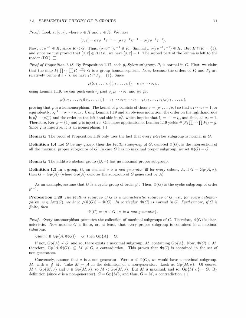
1.3. ELEMENTARY THEORY OF P -GROUPS 71
Proof . Look at [σ, τ ], where σ ∈ H and τ ∈ K. We have
[σ, τ ] = στσ−1τ−1 = (στσ−1)τ−1 = σ(τσ−1τ−1).
Now, στσ−1 ∈ K, since K C G. Thus, (στσ−1)τ−1 ∈ K. Similarly, σ(τσ−1τ−1) ∈ H. But H ∩K = 1,and since we just proved that [σ, τ ] ∈ H ∩K, we have [σ, τ ] = 1. The second part of the lemma is left to thereader (DX).
Proof of Proposition 1.18. By Proposition 1.17, each pj-Sylow subgroup Pj is normal in G. First, we claim
that the map P1
∏ · · ·∏Ptϕ−→ G is a group homomorphism. Now, because the orders of Pi and Pj are
relatively prime if i 6= j, we have Pi ∩ Pj = 1. Since
ϕ((σ1, . . . , σt)(τ1, . . . , τt)) = σ1τ1 · · ·σtτt,
using Lemma 1.19, we can push each τj past σj+1 · · ·σt, and we get
ϕ((σ1, . . . , σt)(τ1, . . . , τt)) = σ1 · · ·σtτ1 · · · τt = ϕ(σ1, . . . , σt)ϕ(τ1, . . . , τt),
proving that ϕ is a homomorphism. The kernel of ϕ consists of those σ = (σ1, . . . , σt) so that σ1 · · ·σt = 1, orequivalently, σ−1
t = σ1 · · ·σt−1. Using Lemma 1.19 and an obvious induction, the order on the righthand side
is pl11 · · · plt−1
t−1 and the order on the left hand side in pltt , which implies that l1 = · · · = lt, and thus, all σj = 1.Therefore, Ker ϕ = 1 and ϕ is injective. One more application of Lemma 1.19 yields #(P1
∏ · · ·∏Pt) = g.Since ϕ is injective, it is an isomorphism.
Remark: The proof of Proposition 1.18 only uses the fact that every p-Sylow subgroup is normal in G.
Definition 1.4 Let G be any group, then the Frattini subgroup of G, denoted Φ(G), is the intersection ofall the maximal proper subgroups of G. In case G has no maximal proper subgroup, we set Φ(G) = G.
Remark: The additive abelian group (Q,+) has no maximal proper subgroup.
Definition 1.5 In a group, G, an element σ is a non-generator iff for every subset, A, if G = GpA, σ,then G = GpA (where GpA denotes the subgroup of G generated by A).
As an example, assume that G is a cyclic group of order pr. Then, Φ(G) is the cyclic subgroup of orderpr−1.
Proposition 1.20 The Frattini subgroup of G is a characteristic subgroup of G, i.e., for every automor-phism, ϕ ∈ Aut(G), we have ϕ(Φ(G)) = Φ(G). In particular, Φ(G) is normal in G. Furthermore, if G isfinite, then
Φ(G) = σ ∈ G | σ is a non-generator.
Proof . Every automorphism permutes the collection of maximal subgroups of G. Therefore, Φ(G) is char-acteristic. Now assume G is finite, or, at least, that every proper subgroup is contained in a maximalsubgroup.
Claim: If GpA,Φ(G) = G, then GpA = G.
If not, GpA 6= G, and so, there exists a maximal subgroup, M , containing GpA. Now, Φ(G) ⊆ M ,therefore, GpA,Φ(G) ⊆ M 6= G, a contradiction. This proves that Φ(G) is contained in the set ofnon-generators.
Conversely, assume that σ is a non-generator. Were σ /∈ Φ(G), we would have a maximal subgroup,M , with σ /∈ M . Take M = A in the definition of a non-generator. Look at GpM,σ. Of course,M ⊆ GpM,σ and σ ∈ GpM,σ, so M < GpM,σ. But M is maximal, and so, GpM,σ = G. Bydefinition (since σ is a non-generator), G = GpM, and thus, G = M , a contradiction.

72 CHAPTER 1. GROUP THEORY
Definition 1.6 A group G is an elementary abelian p-group iff
(1) It is abelian, and
(2) For every σ ∈ G, we have σp = 1.
Remark: Any elementary abelian p-group is, in a natural way, a vector space over Fp. Conversely, forany vector space over the finite field Fp, its additive group is an elementary abelian p-group. Under thiscorrespondence, an endomorphism of G goes over to a linear map and an automorphism of G goes to aninvertible linear map. The group G is finite iff the corresponding vector space is finite dimensional.
(Given G, write the group operation additively. Thus, we have
p · σ = σ + · · ·+ σ︸ ︷︷ ︸p
= 0.
The finite field Fp acts on G as follows: If λ ∈ Fp = Z/pZ, i.e., λ ≡ 0, 1, . . . , p− 1 (mod p), we set
λ · σ = σ + · · ·+ σ︸ ︷︷ ︸λ (mod p) times
.
The reader should check that scalar multiplication is indeed well defined and that the facts asserted in theprevious remark are true (DX).)
Proposition 1.21 For any p-group, G, the quotient group, G/Φ(G), is an elementary abelian p-group.
Proof . Say H is a maximal subgroup of G. Since G has (N), the group, H, is normal in G and (G : H) = p.Therefore, G/H is cyclic of order p. Write σ for the image of σ in G/H. We know that (σ)p = 1. So, σp = 1,i.e., σp ∈ H. But H is arbitrary, and so,
σp ∈⋂
H maximal
H = Φ(G).
Now, G/H is abelian since G/H = Z/pZ. This implies that [G,G] ⊆ H (here [G,G] is the subgroup of Ggenerated by the commutators, called the commutator group of G; it is the smallest normal subgroup, K, ofG such that G/K is abelian). Since H is arbitrary, we get
[G,G] ⊆⋂
H maximal
H = Φ(G).
This shows that G/Φ(G) is abelian. As σp ∈ Φ(G), we get (σ)p = 1 in G/Φ(G), where σ is the image of σin G/Φ(G).
We now come to a famous theorem of Burnside.
Theorem 1.22 (Burnside Basis Theorem) Say G is a p-group and let d be the minimal number of elementsfound among all minimal generating sets for G. The following properties hold:
(1) Given any set of d elements in G, say σ1, . . . , σd, they generate G iff σ1, . . . , σd are a basis of G/Φ(G).
(2) More generally, any set of t elements σ1, . . . , σt in G generates G iff σ1, . . . , σt spans G/Φ(G). Hence,any set of generators of G possesses a subset of exactly d elements which generates G. The number dis the dimension of G/Φ(G) over Fp.

1.3. ELEMENTARY THEORY OF P -GROUPS 73
Proof . Everything follows from the statement: σ1, . . . , σt generate G iff σ1, . . . , σt generate G = G/Φ(G)(DX).
The implication (=⇒) is trivial and always true. Conversely, if σ1, . . . , σt generate G, then
G = Gpσ1, . . . , σt,Φ(G).
But then, as Φ(G) is the set of nongenerators, we have
G = Gpσ1, . . . , σt,Φ(G) = Gpσ1, . . . , σt,
as desired.
Let G be a group (possibly infinite). We set ∆(0)(G) = G, and ∆(1)(G) = [G,G] and, more generally
∆(j+1)(G) = [∆(j)(G),∆(j)(G)] = ∆(1)(∆(j)(G)).
Observe that ∆(1)(G) = [G,G] is the commutator group of G, and recall that for any normal subgroup, H,of G, we have ∆(1)(G) ⊆ H iff G/H is abelian. Moreover, for a simple nonabelian group, [G,G] = G.
Proposition 1.23 Suppose G is a group, then each ∆(j)(G) is a characteristic subgroup of G and eachgroup ∆(j)(G)/∆(j+1)(G) is abelian (j ≥ 0). If G has property (N), then ∆(1)(G) ⊆ Φ(G) < G (providedmaximal subgroups exist). If G is a p-group, then the chain
G ⊇ ∆(1)(G) ⊇ ∆(2)(G) ⊇ · · · ⊇ ∆(t)(G) ⊇ · · ·
is strictly descending and reaches 1 after finitely many steps.
Proof . The group ∆(1)(G) consists of products of the form
[σ1, τ1] · · · [σl, τl], l ≥ 1.
If ϕ ∈ Aut(G), then
ϕ([σ1, τ1] · · · [σl, τl]) = ϕ([σ1, τ1]) · · ·ϕ([σl, τl]),
and ϕ([σ, τ ]) = [ϕ(σ), ϕ(τ)], so ∆(1)(G) is characteristic. We prove that ∆(j)(G) is characteristic by inductionon j. The base case j = 1 has just been established. Look at ∆(j+1)(G). By the induction hypothesis, wehave ϕ(∆(j)(G)) = ∆(j)(G). Therefore, ϕ is an automorphism of ∆(j)(G). Yet, ∆(j+1)(G) = ∆(1)(∆(j)(G)),and we proved that ∆(1)(H) is characteristic for any group H (case j = 1). Now, G/∆(1)(G) is abelian forany group G, so ∆(j)(G)/∆(j+1)(G) = ∆(j)(G)/∆(1)(∆(j)(G)) is abelian.
Say G has (N) and possesses maximal subgroups. If H is a maximal subgroup of G we know that H CGand H has prime index. So, G/H is abelian, and thus, ∆(1)(G) ⊆ H. Since H is arbitrary, we deduce that
∆(1)(G) ⊆⋂
H maximal
H = Φ(G).
Now, assume that G is a p-group. Then, G has (N), and thus, ∆(1)(G) ⊆ Φ(G) < G. But ∆(1)(G) inturn is a p-group, so we can apply the argument to ∆(1)(G) and we get ∆(2)(G) < ∆(1)(G), etc.
Nomenclature.
(1) The group ∆(1)(G) is called the first derived group of G (or commutator group of G).
(2) The group ∆(j)(G) is the j-th derived group of G.

74 CHAPTER 1. GROUP THEORY
(3) The sequenceG = ∆(0)(G) ⊇ ∆(1)(G) ⊇ ∆(2)(G) ⊇ · · · ⊇ ∆(t)(G) ⊇ · · ·
is the derived series of G.
(4) The smallest t ≥ 0 for which ∆(t)(G) = 1 is the derived length of G and if ∆(t)(G) is never 1 (e.g.,in a nonabelian simple group) then the derived length is infinite. Write δ(G) for the derived length ofG.
Look at the derived series of G:
G = ∆(0)(G) ⊇ ∆(1)(G) ⊇ ∆(2)(G) ⊇ · · · ⊇ ∆(t)(G) ⊇ · · · .
Each quotient ∆(j)(G)/∆(j+1)(G) is abelian. Suppose G is finite, then ∆(j)(G)/∆(j+1)(G) is finite abelian.Interpolate between ∆(j)(G) and ∆(j+1)(G) a sequence of subgroups, necessarily normal, each maximal inthe previous one. If δ(G) < ∞, we get a composition series all of whose factors are cyclic of prime order.This proves half of the
Proposition 1.24 A necessary and sufficient condition that a finite group be solvable (in the sense of Galois)is that δ(G) <∞.
Proof . We need only prove: If G is (Galois) solvable, then δ(G) <∞. Say
G = G0 > G1 > G2 > · · · > Gt = 1
is a composition series with abelian factors. We have G1 < G and G/G1 is abelian. Therefore, by a previousremark, ∆(1)(G) ⊆ G1. Each quotient Gj/Gj+1 is abelian, so ∆(1)(Gj) ⊆ Gj+1 for all j. Now, ∆(1)(G) ⊆ G1
implies that ∆(1)(∆(1)(G)) ⊆ ∆(1)(G1), and so,
∆(2)(G) ⊆ ∆(1)(G1) ⊆ G2.
An easy induction yields ∆(r)(G) ⊆ Gr (DX). Therefore, ∆(t)(G) ⊆ 1, i.e., δ(G) ≤ t.Observe that we actually proved more: The derived length, δ(G), of a solvable finite group is less than
or equal to the length of any composition series for G.
Definition 1.7 An arbitrary group, G, is solvable iff δ(G) <∞.
Proposition 1.25 Say G is a p-group of order at least p2. Then, (G : ∆(1)(G)) ≥ p2.
Proof . We may assume that G is nonabelian, else ∆(1)(G) = 1 and so, (G : ∆(1)(G)) = #(G) ≥ p2. AsG is a p-group, if (G : ∆(1)(G)) < p2, then (G : ∆(1)(G)) = p. We know that ∆(1)(G) ⊆ Φ(G). Therefore,(G : Φ(G)) = p and the Burnside dimension of G (i.e. dimFp G/Φ(G)) is equal to 1. By the Burnside basistheorem, G is cyclic, so abelian, a contradiction.

1.4. GROUP EXTENSIONS 75
1.4 Group Extensions
Let G be a finite group and let
G = G0 > G1 > G2 > · · · > Gt = 1
be a composition series. We have the groups Gj/Gj+1 = Gj , the composition factors of the compositionseries.
Problem: Given the (ordered) sequence G0, G1, G2, . . . , Gt−1, try to reconstruct G.
Say H and K are two groups, G is a “big” group and H C G with G/H →K. Note, this is exactly thecase at the small end of a composition series. We haveGt−1 = Gt−1 = Gt−1/Gt. We also have Gt−1 C Gt−2, and the quotient is Gt−2, so we are in the abovesituation with H = Gt−1 = Gt−1, K = Gt−2, G = Gt−2, and G/H →K.
The above situation is a special case of an exact sequence. A diagram of groups and homomorphisms
0 −→ Hϕ−→ G ψ−→ K −→ 0,
where the map 0 −→ H is the inclusion of 1 into H and the map K −→ 0 is the surjection sendingevery element of K to 1 in the trivial group 1, is called a short exact sequence iff the kernel of everyhomomorphism is equal to the image of the previous homomorphism on its left. This means that
(1) Ker ϕ = 1, so ϕ is injective, and we identify H with a subgroup of G.
(2) H = Im ϕ = Ker ψ, so H is normal in G.
(3) Im ψ = K, so ψ is surjective. By the first homomorphism theorem, G/H →K.
(4) Properties (1), (2), (3) are equivalent to 0 −→ H −→ G −→ K −→ 0 is exact.
Going back to composition series, we have Gj+1 C Gj and Gj = Gj/Gj+1. So, a composition series isequivalent with a collection of short exact sequences
0 −→ Gt−1 −→ Gt−2 −→ Gt−2 −→ 0
0 −→ Gt−2 −→ Gt−3 −→ Gt−3 −→ 0
· · · · · · · · · · · · · · · · · · · · · · · · · · · · · · · · · · · ·0 −→ G1 −→ G −→ G0 −→ 0.
So our problem reduces to the problem of group extensions: Given H and K, groups, find (classify) allgroups, G, which can possibly fit into an exact sequence
0 −→ H −→ G −→ K −→ 0.
The problem is very hard when H is nonabelian.
Definition 1.8 If A,G are groups, a group, G, is an extension of G by A iff G fits into an exact sequence
(E) 0 −→ A −→ G −→ G −→ 0.
Two such extensions (E), (E′) are equivalent iff there exists a commutative diagram
(E) 0 // A // G //
ψ
G // 0
(E′) 0 // A // G′ // G // 0.

76 CHAPTER 1. GROUP THEORY
Remarks:
(1) The homomorphism, ψ, in the above diagram is an isomorphism of groups. So, the notion of equivalenceis indeed an equivalence relation (DX).
(2) Equivalence of group extensions is stronger than isomorphism of G with G′.(3) The group G in (E) should be considered a “fibre space” whose base is G and whose “fibre” is A.
As we remarked before, the theory is good only when A is abelian. From now on, we assume A is anabelian group.
Proposition 1.26 Say
(E) 0 −→ A −→ G −→ G −→ 0
is a group extension and A is abelian. Then, there exists a natural action of G on A; so, A is a G-module.Equivalent extensions give rise to the same action.
Proof . Denote the surjective homomorphism G −→ G in (E) by bar ( ). Pick ξ ∈ G and any a ∈ A. Thereexists x ∈ G with x = ξ. Consider xax−1. Since AC G, we have xax−1 ∈ A. If y ∈ G and if y = x = ξ, thenx = yα for some α ∈ A. Then,
xax−1 = yαaα−1y−1 = yay−1,
as A is abelian. Therefore, if we setξ · a = xax−1,
this is a well-defined map. The reader should check that it is an action (DX). Assume we have an equivalenceof extensions between (E) and (E′):
(E) 0 // A // G //
ψ
G // 0
(E′) 0 // A // G′ // G // 0.
Pick ξ ∈ G and any a ∈ A. Denote the E-action by · and the E′-action by · ·. Observe that
ξ · a = ψ(ξ · a) = ψ(xax−1) = ψ(x)ψ(a)ψ(x)−1 = ψ(x)aψ(x)−1,
since the left vertical arrow is the identity in the diagram, yet ψ(x) lifts ξ in G′, as the right vertical arrowis the identity in the diagram. However, by definition,
ξ · · a = ψ(x)aψ(x)−1,
so, ξ · · a = ξ · a for all a ∈ A.
The type of (E) is the structure of A as G-module, i.e., the action of G on A. We get a first invariant ofa group extension, its action (of G on A).
Fix the action of (E). Can we classify the extensions up to equivalence? Say we are given an extension
(E) 0 −→ A −→ G π−→ G −→ 0.
There is always a set-theoretic section s : G→ G, i.e., a set map, s, so that π(s(σ)) = σ for all σ ∈ G. Writeuσ for the s-lift of σ, i.e., s(σ) = uσ. So, π(uσ) = uσ = σ. As s is not necessarily a group homomorphism,what is the obstruction? Consider
uσuτ (uστ )−1 = f(σ, τ). (∗)

1.4. GROUP EXTENSIONS 77
Note that f(σ, τ) = 1 iff s : σ 7→ uσ is a group homomorphism. If we apply the homomorphism bar to (∗),we get f(σ, τ) = 1, and so, f(σ, τ) ∈ A. Observe that f is a functionf : G
∏G → A. Given x ∈ G, look at x. We know that x = σ ∈ G. If we apply bar to xu−1
σ , we get 1,
because u−1σ = σ−1 and x = σ. So, we have xu−1
σ ∈ A, which yields x = auσ, for some a ∈ A.
Observe that:
(1) Each x determines uniquely a representation x = auσ, with a ∈ A and σ ∈ G.
(2) The map A∏G −→ G (where A
∏G is the product of A and G as sets) via
(a, σ) 7→ auσ
is a bijection of sets (an isomorphism in the category of sets).
(3) G (as a set) is just A∏G (product in the category of sets).2
Can we recover the group multiplication of G? We have
(auσ)(buτ ) = a(uσb)uτ
= a(uσbu−1σ )uσuτ
= a(σ · b)uσuτ= a(σ · b)f(σ, τ)uστ
= cuστ ,
where c = a(σ · b)f(σ, τ), and c ∈ A. Therefore, knowledge of the action and f(σ, τ) gives us knowledge ofthe group multiplication.
Thus, it is natural to try to go backwards and make G from the groups A and G, the action of G on A,and f . It is customary to use an additive notation for the group operation in A, since A is abelian. Theunderlying set of the group G is
A∏
G = 〈a, σ〉 | a ∈ A, σ ∈ G.
Multiplication is given by
〈a, σ〉〈b, τ〉 = 〈a+ σ · b+ f(σ, τ), στ〉. (†)
However, the multiplication defined by (†) is supposed to make G into a group, and this imposes certainconditions on f . First, we deal with associativity. For this, we go back to the original G where we have theassociative law:
(auσ)((buτ )(cuρ)) = ((auσ)(buτ ))(cuρ).
Expanding the left hand side, we get
(auσ)((buτ )(cuρ)) = (auσ)(b(τ · c)f(τ, ρ)uτρ)
= (aσ · (b(τ · c)f(τ, ρ))f(σ, τρ)uσ(τρ)
= a(σ · b)(στ · c)(σ · f(τ, ρ))f(σ, τρ)uσ(τρ).
Expanding the righthand side, we get
((auσ)(buτ ))(cuρ) = a(σ · b)f(σ, τ)uστ )(cuρ)
= a(σ · b)f(σ, τ)(στ · c)f(στ, ρ)u(στ)ρ.
2In (2) and (3) we give a foretaste of the language of categories to be introduced in Section 1.7.

78 CHAPTER 1. GROUP THEORY
Thus, the associative law becomes (writing RHS = LHS)
f(σ, τ)(στ · c)f(στ, ρ) = (στ · c)(σ · f(τ, ρ))f(σ, τρ).
Now, all the above terms are in A, and since A is abelian, we can permute terms and perform cancellations,and we get
f(σ, τ)f(στ, ρ) = (σ · f(τ, ρ))f(σ, τρ). (††)This identity is equivalent to the associativity law in G.
Nomenclature: A function from G∏G to A is called a 2-cochain on G with values in A. Any 2-cochain
satisfying (††) is called a 2-cocycle with coefficients in A.
Therefore, (†) is an associative multiplication in A∏G iff f is a 2-cocycle with values in A.
Does A∏G with multiplication (†) have an identity?
The original group, G, has identity 1 and we have 1 = u−11 u1, where u1 ∈ A, and so, u−1
1 ∈ A. For allb ∈ A and all τ ∈ G, we have
(u−11 u1)(buτ ) = buτ ,
which yieldsu−1
1 (1 · b)f(1, τ)uτ = u−11 bf(1, τ)uτ = buτ .
Since A is abelian, we getf(1, τ) = u1,
which shows that f(1, τ) is independent of τ . In particular, u1 = f(1, 1).
Question: Is (††) sufficient to imply that f(1, τ) = f(1, 1) for all τ ∈ G?
In (††), take σ = 1. We getf(1, τ)f(τ, ρ) = f(τ, ρ)f(1, τρ).
Again, since A is abelian, we deduce that f(1, τ) = f(1, τρ). If we take τ = 1, we get f(1, 1) = f(1, ρ), forall ρ.
Therefore, (††) is sufficient and A∏G has an identity 1 = 〈f(1, 1)−1, 1〉, or in additive notation (since
A is abelian),
1 = 〈−f(1, 1), 1〉. (∗)
Finally, what about inverses? Once again, go back to our original G.
We have (auσ)−1 = u−1σ a−1. Now,
u−1σ = (uσ)−1 = σ−1 = uσ−1 .
Therefore, there is some α ∈ A so that u−1σ = αuσ−1 . By multiplying on the right by uσ, we get
1 = αuσ−1uσ = αf(σ−1, σ)uσσ−1 = αf(σ−1, σ)u1 = αf(σ−1, σ)f(1, 1),
since u1 = f(1, 1). So, α = f(1, 1)−1f(σ−1, σ)−1. Consequently, we get
(auσ)−1 = u−1σ a−1
= αuσ−1a−1
= α(uσ−1a−1u−1σ−1)uσ−1
= α(σ−1 · a−1)uσ−1
= f(1, 1)−1f(σ−1, σ)−1(σ−1 · a−1)uσ−1
= f(1, 1)−1f(σ−1, σ)−1(σ−1 · a)−1uσ−1
= ((σ−1 · a)f(σ−1, σ)f(1, 1))−1uσ−1 .

1.4. GROUP EXTENSIONS 79
Therefore, in A∏G (switching to additive notation since A is abelian), inverses are given by
〈a, σ〉−1 = 〈−σ−1 · a− f(σ−1, σ)− f(1, 1), σ−1〉. (∗∗)
We find that A∏G can be made into a group via (†), provided f(σ, τ) satisfies (††). The formulae (∗)
and (∗∗) give the unit element and inverses, respectively. For temporary notation, let us write (A∏G; f)
for this group. Also, since A is abelian, let us rewrite (††) in additive notation, since this will be moreconvenient later on:
σ · f(τ, ρ) + f(σ, τρ) = f(στ, ρ) + f(σ, τ). (††)
Go back to the original group, G, and its set-theoretic section s : G→ G (with s(σ) = uσ). We might havechosen another set-theoretic section, t : G→ G, namely, t(σ) = vσ. We get a 2-cocycle g(σ, τ) = vσvτ (vστ )−1,i.e., vσvτ = g(σ, τ)vστ .
What is the relation between f and g?
We know that vσ = σ = uσ, which implies that there is some k(σ) ∈ A with vσ = k(σ)uσ. Then, we have
vσvτ = g(σ, τ)vστ = g(σ, τ)k(στ)uστ ,
and also
vσvτ = k(σ)uσk(τ)uτ = k(σ)(σ · k(τ))uσuτ = k(σ)(σ · k(τ))f(σ, τ)uστ .
By equating these expressions, we get
g(σ, τ)k(στ) = k(σ)(σ · k(τ))f(σ, τ).
But A is abelian, so we can write the above
g(σ, τ)− f(σ, τ) = σ · k(τ)− k(στ) + k(σ). (∗)
Observe that k : G → A is a function of one variable on G. We call k a 1-cochain on G with values in A.For a 1-cochain, define a corresponding 2-cochain, called its coboundary , δk, by
(δk)(σ, τ) = σ · k(τ)− k(στ) + k(σ).
Remarks:
(1) Every coboundary of a 1-cochain is automatically a 2-cocycle (DX).
(2) Cocycles form a group under addition of functions denoted by Z2(G,A). The special 2-cocycles whichare coboundaries (of 1-cochains) form a group (DX) denoted by B2(G,A). Item (1) says that B2(G,A)is a subgroup of Z2(G,A).
(3) The quotient group, Z2(G,A)/B2(G,A), denoted H2(G,A), is the second cohomology group of G withcoefficients in A.
(4) Equation (∗) above says: If we change the choice of section from s to t, the corresponding cocycles, fand g, are cohomologous, i.e., g − f = δk, i.e., the image of f in H2(G,A) is the same as the image ofg in H2(G,A). Thus, it is the cohomology class of f which is determined by (E).

80 CHAPTER 1. GROUP THEORY
Now, make (A∏G; f). Then, we can map A into (A
∏G; f) via
a 7→ 〈a− f(1, 1), 1〉.
Claim. The set 〈a − f(1, 1), 1〉 | a ∈ A is a subgroup of (A∏G; f). In fact, it is a normal subgroup and
the quotient is G.
Proof . We have
〈a− f(1, 1), 1〉〈b− f(1, 1), 1〉 = 〈a− f(1, 1) + b− f(1, 1) + f(1, 1), 1〉 = 〈a+ b− f(1, 1), 1〉,
and thus, the map λ : a 7→ 〈a− f(1, 1), 1〉 is a group homomorphism. We leave the rest as a (DX).
Say f − g = δk, i.e., f and g are cohomologous, and make (A∏G; f) and (A
∏G; g). Consider the map
θ : (A∏G; f)→ (A
∏G; g) given by
θ : 〈a, σ〉 7→ 〈a+ k(σ), σ〉.We claim that θ is a homomorphism. Since
〈a, σ〉〈b, τ〉 = 〈a+ σ · b+ f(σ, τ), στ〉,
we haveθ(〈a, σ〉〈b, τ〉) = 〈a+ σ · b+ f(σ, τ) + k(στ), στ〉.
We also have
θ(〈a, σ〉)θ(〈b, τ〉) = 〈a+ k(σ), σ〉〈b+ k(τ), τ〉)= 〈a+ k(σ) + σ · b+ σ · k(τ) + g(σ, τ), στ〉).
In order for θ to be a homomorphism, we need
k(σ) + σ · k(τ) + g(σ, τ) = f(σ, τ) + k(στ),
that is, f − g = δk. Consequently, θ is a homomorphism, in fact, an isomorphism. Moreover, (A∏G; f) and
(A∏G; g) fit into two extensions and we have the following diagram:
(E)f 0 // A // (A∏G; f) //
θ
G // 0
(E′)g 0 // A // (A∏G; g) // G // 0.
The rightmost rectangle commutes, but we need to check that the leftmost rectangle commutes. Going overhorizontally and down from (A
∏G; f), for any a ∈ A, we have
a 7→ 〈a− f(1, 1), 1〉 7→ 〈a− f(1, 1) + k(1), 1〉,
and going horizontally from the lower A, we have
a 7→ 〈a− g(1, 1), 1〉.
For the rectangle to commute, we need: g(1, 1) = f(1, 1)− k(1). However,f(σ, τ) = g(σ, τ) + δk(σ, τ) and δk(σ, τ) = σ · k(τ)− k(στ) + k(σ). If we set σ = τ = 1, we get
δk(1, 1) = k(1)− k(1) + k(1) = k(1),
and it follows that g(1, 1) = f(1, 1)− k(1), as desired.

1.4. GROUP EXTENSIONS 81
Hence, cohomologous 2-cocycles give rise to equivalent group extensions (the action is fixed). Conversely,we now show that equivalent group extensions give rise to cohomologous 2-cocycles. Say
(E) 0 // A // G //
ψ
G // 0
(E′) 0 // A // G′ // G // 0.
is an equivalence of extensions (i.e., the diagram commutes). We know, up to the notion of being cohomol-ogous, that we may adjust both cocycles f and g associated with (E) and (E′) by choice of sections. Inboth cases, take u1 = 0 (since we are using additive notation). Therefore, f(1, 1) = g(1, 1) = 0. From thecommutativity of the diagram, ψ must be of the form
ψ〈a, σ〉 = 〈ϕ(a, σ), σ〉
for some function ϕ : A∏G → A. By the above choice, the maps A −→ G and A −→ G′ are given by
a 7→ 〈a, 1〉 in both cases. Therefore,ψ(a, 1) = 〈ϕ(a, 1), 1) = (a, 1), and so,
ϕ(a, 1) = a, for all a ∈ A.
Since ψ is a homomorphism, we have
ψ(〈a, σ〉〈b, τ〉) = ψ(〈a, σ〉)ψ(〈b, τ〉),
and this yields an identity relating f , g and ϕ. The left hand side of the above equation is equal to
ψ(〈a+ σ · b+ f(σ, τ), στ〉) = 〈ϕ(a+ σ · b+ f(σ, τ), στ〉), στ〉,
and the righthand side is equal to
〈ϕ(a, σ), σ〉〈ϕ(b, τ), τ〉 = 〈ϕ(a, σ) + σ · ϕ(b, τ) + g(σ, τ), στ〉,
and by equating them, we get
ϕ(a+ σ · b+ f(σ, τ), στ〉) = ϕ(a, σ) + σ · ϕ(b, τ) + g(σ, τ). (†††)
By taking τ = 1 (using the fact that ϕ(b, 1) = b), we get
ϕ(a+ σ · b+ f(σ, 1), σ〉) = ϕ(a, σ) + σ · b+ g(σ, 1). (∗∗∗)
Now, (††) can be written as
σ · f(τ, ρ)− f(στ, ρ) + f(σ, τρ)− f(σ, τ) = 0.
If we take ρ = 1, we getσ · f(τ, 1)− f(στ, 1) + f(σ, τ)− f(σ, τ) = 0.
which yieldsσ · f(τ, 1) = f(στ, 1).
If we take τ = 1, we get σ · f(1, 1) = f(σ, 1), but f(1, 1) = 0, and so,
f(σ, 1) = 0.
Consequently, (∗∗∗) yieldsϕ(a+ σ · b, σ) = ϕ(a, σ) + σ · b.

82 CHAPTER 1. GROUP THEORY
Writing b = σ−1 · c, we getϕ(a+ c, σ) = ϕ(a, σ) + c, for all a, c ∈ A.
In particular, when a = 0, we get ϕ(c, σ) = ϕ(0, σ)+c. Let ϕ(0, σ) = k(σ). Now, if we use ϕ(a, σ) = ϕ(0, σ)+ain (†††), we get
a+ σ · b+ f(σ, τ) + k(στ) = a+ k(σ) + σ · (b+ k(τ)) + g(σ, τ),
which yieldsf(σ, τ) + k(στ) = g(σ, τ) + k(σ) + σ · k(τ),
that is, f − g = δk. Hence, we have proved almost all of the following fundamental theorem:
Theorem 1.27 If G and A are groups and A is abelian, then each group extension
(E) 0 −→ A −→ G π−→ G −→ 0
makes A into a G-module; the G-module structure is the type of (E) and equivalent extensions have the sametype. For a given type, the equivalence classes of extensions of G by A are in one-to-one correspondencewith H2(G,A), the second cohomology group of G with coefficients in A. Hence, the distinct extensions ofG by A (up to equivalence) are classified by the pairs (type(E), χ(E)), where χ(E) is the cohomology classin H2(G,A) corresponding to (E). In this correspondence, central extensions correspond to G-modules, A,with trivial action ((E) is central iff A ⊆ Z(G)). An extension of any type splits iff χ(E) = 0 in H2(G,A).((E) is split iff there is a group homomorphism s : G→ G so that π s = id).
Proof . We just have to prove the last two facts. Note that the type of extension is trivial iff
(∀σ ∈ G)(∀a ∈ A)(σ · a = a)
iff(∀x ∈ G)(∀a ∈ A)(x−1ax = a)
iff(∀x ∈ G)(∀a ∈ A)([x, a] = 1)
iff A ⊆ Z(G).
Finally, the cohomology is trivial iff every cocycle is a coboundary iff every cocycle is cohomologous to0 iff in (E) there is a map σ 7→ uσ with f(σ, τ) = 0. Such a map is a homomorphism. Thus, χ(E) = 0 inH2(G,A) iff (E) has a splitting.
Examples. (I) Find all extensions
0 −→ Z −→ G −→ Z/2Z −→ 0.
There are several cases to consider depending on the type and the cohomology class of the extension.
(a) Trivial type (the action of Z/2Z on Z is trivial).
(a1) Split extension. We get G → Z∏
(Z/2Z).
(a2) Nonsplit extensions. In this case, we have to compute H2(Z/2Z,Z) (trivial action). We know fromprevious work that (up to cohomology) we can restrict ourselves to normalized cochains, f(σ, τ), i.e., cochainssuch that
f(σ, 1) = f(1, σ) = 0.
Elements in Z/2Z are ±1. We need to know what f(−1,−1) is. The reader should check that the co-cycle condition, δf = 0, gives no condition on the integer f(−1,−1), and thus, we have an isomorphismZ2(Z/2Z,Z) ∼= Z.

1.4. GROUP EXTENSIONS 83
What about coboundaries: f = δk? Such k’s are also normalized, and so, k(1) = 0. We have k(−1) = b,for any b ∈ Z. Since
δk(σ, τ) = σ · k(τ)− k(στ) + k(σ),
using the fact that the action is trivial and that k(1) = 0, we get
δk(−1,−1) = (−1) · k(−1)− k(1) + k(−1) = k(−1) + k(−1) = 2b.
So, we can adjust f , up to parity by coboundaries, and H2(Z/2Z,Z) ∼= Z/2Z. Consequently, we have exactlyone nonsplit, trivial-type extension
G = (n,±1) | n ∈ Z.The group operation is given by
(n,±1)(m, 1) = (n+m,±1)
(n, 1)(m,±1) = (n+m,±1)
(n,−1)(m,−1) = (n+m+ 1, 1),
where in this last equation, we assumed without loss of generality that f(−1,−1) = 1.
(b) Nontrivial type. We need a nontrivial map Z/2Z −→ Aut(Z). Since Z is generated by 1 and −1,there is only one nontrivial action:
(−1) · n = −n.(Recall that 1 · n = n, always).
(b1) The split, nontrivial type extension. In this case
G = (n, σ) | n ∈ Z, σ ∈ Z/2Z,
with multiplication given by
(n, σ)(m, τ) = (n+ σ ·m,στ).
Now, consider the map
(n, σ) 7→(σ n0 1
).
Observe that matrix multiplication yields
(σ n0 1
)(τ m0 1
)=
(στ n+ σ ·m0 1
).
Therefore, G is isomorphic to the group of matrices
(σ n0 1
)
under matrix product. This is a nonabelian group, it is infinite and we claim that G is solvable with δ(G) = 2.
Indeed, we have G/Z ∼= Z/2Z, an abelian group, and so ∆(1)(G) ⊆ Z. So,∆(2)(G) ⊆ ∆(1)(Z) = 0, and we conclude that δ(G) = 2.
(b2) Nonsplit, nontrivial type extension. We need to figure out what the cocycles are in order to computeH2(Z/2Z,Z). By the same reasoning as before, we need to know what is f(−1,−1). We know that δf(σ, τ) =0. So, we have
σ · f(τ, ρ)− f(στ, ρ) + f(σ, τρ)− f(σ, τ) = 0.

84 CHAPTER 1. GROUP THEORY
Let τ = ρ = −1 in the above equation. We get
σ · f(−1,−1)− f(−σ,−1) + f(σ, 1)− f(σ,−1) = σ · f(−1,−1)− f(−σ,−1)− f(σ,−1) = 0,
since f(σ, 1) = 0. If we let σ = −1, since f(1,−1) = 0, we get
−f(−1,−1)− f(−1,−1) = 0,
and so, 2f(−1,−1) = 0. Since f(−1,−1) ∈ Z, we get f(−1,−1) = 0. Therefore, f ≡ 0 and the cohomologyis trivial: H2(Z/2Z,Z) = (0) (for nontrivial action).
As a conclusion, there exist three extension classes and three distinct groups, two of them abelian, thethird solvable and faithfully representable by matrices.
(II) Let V be a finite dimensional vector space and consider V + as additive group. Let G = GL(V ) andlet the action of G on V be the natural one (i.e, for any ϕ ∈ GL(V ) and any v ∈ V , ϕ · v = ϕ(v)). We havethe split extension
0→ V → G GL(V )→ 0.
The group, G, in the above exact sequence is the affine group of V .
(III) Again, we restrict ourselves to split extensions. Let A be any abelian group and let n ∈ N. Thegroup
A∏
A∏· · ·∏
A︸ ︷︷ ︸
n
is acted on by the symmetric group, Sn, simply by permuting the factors. We have a split extension
0→ A∏
A∏· · ·∏
A︸ ︷︷ ︸
n
→ G Sn → 0.
The group, G, is called the wreath product of A by Sn and is denoted A oSn. We denote the split extensionof a given type of G by A by A \\// G (note that this notation does not refer to the action).
Here are some useful facts on cohomology:
(1) If G is arbitrary and A is n-torsion, which means that nA = 0, then H2(G,A) is n-torsion.
(2) If G is a finite group, say #(G) = g and A is arbitrary, then H2(G,A) is g-torsion (this is not trivialto prove!).
(3) Suppose that A is n-torsion and G is finite, with #(G) = g, and suppose that (g, n) = 1. Then,H2(G,A) = (0). (This is a clear consequence of (1) and (2).)
(4) Suppose that G is finite. We can define a homomorphism (of G-modules) A −→ A, called the G-normand denoted NG (we will usually drop the subscript G), defined by
NG(a) =∑
σ∈Gσ · a.
Moreover, assume that G is a finite cyclic group. Then, for any A, there is an isomorphism
AG/NA ∼= H2(G,A),
whereAG = a ∈ A | σ · a = a, for all σ ∈ G.

1.4. GROUP EXTENSIONS 85
Here is an example of how to use the above facts.
(IV) Find all the groups of order pq (with p, q prime and 0 < p < q).
We know that the q-Sylow subgroup is normal, namely, it is Z/qZ = AC G, andG = G/A = Z/pZ. Therefore, whatever G is, it fits in the group extension
0 −→ Z/qZ −→ G −→ Z/pZ −→ 0.
By (3), since (p, q) = 1, we have H2(G,A) = (0). So, we only have split extensions. What is Aut(Z/qZ)?Clearly, it is Z/(q − 1)Z. So, we have to consider the homomorphisms
Z/pZ −→ Aut(Z/qZ) = Z/(q − 1)Z. (∗)
If (∗) is non-trivial, then p | (q− 1), i.e., q ≡ 1 (mod p). So, if q 6≡ 1 (mod p), then we have trivial action andwe find that
G ∼= (Z/qZ)∏
(Z/qZ) ∼= Z/pqZ.
If q ≡ 1 (mod p), we also can have trivial action, and we get Z/pqZ, again. So, we now consider nontrivialactions. The unique cyclic group of order p in Z/(q − 1)Z is generated by λ q−1
p , where λ = 1, 2, . . . , p − 1.
If we send 1 ∈ Z/pZ to λ q−1p , the corresponding action is
n 7→ nλq − 1
p(mod q).
Thus, there are p− 1 nontrivial (split) group extensions, (Eλ), with central groups
Gλ = (n, ζm) | 0 ≤ m ≤ p− 1
(here the elements of Z/pZ are 1, ζ, ζ2, . . . , ζp−1) and multiplication given by
(n, ζm)(r, ζs) =
((n+ rmλ
q − 1
p, ζm+s
).
Consider the map Gλ −→ G1 given by
(n, ζm) 7→ (m, ζλm).
This is a group isomorphism. So, here we have all inequivalent extensions, (Eλ), with p−1 different actions,yet the groups Gλ are mutually isomorphic. Thus, G1 and Z/pqZ are the two groups of order pq whenq ≡ 1 (mod p).
The second cohomology group, H2(G,A), has appeared naturally in the solution to the group extensionproblem. Consequently, it is natural at this stage to define cohomology groups in general.
The set up is: We have a group, G, and a G-action, G∏A −→ A, where A is an abelian group. For
every n ∈ N, we define
Cn(G,A) = f : G∏· · ·∏
G︸ ︷︷ ︸
n
→ A,
where G∏· · ·∏
G︸ ︷︷ ︸
n
is the product of G with itself n times (in the category of sets). By convention, when
n = 0, this set product is the one point set, ∗. The set Cn(G,A) is an abelian group under additionof functions (e.g , f + g is the function defined by (f + g)(x) = f(x) + g(x) for all x ∈ G). The group

86 CHAPTER 1. GROUP THEORY
Cn(G,A) is called the group of n-cochains of G with coefficients in A. We define the coboundary map,δn : Cn(G,A)→ Cn+1(G,A), for every n ≥ 0, by the formula:
(δnf)(σ1, . . . , σn+1) = σ1 · f(σ2, . . . , σn+1) +
n∑
j=1
(−1)jf(σ1, . . . , σj−1, σjσj+1, σj+2, . . . , σn+1)
+ (−1)n+1f(σ1, . . . , σn),
for all f ∈ Cn(G,A) and all σ1, . . . , σn+1 ∈ G.
(1) Check (DX): For all n ≥ 0,δn(δn−1f) ≡ 0.
(By convention, δ−1 = 0).
(2) Set Zn(G,A) = Ker δn, a subgroup of Cn(G,A), the group of n-cocycles of G with coefficients inA. We also let Bn(G,A) = Im δn−1, a subgroup of Cn(G,A), the group of n-coboundaries of G withcoefficients in A. Observe that since δ−1 = 0, we have B0(G,A) = (0). Furthermore, (1) implies thatBn(G,A) ⊆ Zn(G,A), for all n ≥ 0.
(3) Set Hn(G,A) = Zn(G,A)/Bn(G,A); this is the nth cohomology group of G with coefficients in A.
Examples. (i) Case n = 0: Then, B0 = (0). The functions, f , in C0(G,A) are in one-to-one correspondencewith the elements f(∗) of A, and so, C0(G,A) = A. Note that for any σ ∈ G, if f ∈ C0(G,A) correspondsto the element a in A, we have
(δ0f)(σ) = σ · f(∗)− f(∗) = σ · a− a.
Thus,Z0(G,A) = a ∈ A | δ0(a) = 0 = a ∈ A | σ · a = a, for all σ ∈ G = AG.
So, we also have H0(G,A) = AG.
(ii) Case n = 1: Then, C1(G,A) is the set of all functions f : G→ A. For anyf ∈ C1(G,A), we have
(δ1f)(σ, τ) = σ · f(τ)− f(στ) + f(σ).
It follows that
Z1(G,A) = f ∈ C1(G,A) | δ1f = 0 = f ∈ C1(G,A) | f(στ) = σ · f(τ) + f(σ).
This is the set of crossed (or twisted) homomorphisms from G to A.
Remark: If A has trivial G-action, then Z1(G,A) = HomGr(G,A).
We have B1(G,A) = Im δ0 = all functions, g, so that g(σ) = (δ0(a))(σ) = σ · a − a, for some a ∈ A.Such objects are twisted homomorphisms, called principal (or inner) twisted homomorphisms.
Remark: If A has trivial G-action, then B1(G,A) = (0). So, H1(G,A) is the quotient of the twistedhomomorphisms modulo the principal twisted homomorphisms if the action is nontrivial, and H1(G,A) =HomGr(G,A) if the action is trivial.
(iii) Case n = 2: We have already encountered this case in dealing with group extensions. We contentourselves with computing δ2. Since C2(G,A) = f : G
∏G→ A, we have
(δ2f)(σ, τ, ρ) = σ · f(τ, ρ)− f(στ, ρ) + f(σ, τρ)− f(σ, τ).

1.4. GROUP EXTENSIONS 87
We note that Z2(G,A) gives us back the group of “old” 2-cocycles, B2(G,A) gives us back the group of“old” 2-coboundaries, and H2(G,A) is in one-to-one correspondence with the equivalence classes of groupextensions of a fixed type.
Remark: Given a group, G, Eilenberg and Mac Lane (1940’s) constructed a topological space, K(G, 1),unique up to homotopy type, with the following properties:
πn(K(G, 1)) =
G if n = 1(0) if n 6= 1.
Fact: If we compute the integral cohomology of K(G, 1), denoted Hn(K(G, 1),Z), we get
Hn(K(G, 1),Z) ∼= Hn(G,Z).
Here, the G-action on Z is trivial.

88 CHAPTER 1. GROUP THEORY
1.5 Solvable and Nilpotent Groups
Given a group, G, its derived series,
G = ∆(0)(G) ⊇ ∆(1)(G) ⊇ ∆(2)(G) ⊇ · · · ⊇ ∆(t)(G) ⊇ · · · ,
may decrease very quickly, and even though the solvable groups (those for which the derived series reaches1 after finitely many steps, i.e., those for which δ(G) is finite) are not as “wild” as groups for whichδ(G) = ∞, it desirable to delineate families of groups with an even “nicer” behavior. One way of doingso is to define descending (or ascending) chains that do not decrease (or increase) too quickly and then toinvestigate groups whose chains are finite. The collection of nilpotent groups is such a family of groups, and,moreover, nilpotent groups tend to show up as fundamental groups of spaces arising naturally in geometry.Every nilpotent group is solvable and solvability is inherited by subgroups and quotient groups, as shown inthe following proposition:
Proposition 1.28 If G is a group and G is solvable, then for every subgroup, H, of G, the group, H, issolvable. Moreover, if H is normal in G, then G/H is solvable. In fact, for both groups, δ(either) ≤ δ(G).Conversely, say G possesses a normal subgroup, H, so that both H and G/H are solvable. Then, G issolvable. In fact, δ(G) ≤ δ(H) + δ(G/H).
Proof . Let G be solvable. Then, H ⊆ G implies ∆(1)(H) ⊆ ∆(1)(G); therefore (by induction),
∆(j)(H) ⊆ ∆(j)(G),
and we deduce that δ(H) ≤ δ(G). Consider G = G/H when H C G. Then, [x, y] = [x, y] and this implies
∆(1)(G) = ∆(1)(G). Hence (by induction),
∆(j)(G) = ∆(j)(G).
Therefore, δ(G) ≤ δ(G).
Conversely, assume that H and G/H are solvable (with H C G). We have ∆(j)(G) = ∆(j)(G) and if
j ≥ δ(G), then ∆(j)(G) = 1, which implies that ∆(j)(G) ⊆ H. So, ∆(k+j)(G) ⊆ ∆(k)(H), and the latteris 1 if k = δ(H). Therefore,
∆(δ(G)+δ(H))(G) = 1,and so, δ(G) ≤ δ(H) + δ(G/H).
Proposition 1.29 Let (P) be some property of finite groups. Assume that (P) satisfies:
(a) The trivial group has (P), every cyclic group of prime order has (P).
(b) Suppose G has (P), then H CG implies H and G/H have (P).
(c) If G has (P) (with G 6= 1), then G is not simple unless G is cyclic of prime order.
Then, when G has (P), the group G is solvable.
Proof . We proceed by induction on #(G). The case G = 1 is trivial, by (a) (nothing to check). Assumethat the proposition holds for all G with #(G) ≤ n, and assume #(G) = n+ 1. If n+ 1 is prime, then G iscyclic of prime order, which implies that it is solvable. Thus, we may assume that n + 1 is not prime andthat G has (P). By (c), the group G has some nontrivial normal subgroup, H. By (b), both H and G/Hhave (P), and the induction hypothesis implies that both H and G/H are solvable. Proposition 1.28 impliesthat G is solvable.
Corollary 1.30 (Burnside, Feit & Thompson) Every group G, of order paqb or odd order is solvable.

1.5. SOLVABLE AND NILPOTENT GROUPS 89
Remark: Corollary 1.30 is not really proved. It depends on establishing (c) for the two properties: paqb,odd order. As remarked just before Proposition 1.10, this is not easy.
Definition 1.9 Let G be any group. The lower central series (LCS) of G is the descending chain ofsubgroups
G = Γ0 ⊇ Γ1 ⊇ · · · ⊇ Γd ⊇ · · · ,where Γj+1 = [G,Γj ]. The upper central series (UCS) of G is the ascending chain of subgroups
1 = Z0 ⊆ Z1 ⊆ Z2 ⊆ · · · ⊆ Zd ⊆ · · · ,where Zj = the inverse image in G of Z(G/Zj−1).
Remarks:
(1) Γ1(G) = [G,Γ0] = [G,G] = ∆(1)(G), and
Γ2(G) = [G,Γ1] = [G,∆(1)(G)] ⊇ [∆(1)(G),∆(1)(G)] = ∆(2)(G),
and so, Γ2(G) ⊇ ∆(2)(G). The reader should check (DX) that Γd(G) ⊇ ∆(d)(G), for all d ≥ 0.
(2) Z1(G) = inverse image in G of Z(G/Z0) = inverse image of Z(G), so Z1(G) = Z(G).
(3) If for some j, the equality Γj(G) = Γj+1(G) holds, then Γj(G) = Γd(G), for all d ≥ j. The lowercentral series strictly descends until the first repetition.
(4) Similarly, if for some j, the equality Zj(G) = Zj+1(G) holds, then Zj(G) = Zd(G), for all d ≥ j. Theupper central series strictly ascends until the first repetition.
Proposition 1.31 Suppose the lower central series of G reaches 1 after r steps. Then, for every j ≤ r,we have Γr−j ⊆ Zj. Consequently, the upper central series reaches G after r steps. Conversely, suppose thatthe upper central series reaches G after r steps. Then, for every j ≤ r, we have Γj ⊆ Zr−j. Consequently,the lower central series reaches 1 after r steps.
Proof . By induction on j. For j = 0, we have Γr = Γr−0, and by hypothesis, Γr = 1 and Z0 = 1, so thebasis of the induction holds. Before we do the induction step, let us also consider the case j = 1. We needto show that Γr−1 ⊆ Z1 = Z(G). But Γr = 1, yet Γr = [G,Γr−1]. This means that for all σ ∈ G and allτ ∈ Γn−1, we have [σ, τ ] ∈ Γr = 1. Thus, τ commutes with all σ ∈ G, and so, τ ∈ Z(G) = Z1. Let us nowassume our statement, Γr−j ⊆ Zj , for some j, and look at the case j + 1. Now, Γr−j = [G,Γr−j−1]. By theinduction hypothesis,
[G,Γr−j−1] ⊆ Zj .Consider the map G −→ G/Zj = G. Then,
[G,Γr−j−1] = 1 in G.
Therefore, Γr−j−1 is contained in the inverse image of Z(G) = Z(G/Zj) = Zj+1, concluding the inductionstep.
For the converse, again, use induction on j. When j = 0, we have Γ0 = G and Zr = Zr−0 = G, byhypothesis, and the basis of the induction holds. Assume that Γj ⊆ Zr−j for some j, and consider the casej + 1. We have
Γj+1 = [G,Γj ] ⊆ [G,Zr−j ],
by the induction hypothesis. Look at the map G −→ G/Zr−j−1 = G. We have
Γj+1 ⊆ [G,Zr−j ].
But, by definition, Zr−j = Z(G). Thus, [G,Zr−j ] = 1 in G. Therefore,Γj+1 ⊆ Ker (G −→ G) = Zr−j−1.
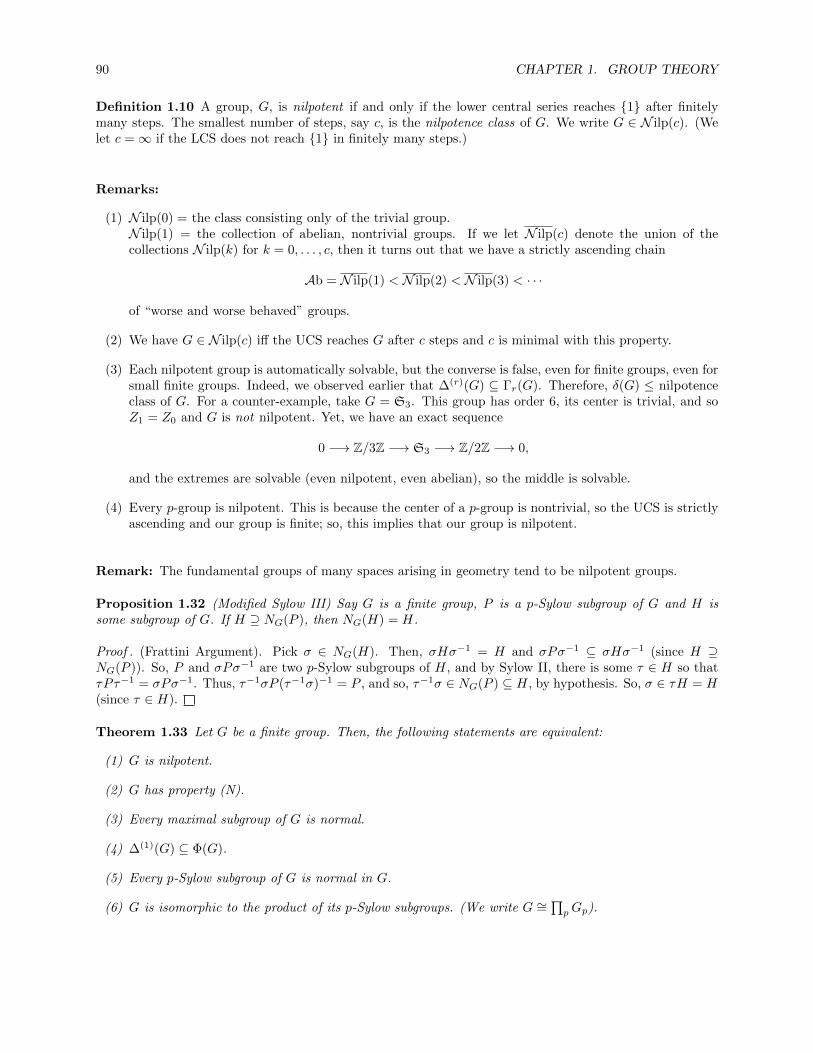
90 CHAPTER 1. GROUP THEORY
Definition 1.10 A group, G, is nilpotent if and only if the lower central series reaches 1 after finitelymany steps. The smallest number of steps, say c, is the nilpotence class of G. We write G ∈ N ilp(c). (Welet c =∞ if the LCS does not reach 1 in finitely many steps.)
Remarks:
(1) N ilp(0) = the class consisting only of the trivial group.N ilp(1) = the collection of abelian, nontrivial groups. If we let N ilp(c) denote the union of thecollections N ilp(k) for k = 0, . . . , c, then it turns out that we have a strictly ascending chain
Ab = N ilp(1) < N ilp(2) < N ilp(3) < · · ·
of “worse and worse behaved” groups.
(2) We have G ∈ N ilp(c) iff the UCS reaches G after c steps and c is minimal with this property.
(3) Each nilpotent group is automatically solvable, but the converse is false, even for finite groups, even forsmall finite groups. Indeed, we observed earlier that ∆(r)(G) ⊆ Γr(G). Therefore, δ(G) ≤ nilpotenceclass of G. For a counter-example, take G = S3. This group has order 6, its center is trivial, and soZ1 = Z0 and G is not nilpotent. Yet, we have an exact sequence
0 −→ Z/3Z −→ S3 −→ Z/2Z −→ 0,
and the extremes are solvable (even nilpotent, even abelian), so the middle is solvable.
(4) Every p-group is nilpotent. This is because the center of a p-group is nontrivial, so the UCS is strictlyascending and our group is finite; so, this implies that our group is nilpotent.
Remark: The fundamental groups of many spaces arising in geometry tend to be nilpotent groups.
Proposition 1.32 (Modified Sylow III) Say G is a finite group, P is a p-Sylow subgroup of G and H issome subgroup of G. If H ⊇ NG(P ), then NG(H) = H.
Proof . (Frattini Argument). Pick σ ∈ NG(H). Then, σHσ−1 = H and σPσ−1 ⊆ σHσ−1 (since H ⊇NG(P )). So, P and σPσ−1 are two p-Sylow subgroups of H, and by Sylow II, there is some τ ∈ H so thatτPτ−1 = σPσ−1. Thus, τ−1σP (τ−1σ)−1 = P , and so, τ−1σ ∈ NG(P ) ⊆ H, by hypothesis. So, σ ∈ τH = H(since τ ∈ H).
Theorem 1.33 Let G be a finite group. Then, the following statements are equivalent:
(1) G is nilpotent.
(2) G has property (N).
(3) Every maximal subgroup of G is normal.
(4) ∆(1)(G) ⊆ Φ(G).
(5) Every p-Sylow subgroup of G is normal in G.
(6) G is isomorphic to the product of its p-Sylow subgroups. (We write G ∼=∏pGp).

1.5. SOLVABLE AND NILPOTENT GROUPS 91
Proof . (1)⇒ (2). Let H be a proper subgroup of G, we must prove that NG(H) > H. Now, there is somec with Γc = 1. Obviously, Γc ⊆ H, so pick a smallest d for which Γd ⊆ H, so that Γd−1 6⊆ H.
Claim: Γd−1 ⊆ NG(H).
If the claim holds, then H < NG(H), i.e., G has property (N). Pick ξ ∈ Γd−1; so,
[H, ξ] ⊆ [H,Γd−1] ⊆ [G,Γd−1] = Γd.
Pick h ∈ H and look at [h−1, ξ]. The element [h−1, ξ] is in Γd, and so, in H (since Γd ⊆ H). Consequently,h−1ξhξ−1 ∈ H, from which we deduce ξhξ−1 ∈ H, and since this is true for all h ∈ H, we have ξ ∈ NG(H),as desired.
(2)⇒ (3). This has already been proved (c.f. Proposition 1.17).
(3)⇒ (4). This has already been proved (c.f. Proposition 1.23).
(4)⇒ (5). Let P be a p-Sylow subgroup of G. Look at NG(P ). If NG(P ) 6= G, then NG(P ) is containedis some maximal subgroup, M . By modified Sylow III, we get NG(M) = M . Now, ∆(1)(G) ⊆ Φ(G) ⊆M , byhypothesis, and the second homomorphism theorem implies that M corresponds to a subgroup of G/∆(1)(G)and normal subgroups correspond to normal subgroups. Yet, G/∆(1)(G) is abelian, so all its subgroups arenormal, which implies that M is normal, a contradiction.
(5)⇒ (6). This has already been proved (c.f. Proposition 1.18).
(6)⇒ (1). Since every p-group is nilpotent, the implication (6)⇒ (1) follows from the following
Proposition 1.34 Say Gj ∈ N ilp(cj), for j = 1, . . . , t. Then,
t∏
j=1
Gj ∈ N ilp( max1≤j≤t
cj).
Proof . An obvious induction reduces us to the case t = 2. In this case, we use an induction on maxc1, c2.The cases c1 ≤ 1 and c2 ≤ 1 are trivial. Now, we have (DX)
Z(G1
∏G2) ∼= Z(G1)
∏Z(G2).
But then, (G1
∏G2)/Z(G1
∏G2) ∼= (G1/Z(G1))
∏(G2/Z(G2)); on the left hand side, the purported nilpo-
tence class is down by 1 and on the righthand side, both are down by 1. We conclude by applying theinduction hypothesis.
This concludes the proof of Theorem 1.33.

92 CHAPTER 1. GROUP THEORY
1.6 Ω-Groups and the Jordan-Holder-Schreier Theorem
Let Ω be some set. If M is a group, we denote the monoid of group endomorphisms of M (under composition)by EndGr(M) and the group of (group) automorphisms of M by AutGr(M).
Definition 1.11 A group, M , is an Ω-group iff there exists a set map Ω −→ EndGr(M). If Ω is itself agroup, we demand that our map be a homomorphism (so, the image lies in AutGr(M)). If Ω is a ring, wedemand that M be an abelian group and that our map be a ring homomorphism taking 1 ∈ Ω to the identityendomorphism of M .
Examples.
(1) When Ω is a group, we get an Ω-action on M (at first, as a set) and further, we obtain:
1 ·m = m,
ξ · (η ·m) = (ξη) ·m,ξ · (mn) = (ξ ·m)(η · n).
In particular, (ξ ·m)−1 = ξ ·m−1.
(2) When Ω is a group and M is abelian, we just get an Ω-module.
(3) If Ω is a ring, then the nomenclature is Ω-module instead of Ω-group.
(4) When Ω is a field, then an Ω-module is a vector space over Ω.
(5) Being an Z-module is equivalent to being an abelian group.
An Ω-subgroup of M (resp. Ω-normal subgroup of M) is just a subgroup (resp. a normal subgroup), N ,of M stable under Ω, i.e., for all ξ ∈ Ω, for all n ∈ N , we have ξ · n ∈ N .
Blanket Assertion (DX). The three isomorphism theorems of ordinary group theory are true for Ω-groups provided everywhere “subgroup” appears we substitute “Ω-subgroup”, mutatis–mutandis for “normalsubgroups.”
Definition 1.12 A normal flag (normal series, normal chain) is a descending chain of Ω-subgroups of M :
M = M0 ⊇M1 ⊇M2 ⊇ · · · ⊇Mr = 1, (∗)
each Mj being normal in the preceding Mj−1. A normal flag is nonrepetitious if for no j do we haveMj = Mj−1. Given a second normal flag:
M = M ′0 ⊇M ′1 ⊇M ′2 ⊇ · · · ⊇M ′s = 1, (∗∗)
the flag (∗∗) refines (∗) iff for every i the Ω-group Mi occurs as some M ′j . Two normal flags (∗) and (∗∗)are isomorphic iff the collection of their successive quotients, Mi−1/Mi and M ′j−1/M
′j may be rearranged so
that, after rearrangement, they become pairwise isomorphic (in their new order). When this happens, thelengths r and s are equal.
Theorem 1.35 (Schreier refinement theorem, 1928) For an Ω-group, any two normal flags possess isomor-phic refinements. If both normal flags are nonrepetitious, so are their isomorphic refinements.
The main corollary of the Schreier refinement theorem is:
Corollary 1.36 (Jordan–Holder theorem) Any two composition series for an Ω-group are isomorphic.

1.6. Ω-GROUPS AND THE JORDAN-HOLDER-SCHREIER THEOREM 93
Proof . A composition series has no refinements except itself—apply Schreier’s theorem.
Zassenhaus proved a lemma specifically designed to give the smoothest proof of Schreier’s theorem—thisis
Lemma 1.37 (Zassenhaus’ butterfly lemma) Say G is an Ω-group and A and C are subgroups. SupposeB CA and D C C are further Ω-subgroups. Then,
(A ∩ C)B/(A ∩D)B ∼= (C ∩A)D/(C ∩B)D.
G
D
CA
B
B ! C A ! D
A ! C
Figure 1.1: The butterfly lemma
Proof . Let T = A ∩ C = C ∩A, M = B ∩ C and N = A ∩D. The conclusion of the lemma is
TB/NB ∼= TD/MD.
First of all, there is right-left symmetry in the statement of the lemma and its conclusion (A↔ C, B ↔ D;under these substitutions, T ↔ T and M ↔ N). We must prove that NB C TB. Pick t ∈ G and look attNBt−1 = tNt−1tBt−1. If t ∈ A, then tBt−1 = B, since B CA. Thus, if t ∈ A then tNBt−1 = tNt−1B. Ift ∈ T ⊆ C, then as N = D ∩ C ∩A = D ∩ T and D C C, we get
tNt−1 = tDt−1 ∩ tT t−1 = tDt−1 ∩ T = D ∩ T = N.
Thus, if t ∈ T then tNBt−1 = NB.
Say ξ = tb ∈ TB. Since B CA and N ⊆ A, we have BN = NB. Then, we find
ξNBξ−1 = tbNBb−1t−1
= tbNBt−1
= tbBNt−1
= tBNt−1
= tNBt−1
= NB.
Therefore, NB C TB. By symmetry, we get MD C TD. Look at TB/NB = TNB/BN (since N ⊆ T ). Bythe third isomorphism theorem, we have
TB/NB ∼= T/T ∩NB.

94 CHAPTER 1. GROUP THEORY
By symmetry,TD/ND ∼= T/T ∩MD.
If we prove that T ∩ NB = T ∩ NM (and so, T ∩ MD = T ∩ NM , by symmetry), we will be done.Pick ξ ∈ T ∩ NB. We can write ξ = nb ∈ NB, so b = n−1ξ ∈ NT = T (since N ⊆ T ). Thus,b ∈ B ∩ T = B ∩ C ∩ A ⊆ M , and so, b ∈ M . Consequently, ξ = nb ∈ NM and since we also have ξ ∈ T ,then ξ ∈ T ∩ NM . This proves that T ∩ NB ⊆ T ∩ NM . The reverse inclusion is trivial, since M ⊆ B.Therefore, T ∩NB = T ∩NM , as claimed.
Proof of Theorem 1.35. Let
M = M0 ⊇M1 ⊇M2 ⊇ · · ·Mi−1 ⊇Mi ⊇ · · · ⊇Mr = 1, (∗)
and
M = M ′0 ⊇M ′1 ⊇M ′2 ⊇ · · ·M ′j−1 ⊇M ′j ⊇ · · · ⊇M ′s = 1, (∗∗)
be two normal nonrepetitious chains. Consider the groups
M(j)i−1 = (Mi−1 ∩M ′j)Mi.
As j varies, these groups start at Mi−1 (= M(0)i−1) and end at Mi (= M
(s)i−1) and we get a refinement of (∗) if
we do this between any pair in (∗). Also consider the groups
M′(i)j−1 = (M ′j−1 ∩Mi)M
′j ,
and let i vary. These groups interpolate between M ′j−1 and M ′j , just as above. Look at the successivequotients
M(j−1)i−1 /M
(j)i−1; M
′(i−1)j−1 /M
′(i)j−1. (†)
If we let A = Mi−1, B = Mi (C A), C = M ′j−1 and D = M ′j (C C), we can write the first quotient group of(†) as
M(j−1)i−1 /M
(j)i−1 = (Mi−1 ∩M ′j−1)Mi/(Mi−1 ∩M ′j)Mi = (A ∩ C)B/(A ∩D)B,
the left hand side of Zassenhaus’ lemma. By symmetry, the second quotient group of (†) is the righthandside of Zassenhaus’ lemma and we are done.

1.7. CATEGORIES, FUNCTORS AND FREE GROUPS 95
1.7 Categories, Functors and Free Groups
Definition 1.13 A category , C, is a pair: 〈Ob(C),F l(C)〉, in which Ob(C) and F l(C) are classes, called theobjects of C and the morphisms (or arrows) of C, respectively. We require the following conditions:
(1) For all A,B ∈ Ob(C), there is a unique set, HomC(A,B), called the collection of morphisms from Ato B, and any two such are either disjoint or equal. Further
F l(C) =⋃
A,B
HomC(A,B).
For the morphisms, we also require:
(2) For every u ∈ HomC(A,B) and v ∈ HomC(B,C), there exists a unique morphismw = v u ∈ HomC(A,C), called the composition of v and u.
(3) For every A ∈ Ob(C), there is some arrow, 1A ∈ HomC(A,A), so that for every B ∈ Ob(C) andu ∈ HomC(A,B), we have
A1A−→ A
u−→ B = Au−→ B
Au−→ B
1B−→ B = Au−→ B.
Note: This shows that 1A is unique for each A (DX).
(4) We have the associativity lawu (v w) = (u v) w,
whenever the compositions all make sense.
Examples of Categories:
(1) Sets, the category of sets; Ob(Sets) = all sets, F l(Sets) = all maps of sets.
(2) Gr, the category of groups; Ob(Gr) = all groups, F l(Gr) = all homomorphisms of groups. A specialcase is Ab, the category of abelian groups.
(3) Ω-Gr, the category of Ω-groups. Special cases are: The category of G-modules,Mod(G); the categoryof R-modules, Mod(R) (where R is a ring); and the category of vector spaces, Vect(k) (where k is afield). Also, Ab =Mod(Z).
(4) TOP, the category of topological spaces; Ob(TOP) = all topological spaces,F l(TOP) = all continuous maps.
(5) Ck-MAN, the category of Ck-manifolds; Ob(Ck-MAN) = all (real) Ck-manifolds (0 ≤ k ≤ ∞ or ω),F l(Ck-MAN) = all Ck-maps of Ck-manifolds.
(6) HOL, the category of complex analytic manifolds; Ob(HOL) = all complex analytic manifolds,F l(HOL) = all complex analytic maps of holomorphic manifolds.
(7) RNG, the category of all rings; Ob(RNG) = all rings (with unity), F l(RNG) = all homomorphisms ofrings. A special case is CR, the category of commutative rings.
A subcategory , D, of C is a category, 〈Ob(D),F l(D)〉, so that
(a) Ob(D) ⊆ Ob(C).

96 CHAPTER 1. GROUP THEORY
(b) F l(D) ⊆ F l(C), in such a way that for all A,B ∈ Ob(D), we haveHomD(A,B) ⊆ HomC(A,B).
We say that D is a full subcategory of C iff for all A,B ∈ Ob(D), we haveHomD(A,B) = HomC(A,B).
Examples of Subcategories:
(1) The category, Ab, is a full subcategory of Gr; the category, CR, is a full subcategory of RNG.
(2) Recall that u ∈ HomC(A,B) is an isomorphism (in C) iff there is some v ∈ HomC(B,A) so that
Au−→ B
v−→ A = A1A−→ A
Bv−→ A
u−→ B = B1B−→ B.
Take D so that Ob(D) = Ob(C), and morphisms, setHomD(A,B) = u ∈ HomC(A,B) | u is an isomorphism and F l(D) =
⋃A,B HomD(A,B). (Note that
HomD(A,B) may be empty.) The category, D, is generally a nonfull subcategory of C, for examplewhen C = Sets.
Say C is a category, we can make a new category, CD, the dual or opposite category , as follows: Ob(CD) =Ob(C) and reverse the arrows, i.e., for all A,B ∈ Ob(C),
HomCD (A,B) = HomC(B,A).
Definition 1.14 Let C and C′ be categories. A functor (respectively, a cofunctor), F , from C to C′ is a rulewhich associates to each object A ∈ Ob(C) an object F (A) ∈ Ob(C′) and to each arrow u ∈ HomC(A,B) anarrow F (u) ∈ HomC′(F (A), F (B)) (resp. F (u) ∈ HomC′(F (B), F (A))) so that,
F (1A) = 1F (A)
F (u v) = F (u) F (v)
(resp. F (u v) = F (v) F (u), for cofunctors.)
Remark: Obviously, Definition 1.14 can be made more formal by defining a functor, F , from C to C′ as apair, 〈F ob, F fl〉, where F ob : Ob(C) → Ob(C′) and F fl : F l(C) → F l(C′), so that, for every u ∈ HomC(A,B),we have F fl(u) ∈ HomC′(F
ob(A), F ob(B)), and the conditions of Definition 1.14 hold (and similarly forcofunctors).
We use the notation A F (A) (or u F (u)) to indicate that F : C → C′ is a functor from C to C′, andnot just an ordinary function.
Examples of Functors
(1) For the categories in Examples (2)–(7), consider the rule:A ∈ Ob(C) |A| = the underlying set of A, andu ∈ F l(C) |u| = the morphism, u, as a map of sets.The functor, | |, is a functor from C to Sets, called the forgetful functor or stripping functor .
(2) A cofunctor, F : C → C′, is just a functor, F : CD → C′ (equivalently, F : C → C′D).
(3) We have the functor, Ga : RNG → Ab, given by taking Ga(R) = R as an additive group, for everyring, R. The functor, Ga, is called the additive group functor .

1.7. CATEGORIES, FUNCTORS AND FREE GROUPS 97
(4) For every integer, n ≥ 0, we have the functor, GLn : CR→ Gr, where GLn(A) is the group of invertiblen×n matrices with entries in A. When n = 1, the group GL1 is denoted Gm. This is the multiplicativegroup functor , it takes CR to Ab. The functor Gm can be promoted to a functor, RNG −→ Gr, takingthe ring, A, to its group, A∗, of units.
(5) Let (TOP, ∗) be the category of topological spaces together with a base point. We have the subcategory(C-TOP, ∗) consisting of connected and locally connected topological spaces with a base point. Themorphisms of (C-TOP, ∗) preserve base points. We have the functors (fundamental group)
π1 : (C-TOP, ∗)→ Gr,
and for n > 1 (nth homotopy group),
πn : (C-TOP, ∗)→ Ab.
(6) For every integer, n ≥ 0, we have a functor (integral homology), TOP −→ Ab, given by X Hn(X,Z)and a cofunctor (integral cohomology), TOP −→ Ab, given by X Hn(X,Z).
(7) math.upenn.edu/ Given a group, G, for any integer, n ≥ 0, we have a functor,Mod(G) −→ Ab, givenby A Hn(G,A).
Definition 1.15 Say F and F ′ are two functors C −→ C′. A morphism, θ, from F to F ′ is a collectionθA | A ∈ Ob(C), where:
(1) θA : F (A)→ F ′(A) in C′, so that (consistency)
(2) For every v : A→ B in C, the diagram
F (A)
F (v)
θA // F ′(A)
F ′(v)
F (B)
θB // F ′(B)
commutes, for all A,B ∈ Ob(C).A morphism of functors is also called a natural transformation of functors.
Examples of Morphisms of Functors:
(1) In the category (C-TOP, ∗), we have the functors π1 and H1(−,Z). The Hurewicz map
π1(X)uX−→ H1(X,Z)
defines a morphism of functors.
(2) If G is a group and K is a subgroup of G, we have the obvious restriction functorres : Mod(G)→Mod(K), and it induces a morphism of functors res : Hn(G,−)→ Hn(K,−).
(3) The determinant, det : GLn → Gm, is a morphism of functors (from CR to Ab).
(4) Check (DX) that with the above notion of morphisms, the functors from C to C′ form a categorythemselves. This category is denoted Fun(C, C′).
Proposition 1.38 Given a category, C, each object, A, of C gives rise to both a functor, hA, and a cofunctor,hDA , from C to Sets.

98 CHAPTER 1. GROUP THEORY
Proof . For any given A ∈ Ob(C), let
hA(B) = HomC(A,B)
hDA (B) = HomC(B,A).
Moreover, for every v ∈ HomC(B,C), define hA(v) : HomC(A,B)→ HomC(A,C) by composition, so that forevery u ∈ HomC(A,B),
hA(v)(u) = v u,and, for every v ∈ HomC(B,C), define hDA (v) : HomC(C,A) → HomC(B,A), again by composition, so thatfor every u ∈ HomC(C,A),
hDA (v)(u) = u v.The reader should check that hA and hDA are indeed functors (DX).
The following proposition is half of the Yoneda embedding lemma:
Proposition 1.39 Let A and A be two objects of C and suppose that the corresponding functors hA andhA are isomorphic, say by θ : hA → hA. Then, A and A are isomorphic via a canonically determinedisomorphism (dependent on θ).
Proof . For every B ∈ Ob(C), we have an isomorphism
θB : HomC(A,B) −→HomC(A, B),
and this is functorial. Let B = A, then θA : HomC(A,A)−→HomC(A, A), and we set ψ = θA(1A), a morphism
in HomC(A, A). Now, if we let B = A, we get θA : HomC(A, A) −→HomC(A, A), and we set ϕ = θ−1
A(1A), a
morphism in HomC(A, A). Pick any z in HomC(A,B). We would like to understand what θB(z) is. We havethe commutative diagram
z ∈ HomC(A,B)θB // HomC(A, B)
1A ∈ HomC(A,A)
z−
OO
θA
// HomC(A, A).
z−
OO
Following the above commutative diagram clockwise, we get θB(z), and following it counterclockwise, we getz ψ. We conclude that
θB(z) = z ψ.Similarly, for any z ∈ HomC(A, B), by considering the commutative diagram involving θ−1
Aand θ−1
B , we get
θ−1B (z) = z ϕ.
But then, we have1A = θA(ϕ) = ϕ ψ and 1A = θ−1
A (ψ) = ψ ϕ,which shows that ϕ and ψ are inverse isomorphisms. Furthermore, ϕ (resp. ψ) determine θ, just as θdetermines ϕ and ψ.
Example. Recall that Vect(k) is the category of vector spaces over a field, k. There exists a cofunctor,D : Vect(k) −→ Vect(k), given by: V V D = HomVect(k)(V, k) = the dual space of V ; and for any linearmap, θ : V → W , the map θD : WD → V D is the adjoint of θ. By applying D again, we get a functor,DD : Vect(k) −→ Vect(k). However, it is well-known that there exists a morphism of functors,
η : id→ DD, where id(V ) = VηV−→ DD(V ) = V DD, and this is functorial.
Two categories, C and C′, are equivalent (resp. isomorphic) iff there exist functors F : C → C′ andF ′ : C′ → C so that F ′ F ∼= 1C and F F ′ ∼= 1C′ (resp. F ′ F = 1C and F F ′ = 1C′). Here 1C denotes theidentity functor from C to itself.

1.7. CATEGORIES, FUNCTORS AND FREE GROUPS 99
Proposition 1.40 (Yoneda’s Embedding Lemma) The functor A hDA establishes an equivalence of thecategory, C, with a full subcategory of FunD(C,Sets) (where FunD(C, C′) denotes the category of cofunctorsfrom C to C′).
Proof . We already know from Proposition 1.39 that if we have an isomorphism θ : hDA → hDA
, then θ de-
termines uniquely two mutually inverse isomorphisms ψ : A → A and ϕ : A → A. So, two objects A andA in Ob(C) give isomorphic cofunctors iff they themselves are isomorphic. Given any v ∈ HomF (hDA , h
DA
),
where F = FunD(C,Sets), we know (again) that there exists a morphism ψ : A → A, so that v is given bycomposing with ψ, i.e., given a consistent family of morphisms, vB : hDA (B)→ hD
A(B), that is,
vB : HomC(B,A) → HomC(B, A), we have vB(z) = ψ z, and our ψ is given by ψ = vA(1A) (all this from
the proof of Proposition 1.39). Hence, from v, we get a morphism ψ : A→ A, thus
HomC(A, A) ∼= HomF (hDA , hDA
).
So, we indeed have an equivalence with a full subcategory of F , namely the image consists of those cofunctorsof the form hDA (easy details are left to the reader (DX)).
Remark: What does Yoneda’s lemma say? It says that any object A ∈ Ob(C) is determined by its corre-sponding cofunctor hDA . The cofunctor, hDA , is a “collection of interconnected sets”, HomC(B,A) being theset associated with B.
Definition 1.16 Given a functor, F , from C to Sets (resp. a cofunctor, G, from CD to Sets), it is repre-sentable iff there exists a pair, (A, ξ), where A ∈ Ob(C) and ξ ∈ F (A), so that F is isomorphic to hA via the
morphism of functors, ξ : hA → F , given by the consistent family of morphisms ξB : HomC(A,B) → F (B)defined via
ξB(u) = F (u)(ξ),
(resp. G is isomorphic to hDA via the morphism of functors, ξ : hDA → G, given by ξB : HomC(B,A)→ G(B).
Here, ξB is defined via ξB(u) = G(u)(ξ)).
The notion of representable functor is a key concept of modern mathematics. The underlying idea is to“lift” as much as possible of the knowledge we have about the category of sets to other categories. Morespecifically, we are interested in those functors from a category C to Sets that are of the form hA for someobject A ∈ Ob(C).
Remark: If (A, ξ) and (A′, ξ′) represent the same functor, then there exists one and only one isomorphism
A −→ A′ so that ξ ∈ F (A) maps to ξ′ ∈ F (A′). This is because we have the isomorphisms ξ : hA−→ F and
ξ′ : hA′−→ F ; and so, we have an isomorphism ξ′−1 ξ : hA−→ hA′ . By Yoneda’s lemma, A−→ A′ via the
isomorphism determined by ξ and ξ′ and this maps ξ to ξ′. Uniqueness follows as everything is determinedby ξ and ξ′.
Examples of Representable Functors:
(1) Let C = Sets; consider the functor F : SetsD → Sets given by: F (S) = the collection of all subsets ofS, and if θ : S → T is a map of sets, the morphism F (θ) : F (T ) → F (S) is the map that sends everysubset, V , of T to its inverse image, θ−1(V ), a subset of S. Is this a representable functor?
We need a set, Q, and an element, ξ ∈ F (Q), i.e., some subset of Q, so that
hDQ(B) = HomSets(B,Q) −→ F (B), via ξB(u) = F (u)(ξ).

100 CHAPTER 1. GROUP THEORY
Now, we know that F (u) : F (Q)→ F (B) is the map that sends a subset, S, of Q to its inverse image,u−1(S), a subset of B. So, F (u)(ξ) is the inverse image of our chosen ξ.
Take Q = 0, 1 and ξ = 1 ⊆ Q. Then, subsets of B are exactly of the form, u−1(1), for the variousu ∈ HomSets(B,Q), which are thus characteristic functions.
(2) Let C = RNG, and let F : RNG→ Sets be the stripping functor. Is it representable?
We need a ring, P , and an element, ξ ∈ P , so that for all rings, B,
HomRNG(P,B) −→ |B|,
viau ∈ HomRNG(P,B) 7→ u(ξ) ∈ |B|.
Take P = Z[T ], the polynomial ring in one variable with integral coefficients, and ξ = T . Then, anyring homomorphism u ∈ HomRNG(Z[T ], B) is uniquely determined by u(T ) = b ∈ |B|, and any b canbe used.
Definition 1.17 Let F : C → C′ and G : C′ → C be two functors. The functor F is the left (resp. right)adjoint of G iff for every A ∈ Ob(C) and B ∈ Ob(C′), we have functorial isomorphisms (in both A and B)
HomC′(F (A), B) −→ HomC(A,G(B)).
(resp. HomC′(B,F (A)) −→ HomC(G(B), A)).
Observe that F is left-adjoint to G iff G is right-adjoint to F . Many so-called “universal constructions”arise from the existence of adjoint functors; this is a key concept in modern mathematics.
Remark: The concept of adjointness is related to the notion of representability of a functor, as shown by thefollowing proposition whose simple proof is left to the reader:
Proposition 1.41 A functor, G : C′ → C, has a left-adjoint if and only if, for every A ∈ C, the functor B HomC(A,G(B)) from C′ to Sets is representable. If (F (A), ξ) represents this functor (so that ξB : HomC′(F (A), B) ∼=HomC(A,G(B)) is an isomorphism for every B ∈ C′), then F is the object part of a left-adjoint of G for which the
isomorphism ξB is functorial in B and yields the adjointness.
A functor may have a right adjoint, but no left adjoint, and conversely (or no adjoint at all). For example,the functor, G G/[G,G] = Gab, from Gr to Ab, is the left adjoint of the inclusion functor from Ab to Gr.The inclusion views an abelian group just as a group. So, G Gab has a right adjoint. However, we nowprove that it has no left adjoint.
Suppose such a left adjoint, F , exists.
Claim 1: For any abelian group, H, the group F (H) can never be simple unless F (H) = 1, in whichcase, H = 1.
The adjointness property states that for every group, G, we have a functorial isomorphism
HomGr(F (H), G) ∼= HomAb(H,Gab). (∗)
If we take G = F (H) in (∗), we have
HomGr(F (H), F (H)) ∼= HomAb(H,F (H)ab).
If F (H) 6= 1 and F (H) is non-abelian simple, then, on the left hand side there are at least two maps(id and the constant map that sends all elements to 1), even though on the righthand side there is a single

1.7. CATEGORIES, FUNCTORS AND FREE GROUPS 101
map, since F (H) is non-abelian simple, a contradiction. If F (H) is Z/pZ for some prime p, take G in (∗)to be A3p. Again, there are at least two maps in HomGr(F (H), A3p), namely: the constant map and anembedding. But A3p is simple; so, the righthand side has only one element, again a contradiction. Now, ifF (H) = 1, take G = H in (∗). In this case, the left hand side has a single map but the righthand side hasat least two maps if H 6= 1.
Claim 2: F (H) has no maximal normal subgroups. If M C F (H) and M is maximal, then F (H)/Mis simple. Let G = F (H)/M in (∗). If F (H)/M is non-abelian, there are at least two maps on the lefthand side, but only one on the righthand side, a contradiction. If F (H)/M is abelian, say Z/pZ, againtake G = A3p in (∗). There are two maps (at least) on the left hand side (stemming from the two mapsF (H) −→ F (H)/M) and only one on the righthand side. So, if F (H) exists, it is not finitely generated.
Take H = G = Z/2Z. Then, we have
HomGr(F (Z/2Z),Z/2Z) ∼= HomAb(Z/2Z,Z/2Z).
Clearly, the righthand side has exactly two maps, and thus, so does the left hand side. But one of thesemaps is the constant map sending all elements to 1, so the other map must be surjective. If so, its kernel,K, is a subgroup of index 2, hence normal, and so, it must be maximal normal, a contradiction.
Therefore, the functor G G/[G,G] = Gab, from Gr to Ab, has no left adjoint.
One often encounters situations (for example in topology, differential geometry and algebraic geometry)where the objects of interest are arrows “over” a given object (or the dual notion of arrows “co-over” a givenobject), for example, vector bundles, fibre bundles, algebras over a ring, etc. Such situations are capturedby the abstract notion of “comma categories.”
Definition 1.18 Let C be a category and fix some object, A, in Ob(C). We let CA, the category over A(or comma category), be the category whose objects are pairs (B, πB), where B is some object in Ob(C)and πB is a morphism in HomC(B,A), and whose morphisms from (B, πB) to (C, πC) are the morphismsu ∈ HomC(B,C) making the following diagram commute:
Bu //
πB @@@
@@@@
@ C
πC~~
A
Dually, we let CA, the category co- over A (also called comma category), be the category whose objects arepairs (B, iB), where B is some object in Ob(C) and iB is a morphism in HomC(A,B), and whose morphismsfrom (B, iB) to (C, iC) are the morphisms u ∈ HomC(B,C) making the following diagram commute:
Bu // C
A
iB
__@@@@@@@@ iC
>>
The notion of representable functor allows us to define products and coproducts in arbitrary categories.
Let C be any category. Say Aαα∈Λ is a set of objects in Ob(C).(1) We get a cofunctor, F , from CD to Sets via
B ∏
α
HomC(B,Aα) = F (B),
where the above product is just the cartesian product of sets, and

102 CHAPTER 1. GROUP THEORY
(2) We get a functor, G, from C to Sets via
B ∏
α
HomC(Aα, B) = G(B).
Are these (or either) representable?
First, consider (1). We need an object, P ∈ Ob(C) and some ξ ∈ F (P ), i.e. ξ ∈∏α HomC(P,Aα), whichmeans that ξ = prαα, where the prα are morphisms prα : P → Aα.
Definition 1.19 When (P, prα) exists, i.e. for every B ∈ Ob(C), there is a functorial isomorphism
HomC(B,P ) −→∏
α
HomC(B,Aα),
via u 7→ (prα u)α, the pair (P, prα) is the product of the Aα’s in C. This product is denoted∏αAα (one
usually drops the prα’s). We have the (functorial) isomorphism
HomC(B,∏
α
Aα) −→∏
α
HomC(B,Aα). (∗)
Remark: Definition 1.19 implies that for every family of morphisms,fα : B → Aα ∈
∏α HomC(B,Aα), there is a unique morphism, u : B →
∏αAα, so that
fα = prα u, for all α.
This is called the universal mapping property of products. In general, universal mapping properties are another name
for representing a functor. The latter is a more general and supple notion and we will mainly stick to it.
Now, consider (2). We need an object, Q ∈ Ob(C), and some ξ ∈ G(Q), i.e. ξ ∈∏α HomC(Aα, Q), whichmeans that ξ = iαα, where the iα are morphisms iα : Aα → Q.
Definition 1.20 When (Q, iα) exists, i.e. for every B ∈ Ob(C), there is a functorial isomorphism
HomC(Q,B) −→∏
α
HomC(Aα, B),
via u 7→ (u iα)α, the pair (Q, iα) is the coproduct of the Aα’s in C. This coproduct is denoted∐αAα
(one usually drops the iα’s). We have the (functorial) isomorphism
HomC(∐
α
Aα, B) −→∏
α
HomC(Aα, B). (∗∗)
Of course, as above, there is a universal mapping property here, also.
Definition 1.21 The product in CA is called the fibred product over A in C. The coproduct in CA is calledthe fibred coproduct over A in C.
Remark: Given any family, (Aα, πα)α, of objects in CA (with πα : Aα → A), the fibred product of the Aα’s overA in C is a pair, (
∏A
Aα, ξ), where∏A
Aα is some object in C (together with a morphism, π :∏A
Aα → A), and ξ
consists of a family of morphisms, prα :∏A
Aα → Aα, with
πα prα = πβ prβ (= π), for all α, β;

1.7. CATEGORIES, FUNCTORS AND FREE GROUPS 103
moreover, for any object, B ∈ C, and any family of morphisms, fα : B → Aαα, with
πα fα = πβ fβ , for all α, β,
there is a unique morphism, u : B →∏A
Aα, so that fα = prα u, for all α.
We leave it to the reader to unwind the definition of fibred coproducts over A in C.
Examples of Products, Coproducts, Fibred Products and Fibred Coproducts:
(1) C = Sets. Given a family of sets, Aαα∈Λ, does∏αAα or
∐αAα exist? If so, what are they?
For∏αAα, we seek a set, P , and an element, ξ, in F (P ), where F is the cofunctor
T F (T ) =∏
α
HomSets(T,Aα).
This means that ξ ∈ F (P ) is just a tuple of maps, prα : P → Aα. Take P to be the ordinary cartesianproduct of the Aα’s and prα : P → Aα, the αth projection. Check that this works (DX).
For∐αAα, we seek a set, Q, and an element, ξ, in G(Q), where G is our functor
T G(T ) =∏
α
HomSets(Aα, T ).
So, we need a family of maps iα : Aα → Q. Now, if Q is to work, then for every T , we need an isomorphism
θT : HomSets(Q,T ) −→∏
α
HomSets(Aα, T )
given by θT (ϕ) = (ϕ iα)α. Take Q =⋃· αAα (the disjoint union of the Aα’s). The rest of the construction
is easy (DX).
(2) C = Ab, more generally, C =Mod(R) (R a ring) or C =Mod(G) (G a group).
We begin with products. Given a family, Aαα∈Λ, with each Aα inMod(R), we seek P ∈Mod(R) andmaps prα : P → Aα in Mod(R), so that for every T ∈Mod(R), there is an isomorphism
θT : HomR(T, P ) −→∏
α
HomR(T,Aα),
where θT (ϕ) = prα ϕα (the notation HomR(A,B) is usually used, instead of the more accurate but morecumbersome notation HomMod(R)(A,B)). We see that P must be
∏αAα, the product in the category of
sets, if this can be made an R-module. Now,∏αAα is an R-module via coordinatewise addition, with the
R-action given by r(ξα) = (rξα). So,∏αAα is the product of the Aα’s in Mod(R).
Next, we consider coproducts. We seek Q ∈ Mod(R) and maps iα : Aα → Q in Mod(R), so that forevery T ∈Mod(R), there is an isomorphism
θT : HomR(Q,T ) −→∏
α
HomR(Aα, T ),
where θT (ϕ) = ϕ iαα. The disjoint union⋃· αAα may be a first approximation to Q, but it is not good
enough. Instead, we let
Q =ξ ∈
∏
α
Aα | prα(ξ) = 0 for all but finitely many α.

104 CHAPTER 1. GROUP THEORY
This is an R-submodule of∏αAα. The isomorphism
θT : HomR(Q,T ) −→∏
α
HomR(Aα, T )
can now be established. First, let iα(u) = (δuβ)β , where δuα = u and δuβ = 0 for all β 6= α. Given a family,(ϕα)α, of maps ϕα : Aα → T , for any ξ = (ξα)α ∈ Q, set ϕ(ξ) =
∑α ϕα(ξα) ∈ T . If ϕ ∈ HomR(Q,T ) is
given, define ϕα = ϕ iα. This shows that if we set∐αAα to be our R-module Q and the iα to be our
maps, iα : Aα → Q, as above, we have proved the proposition:
Proposition 1.42 The categories: Sets, Ab, Mod(R), Mod(G) all possess arbitrary products and coprod-ucts.
How about fibred products and coproducts?
(3) Let us go back to C = Sets, and first consider fibred products over A. A first approximation to theproduct, P , in SetsA, is
∏αAα. However, this is not good enough because there is no “structure map”,
π : P → A, so that
Pprα //
π@
@@@@
@@@ Aα
πα
A
commutes for all α. We let
PA =ξ ∈
∏
α
Aα | πα(ξα) = πβ(ξβ), for all α, β.
This is a set (possibly empty), and it lies over A; indeed, we can define π : PA → A by π(ξ) = πα(ξα), for anychosen α, since this is well-defined by definition of PA. We write
∏A
Aα for PA and, for every α, we define
the map, prα :∏A
Aβ → Aα, as the restriction of prα :∏Aβ → Aα to
∏A
Aα. The reader should check that
this yields products in SetsA.
Coproducts are a bit harder. It is natural to try⋃· αAα as a first approximation, but this is not good
enough: this does not tell us what i : A → Q is. The difficulty is that⋃· αAα is too big, and we need to
identify some of its elements. To do so, we define an equivalence relation on⋃· αAα, in two steps. First, we
define immediate equivalence. Given ξ ∈ Aα and η ∈ Aβ , we say that ξ and η are immediately equivalent ,denoted ξ ≈ η, iff there is some a ∈ A, so that ξ = iα(a) and η = iβ(a). The relation ≈ is clearly reflexiveand symmetric but it is not necessarily transitive. So, we define ∼ to be the equivalence relation generatedby ≈. This means that ξ ∼ η iff there exist x0, . . . , xt ∈
⋃· αAα, so that
ξ = x0, x0 ≈ x1, x1 ≈ x2, . . . , xt−1 ≈ xt, xt = η.
(For example, if ξ ≈ x and x ≈ η, then ξ = iα(a), x = iβ(a), x = iβ(b) and η = iγ(b). Note thatiβ(a) = iβ(b).) We let
∐A
Aα = (⋃· αAα) / ∼, and i : A → ∐
A
Aα is given by i(a) = class of iα(a), for any
fixed α (this is well-defined, by definition of ∼). The verification that∐A
Aα works is left as an exercise
(DX). Therefore, the category of sets has arbitrary fibred coproducts as well .
(4) C = Ab, Mod(R), Mod(G).
For fibred products, we use∏A
Aα, as constructed for Sets, but made into an R-module (resp. G-module),
in the usual way.

1.7. CATEGORIES, FUNCTORS AND FREE GROUPS 105
For fibred coproducts, begin with∐αAα (in C), and define N to be the submodule generated by the
elements iα(a)− iβ(a) with a ∈ A and α, β arbitrary. Take
∐
A
Aα =
(∐
α
Aα
)/N.
Again, the reader should check that∐A
Aα works (DX). Therefore, Ab,Mod(R),Mod(G), all have arbitrary
fibred products and coproducts.
We now consider products and coproducts in the category of groups, Gr. There is no difficulty forproducts: Use
∏αAα, the usual cartesian product of the Aα’s, as sets, and make
∏αAα into a group under
coordinatewise multiplication. The same idea works for fibred products. However, coproducts require a newidea.
Given the family of groups, Aαα∈Λ, write A0α = Aα − 1. Let
S =⋃·α
A0α,
and consider, Sn, the n-fold cartesian product of S. We can view Sn as the set of words of length n overthe alphabet S; each word is an n-tuple, (σα1
, . . . , σαn), with σβ ∈ Aβ . We call such a word admissible iffAαj 6= Aαj+1
, for j = 1, 2, . . . , n− 1. Let Sn∗ denote the set of admissible words of length n, and let
Q =
(⋃
n≥1
Sn∗)∪ ∅.
(The special word, ∅, is the “empty word”.) Multiplication in Q is defined as follows:Given (σ) = (σα1
, . . . , σαr ) and (τ) = (τβ1, . . . , τβs) in Q, set
(σ)(τ) = (σα1, . . . , σαr , τβ1
, . . . , τβs),
the result of concatenating the r-tuple, (σ), with the s-tuple, (τ). In case one of (σ) or (τ) is ∅, theconcatenation is just the non-empty word and ∅∅ is ∅. The word (σ)(τ) is admissible of length r+ s, exceptif αr = β1, in which case we need to perform a reduction process to obtain an admissible word:
(1) Form σαrτβ1in Aαr = Aβ1
. There are two cases:
(a) σαrτβ16= 1αr (= 1β1
); then
(σα1, . . . , σαr−1
, σrτβ1, τβ2
, . . . , τβs)
is an admissible word of length r + s− 1, and the reduction process ends with this word as output.
(b) σαrτβ1= 1αr (= 1β1
); then, omit σαr and τβ1, form
(σα1, . . . , σαr−1
, τβ2, . . . , τβs),
a word of length r + s− 2, and if necessary, go back to (1) above.
Since both step (a) and (b) decrease the length of the current word, the reduction process must end withsome admissible word of length l ≤ r + s, or the empty word.
The set Q with the above multiplication is indeed a group with identity element, ∅ (DX). (The mapiα : Aα → Q sends σ ∈ Aα to the length-one word (σ) if σ 6= 1 or to ∅ if σ = 1.) In summary, we get

106 CHAPTER 1. GROUP THEORY
Theorem 1.43 The category of groups, Gr, possesses arbitrary coproducts (old fashioned name: “free prod-uct of the Aα.”)
Definition 1.22 Given any set, S, define the the free group on S to be the group Fr(S) =∐S
Z.
We have just shown that coproducts exist in the category Gr. What about coproducts in the categoryGrA, where A is any group?
Given a family (Gα, iα)α∈Λ in GrA, form G =∐αGα, in the category Gr. In G, consider the collection
of elementsiα(a)i−1
β (a) | a ∈ A, iα : A→ Gα, α and β ∈ Λ;let N be the normal subgroup of G generated by the above elements. Then, G/N ∈ Ob(GrA), becausethe map i : A → G/N given by i(a) = image of iα(a) in G/N (for any fixed α) is well-defined (since imageof iα(a) = image of iβ(a) in G/N). Check that, (DX), (G/N, i) is the fibred coproduct of the Gα’s. (Oldterminology: amalgamated product of the Gα over A.)
Examples of fibred coproducts: (1) Let U and V be two sets. Form the intersection U ∩ V ; we haveinclusion maps iU : U ∩ V → U and iV : U ∩ V → V . We know that U q V = U ∪· V , the disjoint union of Uand V , and then, the set-theoretic union of U and V is given by
U ∪ V = U∐
U∩VV.
(2) Consider the category (TOP, ∗) of (“nice”, i.e., connected, locally connected) topological spaces witha base point. Given two spaces (U, ∗) and (V, ∗) in (TOP, ∗), consider (U ∩ V, ∗). Then, again,
(U ∪ V, ∗) = (U, ∗)∐
(U∩V,∗)
(V, ∗), in (TOP, ∗).
Van Kampen’s theorem says that
π1(U ∪ V, ∗) = π1(U, ∗)∐
π1(U∩V,∗)
π1(V, ∗),
which may also be written as
π1
((U, ∗)
∐
(U∩V,∗)
(V, ∗))
= π1(U, ∗)∐
π1(U∩V,∗)
π1(V, ∗).
In other words, van Kampen’s theorem says that π1 commutes with fibred coproducts.
Go back to the free group, Fr(S). We have
HomGr(Fr(S), G) = HomGr(∐
S
Z, G)
∼=∏
S
HomGr(Z, G)
∼=∏
S
|G| = HomSets(S, |G|).
Corollary 1.44 The functor, S Fr(S), from Sets to Gr is the left adjoint to the stripping functor,G |G|, from Gr to Sets.

1.7. CATEGORIES, FUNCTORS AND FREE GROUPS 107
Corollary 1.45 If S −→ T is surjective, then Fr(S) −→ Fr(T ) is a surjection of groups. Also,Fr(S) ∼= Fr(T ) iff #(S) = #(T ) (i.e., S and T have the same cardinality).
Proof . If u : S → T is a surjection in Sets, then there is a map v : T → S so that u v = 1T . Since Fr is afunctor, we get homomorphisms Fr(u) : Fr(S)→ Fr(T ) and Fr(v) : Fr(T )→ Fr(S); also, Fr(u)Fr(v) = 1Fr(T ),which shows that Fr(u) is surjective.
If #(S) = #(T ), it is obvious that Fr(S) ∼= Fr(T ). Conversely, assume that Fr(S) ∼= Fr(T ). We knowthat
HomGr(Fr(S), G) ∼= HomGr(Fr(T ), G)
for all G. Take G = Z/2Z. Then, the left hand side is isomorphic to HomSets(S, |Z/2Z|) = P(S) (whereP(S) = power set of S) and the righthand side is isomorphic to P(T ). Therefore, #(P(S)) = #(P(T )); andso, #(S) = #(T ).
Given a group, G, consider its underlying set, |G|, and then the group Fr(|G|). Since
HomGr(Fr(|G|), G) ∼= HomSets(|G|, |G|),
the image of the identity map, idG ∈ HomSets(|G|, |G|), yields a canonical surjection, Fr(|G|) −→ G. If S isa subset of |G|, then, the inclusion map, S → |G|, yields a morphism of groups, Fr(S) −→ G.
Definition 1.23 A set, S ⊆ |G|, generates a group, G, iff the canonical map Fr(S) −→ G is surjective.
This definition agrees with our old use of generation of a group in previous sections. Say S generates G.Then, we have the exact sequence
0 −→ K −→ Fr(S) −→ G −→ 0,
where K is the kernel of the surjective morphism, Fr(S) −→ G (so, K is normal in Fr(S)). There is also aset, T , so that
Fr(T ) −→ K −→ 0 is exact.
By splicing the two exact sequences, we get an exact sequence
Fr(T ) −→ Fr(S) −→ G −→ 0,
called a presentation of G. Sometimes, a presentation is defined as a sequence
Fr(T ) −→ Fr(S) −→ G −→ 0,
where the smallest normal subgroup containing Im (Fr(T )) is equal to the kernel of Fr(S) −→ G. (Note thatsuch a sequence is not necessarily exact at the group Fr(S).)
The following fundamental theorem about free groups was proved independently by J. Nielson and O.Schreier:
Theorem 1.46 (Nielson-Schreier (1929)) Every subgroup of a free group is a free group.
The original proof is quite messy. The theory of group actions on trees yields a more direct and moretransparent proof.
We conclude this section on categories with one more interesting example of adjoint functors from ho-motopy theory.
Example: Consider the category, h-TOP, whose objects are the same as those of TOP, but whose mor-phisms, Homh-TOP(X,Y ), are the homotopy classes of maps X −→ Y . Given any space, X, in h-TOP, we

108 CHAPTER 1. GROUP THEORY
can form ΣX, the suspension of X: This is the space obtained by taking two new points, say 0 and 1, andforming the double cone obtained by joining 0 and 1 to every point of X, as illustrated in Figure 1.2.
We also have, ΩY , the loop space on Y , where ΩY consists of all continuous maps, S1 −→ Y , from theunit circle to Y (say, mapping (1, 0) to the base point of Y ). Then, we have the isomorphism
Homh-TOP(ΣX,Y ) ∼= Homh-TOP(X,ΩY )
i.e., suspension is left-adjoint to loops. For instance, given any θ ∈ Homh-TOP(ΣX,Y ), for any p ∈ X, sendp to the image by θ of the loop l(p) (= (∗, 0, p, 1, ∗) in ΣX), in Y .
0
1
X!X
p!
Figure 1.2: A suspension of X
1.8 Further Readings
El que anda mucho y lee mucho,Vee mucho y sabe mucho.
—Miguel Cervantes
Some group theory is covered in every algebra text. Among them, we mention Michael Artin [2], Lang [34],Hungerford, [27], Jacobson [29], Mac Lane and Birkhoff [37], Dummit and Foote [11], Van Der Waerden [47]and Bourbaki [4]. More specialized books include Rotman [43], Hall [22], Zassenhaus [52], Rose [42] andGorenstein [19]. For group cohomology, see also Cartan and Eilenberg [9], Rotman [44], Mac Lane [36] andSerre [45]. Mac Lane [35] is a good reference for category theory.

Chapter 2
Rings and Modules
2.1 Introduction
Linear algebra—meaning vector space theory over a field—is the part of algebra used most often in analysis,in geometry and in various applied fields. The natural generalization to the case when the base object isa ring rather than a field is the notion of “module.” The theory of modules both delineates in sharp reliefthe elementary and deeper structure of vector spaces (and their linear transformations) and provides theessential “linear springboard” to areas such as number theory, algebraic geometry and functional analysis.It turns out to be surprisingly deep because the collection of “all” modules over a fixed ring has a profoundinfluence on the structure of that ring. For a commutative ring, it even specifies the ring! Just as in analysis,where the first thing to consider in analyzing the local behavior of a given smooth function is its linearapproximation, so in geometric applications the first idea is to pass to an appropriate linear approximationand this is generally a module.
2.2 Polynomial Rings, Commutative and Noncommutative
Consider the categories RNG and CR, and pick some ring, A, from each. We also have the category, RNGA,called the category of rings over A (or category of A-algebras), and similarly, CRA, and we have the strippingfunctors RNGA Sets and CRA Sets.
Is there an adjoint functor to each? We seek a functor, P : Sets C, where C = RNGA or CRA, so that
HomC(P (S), B) ∼= HomSets(S, |B|)
for every B ∈ C.Case 1: CRA.
Theorem 2.1 There exists a left-adjoint functor to the stripping functor, CRA Sets.
Proof . Given a set, S, let N denote the set of non-negative integers and write NS for
NS = ξ : S → N | ξ(s) = 0, except for finitely many s ∈ S.
Note that NS consists of the functions S −→ N with compact support (where S and N are given the discretetopology).
Remark: We may think of the elements, ξ, of NS as finite multisets of elements of S, i.e., finite sets with multiple
occurrences of elements: For any s ∈ S, the number ξ(s) is the number of occurrences of s in ξ. If we think of each
109

110 CHAPTER 2. RINGS AND MODULES
member, s, of S as an “indeterminate,” for any ξ ∈ NS , if ξ(si) = ni > 0 for i = 1, . . . , t, then ξ corresponds to the
monomial sn11 · · · s
ntt .
We define a multiplication operation on NS as follows: For ξ, η ∈ NS ,
(ξη)(s) = ξ(s) + η(s).
(This multiplication operation on NS is associative and has the identity element, ξ0, with ξ0(s) = 0 for
all s ∈ S. Thus, NS is a monoid . Under the interpretation of elements of NS as multisets, multiplicationcorresponds to union and under the interpretation as monomials, it corresponds to the intuitive idea ofmultiplication of monomials. See below for precise ways of making these intuitions correct.)
Define A[S] by
A[S] = f : NS → A | f(ξ) = 0, except for finitely many ξ ∈ NS.
Remark: We should think of each f ∈ A[S] as a polynomial in the indeterminates, s (s ∈ S), with coefficients from
A; each f(ξ) is the coefficient of the monomial ξ. See below where Xs is defined.
In order to make A[S] into a ring, we define addition and multiplication as follows:
(f + g)(ξ) = f(ξ) + g(ξ)
(fg)(ξ) =∑
η,η′,ηη′=ξ
f(η)g(η′).
Multiplication in A[S] is also called the convolution product . The function with constant value, 0 ∈ A, is thezero element for addition and the function denoted 1, given by
1(ξ) =
0 if ξ 6= ξ01 if ξ = ξ0,
is the identity element for multiplication. The reader should check that under our operations, A[S] is acommutative ring with identity (DX). For example, we check that 1 is an identity for multiplication. Wehave
(f · 1)(ξ) =∑
ηη′=ξ
f(η)1(η′) =∑
ηξ0=ξ
f(η).
However, for all s ∈ S, we have ηξ0(s) = η(s) + ξ0(s) = η(s), and so, η = ξ. Consequently, (f · 1)(ξ) = f(ξ),for all ξ.
We have an injection A −→ A[S] via α ∈ A 7→ α · 1. Here, α · 1 is given by
α · 1(ξ) = α(1(ξ)) =
0 if ξ 6= ξ0α if ξ = ξ0.
Therefore, A[S] ∈ CRA. It remains to check the “universal mapping property.”
Say θ ∈ HomCRA(A[S], B). Now, we can define two injections S → NS and S → A[S] (a map of sets) as
follows: Given any s ∈ S, define ∆s ∈ NS by
∆s(t) =
0 if t 6= s1 if t = s,
and define Xs ∈ A[S] by
Xs(ξ) =
0 if ξ 6= ∆s
1 if ξ = ∆s.

2.2. POLYNOMIAL RINGS, COMMUTATIVE AND NONCOMMUTATIVE 111
Then, if we set θ[(s) = θ(Xs), we get a set map θ[ ∈ HomSets(S, |B|).Conversely, let ϕ ∈ HomSets(S, |B|). Define ϕ : NS → B via
ϕ(ξ) =∏
s∈Sϕ(s)ξ(s) ∈ B.
Now, set ϕ](f), for f ∈ A[S], to be
ϕ](f) =∑
ξ
f(ξ)ϕ(ξ).
(Of course, since B ∈ CRA, we view f(ξ) as an element of B via the corresponding morphism A −→ B.)
The reader should check (DX) that:
(a) ϕ] is a homomorphism and
(b) The operations ] and [ are mutual inverses.
The definition of A[S] has the advantage of being perfectly rigorous, but it is quite abstract. We can give
a more intuitive description of A[S]. For this, for any ξ ∈ NS , set
X(ξ) =∏
s∈SXξ(s)s , in A[S],
and call it a monomial . The reader should check (DX) that
X(ξ)(η) = δξη, for all ξ, η ∈ NS .
Hence, the map ξ 7→ X(ξ) is a bijection of NS to the monomials (c.f. the remark on monomials made earlier).Moreover, we claim that every f ∈ A[S] can be written as
f =∑
ξ
f(ξ)X(ξ).
This is because (∑
ξ
f(ξ)X(ξ)
)(η) =
∑
ξ
f(ξ)δξη = f(η).
The usual notation for ξ(s) is ξs, and then, X(ξ) =∏s∈S X
ξss , and our f ’s in A[S] are just polynomials in
the usual sense, as hinted at already. However, since S may be infinite, our formalism allows us to deal withpolynomials in infinitely many indeterminates. Note that any polynomial involves just a finite number ofthe variables.
What happened to |A| in all this? After all, in CRA, we have rings, B, and maps iA : A → B. So, thecommutative diagram
B // C
A
__@@@@@@@@
>>
would give
|B| // |C|
|A|.
aaBBBBBBBB
==

112 CHAPTER 2. RINGS AND MODULES
Consider the category of |A|-sets, Sets|A|. Given any set, S, make an |A|-set:
|A| q S = |A| ∪· S.
This is an |A|-set, since we have the canonical injection, |A| −→ |A| q S. Let T be any |A|-set and look atHomSets|A|(|A| q S, T ), i.e., maps |A| q S −→ T such that the diagram
|A| q S // T
|A|
ccGGGGGGGGG
??~~~~~~~~
commutes. We know that
HomSets|A|(|A| q S, T ) ⊆ HomSets(|A|, T )∏
HomSets(S, T )
and the image is HomSets|A|(|A|, T )∏
HomSets(S, T ). But HomSets|A|(|A|, T ) consists of a single element,and so,
HomSets|A|(|A| q S, T ) ∼= HomSets(S, T ).
Thus, we have the functorial isomorphism
HomCRA(A[S], B) ∼= HomSets|A|(|A| q S, |B|).
Corollary 2.2 A necessary and sufficient condition that Z[S] ∼= Z[T ] (in CR) is that #(S) = #(T ).
Proof . If #(S) = #(T ), then there exist mutually inverse bijections, ϕ : S → T and ψ : T → S. Hence, byfunctoriality, Z[S] is isomorphic to Z[T ] (via Z[S](ϕ) and Z[T ](ψ)). Now, take B = Z/2Z, and assume thatZ[S] ∼= Z[T ]. Then, we know that
HomCR(Z[S], B) ∼= HomCR(Z[T ], B),
and since HomCR(Z[S], B) ∼= HomSets(S, 0, 1) and HomCR(Z[T ], B) ∼= HomSets(T, 0, 1), we have
HomSets(S, 0, 1) ∼= HomSets(T, 0, 1).
This implies that 2#(S) = 2#(T ), and thus, #(S) = #(T ).
Case 2: RNGR, where R is a given ring (not necessarily commutative). For every set, S, and everyR-algebra, B ∈ RNGR, let
Hom(c)Sets(S, |B|) = ϕ ∈ HomSets(S, |B|) | (∀s ∈ S)(∀ξ ∈ Im (|R|))(ϕ(s)ξ = ξϕ(s)).
Theorem 2.3 There exists a functor, R〈S〉, from Sets to RNGR, so that
HomRNGR(R〈S〉, B) ∼= Hom(c)Sets(S, |B|), functorially.
Sketch of proof . (A better proof via tensor algebras will be given later.) Given S, pick a “symbol”, Xs, foreach s ∈ S, and map N to the “positive powers of Xs,” via n 7→ Xn
s , and define Xms · Xn
s = Xm+ns . Let
Ns = Xns | n ≥ 1 ∼= N (as monoid), and let
S =∐
s∈SNs.

2.2. POLYNOMIAL RINGS, COMMUTATIVE AND NONCOMMUTATIVE 113
Consider S(p), the cartesian product of p copies of S, with p ≥ 1. An element of S(p) is a tuple of the form(Xa1
r1 , . . . , Xaprp ), and is called a monomial . Call a monomial admissible iff ri 6= ri+1, for i = 1, . . . , p − 1.
Multiplication of admissible monomials is concatenation, with possible one-step reduction, if necessary. CallS∗ the union of all the admissible monomials from the various S(p), with p ≥ 1, together with the “emptymonomial”, ∅. Set
R〈S〉 = f : S∗ → R | f(ξ) = 0, except for finitely many ξ ∈ S∗.
There is a map R −→ R〈S〉 (α 7→ α∅). We make R〈S〉 into a ring by defining addition and multiplicationas in the commutative case:
(f + g)(ξ) = f(ξ) + g(ξ)
(fg)(ξ) =∑
η,η′,ηη′=ξ
f(η)g(η′),
where ξ, η and η′ are admissible monomials. Then, R〈S〉 is an R-algebra, and it satisfies Theorem 2.3 (DX).
Theorem 2.4 Say T is a subset of S. Then, there exists a canonical injection i : A[T ] → A[S], and A[S]becomes an A[T ]-algebra. In the category of A[T ]-algebras, we have the isomorphism
A[S] ∼= A[T ][S − T ]
(Here S − T denotes the complement of T in S, and A is in CR.)
Proof . We have an inclusion, T → S, and for every B ∈ CRA, restriction to T gives a surjection
res : HomSets(S, |B|) −→ HomSets(T, |B|).
Because we are in the category of sets, there is a map, θ, so that res θ = id. Now, the maps θ and resinduce maps Θ and Res so that Res Θ = id, as shown below:
HomCRA(A[S], B)∼= //
Res
Θ
HomSets(S, |B|)res
θ
HomCRA(A[T ], B)
∼= // HomSets(T, |B|).
If we let B = A[S], we get a map i = Res(idA[S]) : A[T ] −→ A[S]. If we let B = A[T ], then, since Res isonto, there is a map π : A[S]→ A[T ] so that Res(π) = idA[T ]. It follows that i is an injection, and thus, A[S]is an A[T ]-algebra.
We haveHomCRA[T ](A[T ][S − T ], B) ∼= HomSets(S − T, |B|).
The given map, |A[T ]| −→ |B|, yields a fixed map, T −→ |B|. For any given map, S − T −→ |B|, therefore,we get a canonical map, T q (S − T ) −→ |B|, i.e., S −→ |B|, depending only on the map S − T −→ |B|.Therefore, there is an injection
HomCRA[T ](A[T ][S − T ], B) → HomCRA(A[S], B),
and the image is just HomCRA[T ](A[S], B). By Yoneda’s lemma, A[S] ∼= A[T ][S − T ], as an A[T ]-algebra.
From now on, we will write HomA(B,C) instead of HomCRA(B,C) and similarly for RNGR. If X(ξ) isa monomial, then we set
deg(X(ξ)) =∑
s∈Sξ(s) ∈ Z≥0.

114 CHAPTER 2. RINGS AND MODULES
If f ∈ A[S], say f =∑
(ξ) a(ξ)X(ξ), then
deg(f) = supdeg(X(ξ)) | a(ξ) 6= 0.
In particular, note that deg(0) = −∞.
Proposition 2.5 The canonical map, A −→ A[S], establishes an isomorphism of A with the polynomials ofdegree ≤ 0 in A[S]. Any α 6= 0 in A goes to a polynomial of degree 0, only 0 ∈ A goes to a polynomial ofdegree < 0. If f, g ∈ A[S], then
(a) deg(f + g) ≤ maxdeg(f),deg(g).(b) deg(fg) ≤ deg(f) + deg(g).
If A is without zero divisors then we have equality in (b) and
(c) The units of A[S] are exactly the units of A.
(d) The ring A[S] has no zero divisors.
Proof . Since we deal with degrees and each of the two polynomials f, g involves finitely many monomials,we may assume that S is a finite set. The map A −→ A[S] is given by α 7→ α · 1 and 1 has degree 0, so it istrivial that we have an isomorphism of A with the polynomials of degree ≤ 0.
Say S = 1, . . . , n and label the Xs as X1, . . . , Xn. The monomials are lexicographically ordered:
Xa11 · · ·Xan
n < Xb11 · · ·Xbn
n
iff a1 = b1, . . . , aj = bj and aj+1 < bj+1 (j = 0, . . . , n− 1).
(a) If f =∑
(ξ) a(ξ)X(ξ) and g =
∑(ξ) b(ξ)X
(ξ), then f + g =∑
(ξ)(a(ξ) + b(ξ))X(ξ).
If deg(f + g) > maxdeg(f),deg(g), then there is some η so that
deg(X(η)) > deg(X(ξ)), for all ξ occurring in f and g, and a(η) + b(η) 6= 0,
a contradiction.
(b) With f and g as in (a), we have
fg =∑
ξ
( ∑
η,η′,ηη′=ξ
a(η)b(η′)
)X(ξ). (∗)
Now,
deg(X(η)) + deg(X(η′)) =∑
s
(ηη′)(s) =∑
s
ξ(s) = deg(X(ξ)).
However, a(η) 6= 0 implies that deg(X(η)) ≤ deg(f) and b(η′) 6= 0 implies that deg(X(η′)) ≤ deg(g), and this
shows that deg(X(ξ)) ≤ deg(f) + deg(g), for any X(ξ) with nonzero coefficient in (∗).When A is a domain, pick η to be the first monomial in the lexicographic ordering with X(η) of degree
equal to deg(f), and similarly, pick η′ to be the first monomial in the lexicographic ordering with X(η′) ofdegree equal to deg(g). Then (DX), X(η)X(η′) is the monomial occurring first in the lexicographic orderingand of degree equal to deg(f) + deg(g) in fg. Its coefficient is a(η)b(η′) 6= 0, as A has no nonzero divisors;so, we have equality in (b).
(c) Say u ∈ A[S] is a unit. Then, there is some v ∈ A[S], so that uv = vu = 1. Consequently, deg(uv) = 0,but deg(uv) = deg(u) + deg(v). Thus, deg(u) = deg(v) = 0 (as deg(u),deg(v) ≥ 0), i.e., u, v are units of A.
(d) If f, g 6= 0, then deg(fg) = deg(f) + deg(g) ≥ 0, so fg 6= 0.

2.3. OPERATIONS ON MODULES; FINITENESS CONDITIONS 115
Definition 2.1 Suppose A is a commutative ring and B is a commutative A-algebra. Pick a subset, S ⊆ |B|.The set, S, is called algebraically independent over A (or the elements of S are independent transcendentalsover A) iff the canonical map, A[S] −→ B, is a monomorphism. The set, S, is algebraically dependent over Aiff the map, A[S] −→ B, is not a monomorphism. When S = X, then X is transcendental , resp. algebraicover A iff S is algebraically independent (resp. algebraically dependent) over A. The algebra, B, is a finitelygenerated A-algebra iff there is a finite subset, S ⊆ |B|, so that the canonical map A[S] −→ B is surjective.
2.3 Operations on Modules; Finiteness Conditions for Rings andModules
Let R ∈ RNG, then by an R-module, we always mean a left R-module. Observe that a right R-module isexactly a left Rop-module. (Here, Rop is the opposite ring, whose multiplication ·op is given by x ·op y = y ·x.)Every ring, R, is a module over itself and over Rop. By ideal, we always mean a left ideal. This is just anR-submodule of R. If an ideal, I, is both a left and a right ideal, then we call I a two-sided ideal .
Let M be an R-module and Mαα∈Λ be a collection of R-submodules of M .
(0)⋂αMα is an R-submodule of M .
(1) Note that we have a family of inclusion maps, Mα →M ; so, we get an element of∏α HomR(Mα,M).
But then, we have a map
∐
α∈Λ
Mα −→M. (∗)
We define∑αMα, a new submodule of M called the sum of the Mα, via any of the following three
equivalent (DX) ways:
(a) Image of (∐α∈ΛMα −→M).
(b)⋂ N | (1)N ⊆M, as R-submodule; (2)Mα ⊆ N, for all α ∈ Λ.
(c) ∑finitemα | mα ∈Mα.
Clearly,∑αMα is the smallest submodule of M containing all the Mα.
(2) Let S be a subset of M . For any s ∈ S, the map ρ 7→ ρs, from R to Rs, is a surjection, whereRs = ρs | ρ ∈ R. Thus, we get the submodule
∑s∈S Rs (equal to the image of
∐S R −→ M) and
called the submodule generated by S; this module is denoted mod(S) or RS. We say that S generatesM iff RS = M and that M is a finitely generated R-module (for short, a f.g. R-module) iff there is afinite set, S, and a surjection
∐S R −→M .
(3) The free module on a set, S, is just∐S R. Observe that (DX) the functor from Sets to Mod(R)
given by S ∐S R is the left adjoint of the stripping functor from Mod(R) to Sets; i.e., for every
R-module, M , we have the functorial isomorphism
HomR(∐
S
R,M) ∼= HomSets(S, |M |).
Remark: An R-module, M , is free over R (i.e., M ∼=∐S R for some set S) iff M possesses a Hamel
basis over R (DX). The basis is indexed by S. To give a homomorphism of a free module to a module,M , is the same as giving the images of a Hamel basis in M , and these images may be chosen arbitrarily.

116 CHAPTER 2. RINGS AND MODULES
(4) The transporter of S to N . Let M be an R-module, S be a subset of M and N an R-submodule ofM . The transporter of S to N , denoted (S → N), is given by
(S → N) = ρ ∈ R | ρS ⊆ N.
(Old notation: (N : S). Old terminology: residual quotient of N by S.)When N = (0), then (S → (0)) has a special name: the annihilator of S, denoted Ann(S). Observe:
(a) (S → N) is always an ideal of R.
(b) So, Ann(S) is an ideal of R. But if S is a submodule of M , then Ann(S) is a two-sided ideal ofR. For if ρ ∈ Ann(S) and ξ ∈ R, we have (ρξ)(s) = ρ(ξs) ⊆ ρS = (0). Thus, ρξ ∈ Ann(S).
(c) Similarly, if S is a submodule of M , then (S → N) is a two-sided ideal of R.
An R-module, M , is finitely presented (for short, f.p.) iff there are some finite sets, S and T , and anexact sequence ∐
T
R −→∐
S
R −→M −→ 0.
This means that M is finitely generated and that the kernel, K, of the surjection,∐S R −→ M , is also
finitely generated. Note that f.p. implies f.g.
Definition 2.2 An R-module, M , has the ascending chain condition (ACC) (resp. the descending chaincondition (DCC)) iff every ascending chain of submodules
M1 ⊆M2 ⊆M3 ⊆ · · · ⊆Mn ⊆ · · · ,
eventually stabilizes (resp. every descending chain of submodules
M1 ⊇M2 ⊇M3 ⊇ · · · ⊇Mn ⊇ · · · ,
eventually stabilizes.) If M has the ACC it is called noetherian and if it has the DCC it is called artinian. Themodule, M , has the maximal condition (resp. minimal condition) iff every nonempty family of submodulesof M has a maximal (resp. minimal) element.
Proposition 2.6 Given a module, M , over R consider all the statements
(1) M is noetherian (has the ACC).
(2) M has the maximal property.
(3) Every submodule of M is finitely generated.
(4) M is artinian (has the DCC).
(5) M has the minimal property.
Then, (1)–(3) are equivalent and (4) and (5) are equivalent.
Proof . (1) =⇒ (2). Let F be a given nonempty family of submodules of M . If there is no maximal elementof F , given M1 ∈ F , there is some M2 in F so that M1 < M2. Repeating the argument, we find there is someM3 ∈ F so that M2 < M3, and by induction, for every n ≥ 1, we find some Mn+1 ∈ F so that Mn < Mn+1.So, we find an infinite strictly ascending chain
M1 < M2 < M3 < · · · < Mt < · · · ,
contradicting (1).

2.3. OPERATIONS ON MODULES; FINITENESS CONDITIONS 117
(2) =⇒ (3). Observe that the maximal property for M is inherited by every submodule.
Claim: The maximal property for a module implies that it is finitely generated. If so, we are done. PickM with the maximal property and let
F = N ⊆M | N is a submodule of N and N is f.g.
The family, F , is nonempty since for every m ∈ M , the module Rm ⊆ M is a submodule of M generatedby m, and so, Rm ∈ F . Now, F has a maximal element, say T . If T 6= M , then there is some m ∈ Mwith m /∈ T . But now, T + Rm > T and T + Rm is finitely generated by the generators of T plus the newgenerator m, a contradiction. Therefore, M = T ∈ F ; and so, M is f.g.
(3) =⇒ (1). Take an ascending chain,
M1 ⊆M2 ⊆ · · · ⊆Mr ⊆ · · · ,
and look at N =⋃∞i=1Mi. Note that N is a submodule of M . So, by (3), the module N is finitely
generated. Consequently, there is some t so that Mt contains all the generators of N , and then we haveN ⊆Mt ⊆Mr ⊆ N , for all r ≥ t. Therefore, Mt = Mr = N for all r ≥ t.
(4) =⇒ (5). The proof is obtained from the proof of (1) =⇒ (2) mutatis mutandis.
(5) =⇒ (4). SayM1 ⊇M2 ⊇M3 ⊇ · · · ⊇Mr ⊇ · · ·
is a descending chain in M . Let F = Mi | i ≥ 1. By (5), the family F has a minimal element, say Mr.Then, it is clear that the chain stabilizes at r.
Proposition 2.7 Let M be a module and write (α), (β) and (γ) for the finiteness properties
(α) finite generation
(β) ACC
(γ) DCC
Then,
(A) If M has any of (α), (β), (γ), so does every factor module of M .
(B) If M has (β) or (γ), so does every submodule of M .
(C) Say N ⊆ M is a submodule and N and M/N have any one of (α), (β), (γ). Then, M also has thesame property.
Proof . (A) If M is f.g., then there is a surjection
∐
S
R −→M, with #(S) finite.
Let M be a factor module of M ; there is a surjection M −→M . By composition, we get a surjection
∐
S
R −→M −→M,
and so, M is f.g. Any ascending (resp. descending) chain in M lifts to a similar chain of M . The rest isclear.
(B) Any ascending (resp. descending) chain in N ⊆M is a similar chain of M ; the rest is clear.

118 CHAPTER 2. RINGS AND MODULES
(C) Say N and M/N have (α). Then, there are two finite (disjoint) sets, S and T , and surjections
∐
S
R −→ N −→ 0 and∐
T
R −→M/N −→ 0.
Consider the diagram: ∐
T
R
θ
M // M/N //
0
0 .
As∐T R is free, there exists an arrow, θ :
∐T R −→ M , shown above, and the diagram commutes. Now,
consider the diagram:
0 //∐
S
R //
∐
S∪TR //
∐
T
R //
0
0 // N //
M // M/N //
0
0 0 .
We obtain the middle vertical arrow by the map θ and the set map S −→ M (via S −→ N → M). Byconstruction, our diagram commutes. We claim that the middle arrow is surjective. For this, we chase thediagram: Choose m in M and map m to m ∈ M/N . There is some ξ ∈ ∐T R so that ξ 7→ m. However,
ξ comes from η ∈ ∐S∪T R. Let η be the image in M of η. Since the diagram is commutative, η = m,and so, η −m maps to 0 in M/N . Consequently, there is some n ∈ N so that η −m = n. Yet, n comesfrom some ρ in
∐S R → ∐
S∪T R (i.e., ρ = n). Consider η − ρ ∈ ∐S∪T R. The image of η − ρ in M isη − ρ = m+ n− n = m, proving surjectivity. As S ∪ T is finite, the module, M , has (α).
Next, assume N and M/N have (β). Let
M1 ⊆M2 ⊆M3 ⊆ · · · ⊆Mr ⊆ · · ·
be an ascending chain in M . Write M j for the image of Mj in M/N . By the ACC in M/N , there is somet ≥ 1 so that M j = M t for all j ≥ t. If we let Nj = Mj ∩N , we get an ascending chain in N . By the ACCin N , this chains stabilizes, i.e., there is some s ≥ 1 so that Nj = Ns for all j ≥ s. Let r = maxs, t. Weclaim that Mj = Mr for all j ≥ r. We have the diagram
0 // Nr //
Mr//
Mr//
0
0 // Nj // Mj// M j
// 0,
where the rows are exact and the vertical arrows on the left and on the right are surjections. A diagramchase yields the fact that the middle vertical arrow is also surjective.
Finally, assume N and M/N have (γ). The same argument works with the arrows and inclusions reversed.

2.3. OPERATIONS ON MODULES; FINITENESS CONDITIONS 119
Corollary 2.8 Say Mλλ∈Λ is a family of R-modules. Then,∐λMλ has one of (α), (β), (γ) iff each Mλ
has the corresponding property and Λ is finite.
Proof . We have a surjection ∐
λ
Mλ −→Mµ −→ 0, for any fixed µ.
Consequently, (α), (β), (γ) for∐λMλ implies (α), (β), (γ) for Mµ, by the previous proposition. It remains
to prove that Λ is finite.
First, assume that∐λMλ has (α), and further assume that Λ is infinite. There is some finite set, S, and
a surjection∐S R −→
∐λMλ. We may assume that S = 1, . . . , n, for some positive integer, n. Then,
we have the canonical basis vectors, e1, . . . , en, of∐S R, and their images e1, . . . , en generate
∐λMλ. Each
image ei is a finite tuple in∐λMλ. Yet, the union of the finite index sets so chosen is again finite and for
any µ not in this finite set, the image of Mµ in∐λMλ is not covered. This contradicts the fact that the ei’s
generate∐λMλ, and so, Λ must be finite.
We treat (β) and (γ) together. Again, assume that Λ is infinite. Then, there is a countably infinitesubset of Λ, denote it λ1, λ2, . . ., and the chains
Mλ1 < Mλ1 qMλ2 < Mλ1 qMλ2 qMλ3 < · · ·and
∞∐
j=1
Mλj >∐
j 6=1
Mλj >∐
j 6=1,2
Mλj > · · ·
are infinite ascending (resp. descending) chains of∐λMλ, a contradiction.
Finally, assume that each Mλ has (α) or (β) or (γ) and that Λ is finite. We use induction on #(Λ).Consider the exact sequence
0 −→∐
j 6=1
Mj −→∐
j∈Λ
Mj −→M1 −→ 0.
Then, (α) (resp. (β), (γ)) holds for the right end by hypothesis, and it also holds for the left end, byinduction; so, (α) (resp. (β), (γ)) holds in the middle.
Corollary 2.9 Say R is noetherian (has the ACC on ideals) or artinian (has the DCC on ideals). Then,
(1) Every f.g. free module,∐S R, is noetherian, resp. artinian, as R-module (remember, #(S) <∞).
(2) Every f.g. R-module is noetherian, resp. artinian.
(3) When R is noetherian, every f.g. R-module is f.p. Finitely presented modules are always f.g.
Proof . (1) and (2) are trivial from Corollary 2.8.
As for (3), that f.p. implies f.g. is clear by the definition. Say M is f.g. Then, we have an exact sequence
0 −→ K −→∐
S
R −→M −→ 0,
with #(S) < ∞. By (1), the module∐S R is noetherian; by Proposition 2.6, the module K is f.g. Thus,
there is some finite set, T , so that ∐
T
R −→ K −→ 0 is exact.
By splicing the two sequences, we get the exact sequence∐
T
R −→∐
S
R −→M −→ 0,
which shows that M is f.p.

120 CHAPTER 2. RINGS AND MODULES
Counter-examples.
(1) A subring of a noetherian ring need not be a noetherian ring. Take A = C[X1, X2, . . . , Xn, . . .] thepolynomial ring in countably many variables, and let K = Frac(A). Every field is noetherian as a ring(a field only has two ideals, (0) and itself). We have A ⊆ K, yet A is not noetherian, for we claim thatwe have the ascending chain of ideals
(X1) < (X1, X2) < (X1, X2, X3) < · · ·
Would this chain stabilize, then we would have (X1, . . . , Xn) = (X1, . . . , Xn, Xn+1), for some n ≥ 1.Now, there would be some polynomials f1, . . . , fn in A so that
Xn+1 = f1X1 + · · ·+ fnXn.
Map A to C via the unique homomorphism sending Xj to 0 for j = 1, . . . , n, and sending Xj to 1 forj > n. We get 1 = 0, a contradiction. Therefore, the chain is strictly ascending.
(2) A module which is finitely generated need not be finitely presented. Let A = C[X1, . . . , Xn, . . .], thepolynomial algebra over C in countably many variables. Then, C is an A-module because of the exactsequence
0 −→ I = (X1, . . . , Xn, . . .) −→ A −→ C −→ 0,
in which the map A −→ C is given by f 7→ f(0); the ring A acts on C via f · z = f(0)z, where f ∈ Aand z ∈ C. Assume that C is finitely presented. Then, there are some finite sets, S and T , and anexact sequence ∐
T
A −→∐
S
A −→ C −→ 0.
We get the diagram ∐
T
A //
ϕ
∐
S
A //
Θ
C // 0
0 // I // A // C // 0
To construct the vertical arrows, let e1, . . . , es be the usual generators of∐S A. If z1, . . . , zs ∈ C are
their images, there exist λ1, . . . , λs ∈ A so that
s∑
j=1
λjej 7→s∑
j=1
λj(0)zj = 1.
We have the (C-linear) map, C −→ A, so our zj lie in A. Then, we have∑sj=1 λj(0)zj = 1, in A.
If we send ej 7→ zj ∈ A, we get an A-linear map, Θ:∐S A → A, and there is some ξ ∈ ∐S A with
Θ(ξ) = 1 ∈ A. Namely, take
ξ =
s∑
j=1
λj(0)ej .
But then, Θ is onto, because its image is an ideal which contains 1. A diagram chase implies that thereexists some ϕ :
∐T A→ I rendering the diagram commutative. Another diagram chase gives the fact
that ϕ is surjective. But then, I is finitely generated, a contradiction. Therefore, C is not f.p. (overA).
Remark: The difficulty is that A is much “bigger” than C, and thus, the surjection A −→ C has to“kill” an infinite number of independent elements.

2.3. OPERATIONS ON MODULES; FINITENESS CONDITIONS 121
Consider the category, Mod(R). We can also look at subcategories of Mod(R) having some additionalproperties. For example, a subcategory, C, of Mod(R) is a localizing subcategory iff
(a) Whenever M and N ∈ Ob(C) and θ : M → N is a morphism of C, then Ker θ and Coker θ = (N/Im θ)lie in Ob(C) and the morphisms Ker θ −→M and N −→ Coker θ are arrows of C.
(b) Whenever0 −→M ′ −→M −→M ′′ −→ 0 is exact (in Mod(R))
and M ′,M ′′ ∈ Ob(C), then M ∈ Ob(C) and the sequence is exact in C.
Example: Let C =Modfg(R) be the full subcategory of finitely generated R-modules, where R is noetherian.The reader should check that C is a localizing subcategory.
Recall that an R-module is a simple iff it has no nontrivial submodules; a composition series is a finitedescending chain
M = M0 > M1 > M2 > · · · > Mt = (0)
in which all the factors Mj/Mj+1 are simple. We know from the Jordan–Holder theorem that the numberof composition factors, t, is an invariant and the composition factors are unique (up to isomorphism andrearrangement). We set λR(M) = t, and call it the length of M ; if M does not have a composition series,set λR(M) =∞.
Say C is a localizing subcategory of Mod(R) and ϕ is a function on Ob(C) to some fixed abelian group,A.
Definition 2.3 The function, ϕ, is an Euler function iff whenever
0 −→M ′ −→M −→M ′′ −→ 0 is exact in C,
we have ϕ(M) = ϕ(M ′) + ϕ(M ′′).
Proposition 2.10 A necessary and sufficient condition that a module, M , have finite length is that M hasboth ACC and DCC on submodules. The function λR on the full subcategory of finite-length modules (whichis a localizing subcategory), is an Euler function. If ϕ is an Euler function on some localizing subcategory ofMod(R) and if
(E) 0 −→M1 −→M2 −→ · · · −→Mt −→ 0
is an exact sequence in this subcategory, then
χϕ((E)) =
t∑
j=1
(−1)jϕ(Mj) = 0.
Proof . First, assume that M has finite length. We prove the ACC and the DCC by induction on λR(M).If λR(M) = 1, then M is simple, so the ACC and the DCC hold trivially. Assume that this is true forλR(M) = t, and take λR(M) = t+ 1. We have a composition series
M = M0 > M1 > M2 > · · · > Mt+1 = (0),
and so, λR(M1) = t and λR(M/M1) = 1. But the sequence
0 −→M1 −→M −→M/M1 −→ 0 is exact,
and the ACC and DCC hold on the ends, by induction. Therefore, they hold in the middle.
Now, assume that the DCC and the ACC hold for M . Let
F = N ⊆M | N 6= M, N is a submodule of M.

122 CHAPTER 2. RINGS AND MODULES
The family F is nonempty (the trivial module (0) is in F) and by the ACC, it has a maximal element, M1;so, M/M1 is simple. Apply the same argument to M1: We get M2 < M1 with M1/M2 simple. By induction,we get a strictly descending chain
M = M0 > M1 > M2 > · · · > Mt > · · ·
However, by the DCC, this chain must stabilize. Now, if it stabilizes at Mt, we must have Mt = (0), sinceotherwise we could repeat the first step in the argument for Mt. This proves that λR(M) = t <∞.
Say 0 −→ M ′ −→ M −→ M ′′ −→ 0 is exact in Modfl(R). Pick a composition series for M ′′. We get astrictly descending chain
M ′′ = M ′′0 > M ′′1 > M ′′2 > · · · > M ′′t = (0).
By the second homomorphism theorem, we get a lifted sequence
M = M0 > M1 > M2 > · · · > Mt = M ′,
and if we pick a composition series for M ′, we get the following composition series withs+ t = λR(M ′) + λR(M ′′) factors, as required:
M = M0 > M1 > M2 > · · · > Mt = M ′ > M ′1 > M ′2 > · · · > M ′s = (0).
Say
(E) 0 −→M1 −→M2 −→ · · · −→Mt−2 −→Mt−1θ−→Mt −→ 0
is an exact sequence. Then, we have the two exact sequences
(E′) 0 −→M1 −→M2 −→ · · · −→Mt−2 −→ Ker θ −→ 0 and
(E′′) 0 −→ Ker θ −→Mt−1 −→Mt −→ 0.
The cases t = 1, 2, 3 are trivial (DX). By using induction on t, we see that the proposition is true for (E′)and (E′′). Thus, we get
t−2∑
j=1
(−1)jϕ(Mj) + (−1)t−1ϕ(Ker θ) = 0 and
ϕ(Ker θ) = ϕ(Mt−1)− ϕ(Mt).
If we add the first equation to (−1)t times the second equation we get
t−2∑
j=1
(−1)jϕ(Mj) = (−1)tϕ(Mt−1)− (−1)tϕ(Mt),
and so,
χϕ((E)) =
t−2∑
j=1
(−1)jϕ(Mj) + (−1)t−1ϕ(Mt−1) + (−1)tϕ(Mt) = 0,
as claimed.
Theorem 2.11 (Hilbert Basis Theorem (1890)) If A is a commutative noetherian ring, then so is thepolynomial ring A[X].

2.3. OPERATIONS ON MODULES; FINITENESS CONDITIONS 123
Proof . Let An be the submodule of A[X] consisting of the polynomials of degree at most n. The module,An, is a free module over A (for example, 1, X,X2, . . . , Xn is a basis of An). If A is an ideal of A[X], thenA ∩ An is a submodule of An. As An (being finitely generated over A) is a noetherian module, A ∩ An isalso finitely generated, say by α1, α2, . . . , ακ(n) (∈ A[X]). If f ∈ A and deg(f) ≤ n, then f ∈ An; so,
f = a1α1 + · · ·+ aκ(n)ακ(n), with aj ∈ A.
Now, let A∗ be the subset of A consisting of all a ∈ A so that either a = 0 or there is some polynomial f inA having a as its leading coefficient, i.e., f = aXr +O(Xr−1). We claim that A∗ is an ideal of A.
Say a and b are in A∗. Then, there are some polynomials f, g ∈ A so that f = aXr + O(Xr−1) andg = bXs +O(Xs−1). Take t = maxr, s. Then, Xt−rf ∈ A and Xt−sg ∈ A, since A is an ideal. But,
Xt−rf = aXt +O(Xt−1) and Xt−sg = bXt +O(Xt−1),
and this implies that a±b ∈ A∗, as a±b is the leading coefficient of Xt−rf±Xt−sg ∈ A. If λ ∈ A and a ∈ A∗,then it is clear that λa ∈ A∗. Therefore, A∗ is indeed an ideal in A. Now, A is a noetherian ring, thereforeA∗ is finitely generated as an ideal. So, there exist β1, . . . , βt ∈ A∗ ⊆ A, such that for any β ∈ A∗, we haveβ =
∑ti=1 λiβi, for some λi ∈ A. Now, by definition of A∗, for every βi ∈ A∗, there is some fi(X) ∈ A
so that fi(X) = βiXni + O(Xni−1). Let n = maxn1, . . . , nt and consider the generators α1, . . . , ακ(n) of
An = An ∩ A.
Claim: The set α1, . . . , ακ(n), f1, . . . , ft generates A.
Pick some g ∈ A. Then, g(X) = βXr + O(Xr−1), for some r. If r ≤ n, then g(X) ∈ An, and thus,g = λ1α1 + · · · + λκ(n)ακ(n), with λi ∈ A. Say r > n. Now, β ∈ A∗, so there are elements λ1, . . . , λt ∈ Asuch that β = λ1β1 + · · ·+ λtβt. Consider the polynomial
P (X) =
t∑
i=1
λiXr−nifi(X),
and examine g(X)− P (X). We have
g(X)− P (X) = βXr −t∑
i=1
λiXr−nifi(X) +O(Xr−1) = O(Xr−1),
and thus there is a P (X) ∈ (f1, . . . , ft) so that deg(g(X)− P (X)) ≤ r − 1. By repeating this process, afterfinitely many steps, we get
g(X)−t∑
i=1
hi(X)fi(X) = O(X≤n).
Since this polynomial belongs to A, we deduce that it belongs to An. However, An is generated byα1, . . . , ακ(n), and so, g(X) is an A[X]-linear combination of the fi(X)’s and the αj(X)’s, as desired.
Remark: The reader should reprove Hilbert’s theorem using the same argument but involving ascendingchains. This is Noether’s argument (DX).
Corollary 2.12 Say R ∈ RNG. If R is noetherian, so is R〈X〉.
Proof . We have R〈X〉 = R[X], and the same proof works.
Corollary 2.13 If A (in CR) is noetherian, then so is A[X1, . . . , Xn].
Corollary 2.14 (Hilbert’s original theorem) The polynomial ring Z[X1, . . . , Xn] is noetherian. If k is a field(Hilbert chose C) then k[X1, . . . , Xn] is noetherian.

124 CHAPTER 2. RINGS AND MODULES
Corollary 2.15 (of the proof–(DX)) If k is a field, then k[X] is a PID.
Corollary 2.16 Say A is a noetherian ring (A ∈ CR) and B is a finitely generated A-algebra. Then, B isa noetherian ring.
Proof . The hypothesis means that B is a homomorphic image of a polynomial ring C = A[X1, . . . , Xn] insuch a way that the diagram
Cθ // B
A
__@@@@@@@@
??~~~~~~~~
commutes, where A −→ C is the natural injection of A into C = A[X1, . . . , Xn]. The ring A[X1, . . . , Xn] isnoetherian, by Corollary 2.13. The map θ makes B into a C-module and B is finitely generated as C-module.Now, C-submodules are exactly the ideals of B (DX). Since B is finitely generated as C-module and C isnoetherian, this implies that B is a noetherian C-module. Therefore, the ACC on C-submodules holds, andsince these are ideals of B, the ring B is noetherian.
To be finitely generated as A-algebra is very different from being finitely generated as A-module.
Given an exact sequence of modules,
0 −→M ′ −→M −→M ′′ −→ 0,
there are situations where it is useful to know that M ′ is f.g, given that M and M ′′ satisfy certain finitenessconditions. We will give below a proposition to this effect. The proof makes use of Schanuel’s lemma. First,introduce the following terminology: Given a module M , call an exact sequence
0 −→ K −→ F −→M −→ 0,
a presentation of M if F is free. Note that M is f.p. iff there is a presentation of M in which both F andK are f.g.
Proposition 2.17 If M is a Λ-module, then M is f.p. iff every presentation
0 −→ K −→ F −→M −→ 0, (∗)
in which F is f.g. has K f.g. and at least one such exists.
Proof . The direction (⇐) is clear.
(⇒). Say M is f.p.; we have an exact sequence
0 −→ K ′ −→ F ′ −→M −→ 0,
where both K ′ and F ′ are f.g. and F ′ is free. Pick any presentation, (∗), with F f.g. If we apply Schanuel’slemma, we get
F ′∐
K ∼= F∐
K ′,
But, the righthand side is f.g. and K is a quotient of the left hand side, so it must be f.g.
Remark: The forward implication of Proposition 2.17 also holds even if F is not free. A simple proof using the
snake lemma will be given at the end of Section 2.5.

2.4. PROJECTIVE AND INJECTIVE MODULES 125
2.4 Projective and Injective Modules
Let F : Mod(R)→Mod(S) be a functor (where R,S ∈ RNG). Say
0 −→M ′ −→M −→M ′′ −→ 0 (∗)
is exact in Mod(R). What about
0 −→ F (M ′) −→ F (M) −→ F (M ′′) −→ 0? (∗∗)
(1) The sequence (∗∗) is a complex if F is an additive functor. (Observe that HomR(M,N) is an abelian
group, so is HomS(F (M), F (N)). We say F is additive iff HomR(M,N)F (·)−→ HomS(F (M), F (N)) is a
homomorphism, i.e., preserves addition.)
(2) The functor, F , is exact iff when (∗) is exact then (∗∗) is exact (the definition for cofunctors is identical).
(3) The functor, F , is a left-exact (resp. right-exact) iff when (∗) is exact
0 −→ F (M ′) −→ F (M) −→ F (M ′′) (∗∗∗)
is still exact (resp.
F (M ′) −→ F (M) −→ F (M ′′) −→ 0 (∗∗∗∗)
is still exact.)
(4) The functor, F , is half-exact (same definition for cofunctors) iff when ∗ is exact
F (M ′) −→ F (M) −→ F (M ′′)
is still exact.
(5) The cofunctor, G, is left-exact (resp. right-exact) iff (∗)-exact implies
0 −→ G(M ′′) −→ G(M) −→ G(M ′)
is still exact (resp.G(M ′′) −→ G(M) −→ G(M ′) −→ 0
is still exact.)
Remark: The chirality of a functor is determined by the image category .
Examples of exact (left-exact, right-exact, etc.) functors:
(1) Let F : Mod(R)→Mod(Z) be given by: F (M) = underlying abelian group of M . The functor F isexact.
(2) Take a set, Λ, and look at
Mod(R)Λ = Mαα∈Λ | each Mα ∈Mod(R),
together with obvious morphisms. We have two functors from Mod(R)Λ to Mod(R). They are:
Mα ∏
α
Mα and Mα ∐
α
Mα.
Both are exact functors (this is special to modules). The next proposition is a most important example ofleft-exact functors:

126 CHAPTER 2. RINGS AND MODULES
Proposition 2.18 Fix an R-module, N . The functor from Mod(R) to Ab (resp. cofunctor from Mod(R)to Ab) given by M HomR(N,M) (resp. M HomR(M,N)) is left-exact (N.B.: both are left-exact).
Proof . Consider the case of a cofunctor (the case of a functor is left to the reader (DX)). Assume that
0 −→M ′ϕ−→M
ψ−→M ′′ −→ 0
is exact. Look at the sequence obtained by applying HomR(−, N) to the above exact sequence:
0 −→ HomR(M ′′, N)Ψ−→ HomR(M,N)
Φ−→ HomR(M ′, N) −→ 0,
where Φ = − ϕ and Ψ = − ψ. Pick α ∈ HomR(M ′′, N) and assume that Ψ(α) = 0. We have thecommutative diagram
Mψ //
Ψ(α) ""DDD
DDDD
D M ′′
α
N
and since Mψ−→ M ′′ is surjective, we deduce that α = 0. Now, pick β ∈ HomR(M,N) and assume that
Φ(β) = 0. We have the commutative diagram (see argument below)
M ′ϕ //
Φ(β) !!DDD
DDDD
D Mψ //
β
M ′′
β||yyyyyyyyy
N .
Since Φ(β) = 0, we have Im ϕ ⊆ Ker β; so, by the first homomorphism theorem, there is a homomorphismβ : M/M ′ = M ′′ → N , as shown, making the above diagram commute. Thus, Ψ(β) = β ψ = β, and so,β ∈ Im Ψ.
There may be some modules, N , so that our Hom functors become exact as functors of M . This is thecase for the class of R-modules introduced in the next definition:
Definition 2.4 A module, P , is projective (over R) iff the functor M HomR(P,M) is exact. A module,Q, is injective (over R) iff the cofunctor M HomR(M,Q) is exact.
Remarks:
(1) Any free R-module is projective over R.
Proof . Say F =∐S R. Consider the functor M HomR(
∐S R,M). The righthand side is equal to∏
S HomR(R,M) =∏SM , but we know that the functor M
∏SM is exact.
(2) A functor is left-exact iff it preserves the left-exactness of a short left-exact sequence (resp. a cofunctoris left-exact iff it transforms a short right-exact sequence into a left-exact sequence), and mutatismutandis for right exact functors or cofunctors.
(3) Compositions of left (resp. right) exact functors are left (resp. right) exact. Similarly, compositions ofexact functors are exact.
We say that an exact sequence
0 −→M ′i−→M
p−→M ′′ −→ 0
splits iff there is a map σ : M ′′ → M so that p σ = idM ′′ . Such a map, σ, is called a splitting of thesequence. The following properties are equivalent (DX):

2.4. PROJECTIVE AND INJECTIVE MODULES 127
Proposition 2.19 (1) The sequence
0 −→M ′i−→M
p−→M ′′ −→ 0
splits.
(2) Given our sequence as in (1),
0 −→M ′i−→M
p−→M ′′ −→ 0
there is a map π : M →M ′ so that π i = idM ′ .
(3) There is an isomorphism M ′ qM ′′ ∼= M .
Proposition 2.20 Let P be an R-module, then the following are equivalent:
(1) P is projective over R.
(2) Given a diagram
P
ξ
M // M ′′ // 0,
there exists a map, θ : P →M , lifting ξ, rendering the diagram commutative (lifting property).
(3) Any exact sequence 0 −→M ′ −→M −→ P −→ 0 splits.
(4) There exists a free module, F , and another module, P , so that P q P ∼= F .
Proof . (1)⇒ (2). Given the projective module, P and the diagram
P
ξ
M // M ′′ // 0,
the exact sequence gives the map
HomR(P,M) −→ HomR(P,M ′′) (†)
and the diagram gives an element, ξ, of HomR(P,M ′′). But P is projective, and so, (†) is surjective.Consequently, ξ comes from some η ∈ HomR(P,M), proving the lifting property.
(2)⇒ (3). Given an exact sequence
0 −→M ′ −→M −→ P −→ 0,
we get the diagramP
M // P // 0.
The lifting property gives the backwards map P −→M , as required.
(3)⇒ (4). Given P , there is a free module, F . and a surjection, F −→ P . We get the exact sequence
0 −→ P −→ F −→ P −→ 0,

128 CHAPTER 2. RINGS AND MODULES
where P = Ker (F −→ P ). By hypothesis, this sequence splits. Therefore, by property (3) of Proposition
2.19, we have F ∼= P q P .
(4) ⇒ (1). We have F ∼= P q P , for some free R-module, F . Now, F =∐S R, for some set, S, and so,
for any N ,
HomR(F,N) =∏
S
HomR(R,N) =∏
S
N.
The functor N HomR(F,N) is exact; yet, this functor is N HomR(P,N)∏
HomR(P , N). Assume thatthe sequence
0 −→M ′ −→M −→M ′′ −→ 0 is exact,
we need to show that HomR(P,M) −→ HomR(P,M ′′) is surjective. This follows by chasing the diagram(DX):
Hom(F,M)∼= //
Hom(P,M)∏
Hom(P ,M)
Hom(F,M ′′)
∼= //
Hom(P,M ′′)∏
Hom(P ,M ′′)
0 .
Given an R-module, M , a projective resolution (resp. a free resolution) of M is an exact (possibly infinite)sequence (= acyclic resolution) of modules
· · · −→ Pn −→ · · · −→ P2 −→ P1 −→ P0 −→M,
with all the P ′is projective (resp. free)
Corollary 2.21 Every R-module possesses a projective resolution (even a free resolution).
Proof . Since free modules are projective, it is enough to show that free resolutions exist. Find a free module,F0, so that there is a surjection, F0 −→ M . Let M1 = Ker (F0 −→ M), and repeat the process. We get afree module, F1, and a surjection, F1 −→M1. By splicing the two exact sequences0 −→ M1 −→ F0 −→ M −→ 0 and F1 −→ M1 −→ 0, we get the exact sequence F1 −→ F0 −→ M −→ 0.We obtain a free resolution by repeating the above process.
Proposition 2.22 Given a family, Pαα∈Λ, of modules, the coproduct∐α Pα is projective iff each Pα is
projective.
Proof . Assume that each Pα is projective. This means that for every α, the functor M HomR(Pα,M) isexact. As the product functor is exact and composition of exact functors is exact, the functorM
∏α HomR(Pα,M) is exact. But
∏
α
HomR(Pα,M) = HomR(∐
α
Pα,M).
Therefore,∐α Pα is projective.
Conversely, assume that∐α Pα is projective. By Proposition 2.20, there is a free module, F , and another
(projective) module, P , with (∐
α
Pα
)∐P ∼= F.

2.4. PROJECTIVE AND INJECTIVE MODULES 129
Pick any β, then
Pβ∐(∐
α 6=β
Pα
)∐P
∼= F.
Again, by Proposition 2.20, the module Pβ is projective.
The product of projectives need not be projective. (See, HW Problem V.B.VI.)
Remark: Projective modules can be viewed as a natural generalization of free modules. The following characteri-zation of projective modules in terms of linear forms is an another illustration of this fact. Moreover, this propositioncan used to prove that invertible ideals of an integral domain are precisely the projective ideals, a fact that plays animportant role in the theory of Dedekind rings (see Chapter 3, Section 3.6).
Proposition 2.23 An R-module, M , is projective iff there exists a family, eii∈I , of elements of M and a family,ϕi : M → Ri∈I , of R-linear maps such that
(i) For all m ∈M , we have ϕi(m) = 0, for all but finitely i ∈ I.
(ii) For all m ∈M , we have m =∑i ϕi(m)ei.
In particular, M is generated by the family eii∈I .
Proof . First, assume that M is projective and let ψ : F → M be a surjection from a free R-module, F . The map,ψ, splits, we let ϕ : M → F be its splitting. If fii∈I is a basis of F , we set ei = ψ(fi). Now, for each m ∈ M , theelement ϕ(m) can be written uniquely as
ϕ(m) =∑k
rkfk,
where rk ∈ R and rk = 0 for all but finitely many k. Define ϕi : M → R by ϕi(m) = ri; it is clear that ϕi is R-linearand that (i) holds. For every m ∈M , we have
m = (ψ ϕ)(m) = ψ(∑
k
rkfk)
=∑k
ϕk(m)ek,
which is (ii). Of course, this also shows the ek generate M .
Conversely, assume (i) and (ii). Consider the free module F =∐i∈I R and let fii∈I be a basis of F . Define
the map ψ : F → M via fi 7→ ei. To prove that M is projective, by Proposition 2.20 (4), it is enough to find a mapϕ : M → F with ψ ϕ = 1M . Define ϕ via
ϕ(m) =∑k
ϕk(m)fk.
The sum on the righthand side is well-defined because of (i), and by (ii),
(ψ ϕ)(m) =∑k
ϕk(m)ek = m.
Therefore, M is a cofactor of a free module, so it is projective.
We would like to test submodules, L, of M as to whether L = M by testing via surjections M −→ N .That is, suppose we know that for every N and every surjection M −→ N we have L → M −→ N is alsosurjective. How restrictive can we be with the N ’s, yet get a viable test?
There may be some superfluous N , e.g., those N for which M −→ N −→ 0 automatically implies thatL −→M −→ N is surjective. There may even be some such N ’s that work for all L. Thus, it is preferableto fix attention on N and seek small enough M so that N matters in the testing of all L. This yields a pieceof the following definition:

130 CHAPTER 2. RINGS AND MODULES
Definition 2.5 A surjection, M −→ N , is a minimal (essential , or covering) surjection iff for all L ⊆ M ,whenever L −→M −→ N is surjective, we can conclude L = M . A submodule, K, is small (superfluous) ifffor every submodule, L ⊆ M , when L + K = M , then L = M . A submodule, K, is large (essential) iff forall submodules, L ⊆M , when L ∩K = (0), then L = (0). The injection K −→M is essential (minimal) iffK is large.
Proposition 2.24 The following are equivalent for surjections θ : M → N :
(1) Mθ−→ N is a minimal surjection.
(2) Ker θ is small.
(3) Coker (L −→M −→ N) = (0) implies Coker (L −→M) = (0), for any submodule, L ⊆M .
Proof . (1)⇒ (2). Pick L, and assume L+ Ker θ = M . So, θ(L) = θ(M) = N . Thus, L = M , by (1), whichshows that Ker θ is small.
(2) ⇒ (3). Say L ⊆ M and assume that Coker (L −→ M −→ N) = (0). Therefore, N = Im (L −→ N),and we deduce that
L+ Ker θ = M,
by the second homomorphism theorem. By (2), we get L = M ; so, Coker (L −→M) = (0).
(3)⇒ (1). This is just the definition.
Definition 2.6 A surjection P −→ N is a projective cover iff
(1) The module P is projective
(2) It is a minimal surjection.
Projective covers may not exist. For example, Z −→ Z/2Z is a surjection and Z is projective. IfP −→ Z/2Z is a projective cover, then the lemma below implies that P is torsion-free. Hence, we
can replace P −→ Z/2Z by Z −→ Z/2Z. However, the following argument now shows that Z/2Z has noprojective cover. We have the surjection θ : Z −→ Z/2Z. This is not a minimal surjection because 2Z is notsmall. (Clearly, Ker θ = 2Z; so, say L = dZ and dZ + 2Z = Z. Then, (d, 2) = 1, so d is odd. Yet, dZ = Zonly when d = 1. Thus, the module 2Z is not small.) Now, suppose dZ θ−→ Z/2Z is surjective, then d mustbe odd. If kZ ⊆ dZ maps onto Z/2Z, then, as Ker θ = 2dZ, we get (k, 2d) = d. Let b = k/d; the integer bmust be odd. Then, the diagram
0 // 2Z //
d
Z //
d
Z/2Z //
d
0
0 // 2dZ // dZ // Z/2Z // 0,
(in which the vertical arrows are isomorphisms: multiply by d) shows that the inclusion kZ ⊆ dZ correspondsto the inclusion bZ ⊆ Z. Our previous argument implies b = 1; so, k = d, and dZ −→ Z/2Z is not minimal.
Lemma 2.25 If R has no zero divisors and P is a projective R-module then P is torsion-free.
Proof . Since the torsion-free property is inherited by submodules, we may assume that P is a free module.Moreover, coproducts of torsion-free modules are torsion-free, so we may assume that P = R. But, R hasno zero-divisors; so, it is torsion-free.

2.4. PROJECTIVE AND INJECTIVE MODULES 131
Proposition 2.26 Say R is a ring and J (R) is its Jacobson radical (i.e., J (R) is equal to the intersectionof all maximal ideals of R). Then, the surjection R −→ R/J (R) is a projective cover. In particular, whenR is commutative local, then R −→ R/mR is a projective cover.
Proof . Pick L ⊆ R, a submodule of R, i.e., an ideal of R, such that L+ J (R) = R. If L 6= R, then L ⊆M,where M is some maximal ideal. But, J (R) ⊆M, and so L + J (R) ⊆M. The latter inclusion shows thatL+ J (R) 6= R, a contradiction; so, J (R) is small.
For injective modules, the situation is nearly dual to the projective case. It is exactly dual as far ascategorical properties are concerned. However, the notion of free module is not categorical, and so, resultsabout projective modules involving free modules have no counterpart for injective modules. On the otherhand, the situation for injectives is a bit better than for projectives.
Proposition 2.27 The following are equivalent for a module, Q:
(1) The module, Q, is injective.
(2) Given a diagram
0 // M ′ //
ξ
M
Q
there exists an extension, θ : M → Q, of ξ, making the diagram commute (extension property).
(3) Every exact sequence 0 −→ Q −→M −→M ′′ −→ 0 splits.
Proof . (DX)
Proposition 2.28 Given a family, Qαα∈Λ, of modules, the product∏αQα is injective iff each Qα is
injective.
Proof . (DX)
Theorem 2.29 (Baer Representation Theorem) An R-module, Q, is injective iff it has the extension prop-erty w.r.t. the sequence
0 −→ A −→ R, (∗)
where A is an ideal of R.
Proof . If Q is injective, it is clear that Q has the extension property w.r.t. (∗).Conversely, assume that the extension property holds for (∗). What does this mean? We have the
diagram
0 // A //
ϕ
R
ψ
Q
in which ψ extends ϕ; so, for all ξ ∈ A, we have ϕ(ξ) = (ψ A)(ξ). In particular, ψ(1) ∈ Q exists, sayq = ψ(1). Since ξ · 1 = ξ for all ξ ∈ A, we have
ϕ(ξ) = ψ(ξ) = ξψ(1) = ξq.

132 CHAPTER 2. RINGS AND MODULES
Given the diagram
0 // M ′ //
ϕ
M
Q
define S by
S =
(N,ψ)
∣∣∣∣(1)N is a submodule of M, (2)M ′ ⊆ N,(3) ψ : N → Q extends ϕ to N.
Partially order S by inclusion and agreement of extensions. Then, S is inductive (DX). By Zorn’s lemma,there is a maximal element, (N0, ψ0), in S. We claim that N0 = M . If N0 6= M , there is some m ∈M −N0.Let A be the transporter of m into N0, i.e.,
(m −→ N0) = ρ ∈ R | ρm ∈ N0.
Define the R-module map, θ : A → Q, by θ(ρ) = ψ0(ρm). Look at the module N0 + Rm, which strictlycontains N0. If z ∈ N0 +Rm, then z = z0 + ρm, for some z0 ∈ N0 and some ρ ∈ R. Set
ψ(z) = ψ0(z0) + ρq,
where q = Θ(1) and Θ is an extension of θ (guaranteed to exist, by the hypothesis). We must prove that ψis a well-defined map, i.e., if z = z0 + ρm = z0 + ρm, then
ψ0(z0) + ρq = ψ0(z0) + ρq.
Now, if ψ : N0 +Rm→ Q is indeed well-defined, then it is an extension of ψ0 to the new module N0 +Rm >N0, contradicting the maximality of N0. Therefore, N0 = M , and we are done.
If z = z0 + ρm = z0 + ρm, then z0 − z0 = (ρ− ρ)m; so ρ− ρ ∈ A. Consequently,
θ(ρ− ρ) = ψ0((ρ− ρ)m).
Yet,
θ(ρ− ρ) = Θ(ρ− ρ) = (ρ− ρ)Θ(1) = (ρ− ρ)q,
and so, we get
ψ0(z0 − z0) = ψ0((ρ− ρ)m) = θ(ρ− ρ) = (ρ− ρ)q.
Therefore, we deduce that
ψ0(z0) + ρq = ψ0(z0) + ρq,
establishing that ψ is well-defined.
Recall that an R-module, M , is divisible iff for every λ ∈ R with λ 6= 0, the map Mλ−→M (multiplication
by λ), is surjective.
Corollary 2.30 If R ∈ CR has no zero-divisors, then an injective R-module is automatically divisible.Moreover, if R is a P.I.D., a necessary and sufficient condition that Q be injective is that Q be divisible.Therefore, over P.I.D.’s, every factor module of an injective is injective.
Proof . Let λ ∈ R, with λ 6= 0. Since R has no zero divisors, the map Rλ−→ R is a monomorphism. Thus,
the image of this map is an ideal, A, and the exact sequence
0 −→ A −→ R

2.4. PROJECTIVE AND INJECTIVE MODULES 133
is just the exact sequence
0 −→ Rλ−→ R.
Apply the cofunctor HomR(−, Q). If Q is injective, this cofunctor is exact, and we get the exact sequence
HomR(R,Q)λ−→ HomR(R,Q) −→ 0.
So, the sequence Qλ−→ Q −→ 0 is exact, which proves that Q is divisible.
If R is a P.I.D., then every ideal is principal, so, every exact sequence 0 −→ A −→ R, where A is an
ideal, is of the form 0 −→ Rλ−→ R, for some λ ∈ R. If Q is divisible, the sequence Q
λ−→ Q −→ 0 is exact,and we get that
HomR(R,Q)λ−→ HomR(R,Q) −→ 0 is exact;
this means that HomR(−, Q) is exact on sequences
0 −→ A −→ R −→ R/A −→ 0,
where A is an ideal, i.e., the extension property holds for ideals, A, of R. By applying Baer’s theorem weconclude that Q is injective.
The reader will easily verify that factor modules of divisible modules are divisible (DX). Consequently,the last statement of the corollary holds.
Theorem 2.31 (Baer Embedding Theorem) Every R-module is a submodule of an injective module.
Proof . The proof assigned for homework (Problem 57) is based on Eckmann’s proof. Here is Godement’s proof [18](probably the shortest proof). The first step is to show that any Z-module, M , can be embedded into MDD, whereMD = HomZ(M,Q/Z). Given a Z-module, M , we define a natural Z-linear map, m 7→ m, from M to MDD, in theusual way: For every m ∈M and every f ∈ HomZ(M,Q/Z),
m(f) = f(m).
Proposition 2.32 For every Z-module, M , the natural map M −→MDD is injective.
Proof . It is enough to show that m 6= 0 implies that there is some f ∈MD = HomZ(M,Q/Z) so that f(m) 6= 0.
Consider the cyclic subgroup, Zm, of M , generated by m. We define a Z-linear map, f : Zm→ Q/Z, as follows: Ifm has infinite order, let f(m) = 1/2(modZ); if m has finite order, n, let f(m) = 1/n(modZ). Since 0 −→ Zm −→Mis exact and Q/Z is injective, the map f : Zm→ Q/Z extends to a map f : M → Q/Z, with f(m) 6= 0, as claimed.
Recall that if M is an R-module and N is any Z-module, then HomZ(M,N) is an Rop-module under the Rop-actiongiven by: For any f ∈ HomZ(M,N), and all γ ∈ R,
(fγ)(m) = f(γm).
Similarly, if M is an Rop-module and N is any Z-module, then HomZ(M,N) is an R-module under the R-action givenby:
(γf)(m) = f(mγ).
Then, MD = HomZ(M,Q/Z) is an Rop-module if M is an R-module (resp. an R-module if M is an Rop-module). Fur-thermore, the Z-injection, M −→MDD, is an R-injection, The crux of Godement’s proof is the following proposition:
Proposition 2.33 If M is a projective Rop-module, then MD is an injective R-module.

134 CHAPTER 2. RINGS AND MODULES
Proof . Consider the diagram
0 // X //
ϕ
X ′
MD
where the row is exact. To prove that MD is injective, we need to prove that ϕ extends to a mapϕ′ : X ′ → MD. The map ϕ yields the map MDD −→ XD, and since we have an injection M −→ MDD, we get amap θ : M → XD. Now, since Q/Z is injective, HomZ(−,Q/Z) maps the exact sequence
0 −→ X −→ X ′
to the exact sequence X′D −→ XD −→ 0. So, we have the diagram
M
θ
X′D // XD // 0,
where the row is exact, and since M is projective, the map θ lifts to a map θ′ : M → X′D. Consequently, we get
a map X′DD −→ MD, and since we have an injection X ′ −→ X
′DD, we get a map X ′ −→ MD extending ϕ, asdesired. Therefore, MD is injective.
We can now prove Theorem 2.31. Consider the Rop-module MD. We know that there is a free Rop-module, F ,so that
F −→MD −→ 0 is exact.
But, F being free is projective. We get the exact sequence
0 −→MDD −→ FD.
By Proposition 2.33, the module FD is injective. Composing the natural injection M −→ MDD with the injection
MDD −→ FD, we obtain our injection, M −→ FD, of M into an injective.
Corollary 2.34 Every R-module, M , has an injective resolution
0 −→M −→ Q0 −→ Q1 −→ Q2 −→ · · · ,
where the Qi’s are injective and the sequence is exact.
How about minimal injections? Recall that N −→ M is a minimal (essential) injection iff N is large inM , which means that for any L ⊆M , if N ∩ L = (0), then L = (0).
We have the following characterization of essential injections, analogous to the characterization of minimalsurjections:
Proposition 2.35 The following are equivalent for injections θ : N →M :
(1) Nθ−→M is essential.
(2) Given any module, Z, and any map, Mϕ−→ Z, if N −→M
ϕ−→ Z is injective, then ϕ is injective.
(3) Ker (N −→M −→ Z) = (0) implies Ker (M −→ Z) = (0), for any module, Z.
Proof . (DX)
In contradistinction to the case of covering surjections, essential injections always exist.

2.4. PROJECTIVE AND INJECTIVE MODULES 135
Proposition 2.36 Given an injection, N −→M , there exists a submodule, K, of M so that
(1) The sequence 0 −→ N −→M/K is exact, and
(2) It is an essential injection.
Proof . LetS = K ⊆M | K ∩N = (0).
Since (0) ∈ S, the set S is nonempty. Partially order S by inclusion. If Zαα is a chain in S, let Z =⋃α Zα,
a submodule of M . We have
Z ∩N =
(⋃
α
Zα
)∩N =
⋃
α
(Zα ∩N) = (0),
since Zα∩N) = (0), for all α. Therefore, S is inductive, and by Zorn’s lemma, it has a maximal element, sayK. Since K ∩N = (0), property (1) is satisfied. For (2), take L ⊆M/K so that L∩ Im (N) = (0). We must
show that L = (0). By the second homomorphism theorem, L corresponds to L in M , with K ⊆ L ⊆ M ,
and we are reduced to proving that L = K.
Claim: For every η ∈ L, if η /∈ K, then η /∈ N .
If η ∈ L and η /∈ K and η ∈ N , then η ∈ L ∩ Im (N), and so, η = 0, since L ∩ Im (N) = (0). (As usual,η 7→ η, denotes the canonical map M −→M/K.) Yet η /∈ K, a contradiction; the claim holds.
Assume that ξ ∈ L and ξ /∈ K. Consider K +Rξ, a submodule of L strictly containing K. Since K is amaximal module with K ∩ N = (0), there is some η ∈ (K + Rξ) ∩ N , with η 6= 0. Consequently, we have
η ∈ L and η ∈ N . Now, if η ∈ K, then η ∈ N ∩K = (0), contradicting the fact that η 6= 0; so, we must have
η /∈ K. However, this contradicts the claim. Therefore, ξ cannot exist, and L = K.
Terminology : The module Q is an injective hull of M iff
(1) M −→ Q is an essential injection, and
(2) The module Q is injective.
Theorem 2.37 (Baer–Eckmann–Schopf) Every R-module has an injective hull.
Proof . By Baer’s embedding theorem (Theorem 2.31), there is an injective module, Q, so that0 −→M −→ Q is exact. Set
S = L |M ⊆ L ⊆ Q and 0 −→M −→ L is essential.
Since M ∈ S, the set S is nonempty. The set S is partially ordered by inclusion, and it is inductive (DX).By Zorn’s lemma, S has a maximal element, say L. I claim that L is injective. Look at the exact sequence0 −→ L −→ Q. By the argument in the previous proposition on essential extensions, there is a maximalK ⊆ Q, so that K ∩ L = (0) and 0 −→ L −→ Q/K is essential. Look at the diagram
0 // L //
ϕ
Q/K
Q .
Since Q is injective, there is a map, ψ : Q/K → Q, extending ϕ; let T = Im ψ. The map ψ is injective,because ψ L is injective and the row is essential. Thus, ψ : Q/K → T is an isomorphism; moreover, L ⊆ T .

136 CHAPTER 2. RINGS AND MODULES
We contend that T = L. To see this, we will prove that 0 −→M −→ T is essential. Now, being essential isa transitive property (DX); since T is essential over L (because Q/K ∼= T and Q/K is essential over L) andL is essential over M , we see that T is essential over M . But, L is maximal essential over M (in Q) andL ⊆ T ; so, we conclude that T = L. Therefore, L ∼= Q/K and we have the maps
Q −→ Q/K ∼= L and L −→ Q.
It follows that the sequence0 −→ K −→ Q −→ L −→ 0
splits. Consequently, L is also injective; so, L is the required injective hull.
Proposition 2.38 (Uniqueness of projective covers and injective hulls.) Say P −→M is a projective cover
and P −→M is another surjection with P projective. Then, there exist P ′, P ′′ ⊆ P , both projective so that
(a) P = P ′ q P ′′.
(b) P ∼= P ′.
(c) In the diagram
P
p
P
p // M //
0
0
there are maps π : P → P and i : P → P in which π is surjective and i is injective, P ′′ = Ker π,P ′ = Im i and p P ′ : P ′ →M is a projective cover.
If M and M are isomorphic modules, then every isomorphism, θ : M → M , extends to an isomorphism ofprojective covers, P −→ P . The same statements hold for injective hulls and injections, M −→ Q, where Qis injective, mutatis mutandis.
Proof . As P is projective, there is a map π : P → P , making the diagram commute. We claim that themap π is surjective. To see this, observe that p(Im π) = Im p = M . Hence, Im π = P , as P is a covering
surjection. As P is projective and π is a surjection, π splits, i.e., there is a map i : P → P and π i = idP ;it easily follows that i is injective. Define P ′′ = Ker π and P ′ = Im i. We know that i : P → P ′ is anisomorphism, and
0 −→ Ker π (= P ′′) −→ P −→ P (∼= P ′) −→ 0 is split exact;
so, we deduce that P = P ′ q P ′′. The rest is clear.
For injectives, turn the arrows around, replace coproducts by products, etc. (DX).
2.5 The Five Lemma and the Snake Lemma
Proposition 2.39 (The five lemma.) Given a commutative diagram with exact rows
M1//
ϕ1
M2//
ϕ2
M3//
ϕ3
M4//
ϕ4
M5
ϕ5
N1
// N2// N3
// N4// N5,
then

2.5. THE FIVE LEMMA AND THE SNAKE LEMMA 137
(a) If ϕ2 and ϕ4 are injective and ϕ1 is surjective, then ϕ3 is injective.
(b) If ϕ2 and ϕ4 are surjective and ϕ5 is injective, then ϕ3 is surjective.
(c) If ϕ1, ϕ2, ϕ4 , ϕ5 are isomorphisms, then so is ϕ3.
Proof . Obviously, (a) and (b) imply (c). Both (a) and (b) are proved by chasing the diagram (DX).
Proposition 2.40 (The snake lemma.) Given a commutative diagram with exact rows
M1//
δ1
M2//
δ2
M3//
δ3
0
0 // N1// N2
// N3 ,
then there exists a six term exact sequence
Ker δ1 −→ Ker δ2 −→ Ker δ3δ−→ Coker δ1 −→ Coker δ2 −→ Coker δ3,
(where δ is called the connecting homomorphism) and if M1 −→ M2 is injective, so is Ker δ1 −→ Ker δ2,while if N2 −→ N3 is surjective, so is Coker δ2 −→ Coker δ3.
Proof . Simple diagram chasing shows Ker δ1 −→ Ker δ2 −→ Ker δ3 is exact andCoker δ1 −→ Coker δ2 −→ Coker δ3 is also exact (DX). Moreover, it also shows the very last assertions ofthe proposition.
We have to construct the connecting homomorphism, δ. Consider the commutative diagram:
Ker δ1 //
Ker δ2 //
Ker δ3
M1
//
δ1
M2p //
δ2
M3//
δ3
0
0 // N1i //
N2//
N3
Coker δ1 // Coker δ2 // Coker δ3 .
Pick ξ ∈ Ker δ3, and consider ξ as an element of M3. There is some η ∈ M2 so that p(η) = ξ. So, we haveδ2(η) ∈ N2, and Im δ2(η) in N3 is δ3(ξ) = 0. As the lower row is exact and i is injective, η gives a uniquex ∈ N1, with i(x) = δ2(η). We define our δ(ξ) as the projection of x on Coker δ1. However, we need to checkthat this map is well-defined.
If we chose a different element, say η, from η, where p(η) = p(η) = ξ, then the construction is canonicalfrom there on. Take δ2(η) and δ2(η). Since η − η goes to zero under p, there is some y ∈ M1, so thatη− η = Im (y) in M2. Consequently η = η+Im (y); so, δ2(η) = δ2(η)+δ2(Im (y)). But, δ2(Im (y)) = i(δ1(y)),and so,
δ2(η) = δ2(η) + i(δ1(y)). (∗)
As before, we have some unique elements x and x in N1, so that i(x) = δ2(η) and i(x) = δ2(η); so, by (∗),we get i(x) = i(x) + i(δ1(y)). As i is injective, we conclude that
x = x+ δ1(y);

138 CHAPTER 2. RINGS AND MODULES
so, x and x have equal projections in Coker δ1, and our definition of δ(ξ) is independent of the lift, η, of ξto M2. The rest is tedious diagram chasing (DX).
Remark: As we said in Section 2.3, Proposition 2.17 also holds under slightly more general assumptions and itsproof is a very nice illustration of the snake lemma. Here it is:
Proposition 2.41 Let
0 −→M ′ϕ−→M
ψ−→M ′′ −→ 0
be an exact sequence of Λ-modules. If M is f.g. and M ′′ is f.p., then, M ′ is f.g.
Proof . LetF1 −→ F0 −→M ′′ −→ 0
be a finite presentation of M ′′ (so, F0, F1 are free and f.g.) Consider the diagram
F1// F0
// M ′′ // 0
0 // M ′ // M // M ′′ // 0.
Now, F0 is free, so there exists a map F0 −→ M lifting the surjection F0 −→ M ′′. Call this map θ. From thecommutative diagram which results when θ is added, we deduce a map γ : F1 → M ′. Hence, we find the biggercommutative diagram
0
F1
//
γ
F0//
θ
M ′′ // 0
0 // M ′ϕ
//
Mψ//
M ′′ //
0
Coker γ // Coker θ // 0
But, by the snake lemma, Coker γ ∼= Coker θ. However, Coker θ is f.g. as M is f.g. The image of γ is f.g. as F1 is
f.g. And now, M ′ is caught between the f.g. modules Im γ and Coker γ; so, M ′ is f.g.

2.6. TENSOR PRODUCTS AND FLAT MODULES 139
2.6 Tensor Products and Flat Modules
Let R be a ring (not necessarily commutative). In this section, to simplify the notation, the product ofR-modules, M and N , viewed as sets, will be denoted M ×N , instead of M
∏Sets
N . For any Rop-module,
M , any R-module, N , and any abelian group, Z, we set
BiR(M,N ;Z) =
ϕ : M ×N −→ Z
∣∣∣∣∣∣
(1) (∀m,m′ ∈M)(∀n ∈ N)(ϕ(m+m′, n) = ϕ(m,n) + ϕ(m′, n))(2) (∀m ∈M)(∀n, n′ ∈ N)(ϕ(m,n+ n′) = ϕ(m,n) + ϕ(m,n′))(3) (∀m ∈M)(∀n ∈ N)(∀r ∈ R)(ϕ(mr, n) = ϕ(m, rn))
.
Observe that
(1) The set BiR(M,N ;Z) is an abelian group under addition; i.e., if ϕ,ψ ∈ BiR(M,N ;Z), thenϕ+ ψ ∈ BiR(M,N ;Z).
(2) The map Z BiR(M,N ;Z) is a functor from Ab to Sets. Is this functor representable? To be moreexplicit, does there exist an abelian group, T (M,N), and an element, Φ ∈ BiR(M,N ;T (M,N)), sothat the pair (T (M,N),Φ) represents BiR(M,N ;−), i.e., the map
HomZ(T (M,N), Z) −→ BiR(M,N ;Z)
via ϕ 7→ ϕ Φ, is a functorial isomorphism?
Theorem 2.42 The functor Z BiR(M,N ;Z) from Ab to Sets is representable.
Proof . Write F for the free abelian group on the set M ×N . Recall that F consists of formal sums∑
α
ξα(mα, nα),
where ξα ∈ Z, with ξα = 0 for all but finitely many α’s, and with mα ∈ M and nα ∈ N . Consider thesubgroup, N , of F generated by the elements
(m1 +m2, n)− (m1, n)− (m2, n)
(m1, n1 + n2)− (m,n1)− (m,n2)
(mr, n)− (m, rn).
Form F/N and write m⊗R n for the image of (m,n) in F/N . We have
(α) (m1 +m2)⊗R n = m1 ⊗R n+m2 ⊗R n.
(β) m⊗R (n1 + n2) = m⊗R n1 +m⊗R n2.
(γ) (mr)⊗R n = m⊗R (rn).
Let T (M,N) = F/N and let Φ be given by Φ(m,n) = m⊗R n. Then, (α), (β), (γ) imply that Φ belongsto BiR(M,N ;T (M,N)), and the assignment, ϕ 7→ ϕ Φ, gives the functorial map
HomZ(T (M,N), Z) −→ BiR(M,N ;Z).
We need to prove that this map is an isomorphism. Pick θ ∈ BiR(M,N ;Z); we claim that θ yields ahomomorphism, T (M,N) −→ Z. Such a homomorphism is merely a homomorphism, F −→ Z, thatvanishes on N . But, F is free; so we just need to know the images of the basis elements, (m,n), in Z. Forthis, map (m,n) to θ(m,n). The induced homomorphism vanishes on the generators of N , as θ is bilinear;thus, θ yields a map
Ξ(θ) : F/N −→ Z,
and we get our inverse map BiR(M,N ;Z) −→ HomZ(T (M,N), Z). Routine checking shows that the mapsϕ 7→ ϕ Φ and θ 7→ Ξ(θ) are functorial and mutual inverses.

140 CHAPTER 2. RINGS AND MODULES
Definition 2.7 The group, T (M,N) = F/N , constructed in Theorem 2.42, is called the tensor product ofM and N over R and is denoted M ⊗R N .
Remark: Note that Theorem 2.42 says two things:
(1) For every Z-linear map, f : M ⊗RN → Z, the map, ϕ, given by ϕ(m,n) = f(m⊗n), for all m ∈M and n ∈ N ,is bilinear (i.e., ϕ ∈ BiR(M,N ;Z)), and
(2) For every bilinear map, ϕ ∈ BiR(M,N ;Z), there is a unique Z-linear map, f : M ⊗R N → Z, with ϕ(m,n) =f(m ⊗ n), for all m ∈ M and n ∈ N . In most situations, this is the property to use in order to define a mapfrom a tensor product to another module.
One should avoid “looking inside” a tensor product, especially when defining maps. Indeed, given someelement w ∈ M ⊗R N , there may be different pairs, (m,n) ∈ M × N and (m′, n′) ∈ M × N , with
w = m ⊗R n = m′ ⊗R n′. Worse, one can have m ⊗R n =∑αmα ⊗R nα. Thus, defining a function as
f(m⊗R n) for all m ∈M and n ∈ N usually does not make sense; there is no guarantee that f(m⊗R n) andf(m′ ⊗R n′) should agree when m⊗R n = m′ ⊗R n′. The “right way” to define a function on M ⊗R N is tofirst define a function, ϕ, on M × N , and then to check that ϕ is bilinear (i.e., ϕ ∈ BiR(M,N ;Z)). Then,there is a unique homomorphism, f : M ⊗R N → Z, so that f(m ⊗R n) = ϕ(m,n). Having shown that fexists, we now may safely use its description in terms of elements, m⊗ n, since they generate M ⊗R N . Wewill have many occasions to use this procedure in what follows.
Basic properties of the tensor product:
Proposition 2.43 The tensor product, M ⊗RN , is a functor of each variable (from Rop-modules to Ab orfrom R-modules to Ab). Moreover, as a functor, it is right-exact.
Proof . Just argue for M , the argument for N being similar. Say f : M → M is an Rop-morphism. ConsiderM × N and the map: f(m,n) = f(m) ⊗ n. This is clearly a bilinear map M × N −→ M ⊗R N . By the
defining property of M ⊗R N , we obtain our map (in Ab) M ⊗R N −→ M ⊗R N . Consequently, now thatwe know the map is defined, we see that it is given by
m⊗ n 7→ f(m)⊗ n.
For right-exactness, again vary M (the proof for N being similar). Consider the exact sequence
M ′i−→M −→M ′′ −→ 0. (†)
We must prove that
M ′ ⊗R N −→M ⊗R N −→M ′′ ⊗R N −→ 0 is exact. (††)
Pick a test abelian group, Z, and write C for Coker (M ′ ⊗R N −→M ⊗R N). We have the exact sequence
M ′ ⊗R N −→M ⊗R N −→ C −→ 0. (∗)
Now, HomAb(−, Z) is left-exact, so we get the exact sequence
0 −→ HomAb(C,Z) −→ HomAb(M ⊗R N,Z)i∗−→ HomAb(M ′ ⊗R N,Z). (∗∗)
The two terms on the righthand side are isomorphic to BiR(M,N ;Z) and BiR(M ′, N ;Z), and the map, i∗,is
ϕ ∈ BiR(M,N ;Z) 7→ i∗ϕ ∈ BiR(M ′, N ;Z), where i∗ϕ(m′, n) = ϕ(i(m′), n).

2.6. TENSOR PRODUCTS AND FLAT MODULES 141
When is i∗ϕ = 0? Observe that i∗ϕ = 0 iff ϕ(i(m′), n) = 0 for all m′ ∈ M ′ and all n ∈ N . So,HomAb(C,Z) is the subgroup of BiR(M,N ;Z) given by
ϕ ∈ BiR(M,N ;Z) | (∀m′ ∈M ′)(∀n ∈ N)(ϕ(i(m′), n) = 0),
and denoted Bi∗R(M,N ;Z).
Claim: There is a canonical (functorial in Z) isomorphism
Bi∗R(M,N ;Z) ∼= BiR(M ′′, N ;Z).
Say ϕ ∈ Bi∗R(M,N ;Z). Pick m ∈M ′′ and n ∈ N , choose any m ∈M lifting m and set
ψ(m,n) = ϕ(m,n).
If m is another lift, then, as (†) is exact, m − m = i(m′) for some m′ ∈ M ′. So, ϕ(m − m,n) = 0, asϕ ∈ Bi∗R(M,N ;Z). But, ϕ(m − m,n) = ϕ(m, n) − ϕ(m,n), and so, ϕ(m, n) = ϕ(m,n), which provesthat ψ is well-defined. Consequently, we have the map ϕ 7→ ψ from Bi∗R(M,N ;Z) to BiR(M ′′, N ;Z). Ifψ ∈ BiR(M ′′, N ;Z), pick any m ∈M and n ∈ N and set ϕ(m,n) = ψ(m,n) (where m is the image of m inM ′′). These are inverse maps. Therefore, we obtain the isomorphism
Bi∗R(M,N ;Z) ∼= BiR(M ′′, N ;Z),
functorial in Z, as claimed. However, the righthand side is isomorphic to HomAb(M ′′ ⊗R N,Z), and so, byYoneda’s lemma, we see that C ∼= M ′′ ⊗R N , and (††) is exact.
Proposition 2.44 Consider R as Rop-module. Then, R ⊗R M −→M . Similarly, if R is considered asR-module, then M ⊗R R −→M . Say M =
∐ti=1Mi, then
M ⊗R N ∼=t∐
i=1
(Mi ⊗R N).
(Similarly for N .)
Proof . We treat the first case R⊗RM −→M , the second one being analogous. Pick a test group, Z, and lookat HomAb(R⊗RM,Z) ∼= BiR(R,M ;Z). Any ϕ ∈ BiR(R,M ;Z) satisfies ϕ(r,m) = ϕ(1, rm), by bilinearity.Now, set ϕ0(m) = ϕ(1,m). Then, as ϕ is bilinear, we deduce that ϕ0 : M → Z is a group homomorphism.The map ϕ 7→ ϕ0 is clearly an isomorphism from BiR(R,M ;Z) to HomR(M,Z), functorial in Z, and so, weobtain an isomorphism
HomAb(R⊗RM,Z) −→HomAb(M,Z)
functorial in Z. By Yoneda’s lemma, we get the isomorphism R⊗RM −→M .
For coproducts, we use an induction on t. The base case, t = 1, is trivial. For the induction step, look atthe exact sequence
0 −→M1 −→M −→t∐
j=2
Mj −→ 0.
This sequence is not only exact, but split exact. Now, from this, tensoring with N on the right and usingthe induction hypothesis, we get another split exact sequence (DX)
0 −→M1 ⊗R N −→M ⊗R N −→t∐
j=2
(Mj ⊗R N) −→ 0;

142 CHAPTER 2. RINGS AND MODULES
so,
M ⊗R N ∼=t∐
i=1
(Mi ⊗R N).
In the next section we will prove that tensor product commutes with arbitrary coproducts.
Computation of some tensor products:
(1) Say F =∐S R, as Rop-module (with S finite). Then,
F ⊗R N = (∐
S
R)⊗R N ∼=∐
S
(R⊗R N) ∼=∐
S
N.
Similarly, M ⊗R F ∼=∐SM , if F =
∐S R, as R-module (with S finite).
(1a) Assume G is also free, say G =∐T R (with T finite), as an R-module. Then,
F ⊗R G ∼=∐
S
G =∐
S
∐
T
R =∐
S×TR.
(2) Say A is an Rop-ideal of R. Then (R/A)⊗RM ∼= M/AM. Similarly, if A is an R-ideal of R, then forany Rop-module, M , we have M ⊗R (R/A) ∼= M/MA. (These are basic results.)
Proof . We have the exact sequence
0 −→ A −→ R −→ R/A −→ 0,
where A is an Rop-ideal. By tensoring on the right with M , we get the right-exact sequence
A⊗RM −→ R⊗RM −→ (R/A)⊗RM −→ 0.
Consider the diagram:
A⊗RM // R⊗RM //
(R/A)⊗RM // 0
0 // AM // M // M/AM // 0.
The middle vertical arrow is an isomorphism; we claim that there is a map A⊗RM −→ AM . Such a mapcorresponds to a bilinear map in BiR(A,M ;AM). But, (α,m) 7→ αm is just such a bilinear map. So, weget our map A ⊗R M −→ AM . Now, of course, it is given by α ⊗m 7→ αm. But then, there is induced a

2.6. TENSOR PRODUCTS AND FLAT MODULES 143
righthand vertical arrow and we get the commutative diagram:
0
0
0
Ker ρ //
Ker w //
Ker y
A⊗RM //
ρ
R⊗RM //
w
(R/A)⊗RM //
y
0
0 // AM //
M //
M/AM //
0
Coker ρ //
Coker w //
Coker y
0 0 0 .
The snake lemma yields an exact sequence
Ker w −→ Ker yδ−→ Coker ρ −→ Coker w −→ Coker y −→ 0.
Since ρ is onto (DX), we have Coker ρ = 0, and since w is an isomorphism, we have Ker w = Coker w = 0.Thus, Ker y = 0. As Coker w −→ Coker y −→ 0 is exact and Coker w = 0, we deduce that Coker y = 0.Therefore, y is an isomorphism, as claimed. (One can also use the five lemma in the proof.)
(3) Compute Z/rZ⊗Z Z/sZ.
We claim that the answer is Z/tZ, where t = g.c.d.(r, s).
We know (DX) that ⊗R is an additive functor. From the exact sequence
0 −→ Z r−→ Z −→ Z/rZ −→ 0,
we get the exact sequence
Z⊗Z (Z/sZ)r−→ Z⊗Z (Z/sZ) −→ (Z/rZ)⊗Z (Z/sZ) −→ 0.
Write X for (Z/rZ)⊗Z (Z/sZ). Hence,
Z/sZ r−→ Z/sZ −→ X −→ 0 is exact.
Pick z ∈ Z/sZ, and say rz = 0, i.e., rz ≡ 0 (mod s). We have r = ρt and s = σt, with g.c.d.(ρ, σ) = 1.Now, rz ≡ 0 (mod s) means that rz = sk, for some k; so, we have ρtz = σtk, for some k, and so, ρz = σk,for some k. We see that σ | ρz, and since g.c.d.(ρ, σ) = 1, we conclude that σ | z. As a consequence, σt | tz;so, s (= σt) | tz and we conclude that tz = 0 in Z/sZ. Conversely, if tz = 0, we get ρtz = 0, i.e., rz = 0 inZ/sZ. Therefore, we have shown that
Ker (mult. by r) = Ker (mult. by t) in Z/sZ;
consequently (as this holds for no further divisor of t)
Im (mult. by r) = Im (mult. by t) in Z/sZ.

144 CHAPTER 2. RINGS AND MODULES
Thus,X ∼= (Z/sZ)/(tZ/sZ) ∼= Z/tZ.
(4) Say M is an S-module and an Rop-module. If
(sm)r = s(mr), for all s ∈ S and all r ∈ R,
then M is called an (S,Rop)-bimodule, or simply a bimodule when reference to S and R are clear. We willalways assume that if M is an S-module and an Rop-module, then it is a bimodule.
If M is a (S,Rop)-bimodule and N is an R-module, we claim that M ⊗R N has a natural structure ofS-module.
Illegal procedure: s(m⊗R n) = (sm)⊗R n.
The correct way to proceed is to pick any s ∈ S and to consider the map, ϕs, from M ×N to M ⊗R Ndefined by
ϕs(m,n) = (sm)⊗ n.It is obvious that this map is bilinear (in m and n).
Remark: (The reader should realize that the bimodule structure of M is used here to check property (3) ofbilinearity. We have
ϕs(mr, n) = (s(mr))⊗ n = ((sm)r ⊗ n = (sm)⊗ rn = ϕs(m, rn).)
So, we get a map M ⊗RN −→M ⊗RN , corresponding to s. Check that this gives the (left) action of S on M ⊗RN .Of course, it is
s(m⊗R n) = (sm)⊗R n.Similarly, if M is an Rop-module and N is a (R,Sop)-bimodule, then M ⊗R N is an Sop-module; the (right) actionof S is
(m⊗R n)s = m⊗R (ns).
Remark: If M is an R-module, N is an (R,Sop)-bimodule, and Z is an Sop-module, then any Sop-linear mapf : M ⊗R N −→ Z satisfies the property:
f(m⊗R (ns)) = f(m⊗R n)s, for all s ∈ S,
since f(m⊗R (ns)) = f((m⊗R n)s) = f(m⊗R n)s. Thus, the corresponding bilinear map ϕ : M ×N −→ Z definedby
ϕ(m,n) = f(m⊗R n)
satisfies the property:ϕ(m,ns) = ϕ(m,n)s, for all s ∈ S.
This suggests defining a set, Sop-BiR(M,N ;Z), by
Sop-BiR(M,N ;Z) =
ϕ : M ×N −→ Z
∣∣∣∣∣∣∣∣∣∣∣∣
(1) (∀m,m′ ∈M)(∀n ∈ N)(ϕ(m+m′, n) = ϕ(m,n) + ϕ(m′, n))
(2) (∀m ∈M)(∀n, n′ ∈ N)(ϕ(m,n+ n′) = ϕ(m,n) + ϕ(m,n′))
(3) (∀m ∈M)(∀n ∈ N)(∀r ∈ R)(ϕ(mr, n) = ϕ(m, rn))(4) (∀m ∈M)(∀n ∈ N)(∀s ∈ S)(ϕ(m,ns) = ϕ(m,n)s)
.
Then, we have
Theorem 2.45 Let M be an R-module and N be an (R,Sop)-bimodule. The functor Z Sop-BiR(M,N ;Z) fromMod(Sop) to Sets is representable by (M ⊗R N,Φ), where Φ is given by Φ(m,n) = m⊗R n.

2.6. TENSOR PRODUCTS AND FLAT MODULES 145
Note that the above statement includes the fact that M ⊗R N is an Sop-module.
Similarly, if M is an (S,Rop)-bimodule, N is an R-module and Z is an S-module, then we can define the set,S-BiR(M,N ;Z), in an analogous way (replace (4) by ϕ(sm, n) = sϕ(m,n)), and we find
Theorem 2.46 Let M be an (S,Rop)-bimodule and N be an R-module. The functor Z S-BiR(M,N ;Z) fromMod(S) to Sets is representable by (M ⊗R N,Φ), where Φ is given by Φ(m,n) = m⊗R n.
Associativity of tensor : Let M be an Rop-module, N an (R,Sop)-bimodule, and Z an S-module. Then,
(M ⊗R N)⊗S Z ∼= M ⊗R (N ⊗S Z).
For any test group, T , the left hand side represents the functor
T BiS(M ⊗R N,Z;T )
and the righthand side represents the functor
T BiR(M,N ⊗S Z;T ).
We easily check that both these are just the trilinear maps, “TriR,S(M,N,Z;T );” so, by the uniqueness ofobjects representing functors, we get our isomorphism. In particular,
(A) (M ⊗R S)⊗S Z ∼= M ⊗R (S ⊗S Z) ∼= M ⊗R Z.
(B) Say S −→ R is a given surjective ring map and say M is an Rop-module and N is an R-module. Then,M is an Sop-module, N is an S-module and
M ⊗S N ∼= M ⊗R N.
To see this, look at F/N and see that the same elements are identified.
(C) Say S −→ R is a ring map. Then, M ⊗R N is a homomorphic image of M ⊗S N .
Remark: Adjointness Properties of tensor : We observed that when M is an (S,Rop)-bimodule and N is an R-module, then M ⊗R N is an S-module (resp. when M is an Rop-module and N is an (R,Sop)-bimodule, thenM ⊗R N is an Sop-module.) The abelian group Hom(M,N) also acquires various module structures depending onthe bimodule structures of M and N . There are four possible module structures:
(a) The module M is an (R,Sop)-bimodule and N is an R-module. Define an S-action onHomR(M,N) as follows: For every f ∈ HomR(M,N) and every s ∈ S,
(sf)(m) = f(ms), for all m ∈M.
(b) The module M is an (R,Sop)-bimodule and N is an Sop-module. Define an Rop-action onHomSop(M,N) as follows: For every f ∈ HomSop(M,N) and every r ∈ R,
(fr)(m) = f(rm), for all m ∈M.
(c) The module M is an Rop-module and N is an (S,Rop)-bimodule. Define an S-action onHomRop(M,N) as follows: For every f ∈ HomRop(M,N) and every s ∈ S,
(sf)(m) = s(f(m)), for all m ∈M.
(d) The module M is an S-module and N is an (S,Rop)-bimodule. Define an Rop-action onHomS(M,N) as follows: For every f ∈ HomS(M,N) and every r ∈ R,
(fr)(m) = (f(m))r, for all m ∈M.

146 CHAPTER 2. RINGS AND MODULES
The reader should check that the actions defined in (a), (b), (c), (d) actually give corresponding module structures.Note how the contravariance in the left argument, M , of Hom(M,N) flips a left action into a right action, andconversely. As an example, let us check (a). For all r, t ∈ S,
((st)f)(m) = f(m(st)) = f((ms)t) = (tf)(ms) = (s(tf))(m).
We also need to check that sf is R-linear. This is where we use the bimodule structure of M . We have
(sf)(rm) = f((rm)s) = f(r(ms)) = rf(ms) = r((sf)(m)).
We are now ready to state an important adjointness relationship between Hom and ⊗.
Proposition 2.47 If M is an Rop-module, N is an (R,Sop)-bimodule, and Z is an Sop-module, then there is anatural functorial isomorphism
HomSop(M ⊗R N,Z) ∼= HomRop(M,HomSop(N,Z)).
When M is an R-module, N is an (S,Rop)-bimodule, and Z is an S-module, then there is a natural functorialisomorphism
HomS(N ⊗RM,Z) ∼= HomR(M,HomS(N,Z)).
Proof . Using Theorem 2.45, it is enough to prove that
Sop-BiR(M,N ;Z) ∼= HomRop(M,HomSop(N,Z))
and using Theorem 2.46, to prove that
S-BiR(N,M ;Z) ∼= HomR(M,HomS(N,Z)).
We leave this as a (DX).
Proposition 2.47 states that the functor − ⊗R N is left adjoint to the functor HomSop(N,−) when N is an
(R,Sop)-bimodule (resp. N ⊗R − is left adjoint to HomS(N,−) when N is an (S,Rop)-bimodule).
Commutativity of tensor : If R is commutative, then M ⊗R N ∼= N ⊗R M . The easy proof is just toconsider (m,n) 7→ n ⊗m. It is bilinear; so, we get a map M ⊗R N −→ N ⊗R M . Interchange M and N ,then check the maps are mutually inverse.
(5) Let G be a torsion abelian group and Q a divisible abelian group. Then,
Q⊗Z G = (0).
Look at HomZ(Q⊗ZG,T ) ∼= BiZ(Q,G;T ), for any test group, T . Take ϕ ∈ BiZ(Q,G;T ) and look at ϕ(q, σ).Since G is torsion, there is some n so that nσ = 0. But, Q is divisible, so q = nq, for some q ∈ Q. Thus,
ϕ(q, σ) = ϕ(nq, σ) = ϕ(qn, σ) = ϕ(q, nσ) = 0.
As this holds for all q and σ, we have ϕ ≡ 0, and so, Q⊗Z G = (0).
(6) Free modules (again). Let F =∐S R, an Rop-module and G =
∐T R, an R-module (with both S
and T finite). We know that
F ⊗R G =∐
S×TR.
We want to look at this tensor product more closely. Pick a basis, e1, . . . , es, in F and a basis, f1, . . . , ft, inG, so that
F =
s∐
j=1
ejR and G =
t∐
l=1
Rfl.

2.6. TENSOR PRODUCTS AND FLAT MODULES 147
Then, we get
F ⊗R G =
s,t∐
j=1,l=1
(ejR)⊗R (Rfl).
Thus, we get copies of R indexed by elements ej ⊗ fl. Suppose that F is also an R-module. This meansthat ρej ∈ F makes sense. We assume ρej ∈ ejR, that is the left action of R commutes with the coproductdecomposition. Then F ⊗R G is an R-module and it is free of rank st if the left action, ρej , has obviousproperties (and similarly if G is also an Rop-module).
It is not true in general that ρej = ejρ. Call a free module a good free module iff it possesses a basise1, . . . , es so that ρej = ejρ, for all ρ ∈ R. (This is not standard terminology.)
It is not generally true even here, that
ρm = mρ (m ∈ F ).
Say m =∑sj=1 ejλj . Then, we have
ρm =
s∑
j=1
ρ(ejλj) =
s∑
j=1
ρ(λjej) =
s∑
j=1
(ρλj)ej ,
and
mρ =
s∑
j=1
(ejλj)ρ =
s∑
j=1
ej(λjρ) =
s∑
j=1
(λjρ)ej .
In general, ρλj 6= λjρ, and so, ρm 6= mρ.
Consider the special example in which R = k = a field. Then, all modules are free and good. Let V bea k-vector space of dimension d, and let e1, . . . , ed be some basis for V . We know that the dual space, V D,has the dual basis, f1, . . . , fd, characterized by
fi(ej) = δij .
Every v ∈ V can be uniquely written as v =∑λiei, and every f ∈ V D can be uniquely written as f =
∑µifi.
Consider the space
V ⊗k · · · ⊗k V︸ ︷︷ ︸a
⊗k V D ⊗k · · · ⊗k V D︸ ︷︷ ︸b
.
Elements of this space, called (a, b)-tensors, have the unique form
i1,...,ia∑
j1,...,jb
ci1,...,iaj1,...,jbei1 ⊗k · · · ⊗k eia ⊗k fj1 ⊗k · · · ⊗k fjb .
So, V ⊗k · · · ⊗k V ⊗k V D ⊗k · · · ⊗k V D may be identified with tuples (ci1,...,iaj1,...,jb), of elements of k, doubly-
multiply indexed. They transform as ... (change of basis). A tensor in V ⊗k · · · ⊗k V ⊗k V D ⊗k · · · ⊗k V Dis cogredient of rank (or degree) a and contragredient of rank (or degree) b. A tensor field on a space, X,is a function (of some class, C∞, Ck, holomorphic, etc.) from X to a tensor vector space, as above. Moregenerally, it is a section of a tensor bundle over X. Also, we can apply fjm to eik and reduce the cogredient
and contragredient ranks by one each. This gives a map V ⊗a ⊗R V D⊗b −→ V ⊗(a−1) ⊗R V D⊗(b−1), called
contraction.

148 CHAPTER 2. RINGS AND MODULES
Remark: Let M be an R-module, N be an S-module, and Z be an (R,Sop)-bimodule. Then, we know thatHomR(M,Z) is an Sop-module and that Z ⊗S N is an R-module. We can define a canonical homomorphism ofZ-modules,
θ : HomR(M,Z)⊗S N −→ HomR(M,Z ⊗S N).
For this, for every n ∈ N and u ∈ HomR(M,Z), consider the map from M to Z ⊗S N given by
θ′(u, n) : m 7→ u(m)⊗ n.
The reader will check (DX) that θ′(u, n) isR-linear and that θ′ ∈ BiS(HomR(M,Z), N ; HomR(M,Z⊗SN)). Therefore,we get the desired homomorphism, θ, such that θ(u⊗n) is the R-linear map θ′(u, n). The following proposition holds:
Proposition 2.48
(i) If N is a projective S-module (resp. a f.g. projective S-module), then the Z-homomorphism,θ : HomR(M,Z)⊗S N −→ HomR(M,Z ⊗S N), is injective (resp. bijective).
(ii) If M is a f.g. projective R-module, then the Z-homomorphism, θ, is bijective.
Proof . In both cases, the proof reduces to the case where M (resp. N) is a free module, and it proceeds by inductionon the number of basis vectors in the case where the free module is f.g. (DX).
The following special case is of special interest: R = S and Z = R. In this case, HomR(M,R) = MD, the dualof M , and the Z-homomorphism, θ, becomes
θ : MD ⊗R N −→ HomR(M,N),
where θ(u⊗ n) is the R-linear map, m 7→ u(m)n.
Corollary 2.49 Assume that M and N are R-modules.
(i) If N is a projective R-module (resp. a f.g. projective R-module), then the Z-homomorphism,θ : MD ⊗R N −→ HomR(M,N), is injective (resp. bijective).
(ii) If M is a f.g. projective R-module, then the Z-homomorphism, θ, is bijective.
If the R-module, N , is also an Sop-module, then θ is Sop-linear. Similarly, if the R-module, M , is also an Sop-module, then θ is S-linear. Furthermore, if M is an Rop-module (and N is an R-module), then we obtain a canonicalZ-homomorphism,
θ : MDD ⊗R N −→ HomR(MD, N).
Using the canonical homomorphism, M −→MDD, we get a canonical homomorphism
θ′ : M ⊗R N −→ HomR(MD, N).
Again, if M is a f.g. projective Rop-module, then the map θ′ is bijective (DX).
Some (very) important algebras:
Suppose that M is both an R and an Rop-module, and that R ∈ RNG. We also assume, as usual, thatM is a bimodule, i.e., (ρm)σ = ρ(mσ). Then, M ⊗RM is again a bimodule, so we can form M ⊗RM ⊗RM ,etc. Define Tj(M) (also denoted M⊗j) by T0(M) = R, T1(M) = M , and
Tj(M) = M ⊗R · · · ⊗RM︸ ︷︷ ︸j
, if j ≥ 2.
Then, form
T (M) =∐
j≥0
Tj(M) =∐
j≥0
M⊗j .
We can make T (M) into a ring, by concatenation. Define the map Mr ×Ms −→ Tr+s(M), by
〈(m1, . . . ,mr), (n1, . . . , ns)〉 7→ m1 ⊗ · · · ⊗mr ⊗ n1 ⊗ · · · ⊗ ns.

2.6. TENSOR PRODUCTS AND FLAT MODULES 149
This map is bilinear in the pair 〈(r−tuple), (s−tuple)〉 and so, it is multilinear in all the variables. Thus, weget a map Tr(M)⊗R Ts(M) −→ Tr+s(M). Therefore, T (M) is an R, Rop-algebra called the tensor algebraof M .
If Z is an R-algebra, denote by (Z) the object Z considered just as an R-module (i.e., Z (Z) is thepartial stripping functor from R-alg to Mod(R).)
Proposition 2.50 There is a natural, functorial isomorphism
HomR-alg(T (M), Z) ∼= HomMod(R)(M, (Z)),
for every R-algebra, Z. That is, the functor M T (M) is the left-adjoint of Z (Z).
Proof . Given ϕ ∈ HomR-alg(T (M), Z), look at ϕ T1(M) = ϕ M . Observe thatϕ M ∈ HomMod(R)(M, (Z)), and clearly, as M generates T (M), the map ϕ is determined by ϕ M . Weget a functorial and injective map HomR-alg(T (M), Z) −→ HomMod(R)(M, (Z)). Say ψ : M → (Z), pick
(m1, . . . ,md) ∈Md and form
ψ(m1, . . . ,md) = ψ(m1) · · ·ψ(md).
This map is R-multilinear in the mj ’s and has values in Z; it gives a map
Ξd(ψ) : M ⊗R · · · ⊗RM︸ ︷︷ ︸d
−→ Z,
and so, we get a map Ξ(ψ) : T (M) −→ Z. It is easy to check that ϕ 7→ ϕ M and ψ 7→ Ξ(ψ) are inversefunctorial maps.
In T (M), look at the two-sided ideal generated by elements
(m⊗R n)− (n⊗R m),
call it I. Now, T is a graded ring , i.e., it is a coproduct,∐j≥0 Tj(M), of R-modules and multiplication
obeys:Tj(M)⊗R Tl(M) ⊆ Tj+l(M).
The ideal, I, is a homogeneous ideal , which means that
I =∐
j≥0
I ∩ Tj(M).
To see this, we will in fact prove more:
Proposition 2.51 Suppose R =∐n≥0Rn is a graded ring and I is a two-sided ideal generated by homoge-
neous elements rαα∈Λ (i.e., rα ∈ Rdα , for some dα). Then, I is a homogeneous ideal. Moreover, the ring,R/I, is again graded and R −→ R/I preserves degrees.
Proof . Pick ξ ∈ I, then ξ =∑α ραrα and each ρα is of the form
ρα =
∞∑
n=0
ρα,n, where ρα,n ∈ Rn,
all the sums involved being, of course, finite. So, we have
ξ =∑
α
∞∑
n=0
ρα,nrα;

150 CHAPTER 2. RINGS AND MODULES
moreover, ρα,nrα ∈ Rn+dα and ρα,nrα ∈ I. As I is a 2-sided ideal, the same argument works for ξ =∑α rαρα.
It follows thatI =
∐
n≥0
I ∩Rn,
and I is homogeneous.
Write R for R/I, and let Rn be the image of Rn under the homomorphism ρ 7→ ρ. Then,
R =(∐
n
Rn
)/(∐
n
I ∩Rn)∼=∐
Rn/(I ∩Rn).
But, Rn = Rn/(I ∩Rn), so we are done.
In T (M), which is graded by the Tn(M), we have the two 2-sided ideals: I, the 2-sided ideal generatedby the homogeneous elements (of degree 2)
m⊗ n− n⊗m,
and K, the 2-sided ideal generated by the homogeneous elements
m⊗m and m⊗ n+ n⊗m.
Both I and K are homogeneous ideals, and by the proposition, T (M)/I and T (M)/K are graded rings.
Remark: For K, look at
(m+ n)⊗ (m+ n) = m⊗m+ n⊗ n+m⊗ n+ n⊗m.
We deduce that if m⊗m ∈ K for all m, then m⊗ n+ n⊗m ∈ K for all m and n. The converse is true if 2is invertible.
We define Sym(M), the symmetric algebra of M to be T /I and set m · n = image of m⊗ n in Sym(M).The module Symj(M) is called the j-th symmetric power of M . Similarly,
∧(M) = T /K is the exterior
algebra of M , and we set m ∧ n = image of m⊗ n in∧
(M). The module∧j
(M) is called the j-th exteriorpower of M .
Observe that m · n = n ·m in Sym(M) and m ∧ n = −n ∧m in∧
(M), for all m,n ∈ M . Of course,m ∧m = 0, for all m ∈ M . Further, Sym(M) is a commutative ring. However, we can have ω ∧ ω 6= 0 in∧M ; for this, see the remark before Definition 2.8.
The algebras Sym(M) and∧
(M) are Z-algebras only, even if M is an R-bimodule, unless R is commu-tative, and then they are R-algebras.
Why?
We know that r(m⊗n) = (rm⊗n) in T (M). But in Sym(M), we would have (writing = for equivalencemod I)
r(m⊗ n) = (rm)⊗ n= n⊗ (rm)
= (nr)⊗m= m⊗ (nr)
= (m⊗ n)r.

2.6. TENSOR PRODUCTS AND FLAT MODULES 151
Then, for any r, s ∈ R, we would have
(rs)(m⊗ n) = r(s(m⊗ n))
= r((m⊗ n)s)
= r(m⊗ (ns))
= (m⊗ (ns))r
= (m⊗ n)(sr).
But, (sr)(m⊗ n) = (m⊗ n)(sr), and so, we would get
(rs)(m⊗ n) = (sr)(m⊗ n), for all r, s ∈ R.
So, if we insist that Sym(M) and∧
(M) be R-algebras, then R must act as if it were commutative, i.e., the2-sided ideal, M, generated by the elements rs− sr (= [r, s]) annihilates both our algebras. Yet R/M mightbe the 0-ring. However, in the commutative case, no problem arises.
Proposition 2.52 Suppose M is an R-bimodule and as R-module it is finitely generated by e1, . . . , er. Then,∧sM = (0) if s > r.
Proof . Note that for any ρ ∈M and any ej , we have ejρ ∈M , and so,
ejρ =∑
i
λiei, for some λi’s,
in other words, ejρ is some linear combination of the ei’s. Elements of∧2
M are sums
∑
β,γ
mβ ∧mγ =∑
β,γ
(∑
i
λ(β)i ei
)∧(∑
j
µ(γ)j ej
)
=∑
β,γ
∑
i,j
λ(β)i (ei ∧ µ(γ)
j ej)
=∑
β,γ
∑
i,j
λ(β)i (eiµ
(γ)j ∧ ej)
=∑
l,m
ρlm(el ∧ em),
for some ρlm. An obvious induction shows that∧s
M is generated by elements of the form ei1 ∧ · · · ∧ eis .There are only r distinct ei’s and there are s of the ei’s in our wedge generators; thus, some ei occurs twice,that is, we have
ei1 ∧ · · · ∧ eis = ei1 ∧ · · · ∧ ei ∧ · · · ∧ ei ∧ · · · ∧ eis .However, we can repeatedly permute the second occurrence of ei with the term on its left (switching signeach time), until we get two consecutive occurrences of ei:
ei1 ∧ · · · ∧ eis = ±ei1 ∧ · · · ∧ ei ∧ ei ∧ · · · ∧ eis .
As ei ∧ ei = 0, we get ei1 ∧ · · · ∧ eis = 0, and this for every generator. Therefore,∧s
M = (0).
Let us now assume that M is a free R-module with basis e1, . . . , en. What are T (M), Sym(M) and∧(M)?
The elements of Tr(M) are sums of terms of the form m1⊗· · ·⊗mr. Now, each mi is expressed uniquelyas mi =
∑j λjej . Therefore, in Tr(M), elements are unique sums of terms of the form
(µ1ei1)⊗ (µ2ei2)⊗ · · · ⊗ (µreir ),

152 CHAPTER 2. RINGS AND MODULES
where eil might be equal to eik with il 6= ik. Let Xj be the image of ej in T (M). Then, we see that theelements of T (M) are sums of “funny monomials”
µ1Xi1µ2Xi2 · · ·µdXid ,
and in these monomials, we do not have Xµ = µX (in general). In conclusion, the general polynomial
ring over R in n variables is equal to T(∐n
j=1R)
. If our free module is good (i.e., there exists a basis
e1, . . . , en and λei = eiλ for all λ ∈ R and all ei), then we get our simplified noncommutative polynomialring R〈X1, . . . , Xn〉, as in Section 2.2.
For Sym(∐r
j=1R)
, where∐rj=1R is good, we just get our polynomial ring R[X1, . . . , Xr].
All this presumed that the rank of a free finitely-generated R-module made sense. There are rings wherethis is false. However, if a ring possesses a homomorphism into a field, then ranks do make sense (DX).Under this assumption and assuming that the free module M =
∐rj=1R has a good basis, we can determine
the ranks of Td(M), Symd(M) and∧d
(M). Since elements of the form
ei1 ⊗ · · · ⊗ eid , where i1, . . . , id is any subset of 1, . . . , rform a basis of Td(M), we get rk(T (M)) = rd. Linear independence is reduced to the case where R is a fieldin virtue of our assumption. Here, it is not very difficult linear algebra to prove linear independence. Forexample, M ⊗k N is isomorphic to Homk(MD, N), say by Corollary 2.49.
Elements of the formei1 ⊗ · · · ⊗ eid , where i1 ≤ i2 ≤ . . . ≤ id
form a basis of Symd(M), so we get rk(Symd(M)) =(r+d−1d
)(DX–The linear algebra is the same as before,
only the counting is different). Let us check this formula in some simple cases. For r = d = 2, the formulapredicts dimension 3; indeed, we have the basis of 3 monomials: X2
1 , X22 , X1X2. For r = d = 3, the formula
predicts dimension 10; we have the basis of 10 monomials:
X31 , X
32 , X
33 , X
21X2, X
21X3, X
22X1, X
22X3, X
23X1, X
23X2, X1X2X3.
Finally, elements of the form
ei1 ∧ · · · ∧ eid , where i1 < i2 < . . . < id
form a basis of∧d
(M), so we get dim(∧d
(M)) =(rd
). Again, linear independence follows from the field case.
Here, it will be instructive to make a filtration of∧d
M in terms of lower wedges of M and M , where Mhas rank r − 1. Then, induction can be used. All this will be left to the reader.
And now, an application to a bit of geometry. Let M be a (smooth) manifold of dimension r. For everyx ∈M , we have the tangent space to M at x, denoted T (M)x, a rank r vector space. A basis of this vectorspace is
∂
∂X1, . . . ,
∂
∂Xr,
where X1, . . . , Xr are local coordinates at x ∈M . A tangent vector is just
r∑
j=1
aj∂
∂Xj,
the directional derivative w.r.t. the vector −→v = (a1, . . . , ar). The dual space, T (M)Dx , is called the cotangentspace at x or the space of 1-forms at x, and has the dual basis: dX1, . . . , dXr, where
(dXi)
(∂
∂Xj
)= δij .

2.6. TENSOR PRODUCTS AND FLAT MODULES 153
Every element of T (M)Dx is a 1-form at x, i.e., an expression∑rj=1 bjdXj . We have the two vector space
families⋃x∈M T (M)x and
⋃x∈M T (M)Dx . These vector space families are in fact vector bundles (DX), called
the tangent bundle, T (M), and the cotangent bundle, T (M)D, respectively.
Say ϕ : M → N is a map of manifolds, then we get a vector space map,
Dϕx : T (M)x −→ T (N)ϕ(x).
This map can be defined as follows: For any tangent vector, ξ ∈ T (M)x, at x, pick a curve through x (definednear x), say z : I → M , and having our chosen ξ as tangent vector at t = 0 (with x = z(0)). Here, I is asmall open interval about 0. Then,
Iz−→M
ϕ−→ N
is a curve in N through ϕ(x), and we take the derivative of ϕ(z(t)) at t = 0 to be our tangent vector(Dϕx)(ξ).
By duality, there is a corresponding map (Dϕx)∗ : T (N)Dϕ(x) −→ T (M)Dx called pull-back of differential
forms. Given any open subset, V , of N , for any section, ω ∈ Γ(V,∧d
T (N)D), by pullback we get the section
ϕ∗ω ∈ Γ(ϕ−1(V ),∧d
T (M)D). The reader should explicate this map in terms of the local coordinates on Vand ϕ−1(V ).
Now, consider some section, ω ∈ Γ(U,∧d
T (M)D), where U is an open in M . In local coordinates, ωlooks like ∑
i1<···<id
a(x)dxi1 ∧ · · · ∧ dxid ; x ∈ U.
Here, U is a piece of a chart, i.e., there is a diffeomorphism ϕ : V (⊆ Rr) −→ U . If z : I (⊆ Rd) −→ V is amap of a D-disk to V , the composition ϕ z is called an elementary d-chain in U ⊆ M , and a d-chain is aformal Z-combination of elementary d-chains. Then, we have (ϕz)∗ω, a d-form on I. Hence, by elementaryreal calculus in several variables, ∫
I
(ϕ z)∗ω
makes sense. ((DX), compute (ϕz)∗ω in local coordinates.) We define the integral of ω over the elementaryd-chain ϕ(z(I)) by ∫
ϕ(z(I))
ω =
∫
I
(ϕ z)∗ω,
and for d-chains, let ∫
d−chain
ω =∑∫
elem. pieces
ω.
An elaboration of these simple ideas gives the theory of integration of forms on manifolds.
We also have the theory of determinants. Suppose R is a commutative ring and M is a free module ofrank d over R with basis e1, . . . , ed. So,
M ∼=d∐
j=1
Rej .
Let N be another free module of the same rank with basis f1, . . . , fd. Then, a linear map ϕ ∈ HomR(M,N)gives a matrix in the usual way (ϕ(ej) as linear combination of the fi’s is the j-th column). By functoriality,
we get a linear map∧d
ϕ :∧d
M → ∧dN . Now, each of
∧dM and
∧dN is free of rank 1, and their bases
are e1 ∧ · · · ∧ ed and f1 ∧ · · · ∧ fd, respectively. Therefore,
( d∧ϕ)
(e1 ∧ · · · ∧ ed) = λ(f1 ∧ · · · ∧ fd),

154 CHAPTER 2. RINGS AND MODULES
for some unique λ ∈ R. This unique λ is the determinant of ϕ, by definition. Now,(∧dϕ)
(e1 ∧ · · · ∧ ed) = ϕ(e1) ∧ · · · ∧ ϕ(ed), and so det(ϕ) is an alternating multilinear map on the columns
of the matrix of ϕ. If Q is yet a third free module of rank d and if ψ : N → Q is an R-linear map andg1, . . . , gd a chosen basis for the module Q, then we find that
∧dψ takes f1 ∧ · · · ∧ fd to µ(g1 ∧ · · · ∧ gd),
where µ = det(ψ). Since∧d
ψ is R-linear, it takes λ(f1 ∧ · · · ∧ fd) to λµ(g1 ∧ · · · ∧ gd), and it follows that
det(ψ ϕ) = µλ = det(ψ) det(ϕ).
It might appear that det(ϕ) depends upon our choice of basis, but this is not entirely so. If one has two
choices of bases in each of M and N , say ei and ei; fj and fj, and if the matrices of the identitytransformations M −→ M and N −→ N in the basis pairs are the same, then det(ϕ) is the same whether
computed with e’s and f ’s or with e’s and f ’s. This situation holds when we identify M and N as samerank free modules, then we have just one pair of bases: The ei and the ei. The determinant of theendomomorphism ϕ : M →M is then independent of the choice of basis.
If M and N have different ranks, say M has rank r with chosen basis e1, . . . , er while N has rank s withchosen basis f1, . . . , fs, then for any R-linear ϕ : M → N , we have the induced map
d∧ϕ :
d∧M −→
d∧N.
Consider ej1 ∧ · · · ∧ ejd , an element of the induced basis for∧d
M . We apply the map∧d
ϕ and find
( d∧ϕ)
(ej1 ∧ · · · ∧ ejd) =∑
1≤i1<···<id≤s
λj1...jdi1...idfi1 ∧ · · · ∧ fid .
The element λj1...jdi1...id∈ R is exactly the d × d minor from the rows i1, . . . , id and columns j1, . . . , jd of the
matrix of ϕ in the given bases. So, the d×d minors form the entries for∧d
ϕ. Projectives being cofactors offree modules allow the definition of determinants of their endomorphisms as well. For this, one must study∧d(
P q P). (DX)
For the next two remarks, assume that R ∈ CR.
Remarks:
(1) Let Z be a commutative R-algebra. Then, the functor, Z (Z)(= Z as R-module), has as left-adjointin CR the functor M SymR(M):
HomR-alg(SymR(M), Z) −→ HomR(M, (Z))
is a functorial isomorphism (in M and Z).
(2) An alternating R-algebra is a Z/2Z-graded R-algebra (which means that Z = Zeven qZodd = Z0 qZ1,with ZiZj ⊆ Zi+j (mod 2)), together with the commutativity rule
ξη = (−1)deg ξ·deg ηηξ.
The left-adjoint property for∧M is this: The functor Z (Z1) (= Z1 as R-module, where Z is an
alternating R-algebra) has M ∧M as left adjoint, i.e.,
Homalt. R-alg(∧M,Z) −→ HomR(M, (Z1))
is a functorial isomorphism (in M and Z).

2.6. TENSOR PRODUCTS AND FLAT MODULES 155
Remark: If ω ∈ (∧M)even, then ω ∧ ω need not be zero. In fact, if ξ ∈ ∧pM and η ∈ ∧qM , then (DX)
ξ ∧ η = (−1)pqη ∧ ξ.
Example: M = R4, ω = dx1 ∧ dx2 + dx3 ∧ dx4 (ω is the standard symplectic form on R4). We have
ω ∧ ω = (dx1 ∧ dx2 + dx3 ∧ dx4) ∧ (dx1 ∧ dx2 + dx3 ∧ dx4) = 2dx1 ∧ dx2 ∧ dx3 ∧ dx4 6= 0.
Flat Modules. As with the functor Hom, we single out those modules rendering ⊗ an exact functor.Actually, before we study right limits, little of consequence can be done. So, here is an introduction andsome first properties; we’ll return to flatness in Section 2.8.
Definition 2.8 An Rop-module, M , is flat (over R) iff the functor N M ⊗R N is exact. If M is anR-module then M is flat (over R) iff the functor (on Rop-modules) N N ⊗R M is exact. The module,M , is faithfully flat iff M is flat and M ⊗R N = (0) (resp. N ⊗RM = (0)) implies N = (0).
Proposition 2.53 Say M is an R-module (resp. Rop-module) and there is another R-module (resp. Rop-
module), M , so that M q M is flat. Then M is flat. Finitely generated free modules are faithfully flat.Finitely generated projective modules are flat. Finite coproducts of flat modules are flat. (The finitenesshypotheses will be removed in Section 2.8, but the proofs require the notion of right limit.)
Proof . Let 0 −→ N ′ −→ N −→ N ′′ −→ 0 be an exact sequence; we treat the case whereM is an Rop-module.Let F = M q M . As F is flat, the sequence
0 −→ F ⊗R N ′ −→ F ⊗R N is exact.
We have the diagram
M ⊗R N ′ θ //
M ⊗R N
F ⊗R N ′
∼= // M ⊗R N ′ q M ⊗R N ′ // M ⊗R N q M ⊗R N F ⊗R N.∼=oo
The bottom horizontal arrow is injective and the vertical arrows are injective too, as we see by tensoring thesplit exact sequence
0 −→M −→ F −→ M −→ 0
on the right with N and N ′. A trivial diagram chase shows that θ is injective, as contended.
Assume F is free and f.g., that is, F =∐S R, where S 6= ∅ and S is finite. Since F ⊗R N ∼=
∐S N , we
have F ⊗R N = (0) iff N = (0). If we knew that finite coproducts of flats were flat, all we would need toshow is that R itself is flat. But, R⊗R N ∼= N , and so, R⊗R − is exact.
Let M and M be flat and consider their coproduct, F = M q M . Then, for any exact sequence
0 −→ N ′ −→ N −→ N ′′ −→ 0
the maps f : M ⊗R N ′ → M ⊗R N and g : M ⊗R N ′ → M ⊗R N are injective, as M and M are flat. Sincethe coproduct functor is exact, f q g is injective and so
(M ⊗R N ′)q (M ⊗R N ′) ∼= F ⊗R N ′ −→ F ⊗R N ∼= (M ⊗R N)q (M ⊗R N)
is injective as well, which proves that F is flat.
If P is projective and f.g., then P q P ∼= F , for some module P and some f.g. free module, F . The firstpart of the proof shows that P is flat.

156 CHAPTER 2. RINGS AND MODULES
Proposition 2.54 If R ∈ CR is an integral domain (or R ∈ RNG has no zero divisors) then every flatmodule is torsion-free. The converse is true if R is a P.I.D. (the proof will be given in Section 2.8).
Proof . If ξ ∈ R, then 0 −→ Rξ−→ R is an injective Rop-homomorphism ((ξm)ρ = ξ(mρ)). The diagram
0 // R⊗RMξ //
R⊗RM
M
ξ // M
commutes, the vertical arrows are isomorphisms, and the upper row is exact, since M is flat. This showsthat m 7→ ξm is injective; so, if ξm = 0, then m = 0.
Remark: The module Q is a flat Z-module. However, Q is not free, not projective (DX) and not faithfullyflat (Q⊗Z Z/2Z = (0)).
2.7 Limit Processes in Algebra
Let Λ be a partially ordered set (with partial order ≤) and assume Λ has the Moore–Smith property (Λ is adirected set), which means that for all α, β ∈ Λ, there is some γ ∈ Λ so that α ≤ γ and β ≤ γ.
Examples of Directed Sets: (1) Let X be a topological space, and pick x ∈ X; takeΛ = U | (1) U open in X; (2) x ∈ U, with U ≤ V iff V ⊆ U .
(2) Λ = N, and n ≤ m iff n | m (Artin ordering).
To introduce right and left limits, we consider the following set-up: We have a category, C, a collectionof objects of C indexed by Λ, say Cα. Consider the two conditions (R) and (L) stated below:
(R) For all α ≤ β, there is a morphism, ϕβα : Cα → Cβ , and there is compatibility: For all α ≤ β ≤ γ, thediagram
Cγ
Cαϕβα
//
ϕγα
>>Cβ
ϕγβ``AAAAAAAA
commutes and ϕαα = idCα .
(L) For all α ≤ β, there is a morphism, ψαβ : Cβ → Cα, and there is compatibility: For all α ≤ β ≤ γ, thediagram
Cγψαγ
~~ ψβγ
AAA
AAAA
A
Cα Cβψαβ
oo
commutes and ψαα = idCα .
Definition 2.9 A right (direct, inductive) mapping family, (Cα, ϕβα), of C is a family of objects, Cα, and
morphisms, ϕβα, satisfying axiom (R). Mutatis mutandis for a left (inverse, projective) mapping family ,(Cα, ψ
αβ ) and axiom (L).

2.7. LIMIT PROCESSES IN ALGEBRA 157
Examples of Right and Left Mapping Families:
(1L) Let Λ = N with the usual ordering, C = Ab and Cn = Z. Pick a prime, p; for m ≤ n, defineψmn : Z→ Z as multiplication by pn−m.
(1R) Same Λ, same C, same Cn, and ϕnm : Z→ Z is multiplication by pn−m.
(2L) Same Λ, Artin ordering, same C, same Cn. If n ≤ m, then n | m, so mZ ⊆ nZ, defineψnm : Z/mZ→ Z/nZ as the projection map.
(2R) Same Λ, Artin ordering, same C, Cn = Z/nZ. If n ≤ m, then r = m/n ∈ Z, define ϕmn : Z/nZ →Z/mZ as multiplication by r.
Look at the functor (from C to Sets)
T
(fα : Cα −→ T )α
∣∣∣∣∣∣∣∣∣∣
T
Cαϕβα
//
fα
>>~~~~~~~~Cβ
fβ``@@@@@@@@ commutes whenever α ≤ β
,
denoted Lim−→α
(Cα, ϕβα)(T ), and the cofunctor (from C to Sets)
T
(gα : T −→ Cα)α
∣∣∣∣∣∣∣∣∣∣
Tcα
~~~~~~~~~~ cβ
@@@
@@@@
@
Cα Cβψαβ
oocommutes whenever α ≤ β
,
denoted Lim←−β
(Cβ , ψαβ )(T ).
Question: Are either (or both) of these representable?
Definition 2.10 The right (direct, inductive) limit of a right mapping family, (Cα, ϕβα), is the pair, (C, cα),
representing the functor Lim−→α
(Cα, ϕβα) and is denoted lim−→
α
(Cα, ϕβα). The left (inverse, projective) limit of
a left mapping family, (Cβ , ψαβ ), is the pair, (C, cβ), representing the functor Lim←−
β
(Cβ , ψαβ ), denoted
lim←−β
(Cβ , ψαβ ).
Let us explicate this definition. First, consider right mapping families. The tuple cαα is to lie inLim−→α
(Cα, ϕβα)(C), the set of tuples of morphisms, cα : Cα → C, so that the diagram
T
Cαϕβα
//
cα
>>~~~~~~~~Cβ
cβ``@@@@@@@@
commutes whenever α ≤ β. We seek an object, C ∈ C, and a family of morphisms, cα : Cα → C, so that
HomC(C, T ) ∼= Lim−→α
(Cα, ϕβα)(T ),

158 CHAPTER 2. RINGS AND MODULES
for every T ∈ C, via the isomorphism u 7→ u cαα. Thus, the above functorial isomorphism says that for
every family of morphisms, fα : Cα → Tα ∈ Lim−→α
(Cα, ϕβα)(T ), there is a unique morphism, u : C → T , so
thatfα = u cα, for all α ∈ Λ.
This is the universal mapping property of lim−→α
Cα.
Next, consider left mapping families. This time, the tuple cββ is to lie in Lim←−β
(Cβ , ψαβ )(C), the set of
tuples of morphisms, cβ : C → Cβ , so that the diagram
Ccα
~~ cβ
AAA
AAAA
A
Cα Cβψαβ
oo
commutes whenever α ≤ β. We seek an object, C ∈ C, and a family of morphisms, cβ : C → Cβ , so that
HomC(T,C) ∼= Lim←−β
(Cβ , ψαβ )(T ),
for every T ∈ C, via the isomorphism u 7→ cβ uβ . The universal mapping property of lim←−α
Cα is that for
every family of morphisms, gα : T → Cαα ∈ Lim←−β
(Cβ , ψαβ )(T ), there is a unique morphism, u : T → C, so
thatgα = cα u, for all α ∈ Λ.
Remark: A right (resp. left) mapping family in C is the same as a left (resp. right) mapping family in thedual category CD. Thus, lim−→
α
(Cα) exists in C iff lim←−α
(Cα) exists in CD.
Let us examine Example (1L). If we assume that its inverse limit exists, then we can find out what thisis. By definition, whenever n ≤ m, the map ψnm : Z→ Z is multiplication by pm−n. Pick ξ ∈ C, hold n fixedand look at cn(ξ) ∈ Z. For all m ≥ n, the commutativity of the diagram
Ccn
cm
???
????
?
Z Zψnm
oo
shows that pm−ncm(ξ) = cn(ξ), and so, pm−n divides cn(ξ) for all m ≥ n. This can only be true if cn ≡ 0.
Therefore, all the maps, cn, are the zero map. As there is a unique homomorphism from any abelian group,T , to (0) and as the tuple of maps, cαα, is the tuple of zero maps, the group (0) with the zero maps islim←−α
Cα. In fact, this argument with T replacing C proves the existence of the left limit for the family (1L)
and exhibits it as (0).
Theorem 2.55 (Existence Theorem) If C is any one of the categories: Sets, Ω-groups (includes R-modules,vector spaces, Ab, Gr), topological spaces, topological groups, CR, RNG, then both Lim−→
α
and Lim←−α
are
representable (we say that C possesses arbitrary right and left limits).

2.7. LIMIT PROCESSES IN ALGEBRA 159
Proof . We give a complete proof for Sets and indicate the necessary modifications for the other categories.Let Λ be a directed index set.
(1) Right limits: For every α ∈ Λ, we have a set, Sα, and we have set maps, ϕβα : Sα → Sβ , wheneverα ≤ β. Let S =
⋃· Sα, the coproduct of the Sα’s in Sets (their disjoint union). Define an equivalencerelation on S as follows: For all x, y ∈ S,
if x ∈ Sα and y ∈ Sβ then x ∼ y iff (∃γ ∈ Λ)(α ≤ γ, β ≤ γ)(ϕγα(x) = ϕγβ(y)).
We need to check that ∼ is an equivalence relation. It is obvious that ∼ is reflexive and symmetric.
Say x ∼ y and y ∼ z. This means that x ∈ Sα, y ∈ Sβ , z ∈ Sγ and there exist δ1, δ2 ∈ Λ so that α ≤ δ1;β ≤ δ1; β ≤ δ2; γ ≤ δ2, and
ϕδ1α (x) = ϕδ1β (y); ϕδ2β (y) = ϕδ2γ (z).
As Λ is directed, there is some δ ∈ Λ, with δ1 ≤ δ and δ2 ≤ δ; so, we may replace δ1 and δ2 by δ. Therefore,ϕδα(x) = ϕδγ(z), and transitivity holds. Let S = S/ ∼. We have the maps
sα : Sα −→⋃·λ
Sλ = S pr−→ S/ ∼ = S,
and the pair (S, sα) represents Lim−→α
Sα, as is easily checked.
(2) Left Limits: We have sets, Sα, for every α ∈ Λ, and maps, ψαβ : Sβ → Sα. Let
P =
(ξα) ∈∏
α
Sα∣∣ (∀α ≤ β)(ψαβ (ξβ) = ξα)
,
be the collection of consistent tuples from the product. The set P might be empty.
We have the maps
pα : P →∏
α
Sαprα−→ Sα.
The pair (P, pα) represents the cofunctor Lim←−α
Sα (DX).
Modifications: Look first at the category of groups (this also works for Ω-groups and rings).
(1′) Right limits. Write Gα for each group (α ∈ Λ). We claim that G = lim−→α
Gα (in Sets) is already a
group (etc., in a natural way) and as a group, it represents our functor. All we need to do is to define thegroup operation on lim−→
α
Gα. If x, y ∈ G = lim−→α
Gα, then x = cα(ξ) and y = cβ(η), for some ξ ∈ Gα and
some η ∈ Gβ . Since Λ is directed, there is some γ ∈ Λ with α, β ≤ γ; consider ξ′ = ϕγα(ξ) and η′ = ϕγβ(η).(Obviously, cγ(ξ′) = x and cγ(η′) = y.) So, we have ξ′, η′ ∈ Gγ , and we set
xy = cγ(ξ′η′).
Check (DX) that such a product is well-defined and that G is a group. Also, the maps cα are grouphomomorphisms.
The existence of right limits now holds for all the algebraic categories.
Now, consider the category, TOP, of topological spaces. Observe that when each Sα is a topologicalspace, then the disjoint union, S =
⋃· Sα, is also a topological space (using the disjoint union topology); infact, it is the coproduct in TOP. Give S = S/ ∼ the quotient topology, and then check that the maps sαare continuous and that (S, sα) represents Lim−→
α
Sα in TOP.

160 CHAPTER 2. RINGS AND MODULES
For the category of topological groups, TOPGR, check that G = lim−→α
Gα is also a topological space as
above and (DX) that the group operations are continuous. Thus, (G, sαα) represents Lim−→α
Gα in TOPGR.
(2′) Left Limits. Again, first assume each Gα is a group and the ψαβ are homomorphisms. Check thatP (= consistent tuples) is a group (in particular, note that (1, 1, . . . , 1, . . .) is consistent so that P 6= ∅) andthat the pα’s are homomorphisms (DX); hence, (P, pα) represents Lim←−
α
Gα. Now, similar reasoning shows
left limits exist for all the algebraic categories.
For TOP, we make∏α Sα into a topological space with the product topology. Check (DX) that the
continuity of the ψαβ ’s implies that P is closed in∏α Sα. Then, the pα’s are also continuous and (P, pα)
represents Lim←−α
Sα in TOP.
For TOPGR, similar remarks, as above for TOP and as in the discussion for groups, imply that (P, pα)represents Lim←−
α
Gα in TOPGR.
Remark: Say Λ is a directed index set. We can make Λ a category as follows: Ob(Λ) = Λ, and
Hom(α, β) =
∅ if α 6≤ β;· if α ≤ β.
(Here, · denotes a one-point set.) Given a right mapping family, (Cα, ϕβα), where ϕβα ∈ HomC(Cα, Cβ), we
define the functor, RF, by
RF(α) = Cα
RF(· : α→ β) = ϕβα.
Similarly, there is a one-to-one correspondence between left-mapping families, (Cβ , ψαβ ), and cofunctors, LF,
defined by
LF(α) = Cα
LF(· : α→ β) = ψαβ .
If we now think of RF and LF as “functions” on Λ and view the Moore–Smith property as saying that the α’s“grow without bound”, then we can interpret lim−→
α
Cα and lim←−α
Cα as: “limits, as α→∞, of our ‘functions’
RF and LF”,
lim−→α
Cα = limα→∞
RF(α) and lim←−α
Cα = limα→∞
LF(α).
Indeed, there is a closer analogy. Namely, we are taking the limit of RF(α) and LF(α) as nets in the senseof general topology.
Say Γ ⊆ Λ is a subset of our index set, Λ. We say that Γ is final in Λ (old terminology, cofinal) iff forevery α ∈ Λ, there is some β ∈ Γ with α ≤ β. Check (DX),
lim−→α∈Γ
Cα = lim−→α∈Λ
Cα; lim←−α∈Γ
Cα = lim←−α∈Λ
Cα.
Examples of Right and Left Limits:

2.7. LIMIT PROCESSES IN ALGEBRA 161
(1R) Recall that Λ = N with the ordinary ordering, Cn = Z and for m ≥ n, ϕmn is multiplication bypm−n. Consider the isomorphism, θn : Z→ (1/pn)Z ⊆ Q, defined by θn(1) = 1/pn. The diagram
Cn = Z θn //
pm−n
1
pnZ //
incl
Q
Cm = Zθm
// 1
pmZ // Q
commutes, and so, the direct limit on the left is equal to the direct limit in the middle. There, the directlimit is
lim−→m
Cm =
k
pt
∣∣∣∣ k ∈ Z, p 6 | k⊆ Q.
This subgroup, lim−→m
Cm, of Q is usually denoted1
p∞Z.
Generalization: Λ = N, Artin ordering (n ≤ m iff n | m), Cn = Z, and for n ≤ m, define, ϕmn =multiplication by m/n. We get
lim−→n
Cn = Q. (∗)
(2R) What is lim−→n|m
Z/nZ? If we observe that Z/nZ ∼= 1nZ/Z, by (∗), we get
lim−→n|m
Z/nZ = Q/Z.
Say X and Y are topological spaces and pick x ∈ X. Let
Λx = U | U open in X and x ∈ U;
Partially order Λx so that U ≤ V iff V ⊆ U (usual ordering on Λx). Clearly, Λx has Moore–Smith. Let
C(U) =
f
∣∣∣∣(1) f : U → Y(2) f is continuous on U (or perhaps has better properties)
Look at lim−→Λx
C(U), denoted temporarily Cx. We have ξ ∈ Cx iff there is some open subset, U , of X, with
x ∈ U , some continuous function, f : U → Y , and ξ is the class of f .
Two functions, f : U → Y and g : V → Y , where U, V ⊆ X are open and contain x, give the same ξ iffthere is some open, W ⊆ U ∩ V , with x ∈ W , so that f W = g W . Therefore, Cx is the set of germs ofcontinuous functions on X at x. (The usual notation for Cx is OX,x.)
(2L) Consider the left limit, lim←−n|m
Z/nZ, where ψnm : Z/mZ → Z/nZ is projection. The elements of
lim←−n|m
Z/nZ are tuples, (ξn), with ξn ∈ Z, such that
(1) (ξn) = (ηn) iff (∀n)(ξn ≡ ηn (mod n)) and
(2) (consistency): If n | m, then ξm ≡ ξn (mod n).

162 CHAPTER 2. RINGS AND MODULES
We obtain a new object, denoted Z. We have an injective map, Z −→ Z, given by n 7→ (n, n, . . . , n, . . .).You should check that the following two statements are equivalent:
(1) Chinese Remainder Theorem.
(2) Z is dense in Z.
Proposition 2.56 Say C = lim−→α
Cα and let x ∈ Cα and y ∈ Cβ, with cα(x) = cβ(y). Then, there is some
γ ≥ α, β, so that ϕγα(x) = ϕγβ(y). In particular, if all the ϕβα are injections, so are the canonical maps, cα.
Proof . Clear.
Corollary 2.57 Say C = Ω-modules and each Cα is Ω-torsion-free. Then, lim−→α
Cα is torsion-free.
Proof . Pick x ∈ C = lim−→α
Cα; λ ∈ Ω, with λ 6= 0. Then, λx = λcα(xα), for some α and some xα ∈ Cα. So,
0 = λx = cα(λxα) implies that there is some γ ≥ α, with ϕγα(λxα) = 0. Consequently, λϕγα(xα) = λxγ = 0.But Cγ is torsion-free, so xγ = 0. Therefore, x = cα(xα) = cγ(xγ) = 0. This proves that C is torsion-free.
Corollary 2.58 Say C = Ω-modules and each Cα is Ω-torsion. Then, lim−→α
Cα is torsion.
Proof . If x ∈ C, then there is some α and some xα ∈ Cα, with cα(xα) = x. But, there is some λ ∈ Ω, withλ 6= 0, so that λxα = 0, since Cα is torsion. So, λx = λcα(xα) = cα(λxα) = 0.
Proposition 2.59 Let Λ be an index set and C = Sets. Then, every set is the right-limit of its finite subsets(under inclusion). The same conclusion holds if C = Gr, Ω-groups, RNG, then each object of C is equal tothe right limit of its finitely generated subobjects.
Proof . Let Λ = T ⊆ S | T finite. Order Λ, via T ≤ W iff T ⊆ W . Clearly, Λ has Moore–Smith. LetΣ = lim−→
T∈Λ
T .
For a given T ∈ Λ, we have an injective map, iT : T → S. Hence, by the universal mapping property,these maps factor through the canonical maps, γT : T → Σ, via a fixed map, ϕ : Σ→ S:
Σϕ // S
T
γT
__???????? iT
??
Pick some ξ ∈ S. Then, ξ ∈ Λ; so we get a map, γξ : ξ → Σ. Let ψ(ξ) = γξ(ξ) ∈ Σ. This gives amap, ψ : S → Σ. Check (DX), ϕ and ψ are inverse maps.
Modifications: Λ = T ⊆ S | T is a finitely generated subobject of S and proceed analogously.
Corollary 2.60 An abelian group is torsion iff it is a right-limit of finite abelian groups.
Corollary 2.61 Say C is a category with finite coproducts (or finite products). If C has right limits (resp.left limits) then C has arbitrary coproducts (resp. arbitrary products).
Proof . Cf. Problem 62.

2.8. FLAT MODULES (AGAIN) 163
Proposition 2.62 Say Gαα is a left-mapping family of finite groups (not necessarily abelian). Then, theleft limit, lim←−
α
Gα = G, is a compact topological group. (Such a G is called a profinite group.) Similarly,
if the Gα are compact topological groups and form a left-mapping family with continuous homomorphisms,then lim←−
α
Gα = G is a compact topological group.
Proof . Observe that the second statement implies the first. Now, G is the group of consistent tuples in∏αGα. By Tychonov’s theorem,
∏αGα is compact. As the ψαβ are continuous, the subgroup of consistent
tuples is closed ; therefore, this subgroup is compact.
It follows from Proposition 2.62 that Z is compact.
2.8 Flat Modules (Again)
Proposition 2.63 Say Ωαα is a right-mapping family of rings, Mαα, Nαα are “right-mapping fam-ilies” of Ωop
α (resp. Ωα)-modules, then Mα ⊗Ωα Nαα forms a right-mapping family (in Ab) and
lim−→α
(Mα ⊗Ωα Nα) =(
lim−→α
Mα
)⊗
lim−→α
Ωα
(lim−→α
Nα
).
Proof . The hypothesis (within quotes) means that for all α ≤ β, we have
ψβα(λαnα) = θβα(λα)ψβα(nα), for all λα ∈ Ωα and all nα ∈ Nα,
where ψβα : Nα → Nβ and θβα : Ωα → Ωβ , and similarly with the Mα’s.
Let M = lim−→α
Mα; N = lim−→α
Nα; Ω = lim−→α
Ωα and G = lim−→α
(Mα ⊗Ωα Nα). Write cα : Mα → M ;
dα : Nα → N and tα : Ωα → Ω, for the canonical maps. We have the maps
cα ⊗ dα : Mα ⊗Ωα Nα −→M ⊗Ω N,
hence, by the universal mapping property of right limits, there is a unique map, Φ: G → M ⊗Ω N , so thatthe following diagram commutes for every α:
GΦ // M ⊗Ω N
Mα ⊗Ωα Nα
canα
eeJJJJJJJJJJJ cα⊗dα
77ooooooooooo
We also need a map, M ⊗ΩN −→ G. Pick m ∈M and n ∈ N , since the index set is directed we may assumethat there is some α so that m = cα(mα) and n = dα(nα). Thus, we have mα⊗Ωα nα ∈Mα⊗Ωα Nα and so,canα(mα ⊗Ωα nα) ∈ G. Define Ψ by
Ψ(m,n) = canα(mα ⊗Ωα nα).
Check (DX) that
(1) Ψ is well-defined,
(2) Ψ is bilinear; thus, by the universal mapping property of tensor, there is a map, Ψ: M ⊗Ω N → G,
(3) Φ and Ψ are inverse homomorphisms.

164 CHAPTER 2. RINGS AND MODULES
Proposition 2.64 Suppose C =Mod(Ω) and N ′α, Nα, N ′′α , are all right-mapping families of Ω-modules. Iffor every α, the sequence
0 −→ N ′α −→ Nα −→ N ′′α −→ 0 is exact,
then the sequence0 −→ lim−→
α
N ′α −→ lim−→α
Nα −→ lim−→α
N ′′α −→ 0 is again exact.
Proof . (DX)
Corollary 2.65 The right-limit of flat modules is flat.
Proof . The operation lim−→α
commutes with tensor and preserves exactness, as shown above.
Corollary 2.66 Tensor product commutes with arbitrary coproducts. An arbitrary coproduct of flat modulesis flat.
Proof . Look at∐α∈SMα. We know from the Problems that
∐α∈SMα = lim−→
T
MT , where T ⊆ S, with T
finite and MT =∐β∈T Mβ . So, given N , we have
N ⊗Ω
(∐
S
Mα
)= N ⊗Ω lim−→
T
MT
= lim−→T
(N ⊗Ω MT )
= lim−→T
∐
β∈T
(N ⊗Ω Mβ)
=∐
β∈S
(N ⊗Ω Mβ).
The second statement follows from Corollary 2.65 and the fact that finite coproducts of flat modules are flat(Proposition 2.53).
Remark: Corollary 2.66 extends the last part of Proposition 2.44 that only asserts that tensor commutes with
finite coproducts. It also proves that Proposition 2.53 holds for arbitrary modules, not just f.g. modules. Thus, free
modules are flat and so, projective modules are flat, too.
Proposition 2.67 Say Ω is a ring and M is an Ωop-module (resp. Ω-module). Then, M is flat iff for everyexact sequence
0 −→ N ′ −→ N −→ N ′′ −→ 0
of Ω (resp. Ωop)-modules in which all three modules are f.g., the induced sequence
0 −→M ⊗Ω N′ −→M ⊗Ω N −→M ⊗Ω N
′′ −→ 0
(resp. 0 −→ N ′ ⊗Ω M −→ N ⊗Ω M −→ N ′′ ⊗Ω M −→ 0)
remains exact.
Proof . Given0 −→ N ′ −→ N −→ N ′′ −→ 0,
an arbitrary exact sequence of Ω-modules, write N = lim−→α
Nα, where the Nα’s are f.g. submodules of N .
Let N ′′α be the image of Nα in N ′′. So, N ′′α is f.g., too. We get the exact sequence
0 −→ N ′ ∩Nα −→ Nα −→ N ′′α −→ 0. (∗)

2.8. FLAT MODULES (AGAIN) 165
Now, N ′ ∩Nα = lim−→β
N (α)β , where N (α)
β ranges over the f.g. submodules of N ′ ∩Nα. We get the exact
sequence
0 −→ N (α)β −→ Nα −→ N ′′α,β −→ 0, (†)
where N ′′α,β = Nα/N (α)β , and all the modules in (†) are f.g. The right limit of (†) is (∗). By hypothesis,
M ⊗Ω (†) is still exact, and the right limit of an exact sequence is exact; so
0 −→M ⊗Ω (N ′ ∩Nα) −→M ⊗Ω Nα −→M ⊗Ω N′′α −→ 0 is exact.
Now, if we pass to the right limit, this time over α, we get
0 −→M ⊗Ω N′ −→M ⊗Ω N −→M ⊗Ω N
′′ −→ 0 is exact.
Theorem 2.68 (FGI-Test)1 An Ω-module, M , is flat iff for all sequences
0 −→ A −→ Ωop −→ Ωop/A −→ 0
in which A is a finitely generated Ωop-ideal, the sequence
0 −→ A⊗Ω M −→ Ωop ⊗Ω M −→ (Ωop/A)⊗Ω M −→ 0 is still exact.
Proof . (⇒) is trivial.
(⇐). We proceed in two steps.
Step 1. I claim: For every exact sequence of Ωop-modules of the form
0 −→ K −→∐
S
Ωop −→ N −→ 0, (∗)
in which #(S) is finite, we have an exact sequence
0 −→ K ⊗Ω M −→(∐
S
Ωop)⊗Ω M −→ N ⊗Ω M −→ 0.
We prove this by induction on the minimal number, r, of generators of N . (Note that #(S) ≥ r.) The caser = 1 has all the ingredients of the general proof as we will see. When r = 1, look first at the base case:#(S) = 1, too. Sequence (∗) is then:
0 −→ K −→ Ωop −→ N −→ 0. (∗)1
This means that K is an ideal of Ωop and we know K = lim−→α
Kα, where the Kα’s are f.g. Ωop-ideals. Then,
(∗)1 is the right limit of
0 −→ Kα −→ Ωop −→ Nα −→ 0, (∗)α
where Nα = Ωop/Kα. Our hypothesis shows that
0 −→ Kα ⊗Ω M −→ Ωop ⊗Ω M −→ Nα ⊗Ω M −→ 0 is exact.
Pass the latter sequence to the limit over α and obtain
0 −→ K ⊗Ω M −→ Ωop ⊗Ω M −→ N ⊗Ω M −→ 0 is exact.
1FGI stands for finitely generated ideal.

166 CHAPTER 2. RINGS AND MODULES
Thus, the base case #(S) = r = 1 is proved.
We now use induction on #(S) to establish the case #(S) > r = 1. (So, our claim involves an inductioninside an induction.) The induction hypothesis is: For all exact sequences
0 −→ K −→∐
S
Ωop −→ N −→ 0,
in which #(S) = s and r (= minimal number of generators of N) = 1, tensoring with M leaves the sequenceexact. Say it is true for all sequences with #(S) < s. Given
0 −→ K −→∐
S
Ωop −→ N −→ 0, #(S) = s,
pick some σ ∈ S and let Σ = S − σ. We have the map Ωop = Ωopσ → ∐
S Ωop −→ N , and we let Nσ bethe image of this map in N . This gives the commutative diagram
0
0
0
0 // Kσ
//
Ω = Ωσ //
Nα //
0
0 // K //
∐S Ω //
N //
0
0 // K ′′ //
∐Σ Ω //
N ′′ //
0
0 0 0
(where N ′′ = N/Nσ) with exact rows and columns and the middle column split-exact. Note that N ′′ andNσ have r ≤ 1 and when r = 0 the above argument is trivial. Tensor the diagram on the right with M . So,the top and bottom rows remain exact (by the induction hypothesis and the base case), the middle columnremains exact (in fact, split) and all other rows and columns are exact:
0
0 // Kσ ⊗Ω M //
ν
Ω⊗Ω M //
Nα ⊗Ω M //
0
K ⊗Ω Mα //
π
(∐S Ω)⊗Ω M //
θ
N ⊗Ω M //
0
0 // K ′′ ⊗Ω M //
(∐Σ Ω)⊗Ω M //
N ′′ ⊗Ω M //
0
0 0 0 .
We must show that α is an injection. Take x ∈ K ⊗Ω M . If α(x) = 0, then θ(α(x)) = 0, which implies that
π(x) goes to zero under the injection (K ′′⊗ΩM −→(∐
Σ Ω)⊗ΩM), and so, π(x) = 0. Then, there is some

2.8. FLAT MODULES (AGAIN) 167
y ∈ Kσ⊗ΩM with ν(y) = x. But the map Kσ⊗ΩM −→ Ω⊗ΩM −→(∐
S Ω)⊗ΩM is injective and y goes
to zero under it. So, we must have y = 0, and thus, x = 0. This proves that α is injective, and completesthe interior induction (case: r = 1). By the way, α is injective by the five lemma with the two left verticalsequences considered horizontal and read backwards!
There remains the induction on r. The case r = 1 is proved. If the statement is true for modules N with< r minimal generators, we take an N with exactly r as its number of minimal generators. Then, for anyfinite S, and any sequence
0 −→ K −→∐
S
Ωop −→ N −→ 0,
we choose, as above, σ ∈ S and set Σ = S − σ and let Nσ, N′′ be as before. Now redo the argument
involving the 9 term diagram; it shows α is, once again, injective and the claim is proved.
Step 2. I claim that for every sequence
0 −→ N ′ −→ N −→ N ′′ −→ 0
of Ωop-modules, all of which are f.g., the sequence
0 −→ N ′ ⊗Ω M −→ N ⊗Ω M −→ N ′′ ⊗Ω M −→ 0
remains exact. By the previous proposition, this will finish the proof.
Since N ′, N and N ′′ are all f.g., we have the commutative diagram
0
0
0
0 // K ′ //
∐S Ω //
N ′ //
0
0 // K //
∐S∪T Ω //
N //
0
0 // K ′′ //
∐T Ω //
N ′′ //
0
0 0 0 ,
in which the middle column is split-exact. By tensoring this diagram with M (on the right), we get the

168 CHAPTER 2. RINGS AND MODULES
following commutative diagram with all exact rows (by Step 1) and columns:
0
Ker α
0 // K ′ ⊗Ω M //
(∐S Ω)⊗Ω M //
N ′ ⊗Ω M //
α
0
0 // K ⊗Ω M //
(∐S∪T Ω
)⊗Ω M //
N ⊗Ω M //
0
0 // K ′′ ⊗Ω Mβ //
(∐T Ω)⊗Ω M //
N ′′ ⊗Ω M //
0
0 0 0 .
We must show that α is injective. Apply the snake lemma to the first two rows: We get
0 −→ Ker αδ−→ K ′′ ⊗Ω M
β−→(∐
T
Ω)⊗Ω M is exact.
But, Ker β = (0) implies that Im δ = (0), and so, Ker α = (0).
The second (unproven) assertion of Proposition 2.54 now follows from Theorem 2.68.
Corollary 2.69 If Ω is a P.I.D., more generally, a nonzero-divisor ring all of whose f.g. Ωop-ideals areprincipal, then M is flat over Ω iff M is Ω-torsion-free.
Proof . The implication (⇒) is always true when Ω has no zero divisors.
(⇐). By the previous theorem, we only need to test against exact sequences of the form
0 −→ A −→ Ωop −→ Ωop/A −→ 0,
where A is a f.g. (hence, principal) Ωop-ideal. So, there is some λ ∈ Ω with A = λΩ. We have thecommutative diagram
0 // Ωλ //
θ
Ω // Ω/λΩ // 0
0 // A // Ω // Ω/A // 0
(with A considered as right ideal and where θ(µ) = λµ) and all the vertical maps are isomorphisms. Conse-quently, we may assume that our exact sequence is
0 −→ Ωλ−→ Ω −→ Ω/λΩ −→ 0.
By tensoring with M , we get the exact sequence
Ω⊗Ω Mλ−→ Ω⊗Ω M −→ (Ω/λΩ)⊗Ω M −→ 0,
which, in view of the isomorphisms Ω⊗Ω M ∼= M and (Ω/λΩ)⊗Ω M ∼= M/λM , is equivalent to
Mλ−→M −→M/λM −→ 0.
Since M has no torsion, multiplication by λ is injective and the sequence is exact.
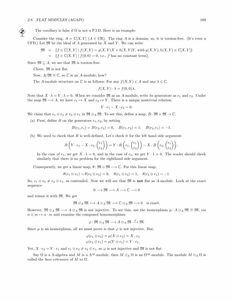
2.8. FLAT MODULES (AGAIN) 169
The corollary is false if Ω is not a P.I.D. Here is an example:
Consider the ring, A = C[X,Y ] (A ∈ CR). The ring A is a domain; so, it is torsion-free. (It’s even aUFD.) Let M be the ideal of A generated by X and Y . We can write
M = f ∈ C[X,Y ] | f(X,Y ) = g(X,Y )X + h(X,Y )Y, with g(X,Y ), h(X,Y ) ∈ C[X,Y ]= f ∈ C[X,Y ] | f(0, 0) = 0, i.e., f has no constant term.
Since M ⊆ A, we see that M is torsion-free.
Claim: M is not flat.
Now, A/M ∼= C, so C is an A-module; how?
The A-module structure on C is as follows: For any f(X,Y ) ∈ A and any λ ∈ C,
f(X,Y ) · λ = f(0, 0)λ.
Note that X · λ = Y · λ = 0. When we consider M as an A-module, write its generators as e1 and e2. Underthe map M −→ A, we have e1 7→ X and e2 7→ Y . There is a unique nontrivial relation:
Y · e1 −X · e2 = 0.
We claim that e1 ⊗ e2 6= e2 ⊗ e1 in M⊗A M. To see this, define a map, B : M×M→ C.
(a) First, define B on the generators e1, e2, by setting
B(e1, e1) = B(e2, e2) = 0, B(e1, e2) = 1, B(e2, e1) = −1.
(b) We need to check that B is well-defined. Let’s check it for the left hand side argument:
B
(Y · e1 −X · e2,
(e1
e2
))= Y ·B
(e1,
(e1
e2
))−X ·B
(e2,
(e1
e2
)).
In the case of e1, we get X · 1 = 0, and in the case of e2, we get Y · 1 = 0. The reader should checksimilarly that there is no problem for the righthand side argument.
Consequently, we get a linear map, θ : M⊗M −→ C. For this linear map,
θ(e1 ⊗ e1) = θ(e2 ⊗ e2) = 0, θ(e1 ⊗ e2) = 1, θ(e2 ⊗ e1) = −1.
So, e1 ⊗ e2 6= e2 ⊗ e1, as contended. Now we will see that M is not flat as A-module. Look at the exactsequence
0 −→M −→ A −→ C −→ 0
and tensor it with M. We get
M⊗A M −→ A⊗A M −→ C⊗A M −→ 0 is exact.
However, M ⊗A M −→ A ⊗A M is not injective. To see this, use the isomorphism µ : A ⊗A M ∼= M, viaα⊗m 7→ α ·m and examine the composed homomorphism
ϕ : M⊗A M −→ A⊗A Mµ−→M.
Since µ is an isomorphism, all we must prove is that ϕ is not injective. But,
ϕ(e1 ⊗ e2) = µ(X ⊗ e2) = X · e2
ϕ(e2 ⊗ e1) = µ(Y ⊗ e1) = Y · e1.
Yet, X · e2 = Y · e1 and e1 ⊗ e2 6= e2 ⊗ e1, so ϕ is not injective and M is not flat.
Say Ω is a Λ-algebra and M is a Λop-module, then M ⊗Λ Ω is an Ωop-module. The module M ⊗Λ Ω iscalled the base extension of M to Ω.

170 CHAPTER 2. RINGS AND MODULES
Proposition 2.70 Say M is a flat Λ-module, then its base extension, Ω⊗Λ M , is again a flat Ω-module. IfN is a flat Ω-module and Ω is a flat Λ-algebra, then N considered as Λ-module (via Λ −→ Ω), is again flatover Λ.
Proof . Assume M is flat as Λ-module. Then, we know that for any exact sequence of Λop-modules,
0 −→ N ′ −→ N −→ N ′′ −→ 0,
the sequence0 −→ N ′ ⊗Λ M −→ N ⊗Λ M is exact.
Now, take any exact sequence of Ω-modules, say
0 −→ N ′ −→ N −→ N ′′ −→ 0, (†)
it is still exact as a sequence of Λ-modules. Hence,
0 −→ N ′ ⊗Λ M −→ N ⊗Λ M is exact.
Tensoring (†) with Ω⊗Λ M over Ω, we get
N ′ ⊗Ω (Ω⊗Λ M) −→ N ⊗Ω (Ω⊗Λ M) −→ · · · . (††)
We want to show that (††) is exact on the left. But Z ⊗Ω (Ω ⊗Λ M) ∼= Z ⊗Λ M , for any Ωop-module, Z.Hence, (††) becomes
N ′ ⊗Λ M −→ N ⊗Λ M −→ · · · ,and we already observed that this sequence is exact on the left.
For the second part, take an exact sequence of Λop-modules,
0 −→M ′ −→M −→M ′′ −→ 0. (∗)
We need to show that0 −→M ′ ⊗Λ N −→M ⊗Λ N is exact.
Tensor (∗) over Λ with Ω. The resulting sequence
0 −→M ′ ⊗Λ Ω −→M ⊗Λ Ω −→ · · · (∗∗)
is still exact as Ω is flat. Tensor (∗∗) with N over Ω; again, as N is flat over Ω, we get
0 −→ (M ′ ⊗Λ Ω)⊗Ω N −→ (M ⊗Λ Ω)⊗Ω N −→ · · · is exact.
But the latter exact sequence is just
0 −→M ′ ⊗Λ N −→M ⊗Λ N −→ · · · ,
as required.
Harder question: Let P (Λ) be a property of Λ-modules. Say Ω is a Λ-algebra and M is a Λ-module.Then, we get the Ω-module, Ω⊗Λ M , the base extension of M to Ω. Suppose, Ω⊗Λ M has P (Ω). Does Mhave P (Λ)?
If so, one says that P descends in the extension Ω over Λ. This matter is a question of descent.
A more realistic question is: Given P , or a collection of interesting P ’s, for which Λ-algebras, Ω, does(do) P (Ω) descend?
Examples:

2.9. FURTHER READINGS 171
1. P1(Λ): M is a torsion-free Λ-module.
2. P2(Λ): M is a flat Λ-module.
3. P3(Λ): M is a free Λ-module.
4. P4(Λ): M is an injective Λ-module.
5. P5(Λ): M is a torsion Λ-module.
Take Λ = Z (a very good ring: commutative, P.I.D), Ω = Q (a field, a great ring), Q is flat over Z (andZ → Q). Let M = Zq (Z/2Z). (The module M is f.p.) The module M , has, none of Pj(Z) for j = 1, 2, 3, 4.On the other hand, Q ⊗Z M ∼= Q, and Q has all of Pj(Q) for j = 1, 2, 3, 4. However, P5 descends in theextension Q over Z. This follows from
Proposition 2.71 The module, M , is a torsion Z-module iff Q⊗Z M = (0).
Proof . (⇒). This has already been proved.
(⇐). First, let M be f.g. We know that there is an exact sequence
0 −→ t(M) −→M −→M/t(M) −→ 0 (†)
where t(M) is the torsion submodule of M and M/t(M) is torsion-free; hence (since M is f.g.), M/t(M) isfree. If we tensor (†) with Q, we get
Q⊗Z M −→ Q⊗Z (M/t(M)) −→ 0.
Since Q ⊗Z M = (0), by hypothesis, we get Q ⊗Z (M/t(M)) = (0). Yet, M/t(M) = qSZ where S is finite;consequently, S = ∅ and so, M/t(M) = (0), i.e., M = t(M). Therefore, M is torsion.
For an arbitrary M , we can write M = lim−→α
Mα, where Mα ranges over the f.g. submodules of M . We
have an exact sequence0 −→Mα −→M, for all α,
and Q is flat; so,0 −→ Q⊗Z Mα −→ Q⊗Z M is still exact.
But, Q⊗Z M = (0) implies Q⊗Z Mα = (0). As the Mα’s are f.g., the previous argument shows that Mα istorsion. Then, M = lim−→
α
Mα is torsion as the right limit of torsion modules is torsion.
We now go back to the question. Given the Z-module M , we assume that Q⊗ZM is torsion. Since Q isa field, Q⊗Z M = (0). Proposition 2.71 implies that M is torsion and P5 descends in the extension Q overZ.
2.9 Further Readings
Rings and modules are covered in most algebra texts, so we shall nor repeat the references given in Section1.8. Other references include Atiyah MacDonald [3], Lafon [32, 33], Eisenbud [13], Matsumura [39], Malliavin[38] and Bourbaki [8].

172 CHAPTER 2. RINGS AND MODULES

Chapter 3
Commutative Rings
3.1 Introduction
The ordinary arithmetic of the integers and simple generalizations (such as the Gaussian Integers) as wellas of analogues like the polynomial ring in one variable over a field gave rise to the study of number theoryand then to the study of commutative rings. The assumption of commutativity in multiplication makespossible a much deeper theory with more satisfying applications. Nowadays, a thorough knowledge of thisChapter is essential in order to do Algebraic Geometry and Algebraic Number Theory (and their mixture:Arithmetic Algebraic Geometry); one also needs to know the material here for Algebraic Topology. Manyof the results are direct consequences of prodding from geometry, physics and number theory. A modernproblem is to use our physical knowledge (quantum theory), our knowledge of modules and representationtheory, and the hints from the forefront of number theory to augment these results to a new and bettertheory of not necessarily commutative rings. This endeavor will probably be a big part of the twenty-firstcentury in mathematics.
3.2 Classical Localization
All rings in this chapter are commutative with unity.
Definition 3.1 Let A ∈ CR and S ⊆ A be a subset of A. We say that S is a multiplicative subset in A iff
(1) 1 ∈ S
(2) If x, y ∈ S, then xy ∈ S
(3) 0 /∈ S.
Examples:
(1) S = Gm(A) = the units of A; the idea is to abstract this case.
(2) S = α ∈ A | α is not a zero divisor in A.
(3) S = x ∈ R | x > 0 ⊆ Gm(R).
(3a) S has property (1) and (2) and is contained in Gm(A).
(4) Given f ∈ A, let S = fn | n ∈ Z, n ≥ 0 and assume that f /∈ N (A) (i.e., fn 6= 0 for all n ≥ 0).
173

174 CHAPTER 3. COMMUTATIVE RINGS
Fix a base ring, C, and look at C-algebras in CR (we get CR when C = Z). Let A and B be C-algebras,where B varies, and let S be a multiplicative subset in A. Look at
HomC−alg(A,B;S) = ϕ ∈ HomC−alg(A,B) | ϕ(S) ⊆ Gm(B).
Check that B HomC−alg(A,B;S) is a functor from C-algebras to Sets. Is it representable? This means,is there a C-algebra, S−1A, and a map (of C-algebras), h : A→ S−1A, so that
θB : HomC−alg(S−1A,B) ∼= HomC−alg(A,B;S)
functorially, where θB(ψ) = ψ h ∈ HomC−alg(A,B;S), as illustrated below:
S−1Aψ // B
A
h
OO
ψh
<<xxxxxxxxx
Proposition 3.1 The functor B HomC−alg(A,B;S) is representable. The representing object, S−1A, iscalled the fraction ring of A w.r.t. S (or the localization of A w.r.t. S). The C-algebra map, h : A→ S−1A,is the canonical map.
Proof . Look at A× S (in Sets) and form the equivalence relation, ∼, given by:
(a, s) ∼ (b, t) iff (∃u ∈ S)(u(at− sb) = 0 in A).
Writea
sfor the equivalence class of (a, s). So,
a
s=b
tiff (∃u ∈ S)(u(at− sb) = 0).
Define addition and multiplication by:
a
s+b
t=at+ sb
stand
a
s· bt
=ab
st.
Check that these operations are well defined and that S−1A is a C-algebra
(c · a
s=f(c)a
s
);1 the C-algebra
map, h : A→ S−1A, is given by h(a) =a
1.
Functorial part. Given ψ ∈ HomC−alg(S−1A,B), form ψ h taking A to B. Now, elements of S becomeunits in S−1A, because
s
1· 1
s=
1
1, the unit element of S−1A.
But, ψ maps units of S−1A to units of B, so ψh ∈ HomC−alg(A,B;S). Next, given ϕ ∈ HomC−alg(A,B;S),define
[ϕ](as
)= ϕ(s)−1ϕ(a) ∈ B.
Check
(a) The homomorphism [ϕ] : S−1A→ B is well defined.
(b) θB and ϕ 7→ [ϕ] are inverse maps.
1Here, f : C → A is the ring homomorphism making A into a C-algebra.

3.2. CLASSICAL LOCALIZATION 175
We can do the same thing with modules. Let M be an A-module and S a multiplicative set in A. Make(M × S)/ ∼, where ∼ is given by
(m, s) ∼ (n, t) iff (∃u ∈ S)(u(tm− sn) = 0 in M).
Writem
sfor the equivalence class of (m, s). Define addition and the action of A by
m
s+m′
s′=s′m+ sm′
ss′and a · m
s=am
s.
This gives the A-module, S−1M . We have the canonical map, h : M → S−1M , given by h(m) = m/1.
To discuss what this means, look at the general case of a ring homomorphism, ψ : A → B. We havetwo functors: ψ• : Mod(B) Mod(A) (the backward image functor) and ψ• : Mod(A) Mod(B) (theforward image functor). Here, ψ•(M) = M as an A-module via ψ; that means a ·m = ψ(a) ·m. The functorψ• is an exact functor. Also, the functor ψ• is given by: ψ•(M) = B ⊗AM . The forward image functor isonly right-exact, in general. These functors form a pair of adjoint functors:
HomB(ψ•(M), N) ∼= HomA(M,ψ•(N)).
Proposition 3.2 The module S−1M is, in a natural way, an S−1A-module. The map M S−1M is afunctor from Mod(A) to Mod(S−1A) and is left-adjoint to h•. That is,
HomS−1A(S−1M,N) ∼= HomA(M,h•(N)).
Consequently,S−1M ∼= S−1A⊗AM ∼= M ⊗A S−1A = h•(M).
Proof . Leta
t· ms
=am
ts, this is well-defined and makes S−1M into an S−1A-module. If ϕ : M → M in
Mod(A), the assignmentm
s7→ ϕ(m)
syields S−1ϕ : S−1M → S−1M . Check this makes M S−1M a
functor.
Say θ ∈ HomS−1A(S−1M,N), set
Θ(m) = θ(m
1
)∈ h•(N).
Now,
Θ(am) = θ(am
1
)= θ
(a1
m
1
)=a
1· θ(m
1
)=(a · θ
(m1
)in h•(N)
)= a ·Θ(m).
So, we have a map from HomS−1A(S−1M,N) to HomA(M,h•(N)) given by θ 7→ Θ. Now, sayϕ ∈ HomA(M,h•(N)); then, S−1ϕ ∈ HomS−1A(S−1M,S−1h•(N)). But, if N ∈ Mod(S−1A), thenS−1h•(N) = N , and we get the map in the opposite direction, ϕ 7→ S−1ϕ. These maps are mutuallyinverse. Each of S−1−; S−1A⊗A −; −⊗A S−1A, are left adjoint to h•; so, they are all isomorphic.
Proposition 3.3 The functor M S−1M is exact, hence, S−1A is a flat A-algebra.
Proof . Given any exact sequence M1ϕ−→ M2
ψ−→ M3, we will show that S−1M1S−1ϕ−→ S−1M2
S−1ψ−→ S−1M3
is again exact. Clearly, as M1ϕ−→M2
ψ−→M3 is exact, we have ψϕ = 0; and so, (S−1ψ)(S−1ϕ) = 0. Thisshows that Im (S−1ϕ) ⊆ Ker (S−1ψ). Say ξ ∈ S−1M2 and S−1ψ(ξ) = 0. As ξ = m/s, for some m ∈M2 andsome s ∈ S, and as S−1ψ(ξ) = ψ(m)/s = 0 in S−1M3, there is some u ∈ S with uψ(m) = 0, i.e., ψ(um) = 0.By exactness, there is some m′ ∈M1 so that um = ϕ(m′). Consider the element m′/(su); we have
S−1ϕ
(m′
su
)=ϕ(m′)
su=um
su=m
s= ξ.
Therefore, ξ ∈ Im (S−1ϕ), as required.
Examples:

176 CHAPTER 3. COMMUTATIVE RINGS
(1) S = Gm(A) or more generally, S ⊆ Gm(A). Then, S−1A = A.
(2) S = all nonzero divisors of A. Here, S−1A is a bigger ring if we are not in case (1). The ring S−1Ais called the total fraction ring of A and it is denoted Frac(A). If A is a domain, then Frac(A) isa field, the fraction field of A. For example, Frac(Z) = Q. The field, Frac(k[X1, . . . , Xn]), denotedk(X1, . . . , Xn), is the rational function field in n variables (where k is a field). If A is the ring of entire(holomorphic) functions, then Frac(A) is the field of meromorphic functions on C. If A = Hol(U), thering of holomorphic functions on an open, U ⊆ C, then Frac(A) =Mer(U) = the field of meromorphicfunctions on U .
(3) S = fn | f ∈ A (f fixed); f /∈ N (A). The ring S−1A has the special notation Af . Observe that
Af =
α
fn
∣∣∣∣ α ∈ A,n ≥ 0
,
while, in general,
Ker (h : A −→ S−1A) =α ∈ A
∣∣∣ α1
= 0
= α ∈ A | (∃u ∈ S)(uα = 0).
In cases (1) and (2), the map, h, is injective. In case (3), Ker h = α ∈ A | (∃n ≥ 0)(fnα = 0). Considerthe map A[X] −→ Af , via X 7→ 1/f (a 7→ h(a), for a ∈ A). Since aXn 7→ a/fn, our map is surjective.What is its kernel?
Consider the diagram
Af [X]X 7→1/f// Af
A[X]
h
OO
X 7→1/f // Af .
The kernel of the top arrow is: (X − 1/f). The answer to our question is now easily seen to be
P (X) ∈ A[X] | (∃r ≥ 0)(frP (X) ∈ (Xf − 1) = (Xf − 1)ec.
Here, (Xf − 1)ec is, for the moment, just a notation for the left hand side. So,
A[X]/(Xf − 1)ec ∼= Af .
Generalities on extension (e) and contraction (c).
Let ψ : A → B be a map of rings. Say A is an ideal in A. Let Ae = (the extended ideal) be the ideal ofB generated by ψ(A). If B is an ideal in B, then let Bc = (the contracted ideal) be the ideal of A given by
Bc = ψ−1(B) = x ∈ A | ψ(x) ∈ B.
Take B = S−1A. If A ⊆ A, what is Ae?
Claim: Ae =α/s | α ∈ A, s ∈ S
. Indeed, we have
Ae =
n∑
i=1
bisi
ai1
∣∣∣∣∣ ai ∈ A, bi ∈ A, si ∈ S.
Such a sum is of the form1
σ
∑ni=1 ciai, where σ = s1 · · · sn; ci ∈ A and ai ∈ A. Since A is an ideal, this sum
is of the form α/σ, where α ∈ A. We have proved part of

3.2. CLASSICAL LOCALIZATION 177
Proposition 3.4 For any commutative ring, A, and any multiplicative subset, S, of A we have:
(1) Gm(S−1A) = α/s | (∃b ∈ A)(bα ∈ S).
(2) If A ⊆ A then Ae = α/s | α ∈ A, s ∈ S.
(3) Ae = (1) = S−1A iff A ∩ S 6= ∅.
Proof . (1) We have α/s ∈ Gm(S−1A) iff there is some β/t withβα
ts= 1 =
1
1iff (∃u ∈ S)((uβ)α = ust).
But, ust ∈ S; so, if we set b = uβ, we get bα ∈ S. The converse is clear.
(2) Already done.
(3) We have Ae = (1) iff some element of Ae is a unit iff α/s is a unit for some α ∈ A iff there is someb ∈ A with bα ∈ S. But, α ∈ A, so bα ∈ A, yet bα ∈ S; so, A ∩ S 6= ∅. Conversely, if A ∩ S 6= ∅, thens/1 | s ∈ S ∩ Ae 6= ∅. Consequently, Ae has a unit in it, and so, Ae = (1).
Say A ⊆ A, when is A contracted? First an easier question: What is Aec?
Note: for all v ∈ A, we have A ⊆ (v −→ A) (this only uses the fact that A is a two-sided ideal).
Claim: (v −→ A) = A iff v is not a zero divisor modA, i.e., v ∈ A/A is not a zero divisor. (Terminology:v is regular w.r.t, A).
We have (v −→ A) = A iff (v −→ A) ⊆ A iff for every ξ ∈ A, when ξv ∈ A, then ξ ∈ A. Reading thismod A, we find the above statement is equivalent to
(∀ξ ∈ A/A)(ξv = 0 =⇒ ξ = 0),
which holds iff v is not a zero divisor in A/A.
Going back to the question: What is Aec?, we have ξ ∈ Aec iff h(ξ) ∈ Ae iff h(ξ) = α/s, for some α ∈ Aand some s ∈ S, iff ξ/1 = α/s iff there is some u ∈ S so that u(ξs− α) = 0, i.e. uξs = uα ∈ A. As us ∈ S,this implies that there is some v ∈ S with vξ ∈ A. Conversely, if vξ ∈ A for some v ∈ S, then
v
1
ξ
1∈ Ae =⇒ 1
v
v
1
ξ
1∈ Ae =⇒ ξ
1∈ Ae =⇒ h(ξ) ∈ Ae,
and so, ξ ∈ Aec. Therefore,
Aec = ξ | (∃v ∈ S)(vξ ∈ A)= ξ | (∃v ∈ S)(ξ ∈ (v −→ A))=
⋃
v∈S(v −→ A).
Now, A = (1 −→ A) ⊆ ⋃s∈S(s −→ A) = Aec.
When is A contracted, i.e., when is it of the form A = Bc, for some B ⊆ S−1A?
Of course, if A = Aec, then B = Ae will do. In fact, we shall prove that A = Bc for some B ⊆ S−1A iffA = Aec. First, we claim that B = Bce for every B ⊆ S−1A; that is, every ideal, B, of S−1A is an extendedideal. For, any ξ in B is of the form ξ = α/s, for some α ∈ A and some s ∈ S. But, sξ ∈ B, too, and so,α/1 ∈ B, which implies that α ∈ Bc. Consequently, ξ = α/s ∈ Bce. Conversely, if ξ ∈ Bce, then ξ = β/t,with β ∈ Bc; it follows that ξ = (1/t)(β/1) ∈ B, and so, B = Bce.
But now, A = Bc implies that Ae = Bce = B; so, Aec = Bc = A. These remarks prove most of the
Proposition 3.5 If A ∈ CR and S is a multiplicative system in A, then

178 CHAPTER 3. COMMUTATIVE RINGS
(1) An ideal, A, of A is contracted iff A = Aec iff every element of S is regular for A.
(2) Every ideal, B ⊆ S−1A, is extended.
(3) The map, A 7→ Ae, is a one-to-one inclusion-preserving correspondence between all the contracted idealsof A and all ideals of S−1A.
(4) If A is noetherian, then S−1A is noetherian.
Proof . (1) We proved earlier that Aec =⋃v∈S(v −→ A) and we know that (v −→ A) = A iff v is regular for
A. So, (1) is now clear.
(2) This has already been proved.
(3) Assume that A and A have the same extension and both are contracted. Then, by (1) A = Aec and
A = Aec, and since, by hypothesis Ae = Ae, we get A = A. It is also clear that if A ⊆ A, then Ae ⊆ Ae.
(4) (DX) from (1), (2), (3).
The same argument shows the corresponding proposition for modules.
Proposition 3.6 If A ∈ CR and S is a multiplicative system in A, for any module, M ∈Mod(A),
(1) A submodule, N , of M is contracted iff it is equal to its S-saturation. The S-saturation of N is thesubmodule given by
ξ ∈M | (∃v ∈ S)(vξ ∈ N) =⋃
v∈S(v −→ N),
where (v −→ N) = ξ ∈M | vξ ∈ N.
(2) Every submodule of S−1M is extended, i.e., has the form S−1N , for some submodule, N , of M .
(3) The map, N 7→ S−1N , is a one-to-one inclusion-preserving correspondence between all the S-saturatedsubmodules of M and all submodules of S−1M .
(4) If M is a noetherian module, then S−1M is a noetherian module.
Proposition 3.7 Say A ∈ CR and S is a multiplicative system in A. For any ideal, A ⊆ A, we have
(a) The image, S, of S in A/A, is a multiplicative subset provided that S ∩ A = ∅.
(b) S−1A/Ae −→ S−1
(A/A).
Proof . (a) This is trivial.
(b) We have A −→ A/A −→ S−1
(A/A). The elements of S become units in S−1
(A/A). By the universal
mapping property, we have the map S−1A −→ S−1
(A/A). This map is a/s 7→ a/s; so, it is surjective. We
have a/s = 0 in S−1
(A/A) iff there is some u ∈ S so that u a = 0 iff a/1 ∈ Ae iff a/s ∈ Ae. Therefore, the
kernel of our map is Ae, and so, S−1A/Ae −→ S−1
(A/A).

3.3. PRIME AND MAXIMAL IDEALS 179
3.3 Prime and Maximal Ideals
Recall that an ideal, p, of A ∈ CR is a prime ideal iff p 6= (1) and for all a, b ∈ A, if ab ∈ p, then one of a ∈ por b ∈ p holds.
Proposition 3.8 Given a commutative ring, A, for any ideal, A ⊆ A, the following are equivalent:
(1) The ideal, A, is a prime ideal.
(2) The ring A/A is an integral domain.
(3) The set S = A− A = the complement of A is a multiplicative subset of A.
(4) If B and B are two ideals of A and if BB ⊆ A, then one of B ⊆ A or B ⊆ A holds.
(5) There is a ring, B, a homomorphism, ϕ : A→ B and a maximal ideal, m, of B, so that ϕ−1(m) = A.
(6) There is a multiplicative set, S ⊆ A, so that
(i) A ∩ S = ∅ and
(ii) A is maximal among the ideals having (i).
Proof . Equivalence of (1)–(4) is known and clear. Now, the inverse image of a prime ideal is always a primeideal (DX). Every maximal ideal is prime, so it follows that (5) ⇒ (1). Moreover, (1) implies (6) becausetake S = A− p. This is a multiplicative set by (3) and (6) follows tautologically.
(1) ⇒ (5). Given a prime, A, let S = A − A, a multiplicative set by (3) and let B = S−1A and ϕ = h.
We claim that Ae is a maximal ideal of S−1A. This is because S−1A/Ae −→ S−1
(A/A), but A/A is an
integral domain and S = nonzero elements of A/A. Consequently, S−1
(A/A) = Frac(A/A) is a field; so, Ae
is a maximal ideal. Now, h−1(Ae) = Aec =⋃v∈S(v −→ A). Now, ξ ∈ (v −→ A) iff vξ ∈ A, where v /∈ A.
But, A is prime, so ξ ∈ A. Therefore, (v −→ A) = A, for all v ∈ S; and so, Aec = h−1(Ae) = A and (5)follows.
(6)⇒ (1). Given any a, b /∈ A, we must show that ab /∈ A. The hypotheses imply that A + (a) > A andA + (b) > A, and by (6) (i) and (ii), we have (A + (a)) ∩ S 6= ∅ and (A + (b)) ∩ S 6= ∅. So, there are somes, t ∈ S, where s = α+ ρa, t = β + σb, with α, β ∈ A, ρ, σ ∈ A. Since st ∈ S, it follows that
αβ + ρaβ + σbα+ ρσ(ab) ∈ S.
If ab ∈ A, then st ∈ A ∩ S, a contradiction. Therefore, ab /∈ A.
Corollary 3.9 Given any multiplicative set, S, in A, there exists a prime ideal, p, so that p ∩ S = ∅.
Proof . Look at S = A | A an ideal and A ∩ S = ∅. We have (0) ∈ S, partially order S by inclusion andcheck that S is inductive. By Zorn’s lemma, S has some maximal element, p. By (6), the ideal p is prime.
Notation: If S = A − p, where p is a prime ideal, write Ap instead of S−1A; the ring Ap is called thelocalization of A at p. Recall that a local ring is a ring that has a unique maximal ideal.
Corollary 3.10 For any prime ideal, p, in A, the ring Ap is always a local ring and its maximal ideal isjust pe.
Proof . Say A is an ideal of A. Ideals of Ap = S−1A are extended ideals, i.e., they are of the form Ae. Wehave Ae = (1) iff A ∩ S 6= ∅ iff A 6⊆ p. Thus, Ae is a proper ideal iff A ⊆ p; the latter implies that Ae ⊆ pe.So, pe is the maximal ideal of Ap, as contended.
Remark: We have pec = p. We saw this above in the proof that (1)⇒ (5).

180 CHAPTER 3. COMMUTATIVE RINGS
Proposition 3.11 Let A ∈ CR be a commutative ring, S be a multiplicative set in A and let P be a primeideal of A. Then,
(1) The ideal Pe is a prime ideal of S−1A iff Pe 6= (1) iff P ∩ S = ∅.
(2) Every prime ideal of S−1A has the form Pe, for some prime ideal, P, of A.
(3) There is a one-to-one, inclusion-preserving, correspondence between the prime ideals of S−1A and theprime ideals, P, of A for which P ∩ S = ∅.
When S = A− p for some prime, p, of A, we have
(1′) The ideal Pe is a prime of Ap iff P is a prime in A and P ⊆ p.
(2′) Every prime ideal of Ap is Pe, for some prime, P, of A with P ⊆ p.
(3′) There is a one-to-one, inclusion-preserving, correspondence between all primes of Ap and theprimes of A contained in p.
Proof . (1) We know that Pe 6= (1) iff P ∩ S = ∅. By definition, a prime ideal is never equal to (1), so, allwe must show is: If P is prime in A, then Pe is prime in S−1A (of course, Pe 6= (1)). Say (α/s)(β/t) ∈ Pe.Then, (αβ)/1 ∈ Pe, and so, αβ ∈ Pec. But, Pec =
⋃v∈S(v −→ P) and ξ ∈ (v −→ P) iff vξ ∈ P; moreover,
v /∈ P since P ∩ S = ∅, so, ξ ∈ P. Therefore, Pec = P, and so, αβ ∈ P. Since P is prime, either α ∈ P orβ ∈ P; it follows that either α/s ∈ Pe or β/t ∈ Pe.
(2) If q is a prime in S−1A, then q = qce and qc is a prime, as qc = h−1(q). Take P = qc to satisfy (2).Conversely, Pe is prime iff P ∩ S = ∅.
(3) follows from (1) and (2) and previous work.
Finally, (1′), (2′) and (3′) are special cases of (1), (2) and (3), respectively.
Definition 3.2 If p is a prime ideal of A ∈ CR, look at chains of prime ideals
p = p0 > p1 > · · · > pn,
where each pj is prime ideal of A. Call n the length of this chain and define the height of p by
ht(p) = suplength of all chains p = p0 > p1 > · · · > pn.
Observe that ht(p) might be infinite. Since there is a one-to-one inclusion-preserving correspondencebetween the set of all primes, P, contained in p and the set of all prime ideals of Ap, we get
ht(p) = ht(maximal ideal of Ap).
Definition 3.3 The Krull dimension of a commutative ring, A, denoted dim(A), is the supremum of theset ht(m) | m is a maximal ideal of A.
Hence, we see that ht(p) = dim(Ap), and
dim(A) = supdim(Am) | m is a maximal ideal of A.
Examples.
(1) Say dim(A) = 0. This holds iff every prime ideal is maximal iff every maximal ideal is a minimalprime ideal. An example is a field, or Z/nZ.

3.3. PRIME AND MAXIMAL IDEALS 181
(2) dim(A) = 1. Here, A = a P.I.D. will do. For example, Z, Z[i], Q[T ], more generally, k[T ], for anyfield, k. Also, Z[
√−5], a non-P.I.D., has dimension 1.
(3) C[T1, . . . , Tn] has dimension n (this is not obvious, try it!) Given a commutative ring, A, for appli-
cations to algebraic geometry and number theory, it is useful to introduce two important sets, SpecA andMaxA, and to make these sets into topological spaces. Let
SpecA = p | p is a prime ideal of AMaxA = m | m is a maximal ideal of A.
The set, X = SpecA, is given a topology (the Zariski topology or spectral topology) for which a basis ofopen sets consists of the sets
Xf = p ∈ SpecA | f /∈ p (f ∈ A),
and MaxA ⊆ SpecA is given the relative topology.
Remarks:
(1) Xfn = Xf , for all n ≥ 1. This is because fn /∈ p iff f /∈ p, as p is prime.
(2) Xfg = Xf ∩Xg. This is because p ∈ Xfg iff fg /∈ p iff (f /∈ p) and (g /∈ p).
(3) Xf = SpecA = X iff f /∈ p, for every prime p iff f ∈ Gm(A) iff Xf = X1.
(4) Xf = ∅ iff f ∈ p, for all primes, p.
The open sets in X = SpecA are just the sets of the form⋃f∈T Xf , for any subset, T , of A. So, a set,
C, is closed in X iff it is of the form C =⋂T X
cf , where
Xcf = p ∈ SpecA | p /∈ Xf = p ∈ SpecA | f ∈ p = p ∈ SpecA | (f) ⊆ p.
Thus, p ∈ C iff the ideal generated by the set T is contained in p. This suggests the following definition: Forany ideal, A, in A, let
V (A) = p ∈ SpecA | p ⊇ Abe the variety defined by A. Then, we have
V (A) =⋂
f∈A
Xcf =
⋂Xc
f | f is part of a generating set for A.
The dual properties to (1)–(4) are:
(1′) V (A ∩B) = V (AB) = V (A) ∪ V (B)
(2′) V (∑α Aα) =
⋂α V (Aα) (
∑α Aα = the ideal generated by the Aα’s).
(3′) V (A) = ∅ iff A = (1).
(4′) V (A) = X = SpecA iff (∀p ∈ SpecA)(A ⊆ p).
From now on, when we refer to SpecA and MaxA, we mean these as topological spaces.
To give a more informative criterion for (4) and (4′), we need to study N (A) = the nilradical of A,defined by
N (A) = x ∈ A | xn = 0, for some integer n > 0.

182 CHAPTER 3. COMMUTATIVE RINGS
This is an ideal of A. Indeed, if x ∈ N (A) and y ∈ A, since A is commutative, we have (yx)n = ynxn = 0.Also, if x, y ∈ N (A), then there is some integer n ≥ 0 so that xn = yn = 0, and by the binomial formula,
(x± y)2n =
2n∑
j=0
(2n
j
)xj(±1)2n−jy2n−j = 0,
since y2n−j = 0 if j ≤ n and xj = 0 if j ≥ n. Therefore, x± y ∈ N (A) and N (A) is an ideal.
More generally, if A is an ideal, the radical of A, denoted√A, is
√A = x ∈ A | (∃n ≥ 0)(xn ∈ A).
It is easy to check that√A is an ideal and that A ⊆
√A. Note:
√(0) = N (A).
That√A is an ideal can also be seen as follows: Consider the projection map, A
bar−→ A/A, and look atN (A/A). Then,
√A is the inverse image of N (A/A) under bar, and so,
√A is an ideal. Furthermore, by
the first homomorphism theorem,A/√A ∼= (A/A)/N (A/A).
Observe that A/N (A) is a ring without nonzero nilpotent elements. Such a ring is called a reduced ring andA/N (A) is reduced. We write Ared for A/N (A). Note: (A/A)red = A/
√A. For example,
(Z/pnZ)red = Z/pZ, for any prime p.
The following facts are easy to prove (DX):
(a)√√
A =√A.
(b)√A ∩B =
√A ∩√B.
(c) If Ak ⊆ B, for some k ≥ 1, then√A ⊆
√B.
There is another radical, the Jacobson radical , J (A), given by
J (A) =⋂
m∈Max(A)
m.
Proposition 3.12 For any ring, A ∈ CR, we have
(1) x /∈ Gm(A) iff there is some maximal ideal, m, so that x ∈ m.
(2) If x ∈ J (A), then 1 + x ∈ Gm(A).
(3) N (A) =⋂
p∈SpecA p; hence N (A) ⊆ J (A).
Proof . (1) is clear (use Zorn’s lemma).
(2) Assume (1 + x) /∈ Gm(A). By (1), there is some m ∈ MaxA, so that 1 + x ∈ m. So, x /∈ m (else,1 ∈ m, a contradiction). As J (A) is contained in every maximal ideal, we get x /∈ J (A).
(3) Suppose x ∈ N (A); then, xn = 0, for some n ≥ 0. Consequently, xn ∈ p, for every prime p; so,x ∈ p, as p is prime. Conversely, assume x ∈ ⋂p∈Spec(A) p. Look at the set S = xn | n ≥ 0. Were S a
multiplicative set, then there would be some prime ideal, p, with p ∩ S = ∅. As x ∈ p, this is impossible.Therefore, S is not a multiplicative set, which happens iff x is nilpotent.
Now, we can give the criteria for (4) and (4′).
(4) Xf = ∅ iff f ∈ N (A).

3.3. PRIME AND MAXIMAL IDEALS 183
(4′) V (A) = X = SpecA iff A ⊆ N (A).
Corollary 3.13 Given any ideal, A,
√A =
⋂p ∈ SpecA | p ⊇ A =
⋂p ∈ SpecA | p ∈ V (A).
Proof . There is a one-to-one correspondence between the set of prime ideals, p, containing A and the set ofprime ideals, p, in A/A. So,
⋂p | p ⊇ A is the inverse image of N (A/A), but this inverse image is√A.
The minimal elements among primes, p, such that p ⊇ A are called the isolated primes of A. Therefore,
√A =
⋂p ∈ SpecA | p is an isolated prime of A.
Proposition 3.14 The space X = SpecA is always quasi-compact (i.e., compact but not necessarily Haus-dorff).
Proof . Say⋃α Uα = X is an open cover of X. Each open Uα has the form Uα =
⋃β Xf
(α)β
. Therefore, we
get an open cover⋃α,β Xf
(α)β
= X. If we prove that this cover has a finite subcover, we are done (DX). The
hypothesis implies that⋂α,β X
c
f(α)β
= ∅. However the left hand side is V ((f(α)β )) and so (f
(α)β ) = (1), by
previous work. We find
1 = cα1,β1f
(α1)β1
+ · · ·+ cαs,βsf(αs)βs
, for some cαj ,βj ∈ A.
Thus, already, (f(αj)βj
)sj=1 = (1), and so,⋂sj=1X
c
f(αj)
βj
= ∅. Thus,⋃sj=1Xf
(αj)
βj
= X, a finite cover.
Remark: The space, SpecA, is almost never Hausdorff. For example,Spec(Z) = (0), (2), (3), (5), (7), (11), . . ., and (0) is dense in Spec(Z), i.e., every open set contains (0).
Another geometric example of SpecA and MaxA is this:
Proposition 3.15 Let X be a compact, Hausdorff space and write A = C(X) (the ring of real-valued (orcomplex-valued) continuous functions on X). For each x ∈ X, write mx = f ∈ A | f(x) = 0. Then
(1) Each mx is a maximal ideal of A and
(2) The map x 7→ mx is a bijection of X with MaxA. (In fact, x 7→ mx is a homeomorphism).
Proof . Note that the map f 7→ f(x) is a homomorphism of C(X) onto R (resp. C). Its kernel is mx, and so,mx is maximal. By Urysohn’s lemma, if x 6= y, there is some continuous function, f ∈ A, so that f(x) = 0and f(y) = 1. Thus, f ∈ mx and f /∈ my; it follows that mx 6= my; so, our map is an injection (of sets).Take any m in MaxA. Say, m 6= mx for all x ∈ X. Given x ∈ X, since m 6= mx, there is some fx ∈ m andfx /∈ mx, Therefore, fx(x) 6= 0. Since f is continuous, there is some open subset, Ux, with x ∈ Ux, andf Ux 6= 0. Then, the family Ux is an open cover of X, and by compactness, it contains a finite subcover,say Uxjtj=1. We have a function, fxj ∈ m, for each j = 1, . . . , t. Let
F =
t∑
j=1
f2xj
(F =
t∑
j=1
|fxj |2, in the complex case).
Clearly, F ≥ 0. Pick any ξ ∈ X. Then, there is some j, with 1 ≤ j ≤ t, so that ξ ∈ Uxj , and so, fxj (ξ) 6= 0.It follows that F (ξ) > 0. Thus, F is never zero on X; consequently, 1/F ∈ A. But now, F is a unitand yet, F ∈ m, a contradiction. Therefore, the map x 7→ mx is surjective. We leave the fact that it is ahomeomorphism as a (DX).
Here are some useful lemmas on primes.

184 CHAPTER 3. COMMUTATIVE RINGS
Lemma 3.16 If p is a prime of A and A1, . . . ,At are some given ideals, then p ⊇ ⋂tj=1 Aj iff p ⊇ Aj, forsome j.
Proof . (⇐). This is a tautology.
(⇒). Observe that p ⊇ ⋂tj=1 Aj ⊇∏tj=1 Aj , and since p is prime, we must have p ⊇ Aj , for some j.
Lemma 3.17 (Prime avoidance lemma) Let A be an ideal and let p1, . . . , pt be some prime ideals. IfA ⊆ ⋃tj=1 pj, then A ⊆ pj, for some j. (The lemma says that if A avoids all the pj, in the sense that A 6⊆ pj,
then it avoids⋃tj=1 pj).
Proof . We proceed by induction on t. The case t = 1 is obvious. Assume the induction hypothesis fort < n. Given n prime ideals, p1, . . . , pn, by the induction hypothesis, we may assume that A 6⊆ ⋃j 6=i pj , for
i = 1, . . . , n. Since, by hypothesis, A ⊆ ⋃nj=1 pj , for every i = 1, . . . , n, there is some xi ∈ A with
xi ∈ pi and xi /∈ pj , for all j 6= i. (†)Let k be given and form
yk = x1 · · ·xk−1xkxk+1 · · ·xn,where, as usual, the hat over xk means that xk is omitted. Then, yk ∈ pi, for all i 6= k. We claim thatyk /∈ pk. Indeed, were it not the case, then we would have yk = x1 · · · xk · · ·xn ∈ pk; since pk is prime, therewould be some xj ∈ pk for some j 6= k, a contradiction of (†).
Of course, yk ∈ A, for all k. Now, take a = y1 + · · ·+ yn.
Claim. a /∈ ⋃nj=1 pj .
Suppose that a ∈ pk, for some k. We can write
a = yk +∑
j 6=k
yj ∈ pk, (∗)
and since we proved that yj ∈ pk for all j 6= k, the fact that a ∈ pk implies that yk ∈ pk, a contradiction.
Lemma 3.18 Say p1, . . . , pn are prime ideals in A, then S = A−⋃nj=1 pj is a multiplicative subset of A.
Proof . We have 0 /∈ S and 1 ∈ S. Suppose that s, t ∈ S and st /∈ S. Then, st ∈ ⋃nj=1 pj , and so, st ∈ pj forsome j; as pj is prime, either s ∈ pj or t ∈ pj , a contradiction.
Now, I.S. Cohen (1950) showed that noetherian-ness of a ring is controlled by its prime ideals.
Lemma 3.19 (Cohen, 1950) If A is an ideal in a commutative ring, A, and if b is an element of A forwhich A + (b) is f.g. and (b −→ A) is also f.g., then A is f.g.
Proof . Say A + (b) is generated by β1, . . . , βt. Each βj is of the form aj + ρjb, for some aj ∈ A and someρj ∈ A. So, the elements a1, . . . , at and b generate A+ (b). Let c1, . . . , cs generate (b −→ A). Then, cjb ∈ A,for j = 1, . . . , s.
We claim that the elements a1, . . . , at, c1b, . . . , csb generate A.
Pick α ∈ A, then α ∈ A + (b), and so, α =∑tj=1 vjaj + ρb, with aj as above, for j = 1, . . . , t. But,
ρb = α−t∑
j=1
vjaj ∈ A,
and so, ρ ∈ (b −→ A). Consequently, we can write ρ =∑sj=1 ujcj , as the cj ’s generate (b −→ A). It follows
that
α =
t∑
j=1
vjaj +
s∑
j=1
uj(cjb),
as contended.

3.3. PRIME AND MAXIMAL IDEALS 185
Proposition 3.20 Let A be a commutative ring, then the following are equivalent:
(1) A is noetherian (A has the ACC).
(2) Every ideal of A is f.g.
(3) A has the maximal condition on ideals.
(4) A has the ACC on f.g. ideals.
(5) (I.S. Cohen, 1950) Every prime ideal of A is f.g.
Proof . We already proved the equivalence (1)–(3) (c.f. Proposition 2.9). Obviously, (1) implies (4) and (2)implies (5).
(4)⇒ (1). SupposeA1 < A2 < A3 < · · ·
is a strictly ascending chain of ideals of A. By the axiom of choice, we can find a tuple, (aj)∞j=1, of elements
in A so that aj ∈ Aj and aj /∈ Aj−1. Look at the ascending chain
(a1) ⊆ (a1, a2) ⊆ (a1, a2, a3) ⊆ · · · ⊆ (a1, . . . , an) ⊆ · · · .This is a strictly ascending sequence, by the choice of the aj ’s, a contradiction.
(5) ⇒ (2). Take F = A an ideal of A | A is not f.g. and partially order F by inclusion. If F is notempty, it is inductive (DX). By Zorn’s lemma, F has a some maximal element, A. Since A ∈ F , it is not f.g.and by (5), the ideal A is not prime. So, there exist a, b ∈ A with a, b /∈ A and yet, ab ∈ A. Since b /∈ A, wehave A+ (b) > A. Now, a ∈ (b −→ A) (since ab ∈ A), yet, a /∈ A, and so, (b −→ A) > A. As A is maximal inF , it follows that both A+ (b) and (b −→ A) are f.g. By Cohen’s lemma, the ideal A is f.g., a contradiction.Therefore, F = ∅, and (2) holds.
We now move back to modules. Given an A-module, M , we make the definition
Definition 3.4 The support of an A-module, M , denoted Supp(M) is that subset of SpecA given by
Supp(M) = p ∈ SpecA |Mp 6= (0).Proposition 3.21 If M is an A-module, then
Supp(M) ⊆ V ((M −→ (0))) = V (Ann(M)).
If M is f.g., thenSupp(M) = V ((M −→ (0))).
So, the support of a f.g. module is closed in SpecA.
Proof . Pick p in Supp(M), i.e., Mp 6= (0). We need to show that p ∈ V ((M −→ (0))), i.e., p ⊇ (M −→ (0)).We will show that if p 6⊇ (M −→ (0)) then Mp = (0). But, p 6⊇ (M −→ (0)) implies that there is some s /∈ pwith s ∈ (M −→ (0)). In Mp,
s
1
m
t=sm
t= 0, as s kills M
But, s/1 is a unit in Ap, and so, m/t = 0 already, and Mp = (0).
Now, say M is f.g. with m1, . . . ,mt as generators. Pick p ∈ V ((M −→ (0))), we need to show thatp ∈ Supp(M). This means, if p ⊇ Ann(M), then Mp 6= (0). We will prove that if Mp = (0), thenp 6⊇ Ann(M).
If Mp = (0), then m/1 = 0. So, there is some s = s(m) ∈ S with sm = 0 in M . If we repeat this processfor each of the m1, . . . ,mt that generate M , we get s1, . . . , st ∈ S such that sjmj = 0, for j = 1, . . . , t. Writeσ = s1 · · · st ∈ S. We get σmj = 0 for all j = 1, . . . , t; so, σ ∈ Ann(M). But, σ ∈ S implies that σ /∈ p;consequently, p 6⊇ Ann(M).

186 CHAPTER 3. COMMUTATIVE RINGS
Proposition 3.22 Say M is an A-module (where A ∈ CR). Then, the following are equivalent:
(1) M = (0).
(2) Supp(M) = ∅.
(2a) Mp = (0), for all p ∈ SpecA.
(3) Supp(M) ∩MaxA = ∅.
(3a) Mm = (0), for all m ∈ MaxA.
Proof . The implications (2) ⇔ (2a) and (3) ⇔ (3a) are obvious. Similarly, (1) ⇒ (2) and (2) ⇒ (3)are trivial. So, we need to show (3) ⇒ (1). Let us first assume that M is f.g., Then, we know thatSupp(M) = V ((M −→ (0))). The hypothesis (3) implies that m ⊇ (M −→ (0)) for no maximal ideal, m.This implies that (M −→ (0)) = (1), the unit ideal. Consequently, 1 ∈ (M −→ (0)), and so, M = (0).
Let us now consider the case where M is not f.g. We can write M = lim−→α
Mα, where the Mα’s range over
the f.g. submodules of M . Now, Mα ⊆M and localization being exact, (Mα)m ⊆Mm; so, (Mα)m = (0) forall m ∈ MaxA. By the f.g. case, we get Mα = (0) for all α, and thus, M = (0).
Remark: The implication (3) ⇒ (1) can also be proved without using right limits. Here is the proof. Assume
M 6= (0). Then, there is some m ∈ M with m 6= 0, and let Ann(m) = a ∈ A | am = 0; we have Ann(m) 6= (1);
so, Ann(m) ⊆ m, for some maximal ideal, m. Consider m/1 ∈ Mm. Since Mm = (0), we have λm = 0, for some
λ ∈ A−m; thus, λ ∈ Ann(m), and yet λ /∈ m ⊇ Ann(m), a contradiction. Therefore, M = (0).
Corollary 3.23 If M ′ϕ−→ M
ψ−→ M ′′ is a given sequence of modules and maps, then it is exact iff for allp ∈ SpecA, the sequence M ′p −→Mp −→M ′′p is exact iff for all m ∈ MaxA, the sequenceM ′m −→Mm −→M ′′m is exact.
Proof . (⇒). This direction is trivial as localization is an exact functor.
Observe that we need only assume that the sequence M ′m −→ Mm −→ M ′′m is exact for all m ∈ MaxA.Then, (ψ ϕ)m = ψm ϕm = 0; so if N is the image of the map ψ ϕ, we find Nm = (0), for all m ∈ MaxA.By Proposition 3.22, we get N = (0), and thus ψ ϕ = 0.
Let H = Ker ψ/Im ϕ. The same argument (using exactness of localization) shows thatHm∼= (Ker ψ)m/(Im ϕ)m = (0). Again, Proposition 3.22 implies that H = (0) and Ker ψ = Im ϕ, as
contended.
The statement is not that a whole family of local morphisms comes from a global morphism, rather wemust have the global morphisms and then exactness is a local property.
Local Terminology: If P is property of A-modules (or morphisms), then a module (or morphism) islocally P iff for every p ∈ SpecA, the module Mp has P as Ap-module.2
Examples: Locally f.g., locally f.p., locally flat, locally exact, locally free, locally zero. etc.
Sometimes, you get a global result from an everywhere local result.
Proposition 3.24 (Local flatness criterion) Say M is an A-module (where A ∈ CR). Then, the followingare equivalent:
(1) M is flat over A.
2In reality, this ought to be called “pointwise P”.

3.3. PRIME AND MAXIMAL IDEALS 187
(2) M is locally flat.
(2a) For every p ∈ SpecA, the module Mp is flat over A.
(3) For every m ∈ MaxA, the module Mm is flat over Am.
(3a) For every m ∈ MaxA, the module Mm is flat over A.
Proof . The implications (1) ⇒ (2) and (2) ⇒ (3) hold, the first by base extension and the second becauseit is a tautology. We shall prove that (3)⇒ (1) (and along the way, (3)⇐⇒ (3a) and hence, (2)⇐⇒ (2a)).Assume 0 −→ N ′ −→ N is exact. Tensoring with M , we get N ′ ⊗A M −→ N ⊗A M . Consider the exactsequence
0 −→ K −→ N ′ ⊗AM −→ N ⊗AM,
where K = Ker (N ′ ⊗AM −→ N ⊗AM). By localizing at m, we get the exact sequence
0 −→ K ⊗A Am −→ (N ′ ⊗AM)⊗A Am −→ (N ⊗AM)⊗A Am. (∗)
It follows that the sequence
0 −→ Km −→ N ′ ⊗AMm −→ N ⊗AMm is exact. (∗∗)
Now, for any module, L,
(L⊗AM)⊗A Am∼= (L⊗A Am)⊗Am
(M ⊗Am) ∼= Lm ⊗AmMm,
and so, the sequence
0 −→ Km −→ N ′m ⊗AmMm −→ Nm ⊗Am
Mm is also exact. (†)
Since, the sequence 0 −→ N ′m −→ Nm is exact and
(a) Mm is Am-flat; we find Km = (0).
(b) Mm is A-flat; we find Km = (0), again.
But, the above holds for all m ∈ MaxA, and thus, K = (0), as required.
This method amounts to studying modules over the Ap’s and the latter are local rings, where mattersare usually easier. The basic fact is Nakayama’s lemma.
Lemma 3.25 (Nakayama’s lemma) Say A is a commutative ring and J (A) is its Jacobson radical. Supposethat M is a f.g. A-module and that J (A)M = M . Then, M = (0). That is, if M ⊗A (A/J (A)) = (0), thenM = (0) (recall that M ⊗A (A/J (A)) ∼= M/(J (A)M)).
Proof . Pick a generating set for M of least cardinality. If M 6= (0), this set is nonempty. Write m1, . . . ,mt
for these generators. As M = J (A)M , we can express mt ∈ M as mt =∑tj=1 αjmj , where αj ∈ J (A).
Consequently,
(1− αt)mt =
t−1∑
j=1
αjmj .
Now, 1−αt ∈ Gm(A), since αt ∈ J (A). Therefore, mt =∑t−1j=1 αj(1−αt)−1mj , contradicting the minimality
of t.
Corollary 3.26 (Classical Nakayama) Say A is a local ring and mA is its maximal ideal. Suppose that Mis a f.g. A-module and that mAM = M . Then, M = (0).

188 CHAPTER 3. COMMUTATIVE RINGS
Corollary 3.27 On the category of f.g. modules, A/J (A) is a faithful module. This means ifM ⊗A (A/J (A)) = (0), then M = (0). (In the local ring case, if M ⊗A κ(A) = (0), then M = (0), withκ(A) = A/mA.)
Corollary 3.28 Let M be an f.g. A-module and say m1, . . . ,mt ∈M have residues m1, . . . ,mt inM = M ⊗A (A/J (A)) ∼= M/(J (A)M) which generate M . Then, m1, . . . ,mt generate M .
Proof . Let N be the submodule of M generated by m1, . . . ,mt. Look at M/N = M/N . Since M is f.g.,M/N is f.g. and M/N = M/N = (0). By Corollary 3.27, we get M/N = (0), i.e., M = N .
Corollary 3.29 Let M be an f.g. A-module and let N be a submodule for which N + J (A)M = M . Then,N = M .
Proof . The hypothesis means M = N ; so, M/N = (0). We conclude using Corollary 3.27, again.
Corollary 3.30 Let A be a local ring and M be a f.g. A-module. Write t for the minimal cardinality of aset of generators for M . Then
(1) A set of elements m1, . . . ,mr generate M iff m1, . . . ,mr span the vector space M ⊗A κ(A).
(2) Every set of generators of M contains a subset generating M with exactly t elements.
The integer t is equal to dimκ(A)(M ⊗A κ(A)).
Proof . (1) The implication (⇒) is clear and the implication (⇐) follows from Corollary 3.28.
(2) For vector spaces, each spanning set contains a basis; this implies that each generating set of Mcontains elements which pass to a basis. So, t ≥ d = dimκ(A)(M ⊗A κ(A)). As any basis of a vector spacespans the vector space, Corollary 3.28 shows that M has a generating set of d elements, and so, t ≤ d.Therefore, t = d.
Proposition 3.31 Let A be a local ring and M be an A-module. Assume one of
(a) A is noetherian and M is f.g.
(b) M is f.p.
Then, the following are equivalent:
(1) M is free over A.
(2) M is projective over A.
(3) M is faithfully flat over A.
(4) M is flat over A.
Proof . The implications (1) ⇒ (2), (2) ⇒ (4) and (1) ⇒ (3), are already known (c.f. Remark (1) afterDefinition 2.4 for (1)⇒ (2) and c.f. Proposition 2.53 and Proposition 2.66 for (2)⇒ (4) and (1)⇒ (3)). Weneed only prove (4) ⇒ (1). Hypothesis (b) follows from hypothesis (a), so, we assume that M is f.p. andflat. Pick a minimal set of generators for M , having say, having t generators. We have the exact sequence
0 −→ K −→ At −→M −→ 0.
As M is f.p. and At is f.g., by Proposition 2.41 (or Proposition 2.17), we know that K is also f.g. Since Mis flat, when we tensor with κ(A), the sequence
0 −→ K −→ κ(A)tΘ−→M −→ 0

3.3. PRIME AND MAXIMAL IDEALS 189
remains exact (a Homework problem, but c.f. below). Since the vector spaces M and κ(A)t have the samedimension, Θ is an isomorphism. So, K = (0). Since K is f.g., by Nakayama’s lemma, K = (0). Therefore,M ∼= At and M is free over A.
Remark: For the sake of completeness, here is a proof of the fact referred to during the proof of the previousproposition.
Proposition 3.32 Let Λ be a ring and consider the exact sequence of Λ-modules
0 −→M ′ −→M −→M ′′ −→ 0. (∗)
If M ′′ is flat, then for any Λop-module, N , the sequence
0 −→ N ⊗Λ M′ −→ N ⊗Λ M −→ N ⊗Λ M
′′ −→ 0 is still exact.
Proof . We can write N as a factor of some free Λop-module, F :
0 −→ K −→ F −→ N −→ 0. (∗∗)
Then, by tensoring (∗) with K, F and N and by tensoring (∗∗) with M ′, M and M ′′ we obtain the followingcommutative diagram:
0
K ⊗Λ M
′ //
δ1
K ⊗Λ M //
δ2
K ⊗Λ M′′ //
δ3
0
0 // F ⊗Λ M′ //
F ⊗Λ M //
F ⊗Λ M′′ //
0
N ⊗Λ M′ θ //
N ⊗Λ M //
N ⊗Λ M′′ //
0
0 0 0
The second row is exact because F is free, and thus flat; the third column is exact because M ′′ is flat, and the other
rows and columns are exact because tensor is right-exact. We need to prove that θ : N ⊗ΛM′ → N ⊗ΛM is injective.
However, this follows from the snake lemma applied to the first two rows.
Theorem 3.33 Let A be a commutative ring and M be an A-module. Assume one of
(a) A is noetherian and M is f.g.
(b) M is f.p.
Then, the following are equivalent:
(1) M is projective over A.
(2) M is flat over A.
(3) M is locally free over A.
Proof . The implication (1) ⇒ (2) is known (c.f. Proposition 2.53 and Proposition 2.66) and (2) ⇒ (3)follows from Proposition 3.31. We need to prove (3)⇒ (1). Consider the functor T : N HomA(M,N); wemust show it is exact. Say
0 −→ N ′ −→ N −→ N ′′ −→ 0 is exact

190 CHAPTER 3. COMMUTATIVE RINGS
and apply T . We get
0 −→ HomA(M,N ′) −→ HomA(M,N) −→ HomA(M,N ′′) −→ C −→ 0, (†)where C is the cokernel of the map HomA(M,N) −→ HomA(M,N ′′). We have the lemma (proved in theProblems):
Lemma 3.34 If B is a flat A-algebra and M is a f.p. A-module, then the canonical map
HomA(M,N)⊗A B −→ HomB(M ⊗A B,N ⊗A B)
is an isomorphism.
Let B = Ap, for any p ∈ SpecA. If we localize (†) at p, we get
0 −→ HomA(M,N ′)p −→ HomA(M,N)p −→ HomA(M,N ′′)p −→ Cp −→ 0,
and Lemma 3.34 implies, this is
0 −→ HomAp(Mp, N
′p) −→ HomAp
(Mp, Np) −→ HomAp(Mp, N
′′p ) −→ Cp −→ 0.
Yet, by (3), M is locally free, i.e., Mp is free over Ap. So, Cp = (0) (since Hom(F,−) is exact for F free).As p is arbitrary, C = (0).
Proof of Lemma 3.34. Define the map θ : HomA(M,N)×B −→ HomB(M ⊗A B,N ⊗A B) by
θ(f, b) = b(f ⊗ idB), for all f ∈ HomA(M,N) and all b ∈ B.
The map θ is clearly bilinear, so, it induces a canonical linear map
Θ: HomA(M,N)⊗A B −→ HomB(M ⊗A B,N ⊗A B).
Since M is an f.p. A-module, there is an exact sequence∐q
A −→∐p
A −→M −→ 0,
for some integers p, q ≥ 0. Since HomA(−, N) is a left-exact cofunctor, we get
0 −→ HomA(M,N) −→∏p
HomA(A,N) −→∏q
HomA(A,N) is exact.
Tensoring with B, since B is a flat A-algebra, we get
0 −→ HomA(M,N)⊗A B −→∏p
HomA(A,N)⊗A B −→∏q
HomA(A,N)⊗A B is exact.
Similarly, the sequence (∐q
A)⊗A B −→
(∐p
A)⊗A B −→M ⊗A B −→ 0 is exact,
i.e., the sequence ∐q
B −→∐p
B −→M ⊗A B −→ 0 is exact,
and since HomB(−, N ⊗A B) is a left-exact cofunctor, we get
0 −→ HomB(M ⊗A B,N ⊗A B) −→∏p
HomB(B,N ⊗A B) −→∏q
HomB(B,N ⊗A B) is exact.
Thus, we have the commutative diagram
0 // HomA(M,N)⊗A B //
Θ
∏p HomA(A,N)⊗A B //
Θp
∏q HomA(A,N)⊗A B
Θq
0 // HomB(M ⊗A B,N ⊗A B) // ∏
p HomB(B,N ⊗A B) // ∏q HomB(B,N ⊗A B).
But, clearly Θp and Θq are isomorphisms; so, the five lemma shows that Θ is an isomorphism.

3.3. PRIME AND MAXIMAL IDEALS 191
These results are wrong if M has no finiteness properties.
Take A = Z(p) = rs
∣∣∣ (s, p) = 1
(= Z(p) ∩ Q); this is a local ring, in fact, a local P.I.D. Take M = Q
as Z(p)-module. What is κ(p) = Z(p)/mp, where mp = (p)e = rs
∣∣∣ r ≡ 0 (mod p), (s, p) = 1
? We have
Z(p)/mp is equal to the localization of Z/pZ, i.e., κ(p) = Z/pZ. How about Q⊗Z(p)κ(p)? We have a surjection
Q ⊗Z κ(p) −→ Q ⊗Z(p)κ(p). But, Q ⊗Z κ(p) = (0), so Q ⊗Z(p)
κ(p) = (0). Therefore, κ(p) is not faithfulon Q. Now, were Q free, then Q ⊗Z(p)
κ(p) would be a vector space of rank equal to rk(Q) over κ(p). So,Q is not free over Z(p). But Q is flat over Z(p) as Q is (Z(p))(0) (the localization of Z(p) at (0)). Note:
Q = lim−→n
Z(p)
[1
pn
].
Remarks on Mp, for any A module, M .
Let S = A− p, for a given p ∈ SpecA. We can partially order S:
f ≤ g iff f | gn for some n > 0,
i.e. iff there is some ξ ∈ A with fξ = gn. (Note, ξ ∈ S, automatically). Check: This partial order has theMoore–Smith property. So, we can form lim−→
f /∈p
Mf .
Claim: lim−→f /∈p
Mf = Mp.
We have maps Mf −→Mp, for all f , and the commutative diagram
Mp
Mf
ϕgf //
==Mg
aaDDDDDDDD
for all f ≤ g. (Since f ≤ g iff fξ = gn for some ξ ∈ S and some n > 0, the map ϕgf is given by
ϕgf
(mfr
)= mξr
gnr .) Check that ϕgf is well-defined (DX). Hence, there exists a map lim−→f /∈p
Mf −→ Mp. To go
backwards, pick ξ ∈ Mp. The element ξ is the class of some m/s, with s /∈ p. Now, m/s ∈ Ms; hence,cans(m/s) ∈ lim−→
f /∈p
Mf . Check that
(1) ξ 7→ cans(m/s) is well defined. It maps Mp −→ lim−→f /∈p
Mf .
(2) The map (1) and lim−→f /∈p
Mf −→Mp from above are mutually inverse.
Geometric Interpretation: We claim that f ≤ g iff Xg ⊆ Xf .
Indeed, Xg ⊆ Xf iff V ((f)) ⊆ V ((g)) iff p ⊇ (f) implies p ⊇ (g) iff⋂
p⊇(f) p ⊇ (g) iff√
(f) ⊇ (g) iff√(f) ⊇
√(g). Now,
√(f) ⊇
√(g) iff g ∈
√(f) iff gn ∈ (f) for some n > 0 iff f | gn iff f ≤ g. This shows
that lim−→Xf3 p
Mf = Mp and so, Mp represents germs of some kind. We will come back and elucidate this point
later. However, we want to note that for ideals, A and B, the reasoning above shows that
V (A) ⊆ V (B) iff√A ⊇
√B.

192 CHAPTER 3. COMMUTATIVE RINGS
Remark: The following proposition involving comaximal ideals will be needed in the next Chapter and is oftenhandy.
Two ideals a and b of a ring A are comaximal iff a+ b = A. The following simple fact holds (DX): If a, b1, . . . , bnare ideals so that a and bi are comaximal for i = 1, . . . , n, then a and b1 · · · bn are comaximal.
Proposition 3.35 (Chinese Remainder Theorem) Let a1, . . . , an be ideals of a ring A. If for all i 6= j, the ideals aiand aj are comaximal, then
(1) The canonical map ϕ : A→∏ni=1 A/ai is surjective.
(2) Kerϕ =⋂ni=1 ai =
∏ni=1 ai.
Consequently, we have a canonical isomorphism
ψ : A/( n∏
i=1
ai)→
n∏i=1
(A/ai).
Moreover, the converse of (1) holds: If the canonical map ϕ : A →∏ni=1 A/ai is surjective, then for all i 6= j, the
ideals ai and aj are comaximal.
Proof . We prove (1) and (2) together by induction on n. If n = 2, there exist e1 ∈ a1 and e2 ∈ a2 with e1 + e2 = 1.For any element (a1, a2) ∈ A/a1
∏A/a2, let a = e2a1 + e1a2. Then,
πi(a) = πi(e2a1) + πi(e1a2) = ai, i = 1, 2
(where πi : A→ A/ai is the canonical projection onto A/ai). Thus, ϕ is surjective.
Since a1a2 ⊆ a1 ∩ a2, it is enough to prove that a1 ∩ a2 ⊆ a1a2. Now, as 1 = e1 + e2, for every a ∈ a1 ∩ a2, wehave a = ae1 + ae2; however, ae1 ∈ a1a2 and ae2 ∈ a1a2, so a ∈ a1a2. As Kerϕ = a1 ∩ a2, we find Kerϕ = a1a2.
For the induction step, observe that (by the fact stated just before Proposition 3.35), b = a1 · · · an−1 and an arecomaximal. Then, by the case n = 2, we have b ∩ an = ban; moreover, by the induction hypothesis, b =
⋂n−1i=1 ai =∏n−1
i=1 ai, so we have⋂ni=1 ai =
∏ni=1 ai.
By the case n = 2, we have an isomorphism
A/ban ∼= (A/b)∏
(A/an)
and by the induction hypothesis, we have an isomorphism
A/b ∼=n−1∏i=1
(A/ai).
Therefore, we get an isomorphism
A/( n∏
i=1
ai)∼=
n∏i=1
A/ai.
Finally, assume that the canonical map ϕ : A →∏ni=1 A/ai is surjective. Pick i, j with i 6= j. By surjectivity,
there is some a ∈ A so that πi(a) = 0 and πj(a) = 1, i.e., πj(1 − a) = 0. Therefore, a ∈ ai and b = 1 − a ∈ aj witha+ b = 1, which proves ai + aj = A.
The classical version of the Chinese Remainder Theorem is the case where A = Z and ai = miZ, where them1, . . . ,mn are pairwise relatively prime natural numbers. The theorem says that given any natural numbersk1, . . . , kn, there is some natural number, q, so that
q ≡ ki (modmi), i = 1, . . . , n,
and the solution, q, is unique modulo m1m2 · · ·mn.
Proposition 3.35 can be promoted to modules.

3.3. PRIME AND MAXIMAL IDEALS 193
Proposition 3.36 Let M1, . . . ,Mn be submodules of the A-module, M . Suppose the Mi are pairwise comaximal(Mi +Mj = M), then the natural map
M/( n⋂
i=1
Mi
)−→
n∏i=1
(M/Mi)
is an isomorphism. (Observe that, Mi = aiM with the ai comaximal ideals, is a special case.)

194 CHAPTER 3. COMMUTATIVE RINGS
3.4 First Applications of Fraction Rings
A) Rings with the DCC
In this subsection, every ring is a commutative ring with unity.
Lemma 3.37 If the ring A has the DCC, then Max(A) = Spec(A) and #(Max(A)) is finite. Thus,dim(A) = 0.
Proof . Note, Max(A) = Spec(A) iff dim(A) = 0, in any commutative ring A. Pick p ∈ Spec(A) and look atA/p; the ring A/p is a domain and it has the DCC. But, every integral domain with the DCC is a field andconversely. This is proved as follows: Say D is a domain with the DCC, and pick x 6= 0 in D. Look at thedecreasing chain
(x) ⊇ (x2) ⊇ (x3) ⊇ · · · ⊇ (xn) ⊇ · · · .By the DCC, there is some n so that (xn) = (xn+1). Thus, xn ∈ (xn+1), and so, there is some u ∈ D withxn = uxn+1. It follows that xn(1 − ux) = 0; as x 6= 0 and D is a domain, we get 1 − ux = 0, so, x−1 = uand D is a field. Therefore, p is maximal since A/p is a field.
Let S be the set of finite intersections of distinct maximal ideals of A. Of course, S 6= ∅, so, by the DCC,S has a minimal element, say m1 ∩m2 ∩ · · · ∩mn. We claim that m1,m2, . . . ,mn are all the maximal idealsof A.
Take another maximal ideal, m, and look at m ∩m1 ∩m2 ∩ · · · ∩mn. This ideal is in S and
m ∩m1 ∩m2 ∩ · · · ∩mn ⊆ m1 ∩m2 ∩ · · · ∩mn.
By minimality, we havem ⊇ m1 ∩m2 ∩ · · · ∩mn ⊇ m1m2 · · ·mn.
As m is prime, m ⊇ mj , for some j; but both m and mj are maximal, so m = mj .
Lemma 3.38 If A is a noetherian ring, then every ideal, A, contains a product of prime ideals. In particular,(0) is a product of prime ideals.
Proof . (Noetherian induction) Say the conclusion of the lemma is false and let S denote the collection of allideals not containing a finite product of prime ideals. By assumption, S 6= ∅. Since A is noetherian, S has amaximal element, A. The ideal A can’t be prime; so, there exist a, b /∈ A and yet, ab ∈ A. As A + (a) > A,we have A + (a) ⊇ p1 · · · pr, for some primes pi. Similarly, A + (b) ⊇ q1 · · · qs, for some primes qj . Now, wehave A = A + (ab), since ab ∈ A; consequently, we get
A = A + (ab) ⊇ (A + (a))(A + (b)) ⊇ p1 · · · prq1 · · · qs,
a contradiction. Therefore, S = ∅ and the lemma holds.
Proposition 3.39 (Akizuki, 1935) Say A is a local ring with the DCC. Then, the maximal ideal, m, of Ais nilpotent (i.e., mn = (0) for some n ≥ 1) and A is noetherian. The converse is also true.
Proof . (Nagata) Consider the chain
m ⊇ m2 ⊇ m3 ⊇ · · · ⊇ mn ⊇ · · · ,
it must stop, by the DCC. Thus, there is some n > 0 so that mn = mn+1. Were mn 6= (0), the setS = A | Amn 6= (0) would not be empty as m ∈ S. By the DCC, the set S has a minimal element, call itA. Let p = Ann(Amn). We claim that p is a prime ideal. Pick a, b /∈ p. Then, by definition of p, we haveaAmn 6= (0) and bAmn 6= (0). Yet, aA ⊆ A and bA ⊆ A and A is minimal in S. Therefore,
aA = bA = A.

3.4. FIRST APPLICATIONS OF FRACTION RINGS 195
Now,
abAmn = a(bA)mn = (aA)mn = Amn 6= (0),
and so, ab /∈ p. Consequently, p is indeed prime. By Lemma 3.37, the prime ideal, p, is maximal; as A is alocal ring, we get m = p. As m = p = Ann(Amn), we have mAmn = (0), so, Amn+1 = (0), i.e., Amn = (0)(remember, mn = mn+1), a contradiction. Therefore, the maximal ideal, m, of A is nilpotent.
To prove A has the ACC, argue by induction on the least n so that mn = (0). When n = 1, we havem = (0) and A = κ(A) is a field. Since every field has the ACC, we are done. Assume that the inductionhypothesis holds for all r < n. Consider the exact sequence
0 −→ mn−1/mn (= mn−1) −→ A/mn (= A) −→ A/mn−1 −→ 0.
The left hand term has the DCC and is a module over A/m = κ(A); so, it is vector space over κ(A) andit is finite dimensional. Consequently, it has the ACC, The righthand term has the ACC, by the inductionhypothesis. It follows that the middle term, A, has the ACC.
Now, for the converse, assume that A is noetherian, local and that mn = (0) for some n ≥ 1. We provethat A has the DCC by induction on the index of nilpotence of m. When n = 1, the ring A = A/m is a fieldand so, it has the DCC. Assume that the induction hypothesis holds for all r < n. Say mn = (0). Then, wehave the exact sequence
0 −→ mn−1/mn (= mn−1) −→ A/mn (= A) −→ A/mn−1 −→ 0,
where the righthand side has the DCC by the induction hypothesis. But, the left hand side is a module overA/m = κ(A); so, it is vector space over κ(A) and it has the ACC because A does. Thus, mn−1 is a finitedimensional vector space, and so, it has the DCC. Therefore, A is caught between two DCC modules, andA is artinian.
Theorem 3.40 (Akizuki’s structure theorem, 1935) If A is a commutative ring with unity, then A has theDCC iff A has the ACC and Max(A) = Spec(A) (i.e., dim(A) = 0). When A has the DCC, the map
θ : A→∏
p∈Spec(A)
Ap (∗)
is an isomorphism and each Ap is an Artin local ring. Moreover, each map hp : A→ Ap is a surjection.
Proof . (⇒) By Lemma 3.37, we have Max(A) = Spec(A) and Max(A) only has finitely many elements.Therefore, the product in (∗) is a finite product. Each Ap is local with the DCC, so, it has the ACC (andits maximal ideal is nilpotent), by Proposition 3.39. If θ is an isomorphism, we are done with this part.
(1) The map θ is injective (this is true in general). Pick a ∈ A and look at the principal ideal (a) = Aa.If θ(a) = 0, then (Aa)p = (0) for every prime, p ∈ Spec(A). Therefore, Aa = (0), so, a = 0.
(2) The map θ is surjective. The ideal pe in Ap is nilpotent. So, (pe)n = (0) in Ap, yet (pe)n = (pn)e,and thus,
Ap = Ap/(pe)n = Ap/(p
n)e = (A/pn)p,
where p is the image of p in A/pn. Now, p is the unique prime ideal of A which contains pn (since Spec(A) =Max(A)). Therefore, A/pn is a local ring and p is its maximal ideal. It follows that (A/pn)p = A/pn, and soAp∼= A/pn. Each hp is thereby a surjection. Since pnp and qnq are pairwise comaximal, which means that
(1) = pnp + qnq (because Spec(A) = Max(A)), the Chinese Remainder Theorem implies that θ is surjective.
(⇐) This time, A has the ACC and Max(A) = Spec(A). By Lemma 3.38, the ideal (0) is a product ofmaximal ideals, say (0) =
∏tj=1 mj . Let m be any maximal ideal. Now 0 ∈ m implies that m ⊇ mj , for some

196 CHAPTER 3. COMMUTATIVE RINGS
j. Since both m and mj are maximal, m = mj . Thus, m1, . . . ,mt are all the maximal ideals of A. Considerthe descending chain
A ⊇ m1 ⊇ m1m2 ⊇ · · · ⊇ m1 · · ·mt = (0).
In this chain, we have m1 · · ·ms−1 ⊇ m1 · · ·ms. The module m1 · · ·ms−1/m1 · · ·ms is an A/ms-module,hence, a vector space, since A/ms is a field. By hypothesis, this vector space has the ACC. Thus, it isfinite-dimensional and it has the DCC. But then, m1 · · ·ms−1/m1 · · ·ms has a composition series. If we dothis for each s, we obtain a composition series for A. Consequently, A has finite length as A-module, so, ithas the DCC.
Remark: This is false for noncommutative rings. Take the ring R of n × n lower triangular matrices overC. The “primes of R” are n in number and the localization at the j-th one, Mj , is the full ring of j × jmatrices over C. But, θ : R→∏n
j=1Mj(C) is only injective, not surjective.
B) Locally Free f.g. A-Modules.
We begin by restating and reproving that Supp(M) is closed when M is f.g.
Lemma 3.41 If M is a f.g. A-module and if Mp = (0) for some p ∈ SpecA, then there exists some σ /∈ pso that σM = (0) and Mσ = (0).
Proof . Write m1, . . . .mt for generators of M . Then, mj/1 = 0 in Mp = (0). So, there is some sj /∈ p withsjmj = 0 for j = 1, . . . , t. Let σ = s1 · · · st, then σmj = 0 for j = 1, . . . , t. Consequently, σM = (0) andmj/1 = 0 in Mσ for j = 1, . . . , t, so, Mσ = (0).
Geometric Interpretation. If ϕ : A → B is a ring map we get a map, ϕa : SpecB → SpecA, namely,q 7→ ϕ−1(q). This is a continuous map (because (ϕa)−1(V (A)) = V (B ·ϕ(A)), for every ideal A ⊆ A). Sincethere is a map A −→ As, we get a map Spec(As) −→ Spec(A). For this map we have
Proposition 3.42 The map Spec(As) −→ Spec(A) takes Spec(As) homeomorphically onto the open set,Xs, of SpecA.
Proof . We make a map Xs −→ Spec(As). For this, observe that p ∈ Xs iff s /∈ p iff pe ∈ Spec(As). Thus,the desired map is p 7→ pe. Now, q = pe iff p = qc = inverse image of q; therefore, our maps are inverse toone-another and the image of the contraction is Xs (an open set in SpecA). We must now show that themap Xs −→ Spec(As) via p 7→ pe is continuous. The open Xs has as basis of opens the Xs ∩ Xt = Xst,where t ∈ A. The topology in Spec(As) has as basis the opens Yτ , where τ ∈ As and q ∈ Yτ iff τ /∈ q. Wehave τ = t/sn, for some t and some n. Moreover, q = pe; so τ /∈ q iff t /∈ p and it follows that Xs ∩ Xt
corresponds to Yτ .
To continue with the ‘geometric interpretation, let M be an A-module. We make a presheaf over SpecAfrom M , denote it by M . For every open subset, U , in X = SpecA,
M(U) =
f : U −→
⋃
p∈UMp
∣∣∣∣∣∣
(1) f(p) ∈Mp
(2) (∀p ∈ U)(∃m ∈M, ∃s ∈ A)(s /∈ p, i.e., p ∈ Xs)(3) (∀q ∈ Xs ∩ U)
(f(q) = image
(ms
)inMq
).
The intuition is that M(U) consists of kinds of functions (“sections”) such that for every “point” p ∈ U ,each function is locally defined in a consistent manner on a neighborhood (Xs ∩ U) of p (in terms of someelement m ∈M).
The reader should prove that the presheaf, M , is in fact a sheaf on SpecA (where SpecA has the Zariskitopology) (DX).
Here are two important properties of the sheaf M (DX):

3.4. FIRST APPLICATIONS OF FRACTION RINGS 197
(1) M is an exact functor of M . This means, if
0 −→M ′ −→M −→M ′′ −→ 0
is an exact sequence of A-modules, then
0 −→ M ′ −→ M −→ M ′′ −→ 0
is an exact sequence of sheaves. (Recall that if F −→ G is a morphism of sheaves, it is surjective ifffor every open, U , and every ξ ∈ G(U), there is a covering Uα −→ Uα so that ξα = ρUαU (ξ) ∈ G(Uα)comes from some ηα ∈ F(Uα) for all α.)
(2) The functor M M commutes with arbitrary coproducts, i.e., if M =∐αMα, then M =
∐α Mα.
The easiest way to see (1) and (2) is via the following ideas: Say F is a presheaf on some space X. Ifx ∈ X is a point, let Fx = lim−→
U3 x
F(U). We call Fx the stalk of the presheaf , F , at x.
Remark: The module, Mp, is the stalk of M at p. This is immediate from the definition (DX).
Proposition 3.43 Say θ : F → G is a map of sheaves (with values in a category based on sets, e.g., sets,groups, rings, ...) and suppose for all x ∈ X, the map θx : Fx → Gx is injective (resp. surjective, bijective).Then θ is injective (resp. surjective, bijective). If Fx = (0) for all x ∈ X, then F = (0). (Here, F has valuesin groups or modules.)
Proof . One checks that F Fx is an exact functor of F (for each x ∈ X). Then the last statement impliesall the others. For example,
0 −→ Ker θ −→ F θ−→ G −→ Coker θ −→ 0 is exact;
so, take stalks at x. We get
0 −→ (Ker θ)x −→ Fx θx−→ Gx −→ (Coker θ)x −→ 0 is exact.
If θx is injective, then (Ker θ)x = (0). By the last statement of the proposition, Ker θ = 0, etc. So, we needto prove that Fx = (0) for all x ∈ X implies that F = (0).
Pick an open, U , of X and pick any x ∈ U . We have Fx = lim−→V 3 x
F(V ) (with V ⊆ U). If ξ ∈ F(U), then
ξx = image of ξ in Fx = 0. This means that there is some open subset, V = Vx, with ρVU (ξ) = 0 in F(V ).Then, as x ranges over U , we have a cover, Vx −→ U, of U and ρVxU (ξ) = 0, for all Vx in the cover. By theuniqueness sheaf axiom, we must have ξ = 0. Since ξ is arbitrary in F(U), we get F(U) = (0).
It is clear that the remark and this proposition imply (1) and (2) above.
As a special case of the tilde construction, if we view A has a module over itself, we can make the sheafA on X, usually denoted OX . More explicitly, for every open subset, U , in X = SpecA,
OX(U) =
f : U −→
⋃
p∈UAp
∣∣∣∣∣∣∣
(1) f(p) ∈ Ap
(2) (∀p ∈ U)(∃a, g ∈ A)(g /∈ p, i.e., p ∈ Xg)
(3) (∀q ∈ Xg ∩ U)(f(q) = image
(ag
)inAq
).
Observe that OX is a sheaf of local rings, which means that OX(U) is a ring for all U and OX,p (= Ap)
is a local ring, for every p. The sheaf M is a sheaf of modules over OX .
Given a module M and an element s ∈ A, we have the sheaves M Xs and Ms. Note that Ms is a sheafon Spec(As) and M Xs is a sheaf on Xs, but the map Spec(As) −→ SpecA gives a homeomorphism ofSpec(As) −→Xs.

198 CHAPTER 3. COMMUTATIVE RINGS
Proposition 3.44 Under the homeomorphism, ϕ : Spec(As)−→Xs, the sheaves Ms and M Xs correspond.
Proof . Say ϕ : X → Y is a continuous map of spaces and F is a sheaf on X. We can make ϕ∗F , a new sheafon Y , called the direct image of F . For any open, V , in Y , set
ϕ∗F(V ) = F(ϕ−1(V )).
The sense of our proposition is that ϕ∗(Ms) and M Xs are isomorphic as sheaves on Xs. Now, ϕ∗(Ms)(U)
is just Ms(ϕ−1(U)), where U is an open in Xs ⊆ SpecA. The map ϕ : Y = SpecAs → Xs is just
q ∈ Spec(As) 7→ qc ∈ SpecA. We have
Ms(ϕ−1(U)) =
f : ϕ−1(U) −→
⋃
p∈ϕ−1(U)
(Ms)p
∣∣∣∣∣∣
(1) f(p) ∈ (Ms)p(2) (∀p ∈ ϕ−1(U))(∃µ ∈Ms,∃τ ∈ As)(p ∈ Yτ )(3) (∀q ∈ Yτ ∩ ϕ−1(U))
(f(q) = image
(µτ
)in (Ms)q
).
Now, q ∈ ϕ−1(U) iff q = pe and p ∈ U ⊆ Xs. We also have µ = m/sn, for some m ∈M ; τ = t/sn, for some
t ∈ A, and so, µ/τ = m/t. It follows that there exists a natural map, M Xs(U) −→ ϕ∗(Ms)(U), viaf [given by m/t] 7→ f [given by (m/sn)/(t/sn)] = µ/τ .
This gives a map of sheaves, M Xs −→ ϕ∗(Ms). We check that on stalks the map is an isomorphism:
(M Xs)p = Mp and ϕ∗(Ms)q = (Ms)q = (Ms)pe = Mp. Therefore, our global map, being a stalkwiseisomorphism, is an isomorphism.
Recall that the stalk (M)p is just Mp. So,
Mp = lim−→f /∈p
Mf = lim−→p∈Xf
Mf = lim−→p∈Xf
M(Xf ).
Consequently, Mp consists indeed of “germs”; these are the germs of “sections” of the sheaf M . Thus, Ap =germs of functions in OX(U), for any p ∈ U .
Say X is an open ball in Rn or Cn. Equip X with the sheaf of germs of Ck-functions on it, where0 ≤ k ≤ ∞ or k = ω:
OX(U) =
f : U −→
⋃
u∈UOX,u
∣∣∣∣∣∣
(1) f(u) ∈ OX,u (germs of Ck-functions at u)(2) (∀u ∈ U)(∃ small openXε ⊆ U)(∃ Ck-function, g, on Xε)(3) (∀u ∈ Xε) (f(u) = image(g) inOX,u) .
For Cn and k = ω, we can take g to be a power series converging on Xε. Observe that OX is a sheaf of localrings (i.e., OX,u(= germs at u) is a local ring).
The concept of a sheaf help us give a reasonable answer to the question, “what is geometry?”
A local ringed space (LRS) is a pair, (X,OX), so that
(1) X is a topological space.
(2) OX is a sheaf of local rings on X.
Examples.
(1) Open balls in Rn or Cn, with the sheaf of germs of Ck functions, for a given k, are local ringed spaces.
(2) (SpecA, A) is an LRS.
The LRS’s form a category, LRS. A map (X,OX) −→ (Y,OY ) is a pair of maps, (ϕ,Φ), such that:

3.4. FIRST APPLICATIONS OF FRACTION RINGS 199
(a) ϕ : X → Y is a continuous map.
(b) Φ: OY → ϕ∗OX is a homomorphism of sheaves of rings.
Now, geometry is the study of local ringed spaces that are locally standard , i.e., each point x ∈ X has aneighborhood, U , and the LRS (U,OX U) is isomorphic to a standard model.
Some standard models:
(a) Ck, real geometry (Ck-manifolds): The standards are open balls, U , in Rn and OX(U) is the sheaf ofgerms of real Ck-functions on U . (Here, 1 ≤ k ≤ ∞, and k = ω is also allowed).
(b) Holomorphic geometry : k = ω. The standards are open balls, U , in Cn and OX(U) is the sheaf ofgerms of complex Cω-functions on U (complex holomorphic manifolds).
(c) Algebraic geometry : The standard model is (SpecA, A).
Notice that we can “glue together” standard models to make the geometric objects that are locallystandard. Namely, given a family (Uα,OUα), of standard models of fixed kind, suppose for all α, β, thereexist some opens Uβα ⊆ Uα and Uαβ ⊆ Uβ and isomorphisms ϕβα : (Uβα ,OUα Uβα ) → (Uαβ ,OUβ Uαβ ), and
suppose we also have the gluing conditions: ϕβα = (ϕαβ)−1 and ϕγα = ϕγβ ϕβα on Uα∩Uβ , then we can glue allthe (Uα,OUα) together. That is, there is an LRS, (X,OX), and it is locally isomorphic to each (Uα,OUα).
What about a geometric interpretation of some of our previous results?
Consider Lemma 3.41: Given a f.p. module, M , if Mp = (0) for some p ∈ SpecA, then there is somes /∈ p so that Ms = (0) and sM = (0).
Observe that Mp = (0) iff (M)p = (0) iff the stalk of M at p is (0). Moreover, Ms = (0) iff Ms = (0) iff
M Xs vanishes. So, Lemma 3.41 says that if the stalk of M vanishes punctually at p ∈ SpecA, then Mvanishes on some open subset, containing p, of SpecA.
Proposition 3.45 If A is a commutative ring and M is a f.g. A-module, assume one of
(i) M is projective, or
(ii) A is noetherian and Mp is free over Ap for some p ∈ SpecA.
Then
(a) There exist σ1, . . . , σt ∈ A so that Mσj is free over Aσj and X = SpecA =⋃tj=1Xσj , or
(b) There is some σ ∈ A with p ∈ Xσ so that Mσ is free over Aσ.
Proof . We can write0 −→ K −→ F −→M −→ 0,
for any f.g. module, M , with F f.g. and free. If M is projective, then the sequence splits. Therefore, K(being an image of F ) is f.g., and so, M is f.p.
In (ii), the ring A is noetherian and M is f.g, which implies that M is f.p., here, too. Thus, we willassume that M is f.p. If we prove the (b) statement, then as a f.p. projective is locally free everywhere, the(b) conclusion holds everywhere on SpecA. As X = SpecA is quasi-compact, we only need finitely manyopens to cover X. Therefore, we only need prove (b).
There exists a free module and a map, θ : F →M , so that at p, we have Fp∼= Mp. The sequence
0 −→ Ker θ −→ F −→M −→ Coker θ −→ 0 is exact.

200 CHAPTER 3. COMMUTATIVE RINGS
Now, Coker θ is f.g. and (Coker θ)p = (0). So, there is some s ∈ A with (Coker θ)s = (0). If we restrict toXs∼= SpecAs, we get
0 −→ Ker θ −→ F −→M −→ Coker θ −→ 0 is exact on Xs.
By Proposition 2.41, as M is f.p. and F is f.g., we see that Ker θ is f.g. But, (Ker θ)p = (0), and by thelemma, again, (Ker θ)t = (0), for some t ∈ A. If we let σ = st, then Xσ = Xs ∩Xt, and on Xσ, we have anisomorphism Fσ −→Mσ.
Given an A-module, M , we can make the OX -module, M . This is a sheaf of OX -modules. There existindex sets, I and J , so that
A(J) −→ A(I) −→M −→ 0, is exact.
(Here, A(I) is an abbreviation for the coproduct∐I A.) So, we get
O(J)X −→ O(I)
X −→ M −→ 0,
an exact sequence of sheaves. Now, M is free iff M ∼= O(I)X , for some I. We say that an OX -module, F , is
locally-free iff for every p ∈ SpecA, the module Fp is a free OX,p-module. Our proposition says: If F = Mand F is f.p. then F is projective3 iff F is locally-free. One can characterize the OX -modules, F , that areof the form M for some module, M ; these are called quasi-coherent OX-modules.
We proved that if Fp is a free module of finite rank and if A is noetherian and F is quasi-coherent, thenthere is some open set, Xσ, with p ∈ Xσ, so that F Xσ = OnX Xσ. Actually, we only used f.p., so thestatement also holds if F is projective (A not necessarily noetherian) and then it holds everywhere on smallopens, U , so that
F U = On(U)X U.
Let’s assume that M is projective and f.g. over A. Define rk(M) = rk(F), a function from SpecA to Z,by
(rkF)(p) = rk(Fp).
We showed that this function is locally constant on SpecA, i.e., rkF is a continuous function from SpecAto Z, where Z has the discrete topology. Hence, if SpecA is connected, then the rank is a constant.
Proposition 3.46 Suppose M is a f.g. projective A-module (so, M is f.p.), and let F = M on X = SpecA.Then, the function rk(F) takes on only finitely many values, n1, . . . , nt (in Z) and there exist ideals A1, . . . ,Atof A, each a commutative ring with unity, so that
(a) A =∏tj=1 Aj; so 1 = e1 + · · ·+et, with the ej’s being orthogonal idempotents (which means that e2
i = eiand eiej = 0 for i 6= j) and Aj = Aej.
(b) If Xej is the usual open corresponding to the element ej, then X =⋃· tj=1Xej .
(c) If Mj = AjM , then M =∐tj=1Mj and each Mj is A and Aj-projective.
(d) SuppMj = Xej , and rk(Mj) on Xej is the constant nj.
The following lemma is needed:
Lemma 3.47 If X = SpecA and X = X1
⋃· X2 is a disconnection, then there exist e1, e2 ∈ A so thatXj = Xej and 1 = e1 + e2; e2
1 = e1; e22 = e2; e1e2 = 0.
3In the full subcategory of the OX -modules consisting of those of the form M .

3.4. FIRST APPLICATIONS OF FRACTION RINGS 201
Proof . (DX)
Proof of Proposition 3.46. Let Xn = rk(F)−1(n) for every n ≥ 0. Each Xn is an open and closed subsetof X, by continuity. The Xn cover X and by quasi-compactness only finitely many are necessary. Yet, theyare mutually disjoint. It follows that rk(F) = n1, . . . , nt and rk(F) Xj = nj . (Here, Xj = Xnj .) ByLemma 3.47, there exist e1, . . . , et, orthogonal idempotents with sum 1 and Xj = Xej , for j = 1, . . . , t. LetAj = Aej , this is an ideal, a ring and ej ∈ Aj is its unit element. Thus, parts (a) and (b) are proved.
Write Mj = AjM ; then, M =∐tj=1Mj , each Mj is a cofactor of M and, as M is A-projective, each Mj
is A-projective. The ring A acts on M via Aj ; therefore, Mj is Aj-projective.
Pick any q ∈ SpecAj and write p = q∐i 6=j Ai. This ideal, p, is a prime ideal of A. Note, ei with i 6= j
lies in p, but ej /∈ p, so p ∈ Xj . Since eiej = 0, we also have eiej = 0 in Ap. Yet, ej /∈ p, so ej is a unit inAp; it follows that ei = 0 in Ap for all i 6= j. Then, we have
Mp =∐
i
(Mi)p =∐
i
(AiM)p =∐
i
(AeiM)p = (Mj)p.
The reader should check that (Mj)p = (Mj)q. Since p ∈ Xj , we deduce that (rkMj)(q) = (rkM)(p) = nj ,so, (rkMj)(q) = nj . As ei = 0 iff i 6= j in Ap, we get Supp(Mj) = Xej = Xj .
The simplest case, therefore, is: the A-module M is f.g., projective and rkM ≡ 1 on X = SpecA. Wesay that M is an invertible module or a line bundle if we wish to view it geometrically.
Note: If M and M ′ are invertible, then M ⊗AM ′ is again a rank 1 projective A-module because(M ⊗A M ′)p = Mp ⊗Ap
M ′p. Thus, these modules form a semigroup under ⊗A and A (the free module) isthe unit element. Do they form a group?
Proposition 3.48 If A is a commutative ring and M is a f.g. A-module, then M is rank 1 projectiveiff there is another module, M ′, so that M ⊗A M ′ ∼= A. When the latter condition holds, we can takeM ′ = MD = HomA(M,A).
Proof . (=⇒) The module M is rank 1 projective and as it is projective, it is f.p. Look at M ⊗AMD. Thereexists a module map,
M ⊗AMD −→ A,
namely, the linear map induced by the bilinear map (m, f) 7→ f(m). Localize at each p. We get
Mp ⊗ApMD
p −→ Ap,
and MDp = HomA(M,A)p −→ HomAp
(Mp, Ap), as M is f.p. and Ap is flat over A. But, Mp∼= Ap, by
hypothesis and the reader should check that Mp⊗ApMD
p −→ Ap is an isomorphism. As this holds for every
p ∈ SpecA, the map M ⊗AMD −→ A is an isomorphism.
(⇐=) Now, we have some A-module, M ′, and M ⊗AM ′ ∼= A. We can write
0 −→ K −→ F −→M −→ 0,
for some f.g. free module, F . Look at the last three terms in this sequence, and write F =∐
finiteA:
∐
finite
A −→M −→ 0.
If we tensor with M ′, we get ∐
finite
M ′ −→M ⊗AM ′ ∼= A −→ 0.

202 CHAPTER 3. COMMUTATIVE RINGS
But A is free, so the sequence splits and there is a map A −→∐finiteM
′. Now, tensor with M . We get
∐
finite
A −→M −→ 0,
and there is a splitting map M −→ ∐finiteA. Thus, M is a cofactor of a free and f.g. module, so, M is f.g.
and projective, and hence, f.p. Now look at
M ⊗AM ′ ∼= A
and localize at p. We getMp ⊗Ap
M ′p∼= Ap,
and if we reduce mod pe, we get
Mp/peMp ⊗κ(Ap) M
′p/p
eM ′p∼= κ(Ap). (†)
All the modules in (†) are vector spaces and, by counting dimensions, we get
dimκ(Ap)Mp/peMp = 1.
Since Mp is a free Ap-module, by Nakayama, we get rk(Mp) = 1. Lastly,
M ′ ∼= A⊗AM ′ ∼= (MD ⊗AM)⊗AM ′ ∼= MD ⊗A (M ⊗AM ′) ∼= MD ⊗A A ∼= MD.
Therefore, M ′ ∼= MD.
The group of (isomorphism classes) of the rank 1 projectives, M , is called the Picard group of A, denotedPic(A).
Corollary 3.49 If k is a field or a PID, then Pic(A) = (0).
The group Pic(A) is a subtle invariant of a ring (generally hard to compute).

3.5. INTEGRAL DEPENDENCE 203
3.5 Integral Dependence
The notion of integral dependence first arose in number theory; later, thanks to Zariski, it found applicationin algebraic geometry. Throughout this section as throughout this chapter, all rings are commutative withunity.
Definition 3.5 Suppose ϕ : A→ B is a ring homomorphism and b ∈ B. The element, b, is integral over Aiff there is a non-trivial monic polynomial, f(X) ∈ A[X], so that f(b) = 0. (Here, f(b) is bn + ϕ(a1)bn−1 +· · ·+ϕ(an−1)b+ϕ(an) if f(X) is Xn + a1X
n−1 + · · ·+ an−1X + an.) The A-algebra B is integral over A iffall its elements are integral over A and, in this case, ϕ is an integral morphism.
Clearly, each ring surjection is an integral morphism, but this is not what is really intended. Eachhomomorphism, ϕ, as above factors into a surjection whose image, A, is a subring of B followed by theinclusion A → B. It is for inclusions that integrality is a real question and is decisive for certain situations.As usual, there are a number of equivalent ways to say integrality and their equivalence is quite usefultechnically.
Proposition 3.50 Suppose ϕ : A→ B is a ring homomorphism and b ∈ B. Then the following are equiva-lent conditions:
(1) b is integral over A
(2) The A-algebra A[b] (a sub-A-algebra of B) is finitely generated as A-module.
(3) There exists a sub-A-algebra, B, of B which is a finitely generated A-module and b ∈ B.
(4) There exists a finitely generated sub-A-module, B, of B so that α) bB ⊆ B and β) A[b]∩Ann(B) = (0).
Proof . (1) =⇒ (2). We have the equation of integral dependence
bn + a1bn−1 + · · ·+ an−1b+ an = 0
(here, we drop ϕ(aj) and just denote it by aj). Hence, bn ∈ A-module generated by 1, b, . . . , bn−1. Butthen, bn+1 is also in this A-module, etc. Thus, A[b] is the finitely generated A-module given by generators1, b, . . . , bn−1.
(2) =⇒ (3). We take B = A[b].
(3) =⇒ (4). We use our subalgebra, B, of (3) for the module of (4). Of course, α) holds as B is a ring
by (3) and β) is clear as a ∈ B.
(4) =⇒ (1). Let ξ1, . . . , ξt be generators for B as A-module. Since bB ⊆ B, we see that for each i, theelement bξi is an A-linear combination of the ξ’s:
bξi =
t∑
j=1
zijξj .
That is,
t∑
j=1
(δijb− zij)ξj = 0, for i = 1, 2, . . . , t. (∗)
Write ∆ for det(δijb−zij), then by linear algebra we get ∆ξj = 0 for all j, i.e., ∆ ∈ Ann(B). Upon expanding
∆ by minors, we find that ∆ ∈ A[b]; so, β) implies ∆ = 0. But the expansion by minors shows ∆ has theform bt+ lower powers of b and this gives (1).

204 CHAPTER 3. COMMUTATIVE RINGS
There are many corollaries, but first notice that if A is noetherian, we may replace (3) by the weakercondition
(3′) There is a finitely generated sub-A-module, B, of B and A[b] ⊆ B.
Let’s writeIntA(B) = b ∈ B | b is integral over A
and refer to IntA(B) as the integral closure of A in B (we assume ϕ is given a priori).
Corollary 3.51 Say A and B are given as above and b1, . . . , bt are elements of B. Then, b1, . . . bt ∈ IntA(B)iff the A-algebra A[b1, . . . , bt] is a finitely generated A-module. In particular, IntA(B) is a A-algebra.
Proof . (⇐=). Here, A[bj ] ⊆ A[b1, . . . , bt] and we apply (3) of Proposition 3.50 to get bj ∈ IntA(B).
(=⇒). We have the chain of A-algebras
A[b1, . . . , bt] ⊇ · · · ⊇ A[b1] ⊇ A
each a finite module over its predecessor by (2) of Proposition 3.50. Then, it is clear that A[b1, . . . , bt] is afinite A-module. Lastly, if x, y ∈ IntA(B), we see that x ± y and xy lie in A[x, y]. By the above, the latteris a finite A-module and (3) of Proposition 3.50 completes the proof.
Corollary 3.52 (Transitivity of Integral Dependence) Suppose that B is an A-algebra and C is a B-algebra.Then,
IntIntA(B)(C) = IntA(C).
In particular, if C is integral over B and B is integral over A, then C is integral over A.
Proof . If ξ ∈ C and ξ is integral over A, then ξ is a fortiori integral over the “bigger’ ring IntA(B), and so
IntA(C) ⊆ IntIntA(B)(C).
Now, if ξ is integral over IntA(B), then ξ is integral over A[b1, . . . , bt] where the bi are coefficients in thepolynomial of integral dependence for ξ. Each bi is in IntA(B), so Corollary 3.51 shows A[b1, . . . , bt] is afinite A-module. Yet A[b1, . . . , bt][ξ] is a finite A[b1, . . . , bt]-module by integrality of ξ. Therefore ξ is in thefinitely generated A-module A[b1, . . . , bt, ξ] which is an A-algebra and we apply (3) of Proposition 3.50. Theelement ξ is then in IntA(C), as required.
When C is integral overB andB is integral overA, we get C = IntB(C) andB = IntA(B); so C = IntA(C)by the above.
When IntA(B) is A (image of A in B) itself, we say A is integrally closed in B. (Usually, for thisterminology, one assume ϕ is an inclusion A → B.) If S is the set of non-zero divisors of A, then S is amultiplicative set and S−1A is the total fraction ring of A. We denote it by Frac(A). When A in integrallyclosed in Frac(A), we call A a normal ring or an integrally closed ring . For example
Proposition 3.53 Every unique factorization domain is a normal ring.
Proof . We suppose A is a UFD, write K = Frac(A) (in this case K is a field as A is a domain). Let ξ = α/βbe integral over A, and put α/β in lowest terms. Then,
ξn + a1ξn−1 + · · ·+ an−1ξ + an = 0, the aj ∈ A.
Insert the value of ξ (= α/β) and clear denominators. We get
αn + a1αn−1β + · · ·+ an−1αβ
n−1 + anβn = 0.
If p is a prime element of A and p divides β, our equation shows p | αn; i.e., p | α. This is a contradictionon lowest terms and so no p divides β. This means β is a unit; so, ξ ∈ A.

3.5. INTEGRAL DEPENDENCE 205
Proposition 3.54 If A is a normal domain and S is any multiplicative subset of A, then S−1A is also anormal domain.
Proof . We know Frac(A) = Frac(S−1A). So, choose ξ ∈ Frac(A) integral over S−1A. Then,
ξn +a1
s1ξn−1 + · · ·+ an−1
sn−1ξ +
ansn
= 0.
We can write this with common denominator s =∏sj , then
ξn +a1
sξn−1 + · · ·+ an−1
sξ +
ans
= 0.
Upon multiplication by sn, we find (sξ) is integral over A. By hypothesis, sξ ∈ A; so, ξ ∈ S−1A.
Two easy facts are useful to know. Their proof are easy and will be left to the reader (DX):
Fact A. If B is integral over A and I is any ideal of B, then B/I is integral over A/ϕ−1(I).
Fact B . If B is integral over A and S is a multiplicative set in A with S ∩ Ker ϕ = ∅, then S−1B isintegral over S−1A.
However, observe that if A is a normal ring and A is one of its ideals, then A/A need not be normal .A standard example is a “singular curve”.
Here, we take C[X,Y ] which is a normal ring as it is a UFD. Let A = (Y 2−X3), then C[X,Y ]/A is notnormal (though it is a domain (DX)). For, the element Y /X (in FracA/A) is integral over A/A as its squareis X, yet it is not itself in A/A (DX). The interpretation is this: Y 2−X3 = 0 describes a curve in the planeover C and Y/X defines by restriction a function holomorphic on the curve except at (0, 0). But, Y /X isbounded near (0, 0) on the curve, so it ought to be extendable to a holomorphic (and algebraic) function.Yet, the set of such (near (0, 0)) is just (AA)p, where p = f ∈ A/A | f(0, 0) = 0. Of course, Y /X /∈ (AA)p.The trouble is that Y 2 = X3 has a “singular point” at (0, 0), it is not a complex manifold there (but it iseverywhere else). This shows up in the fact that (AA)p is not normal.
When A is a noetherian ring, we can be more precise, but we need some of the material (on primarydecomposition from Sections 3.6 and 3.7. The two main things necessary are the statement
If V is a submodule of the A-module, M , then V = (0) iff Vp = (0) for all p ∈ Ass(M) (see Section 3.6,Corollary 3.102 of Theorem 3.99); and Krull’s Principal Ideal Theorem (Section 3.7, Theorem 3.120).
You should skip the proof of Lemma 3.55, Theorem 3.56 and Corollary 3.57 until you read this latermaterial; pick up the thread in Theorem 3.58, below.
Write, for a ring A,
Pass(A) = p | p ∈ Ass(A/(a)), for some non-zero divisor , a, of A.
Lemma 3.55 If A is a reduced Noetherian ring, then an element ξ ∈ Frac(A) is actually in A if and onlyif for every, p ∈ Pass(A), the image of ξ ∈ Frac(A)p is in Ap.
Proof . If ξ ∈ A, then of course its image in Frac(A)p lies in Ap for all p. So, assume
ξ ∈⋂Ap | p ∈ Pass(A)
(here, of course, we mean the images of ξ in Frac(A) are in Ap). We write ξ = α/β, where β is a non-zerodivisor and suppose that ξ /∈ A. Then, α is not in (β), so V = Aα ⊆ A/(β) is non-zero. By the statementitalicized above, there is a p ∈ Ass(A/(β)) with (Aα)p 6= (0). This means α/1 /∈ (β)p; that is, ξ = α/β /∈ Ap.Yet, p ∈ Pass(A), a contradiction.
Here is a characterization of normality for Noetherian domains:

206 CHAPTER 3. COMMUTATIVE RINGS
Theorem 3.56 Suppose that A is a noetherian domain, then the following conditions are equivalent:
(1) A is normal
(2) For every p ∈ Pass(A), the ideal pe is a principal ideal of Ap
(3) (a) Every p ∈ Pass(A) has height 1 and
(b) For all height one primes, p, of A, the ring Ap is a PID.
Proof . We first prove (2)⇐⇒ (3). Suppose p is any prime ideal of A. If p is a principal ideal of Ap. it is anisolated prime of itself and Krull’s Principal Ideal Theorem shows that ht(p) = 1. So by (2),
Pass(A) ⊆ p | ht(p) = 1.
But, ht(p) = 1 implies p is an isolated prime ideal of any of its non-zero elements and, since A is a domain,this shows p ∈ Pass(A). We’ve proved that (2) implies that
Pass(A) = p | ht(p) = 1. (∗)
This shows that (2) implies (3a) and for all height one primes, p, the maximal ideal, p, of Ap is principal.We’ll now show that Ap is a PID. Pick an ideal, A, of Ap and write m = pe. As m is the maximal ideal of Ap,we have A ⊆ m, and as m is principal we may assume (0) < A < m. Now mn is principal for all n ≥ 0 withgenerator πn, where π generates m; we’ll show A = mn for some n. Now, were A ⊆ mn for all n, the KrullIntersection Theorem (Theorem 3.113) would show A = (0), contrary to assumption. So, pick n minimal sothat A ⊆ mn. Then, every ξ ∈ A has the form aπn, and for at least one ξ, the element a is a unit (else a ∈ mimplies a = bπ and all ξ have shape bπn+1). But then,
A ⊇ (ξ) = (πn) = mn ⊇ A
and A is indeed principal. Therefore, (2) implies (3a) and (3b). It is clear that (3a) and (3b) imply (3).
We come then to the main point of our theorem, that (1) is equivalent to both parts of (3). Observe thatthe argument in the very early part of the proof shows that we always have
p | ht(p) = 1 ⊆ Pass(A).
(3) =⇒ (1). By (3a), Pass(A) = p | ht(p) = 1; so
⋂Ap | ht(p) = 1 =
⋂Ap | p ∈ Pass(A) (∗∗)
By Lemma 3.55, the right hand side of (∗∗) is A and by (3b) each Ap is a normal domain (Proposition 3.53).Hence, A, as an intersection of noremal domains in Frac(A), is itself normal.
(1) =⇒ (3). Here, we will actually show (1) ⇐⇒ (2), then we will be done. Pick p ∈ Pass(A), sayp ∈ Ass(A/(a)). Then, there exists an element ξ ∈ A so that p is the annihilator of ξ (mod (a)). We need toprove pe is principal, so we may replace A by Ap and p by pe. Thus, our situation is that A is local and p isits maximal ideal. Write
A = η ∈ Frac(A) | ηp ⊆ A = (p −→ A) (in Frac(A)).
Of course, Ap is an ideal of A and A ⊆ A shows that p = Ap ⊆ Ap. Hence, there are only two possibilities:Ap = p or Ap = A. I claim that the first cannot hold. If it did, condition (4) of Proposition 3.50 applied
to each η of A (with B = p and B = Frac(A)) would show that all these η are integral over A. By (1), theη lies in A; so A = A. Now p annihilates the element ξ (mod (a)) and ξ /∈ (a); that is, ξp = pξ ⊆ (a); so

3.5. INTEGRAL DEPENDENCE 207
(ξ/a)p ⊆ A. But then ξ/a ∈ A, i.e., ξ/a ∈ A. The last assertion is that ξ ∈ (a), contrary to the choice of ξ.We deduce, therefore, that Ap = A. Now, the map
A⊗A p −→ Ap
is an isomorphism because if∑i qi ⊗ pi goes to zero in A, then using a common denominator, say d, for the
qi, we find (1/d)∑i αi ⊗ pi is 0, too. Clearly, A⊗A p −→ Ap is surjective. Proposition 3.48 now shows p is
a free rank one A-module (remember A is local), i.e., a principal ideal.
Corollary 3.57 If A is a Noetherian normal domain, then
A =⋂Ap | ht(p) = 1.
Proof . Theorem 3.56, condition (3a) shows
Pass(A) = p | ht(p) = 1
and we then apply Lemma 3.55.
There are relations between the prime ideals of A and B when B is integral over A. These are expressedin the three Cohen-Seidenberg Theorems. Here is the first of them:
Theorem 3.58 (Lying over Theorem; Cohen-Seidenberg, I) If B is integral over A and p is any primeideal of A, then there is a prime ideal, Q, of B lying over p (that is, ϕ−1(Q) = p, where ϕ : A→ B).
Proof . Of course, we may and do assume A ⊆ B. Let S be the collection of all ideals, B, of B withB∩A ⊆ p; partially order S by inclusion. As S 6= ∅ ((0) ∈ S) and clealry inductive, Zorn’s Lemma furnishesa maximal element, say Q, in S. We must show both Q ∩A = p and Q is a prime ideal.
Were Q ∩ A < p, we could find ξ ∈ p with ξ /∈ Q ∩ A. Write Q for the ideal Q + Bξ; as ξ /∈ Q, we getQ > Q. So, Q /∈ S and thus Q ∩ A 6⊆ p. Therefore, there is some η ∈ Q ∩ A (thus η ∈ A) yet η /∈ p. Now η
is in Q, so looks like q + bξ, for some b ∈ B. Note that η − bξ = q ∈ Q.
The element b is integral over A:
bn + a1bn−1 + · · ·+ an−1b+ an = 0, all aj ∈ A.
If we multiply by ξn, we find
(bξ)n + a1ξ(bξ)n−1 + · · ·+ an−1ξ
n−1(bξ) + anξn = 0. (∗)
View (∗) in B/Q; there η = bξ, and so,
(η)n + a1ξ(η)n−1 + · · ·+ an−1ξn−1η + anξn = 0 in A/Q. (∗∗)
But now, all elements on the left hand side of (∗∗) when read in B actually lie in A; so the left hand side of(∗∗) is in Q ∩A. We get
ηn + a1ξηn−1 + · · ·+ an−1ξ
n−1η + anξn ∈ p.
Remembering that ξ ∈ p, we find η ∈ p, a contradiction. This shows Q ∩A = p.
To show Q is a prime ideal, write S for the multiplicatice set A − p; S is a multiplicative subset of B.Of course, Q ∩ S = ∅. Suppose Q were not maximal among ideals of B whose intersection with S is empty.We’d find Q > Q and Q ∩ S = ∅. But then Q ∩A = p and so Q lies in S where Q is maximal contradictingQ > Q. Therefore, Q is maximal among ideals of B with Q ∩ S = ∅. Now, Proposition 3.8 (the implication(6) =⇒ (1)) shows Q is prime.

208 CHAPTER 3. COMMUTATIVE RINGS
Theorem 3.59 (Going-up Theorem; Cohen-Seidenberg, II) Suppose B is integral over A and p ⊆ q aretwo prime ideals of A. If P is a prime ideal of B lying over p, there exists a prime ideal, Q, of B lying overq with P ⊆ Q.
Proof . This is just a corollary of the lying over theorem. For once again, we may assume A ⊆ B and weconsider A/p and B/P. As P∩A = p and B is integral over A, we find B/P is integral over A/p and applyCohen-Seidenberg I to A/p and B/P, using q as our ideal of A/p. There is Q, a prime of B/P, over q andthe pull-back of Q in B is what we want.
Corollary 3.60 If A and B are integral domains and B is integral over A, then A is a field iff B is a field.
Proof . Suppose A is a field and ξ 6= 0 is in B. The element ξ is integral over A; so
ξn + a1ξn−1 + · · ·+ an−1ξ + an = 0
for some a1, . . . , an ∈ A. Of course, we may assume that an 6= 0. Then
ξ(ξn−1 + a1ξn−2 + · · ·+ an−1) = −an;
and, as A is field, the element
− 1
an(ξn−1 + a1ξ
n−2 + · · ·+ an−1)
lies in B and is the inverse of ξ.
If B is a field and A is not, there are prime ideals (0) < q of A. The going-up theorem gives us primeideals (0) and Q of B lying over (0) and A—but, B is a field; contradiction.
(We may also argue directly as in the first implication of the proof: Given ξ ∈ A, the element ξ is in Band B is a field. So, 1/ξ ∈B; thus 1/ξ is integral over A. We have
(1
ξ
)n+ a1
(1
ξ
)n−1
+ · · ·+ an−1
(1
ξ
)+ an = 0.
Multiply through by ξn; we find
1 = −ξ(a1 + · · ·+ an−1ξn−2 + anξ
n−1);
so ξ has an inverse in A.)
Corollary 3.61 If B is integral over A and P ∈ SpecB lies over p ∈ SpecA, then p is maximal iff P ismaximal.
This is merely a restatement of Corollary 3.60. A more important remark is the incomparability of twoprimes lying over a fixed prime:
Proposition 3.62 Say B is integral over A and P, Q are two primes of B lying over the same prime, p,of A. Then P and Q are incomparable; that is we cannot have either P ⊆ Q or Q ⊆ P without P = Q.
Proof . Assume P < Q and reduce A mod p and B mod P. Then we may assume A and B are domains andwe have to prove no non-zero prime contracts to the zero ideal of A. In fact, we prove: If A,B are domainswith B integral over A and if B is a non-zero ideal of B, then B contracts to a non-zero ideal of A .
Choose b ∈ B with b 6= 0. Then we find
bn + a1bn−1 + · · ·+ an−1b+ an = 0.

3.5. INTEGRAL DEPENDENCE 209
and we may assume an 6= 0 (else we could divide out b and lower the degree, n; etc.) But then an ∈ B ∩A;so B ∩A 6= (0), as required.
Now we come to the circle of ideas around the third (and deepest) of the Cohen-Seidenberg Theorems, theso-called “Going–Down Theorem”. This is a study of prime ideals in integral extensions where the bottomring is a normal ring. For the proof of the theorem, we need some simple ideas from Galois theory) mostof which are already familiar) which are covered in full in Chapter 4, sections one through four. Readersare urged to skip the proofs of Propositions 3.63 and 3.64 and Theorem 3.65, and come back to these afterhaving read Sections 4.2–4.5 of Chapter 4. Once again, one can pick up the thread of our discussion inProposition 3.66. Nonetherless the statements of all results below are clear.
Recall that if k is a field and B is a k-algebra, and element ξ, of B is algebraic over B iff it satisfies a(non-zero) polynomial f(X) ∈ k[X]. Of course, the set of all polynomials, g(X), with g(ξ) = 0 is a principalideal of k[X] and the monic polynomial generating this ideal is the minimal polynomial of ξ over k. If Bhas zero divisors, the minimal polynomial of ξ over k will not, in general, be irreducible in k[X]. Even if nonon-zero element of k becomes a zero divisor in B, still the minimal polynomial might be reducible.4 Butwhen B is at least a domain the minimal polyomial will be irreducible. We also want to consider in k anintegral domain, A, with k = Frac(A).
So, let ξ ∈ B be integral over A, assume B is a domain. Then we can factor the minimal polynomialf(X), for ξ over k = Frac(A) in some big field over B (Section 4.4 of Chapter 4) and it will have exactlyn roots where n = deg(f). Write these as ξ = ξ1, ξ2, . . . , ξn. By Section 4.3, Chapter 4, each ni is repatedpe times where p = char(k) and e ≥ 0; pe is the degree of inseparability of ξ over k. Moreover, there isan automorphism fixing the elements of k taking each ξ to ξ; so each ξi satisfies the equation of integraldependence which ξ satisfies (Section 4.4, Chapter 4 again). Now when we write f(X) as a product of thelinear factors (X − ξi) we get
f(X) =
n∏
i=1
(X − ξi) =
n∑
j=0
σj(ξ1, . . . , ξn)(−1)jXn−j ,
here the σj are the elementary symmetric functions of the ξi, given as
σ0(ξ1, . . . , ξn) = 1
σ1(ξ1, . . . , ξn) = ξ1 + · · ·+ ξn
σ2(ξ1, . . . , ξn) =∑
i<j
ξiξj
...
σr(ξ1, . . . , ξn) =∑
i1<i2<···<ir
ξi1ξi2 · · · ξir
...
σn(ξ1, . . . , ξn) = ξ1ξ2 · · · ξn.
Thus, when ξ is integral over A, so are all the ξi and all the elements σj(ξ1, . . . , ξn), for j = 1, 2, . . . , n.But each σj(ξ1, . . . , ξn) is in k, therefore each σj is in Autk(A). The symmetric functions σ1 and σn havespecial designation—they are the trace and norm of ξ over k, respectively. This argument gives the firsttwo statements of
Proposition 3.63 If A is a domain and k = Frac(A), write B for an overing of A and K for Frac(B).Then,
4A standard example is the “ring of dual numbers over k”, namely, k[X]/(X2). The minimal polynomial of X is X2.

210 CHAPTER 3. COMMUTATIVE RINGS
(1) When K is a field and ξ ∈ K is integral over A, all the coefficients of the minimal polynomial for ξ overk are integral over A (so the norm and trace of ξ are integral over A).
(2) If A is a normal domain and K is a field, the minimal k-polynomial for an element ξ ∈ K which isintegral over A already lies in A[X] and is an equation of integral dependence for ξ.
(3) If A is a normal domain and f(X), g(X) are two monic polynomials in k[X] so that f(X)g(X) is inA[X], then each of f(X) and g(X) is already in A[X].
(4) If A is a normal domain and B is an overring of Frac(A), and if ξ ∈ B is integral over A, then theminimal k-polynomial of ξ is already in A[X] and is an integral dependence relation for ξ. That is, (2) holdseven K is not a field (B is an integral domain), provided K ⊆ k.
(5) If A is a normal domain and B is an overring of A, with ξ ∈ B integral over A, and if non non-zeroelement of A becomes a zero divisor in B, then again the minimal k-polynomial for ξ is already inA[X] and is an integral dependence.
Proof . (1) and (2) are already proved; consider (3). Write f(X) =∏i(X − ξ) and g(X) =
∏j(X − ηj) in
some big overfield. Now f(X)g(X) is a monic polynomial in A[X] all xii and ηj satisfy it. But such a monicpolynomial is an integral dependence relation; so, all ξi are integral over A and all the ηj are integral overA. By the argument for (1) each of the σi(ξ1, . . . , ξt) and σj(η1, . . . , ηr) are integral over A; hence they arein A by the normality of A. But, these are (up to sign) the coefficients of f(X) and g(X) and (3) is proved.
(4) B is a k-algebra, so ξ has a minimal polynomial, f(X) ∈ k[X]. Now ξ is also integral over A,therefore there is a monic polynomial, h(X) ∈ A[X], with h(ξ) = 0. As f generates the principal k[X] idealof polynomials vanishing at ξ, there is a g(X) ∈ k[X] with f(X)g(X) = h(X) and clearly g(X) is monic.Then, (3) shows f(X) ∈ A[X] and is an equation of integral dependence.
(5) Here, if S is the multiplicative set of nonzero elements of A, then each s ∈ S is a non-zero divisor ofB and so k = Frac(A) ⊆ S−1B ⊆ Frac(B). We can then apply (4) to S−1B and conclude (5).
Remark: Notice that the statement of (3) contains the essential ideal of Gauss’ classical proof that if A isa UFD so is A[X].
The hypothesis of (5) follows from a perhaps more easily checked condition:
Proposition 3.64 If B is an A-algebra and B is flat over A, then no non-zero divisor of A becomes anon-trivial zero divisor in B.
Proof . To say ξ is a non-zero divisor is to say
0 −→ Aξ−→ A −→ A/Aξ −→ 0
is exact. Now, tensor this exact sequence with B over A and use flatness to get
0 −→ Bξ−→ B −→ B/Bξ −→ 0
is exact.
Theorem 3.65 (Going-down Theorem; Cohen-Seidenberg, III) Suppose A is a normal domain and B isan overring of A. Assume either
(1) B is integral over A and
(2) No non-zero element of A becomes a zero divisor of B
or

3.5. INTEGRAL DEPENDENCE 211
(1′) B is integral over A and
(2′) B is flat over A.
Then, given prime ideals p ⊆ q of A and a prime ideal Q of B over q, there is a prime ideal, P, of B, overp so that P ⊆ Q.
Proof . If A is the image of A in B and (2′) holds, then B is flat over A and so, by Proposition 3.64, (2)holds. Therefore, we will assume (1) and (2).
The key to the proof is to find an apt multiplicative set, S, of B and to consider S−1B. Take S to bethe collection of products, aα, where a ∈ A− p and α ∈ B −Q. Of course, S is closed under multiplicationand 1 ∈ S; further 0 /∈ S else a, an element of A, would be a zero divisor of B contrary to (2). Observe, bytaking a = 1 or α = 1, we find A− p ⊆ S and B −Q ⊆ S.
I claim the extended ideal, pe, of p in S−1B is not the unit ideal. Suppose, for the momemt, the claim isproved; we finish the proof as follows: The ideal pe is contained in some maximal ideal, M, of S−1B, and soMc is a prime ideal of B. (As each ideal of S−1B is extended, M is Ae and so Mce = Aece = Ae = M 6= S−1B;therefore, Me 6= B.) Since M 6= S−1B, the ideal Mc cannot intersect S and B−Q ⊆ S shows that Mc ⊆ Q.Now consider Mc ∩A, it is a prime ideal of A and cannot intersect S. Again, A− p ⊆ S implies Mc ∩A ⊆ p.Yet
p ⊆ pB ∩A ⊆ pec ∩A ⊆Mc ∩A,therefore Mc ∩A = p and we can set P = Mc.
We are therefore down to proving our claim, that is that pB ∩S = ∅. Pick ξ ∈ pB, write ξ =∑bipi with
pi ∈ p and bi ∈ B. Let B = A[b1, . . . , bt]; it is a f.g. A-module (as well as A-algebra) by the integrality of B
over A. We have ξB ⊆ pB and if ξ1, . . . , ξr form a set of A-module generators for B, we find from ξξj ∈ pBthe linear equations:
ξξj =
r∑
i=1
pijξi, pij ∈ p.
Just as in the argument (4) ⇐⇒ (1) of Proposition 3.50, this leads to ∆ξi = 0 for i = 1, . . . , r, where
∆ = det(δijξ − pij). Thus, ∆B = 0, yet 1 ∈ B; so ∆ = 0. By the minor expansion of ∆, we deduce theintegral dependence
h(ξ) = ξr + π1ξn−1 + · · ·+ πr−1ξ + πr = 0
and here all the πi ∈ p.
Say ξ is in S, then it has the form aα, with a ∈ A− p and α ∈ B −Q. By part (5) of Proposition 3.63,the minimal polynomial, f(X) ∈ k[X], for ξ is already in A[X] and is an integral dependence for ξ. But,also f(X) divides h(X) in k[X] as h(ξ) = 0; so
f(X)g(X) = h(X) in k[X]
and g(X) is monic. Apply part (3) of Proposition 3.63 and get that g(X) ∈ A[X], too. This means we canreduce the coefficients of f, g, h mod p. The polynomial h(X) becomes h(X) = Xr. But A/p is a domainand h = fg; so f(X) = Xp, that is
f(X) = Xs + δ1Xs−1 + · · ·+ δs−1X + δs,
and all the δi lie in p.
Now ξ = aα and by (5) of Proposition 3.63 once again, we see that the k-minimal polynomial for α isactually in A[X] and is an integral dependence for α. Write this polynomial, m(X), as
m(X) = Xv + u1Xv−1 + · · ·+ uv−1X + uv

212 CHAPTER 3. COMMUTATIVE RINGS
with each ui ∈ A. Now multiply m(X) by av, we get
avm(X) = (aX)v + au1(aX)v−1 + · · ·+ av−1uv−1(aX) + avuv.
So, for the polynomial
f(X) = Xv + au1Xv−1 + · · ·+ av−1uv−1X + avuv
we find f(ξ) = avm(α) = 0 and therefore f(X) divides f(X) in k[X]: f(X) = z(X)f(X). By (3) of
Proposition 3.63, we see z(X) is monic and in A[X], and v = deg(f) ≥ deg(f) = s. However, by the sametoken if we divide f(X) by as, we get
(X
a
)s+δ1a
(X
a
)s−1
+ · · ·+ δs−1
as−1
(X
a
)+δsas
giving us the k-polynomial
F (X) = Xs +δ1aXs−1 + · · ·+ δs−1
as−1X +
δsas.
We have F (α) = (1/as)f(ξ) = 0; so m | F in k[X]. Therefore,
s = deg(F ) ≥ deg(m) = v;
coupled with the above this shows s = v and Z(X) = 1. Therefore, f(X) = f(X) so that
δj = ajuj , j = 1, 2, . . . , s.
Now δj ∈ p and, by choice of S, a /∈ p. Therefore, all the uj belong to p.
Finally, m(α) = 0; so,
αs + u1αs−1 + · · ·+ us−1α+ us = 0.
This shows αs ∈ pB ⊆ qB ⊆ Q; whence α ∈ Q—a contradiction.
The Cohen-Seidenberg Theorems have geometric content. It turns out that for a commutative ring A(over the complex numbers), SpecA can be made into a (generalized) complex space (perhaps of infinitedimension); that is into a complex manifold with some singularities (perhaps). For us, the important pointis that SpecA is a topological space (see Section 3.3) and we’ll only draw topological content from theCohen-Seidenberg Theorems.
So, first say B is integral over A. The ring map ϕ : A → B gives a continuous map SpecB −→ SpecA,namely: P 7→ ϕ−1(P). The lying over theorem can now be expressed as:
If B is integral over A, the continuous map SpecB −→ SpecA is surjective.
Remark: We’ve used a Cohen-Seidenberg Theorem; so, we’ve assumed A −→ B is an injection in theabove.
The question of A −→ B being an injection and the “real” content of integrality can be teased apart asfollows:
Proposition 3.66 Say A −→ B is an injection. Then the continuous map SpecB −→ SpecA has denseimage. If A −→ B is surjective, then the continuous map SpecB −→ SpecA is a homeomorphism onto aclosed subset of SpecA.

3.5. INTEGRAL DEPENDENCE 213
Proof . Write ϕ for the homomorphism A −→ B and |ϕ| for the continuous map SpecB −→ SpecA. Pickany p ∈ SpecA and any f /∈ p (so that p ∈ Xf in SpecA). We must find q ∈ SpecB so that |ϕ|(q) ∈ Xf .Now f is not nilpotent; so, as ϕ is injective, neither is ϕ(f). But then there is a prime ideal, q, of B, andϕ(f) /∈ q (cf. either Proposition 3.8 #(6) or remark #(4) after Proposition 3.11); that is f /∈ |ϕ|(q), whichis what we needed.
Recall, from the discussion on the Zariski topology following Proposition 3.11, that the closed sets inSpecA are all of the form V (A) for some ideal A, of A. Now there is the usual one-to-one correspondenceof ideals, B, of A which contain A and all ideals of A/A. If we take for A the kernel of ϕ, then the firstconsequence is that p 7→ |ϕ|(p) is a continuous bijection of SpecB (= SpecA/A) and the closed set, V (A),of SpecA. But, this is also a closed map, because for B, an ideal of B, the map |ϕ| takes V (B) ontoV (ϕ−1(B)) ⊆ SpecA.
Proposition 3.67 If B is integral over A, where ϕ : A → B need not be injective, then the map |ϕ| fromSpecB to SpecA is a closed map. In fact, it is universally closed; that is, the map|ϕC | : Spec(B ⊗A C)→ SpecC is a closed map for every A-algebra, C.
Proof . Note that if B is integral over A, then B⊗A C is integral over C. To see this, observe that a generalelement of B ⊗A C is a sum of terms b ⊗ c with b ∈ B and c ∈ C. If b ⊗ c is integral over C so is any sumof such terms. But, b ⊗ c = (b ⊗ 1)(1 ⊗ c) and 1 ⊗ c is in C (= A ⊗A C) so all we need check is that b ⊗ 1is integral over C. Write the integral dependence for b over A, then tensor with 1 (as in b⊗ 1) and get theintegral dependence of b⊗ 1 over C.
This remark reduces us to proving the first statement. Now the map A −→ B factors as
A −→ A = A/A → B,
so for the spaces SpecA, etc., we get
SpecB −→ Spec A −→ SpecA.
By Proposition 3.66, the second of thesex maps is closed, therefore we are reduced to the case where A −→ Bis injective. A closed set of SpecB is V (B) and we know by Fact A following Proposition 3.54 that B/B isintegral over A/(B ∩A). The interpretation of Cohen–Seidenberg II shows thatSpec(B/B) −→ Spec(A/(B ∩A)) is surjective. Coupled with the homeomorphisms
Spec(B/B) ∼= V (B); Spec(A/(B ∩A)) ∼= V (B ∩A),
this finishes the proof.
Let’s continue with these topological considerations a bit further. Take p ∈ SpecA, one wants to considerp as Spec(?) for some A-algebra “?”. At first Ap seems reasonable, but SpecAp consist of all the primescontained in p. We can get rid of all these extraneous primes by factoring out by pe and forming
κ(p) = Ap/pe.
The A-algebra, κ(p), is a field; so, Specκ(p) is one-point—it corresponds to p. Indeed, in the mapκ(p) −→ SpecA coming from the ring map
A −→ Ap −→ Ap/pe = κ(p),
the one point of Specκ(p) goes to p in SpecA. If B is an A-algebra, then B ⊗A κ(p) is a κ(p)-algebraisomorphic to Bp/pBp. The commutative diagram
B // B ⊗A κ(p)
A
OO
// κ(p)
OO

214 CHAPTER 3. COMMUTATIVE RINGS
shows that the elements of Spec(B⊗Aκ(p)) all go to p under the map Spec(B⊗Aκ(p) −→ SpecA. Therefore,Spec(B ⊗A κ(p) is the fibre of the map SpecB −→ SpecA over p.
Proposition 3.68 Suppose B is a finitely generated A-algebra and is also integral over A. Then, each fibreof the map SpecB −→ SpecA is finite.
Proof . The algebra B has the form A[b1, . . . , bt] and each bj is integral over A. Thus, B is a finitely-generatedA-module. So, each B ⊗A κ(p) is a finitely generated κ(p)-vector space and therefore has the D.C.C. ByLemma 3.37, Spec(B ⊗A κ(p)) is a finite set.
We have more than stated: B is not only a finitely generated A-algebra it is a f.g. A-module. Thisis stronger than the condition that all the fibres of |ϕ| : SpecB → SpecA be finite. Indeed, consider theinclusion Z → Q. The points of SpecZ are 0, 2, 3, . . ., p, . . ., and the fibres of SpecQ over SpecZ arerespectively 0, ∅, ∅, . . ., ∅, . . .. Of course, Q is not integral over Z nor is it finitely–generated as Z-algebra.
A more germane example is C[X] as included in C[X,Y ]/(XY − 1). The primes of C[X] are 0 and theprincipal ideals (X−λ), where λ ranges over C. The fibre over 0 is 0, that over (X−λ) for λ 6= 0, is theprincipal ideal which is the kernel of X 7→ λ; Y 7→ 1/λ. But, over (X), the fibre is ∅. So, all fibres are finite,B = C[X,Y ]/(XY − 1) is a finitely generated C[X]-algebra yet B is not a finitely generated C[X]-module;hence B is not integral over A = C[X] under the standard inclusion. Observe also that SpecB −→ SpecA isnot a closed map in this case—this turns out to be the key. For, we have the following fact due to Chevalley:
Fact. If B is a finitely-generated A-algebra under a map ϕ and if |ϕ| is both universally closed and hasfinite fibres, then B is a finite A-module (in particular, B is integral over A).
The proof of this is very far from obvious and is not part of our purview. However, the discussion doessuggest the following question: Say A is a domain and write k for FracA. if K/k is a finite degree fieldextension, is IntA(K) a finitely generated A-algebra (hence, a f.g. A-module)? The answer is “no”, whichperhaps is to be expected. But, even if A is noetherian, the answer is still “no”. This is somewhat surprisingand suggests that the finite generation of IntA(K) is a delicate and deep matter. If we are willing to assumea bit more about K/k we get a very satisfying answer. We’ll need some material from Chapter 4, Section4.2 and 4.3 for this.
Theorem 3.69 Suppose A is a normal domain with fraction field k and say K/k is a finite separableextension. Then, IntA(K) is contained in a f.g. A-module in K. In fact, a basis for K/k can be found whichgenerates the latter A-module. If A is, in addition, noetherian, then IntA(K) is itself a finite A-module;hence is noetherian.
Proof . We use the trace from K to k (see Chapter 4, Section 4.7), this is a k-linear map, tr : K → k. Weset for x, y ∈ K
〈x, y〉 = trK/k(xy).
The fact we need is that the separability of K/k entails the non-degeneracy of the pairing 〈x, y〉. (Actually,this is not proved in Section 4.7 of Chapter 4 but is an easy consequence of Newton’s Identities connectingsums of powers of elements x1, . . . , xt with elementary symmetric functions in x1, . . . , xt.) This being said,we see that K is self-dual as vector space over k, via our pairing 〈x, y〉.
Let B = IntA(K), then in fact Frac(B) = K. To see this, choose x ∈ K, then x has a minimalk-polynomial m(T ) ∈ k[T ], say
m(x) = xr + α1xr−1 + · · ·+ αr−1x+ αr = 0, αi ∈ k. (†)
As k = Frac(A), for each i, there is si ∈ A with siαi ∈ A. We take s =∏si, then sαi ∈ A for all i; so
multiply (†) by sr, we get
(sx)r + sα1(sx)r−1 + · · ·+ sr−1αr−1(sx) + srαr = 0.

3.5. INTEGRAL DEPENDENCE 215
This shows that xs ∈ IntA(K) = B, so x ∈ Frac(B). (It shows more. Namely, K = (A − 0)−1B.) Itfollows that we may choose a k-basis for K from B; say this is b1, . . . , bt. By the non-degeneracy of 〈x, y〉,the dual basis consists of elements of K, say they are c1, . . . , ct. Thus,
〈bi, cj〉 = δij .
Now, choose x ∈ B and write x in terms of the basis c1, . . . , ct. We have x =∑γici, with the γi ∈ k.
As x and the bi lie in B, we see that xbi ∈ B and statement (1) of Proposition 3.63 shows that 〈x, bi〉 ∈ Abecause A was assumed normal. But
〈x, bi〉 = 〈∑
j
γjcj , bi〉 =∑
j
γjδji = γi
so all γi ∈ A. Therefore B ⊆ Ac1 + · · · + Act, as required in the first two conclusions of our theorem. Ofcourse, if A is noetherian, then B, as a sub-module of a f.g. A-module, is itself finitely generated.
Remark: We cannot expect B to be generated by just t elements as its containing module Ac1 + · · ·+Actis so generated. On the other hand, it can never be generated by fewer than t elements. For if it were, sayB = Ad1 + · · ·+Adr, with r < t, then
(A− 0)−1B = k ⊗A B = k-span of d1, . . . , dr.
Yet the left hand side is just K and sot = dimK ≤ r,
a contradiction. When B is generated by t elements, this shows they must be a basis for K/k. If A is aP.I.D., one knows from B ≤ Ac1
∐ · · ·∐Act that B is generated by t or fewer elements, and so we’ve proved
Corollary 3.70 If A is a P.I.D. and K is a finite separable extension of k = FracA, then there existelements β1, . . . , βt of B = IntA(K) so that
(1) B is the free A-module on β1, . . . , βt and
(2) β1, . . . , βt are a k-basis for K.
A set of elements β1, . . . , βt having properties (1) and (2) above is called an integral basis for K/k. Anintegral basis might exist for a given normal, noetherian A and an extension K/k, but it is guaranteed if Ais a P.I.D.
Theorem 3.69 shows that the difficulty of the finite generation of IntA(K) resides in the possible insepa-rability of the layer K/k. It can happen that we must continue to add more and more elements without endin a tower
A ⊆ B1 ⊆ B2 ⊆ · · · ⊆ Bn ⊆ · · · ⊆ B = IntA(K)
and examples (due to Nagata) exist of just this phenomenon. Fortunately, for a big class of integral domainsof interest in both number theory and algebraic geometry, this does not happen—they are well-behaved.These are the integral domains, A, that are finitely generated k-algebras, where k is a field . We’ll refer tothem as finitely generated domains over k. We will also need some material from Chapter 4 Section 4.11,namely the notion of transcendence basis. This is just a subset of our domain, algebraically independentover k (i.e. satisfying no non-trivial polynomial in finitely many variables over k) and maximal with respectto this property. Every set of generators contains a transcendence basis and all transcendence bases havethe same cardinality—called the transcendence degree of A over k. You should skip the proofs of Theorem3.71 and 3.72 and come back to read them after Chapter 4.
A main step in proving that the finitely generated domains over k are well-behaved is the followingimportant theorem due to E. Noether:

216 CHAPTER 3. COMMUTATIVE RINGS
Theorem 3.71 (Noether Normalization Lemma.) If A is a finitely generated domain over the field k, sayA = k[t1, . . . , tn], and if d is the transcendence degree of A over k, then there exists a change of coordinates
yj = fj(t1, . . . , tn),
in A so that
(1) y1, . . . , yd are a transcendence basis for A over k and
(2) the injection k[y1, . . . , yd] → A = k[y1, . . . , yn] makes A integral over k[y1, . . . , yd].
If k is infinite, then fj may be taken to be linear. If FracA is separably generated over k, then the yj maybe chosen to be a separating transcendence basis for FracA over k.
Proof . (Nagata). We prove the theorem by induction on n; the cases n = 0 or n = 1 are trivial. So, assumethe theorem holds up to n− 1. If d = n, the remarks about transcendence bases just before our proof showthat A is already the polynomial ring in n variables; so, again, nothing need be proved. Therefore, we mayassume d < n. We’ll show there exists y2, . . . , yn so that k[y2, . . . , yn] → k[t1, . . . , tn] = A is an integralmorphism (separable in the separating transcendence basis case). If so, then the induction hypothesis appliesto k[y2, . . . , yn] and this, together with transitivity of integral dependence and separability, will complete theproof.
Now d < n, so relabel the t1, . . . , tn to make t1 algebraically dependent on t2, . . . , tn. We have a non-trivialpolynomial relation ∑
(α)
c(α)t(α) = 0,
where (α) = (α1, . . . , αn) is a multi-index and t(α) = tα11 · · · tαnn . Set
yj = tj − tmj1 , j = 2, . . . , n,
where the mj are as yet undetermined integers (≥ 0). Then tj = yj + tmj1 and so
∑
(α)
c(α)tα11 (y2 + tm2
1 )α2 · · · (yn + tmn1 )αn = 0.
Expand the latter equation by the binomial theorem to obtain the relation
∑
(α)
c(α)t(α)·(m)1 +G(t1, y2, . . . , yn) = 0, (†)
where (m) = (1,m2, . . . ,mn) and (α) · (m) stands for the dot product α1 + α2m2 + · · · + αnmn. Thepolynomial G has degree in t1 less than the maximum of the exponents (α) · (m). If we can choose theintegers m2, . . . ,mn so that the products (α) · (m) are all distinct, then (†) is an integral dependence of t1over k[y2, . . . , yn] as k is a field. But each tj is expressed as yj + t
mj1 for j = 2, . . . , n; so each tj is integral
over k[y2, . . . , yn] and therefore k[t1, . . . , tn] is integral over k[y2, . . . , yn]. When k[t1, . . . , tn] is separablygenerated over k, Mac Lane’s Theorem (Theorem 4.90) shows we may choose t1 separable algebraic overk[t2, . . . , tn]. Then the relation
∑(α) c(α)t
(α) = 0 may be chosen to be a separable polynomial in t1 and the
way we will choose the m’s (below) will show t1 is separable over k[y2, . . . , yn]. As tj = yj + tmj1 , we get the
separability of k[t1, . . . , tn] over k[y2, . . . , yn].
Now we must choose the integers m2, . . . ,mn. For this, consider the differences
(δ)αα′ = (δ1, . . . , δn)αα′ = (α)− (α′)

3.5. INTEGRAL DEPENDENCE 217
for all possible choices of our distinct multi-indices (α), except that we do not include (α′)− (α) if we haveincluded (α)− (α′). Say there are N such differences, label them δ1, . . . , δN . Form the polynomial
H(T2, . . . , Tn) =
N∏
j=1
(δ1j + δ2jT2 + · · ·+ δnjTn)
here, δj = (δ1j , . . . , δnj) and T2, . . . , Tn are indeterminates. None of the δj are zero, so H is a non-zeropolynomial and it has integer coefficients. It is well-known that there are non-negative integers m2, . . . ,mn
so that H(m2, . . . ,mn) 6= 0. Indeed, if b is a non-negative integer larger than any component of any ofour (α)’s, then b, b2, . . . , bm−1 is such a choice. It is also a choice which gives separability. The fact thatH(m2, . . . ,mn) 6= 0 means that the (α) · (m) are distinct.
Finally, assume k is infinite. Just as before, arrange matters so that t1 depends algebraically (and sepa-rably in the separably generated case) on t2, . . . , tn. Write the minimal polynomial for t1 over k(t2, . . . , tn)as
P (U, t2, . . . , tn) = 0.
We may asume the coefficients of P (U, t2, . . . , tn) are in k[t2, . . . , tn] so that the polynomial P (U, t2, . . . , tn)is the result of substituting U, t2, . . . , tn for T1, . . . , Tn in some non-zero polynomial, P (T1, . . . , Tn), havingcoefficients in k. Now perform the linear change of variables
yj = tj − ajt1, j = 2, . . . , n,
where a2, . . . , an are elements of k to be determined later. As before, each tj is yj + ajt1; so it suffices toprove that t1 is integral (and separable in the separably generated case) over k[y2, . . . , yn].
We have
P (t1, y2 + a2t1, . . . , yn + ant1) = 0
which gives us
tq1f(1, a2, . . . , an) +Q(t1, y2, . . . , yn) = 0, (∗)
where f(T1, . . . , Tn) is the highest degree form of P (T1, . . . , Tn) and q is its degree The polynomial, Q,contains just terms of degree lower than q in t1. If we produce elements aj in k (j = 2, 3, . . . , n) so thatf(1, a2, . . . , an) 6= 0, then (∗) is the required integral dependence of t1 on the y’s. In the separable case, wealso need t1 to be a simple root of its minimal polynomial, i.e.,
dP
dt1(t1, y2, . . . , yn) 6= 0
(c.f. Theorem 4.5 of Chapter 4). By the chain rule, the latter condition is
dP
dt1(t1, y) =
∂P
∂t1+ a2
∂P
∂t2+ · · ·+ an
∂P
∂tn6= 0. (∗∗)
Now the middle term of (∗∗) is a linear form in a2, . . . , an and it is not identically zero since on a2 =a3 = · · · = an = 0 it takes the value ∂P/∂t1 and the latter is not zero because t1 is separable overk(t2, . . . , tn) (Theorem 4.5, again). Thus, the vanishing of the middle term of (∗∗) defines a translate ofa (linear) hyperplane in n − 1 space over k, and on the complement of this hyperplane translate we havedP/dt1(t1, y) 6= 0. The latter complement is an infinite set because k is an infinite field. But from aninfinite set we can always choose a2, . . . , an so that f(1, a2, . . . , an) 6= 0; therefore both our conditionsdP/dt1(t1, y) 6= 0 and f(1, a2, . . . , an) 6= 0 will hold, and the proof is finished.

218 CHAPTER 3. COMMUTATIVE RINGS
The example discussed previously of C[X] embedded (in the standard way) in C[X,Y ]/(XY − 1) is anextremely simple instance of the normalization lemma. Namely, rotate the coordinates
X 7→ X + Y ; Y 7→ X − Yand let T = 1/2(X + Y ); W = 1/2(X − Y ). Then our situation becomes CT embedded inC[T,W ]/(T 2 −W 2 − 1), an integral extension. See Figures 3.1 and 3.2 below:
Figure 3.1: Before Normalization: A non-integral morphism
becomes after π/4 rotation
Figure 3.2: After Normalization: An integral morphism
Theorem 3.71 is not the sharpest form of the normalization lemma. Here’s an improvement due toEisenbud based on a previous improvement of Nagata’s. We offer no proof as we won’t use this sharperversion.

3.5. INTEGRAL DEPENDENCE 219
Theorem 3.72 If A = k[t1, . . . , tn] is a finitely generated integral domain over a field k with tr.dk A = dand if we are given a maximal length descending chain of prime ideals of A
p0 > p1 > · · · > pd−1 > (0),
then there exists a change of coordinates
yj = fj(t1, . . . , tn)
so that
(1) y1, . . . , yd are a transcendence basis for A over k,
(2) the injection k[y1, . . . , yd] → A makes A integral over k[y1, . . . , yd], and
(3) pj ∩ k[y1, . . . , yd] = (y1, . . . , yd−j).
Here is the promised application of Theorem 3.71 to the well behavedness of finitely generated integraldomains over fields.
Theorem 3.73 When A is a finitely generated integral domain over k and K is a finite extension field overFrac(A), then IntA(K) is both a finitely generated integral domain over k and a finite A-module.
Proof . We first make two reductions and then treat the main case:
(1) We may assume K = FracA. For if it is known that the integral closure of A in its own fractionfield satisfies the conclusions of the theorem, then choose a basis y1, . . . , ys forK over FracA which basisconsists of elements from IntA(K). This can be done by the argument in the middle of the proof of Theorem3.69, which argument made no use of any separability hypothesis. Of course, A[y1, . . . , ys]is both a finiteA-module and a finitely generated integral domain over k and its fraction field is K. So by our assumptionIntA[y1,...,ys](K) satisfies the conclusions of the theorem. But, clearly, IntA(K) = IntA[y1,...,ys](K), whichachieves our first reduction.
(2) We may assume both that k is infinite and that FracA is separably generated over k. (Here, we arealready using reduction (1) having replaced K by FracA.) To see this, write Ω for the algebraic closure ofFracA (see Theorem 4.77) and note that Ω contains k, the algebraic closure of k. Now k is both infinite andperfect, so by Corollary 4.91, the field k(t1, . . . , tn) is separably generated over k; here, A = k[t1, . . . , tn]. Byour assumption, Intk[t1,...,tn](k(t1, . . . , tn)) is a finite k[t1, . . . , tn]-module and a finitely generated k-algebra,
say k[w1, . . . , wq].
Now by the normalization lemma (in the infinite, separable case) there are z1, . . . , zd, algebraically inde-pendent, which are linear combinations
zj =
n∑
i=1
αijti
of the t1, . . . , tn so that k[t1, . . . , tn] is integral and separable over k[z1, . . . , zd]. Each wj satisfies a separable,integral dependence
gj(wj , z1, . . . , zd) = 0, j = 1, 2, . . . , q,
over the polynomial ring k[z1, . . . , zd]. Also,
Intk[z1,...,zd](k(t1, . . . , tn)) = k[w1, . . . , wq].
Adjoin to k all the coefficients of these q polynomials and all the αij to get a field, k, of finite degree over
k. The entire situation involving k[z’s] and k[w’s] comes from the same situation involving k[z’s] and k[w’s];so, by the algebraic independence of the z’s, we find
Intk[z1,...,zd](k(t1, . . . , tn)) = k[w1, . . . , wq]

220 CHAPTER 3. COMMUTATIVE RINGS
and we know
Intk[z1,...,zd](k(t1, . . . , tn)) = Intk[t1,...,tn](k(t1, . . . , tn)).
Of course, k[w1, . . . , wq] is a finite k[t1, . . . , tn]-module and k[t1, . . . , tn] is a finite k[t1, . . . , tn] = A-module
as k has finite degree over k. Thus, k[w1, . . . , wq] is a finite A-module as are all of its submodules, A being
noetherian. But IntA(FracA)) is the submodule Frac(A) ∩ k[w1, . . . , wq] and as A is a finitely generatedk-algebra so is any A-algebra which is a finite A-module. This achieves reduction (2).
Finally we have the case K = FracA, k is infinite and FracA is separably generated over k. By thenormalization lemma, there are linear combinations
zj =
n∑
i=1
βijti, j = 1, . . . , d
so that z1, . . . , zd are algebraically independent and A is integral and separable over k[z1, . . . , zd]. By Theorem3.69, Intk[z1,...,zd](FracA) is a finite k[z1, . . . , zd]-module; hence, a finite A-module. Yet, by transitivity ofintegral dependence,
Intk[z1,...,zd](FracA) = IntA(FracA).
So, IntA(FracA) is a finite A-module; thereby a finitely generated k-algebra, as required.
The somewhat involved nature of the two finiteness Theorems (Theorems 3.69 and 3.73) indicates thedelicate nature of the finiteness of IntA(K) as A-module. If the Krull dimension of A is 3 or larger, it can evenhappen that IntA(K) is not noetherian (even if A is so). The Japanese school around Nagata studied thesequestions and Grothendieck in his algebraic geometry treatise (EGA, IV, part 1, [21]) called attention to theclass of domains having the finiteness property together with all their finitely generated algebra extensions.He used the terminology universally Japanese rings, but it seems that Nagata rings is the one used mostoften now. The formal definition is this
Definition 3.6 An integral domain, A, is a Nagata ring if and only if for every finitely generated A-algebra,B, which is a domain and any finite extension, K, of FracB, the ring IntB(K) is a finite B-module.
As a corollary of Theorem 3.69, we see immediately the following
Proposition 3.74 If A is the ring of integers in a number field (i.e., A = InZ(K), where K is a finiteextension of Q), then A is a Nagata ring as is A[t1, . . . , tn].
A main theorem, proved by Nagata, concerning these matters is the following:
Theorem 3.75 (Nagata) Say A is a complete, noetherian local domain, and K is a finite degree extensionfield of Frac(A), then IntA(K) is a finitely generated A-algebra and a finite A-module.
This theorem is not part of our purview, nor will we use it; so, its proof is omitted.
There is another finiteness result involving integrality which has many uses.
Proposition 3.76 (E. Noether) If B is a finitely generated A-algebra, A being noetherian, and if C is asub A-algebra of B so that B is integral over C, then C is a finitely generated A-algebra.
Proof . Write B = A[t1, . . . , tn]; each tj satisfies an integral dependence over C
gj(tj) = 0, j = 1, . . . , n.

3.5. INTEGRAL DEPENDENCE 221
If α1, . . . , αq are the coefficients (∈ C) of all these equations, form A[α1, . . . , αq] ⊆ C. The ti are integralover A[α1, . . . , αq] and they generate B; so, B is a finite A[α1, . . . , αq]-module. But C is a sub A[α1, . . . , αq]-module of B and A[α1, . . . , αq] is noetherian. Therefore, C is a finitely generated A[α1, . . . , αq]-module, sayC = A[α1, . . . , αq][z1, . . . , zs]; we are done.
What happens if A ⊆ Frac(A) is not a normal domain? Of course we’ll form IntA(Frac(A)) = A, then
we want to study the relations between A and A. For example look at
A = Z[ni], n ∈ Z and n > 0
andA = IntA(Q(i)) = Z[i].
The main invariant controlling the relations between A and A is the transporter (A −→ A) in A. That is,we examine
f = (A −→ A) = ξ ∈ A | ξA ⊆ A.
The set f is, of course, an ideal of A; it is called the conductor of A in A or just the conductor of the integralclosure of A. The symbol f comes from the German word for conductor: Fuhrer. But, clearly, f is also anideal of A. In the example above,
f = ξ ∈ Z[ni] | n|<(ξ).
Remark: The domain, A, is normal if and only if f is the unit ideal. An ideal, A, of A which is also anideal of A must necessarily be contained in the conductor, f . That is, f is the unique largest ideal of Awhich is simultaneously an ideal of A.
The first of these statetements is obvious; for the second, we have AA ⊆ A as A is an A-ideal and A ⊆ Aas A is an A-ideal. Thus,
AA ⊆ A ⊆ Aand this says A ⊆ (A −→ A) = f .
The connection between A and A vis a vis localization and prime ideals is this:
Proposition 3.77 For a domain, A, its integral closure A and the conductor, f , of A in A we have
(1) If S is a multiplicative set in A, then S−1A = IntS−1A(Frac(A))
(2) If f ∩ S 6= ∅, then S−1A = S−1A, that is S−1A is normal.
(3) If A is a finite A-module then the conductor of S−1A in S−1A is f · S−1A = fe.
(4) If A is a finite A-module, them S−1A is normal if and only if f ∩ S 6= ∅.
(5) If A is a finite A-module, then
p ∈ SpecA | Ap is not normal
is closed in SpecA; indeed it is V (f). Hence, in this case, Ap is a normal ring on an open dense setof SpecA.
Proof . (1) This is clear from Proposition 3.54 and Fact B following it.
(2) Write s ∈ f ∩ S and choose α ∈ A. We know sα = a ∈ A; so, α = a/s ∈ S−1A. We find A ⊆ S−1A,
hence S−1A ⊆ S−1A. The other inclusion is clear.

222 CHAPTER 3. COMMUTATIVE RINGS
(3) Write α1, . . . , αt for a finite set of A-module generators for A in this part and in part (4). To check
that an element x ∈ S−1A lies in (S−1A −→ S−1A), it suffices to see that it is in (A −→ S−1A). For the
latter, all we need is xαj ∈ S−1A for j = 1, . . . , t. Conversely, if x ∈ (S−1A −→ S−1A), then certainlyxαj ∈ S−1A, all j.
Now xαj ∈ S−1A implies there is some sj ∈ S with sjxαj ∈ A. If s = s1 · · · st, then sxαj ∈ A thereforesx ∈ f , i.e., x ∈ fe. The converse is clear.
(4) The “if” part of our conclusion is (2), so say S−1A is normal. Then the conductor (S−1A −→ S−1A)is the unit ideal; so, (3) shows fe = unit ideal. This implies f ∩ S 6= ∅.
(5) Write S(p) for A − p, then Ap is not normal iff f ∩ S(p) = ∅ which holds iff f ⊆ p; that is iffp ∈ V (f). To finish the proof we need only show that any non-empty open set of SpecA is dense when A is adomain. But, this will hold if we show Xf ∩Xg 6= ∅ (provided neither Xf nor Xg is empty) (DX). However,Xf ∩Xg = Xfg, and, as neither f nor g is zero, their product is non-zero (and not nilpotent). Now applyProposition 3.12 part (3).
Corollary 3.78 For a domain A and its integral closure, A, assume A is a finite A-module. Then, for aprime p of SpecA not in V (f), there exists one and only one prime ideal, p, of A lying over A. This prime
ideal is pAp ∩ A.
Proof . Existence is clear either by the Lying Over Theorem or by the fact that pAp is prime and Ap ⊇ A.(The latter holds as Ap is normal since p /∈ V (f).) To see uniqueness, observe as p 6⊇ f there is δ ∈ f with
δ /∈ p. Then for any ideal, A, of AδA ⊆ δA ⊆ A
and δA ⊆ A, too. Therefore δA ⊆ A ∩ A; so if A is an ideal contracting to p we get δA ⊆ p. Now, δ /∈ p,therefore A ⊆ pAp, so A ⊆ pAp ∩ A = p. Suppose, in fact, A is prime yet A < p, then we’d have acontradiction to non-comparability (Proposition 3.62).
Note: Generally, pA is not a prime ideal of A; but, of course, pA is always contained in p.

3.6. PRIMARY DECOMPOSITION 223
3.6 Primary Decomposition
In Z, we have unique factorization and we know this is not valid in an arbitrary (even Noetherian) commuta-tive ring. Can one generalize so as to obtain a “decomposition” of ideals (or submodules) into special ideals(resp. modules) which resemble prime powers? Surprisingly, the answer is connected with a generalizationof Fitting’s lemma from linear algebra.
Lemma 3.79 (Fitting’s lemma) If V is a finite dimensional vector space over a field, k, and θ : V → V isan endomorphism, then there exist subspaces W and Z of V so that
(1) V = W∐Z.
(2) θ W is an isomorphism.
(3) θ Z is nilpotent.
Proof . See any introductory algebra text.
Look at Z. Pick n, then we have the ideal A = nZ. Factor n as n = pe11 pe22 · · · pett , where p1, . . . , pt
are distinct prime numbers. We get A = Pe11 · · ·Pet
t , where Pj is the prime ideal pjZ. Now, we also have
A =⋂tj=1 P
ejj , since the Pj are pairwise comaximal.
This last equality is still wrong, say in C[X,Y ], and the fault is the Peii . They are not general enough.
Let A be a commutative ring, M an A-module and N ⊆M a submodule. Set
RadM (N) =√
(M −→ N) =√x ∈ A | xM ⊆ N = x ∈ A | (∃k > 0)(xkM ⊆ N).
This is the relative radical of N in M . The following properties are easily checked:
(1) RadM/N ((0)) = RadM (N).
(2) RadM ((0)) =√
Ann(M).
(3) RadA(q) =√q.
(3a) RadA/q((0)) =√q.
(4) RadM (N ∩ P ) = RadM (N) ∩ RadM (P ).
(5) RadM (AN) ⊇√A ∩ RadM (N).
Here, A is an ideal of A; M is an A-module; N is a submodule of M .
Definition 3.7 A module, M , is coprimary iff for every a ∈ A, the map σa : M → M via σa(m) = am iseither injective or nilpotent. (The map σa is called a homothety .) An ideal, q, of A is a primary ideal iff themodule, A/q, is coprimary.
Notice the clear connection of this idea with Fitting’s lemma.
Proposition 3.80 For any commutative ring, A, and any ideal, q, the following are equivalent:
(α) For all x, y ∈ A if xy ∈ q but y /∈ q, then xk ∈ q, for some k ≥ 1.
(β) For all y /∈ q, we have (y −→ q) ⊆ √q.
(γ)⋃y 6∈q(y −→ q) =
√q.
(δ) Every zero divisor of the ring A/q is nilpotent.

224 CHAPTER 3. COMMUTATIVE RINGS
(ε) The ideal q is primary.
Proof . The equivalence (α)⇐⇒ (β) is clear and the implication (γ) =⇒ (β) is a tautology. If (β), then pickξ ∈ √q. If ξ ∈ q, then ξ ∈ (y −→ q) for all y. Thus, we may assume that ξ /∈ q and so, there is a minimumk ≥ 2 so that ξk ∈ q. Let y = ξk−1 /∈ q. We have ξy = ξk ∈ q, so, ξ ∈ (ξk−1 −→ q) and (γ) holds.
(α) =⇒ (δ). Pick x ∈ A/q, a zero divisor, which means that there is some y 6= 0 with x y = 0. It followsthat y /∈ q and xy ∈ q; by (α), we get xk ∈ q, for some k, and so, xk = 0.
(δ) =⇒ (ε). Pick a ∈ A. We need to show that σa is injective or nilpotent in A/q. Say σa is not injective.Then, there is some y 6= 0 in A/q and ay = 0 in A/q, i.e. a y = 0. But, y 6= 0, so, by (δ), a is nilpotent.Consequently, ak = 0, and so, (σa)k = 0 in A/q.
(ε) =⇒ (α). Pick x, y with xy ∈ q and y /∈ q. Look at σx on A/q. We have
σx(y) = x y = xy = 0, as xy ∈ q.
As y 6= 0, the map σx is not injective on A/q. By (ε), the map σx is nilpotent. This means that
(σx)k = σxk = 0 in A/q. In particular, σxk(1) = xk1 = 0, i.e., xk = 0. Therefore, xk ∈ q.
Corollary 3.81 If√q is maximal, then q is primary. In particular, if m is a maximal ideal, then mn is
primary for all n > 0.
Proof . The image of√q in A/q is the nilradical of A/q. Since
√q is maximal in A, the ring A/q has a
unique maximal ideal. It follows that every element of A/q is either a unit or nilpotent, so Proposition 3.80(3) applies. The second part of the statement follows from the first since
√pn = p for every prime ideal, p.
There exist prime ideals, p, such that pn is not primary. There exist primary ideals, q, not of the formpn, where p ∈ SpecA.
Corollary 3.82 Say q is a primary ideal of A, then√q is a prime ideal.
Proof . Pick x, y ∈ A with xy ∈ √q and y /∈ √q. Then, xkyk = (xy)k ∈ q, for some k > 0. So, σxk(yk) = 0in A/q and yk 6= 0 in A/q. Therefore, our homothety, σxk , is nilpotent, so, σx is nilpotent, i.e., (σx)l ≡ 0 onA/q. Then, (σx)l(1) = xl · 1 = xl = 0 in A/q, and so, xl ∈ q, i.e., x ∈ √q.
There exist non-primary ideals, A, yet√A is prime.
Definition 3.8 A submodule, N , of a module, M , is primary in M iff M/N is co-primary. Then, RadM (N)is prime (same argument), say p. In this case, we say N is p-primary when M/N is p-coprimary, i.e., M/Nis coprimary and RadM (N) = p.
Say M is an A-module, N is a submodule of M and S is a multiplicative set in A. Look at
Nec = m ∈M | (∃s ∈ S)(sm ∈ N) = S(N),
and call it the S-component of N or S-saturation of N .
Further Properties:
(6) S((0)) = Ker (M −→ S−1M).
(7) S(⋂ti=1Ni) =
⋂ti=1 S(Ni).
(8) S(V −→ N) = (V −→ S(N)).

3.6. PRIMARY DECOMPOSITION 225
Proposition 3.83 If A is a commutative ring, M is a f.g. A-module and N a submodule of M , then thefollowing are equivalent:
(1) N is primary in M .
(2) For all multiplicative sets, S ⊆ A, we have
S(N) =
N
orM.
(3) For all multiplicative sets, S ⊆ A, the map M/N −→ S−1(M/N) is either injective or zero.
Proof . Note that SM/N (0) = S(N) = Ker (M/N −→ S−1(M/N)). Therefore, (2) and (3) are equivalent.
(1) =⇒ (2). Take any S and examine√
(M −→ N) = RadM/N ((0)). There are two cases:(1) S ∩ RadM/N ((0)) = ∅ or (2) S ∩ RadM/N ((0)) 6= ∅.
Case 2. There is some s ∈ S with s ∈ RadM/N ((0)). So, sk ∈ (M −→ N) and then sk ∈ S implies thatM ⊆ S(N); thus, M = S(N).
Case 1. Pick s ∈ S and look at σs. If σs is nilpotent on M/N , then (σs)k = σsk ≡ 0 on M/N , which
implies that skM ⊆ N . So, s ∈√
(M −→ N)∩S, a contradiction. Therefore, σs must be injective on M/N ,by (1). This means given any m ∈ M , we have σs(m) = sm = 0 in M/N iff m ∈ N , already, i.e., sm ∈ Niff m ∈ N . As this holds for all s ∈ S, we have S(N) = N .
(2) =⇒ (1). Pick s ∈ A and look at S = sk | k ≥ 0. If s ∈ N (A), then (σs)k = σsk ≡ 0 on any
module. So, we may assume s /∈ N (A) and then, S is a multiplicative set. Thus, (2) holds for S. We haveto show that M/N is coprimary, i.e., σs is either nilpotent or injective. Say, σs is not injective on M/N ,i.e., S(N) 6= N . By (2), we have S(N) = M . Pick generators, m1, . . . ,mt for M . As S(N) = M , eachmj ∈ S(N); so, there is some kj with skjmj ∈ N , for j = 1, . . . , t. Let k = maxk1, . . . , kt, then skmj ∈ N ,for j = 1, . . . , t. It follows that skM ⊆ N and so, sk kills M/N , i.e. σs is nilpotent on M/N .
Proposition 3.84 (E. Noether, 1921) If M is a noetherian module, then any non-primary submodule, N ,of M is reducible, i.e., N is the intersection, N = Q1 ∩Q2, of proper submodules of M properly containingN .
Proof . (Adapted from Fitting’s lemma.) Since N is non-primary, M/N is not coprimary. So, there is somea ∈ A so that σa is not injective and not nilpotent on M/N . Write Mj = Ker (σa)j = Ker (σaj ) on M/N .We have an ascending chain
M1 ⊆M2 ⊆M3 ⊆ · · · .By the ACC, the chain stops, say at r. We have Mr = Mr+1 = · · · = M2r. Let ϕ = σar ∈ EndA(M/N).We have Ker ϕ 6= M/N , else (σa)r ≡ 0, contradicting the non-nilpotence of σa. So, Im ϕ 6= (0). Also,Ker ϕ ⊇ Ker σa 6= (0), as σa is not injective. I claim that Ker ϕ ∩ Im ϕ = (0).
Pick ξ ∈ Ker ϕ ∩ Im ϕ. So, ξ = ϕ(η) = arη. As ϕ(ξ) = 0, we have ϕ(arη) = 0; thus arϕ(η) = 0, and so,a2rη = 0, i.e., η ∈ M2r = Mr. Consequently, arη = 0, i.e., ξ = 0, as desired. But, now, Ker ϕ ∩ Im ϕ = (0)implies that
N = π−1(Ker ϕ) ∩ π−1(Im ϕ),
where π : M →M/N is the natural projection.
We need a restatement of a Proposition 3.83 for the reduction process:
Proposition 3.85 Say N is a submodule of M , and p is a given prime ideal.

226 CHAPTER 3. COMMUTATIVE RINGS
(a) N is p-primary in M iff for all multiplicative sets, S, of A, we have
S(N) =
N iff p ∩N = ∅M iff p ∩N 6= ∅.
(b) If N1, . . . , Nt are all p-primary, then N1 ∩ · · · ∩Nt is again p-primary.
(c) If V is any submodule of M , then when N is p-primary, we have
S(V −→ N) =
A iff V ⊆ Np-primary ideal iff V 6⊆ N .
Proof . (a) The module N is primary iff M/N is coprimary iff S((0)) = (0) or S((0)) = M/N , for anymultiplicative subset, S (where (0) ⊆ M/N) iff S(N) = N or S(N) = M , for any such S. (Recall,S((0)) = S(N).) But, the dichotomy: S(N) = N or M , depends on S ∩ RadM (N) = S ∩ RadM/N ((0)) =
S ∩√
(M −→ N). Namely, S(N) = N iff S ∩ RadM (N) = ∅ and S(N) = M iff S ∩ RadM (N) 6= ∅. Buthere, p = RadM (N), so (a) is proved.
(b) Now, S(⋂ti=1Ni) =
⋂ti=1 S(Ni), so (a) implies (b).
(c) If V ⊆ N , then (V −→ N) = A, so, S(V −→ N) = A. So, we may assume V 6⊆ N . Recall thatS(V −→ N) = (V −→ S(N)). We will test S(V −→ N) by part (a) (here, M = A). But,
S(N) =
M iff S ∩ p 6= ∅N iff S ∩ p = ∅.
In the case S ∩ p 6= ∅, we have S(V −→ N) = (V −→M) = A. If S ∩ p = ∅, then S(V −→ N) = (V −→ N),and the test of (a) shows (c).
Reduction Process for Primary Decomposition
Say N = Q1 ∩Q2 ∩ · · · ∩Qt is a decomposition of N as a finite intersection of pi-primary modules, Qi.
No assertion pi 6= pj is made.
(1) Remove all Qj from the intersection⋂ti=1Qi, whose removal does not affect the intersection.
(2) Lump together as an intersection all the Qi’s for which the pi’s agree. By (b), the “new” intersectionsatisfies:
(α) No Qj , still primary, can be removed without changing the intersection.
(β) All the pj
(=√
(M −→ Qj))
are distinct.
Such a primary decomposition is called reduced .
Theorem 3.86 (Lasker-Noether Decomposition Theorem, 1921) Every submodule, N , of a noetherian mod-ule, M , can be represented as a reduced primary decomposition:
N = Q1 ∩Q2 ∩ · · · ∩Qt.
Proof . (Noetherian induction—invented for this theorem.) Let
S = N ⊆M | N is not a finite intersection of primary submodules.
If S 6= ∅, by the ACC, the set S has maximal element. Call it N . Of course, N is not primary. By Noether’sproposition (Proposition 3.84), there exist Q1, Q2 > N , so that N = Q1 ∩ Q2. But N is maximal in S, so

3.6. PRIMARY DECOMPOSITION 227
Qj /∈ S for j = 1, 2. Thus, we can write Q1 =⋂t1j=1Q
(1)j and Q2 =
⋂t2k=1Q
(2)j , where the Q
(i)j are primary
(i = 1, 2, finitely many j’s). Consequently, we get
N = Q(1)1 ∩ · · · ∩Q
(1)t1 ∩Q
(2)1 ∩ · · · ∩Q
(2)t2 ,
contradicting N ∈ S. Therefore, S = ∅. Now apply the reduction process to a primary decomposition of Nand we get the conclusion.
Corollary 3.87 (Lasker’s Decomposition Theorem, original form, 1905) If A = C[X1, . . . , Xn], then everyideal, A, admits a reduced primary decomposition: A = q1 ∩ · · · ∩ qt.
Corollary 3.88 (Noether’s statement) If A is any noetherian ring and A is any ideal of A, then A admitsa reduced primary decomposition: A = q1 ∩ · · · ∩ qt.
Now, what about uniqueness?
Proposition 3.89 Say that N is an A-submodule of M , and N = Q1 ∩ · · · ∩ Qt is a reduced primarydecomposition for N . Let I = 1, . . . , t and given any multiplicative subset, S, of A, write
S(I) = i ∈ I | S ∩ pi = ∅.
Here, pi = RadM (Qi) is the prime associated to Qi. Then,
(a) S(N) =⋂
j∈S(I)
Qj .
(b) S−1Qi =
S−1M if i /∈ S(I)pei -primary submodule of S−1M if i ∈ S(I).
(c) S−1N =⋂
j∈S(I)
S−1Qj ,
and this is a reduced primary decomposition for S−1N as submodule of S−1M .
Proof . (a) We know that S(N) =⋂tj=1 S(Qj) and S(Qj) = M when j /∈ S(I) and S(Qj) = Qj for j ∈ S(I)
(previous proposition). Thus, it is clear that (a) holds.
(b) Now, Qi is pi-primary, so S(Qi) = M if pi ∩ S 6= ∅ else S(Qi) = Qi or equivalently, S((0)) = M/Qiif i /∈ S(I) else S((0)) = (0) (where (0) is the zero ideal in M/Qi). Say, i /∈ S(I), then S(Qi) = M , andso, for every m ∈ M , there is some s = s(m) ∈ S with sm ∈ Qi. Hence, m/1 ∈ S−1Qi and it follows thatS−1M ⊆ S−1Qi; yet, of course, S−1Qi ⊆ S−1M , so S−1Qi = S−1M , as required. Now, say i ∈ S(I), sopi ∩ S = ∅. Observe, every multiplicative set, say T , of S−1A, has the form S−1T0, for some multiplicativeset, T0, of A. But, M/Qi is coprimary which means that M/Qi −→ T−1
0 (M/Qi) is either injective (case:T0((0)) = (0)) or zero (case: T0((0)) = M/Qi)). Therefore, as S−1A is flat over A, we get
S−1(M/Qi) −→ S−1T−10 (M/Qi) is injective or zero, (∗)
the first if T0 ∩ pi = ∅, i.e., T (= S−1T0) ∩ pei = ∅, the second if T0 ∩ pi 6= ∅, i.e., T (= S−1T0) ∩ pei 6= ∅. But,S−1T−1
0 (M/Qi) = T−1(S−1M/S−1Qi) and S−1M/S−1Qi = S−1(M/Qi), so
S−1M/S−1Qi −→ T−1(S−1M/S−1Qi) is injective or zero
depending on T ∩ pei being empty or not. Therefore, S−1Qi satisfies our test for pei -primariness.
(c) We know from (b) that S−1Qj is pej-primary and pei 6= pej if i 6= j, as i, j ∈ S(I) and there is a
one-to-one correspondence between the p’s so that p∩S = ∅ and the pe of S−1A. The rest should be obvious(DX).

228 CHAPTER 3. COMMUTATIVE RINGS
Theorem 3.90 (First Uniqueness Theorem) If N , an A-submodule of M , has a reduced primary decompo-sition N = Q1 ∩ · · · ∩Qt, then the prime ideals p1, . . . , pt (pi =
√(M −→ Qi)) are uniquely determined by
N and M , up to the order of their listing.
Proof . Assume that N = Q1 ∩ · · · ∩ Qs = Q′1 ∩ · · · ∩ Q′t are two reduced decompositions for N in M . Weuse induction on s+ t. When s+ t = 2, we have s = t = 1 and Q1 = Q′1 and uniqueness is obvious. Assumethat uniqueness holds for all submodules, N , for which s + t ≤ r − 1. Consider N and two decompositionswith s+ t = r and let
S = A−s−1⋃
i=1
pi −⋃
p′j 6=ps
p′j .
Now, S ∩ pi = ∅ for i = 1, . . . , s− 1 and S ∩ p′j = ∅ for all j with p′j 6= ps. So,
S(N) =
s⋂
i=1
S(Qi) =
s−1⋂
i=1
Qi
as S(Qi) = Qi whenever S ∩ pi = ∅. Also,
S(N) =⋂
p′j 6=ps
S(Q′j) =⋂
p′j 6=ps
Q′j .
For S(N), the sum of the number of components is at most s−1+ t < r; so, the induction hypothesis impliesS(N) has the uniqueness property. However, can it be that p′j 6= ps for j = 1, . . . , t? Were that true, the
second intersection would give S(N) =⋂tj=1Q
′j = N . Thus, we would have
s⋂
i=1
Qi = N = S(N) =
s−1⋂
j=1
Qj ,
contradicting the fact that the first decomposition is reduced. Therefore, there is some j with p′j = ps, andnow the induction hypothesis implies
p1, . . . , ps−1 = p′j | p′j 6= ps,
and the proof is complete.
Definition 3.9 If N is a submodule of M and N has a primary decomposition, then the primes p1, . . . , pscorresponding to the Qj ’s which appear in the decomposition are called the essential primes of N in M .The set of such is denoted EssM (N). When N = (0), the primes appearing are called associated primes ofM and this set is denoted Ass(M). Of course, Ass(M/N) = EssM (N). The minimal elements of EssM (N)or Ass(M) are called isolated essential primes of N in M (resp. isolated associated primes of M). The Qicorresponding to isolated primes of either type are called isolated primary components of N in M or isolatedprimary components of M .
Theorem 3.91 (Second Uniqueness Theorem) The isolated primary components of N in M are uniquelydetermined by M and N .
Proof . Let Q be such an isolated component of N in M and let p be the corresponding minimal prime. Lookat S = A− p. If P ∈ EssM (N), then P > p implies that P ∩ S 6= ∅ and as p is minimal, all other P touchS. It follows from Proposition 3.89 that S(N) = Q.
The Lasker-Noether theorem has an immediate application to number theory. This concerns factorizationand it shows clearly how Lasker-Noether provides a generalization to Noetherian rings of unique factorizationin UFD’s.

3.6. PRIMARY DECOMPOSITION 229
Definition 3.10 A Dedekind domain is a noetherian, normal domain of Krull dimension 1.
Examples of Dedekind domains.
(1) Every P.I.D. is a Dedekind domain.
(2) If K is a finite extension of Q (that is, K is a number field) and OK = IntZ(K) (the integral closureof Z in K), then OK is a Dedekind domain. The ring OK is called the ring of integers in K.
(3) Let X be a compact Riemann surface and x ∈ X, any point in X. Let
A = f ∈Mer(X) | poles of f are only at x.
Then, A is a Dedekind domain.
(3a) Let X be an open Riemann surface of finite character, which means that X = X∪ finite set of pointsis a compact Riemann surface. Then, Hol(X)(= the ring of all holomorphic functions on X) is a Dedekinddomain.
Say A is a Dedekind domain. If p ∈ SpecA but p 6= (0), then dimension 1 implies that p ∈ Max(A). FromTheorem 3.56, Ap is a PID. Take any non-zero ideal, A, then by Lasker-Noether, we can write A = q1∩· · ·∩qt,a reduced primary decomposition. Now,
pj =√qj ⊇ A > (0),
so each of the pj ’s is a maximal ideal. It follows that each pj is isolated and, by the second uniquenesstheorem, the qj ’s are unique. Moreover, whenever i 6= j,
√qi + qj =
√pi + pj = A,
so that 1 ∈ qi + qj . We deduce that the qj are pairwise comaximal and the Chinese Remainder Theoremsays
A =
t⋂
i=1
qi =
t∏
i=1
qi.
The ring A/qi is noetherian and any p ∈ Spec(A/qi) corresponds to a prime of A containing pi; that is,p must be pi. Consequently, A/qi is a local ring with the DCC and by Nagata’s Theorem pi (= image pi inA/qi) is nilpotent. Let ei be its index of nilpotence so that
peii ⊆ qi < pei−1i .
But, Api is a PID, and Proposition 3.5 shows that qi = peii . In summary, we get the following theorem ofDedekind:
Theorem 3.92 (Dedekind, 1878) In a Dedekind domain, every nonzero ideal, A, is a unique product ofpowers of prime ideals: A = pe11 pe22 · · · pett .
Corollary 3.93 (Kummer, 1833) In the ring of integers of a number field, every nonzero ideal is a uniqueproduct of powers of prime ideals.
After this little excursion into number theory and the connection of primary decomposition to questionsof factorization, we resume our study of primary decomposition for modules—especially its applications tothe structure of modules.
Lemma 3.94 Say M is a p-coprimary module and N ( 6= (0)) is a submodule of M . Then, N is alsop-coprimary.

230 CHAPTER 3. COMMUTATIVE RINGS
Proof . Pick a ∈ A with σa not injective on N . Then, σa is not injective on M , so, σa is nilpotent on M(as M is coprimary). Therefore, σa N is also nilpotent; so, N is coprimary. Let p be the prime associatedwith N while p is the prime for M . We know that p =
√Ann(M), while p =
√Ann(N). If x ∈ p, then
xk ∈ Ann(M); so, xk ∈ Ann(N), i.e, x ∈ p. Thus, p ⊆ p.
Now, pick x with σx not injective on N . This implies that (σx)k ≡ 0 on N , that is, xk ∈ Ann(N), i.e.,x ∈ p. Thus, x ∈ p implies σx is not injective on N , hence σx is not injective on M , and so (σx)k ≡ 0 on Mas M is coprimary which implies that x ∈ p. Therefore, we also have p ⊆ p, and p = p.
Proposition 3.95 A necessary and sufficient condition that M be p-coprimary is that Ass(M) = p. LetN ⊆M , for arbitrary M and N , then Ass(N) ⊆ Ass(M).
Proof . Assume M is p-coprimary. Then (0) is p-primary in M . By the first uniqueness theorem, Ass(M) =p. Conversely, if Ass(M) = p, then (0) has just one primary component, whose prime is p. So, (0) isp-primary and it follows that M is p-coprimary.
Assume N ⊆ M . Write (0) = Q1 ∩ · · · ∩ Qt, a reduced primary decomposition of (0) in M . Then,Ass(M) = p1, . . . , pt. By intersecting (0) = Q1 ∩ · · · ∩Qt with N , we get
(0) = (Q1 ∩N) ∩ · · · ∩ (Qt ∩N).
Observe that we have the composite map
N →M −→M/Qi
and its kernel is N ∩Qi. Hence, N/(N ∩Qi) →M/Qi. But, M/Qi is pi-coprimary; so, from the argumentabove, N/(N ∩Qi) is also pi-coprimary, provided that N/(N ∩Qi) 6= (0). Now, we have N/(N ∩Qi) = (0)iff Qi ⊇ N . Consequently, we have
(0) = (Qi1 ∩N) ∩ · · · ∩ (Qis ∩N) in N,
where Qil 6⊇ N , for each il, and Qil ∩ N is pil -primary in N . By the first uniqueness theorem, we deducethat
Ass(N) = p ∈ Ass(M) | Q 6⊇ N, where Q corresponds to p.
Corollary 3.96 (of the proof) If N ⊆M , then
Ass(N) = p ∈ Ass(M) | Q 6⊇ N, where Q corresponds to p.
Proposition 3.97 Say (0) =⋂ti=1Qi is a reduced primary decomposition of (0) in M and let N be a
submodule of M . Then, N is pi-coprimary if and only if N ∩ Qi = (0). In particular, there exist pi-coprimary submodules of M , namely,
⋂j 6=iQj. In fact, p ∈ Ass(M) iff M contains a submodule which is
p-coprimary. Lastly, if N ∩ (Qi + Qj) = (0), then N = (0). Therefore, M is an essential extension ofQi +Qj.
Proof . Say N ∩Qi = (0), thenN = N/(N ∩Qi) →M/Qi.
Therefore, N is a submodule of the pi-coprimary module M/Qi. But then, N is pi-coprimary (as a submoduleof a pi-coprimary is pi-coprimary). Conversely, since (0) =
⋂iQi, we get
(0) =⋂
i
(Qi ∩N), (∗)

3.6. PRIMARY DECOMPOSITION 231
and we know that Qi ∩ N is pi-primary if Qi ∩ N 6= N , and that (∗) is a reduced decomposition. SinceN is pi-coprimary, by the first uniqueness theorem, there can be only one term in (∗), i.e., Qj ⊇ N for allj 6= i; then (0) = Qi ∩ N . The second statement is now obvious. If N ∩ (Qi + Qj) = (0), then, of course,N ∩Qi = N ∩Qj = (0). Then, pi and pj would be primes of N , yet, N is coprimary by the first statement.Consequently, pi = pj , a contradiction. So, N = (0).
To finish this chain of ideas, we need the “power lemma”:
Lemma 3.98 (Power lemma) Say A is a commutative ring with unity and M,F are A-module with F ⊆M .Write A =
√(M −→ F ) and assume A is f.g. as ideal. Then, there is some ρ >> 0 so that AρM ⊆ F .
Proof . Let α1, . . . , αt be generators for A. For l = 1, . . . , t, there is some kl > 0 so that αkll M ⊆ F . Letρ = k1 + · · · + kt. Every element of A has the form r1α1 + · · · + rtαt, where ri ∈ A. Every element ofAρ is a sum of terms s(a1a2 · · · aρ); s ∈ A; a1, . . . , aρ ∈ A. Then, a1 · · · aρ is a sum of monomials of theform cαi11 · · ·αitt , where c ∈ A and i1 + · · · + it = ρ. Now, at least one il ≥ kl in the last sum, and then,αi11 · · ·αitt M ⊆ F . Therefore, AρM ⊆ F .
Theorem 3.99 If A is a noetherian ring and M is a f.g. A-module, then for all submodules, N , of M , allthe prime ideals of Ann(N) are in Ass(M). A prime ideal, p, is in Ass(M) iff there is some x ∈M so thatp = Ann(x) iff A/p is isomorphic to a submodule of M .
Proof . In M , we have (0) =⋂iQi, a reduced primary decomposition, and we let pi correspond to Qi. The
first uniqueness theorem implies Ass(M) = p1, . . . , pt. Also,
Ann(N) = (N −→ (0)) =⋂
i
(N −→ Qi).
But, we know that
(N −→ Qi) =
A if N ⊆ Qipi-primary ideal otherwise.
We get a reduced primary decomposition of Ann(N):
Ann(N) =⋂
j|Qj 6⊇N
(N −→ Qj).
By the first uniqueness theorem, the primes of Ann(N) are the pj ’s for which Qj 6⊇ N , so, they are containedin Ass(M).
We have p = Ann(A/p) and A/p = Aξ, for some ξ (where ξ is the image of 1 modulo p). Given x withAnn(x) = p, the map ξ 7→ x gives A/p ∼= Ax ⊆ M and conversely. Say p kills some x exactly, then, as A/pis p-coprimary, Ass(Ax) = p. Yet Ax ⊆M , so, p ∈ Ass(M).
Conversely, say p ∈ Ass(M). We must find x ∈M with Ann(x) = p.
By Proposition 3.97, if p ∈ Ass(M), then there is a submodule, P , so that P is p-coprimary. Thus,p =
√Ann(P ), i.e., p =
√(P −→ (0)). In the power lemma, set p = A, P = M , (0) = F . As A is
noetherian, p is f.g. and by the power lemma, there is some ρ >> 0 with pρP = (0). If we choose ρ minimalwith the above property, we have pρP = (0) and pρ−1P 6= (0). Pick any x 6= 0 in pρ−1P . Then,
px ⊆ ppρ−1P = pρP = (0),
so, p ⊆ Ann(x). But x ∈ P implies Ax ⊆ P and P is p-coprimary; consequently, Ax is also p-coprimary. Itfollows that √
Ann(Ax) =√
Ann(x) = p.
So, we get p ⊆ Ann(x) ⊆√
Ann(x) = p.
In all of the following corollaries, A is a noetherian ring and M is a f.g. A-module. By taking N = M inTheorem 3.99, we get:

232 CHAPTER 3. COMMUTATIVE RINGS
Corollary 3.100 The primes of Ann(M) are in Ass(M).
Corollary 3.101 Say 0 −→ N −→M −→M/N −→ 0 is exact. Then,
Ass(M) ⊆ Ass(N) ∪Ass(M/N).
Proof . Pick p ∈ Ass(M) and say p /∈ Ass(N). By Theorem 3.99, there is some x ∈ M so that p = Ann(x).Look at (Ax) ∩ N . We claim that (Ax) ∩ N = (0). If not, (Ax) ∩ N ⊆ Ax and Ax is p-coprimary. Thus,(Ax) ∩N is also p-coprimary and Ass((Ax) ∩N) = p, But, (Ax) ∩N ⊆ N ; so, Ass((Ax) ∩N) ⊆ Ass(N).It follows that p ∈ Ass(N), a contradiction.
Therefore, (Ax) ∩N = (0). Thus, we have
Ax −→ Ax/((Ax) ∩N) →M/N,
which means that Ax is a submodule of M/N . By Theorem 3.99, we have p ∈ Ass(M/N).
Corollary 3.102 We have Ass(M) ⊆ Supp(M).
Proof . If p ∈ Ass(M), then p = Ass(Ax), for some x ∈ M , i.e., we have the inclusion A/p −→ M . Bylocalizing, we get (A/p)p ⊆Mp, yet
(A/p)p = Frac(A/p) 6= (0).
Thus, Mp 6= (0), i.e., p ∈ Supp(M).
Corollary 3.103 Each of our M ’s possesses a chain (of submodules)
(0) = M0 < M1 < M2 < · · · < Mn = M (†)
for which Mj/Mj−1∼= A/pj, for some pj ∈ SpecA. Every p ∈ Ass(M) appears as at least one of these pj in
each such chain.
Proof . If p ∈ Ass(M), there is some x ∈ M so that A/p ∼= Ax ⊆ M . If we let M1 = Ax, it follows thatM1/M0
∼= A/p. Look at M/M1. If p ∈ Ass(M/M1), repeat the argument to get M2 ⊆M/M1 with M2 = Ay,for some y ∈M/M1, and A/p ∼= Ay. By the second homomorphism theorem, M2 = M2/M1. Then, we have(0) < M1 < M2; M2/M1
∼= A/p; M1/M0∼= A/p. If we continue this process, we obtain an ascending chain
of the desired type(0) = M0 < M1 < M2 < · · · < Mn < · · · .
As M is noetherian, this chain stops. This proves the first statement.
We prove the last statement by induction on the length of a given chain.
Hypothesis: If M has a chain, (†), of length n, each p ∈ Ass(M) appears among the primes from (†).If n = 1, then M ∼= A/p. As A/p is p-coprimary, we have Ass(M) = p; yet p ∈ Ass(M), so, p = p.
Assume the induction hypothesis holds up to n− 1. Given a chain, (†), of length n and p ∈ Ass(M), weknow there exists some x ∈M with p = Ann(x), i.e., we have an inclusion A/p →M . There is some j suchthat x ∈ Mj and x /∈ Mj−1, where the Mj ’s are in (†). If j < n, then apply the induction hypothesis toMn−1 to conclude that p is among p1, . . . , pn−1.
So, we may assume x ∈Mn and x /∈Mn−1. Look at (Ax) ∩Mn−1. There are two cases.
(a) (Ax) ∩ Mn−1 6= (0). Then, (Ax) ∩ Mn−1 ⊆ Ax, where the latter is p-coprimary; it follows that(Ax) ∩Mn−1 is p-coprimary and Ass((Ax) ∩Mn−1) = p. Yet, (Ax) ∩Mn−1 ⊆Mn−1, so,
Ass((Ax) ∩Mn−1) ⊆ Ass(Mn−1).

3.6. PRIMARY DECOMPOSITION 233
Therefore, p is among p1, . . . , pn−1, by the induction hypothesis.
(b) (Ax) ∩Mn−1 = (0). In this case, Ax ∼= Ax/((Ax) ∩Mn−1) →M/Mn−1∼= A/pn, so,
Ass(Ax) = p ⊆ Ass(A/pn) = pn. Therefore, p = pn.
The chain, (†), shows that M is a multiple extension of the “easy” modules A/aj . That is, we have exactsequences
0 −→M1 = A/p1 −→M2 −→M2/M1 = A/p2 −→ 0
0 −→M2 −→M3 −→ A/p3 −→ 0
...
0 −→Mn−1 −→M −→ A/pn −→ 0
We define Ext(M/N,N) as the set
M | 0 −→ N −→M −→M/N −→ 0/ ∼,
where the equivalence relation ∼ is defined as in the case of group extensions. It turns out that not only isExt(M/N,N) an abelian group, it is an A-module. If the A-modules Ext(A/pj ,Mj−1) can be successivelycomputed, we can classify all f.g. A-modules, M .
To attempt such a task, one should note the following:
Remarks:
(1) Say 0 −→ N −→M −→M/N −→ 0 is exact, then
Supp(M) = Supp(N) ∪ Supp(M/N).
Proof . Localize at any prime p. We get
0 −→ Np −→Mp −→ (M/N)p −→ 0 is exact.
From this, (1) is clear.
(2) If M and N are two f.g. modules, then
Supp(M ⊗A N) = Supp(M) ∩ Supp(N).
Proof . We always have(M ⊗A N)p ∼= Mp ⊗Ap
Np.
So, if p ∈ Supp(M ⊗A N), the left hand side is nonzero which implies that Mp 6= (0) and Np 6= (0).Consequently,
Supp(M ⊗A N) ⊆ Supp(M) ∩ Supp(N).
Now, assume p ∈ Supp(M) ∩ Supp(N), then Mp 6= (0) and Np 6= (0). As Mp and Np are f.g. Ap-modules(since M and N are f.g. A-modules), Nakayama’s lemma implies
Mp/mMp 6= (0) and Np/mNp 6= (0).
As these are vector spaces over κ(Ap), we deduce that
Mp/mMp ⊗ApNp/mNp 6= (0).
But, this is just (Mp ⊗ApNp)/m(Mp ⊗Ap
Np); so, Mp ⊗ApNp 6= (0).

234 CHAPTER 3. COMMUTATIVE RINGS
(3) If M is a f.g. A-module, then p ∈ Supp(M) iff there exists a chain
(0) = M0 < M1 < M2 · · · < Mn = M (†)
with Mj/Mj−1∼= A/pj and p is one of these pj .
Proof . If we have a chain (†) and p = pj for some j, then A/pj = A/p and (A/p)p = Frac(A/p). Therefore,(Mj/Mj−1)p 6= (0). By exactness, (Mj)p 6= (0). As Mj → M and localization is exact, Mp 6= (0) andp ∈ Supp(M).
Conversely, if p ∈ Supp(M), then there is some q ∈ Ass(M) and p ⊇ q. So, A/q is in a chain andA/p = (A/q)/(p/q) implies (DX) p is in a chain.
Corollary 3.104 The following are equivalent conditions:
(1) p ∈ Ass(M/N), for some submodule, N , of M .
(2) p ∈ Supp(M).
(3) p ⊇ Ann(M) (p ∈ V (Ann(M))).
(4) p contains some associated prime of M .
Proof . (1)⇒ (2). We have p ∈ Ass(M/N) ⊆ Supp(M/N) and remark (1) shows that p ∈ Supp(M).
(2)⇒ (3). This has already been proved in Section 3.3, Proposition 3.21.
(3)⇒ (4). If p ⊇ Ann(M), then p ⊇√
Ann(M). However,√
Ann(M) =⋂tj=1 pj , where the pj ’s are the
primes associated with Ann(M). So,
p ⊇t⋂
j=1
pj ⊇t∏
j=1
pj ,
and it follows that p ⊇ pj , for some j. By Corollary 3.100, we have pj ∈ Ass(M) and p ⊇ pj , proving (4).
(4) ⇒ (1). Say p ⊇ q and q ∈ Ass(M). By our theorem, we know that there is some x ∈ M so thatq = Ann(x), i.e., A/q →M . But, p/q → A/q →M . Let N = p/q, then,
A/p ∼= (A/q)/(p/q) →M/N,
so p = Ass(A/p) ⊆ Ass(M/N).
Corollary 3.105 The minimal elements of Supp(M) and the minimal elements of Ass(M) are the sameset.
Proof . Let p ∈ Supp(M) be minimal. By Corollary 3.104 (4), we have p ⊇ q, for some q ∈ Ass(M). ButAss(M) ⊆ Supp(M), so, q ∈ Supp(M). Since p is minimal, we get p = q ∈ Ass(M). Now, p is minimal inSupp(M), so it is also minimal in Ass(M).
Now, let p ∈ Ass(M) be minimal. As Ass(M) ⊆ Supp(M), we have p ∈ Supp(M). If p ⊇ q for someq ∈ Supp(M), then, by Corollary 3.104 (4), we have q ⊇ q, for some q ∈ Ass(M). So, p ⊇ q; since p isminimal, we get p = q.
Remark: We saw in Section 3.3 that Supp(M) is closed in SpecA. In fact, Supp(M) is a finite (irredundant)union of irreducible subsets (recall, a set is irreducible iff it is not the union of two proper closed subsets).In this decomposition, the irreducible components are V (p), for p an isolated prime in Ass(M) (= a minimalelement of Supp(M)). Thus, the minimal elements of Ass(M) are exactly the generic points of Supp(M).

3.6. PRIMARY DECOMPOSITION 235
Corollary 3.106 If A is a noetherian ring, then
x ∈ A | x is a zero divisor in A =⋃
p∈Ass(A)
p.
Proof . Say ξ ∈ ⋃p∈Ass(A) p, so ξ ∈ p for some p ∈ Ass(A). By Theorem 3.99, we have p = Ann(y), for some
y ∈ A. Clearly y 6= 0 and yξ ∈ yp = (0), so ξ is a zero divisor.
Conversely, pick x /∈ ⋃p∈Ass(A) p and let S = A − ⋃p∈Ass(A) p. We know from previous work that S is
a multiplicative set. Now, we have a primary decomposition (0) =⋂q, where
√q = p ∈ Ass(A). We get
S((0)) =⋂
q S(q) and we know that S(q) = q iff S∩p = ∅. By definition of S, we conclude that S((0)) = (0).If xy = 0, as x ∈ S, we get y ∈ S((0)) = (0). Therefore, y = 0 and x is not a zero divisor.
Corollary 3.107 Say M =⋃αMα, for some submodules, Mα, of M . Then,
Ass(M) =⋃
α
Ass(Mα).
Proof . Since Mα ⊆ M , we get Ass(Mα) ⊆ Ass(M), so,⋃α Ass(Mα) ⊆ Ass(M). If p ∈ Ass(M), then there
is some m ∈M so that p = Ann(m). But, m ∈Mα for some α; Theorem 3.99 implies that p ∈ Ass(Mα).
Corollary 3.108 Given an A-module, M , and any nonempty subset, Φ ⊆ Ass(M), then there is somesubmodule, N , of M so that Ass(N) = Φ.
Proof . Let Φ = p1, . . . , pt. By proposition 3.97, there are some submodules, Pj , of M so that Ass(Pj) =
pj. I claim, the map∐tj=1 Pj −→ M is injective and Ass(
∐tj=1 Pj) = Φ. First, consider the case t = 2.
Look at the map P1
∐P2 −→ P1 + P2 ⊆ M . This is an isomorphism iff P1 ∩ P2 = (0). But, P1 ∩ P2 ⊆ Pj
for j = 1, 2, so, Ass(P1 ∩ P2) ⊆ p1 and Ass(P1 ∩ P2) ⊆ p2; as p1 6= p2, we conclude that P1 ∩ P2 = (0).Then, the sequence
0 −→ P1 −→ P1
∐P2 −→ P2 −→ 0
is exact and split. Consequently, Ass(P1
∐P2) = p1, p2. For t > 2, we proceed by induction (DX).
Proposition 3.109 If N ⊆M and N possesses a primary decomposition in M , then
RadM (N) =⋂
p∈EssN (M)p isolated
p.
In fact, the isolated primes of RadM (N) are just the isolated essential primes of N in M (The hypothesisholds if A is noetherian and M is f.g.).
Proof . As RadM (N) = RadM/N ((0)) =√
Ann(M/N) and EssM (N) = Ass(M/N), we may assume thatN = (0). We must show that √
Ann(M) =⋂
p∈Ass(M)p isolated
p.
Now, we have a reduced primary decomposition (0) =⋂tj=1Qj , so
Ann(M) = (M −→ (0) =
t⋂
j=1
(M −→ Qj).
But, (M −→ Qj) is pj-primary, by previous work, so,
√Ann(M) =
√(M −→ (0) =
t⋂
j=1
√(M −→ Qj) =
⋂
p∈Ass(M)
p =⋂
p∈Ass(M)p isolated
p.
The rest should be clear.

236 CHAPTER 3. COMMUTATIVE RINGS
3.7 Theorems of Krull and Artin–Rees
We begin with a generalization of the power lemma.
Lemma 3.110 (Herstein’s Lemma) If A is a noetherian ring, A is some ideal, M is a f.g. A-module andN is a submodule of M , then there is some n >> 0 (depending on A, A, M , N) so that
AnM ∩N ⊆ AN.
Proof . By reducing modulo AN , we may assume AN = (0) and we must prove AnM ∩ N = (0). LetS = F ⊆ M | F ∩ N = (0). Clearly, S is nonempty and since M is f.g. and A is noetherian, S has amaximal element, call it F , again. Let m1, . . . ,mt be generators of M and pick a ∈ A. Given mj , for anyn ≥ 0, consider
F (j)n (a) = (anmj −→ F ) = x ∈ A | xanmj ∈ F.
The F(j)n (a)’s are ideals of A and we have
F(j)1 (a) ⊆ F (j)
2 (a) ⊆ F (j)3 (a) ⊆ · · · .
By the ACC in A, there is some Nj(a) so that
F(j)Nj(a)(a) = F
(j)Nj(a)+1(a), for j = 1, . . . , t.
Let N(a) = max1≤j≤tNj(a). I claim that aN(a)M ⊆ F .
Of course, if we show that aN(a)mj ∈ F for j = 1, . . . , t, we will have proved the claim.
If the claim is false, there is some j so that aN(a)mj /∈ F . Then, F +AaN(a)mj > F , and by maximalityof F , we must have (F +AaN(a)mj) ∩N 6= (0). So, there is some f ∈ F and some α ∈ A so that
0 6= f + αaN(a)mj ∈ N. (†)
If we multiply (†) by a, we getaf + αaN(a)+1mj ∈ aN = (0),
since AN = (0) and a ∈ A. Thus, αaN(a)+1mj = −af ∈ F , and so,
α ∈ (aN(a)+1mj −→ F ) = F(j)N(a)+1(a) = F
(j)N(a)(a).
It follows that αaN(a)mj ∈ F ; so, f + αaN(a)mj ∈ F , which means that F ∩ N 6= (0), a contradiction.
Therefore, a ∈√
(M −→ F ); as A is f.g., by the power lemma, we get AρM ⊆ F . Thus, finally,AρM ∩N ⊆ F ∩N = (0).
Theorem 3.111 (Krull Intersection Theorem) Say A is a noetherian ring, M is a f.g. A-module and A isan ideal of A. Write S = 1− A (= 1− α | α ∈ A). Then,
⋂
n≥0
AnM = S(0) = Ker (M −→ S−1M).
Proof . Write N =⋂AnM . By Herstein’s lemma there exists ρ > 0 so that AρM∩N ⊆ AN . But, N ⊆ AρM ,
so AρM ∩N = N and it follows that N ⊆ AN . Of course, we get AN = N . Now, N is f.g., say n1, . . . , ntare some generators. As AN = N , there exist some αij ∈ A so that
nj =
t∑
i=1
αijni, for j = 1, . . . , t.

3.7. THEOREMS OF KRULL AND ARTIN–REES 237
Therefore, 0 =∑ti=1(αij − δij)ni, for j = 1, . . . , t; so, the matrix (δij − αij) kills the vector (n1, . . . , nt). By
linear algebra, if ∆ = det(δij − αij) ∈ A, then
∆nj = 0, for j = 1, . . . , t.
(This can be seen as follows: If T is the linear map given by the matrix (δij − αij), then by the Cayley–Hamilton theorem, χ(T ) = T t + β1T
t−1 + · · · + βt−1T + βtI = 0. But, βt = ±∆ and if we apply χ(T ) to(n1, . . . , nt), then χ(T ) and all the nonnegative powers of T kill it. Consequently, βtI(n1, . . . , nt) = 0.) Now,∆ = 1− d, for some d ∈ A. Thus, ∆ ∈ S. For all j, we have nj ∈ S(0), so N ⊆ S(0). On the other hand, ifξ ∈ S(0), then there is some s ∈ S with sξ = 0. Yet, s = 1 − α, for some α ∈ A. Thus, (1 − α)ξ = 0, i.e.,ξ = αξ. An immediate induction yields ξ = αnξ, for all n ≥ 0. However, αnξ ∈ AnM , for every n ≥ 0, soξ ∈ ⋂AnM ; this proves that S(0) ⊆ N .
Corollary 3.112 Under the hypotheses of Theorem 3.111, if A ⊆ J (A), then⋂
AnM = (0).
Proof . Since S = 1− A ⊆ 1− J (A) ⊆ units of A, we get S(0) = (0).
Corollary 3.113 (Original Krull theorem) If A is local noetherian and m is its maximal ideal, then⋂mn = (0).
Proof . As A is local, m = J (A); the result follows from Corollary 3.112 applied to M = A.
Corollary 3.114 Say X is a real or complex manifold and x ∈ X. Write OX,x for the local ring of germsof C∞-functions at x. Then, OX,x is never noetherian.
Proof . As the question is local on X, we may assume X is an open ball in Rn and x = 0 in this ball (withn even in case of a complex manifold). Let
f(x) =
e−1/(x,x) for x ∈ Rn, x 6= 00 if x = 0.
(Here, (x, y) is the usual euclidean inner product on Rn.) We have f(x) ∈ C∞(ball). Moreover f (n)(0) = 0,for all n ≥ 0. But, in OX,x, observe that mn consists of the classes of functions defined near zero so that then-th derivative and all previous derivatives are 0 at the origin. So, germ(f) ∈ ⋂mn; by the Krull intersectiontheorem, our ring OX,x is not noetherian.
A-adic Topologies.
Let A be a ring, A be an ideal in A and M be an A-module. At the origin in M , take as basis ofopens (= fundamental system of neighborhoods at 0) the subsets AnM , for n = 0, 1, 2, . . .. Topologise Mby translating these so that m + AnMn≥0 is a neighborhood basis around m. When M = A, the ring Areceives a topology and A is a topological ring in this topology which is called the A-adic topology . Similarly,the module M is a topological module in this topology also called the A-adic topology . The A-adic topologyis pseudo-metric, i.e., set
ordA(m) =
n if m ∈ AnM , yet m /∈ An+1M∞ if m ∈ ⋂n≥0 A
nM ,
and defined(m1,m2) = e−ordA(m1−m2).
Then, we have
(1) d(m1,m2) ≥ 0.
(2) d(m1,m2) = d(m2,m1).

238 CHAPTER 3. COMMUTATIVE RINGS
(3) d(m1,m3) ≤ max(d(m1,m2), d(m2,m3)) (ultrametric property).
Yet, it can happen that d(m1,m2) = 0 and m1 6= m2. The A-adic topology is Hausdorff iff d is a metric(i.e., d(m1,m2) = 0 iff m1 = m2)) iff
⋂n≥0 A
nM = (0).
If the A-adic topology is Hausdorff, then we have Cauchy sequences, completeness and completions. Thereader should check: The completion of M in the A-adic topology (Hausdorff case) is equal to
lim←−n
M/AnMdef= M . The first person to make use of these ideas was Kurt Hensel (1898) in the case A = Z,
M = Q, p = (p), where p is a prime. But here, Hensel used ordp(rs ) = ordp(r)− ordp(s).
Corollary 3.115 The A-adic topology on a f.g. module M over a noetherian ring is Hausdorff if A ⊆ J (A).In particular, this holds if A is local and A = mA.
Corollary 3.116 Say A is a noetherian domain and A is any proper ideal (i.e., A 6= A). Then, the A-adictopology on A is Hausdorff.
Proof . We have S = 1−A ⊆ nonzero elements of A. Thus, S consists of nonzero divisors. If ξ ∈ S(0), thensξ = 0, for some s ∈ S, so, ξ = 0. Therefore, S(0) = (0) and the topology is Hausdorff.
Theorem 3.117 (Artin–Rees) Let A be a noetherian ring, A be some ideal, M be a f.g. A-module and Na submodule of M . Then, there is some k (depending on A, A, M and N) so that for all n ≥ k,
AnM ∩N = An−k(AkM ∩N).
Proof . Define the graded ring PowA(A) ⊆ A[X], where X is an indeterminate by
PowA(A) =∐
n≥0
AnXn
= z0 + z1X + · · ·+ zrXr | r ≥ 0, zj ∈ Aj.
Now, M gives rise to a graded module, M ′, over PowA(A), namely
M ′ =∐
n≥0
AnMXn
= z0 + z1X + · · ·+ zrXr | r ≥ 0, zj ∈ AjM.
Observe that PowA(A) is a noetherian ring. For, if α1, . . . , αq generate A in A, then the elements of An aresums of degree n monomials in the αj ’s, i.e., if Y1, . . . , Yq are independent indeterminates the map
A[Y1, . . . , Yq] −→ PowA(A)
via Yj 7→ αjX is surjective, and as A[Y1, . . . , Yq] is noetherian, so is PowA(A).
Let m1, . . . ,mt generate M over A. Then, m1, . . . ,mt generate M ′ over PowA(A). Therefore, M ′ is anoetherian module. Set
N ′ =∐
n≥0
(AnM ∩N)Xn ⊆M ′,
a submodule of M ′. Moreover, N ′ is a homogeneous submodule of M and it is f.g. as M ′ is noetherian.Consequently, N ′ possesses a finite number of homogeneous generators: u1X
n1 , . . . , usXns , where uj ∈
AnjM ∩N . Let k = maxn1, . . . , ns. Given any n ≥ k and any z ∈ AnM ∩N , look at zXn ∈ N ′n. We have
zXn =
s∑
l=1
alXn−nlulX
nl ,

3.7. THEOREMS OF KRULL AND ARTIN–REES 239
where alXn−nl ∈
(PowA(A)
)n−nl
. Thus,
al ∈ An−nl = An−kAk−nl
andalul ∈ An−k(Ak−nlul) ⊆ An−k(Ak−nl(AnlM ∩N)) ⊆ An−k(AkM ∩N).
It follows that z =∑sl=1 alul ∈ An−k(AkM ∩N), so
AnM ∩N ⊆ An−k(AkM ∩N).
Now, it is clear that the righthand side is contained in AnM ∩N , as An−kN ⊆ N .
Remark: If we choose n = k+1 in the Artin–Rees theorem, we get AnM ∩N = A(AkM ∩N) ⊆ AN , hencea new proof of Herstein’s lemma.
Corollary 3.118 If A is a noetherian ring, A is an ideal, M is a f.g. module and N is a submodule, thenthe topology on N induced by the A-adic topology on M is just the A-adic topology on N .
Proof . The induced topology has as neighborhood basis at 0 the sets AnM ∩N . By the Artin–Rees theorem,
AnM ∩N = An−k(AkM ∩N) ⊆ An−kN,
for all n ≥ k, for some fixed k. It follows that the induced topology is finer. But, AρN ⊆ AρM ∩N , for allρ; so, the A-adic topology on N is in its turn finer than the induced topology.
We turn now to two very famous theorems of Wolfgang Krull. Recall that a power of a prime ideal neednot be primary. In the proof of the first of the Krull theorems, the principal ideal theorem, we need toremedy this situation. We are led to the notion of the symbolic powers, p(n), of a prime ideal, p.
Let A be a ring and let p ∈ SpecA. Look at Ap = S−1A, where S = A− p. Take the powers of p, extendand contract them to and from Ap, to get
p(n) def= (pn)ec = S(pn).
Lemma 3.119 The ideal p(n) is always a p-primary ideal.
Proof . The ideal pe is maximal in Ap. Hence, (pe)n is pe-primary, by previous work. But, (pe)n = (pn)e.Therefore, (pn)e is pe-primary. Now, S ∩ p = ∅, so (pn)ec is p-primary.
Further, we have the descending chain
p ⊇ p(2) ⊇ p(3) ⊇ · · · .
Theorem 3.120 (Krull Principal Ideal Theorem (1928)) If A is a noetherian domain and p ∈ SpecA, thenht(p) ≤ 1 iff p is an isolated prime of a principal ideal.
Proof . (⇒) (easy part). By hypothesis, ht(p) ≤ 1 and p ⊇ (0); hence, if ht(p) = 0, then p = (0), an isolatedprime of (0). If ht(p) = 1, pick a 6= 0 in p. As p ⊇ (a), the ideal p must contain one of the isolated primesof (a), say P. So, p ⊇ P > (0), and as ht(p) = 1, we must have p = P.
(⇐) (hard part). Here, we may assume p is an isolated prime of (a), where a 6= 0 (else, if a = 0, thenp = (0) and ht(p) = 0). We must show ht(p) = 1. Hence, we must prove that
if P ∈ SpecA and p > P, then P = (0). (†)

240 CHAPTER 3. COMMUTATIVE RINGS
Step 1. If we localize at p, there is a one-to-one correspondence between primes contained in p and allprimes in Ap. Therefore, we may assume A = Ap, i.e., A is local, p is maximal and p is an isolated primeof (a), with a 6= 0. We must prove (†). Now, given P ∈ SpecA with p > P, could a ∈ P? If so, we wouldhave p > P ⊇ (a). As p is isolated, p = P, a contradiction; so, a /∈ P. It follows that the ring A/(a) hasprecisely one prime ideal and it is maximal. Since A is noetherian, by Akizuki’s theorem, A/(a) is artinian(i.e., it has the DCC).
Step 2. Pick P ∈ SpecA with P < p. Of course, a /∈ P. Examine the symbolic powers P(n). We have
P ⊇ P(2) ⊇ P(3) ⊇ · · · .I claim this chain stops. To see this, consider the descending chain
P + (a) ⊇ P(2) + (a) ⊇ P(3) + (a) ⊇ · · · .This chain is in one-to-one correspondence with a chain in A/(a). By step 1, the ring A/(a) has the DCC,so, there is some n0 so that for all n ≥ n0,
P(n) ⊆ P(n+1) + aA.
Given x ∈ P(n), there is some y ∈ P(n+1) and some z ∈ A so that x = y + za. As x − y ∈ P(n), we haveza ∈ P(n); since a /∈ P =
√P(n), we get z ∈ P(n). Hence,
P(n) ⊆ P(n+1) + P(n)a ⊆ P(n+1) + P(n)p.
Read this in the local ring A = A/P(n+1) whose maximal ideal is p. We get
P(n) = P(n) p. (††)
As P(n) is a f.g. A-module, by Nakayama’s lemma, P(n) = (0). Therefore,
P(n) = P(n+1), for all n ≥ n0. (∗)
Step 3. By (∗), we get⋂n≥1 P
(n) = P(n0). But, (P(n0))e =(⋂
n≥1 P(n))e⊆ ⋂n≥1(P(n))e. Consequently,
(P(n0))e ⊆⋂
n≥1
(Pn)e =⋂
n≥1
(Pe)n.
However, Pe is the maximal ideal of A, so by the Krull intersection theorem, the righthand side is (0).Therefore,
(Pe)n0 = (Pn0)e = (0).
But, A is an integral domain, therefore, Pe = (0); so, P = (0), as contended.
Now, consider the case where A is just a ring (not necessarily an integral domain).
Corollary 3.121 If A is a noetherian ring and p is an isolated prime of some (a) ⊆ A, then ht(p) ≤ 1.
Proof . Now, p is an isolated prime of some (a) ⊆ A. If a = 0, then p is a minimal prime, i.e., ht(p) = 0.Therefore, we may assume a 6= 0. Suppose ht(p) ≥ 2, then we must have a chain
p > q > q′.
Look in A = A/q′, a noetherian domain. Here, we have
p > q > (0) = q′, (∗∗)yet, p is an isolated prime of (a), so the theorem in the domain case implies that ht(p) = 1, contradicting(∗∗).
To prove the next and last Krull theorem, we need the chain detour lemma:

3.7. THEOREMS OF KRULL AND ARTIN–REES 241
Lemma 3.122 (Chain detour lemma) Say A is a noetherian ring and
p0 > p1 > · · · pm−1 > pm
is a given chain in SpecA. Given a finite set of primes S = q1, . . . , qt, suppose p0 6⊆ qi, for i = 1, . . . , t.Then, there exists an alternate chain (the detour)
p0 > p1 > · · · pm−1 > pm
so that no pi is contained in any qj.
Proof . Say the lemma is known when m = 2, i.e., given a chain p0 > p1 > p2, we can change p1. Given ourchain
p0 > p1 > · · · pm−1 > pm
and the set S, we can replace p1 by p1 with p1 6⊆ qi for i = 1, . . . , t. But, then, we have the chain
p1 > p2 > · · · pm−1 > pm
and we can use induction to obtain the desired chain.
Thus, we are reduced to the main case: p0 > p1 > p2. Now, p0 > p2 and p0 6⊆ qj for j = 1, . . . , t. By theprime avoidance lemma,
p0 6⊆ p2 ∪t⋃
j=1
qj .
Hence, there is some x ∈ p0 so that x /∈ p2 and x /∈ qj for j = 1, . . . , t. Look in A = A/p2, a noetheriandomain. In A, we have
p0 > p1 > p2 = (0)
and so, ht(p1) ≥ 2. Now, x ∈ p0 and it follows that some isolated prime of x, say B, is contained in p0.As x /∈ p2, we have x 6= 0 and B is an isolated prime of x; by the principal ideal theorem, ht(B) = 1. Asht(p0) ≥ 2, we have p0 > B > (0) and x ∈ B. Let p1 be the inverse image of B in A. We get:
(1) p0 > p1 > p2.
(2) x ∈ p1; x /∈ qj , for j = 1, . . . , t.
(3) p1 6⊆ qj , for j = 1, . . . , t.
Theorem 3.123 (Krull Height Theorem (1928)) If A is an ideal of the noetherian ring, A, suppose A isgenerated by r elements and p is an isolated prime of A. Then ht(p) ≤ r.
Proof . We proceed by induction on r. Hypothesis: The theorem holds for all isolated primes, p, of A andall A generated by at most r elements.
The principal ideal theorem yields the cases r = 0, 1. Next, let A = (x1, . . . , xr) and B = (x1, . . . , xr−1).If A = B, there is nothing to prove. Thus, we may assume that xr /∈ B. If p (some isolated prime of A)is an isolated prime of B, the induction hypothesis implies ht(p) ≤ r − 1. So, we may assume that p is anisolated prime of A, not an isolated prime of B and xr /∈ B (obviously, A 6= B). Let S = q1, . . . , qt be thefinite set of isolated primes of B, let p = p0 and look at some chain
p = p0 > p1 > · · · pm−1 > pm
of SpecA, so that ht(p0) ≥ m. If p0 ⊆ qj , then
B ⊆ A ⊆ p0 ⊆ qj ,

242 CHAPTER 3. COMMUTATIVE RINGS
contradicting the fact that p0 is not an isolated prime of B. Therefore, p0 6⊆ qj , for j = 1, . . . , t, and by thedetour lemma, there is a chain of the same length
p0 > p1 > · · · pm−1 > pm
so that no pi is contained in any qj . Our goal is to show that m ≤ r. let A = A/B. Then A becomesprincipal (Axr) in A and as p0 is an isolated prime of A, the principal ideal theorem in A implies ht(p0) = 1.(ht(p0) > 0 because p0 is not an isolated prime of B).
Now, p0 ⊇ pm−1 and p0 ⊇ B, so,p0 ⊇ pm−1 + B.
Then, observe that p0 ⊇ pm−1 + B and as B ⊆ qi, for all i and pm−1 6⊆ qi, for all i, we have pm−1 +B 6⊆ qi,
for all i; thus, pm−1 + B 6⊆ qi, for all i (here, the qi are the isolated primes of (0) in A, i.e., those of height0 in A).
Claim. The ideal p0 is an isolated prime of pm−1 + B.
As p0 ⊇ pm−1 + B, we find p0 ⊇ m, where m is some isolated prime of pm−1 + B. If p0 6= m, then as
ht(m) ≥ 1 (because pm−1 + B 6⊆ qi, for all i) we’d see that ht(p0) ≥ 2. But, ht(p0) = 1, a contradiction.Therefore, p0 = m, as claimed.
Now, let A = A/pm−1. As p0 ⊇ pm−1 + B, we get
p0 ⊇ pm−1 + B = B.
Moreover, as p0 is an isolated prime of pm−1 + B, we see that p0 is an isolated prime of pm−1 + B = B.
But, the number of generators of B is at most r − 1. If we apply the induction hypothesis to A, we getht(p0) ≤ r − 1. Finally, by applying double bar to our detored chain, we get
p0 > p1 > · · · > pm−2 > (0),
a chain of length m− 1. Therefore, m− 1 ≤ r − 1, that is, m ≤ r.Corollary 3.124 In a noetherian ring, the prime ideals satisfy the descending chain condition. In particular,every prime ideal contains a minimal prime.
Proof . Given a prime, p, it is finitely generated, say by r elements. Therefore, ht(p) ≤ r and any descendingchain starting at p must stop.
Corollary 3.125 If A is a noetherian ring, then for every p ∈ SpecA, the Krull dimension, dim(Ap), isfinite.
Corollary 3.126 Say A is noetherian, a 6= 0 is any given element in A and p is an isolated prime of Aa.Then, every prime ideal, q, strictly contained in p is an isolated prime of (0), i.e., consists of zero-divisors.
Proof . By the principal ideal theorem, ht(p) ≤ 1, and ht(p) = 1, as q < p. It follows that ht(q) = 0, whichmeans that q is an isolated prime of (0).
Proposition 3.127 (Converse of the height theorem) Let A be a noetherian ring. For every p ∈ SpecA, ifht(p) ≤ r, then there is some ideal, A, of A generated by at most r elements and p is an isolated prime of A.
Proof . (DX).
3.8 Further Readings
There is a vast literature on commutative rings and commutative algebra. Besides some of the referencesalready given in Section 2.9, such as Atiyah MacDonald [3], Lafon [32, 33], Eisenbud [13], Matsumura [39],Malliavin [38], let us mention Bourbaki [6, 8, 7] Zariski and Samuel [50, 51], Jacobson [28] and Serre [46].
Chapter 4
Fields and Galois Theory
4.1 Introduction
The rational, real, complex and, much later, the finite fields were the basic inspiration for the study of fieldsin general. Their ideal theory and the module theory (vector spaces) over them are very simple; so, it wasnatural to look more deeply inside them. In particular, one can consider solutions of polynomial equationsin a field, the automorphisms of a field, the relation of one field to another. We owe to E. Galois the capitalidea of applying symmetry in the form of group theory to the study of polynomial equations (coefficientsin a field) and their solutions in a (perhaps bigger) field. He was preceded in partial results by such figuresas Lagrange, Abel and Gauss and the impetus he provided has sustained the subject until the current day.What concerns one now is not so much the “classical theory” (all of which in smooth modern form is treatedbelow), but questions of basically geometric origin that use an admixture of group theory, ring theory andfields to try to settle vexing questions of apparently “simple” nature. For example, if we adjoin to therationals all the roots of unity and call the resulting field K, is it true that every homogeneous form ofdegree d > 0 in more than d variables has a non-zero solution in K? This is a conjecture of E. Artin–stillopen at present.
4.2 Algebraic Extensions
Recall that if A is a commutative ring and B is an over-ring of A (i.e., an A-algebra), an element β ∈ B isalgebraic over A iff the map A[X] −→ A[β] ⊆ B is not injective; the element β is transcendental over A iff themap A[X] −→ A[β] is injective. Moreover, β1, . . . , βn are independent transcendentals over A (algebraicallyindependent over A) iff A[X1, . . . , Xn] −→ A[β1, . . . , βn] is injective. The case of interest here is: A = k, afield, and B a subring of a field.
Algebraic elements admit of many characterizations:
Proposition 4.1 Say B is an integral domain containing a field k and α ∈ B. Then, the following areequivalent:
(1) α is algebraic over k.
(2) k[α] (⊆ B) is a field.
(3) k(α) = k[α].
(4) 1/α ∈ k[α].
(5) k[α] (⊆ B) is a finite dimensional k-vector space.
243

244 CHAPTER 4. FIELDS AND GALOIS THEORY
(6) k[α] ⊆ L, where L (⊆ B) is a subring of B and L is a finite dimensional k-vector space.
Proof . (1)⇒ (2). By definition there is some polynomial f ∈ k[X] so that f(α) = 0. By unique factorizationin k[X], we know that f = f1 · · · fr, where each fj is irreducible. So, 0 = f(α) =
∏rj=1 fj(α) and as B is
a domain, fj(α) = 0, for some j; so, we may assume that f is irreducible. Look at k[X]/(f(X)). Now, ask[X] is a P.I.D and f is irreducible, it follows that (f(X)) is a maximal ideal. Thus, k[X]/(f(X)) is a field;moreover, k[α] ∼= k[X]/(f(X)) and (2) holds.
(2)⇒ (3) and (3)⇒ (4) are clear.
(4)⇒ (5). By (4),
1
α=
N∑
j=0
ajαj
(with αN 6= 0) and this yields∑Nj=0 ajα
j+1 = 1; we deduce
αN+1 =1
aN−N−1∑
j=0
ajaN
αj+1,
i.e., αN+1 depends linearly on 1, α, . . . , αN . By an obvious induction, αN+i depends linearly on 1, α, . . . , αN
for all i ≥ 1 and so, 1, α, . . . , αN span k[α].
(5)⇒ (6) is a tautology.
(6)⇒ (1). Since k[α] is a subspace of a finite dimensional vector space, k[α] is finite dimensional over k(i.e., (5)). Look at 1, α, . . . , αN , αN+1, . . . There must be a linear dependence, so
aNαN + · · ·+ a1α+ a0 = 0
and α is a root of f(X) = aNXN + · · ·+ a1X + a0.
Proposition 4.2 Write Balg = α ∈ B | α is algebraic over k. Then, Balg is a ring (a domain).
Proof . Say α, β ∈ Balg. Then, k[α] is finite dimensional over k and k[α, β] = k[α][β] is finite dimensionalover k[α], which implies that k[α, β] is finite dimensional over k. As α± β and αβ belong to k[α, β], by (6),they are algebraic over k.
Proposition 4.3 Say α, β ∈ Balg (with β 6= 0), then α/β ∈ Balg. Therefore, Balg is actually a field.
Proof . As before, k[α, β] is finite dimensional over k[α]. But, k(α) = k[α] and k[α, β] = k[α][β], so k[α, β] =k(α)[β]. Yet, β is algebraic over k(α); thus, k(α)[β] = k(α)(β) = k(α, β). Consequently, k[α, β] = k(α, β)and it is finite dimensional over k. As α/β ∈ k(α, β), it is algebraic over k.
Proposition 4.4 Being algebraic is transitive.
Given an extension, K/k, the degree, deg(K/k) = [K : k], of K/k is the dimension of K as a vectorspace over k. Observe that if [K : k] is finite, then K is algebraic over k (for every α ∈ K, there is a lineardependence among 1, α, . . . , αn, . . ., so, α is the root of some polynomial in k[X]). However, an algebraicextension K/k need not be finite.
Definition 4.1 Let K/k be a field extension (i.e., k ⊆ K where both are fields and K is a k-algebra). Sayα ∈ K is a root of f(X) ∈ k[X]. Then, α is a root of multiplicity, m, iff f(X) = (X −α)mg(X) in K[X] andg(α) 6= 0.

4.2. ALGEBRAIC EXTENSIONS 245
Let A be a commutative ring, B be an A-algebra and C be a B-algebra.
Definition 4.2 An additive map δ : B → C is an A-derivation of B with values in C iff
(1) δ(ξη) = ξδ(η) + δ(ξ)η (Leibnitz)
(2) δ(α) = 0 whenever α ∈ A.
Notice that (1) and (2) imply the A-linearity of an A-derivation. The A-derivations of B with values inC form a B-module denoted DerA(B,C).
Examples of Derivations.
(1) Let A be a commutative ring, let B = A[X] and let C = B.
δf = δ( N∑
j=0
ajXj)
=
N∑
j=0
jajXj−1 = f ′(X)
is an A-derivation.
(2) Let A be a commutative ring, B = A[Xαα∈I ], C = B and
δα =∂
∂Xα.
Remark: For Example 1, if h is an independent transcendental from X, we have (DX)
f(X + h) = f(X) + f ′(X)h+O(h2).
Theorem 4.5 (Jacobian criterion for multiplicity) Given f(X) ∈ k[X] and K/k a field extension, for anyroot α of f(X), we have:
(1) If the multiplicity of α as a root is ≥ m, then
f(α) = f ′(α) = · · · = f (m−1)(α) = 0.
(2) If char(k) = 0 and if f(α) = f ′(α) = · · · = f (m−1)(α) = 0 but f (m)(α) 6= 0, then α is a root of f ofexact multiplicity m.
Proof . We proceed by induction on m. Consider a root, α, of multiplicity 1. This means f(X) = (X−α)g(X)in K[X] and g(α) 6= 0. Thus,
f ′(X) = (X − α)g′(X) + g(X),
so, f ′(α) = g(α) and f ′(α) 6= 0. Therefore, (2) holds independently of the characteristic of k in this one caseand (1) is trivial.
Now, assume α is a root of multiplicity at least m. As f(X) = (X − α)mg(X) in K[X], we get
f ′(X) = (X − α)m−1((X − α)g′(X) +mg(X)),
which shows that the multiplicity of α in f ′ is at least m− 1. By the induction hypothesis applied to f ′(X),we have f ′(α) = f ′′(α) = · · · = f (m−1)(α) = 0. Also, f(α) = 0, so (1) holds.
(2) Again, we proceed by induction. Assume that f(α) = f ′(α) = · · · = f (m−1)(α) = 0 but f (m)(α) 6= 0,with char(k) = 0. Let q be the exact multiplicity of α. Then, f(X) = (X−α)qh(X) in K[X], with h(α) 6= 0.Now, f ′(α) = (f ′)′(α) = · · · = (f ′)(m−2)(α) = 0 and the induction hypothesis applied to f ′(X) shows that

246 CHAPTER 4. FIELDS AND GALOIS THEORY
α is a root of exact multiplicity m− 1 of f ′. So, f ′(X) = (X −α)m−1g(X), with g(α) 6= 0. We know that αis a root of multiplicity q of f , so by (1), f(α) = f ′(α) = · · · = f (q−1)(α) = 0. If q > m, then q − 1 ≥ m, sof (m)(α) = 0, a contradiction. Thus, q ≤ m. As
f ′(X) = (X − α)q−1((X − α)h′(X) + qh(X)),
we have
(X − α)m−1g(X) = (X − α)q−1((X − α)h′(X) + qh(X)),
and since q ≤ m, we get
(X − α)m−qg(X) = (X − α)h′(X) + qh(X).
If we let X = α, we have qh(α) 6= 0, as h(α) 6= 0 and char(k) = 0; but then, the left hand side must not bezero, and this implies m = q.
Proposition 4.6 Say f ∈ k[X] (k = a field), then there is an extension K/k of finite degree and an element
θ ∈ K so that f(θ) = 0. If k is another field and µ : k → k is an isomorphism of fields, write f ∈ k[X] for
the image of f under µ (i.e., µ(∑
gjXj
)=∑µ(gj)X
j), then f is irreducible over k[X] iff f is irreducible
over k[X]. Let θ be a root of an irreducible polynomial, f(X), in some extension K/k and let θ be a root of
f in some extension Ω/k. Then, there exists a unique extension of µ to a field isomorphism k(θ) −→ k(θ),
so that µ(θ) = θ.
Proof . Factor f into irreducible factors in k[X], then a root of an irreducible factor is a root of f , so wemay assume that f is irreducible. Now, the ideal (f(X)) is maximal in k[X]. Therefore, K = k[X]/(f(X))is a field and X = the image of X in K is θ, a root, and [K : k] = deg(f) <∞.
Next, we have µ : k → k and f ∈ k[X]. Of course,
k[X] ∼= k ⊗Z Z[X] ∼= k ⊗Z Z[X] ∼= k[X],
so f is irreducible iff f is irreducible. Now, θ ∈ K is a root of an irreducible polynomial, f , and θ ∈ Ω is a
root of an irreducible polynomial f . But, k(θ) ∼= k[X]/(f(X))µ−→ k[X]/(f(X)) ∼= k(θ). As θ generates k(θ)
over k, the element µ(θ) determines the extension of µ to k(θ).
Proposition 4.7 Say k is a field, f ∈ k[X] and K/k is a field extension. Then, f possesses at most deg(f)roots in K counted with multiplicity and there exists an algebraic extension L/k (in fact, [L : k] <∞) wheref has exactly deg(f) roots counted with multiplicity.
Proof . We use induction on deg(f). If α ∈ K/k is a root of f , then in K[X], we have
f(X) = (X − α)g(X), where g(X) ∈ K[X]. (∗)
But, deg(g) = deg(f) − 1, so there exist at most deg(f) − 1 roots of g in the field, K, containing k. If βis a root of f , either β = α or g(β) = 0 as K is a domain. Then, the first statement is proved. The laststatement is again proved by induction. In the above, we can take K = k(α), of finite degree over k. Then,induction and (∗) imply our counting statement.
Corollary 4.8 (of the proof) The degree [K : k] of a minimum field containing all deg(f) roots of f alwayssatisfies [K : k] ≤ deg(f)!.
Remarks:

4.2. ALGEBRAIC EXTENSIONS 247
(1) Proposition 4.7 is false if K is a ring but not a domain. For example, take
K = k∏
k∏· · ·∏
k︸ ︷︷ ︸
n
.
Then, if ej = (0, . . . , 0, 1, 0, . . . , 0) with 1 in the j-th place, each ej solves X2 = X.
(2) Let K = k[T ]/(T 2). The elements α = λT ∈ K all satisfy X2 = 0. If k is infinite, there are infinitelymany solutions.
(3) Let k = R and K = H (the quaternions). We know that H is a division ring, i.e., every nonzero elementhas a multiplicative inverse. Consider the equation X2 + 1 = 0. Then, every α = ai + bj + ck witha2 + b2 + c2 = 1 satisfies our equation!
(4) Given a field, k, there exists a field extension K/k having two properties:
(a) K/k is algebraic (but in general, [K : k] =∞).
(b) For every f ∈ K[X], there exists θ ∈ K so that f(θ) = 0.
We’ll prove these facts at the end of the Chapter in Section 4.11
Such a field, K, is called an algebraic closure of k and if only (2) holds, K is called algebraically closed .The field K is unique up to noncanonical isomorphism. The usual notation for an algebraic closure of k is k.

248 CHAPTER 4. FIELDS AND GALOIS THEORY
4.3 Separable Extensions, Kahler Differentials,Mac Lane’s Criterion
Definition 4.3 An algebraic element α over a field k (i.e., α ∈ K is algebraic over k for some field extensionK/k) is separable over k iff α is a simple root of its minimal k-polynomial.1 A polynomial, f , is separable iffall its irreducible factors are distinct and separable, and an irreducible polynomial is separable if it has one(hence all) separable roots. The field extension K/k is separable iff all α ∈ K are separable over k. We usethe adjective inseparable to mean not separable.
Proposition 4.9 Suppose α is inseparable over k. Then, char(k) = p > 0. If f is the minimal polynomialfor α, then there is some n ≥ 1 and some irreducible polynomial g(X) ∈ k[X] so that f(X) = g(Xpn). If wechoose n maximal then
(1) g(X) is a separable polynomial and
(2) αpn
is separable over k. Any root β of f has the property that βpn
is separable over k.
Proof . The element α is inseparable iff f ′(α) = 0 by the n = 1 case of the Jacobian criterion. Thus, f
divides f ′, yet deg(f ′) < deg(f). Therefore, f ′ ≡ 0. If f(X) =∑dj=0 ajX
j , then f ′(X) =∑d−1j=0 jajX
j−1
and it follows that jaj = 0, for all j. If char(k) = 0, then aj = 0 for all j 6= 0 and f ≡ 0, as α is a root.Thus, we must have char(k) = p > 0 and if p does not divide j, then aj = 0. We deduce that
f(X) =
e∑
r=0
aprXpr = h1(Xp),
where h1(X) =∑er=0 aprX
r. Note that h1 must be irreducible and repeat the above procedure if necessary.As deg(h1) < deg(f), this process must stop after finitely many steps. Thus, there is a maximum n withf(X) = g(Xpn) and g(X) is irreducible in k[X]. Were g(X) inseparable, the first part of the argument would
imply that g(X) = h(Xp) and so, f(X) = h(Xpn+1
), contradicting the maximality of n. Therefore, g(X) isseparable. Yet, g(αp
n
) = f(α) = 0, so αpn
is a root of an irreducible separable polynomial and (2) holds.Given β, we have βp
n
again a root of g.
Definition 4.4 A field k of characteristic p > 0 is perfect iff k = kp, i.e., for every λ ∈ k, the element λ hasa p-th root in k.
Examples of Perfect and Imperfect Fields.
(1) Fp = Z/pZ, where p is prime, is perfect.
(2) Any finite field is perfect.
(3) The field k(T ), where char(k) = p > 0 is always imperfect .
Proposition 4.10 If k is a field with characteristic char(k) = p > 0 and if c /∈ kp (with c ∈ k), then forevery n ≥ 0, the polynomial f(X) = Xpn − c is irreducible in k[X]. Conversely, if for some n > 0 thepolynomial Xpn − c is irreducible, then c /∈ kp.
Proof . Look at f(X) = Xpn − c and pick a field, K, with a root, α ∈ K, of f . Then, αpn − c = 0, so
f(X) = Xpn − αpn = (X − α)pn
, since char(k) = p > 0. Say ϕ(X) ∈ k[X] is an irreducible factor of f(X),then ϕ(X) | f(X) in k[X], and similarly in K[X]. By unique factorization in K[X], we have ϕ(X) = (X−α)r,for some r > 0, where αp
n − c = 0 and α ∈ K.
1Recall that the minimal k-polynomial of α is the monic polynomial of minimal degree generating the principal idealconsisting of the polynomials in k[X] that vanish on α.

4.3. SEPARABLE EXTENSIONS, KAHLER DIFFERENTIALS, MAC LANE’S CRITERION 249
Claim: Xpn − c is a power of ϕ(X).
If not, there is some irreducible polynomial, ψ(X), relatively prime to ϕ(X) and ψ(X) | Xpn − c ink[X] (DX). Then, there exist s(X), t(X) with s(X)ϕ(X) + t(X)ψ(X) = 1 in k[X]. However, ψ(X) dividesXpn − c, so ψ(α) = 0. If we let X = α, we get 1 = s(α)ϕ(α) + t(α)ψ(α) = 0, a contradiction.
Therefore, ϕ(X)l = Xpn − c. It follows that rl = pn, so r = pa and l = pb with a+ b = n. Then,
ϕ(X) = (X − α)r = (X − α)pa
= Xpa − αpa ,
which implies αpa ∈ k. But then, c = (αp
a
)pb ∈ kpb , a contradiction if b ≥ 1. Thus, b = 0 and consequently,
a = n and f(X) = ϕ(X) is irreducible.
Conversely, if for some n > 0 the polynomial Xpn − c is irreducible and if c ∈ kp, then c = bp, for someb ∈ k. It follows that
Xpn − c = Xpn − bp = (Xpn−1 − b)p
contradicting the irreducibility of Xpn − c.
Definition 4.5 An element α ∈ K/k is purely inseparable over k (char(k) = p > 0) iff there is some n ≥ 0so that αp
n ∈ k. Equivalently, α is purely inseparable over k iff the minimal k-polynomial for α is of theform Xpn − c, for some c ∈ k.
Remark: We have α ∈ k iff α is separable and purely inseparable over k.
Proposition 4.11 If k is a field, then k is perfect iff every algebraic extension of k is separable.
Proof . (⇒). Say k is perfect and pick α ∈ K/k, with α algebraic. We know that α has a minimal k-polynomial f(X) and that f(X) = g(Xpn), for some irreducible polynomial, g(X), and some n ≥ 0. We
have g(X) =∑Nj=0 bjX
j , so f(X) =∑Nj=0 bj(X
pn)j . As k is perfect, k = kp = kp2
= · · · = kpn
. So,
bj = cpn
j , for some cj ∈ k and we have
f(X) =
N∑
j=0
cpn
j (Xpn)j =( N∑
j=0
cjXj)pn
.
This contradicts the irreducibility of f(X) unless n = 0, and we know that αp0
= α is separable over k.
(⇐). In this case, all algebraic extensions of k are separable and say k is not perfect. Then, there is somec ∈ k, with c /∈ kp. Hence, by Proposition 4.10, the polynomial Xp − c is irreducible over k. Let K = k(α)where α is some root of Xp − c. Then, αp = c ∈ k and it follows that α is purely inseparable over k. But, αis separable over k, a contradiction, as α /∈ k.
Corollary 4.12 For a field, k, the following are equivalent:
(1) k is imperfect.
(2) k possesses nontrivial inseparable extensions.
(3) k possesses purely inseparable extensions.
Say K/k is algebraic and inseparable. It can happen that there does not exist α ∈ K with α purelyinseparable over k.

250 CHAPTER 4. FIELDS AND GALOIS THEORY
To go further, we need derivations and Kahler differentials. Consider the situation where A,B arecommutative rings and B is an A-algebra. On B-modules, we have an endofunctor:
M DerA(B,M).
Is the above functor representable? This means, does there exist a B-module, ΩB/A, and an element,d ∈ DerA(B,ΩB/A), so that functorially in M
θM : HomB(ΩB/A,M) −→ DerA(B,M)?
(Note: For every ϕ ∈ HomB(ΩB/A,M), we have θM (ϕ) = ϕ d, see below).
Bd //
θM (ϕ) ""EEE
EEEE
EEΩB/A
ϕ
M
Theorem 4.13 The functor M DerA(B,M) is representable by a pair (ΩB/A, d), as above.
Proof . Consider B ⊗A B and the algebra map B ⊗A B µ−→ B, where µ is multiplication, i.e., µ(b⊗ b) = bb.Let I = Ker µ and write I/I2 = ΩB/A. We let B act on B⊗A B via the left action b(ξ⊗ η) = bξ⊗ η. Then,ΩB/A is a B-module. Given b ∈ B, set
db = d(b) = (1⊗ b− b⊗ 1) mod I2.
Now, for b, b ∈ B, we have(1⊗ b− b⊗ 1)(1⊗ b− b⊗ 1) ∈ I2,
and we get1⊗ bb+ bb⊗ 1− (b⊗ b+ b⊗ b) ∈ I2.
So, modulo I2, the above is zero and
1⊗ bb− b⊗ b = b⊗ b− bb⊗ 1 in ΩB/A.
Obviously, d is additive and zero on A, so we only need to check the Leibnitz rule. We have
bd(b) = b(1⊗ b− b⊗ 1) mod I2
= b⊗ b− bb⊗ 1 in ΩB/A
= 1⊗ bb− b⊗ b in ΩB/A
= 1⊗ bb− bb⊗ 1 + bb⊗ 1− b⊗ b in ΩB/A
= d(bb)− b(1⊗ b− b⊗ 1) in ΩB/A.
So, bd(b) = d(bb)− bdb in ΩB/A, namely d(bb) = bdb+ bd(b). The rest of the proof is routine.
Definition 4.6 The B-module ΩB/A (together with the derivation d) is called the module of relative Kahlerdifferentials of B over A.
Examples of Relative Kahler Differentials.
(1) Let B = A[T1, . . . , Tn]. Say D is a derivation of B −→M trivial on A. So, we know D(T1), . . . , D(Tn);these are some elements in M . Say we are given T rl ∈ B. Then,
D(Tl · · ·Tl︸ ︷︷ ︸r
) = rT r−1l D(Tl) =
∂
∂Tl(T rl )D(Tl).

4.3. SEPARABLE EXTENSIONS, KAHLER DIFFERENTIALS, MAC LANE’S CRITERION 251
Now,
D(T rkTsl ) = T rkD(T sl ) + T sl D(T rk ) = T rk
∂
∂Tl(T sl )D(Tl) + T sl
∂
∂Tk(T rk )D(Tk).
In general
D(T a11 · · ·T ann ) =
n∑
j=1
T a11 · · · T all · · ·T ann∂
∂Tl(T all )D(Tl), (†)
and
D(∑
α(a)T(a))
=∑
(a)
α(a)D(T (a))D(Tl), (††)
as D A ≡ 0. Conversely, (†) on the linear base of monomials in the T1, . . . , Tn of B gives a derivation.Therefore,
DerA(B,M) −→n∐
i=1
M,
via D 7→ (D(T1), . . . , D(Tn)) is a functorial isomorphism. Consequently,
ΩB/A ∼=n∐
j=1
BdTj ,
where the dTj are A-linearly independent elements of ΩB/A (case M = ΩB/A).
(2) Let B be a f.g. algebra over A, i.e., B = A[T1, . . . , Tn]/(f1, . . . , fp). We have
DerA(B,M) = ϕ ∈ DerA(A[T1, . . . , Tn],M) | ϕ(fi) = 0, i = 1, . . . , p.
But,
ϕ(fi) =
n∑
j=1
∂fi∂Tj
ϕ(Tj) =
n∑
j=1
∂fi∂Tj
ϕ(dTj),
where ϕ : ΩB/A −→M (and ϕ = ϕ d). We let M = ΩB/A to determine it, and we see that
ϕ must kill dfi.
It follows that
ΩB/A =
(n∐
j=1
BdTj
)/(submodule df1 = · · · = dfn = 0).
(3) Let B = C[X,Y ]/(Y 2 −X3) and A = C. From (2) we get
ΩB/A = (BdX qBdY )/(2Y dY − 3X2dX).
The module ΩB/A is not a free B-module (due to the singularity at the origin of the curve Y 2 = X3).
(4) Let A = R or C and B = the ring of functions on a small neighborhood of a smooth r-dimensionalmanifold (over A). Derivations on B over A have values in B. Let ξ1, . . . , ξr be coordinates on this neigh-borhood. Then, ∂/∂ξj is a derivation defined so that
∂f
∂ξj= limh−→0
f(. . . , ξj + h, . . .)− f(. . . , ξj , . . .)
h.

252 CHAPTER 4. FIELDS AND GALOIS THEORY
Look near a point, we may assume ξ1 = · · · = ξr = 0, there. By Taylor,
f(ξ1 + h1, . . . , ξr + hr) = f(ξ1, . . . , ξr) +
r∑
j=1
∂f
∂ξjhj +O(‖h‖2).
Hence, ΩB/A is generated by dξ1, . . . , dξr and they are linearly independent over B because the implicitfunction theorem would otherwise imply that some ξj is a function of the other ξi’s near our point, acontradiction.
Definition 4.7 Given an A-algebra, B, the algebra B is etale over A iff
(1) The algebra B is flat over A.
(2) The algebra B is f.p. as an A-algebra.
(3) ΩB/A = (0).
The algebra B is smooth over A iff (1), (2) and (3′): ΩB/A is a locally-free B-module, hold.
Remark: Putting aside (2), we see that checking that an algebra is etale or smooth is local on A, i.e., it isenough to check it for Bp over Ap for every p ∈ SpecA. This is because (DX)
(ΩB/A)p = ΩBp/Ap.
It turns out that smooth means: Locally on A, the algebra B looks like
A → A[T1, . . . , Tr] −→ B
where B/A[T1, . . . , Tr] is etale.
We can apply the concepts of relative Kahler differentials and etale homomorphisms to field theory. Forthis, given a field, write p = char(k) and if p > 0, let k1/p be the field
k1/p = x ∈ k | xp ∈ k.
Theorem 4.14 (Main theorem on separability (alg. case).) Let K/k be an algebraic extension. Then, inthe following statements: (1) implies any of the others; (2), (2a) and (3) are equivalent; (1) and (4) areequivalent; all are equivalent if K/k is finite.
(1) The extension K/k is separable.
(2) For all K-modules, M , we have Derk(K,M) = (0).
(2a) ΩK/k = (0), i.e., when K/k is finite, it is etale.
(3) Every derivation of k to M (where M is a K-vector space) which admits an extension to K (i.e.,becomes a derivation K −→M) admits a unique extension.
When char(k) = p > 0,
(4) Mac Lane I: The natural map k1/p ⊗k K −→ K1/p is injective.
(5) Mac Lane II: kKp = K.
In order to prove Theorem 4.14, we first need the following subsidiary statement:

4.3. SEPARABLE EXTENSIONS, KAHLER DIFFERENTIALS, MAC LANE’S CRITERION 253
Proposition 4.15 If K/k is separable and if M is a K-vector space, then every derivation D : k → Madmits an extension to a derivation of K with values in M .
Proof . We use Zorn’s lemma. Let S be the set of all pairs, (L,DL), where
(1) L is a subextension of K/k (i.e., k ⊆ L ⊆ K).
(2) DL is an extension of D to L with values in M .
As (k,D) ∈ S, the set S is nonempty. Define a partial order on S by: (L,DL) ≤ (L′, DL′) iff L ⊆ L′
and DL′ L = DL. The set S is inductive. (If Lαα is a chain, then L =⋃α Lα is a field, and define
DL(ξ) = DLα(ξ), where ξ ∈ Lα; this is well-defined (DX).) By Zorn’s lemma, there exists a maximalextension, say (L,DL).
If K 6= L, then there is some β ∈ K with β /∈ L. Let g(X) ∈ L[X] be the minimum L-polynomial forβ. We try to extend DL to L(β). For this, we must define DL(β)(β) and the only requirement it needs tosatisfy is
0 = DL(β)(g(β)) = g′(β)DL(β)(β) +DL(g)(β).
Here, if g(X) =∑rj=1 ajX
j , then DL(g)(α) is∑rj=1 α
jDL(aj) ∈ M . Since β is separable, g′(β) 6= 0, so wecan find the value of DL(β)(β), contradicting the maximality of our extension. Therefore, L = K.
Proof of Theorem 4.14. (1) ⇒ (2). Pick D ∈ Derk(K,M) and α ∈ K; by (1), the element α is separableover k, i.e., α has a minimal k-polynomial, g(X), so that g(α) = 0 and g′(α) 6= 0. As D is a derivation, theargument of Proposition 4.15 implies that
0 = D(g(α)) = g′(α)D(α) +D(g)(α).
But, D(g) = 0, because the coefficients of g are in k and D k ≡ 0. Since g′(α) 6= 0, we get D(α) = 0, i.e.,(2) holds.
(2) ⇒ (2a). We have the functor M Derk(K,M) and Derk(K,M) = (0). By Yoneda’s lemma, therepresenting object, ΩK/k, must vanish.
(2a)⇒ (2). We have Homk(ΩK/k,M) ∼= Derk(K,M) and ΩK/k = (0), so (2) holds.
(2) ⇒ (3). Say D and D are two extensions of the same derivation on k. Then, D − D is a derivation
and (D − D) k ≡ 0. By (2), (D − D) ∈ Derk(K,M) = (0), so D − D = 0.
(3) ⇒ (2). Choose D ∈ Derk(K,M), so D k ≡ 0. But then, D extends 0 and 0 extends 0; by (3),D ≡ 0.
(1)⇒ (5). If α ∈ K, then α is separable over k, so α is separable over kKp (as kKp ⊇ k). Yet, αp ∈ Kp,so αp ∈ kKp; thus, α is purely inseparable over kKp. As α is both separable and purely inseparable overkKp, by a previous remark, α ∈ kKp. This shows K ⊆ kKp. On the other hand, kKp ⊆ K, always.Therefore, K = kKp, i.e., (5) holds.
Before discussing the equivalence of (4) with (1), we need to elucidate the meaning of the Mac Laneconditions.
For (5), say ξλλ spans K as a k-vector space. Then, ξpλλ spans Kp as a kp-space. As kp ⊆ k, ξpλλspans kKp as a k-space. Hence, Mac Lane II means: If ξλλ spans K as a k-space, so does ξpλλ.
For (4), say ξλλ is a linearly independent family (for short, an l.i. family) over k in K. Then, weknow that the elements 1 ⊗ ξλ are linearly independent in k1/p ⊗k K as k1/p-vectors (k1/p acts on the lefton k1/p ⊗k K). The map k1/p ⊗k K −→ K1/p is just
∑
λ
aλ ⊗ ξλ 7→∑
λ
aλξλ.

254 CHAPTER 4. FIELDS AND GALOIS THEORY
If the map is injective and if there is a linear dependence of the ξλ (in K1/p) over k1/p, we get∑λ aλξλ = 0,
for some aλ ∈ k1/p. But then,∑λ aλ ⊗ ξλ would go to zero and by injectivity
∑
λ
aλ ⊗ ξλ =∑
λ
(aλ ⊗ 1)(1⊗ ξλ) = 0
in k1/p ⊗k K. But, 1 ⊗ ξλλ is linearly independent in k1/p ⊗k K, so aλ = 0, for all λ. Consequently, thefamily ξλλ is still linearly independent over k1/p. Conversely (DX), if any l.i. family ξλλ (with ξλ ∈ K)over k remains l.i. over k1/p, then our map k1/p ⊗k K −→ K1/p is injective. By using the isomorphismx 7→ xp, we get: Mac Lane I says that any l.i. family ξλλ over k, has the property that ξpλλ is still l.i.over k.
Now, say K/k is finite, with [K : k] = n. Then, ξ1, . . . , ξn is l.i. over k iff ξ1, . . . , ξn span K. Condition(4) implies ξp1 , . . . , ξ
pn are l.i. and since there are n of them, they span K, i.e. (5) holds. Conversely, if (5)
holds then ξp1 , . . . , ξpn span K and there are n of them, so they are l.i., i.e., (4) holds. Therefore, (4) and (5)
are equivalent if K/k is finite. We can show that (1) and (4) are equivalent (when char(k) = p > 0).
(4) ⇒ (1). Pick α ∈ K. We know that αpn
is separable over k for some n ≥ 0. Further, the minimalpolynomial for β = αp
n
is h(X), where f(X) = h(Xpn) and f is the minimal k-polynomial for α. Say,deg(f) = d. So, d = pnd0, with d0 = deg(h). Now, 1, α, . . . , αd−1 are l.i. over k. By (4), repeatedly,1, αp
n
, (α2)pn
, . . . , (αd−1)pn
are l.i., i.e., 1, β, . . . , βd−1 are l.i. Yet, 1, β, . . . , βd0 is the maximum l.i. familyfor the powers of β, so d ≤ d0. This can only happen if n = 0 and α is separable over k.
(1)⇒ (4). Say ξλλ is l.i. in K/k. As linear independence is checked by examining finite subfamilies, wemay assume that our family is ξ1, . . . , ξt. We must prove, ξp1 , . . . , ξ
pt are still l.i. over k. Let L = k(ξ1, . . . , ξt),
then L/k is a finite extension. For such an extension, (4) and (5) are equivalent. But, we just proved that(1) implies (5), so (1) implies (4).
Finally, in the case K/k is finite there remains the proof of (2)⇒ (1). For this, it is simplest to prove astatement we’ll record as Corollary 4.16 below. This is:
Corollary 4.16 If α1, . . . , αt are each separable over k, then the field k(α1, . . . , αt) is separable over k. Inparticular, if K/k is algebraic and Ksep denotes the set of all elements of K that are separable over k, thenKsep is a field.
To prove these statements, we will apply Mac Lane II; this will suffice as L = k(α1, . . . , αt) is finite overk. Now kLp = k(αp1, . . . , α
pt ) and each αj is therefore purely inseparable over kLp. However, each αj is
separable over k and therefore over kLp. It follows that each αj ∈ kLp so that L = kLp and Mac Lane IIapplies. For the proof, proper, that (2)⇒ (1), assume (2) and that (1) is false. Then Ksep 6= K, so we canfind α1, . . . , αs ∈ K, each purely inseparable over Ksep, and so that
K = Ksep(α1, . . . , αs) > Ksep(α1, . . . , αs−1) > · · · > Ksep(α1) > Ksep.
Consider the zero derivation on Ksep(α1, . . . , αs−1). Now, β = αpr
s ∈ Ksep(α1, . . . , αs−1) for some minimalr > 0, thus to extend the zero derivation to K we need only assign a value to D(αs) so that
D(αpr
s ) = prαpr−1
s D(αs) = 0. Any nonzero element of M will do, contradicting (2).
Corollary 4.17 Every algebraic extension of a perfect field is perfect. In particular, every finite field isperfect and every absolutely algebraic field (i.e., algebraic over a prime field) is perfect.
Proof . If K/k is algebraic and k is perfect, then K/k is separable. By Mac Lane II, we have K = kKp. But,k = kp (k perfect), so K = kpKp = (kK)p = Kp. A finite field is algebraic over Fp and by little Fermat,Fpp = Fp, i.e., perfect. (Second proof by counting: The map ξ 7→ ξp is injective, taking Fq to itself. But, theimage has cardinality q; by finiteness, the image is all of Fq.) By the first part of the proof, an absolutelyalgebraic field is perfect.

4.3. SEPARABLE EXTENSIONS, KAHLER DIFFERENTIALS, MAC LANE’S CRITERION 255
Corollary 4.18 Say α1, . . . , αt are each separable over k. Then, the field k(α1, . . . , αt) is a separable ex-tension of k. In particular, if K/k is algebraic and we set
Ksep = α ∈ K | α is separable over k
then Ksep is a subfield of K/k called the separable closure of k in K.
Corollary 4.19 Say K/k is an algebraic extension and α1, . . . , αt ∈ K. If each αj is separable overk(α1, . . . , αj−1), then k(α1, . . . , αt) is separable over k. In particular, separability is transitive.
Proof . We use induction on t. When t = 1, this is Corollary 4.18. Assume that the induction hypothesisholds for t− 1. So, L = k(α1, . . . , αt−1) is separable over k and it is a finite extension, therefore Mac LaneII yields kLp = L. Let M = k(α1, . . . , αt), then M = L(αt). So, M is separable over L, by the case t = 1.Therefore, M = LMp, by Mac Lane II. Now,
M = LMp = kLpMp = k(LM)p = kMp.
By Mac Lane II, again, M is separable over k.
Corollary 4.20 If K/k is an algebraic extension, then K is purely inseparable over Ksep.
Corollary 4.21 Pure inseparability is transitive.
The implication (2)⇒ (1) does not hold if K/k is not finite. Here is an example: Set k = Fp(T ), whereT is an indeterminate. Define, inductively, the chain of fields
k = k0 < k1 < · · · < kn < · · ·
via the ruleα0 = T ; αj = α
1/pj−1; kj = kj−1(αj).
Let K = k∞ =⋃∞j=0 kj . Then a derivation on K, trivial on k is determined by its values on the αj . Yet, we
have αpj+1 = αj , therefore D(αj) = 0 for every j; hence, Derk(K,−) = 0. But, K/k is not separable; indeedit is purely inseparable.
Notation: For a field, k, of characteristic p > 0, set [K : k]sdef= [Ksep : k], the separable degree of K/k
and [K : k]idef= [K : Ksep], the purely inseparable degree of K/k (if K/k is finite, [K : k]i is a power of p).
Clearly,[K : k] = [K : k]i[K : k]s.

256 CHAPTER 4. FIELDS AND GALOIS THEORY
4.4 The Extension Lemma and Splitting Fields
We begin with a seemingly “funny” notion: Two fields K,L are related , denoted K rel L, iff there is somelarger field, W , so that K ⊆ W and L ⊆ W (as sets, not isomorphic copies). This notion is reflexive andsymmetric, but not transitive.
Theorem 4.22 (Extension Lemma) Let K/k be a finite extension and say k is another field isomorphic to
k via θ : k → k. Suppose Γ is another field related to k, but otherwise arbitrary. Then, there exists a finiteextension, K/k, with K rel Γ and an extension of θ to an isomorphism θ : K → K.
Kθ // K rel Γ
k
finite
OO
θ// k rel Γ
finite
OO
Proof . We proceed by induction on the number, n, of adjunctions needed to obtain K from k.
Case n = 1: K = k(α). Let g(X) ∈ k[X] be the minimum k-polynomial for α. Write g(X) ∈ k[X] for
the image, θ(g)(X), of g(X). Of course, g(X) is k-irreducible. Now, there exists a field, W , with W ⊇ kand W ⊇ Γ. Thus, g(X) ∈ W [X]; moreover, there exists an extension W ′/W of W and some α ∈ W ′, so
that g(α) = 0. It follows that k(α) ⊆ W ′ and Γ ⊆ W ⊆ W ′, so k(α) rel Γ. But we know by Proposition 4.6
that θ extends to an isomorphism θ : k(α)→ k(α). This proves case 1.
Induction step. Assume that the induction hypothesis holds for all t ≤ n−1. We have K = k(α1, . . . , αn)
and let L = k(α1, . . . , αn−1). By the induction hypothesis, there is a finite extension, L, and an isomorphism,
θ′ : L→ L, extending θ;
L(αn) = Kθ // K rel Γ
L
OO
θ′ // L rel Γ
OO
k
OO
θ // k rel Γ
OO
We complete the proof using the argument in case 1 (a single generator), as illustrated in the above diagram.
Corollary 4.23 If K/k is a finite extension and k rel Γ, then there is a k-isomorphism K/k −→ K/k and
K rel Γ.
Proof . This is the case k = k; θ = id.
Definition 4.8 A field extension L/k is a splitting field for the polynomial f(X) ∈ k[X] iff L = k(α1, . . . , αn)and α1, . . . , αn are all the roots of f(X) in some larger field (n = deg(f)).
Remarks:

4.4. THE EXTENSION LEMMA AND SPLITTING FIELDS 257
(1) When we view f(X) ∈ L[X], then f(X) splits into linear factors
f(X) = c(X − α1) · · · (X − αn)
in L[X], hence the name. Conversely, if M/k is a field extension and in M [X], the polynomial f(X)splits into linear factors, then M contains some splitting field for f . (Here, f(X) ∈ k[X].)
(2) Suppose L/k and L′/k are two splitting fields for the same polynomial f(X) ∈ k[X]. Then L = L′ iffL rel L
′ (L and L′ are identical , not just isomorphic).
Proof . The implication (⇒) is obvious. Conversely, assume L rel L′. Say Ω is a common extension
of L and L′ in which f(X) splits. In Ω, the polynomial f has just n roots, say β1, . . . , βn. Yet,L = k(β1, . . . , βn) and L′ = k(β1, . . . , βn), too. Therefore, L = L′.
(3) Suppose L/k is a splitting field for f(X) ∈ k[X] and k ∼= k via some isomorphism, θ. If f(X) is the
image of f(X) by θ, and if θ extends to an isomorphism L ∼= L for some extension L/k, then L is a
splitting field for f(X).
Proposition 4.24 Say f(X) ∈ k[X] and θ : k → k is an isomorphism. Write f(X) for the image of f(X)
by θ. Then, θ extends to an isomorphism from any splitting field of f to any splitting field of f . In particular,any two splitting fields of f(X) are k-isomorphic (case k = k; f = f).
Proof . Apply the extension lemma to the case where K is any chosen splitting field for f and Γ is anychosen splitting field for f . The extension lemma yields an extension K/k and an extension θ : K → K with
K rel Γ. By Remark (3), the field K is a splitting field for f . By Remark (2), as K and Γ are both splitting
fields and K rel Γ, they are equal.
Definition 4.9 An algebraic field extension, M/k, is normal iff for all irreducible k-polynomials, g(X),whenever some root of g is in M , all the roots of g are in M .
Proposition 4.25 Say M/k is a finite extension and write M = k(β1, . . . , βt). Then, the following areequivalent:
(1) M/k is normal.
(2) M is the splitting field of a family, gαα, of k-polynomials (the family might be infinite).
(3) M is the splitting field of a single k-polynomial (not necessarily irreducible).
(4) M is identical to all its k-conjugates; here two fields are k-conjugate iff they are both related andk-isomorphic.
Proof . (1) ⇒ (2). For each βi, there is an irreducible k-polynomial, say gi with gi(βi) = 0. By (1), all theother roots of gi are in M . Therefore, M contains the splitting fields of each gi. But, clearly, M is containedin the field generated by all these splitting fields. It follows that M is equal to the splitting field of the(finite) family of k-polynomials g1, . . . , gt.
(2)⇒ (3). Say gα is the family of k-polynomials for which M is the splitting field. (Note that we mayassume that deg(gα) > 1 for all gα.) Pick a countable (at most) subset g1, g2, . . . , of our family. Then,M contains the splitting field of g1, call it M1. We have M ⊇ M1 ⊇ k and [M : M1] < [M : k]. If M 6= M1,then M contains the splitting field, M2, of g1 and g2, where we may assume that the splitting field of g2 isdistinct from M1. Thus, we have M ⊇M2 ⊇M1 ⊇ k. Since M is finite over k, the above process stops andwe deduce that M is the splitting field of a finite subfamily g1, . . . , gt. Then, take g =
∏ti=1 gi, and (3)
holds.
(3)⇒ (4). If M is a k-conjugate of M , then

258 CHAPTER 4. FIELDS AND GALOIS THEORY
(a) M is a splitting field (k-isomorphic to M)
(b) M rel M .
But, we know that (a) and (b) imply that M = M .
(4)⇒ (1). Pick an irreducible k-polynomial, g, and α ∈M with g(α) = 0. Consider the extension lemma
in the situation where k = k and Γ = M . Pick in an algebraic closure, M , of M , any root β of g. We getthe diagram
Mθ // M rel M
k(α)
OO
θ // k(β) rel M
OO
k
OO
k rel M.
OO
By the extension lemma applied to the upper portion of the above diagram, there exists M with M rel M
and an extension θ : M → M . But, θ k = θ k = id, so θ is a k-isomorphism and M rel M . By (4), we get
M = M . Since β ∈ M , we have β ∈M .
Corollary 4.26 Say M ⊇ K ⊇ k and M is normal over k. Then, M is normal over K.
Proof . Use (3), i.e., M is the splitting field of some g ∈ k[X]. Yet, g ∈ K[X], and use (3) again.
M normal over K and K normal over k does not imply M normal over k.
Here is a counter-example to the transitivity of normality. Let k = Q; K = Q(√
2); the extension K/kis normal. Let α =
√2 and L = K(
√α); again, L/K is normal of degree 2. Observe that L is the splitting
field over K of X2 −α ∈ K[X]. But, L/Q is not normal. This is because the polynomial X4 − 2 has a root,√α, in L, yet i
√α is not in L because L ⊆ R.
M normal over k and M ⊇ K ⊇ k does not imply K normal over k.
Corollary 4.27 (SMA, I2) Say M is normal over k and g is any irreducible k-polynomial with a root α ∈M .Then, a n.a.s.c. that an element β ∈ M be a root of g is that there exists σ, a k-automorphism of M (i.e.,σ k = id) so that σ(α) = β.
Proof . (⇐). If α is a root and g ∈ k[X], then
0 = σ(0) = σ(g(α)) = g(σ(α)) = g(β).
So, β is a root.
2SMA = sufficiently many automorphisms.

4.4. THE EXTENSION LEMMA AND SPLITTING FIELDS 259
(⇒). Say β ∈ M is a root, then there is a k-isomorphism k(α) −→ k(β). Now, k(β) rel M ; so, in theextension lemma, take Γ = M :
Mθ // M rel M
k(α)
OO
θ // k(β) rel M
OO
k
OO
k rel M.
OO
We get θ : M → M , a k-isomorphism and M rel M . By (4), M = M . So, θ = σ is our required automorphism(it takes α to β).
Corollary 4.28 (SMA, II) Let M be normal over k and say K,K ′ are subextensions of the layer M/k (i.e,M ⊇ K ⊇ k and M ⊇ K ′ ⊇ k). If θ : K → K ′ is a k-isomorphism, then there is a k-automorphism, σ, ofM so that σ K = θ.
Proof . Apply the extension lemma with Γ = M to the situation
Mθ // M rel M
K
OO
θ // K ′ rel M.
OO
There exist θ and M with θ a k-isomorphism and M rel M . By (4), M = M . Therefore, σ = θ is ourautomorphism.
Corollary 4.29 Say K/k is a finite extension of degree [K : k] = n, then there exists M ⊇ K with
(1) M is normal over k and
(2) Whenever W is normal over k, W ⊇ K and W rel M , then automatically W ⊇M .
(3) [M : k] ≤ n!.
The field, M , is called a normal closure of K/k.
Proof . (DX).

260 CHAPTER 4. FIELDS AND GALOIS THEORY
4.5 The Theorems of Dedekind and Artin; Galois Groups & theFundamental Theorem
Recollect that a K-representation of a group, G, is just a K[G]-module. So, a K-representation of a group,G, is just a K-vector space plus a (linear) G-action on it (by K-automorphisms); that is, a homomorphismG −→ Aut(V ). If dimK V < ∞, we have a finite dimensional representation. In this case, Aut(V ) =GL(V ) ∼= GLn(K), where n = dimK(V ) is the degree of the representation. Say ρ : G → GLn(K) isour representation. Then, χρ(σ) = tr(ρ(σ)), the trace of ρ(σ), is a function G −→ K independent ofthe basis chosen, called the character of our representation. The case n = 1 is very important. In thiscase, the characters are the representations, χρ = ρ. Therefore, we have functions χ : G → K∗, withχ(στ) = χ(σ)χ(τ). From now on, we use only one-dimensional characters.
Definition 4.10 Suppose χαα is a given family of characters, χα : G → K∗, of the group G. Call thefamily independent iff the relation
n∑
j=1
ajχj(σ) = 0, for all σ ∈ G
implies aj = 0, for j = 1, . . . , n (all applicable n).
Theorem 4.30 (R. Dedekind, about 1890) If G is a group and χαα is a family of mutually distinctcharacters of G (with values in K∗), then they are independent.
Proof . We may assume our family is finite and we use induction on the number of elements, n, in this family.The case n = 1 holds trivially. Assume that the result holds for all t ≤ n− 1 characters. Say χ1, . . . , χn aredistinct characters of G and suppose
n∑
j=1
ajχj(σ) = 0, for all σ ∈ G. (∗)
The induction hypothesis implies that if the conclusion of the theorem is false, then aj 6= 0, for all j = 1, . . . , n.Since the χj are distinct, there is some α 6= 1 with χ1(α) 6= χn(α). Divide (∗) by an 6= 0, to obtain
n−1∑
j=1
bjχj(σ) + χn(σ) = 0, for all σ ∈ G. (∗∗)
Consider the group element ασ, then (∗∗) is true for it and we have
n−1∑
j=1
bjχj(α)χj(σ) + χn(α)χn(σ) = 0, for all σ ∈ G.
If we multiply by χn(α)−1, we get
n−1∑
j=1
(bjχn(α)−1χj(α))χj(σ) + χn(σ) = 0, for all σ ∈ G. (†)
If we subtract (†) from (∗∗), we get
n−1∑
j=1
bj(1− χn(α)−1χj(α))χj(σ) = 0, for all σ ∈ G.

4.5. THE THEOREMS OF DEDEKIND AND ARTIN; GALOIS GROUPS 261
By the induction hypothesis, bj(1 − χn(α)−1χj(α)) = 0, for j = 1, . . . , n − 1. If we take j = 1 and weremember that b1 = a1/an 6= 0, we get
1− χn(α)−1χ1(α) = 0,
i.e., χn(α) = χ1(α), a contradiction.
Corollary 4.31 Say χαα is a family of mutually distinct isomorphisms of a field L with another, L.Then, the χα are independent.
Proof . Take G = L∗ and K = L in Dedekind’s theorem.
Definition 4.11 If χαα is a family of isomorphisms K −→ K, then set
Fix(χα) = ξ ∈ K | (∀α, β)(χα(ξ) = χβ(ξ)).
Observe that Fix(χα) is always a subfield of K, so we call it the fixed field of χαα.
Note that Fix(χα) contains the prime field of K.
Theorem 4.32 (E. Artin, 1940) If χαα is a family of pairwise distinct isomorphisms K −→ K and ifk = Fix(χα), then
(1) [K : k] ≥ min(ℵ0,#(χα)).
(2) Say χα forms a group under composition (so, K = K and all χα’s are automorphisms of K), thenif #(χα) = n <∞, we have [K : k] = n and if n =∞ then [K : k] =∞.
Proof . (1) First, we consider the case where we have a finite set, χ1, . . . , χn, of isomorphisms K −→ K.Let k = Fix(χjnj=1) and assume that [K : k] < n. Then, there exists a basis, ω1, . . . , ωr, of K/k and r < n.Consider the r equations in n unknowns (yj ’s)
n∑
j=1
yjχj(ωi) = 0, 1 ≤ i ≤ r.
As r < n, this system has a nontrivial solution, call it (α1, . . . , αn) (with αi ∈ K). So, we have
n∑
j=1
αjχj(ωi) = 0, 1 ≤ i ≤ r.
Pick any ξ ∈ K, as the ωi’s form a basis, we can write ξ =∑ri=1 aiωi, for some (unique) ai ∈ k. We have
n∑
j=1
αjχj(ξ) =
n∑
j=1
αjχj
( r∑
i=1
aiωi
)=
n∑
j=1
r∑
i=1
αjχj(ai)χj(ωi).
But, χj(ai) = χl(ai), for all j, l, as ai ∈ k and k = Fix(χj). Write bi = χj(ai) (independent of j). So, wehave
n∑
j=1
αjχj(ξ) =
r∑
i=1
bi
( n∑
j=1
αjχj(ωi)).
But,∑nj=1 αjχj(ωi) = 0, by the choice of α1, . . . , αn, so
n∑
j=1
αjχj(ξ) = 0, for all ξ.

262 CHAPTER 4. FIELDS AND GALOIS THEORY
This contradicts Dedekind’s theorem and thus, [K : k] ≥ n.
Now, consider the case where #(χα) is infinite. If [K : k] were finite, then pick any n > [K : k] andrepeat the above argument with the subset χ1, . . . , χn. We deduce that [K : k] must be infinite.
(2) Now, suppose χ1, . . . , χn forms a group under composition (i.e., they are a group of automorphismsof K). Then, one of the χj ’s is the identity, say χ1 = id. It follows that for every a ∈ k, we haveχj(a) = χ1(a) = a, so
k = Fix(χj) = a ∈ K | χj(a) = a, j = 1, . . . , n.By part (1), we know [K : k] ≥ n; so, assume [K : k] > n. In this case, there exist r > n elements,ω1, . . . , ωr ∈ K, linearly independent over k. Consider the n equations in r unknowns (xi’s)
r∑
i=1
xiχj(ωi) = 0, j = 1, . . . , n.
Again, there is a nontrivial solution, say a1, . . . , ar, with aj ∈ K. So, we have
r∑
i=1
aiχj(ωi) = 0, j = 1, . . . , n. (†)
Note that for any nontrivial solution, the ai’s can’t all be in k. If they were, then (†) with j = 1 gives∑ri=1 aiωi = 0, contradicting the linear independence of the ωi’s.
Pick a solution containing a minimal number of nonzero ai’s, say a1, . . . , as 6= 0 and as+1 = · · · = ar = 0.If we divide (†) by as, we get
s−1∑
i=1
biχj(ωi) + χj(ωs) = 0, j = 1, . . . , n. (††)
By the remark above, there is some i, with 1 ≤ i ≤ s − 1, so that bi /∈ k. By relabelling, we may assumethat b1 /∈ k. As b1 /∈ k, there is some ρ (1 ≤ ρ ≤ n) with χρ(b1) 6= b1. Apply χρ to (††); we get
s−1∑
i=1
χρ(bi)(χρ χj)(ωi) + (χρ χj)(ωs) = 0, j = 1, . . . , n.
As χj ranges over χ1, . . . , χn, so does χρ χj ; consequently, we have
s−1∑
i=1
χρ(bi)χξ(ωi) + χξ(ωs) = 0, ξ = 1, . . . , n. (∗)
If we subtract (∗) from (††), we obtain
s−1∑
i=1
(bi − χρ(bi))χξ(ωi) = 0, ξ = 1, . . . , n.
But, we know that b1 6= χρ(b1). For this ρ, not all the coefficients are zero, so we get a solution with strictlyfewer nonzero components, a contradiction to the minimality of (a1, . . . , as).
Definition 4.12 If Ω is a finite, normal extension of k, the Galois group of Ω/k, denoted G(Ω/k), is thegroup of all k-automorphisms of Ω (i.e., the automorphisms, σ, of Ω so that σ k = id). Say f ∈ k[X] andlet Ω be a splitting field for f(X) over k. The Galois group of the polynomial, f(X), over k, denoted Gk(f),is just G(Ω/k).

4.5. THE THEOREMS OF DEDEKIND AND ARTIN; GALOIS GROUPS 263
Lemma 4.33 Suppose Ω is finite, normal over k and G = G(Ω/k) is its Galois group. Then, a n.a.s.c. thatξ ∈ Ω lie in Fix(G) is that ξ be purely inseparable over k.
Proof . If ξ is purely inseparable over k, then there is some s ≥ 0 so that ξps ∈ k. Then, for every σ ∈ G,
we have σ(ξps)
= ξps
. But, σ(ξps)
= (σ(ξ))ps
, so (σ(ξ))ps
= ξps
; since char(k) = p, it follows that
(σ(ξ) − ξ)ps = 0. Therefore, σ(ξ) − ξ = 0, i.e., ξ is fixed by σ and ξ ∈ Fix(G). Conversely, assume thatξ ∈ Fix(G). First, pick an element α ∈ Ω, with α separable over k and α /∈ k, if such an element exists.Then, α is a simple root of some irreducible k-polynomial g. But, Ω is normal, so all the roots of g lie inΩ and as α /∈ k, we have deg(g) > 1. Consequently, there is another root, β ∈ Ω, of g with β 6= α and bySMA, I, there exists σ ∈ G so that σ(α) = β. Now, consider our ξ ∈ Fix(G). As ξ ∈ Ω, there is some power,ξpr
, of ξ that is separable over k. Since ξ is fixed by all σ ∈ G, so is ξpr
. If ξpr
were not in k, then ξpr
couldplay the role of α above, so it could be moved to some β 6= α, a contradiction. This implies that ξp
r ∈ k,i.e., ξ is purely inseparable over k.
Nomenclature & Notation.
Say Ω/k is a normal (not necessarily finite) extension. Pick an extension, K, in the layer Ω/k, i.e,k ⊆ K ⊆ Ω. Define
K(∗) =ξ ∈ Ω | ξpr ∈ K, for some r ≥ 0
.
(Obviously, p = char(k).) Note that K(∗) = Ω ∩Kp−∞ in some algebraic closure (where Kp−∞ is defined asξ ∈ K | (∃r ≥ 0)(ξp
r ∈ K)). Also define
K(∗) = ξ ∈ K | ξ is separable over k.
Note: K(∗) and K(∗) are subfields of Ω/k and we have K(∗) ⊆ K ⊆ K(∗) ⊆ Ω.
We say that K is Galois equivalent to K ′ (where k ⊆ K ⊆ Ω and k ⊆ K ′ ⊆ Ω) iff K(∗) = K′(∗); write
K gal K ′. This equivalence relation fibers the subextensions of Ω/k into Galois equivalence classes.
Corollary 4.34 If Ω/k is finite, normal, then Fix(G(Ω/k)) = k(∗). In particular, if k ⊆ L ⊆ Ω, thenFix(G(Ω/L)) = L(∗).
Corollary 4.35 If Ω/k is finite, normal, then #(G(Ω/k)) divides [Ω: k]; in particular,#(G(Ω/k)) ≤ [Ω: k] <∞.
Proof . By Artin’s theorem (Theorem 4.32) #(G(Ω/k)) = [Ω: Fix(G(Ω/k))]. By Lemma 4.33, we haveFix(G(Ω/k)) = k(∗). Therefore, #(G(Ω/k)) = [Ω: k(∗)] which divides [Ω: k].
Corollary 4.36 If Ω/k is finite, normal and k is perfect, e.g. char(k) = 0, then #(G(Ω/k)) = [Ω: k].
Corollary 4.37 Say f is a separable, irreducible k-polynomial with degree deg(f) = n. Then, there is aninjection Gk(f) → Sn (where Sn denotes the symmetric group on n elements) and this injection is uniqueup to inner automorphisms in Sn. In particular, #(Gk(f)) | n!.
Proof . Write α1, . . . , αn for all the roots of f (they are all distinct) in some order. Given σ ∈ Gk(f), theelement σ(αi) is some other root of f , call it αpσ(i). Then, pσ is a permutation of the n roots, i.e., pσ ∈ Sn.Clearly, the map σ 7→ pσ is a homomorphism Gk(f) −→ Sn. If pσ = id, then σ(αi) = αi for all i, soσ Ω = id, as Ω, the splitting field of f , is generated over k by the αi’s. So, σ = id in Gk(f) = G(Ω/k), andthe our map Gk(f) −→ Sn is an injection. We can reorder (relabel) the α1, . . . , αn; to do so introduces aninner automorphism of Sn.

264 CHAPTER 4. FIELDS AND GALOIS THEORY
Remarks: (On Galois equivalence)
(1) If K ⊆ K ′, then K(∗) ⊆ K ′(∗). Indeed, if ξ ∈ K(∗), then ξpr ∈ K ⊆ K ′ (for some r ≥ 0), so ξ ∈ K ′(∗).
(2) For all K in the layer Ω/k (of course, Ω/k is a finite normal extension), we have K gal K(∗). Hence,the Galois equivalence class of any field possesses a unique least upper bound, namely K(∗) for any Kin the class. For, K ⊆ K(∗), so K(∗) ⊆ (K(∗))(∗). Also, if ξ ∈ (K(∗))(∗), then ξp
r ∈ K(∗), for some
r; but then, (ξpr
)ps ∈ K, for some s, i.e., ξp
r+s ∈ K, which means that ξ ∈ K(∗). Consequently,(K(∗))(∗) ⊆ K(∗) and so (K(∗))(∗) = K(∗), i.e. K gal K(∗). If K gal L then K(∗) = L(∗); K ⊆ K(∗) andL ⊆ L(∗), so K(∗) = L(∗) is indeed the least upper bound of the equivalence class of K and L.
(3) If K belongs to the layer Ω/k (where Ω/k is normal), then K(∗) gal K and K(∗) is the unique greatestlower bound for the Galois equivalence class of K.
Proof . If we prove that (K(∗))(∗) = K(∗) and (K(∗))(∗) = K(∗), we are done. The first equation will
prove that K(∗) gal K. As K(∗) ⊆ K, we get (K(∗))(∗) ⊆ K(∗). Pick ξ ∈ K(∗), then ξp
r ∈ K, for
some r and (ξpr
)ps
= ξpr+s ∈ K(∗), for some s, so ξ ∈ (K(∗))
(∗); hence, (K(∗))(∗) = K(∗). Now, pick
ξ ∈ K(∗), then ξ ∈ K(∗) (as K(∗) ⊆ K ⊆ K(∗)) and since ξ is separable over k, we have ξ ∈ (K(∗))(∗).
Conversely, if ξ ∈ (K(∗))(∗), then ξ ∈ K(∗), which means that ξ is inpurely separable over K. Yet, ξ isseparable over k, so ξ is separable over K. As ξ is purely inseparable over K and separable over K,we get ξ ∈ K; moreover, as ξ is separable over k, we get ξ ∈ K(∗).
(4) We have K gal L iff K(∗) = L(∗), hence in each Galois equivalence class, there is a unique greatest
lower bound, it is the common K(∗). If K gal L, then K(∗) = L(∗), so
K(∗) = (K(∗))(∗) = (L(∗))(∗) = L(∗),
by (3). Conversely, if K(∗) = L(∗), then
K(∗) = (K(∗))(∗) = (L(∗))
(∗) = L(∗),
again, by (3), i.e., K gal L.
(5) Suppose K gal L and K,L ⊆ Ω/k, Then, G(Ω/K) = G(Ω/L), hence the maps
G(Ω/L(∗)) → G(Ω/L) → G(Ω/L(∗))
are equalities. All we need show is G(Ω/L) = G(Ω/L(∗)). We already know G(Ω/L(∗)) ⊆ G(Ω/L), asL ⊆ L(∗). Say σ ∈ G(Ω/L) and pick any ξ ∈ L(∗). Then, ξp
r ∈ L, for some r ≥ 0. Consequently,σ(ξpr)
= ξpr
, as σ L = id. As σ is an automorphism, we get (σ(ξ))pr
= ξpr
, i.e., (σ(ξ) − ξ)pr = 0,
and so, σ(ξ) = ξ. As ξ is arbitrary in L(∗), we have σ L(∗) = id; since σ is arbitrary, the proof iscomplete.
Theorem 4.38 (Fundamental Theorem of Galois Theory) Suppose Ω/k is a finite, normal extension. WriteG for G(Ω/k) and write [K] for the Galois class of K ⊆ Ω/k. Then, the maps
H 7→ [Fix(H)] and [L] 7→ G(Ω/L)
establish a one-to-one order-reversing correspondence between all subgroups of G and all the Galois classes ofsubextensions L/k ⊆ Ω/k. Here, [K] ⊆ [L] means K(∗) ⊆ L(∗) as fields. In this correspondence, G(Ω/L)CGiff L(∗) is a normal extension of k iff L(∗) is a normal extension of k. When the latter is the case, then thereis a canonical exact sequence
0 −→ G(Ω/L) −→ G(Ω/k) −→ G(L(∗)/k) −→ 0.

4.5. THE THEOREMS OF DEDEKIND AND ARTIN; GALOIS GROUPS 265
Claim 1. If L = Fix(H), then L = L(∗).
Pick ξ ∈ L(∗), so ξpr ∈ L, for some r ≥ 0. Then, for all σ ∈ H, we have σ
(ξpr)
= ξpr
, and by a standard
argument, ξ ∈ Fix(H) = L. Consequently, L(∗) ⊆ L, yet L ⊆ L(∗), so L = L(∗).
Proof of Theorem 4.38. Now say H ⊆ H and look at Fix(H). If ξ ∈ Fix(H), then for every τ ∈ H, we have
τ(ξ) = ξ and so, for every σ ∈ H, we have σ(ξ) = ξ, i.e., ξ ∈ Fix(H). Consequently, Fix(H) ⊆ Fix(H) and so,
[Fix(H)] ⊆ [Fix(H)], by Claim (1). Now, if [L] ⊆ [L], then L(∗) ⊆ L(∗). If σ ∈ G(Ω/L), then σ ∈ G(Ω/L(∗))
(by Remark (5), above); so, σ ∈ G(Ω/L(∗)) = G(Ω/L) (again, by Remark (5)). Thus, G(Ω/L) ⊆ G(Ω/L).
Given H ⊆ H, say we know Fix(H) = Fix(H). By Artin’s theorem, we have
#(H) = [Ω: Fix(H)] = [Ω: Fix(H)] = #(H).
As H ⊆ H and #(H) = #(H), we get H = H.
Choose a subgroup, H, of G and let L = Fix(H); write H for G(Ω/L) = G(Ω/Fix(H)). If σ ∈ H,
then σ fixes L, so σ ∈ H and H ⊆ H. But, Fix(H) = Fix(G(Ω/L)) = L(∗), by Corollary 4.34. Thus,
Fix(H) = (Fix(H))(∗). Claim 1 implies that (Fix(H))(∗) = Fix(H), so Fix(H) = Fix(H) and, by the above,
we get H = H. Therefore, H = G(Ω/Fix(H)).
Consider L, make G(Ω/L) and form Fix(G(Ω/L)). By Corollary 4.34, we have Fix(G(Ω/L)) = L(∗) andL gal L(∗), so [L] = [Fix(G(Ω/L))].
Having proved all the statements about the order inverting correspondence, we see that only normalitystatements remain.
Claim 2. If L ⊆ Ω/k, then L is normal over k iff for every σ ∈ G(Ω/k), we have σ(L) = L.
(⇒). For every σ ∈ G(Ω/k), the field σ(L) is k-conjugate to L. As L is normal over k, we find σ(L) = L.
(⇐). Assume σ(L) = L, for every σ ∈ G(Ω/k). Let g be any irreducible k-polynomial and assume thatα ∈ L is a root of g. But, α ∈ Ω and Ω is normal; consequently, all the roots of g lie in Ω. Say β ∈ Ω is anyother root of g. By SMA, I, there is some σ ∈ G so that σ(α) = β. So, β ∈ σ(L), and as σ(L) = L, we getβ ∈ L. Thus, L contains all the roots of g which means that L is normal over k.
Assume G(Ω/L)C G. Look at L(∗) and choose any σ ∈ G and any η ∈ σ(L(∗)). Then, σ−1(η) ∈ L(∗) andfor all τ ∈ G(Ω/L) = G(Ω/L(∗)), we have
(στσ−1)(η) = σ(τ(σ−1(η))) = (σσ−1)(η) = η,
because σ−1(η) ∈ L(∗). Thus, (σG(Ω/L)σ−1)(η) = η, and as G(Ω/L) C G, we get G(Ω/L)(η) = η, soη ∈ Fix(G(Ω/L)) = L(∗), as we know. In summary, if η ∈ σ(L(∗)), then η ∈ L(∗), i.e., σ(L(∗)) ⊆ L(∗). If weapply this to σ−1, we get σ−1(L(∗)) ⊆ L(∗), i.e. L(∗) ⊆ σ(L(∗)). Therefore, L(∗) = σ(L(∗)) and by Claim 2,the extension L(∗)/k is normal.
Now, say L(∗) is normal over k. Then, we know σ(L(∗)) = L(∗), for all σ ∈ G(Ω/k). For any ξ ∈ L(∗) andany τ ∈ G(Ω/L), we have
(στσ−1)(ξ) = σ(τ(σ−1(ξ))) = (σσ−1)(ξ) = ξ,
because σ−1(ξ) ∈ σ−1(L(∗)) = L(∗), by hypothesis. So, στσ−1 ∈ G(Ω/L(∗)) = G(Ω/L) and thus, G(Ω/L)CG.

266 CHAPTER 4. FIELDS AND GALOIS THEORY
Suppose L(∗) is normal. We have a map G(Ω/k) −→ G(L(∗)/k) via σ 7→ σ L(∗) (σ L(∗) ∈ G(L(∗)/k),by normality). This map is onto because, given any σ ∈ G(L(∗)/k), we have the diagram
Ωσ // Ω
L(∗)
OO
σ // L(∗)
OO
k
OO
k,
OO
and by SMA, II, the automorphism σ lifts to an automorphism, σ, of Ω. The kernel of our map is clearlyG(Ω/L).
Lastly, we need to show that L(∗) is normal iff L(∗) is normal. Say L(∗) is normal and σ ∈ G. If ξ ∈ L(∗),
then ξ ∈ L(∗) and σ(ξ) ∈ L(∗) (as L(∗) is normal). But, σ(ξ) is separable over k as ξ is. It follows thatσ(ξ) ∈ (L(∗))(∗) = L(∗) and so, σ(L(∗)) ⊆ L(∗). By the usual argument, σ(L(∗)) = L(∗) and L(∗) is normal.
If L(∗) is normal and ξ ∈ L(∗), then ξpr ∈ L(∗), for some r ≥ 0. It follows that σ
(ξpr) ∈ σ(L(∗)) = L(∗), so
(σ(ξ))pr ∈ L(∗), i.e., σ(ξ) ∈ (L(∗))
(∗) = L(∗); thus, σ(L(∗)) ⊆ L(∗) and, by the usual argument, we conclude
that L(∗) is normal.
Proposition 4.39 Suppose Ω is normal over k and L/k ⊆ Ω/k. Then L = L(∗) iff Ω is separable over L.
Proof . (⇒). Say Ω is separable over L, then as L(∗) ⊆ Ω, we find L(∗) is separable over L. Yet, L(∗) ispurely inseparable over L. It follows that L = L(∗).
(⇐). We must prove that Ω is separable over L(∗). Pick α ∈ Ω and consider G(Ω/L(∗)). Chooseσ1, . . . , σn ∈ G(Ω/L(∗)) so that
(1) σ1 = id and α = σ1(α), σ2(α), . . . , σn(α) are mutually distinct,
(2) n is maximal, i.e., no further σ ∈ G(Ω/L(∗)) can be added while preserving (1).
Consider g(X) =∏ni=1(X − σj(α)). If σ ∈ G(Ω/L(∗)), the elements σσ1(α), . . . , σσn(α) are a per-
mutation of α, σ2(α), . . . , σn(α), so σg(X) = g(X). This implies that the coefficients of g(X) belong toFix(G(Ω/L(∗))) = L(∗). Thus, g(X) ∈ L(∗)[X], but the roots of g(X) are distinct and α is among them.Therefore, α is separable over L(∗).
Corollary 4.40 Assume Ω/k is a finite normal extension. Then, the following are equivalent:
(1) Ω is separable over k.
(2) k(∗) = k.
(3) For all subextensions, L, of Ω/k, we have L(∗) = L(∗).
(3a) For all subextensions, L, of Ω/k, the equivalence class [L] has but one element.
(4) Same as (3) but for some extension L/k ⊆ Ω/k.
(4a) Same as (3a) but for some extension L/k ⊆ Ω/k.
(5) Ω = Ω(∗).

4.5. THE THEOREMS OF DEDEKIND AND ARTIN; GALOIS GROUPS 267
Proof . First, observe that the equivalences (3)⇐⇒ (3a) and (4)⇐⇒ (4a) are obvious.
(1)⇒ (2). This is Proposition 4.39 when L = k.
(2) ⇒ (3). Given L ⊆ Ω/k, then L(∗) ⊆ Ω. By Proposition 4.39, Ω is separable over k. Thus, L(∗) isseparable over k and so L(∗) is separable over L(∗); yet, L(∗) is purely inseparable over L(∗), so L(∗) = L(∗).
(3)⇒ (4) is a tautology.
(4)⇒ (5). We have L(∗) = L(∗), for some L ⊆ Ω/k. Proposition 4.39 implies that Ω is separable over L(∗).But, L(∗) is always separable over k and separability is transitive, so Ω is separable over k, i.e., Ω = Ω(∗).
(5)⇒ (1). By definition, Ω(∗) is separable over k and Ω = Ω(∗), so Ω is separable over k.
Proposition 4.41 Say Ω/k is a finite normal extension. Then, Ω = Ω(∗)k(∗) (= the smallest field containing
Ω(∗) and k(∗)). The natural map
Ω(∗) ⊗k k(∗) −→ Ω
is an isomorphism. Indeed, for all L/k ⊆ Ω/k, we have
(1) L(∗) = Lk(∗) = L(∗)k(∗).
(2) L(∗) = L ∩ Ω(∗).
(3) The natural map
L(∗) ⊗k k(∗) −→ L(∗)
is an isomorphism.
Proof . We just have to prove (1)–(3) for L/k ⊆ Ω/k and then set L = Ω to get the rest.
(1) Since L(∗) ⊇ k(∗) and L(∗) ⊇ L ⊇ L(∗), we deduce that L(∗) ⊇ L(∗)k(∗) and L(∗) ⊇ Lk(∗). If ξ ∈ L(∗),
then ξ is purely inseparable over L(∗), so ξ is purely inseparable over L(∗)k(∗). If ξ ∈ L(∗), then ξ is separable
over k(∗) (by Proposition 4.39), so ξ is separable over L(∗)k(∗). Thus, L(∗) is both separable and purely
inseparable over L(∗)k(∗), which means that L(∗) = L(∗)k
(∗)
(2) This is the definition of L(∗), as L ⊆ Ω.
(3) The (illegal definition of the) map is α⊗β 7→ αβ. The image is L(∗)k(∗) = L(∗). So, we need to prove
our map is injective. Now, k(∗) ⊆ kp−∞
(where kp−∞
= ξ ∈ k | ξpr ∈ k, for some r ≥ 0). By Mac Lane Iand right limits, we get
L(∗) ⊗k kp−∞ −→ L(∗)k
p−∞
is injective (because L(∗) is separable over k). But, 0 −→ k(∗) −→ kp−∞
is exact and vector spaces over afield are flat, so
0 −→ L(∗) ⊗k k(∗) −→ L(∗) ⊗k kp−∞
is still exact. Then, the diagram
0 // L(∗) ⊗k k(∗) //
L(∗) ⊗k kp−∞
L(∗)k
(∗) // L(∗)kp−∞
commutes, and this shows that L(∗) ⊗k k(∗) −→ L(∗)k(∗) = L(∗) is injective.

268 CHAPTER 4. FIELDS AND GALOIS THEORY
Proposition 4.42 Suppose Ω/k is a finite normal extension and G = G(Ω/k). Let L/k ⊆ Ω/k and H =G(Ω/L). Then,
(1) [Ω: L(∗)] = #(H).
(2) [L(∗) : k] = (G : H).
Moreover, we have [Ω: Ω(∗)] = [L(∗) : L(∗)] = [k(∗) : k] = a p-power (the degree of inseparability of Ω/k).
Proof . We know Fix(H) = L(∗). So, (1) is just Artin’s theorem (Theorem 4.32).
Claim: The map σ 7→ σ Ω(∗) is an isomorphism G −→ G(Ω(∗)/k).
We know Ω(∗) is normal over k, so σ Ω(∗) takes Ω(∗) to itself. Therefore, the map G −→ G(Ω(∗)/k)given by σ 7→ σ Ω(∗) is well defined. If σ 7→ id ∈ G(Ω(∗)/k), then σ Ω(∗) leaves Ω(∗) element-wise fixed.
If ξ ∈ Ω, then ξpr ∈ Ω(∗), for some r. Therefore, σ
(ξpr)
= ξpr
. By the usual argument, we conclude thatσ(ξ) = ξ. Therefore, σ = id on Ω and our map is injective. Pick σ ∈ G(Ω(∗)/k). We have the diagram
Ωσ // Ω
Ω(∗)
OO
σ // Ω(∗)
OO
k
OO
k.
OO
By SMA, II, our automorphism σ comes from a σ : Ω→ Ω; so, our map is onto.
We have Fix(G(Ω(∗)/k)) = k (as k(∗) = k in Ω(∗)). By Artin’s theorem, [Ω(∗) : k] = #(G). Now,
[Ω: L(∗)] = [Ω: L(∗)][L(∗) : L(∗)] = [Ω: Ω(∗)][Ω(∗) : L(∗)],
and
H = G(Ω/L) = G(Ω/L(∗)) = G(Ω/L(∗)) = G(Ω(∗)/L(∗)),
by what’s just been proved. By Artin’s theorem, [Ω: L(∗)] = #(H), so
[Ω: L(∗)] = #(H)[L(∗) : L(∗)] = [Ω: Ω(∗)]#(H);
it follows that [L(∗) : L(∗)] = [Ω: Ω(∗)], for all L. As remarked above,
#(G) = [Ω(∗) : k] = [Ω(∗) : L(∗)][L(∗) : k] = #(H)[L(∗) : k].
Consequently, [L(∗) : k] = (G : H).
A picture of the situation is shown in Figure 4.1.

4.5. THE THEOREMS OF DEDEKIND AND ARTIN; GALOIS GROUPS 269
k
L(!)
!(!)
k(!)
L(!)
!
(G : H)
#(H)
(G : H)
#(H)
[k]
[L]
[!]
Figure 4.1: Structure of Normal Extensions

270 CHAPTER 4. FIELDS AND GALOIS THEORY
4.6 Primitive Elements, Natural Irrationalities, Normal Bases
Proposition 4.43 If G is a finite subgroup of K∗ = Gm(K), where K is a field, then G is cyclic.
Proof . An abelian finite group is cyclic iff its p-Sylow subgroups are cyclic (DX). So, we may assume that#(G) = pr, for some r > 0 and some prime p. Let x ∈ G be an element of maximal order, q = pt, witht ≤ r. Pick any y ∈ G; the order of y is equal to ps for some s. But order(y) ≤ order(x), so s ≤ t. Asorder(y) | order(x), we must have yq = 1. So, for every y ∈ G, the element y is a root of T q − 1. As K isa field, this polynomial has at most q roots. But, there exist q roots in G: 1, x, . . . , xq−1. Therefore, G isgenerated by x.
Corollary 4.44 In any field, the n-th roots of unity in the field form a cyclic group. It is a finite subgroupof Gm(K).
Corollary 4.45 The multiplicative group of a finite field is always cyclic. Every nonzero element of a finitefield is a root of unity.
Theorem 4.46 (Artin’s Theorem of the Primitive Element) Suppose K/k is a finite extension of fields, thenthere is some α ∈ K so that K = k(α) iff there are only finitely many fields, L, with k ⊆ L ⊆ K. (Such anα is called a primitive element).
Proof . (⇒). Assume K = k(α). Let L be any subfield of K, write f(X) for the minimal k-polynomial of α.We know that f(X) is irreducible in k[X]. Let g(X) be the minimum L-polynomial for α. As k(α) = L(α),we have [k(α) : L] = [L(α) : L] = deg(g). Take L′ to be the field obtained by adjoining the coefficients of g tok; we have L′ ⊆ L. Thus, g(X) ∈ L′[X] and g(X) is irreducible over L′. Consequently, [L′(α) : L′] = deg(g).But, L′(α) = k(α), so
deg(g) = [k(α) : L′] = [k(α) : L][L : L′] = deg(g)[L : L′],
and we deduce that L = L′. This means that L is uniquely determined by g. However, every g(X) is afactor of f(X) ∈ K[X] and since there are only finitely many factors of f(X), there are only finitely manysubfields L.
(⇐). Say K/k possesses just finitely many subfields.
Claim: Given α, β ∈ K, there is some γ ∈ K with k(α, β) ⊆ k(γ).
If the claim holds, we can finish the proof by induction on the number of generators, n, for K/k. The casesn = 1, 2, are clear. Assume that the induction hypothesis holds for n− 1 ≥ 1, and let K = k(α1, . . . , αn) =k(α1, . . . , αn−2)(αn−1, αn). The claim implies that K = k(α1, . . . , αn−2)(γ), and the induction hypothesisfinishes the proof. So, we just have to prove the claim.
If k is finite, so is K. Consequently, K∗ = Gm(K) is cyclic, which means that K∗ = Gpα andK = k(α). Thus, we may assume k is infinite. Make a map from k to the subfields of k(α, β) via
λ 7→ k(α+ λβ) (⊆ k(α, β)).
Since k is infinite and since there are only finitely many subfields, there is a pair (λ, λ), with λ 6= λ, and
k(α+ λβ) = k(α+ λβ) = L.
Thus, both α+ λβ, α+ λβ ∈ L, so (λ− λ)β ∈ L. But λ− λ 6= 0, so β ∈ L, and then, α ∈ L. It follows thatk(α, β) ⊆ L = k(α+ λβ), and γ = α+ λβ does the job.
Corollary 4.47 (Kronecker’s Theorem of the Primitive Element) Suppose K/k is a finite separable fieldextension, then there is some α ∈ K so that K = k(α).

4.6. PRIMITIVE ELEMENTS, NORMAL BASES 271
Proof . If Ω is the normal closure of K, then it is normal and separable over k. By the main theorem ofGalois theory, there is a one-to-one correspondence between subfields of Ω/k and subgroups of G(Ω/k). AsG(Ω/k) is finite, there are only finitely many subfields of Ω/k. But, any subfield of K/k is a subfield of Ω/k,which means that there are only finitely many subfields of K/k. Then, Theorem 4.46 (Artin) implies that αexists.
Corollary 4.48 Say K/k is a finite degree field extension and Ω is some field with k ⊆ Ω. Then, the
number of k-monomorphisms K −→ Ω is at most [K : k]s. If K is a field k-isomorphic to K and K rel Ω,
then the number of k-monomorphisms K −→ Ω is equal to [K : k]s iff Ω contains the normal closure of K.In particular, if K ⊆ Ω, then the number of k-monomorphisms K −→ Ω is equal to [K : k]s iff Ω containsthe normal closure of K.
Proof . Look at K(∗), then we know that [K(∗) : k] = [K : k]s. By Kronecker’s theorem of the primitiveelement, there is some α ∈ K(∗) so that K(∗) = k(α). To give a k-monomorphism K −→ Ω implies thatwe have a k-monomorphism K(∗) −→ Ω and the latter is determined by its value on α. Furthermore, twok-monomorphisms of K to Ω which agree on K(∗) necessarily agree on K. Hence, the choice of an image of αin Ω determines a k-monomorphism of K −→ Ω. The image of α, say β, satisfies the minimal k-polynomial,g(X), for α. Consequently, the number of k-monomorphisms K −→ Ω is at most equal to the number ofroots of g(X) in Ω, which is at most deg(g) = [K : k]s.
Take K with K rel Ω and say K is k-isomorphic to K. Since K ∼= K, we are reduced to the case K = K,i.e., Ω rel K. We obtain the maximum number of k-monomorphisms iff Ω contains all the roots of anyirreducible k-polynomial one root of which lies in k. For then all the conjugates of α are there and their prthroots for suitable r.
Theorem 4.49 (Natural Irrationalities) Say Ω/k is finite normal and k ⊇ k is some field with k rel Ω.
Write Ω for the compositum of k and Ω, denoted Ωk (the smallest field containing Ω and k). Then,
(1) Ω/k is a normal extension (finite degree).
(2) The map σ 7→ σ Ω gives a canonical injection G(Ω/k) → G(Ω/k). The image of this injection is
G(Ω/D), where D = Ω ∩ k.
Proof . (1) We know Ω = k(α1, . . . , αt), where α1, . . . , αt are all the roots of a k-polynomial, f . Now,
Ω = k(α1, . . . , αt) = a splitting field of the same f , but now viewed as a k-polynomial. So (1) holds.
(2) Given σ ∈ G(G/k), look at σ Ω. We know σ(Ω) is a k-conjugate to Ω (inside Ω). As Ω is normal,
σ(Ω) = Ω, and so, σ Ω is an automomorphism of Ω. As σ fixes k, it fixes k ⊆ k. Thus, σ Ω ∈ G(Ω/k).
If σ Ω were the identity, we would have σ(αj) = αj , for all j. Also, σ k = id and thus, σ fixes all of
k(α1, . . . , αt) = Ω. Therefore, σ = id in G(G/k), i.e., our map is injective.
Let D = Ω∩ k and let H be the image of G(Ω/k) in G(Ω/k). We have H ∼= G(Ω/k). As D ⊆ k, we see thatH fixes D, so H ⊆ G(Ω/D). Let L = Fix(H). We know that L = L(∗). As D is fixed, D ⊆ L = L(∗) ⊆ Ω.
Now, all elements of H come from G(Ω/k), which implies that Fix(H) ⊆ Fix(G(Ω/k)) = k(∗), by Corollary
4.34. So, D ⊆ L = L(∗) ⊆ k(∗) and D ⊆ L = L(∗) ⊆ Ω. Pick ξ ∈ L. Then, ξ ∈ k(∗), so ξpr ∈ k, for some r.
But, ξ ∈ L ⊆ Ω, so ξpr ∈ Ω, and thus, ξp
r ∈ k ∩ Ω = D. It follows that L ⊆ D(∗). As L = L(∗), we haveL(∗) ⊆ D(∗). Yet, D ⊆ L, so D(∗) ⊆ L(∗) and therefore L(∗) = D(∗). It follows that
G(Ω/D) = G(Ω/L) = G(Ω/Fix(H)) = H,
by the fundamental theorem of Galois theory.

272 CHAPTER 4. FIELDS AND GALOIS THEORY
Corollary 4.50 (Original Form of Natural Irrationalities) Say f is a k-polynomial and k ⊆ k. Then, Gk(f)
is a subgroup of Gk(f) in a natural way and in fact, Gk(f) = GD(f), where D = Ω ∩ k and Ω rel k is asplitting field of f .
Explanation: Let Ω be a given splitting field of f . The elements of Ω were termed the natural irrationalitiesof f . The reduction in Gk(f) effected by considering f over k is the same as that achieved by considering f
over the field of those natural irrationalities of f contained in k.
Theorem 4.51 (Normal Basis Theorem) Suppose K/k is a finite normal and separable extension and letG(K/k) be its Galois group. Then, there is some θ ∈ K so that σθ | σ ∈ G(K/k) is a k-basis for K. (Thisis called a normal basis for K/k).
Proof . By Kronecker’s theorem, K = k(α), for some α ∈ K; let f(X) be the minimum k-polynomial for α.We know K = k[X]/(f(X)). Examine two rings: K[X] and A = K[X]/(f(X)). Note,
K ⊗k K = K ⊗k (k[X]/(f(X))) ∼= K[X]/(f(X)) = A.
For σ ∈ G = G(K/k), write ασ for σ(α). Consider the K-polynomials
gσ(X) =f(X)
f ′(ασ)(X − ασ).
Note that g1(X) = f(X)/(f ′(α)(X − α)), so σg1(X) = gσ(X). The gσ’s satisfy the following properties:
(1) Each gσ(X) has degree deg(f)− 1.
(2) If σ 6= τ , then gσ(ατ ) = 0.Also, by Taylor’s theorem,
f(X) = f(ασ + (X − ασ)) = f(ασ) + f ′(ασ)(X − ασ) +O((X − ασ)2),
so, gσ(X) = 1 +O(X − ασ) and therefore,
(3) gσ(ασ) = 1.
Consider the polynomial∑σ∈G gσ(X)−1 (∈ K[X]). By (2) and (3), we see that this polynomial vanishes on
the n elements α, ασ2, . . . , ασn , where G = 1, σ2, . . . , σn. By (1), this polynomial has degree n− 1. Hence,
the polynomial is identically zero and we have
∑
σ∈Ggσ(X) = 1. (partition of unity) (∗)
In A, we get
∑
σ∈Ggσ(X) = 1. (∗)
Pick σ, τ , with σ 6= τ , and look at gσ(X)gτ (X). For all ρ ∈ G, we have gσ(αρ)gτ (αρ) = 0. But,f(X) =
∏ρ∈G(X − αρ), so f(X) | gσ(X)gτ (X) if σ 6= τ . If we read this in A, we get
gσ(X) gτ (X) = 0 in A, if σ 6= τ . (orthogonality) (∗∗)
If we multiply (∗) by gτ (X), we get ∑
σ∈Ggτ (X)gσ(X) = gτ (X),

4.6. PRIMITIVE ELEMENTS, NORMAL BASES 273
and if we read this in A and use (∗∗), we get
(gσ(X))2 = gσ(X) in A. (idempotence) (∗∗∗)Write eσ = gσ(X), so eσ ∈ A = K ⊗k K. Then, (∗), (∗∗) and (∗∗∗) say:
∑
σ∈Geσ = 1; eσeτ = δστeσ.
Therefore, the eσ’s are an orthogonal decomposition of 1 by idempotents, and so,
K ⊗k K ∼=∏
σ∈GKeσ ∼=
∏
σ∈GK.3
Order the elements of G in some fashion as we did above: 1, σ2, . . . , σn, and consider the matrix
(gστ (X)) ∈ Mn(K[X]).
Let D(X) = det(gστ (X)). In order to compute D(X) in A, consider D(X)2. Sincedet(gστ (X)) = det(gστ (X))>, we can compute D(X)2 by multiplying columns by columns and summing.We get ∑
σ∈Ggστ (X)gσρ(X) =
∑
σ∈Gσ(gτ (X))σ(gρ(X)) =
∑
σ∈Gσ(gτ (X)gρ(X)).
If we read this in A, we get∑
σ∈Ggστ (X) gσρ(X) =
∑
σ∈Gσ(gτ (X) gρ(X)) = 0, if τ 6= ρ; and
=∑
σ∈Gσ(gρ(X)), if τ = ρ
=∑
σ∈Ggσρ(X)
=∑
τ∈Ggτ (X) = 1, if τ = ρ.
Therefore, we find that in A, the matrix (gστ (X))(gστ (X))> is the identity matrix and so, D(X)2 = 1.Consequently, D(X)2 ≡ 1 (mod f(X)), which shows that D(X) 6= 0.
If k is infinite, then there is some ξ ∈ k with D(ξ) 6= 0. Let θ = g1(ξ). Then, στθ = στg1(ξ) = gστ (ξ).Consequently, det(στ(θ)) = det(gστ (ξ)) = D(ξ) 6= 0. If σθσ∈G were linearly dependent, we would have
∑
τ∈Gaττθ = 0,
for some aτ ∈ k, not all zero. If we apply σ, we get∑
τ∈Gaτστθ = 0.
So, (aτ ) would be a nontrivial simultaneous solution to the linear system of equations∑
τ∈GXτστθ = 0, for σ ∈ G,
a contradiction to the fact that det(στ(θ)) 6= 0. Therefore, σθσ∈G is linearly independent and the casewhere k is infinite is proved.
If k is finite, we don’t need the gσ(X) and D(X). We do need the following facts to be proved below:
3At this stage, we are essentially done. However, we’ve not kept track of the G action; so, a little more argument is needed.

274 CHAPTER 4. FIELDS AND GALOIS THEORY
(1) The Galois group G(K/k) is cyclic.
(2) The Galois group G(K/k) has a canonical generator, F, where F(ξ) = ξ#(k), for all ξ ∈ K.
Recall that for a linear transformation, T , on a finite dimensional vector space, V , if m(X) is the minimalpolynomial for T then there exists a vector, v ∈ V , so that m(T )v = 0 but no polynomial of smaller degreethan m(X) kills v. Now, our K plays the role of V and the automorphism F plays the role of T . If we canshow that the minimum polynomial of F is exactly Xn − 1, where n = [K : k], then we take a Θ in K sothat no polynomial of smaller degree than Fn − 1 kills Θ. This means that
Θ,F(Θ), · · · ,Fn−1(Θ)
are linearly independent; so by (1) and (2) we have our normal basis.
Of course, by (1) and (2), Fn−1 − 1 ≡ 0 on K; therefore, whatever is the minimal polynomial for F, itdivides Xn−1 and its degree is at most n. Were m(X) = a0X
d+a1Xd−1 + · · ·+ad the minimal polynomial
for F and d < n, then0 = a0F
d(ξ) + a1Fd−1(ξ) + · · ·+ ad−1F(ξ) + a0F
0(ξ) (†)for all ξ ∈ K. But this is a contradiction of Dedekind’s Theorem as (†) is a linear dependence among I,F, · · · ,Fd, and we are done.
Remark: The argumeent actually proves (independently of previous arguments) that every cyclic extensionpossesses a normal basis.
The facts concerning finite fields were proved by E.H. Moore. Here is his theorem:
Theorem 4.52 (E.H. Moore, 1892) If k is a finite field then char(k) = p > 0 and #(k) = pl, for someprime p and some l ≥ 1. If Fp is the prime field of characteristic p, then for each integer l ≥ 1, thereexists one and only one finite field of cardinality pl, up to Fp-isomorphism. If K/k is a finite extension ofdegree n and k is a finite field, then K/k is always normal and separable; the Galois group G(K/k) is cyclicof order n and has a canonical generator, F. This F is the Frobenius automorphism, and it is given byξ 7→ F(ξ) = ξ#(k), for all ξ ∈ K. Each finite field has exactly one extension of degree n for each n ≥ 1.
Proof . The statement in the first sentence is well-known. Pick l ≥ 1 and look at the splitting field of the
polynomial Xpl − X ∈ Fp[X]. Note, if ξ and η are roots of this polynomial, then ξ ± η, ξη, ξ/η are alsoroots of the polynomial. Thus, the set of roots is a field and it contains Fp, because for all ξ ∈ Fp, we have
ξp = ξ. It follows that the splitting field is exactly the entire set of roots and as the derivative of Xpl −X is−1, the roots are distinct. Therefore, we get a field with pl elements. Conversely, any field with pl elementshas multiplicative group of order pl−1. So, this group has a generator of order pl−1 and for this generator,
θ, we get θpl
= θ. Consequently, any power of θ satisfies Xpl −X = 0 and so, our field is a splitting field of
Xpl −X; such fields are unique up to Fp-isomorphism.
Suppose K/k has degree n, then K is a splitting field, so K/k is normal. Moreover, finite fields areperfect, so K/k is separable.
Consider Fk ∈ G(K/k) where F = Fk is defined by F(ξ) = ξ#(k). Look at 1 = F0,F1,F2, . . . ,Fn−1.
These are distinct, as Fr(θ) = Fs(θ) implies Fr−s(θ) = θ; that is, θqr−s−1 = 1. Yet, qr−s < #(K), a
contradiction. Now, Fn(ξ) = ξqn
. It follows from linear algebra that qn = #(K) and by the above, ξqn
= ξimplies Fn = 1. Observe, F(ξ) = ξ when ξ ∈ k, which implies that F is a k-automorphism and F has theproper order.
Interpretations of the Normal Basis Theorem
(1) Algebraic Interpretation

4.6. PRIMITIVE ELEMENTS, NORMAL BASES 275
Assume K/k is normal and separable, let G = G(K/k) with #(G) = n. We claim that there is a naturalring homomorphism
K ⊗k K −→∏
σ∈GK.
(Here∏σ∈G K consists of n factors of K under coordinatewise multiplication.) Take α, β ∈ K, and send
(α, β) to the n-tuple
〈αβ, ασ2β, . . . , ασnβ〉,where G = σ1 = 1, σ2, . . . , σn. This is a bilinear map, so we get a map
K ⊗k K −→∏
σ∈GK.
On the left hand side, we have a K-vector space via α ∈ K acts as α⊗ 1. The righthand side is a K-vectorspace via the action of K on each factor; thus, the above map is K-linear. We also have
(α⊗ β)(γ ⊗ δ) = (αγ ⊗ βδ)(ασβ)σ(γσδ)σ = (αγσ(βδ))σ.
The normal basis theorem says that this ring map is an isomorphism. Say θ is our normal basis element,then
1⊗ θ, 1⊗ σ2θ, . . . , 1⊗ σnθis a basis for K ⊗k K over K. Now, as
1⊗ τθ 7→ 〈στθ〉σ∈G ,a basis on the left hand side goes to a basis on the right hand side; so, the map is an isomorphism. Checkthe converse.
(2) Geometric Interpretation
Say X is a space; G is a group, and suppose G acts on X: There is a map G × X −→ X denoted(σ, x) 7→ σx.
Definition 4.13 A space X is a principal homogeneous space for G (PHS for G) if
(1) X is a homogeneous space, i.e., for all x, y ∈ G, there is some σ ∈ G with σx = y (G acts transitively),i.e., X is equal to an orbit of G under the action.
(2) The group element σ ∈ G in (1) is uniquely determined by x and y.
Proposition 4.53 The following statements are equivalent:
(A) X is a PHS for G.
(B) The map G∏X −→ X
∏X via (σ, x) 7→ (σx, x) is an isomorphism.
Proof . (A) ⇒ (B). Given (ξ, η) ∈ X∏X, there is a σ ∈ G with σξ = η. Thus, (σ, ξ) 7→ (η, ξ) under ourmap, which shows its surjectivity. The map is injective by property (2) of the definition.
(B)⇒ (A). This is a tautology.
Let G be a group and let k be a field. Write A(G) for the k-algebra of all functions f : G → k underpointwise operations (e.g., (fg)(σ) = f(σ)g(σ), etc.). The k-algebra A(G) has a basis,eσ, where eσ(τ) = δστ .

276 CHAPTER 4. FIELDS AND GALOIS THEORY
Suppose now G is a finite group, then there is a k-algebra map ∆: A(G) → A(G) ⊗k A(G) given by(convolution)
∆(eτ ) =∑
σ∈Geσ ⊗ eσ−1τ .
I claim: For all k-algebras, R,A(G)(R) = Homk(A(G), R)
is a group. Given ϕ,ψ ∈ A(G)(R), we define ϕψ as the composition
A(G)∆−→ A(G)⊗k A(G)
ϕ⊗ψ−→ R⊗k R mult−→ R.
Let us see what (ϕψ)(eρ) is. We have
∆(eρ) =∑
σ∈Geσ ⊗ eσ−1ρ and (ϕ⊗ ψ)(∆(eρ)) =
∑
σ∈Gϕ(eσ)⊗ ψ(eσ−1ρ),
so(ϕψ)(eρ) =
∑
σ∈Gϕ(eσ)ψ(eσ−1ρ).
(Note: We can form k[G] = the group algebra and the reader should check that:
(1) As linear spaces, A(G) and k[G] are naturally dual.
(2) Multiplication in A(G) goes over to ∆ for k[G] and ∆ for A(G) goes over to ordinary multiplication ink[G].)
The space SpecA(G) = G is a geometric object (at least it’s a topological space). Indeed, it is describedby the equations XσXτ = δστXσ and
∑σ∈GXσ = 1 (the eσ have been replaced by the Xσ for convenience
of more usual notation). To find solutions in a ring R is to give a homomorphism A(G) −→ R, as above. IfSpecR is connected (i.e., e2 = e implies e = 0 or e = 1) then solutions correspond just to the set G and werecover the multiplication in G from our funny multiplication using ∆.
We know thatSpec(B ⊗A C) = SpecB
∏
SpecA
SpecC.
The meaning of this is exactly that
HomA-alg(B ⊗A C,R) = HomA-alg(B,R)∏
HomA-alg(C,R),
where on the right we have the ordinary cartesian product of sets.
Look at A(G)⊗kK, where G = G(K/k). Remember, A(G) has the eσ’s and K⊗kK has the gσ(X) = eσ’s,too. So, there is an isomorphism of rings
A(G)⊗k K ∼= K ⊗k K.
Upon taking Spec’s we see that
G∏
SpecK ∼= SpecK∏
SpecK.
Therefore, the fact SpecK is a PHS for G is exactly the normal basis theorem.

4.7. GALOIS COHOMOLOGY, NORMS AND TRACES 277
4.7 Galois Cohomology, Norms and Traces
Recall that in Chapter 1, Section 1.4, we introduced the notion of cohomology of a group, G, with coefficientsin a G-module, M . I urge you to review the appropriate parts of Section 1.4 now.
If 0 −→M ′ −→M −→M ′′ −→ 0 is an exact sequence of G-modules, then, for each r ≥ 0, the sequence
0 −→ Cr(G,M ′) −→ Cr(G,M) −→ Cr(G,M ′′) −→ 0
is again exact and a commutative diagram of G-modules
0 // M ′ //
M //
M ′′ //
0
0 // N ′ // N // N ′′ // 0
yields a similar commmutative diagram
0 // Cr(G,M ′) //
Cr(G,M) //
Cr(G,M ′′) //
0
0 // Cr(G,N) // Cr(G,N) // Cr(G,N ′′) // 0
for all r ≥ 0. We’ll see in the next chapter (Chapter 5, Lemma 5.7 and Corollary 5.8) that these statementsimply the following facts:
Fact I. If 0 −→ M ′ −→ M −→ M ′′ −→ 0 is an exact sequence of G-modules, then we have the longexact sequence of cohomology
0 // H0(G,M ′) // H0(G,M) //// H0(G,M ′′) EDBCGF
δ(0)
@A// H1(G,M ′) // H1(G,M) // H1(G,M ′′) EDBC
GFδ(1)
@A// H2(G,M ′) // · · · · · · EDBC
GFδ(r−1)
@A// Hr(G,M ′) // Hr(G,M) // Hr(G,M ′′) EDBC
GFδ(r)
@A// Hr+1(G,M ′) // · · ·
(The maps δ(r) are the connecting homomorphisms of the long exact sequence.)
Fact II. A small commutative diagram of G-modules
0 // M ′ //
M //
M ′′ //
0
0 // N ′ // N // N ′′ // 0

278 CHAPTER 4. FIELDS AND GALOIS THEORY
yields a large (long) commutative diagram of cohomology:
0 // H0(G,M ′) //
· · · // Hr(G,M) //
Hr(G,M ′′) //
Hr+1(G,M ′) //
· · ·
0 // H0(G,N ′) // · · · // Hr(G,N) // Hr(G,N ′′) // Hr+1(G,N ′) // · · ·
The proofs of these facts do not use any of the material below, so we will assume them now withoutcircularity in our reasoning.
Suppose B is an abelian group. We can make, from B, a G-module, Map(G,B), as follows:
Map(G,B) = f | f : G→ B, i.e., f is a function from G to B.
The module structure is(σf)(τ) = f(τσ)
and one checks that if B is actually a G-module, there is a G-module injection
εB : B → Map(G,B)
given byεB(b)(σ) = σb. (DX)
The module Map(G,B) is special in that it is “cohomologically trivial.” This is
Proposition 4.54 For every abelian group, B and every n > 0, we have
Hn(G,Map(G,B)) = (0).
Proof . Choose f ∈ Zn(G,Map(G,B)) and assume n > 0. Then f is a function of n variables chosen fromG and has values in Map(G,B). We define a function, g, of n − 1 variables chosen from G with values inMap(G,B) as follows:
g(σ1, . . . , σn−1)(τ) = f(τ, σ1, . . . , σn−1)(1).
Let us prove that δg = f , which will finish the argument.
(δg)(σ1, . . . , σn) = σ1g(σ2, . . . , σn) +
n−1∑
r=1
(−1)rg(σ1, . . . , σrσr+1, . . . , σn) + (−1)ng(σ1, . . . , σn−1).
So, upon evaluating δg on an arbitrary element, τ , we get
(δg)(σ1, . . . , σn)(τ) = g(σ2, . . . , σn)(τσ1) +
n−1∑
r=1
(−1)rg(σ1, . . . , σrσr+1, . . . , σn)(τ) + (−1)ng(σ1, . . . , σn−1)(τ)
= f(τσ1, σ2, . . . , σn)(1) +
n−1∑
r=1
(−1)rf(τ, σ1, . . . , σrσr+1, . . . , σn)(1) + (−1)nf(τ, σ1, . . . , σn−1)(1).
Now, f(σ1, . . . , σn)(τ) = (τf)(σ1, . . . , σn)(1), and
0 = δf(τ, σ1, . . . , σn) = (τf)(σ1, . . . , σn)− f(τσ1, σ2, . . . , σn) +
n∑
s=2
(−1)sf(τ, σ1, . . . , σs−1σs, . . . , σn)
+(−1)n+1f(τ, σ1, . . . , σn−1).

4.7. GALOIS COHOMOLOGY, NORMS AND TRACES 279
Therefore,
(τf)(σ1, . . . , σn) = f(τσ1, σ2, . . . , σn) +
n∑
s=2
(−1)s−1f(τ, σ1, . . . , σs−1σs, . . . , σn) + (−1)nf(τ, σ1, . . . , σn−1).
Let n = s− 1 in the sum above and evaluate both sides at 1. We get immediately
f(σ1, . . . , σn)(τ) = δg(σ1, . . . , σn)(τ).
Proposition 4.54 is extremely useful and very powerful. Rather than explain this in abstract terms, let’sbegin to use Proposition 4.54 and, in so doing, show how to use it and why it is powerful. One of the factsleft unproved in Chapter 1 was the fact that Hr(G,M) is #(G)-torsion if r > 0 (any module, M). Basedon Proposition 4.54, we can now prove this and, while our proof is not the most elegant known, it certainlyrequires the least machinery:
Proposition 4.55 If G is a finite group and M is any G-module, then Hr(G,M) is #(G)-torsion if r > 0.
Proof . Take the case r = 1, first. If f ∈ Z1(G,M), we know
f(σρ) = σf(ρ) + f(σ).
Write α for the element −∑ρ∈G f(ρ) of M . We compute σα:
σα = −∑
ρ∈Gσf(ρ) = −
∑
ρ∈G(f(σρ)− f(σ))
= −∑
ρ∈Gf(σρ) + #(G)f(σ)
= α+ #(G)f(σ).
Therefore, (#(G)f)(σ) = (δα)(σ), and the case r = 1 is done.
Now, use induction on r—here is where Proposition 4.54 enters. Assume as induction hypothesis thatgiven r (r ≥ 1), for all modules, N , we have Hr(G,N) is #(G)-torsion. The step from r to r + 1 goes likethis:
Choose M , embed M in Map(G,M), to get
0 −→MεM−→ Map(G,M) −→ coker −→ 0.
Apply cohomology (i.e., use the long exact sequence of Fact I), we get
. . . −→ Hr(G,Map(G,M)) −→ Hr(G, coker) −→ Hr+1(G,M) −→ Hr+1(G,Map(G,M)) −→ . . . (∗)
The ends of (∗) vanish by Proposition 4.54 and we obtain the isomorphism
Hr(G, coker) −→ Hr+1(G,M), for all r ≥ 1. (∗∗)
But, the left side of (∗∗) is #(G)-torsion by our induction hypothesis, therefore Hr+1(G,M) is also #(G)-torsion.
The special case when G is cyclic is both instructive and important for some material to follow. Forarbitrary (finite) G, and any G-module, M , we define the norm map, NG, taking M to itself by
NG(m) =∑
σ∈Gσm.

280 CHAPTER 4. FIELDS AND GALOIS THEORY
Note that the image of NG lies in MG. Further, NG is actually a G-module map, for
NG(τm) =∑
σ∈Gστm = NG(m) = τNG(m).
(In cases of interest below, the map NG is usually called trace and when M is written multiplicatively thenNG is called the norm.) Now, the equation NG(τm) = τNG(m) shows that the elements τm −m all lie inKerNG. The submodule generated by all τm − m, as τ runs over G and m over M , is denoted IM ; so,IM ⊆ KerNG(M).
Proposition 4.56 If G is a (finite) cyclic group and σ is one of its generators, then for any module, M :
(a) The map f 7→ f(σ) ∈M is a G-isomorphism of Z1(G,M) with KerNG(M),
(b) The submodule IM is generated by σm−m for this fixed σ and m varying over M ,
(c) There is an isomorphism H1(G,M) −→ KerNG/IM .
Proof . The elements of G are 1, σ, . . . , σn−1. Let f ∈ Z1(G,M), so f(ρτ) = ρf(τ) + f(ρ) for all ρ and τ ofG. Apply this successively to the powers of σ:
f(σ2) = f(σσ) = σf(σ) + f(σ); f(σ3) = f(σσ2) = σf(σ2) + f(σ) = σ2f(σ) + σf(σ) + f(σ), etc. (∗)
We find thatf(1) = f(σn) = σn−1f(σ) + σn−2f(σ) + · · ·+ f(σ) = NG(f(σ)).
But, f(1) = f(1 · 1) = f(1) + f(1); so, f(1) = 0. Thus, when f ∈ Z1(G,M), we get f(σ) ∈ KerNG(M).
From (∗) above, we see that f(σ) determines f when f is a cocycle, conversely an easy argument usingthe inductive definition of f(σi) given by (∗) (namely, σf(σi−1) + f(σ)) shows that if f(σ) ∈ KerNG ourdefinition makes f a 1-cocycle (DX). This gives an abelian group isomorphism Z1(G,M) −→ KerNG. SinceZ1(G,M) is a G-module via M , the map is a G-module isomorphism, and (a) is proved.
To prove (b), all we need to show is that τm−m is in the submodule generated by σm− m as m rangesover M , where τ is a fixed arbitrary element of G. But, τ = σi; so,
τm−m = σim−m = σim− σi−1m+ σi−1m−m = σi−1(σm−m) + σi−1m−m.
A clear induction finishes the argument.
(c) The group B1(G,M) consists exactly of those f for which f(τ) = τm−m for some m ∈M . Hence,f(σ) = σm−m ∈ IM and part (a) now shows that in the isomorphism Z1(G,M) −→ KerNG the subgroupB1(G,M) corresponds to IM ; (c) is thereby proved.
Given a finite normal (field) extension K/k, we can consider the cohomology groups of the Galois groupG = G(K/k). These cohomology groups give a sequence of very interesting invariants of the layer K/k. Asnomenclature, the groups Hr(G(K/k),M) are called the Galois cohomology groups of K/k with values inM , and as notation we write Hr(K/k,M) for Hr(G(K/k),M). Probably, the most useful facts about Galoiscohomology are the two forming the statement of the next proposition.
Proposition 4.57 (Hilbert Theorem 904.) If K/k is a finite normal extension, then
(1) Hr(K/k,K+) = (0), all r > 0 and
(2) H1(K/k,K∗) = (0).
4When K/k is a cyclic extension, statement (2) is the essential content of Theorem 90 (§54) of Hilbert’s magnificient paper[23]. The general case of a normal extension is due to E. Noether.

4.7. GALOIS COHOMOLOGY, NORMS AND TRACES 281
Proof . For (1), we examine the layer K/k(∗) and apply the normal basis theorem to it. I claim that, asG = G(K/k)-modules, Map(G, k(∗)) and K are isomorphic. If we show this, then Proposition 4.54 and ourisomorphism establish (1).
If f ∈ Map(G, k(∗)), we send f to∑σ∈G f(σ)σ−1θ, where θ is a normal basis element for K/k(∗). The
linear independence of the elements σθσ∈G shows our map is injective; that it is surjective is obvious. Asfor the G-action, call our map Θ then,
Θ(τf) =∑
σ∈G(τf)(σ)σ−1θ =
∑
σ∈Gf(στ)σ−1θ
=∑
ρ∈Gf(ρ)τρ−1θ
= τ ·∑
ρ∈Gf(ρ)ρ−1θ
= τΘ(f),
as contended.
The proof of (2) has a similar flavor but depends on Dedekind’s theorem (our Theorem 4.30). We takeas family of characters of K∗ the elements of G = G(K/k). By Dedekind’s theorem, they are independent;that is, any relation (with xσ ∈ K∗)
∑
σ∈Gxσσ(λ) = 0, all λ ∈ K∗
necessarily implies that all the xσ = 0. Given f ∈ Z1(K/k,K∗), take as the xσ the elements f(σ) ∈ K∗.None of the xσ are zero, so there must be a λ ∈ K∗ with
β =∑
σ∈Gf(σ)σ(λ) 6= 0.
Now, τβ =∑σ∈G τf(σ)τσ(λ), and as f is a 1-cocycle, we have τf(σ) · f(τ) = f(τσ). Thus,
β =∑
σ∈Gf(τσ)(τσ)(λ) =
∑
σ∈G(τf(σ) · f(τ))(τσ)(λ)
= f(τ)∑
σ∈Gτf(σ)(τσ)(λ)
= f(τ) · (τβ).
Let α = 1/β, then (τα)/α = f(τ), as required.
Remark: Proposition 4.57 gives yet another interpretation of the normal basis theorem. It shows that forK normal over k, the G(K/k)-module K is of the form Map(G,−); namely, it is Map(G, k(∗)).
Norms and Traces.
If K/k is a field extension and α ∈ K, then the k-vector space map
Tα : K → K via Tα(λ) = αλ
has a trace and a determinant.
Definition 4.14 The trace, trK/k(α), of α from K to k is the trace of Tα; the norm, NK/k(α), of α fromK to k is detTα.

282 CHAPTER 4. FIELDS AND GALOIS THEORY
The following three facts are extremely simple to prove and are left as (DX):
Fact I. TrK/k(α) is additive; NK/k(α) is multiplicative.
Fact II. If α ∈ k, then
TrK/k(α) = [K : k]α and NK/k(α) = α[K : k].
Fact III. If L ⊇ K ⊇ k, then
TrL/k(α) = TrK/k(TrL/K(α)) and NL/k(α) = NK/k(NL/K(α)).
Of course, from Facts II and III , we find
TrK/k(α) = [K : k(α)]Trk(α)/k(α) and NK/k(α) = (Nk(α)/k(α))[K : k(α)].
When K/k is normal, more can be said. First, assume K/k is both normal and separable, then
TrK/k(α) =∑
α∈G(K/k)
(σα) and NK/k(α) =∏
α∈G(K/k)
(σα).
Both of these statements are very easy corresponding to the fact that the roots of the characteristic polyno-mial of Tα are exactly the various σα as σ ranges over G(K/k).
Now allow inseparability. We have
NK/k(α) = NK(∗)/k(NK/K(∗)(α)) = Nk(∗)/k(NK/k(∗)(α)).
Hence, we must first investigate NK/k(α) when K/k is purely inseparable. I claim the value of this norm is
α[K : k]. To see this, observe that
NK/k(α) = Nk(α)/k(NK/k(α)(α)) = Nk(α)/k(α)[K : k(α)]. (†)
Now, the minimal and characteristic polynomials for Tα on the vector space k(α) are Xq − c, whereq = [k(α) : k] = pr, and c = αq. Here, p = char(k). Therefore, the norm of α is det(Tα) = c if p is odd and−c = c if p is 2. Hence, Nk(α)/k(α) = αq = α[k(α) : k]. Put this together with (†) above and obtain our claim.The general case now is
NK/k(α) = NK(∗)/k(α[K : k]i) = (NK/k(∗)(α))[K : k]i .
Proposition 4.58 (Original Form of Hilbert Theorem 905.) Suppose that K/k is normal and that K(∗)/kis a cyclic extension. Then, a necessary and sufficient condition that NK/k(α) = 1 is that there exists aβ ∈ K(∗) so that
α[K(∗)(α) : K(∗)] =σβ
β.
Here, σ is an a priori chosen generator of G(K(∗)/k).
Proof . This is merely the confluence of Propositions 4.56 and 4.57. If α ∈ K(∗), statements (b) and (c)of Proposition 4.56 and (2) of Proposition 4.57 give the statement that NK(∗)/k(α) = 1 iff α = σβ/β for
some β ∈ K(∗). But, NK/k(α) = (NK(∗)/k(α))[K : K(∗)] in this case, and [K : K(∗)] is a p-power. Therefore,NK/k(α) = 1 iff NK(∗)/k(α) = 1.
5Of course, Hilbert dealt only with the separable case.

4.7. GALOIS COHOMOLOGY, NORMS AND TRACES 283
Suppose now that α ∈ K yet α /∈ K(∗). Then, α[K(∗)(α) : K(∗)] is in K(∗). But,
NK/k(α) = NK(∗)/k(NK(∗)(α)/K(∗)(α))[K : K(∗)].
As [K : K(∗)] is a p-power, the left hand side is 1 iff NK(∗)/k(NK(∗)(α)/K(∗)(α)) is 1. By our remarks above,
this last quantity is exactly NK(∗)/k(α[K(∗)(α) : K(∗)]); so, we can apply the first part of the proof to the
element α[K(∗)(α) : K(∗)], and we are done.
It is not clear that β in Proposition 4.58 is of the form γq (where q = [K(∗)(α) : K(∗)]), because in theproof of Proposition 4.57 part (2), the element λ may not be a qth power. If it proves to be so, then α
would be σγ/γ.

284 CHAPTER 4. FIELDS AND GALOIS THEORY
4.8 Krull’s Galois Theory
In our treatment of Galois theory, the extensions were assumed finite. W. Krull discovered a natural way totreat (possibly) infinite algebraic extensions, His method leads to a non-trivial topology on the Galois group.We begin with the generalization of the extension lemma.
Theorem 4.59 (General Extension Lemma) Suppose K/k is an algebraic extension and k is another field
isomorphic to k via θ : k → k. Let Γ be a field related to k, but otherwise arbitrary. Then, there exists analgebraic extension, K/k, with K rel Γ and an extension of θ to an isomorphism θ : K → K.
Kθ // K rel Γ
k
alg
OO
θ// k rel Γ
alg
OO
Proof . This is a standard use of Zorn’s lemma. We let
S = (L,ϕ, L) | L/k is algebraic, ϕ extends θ and is an isomorphism L −→ L and L rel Γ.
Notice that the L in S are automatically algebraic over k. We partially order S via the usual:
(L,ϕ, L) ≤ (M,ψ, M) iff L ⊆M ; L ⊆ M ; ψ L = ϕ.
Of course, S is inductive; so, let (L0, ϕ0, L0) be a maximal element of S. Were L0 6= K, there would be some
α ∈ K with α /∈ L0. Then, the extension lemma for the finite extension L0(α)/L0 would yield (L0(α), ϕ0, L0)an element in S bigger that our maximal element—a contradiction. Therefore, L0 = K.
The material on splitting fields, etc. of Section 4.4 carries over provided no statement involving finitenessis used (e.g., statement (3) of Proposition 4.25 would be omitted in the general case that M/k was algebraic,not necessarily finite). The corollaries SMA, I and SMA II (Corollary 4.27 and Corollary 4.28 ) go over asdoes the existence of a normal closure.
Proposition 4.60 Suppose K/k is an algebraic extension and write Kα/k | α ∈ Λ for the family ofsub-extensions of K/k of finite degree. Then, our family is a right mapping family in a natural way and wehave
K = lim−→α
Kα.
If K/k is normal, we may restrict the Kα/k to the finite normal extensions. Conversely, if K = lim−→α
Kα
and each Kα is normal over k, then so is K.
Proof . Of course, we define α ≤ β (in Λ) when and only when Kα ⊆ Kβ (everything takes place insideK). The map Kα −→ Kβ is the inclusion. Since we have the inclusions Kα → K, consistent with theKα −→ Kβ , we get the canonical homomorphism
lim−→α
Kα −→ K.
Choose ξ ∈ K. Then k(ξ) is some Kα, and it is clear that ξ 7→ canα(ξ) ∈ lim−→α
Kα is well-defined and provides
an inverse map to that above.
Of course, the family of finite normal extensions Mα/k is final in the family of all finite extensionsprovided K/k is itself normal. So, all we need prove is the last statement. We have K = lim−→
α
Kα and each

4.8. KRULL’S GALOIS THEORY 285
Kα is normal over k. If ξ ∈ K, there is an α so that ξ ∈ Kα. Then all the k-conjugates of ξ lie in Kα; hence,they are in K.
If Ω is an algebraic normal extension of K, then we consider the group Autk(Ω). We topologize Autk(Ω)by taking as a fundamental set of neighborhoods about 1 the subgroups of finite index in Autk(Ω). Of course,it is the same to take the normal subgroups of finite index as our basic neighborhoods of 1 in Autk(Ω).(Remember: To get the neighborhoods about σ ∈ Autk(Ω), we take the cosets σH, where the H are ourneighborhoods about 1.) This renders Autk(Ω) a Hausdorff topological group (use ordinary Galois Theoryto see this) and it is this group together with its topology that we call the Galois group of Ω over k anddenote by G(Ω/k). The topology itself is the Krull topology .
Theorem 4.61 The group G = G(Ω/k) is compact and totally disconnected in its Krull topology. In fact,we have G(Ω/k) = lim←−
H
G/H, where the left limit is taken over all open subgroups, H, of G. Thus, G(Ω/k) is
a profinite group. Moreover, if we write Ω = lim−→α
Ωα, where each Ωα is a finite normal extension of k, then
G(Ω/k) = lim←−α
G(Ωα/k).
Proof . If σ ∈ G(Ω/k) and Ωα is one of the finite normal subextensions of Ω/k, then σ Ωα is in G(Ωα/k).The maps πα : G(Ω/k)→ G(Ωα/k) are consistent and hence we obtain the commutative diagram
G(Ω/k)ϕ //
πα$$I
IIII
IIII
IIlim←−β
G(Ωβ/k)
canαxxrrrrrr
rr
G(Ωα/k)
If ξ ∈ lim←−β
G(Ωβ/k), then ξ consists in a collection (ξβ) where ξβ ∈ G(Ωβ/k) and when k ⊆ Ωβ ⊆ Ωγ , we
have ξγ Ωβ = ξβ . Since each x ∈ Ω lies in some finite normal extension of k, we have x ∈ Ωβ for variousβ. Then ξβ(x) is well-defined and our collection (ξβ) = ξ gives rise to an element of G(Ω/k). Therefore wehave a map
lim←−β
G(Ωβ/k)ψ−→ G(Ω/k)
plainly inverse to ϕ. Now, a neighborhood of 1 in lim←−β
G(Ωβ/k) consists of those tuples (ξβ) for which finitely
many β are the identity and otherwise arbitrary (though consistent). Such tuples when restricted to thecompositum of the Ωβ for which ξβ = 1, are the identity on the compositum which is a field of finite degreeover k, call it L. I claim G(Ω/L) has finite index in G(Ω/k). For L is normal and the usual argument showsG(Ω/L)C G(Ω/k). Moreover, SMA II (in its extended form) implies that G(Ω/k) −→ G(Ω/L) is surjective.Hence, the exact sequence
0 −→ G(Ω/L) −→ G(Ω/k) −→ G(L/k) −→ 0
gives the finite index assertion immediately. But then, we see that open neighborhoods of 1 in the Krulltopology on G(Ω/k) correspond to open neighnorhoods of 1 in the natural (product) topology on lim←−
β
G(Ωβ/k).
Consequently, our maps ϕ and ψ are homeomorphisms.
Since G(Ωβ/k) is compact, so is G(Ω/k) in the Krull topology, and of course G(Ω/k) is a profinite group.Every profinite group is totally disconnected (DX); so, G(Ω/k) is totally disconnected.
That G is lim←−H
G/H as H ranges over all open normal subgroups of G is the same kind of argument
(remember that H will be closed and of finite index). Or, it follows immediately from the next lemma whoseproof is easy.

286 CHAPTER 4. FIELDS AND GALOIS THEORY
Proposition 4.62 Suppose G is a compact (Hausdorff) group and Gα,Hα are two families of closed subgroupswith Hα C Gα for every α. Assume that the indices α, β, . . . form a directed set and that for every β ≥ α wehave Gβ ⊆ Gα and Hβ ⊆ Hα. Then, the groups Gα/Hα form an inverse mapping family in a natural way and
lim←−α
Gα/Hα =⋂
α
Gα/⋂
α
Hα.
Using the same notations as in our treatment of standard Galois Theory, we can now extend the fun-damental theorem to the general case. First of all, Lemma 4.33 and the material on Galois equivalence(between Lemma 4.33 and Theorem 4.38) go over word for word (together with no change in their proofs).So, here is the theorem.
Theorem 4.63 (Fundamental Theorem of Galois Theory, General Case) If Ω/k is a normal (not necessarilyfinite) algebraic extension, then the mappings
[L] 7→ G(Ω/L)
H 7→ [Fix(H)]
establish a one-to-one order-inverting correspondence between Galois classes of extension fields of k andclosed subgroups of G(Ω/k). In this correspondence:
(a) L(∗) is normal over k iff L(∗) is normal over k iff G(Ω/L) is a normal subgroup of G(Ω/k).
(b) Under the conditions of (a), we have a natural exact sequence
0 −→ G(Ω/L) −→ G(Ω/k) −→ G(L(∗)/k) −→ 0
of compact topological groups.
(c) A necessary and sufficient condition that L(∗) be a finite extension of k is that G(Ω/L) be an opensubgroup of G(Ω/k). In this case,
(G(Ω/k) : G(Ω/L)) = [L(∗) : k].
Proof . If α ∈ Ω, I claim σ | σ(α) = α is an open (hence closed) subgroup of G(Ω/k). Notice that if thisclaim is proved, then
G(Ω/L) = σ | (∀α ∈ L)(σ(α) = α) =⋂
α∈Lσ | σ(α) = α
is a closed subgroup. Now, k(α) has finite degree over k, so its normal closure, L, also has finite degree. Inthe proof of Theorem 4.61, we showed G(Ω/L) has finite index in G(Ω/k). But,
G(Ω/L) ⊆ G(Ω/k(α)) ⊆ G(Ω/k)
and therefore (G(Ω/k) : G(Ω/k(α))) < ∞. By definition of the Krull topology, the subgroup G(Ω/k(α)) isopen, as contended.
Next, just as in the usual (finite) case we see that G(Ω/L(∗)) = G(Ω/L) and if L = Fix(G), then L = L(∗).So, if we start with [L], then we get G(Ω/L) which is G(Ω/L(∗)). However, as mentioned, Fix(G(Ω/L(∗))) is(L(∗))(∗) = L(∗) and so the correspondence inverts if we start from the field side.
Now take a closed subgroup H and form [Fix(H)]. If L = Fix(H), consider G(Ω/L). Now L = L(∗), so inwhat follows we consider only those subfields, M , of Ω/k with M = M (∗). The Galois group don’t changeand all fields are now separable over the base field, k(∗). For notation, drop all mention of “upper stars.”’

4.8. KRULL’S GALOIS THEORY 287
We must show H = G(Ω/L). We know H ⊆ G(Ω/L) by definition of L. Observe that Ω = lim−→α
Kα for
fields, Kα, finite and normal over k. We find as well that L = lim−→α
Kα ∩ L. The Galois group G(Ω/Kα)
is then an open, normal subgroup of G(Ω/k) by definition of the Krull topology. Consider the subgroupsHG(Ω/Kα), which contains H. I claim: Fix(HG(Ω/Kα)) is just LKα. For, the elements of HG(Ω/Kα) areproducts στ , where σ ∈ H and τ ∈ G(Ω/Kα). A ξ in Fix(HG(Ω/Kα)) satisfies στ(ξ) = ξ, for all such σ and
τ . In particular, when σ = 1, we find ξ ∈ Fix(G(Ω/Kα) = Kα (remember: Kα = K(∗)α ), and when τ = 1,
we find ξ ∈ Fix(H) = L; hence, ξ ∈ Kα ∩ L. Conversely, if ξ ∈ Kα ∩ L it is fixed by both H and G(Ω/Kα);therefore, our cliam is proved. Then, we have the commutative diagram
0 // G(Ω/Kα) // G(Ω/k) // G(Kα/k) // 0
0 // G(Ω/Kα) // G(Ω/Kα ∩ L) //
OO
G(Kα/Kα ∩ L) //
OO
0,
and from it we see that HG(Ω/Kα) corresponds to a subgroup of G(Kα/k), viaHG(Ω/Kα) 7→ HG(Ω/Kα)/G(Ω/Kα). But then, the lower line of our diagram and the finite case of ordinaryGalois theory show that
HG(Ω/Kα)/G(Ω/Kα) ∼= G(Kα/Kα ∩ L).
We pass these isomorphisms to the projective limit over α; on the left hand side, Lemma 4.62 implies thatwe get ⋂
α
HG(Ω/Kα)/⋂
α
G(Ω/Kα) =⋂
α
HG(Ω/Kα)
while on the right hand side we get G(Ω/L). But,⋂α HG(Ω/Kα) is the closure of H and H is already closed.
Therefore, H = G(Ω/L).
The proofs of assertions (a) and (b) are now just as they were in the finite case. As for (c), we know thatG(Ω/L(∗)) = G(Ω/L) and that this subgroup is of finite index in G(Ω(∗)/k). We take, as in the proof above,
a family of fields, Kα, of finite degree and normal over k so that lim−→α
Kα = Ω. Then
(G(Kα/k) : G(Kα/Kα ∩ L(∗))) = [Kα ∩ L(∗) : k]
by usual Galois theory. Pass to the limit over α, observe that the left side tends to (G(Ω/k) : G(Ω/L)) andin fact is constant as soon as Kα ⊇ L(∗), and we get (c).
We can now extend the notions and results of the previous section on Galois cohomology to the general(not necessarily finite) case. All that is necessary is to sprinkle the word “continuous” in the appropriateplaces and use some case. The group G will be a profinite group, for example G = G(Ω/k). All moduleswill be given the discrete topology unless otherwise noted and our action G ×M −→ M will be assumedcontinuous. This means that for m ∈M , there is an open subgroup, U , of G so that Um = m. We define
Cn(G,M) = f : Gr →M | f is continuous,
and use the usual formula for δ, thus δ is a continuous function (Cr(G,M) inherits the discrete topology fromM as G is compact). The continuity of the cochains shows up as follows: If N CG (N is, of course, closed),
then MN is a G/N -module. If N ⊆ N and N CN , then there are maps G/N −→ G/N and MN −→ N N .The latter two combine to give a map
Cr(G/N,MN ) −→ Cr(G/N,M N )
called inflation from G/N to G/N ; it is injective. We have

288 CHAPTER 4. FIELDS AND GALOIS THEORY
Proposition 4.64 For a continuous G-module, M , for the profinite group, G, the modules Cr(G/U,MU )form a right mapping system as U runs over the open normal subgroups of G—the map being inflation. Wehave
Cr(G,M) = lim−→U
Cr(G/U,MU ),
and passing to cohomology, we also have
Hr(G,M) = lim−→U
Hr(G/U,MU ).
The proof of this is now routine and may be safely left to the reader (DX). The cohomological trivialityof Map(G,B) (continuous functions, of course) expressed by Proposition 4.54 carries over and so doesProposition 4.57 (Hilbert Theorem 90).

4.9. KUMMER THEORY 289
4.9 Kummer Theory
In this section we consider base fields containing prescribed roots of unity. At first, we assume our base fieldcontains a primitive mth root of unity. Notice that something mildly subtle is happening. We are not merelyassuming all mth roots of 1 lie in k, for that would be true is m = char(k) > 0, yet there is no primitive mthroot of unity in this case because 1 is the only mth root of unity when m = char(k) > 0. When a primitivemth root of 1 lies in k, then necessarily (char(k),m) = 1. (Else, p = char(k) | m and Xm − 1 = (Xq − 1)p,when m = pq. So each mth root of 1 is already a qth root of 1 with q < m, contradicting primitivity.)
Proposition 4.65 Suppose the field k contains a primitive mth root of 1. A necessary and sufficient con-dition that K/k be a normal, separable extension whose Galois group is cyclic of order m is that K = k(β)where the minimal k-polynomial for β is Xm − b.
Proof . (⇐). We assume K = k(β) and β is a root of the irreducible k-polynomial Xm − b. Write µ for aprimitive mth root of 1 in k, then 1, µ, . . . , µm−1 are all the mth roots of 1, they are all distinct and lie ink. Of course, (m, char(k)) = 1 shows K/k is separable and [K : k] = m. Now, the elements
β, µβ, µ2β, . . . , µm−1β
are all distinct and all are roots of Xm − b, therefore K is a splitting field of Xm − b; so, K/k is indeednormal. If we consider the k-isomorphism k(β) −→ k(µβ), we see (even without SMA, I) that it gives anelement, σ, of G(K/k). The powers of σ operate on β via
σr(β) = µrβ
and so 1, σ, . . . , σm−1 are m distinct elements of G(K/k). They thereby exhaust G(K/k) and (⇐) is proved.
(⇒). We suppose here that K/k is normal, separable and G(K/k) is cyclic of order m = [K : k]. Nowwe know NK/k(µ) = µm = 1, so we can apply the original form of Hilbert Theorem 90. We find there existsa β ∈ K so that σβ = µβ, where σ is a generator of G(K/k). Then, of course, σrβ = µrβ, and so β is leftfixed only by the trivial subgroup of G(K/k). By the fundamental theorem of Galois Theory, k(β) = K.The minimal k-polynomial of β is then
m−1∏
r=0
(X − σrβ) =
m−1∏
r=0
(X − µrβ).
On the other hand, if b = βm, then each σr fixes b and each µrβ is a root of Xm−b. The minimal polynomialfor β and Xm − b both have degree m; so it is clear the latter polynomial is the minimal polynomial for β.
Corollary 4.66 Suppose the field k contains a primitive mth root of 1. If n is any divisor of m, then
(1) A n.a.s.c. that an extension K/k of degree n be normal with cyclic Galois group is that K = k(α)where the minimal polynomial of α is Xn − a.
(2) The k-polynomial Xm − a is irreducible in k[X] if and only if for all divisors, d, of m with d > 1, wehave a /∈ k∗d.
Proof . First, as n | m, we can write m = nd. Then for our primitive mth root of 1 in k, µ, the element µd
is a primitive nth root of 1 in k and (1) is simply a restatement of Proposition 4.65 with n replacing m.
For statement (2), first consider Xm − a and let α be a root in an overfield, Ω, of k. Write d for thesmallest power of α lying in k. Then, the usual division algorithm argument shows that if αq ∈ k, we haved | q; in particular, d | m. I claim the polynomial Xd−b is the minimal k-polynomial for α (here, b = αd ∈ k),in particular it is irreducible. To see this, let f(X) be the minimal k-polynomial for α and have degree t.

290 CHAPTER 4. FIELDS AND GALOIS THEORY
Thus, f(X) | (Xd − b) and t ≤ d. Yet, the roots of Xd − b are α, ζα, . . . , ζd−1α, where ζ = µn is a primitivedth root of 1. Thus,
f(X) = (X − ζi1α) · · · (X − ζitα)
and its constant term is therefore ±(∏t
l=1 ηil)αt. But then, αt ∈ k; so, d | t and t ≤ d. We find t = d and
f(X) = Xd − b.Now if a /∈ k∗q for any q | m with q > 1, then the smallest power of α to lies in k is the mth. Else,
αd ∈ k implies dq = m (as above) and a = αm = (αd)q ∈ k∗q and q > 1 if d < m. By our claim, Xm − a isirreducible in k[X].
Finally, assume Xm − a is irreducible. Were a ∈ k∗d where d | m and d > 1, then as αm = a, we have(αq)d = βd for some β ∈ k∗. Therefore, αq = zβ for some z a dth root of 1 (hence, in k). It follows that thesmallest power of α in k is, say, δ where δ ≤ q < m. Just as before, δ | m and Xδ − b is k-irreducible, whereb = αδ. Write δr = m and look at α, µα, . . . , µr−1α (as usual µ is our primitive mth root of 1). Each ofthese elements has δth power in k and δ is minimal. Set ζ = µδ, then Xδ − ζib is the minimal k-polynomialfor µiα by our claim above. But,
Xm − a = (Xδ − b)(Xδ − ζb) · · · (Xδ − ζr−1b),
contradicting the irreducibility of Xm − a.
An important part of the proof above should be isolated and recorded:
Corollary 4.67 If k contains a primitive mth root of 1 and K is an overfield of k, then given α ∈ K withαm ∈ k∗, the minimal k-polynomial for α is Xd−αd, where d is the smallest positive integer so that αd ∈ k.In fact, d | m.
Now, we can make an obvious attempt to “classify” the cyclic overfields of degree n (n | m) of k when kpossesses a primitive mth root of 1. Namely, such a K is k(α) and we could send α to αn where αn is theimage of αn in k∗/k∗n. But, α is not unique and its choice depends on µ and σ (a generator of G(K/k)).There is a better way:
Theorem 4.68 (Kummer) Suppose k is a field possessing a primitive mth root of 1. Write Ω for themaximal, abelian, m-torsion extension of k and denote by G its (Krull topologized) Galois group. Then thereis a natural continuous pairing
G∏
k∗/k∗m −→ µm (= mth root of 1),
and it makes G the Pontrjagin dual of k∗/k∗m.
Proof . Choose σ ∈ G and a ∈ k∗/k∗m. Lift a to some a ∈ k∗ and take an mth root of a in an overfield, callit α. We know that K = k(α) is cyclic of degree d and d | m by our above propositions. So, K ⊆ Ω (we fixan algebraic closure of k and work inside it) and σα makes sense. We set
(σ, a) =σα
α.
Note that (σαα
)m=σ(αm)
αm=αm
αm= 1,
therefore (σ, a) ∈ µm. Let’s check that (σ, a) is well-defined. First, if we change the mth root of a we get ζαwhere ζ is some mth root of 1 (hence, ζ ∈ k∗). Then
σ(ζα)
ζα=σα
α,

4.9. KUMMER THEORY 291
so there is no problem with the choice of α. If we lift a to some b ∈ k∗, then b = λma for some λ ∈ k∗. Thus,β, an mth root of b is ζλα for some ζ as above. Once again,
σβ
β=σ(ζλα)
ζλα=σα
α,
and so (σ, a) is a well -defined mth root of 1.
It is easy to see that (σ, a) is bi-multiplicative (DX), so assume (σ, a) = 1 for all σ ∈ G. If a lifts a anda /∈ k∗m (i.e., a 6= 1) then K = k(α) is a non-trivial cyclic degree d extension of k and d | m. But then, agenerator, τ , of G(K/k) comes from some σ ∈ G and σα = τα = ζα (some dth root of 1, say ζ 6= 1). Hence,(σ, a) = ζ 6= 1, a contradiction. Therefore, (σ, a) is non-degenerate on the right.
If (σ, a) = 1 for all a ∈ k∗/k∗m, then I claim σ must be 1. For, notice that when K/k is finite normal(K ⊆ Ω), then G(K/k) is an abelian m-torsion group. Hence, G(K/k) is a product of various Z/dZ, whereeach d | m. This means that K is generated as a field by elements, α, for which k(α) is a cyclic extensionof k. As K is arbitrary, it follows immediately that Ω is a field generated by such elements α. However,Proposition 4.65 and our assumption (σ, a) = 1 (all a), now yield σα = α for all the α’s generating Ω. Thus,σ = 1, as claimed.
Lastly continuity of 〈σ, a〉 7→ (σ, a) follows because on the entire open subgroup G(Ω/k(α)) the pairing〈−, a〉 7→ (−, a) is identically 1. Here, α is, of course, an mth root of a. The product G(Ω/k(σ))
∏ a is anopen neighborhood of 1 in G(Ω/k)
∏k∗/k∗m.
Corollary 4.69 Under the assumptions and notations of Theorem 4.68, there is a one-to-one correspondencebetween subgroups, S, of k∗/k∗m and sub-extensions K/k of Ω/k. It is given by
S ←→ K = k(S1/m).
In all the foregoing, m was relatively prime to char(k) = p > 0. What happens if p | m? Of course, wecan factor m as prm with (m, p) = 1. It’s not hard to see that the case for this breaks up into the pr caseand the previous case. So, we’ll assume m = pr. Here, we will use the additive part of Hilbert 90 and theisomorphism (Ker TrK/k)/IK/kK
+ ∼= H1(K/k,K+) in case G(K/k) is cyclic.
So, assume K/k is a cyclic extension of degree pr; choose a generator, σ, of G(K/k). For the element1 ∈ k+, we have TrK/k(1) = [K : k] · 1 = 0, so there exists θ ∈ K+ with
σ(θ)− θ = 1, i.e., σ(θ) = θ + 1.
The action of the Galois group on θ is given by
σi(θ) = θ + 1 0 ≤ i ≤ pr − 1.
Observe that only θ, θ + 1, . . . , θ + (p − 1) are distinct, after that we repeat these in order. Thus, thepolynomial
g(X) = (X − θ)(X − (θ + 1)) · · · (X − (θ + (p− 1)))
is the minimal k-polynomial for θ and L = k(θ) is a cyclic p-extension. The only case when K = L is when r =1; so, from now on we’ll assume K/k is cyclic of degree p. Hence, K = k(θ) and σ(θ) = θ+1. We can computethe minimal polynomial g(X) as follows: Write Y = X − θ, then g(X) = Y (Y − 1)(Y − 2) · · · (Y − (p− 1)).But, the elements 1, 2, . . . , p− 1 are the (p− 1)st roots of unity (and lie in Fp, the prime field), therefore
g(X) = Y (Y p−1 − 1) = Y p − Y = Xp −X − (θp − θ).
If we write ℘(θ) = θp − θ, then we’ve proved the first part of

292 CHAPTER 4. FIELDS AND GALOIS THEORY
Theorem 4.70 (E. Artin & O. Schreier, 1929) If k is a field of characteristic p > 0, then every cyclicp-extension, K/k, has the form K = k(θ) where ℘(θ) = θp − θ lies in k and the Galois group, G, acts by a(prechosen) generator, σ, taking θ to θ+ 1. The minimal k-polynomial for θ is Xp −X − ℘(θ). Conversely,the polynomial Xp − X − a is k-irreducible when and only when a /∈ ℘(k+). If it is irreducible and θ is aroot, then k(θ) is a normal, separable, cyclic p-extension of k.
Proof . If a ∈ ℘(k) so that a = bp − b for some b ∈ k, then
(X − b)(X − (b+ 1)) · · · (X − (b+ (p− 1))
is exactly Xp −X − ℘(b) = Xp −X − a; so, our polynomial splits in k[X].
If a /∈ ℘(k+), the polynomial Xp − X − a has no root in k. Adjoin a root to k, we get an extensionK = k(θ). Now, θp − θ = a, so (θ + i)p − (θ + i) = a, too, where 0 ≤ i ≤ p − 1. Therefore, all the roots ofXp −X − a lie in K and K is a normal extension. But the roots of Xp −X − a are all distinct, thereforeXp −X − a is separable and we find that K/k is a normal, separable extension.
If d is the degree of θ over k, then θ, θ + i2, . . . , θ + id are the roots of its minimal k-polynomial. Wered 6= p, there would be an integer, j, so that θ + j is not a root of the minimal k-polynomial for θ. Yet,k(θ + j) = k(θ), so θ + j also has degree d over k and θ + j, θ + j2, . . . , θ + jd are all the conjugates of θ + jand all distinct from each θ + il. Continue in this way, we find the p roots θ, θ + 1, . . . , θ + (p− 1) partitionthemselves into t blocks of d elements each. But then, dt = p and p is prime. As θ /∈ k, we have d > 1therefore d = p and so Xp −X − a is indeed irreducible.
The analog of Kummer’s theorem is
Theorem 4.71 (E. Artin & O. Schreier) Suppose k is a field of characteristic p > 0 and write Ω for themaximal, abelian, p-torsion extension of k. If G = G(Ω/k) is the Galois group of Ω/k (with Krull topology),then there is a natural continuous pairing
G∏
k+/℘(k+) −→ Z/pZ (⊆ R/Z)
and it makes G the Pontrjagin dual of k+/℘(k+).
Proof . Pick σ ∈ G and a ∈ k+/℘(k+). Lift a to some a ∈ k+ and let θ ∈ k be a root of Xp −X − a. Define
(σ, a) = σθ − θ.
Note that unless a = 0, the field k(θ) has degree p over k and is normal, separable cyclic. If a = 0, thenθ ∈ k. Therfore, k(θ) is contained in Ω and σθ makes sense. Now σθ is a root of Xp−X−a and so σθ = θ+jfor some j ∈ Z/pZ; therefore, (σ, a) is indeed in Z/pZ.
As in the proof of Kummer’s theorem, 〈σ, a〉 7→ (σ, a) is a pairing of the groups G(Ω/k) and k+/℘(k+).Just as in the proof of that theorem, the field Ω is generated by the various θ’s as above; so, if (σ, a) = 0for all a, we find σ fixes all the θ’s and thereby σ = 1. If (σ, a) = 0 for all σ ∈ G(Ω/k), then a must be 0else the polynomial Xp −X − a would be irreducible (Theorem 4.70) and k(θ), where θ is one of its roots,would be a cyclic p-extension. Then, σθ = θ + 1 for some σ ∈ G(k(θ)/k) and upon lifting σ to G(Ω/k) we’dget (σ, a) 6= 0, a contradiction.
Continuity is proved exactly as in Kummer’s theorem, the open neighborhood on which (σ, a) vanishesbeing G(Ω/k(θ))
∏a.
Corollary 4.72 If char(k) = p > 0 there is a one-to-one correspondence between subgroups, T , of k+/℘(k+)and p-torsion, abelian overfields of k. It is given by
T ←→ K = k(℘−1(T )).

4.9. KUMMER THEORY 293
What happens for pr, r > 1? Here, the situation is sufficiently complicated that the solution had to waituntil 1937. Then E. Witt introduced a ring, W (k), called the ring of Witt vectors over k and he provedthat even if char(k) = p > 0, the ring W (k) is an integral domain of characteristic 0. Now, it turns out that
W (k) = lim←−n
Wn(k),
where the Wn(k) are “truncated” Witt vector rings. There is a map F : Wnn (k)→Wn(k) playing the role of
ξ 7→ ξp and one gets ℘ = F − id. When n = 1, the ring W1(k) is just k, and the exact sequence
0 −→ Z/pZ −→ k+ ℘−→ ℘(k+) −→ 0
becomes an exact sequence
0 −→ Z/prZ −→Wr(k)+ ℘−→ ℘(Wr(k)+) −→ 0,
in the general case. It then turns out that if Ω is the maximal, abelian pr-torsion extension of k, the Galoisgroup, G(Ω/k), is naturally Pontrjagin dual to Wn(k)/℘(Wn(k)) by a pairing similar to the Artin-Schreierpairing. See Witt [49] for the details.

294 CHAPTER 4. FIELDS AND GALOIS THEORY
4.10 An Amazing Theorem of Galois Theory
Question: If k is a field with k 6= k, when is [k : k] finite?
An example: k = R; K = C = R(i).
The answer of our question depends on an irreducibility criterion:
Theorem 4.73 (Artin’s Irreducibility Criterion) Given a field, k, consider the polynomial Xn − a, wherea ∈ k. If p is prime and p divides n, assume a ∈ (k∗)p. If 4 | n, then assume as well that a /∈ (−4(k∗)4).Under these conditions, Xn − a is irreducible in k[X].
We will assume this theorem for the moment, and based on it we can prove
Theorem 4.74 (Artin) Say k is a field, k is an algebraic closure of k and 1 < [k : k] <∞. Then we have:
(1) k = k(i) (i2 = −1).
(2) char(k) = 0.
Proof . We claim that k/k is separable.
If not, let k(∗) = L, then L/L is purely inseparable and k 6= L. So, L 6= Lp implies that there is a /∈ Lp(where p = char(k)). We know Xpn − a is irreducible in L[X] implies that L has extensions of degree pn,for all n; yet, all these extensions are contained in k, a contradiction.
Look at k(i) ⊆ k; as k/k is separable, k/k(i) is normal, separable. Let G = G(k/k(i)). We need to showthat #(G) = 1.
Pick a prime, p, with p | #(G); let H be the subgroup of G of order p and write L = Fix(H).
Step 1. p 6= char(k).
If p = char(k), then, by separability, there is some β ∈ k so that trk/L(β) = 1. We know that M/L isseparable iff the bilinear form
(u, v) 7→ trM/L(uv)
is non-degenerate on the vector space M over the field L. Now, there is β so that trk/L(1 · β) 6= 0. Let
λ = tr(β) ∈ L and form β = (1/λ)β. Then, we have
trk/L(β) = (1/λ)trk/L(β) = λ/λ = 1.
As the trace is a sum andtr(βp) = tr(β)p (p = char(k)),
we get trk/L(βp − β) = 0. Our extension k/L is cyclic of degree p, say σ is a generator of H. Note that for
every ξ ∈ k, we havetrk/L(ξ) = trk/L(σξ),
so trk/L(σξ − ξ) = 0. By “Additive Hilbert 90”, every element of zero trace in k has the form (σγ − γ),
for some γ ∈ k. As trk/L(σξ − ξ) = 0, there is some γ ∈ k so that βp − β = σγ − γ. Now, the polynomial
Xp −X − γ ∈ k[X] has a root in k, as k is algebraically closed. Say α ∈ k is such a root, then γ = αp − α.We have
βp − β = σ(αp − α)− (αp − α) = σ(α)p − αp − (σ(α)− α),
and soσ(α)− αβ = σ(α)p − αp − βp = (σ(α)− α− β)p.

4.10. AN AMAZING THEOREM OF GALOIS THEORY 295
Consequently, σ(α)−α− β ∈ Fp, call it ν. It follows that σ(α)−α = β + ν. Taking trk/L on both sides, weget
0 = trk/L(β) + trk/L(ν) = 1 + trk/L(ν).
As ν ∈ Fp ⊆ L, we have
trk/L(ν) = [k : L]ν = pν = 0,
which implies that 0 = 1 + 0 = 1, a contradiction. Therefore, char(k) 6= p, as claimed.
Step 2. L does not exist, i.e., as no p divides #(G), we have #(G) = 1; thus, k = k(i).
Adjoin to L a p-th root of unity, say ζ is such a primitive root. Then, [k : L(ζ)] | p; so, [L(ζ) : L] alsodivides p. But, L(ζ)/L has degree at most p− 1. Indeed,
Xp − 1 = (X − 1)(Xp−1 +Xp−2 + · · ·+X + 1),
so L(ζ) = L already, i.e., ζ ∈ L. So, [k : L] = p. As L has the p-th roots of unity, by Kummer’s theorem(Theorem 4.65), we know k = l(α), where α is a root of Xp − a, with a /∈ (L∗)p. But, if p is odd, the Artinirreducibility criterion implies that Xp − a is also irreducible, so [k : L] ≥ pl, for all l ≥ 0, a contradiction.Therefore, we must have p = 2. Now, our situation is
(a) k = L(α), where α is a root of X2 − a, with a /∈ (L∗)2.
(b) i ∈ k ⊆ L.
Since X2r − a cannot be irreducible for all r ≥ 0, since otherwise we would have [k : K] ≥ 2r for all r ≥ 0,it must be that a ∈ (−4(L∗)4) (by Artin’s irreducibility). Thus, a = −4b4, for some b ∈ L∗; it follows thatα =√a = ±2ib2. As 2, i, b ∈ L, we deduce that α ∈ L, a contradiction. Therefore, #(G) = 1.
Step 3. char(k) = 0.
If not, then say q = char(k) and write Fq for the prime field of k. Pick r >> 0, adjoin to Fq a primitive2r-th root of unity, call it ζ. Apply natural irrationalities to the picture show in Figure 4.2:
Fq
Fq(!)
D = k ! Fq(!)
k
k = k(i) = k(!)
deg 2
Figure 4.2: The Extension k/Fq
If σ is the generator of G(k/k) = Z/2Z, then σ Fq(ζ) yields an automorphism and we know
G(k/k) ∼= G(Fq(ζ)/D) → G(Fq(ζ)/Fq).

296 CHAPTER 4. FIELDS AND GALOIS THEORY
The extension Fq(ζ)/Fq is cyclic of degree 2s. As a cyclic group has a unique subgroup of every possibleorder, there is a unique subfield of degree 2 in the extension Fq(ζ)/Fq. If Fq < D, then D contains thisunique extension. But, Fq(i) has degree 1 or 2 over Fq, so Fq(i) ⊆ D, which yields i ∈ D, and finally, i ∈ k(D = k ∩ Fq(ζ)). Thus, k = k, a contradiction. (Note: i is a fourth root of unity; so, as k 6= k, we havechar(k) = q 6= 2). Therefore, D = Fq.
Now,Z/2Z = G(k/k) = G(Fq(ζ)/Fq),
a group of order 2s. If we let r tend to ∞, then s tends to ∞, a contradiction. Therefore, char(k) = 0.
Finally, here the proof of Theorem 4.73:
Proof of Artin’s Irreducibility Criterion. Assume at first that we know the result for n a prime power–hereis how to prove the general case: Use induction on the number of primes dividing n. If n = prm with(p,m) = 1, we may assume p is odd. Now, Xm−a is irreducible by our induction hypothesis; let α1, . . . , αmbe its roots. Then,
Xm − a =
m∏
j=1
(X − αj)
and
Xn − a = (Xpr )m − a =
m∏
j=1
(Xpr − αj).
Suppose for some j that αj is a pth power in k(αj). Now Xm − a is irreducible so its Galois group actstransitively on its roots. Therefore, each αi is σ(αj) for some σ and so each of the αi is a pth power in k(αi).There exist βi ∈ k(αi) with βpi = αi for i = 1, . . . ,m. We find that
Nk(αi)/k(αi) = Nk(αi)/k(βi)p.
But,m∏
j=1
αj = (−1)m+1a = Nk(αi)/k(αi) = Nk(αi)/k(βi)p.
If m is odd, this gives a ∈ k∗p, contrary our assumptions. If m is even, then a = −(Nk(αi)/k(βi)p). But, p
is odd soa = (−Nk(αi)/k(βi))
p,
again contrary to hypothesis. We conclude that none of the αi are pth powers in the field k(αi). By the oneprime case, the polynomials Xpr − αi are irreducible for i = 1, . . . ,m and all r.
Let ξ be a root of Xn − a. Then, ξ satisfies Xpr − αj = 0 for at least one j. According to theirreducibility of Xpr −αj , we find that [k(ξ) : k(αj)] = pr (of course k(αj) ⊆ k(ξ)). However, [k(αj) : k] = mby the induction hypothesis and so [k(ξ) : k] = n. But this means the minimal polynomial for ξ has degreen and ξ is a root of Xn − a; so, Xn − a is irreducible.
We’ve achieved a reduction to the heart of the matter, the one prime case. Here, n = pr and whenp = char(k) we already know the result. Therefore, we may and do assume p 6= char(k). Now use inductionon r. Say r = 1, adjoin the pth roots of 1 to k—call ζ a primitive pth root of 1:
k(α, ζ)
vvvvvvvvv
GGGG
GGGG
G
k(α)
HHHH
HHHH
HHk(ζ)
vvvvvvvvvv
k

4.10. AN AMAZING THEOREM OF GALOIS THEORY 297
Here, α is a root of Xp−a. Were [k(α) : k] 6= p, i.e., were Xp−a reducible, we would have [k(α, ζ) : k(ζ)] < p.Now over k(ζ), the Galois group of Xp − a is cyclic of order p or trivial according as a /∈ k(ζ)p or a ∈ k(ζ)p.We then would have a ∈ k(ζ)p; hence α ∈ k(ζ). We know that [k(ζ) : k] = r ≤ p−1 and so, (r, p) = 1. Write1 = sr + tp, for some s, t. Now,
ar = Nk(ζ)/k(a) = Nk(ζ)/k(α)p.
But,a = asr+tq = Nk(ζ)/k(α)psapt = (Nk(ζ)/k(α)p · at)p ∈ k∗p,
a contradiction. We conclude Xp − a is irreducible.
Induction Step. Consider Xpr − a and assume p is odd . Write α for a root of Xp − a, and further write∏pj=1(X − αj) = Xp − a, with α = α1. Now α is not a pth power in k(α). For, if it were βp, then
a = (−1)p+1a = Nk(ζ)/k(α) = Nk(ζ)/k(β)p (p is odd)
contrary to the hypothesis that a is not a pth power. Again by transitivity of the Galois group on the αj ,no αj is a pth power in k(αj), and therefore, by induction all the polynomials
Xpr−1 − αj , j = 1, 2, . . . , p
are irreducible (over k(αj)). If ξ is a root of Xpr −a, then ξ is a root of Xpr−1 −αj for some j, and as before
[k(ξ) : k(αj)] = pr−1 and [k(αj) : k] = p;
so, [k(ξ) : k] = pr. We conclude Xpr − a is indeed irreducible.
Finally, we have the case p = 2. We know X2 − a is irreducible, we must prove X2r − a is irreducible.As usual and with familiar notation, we have
X2r − a =
2∏
j=1
(X2r−1 − αj); α = α1; α2 = a.
So, if X2r−1 −αj is irreducible for j = 1, 2, the usual degree argument will show X2r − a is irreducible. The
only way X2r−1 − αj will be reducible, by the induction hypothesis, is if αj ∈ k(αj)∗2 or αj ∈ −4k(αj)
∗4.We will show each of these is untenable.
(1) Say α ∈ k(α)∗2; so, the same is true of α2. Now,
−a = Nk(α)/k(α) = Nk(α)/k(β)2 = b2
yet a /∈ k∗2, so (−1) /∈ k∗2. Hence, i /∈ k and we factor X2r − a over k(i):
X2r − a = X2r + b2 = (X2r−1
+ ib)(X2r−1 − ib).
If, on the right hand side, one of the factors is reducible, the induction hypothesis shows ib (or −ib) ∈ k(i)∗2
or ib (or −ib) ∈ −4k(i)∗4. Since −4 is square in k(i), the cases ib ∈ −4k(i)∗
4or −ib ∈ −4k(i)∗
4reduce
respectively to ib ∈ k(i)∗2
or -ib ∈ k(i)∗2. But −1 is also a square, so these two cases are just the one case:
ib ∈ k(i)∗2.
Write ib = (γ + iδ)2, with γ, δ ∈ k. Then γ2 = δ2 and b = 2γδ. However, γδ = ±γ2, and so b2 = 4γ4.But then, a = −b2 ∈ −4k∗4, a contradiction. We are left with
(2) α ∈ −4k(α)∗4. Again,
−a = Nk(α)/k(α) = Nk(α)/k(−4)Nk(α)/k(β)4.
Since Nk(α)/k(−4) = (−4)2 = 16, we deduce −a is a square and we’ve assumed a is not a square. As above,i /∈ k and we now repeat the argument of (1) to finish the proof.

298 CHAPTER 4. FIELDS AND GALOIS THEORY
4.11 Algebraic Closures; Steinitz’s Theory of Fields
In the twentieth century, E. Steinitz examined the theory of fields, especially transcendental extensions. Hehad at his disposal the then new technique of transfinite induction which he used in the form of Zermelo’swell-ordering principle. Of course, the latter is equivalent to Zorn’s Lemma or the Axiom of Choice. Here,we’ll examine Steinitz’s results both in the purely algebraic case (existence of an algebraic closure) and inthe general case (transcendence bases).
Recall that in Remark (4) at the close of Section 4.2 we made the following definition (but informally):
Definition 4.15 A field, K, is algebraically closed (AC ) iff for every f ∈ K[X], there exists a θ ∈ K, sothat f(θ) = 0.
We also defined an algebraic closure of the field k as a field, K, which was itself AC and moreover wasalgebraic over k. Here, we’ll prove the existence of an algebraic closure for each field, k, and its (essential)uniqueness. First, for technical agility we’ll need equivalent forms of the condition (AC):
Proposition 4.75 For a field, K, the following conditions are equivalent:
(1) K has AC
(2) For every f ∈ K[X], all the roots of f (in any extension of K) are already in K
(3) Every polynomial f ∈ K[X] factors into linear factors in K[X]
(4) The only irreducible K-polynomials are the linear ones
(5) If L/K is algebraic, then L = K (so, K is algebraically closed in any of its overfields)
(6) If k is a subfield of K for which K/k is algebraic, then for any algebraic extension, L, of k, there existsa k-monomorphism L −→ K.
(7) If k is a subfield of K for which K/k is algebraic and if k is a field isomorphic to k, via an isomorphism,
ϕ, then for any algebraic extension, L or k, there exists a monomorphism Φ: L→ K extending ϕ.
The proofs of the equivalences (1)–(7) are trivial (DX); in (6) and (7) one makes use of the extensionlemma.
Remark: An algebraicaly closed field is always infinite. For, were it finite and θ1, . . . , θn a listing of itselements, then f(T ) = 1 +
∏nj=1(T − θj) would be a polynomial with no root in our field.
Now for the proof of the existence of algebraic closures, we need a very basic existence theorem.
Theorem 4.76 (Basic Existence Theorem) Suppose k is a field and Kλ (λ ∈ Λ) is a family of overfields ofk. Then, there exists a field extension K/k so that for every λ ∈ Λ we have a k-monomorphism ϕλ : Kλ → K.That is, K contains a k-isomorphic copy of each field Kλ. Moreover, we may even choose K so that it isgenerated by all the subfields ϕλ(Kλ).
Proof . The proof is very simple using our techniques. We form the commutative ring A =⊗
λ∈ΛKλ. Ofcourse,
A = lim−→S∈L(Λ)
(⊗
λ∈Λ
Kλ
),
where L(Λ) is the family of finite subsets of Λ. The ring A is a k-algebra (the tensor products are taken overk) and we embed k in A as usual via α 7→ α · (1 ⊗ 1 ⊗ · · · ⊗ 1 ⊗ · · · ). Choose any maximal ideal, M, of Aand write K = A/M. Of course, K is a field extension of k and as each Kλ has a k-algebra homomorphismto K (Kα −→
⊗µKµ = A −→ A/M = K) taking 1 to 1, we see that each Kλ is embedded in K via this
homomorphism. Now the images in A of the Kλ generate A; so, their images in K generate K.

4.11. ALGEBRAIC CLOSURES; STEINITZ’S THEORY OF FIELDS 299
Theorem 4.77 (Steinitz) If k is a field, then k possesses an algebraic closure, Ω. If Ω and Ω are two
algebraic closures of k, then there exists a (non-canonical) k-isomorphism Ω −→ Ω. The set Isomk(Ω, Ω) isin one-to-one correspondence with G(Ω/k).
Proof . We wish to use the Basic Existence Theorem, so the only problem is to find a good way of parametriz-ing all finite extensions of k. Here, a better idea is to parametrize all the finitely generated extensions ofk. Take A = k[Xj ]
∞j=0, the polynomial algebra on ℵ0 independent transcendentals over k. View, for each
n ≥ 0, the finitely generated polynomial rings k[X0, . . . , Xn] as a subring of A. In each ring k[X0, . . . , Xn]we have the family of its maximal ideals, M. Write K(n,M) for the field k[X0, . . . , Xn]/M and considerthe collection of all these K(n,M).6 By the Basic Existence Theorem, there is field, L, over k containinga k-isomorphic copy of each K(n,M). But each finite degree extension, M , of k is k-isomorphic to at leastone K(n,M); and so, each finite degree extension is “contained” in L. Write
Ω = Lalg = ξ ∈ L | ξ is algebraic over k= algebraic closure of k in L.
By construction, Ω is algebraic over k; by choice of L, each finite degree extension, M , of k is k-isomorphic toa K(n,M) so the latter is algebraic over k; hence, in Ω. And now, (the obvious modification of) Proposition4.75 #(6) shows Ω is algebraically closed.
Having proved existence, we now investigate uniqueness. Say Ω is another algebraic closure of k. Nowfor Ω and Ω we have
Ω = lim−→K/k finite,K⊆Ω
K (†)
Ω = lim−→K/k finite,K⊆Ω
K. (††)
Since Ω is algebraically closed, for each such K/k we get a k-injection K −→ Ω. We may assume each such
K is normal over k and choose a maximal chain of such K. Then, twisting if necessary by the G(K/k), we
obtain a consistent family of k-injections of these K into Ω. By (††), there results the k-injection Ω −→ Ω.
But the image of Ω is algebraically closed and Ω is algebraic over it. We deduce from Proposition 4.75 (5)
that Ω = image of Ω.
Lastly, if ϕ and ψ are two k-isomorphisms from Ω to Ω, the map ψ−1 ϕ is in G(Ω/k). Hence, the
k-isomorphisms ϕ σ run over all k-isomorphisms Ω −→ Ω whenever ϕ is one such and σ runs over G(Ω/k).
There remains the general case of a field extension k/k. The important concept here is the notion oftranscendence basis.
Definition 4.16 A subset, S, of a field extension, K/k, is a transcendence basis for K/k iff
(1) S is algebraically independent over k and
(2) K is algebraic over k(S).
We need some technique in handling algebraically independent elements. The most useful technicalobservation is the following:
6For readers with a foundational mind, note: In the first place, the pairs (n,M) are elements of the set N∏P(A), where
P(A) is the power set of A; so, our indexing is done by a set. Next, each field, K(n,M), is itself in P(A); so, the whole collectionis perfectly valid from the point of view of set theory.
300 CHAPTER 4. FIELDS AND GALOIS THEORY
Proposition 4.78 Suppose that K/k is a field extension and A and B are subsets of K. Then the threeconditions below are mutually equivalent:
(1) A ∩B = ∅ and A ∪B is algebraically independent over k
(2) A is algebraically independent over k and B is algebraically independent over k(A)
(3) Same statement as (2) with A and B interchanged.
Proof . By symmetry, (2)⇐⇒ (3); all that remains is to prove (1)⇐⇒ (2).
(1) =⇒ (2). As A ⊆ A ∪ B and the latter is algebraically independent over k, we find that A isalgebraically independent over k. If B is algebraically dependent over k(A), there are elements b1, . . . , btand a nonzero polynomial f(T1, . . . , Tt) ∈ k(A)[T1, . . . , Tt] with f(b1, . . . , bt) = 0. But, the coefficients maybe chosen from k[A] and involve only finitely many elements a1, . . . , as from A. Then, f(T1, . . . , Tt) is
actually a nonzero polynomial of the form f(a1, . . . , as, T1, . . . , Tt), and f is a polynomial over k in variablesU1, . . . , Us, T1, . . . , Tt. It is satisfied by a1, . . . , as, b1, . . . , bt ⊆ A ∪B contradicting (1).
(2) =⇒ (1). No element, ξ, can be in A ∩ B, else the polynomial T − ξ ∈ k(A)[T ] is satisfied by ξ ∈ Bcontradicting (2). We need only show each finite subset of A∪B is algebraically independent and, of course,this is immediate if that finite subset is in A or B. So, we may assume that our subset is a1, . . . , as, b1, . . . , bt.Any polynomial f(U1, . . . , Us, T1, . . . , Tt) ∈ k[U1, . . . , Us, T1, . . . , Tt] which vanishes on a1, . . . , as, b1, . . . , btgives a polynomial
f(a1, . . . , as, T1, . . . , Tt) ∈ k(A)[T1, . . . , Tt]
which vanishes on b1, . . . , bt. By (2), all the coefficients of f(a1, . . . , as, T1, . . . , Tt) have to vanish. By (2),again, these coefficients which are just different polynomials gj(U1, . . . , Us) (coeffs in k) must be zero aspolynomials. Therefore, our original polynomial f(U1, . . . , Us, T1, . . . , Tt) is identically zero. This proves (1).
We derive many corollaries from Proposition 4.78.
Corollary 4.79 Let K/k be a field extension and A be a subset of K. Then, A is algebraically independentover k iff for all ξ ∈ A, the element ξ is transcendental over k(A− ξ).Proof . By taking A − ξ and ξ as the two subsets of Proposition 4.78, we see that (=⇒) is proved.To prove (⇐=), take a finite subset of A, say a1, . . . , at, and suppose it is algebraically dependent overk. We may assume no smaller subset of a1, . . . , at is dependent by passing to that smaller subset. ApplyProposition 4.78 to the sets a1 and a2, . . . , at. Since a1, . . . , at is not independent, it follows that a1
is not independent over k(a2, . . . , at). Hence, a1 is not independent over the bigger field k(A− a1). Thiscontradicts our hypothesis when ξ = a1.
Corollary 4.80 If K/k be a field extension and A is an algebraically independent subset (over k) of K, andif ξ ∈ K has the property that ξ is transcendental over k(A), then A∪ ξ is again algebraically independentover k.
Proof . This is immediate either from Proposition 4.78 or Corollary 4.79.
Corollary 4.81 Suppose K/k is a field extension and A is an algebraically independent subset of K. Anecessary and sufficient condition that A be a transcendence basis for K/k is that A be a maximal element(under partial ordering by set inclusion) among the algebraically independent subsets of K.
Proof . If A is a transcendence basis for L/k yet is not maximal, there is an independent set, B, of K andB > A. In Proposition 4.78, let B−a and A be the two sets, the K ⊆ k(A)(B−A) and K/K(A) is algebraic.So, B −A is not algebraically independent over k(A) contradicting Proposition 4.78.
Conversely, if A is maximal among algebraically independent sets and ξ ∈ K but not in K(A), then ξcannot be transcendental over k(A) by Proposition 4.78 (set B = ξ, A = A). So, ξ is algebraic over K(A);that is, K/k(A) is algebraic.

4.11. ALGEBRAIC CLOSURES; STEINITZ’S THEORY OF FIELDS 301
Theorem 4.82 (Steinitz) If K/k is a field extension and if S ⊆ T are two subsets of K so that
(a) K is algebraic over k(S) and
(b) T is algebraically independent over k, then there exists a transcendence basis, B, for K/k with T ⊆B ⊆ S. In particular, every field extension possesses a transcendence basis.
Proof . We let S denote the collection of subsets of S which both contain T and are algebraically independentover k. Of course, as T ∈ S, we have S 6= ∅. Partially order S by set-theoretic inclusion and note that S isinductive. Let B be a maximal element of S, it exists by Zorn’s Lemma. Consider the extension k(S)/k(B).We know if each element of S is algebraic over k(S), then k(S) will be algebraic over k(B). But by themaximality of B and Proposition 4.78 (or Corollary 4.80), we see that every element of S is indeed algebraicover k(B). Thus, from the facts that K is algebraic over k(S) and k(S) is algebraic over k(B), we find K isalgebraic over k(B).
Upon taking S = K and T = ∅, we deduce each field extension has a transcendence basis.
Doubtless you will have noticed an analogy between the familiar theory of linear dependence and inde-pendence for vector spaces and our theory of algebraic independence and indepnedence for field extensions.For example, Proposition 4.78 can be translated into the linear case. Steinitz noticed this explicitly andtransformed the analogy into an axiomatic treatment of both cases simulataneously. In the linear case, thenotion of Span is a crucial ingredient and Steinitz generalized this by setting
Σ(A) = ξ ∈ K | ξ is algebraic over k(A) (∗)for A a subset of K and K/k a field extension. Of course we can then write: A is a transcendence basisfor K/k iff A is algebraically independent over k and K = Σ(A). The axioms for the Σ operation are thedictated by the linear case:
(1) A ⊆ Σ(A),
(2) If A ⊆ B, then Σ(A) ⊆ Σ(B).
(3) Σ(Σ(A)) = Σ(A).
(4) If ξ ∈ Σ(A), then there is a finite subset, A, of A so that ξ ∈ Σ(A).
(5) If η ∈ Σ(A ∪ ξ) but η /∈ Σ(A), then ξ ∈ Σ(A ∪ η).
Conditions (1)–(3) are obvious both in the linear case (when Σ(A) = Span(A)) and in the algebraic case(when Σ(A) is as above). However, (4) and (5) deserve some comment. Property (4) makes the formationof Σ(A) a property “of finite character”, and allows the application of Zorn’s Lemma in proofs of statementsabout Σ(A) or independence. Property (5) is called the Steinitz Exchange Lemma—it is well-known in thelinear case. Here it is in the algebraic case:
Proposition 4.83 (Steinitz Exchange Lemma) For a field extension, K/k, a subset A ⊆ K and elementξ, η of K we have
If η ∈ Σ(A ∪ ξ) but η /∈ Σ(A), then ξ ∈ Σ(A ∪ η).
Here, Σ(A) is as above in (∗).Proof . In k(A) we can choose a transcendence basis (over k) contained in A by Theorem 4.83. As k(A) isalgebraic over k(B), it is algebraic over k(B ∪ ξ). Now, ξ is algebraic over k(B ∪ ξ); so, k(A ∪ ξ)is algebraic over k(B ∪ ξ) and therefore η ∈ k(B ∪ ξ). If the exchange lemma were valid when A wasindependent, we would deduce ξ ∈ Σ(B ∪ η) ⊆ Σ(A ∪ η).
This achieves a reduction to the case where A is algbraically independent. The silly case ξ = η is atautology and so we have ξ 6= η and A∪ξ, η is algebraically dependent. But then, Proposition 4.78 appliedto the sets A ∪ η, ξ| shows that ξ ∈ Σ(A ∪ η), as desired.

302 CHAPTER 4. FIELDS AND GALOIS THEORY
Clearly, the Exchange Lemma is susceptible of generalizations. But one must be careful. “Obvious”generalizations may be false. For example, the statement: If A,B,C are subsets of K (an extension of
k) and if C ⊆ Σ(A ∪ B) but C 6⊆ Σ(A), then B ⊆ Σ(A ∪ C) is false. Indeed, even the weaker statememnt(because the hypotheses are stronger): If C ⊆ Σ(A∪B) but no element of C is in Σ(A), then B ⊆ Σ(A∪C) isfalse. To see why the latter is false, just take A = ∅ and K = k(X,Y,
√X), where X and Y are algebraically
independent over k. Set B = X,Y and C = √X.
Proposition 4.84 (General Steinitz Exchange Lemma) Suppose K/k is a field extension and A,B,C ⊆ K.Assume that C ⊆ Σ(A ∪B) but C 6⊆ Σ(A). Then, there exists a subset, B′, of B with properties
(1) B ⊆ Σ(A ∪ C ∪B′).
(2) B 6= B′.
(3) B′ ∩ C = ∅.
Before proving this form of the exchange lemma, we should remark that:
(a) The hypotheses are those of the previous strong (but false) statement—the conclusion is weaker: weneed B′. In the example where A = ∅, C =
√X, B = X,Y , it is clear that B′ = Y .
(b) The name come from the fact that B′′ (= B −B′) and C have been exchanged. That is, we concludeB′′ ⊆ Σ(A ∪B′ ∪ C) from the hypotheses C ⊆ Σ(A ∪B′ ∪B′′) and C 6⊆ Σ(A).
Proof . Here, the notation Σ refers to algebraic dependence over k. Let A be a maximal algebraicallyindependent subset of A, so that Σ(A) = Σ(A). Write C for a subset of C maximal with respect to algebraic
independence over k(A). Because C 6⊆ Σ(A), we see that C 6= ∅ and that A∪ C is algebraically independent
over k by Proposition 4.78. Now C ⊆ Σ(A ∪ C) and A ⊆ Σ(A) ⊆ Σ(A ∪ C). We find that
Σ(A ∪B) = Σ(A ∪ C).
Write T = A∪ C ∪B. Now, Σ(A∪B) = Σ(A∪B) and by hypothesis we find that C ⊆ Σ(A∪B). Therefore,
Σ(T ) = Σ(A ∪ B); call this field K. In it, we have T ⊇ A ∪ C, the former set generates and the latter isalgebraically independent. By the existence of transcendence bases (Theorem 4.83), there is a transcendence
basis for K/k, call it S, so that
T ⊇ S ⊇ A ∪ C.We set B′ = S − (A ∪ C) ⊆ B. Of course, B′ ∩ C = ∅. We know
Σ(T ) = Σ(S) = Σ(A ∪ C ∪B′)
and B ⊆ Σ(T ); so, conclusion (1) is proved. Were B′ = B, we’d have S = A ∪ C ∪ B. Now C ⊆ C and
by hypothesis C ⊆ Σ(A ∪ B) = Σ(A ∪ B). As S is algebraically independent, we have a contradiction of
Proposition 4.78; this proves (2). Finally, if ξ ∈ B′ ∩ C, then ξ ∈ C ⊆ Σ(A ∪ C) implies that the subset of
B′ ∪ A ∪ C = S consisting of ξ ∪ A ∪ C is dependent; contradiction on how we chose S.
The main use of the standard exchange lemma is to prove that transcendence bases have the samecardinality. Here’s how the finite case goes.
Theorem 4.85 Suppose K/k is a field and S is a finite subset of K while T is any subset of K. Assumethat #(T ) > #(S) and T ⊆ Σ(S). Then T is algebraically dependent. In particular, if K/k has a finitetranscendence basis, then all transcendence bases of K/k are finite with the same cardinality.

4.11. ALGEBRAIC CLOSURES; STEINITZ’S THEORY OF FIELDS 303
Proof . First, replace K by Σ(S), second replace S by a transcendence basis (for K = Σ(S)) which is a subsetof S. Therefore, we may assume S is a transcendence basis for K/k. If #(T ) =∞, then then replace T byany finite subset with #(T ) > #(S); so we may assume T is finite, too. Now suppose the result is false andchoose a counter-example pair S, T so that #(S)+#(T ) is minimal. Of course, in this case #(T ) = #(T )+1,else we could reduce the sum by choosing a subset of T with #(T ) = #(S) + 1.
Our situation is now that
(a) S and T are finite algebraically independent sets
(b) T ⊆ Σ(S)
(c) #(S) = n, #(T ) = n+ 1
(d) n is minimal among integers having (a), (b), (c).
Label the elements of S as s1, . . . , sn but refrain from labelling T as yet. Consider S−s1. There mustbe some t ∈ T so that t /∈ Σ(S−s1), else T ⊆ Σ(S−s1) and (d) would show T dependent contradicting(a). Call this element t1. Note that s2, . . . , sn, t1 is an independent set at t1 /∈ Σ(s2, . . . , sn). Sincet1 ∈ Σ((S−s1)∪s1), the standard exchange lemma (Proposition 4.83) shows that s1 ∈ Σ(s2, . . . , sn, t1).All the other elements of S lie in Σ(s2, . . . , sn, t1) so T − t1 is certainly in Σ(s2, . . . , sn, t1). However,T − t1 cannot be contained in Σ(s3, . . . , sn, t1). For if it were, the sets s3, . . . , sn, t1, T − t1 wouldsatisfy (a) and (b), their cardinalities would be n− 1 and n respectively and (d) would be contradicted.
Since T − t1 6⊆ Σ(s3, . . . , sn, t1), there is an element t2 ∈ T − t1 with t2 /∈ Σ(s3, . . . , sn, t1). Thismeans s3, s4, . . . , sn, t1, t2 is an independent set and allows the exchange lemma to be applied once moreto η = t2, ξ = s2, and s3, . . . , sn, t1. We conclude that s2 ∈ Σ(s3, . . . , sn, t1, t2) and so all of T (thusalso T − t1, t2) is in Σ(s3, . . . , sn, t1, t2). It is clear how to continue the process and equally clear whatis happening: We are systematically replacing the elements s1, s2, . . . of S by elements t1, t2, . . . from T .In the end, we find T − t1, . . . , tn ⊆ Σ(t1, . . . , tn); but, #(T ) = n + 1, so tn+1 ∈ Σ(t1, . . . , tn)–our finalcontradiction (on (a)). As (a)–(d) are untenable, no counter-example exists.
To prove if K/k has finite transcendence basis, all transcendence bases have the same cardinality, wechoose a transcendence basis, S, of minimal (so, finite) cardinality and any other transcendence basis, T .Of course, #(T ) ≥ #(S). If #(T ) > #(S), then T ⊆ Σ(S) immediately implies from the above that T isdependent, which is not true. Thus, #(T ) ≤ #(S), and we are done.
If the reader will go through the argument, he will see we have used only Steinitz’s rules (1)—(5) on Σ.Thus, the argument works in the linear case—though a direct argument is simpler. In carrying this out, onesees that Corollary 4.79 gives a way of defining algebraic independence solely in terms of the Σ operation.Namely, A is algebraically independent iff for every ξ ∈ A, the element ξ is not in Σ(A− ξ).
We can now handle the infinite case.
Theorem 4.86 For every field extension K/k, any two transcendence bases have the same cardinality.
Proof . Is S and T are given transcendence bases for K/k, then, by Theorem 4.85, the sets S and T aresimultaneously finite or infinite. Of course, the only case of concern is when S and T are infinite.
I claim two statements, which taken together will quickly finish the proof.
(I) For each ξ ∈ K, there exists a unique finite subset of S, call it S(ξ), characterized by
(a) ξ ∈ Σ(S(ξ)) and
(b) If S ⊆ S and ξ ∈ Σ(S), then S(ξ) ⊆ S.
(II) For ξ and η in T , if ξ 6= η, then S(ξ) 6= S(η).

304 CHAPTER 4. FIELDS AND GALOIS THEORY
Suppose we assume (I) and (II) and write FP(S) for the collection of all finite subsets of S. Then themap ξ 7→ S(ξ) is, by (I) and (II), a well defined injection of T to FP(S). We find that #(T ) ≤ #(FP(S))and we know #(S) = #(FP(S)) because #(S) is infinite. Thus, #(T ) ≤ #(S); by symmetry, #(S) ≤ #(T ).Then, the Cantor-Schroder-Bernstein Theorem yields #(S) = #(T ).
Both (I) and (II) are consequences of the exchange lemma. For (I), choose ξ ∈ K. If ξ is algebraic overk, the set S(ξ) = ∅ satisfies (a) and (b); we may assume ξ is transcendental over k. There is a finite subset,s1, . . . , sn, of S so that ξ ∈ Σ(s1, . . . , sn). We may assume no smaller subset of s1, . . . , sn has ξ in theΣ formed from it. Suppose σ1, . . . , σq is another subset of S and ξ ∈ Σ(σ1, . . . , σq). Choose any sj , applythe exchange lemma to ξ, sj and S−sj. We find that sj ∈ Σ(s1, . . . sj , . . . , sn, ξ). Now, ξ ∈ Σ(σ1, . . . , σq),therefore
sj ∈ Σ(s1, . . . sj , . . . , sn, σ1, . . . , σq).
The elements sj and σl are in the independent set S therefore sj must be one of the σ1, . . . , σq. Since sj isarbitrary in s1, . . . , sn we get s1, . . . , sn ⊆ σ1, . . . , σq and so S(ξ) = s1, . . . , sn has (a) and (b).
To prove (II), first note that if ξ ∈ S, then S = ξ. Pick ξ, η ∈ T and assume S(ξ) = S(η). Writes1, . . . , sn for the listing of the elements of S(ξ). A standard application of the exchange lemma showss1 ∈ Σ(s2, . . . , sn, ξ). Therefore, S(ξ) ⊆ Σ(s2, . . . , sn, ξ). It follows, as S(ξ) = S(η), that η ∈ Σ(s2, . . . , sn, ξ).By Claim (I) property (b), we find
s1, . . . , sn = S(η) ⊆ s2, . . . , sn, ξ.
Hence, ξ = s1. By symmetry, η = s1, too; and so, ξ = η (or ξ ∈ S and hence so is η; therefore ξ = S(ξ) =S(η) = η). We are done.
Definition 4.17 The common cardinal number of all the transcendence bases for K/k is the transcendencedegree of K/k. It is denoted tr.d.k(K). The field K is purely transcendental over k iff K = k(S) where S isa transcendence base for K/k.
To finish up this section, we have only to discuss the notion of separability for general field extensions(i.e., not necessarily algebraic). For this, we essentially make Mac Lane I into a definition:
Definition 4.18 A field extension, K/k, is separable iff either char(k) = 0 or when char(k) = p > 0, thenthe natural map
k1/p ⊗k K −→ K1/p
is injective.
There is a related (but stronger) concept, namely the notion of separable generation:
Definition 4.19 A field extension, K/k, is separably generated iff there exists a transcendence base, B,for K/k so that K is separable (algebraic) over k(B). Such a transcendence bases is called a separatingtranscendence base for K/k.
Separable non-algebraic field extensions exist:
Proposition 4.87 If K = k(B) and B is an algebraically independent set, then K/k is a separable extension.
Proof . By the argument of Section 4.3, the definition of separability is that when u1, u2, . . . are element ofK linearly independent over k, then up1, . . . , u
pn, . . . are again linearly independent over k. If we apply this
to all the monomials formed from the elements of B, we see that we must prove: The elements up, where uranges over B, are algebraically independent over k. But, any non-trivial polynomial relation
f(upi1 , . . . , upit
) = 0

4.11. ALGEBRAIC CLOSURES; STEINITZ’S THEORY OF FIELDS 305
is, a fortiori , a polynomial relation for ui1 , . . . , uit ; hence, cannot be non-trivial.
We can make two remarks that will be helpful for what follows:
Remarks:
(I) Separability is transitive. To see this, say L is separable over K and K is separable over k. Then, thetwo maps
k1/p ⊗k K −→ K1/p; K1/p ⊗K L −→ L1/p (∗)
are injective. But then, we get the injection
(k1/p ⊗k K)⊗K L −→ K1/p ⊗K L (∗∗)
(as L is flat over K). The left hand side of (∗∗) is k1/p ⊗k L and the right hand side injects into L1/p
by (∗); so, we are done.
(II) Any field extension of a perfect field is separable. For, if k is perfect, then k = kp; that is, k1/p = k.But then, k1/p ⊗k K ∼= K and K ⊆ K1/p, as required.
(III) If K ⊇ L ⊇ k and K/k is separable, then L/k is separable. For consider the map
k1/p ⊗k L −→ L1/p.
Let its kernel be A. By the flatness of K over L, we see that
0 −→ A⊗L K −→ (k1/p ⊗k L)⊗L K = k1/p ⊗k K −→ L1/p ⊗L K
is exact. Now, the composed map k1/p ⊗k K −→ L1/p ⊗L K −→ K1/p is injective by hypothesis; so,A⊗L K = (0). But, K is faithfully flat over L, therefore A = (0).
Corollary 4.88 If K/k is separably generated, then K/k is separable.
Proof . Write B for a separating transcendence base for K/k. Then, K is separable over k(B) and the latteris separable over k by Proposition 4.87. Now Remark (I) applies.
Separable generation is, in general, a strictly stronger concept than separability . Here is a standardexample: Let k be a perfect field (i.e., k = Fp) and write k = k(T, T 1/p, T 1/p2 , . . .). Thus, K = lim−→
n
Kn,
where Kn = k(T 1/pn) and each Kn, being pure transcendental over k, is separable over k. Of course,K1/p = K and k1/p = k by choice of k; so K/k is separable. We will now see it is not separably generated.Let’s write STB for the phrase separating transcendence basis. We know tr.dkK = 1 as each Kn is algebraicover K1. Were an element z ∈ K an STB, we’d have z ∈ Kn for some n. Now, we may ignore K1, . . . ,Kn−1
and still have K = lim−→m
Km (m ≥ n), so we may assume z ∈ K1. i.e., z ∈ k(T ). but then, the diagram of
algebraic extensionsK
k(T ) = K1
k(Z)
and the fact that K is separable over k(Z) would show that K/K1 is a separable algebraic extension andthis is nonsense.

306 CHAPTER 4. FIELDS AND GALOIS THEORY
Remark . In the general case when K/k is separable and L is a subextension of the layer K/k it doesnot follow that K/L is separable. For example, L = K1 in the above example shows that K/K1 is not
separable even though K/k is separable.
This remark indicates that separability is not a good notion in the general case; separable generation is amuch better notion. We are going to show now that the two concepts coalesce when the big field is a finitelygenerated extension; so, the cause of most difficulties is infinite generation in the general case (as should beclear from the counter-example above). Still, even in the finitely generated case, there are problems: K2/k isseparably generated yet it is not separably generated over K1 (or separable–notations as above). The moralis: be careful with separability (or separable generation) in the non-algebraic case, especially with infinitelygenerated extensions.
Theorem 4.89 If K/k is a finitely generated field extension, then K/k is separable if and only if it isseparably generated.
Proof . One direction is Corollary 4.88; so, assume K/k is separable and finitely generated, say K =k(T1, . . . , Tn). We let r = tr.dkK and use induction on n − r. If the latter is zero, T1, . . . , Tr are alreadyan STB; so, assume n = r + 1 (this turns out to be the essential case). Now T1, . . . , Tr+1 are algebraicallydependent and, by rearranging their order, we may assume T1, . . . , Tr are a transcendence base. Then there isa polynomial of smallest degree in Xn+1 coefficients in k[X1, . . . , Xr] having content 1, say f(X1, . . . , Xr+1),so that f(T1, . . . , Tr, Tr+1) = 0. The degree of this polynomial in Xr+1 must be positive and if its lead-ing coefficient is a0(X1, . . . , Xr), we can localize k[X1, . . . , Xr] with respect to a0 and make f monic ink[X1, . . . , Xr]a0 [Xr+1]. The division algorithm for monic polynomials shows then that if g ∈ k[X1, . . . , Xr+1]vanishes on T1, . . . , Tr+1, we have
as0g = f · g in k[X1, . . . , Xr+1]
for some s ≥ 0. by unique factorization in k[X1, . . . , Xr+1] it shows further that f is irreducible.
Suppose we could show that f(X1, . . . , Xr+1) /∈ k[Xp1 , . . . , X
pr+1]. If so, at least one variable occurs in f
with exponent indivisible by p, call this variable Xi. Then Ti is dependent on T1, . . . , Ti−1, Ti+1, . . . , Tr+1
and the latter must be algebraically independent by Theorem 4.82. Moreover, as the exponent of Ti is notdivisible by p, the element Ti is separable over k(T1, . . . , Ti−1, Ti+1, . . . , Tr+1) and so, T1, . . . , Ti−1, Ti+1, . . .,Tr+1 form a separating transcendence basis, as required.
We use the separability of K/k to prove that f(X1, . . . , Xr+1) /∈ k[Xp1 , . . . , X
pr+1]. Were the contrary
true, there would be a polynomial
f(X1, . . . , Xr+1) = g(Xp1 , . . . , X
pr+1).
The monomials m1, . . . ,mt comprising g all have degree less than of f , so the elements m1(T1, . . . , Tr+1), . . .,mt(T1, . . . , Tr+1) are linearly independent over k. By separability, the elements
m1(T1, . . . , Tr+1)p = m1(T p1 , . . . , Tpr+1), . . . ,mt(T1, . . . , Tr+1)p = mt(T
p1 , . . . , T
pr+1)
are still linearly independent over k. Yet the relation
g(T p1 , . . . , Tpr+1) = f(T1, . . . , Tr+1) = 0
is a non-trivial linear relation among mp1, . . . ,m
pt , a contradiction.
For use below, we record what we have just proved:
If K/k is separable, of transcendence degree r, then any set of r+1 elements of K, say T1, . . . , Tr+1, whichcontains a transcendence basis for K/k, already contains a separating transcendence basis for k(T1, . . . , Tr+1)over k. (All wee need note is that, by Remark III above, the field k(T1, . . . , Tr+1) is separable over k.)

4.11. ALGEBRAIC CLOSURES; STEINITZ’S THEORY OF FIELDS 307
Now, let’s continue with our induction and finish the proof. We have n− r > 1 and we assume separablegeneration for all separable field extensions, K/k, generated by less than n − r elements (tr.dkK = r).By Remark III, k(T1, . . . , Tn−1) is separably generated; so we can take an STB U1, . . . , Ut for it. Thereare only two possibilities for t: either t = r − 1 or t = r. Since K is then separable (algebraic) overk(U1, . . . , Ut, Tn), we need only show the latter field is separably generated over k. But, the transcen-dence degree of k(U1, . . . , Ut, Tn) over k is r and t + 1 ≤ r + 1 by the above. Again, Remark III showsk(U1, . . . , Ut, Tn) is separable over k, and so our argument above (summarized in italics above), implies therequired separable generation of k(U1, . . . , Ut, Tn) over k.
We can augment the reasoning in the proof of Theorem 4.89 to obtain a useful theorem of Mac Lane:
Theorem 4.90 (Mac Lane) Suppose K/k is a finitely generated, separable field extension. Then, any setof generators for K/k already contains a separating transcendence basis for K/k.
Proof . Write r = tr.dK and say K = k(T1, . . . , Tn). We use, as usual, induction on n− r, the case n− r = 0is trivial and the case n− r = 1 is covered by the italicized statement in the middle of the proof of Theorem4.89. For the induction step, use the notation of the last part of Theorem 4.89 and note that, by the inductionhypothesis, STB U1, . . . , Ut may be chosen from among T1, . . . , Tn−1. Then the r + 1 = t + 1 generatorsU1, . . . , Ut, Tn for k(U1, . . . , Ut, Tn) are among T1, . . . , Tn−1, Tn and so the case n − r = 1 now applies andfinishes the proof.
An important corollary of our theorems is this result:
Corollary 4.91 (F.K. Schmidt) If k is a perfect field, every finitely generated field extension of k is sepa-rably generated over k.
Proof . We apply Remark II and Theorem 4.89 (or 4.90) to our finitely generated extension of k.

308 CHAPTER 4. FIELDS AND GALOIS THEORY
4.12 Further Readings
Some basics of Galois theory is covered in most algebra texts (see Section 2.9). Emil Artin’s classic [1] is amust. Other references include Kaplanski [31], Zariski and Samuel [50], Bourbaki (Algebra, Chapter IV) [6],Lafon [33], Morandi [41], Escofier [14] and Van Der Waerden [47].

Chapter 5
Homological Algebra
5.1 Introduction
Homological Algebra has now reached into almost every corner of modern mathematics. It started with theinvasion of algebra into topology at the hands of Emmy Noether. She pointed out that the ranks and “torsioncoefficients” computed for various spaces were just the descriptions of finitely generated abelian groups ascoproducts of cyclic groups; so, one should instead study these “homology invariants” as homology groups.Algebraic topology was born.
In the late 30’s through the decade of the 40’s, the invasion was reversed and topology invaded algebra.Among the principal names here were Eilenberg, MacLane, Hochschild, Chevalley and Koszul. This created“homological algebra” and the first deeply influential book was in fact called “Homological Algebra” andauthored by H. Cartan and S. Eilenberg (1956) [9].
Our study below is necessarily abbreviated, but it will allow the reader access to the major applicationsas well as forming a good foundation for deeper study in more modern topics and applications.
5.2 Complexes, Resolutions, Derived Functors
From now on, let A denote an abelian category; think of Mod(R), where R is a ring, not necessarilycommutative. This is not so restrictive an example. The Freyd-Mitchell embedding theorem [15, 40], saysthat each “reasonable” abelian category admits a full embedding into Mod(R) for a suitable ring R.
We make a new category, Kom(A), its objects are sequences of objects and morphisms from A:
· · · −→ A−nd−n−→ A−n+1 d−n+1
−→ · · · −→ A−1 d−1
−→ A0 d0−→ A1 −→ · · · −→ Andn−→ An+1 −→ · · · ,
in which di+1 di = 0, for all i. That is, its objects are complexes from A.
Such a complex is usually denoted by A• (sometimes, (A•, d•)). The morphisms of Kom(A) are more
complicated. However, we have the notion of “premorphism”: (A•, d•)ϕ•−→ (B•, δ•). This is a sequence, ϕ•,
of morphisms from A, where ϕn : An → Bn, and we require that for all n, the diagram
Andn //
ϕn
An+1
ϕn+1
Bn
δn// Bn+1
309

310 CHAPTER 5. HOMOLOGICAL ALGEBRA
commutes. Such ϕ’s are called chain maps, or cochain maps. The collection of complexes and their chainmaps forms the category PreKom(A).
Remarks:
(1) Write An = A−n. This notation is usually used when A• stops at A0 (correspondingly, write dn ford−n).
(2) A complex is bounded below (resp. bounded above) iff there is some N ≥ 0 so that Ak = (0) if k < −N(resp. Ak = (0) if k > N). It is bounded iff it is bounded above and below. The sub (pre)category ofthe bounded complexes is denoted PreKomb(A).
(3) If Ak = (0) for all k < 0, we have a cohomological complex (right complex or co-complex ).
(4) If Ak = (0) for all k > 0, then we use lower indices and get a homological complex (left complex , orjust complex ).
(5) The category A has a full embedding in PreKom(A) via A 7→ A•, where Ak = (0) if k 6= 0 and A0 = Aand all dk ≡ 0.
(6) Given a sequence, An∞n=−∞ from A, we get an object of PreKom(A), namely:
· · · −→ A−n0−→ A−n+1 0−→ · · · −→ A−1 0−→ A0 0−→ A1 0−→ A2 −→ · · · ,
where all maps are the zero map. Since Kom(A) and PreKom(A) will have the same objects, we willdrop references to PreKom(A) when objects only are discussed.
(7) Given (A•, d•) in Ob(Kom(A)), we make a new object of Kom(A): H•(A•), with
Hn(A•) = Ker dn/Im dn−1 ∈ Ob(A),
and with all maps equal to the zero map. The object H•(A•) is the homology of (A•, d•).
Nomenclature. A complex (A•, d•) ∈ Kom(A) is acylic iff H•(A•) ≡ (0). That is, the complex (A•, d•) isan exact sequence.
Given A ∈ Ob(A), a left (acyclic) resolution of A is a left complex, P• = Pn∞n=0, in Kom(A) and amap P0 −→ A so that the new complex
· · ·Pn −→ Pn−1 −→ · · · −→ P0 −→ A −→ 0
is acyclic. A right (acyclic) resolution of A ∈ Ob(A) is the dual of a left acyclic resolution of A consideredas an object of AD.
We shall assume of the category A that:
(I) A has enough projectives (or enough injectives, or enough of both). That is, given any A ∈ Ob(A)there exists some projective object, P0, (resp. injective object Q0) and a surjection P0 −→ A (resp.an injection A −→ Q0).
Observe that (I) implies that each A ∈ Ob(A) has an acyclic resolution P• −→ A −→ 0, with all Pnprojective, or an acyclic resolution 0 −→ A −→ Q•, with all Qn injective. These are called projective(resp. injective) resolutions. ForMod(R), both exist. (For Sh(X), the category of sheaves of abeliangroups on the topological space, X, injective resolutions exist.)
(II) A possesses finite coproducts (resp. finite products, or both). This holds for Mod(R) and Sh(X).

5.2. COMPLEXES, RESOLUTIONS, DERIVED FUNCTORS 311
Remark: The following simple fact about projectives will be used in several of the subsequent proofs: Ifwe have a diagram
Pθ
~~f
A
ϕ// B
ψ// C
in which
(1) P is projective.
(2) The lower sequence is exact (i.e., Im ϕ = Ker ψ).
(3) ψ f = 0,
then there is a map θ : P → A lifting f (as shown by the dotted arrow above). Indeed, ψ f = 0 implies thatIm f ⊆ Ker ψ; so, we have Im f ⊆ Im ϕ, and we are reduced to the usual situation where ϕ is surjective.Of course, the dual property holds for injectives.
Proposition 5.1 Suppose we are given an exact sequence
0 −→ A′ψ−→ A
ϕ−→ A′′ −→ 0
and both A′ and A′′ possess projective resolutions P ′• −→ A′ −→ 0 and P ′′• −→ A′′ −→ 0. Then, there existsa projective resolution of A, denote it P•, and maps of complexes P ′• −→ P• and P• −→ P ′′• , so that thediagram
0 // P ′•
ψ• // P•
ϕ• // P ′′•
// 0
0 // A′
ψ // A
ϕ // A′′
// 0
0 0 0
commutes and has exact rows and columns. A similar result holds for injective resolutions.
Proof . We have 0 −→ P ′n −→ Pn −→ P ′′n −→ 0 if Pn exists and P ′′n is projective. So, the sequence wouldsplit and Pn = P ′n q P ′′n . Look at
0 −→ P ′nψn−→ P ′n q P ′′n︸ ︷︷ ︸
Pn
i′′n←−−→ϕn
P ′′n −→ 0.
We have a map Pn −→ Pn via i′′n ϕn; we also have the map id− i′′n ϕn and
ϕn (id− i′′n ϕn) = ϕn − ϕn i′′n ϕn = ϕn − id′′n ϕn = ϕn − ϕn ≡ 0.
It follows that id− i′′n ϕn factors through ψn, i.e.,
id− i′′n ϕn : Pn −→ P ′nψn−→ Pn.
So, we may speak of “elements of Pn” as pairs xn = (x′n, x′′n), where x′′n = ϕn(xn) and
(id− i′′n ϕn)(xn) = xn − i′′n(x′′n) = x′n. Therefore,
xn = “x′n + i′′n(x′′n)” = (x′n, x′′n).

312 CHAPTER 5. HOMOLOGICAL ALGEBRA
This shows that for every n, we should define Pn as P ′n q P ′′n . We need d• on P•. The map dn takes Pn toPn−1. These dn should make the diagram
0 // P ′n+1
d′n+1
// Pn+1
dn+1
// P ′′n+1
d′′n+1
// 0
0 // P ′n
d′n
ψn // Pn
dn
ϕn // P ′′n
d′′n
// 0
0 // P ′n−1
ψn−1 // Pn−1
ϕn−1 // P ′′n−1// 0
commute and dn dn+1 = 0. In terms of pairs, xn = (x′n, x′′n), where ψn(x′n) = (x′n, 0) and ϕn(xn) = x′′n, the
commutativity of the lower left square requires
dn(x′n, 0) = (d′nx′n, 0).
How about (0, x′′n)? Observe that we have ϕn−1dn(0, x′′n) = d′′n(x′′n). Write dn(0, x′′n) = (αn−1, βn−1); weknow that ϕn−1(αn−1, βn−1) = βn−1, thus,
dn(0, x′′n) = (αn−1, d′′nx′′n).
So, we need a map θn : P ′′n → P ′n−1; namely θn(x′′n) = αn−1, the first component of dn(0, x′′n). If we knowθn, then
dn(xn) = dn(x′n, x′′n) = dn((x′n, 0) + (0, x′′n))
= (d′n(x′n), 0) + dn(0, x′′n)
= (d′n(x′n), 0) + (θn(x′′n), d′′n(x′′n))
= (d′n(x′n) + θn(x′′n), d′′n(x′′n)).
Everything would be OK in one layer from Pn to Pn−1, but we need dn dn+1 = 0. Since
dn+1(xn+1) = dn+1(x′n+1, x′′n+1) = (d′n+1(x′n+1) + θn+1(x′′n+1), d′′n+1(x′′n+1)),
we must have
dn dn+1(xn+1) = (d′n d′n+1(x′n+1) + d′n θn+1(x′′n+1) + θn d′′n+1(x′′n+1), d′′n d′′n+1(x′′n+1))
= (d′n θn+1(x′′n+1) + θn d′′n+1(x′′n+1), 0) = 0.
Therefore, we needd′n θn+1 + θn d′′n+1 = 0, for all n ≥ 1. (†n)
The case n = 0 requires commutativity in the diagram
0 // P ′1
d′1
// P1
d1
// P ′′1
d′′1
// 0
0 // P ′0
ε′
ψ0 // P0
ε
ϕ0 // P ′′0
ε′′
// 0
0 // A′
ψ // A
ϕ // A′′
// 0
0 0 0

5.2. COMPLEXES, RESOLUTIONS, DERIVED FUNCTORS 313
Since P ′′0 is projective, there is a map σ : P ′′0 → A so that
ϕ σ = ε′′.
We can now define ε. We have ε(x0) = ε((x′0, x′′0)) = ε((x′0, 0)) + ε((0, x′′0)) and ε((x′0, 0)) = ψε′(x′0), as the
lower left square commutes. We also have
ϕ(ε(0, x′′0)) = ε′′(ϕ0(0, x′′0)) = ε′′(x′′0) = ϕσ(x′′0).
Consequently, ε((0, x′′0))− σ(x′′0) is killed by ϕ and it follows that
ε((x′0, x′′0)) = ψε′(x′0) + σ(x′′0).
We construct the map θn by induction on n and begin with n = 1. Note that
0 = εd1(x′1, x′′1) = ε(d′1(x′1) + θ1(x′′1), d′′1(x′′1)) = ψε′(d′1(x′1) + θ1(x′′1)) + σd′′1(x′′1).
Therefore, we need to haveψε′θ1 + σd′′1 = 0. (††)
Construction of θ1: In the diagram
P ′′1θ1
~~−σd′′1
P ′0ψε′// A // A′′ // 0
as P ′′1 is projective, the map −σd′′1 lifts to a map θ1 : P ′′1 → P ′0; thus (††) holds.
Next, we construct θ2: Consider the diagram
P ′′2θ2
~~−θ1d′′2
P ′1d′1
// P ′0ε′// A′ // 0.
If we know that ε′(−θ1d′′2) = 0, we can lift our map and get θ2, as shown. But, apply ψ, then by (††), we get
ψε′θ1d′′2 = σd′′1d
′′2 = 0.
Yet, ψ is an injection, so ε′θ1d′′2 = 0. Thus, the map θ2 exists and we have d′1θ2 = −θ1d
′′2 , i.e. (†1) holds.
Finally, consider the case n > 1 and assume the θr are constructed for r ≤ n and (†k) holds for allk ≤ n− 1. By the induction hypothesis,
−d′n−1θnd′′n+1 = θn−1d
′′nd′′n+1 = 0.
We have the diagram
P ′′n+1
θn+1
−θnd′′n+1
P ′n
d′n
// P ′n−1d′n−1
// P ′n−2
in which P ′′n+1 is projective, −d′n−1θnd′′n+1 = 0 and the lower sequence is exact. Therefore, −θnd′′n+1 lifts to
θn+1 so thatd′nθn+1 = −θnd′′n+1,
which is (†n). The case of injectives follows from the dual category.

314 CHAPTER 5. HOMOLOGICAL ALGEBRA
Definition 5.1 Say
· · · −→ X−nd−nX−→ X−n+1 d−n+1
X−→ · · · −→ X−1 d−1X−→ X0 d0X−→ X1 −→ · · · −→ Xn dnX−→ Xn+1 −→ · · ·
and
· · · −→ Y −nd−nY−→ Y −n+1 d−n+1
Y−→ · · · −→ Y −1 d−1Y−→ Y 0 d0Y−→ Y 1 −→ · · · −→ Y n
dnY−→ Y n+1 −→ · · ·
are objects of Kom(A). A homotopy between two maps f•, g• : X• −→ Y • is a sequence, sn, of mapssn : Xn → Y n−1 so that
fn − gn = sn+1 dnX + dn−1Y sn, for all n,
as illustrated in the diagram below:
· · · // Xn−1dn−1X //
∆n−1
XndnX //
∆n
sn
||xxxxxxxxxxxx
Xn+1 //
∆n+1
sn+1
||xxxxxxxxxxxxx
· · ·
· · · // Y n−1
dn−1Y
// Y ndnY
// Y n+1 // · · ·
where ∆n = fn − gn.
Remark: From f• and g• we get two maps on homology:
H•(f•) : H•(X•) −→ H•(Y •)
H•(g•) : H•(X•) −→ H•(Y •).
But, when f• and g• are homotopic, these maps on homology are equal. Indeed,
H•(f• − g•) = H•(s•+1d•) +H•(d•−1s•)
= H•(s•+1)H•(d•) +H•(d•−1)H•(s•).
As H•(d•) = 0 and H•(d•−1) = 0, we get
H•(f•)−H•(g•) = H•(f• − g•) = 0,
as claimed.
Now, based on this, we define the category Kom(A) by changing the morphisms in PreKom(A).
Definition 5.2 Kom(A) is the category whose objects are the chain complexes from A and whose morphismsare the homotopy classes of chain maps of the complexes.
Theorem 5.2 Under the usual assumptions on A, suppose P •(A) −→ A −→ 0 is a projective resolution ofA and X•(A′) −→ A′ −→ 0 is an acyclic resolution of A′. If ξ : A → A′ is a map in A, it lifts uniquelyto a morphism P •(A) −→ X•(A′) in Kom(A). [ If 0 −→ A −→ Q•(A) is an injective resolution of A and0 −→ A′ −→ Y •(A′) is an acyclic resolution of A′, then any map ξ : A′ → A lifts uniquely to a morphismY •(A′) −→ Q•(A) in Kom(A).]

5.2. COMPLEXES, RESOLUTIONS, DERIVED FUNCTORS 315
Proof . We begin by proving the existence of the lift, stepwise, by induction. Since we have morphismsε : P0(A)→ A and ξ : A→ A′, we get a morphism ξ ε : P0(A)→ A′ and we have the diagram
P0(A)
ξε
f0
zzX0(A′) // A′ // 0.
As P0(A) is projective, the map f0 : P0(A) → X0(A′) exists and makes the diagram commute. Assume thelift exists up to level n. We have the diagram
Pn+1(A)dPn+1 // Pn(A)
dPn //
fn
Pn−1(A)
fn−1
// · · ·
Xn+1(A′)dXn+1
// Xn(A′)dXn
// Xn−1(A′) // · · · ,
(†)
so we get a map fn dPn+1 : Pn+1(A)→ Xn(A′) and a diagram
Pn+1(A)
fndPn+1
fn+1
xxXn+1(A′) // Xn(A′)
dXn
// Xn−1(A′).
But, by commutativity in (†), we get
dXn fn dPn+1 = fn−1 dPn dPn+1 = 0.
Now, Pn+1(A) is projective and the lower row in the above diagram is exact, so there is a liftingfn+1 : Pn+1(A)→ Xn+1(A′), as required.
Now, we prove uniqueness (in Kom(A)). Say we have two lifts fn and gn. Construct the homotopysn, by induction on n.
For the base case, we have the diagram
P0(A)ε //
s0
yyg0
f0
A //
ξ
0
X1(A′)dX1
// X0(A′)ε′// A′ // 0.
As ε′(f0 − g0) = (ξ − ξ)ε = 0, the lower row is exact and P0(A) is projective, we get our liftings0 : P0(A)→ X1(A′) with f0 − g0 = dX1 s0.
Assume, for the induction step, that we already have s0, . . . , sn−1. Write ∆n = fn − gn, then we get thediagram
Pn(A)dPn //
∆n
Pn−1(A) //
∆n−1
sn−1
xxrrrrrr
rrrr
Pn−2(A) //
∆n−2
· · ·
Xn+1(A′) // Xn(A′)dXn
// Xn−1(A′) // Xn−2// · · ·
(††)

316 CHAPTER 5. HOMOLOGICAL ALGEBRA
There results a map ∆n − sn−1 dPn : Pn(A) −→ Xn(A′) and a diagram
Pn(A)
∆n−sn−1dPn
Xn+1(A′)dXn+1
// Xn(A′)dXn
// Xn−1(A′).
As usual, if we show that dXn (∆n− sn−1 dPn ) = 0, then there will be a lift sn : Pn(A)→ Xn+1(A′) makingthe diagram commute. Now, by the commutativity of (††), we have dXn ∆n = ∆n−1 dPn ; so
dXn (∆n − sn−1 dPn ) = ∆n−1 dPn − dXn sn−1 dPn .
By the induction hypothesis, ∆n−1 = fn−1 − gn−1 = sn−2 dPn−1 + dXn sn−1, and therefore
∆n−1 dPn − dXn sn−1 dPn = sn−2 dPn−1 dPn + dXn sn−1 dPn − dXn sn−1 dPn = 0.
Hence, sn exists and we are done. The case of injective resolutions follows by duality.
Corollary 5.3 Say ξ : A→ A′ is a morphism in A and P, P ′ are respective projective resolutions of A andA′. Then, ξ extends uniquely to a morphism P −→ P ′ of Kom(A). (A similar result holds for injectiveresolutions.)
Corollary 5.4 If P and P ′ are two projective resolutions of the same object, A, of A, then in Kom(A), Pis uniquely isomorphic to P ′. (Similarly for injective resolutions.)
Proof . We have the identity morphism, id : A → A, so we get unique lifts, f and g in Kom(A), wheref : P → P ′ and g : P ′ → P (each lifting the identity). But then, f g and g f lift the identity toendomorphisms of P ′ and P respectively. Yet, the identity on each is also a lift; by the theorem we musthave f g = id and g f = id in Kom(A).
Using the same methods and no new ideas, we can prove the following important proposition. The proofwill be omitted–it provides nothing new and has many messy details.
Proposition 5.5 Suppose we have a commutative diagram
0 // A′ //
f ′
A //
f
A′′ //
f ′′
0
0 // B′ // B // B′′ // 0.
(We call such a diagram a “small commutative diagram.”) Given objects, X′•, X•, etc. of Kom(A) as
below, an exact sequence
0 −→ X′• −→ X• −→ X
′′• −→ 0
over the A-sequence and an exact sequence
0 −→ Y′• −→ Y • −→ Y
′′• −→ 0
over the B-sequence, assume X′′• and Y
′′• are projective resolutions, while X′• and Y
′• are acyclic resolu-tions. Suppose further we have maps Φ′ : X
′• → Y′• and Φ′′ : X
′′• → Y′′• over f ′ and f ′′. Then, there exists
a unique Φ: X• → Y • (over f) in Kom(A) so that the “big diagram” of augmented complexes commutesand X• and Y • are acyclic.

5.2. COMPLEXES, RESOLUTIONS, DERIVED FUNCTORS 317
Definition 5.3 If T is a functor (resp. cofunctor) on A to another abelian category B, the left derivedfunctors of T are the functors, LnT , given by
(LnT )(A) = Hn(T (P•(A))),
where P•(A) is any projective resolution of A (resp., when T is a cofunctor, the right derived functors of Tare the functors, RnT , given by (RnT )(A) = Hn(T (P•(A)))).
If T is a functor, its right derived functors are the functors, RnT , given by
(RnT )(A) = Hn(T (Q•(A))),
where Q•(A) is any injective resolution of A (when T is a cofunctor, the left derived functors of T , written(LnT )(A), are given by (LnT )(A) = Hn(T (Q•(A)))).
The definition of derived functors is somewhat complicated and certainly unmotivated. Much of thecomplication disappears when one observes that the values of either right or left derived functors are justthe homology objects of a complex; that, no matter whether T is a functor or a cofunctor, right (resp. left)derived functors are the homology of a right (resp. left) complex (homology of a right complex is usuallycalled cohomology). Thus, for a functor, T , an injective resolution will yield a right complex and so is used tocompute right derived functors of T . Mutatis mutandis for projective resolutions; for cofunctors, T , simplyreverse all arrows. Of course, what we are investigating here is the effect of T on a resolution. We alwaysget a complex , but acyclicity is in general not preserved and the deviation from acyclicity is measured by thederived functors.
As for motivation, the concept arose from experience first from algebraic topology later from homologicalmethods applied to pure algebra. Indeed the notion of derived functor took a long time to crystallize fromall the gathered examples and results of years of work. Consider, for example, a group G and the abeliancategory of G-modules. On this category, we have already met the left exact functor M MG with valuesin Ab. Our notation for this functor was H0(G,M). Now, in Chapters 1 and 4, we constructed a sequenceof functors of M , namely Hn(G,M). An obvious question is: Are the functors Hn(G,−) the right derivedfunctors of H0(G,−)? We will answer this question below by characterizing the derived functors of a givenfunctor, T .
Further remarks:
(1) The definition makes sense, i.e., derived functors are independent of the resolution chosen. Use Corol-lary 5.4 to see this.
(2) Suppose T is a functor and A is a projective object of A (resp. an injective object of A), then(LnT )(A) = (0) for n > 0 (resp. (RnT )(A) = (0) for n > 0). If T is a cofunctor, interchangeconclusions. (A is its own resolution in either case; so, remark (1) provides the proof.)
(3) If T is exact, then LnT and RnT are (0) for n > 0 (the homology of an acyclic complex is zero).
Proposition 5.6 If T is any functor, there are always maps of functors T −→ R0T and L0T −→ T . If Qis injective and P projective, then T (Q) −→ (R0T )(Q) and (L0T )(P ) −→ T (P ) are isomorphisms. When Tis a cofunctor interchange P and Q. For either a functor or a cofunctor, T , the zeroth derived functor R0Tis always left-exact while L0T is always right-exact. A necessary and sufficient condition that T be left-exact(resp. right-exact) is that T −→ R0T be an isomorphism of functors (resp. L0T −→ T be an isomorphismof functors). Finally, the functor map T −→ R0T induces an isomorphism of functors RnT −→ RnR0T forall n ≥ 0 and similarly there is an isomorphism of functors LnL0T −→ LnT .

318 CHAPTER 5. HOMOLOGICAL ALGEBRA
Proof . Most of this is quite trivial. The existence of the maps T −→ R0T and L0T −→ T follows immediatelyfrom the definition (and the strong uniqueness of Corollary 5.4 as applied in Remark (1) above). That R0Tis left exact is clear because it is a kernel and because the exact sequence of resolutions lifting a given exactsequence can always be chosen as split exact at each level. Similarly, L0T is right exact as a cokernel. Ofcourse, if T is isomorphic to R0T it must be left exact, while if T is left exact, the terms in the augmentedcomplex outlined by the braces form an exact sequence:
0 −→ T (A) −→ TQ0(A)T (d0)−→ TQ1(A)︸ ︷︷ ︸ −→ · · · .
Thus, the canonical map T (A) −→ (R0T )(A) = Ker T (d0) is an isomorphism. Similarly for right exactnessand L0.
Should Q be injective, the sequence
0 −→ Qid−→ Q −→ 0 −→ 0 −→ · · ·
is an injective resolution of Q and it shows that T (Q) is equal to (R0T )(Q). Similarly for P and for cofunctors.But now if A is arbitrary and Q•(A) is an injective resolution of A, the diagram
0 // T (A) //
T (Q0(A)) //
T (Q1(A)) //
· · ·
0 // (R0T )(A) // (R0T )Q0(A) // (R0T )Q1(A) // · · ·
in which the vertical arrows except the leftmost are isomorphisms shows immediately that RnT −→ Rn(R0T )is an isomorphism for all n ≥ 0. Similarly for Ln(L0T ) −→ LnT .
The point of the above is that right derived functors belong with left exact functors and similarly if weinterchange left and right .
There are two extremely important examples of derived functors—they appear over and over in manyapplications.
Definition 5.4 If A is any abelian category and B = Ab (abelian groups), write TB(A) = HomA(A,B), forfixed B. (This is a left-exact cofunctor, so we want its right derived functors RnTB). Set
ExtnA(A,B) = (RnTB)(A). (∗)
If A =Mod(Rop) and B = Ab, set SB(A) = A⊗R B, for fixed B. (This is a right-exact functor, so wewant its left-derived functors LnSB). Set
TorRn (A,B) = (LnSB)(A). (∗∗)
To be more explicit, in order to compute Ext•A(A,B), we take a projective resolution of A
P • −→ A −→ 0
apply HomA(−, B) and compute the cohomology of the (right) complex HomA(P •, B). For the tensorproduct, we similarly take a projective resolution of the Rop module, A,
P • −→ A −→ 0

5.2. COMPLEXES, RESOLUTIONS, DERIVED FUNCTORS 319
apply −⊗R B and compute the homology of the complex P • ⊗R B. Because HomA(−, B) is left exact and−⊗R B is right exact, we have
HomA(A,B) = Ext0A(A,B)
A⊗R B = TorR0 (A,B).
The following proposition, which we will call the basic lemma, will give us a chief property of derivedfunctors and help us characterize the sequence of derived functors of a given functor.
Proposition 5.7 (Long (co)homology sequence) Suppose X•, Y •, Z• are complexes and
0 −→ X• −→ Y • −→ Z• −→ 0
is exact in pre-Kom(A) (also OK in Kom(A)). Then, there exists a long exact sequence of homology (orcohomology)
· · · // Hn−1(Z•) EDBCGF@A
// Hn(X•) // Hn(Y •) // Hn(Z•) EDBCGF@A
// Hn+1(X•) // Hn+1(Y •) // Hn+1(Z•) EDBCGF@A
// Hn+2(X•) // · · ·(for all n). The maps δn : Hn(Z•)→ Hn+1(X•) are called connecting homomorphisms.
Proof . Look at the diagram
0 // Xn−1 //
Y n−1 //
Zn−1 //
0
0 // Xn //
dnX
Y n //
dnY
Zn //
dnZ
0
0 // Xn+1 //
Y n+1 //
Zn+1 //
0
0 // Xn+2 // Y n+2 // Zn+2 // 0
and apply the snake lemma to the rows n and n+ 1. We get
0 −→ Ker dnX −→ Ker dnY −→ Ker dnZδ−→ Coker dnX −→ Coker dnY −→ Coker dnZ −→ 0.
If we look at Im dn−1X and apply the map X• −→ Y •, we land in Im dn−1
Y , etc. Thus, at every level we getthat
Hn(X•) −→ Hn(Y •) −→ Hn(Z•) is exact.
Now, the connecting map, δ, of the snake lemma maps Ker dnZ to Hn+1(X•). But, clearly, Im dn−1Z
goes to zero under δ (because every element of Im dn−1Z comes from some element in Y n−1). So, we get the
connecting homomorphismδn : Hn(Z•) −→ Hn+1(X•).
A diagram chase proves exactness (DX).

320 CHAPTER 5. HOMOLOGICAL ALGEBRA
Corollary 5.8 Given a commutative diagram of complexes
0 // X• //
Y • //
Z• //
0
0 // X• // Y • // Z• // 0
we have the big diagram of long exact sequences
· · · // Hn(X•) //
Hn(Y •) //
Hn(Z•) //
Hn+1(X•) //
· · ·
· · · // Hn(X•) // Hn(Y •) // Hn(Z•) // Hn+1(X•) // · · ·
(∗∗)
which commutes.
Proof . Chase the diagram in the usual way.
Suppose T is a right-exact functor on A and
0 −→ A −→ B −→ C −→ 0
is an exact sequence in A. Resolve this exact sequence (as we have shown is possible, cf. Proposition 5.1) toget
0 // P •(A) //
εA
P •(B) //
εB
P •(C) //
εC
0
0 // A //
B //
C //
0
0 0 0
Then, as LnT is the homology of the TP • complexes (still horizontaly exact on the complex level, as ourobjects are projectives and the horizontal complex sequences split!), from the basic lemma, we get the longexact sequence (of derived functors)
· · · // LnT (A) // LnT (B) // LnT (C) EDBCGF@A
// Ln−1T (A) // · · · · · · EDBCGF@A
// · · · · · · // L1T (C) EDBCGF@A
// T (A) // T (B) // T (C) // 0
Moreover, we have a commutative diagram corresponding to (∗∗):
· · · // (LnT )(A) //
(LnT )(B) //
(LnT )(C) //
(Ln−1T )(A) //
· · ·
· · · // (LnT )(A) // (LnT )(B) // (LnT )(C) // (Ln−1T )(A) // · · ·

5.2. COMPLEXES, RESOLUTIONS, DERIVED FUNCTORS 321
stemming from Proposition 5.5.
We can abstract this behavior of the sequences LnT∞n=0 and RnT∞n=0 according to the followingdefinition:
Definition 5.5 A δ-functor (resp. ∂-functor) is a sequence, Tn, (resp. a sequence, Tn) of functors sothat for every exact sequence
0 −→ A −→ B −→ C −→ 0
in A, we have a long exact sequence
0 // T 0(A) // T 0(B) // T 0(C) EDBCGF@A
// T 1(A) // T 1(B) // T 1(C) EDBCGF@A
// T 2(A) // · · ·
and it is functorial in morphisms of exact sequences (similarly for ∂-functors, but reverse the arrows). [Thismeans that for every commutative diagram
0 // A //
B //
C //
0
0 // A′ // B′ // C ′ // 0,
where the rows are exact, the induced diagram
0 // T 0(A) //
T 0(B) //
T 0(C) //
T 1(A) · · ·
// Tn−1(C) //
Tn(A) //
· · ·
0 // T 0(A′) // T 0(B′) // T 0(C ′) // T 1(A′) · · · // Tn−1(C ′) // Tn(A′) // · · ·
is also commutative.]
Of course, our results on derived functors give us
Proposition 5.9 The sequence of derived functors RnT (resp. LnT) for a left-exact (resp. right-exact)functor, T , forms a δ-functor (resp. ∂-functor).
Another δ-functor is the sequence Hn(G,−)∞n=0 defined on the category of G-modules. To get at thecharacterization of derived functors, we need
Definition 5.6 A δ-functor Tn is universal iff for all δ-functors, Sn, given a map (of functors),f0 : T 0 → S0, there exists a unique extension of f0 to a map fn : Tn → Sn of δ-functors. Similarly for∂-functors, but reverse the directions of the arrows.
Remark: Say Tn and Sn are universal δ-functors and f0 : T 0 ∼= S0 is an isomorphism of functors.Then, there is a unique isomorphism fn : Tn → Sn of δ-functors lifting f0. That is, universal δ-functorsare determined by their components in dimension 0.

322 CHAPTER 5. HOMOLOGICAL ALGEBRA
Proof . Since f0 : T 0 ∼= S0 is an isomorphism of functors, there is a map of functors, g0 : S0 → T 0 so thatf0g0 = id and g0f0 = id. Universality implies that there exist unique fn : Tn → Sn and gn : Sn → Tn liftingf0 and g0. But, fngn and gnfn lift f0g0 and g0f0, i.e., lift id. Yet, id lifts id in both cases. By uniqueness,fngn = id and gnfn = id.
Theorem 5.10 (Uniqueness I; Weak effaceability criterion) Say Tn is a δ-functor on A and suppose forevery n > 0 there is some functor, En : A → A, which is exact and for which there is a monomorphism offunctors id −→ En [ i.e., for every object A in Ob(A) and all n > 0, we have an injection A −→ En(A)functorially in A and En is exact ] so that the map Tn(A) −→ Tn(En(A)) is the zero map for every n > 0.Then, Tn is a universal δ-functor. Hence, Tn is uniquely determined by T 0.
Proof . Construct the liftings by induction on n. The case n = 0 is trivial since the map f0 : T 0 → S0 isgiven. Assume the lifting exists for all r < n. We have the exact sequence
0 −→ A −→ En(A) −→ cokA −→ 0
and so, we have a piece of the long exact diagram
Tn−1(En(A)) //
fn−1
Tn−1(cokA)δ //
fn−1
Tn(A)0 // Tn(En(A))
Sn−1(En(A)) // Sn−1(cokA)δ // Sn(A)
(††)
where the left square commutes and the rows are exact. Hence, by a simple argument, there is a uniquefn : Tn(A)→ Sn(A) that makes the diagram commute. This construction is functorial since En is an exactfunctor; when we are done, all the diagrams commute.
Now, we need to prove uniqueness. Say we have two extensions fn and gn of f0. We use inductionto prove that fn = gn for all n. This is obviously true for n = 0. Assume that uniqueness holds for all r < n.Write (††) again:
Tn−1(En(A)) //
fn−1
gn−1
Tn−1(cokA) //
fn−1
gn−1
Tn(A)0 //
fn
gn
Tn(En(A))
Sn−1(En(A)) // Sn−1(cokA) // Sn(A)
.
As fn−1 = gn−1 on all arguments, the above diagram implies fn = gn on A. As A is arbitrary, fn = gn andthe proof is complete.
Corollary 5.11 Say En = E for all n (E functorial and exact) and E satisfies the hypotheses of Theorem5.10. (For example, this happens when E(A) is Tn-acyclic for all A (i.e., Tn(E(A)) = (0) for all A andall n > 0).) Then, Tn is universal.
We can apply Corollary 5.11 to the sequence Hn(G,−), because E(A) = Map(G,A) satisfies all thehypotheses of that Corollary according to Proposition 4.54. Hence, we obtain the important
Corollary 5.12 The sequence of functors Hn(G,−) is a universal δ-functor from the category G-mod toAb.
Corollary 5.13 If En(A) is functorial and exact for every n > 0, and En(Q) is Tn-acyclic for each n andfor every injective Q, then every injective object of A is Tn-acyclic.

5.2. COMPLEXES, RESOLUTIONS, DERIVED FUNCTORS 323
Proof . Pick Q injective, then we have an exact sequence
0 −→ Q −→ En(Q) −→ cokQ −→ 0.
Since Q is injective, the sequence splits and so,
Tn(En(Q)) = Tn(Q)q Tn(cokQ).
By assumption, the left hand side is zero; thus, Tn(Q) = (0).
Theorem 5.14 (Uniqueness II) Say Tn and Sn are δ-functors on A and fn : Tn → Sn is a map ofδ-functors. If for all injectives, Q, the map fn(Q) : Tn(Q)→ Sn(Q) is an isomorphism (all n), then fn isan isomorphism of δ-functors. The same statement holds for ∂-functors and projectives.
Proof . (Eilenberg) Of course, we use induction on n. First, we consider the case n = 0.
Step 1. I claim that f0 : T 0(A)→ S0(A) is a monomorphism for all A.
Since A has enough injectives, we have an exact sequence
0 −→ A −→ Q −→ cokA −→ 0,
for some injective, Q. We have the commutative diagram
0 // T 0(A) //
f0
T 0(Q)
θQ,0
0 // S0(A) // S0(Q)
where θQ,0 : T 0(Q)→ S0(Q) is an isomorphism, by hypothesis. It follows that f0 is injective.
Step 2. The map f0 is an isomorphism, for all A.
We have the commutative diagram
0 // 0 // T 0(A) //
T 0(Q) //
θQ,0
T 0(cokA)
0 // 0 // S0(A) // S0(Q) // S0(cokA),
where the rightmost vertical arrow is injective by step 1 and θQ,0 is an isomorphism. By the five lemma, themiddle arrow is surjective, and thus bijective.
Next, consider the induction step.
Step 3. The map fn is injective for all A.
Consider the commutative diagram
Tn−1(Q) //
θQ,n−1
Tn−1(cokA) //
fn−1
Tn(A) //
fn
Tn(Q) //
θQ,n
Tn(cokA)
Sn−1(Q) // Sn−1(cokA) // Sn(A) // Sn(Q) // Sn(cokA).
By the induction hypothesis, fn−1 is injective; moreover, θQ,n−1 and θQ,n are bijective, by assumption, sothe five lemma implies that fn : Tn(A)→ Sn(A) is injective.

324 CHAPTER 5. HOMOLOGICAL ALGEBRA
Step 4. The map fn is an isomorphism for all n.
By step 3, the righthand vertical arrow is an injection and by the induction hypothesis, fn−1 is anisomorphism. As θQ,n and θQ,n−1 are isomorphisms, by the five lemma, again, fn is surjective and thusbijective.
Theorem 5.15 (Uniqueness III) Given a δ-functor Tn on A, suppose that for any A ∈ A, any injectiveQ and any exact sequence
0 −→ A −→ Q −→ cokA −→ 0,
the sequence
Tn−1(Q) −→ Tn−1(cokA) −→ Tn(A) −→ 0 is exact, if n > 0.
Under these conditions, Tn is a universal δ-functor. (Similarly for ∂-functors and projectives).
Proof . We proceed by induction. Given another δ-functor, Sn, and a morphism of functors f0 : T 0 → S0,suppose f0 is already extended to a morphism fr : T r → Sr, for all r ≤ n−1. Since A has enough injectives,we have the exact sequence
0 −→ A −→ Q −→ cokA −→ 0
and we get the diagram
Tn−1(Q) //
fn−1
Tn−1(cokA) //
fn−1
Tn(A) //
ϕQ
0
Sn−1(Q) // Sn−1(cokA) // Sn(A) .
By a familiar argument, there exists only one map, ϕQ, making the diagram commute. Note that ϕQ might
depend on Q. To handle dependence on Q and functoriality, take some A and its own exact sequence
0 −→ A −→ Q −→ cokA −→ 0
and say we have a map g : A → A. Since Q is injective, there exist θ and θ making the following diagramcommute:
0 // A //
g
Q //
θ
cokA //
θ
0
0 // A // Q // cokA// 0.
We have the diagram:

5.2. COMPLEXES, RESOLUTIONS, DERIVED FUNCTORS 325
T n!1(Q) T n!1(cokA) T n(A) 0
T n!1( !Q) T n!1(cok !A) T n( !A) 0
Sn!1(Q) Sn!1(cokA) Sn(A)
Sn!1( !Q) Sn!1(cok !A) Sn( !A)
fn!1 fn!1 !Q
fn!1 fn!1! !Q
Tn(g)
Sn(g)
All squares at top and bottom commute and the two left hand vertical squares also commute by theinduction hypothesis. It follows that the righthand vertical square commutes (DX), i.e.:
ϕQ Tn(g) = Sn(g) ϕQ.
If we set g = id (perhaps for different Q and Q), we see that
ϕQ = ϕQ,
so ϕ is independent of Q. Moreover, for any g, the righthand vertical diagram gives functoriality.
It remains to show commutativity with the connecting homomorphisms. Given an exact sequence
0 −→ A′ −→ A −→ A′′ −→ 0
begin the resolution of A′ by injectives, i.e., consider an exact sequence
0 −→ A′ −→ Q′ −→ cok′ −→ 0.
We obtain the diagram below in which θ and θ exist making the diagram commute:
0 // A′ // A //
θ
A′′ //
θ
0
0 // A′ // Q′ // cok′ // 0.
Consequently, we get the diagram below in which all top and bottom diagrams commute and the leftvertical cube commutes:

326 CHAPTER 5. HOMOLOGICAL ALGEBRA
T n!1(A) T n!1(A"") T n(A")
T n!1(Q") T n!1(cok") T n(A")
Sn!1(A) Sn!1(A"") Sn(A")
Sn!1(Q") Sn!1(cok") Sn(A")
!T
!S
fn!1 fn!1 fn
fn!1 fn!1 fn
If we use the rightmost horizontal equalities, a diagram chase shows
Tn−1(A′′)δT //
fn−1
Tn(A′)
fn
Sn−1(A′′)
δS // Sn(A′)
commutes (DX).
Corollary 5.16 The right derived (resp. left derived) functors of T are universal δ-functors (resp. universal∂-functors). A necessary and sufficient condition that the δ-functor Tn be isomorphic to the δ-functorRnT 0 is that Tn be universal. Similarly for ∂-functors and the sequence LnT0.
Corollary 5.17 For any group, G, the δ-functor Hn(G,−) is isomorphic to the δ-functor RnH0(G,−).

5.3. VARIOUS (CO)HOMOLOGICAL FUNCTORS 327
5.3 Various (Co)homological Functors
There are many homological and cohomological functors all over mathematics. Here, we’ll give a sample fromvarious areas and some simple applications. By these samples, some idea of the ubiquity of (co)homologicalfunctors may be gleaned.
First of all, the functors Ext•A(A,B) and TorR• (A,B) have been defined in an asymmetric manner: Weresolved A, not B. We’ll investigate now what happens if we resolve B.
Pick any B ∈ A and write
TB(−) = HomA(−, B).
[Remember, (RnTB)(A) = ExtnA(A,B).]
If 0 −→ B′ −→ B −→ B′′ −→ 0 is exact and P is projective, we get the exact sequence
0 −→ TB′(P ) −→ TB(P ) −→ TB′′(P ) −→ 0.
[Recall, P is projective iff HomA(P,−) is exact.]
Resolve A: P•ε−→ A −→ 0. We get the commutative diagram
0 // TB′(Pn) //
OO
TB(Pn) //
OO
TB′′(Pn) //
OO
0
...
OO
...
OO
...
OO
0 // TB′(P0) //
OO
TB(P0) //
OO
TB′′(P0) //
OO
0
0 // TB′(A) //
OO
TB(A) //
OO
TB′′(A)
OO
0
OO
0
OO
0
OO
Applying cohomology,1 we get the long exact sequence of (co)homology:
· · · // Rn−1TB′′(A) EDBCGF@A
// RnTB′(A) // RnTB(A) // RnTB′′(A) EDBCGF@A
// Rn+1TB′(A) // · · ·
1The locution “apply (co)homology” always means make the long exact sequence arising from the given short one.

328 CHAPTER 5. HOMOLOGICAL ALGEBRA
Therefore, we have the exact sequence
· · · // Extn−1A (A,B′′) EDBC
GF@A// ExtnA(A,B′) // ExtnA(A,B) // ExtnA(A,B′′) EDBC
GF@A// Extn+1
A (A,B′) // · · ·
Consequently, we find that:
(1) Ext•A(A,B) is a functor of A and B, actually a co-functor of A and a functor of B.
(2) Ext•A(A,−)∞n=0 is a δ-functor (functorial in A).
(3) Ext•A(−, B)∞n=0 is a universal δ-functor (functorial in B).
Now, write Ext•A(A,B) for what we get by resolving the righthand variable B (using injective resolutions).
We obtain analogs of (1), (2), (3); call them (1), (2) and (3). Note that
Ext0
A(A,B) = HomA(A,B) = Ext0A(A,B).
Now, Ext•A(A,−) is a universal δ-functor and Ext•A(A,−) is a δ-functor. Thus, there is a unique extension
Extn
A(A,B)ϕn−→ ExtnA(A,B),
which is a map of δ-functors. When B is injective, the left hand side is (0) (as derived functors vanish oninjectives). Moreover, in this case, HomA(−, B) is exact, and so,
RnHomA(A,B) = (0), for all n > 0 and all A.
By Uniqueness II (Theorem 5.14), we conclude
Theorem 5.18 The derived functor Ext•A can be computed by resolving either variable. The same resultholds for TorR• (in Mod(R)).
There is a technique by which the value of RnT (A) can be computed from Rn−1T (A) for a suitable A.This is known as decalage2 or dimension shifting . Here is how it goes for a left exact functor, T , or leftexact cofunctor, S.
For T , consider A and embed it in an acyclic object for RnT , e.g., an injective
0 −→ A −→ Q −→ cokA −→ 0.
Now apply cohomology:
0 // T (A) // T (Q) // T (cokA) // R1T (A) // 0 // R1T (cokA) EDBCGF@A
// R2T (A) // 0 // R2T (cokA) // · · · // 0 // Rn−1T (cokA) EDBCGF@A
// RnT (A) // 0 // · · ·2The French word means a shift in space and is also used for time.

5.3. VARIOUS (CO)HOMOLOGICAL FUNCTORS 329
We find that
Rn−1T (cokA) −→ RnT (A), n ≥ 2
cok(T (Q) −→ T (cokA)) −→ R1T (A),
so the suitable A is just cokA.
For the cofunctor, S, project an acyclic object (for RnS), e.g., a projective, onto A:
0 −→ KerA −→ P −→ A −→ 0.
Just as above, we find
Rn−1S(KerA) −→ RnS(A)
cok(S(P ) −→ S(KerA)) −→ R1S(A).
Similar statements hold for right exact functors or cofunctors and their left derived functors.
There is a very important interpretation of Ext1A(A,B); indeed this interpretation is the origin of the
word “Ext” for the derived functor of Hom. To keep notation similar to that used earlier for modules inChapter 2, we’ll replace A by M ′′ and B by M ′ and consider Ext1
A(M ′′,M ′).
Say0 −→M ′ −→M −→M ′′ −→ 0 (E)
is an extension of M ′′ by M ′. Equivalence is defined as usual: In the diagram below, the middle arrow, g,is an isomorphism that makes the diagram commute:
0 // M ′ // M //
g
M ′′ // 0
0 // M ′ // M // M ′′ // 0
Apply to (E) the functor HomA(M ′′,−). We get
0 −→ HomA(M ′′,M ′) −→ HomA(M ′′,M) −→ HomA(M ′′,M ′′)δ(E)−→ Ext1
A(M ′′,M ′).
So, δ(E)(id) is a canonical element in Ext1A(M ′′,M ′); it is called the characteristic class of the extension (E),
denoted χ(E). Note: χ(E) = 0 iff (E) splits.
Now, given ξ ∈ Ext1A(M ′′,M ′), resolve M ′ by injectives:
0 −→M ′ −→ Q0 −→ Q1 −→ Q2 −→ · · · .
If we apply HomA(M ′′,−), we get
0 −→ HomA(M ′′,M ′) −→ HomA(M ′′, Q0)d0−→ HomA(M ′′, Q1)
d1−→ HomA(M ′′, Q2) −→ · · · ,
and we have Ext1(M ′′,M ′) = Ker d1/Im d0. Consequently, ξ comes from some f ∈ HomA(M ′′, Q1) andd1(f) = 0.
0 // M ′ // Q0 d0 // Q1 d1 // Q2
M ′′
f
OO
d1(f)=0
<<zzzzzzzz

330 CHAPTER 5. HOMOLOGICAL ALGEBRA
Thus,
Im f ⊆ Ker d1 = Im d0 = X,
and so, f is a map M ′′ −→ X ⊆ Q1. We get
0 // M ′ // Q0 d0 // X // 0
M ′′
f
OO(∗)
Taking the pullback of (∗) by f , we find
0 // M ′ // M //
g
M ′′ //
f
0
0 // M ′ // Q0 // X // 0,
(E)
i.e., we get an extension, (E). One checks that (E) is independent of f , but depends only on ξ. This involvestwo steps (DX): (E) does not change if f is replaced by f + d0(h); (E) does not change if we use anotherinjective resolution. Hence, we’ve proved
Theorem 5.19 There is a one-to-one correspondence
(E) 7→ χ(E)
between equivalence classes of extensions of modules of M ′′ by M ′ and elements of Ext1A(M ′′,M ′).
An interpretation of ExtnA(M ′′,M ′) for n ≥ 2 will be left for the exercises. The cohomological functorExt•A(A,B) is the most important of the various cohomological functors because many cohomological functorsare special cases of it. The same holds for TorR• (A,B) with respect to homological functors. Here are severalexamples of these considerations:
We begin with groups. Recall that we proved the δ-functor Hn(G,A) coincided with the right-derivedfunctors of the functor A AG. (Of course, here G is a group and A is a G-module.) We form the groupring R = Z[G]3; every G-module is an R-module and conversely—in particular, every abelian group is anR-module with trivial action by G. Consider Z as R-module with trivial G-action and for any G-moduleintroduce the functor
A HomR(Z, A).
It is left exact and its derived functors are Ext•R(Z, A). But, a homomorphism f ∈ HomR(Z, A) is just anelement of A, namely f(1). And, as Z has trivial G-action, our element, f(1), is fixed by G. Therefore
HomR(Z, A) −→ AG,
and so we find
Proposition 5.20 If G is any group and A is any G-module, there is a canonical isomorphism
ExtnZ[G](Z, A) −→ Hn(G,A), all n ≥ 0.
3Recall that Z[G] is the free Z-module on the elements of G. Multiplication is defined by σ ⊗ τ 7→ στ , where σ, τ ∈ G andwe extend by linearity.

5.3. VARIOUS (CO)HOMOLOGICAL FUNCTORS 331
As for group homology, first consider the exact sequence of G-modules
0 −→ I −→ Z[G]ε−→ Z −→ 0, (∗)
in which ε takes the element∑aσ · σ to
∑aσ; that is, ε sends each group element to 1. The ideal I is by
definition Ker ε; one sees easily that I is freely generated by the elements σ − 1 (for σ ∈ G, σ 6= 1) as aZ-module. A little less obvious is the following:
Proposition 5.21 The mapping log(σ) = (σ − 1)(mod I2) is an isomorphism of abelian groups
log : G/[G,G] −→ I/I2.
Proof . The operations on the two sides of the claimed isomorphism, log, are the group multiplication abelian-ized and addition respectively. Clearly, log(σ) = (σ − 1)(mod I2) is well-defined and
(στ − 1) = (σ − 1) + (τ − 1) + (σ − 1)(τ − 1)
shows it’s a homomorphism. Of course we then have log(σ−1) = −(σ− 1), but this is easy to see directly. Itfollows immediately that [G,G] lies in the kernel of log; so we do get a map
log : G/[G,G] −→ I/I2.
As I is the free Z-module on the elements (σ − 1), as σ ranges over G (σ 6= 1), we can define
exp: I −→ G/[G,G],
via
exp
∑
σ 6=1
nσ(σ − 1)
=
∏
σ 6=1
σnσ mod [G,G]
and considerations entirely simililar to those above for log show that exp is a homomorphism from I toG/[G,G] and that I2 is killed by exp. It should be obvious that log and exp are mutually inverse, so we’redone.
If A is a G-module, we can tensor exact sequence (∗) over Z[G] with A; this gives
I ⊗Z[G] A −→ A −→ Z⊗Z[G] A −→ 0.
Of course, this shows
A/(IA) −→ Z⊗Z[G] A.
The functor A A/IA is a right-exact functor from G-modules toAb and its left derived functors, Hn(G,A),are the homology groups of G with coefficients in A. The isomorphism we’ve just observed (together withthe usual arguments on universal ∂-functors) allows us to conclude
Proposition 5.22 If G is a group and A is any G-module, there is a canonical isomorphism (of ∂-functors)
Hn(G,A) −→ TorZ[G]n (Z, A), all n ≥ 0.
We first introduced and computed group cohomology via an explicit chain complex, is there a similardescription for group homology? There is indeed, and while we can be quite direct and give it, perhaps it isbetter to make a slight detour which is necessary anyway if one is to define (co)homology of algebras in adirect manner.

332 CHAPTER 5. HOMOLOGICAL ALGEBRA
Write K for a commutative ring and R for a (possibly non-commutative) K-algebra. In the case ofgroups, K will be Z and R will be Z[G], while for other purposes K will be a field and R the polynomialring K[T1, . . . , Tn]; there will be still other purposes.
For an integer, n ≥ −1, write Cn(R) for the (n+ 2)-fold tensor product of R with itself over K:
Cn(R) = R⊗K R⊗K · · · ⊗K R︸ ︷︷ ︸n+2
C−1(R) = R
Cn+1(R) = R⊗K Cn(R).
Next, introduce the module R⊗KRop. We want to make R⊗KRop into a K-algebra by the multiplication
(ρ⊗ σop)(r ⊗ sop) = ρr ⊗ σopsop = ρr ⊗ (sσ)op
and for this we must have K in the center of R. To see this, pick λ ∈ K, set ρ = s = 1, set σ = λ, andcompute
rλ⊗K 1op = (r ⊗K λop1op) = r ⊗K λop
= (1⊗K λop)(r ⊗K 1op)
= (λ⊗K 1op)(r ⊗K 1op) = λr ⊗K 1op.
As r is arbitrary, we are done. So, from now on, we shall assume K is in the center of R. Thealgebra R ⊗K Rop is called the enveloping algebra of R over K; it is usually denoted Re. Now, there is amap Re −→ R via
r ⊗ sop 7→ rs.
This map is not a map of K-algebras, only a map of Re-modules. (Re acts on R via (r⊗sop)(m) = rms;in general, two-sided R-modules are just Re-modules (as well as (Re)op-modules).) It will be a K-algebramap if R is commutative.
We should also note that the map
r ⊗ sop 7→ sop ⊗ ris a K-isomorphism of K-algebras Re −→ (Re)op. (DX)
It will be best to use “homogeneous notation” for elements of Cn(R): r0 ⊗ r1 ⊗ · · · ⊗ rn+1. Then Cn(R)is a left Re-module under the rule
(s⊗ top)(r0 ⊗ r1 ⊗ · · · ⊗ rn ⊗ rn+1) = (sr0)⊗ r1 ⊗ · · · ⊗ rn ⊗ (rn+1t).
Now we’ll make Cn(R)∞n=0 into an acyclic left complex. The boundary map is
∂n(r0 ⊗ r1 ⊗ · · · ⊗ rn+1) =
n∑
i=0
(−1)i r0 ⊗ · · · ⊗ (riri+1)⊗ · · · ⊗ rn+1,
it is an Re-homomorphism Cn(R) −→ Cn−1(R). In particular, ∂0 is the Re-module map discussed above,
∂0(r0 ⊗ r1) = r0r1
and
∂1(r0 ⊗ r1 ⊗ r2) = (r0r1)⊗ r2 − r0 ⊗ (r1r2).

5.3. VARIOUS (CO)HOMOLOGICAL FUNCTORS 333
From these, we see ∂0∂1 = 0 precisely because R is associative. To prove Cn(R) is a complex and acyclic,introduce the map
σn : Cn(R) −→ Cn+1(R) via σn(ξ) = 1⊗K ξ.
The map σn is only an Rop-module map but it is injective because there is a map τn : Cn+1(R)→ Cn(R) givenby τn(r0 ⊗ (rest)) = r0(rest) and we have τnσn = id. Moreover, Im (σn) generates Cn+1(R) as R-module! Itis easy to check the relation
∂n+1σn + σn−1∂n = id on Cn(R), for n ≥ 0. (†)
Now use induction to show ∂n−1∂n = 0 as follows: Above we showed it for n = 1, assume it up to n andapply ∂n (on the left) to (†), we get
∂n∂n+1σn + ∂nσn−1∂n = ∂n.
However, ∂nσn−1 = idn−1 − σn−2∂n−1, by (†) at n− 1. So,
∂n∂n+1σn + ∂n − σn−2∂n−1∂n = ∂n,
that is, ∂n∂n+1σn = 0 (because ∂n−1∂n = 0). But, the image of σn generates Cn+1 as R-module; so∂n∂n+1 = 0, as needed. Now, notice that ∂0 takes C0(R) = Re onto C−1(R) = R, and so
· · · −→ Cn(R)∂n−→ Cn−1(R) −→ · · · −→ C0(R)
∂0−→ R −→ 0
is an acyclic resolution of R as Re-module.
Since Cn(R) = R⊗K (R⊗K · · · ⊗K R︸ ︷︷ ︸n
)⊗K R, we find
Cn(R) = Re ⊗K Cn[R],
whereCn[R] = R⊗K · · · ⊗K R, n-times
andC0[R] = K.
Several things follow from this description of Cn(R): First, we see exactly how Cn(R) is an Re-moduleand also see that it is simply the base extension of Cn[R] from K to Re. Next, we want a projective resolution,so we want to insure that Cn(R) is indeed projective even over Re. For this we prove
Proposition 5.23 Suppose R is a K-algebra and R is projective as a K-module (in particular this holds ifR is K-free, for example when K is a field). Then
(1) Cn[R] is K-projective for n ≥ 0,
(2) R⊗K Cn[R] is R-projective for n ≥ 0,
(3) Cn(R) is Re-projective for n ≥ 0.
Proof . This is a simple application of the ideas in Chapter 2, Section 2.6. Observe that (2) and (3) followfrom (1) because we have
HomR(R⊗K Cn[R], T ) −→ HomK(Cn[R], T ) (†)and
HomRe(Re ⊗K Cn[R], T ) −→ HomK(Cn[R], T ) (††)

334 CHAPTER 5. HOMOLOGICAL ALGEBRA
where T is an R-module in (†) and an Re-module in (††). An exact sequence of R-modules (resp. Re-modules)is exact as sequence of K-modules and (1) shows that the right sides of (†) and (††) are exact as functors ofT . Such exactness characterizes projectivity; so, (2) and (3) do indeed follow from (1).
To prove (1), use induction on n and Proposition 2.47 which states in this case
HomK(R⊗K Cn−1[R], T ) −→ HomK(Cn−1[R],HomK(R, T )). (∗)
Now, T HomK(R, T ) is exact by hypothesis; so, the right hand side of (∗) is an exact functor of T byinduction hypothesis. Consequently, (∗) completes the proof.
Corollary 5.24 If the K-algebra, R, is K-projective, then
· · · −→ Cn(R)∂n−→ Cn−1(R) −→ · · · −→ C0(R)
∂0−→ R −→ 0
is an Re-projective resolution of the Re-module R.
The resolution of Corollary 5.24 is called the standard (or bar) resolution of R. We can define thehomology and cohomology groups of the K-algebra R with coefficients in the two-sided R-module, M , asfollows:
Define the functorsH0(R,−) : M M/MJ
andH0(R,−) : M m ∈M | rm = mr, all r ∈ R = MR
to the category of K-modules. Here, the (left) ideal, J, of Re is defined by the exact sequence
0 −→ J −→ Re∂0−→ R −→ 0, (∗∗)
and is called the augmentation ideal of Re. It’s easy to check that M M/MJ is right exact and M MR
is left exact. We make the definition
Definition 5.7 The n-th homology group of R with coefficients in the two-sided R-module, M , is
Hn(R,M) = (LnH0)(M)
and the nth cohomology group with coefficients in M is
Hn(R,M) = (RnH0)(M).
We’ll refer to these groups as the Hochschild homology and cohomology groups of R even though ourdefinition is more general than Hochschild’s–he assumedK is a field and gave an explicit (co)cycle description.We’ll recover this below and for this purpose notice that
The augmententation ideal, J, is generated (as left Re-ideal) by the elements r ⊗ 1− 1⊗ rop for r ∈ R.
To see this, observe that∑i ri ⊗ s
opi ∈ J iff we have
∑i risi = 0. But then
∑
i
ri ⊗ sopi =
∑
i
ri ⊗ sopi −
∑
i
risi ⊗ 1 =∑
i
(ri ⊗ 1)(1⊗ sopi − si ⊗ 1).
Now, to apply this, tensor our exact sequence (∗∗) with M :
M ⊗Re J −→M1⊗∂0−→ M ⊗Re R −→ 0,

5.3. VARIOUS (CO)HOMOLOGICAL FUNCTORS 335
so we findH0(R,M) = M/MJ −→ M ⊗Re R.
It follows immediately that we have an isomorphism
Hn(R,M) −→ TorRe
n (M,R).
Similarly, we take HomRe(−,M) of (∗∗) and get
0 −→ HomRe(R,M) −→Mθ−→ HomRe(J,M).
The isomorphismHomRe(R
e,M) −→ M
is justf 7→ f(1),
thus if f ∈ HomRe(Re,M) and m = f(1), we find for ξ ∈ J that
(θ(f))(ξ) = f(ξ) = ξm.
Therefore, f is in Ker θ iff ξm = 0 for all ξ ∈ J, where m = f(1). But, by the above, such ξ are generated byr⊗ 1− 1⊗ rop, and so m ∈ Ker θ when and only when (r⊗ 1)m = (1⊗ rop)m; i.e., exactly when rm = mr,for all r ∈ R. We have proved that there is an isomorphism (of K-modules)
HomRe(R,M) −→ MR = H0(R,M).
Once again we obtain an isomorphism
ExtnRe(R,M) −→ Hn(R,M).
Our discussion above proves the first two statements of
Theorem 5.25 If R is a K-algebra (with K contained in the center of R), then for any two-sided R-module,M , we have canonical, functorial isomorphisms
Hn(R,M) −→ TorRe
n (M,R)
andHn(R,M) −→ ExtnRe(R,M).
If R is K-projective, then homology can be computed from the complex
M ⊗K Cn[R]
with boundary operator
∂n(m⊗ r1 ⊗ · · · ⊗ rn) = mr1 ⊗ r2 ⊗ · · · ⊗ rn +
n−1∑
i=1
(−1)im⊗ r1 ⊗ · · · ⊗ riri+1 ⊗ · · · ⊗ rn
+ (−1)nrnm⊗ r1 ⊗ · · · ⊗ rn−1;
while cohomology can be computed from the complex
HomK(Cn[R],M)
with coboundary operator
(δnf)(r1 ⊗ · · · ⊗ rn ⊗ rn+1) = r1f(r2 ⊗ · · · ⊗ rn+1) +
n∑
i=1
(−1)if(r1 ⊗ · · · ⊗ riri+1 ⊗ · · · ⊗ rn+1)
(−1)n+1f(r1 ⊗ · · · ⊗ rn)rn+1.

336 CHAPTER 5. HOMOLOGICAL ALGEBRA
Proof . Only the statements about the explicit complex require proof. Since homology and cohomology aregiven by specific Tor’s and Ext’s, and since the standard resolution is an Re-projective resolution of R, wecan use the latter to compute these Tor’s and Ext’s. Here, it will be important to know the Re-modulestructure of Cn(R) and the fact that the map
r ⊗ sop 7→ sop ⊗ r
establishes a K-algebra isomorphism of Re and (Re)op.
Now, consider the map
Θ: M ⊗Re Cn(R) = M ⊗Re (Re ⊗K Cn[R]) −→ M ⊗K Cn[R].
Observe that M is treated as an (Re)op-module, the action being
m(r ⊗ sop) = smr.
Thus,
Θ: m⊗Re (r0 ⊗ · · · ⊗ rn+1) = m⊗Re (r0 ⊗ ropn+1)⊗K (r1 ⊗ · · · ⊗ rn)
7→ [m · (r0 ⊗ ropn+1)]⊗K (r1 ⊗ · · · ⊗ rn)
= (rn+1mr0)⊗K (r1 ⊗ · · · ⊗ rn) ∈M ⊗K Cn[R].
We now just have to see the explicit form of the boundary map induced on M ⊗K Cn[R] by the diagram
M ⊗Re Cn(R)
1⊗∂n
M ⊗K Cn[R]Θ−1oo
M ⊗Re Cn−1(R)Θ // M ⊗K Cn−1[R]
This goes as follows:
m⊗K (r1 ⊗ · · · ⊗ rn)Θ−1
−→ m⊗Re (1⊗ 1)⊗K (r1 ⊗ · · · ⊗ rn)
= m⊗Re 1⊗ r1 ⊗ · · · ⊗ rn ⊗ 11⊗∂n−→ m⊗Re r1 ⊗ · · · ⊗ rn ⊗ 1
+
n−1∑
i=1
(−1)im⊗Re (1⊗ r1 ⊗ · · · ⊗ riri+1 ⊗ · · · ⊗ rn ⊗ 1)
+ (−1)nm⊗Re (1⊗ r1 ⊗ · · · ⊗ rn)
Θ−→ mr1 ⊗ r2 ⊗ · · · ⊗ rn +
n−1∑
i=1
(−1)im⊗ r1 ⊗ · · · ⊗ riri+1 ⊗ · · · ⊗ rn
+ (−1)nrnm⊗ r1 ⊗ · · · ⊗ rn−1,
exactly the formula of the theorem. For cohomology we proceed precisely the same way, but remember thathere M is treated as an Re-module. Details are left as a (DX).
When K is a field, the explicit (co)chain descriptions of Hn(R,M) and Hn(R,M) apply; these areHochschild’s original descriptions for the (co)homology of K-algebras, Hochschild [25, 26].
By now, it should be clear that there is more than an analogy between the (co)homology of algebras andthat for groups. This is particularly evident from comparison of the original formula (Chapter 1, Section 1.4)for cohomology of groups and Hochschild’s formula for the cohomology of the K-algebra, R. If we use just

5.3. VARIOUS (CO)HOMOLOGICAL FUNCTORS 337
analogy then R will be replaced by Z[G] and K by Z; R is then free (rank = #(G)) over K. But, M is justa left G-module (for cohomology) and for K-algebras, R, we assumed M was a two-sided R-module. Thisis easily fixed: Make Z[G] act trivially on the right . Then, H0(Z[G],M) is our old MG and the coboundaryformula becomes (it is necessary only to compute on σ1 ⊗ · · · ⊗ σn+1 as such tensors generate):
(δnf)(σ1 ⊗ · · · ⊗ σn+1) = σ1f(σ2 ⊗ · · · ⊗ σn+1)
+
n∑
i=1
(−1)if(σ1 ⊗ · · · ⊗ σiσi+1 ⊗ · · · ⊗ σn+1)
+ (−1)n+1f(σ1 ⊗ · · · ⊗ σn),
as in Chapter 1. Therefore, keeping the analogy, for homology, where we have a right G-module, we shouldmake Z[G] act trivially on the left , and get the explicit formula:
∂n(m⊗ σ1 ⊗ · · · ⊗ σn) =mσ1 ⊗ σ2 ⊗ · · · ⊗ σn
+
n−1∑
i=1
(−1)im⊗ σ1 ⊗ · · · ⊗ σiσi+1 ⊗ · · · ⊗ σn
+ (−1)nm⊗ σ1 ⊗ · · · ⊗ σn−1,
(∗)
which formula we had in mind at the beginning of this discussion several pages ago.
The ideal J is generated by σ ⊗ 1 − 1 ⊗ σop as σ ranges over G (σ 6= 1). Thus MJ is the submodulegenerated by m−mσ | σ 6= 1. Now the formula
σ−1m = mσ (special for groups)
turnsM into a left Z[G]-module and shows thatMJ is exactly our old IM and therefore proves the HochschildH0(Z[G],M) is our old H0(G,M).
However, all this is heuristic, it does not prove the Hochschild groups for Z[G] on our one-sided modulesare the (co)homology groups for G. For one thing, we are operating on a subcategory: The modules
with trivial action on one of their sides. For another, the Hochschild groups are TorZ[G]e
• (−,Z[G]) and
Ext•Z[G]e(Z[G],−) not TorZ[G]• (−,Z) and Ext•Z[G](Z,−). We do know that everything is correct for cohomology
because of a previous argument made about universal δ-functors. Of course, it is perfectly possible to provethat the groups
Hn(G,M) = Ker ∂n/Im ∂n+1
for ∂n given by (∗) above form a universal ∂-functor—they clearly form a ∂-functor and universality willfollow from the effaceability criterion (Theorem 5.10). The effaceing module will be M ⊗Z Z[G] in analogywith Map(G,M) (which is HomZ(Z[G],M)). Here, details are best left as an exercise.
Instead, there is a more systematic method that furthermore illustrates a basic principle handy in manysituations. We begin again with our K-algebra, R, and we assume there is a K-algebra homomorphismε : R→ K. Note that this is the same as saying all of (DX)
(i) K is an R-module (and R contains K in its center),
(ii) There is an R-module map Rε−→ K,
(iii) The composition K −→ Rε−→ K is the identity.
Examples to keep in mind are: K = Z, R = Z[G] and ε(σ) = 1, all σ ∈ G; K arbitrary (commutative),R = K[T1, . . . , Tn] or K〈T1, . . . , Tn〉 and ε(Tj) = 0, all j.

338 CHAPTER 5. HOMOLOGICAL ALGEBRA
In general, there will be no such homomorphism. However for commutative K-algebras, R, we canarrange a “section”4, ε, after base extension. Namely, we pass to R⊗K R and set ε(r⊗ s) = rs ∈ R; so nowR plays the role of K and R ⊗K R the role of R. (The map ε : R → K is also called an augmentation ofR as K-algebra.) Hence, the basic principle is that after base extension (at least for commutative R) ourK-algebra has a section; we operate assuming a section and then try to use descent (cf. Chapter 2, Section2.8).
This technique doesn’t quite work with non-commutative R, where we base extend to get Re = R⊗KRop
and try ∂0 : Re → R for our ε. We certainly find that R is an Re-module, that ∂0 is an Re-module map,
that the composition Ri−→ Re −→ R (i(r) = r ⊗ 1) is the identity; but, R is not in the center of Re
and Re (with the multiplication we’ve given it) is not an R-algebra.
Notwithstanding this cautionary remark, we can do a descent-like comparison in the non-commutativecase provided R possesses a section ε : R → K. In the first place, the section gives K a special positionas R-module. We write I = Ker ε, this is a two-sided ideal of R called the augmentation ideal . Further,consider the augmentation sequence
0 −→ I −→ Rε−→ K −→ 0; (†)
by using condition (iii) above, we see that, as K-modules, R ∼= IqK. The special position of K as R-moduleleads to the consideration of the ∂-functor and δ-functor:
Hn(R,M) = TorRn (M,K) (M an Rop-module)
Hn(R,M) = ExtnR(K,M) (M an R-module)
which, as usual, are the derived functors of
M M/MI
and
M m ∈M | (∀ξ ∈ I)(ξm = 0),respectively. (Here, M is an Rop-module for the first functor and an R-module for the second.) You shouldkeep in mind the case: K = Z, R = Z[G], ε(σ) = 1 (all σ) throughout what follows. The idea is to comparethe Hochschild groups Hn(R,M) and Hn(R,M) with their “bar” counterparts.
Secondly, we make precise the notion of giving a two-sided R-module, M , “trivial action” on one of itssides5. Given M , a two-sided R-module, we make ε∗M and ε∗opM which are respectively an Rop-module(“trivial action” on the left) and an R-module (“trivial action” on the right) as follows:
For m ∈ ε∗M and λop ∈ Rop, λop ·m = mλ and for λ ∈ R, λ ·m = ε(λ)m
and
For m ∈ ε∗opM and λ ∈ R, λ ·m = λm and for λop ∈ Rop, λop ·m = mε(λ).
Clearly, these ideas can be used to promote one-sided R-modules to two-sided ones (i.e., to Re-modules),viz :
4The term “section” is geometric: We have the “structure map” SpecR −→ SpecK (corresponding to K −→ R) and ε gives
a continuous map: SpecK −→ SpecR so that SpecKε−→ SpecR −→ Spec K is the identity.
5Our earlier, heuristic, discussion was sloppy. For example, in the group ring case and for trivial action on the right, westated that Z[G] acts trivially on the right. But, n · 1 = n ∈ Z[G] and m · n 6= m if n 6= 1; so, our naive idea must be fixed.

5.3. VARIOUS (CO)HOMOLOGICAL FUNCTORS 339
Any R, Rop, or Re-module is automatically a K-module and, as K is commutative so that Kop = K, wesee that λ ·m = m ·λ for λ ∈ K in any of these cases. Now if we have an R-module, M , we make Re operateby
(r ⊗ sop) ·m = rmε(s) = rε(s)m = ε(s)rm,
and similarly for Rop-modules, M , we use the action
(r ⊗ sop) ·m = ε(r)ms = mε(r)s = msε(r).
When we use the former action and pass from an R-module to an Re-module, we denote that Re-module byεop∗ (M); similarly for the latter action, we get the Re-module ε∗(M). And so we have pairs of functors
ε∗ : Re-mod Rop-modε∗ : Rop-mod Re-mod
and ε∗op : Re-mod R-modεop∗ : R-mod Re-mod
As should be expected, each pair above is a pair of adjoint functors, the upper star is left adjoint to thelower star and we get the following (proof is (DX)):
Proposition 5.26 If R is a K-algebra with a section ε : R → K, then ε∗ is left-adjoint to ε∗ and similarlyfor ε∗op and εop
∗ . That is, if M is any Re-module and T and T ′ are respectively arbitrary Rop and R-modules,we have
HomRop(ε∗M,T ) ∼= HomRe(M, ε∗T )
HomR(ε∗opM,T ′) ∼= HomRe(M, εop∗ T
′).
Lastly, we come to the comparison of the Hochschild groups with their “bar” counterparts. At first, itwill be simpler conceptually and notationally (fewer tensor product signs) to pass to a slightly more general
case: R and R are merely rings and K and K are chosen modules over R and R respectively . In addition we
are given module surjections Rε−→ K and R
ε−→ K. By a map of the pair (R, K) to (R,K), we understand
a ring homomorphism ϕ : R → R so that ϕ(Ker ε) ⊆ Ker ε. Of course, Ker ε and Ker ε are just left ideals
and we obtain a map of groups, ϕ : K → K and a commutative diagram
R ϕ //
ε
R
ε
K ϕ // K.
Now the ring map ϕ : R → R makes every R-module an R-module (same for Rop-modules). So, K is an
R-module, and the diagram shows ϕ is an R-module map.
Suppose P• −→ K −→ 0 is an R-projective resolution of K and P• −→ K −→ 0 is an R-projectiveresolution of K. We form R⊗R K, then we get an R-module map
θ : R⊗R K −→ K
viaθ(r ⊗R k) = rϕ(k).
(Note that as ϕ is an R-module, this makes sense.) Now the complex R ⊗R P• is R-projective and surjects
to R⊗R K.

340 CHAPTER 5. HOMOLOGICAL ALGEBRA
By a slight generalization of Theorem 5.2, our R-module map lifts uniquely in Kom(R-mod) to a map
Θ: R⊗R P• −→ P•
(over θ, of course). Thus, if M is an Rop-module, we get the map on homology
H•(M ⊗R P•) = H•(M ⊗R (R⊗R P•) −→ H•(M ⊗R P•),
while if M is an R-module, we get the map on cohomology
H•(HomR(P•,M)) −→ H•(HomR(R⊗R P•,M)) = H•(HomR(P•,M)).
But, H•(M ⊗R P•) computes TorR• (M, K) (where, M is an Rop-module through ϕ) and H•(M ⊗R P•)
computes TorR• (M,K). This gives the map of ∂-functors
TorR• (M, K) −→ TorR• (M,K).
Similarly, in cohomology we get the map of δ-functors
Ext•R(K,M) −→ Ext•R
(K,M).
Our arguments give the first statement of
Theorem 5.27 If ϕ : (R, K)→ (R,K) is a map of pairs, then there are induced maps of ∂ and δ–functors
H•(M,ϕ) : TorR• (M, K) −→ TorR• (M,K)
(for M ∈ Rop-mod), and
H•(M,ϕ) : Ext•R(K,M) −→ Ext•R
(K,M)
(for M ∈ R-mod).
Moreover, the following three statements are equivalent:
(1)
a) θ : R⊗R K → K is an isomorphism, and
b) TorRn (R, K) = (0) for n > 0,
(2) Both maps H•(M,ϕ) and H•(M,ϕ) are isomorphisms for all M ,
(3) The map H•(M,ϕ) is an isomorphism for all M .
Proof . (1) =⇒ (2). Write P• −→ K −→ 0 for a projective resolution of K. Then R⊗R P• −→ R⊗R K −→ 0
is an R-projective complex over R ⊗R K. By (1)b), it is acyclic and by (1)a) we obtain an R-projective
resolution of K. Thus, we may choose as R-projective resolution of K the acyclic complex R ⊗R P•. Butthen, Θ is the identity and (2) follows.
(2) =⇒ (3). This is a tautology.
(3) =⇒ (1). We apply the isomorphism H•(M,ϕ) for M = R. This gives us the isomorphism
TorR• (R, K) −→ TorR• (R,K).
We get (1)a) from the case 0 and (1)b) from n > 0.
Corollary 5.28 If ϕ : (R, K)→ (R,K) is a map of pairs and conditions (1)a) and b) of Theorem 5.27 hold,
then for any R-projective resolution of K, say P• −→ K −→ 0, the complex R ⊗R P• is an R-projectiveresolution of K.

5.3. VARIOUS (CO)HOMOLOGICAL FUNCTORS 341
Proof . This is exactly what we showed in (1) =⇒ (2).
We apply these considerations to the comparison of the Hochschild groups and their bar counterparts.The idea is to cast Re in the role of R (and, since (Re)op isK-isomorphic to Re by the map τ : sop⊗r 7→ r⊗sop,
cast (Re)op as R, too). The role of K is played by R for Re and by Rop for (Re)op. Then R and K are justthemselves and, in the op-case, we use Rop and K.
Now ∂0 : Re → R, resp. ∂0 : (Re)op → Rop, by ∂0(r ⊗ sop) = rs, resp. ∂0(sop ⊗ r) = soprop = (rs)op, isan Re-module map, resp. an (Re)op-module map. Moreover, the diagram
(Re)op
∂0
τ
∼ // Re
∂0
Rop
=
op // R
commutes for our formulae for ∂0. So, we cast ∂0 as ε. But we need the map of pairs and this is where oursection, ε, is essential . Define ϕ : Re → R (resp. (Re)op −→ Rop) by
ϕ(r ⊗ sop) = rε(s) (resp. ϕ(sop ⊗ r) = sopε(r)).
Clearly, ϕ is a ring homomorphism and as Ker ε is generated by r ⊗ 1− 1⊗ rop (resp. rop ⊗ 1− 1⊗ r), wefind ϕ(Ker ε) ⊆ Ker ε. There results the commutative diagram of the map of pairs:
(Re)op ϕ //
∂0=ε
τ
∼=
$$III
IIII
IIRop
ε
Reϕ //
∂0=εzzuuuuuuuuu
Rε
!!DDD
DDDD
D
Rop = Rε // K
Now consider an R-module, M (resp. an Rop-module, M), how does ϕ make M an Re (resp. (Re)op)-module? This way:
(r ⊗ sop) ·m = ϕ(r ⊗ sop) ·m = rε(s)m
(resp. (sop ⊗ r) ·m = ϕ(sop ⊗ r) ·m = sopε(r) ·m = msε(r)).
That is, the R-module, M , goes over to the Re-module εop∗ (M) and the Rop-module, M , goes over to the
(Re)op-module ε∗(M). Therefore, the map of pairs yields the comparison maps
H•(M,ϕ) : H•(R, ε∗(M)) = TorRe
• (ε∗(M), R) −→ TorR• (M,K) = H•(R,M)
H•(M,ϕ) : H•(R,M) = Ext•R(K,M) −→ Ext•Re(R, ε
op∗ (M)) = H•(R, εop
∗ (M)).
Theorem 5.29 If R is K-projective, then the comparison maps
H•(M,ϕ) : H•(R, ε∗(M)) −→ H•(R,M)
andH•(M,ϕ) : H
•(R,M) −→ H•(R, εop
∗ (M))
are isomorphisms of ∂ (resp. δ)-functors. Moreover, if P• −→ R −→ 0 is an Re-projective resolution of R,
then P• ⊗R K is an R-projective resolution of K.

342 CHAPTER 5. HOMOLOGICAL ALGEBRA
Proof . Everything will follow from Theorem 5.27 once we verify conditions (1)a) and b) of that theorem.Here, there is the non-commutativity of R that might cause some confusion. Recall that Re operates on theright on a module, N , via
n · (r ⊗ sop) = snr;
so, Re operates on ε∗N vian · (r ⊗ sop) = ε(s)nr.
We apply this when N is R–itself and M is any two-sided R-module. For ρ⊗Rem ∈ ε∗R⊗ReM , we observethat
ε(s)ρr ⊗Re m = ρ · (r ⊗ sop)⊗Re m = ρ⊗Re rms; (∗)hence, the map
α : ε∗R⊗Re M −→M ⊗R Kvia
α(ρ⊗Re m) = ρm⊗R 1
is well–defined. The only (mildly) tricky thing to check is that α preserves relation (∗). But, α of the leftside of (∗) is ε(s)ρrm⊗R 1 and α of the right side of (∗) is ρrms⊗R 1. Now,
zs⊗R 1 = z ⊗R ε(s) = zε(s)⊗R 1;
so, α agrees on the left and right sides of (∗). And now we see that α is an isomorphism of K-modulesbecause the map
β : M ⊗R K −→ ε∗R⊗Re Mvia
β(m⊗R κ) = κ⊗Re mis its inverse. (Note that β is well-defined for:
mρ⊗R κ = m⊗R ε(ρ)κ
andε(ρ)κ⊗Re m = κ · (1⊗ ρop)⊗Re m = κ⊗Re mρ = β(mρ⊗R κ),
whileε(ρ)κ⊗Re m = β(m⊗R ε(ρ)κ), as required.)
However,αβ(m⊗R κ) = α(κ⊗Re m) = κm⊗R 1 = m⊗R κβα(ρ⊗Re m) = β(ρm⊗R 1) = 1⊗Re ρm = ρ⊗Re m.
We can now apply the K-module isomorphism α. First, take M = R (= K). We find that
α : ε∗R⊗Re R −→ R⊗R K = K
and ε∗R is just R as R (= Re-module). This gives (1)a). To see (1)b), take P• −→ R −→ 0 an Re (= R)-
projective resolution. We choose M = P• an Re-module (i.e., a complex of same). Now apply α:
TorR• (R, K) = TorRe
• (ε∗R,R) = H•(ε∗R⊗Re P•) −→α
H•(P• ⊗R K).
But, R is K-projective and so (by the usual arguments (DX)) P• is Rop-projective which means the lasthomology complex computes TorR• (R,K). We’ve shown
TorRn (R, K) −→α
TorRn (R,K).

5.3. VARIOUS (CO)HOMOLOGICAL FUNCTORS 343
Yet, R is free (so flat) over R and so TorRn (R,K) = (0) when n > 0; we are done.
Of course, we should apply all this to the standard resolution, C•(R), when R is K-projective. Here,
Cn(R)⊗R K = R⊗K Cn[R]⊗K R⊗R K −→ R⊗K Cn[R]
via the mapΘn(r0 ⊗ · · · ⊗ rn+1 ⊗R κ) = ε(rn+1)κ(r0 ⊗ · · · ⊗ rn).
As in the proof of Theorem 5.25, the standard boundary map induces a boundary map, ∂n, on R⊗K Cn[R],by the formula ∂n = Θn−1 ∂n Θ−1
n , and we find
∂n(r0 ⊗ r1 ⊗ · · · ⊗ rn) =
n−1∑
i=0
(−1)ir0 ⊗ · · · ⊗ riri+1 ⊗ · · · ⊗ rn + (−1)nε(rn)r0 ⊗ · · · ⊗ rn−1.
This gives us our R-projective resolution R ⊗K C•[R] −→ K −→ 0 with which we can compute. The casewhen r0 = 1 is most important:
∂n(1⊗ r1⊗ · · · ⊗ rn) = r1⊗ · · · ⊗ rn +
n−1∑
i=1
(−1)ir1⊗ · · · ⊗ riri+1⊗ · · · ⊗ rn + (−1)nε(rn)(1⊗ r1⊗ · · · ⊗ rn−1).
Now, for a right R-module, M , the groups TorR• (M,K) are the homology of
M ⊗R R⊗K C•[R] = M ⊗K C•[R]
under 1⊗R ∂. We find
∂n(m⊗K r1 ⊗K · · · ⊗K rn) =mr1 ⊗K r2 ⊗K · · · ⊗K rn
+
n−1∑
i=1
(−1)im⊗K r1 ⊗K · · · ⊗K riri+1 ⊗K · · · ⊗K rn
+ (−1)nε(rn)m⊗K r1 ⊗K · · · ⊗K rn−1.
Therefore, we recover Hochschild’s homology formula for ε∗(M), and when R = Z[G] and K = Z (withε(σ) = 1, all σ ∈ G) we also recover the explicit boundary formula for H•(G,M).
For a left R-module, M , the groups Ext•R(K,M) are the cohomology of
HomR(R⊗R C•[R],M) = HomK(C•[R],M).
If, as usual, we write f(r1, . . . , rn) for f(r1 ⊗K r2 ⊗K · · · ⊗K rn), then
(δnf)(r1, . . . , rn+1) = r1f(r2, . . . , rn+1)
+
n∑
i=1
(−1)if(r1, . . . , riri+1, . . . , rn)
+ (−1)n+1ε(rn+1)f(r1, . . . , rn).
Here, f ∈ HomK(Cn[R],M). Once again, we recover Hochschild’s cohomology formula for εop∗ (M), and when
R = Z[G], etc., we get our explicit coboundary formula for H•(G,M).
But, we’ve done more; all this applies to any K-algebra, R, with a section (especially for K-projectivealgebras). In particular, we might apply it to R = K[T1, . . . , Tn] or R = K〈T1, . . . , Tn〉, with ε(Tj) = 0for j = 1, 2, . . . , n. The standard resolution though is very inefficient for we must know m ⊗ r1 ⊗ · · · ⊗ rl

344 CHAPTER 5. HOMOLOGICAL ALGEBRA
or f(r1, . . . , rl) on all monomials rj of whatever degree. Instead we will find a better resolution, but wepostpone this until Section 5.5 where it fits better.
Let us turn to the cohomology of sheaves and presheaves. These objects have been introduced alreadyand we assume that Problem 69 has been mastered. Here, we’ll be content to examine ordinary topologicalspaces (as in part (a) of that exercise) and (pre)sheaves on them. The most important fact is that thecategories of presheaves and sheaves of R-modules on the space X have enough injectives. Let us denote byP(X,R-mod) and S(X,R-mod) these two abelian categories. Remember that
0 −→ F ′ −→ F −→ F ′′ −→ 0
is exact in P(X,R-mod) iff the sequence of R-modules
0 −→ F ′(U) −→ F (U) −→ F ′′(U) −→ 0
is exact for every open U of X. But for sheaves, the situation is more complicated:
0 −→ F ′ −→ F −→ F ′′ −→ 0
is exact in S(X,R-mod) iff
(a) 0 −→ F ′(U) −→ F (U) −→ F ′′(U) is exact for every open U or X and
(b) For each open U and each ξ ∈ F ′′(U), there is an open cover Uα −→ Uα so that each ξα (= ρUαU (ξ))is the image of some ηα ∈ F (Uα) under the map F (Uα) −→ F ′′(Uα).
A more perspicacious way of saying this is the following: Write i : S(X,R-mod) P(X,R-mod) for thefull embedding which regards a sheaf as a presheaf. There is a functor, #: P(X,R-mod) S(X,R-mod)which is left adjoint to i. That is, for F ∈ S and G ∈ P, we have
HomS(G#, F ) −→ HomP(G, i(F )).6
We can now say (b) this way: If cok(F −→ F ′′) is the presheaf cokernel
cok(F −→ F ′′)(U) = cok(F (U) −→ F ′′(U)),
then cok(F −→ F ′′)# = (0).
Given x ∈ X, and a (pre)sheaf, F , we define the stalk of F at x, denoted Fx, by
Fx = lim−→U3 x
F (U).
It’s easy to see that (F#)x = Fx for any presheaf, F . Stalks are important because of the following simplefact:
Proposition 5.30 If Fϕ−→ G is a map of sheaves, then ϕ is injective (surjective, bijective) if and only if
the induced map ϕx : Fx → Gx on stalks is injective (surjective, bijective) for every x ∈ X.
We leave the proof as a (DX).
6One constructs # by two successive limits. Given U , open in X, write G(+)(U) for
G(+)(U) = lim−→Uα−→U
Ker (∏
α
G(Uα) −→−→∏
β,γ
G(Uβ ∩ Uγ))
(the limit taken over all open covers of U) and set G#(U) = G(+)(+)(U).

5.3. VARIOUS (CO)HOMOLOGICAL FUNCTORS 345
This result is false for presheaves, they are not local enough.
Property (a) above shows that i is left-exact and the proposition shows # is exact. To get at the existenceof enough injectives, we investigate what happens to P(X,R-mod) and S(X,R-mod) if we have a map ofspaces f : X → Y . In the first place, if F is a (pre)sheaf on X, we can define a (pre)sheaf f∗F , called thedirect image of F by f via
(f∗F )(V ) = F (f−1(V )), V open in Y .
A simple check shows that the direct image of a sheaf is again a sheaf. Now, in the second place, we want afunctor f∗ : P(Y ) P(X) (resp. S(Y ) S(X)) which will be left adjoint to f∗. If we knew the (classical)way to get a sheaf from its stalks, we could set (f∗G)x = Gf(x) for G ∈ S(Y ) and x ∈ X any point. Butfrom our present point of view this can’t be done. However, our aim is for an adjoint functor, so we can usethe method of D. Kan [30].
We start we a presheaf, G, on Y and take an open set, U , of X. We set
(f∗G)(U) = lim−→f−1(V )⊇U
G(V ),
here, as noted, V ranges over all opens of Y with f−1(V ) ⊇ U . Then, f∗G is a presheaf (of R-modules) onX. If G is a sheaf on Y , we form f∗G, as above, and then take (f∗G)#. We’ll continue to denote the lattersheaf by f∗G if no confusion results. Once the idea of defining f∗G by a direct limit is in hand, it is easy toprove (and the proof will be left as a (DX)):
Proposition 5.31 If f : X → Y is a map of topological spaces, then the functors f∗ from P(Y ) to P(X)(resp. from S(Y ) to S(X)) are left adjoint to the direct image functors. That is, for G ∈ P(Y ) and F ∈ P(X)(resp. G ∈ S(Y ) and F ∈ S(X)), we have functorial isomorphisms
HomP(X)(f∗G,F ) −→ HomP(Y )(G, f∗F )
(resp.HomS(X)(f
∗G,F ) −→ HomS(Y )(G, f∗F )).
Moreover, we have (f∗G)x = Gf(x), for all x ∈ X.
Since lim−→ is an exact functor on R-mod, our definition of the presheaf f∗G shows that f∗ is an exact
functor P(Y ) P(X). The statement in the proposition about stalks shows (by Proposition 5.30) that f∗
is also an exact functor S(Y ) S(X). Of course, f∗ is a left-exact functor on sheaves and an exact functoron presheaves.
There is a useful lemma that connects pairs of adjoint functors and injectives—it is what we’ll use to getenough injectives in P and S.
Lemma 5.32 Say A and B are abelian categories and α : A B and β : B A are functors with β leftadjoint to α. If β is exact, then α carries injectives of A to injectives of B.
Proof . Take an injective, Q, of A and consider the co-functor (on B)
T HomB(T, α(Q)).
By adjointness, this is exactlyT HomA(β(T ), Q).
Now, HomA(β(−), Q) is the composition of the exact functor β with the exact functor HomA(−, Q) (thelatter being exact as Q is injective). But then, HomB(−, α(Q)) is exact, i.e., α(Q) is injective in B.
If we apply the lemma to the cases α = i, β = #; α = f∗, β = f∗, we get

346 CHAPTER 5. HOMOLOGICAL ALGEBRA
Corollary 5.33 Let f : X → Y be a map of topological spaces and write P(X), etc. for the categories ofR-module presheaves on X, etc. Further consider the functors i : S(X) P(X) and #: P(X) S(X).Then,
(1) If Q is an injective in P(X), the presheaf f∗(Q) is injective on Y .
(2) If Q is an injective in S(X), the sheaf f∗(Q) is injective on Y .
(3) If Q is an injective sheaf on X, then i(Q) is an injective presheaf on X.
Theorem 5.34 If X is a topological space, then the category S(X,R-mod) possesses enough injectives.
Proof . Pick any point, ξ, of X and consider the map of spaces iξ : ξ → X. The categories P(ξ) andS(ξ) are each just R-mod, and for any module, M , we have
iξ∗(M)(U) =
M if ξ ∈ U(0) if ξ /∈ U .
For any sheaf F onX, look at its stalk, Fξ, at ξ and embed Fξ into an injective R-moduleQξ (say jξ : Fξ → Qξis the embedding). We form iξ∗(Qξ) which is an injective sheaf on X by Corollary 5.33 and then formQ =
∏ξ∈X iξ∗(Qξ), again an injective sheaf on X. Note that
Q(U) =∏
ξ∈U
Qξ.
Now, I claim that the map θ : F → Q via
for z ∈ F (U) : θ(z) = (jξ(zξ))ξ∈U ,
where zξ is the image of z in Fξ, is the desired embedding. If θ(z) = 0, then for each ξ ∈ U , the elementsjξ(zξ) = 0; as jξ is an embedding, we get zξ = 0. By the definition of stalk, there is a neighborhood, Uξ, of
ξ in U where ρUξU (z) = 0. These neighborhoods give a covering of U , so we see that z goes to zero under the
map
F (U) −→∏
ξ∈U
F (Uξ). (+)
But, this map is injective by the sheaf axiom; so, z = 0.
Remark: The theorem is also true for presheaves and our proof above works for “good” presheaves; that is,those for which the maps (+) are indeed injective. (For general presheaves, G, the presheaf G(+) will satisfy(+) is injective). We can modify the argument to get the result for P(X) or use a different argument; thiswill be explored in the exercises.
To define cohomology with coefficients in a sheaf, F , on X, we consider the functor
Γ: F F (X).
We already know this is left exact and we define the cohomology of X with coefficients in F by
H•(X,F ) = (R•Γ)(F ).
A little more generally, if U is open in X, we can set ΓU (F ) = F (U) and then
H•(U,F ) = (R•ΓU )(F ).

5.3. VARIOUS (CO)HOMOLOGICAL FUNCTORS 347
If we assume proved the existence of enough injectives in P(X), then for a presheaf, G, we set
H0(X,G) = G(+)(X) = lim−→Uα−→U
Ker (∏
α
G(Uα) −→−→∏
β,γ
G(Uβ ∩ Uγ))
and defineH•(X,G) = (R•H0)(G).
There is an explicit complex that computes H•(X,G), see the exercises. The R-modules H•(X,G) are calledthe Cech cohomology groups of X with coefficients in the presheaf G. Again, as above, we can generalize tocohomology over an open, U .
Pick open U ⊆ X, and write RU for the presheaf
RU (V ) =
R if V ⊆ U(0) if V 6⊆ U
(so, RX is the constant presheaf, R). Also write RU for the sheaf (RU )#. It turns our that the RU form aset of generators for P(X), while the same is true for the RU in S(X). Moreover, we have
Proposition 5.35 If X is a topological space and U is a given open set, then we have an isomorphism ofδ-functors
H•(U,−) ∼= Ext•S(X)(RU ,−)
on the category S(X) to R-mod.
Proof . All we have to check is that they agree in dimension 0. Now,
HomS(X)(RU , F ) ∼= HomP(X)(RU , i(F )).
Notice that ρVU : R(U)→ R(V ) is just the identity if V ⊆ U and is the zero map otherwise. It follows that
HomP(X)(RU , i(F )) ∼= HomR-mod(R,F (U)) = F (U),
and we are done.
We don’t compute Ext•S(X)(RU , F ) by projectively resolving RU—such a resolution doesn’t exist inS(X). Rather, we injectively resolve F .
Recall that we have the left exact functor i : S(X) P(X), so we can inquire as to its right derivedfunctors, R•i. The usual notation for (R•i)(F ) isH•(F )—these are presheaves. We compute them as follows:
Proposition 5.36 The right derived functors H•(F ) are given by
H•(F )(U) = H•(U,F ).
Proof . It should be clear that for fixed F , each Hp(U,F ) is functorial in U ; that is, U Hp(U,F ) is apresheaf. Moreover, it is again clear that
F H•(U,F )
is a δ-functor from S(X) to P(X). If Q is injective in S(X), we have Hp(U,Q) = (0) when p > 0; so, ourδ-functor is effaceable. But, for p = 0, the R-module H0(U,F ) is just F (U); i.e., it is just H0(F )(U). Bythe uniqueness of universal δ-functors, we are done.
For the computation of the cohomology of sheaves, manageable injective resolutions turn out to be toohard to find. Sometimes one can prove cohomology can be computed by the Cech method applied to i(F ),and then the explicit complex of the exercises works quite well. This will depend on subtle properties of thespace, X. More generally, Godement [18] showed that a weaker property than injectivity was all that wasneeded in a resolution of F to compute the R-module H•(X,F ). This is the notion of flasqueness.7
7The French word “flasque” can be loosely translated as “flabby”.

348 CHAPTER 5. HOMOLOGICAL ALGEBRA
Definition 5.8 A sheaf, F , on the space X is flasque if and only if for each pair of opens V ⊆ U of X, themap
ρVU : F (U)→ F (V )
is surjective. Of course, this is the same as F (X) −→ F (U) being surjective for each open, U .
Here are two useful lemmas that begin to tell us how flasque sheaves intervene in cohomology.:
Lemma 5.37 The following are equivalent statements about a sheaf, F ′, on the space X:
(1) Every short exact sequence in S(X)
0 −→ F ′ −→ F −→ F ′′ −→ 0
is exact in P(X).
(2) For every open U of X, the R-module H1(U,F ′) is zero.
Proof . (1) =⇒ (2). Embed F ′ in an injective and pick open U ⊆ X. From 0 −→ F ′ −→ Q −→ cok −→ 0,we get
0 −→ F ′(U) −→ Q(U) −→ cok(U) −→ H1(U,F ′) −→ (0);
By (1), 0 −→ F ′(U) −→ Q(U) −→ cok(U) −→ 0 is exact; so, H1(U,F ′) = (0).
(2) =⇒ (1). Just apply cohomology over U to the short exact sequence 0 −→ F ′ −→ F −→ F ′′ −→ 0.We get
0 −→ F ′(U) −→ F (U) −→ F ′′(U) −→ H1(U,F ′).
By (2), we’re done as U is an arbitrary open.
Lemma 5.38 Say F ′ is a flasque sheaf and 0 −→ F ′ −→ F −→ F ′′ −→ 0 is exact in S(X). Then it isexact in P(X). Moreover, if 0 −→ F ′ −→ F −→ F ′′ −→ 0 is exact in S(X), then F is flasque if and only ifF ′′ is flasque (of course, F ′ is always assumed to be flasque).
Proof . Pick any open U ⊆ X; all we must prove is that F (U) −→ F ′′(U) is surjective. Write Σ for thecollection of pairs (V, σ) where V is open, V ⊆ U and σ is a lifting to F (V ) of ρVU (s) ∈ F ′′(V ) for somes ∈ F ′′(U) fixed once and for all. As s admits liftings to F locally on U , our set Σ is non-empty. Now
partially order Σ in the standard way: (V, σ) ≤ (V , σ) iff V ⊆ V and ρVV
(σ) = σ. Of course, Σ is inductiveand Zorn’s Lemma yields a maximal lifting, σ0, of s defined on V0 ⊆ U . We must prove V0 = U .
Were it not, there would exist ξ ∈ U with ξ /∈ V0. Now the stalk map Fξ −→ F ′′ξ is surjective, so theimage of s in some small neighborhood, U(ξ), of ξ in U lifts to an element τ ∈ F (U(ξ)). We will get an
immediate contradiction if U(ξ) ∩ V0 = ∅, for then U = U(ξ) ∪ V0 has two opens as a disjoint cover and
F (U) = F (U(ξ))∏F (V0) by the sheaf axiom. The pair 〈τ, σ0〉 is a lifting of s to a bigger open than V0—a
contradiction.
Therefore, we may assume U(ξ) ∩ V0 6= ∅—it is here that the flasqueness of F ′ enters. For on the
intersection both ρU(ξ)∩V0
U(ξ) (τ) and ρU(ξ)∩V0
V0(σ0) lift ρ
U(ξ)∩V0
U (s). Thus, there is an “error” ε ∈ F ′(U(ξ) ∩ V0),
so that
ρU(ξ)∩V0
V0(σ0)− ρU(ξ)∩V0
U(ξ) (τ) = ε.
As F ′ is flasque, ε lifts to F ′(U(ξ)); call it ε again on this bigger open. Then τ + ε also lifts ρU(ξ)U (s) and τ + ε
and σ0 now agree on U(ξ)∩V0; so, the sheaf axiom shows we get a lifting to the bigger open U(ξ)∪V0—ourlast contradiction. Thus, U = V0.

5.3. VARIOUS (CO)HOMOLOGICAL FUNCTORS 349
For the second statement, in which F ′ is given as a flasque sheaf, pick open V ⊆ U in X. We have thecommutative diagam
0 // F ′(U) //
ρ′
F (U) //
ρ
F ′′(U) //
ρ′′
0
0 // F ′(V ) // F (V ) // F ′′(V ) // 0,
in which Coker (ρ′) = (0), By the snake lemma
Coker (ρ) −→ Coker (ρ′′),
and we are done.
Remark: There is an important addendum to Lemma 5.37. We mention this as the method of argumentis fundamental in many applications. This addendum is: The statement
(3) H1(U, i(F ′)) = (0) for all U open in X, is equivalent to either properties (1) or (2) of Lemma 5.37.
Let us show (3)⇐⇒ (1). So say (3) holds. This means given any open cover of U , say U =⋃α Uα, and
any elements zαβ ∈ F ′(Uα ∩ Uβ) so that
zαβ = −zβα and zαγ = zαβ + zβγ on Uα ∩ Uβ ∩ Uγ (∗)
we can find elements zα ∈ F ′(Uα) so that zαβ = zα − zβ on Uα ∩ Uβ . Now suppose we have s ∈ F ′′(Uα),
we can cover U by opens Uα so that the sα = ρUαU (s) ∈ F ′′(Uα) lift to σα ∈ F (Uα) for all α. The elementsσα−σβ ∈ F (Uα ∩Uβ) are not necessarily 0 but go to zero in F ′′(Uα ∩Uβ). That is, if we set zαβ = σα−σβ ,the zαβ belong to F ′(Uα ∩ Uβ). These zαβ satisfy (∗) and so by (3) we get zαβ = zα − zβ for variouszα ∈ F ′(Uα). Thus
zα − zβ = σα − σβ on Uα ∩ Uβ ,that is
σα − zα = σβ − zβ on Uα ∩ Uβ .This equality and the sheaf axiom for F give us an element σ ∈ F (U) with ρUαU (σ) = σα − zα. The zα go tozero in F ′′, thus σ lifts s and this shows F (U) −→ F ′′(U) is surjective.
To show (1) =⇒ (3), we simply embed F ′ in an injective again to get 0 −→ F ′ −→ Q −→ cok −→ 0 inS(X). By (1), the sequence
0 −→ i(F ′) −→ i(Q) −→ i(cok) −→ 0
is exact in P(X) and i(Q) is an injective of P(X). Apply Cech cohomology (a δ-functor on P(X)):
0 −→ F ′(U) −→ Q(U) −→ cok(U) −→ H1(U, i(F ′)) −→ 0
is exact. Since Q(U) −→ cok(U) is surjective, by (1), we get (3).
Proposition 5.39 Every injective sheaf is a flasque sheaf. For every flasque sheaf, F , and every open U ,we have Hn(U,F ) = (0) for n > 0.
Proof . Pick open V ⊆ U , call our injective sheaf Q. Since V ⊆ U , we have the exact sequence
0 −→ RV −→ RU −→ cok −→ 0
in S(X). Now HomS(X)(−, Q) is an exact functor; so
0 −→ HomS(X)(cok, Q) −→ HomS(X)(RU , Q) −→ HomS(X)(RV , Q) −→ 0

350 CHAPTER 5. HOMOLOGICAL ALGEBRA
is exact. The middle and right-hand groups are Q(U) and Q(V ) respectively; so Q is flasque.
Let’s prove the second statement by induction on n. Take a flasque sheaf, F . By Lemmas 5.37 and 5.38,we have H1(U,F ) = (0) for all open U . Now embed F in an injective sheaf
0 −→ F −→ Q −→ cok −→ 0.
By Lemma 5.38 and the above, the sheaf cok is also flasque. So by our induction hypothesis all the groupsHp(U, cok) = (0) for 1 ≤ p ≤ n− 1. Now apply cohomology to our exact sequence; this gives
Hp(U, cok) −→ Hp+1(U,F ), for p ≥ 1.
When p = n− 1 this gives the induction step for F .
The important part of this proposition is that flasque sheaves are acyclic objects over every open U ofX; that is, Hn(U,F ) = (0) for all n > 0 and every open U . And now we have the following general
Proposition 5.40 Suppose A is an abelian category, T is a left exact functor from A to R-mod and
0 −→ F −→ L0 −→ L1 −→ · · ·
is an acyclic resolution of F by R•T -acyclic objects L0, L1, . . . (That is, (RpT )(Lj) = (0), all p > 0, allj ≥ 0.) Then the cohomology of the complex
T (L0) −→ T (L1) −→ T (L2) −→ · · ·
computes the derived functors of T on the object F (i.e., the (RnT )(F ), n ≥ 0).
Proof . We use induction on n and decalage. (There are other methods of proof, e.g., by double complexes.)Of course, the assertion for n = 0 is true and trivial, being independent of resolutions. So assume for anobject G resolved by a sequence of the L’s, we have (RpT )(G) = Hp(T (L•)) for 0 ≤ p ≤ n − 1. Then thesequence,
0 −→ F −→ L0 −→ cok −→ 0
yields the resolution0 −→ cok −→ L1 −→ L2 −→ · · · (†)
and the cohomology sequence
0 // T (F ) // T (L0) // T (cok) // (R1T )(F ) // · · · EDBCGF@A
// (RpT )(L0) // (RpT )(cok) // (Rp+1T )(F ) // (Rp+1T )(L0) // · · · .
If p ≥ 1, we get(RpT )(cok) −→ (Rp+1T )(F )
while for p = 0, we getT (L0) −→ T (cok) −→ (R1T )(F ) −→ 0. (††)
Now by induction hypothesis on n, (RpT )(cok) is the pth cohomology of T (L1) −→ T (L2) −→ · · · , forp ≤ n− 1. This is exactly the p+ 1 cohomology of T (L0) −→ T (L1) −→ · · · , that is Hp+1(T (L•)). So,
Hp+1(T (L•)) = (RpT )(cok) −→ (Rp+1T )(F )
if 1 ≤ p ≤ n− 1. As long as n ≥ 2, we can set p = n− 1 and get the induction step.

5.3. VARIOUS (CO)HOMOLOGICAL FUNCTORS 351
So, all that remains is the step from n = 0 to n = 1. From (†), we see
T (cok) −→ Ker (T (L1) −→ T (L2)).
By the short exact sequence for F,L0, cok, we find that Im (T (L0) −→ T (cok)) is exactly the image(T (L0) −→ T (L1)); that means
T (cok)/T (L0) = H1(T (L•)).
But, we knowT (cok)/T (L0) −→ (R1T )(F )
by (††), and we are done.
Of course, we apply this to resolving a sheaf, F , by flasque sheaves. If we do this, we get a complex(upon applying ΓU ) and so from its cohomology we compute the Hp(U,F ). It remains to give a canonicalprocedure for resolving each F by flasque sheaves. This is Godement’s method of “discontinuous sections”.
Definition 5.9 For a sheaf, F , write G(F ) for the presheaf
G(F )(U) =∏
x∈UFx,
and call G(F ) the sheaf of discontinuous sections of F .
Remarks:
(1) G(F ) is always a sheaf.
(2) G(F ) is flasque. For, a section over V of G(F ) is merely a function on V to⋃x∈V Fx so that its value
at x lies in Fx. We merely extend by zero outside V and get our lifting to a section of U (with U ⊇ V ).
(3) There is a canonical embedding F −→ G(F ). To see this, if s ∈ F (U), we have s(x) ∈ Fx, its imagein Fx = lim−→
V 3 xF (V ). We send s to the function x 7→ s(x) which lies in G(F )(U). Now, if s and t go to
the same element of G(F )(U), we know for each x ∈ U , there is a small open U(x) ⊆ U where s = t
on U(x) (i.e., ρU(x)U (s) = ρ
U(x)U (t)). But these U(x) cover U , and the sheaf axiom says s = t in F (U).
Therefore, S(X,R-mod) has enough flasques; so every sheaf, F , possesses a canonical flasque resolution(the Godement resolution) : Namely
0 −→ F −→ G(F ) −→ cok1 −→ 00 −→ cok1 −→ G(cok1) −→ cok2 −→ 0
. . . . . . . . . . . . . . . . . . . . . .0 −→ cokn −→ G(cokn) −→ cokn+1 −→ 0 · · ·
This gives0 −→ F −→ G0(F ) −→ G1(F ) −→ · · · −→ Gn(F ) −→ · · · ,
where we have setG0(F ) = G(F ) and Gn(F ) = G(cokn) when n ≥ 1.
It’s not hard to extend all our results on sheaves of R-modules to sheaves of OX -modules, where OXis a sheaf of rings on X. To replace maps of spaces, we need the notion of a map of ringed spaces (i.e.,of pairs (X,OX) in which OX is a sheaf of rings on X): By a map (X,OX) −→ (Y,OY ) of ringed spaces,we understand a pair (f, ϕ) in which f is a map X −→ Y and ϕ is a map of sheaves OY −→ f∗OX (over

352 CHAPTER 5. HOMOLOGICAL ALGEBRA
Y ). For intuition think of OX as the sheaf of germs of continuous functions on X. If F is an OX -module,then f∗F will be an OY -module thanks to the map OY −→ f∗OX . But if G is an OY -module, f∗G is notan OX -module. We must augment the notion of inverse image. Our map ϕ : OY → f∗OX corresponds byadjunction to a map ϕ : f∗OY → OX . Now f∗G is an f∗OY -module, so we form
(f, ϕ)∗G = OX ⊗f∗OY f∗G
and get our improved notion of inverse image—an OX -module.
Finally, to end this long section we give some results (of a very elementary character) concerningTorR• (−,−) and properties of special rings, R. The first of these works for every ring:
Proposition 5.41 Say M is an R-module (resp. Rop-module), then the following are equivalent:
(1) M is R-flat.
(2) For all Z, we have TorRn (Z,M) = (0), for all n > 0.
(3) For all Z, we have TorR1 (Z,M) = (0).
Proof . (1) =⇒ (2). Since the functor Z Z ⊗RM is exact, its derived functors are zero for n > 0, i.e., (2)holds.
(2) =⇒ (3). This is a tautology.
(3) =⇒ (1). Given an exact sequence
0 −→ Z ′ −→ Z −→ Z ′′ −→ 0
tensor with M and take cohomology. We get the following piece of the long exact sequence
· · · −→ TorR1 (Z ′′,M) −→ Z ′ ⊗RM −→ Z ⊗RM −→ Z ′′ ⊗RM −→ 0.
By (3), we have TorR1 (Z ′′,M) = (0), so the tensored sequence is exact.
For the rest, we’ll assume R is a domain. Now for a P.I.D. we know divisibility of a module is the sameas injectivity. That’s not true in general, but we have
Proposition 5.42 If R is an integral domain, every injective R-module is divisible. Conversely, if a moduleis divisible and torsion free it is injective.
Proof . We use the exact sequence0 −→ R
r−→ R
(R is a domain) for a given element (6= 0) of R. The functor HomR(−, Q) is exact as Q is injective. Thenwe get
Q = HomR(R,Q)r−→ HomR(R,Q) = Q −→ 0
is exact. As r is arbitrary, Q is divisible.
Next, assume M is a torsion-free, divisible module. For an exact sequence
0 −→ A −→ R,
suppose we have an R-module map ϕ : A → M . We need only prove ϕ extends to a map R −→ M . Ofcourse, this means we need to find m ∈M , the image of 1 under our extension of ϕ, so that
(∀r ∈ A)(ϕ(r) = rm).

5.3. VARIOUS (CO)HOMOLOGICAL FUNCTORS 353
Now for each fixed r ∈ A, the divisibility of M shows there is an element, m(r) ∈M , so that
ϕ(r) = r ·m(r).
This element of M is uniquely determined by r because M is torsion-free. Now pick s ∈ A, s 6= 0, considersr. We have
ϕ(sr) = sϕ(r) = srm(r).
But, sr = rs; so
ϕ(sr) = ϕ(rs) = rϕ(s) = rsm(s).
By torsion freeness, again, we find m(r) = m(s). So, all the elements m(r) are the same, m; and we’re done.
Write F = Frac(R). The field F is a torsion-free divisible, R-module; it is therefore an injective R-module(in fact, it is the injective hull of R). The R-module, F/R, is an R-module of some importance. For example,HomR(F/R,M) = (0) provided M is torsion-free. In terms of F/R we have the
Corollary 5.43 If M is a torsion-free module, then M is injective iff Ext1R(F/R,M) = (0). In particular,
for torsion-free modules, M , the following are equivalent
(1) M is injective
(2) ExtnR(F/R,M) = (0) all n > 0
(3) Ext1R(F/R,M) = (0).
Proof . Everything follows from the implication (3) =⇒ (1). For this, we have the exact sequence
0 −→ R −→ F −→ F/R −→ 0
and so (using HomR(F/R,M) = (0)) we find
0 −→ HomR(F,M)θ−→M −→ Ext1
R(F/R,M)
is exact. The map, θ, takes f to f(1). By (3), θ is an isomorphism. Given m ∈M and r 6= 0 in R, there issome f : F →M , with f(1) = m. Let q = f(1/r), then
rq = rf(1/r) = f(1) = m;
so, M is divisible and Proposition 5.42 applies.
The field F is easily seen to be lim−→λ
( 1λR), where we use the Artin ordering on R: λ ≤ µ iff λ | µ.
Consequently, F is a right limit of projective (indeed, free of rank one) modules. Now tensor commutes withright limits, therefore so does TorR• (DX). This gives us
TorRn (F,M) = lim−→λ
TorRn
(1
λR,M
)= (0), if n > 0.
That is, F is a flat R-module. Moreover, we have
Proposition 5.44 If R is an integral domain and M is any R-module, then TorR1 (F/R,M) = t(M), thetorsion submodule of M . The R-modules TorRp (F/R,M) vanish if p ≥ 2.

354 CHAPTER 5. HOMOLOGICAL ALGEBRA
Proof . Use the exact sequence0 −→ R −→ F −→ F/R −→ 0
and tensor with M . We get
0 −→ TorR1 (F/R,M) −→ R⊗RM (= M) −→ F ⊗RM −→ F/R⊗RM −→ 0
and, further back along the homology sequence
(0) = TorRp+1(F,M) −→ TorRp+1(F/R,M) −→ TorRp (R,M) = (0)
for all p ≥ 1. Thus, all will be proved when we show
t(M) = Ker (M −→ F ⊗RM).
Since F ⊗RM = lim−→λ
( 1λR⊗RM), we see ξ ∈ Ker (M −→ F ⊗RM) iff there is some λ (6= 0) with
ξ ∈ Ker (M −→ 1λR ⊗R M). But, R is a domain, so multiplication by λ is an isomorphism of 1
λR and R.This gives us the commutative diagram
M //
(1λ
)R⊗RM
mult. by λ
M R⊗RM
and we see immediately that the left vectical arrow is also multiplication by λ. Henceξ ∈ Ker (M −→ ( 1
λR)⊗RM) when and only when λξ = 0, and we are done.
The name and symbol for TorR• arose from this proposition.
When R is a P.I.D., the module, F/R, being divisible is injective. Consequently,
Proposition 5.45 If R is a P.I.D., the sequence
0 −→ R −→ F −→ F/R −→ 0
is an injective resolution of R. Hence, ExtpR(M,R) = (0) if p ≥ 2, while
Ext1R(M,R) = Coker (HomR(M,F ) −→ HomR(M,F/R)).
When M is a finitely generated R-module, we find
Ext1R(M,R) = HomR(t(M), F/R).
Proof . We know the exact sequence is an injective resolution of R and we use it to compute the Ext’s. Thisgives all but the last statement. For that, observe that
0 −→ t(M) −→M −→M/t(M) −→ 0
is split exact because M/t(M) is free when R is a P.I.D. and M is f.g. Now F is torsion free, so
HomR(M,F ) = Fα, α = rankM/t(M)
andHomR(M,F/R) = HomR(t(M), F/R)q (F/R)α.
Therefore, Ext1R(M,R) computed as the cokernel has the value claimed above.
For torsion modules, M , the R-module HomR(M,F/R) is usually called the dual of M and its elementsare characters of M . The notation for the dual of M is MD. With this terminology, we obtain
Corollary 5.46 Suppose R is a P.I.D. and M is a f.g. R-module. Then the equivalence classes of extensionsof M by R are in 1–1 correspondence with the characters of the torsion submodule of M .

5.4. SPECTRAL SEQUENCES; FIRST APPLICATIONS 355
5.4 Spectral Sequences; First Applications
The invariants provided by homological algebra are obtained from the computation of the (co)homology of agiven complex. In general, this is not an easy task—we need all the help we can get. Experience shows thatmany complexes come with a natural filtration (for example, the complex of differential forms on a complexmanifold with its Hodge filtration). In this case, if the filtration satisfies a few simple properties, we can goa long way toward computing (co)homology provided there is a suitable beginning provided for us.
So let C• be a complex (say computing cohomology) and suppose C• is filtered. This means there is afamily of subobjects, F pC•p∈Z, of C• such that
· · · ⊇ F pC• ⊇ F p+1C• ⊇ · · · .
We also assume that⋃p F
pC• = C• and⋂p F
pC• = (0). Moreover, if d is the coboundary map of thecomplex C• (also called differentiation), we assume that
(1) The filtration F pC• and d are compatible, which means that d(F pC•) ⊆ F pC•, for all p.
(2) The filtration F pC• is compatible with the grading on C•, i.e.,
F pC• =∐
q
F pC• ∩ Cp+q =∐
q
Cp,q,
where Cp,q = F pC• ∩ Cp+q. Then, each F pC• is itself a filtered graded complex as are the F pC•/F p+rC•,for all r > 0.
Remarks:
(1) We have F pC• =∐q C
p,q, the elements in Cp,q have degree p+ q.
(2) The Cp,q’s are subobjects of Cp+q.
(3) The Cp,q’s filter Cp+q, and p is the index of filtration.
Now, C• possesses cohomology; H•(C•). Also, F pC• possesses cohomology, H•(F pC•). There is a mapof complexes F pC• → C•, so we have a map H•(F pC•) −→ H•(C•), the image is denoted H•(C•)p andthe H•(C•)p’s filter H•(C•). So, H•(C•) is graded and filtered. Thus, we can make
H(C)p,q = H•(C•)p ∩Hp+q(C•).
There is a graded complex, gr(C•), induced by F on C•, defined as
gr(C•)n = FnC•/Fn+1C•.
So, we have gr(C•) =∐n gr(C•)n and it follows that
gr(C•) =∐
p
(F pC•/F p+1C•)
=∐
p
[(∐
q
F pC• ∩ Cp+q)/(∐
q
F p+1C• ∩ Cp+q)]
=∐
p
∐
q
(F pC• ∩ Cp+q)/(F p+1C• ∩ Cp+q)
=∐
p,q
Cp,q/Cp+1,q−1.

356 CHAPTER 5. HOMOLOGICAL ALGEBRA
So, we get
gr(C•) =∐
p,q
Cp,q/Cp+1,q−1 =∐
p,q
gr(C)p,q,
with gr(C)p,q = Cp,q/Cp+1,q−1. Similarly, H•(gr(C•)) is also bigraded; we have
H•(gr(C•)) =∐
p,q
H(gr(C))p,q,
where H(gr(C))p,q = Hp+q(F pC•/F p+1C•).
Finally, we also have the graded pieces of Hp+q(C•) in its filtration,
gr(H(C))p,q = H(C)p,q/H(C)p+1,q−1 = Hp+q(C•) ∩H•(C•)p/Hp+q(C•) ∩H•(C•)p+1.
As a naive example of a filtration, we have F pC• =∐n≥p C
n.
The rest of this section is replete with indices—a veritable orgy of indices. The definitions to rememberare four : Cp,q, gr(C)p,q, H(gr(C))p,q and gr(H(C))p,q. Now C• is filtered and it leads to the graded objectgr(C•). One always considers gr(C•) as a “simpler” object than C•. Here’s an example to keep in mindwhich demonstrates this idea of “simpler”. Let C be the ring of power series in one variable, x, over somefield, k. Convergence is irrelevant here, just use formal power series. Let F pC be the collection of powerseries beginning with terms involving xp+1 or higher. We feel that in F pC the term of a series involving xp+1
is the “dominating term”, but there are all the rest of the terms. How to get rid of them? Simply pass toF pC/F p+1C, in this object only the term involving xp+1 survives. So gr(C) is the coproduct of the simplestobjects: the single terms ap+1x
p+1. It is manifestly simpler than C. Ideally, we would like to compute thecohomology, H•(C•), of C•. However, experience shows that this is usually not feasible, but instead we canbegin by computing H•(gr(C•)) because gr(C•) is simpler than C•. Then, a spectral sequence is just thepassage from H•(gr(C•)) to gr(H•(C•)); this is not quite H•(C•) but is usually good enough.
The following assumption makes life easier in dealing with the convergence of spectral sequences: Afiltration is regular iff for every n ≥ 0, there is some µ(n) ≥ 0, so that for all p > µ(n), we haveF pC• ∩ Cn = (0).
Definition 5.10 A cohomological spectral sequence is a quintuple,
E = 〈Ep,qr , dp,qr , αp,qr , E, βp,q〉,
where
(1) Ep,qr is some object in Ob(A), with p, q ≥ 0 and 2 ≤ r ≤ ∞ (the subscript r is called the level).
(2) dp,qr : Ep,qr → Ep+r,q−r+1r is a morphism such that dp,qr dp−r,q+r−1
r = 0, for all p, q ≥ 0 and all r <∞.
(3) αp,qr : Ker dp,qr /Im dp−r,q+r−1r → Ep,qr+1 is an isomorphism, for all p, q, all r <∞.
(4) E is a graded, filtered object from A, so that each F pE is graded by the Ep,q = F pE ∩ Ep+q.(5) βp,q : Ep,q∞ → gr(E)p,q is an isomorphism, for all p, q (where gr(E)p,q = Ep,q/Ep+1,q−1).
Remarks:
(1) The whole definition is written in the compact form
Ep,q2 =⇒p
E
and E is called the end of the spectral sequence. The index p is called the filtration index , p + q iscalled the total or grading index and q the complementary index .

5.4. SPECTRAL SEQUENCES; FIRST APPLICATIONS 357
(2) If r > q + 1, then Im dp,qr = (0) and if r > p, then Im dp−r,q+r−1r = (0). So, if r > maxp, q + 1, then
(3) implies that Ep,qr = Ep,qr+1, i.e., the sequence of Ep,qr stabilizes for r >> 0.
(3) In general, when Ep,qr stabilizes, Ep,qr 6= Ep,q∞ . Further assumptions must be made to get Ep,qr = Ep,q∞for r >> 0.
(4) One can instead make the definition of a homological spectral sequence by passing to the “third quad-rant” (p ≤ 0 and q ≤ 0) and changing arrows around after lowering indices in the usual way, viz :H−n becomes Hn. Further, one can make 2nd or 4th quadrant spectral sequences or those creepingbeyond the quadrant boundaries. All this will be left to the reader—the cohomological case will bequite enough for us.
Spectral sequences can be introduced in many ways. The one chosen here leads immediately into appli-cations involving double complexes but is weaker if one passes to triangulated and derived categories. Nomastery is possible except by learning the various methods together with their strengths and weaknesses. Inthe existence proof given below there are many complicated diagrams and indices. I urge you to read as faras the definition of Zp,qr and Bp,qr (one–half page) and skip the rest of the proof on a first reading.
Theorem 5.47 Say C• is a filtered right complex whose filtration is compatible with its grading and differ-entiation. Then, H•(C•) possesses a filtration (and is graded) and there exists a spectral sequence
Ep,q2 =⇒p
H•(C•),
in which Ep,q2 is the cohomology of H•(gr(C•))—so that Ep,q1 = H(gr(C))p,q = Hp+q(F pC•/F p+1C•)). Ifthe filtration is regular, the objects Ep,q∞ (= gr(H•(C•))p,q = H(C)p,q/H(C)p+1,q−1 = composition factors inthe filtration of Hp+q(C•)) are exactly the Ep,qr when r >> 0.
In the course of the proof of Theorem 5.47, we shall make heavy use of the following simple lemma whoseproof will be left as an exercise:
Lemma 5.48 (Lemma (L)) Let
B
ϕ
ψ
!!CCC
CCCC
C
A′ϕ′//
>>A
η// A′′
be a commutative diagram with exact bottom row. Then, η induces an isomorphismIm ϕ/Im ϕ′ −→ Im ψ.
Proof of Theorem 5.47. First, we need to make Zp,qr and Bp,qr and set Ep,qr = Zp,qr /Bp,qr .
Consider the exact sequence (we will drop the notation C• in favor of C for clarity)
0 −→ F pC −→ F p−r+1C −→ F p−r+1C/F pC −→ 0.
Upon applying cohomology, we obtain
· · · −→ Hp+q−1(F p−r+1C) −→ Hp+q−1(F p−r+1C/F pC)δ∗−→ Hp+q(F pC) −→ · · ·
There is also the natural map Hp+q(F pC) −→ Hp+q(F pC/F p+1C) induced by the projectionF pC −→ F pC/F p+1C. Moreover, we have the projection F pC/F p+rC −→ F pC/F p+1C, which induces amap on cohomology
Hp+q(F pC/F p+rC) −→ Hp+q(F pC/F p+1C).

358 CHAPTER 5. HOMOLOGICAL ALGEBRA
Set
Zp,qr = Im (Hp+q(F pC/F p+rC) −→ Hp+q(F pC/F p+1C))
Bp,qr = Im (Hp+q−1(F p−r+1C/F pC) −→ Hp+q(F pC/F p+1C)),
the latter map being the composition of δ∗ and the projection (where r ≥ 1).
The inclusion F p−r+1C ⊆ F p−rC yields a map F p−r+1C/F pC −→ F p−rC/F pC; hence we obtain theinclusion relation Bp,qr ⊆ Bp,qr+1. In a similar way, the projection F pC/F p+r+1C −→ F pC/F p+rC yields theinclusion Zp,qr+1 ⊆ Zp,qr . When r = ∞, the coboundary map yields the inclusion Bp,q∞ ⊆ Zp,q∞ (remember,F∞C = (0)). Consequently, we can write
· · · ⊆ Bp,qr ⊆ Bp,qr+1 ⊆ · · · ⊆ Bp,q∞ ⊆ Zp,q∞ ⊆ · · · ⊆ Zp,qr+1 ⊆ Zp,qr ⊆ · · · .
SetEp,qr = Zp,qr /Bp,qr , where 1 ≤ r ≤ ∞, and En = Hn(C).
Then, E =∐nEn = H(C), filtered by the H(C)p’s, as explained earlier. When r = 1, Bp,q1 = (0) and
Zp,q1 = Hp+q(F pC/F p+1C);
We obtain Ep,q1 = Hp+q(F pC/F p+1C) = H(gr(C))p,q. On the other hand, when r = ∞ (remember,F−∞C = C), we get
Zp,q∞ = Im (Hp+q(F pC) −→ Hp+q(F pC/F p+1C))
Bp,q∞ = Im (Hp+q−1(C/F pC) −→ Hp+q(F pC/F p+1C)).
Now the exact sequence 0 −→ F pC/F p+1C −→ C/F p+1C −→ C/F pC −→ 0 yields the cohomology sequence
· · · −→ Hp+q−1(C/F pC)δ∗−→ Hp+q(F pC/F p+1C) −→ Hp+q(C/F p+1C) −→ · · ·
and the exact sequence 0 −→ F pC −→ C −→ C/F pC −→ 0 gives rise to the connecting homomorphismHp+q−1(C/F pC) −→ Hp+q(F pC). Consequently, we obtain the commutative diagram (with exact bottomrow)
Hp+q(F pC)
))TTTTTTT
TTTTTTTT
Hp+q−1(C/F pC) //
55kkkkkkkkkkkkkkkHp+q(F pC/F p+1C) // Hp+q(C/F p+1C)
and Lemma (L) yields an isomorphism
ξp,q : Ep,q∞ = Zp,q∞ /Bp,q∞ −→ Im (Hp+q(F pC) −→ Hp+q(C/F p+1C)).
But another application of Lemma (L) to the diagram
Hp+q(F pC)
((QQQQQ
QQQQQQ
Hp+q(F p+1C) //
66nnnnnnnnnnnnHp+q(C) // Hp+q(C/F p+1C)
gives us the isomorphism
ηp,q : gr(H(C))p,q −→ Im (Hp+q(F pC) −→ Hp+q(C/F p+1C)).

5.4. SPECTRAL SEQUENCES; FIRST APPLICATIONS 359
Thus, (ηp,q)−1 ξp,q is the isomorphism βp,q required by part (5) of Definition 5.10.
Only two things remain to be proven to complete the proof of Theorem 5.47. They are the verificationof (2) and (3) of Definition 5.10, and the observation that Ep,q∞ , as defined above, is the common value ofthe Ep,qr for r >> 0. The verification of (2) and (3) depends upon Lemma (L). Specifically, we have the twocommutative diagrams (with obvious origins)
Hp+q(F pC/F p+rC)
θ
**UUUUUUU
UUUUUUUU
UU
Hp+q(F pC/F p+r+1C) //
44jjjjjjjjjjjjjjjjHp+q(F pC/F p+1C)
δ∗// Hp+q+1(F p+1C/F p+r+1C)
and
Hp+q(F pC/F p+rC)
θ
++VVVVVVVVV
VVVVVVVVVV
Hp+q(F p+1C/F p+rC)δ∗//
44hhhhhhhhhhhhhhhhhHp+q+1(F p+rC/F p+r+1C) // Hp+q+1(F p+1C/F p+r+1C).
Here, the map θ is the composition
Hp+q(F pC/F p+rC) −→ Hp+q+1(F p+rC) −→ Hp+q+1(F p+1C/F p+r+1C).
Now, Lemma (L) yields the following facts:
Zp,qr /Zp,qr+1 −→ Im θ,
Bp+r,q−r+1r+1 /Bp+r,q−r+1
r −→ Im θ,
that is,δp,qr : Zp,qr /Zp,qr+1 −→ Bp+r,q−r+1
r+1 /Bp+r,q−r+1r .
As Bp,qr ⊆ Zp,qs for every r and s, there is a surjection
πp,qr : Ep,qr −→ Zp,qr /Zp,qr+1
with kernel Zp,qr+1/Bp,qr ; and there exists an injection
σp+r,q−r+1r+1 : Bp+r,q−r+1
r+1 /Bp+r,q−r+1r −→ Ep+r,q−r+1
r .
The composition σp+r,q−r+1r+1 δp,qr πp,qr is the map dp,qr from Ep,qr to Ep+r,q−r+1
r required by (2). Observethat,
Im dp−r,q+r−1r = Bp,qr+1/B
p,qr ⊆ Zp,qr+1/B
p,qr = Ker dp,qr ;
henceH(Ep,qr ) = Ker dp,qr /Im dp−r,q+r−1
r∼= Zp,qr+1/B
p,qr+1 = Ep,qr+1,
as required by (3).
To prove that Ep,q∞ as defined above is the common value of Ep,qr for large enough r, we must make useof the regularity of our filtration. Consider then the commutative diagram
Hp+q(F pC/F p+rC)
λ
))SSSSSSS
SSSSSSS
Hp+q(F pC) //
55lllllllllllllHp+q(F pC/F p+1C) // Hp+q+1(F p+1C)

360 CHAPTER 5. HOMOLOGICAL ALGEBRA
where λ is the composition
Hp+q(F pC/F p+rC)δ∗−→ Hp+q+1(F p+rC) −→ Hp+q+1(F p+1C).
By Lemma (L), we have Zp,qr /Zp,q∞ −→ Im λ. However, if r > µ(p+ q+ 1)− p, then δ∗ is the zero map. Thisshows Im λ = (0); hence, we have proven
Zp,qr = Zp,q∞ for r > µ(p+ q + 1)− p.
By our assumptions, the filtration begins with C = F 0C, therefore if r > p we find Bp,qr = Bp,q∞ . Hence, for
r > maxp, µ(p+ q + 1)− p
the Ep,qr equal Ep,q∞ .
Remark: Even if our filtration does not start at 0, we can still understand Ep,q∞ from the Ep,qr when thefiltration is regular. To see this, note that since cohomology commutes with right limits, we have
lim−→r
Bp,qr = Bp,q∞ ,
and this implies⋃r B
p,qr = Bp,q∞ . Hence, we obtain maps
Ep,qr = Zp,qr /Bp,qr −→ Zp,qs /Bp,qs = Ep,qs
for s ≥ r > µ(p+q+1)−p, and these maps are surjective. (The maps are in fact induced by the dp−r,q+r−1r ’s
because of the equality
Ep,qr /Im dp−r,q+r−1r = (Zp,qr /Bp,qr )/(Bp,qr+1/B
p,qr ) = Ep,qr+1
for r > µ(p+ q + 1)− p.) Obviously, the right limit of the surjective mapping family
Ep,qr −→ Ep,qr+1 −→ · · · −→ Ep,qs −→ · · ·
is the group Zp,q∞ /(⋃Bp,qr ) = Ep,q∞ ; so, each element of Ep,q∞ arises from Ep,qr if r >> 0 (for fixed p, q).
Regularity is therefore still an important condition for spectral sequences that are first and second quadrantor first and fourth quadrant.
It is not true in general that Zp,q∞ =⋂r Z
p,qr or that lim←−r Z
p,qr = Zp,q∞ . In the first case, we have a weakly
convergent spectral sequence. In the second case, we have a strongly convergent spectral sequence.
Remark: Let us keep up the convention of the above proof in which the complex C appears without the“dot”. Then, by (5) of our theorem we find
Ep,q∞ = (Hp+q(C) ∩H(C)p)/(Hp+q(C) ∩H(C)p+1),
so that, for p+ q = n, the Ep,q∞ = Ep,n−p∞ are the composition factors in the filtration
Hn(C) ⊇ Hn(C)1 ⊇ Hn(C)2 ⊇ · · · ⊇ Hn(C)ν ⊇ · · · .
To understand a spectral sequence, it is important to have in mind a pictorial representation of it in itsentirety. We are to imagine an “apartment house”; on the rth floor the apartments are labelled Ep,qr and aplan of the rth floor is exactly the points of the pq-plane. The roof of the apartment building is the ∞-floor.In addition, there is the map dp,qr on the rth floor; it goes “over r and down r − 1”. Hence, a picture of therth floor is

5.4. SPECTRAL SEQUENCES; FIRST APPLICATIONS 361
dp,qr
p
q
Ep,qr
Ep+r,q!r+1r
Figure 5.1: The Ep,qr terms of a spectral sequence (“rth floor”)
The entire edifice looks like
E! (roof)
E p,q!
E2
E3
E4
Es
ErE p,qr
ds
Figure 5.2: The entire spectral sequence (regular filtration)
One passes vertically directly to the apartment above by forming cohomology (with respect to dr); so,one gets to the roof by repeated formings of cohomology at each higher level.
Once on the roof—at the∞-level—the points on the line p+q = n, i.e., the groups E0,n∞ , E1,n−1
∞ , . . . , En,0∞ ,

362 CHAPTER 5. HOMOLOGICAL ALGEBRA
are the composition factors for the filtration of Hn(C):
Hn(C) ⊇ Hn(C)1 ⊇ Hn(C)2 ⊇ · · · ⊇ Hn(C)n ⊇ (0).
p
q
p + q = n; points = composition factors in Hn(C)
Figure 5.3: The Ep,q∞ terms of a spectral sequence (“roof level”)
To draw further conclusions in situations that occur in practice, we need three technical lemmas. Theirproofs should be skipped on a first reading and they are only used to isolate and formalize conditionsfrequently met in the spectral sequences of applications. We’ll label them Lemmas A, B, C as their conclusionsare only used to get useful theorems on the sequences.
First, observe that if for some r, there are integers n and p1 > p0 so that Eν,n−νr = (0) wheneverν 6= p0, ν 6= p1, then certainly Eν,n−νs = (0) for every s with r ≤ s ≤ ∞. If the filtration is regular, thenEp0,n−p0∞ and Ep1,n−p1∞ are the only possible non-zero composition factors for Hn(C) and therefore we obtainthe exact sequence
0 −→ Ep1,n−p1∞ −→ Hn(C) −→ Ep0,n−p0∞ −→ 0. (†)
Lemma 5.49 (Lemma A) Let Ep,q2 =⇒ H•(C) be a spectral sequence with a regular filtration. Assume thereare integers r; p1 > p0;n so that
Eu,vr = (0) for
u+ v = n, u 6= p0, p1
u+ v = n+ 1, u ≥ p1 + ru+ v = n− 1, u ≤ p0 − r.
Then, there is an exact sequence
Ep1,n−p1r −→ Hn(C) −→ Ep0,n−p0r . (A)
Proof . The remarks above and the first hypothesis yield sequence (†). In the proof of Theorem 5.47, we sawthat
Im dp0−t,n−p0+t−1t = Bp0,n−p0t+1 /Bp0,n−p0t .
We take ∞ > t ≥ r, let u = p0 − t and v = n− p0 + t− 1. Using these u and v and the third hypothesis, wededuce Bp0,n−p0t is constant for t ≥ r. Therefore, Bp0,n−p0∞ = Bp0,n−p0r . This gives an injectionEp0,n−p0∞ → Ep0,n−p0r .

5.4. SPECTRAL SEQUENCES; FIRST APPLICATIONS 363
Next, with u = p1 + t; v = n − p1 − t + 1 and ∞ > t ≥ r, the second hypothesis shows thatKer dp1+t,n−p1−t+1
t = (0) and the latter is Zp1+t,n−p1−t+1t+1 /Bp1+t,n−p1−t+1
t . But,
B•,•r ⊆ B•,•t ⊆ B•,•∞ ⊆ Z•,•∞ ⊆ Z•,•t+1,
and so we getBp1+t,n−p1−t+1t+1 = Bp1+t,n−p1−t+1
t , ∞ ≥ t ≥ r.However, from the proof of Theorem 5.47, we find
Zp1,n−p1t /Zp1,n−p1t+1 ' Bp1+t,n−p1−t+1t+1 /Bp1+t,n−p1−t+1
t ;
and therefore Zp1,n−p1t is constant for ∞ > t ≥ r. By the regularity of the filtration, we findZp1,n−p1r = Zp1,n−p1∞ . This gives a surjection Ep1,n−p1r −→ Ep1,n−p1∞ , and if we combine (†), our injection forp0, n− p0 and the surjection for p1, n− p1 we get sequence (A).
Lemma 5.50 (Lemma B) Suppose that Ep,q2 =⇒ H•(C) is a spectral sequence with a regular filtration.Assume that there are integers s ≥ r; p, n so that
Eu,vr = (0) for
u+ v = n− 1, u ≤ p− ru+ v = n, u 6= p and u ≤ p+ s− ru+ v = n+ 1, p+ r ≤ u and u 6= p+ s.
Then, there is an exact sequence
Hn(C) −→ Ep,n−pr −→ Ep+s,(n+1)−(p+s)r . (B)
Proof . We apply dp,n−pr to Ep,n−pr and land in Ep+r,n−p−r+1r which is (0) by hypothesis three. Also,
Ep−r,n−p+r−1r is (0) by the first hypothesis, so the image of dp−r,n−p+r−1
r is (0). This shows Ep,n−pr = Ep,n−pr+1 .Repeat, but with dr+1; as long as r+1 < s we can continue using hypotheses one and three. Thus we obtainEp,n−pr = Ep,n−ps . Now apply dp,n−pt to Ep,n−pt where t ≥ s + 1. Hypothesis three shows our map is zeroand similarly the map dp−t,n−p+t−1
t is zero by hypothesis one. So, for all t, with ∞ > t ≥ s + 1, we getEp,n−pt = Ep,n−tt+1 . As the filtration is regular, we obtain Ep,n−ps+1 = Ep,n−p∞ .
Next, by hypothesis two with u = p + (s − r) (provided s > r, otherwise there is nothing to prove), we
see that Im dp+s−r,n−(p+s−r)r is (0). Thus,
Bp+s,(n+1)−(p+s)r+1 = Bp+s,(n+1)−(p+s)
r .
Should s > r + 1, we continue because
(0) = Im dp+s−(r+1),n−(p+s−(r+1))r+1 .
This gives
Bp+s,(n+1)−(p+s)r+2 = B
p+s,(n+1)−(p+s)r+1 .
Hence, we getBp+s,(n+1)−(p+s)s = Bp+s,(n+1)−(p+s)
r
by repetition. Of course, this gives the inclusion
Ep+s,(n+1)−(p+s)s ⊆ Ep+s,(n+1)−(p+s)
r .
Lastly, by hypothesis one, Ep−s,(n−1)−(p−s)r = (0); so, E
p−s,(n−1)−(p−s)t = (0) for every t ≥ r. Take t = s,
then dp−s,(n−1)−(p−s)s vanishes, and in the usual way we get
Bp,n−ps+1 = Bp,n−ps .

364 CHAPTER 5. HOMOLOGICAL ALGEBRA
But then, we obtain an inclusionEp,n−ps+1 → Ep,n−ps .
However, the kernel of dp,n−ps is Zp,n−ps+1 /Bp,n−ps = Ep,n−ps+1 ; therefore we get the exact sequence
0 −→ Ep,n−ps+1 −→ Ep,n−ps
dp,n−ps−→ Ep+s,(n+1)−(p+s)s .
And now we have a surjection Hn(C) −→ Ep,n−p∞ because Eu,n−u∞ = (0) when u ≤ p + s − r (r 6= p) byhypothesis two. If we put all this together, we get sequence (B).
In a similar manner (see the exercises) one proves
Lemma 5.51 (Lemma C) If Ep,q2 =⇒ H•(C) is a spectral sequence with a regular filtration and if thereexist integers s ≥ r; p, n so that
Eu,vr = (0) for
u+ v = n+ 1, u ≥ p+ ru+ v = n, p+ r − s ≤ u 6= pu+ v = n− 1, p− s 6= u ≤ p− r,
then, there is an exact sequence
Ep−s,(n−1)−(p−s)r −→ Ep,n−pr −→ Hn(C). (C)
Although Lemmas A, B, C are (dull and) technical, they do emphasize one important point: For anylevel r, if Ep,qr lies on the line p+ q = n, then dr takes it to a group on the line p+ q = n+ 1 and it receivesa dr from a group on the line p+ q = n− 1. From this we obtain immediately
Corollary 5.52 (Corollary D) Say Ep,q2 =⇒ H•(C) is a regularly filtered spectral sequence and there areintegers r, n so that
Ep,qr = (0) for
p+ q = n− 1p+ q = n+ 1.
Then, Ep,n−pr = Ep,n−p∞ and the Ep,n−pr are the composition factors for Hn(C) in its filtration.
Now we wish to apply Lemmas A, B, C and we begin with the simplest case—a case for which we do notneed these Lemmas. A spectral sequence Ep,q2 =⇒ H•(C) degenerates at (level) r when and only when foreach n there is a q(n) so that
En−q,qr = (0) if q 6= q(n).
Of course then En−q,qs = (0) when q 6= q(n) for all s ≥ r; so that, in the regular case, we have En−q,q∞ = (0)if q 6= q(n). If we have q(n + 1) > q(n) − (r − 1) for all n (e.g., if q(n) is constant), then En−q,qr = En−q,q∞for every n and q and we deduce that
Hn(C) = En−q(n),q(n)∞ = En−q(n),q(n)
r
for all n. This proves
Proposition 5.53 When the filtration of C is regular and the spectral sequence
Ep,q2 =⇒ H•(C)
degenerates at r, then Hn(C) = En−q(n),q(n)∞ . If in addition, q(n+ 1) > q(n)− (r − 1) for all n, then
Hn(C) ∼= En−q(n),q(n)r
for every n.

5.4. SPECTRAL SEQUENCES; FIRST APPLICATIONS 365
Theorem 5.54 (Zipper Sequence) Suppose Ep,q2 =⇒ H•(C) is a regularly convergent spectral sequence andthere exist integers p0, p1, r with p1 − p0 ≥ r ≥ 1 so that Eu,vr = (0) for all u 6= p0 or p1. Then we have theexact zipper sequence
· · · −→ Ep1,n−p1r −→ Hn(C) −→ Ep0,n−p0r −→ Ep1,n+1−p1r −→ Hn+1(C) −→ · · ·
Dually, if there are integers q0, q1, r with q1 − q0 ≥ r − 1 ≥ 1 so that Eu,vr = (0) for v 6= q0 or q1, then thezipper sequence is
· · · −→ En−q0,q0r −→ Hn(C) −→ En−q1,q1r −→ En+1−q0,q0r −→ Hn+1(C) −→ · · ·
Proof . Write s = p1 − p0 ≥ r and apply Lemmas A, B and C (check the hypotheses using u + v = n). Bysplicing the exact sequences of those lemmas, we obtain the zipper sequence. Dually, write s = 1+q1−q0 ≥ r,set p0 = n− q1 and p1 = n− q0. Then Lemmas A, B and C again apply and their exact sequences splice togive the zipper sequence.
The name “zipper sequence” comes from the following picture. In it, the dark arrows are the mapsEp0,n−p0r −→ Ep1,n+1−p1
r and the dotted arrows are the compositions Ep1,n+1−p1r −→ Hn+1 −→ Ep0,n+1−p0
r
(one is to imagine these arrows passing through the Hn+1 somewhere behind the plane of the page). As yousee, the arrows zip together the vertical lines p = p0 and p = p1.
(Level r in the spectral sequence)
p = p0 p = p1
p
q
Figure 5.4: Zipper Sequence
Theorem 5.55 (Edge Sequence) Suppose that Ep,q2 =⇒ H•(C) is a regularly convergent spectral sequenceand assume there is an integer n ≥ 1 so that Ep,q2 = (0) for every q with 0 < q < n and all p (no hypothesisif n = 1). Then Er,02
∼= Hr(C) for r = 0, 1, 2, . . . , n− 1 and
0 −→ En,02 −→ Hn(C) −→ E0,n2 −→ En+1,0
2 −→ Hn+1(C)

366 CHAPTER 5. HOMOLOGICAL ALGEBRA
is exact (edge sequence). In particular, with no hypotheses on the vanishing of Ep,q2 , we have the exactsequence
0 −→ E1,02 −→ H1(C) −→ E0,1
2
d0,12−→ E2,02 −→ H2(C).
Proof . Since we have a cohomological (first quadrant) spectral sequence all the differentials dr,0l vanish for
all l and if l ≥ n no differential dp,ql hits Er,0l if p ≥ 0 and r ≤ n− 1. All the differentials dp,ql are 0 if q < n
and so we find Er,02∼= Er,0∞ for 0 ≤ r ≤ n− 1. But, only one non-zero term Ep,q∞ exists on the line r = p+ q
for r < n by our hypothesis on the vanishing; so, indeed Er,02∼= Er,0∞ = Hr(C) when 0 ≤ r ≤ n− 1.
For En,0l , since dp,n−p−1n−p : Ep,n−p−1
n−p → En,0n−p, and since p ≥ 0 implies q ≤ n− 1, we see that no non-zero
differential hits En,0l for any l. Thus, En,02∼= En,0∞ and we get the injection En,02 −→ Hn(C). Apply Lemma
A with p0 = 0, p1 = n, r = 2 to find the sequence
0 −→ En,02 −→ Hn(C) −→ E0,n2 . (∗)
Next, in Lemma B, take r = 2, s = n+ 1 ≥ 2, and p = 0. Sequence (B) splices to (∗) to yield
0 −→ En,02 −→ Hn(C) −→ E0,n2 −→ En+1,0
2 . (∗∗)
And, lastly, use Lemma C with r = 2, s = n+ 1 ≥ 2, the n of Lemma C to be our n+ 1 = s and p = n+ 1.Upon splicing Lemma C onto (∗∗) we find the edge sequence
0 −→ En,02 −→ Hn(C) −→ E0,n2 −→ En+1,0
2 −→ Hn+1(C).
Obviously, the edge sequence gets its name from the fact that the Ep,q2 which appear in it lie on theedge of the quadrant in the picture of E2 as points (of the first quadrant) in the pq-plane. Equally obvious
is the notion of a morphism of spectral sequences. Whenever C and C are graded, filtered complexes andg : C → C is a morphism of such complexes, we find an induced morphism
ss(g) : Ep,q2 =⇒ H•(C) 7→ Ep,q2 =⇒ H•(C)
of spectral sequences.
Theorem 5.56 Suppose C and C are graded filtered complexes and write E•,•(C) and E•,•(C) for their
associated spectral sequences. Assume both filtrations are regular and g• : E•,•(C) → E•,•(C) is a spectral
sequence morphism. If, for some r ≥ 2, the level r map g•r : E•,•r → E•,•r is an isomorphism, then for everys ≥ r the level s map, g•s , is also an isomorphism (also for s =∞) and we have an induced isomorphism onthe graded cohomology
grH(g•) : grH•(C) −→ grH•(C).
The proof of this is obvious because by regularity Ep,q∞ = Ep,qs for s >> 0. But for Hn, its graded piecesare the Ep,n−p∞ , and p ≥ 0. Thus, p ≤ n and q ≤ n; so, our choice s = s(n) >> 0 will do to get
Ep,qs = Ep,q∞ (all p, q with p+ q = n).
These groups are exactly the graded pieces of Hn as we’ve remarked and∐p+q=n g
p,qs is our isomorphism.
Our technical results on spectral sequences are over, now we actually need some spectral sequences to usethem on. Big sources of spectral sequences are double complexes. So, let C =
∐p,q C
p,q be a doubly-gradedcomplex (we assume that p, q ≥ 0). We have two differentiations:
dp,qI : Cp,q −→ Cp+1,q, (horizontal)
dp,qII : Cp,q −→ Cp,q+1 (vertical)

5.4. SPECTRAL SEQUENCES; FIRST APPLICATIONS 367
such thatdI dI = dII dII = 0.
We will requiredp+1,q
II dp,qI + dp,q+1I dp,qII = 0, for all p, q.
Then we get the (singly graded) total complex
C =∐
n
( ∐
p+q=n
Cp,q
)
with total differential dT = dI + dII. We immediately check that dT dT = 0. There are two filtrations
F pI C =∐
r≥p,q
Cr,q and F qIIC =∐
p,s≥q
Cp,s.
Both have every compatibility necessary and give filtrations on the total complex and are regular. Therefore,we find two spectral sequences
Ip,q2 =⇒p
H•(C) and IIp,q2 =⇒q
H•(C).
Observe that
grI(C) =∐
grpI (C)
=∐
(F pI C/Fp+1I C)
=∐
p
(∐
q
Cp,q
)
and Ep,qI = Hp,q(grpI (C)), which is just Hp,qII (C). Now, we need to compute dp,q1 in spectral sequence (I). It
is induced by the connecting homomorphism arising from the short exact sequence
0 −→ F p+1I C/F p+2
I C −→ F pI C/Fp+2I C −→ F pI C/F
p+1I C −→ 0.
Pick ξ ∈ Hp,qII (C), represented by a cocycle with respect to dII in Cp+q, call it x. The connecting homomor-
phism (= d1) is given by “dTx”. But, dTx = dIx+ dIIx = dIx, as dIIx = 0. Therefore, d1 is exactly the mapinduced on Hp,q
II (C) by dI. It follows that
Ip,q2 = Zp,q2 /Bp,q2 = HpI (Hq
II(C)).
We have therefore proved
Theorem 5.57 Given a double complex C =∐p,q C
p,q, we have two regular spectral sequences convergingto the cohomology of the associated total complex:
HpI (Hq
II(C)) =⇒p
H•(C)
andHq
II(HpI (C)) =⇒
qH•(C).
It still is not apparent where we’ll find an ample supply of double complexes so as to use the abovetheorem. A very common source appears as the answer to the following
Problem. Given two left-exact functors F : A → B and G : B → C between abelian categories (withenough injectives, etc.), we have GF : A → C (left-exact); how can we compute Rn(GF ) if we know RpFand RqG?
In order to answer this question, we need to introduce special kinds of injective resolutions of complexes.

368 CHAPTER 5. HOMOLOGICAL ALGEBRA
Definition 5.11 A Cartan–Eilenberg injective resolution of a complex, C, (with Ck = (0) if k < 0) is aresolution
0 −→ C• −→ Q• 0 −→ Q• 1 −→ Q• 2 −→ · · · ,in which each Q• j =
∐iQ
i,j is a complex (differential dij) and every Qi,j injective and so that if we writeZi,j = Ker di,j ; Bi,j = Im di−1,j and Hi,j = Zi,j/Bi,j , we have the injective resolutions
(1) 0 // Ci // Qi,0 // Qi,1 // · · ·
(2) 0 // Zi(C) // Zi,0 // Zi,1 // · · ·
(3) 0 // Bi(C) // Bi,0 // Bi,1 // · · ·
(4) 0 // Hi(C) // Hi,0 // Hi,1 // · · · .
The way to remember this complicated definition is through the following diagram:
0 // Ci+1
OO
// Qi+1,0
OO
// Qi+1,1
OO
// · · ·
0 // Ci
δi
OO
// Qi,0
di,0
OO
// Qi,1
di,1
OO
// · · ·
0 // Zi
OO
// Zi,0
OO
// Zi,1
OO
// · · ·
0
OO
0
OO
0
OO
Proposition 5.58 Every complex, C, has a Cartan–Eilenberg resolution, 0 −→ C −→ Q•, where the Qi,jform a double complex. Here, we have suppressed the grading indices of C and the Qj.
Proof . We begin with injective resolutions 0 −→ B0(C) −→ B0,•; 0 −→ B1(C) −→ B1,• and0 −→ H0(C) −→ H0,• of B0(C); B1(C); H0(C). Now, we have exact sequences
0 −→ B0(C) −→ Z0(C) −→ H0(C) −→ 0
and
0 −→ Z0(C) −→ C0 δ0−→ B1(C) −→ 0;
so, by Proposition 5.1, we get injective resolutions 0 −→ Z0(C) −→ Z0,• and 0 −→ C0 −→ Q0,•, so that
0 −→ B0,• −→ Z0,• −→ H0,• −→ 0
and0 −→ Z0,• −→ Q0,• −→ B1,• −→ 0
are exact.
For the induction step, assume that the complexes Bi−1,•, Zi−1,•, Hi−1,•, Qi−1,• and Bi,• are determinedand satisfy the required exactness properties (i ≥ 1). Pick any injective resolution Hi,• of Hi(C), then usingthe exact sequence
0 −→ Bi(C) −→ Zi(C) −→ Hi(C) −→ 0

5.4. SPECTRAL SEQUENCES; FIRST APPLICATIONS 369
and Proposition 5.1, we get an injective resolution 0 −→ Zi(C) −→ Zi,• so that
0 −→ Bi,• −→ Zi,• −→ Hi,• −→ 0
is exact. Next, pick an injective resolution, 0 −→ Bi+1(C) −→ Bi+1,•, of Bi+1(C) and use the exactsequence
0 −→ Zi(C) −→ Ciδi−→ Bi+1(C) −→ 0
and Proposition 5.1 to get an injective resolution 0 −→ Ci −→ Qi,• so that
0 −→ Zi,• −→ Qi,• −→ Bi+1,• −→ 0
is exact. The differential di,jII of the double complex Qi,j is the composition
Qi,j −→ Bi+1,j −→ Zi+1,j −→ Qi+1,j
and the differential di,jI is given by
di,jI = (−1)iεi,j ,
where, εi,• is the differential of Qi,•. The reader should check that Qi,j is indeed a Cartan–Eilenbergresolution and a double complex (DX).
Note that, due to the exigencies of notation (we resolved our complex C• horizontally) the usual conven-tions of horizontal and vertical were interchanged in the proof of Proposition 5.58 at least as far as Cartesiancoordinate notation is concerned. This will be rectified during the proof of the next theorem, which is theresult about spectral sequences having the greatest number of obvious applications and forms the solutionto the problem posed before.
Theorem 5.1 (Grothendieck) Let F : A → B and G : B → C be two left-exact functors between abeliancategories (with enough injectives, etc.) and suppose that F (Q) is G-acyclic whenever Q is injective, whichmeans that RpG(FQ) = (0), if p > 0. Then, we have the spectral sequence of composed functors
RqG((RpF )(A)) =⇒q
(R•(GF ))(A).
Proof . Pick some object A ∈ A and resolve it by injectives to obtain the resolution 0 −→ A −→ Q•(A):
0 −→ A −→ Q0 −→ Q1 −→ Q2 −→ · · · .
If we apply GF to Q•(A) and compute cohomology, we get Rn(GF )(A). If we just apply F to Q•(A), weget the complex:
F (Q0) −→ F (Q1) −→ F (Q2) −→ · · · , (FQ•(A))
whose cohomology is RqF (A).
Now resolve the complex FQ•(A) in the vertical direction by a Cartan-Eilenberg resolution. There results

370 CHAPTER 5. HOMOLOGICAL ALGEBRA
a double complex of injectives (with exact columns)
......
...
Q0,1 //
OO
Q1,1 //
OO
· · · // Qn,1 //
OO
· · ·
Q0,0 //
OO
Q1,0 //
OO
· · · // Qn,0 //
OO
· · ·
F (Q0) //
OO
F (Q1) //
OO
· · · // F (Qn) //
OO
· · ·
0
OO
0
OO
0
OO
in the category B. Apply the functor G to this double complex to obtain a new double complex we will labelC:
......
...
G(Q0,1) //
OO
G(Q1,1) //
OO
· · · // G(Qn,1) //
OO
· · ·
G(Q0,0) //
OO
G(Q1,0) //
OO
· · · // G(Qn,0) //
OO
· · ·
GF (Q0) //
OO
GF (Q1) //
OO
· · · // GF (Qn) //
OO
· · ·
0
OO
0
OO
0
OO
,
(C)
in which, by hypothesis, all the columns are still exact . Therefore, using the notations for the two spectralsequences converging to H•(C), we have H•II(C) = (0) so that (by our first remarks)
H•(C) ∼= R•(GF )(A).
From the second spectral sequence, we get
IIl,m2 = H lII(H
mI (C)) =⇒
lR•(GF )(A).
Since we used a Cartan-Eilenberg resolution of FQ•(A), we have the following injective resolutions
0 −→ Zp(FQ•(A)) −→ Zp,0 −→ Zp,1 −→ · · ·0 −→ Bp(FQ•(A)) −→ Bp,0 −→ Bp,1 −→ · · ·0 −→ Hp(FQ•(A)) −→ Hp,0 −→ Hp,1 −→ · · · ,
for all p ≥ 0. Moreover, the exact sequences
0 −→ Zp,• −→ Qp,• −→ Bp+1,• −→ 0

5.4. SPECTRAL SEQUENCES; FIRST APPLICATIONS 371
and0 −→ Bp,• −→ Zp,• −→ Hp,• −→ 0
are split because the terms are injectives of B. Therefore, the sequences
0 −→ G(Zp,•) −→ G(Qp,•) −→ G(Bp+1,•) −→ 0
and0 −→ G(Bp,•) −→ G(Zp,•) −→ G(Hp,•) −→ 0
are still exact and we findHp
I (C•,q) = G(Hp,q).
But, the Hp,• form an injective resolution of Hp(FQ•(A)) and the latter is just RpF (A). So, G(Hp,•) is thecomplex whose cohomology is exactly RqG(RpF (A)). Now, this cohomology is Hq
II(G(Hp,•)) and HpI (C•,•)
is G(Hp,•) by the above. We obtain
RqG(RpF (A)) = HqII(H
pI (C•,•)) = IIq,p2 =⇒
qH•(C).
Since H•(C) ∼= R•(GF )(A), we are done.
There are many applications of the Spectral Sequence of Composed Functors. We give just a few of these.
(I) The Hochschild-Serre Spectral Sequence for the Cohomology of Groups
Write G for a (topological) group, N for a (closed) normal subgroup and A for a (continuous) G-module.(Our main interest for non-finite or non-discrete groups is in the case of profinite groups because of theirconnection with Galois cohomology in the non-finite case. For a profinite group, the G-module is alwaysgiven the discrete topology and the action G
∏A −→ A is assumed continuous.)
We have three categories: G-mod, G/N -mod and Ab. And we have the two functors
A H0(N,A) = AN (G-mod G/N -mod),
andB H0(G/N,B) = BG/N (G/N -mod Ab).
Of course, their composition is exactly A AG. To apply Grothendieck’s Theorem, we have to showthat if Q is an injective G-module, then QN is G/N -cohomologically trivial. But, I claim QN is, in fact,G/N -injective. To see this, take 0 −→M ′ −→M exact in G/N -mod and look at the diagram (in G-mod)
Q
QN?
OO
0 // M ′
OO
// M
XX
Every G/N -module is a G-module (via the map G −→ G/N) and Q is G-injective; so, the dotted arrowexists as a G-homomorphism rendering the diagram commutative. Let θ be the dotted arrow; look at Im θ.If q = θ(m) and σ ∈ N ⊆ G, then σq = θ(σm) = θ(m) = q, because M is a G/N -module so N acts triviallyon it. Therefore q ∈ QN and so θ factors through QN , as required.
We obtain the Hochschild-Serre SS
Hp(G/N,Hq(N,A)) =⇒pH•(G,A). (HS)

372 CHAPTER 5. HOMOLOGICAL ALGEBRA
Here is an application of importance for profinite groups (and Galois cohomology). If G is profinite,write c.d.(G) ≤ r (resp. c.d.p(G) ≤ r) provided Hs(G,M) = (0) whenever M is a Z-torsion G-module(resp. p-torsion G-module) and s > r. This notion is uninteresting for finite groups (see the exercises forthe reason).
Theorem 5.2 (Tower Theorem) If G is a profinite group and N is a closed normal subgroup, then
c.d.(G) ≤ c.d.(N) + c.d.(G/N).
(also true for c.d.p).
Proof . We may assume c.d.(N) ≤ a < ∞ and c.d.(G/N) ≤ b < ∞, otherwise the result is trivial. Let Mbe a torsion G-module and suppose n > a+ b. All we need show is Hn(G,M) = (0). Write n = p+ q withp ≥ 0, q ≥ 0. In the Hochschild-Serre SS, the terms
Ep,q2 = Hp(G/N,Hq(N,M))
must vanish. For if p ≤ b, then q > a and Hq(N,M) is zero by hypothesis. Now M is torsion therefore MN
is torsion and we saw in Chapter 4 that Hq(N,M) is always torsion if q > 0 as it is a right limit of torsiongroups. So, if q ≤ a, then p > b and Ep,q2 = (0) by hypothesis on G/N . Therefore, Ep,qs = (0) for all s with2 ≤ s ≤ ∞, when p + q = n > a + b. Hence, the terms in the composition series for Hn(G,M) all vanishand we’re done.
(II) The Leray Spectral Sequence
The set-up here is a morphismπ : (X,OX) −→ (Y,OY )
of ringed spaces (c.f. Section 5.3) and the three categories are: S(X), S(Y ), Ab. The functors are
π∗ : S(X) S(Y )
andH0(Y,−) : S(Y ) Ab.
Of course, H0(X,−) : S(X) Ab is the composition H0(Y,−) π∗. We must show that if Q is aninjective sheaf on X, then π∗Q is cohomologically trivial on Y . Now every injective is flasque and flasquesheaves are cohomologically trivial; so, it will suffice to prove π∗ takes flasque sheaves on X to flasque sheaveson Y .
But this is trivial, for if U and V are open on Y and V ⊆ U , then π−1(V ) ⊆ π−1(U) and
π∗F (U)
F (π−1(U))
π∗F (V ) F (π−1(V ))
shows that surjectivity of the left vertical arrow follows from surjectivity on the right. We therefore obtainthe Leray Spectral Sequence
Hp(Y,Rqπ∗F ) =⇒pH•(X,F ). (LSS)
Unfortunately, full use of this spectral sequence demands considerable control of the sheaves Rqπ∗F andthis is vitally affected by the map π; that is, by the “relative geometry and topology of X vis a vis Y ”. Wemust leave matters as they stand here.

5.4. SPECTRAL SEQUENCES; FIRST APPLICATIONS 373
(III) The Cech Cohomology Spectral Sequence
Once again, let (X,OX) be a ringed space and write S(X) and P(X) for the categories of sheaves of OX -modules and presheaves of OX -modules. We also have two left exact functors from P(X) to Ab. Namely,if Uα −→ Xα is an open cover of X and G ∈ P(X), then H0(Uα −→ Xα, G) is in Ab and we haveH0(X,G), where the latter abelian group is what we called G(+)(X) in footnote 6 of Section 5.3. For thethree abelian categories: S(X), P(X), Ab we now have the two composed functors
S(X) i // P(X)
H0(Uα→X,−)///o/o/o/o/o/o/o Ab
S(X) i // P(X)
H0(X,−) ///o/o/o/o/o/o/o Ab.
Observe that both composed functors are the same functor:
F ∈ S(X) H0(X,F ) ∈ Ab.
We need to show that if Q is an injective sheaf, then i(Q) is acyclic for either H0(Uα → X,−) orH0(X,−). However, part (3) of Corollary 5.33 says that i(Q) is injective as presheaf and is therefore acyclic.From Grothendieck’s Theorem, we obtain the two Cech Cohomology Spectral Sequences:
Hp(Uα −→ Xα,Hq(F )) =⇒pH•(X,F ) (CCI)
Hp(X,Hq(F )) =⇒pH•(X,F ) (CCII)
Now it turns out that Hq(F )# = (0) for every q > 0 and every sheaf, F . (See the exercises.) Also,Hq(F )(+) ⊆ Hq(F )#; so, we find
E0,q2 = H0(X,Hq(F )) = Hq(F )(+) = (0), when q > 0.
If we apply the edge sequence to (CCII), we deduce
Proposition 5.59 If (X,OX) is a ringed space and F is a sheaf of OX-modules and if we continue to writeF when F is considered as a presheaf (instead of i(F )), then
(1) H1(X,F ) −→ H1(X,F ) is an isomorphism and
(2) H2(X,F ) −→ H2(X,F ) is injective.
(IV) The Local to Global Ext Spectral Sequence
Again, let (X,OX) be a ringed space and fix a sheaf, A, of OX -modules on X. Write S(X) for the(abelian) category of OX -modules. We can make a functor from S(X) to itself, denoted HomOX (A,−) via
HomOX (A,B)(U) = HomOXU (A U,B U).
Here, U is open in X, the functor HomOX (A,−) is usually called the sheaf Hom, it is (of course) left exactand its right derived functors (called sheaf Ext) are denoted Ext•OX (A,−).
Therefore, we have the situation of three categories S(X), S(X), Ab and the two functors
HomOX (A,−) : S(X) S(X)
H0(X,−) = Γ(X,−) : S(X) Ab
whose composition is the functor HomOX (A,−). In order to apply Grothendieck’s Theorem, we must showthat if Q is injective in S(X), then HomOX (A,Q) is an acyclic sheaf . This, in turn, follows from

374 CHAPTER 5. HOMOLOGICAL ALGEBRA
Proposition 5.60 Suppose that Q is an injective sheaf of OX-modules. Then HomOX (A,Q) is a flasqueOX-module.
Proof . If U is open in X, recall we have the presheaf AU defined by
AU (V ) =
A(V ) if V ⊆ U(0) if V 6⊆ U
and this gives rise to the associated sheaf (AU )]. Now by adjointness,
HomOX ((AU )], B) ∼= HomOX-presheaves(AU , i(B)).
On the right hand side, if V is open and V ⊆ U , then an element of HomOX (AU , i(B)) gives the mapA(V ) −→ B(V ) (consistent with restrictions). But, if V 6⊆ U , we just get 0. However, this is exactly whatwe get from HomOU (A U,B U); therefore
HomOX ((AU )], B) = HomOXU (A U,B U).
Now take Q to be an injective sheaf, we have to show that
HomOX (A,Q) −→ HomOXU (A U,Q U)
is surjective for each open U of X. This means we must show that
HomOX (A,Q) −→ HomOX ((AU )], Q)
is surjective. But, 0 −→ (AU )] −→ A is exact and Q is injective; so, we are done.
We obtain the local to global Ext spectral sequence
Hp(X, ExtqOX (A,B)) =⇒p
Ext•OX (A,B). (LGExt)
Remark: If j : U → X is the inclusion of the open set U in X, then the sheaf we have denoted (AU )] aboveis usually denoted j!A. The functor, j!, is left-exact and so we have a basic sequence of sheaf invariants R•j!.Of course, we also have R•π∗ (for a morphism π : Y → X) as well as π∗, j! (adjoint to j!). The six operations
R•π∗, R•j!, π
∗, j!, R•Hom, ⊗
were singled out by A. Grothendieck as the important test cases for the permanence of sheaf properties undermorphisms.
(V) “Associativity” Spectral Sequences for Ext and Tor
In the proof of Grothendieck’s Theorem on the spectral sequence for composed functors, there were twoparts. In the first part, we used the essential hypothesis that F (Q) was G-acyclic to compute the cohomologyof the total complex (of our double complex) as R•(GF (A))—this is the ending of the spectral sequence. Inthe second part, which depends only on using a Cartan-Eilenberg resolution and did not use the G-acyclicityof F (Q), we computed the spectral sequence IIp,q2 =⇒ H•(C) and found RpG(RqF (A)) =⇒ H•(C). Thissecond part is always available to us by Proposition 5.58 and we’ll make use of it below.
We consider modules over various rings. In order that we have enough flexibility to specialize to varyingcases of interest, we begin with three K-algebras, R,S, T and modules A,B,C as follows:

5.4. SPECTRAL SEQUENCES; FIRST APPLICATIONS 375
(†)
A is a right R and a right S-moduleB is a left R-module and a right T -moduleC is a right S and a right T -module.
Then
A⊗R B is a right S ⊗K T -module
and
HomT (B,C) is a right R⊗K S-module.
Observe that A is then a right R⊗K S-module via
a(r ⊗ s) = (ar)s
because to say A is a right R and a right S-module is to imply
(ar)s = (as)r (all a ∈ A, r ∈ R, s ∈ S).
Also, C is a right S ⊗K T -module. We know in this situation there is an “associativity” isomorphism
HomR⊗KS(A,HomT (B,C)) ∼= HomS⊗KT (A⊗R B,C). (∗)
If S is K-projective and P• −→ A −→ 0 is an R ⊗K S-projective resolution of A, then P• −→ A −→ 0is still an R-projective resolution of A and similarly if 0 −→ C −→ Q• is an S ⊗K T -injective resolution, itstill is a T -injective resolution of C. Our spectral sequences IIp,q2 then give us two spectral sequences withthe same ending (by (∗)):
ExtpR⊗KS(A,ExtqT (B,C)) =⇒ Ending•
ExtpS⊗KT (TorRq (A,B), C) =⇒ Ending•.
In a similar way, but this time if C is a (left) S and T -module, we get the “associativity” isomorphism
A⊗R⊗KS (B ⊗T C) ∼= (A⊗R B)⊗S⊗KT C. (∗∗)
Again, we assume S is K-projective and we get two spectral sequences with the same ending (by (∗∗)):
TorR⊗KSp (A,TorTq (B,C)) =⇒ Ending•
TorS⊗KTp (TorRq (A,B), C) =⇒ Ending•.
However, it is not clear how to compute the endings in these general cases. If we assume more, this canbe done. For example, say TorRq (A,B) = (0) if q > 0—this will be true when either A or B is flat overR—then the second Ext sequence and second Tor sequence collapse and we find
ExtpR⊗KS(A,ExtqT (B,C)) =⇒ Ext•S⊗KT (A⊗R B,C)
TorR⊗KSp (A,TorTq (B,C)) =⇒ TorS⊗KT• (A⊗R B,C).
We have proved all but the last statement of

376 CHAPTER 5. HOMOLOGICAL ALGEBRA
Proposition 5.61 Suppose R,S, T are K-algebras with S projective over K and say A is an R and S rightmodule, C is an S and T right (resp. left) module and B is a left R and right T -module. Then there arespectral sequences with the same ending
ExtpR⊗KS(A,ExtqT (B,C)) =⇒ Ending•
ExtpS⊗KT (TorRq (A,B), C) =⇒ Ending•
(resp.
TorR⊗KSp (A,TorTq (B,C)) =⇒ Ending•
TorS⊗KTp (TorRq (A,B), C) =⇒ Ending•)
If TorRq (A,B) = (0) when q > 0 (e.g. if A or B is R-flat) then
ExtpR⊗KS(A,ExtqT (B,C)) =⇒ Ext•S⊗KT (A⊗R B,C) (Ext)
andTorR⊗KSp (A,TorTq (B,C)) =⇒ TorS⊗KT• (A⊗R B,C)). (Tor)
Lastly, if B is T -projective (more generally ExtqT (B,C) vanishes if q > 0 and TorTq (B,C) vanishes if q > 0),then we have the Ext and Tor associativity formulae
ExtpR⊗KS(A,HomT (B,C)) ∼= ExtpS⊗KT (A⊗R B,C)
andTorR⊗KSp (A,B ⊗T C) ∼= TorS⊗KTp (A⊗R B,C).
Proof . The last statement is trivial as our spectral sequences (Ext), (Tor) collapse.
Upon specializing the K-algebras R,S, T and the modules A,B,C, we can obtain several corollaries ofinterest. For example, let S = Rop and A = R. Then ExtpR⊗Rop(R,−) = Hp(R,−) in Hochschild’s sense (bySection 5.3) and if R is K-projective the spectral sequences involving Ext yield
Corollary 5.62 If R is K-projective then there is a spectral sequence
Hp(R,ExtqT (B,C)) =⇒ Ext•Rop⊗KT (B,C)
provided B is a left R and right T -module and C is also a left R and right T -module.
Note that this is reminiscent of the local-global Ext spectral sequence. Note further that if B is alsoT -projective, we deduce an isomorphism
Hp(R,HomT (B,C)) ∼= ExtpRop⊗T (B,C).
Next, let A = B = R = K in the Ext-sequences. If S is K-projective the second Ext sequence collapsesand gives ExtpS⊗KT (K,C) ∼= Endingp. The first spectral sequence then yields
Corollary 5.63 Say S is K-projective and S and T possess augmentations to K, then we have the spectralsequence
ExtpS(K,ExtqT (K,C)) =⇒ Ext•S⊗KT (K,C),
where C is a right S and right T -module.

5.4. SPECTRAL SEQUENCES; FIRST APPLICATIONS 377
Here is another corollary:
Corollary 5.64 Say S and T are K-algebras with S being K-projective. Assume C is a two-sided S ⊗K T -module, then there is a spectral sequence
Hp(S,Hq(T,C)) =⇒ H•(S ⊗K T,C).
Proof . For this use K,Se, T e in place of R,S, T . Now Se is K-projective as S is so. Further replace A,B,Cby (S, T, C)—this is O.K. because C is indeed both a right Se and right T e-module by hypothesis. Thesecond Ext sequence collapses; so,
Extp(S⊗KT )e(S ⊗K T,C) ∼= Endingp.
But, the left-side is just Hp(S ⊗K T,C) by definition. Now the Ep,q2 term of our first Ext sequence is
ExtpSe(S,ExtqT e(T,C))
that is, it equals Hp(S,Hq(T,C)); so our proposition concludes the proof.
Clearly, there are analogous results for homology. Here are the conclusions, the exact hypotheses andthe proofs will be left as (DX).
Hp(T,TorRq (A,B)) =⇒ TorR⊗KTop
• (A,B)
TorSp (TorRq (A,K),K) =⇒ TorR⊗KS• (A,K)
Hp(S,Hq(R,A)) =⇒ H•(R⊗K S,A).

378 CHAPTER 5. HOMOLOGICAL ALGEBRA
5.5 The Koszul Complex and Applications
In our previous work on the Hochschild cohomology of algebras, we studied the standard or bar complex,but we saw that it was inefficient in several cases of interest. As mentioned there, we have another, muchbetter complex—the Koszul complex—which will serve for varied applications and which we turn to now.
Let A be a ring and M a module over this ring. For simplicity, we’ll assume A is commutative as themain applications occur in this case. But, all can be done wih appropriate care in the general case. TheKoszul complex is defined with respect to any given sequence (f1, . . . , fr) of elements of A. We write
−→f = (f1, . . . , fr).
Form the graded exterior power∧•
Ar. We make∧•
Ar into a complex according to the following prescrip-tion: Since
•∧Ar =
r∐
k=0
k∧Ar,
it is a graded module, and we just have to define differentiation. Let (e1, . . . , er) be the canonical basis ofAr, and set
dej = fj ∈0∧Ar = A,
then extend d to be an antiderivation. That is, extend d via
d(α ∧ β) = dα ∧ β + (−1)degαα ∧ dβ.
For example,d(ei ∧ ej) = fiej − fjei,
and
d(ei ∧ ej ∧ ek) = d(ei ∧ ej) ∧ ek + (ei ∧ ej) ∧ dek= (fiej − fjei) ∧ ek + fk(ei ∧ ej)= fiei ∧ ej ∧ ek − fjei ∧ ej ∧ ek + fkei ∧ ej ∧ ek,
where, as usual, the hat above a symbol means that this symbol is omitted. By an easy induction, we getthe formula:
d(ei1 ∧ · · · ∧ eit) =
t∑
j=1
(−1)j−1fijei1 ∧ · · · ∧ eij ∧ · · · ∧ eit .
We denote this complex by K•(−→f ), i.e., it is the graded module
∧•Ar with the antiderivation d that we
just defined. This is the Koszul complex .
Given an A-module M , we can make two Koszul complexes for the module M , namely:
K•(−→f ,M) = K•(
−→f )⊗AM,
K•(−→f ,M) = HomA(K•(
−→f ),M).
We can take the homology and the cohomology respectively of these complexes, and we get the modules
H•(−→f ,M) and H•(
−→f ,M).
For the cohomology complex, we need the explicit form of δ. Now,
Kt(−→f ,M) = HomA(
t∧Ar,M),

5.5. THE KOSZUL COMPLEX AND APPLICATIONS 379
and the family of elements of the form
ei1 ∧ · · · ∧ eit with 1 ≤ i1 < i2 < . . . < it ≤ r,
is a basis of∧t
Ar; thus, HomA(∧t
Ar,M) is isomorphic to the set of alternating functions, g, from theset of sequences (i1, . . . , it) of length t in 1, . . . , r to M . Hence, the coboundary δ is given (on elementsg ∈ HomA(
∧tAr,M)) by
(δg)(i1, . . . it+1) =
t+1∑
j=1
(−1)j−1fijg(i1, . . . , ij , . . . , it+1).
We have H0(−→f ,M) = Z0(
−→f ,M) = Ker δ. (Note that K0(
−→f ,M) = M , via the map g 7→ g(1).) Then,
δg(ei) = fig(1) = fim,
so δf = 0 implies that fim = 0 for all i. We find that
H0(−→f ,M) = m ∈M | Am = 0, (5.1)
where A is the ideal generated by f1, . . . , fr. Also, it is clear that
Ht(−→f ,M) = 0 if t < 0 or t > r. (5.2)
Let us compute the top cohomology group Hr(−→f ,M). We have
Zr(−→f ,M) = Kr(
−→f ,M) = HomA(
r∧Ar,M) = M,
via the map g 7→ g(e1 ∧ · · · ∧ er). Now, Im δr−1 = Br(−→f ,M), but what is Br(
−→f ,M)? If g ∈ Kr−1(
−→f ,M)
is an alternating function on i1, . . . , ir−1, then
δr−1g(1, . . . , r) = (δr−1g)(e1 ∧ · · · ∧ er) =
r∑
j=1
(−1)j−1fjg(1, . . . , j, . . . , r).
Therefore,Br = f1M + · · ·+ frM,
and we find that
Hr(−→f ,M) = M/(f1M + · · ·+ frM) = M/AM.
It is important to connect the Koszul homology (whose boundary map is
∂(ei1 ∧ · · · ∧ eit ⊗m) =
t∑
j=1
(−1)j−1ei1 ∧ · · · ∧ eij ∧ · · · eit ⊗ fijm)
and cohomology via the notion of Koszul duality . This is the following: Consider Kt(−→f ,M); an element of
Kt(−→f ,M) has the form
h =∑
ei1 ∧ · · · ∧ eit ⊗ zi1...it , where 1 ≤ i1 < i2 < . . . < it ≤ r.

380 CHAPTER 5. HOMOLOGICAL ALGEBRA
We define a map (the duality map)
Θ: Kt(−→f ,M) −→ Kr−t(
−→f ,M)
as follows: Pick j1 < j2 < · · · < jr−t, and set
Θ(h)(j1, . . . , jr−t) = εzi1...it ,
where
(α) i1, . . . , it is the set of complementary indices of j1, . . . , jr−t taken in ascending order,
(β) ε is the sign of the permutation
(1, 2, . . . , r) 7→ (i1, . . . , it, j1, . . . , jr−t),
where both i1, . . . , it and j1, . . . , jr−t are in ascending order.
We find (DX) thatΘ(∂h) = δΘ(h),
where ∂ is the homology boundary map described above. So, the isomorphism, Θ, induces an isomorphism
Ht(−→f ,M) ∼= Hr−t(
−→f ,M) for all t ≥ 0,
which is called Koszul duality . This notion of Koszul duality does not look like a duality, but we can makeit look so. For this, write Q(A) for “the” injective hull of A as A-module and set MD = HomA(M,Q(A)).The cofunctor M MD is exact; we’ll refer to MD as the dual of M . Now the associativity isomorphism
HomA(M ⊗A N,Z) ∼= HomA(M,HomA(N,Z))
shows that (Kt(−→f ,M))D is isomorphic to Kt(
−→f ,MD). Moreover, it is easy to see that
(Kt(−→f ,M))D
∼= // Kt(−→f ,MD)
(Kt−1(−→f ,M))D
∼= //
∂Dt
OO
Kt−1(−→f ,MD)
δt−1
OO
is a commutative diagram. So, it follows (by the exactness of M MD) (DX) that our isomorphisms yieldisomorphisms
Ht(−→f ,M)D ∼= Ht(
−→f ,MD), for all t ≥ 0. (5.3)
Put these together with the above notion of Koszul duality and obtain the duality isomorphisms
Ht(−→f ,MD) ∼= Hr−t(
−→f ,M)D
Ht(−→f ,MD) ∼= Hr−t(
−→f ,M)D, for all t ≥ 0.
Gathering together what we have proved above, we find the following
Proposition 5.65 If A is a (commutative) ring, M is an A-module, and−→f = (f1, . . . , fr) an ordered set
of r elements from A, then for the Koszul homology and cohomology of M we have

5.5. THE KOSZUL COMPLEX AND APPLICATIONS 381
(0) Ht(−→f ,M) = Ht(
−→f ,M) = (0) if t < 0 or t > r,
(1) (Koszul duality) There is an isomorphism
Ht(−→f ,M) ∼= Hr−t(
−→f ,M), all t ≥ 0,
(2)H0(−→f ,M) = Hr(
−→f ,M) = M/AM,
H0(−→f ,M) = Hr(
−→f ,M) = m | Am = 0,
where A is the ideal generated by f1, . . . , fr.
Write MD = HomA(M,Q(A)) with Q(A) the injective hull of A, then
(3) Ht(−→f ,M)D ∼= Ht(
−→f ,MD)
and Koszul duality becomes
Ht(−→f ,MD) ∼= Hr−t(
−→f ,M)D,
Ht(−→f ,MD) ∼= Hr−t(
−→f ,M)D, for all t ≥ 0.
We need one more definition to exhibit the main algebraic property of the Koszul complex.
Definition 5.12 The sequence−→f = (f1, . . . , fr) is regular for M or M -regular if for every i, with 1 ≤ i ≤ r,
the map
z 7→ fiz
is an injection of M/(f1M + · · ·+ fi−1M) to itself.
By its very definition, the notion ofM -regularity appears to depend on the order of the elements f1, . . . , fr.This is indeed the case as the following classical example [39] shows: Let A be C[X,Y, Z] and f1 = X(Y −1);f2 = Y ; f3 = Z(Y − 1). Then unique factorization in A shows that f1, f2, f3 is A-regular, but f1, f3, f2
is certainly not A-regular as f3X is zero in A/f1A but X is not zero there. In the special case that A isgraded, M is a graded module and the fj are homogeneous elements of A, the order of an M -sequence doesnot matter.
If A is a given ideal of A and f1, . . . , fr ∈ A (the fj are not necessarily generators of A), and if f1, . . . , fr isan M -regular sequence but no for other element g ∈ A is f1, . . . , fr, g an M -regular sequence, then f1, . . . , fris a maximal M -regular sequence from A. It turns out that the number of elements in a maximal M -regularsequence from A is independent of the choice of such a sequence; this number is called the A-depth of Mand denoted depthAM . (When A is a local ring and A = M is its maximal ideal, one writes depthM andomits any reference to M.)
Here is the main property of the Koszul complex vis a vis M -regularity (and, hence, depth):
Proposition 5.66 (Koszul) Suppose M is an A-module and−→f is an M -regular sequence of length r. Then
the Koszul complexes K•(−→f ,M) and K•(
−→f ,M) are acyclic and consequently
Hi(−→f ,M) = (0) if i 6= 0 and Hi(
−→f ,M) = (0) if i 6= r.

382 CHAPTER 5. HOMOLOGICAL ALGEBRA
Proof . The two Koszul complexes
K•(−→f ,M) : M
∂r−→r−1∧
Ar ⊗AM ∂−→ · · · ∂−→ Ar ⊗AM ∂1−→M
K•(−→f ,M) : M
δ0−→ HomA(Ar,M)δ−→ · · · δ−→ HomA(
r−1∧Ar,M)
δr−1
−→ M
will be exact sequences when H1(−→f ,M) = · · · = Hr−1(
−→f ,M) = (0) and when
H1(−→f ,M) = · · · = Hr−1(
−→f ,M) = (0); so the vanishing statement of the conclusion appears stronger than
acyclicity. But, under our hypothesis the modules
Hr(−→f ,M) = H0(
−→f ,M) = m | Am = (0)
automatically vanish since f1 is a non-zero divisor on M .
We will prove the vanishing statements and, of course, by Koszul duality all we need prove is that
Ht(−→f ,M) = (0) for all t > 0. There are several ways of proving this; all use induction on r, the length of
the M -sequence. We choose a method involving the tensor product of complexes.
If C• and D• are left complexes, we make their tensor product C• ⊗D• by setting
(C• ⊗D•)t =∐
i+j=t
Ci ⊗Dj
and defining differentiation by
d(α⊗ β) = dC(α)⊗ β + (−1)degαα⊗ dD(β).
Then, (C• ⊗ D•)• is a complex. Consider for example the Koszul complex for the single element f ∈ A.Namely,
K•(f)t =
A if t = 0 or 1(0) if t > 1
a two term complex. Its differentiation is given by d(e) = f , where e (= 1) is a base for A as A-module; inother words, d is just multiplication by f . With this notation, we have
K•(−→f ) = K•(f1)⊗ · · · ⊗K•(fr).
Now the vanishing statements are true and trivial for r = 0 or 1. So, write−→f ′ = (f1, . . . , fr−1) and set
L• = K•(−→f ′ ,M). Since
−→f ′ is M -regular we see that
Ht(−→f ′ ,M) = Ht(L•) = (0), for all t > 0,
by the induction hypothesis. Further, set M• = K•(fr,M). Then K•(−→f ,M) = (L• ⊗M•)•, and this will
enable our induction.
I claim that we have the exact sequence
· · · −→ H0(Ht(L•)⊗M•) −→ Ht(L• ⊗M•) −→ H1(Ht−1(L•)⊗M•) −→ · · · (5.4)
for every t ≥ 0. Suppose this claim is proved, take t ≥ 2 (so that t− 1 ≥ 1) and get
Ht(L•) = Ht−1(L•) = (0)

5.5. THE KOSZUL COMPLEX AND APPLICATIONS 383
by the induction hypothesis. The exact sequence (5.4) tells us that Ht(−→f ,M) = Ht(L• ⊗M•) = (0) when
t ≥ 2. If t = 1, we know that H1(L•) vanishes, so (5.4) gives us the exact sequence
0 −→ H1(−→f ,M) −→ H1(H0(L•)⊗M•).
But H1(−) = H0(−) by Koszul duality for M• and the latter is the kernel of multiplication by fr on (−).However, in this case (−) is H0(L•) = M/(f1M + · · · + fr−1M); the kernel of multiplication by fr on thislast module is zero because f1, . . . , fr is M -regular. We conclude H1(H0(L•) ⊗M•) is zero, finishing ourinduction.
There remains only the proof of exact sequence (5.4). It, in turn, follows from a general homologicallemma:
Lemma 5.67 Suppose M is a two-term complex of A-modules, zero in degree 6= 0, 1 and for which M0 andM1 are free A-modules. If L• is any complex of A-modules, we have the exact sequence
· · · −→ H0(Ht(L•)⊗M•) −→ Ht(L• ⊗M•) −→ H1(Ht−1(L•)⊗M•) −→ · · · (5.4)
for all t ≥ 0.
Proof . Once again, we have more than one proof available. We’ll sketch the first and give the second indetail. The modules comprising M• are A-free, so there is a “Kunneth Formula” spectral sequence
E2p,q = Hp(Hq(L•)⊗AM•) =⇒ H•(L• ⊗AM•).
(For example, see Corollary 5.64 and its homology analog.) But, as M• is a two-term complex, E2p,q = (0) if
p 6= 0, 1 and we obtain the zipper sequence (5.4) of our lemma.
More explicitly (our second proof), we make two one-term complexes, Mi, in which Mi has its one termin degree i (i = 0, 1). Each differentiation in these complexes is to be the trivial map. We form the tensorproduct complexes L• ⊗Mi and recall that
(L• ⊗M0)p = Lp ⊗M0
d(α⊗ β) = dL(α)⊗ βHp(L• ⊗M0) = Hp(L•)⊗M0
and
(L• ⊗M1)p = Lp−1 ⊗M1
d(α⊗ β) = dL(α)⊗ βHp(L• ⊗M1) = Hp−1(L•)⊗M1.
Then, we obtain an exact sequence of complexes
0 −→ L• ⊗M0 −→ L• ⊗M• −→ L• ⊗M1 −→ 0
and its corresponding long exact homology sequence
· · ·Hp+1(L• ⊗M1)∂−→ Hp(L• ⊗M0) −→ Hp(L• ⊗M•) −→ Hp(L• ⊗M1) −→ · · · .
But, ∂ is just 1⊗ dM• and so the above homology sequence is exactly (5.4).
The main applications we shall make of the Koszul complex concern the notion of “dimension”—and evenhere most applications will be to commutative rings. We begin by defining the various notions of dimension.Suppose R is a ring (not necessarily commutative) and M is an R-module.

384 CHAPTER 5. HOMOLOGICAL ALGEBRA
Definition 5.13 The module M has projective dimension (resp. injective dimension) ≤ n if and only if itpossesses a projective (resp. injective) resolution P• −→M −→ 0 (resp. 0 −→M −→ Q•) for which Pt = 0(resp. Qt = 0) when t > n. The infimum of the integers n for which M has projective (resp. injective)dimension ≤ n is called the projective dimension (resp. injective dimension) of M .
Remark: Of course, if no n exists so that proj dim M ≤ n, then we write proj dim M = ∞ and similarlyfor injective dimension. A module is projective (resp. injective) iff it has proj (resp. inj) dim = 0. It isconvenient to set proj (or inj) dim (0) equal to −∞. If M is a right R-module, it is an Rop-module andso it has proj (and inj) dimension as Rop-module. Therefore, it makes sense to include R in the notationand we’ll write dimRM for the projective or injective dimension of M (as R-module) when no confusion canarise.
By this time, the following propositions, characterizing the various dimensions, are all routine to prove.So, we’ll omit all the proofs leaving them as (DX’s).
Proposition 5.68 If R is a ring and M is an R-module, then the following are equivalent conditions:
(1) M has projective dimension ≤ n (here, n ≥ 0)
(2) Extn+1R (M,−) = (0)
(3) ExtnR(M,−) is a right exact functor
(4) If 0 −→ Xn −→ Pn−1 −→ · · · −→ P0 −→ M −→ 0 is an acyclic resolution of M and if P0, . . . , Pn−1
are R-projective, then Xn is also R-projective
Also, the following four conditions are mutually equivalent:
(1′) M has injective dimension ≤ n (here, n ≥ 0)
(2′) Extn+1R (−,M) = (0)
(3′) ExtnR(−,M) is a right exact functor
(4′) If 0 −→M −→ Q0 −→ · · · −→ Qn−1 −→ Xn −→ 0 is an acyclic resolution of M and if Q0, . . . , Qn−1
are R-injective, then Xn is also R-injective.
If we use the long exact sequence of (co)homology, we get a corollary of the above:
Corollary 5.69 Say 0 −→M ′ −→M −→M ′′ −→ 0 is an exact sequence of R-modules.
(1) If dimRM′ and dimRM
′′ ≤ n (either both projective or both injective dimension), then dimRM ≤ n
(2) Suppose M is projective, then either
(a) dimRM′′ = 0 (i.e., M ′′ is projective), in which case M ′ is also projective; or
(b) dimRM′′ ≥ 1, in which case dimRM
′ = dimRM′′ − 1.
To get an invariant of the underlying ring, R, we ask for those n for which projdimRM ≤ n (resp.injdimRM ≤ n) for all R-modules M . For such an n, we write gldimR ≤ n and say the global dimensionof R is less than or equal to n. (It will turn out that we can check this using either projdim for all M orinjdim for all M ; so, no confusion can arise.) Of course, the infimum of all n so that gldimR ≤ n is calledthe global dimension of R. When we use right R-modules, we are using Rop-modules and so are computinggldimRop.

5.5. THE KOSZUL COMPLEX AND APPLICATIONS 385
Notice that gldimR is an invariant computed from the category of R-modules. So, if R and S arerings and if there is an equivalence of categories R-mod ≈ S-mod, then gldimR = gldimS. Rings forwhich R-mod ≈ S-mod are called Morita equivalent rings. For commutative rings, it turns out that Moritaequivalence is just isomorphism; this is not true for non-commutative rings. Indeed, if R is a ring and Mn(R)denotes, as usual, the ring of n × n matrices over R, then R ≈ Mn(R). Moreover, this is almost the fullstory. Also, if R ≈ S, then Rop ≈ Sop. Now for a field, K, we clearly have gldimK = 0; so, we findgldimMn(K) = 0, as well. If A is a commutative ring and G is a group, then the map σ 7→ σ−1 gives anisomorphism of A[G] onto A[G]op. Hence, gldimA[G] = gldimA[G]op.
Proposition 5.70 Let R be a ring and let n be a non-negative integer. Then the following statements areequivalent:
(1) Every R-module, M , has projdimR ≤ n.
(2) Every R-module, M , has injdimR ≤ n.
(3) gldimR ≤ n.
(4) ExttR(−,−) = (0) for all t > n.
(5) Extn+1R (−,−) = (0).
(6) ExtnR(−,−) is right-exact.
A ring R is called semi-simple if and only if every submodule, N , of each R-module, M , possesses anR-complement. (We say M is completely reducible.) That is, iff given N ⊆M , there is a submodule N ⊆Mso that the natural map N
∐N −→ M is an isomorphism (of R-modules). Of course each field, K, or
division ring, D, is semi-simple. But, again, semi-simplicity is a property of the category R-mod; so Mn(K)and Mn(D) are also semi-simple. It is a theorem of Maschke that if K is a field, G is a finite group, and(ch(K),#(G)) = 1, then the group algebra, K[G], is semi-simple. See Problem 134 for this result. Again,there are many equivalent ways to characterize semi-simplicity:
Proposition 5.71 For any ring, R, the following statements are equivalent:
(1) R is semi-simple.
(2) Rop is semi-simple.
(3) R, as R-module, is a coproduct of simple R-modules.
(4) R, as R-module, is completely reducible.
(5) Each (left) ideal of R is an injective module.
(6) Every R-module is completely reducible.
(7) In R-mod, every exact sequence splits.
(8) Every R-module is projective.
(9) Every R-module is injective.
(10) gldimR = 0.

386 CHAPTER 5. HOMOLOGICAL ALGEBRA
The proofs of these equivalences will be left as the material of Problem 145. Note that dimensionis defined using Ext•R(−,−) and TorR• is not mentioned. There are two reasons for this. First, whileHom,Ext, projective and injective are properties of abelian categories, tensor and Tor are generally not.Second, the vanishing of Tor characterizes flatness which is a weaker property than projectivity. However,for commutative rings, the notions of dimension and global dimension are frequently reduced by localizationto the case of local rings. For noetherian local rings, we already know flatness and freeness are equivalentfor f.g. modules; so over noetherian local rings the vanishing of Tor is connected with dimension (at leaston the category of f.g. modules). In the general case, when we use Tor, we call the resulting invariant theTor-dimension. It’s easy to see that when R is a PID we have gldimR ≤ 1.
For our main applications of the Koszul complex, we return to the situation of a pair (R,Q) in whichR is a ring and ε : R → Q is a surjective R-module map. Such a pair is an augmented ring , the map ε isthe augmentation (as discussed in Section 5.3) and Q is the augmentation module. As usual, write I for theaugmentation ideal (just a left ideal, in general): I = Ker ε. Then the exact sequence
0 −→ I −→ Rε−→ Q −→ 0
and Corollary 5.69 above show:
Either Q is projective (so that I is projective) or 1 + dimR I = dimRQ.
Note that if R is commutative then I is a 2-sided ideal and Q becomes a ring if we set ε(r) · ε(p) = r · ε(p);i.e., if we make ε a ring homomorphism. The map ε is then a section in case R is a Q-algebra. Here is themain result on which our computations will be based.
Theorem 5.72 Assume (R,Q) is an augmented ring and suppose I is finitely generated (as R-ideal) byelements f1, . . . , fr which commute with each other. If f1, . . . , fr form an R-regular sequence, thendimRQ = r (if Q 6= (0)). In particular, gldimR ≥ r.
Proof . Write A for the commutative ring Z[T1, . . . , Tr], then as the f1, . . . , fr commute with each other, Rbecomes an A-module if we make Tj operate via ρTj = ρfj for all ρ ∈ R. We form the Koszul complex
K•(−→T ) for A and then form R ⊗A K•(
−→T ). The latter is clearly the Koszul complex K•(
−→f ,R) and as
(f1, . . . , fr) is an R-regular sequence, K•(−→f ,R) is acyclic. Thus, we obtain the exact sequence
0 −→ R∂r−→
r−1∧(Rr)
∂r−1−→ · · · ∂2−→1∧
(Rr)∂1−→ R −→ Q −→ 0 (∗)
because we know the image of ∂1 is the (left) ideal generated by f1, . . . , fr; that is, Im ∂1 = I. Now (∗) isvisibly an R-projective resolution of Q and so dimRQ ≤ r.
Since (∗) is an R-projective resolution of Q, we can use it to compute Ext•R(Q,−). In particular, we cancompute Ext•R(Q,Q)—this is the cohomology of the complex HomR((∗), Q). But, the latter complex is just
K•(−→f ,Q). We find
ExtrR(Q,Q) = Hr(−→f ,Q) = Q
and so dimRQ = r provided Q 6= (0).
Corollary 5.73 If K is a ring (not necessarily commutative) and R is the graded ring K[T1, . . . , Tr], thendimRK = r. If K is a field or division ring and R is the local ring of formal power series K[[T1, . . . , Tr]],then dimRK = r. (This is also true if K is any ring though R may not be local.) Lastly, if K is a fieldcomplete with respect to a valuation and R is the local ring of converging power series KT1, . . . , Tr, thendimRK = r. In all these cases, gldimR ≥ r.

5.5. THE KOSZUL COMPLEX AND APPLICATIONS 387
Proof . In each case, the variables T1, . . . , Tr play the role of the f1, . . . , fr of our theorem; all hypothesesare satisfied.
Notice that for A (= Z[T1, . . . , Tr]), the Koszul resolution
0 −→ A −→r−1∧
(Ar) −→ · · ·1∧
(Ar) −→ A −→ Z −→ 0 (∗∗)
can be used to compute TorA• (−,Z) as well as Ext•A(Z,−). So for M , any A-module,
TorAp (M,Z) = Hp(−→T ,M) and ExtpA(Z,M) = Hp(
−→T ,M).
By Koszul duality,TorAp (M,Z) ∼= Extr−pA (Z,M).
Further, the acyclicity of M ⊗A K•(−→T ) is equivalent with TorAp (M,Z) = (0) when p > 0.
Now, recall that, for a ring R possessing a section Rε−→ K (here, R is a K-algebra), we defined the
homology and cohomology “bar” groups by
Hn(R,M) = TorRn (M,K) (M an Rop-module)
Hn(R,M) = ExtnR(K,M) (M an R-module).
In the cases
(1) R = K[T1, . . . , Tr]
(2) R = K[[T1, . . . , Tr]]
(3) R = KT1, . . . , Tr (K has a topology),
our discussion above shows that
Hn(R,M) = Hn(−→T ,M) and H
n(R,M) = Hn(
−→T ,M).
So, by the Hochschild (co)homology comparison theorem (Theorem 5.29), we see that the Hochschild groups
Hn(R, ε∗(M)) and Hn(R, εop∗ (M)) can be computed by the Koszul complexes K•(
−→T ,M) and K•(
−→T ,M) in
cases (1)–(3) above. This is what we alluded to at the end of the discussion following Theorem 5.29.
We now face the problem of the global dimension of a ring R. We assume R is not only an augmentedring (with augmentation module, Q, and ideal, I) but in fact that I is a two-sided ideal so that Q is a ringand ε : R → Q is a ring homomorphism. Experience shows that for certain types of rings some subclassesof modules have more importance than others. For example, if R is a graded ring, the graded modules arethe important ones for these are the ones giving rise to sheaves over the geometric object correspondingto R (a generalized projective algebraic variety) and the cohomology groups of these sheaves are geometricinvariants of the object in question. Again, if R is a (noetherian) local ring, the finitely generated modulesare the important ones as we saw in Chapter 3. It makes sense therefore to compute the global dimensionof R with respect to the class of “important” R-modules, that is to define
I-gldimR = infm | I-gldimR ≤ m,
where I-gldimR ≤ m iff for every important module, M , we have dimRM ≤ m; (here, I–stands for “impor-tant”).
Eilenberg ([9]) abstracted the essential properties of the graded and finitely generated modules to givean axiomatic treatment of the notion of the class of “important” modules. As may be expected, the factor

388 CHAPTER 5. HOMOLOGICAL ALGEBRA
ring, Q, plays a decisive role. Here is the abstract treatment together with the verification that for graded(resp. local) rings, the graded (resp. finitely generated) modules satisfy the axioms.
(A) Call an Rop-module, M , pertinent provided M⊗RQ 6= (0) when M 6= (0); also (0) is to be pertinent.
If R is a graded ring, say R =∐j≥0Rj , then we set I = R(+) =
∐j>0Rj and Q = R0. When M is a
graded Rop-module with grading bounded below then M is pertinent . For we have M =∐n≥BMn; so,
MI =∐n≥B+1Mn 6= M . But M ⊗R Q = M/MI. When R is a local ring, we set I = MR (its maximal
ideal) and then Q = κ(R)–the residue field. Of course, all f.g. Rop-modules are pertinent by Nakayama’sLemma.
If S is a subset of a module, M , write F (S) for the free R (or Rop)-module generated by S. Of course,there’s a natural map F (S) −→M and we get an exact sequence
0 −→ Ker (S) −→ F (S) −→M −→ cok(S) −→ 0.
(B) The subset, S, of M is good provided 0 ∈ S and for each T ⊆ S, in the exact sequence
0 −→ Ker (T ) −→ F (T ) −→M −→ cok(T ) −→ 0,
the terms Ker (T ) and cok(T ) are pertinent.
Notice right away that free modules are pertinent; so, if S is good and we take 0 = T , then, as the mapF (0) −→ M is the zero map, we find M = cok(0) and therefore M is pertinent. That is, any modulepossessing a good subset is automatically pertinent. Conversely, if M is pertinent, then clearly S = 0 is agood subset; so, we’ve proved
Proposition 5.74 If R is an augmented ring and I is two-sided, the following are equivalent conditions onan Rop-module, M :
(a) M possesses a good subset
(b) M is pertinent
(c) 0 is a good subset of M .
In the case that R is a graded ring, we shall restrict all attention to modules whose homogeneous elements(if any) have degrees bounded below. In this case, any set S ⊆M consisting of 0 and homogeneous elementsis good. For suppose T ⊆ S, then we grade F (T ) by the requirement that F (T ) −→ M be a map of degreezero (remember; M is graded and, further, observe if 0 ∈ T it goes to 0 in M and causes no trouble). Butthen, Ker (T ) and cok(T ) are automatically graded (with grading bounded below) and so are pertinent. IfRop is a noetherian local ring and M is a finitely generated Rop-module, then any finite set containing 0 isgood . For if S is finite, then any T ⊆ S is also finite and so all of F (T ), M , cok(T ) are f.g. But since Rop isnoetherian, Ker (T ) is also f.g.
(C) A family, F , of Rop-modules is a class of important modules provided
(1) If M ∈ F it has a good set S which generates M , and
(2) In the exact sequence0 −→ Ker (S) −→ F (S) −→M −→ 0
resulting from (1), we have Ker (S) ∈ F .
For graded rings, R, the graded modules (whose degrees are bounded below) form an important family .This is easy since such modules are always generated by their homogeneous (= good) elements and Ker (S)is clearly graded and has degrees bounded below. In the case that R is noetherian local, the family of all f.g.modules is important . Again, this is easy as such modules are generated by finite (= good) sets and Ker (S)is again f.g. because R is noetherian.
In what follows, one should keep in mind the two motivating examples and the specific translations ofthe abstract concepts: pertinent modules, good sets of elements, the class of important modules.

5.5. THE KOSZUL COMPLEX AND APPLICATIONS 389
Abstract R R graded R noetherian localpertinent module graded module with finitely generated module
degrees bounded belowgood subset of subset of homogeneous finite subset of modulea module elements of a moduleclass of important class of graded modules class of finitelymodules with degrees bounded below generated modules
Since we have abstracted the local case, it is no surprise that we have a “generalized Nakayama’s Lemma”:
Proposition 5.75 (Generalized Nakayama’s Lemma) If (R,Q) is an augmented ring with I a two-sidedideal, then for any good subset, S, of an Rop-module, M , whenever the image of S−0 in M⊗RQ generatesM ⊗R Q as Qop-module the set S − 0 generates M . Moreover, if TorR1 (M,Q) = (0), and the image ofS − 0 freely generates M ⊗R Q as Qop-module, then S − 0 freely generates M as Rop-module.
Proof . The proof is practically identical to the usual case (write S instead of S − 0): We have the exactsequence
0 −→ Ker (S) −→ F (S)ϕ−→M −→ cok(S) −→ 0,
and we tensor with Q. We obtain the exact sequence
F (S)⊗R Q ϕ−→M ⊗R Q −→ cok(S)⊗R Q −→ 0
and we’ve assumed ϕ is surjective. Thus cok(S)⊗R Q = (0), yet cok(S) is pertinent; so cok(S) = (0). Next,our original sequence has become
0 −→ Ker (S) −→ F (S) −→M −→ 0,
so we can tensor with Q again to obtain
TorR1 (M,Q) −→ Ker (S)⊗R Q −→ F (S)⊗R Q ϕ−→M ⊗R Q −→ 0.
Since, in the second part, we’ve assume ϕ is an isomorphism and TorR1 (M,Q) = (0), we get Ker (S)⊗R Q =(0). But, Ker (S) is also pertinent and so Ker (S) = (0).
If we specialize Q, we get the following:
Corollary 5.76 With (R,Q) as in the generalized Nakayama’s Lemma and assuming Q is a (skew) field,8
we have the following equivalent conditions for an Rop-module, M , which is generated by a good set:
(1) M is free over Rop
(2) M is Rop-flat
(3) TorRn (M,Q) = (0) if n > 0
(4) TorR1 (M,Q) = (0).
Moreover, under these equivalent conditions, every good generating set for M contains an Rop-basis for M .
Proof . (1) =⇒ (2) =⇒ (3) =⇒ (4) are trivial or are tautologies.
(4) =⇒ (1). The image, S, of our good generating set generates M ⊗R Q. But, Q is a (skew) field; so Scontains a basis and this has the form T for some T ⊆ S. Then T ∪ 0 is good and (4) with generalizedNakayama shows T is an Rop-basis for M . This gives (1) and even proves the last asssertion.
Finally, we have the abstract I-gldim theorem, in which I is a class of important modules.
8A skew field is a division ring.

390 CHAPTER 5. HOMOLOGICAL ALGEBRA
Theorem 5.77 (I-Global Dimension Theorem) If (R,Q) is an augmented ring in which Ker (Rε−→ Q) is
a two-sided ideal, if Q is a (skew) field and if I is an important class of Rop-modules, then
I-gldimRop ≤ dimRQ (proj. dim).
Proof . Of course, w.m.a. dimRQ < ∞ else there is nothing to prove; so, write n = dimRQ. The proofis now practically forced, namely pick an important Rop-module, M , then by assumption there is a goodgenerating set, S0, in M and an exact sequence
0 −→ Ker (S0) −→ F (S0) −→M −→ 0.
Also, Ker (S0) is important so, there’s a good generating set, S1, in Ker (S0) and an exact sequence
0 −→ Ker (S1) −→ F (S1) −→ Ker (S0) −→ 0
in which Ker (S1) is again important. We repeat and obtain the chain of exact sequences
0 −→ Ker (S0) −→ F (S0) −→M −→ 00 −→ Ker (S1) −→ F (S1) −→ Ker (S0) −→ 0
. . . . . . . . . . . . . . . . . . . . . .0 −→ Ker (St) −→ F (St) −→ Ker (St−1) −→ 0
(†)
for all t. Upon splicing these sequences, we get the exact sequence
0 −→ Ker (St) −→ F (St) −→ F (St−1) −→ · · · −→ F (S1) −→ F (S0) −→M −→ 0. (††)
Now in the sequence0 −→ Ker (St) −→ F (St) −→ Ker (St−1) −→ 0
(t ≥ 0 and Ker (S−1) = M), we compute Tor and find
· · · −→ TorRr+1(F (St), Q) −→ TorRr+1(Ker (St−1), Q) −→ TorRr (Ker (St), Q) −→ TorRr (F (St), Q) −→ · · ·
for all r ≥ 1 and t ≥ 0; hence the isomorphisms
TorRr+1(Ker (St−1), Q) ∼= TorRr (Ker (St), Q).
Take r = 1 and t = n− 1, then
TorR2 (Ker (Sn−2), Q) ∼= TorR1 (Ker (Sn−1), Q)
and similarlyTorR3 (Ker (Sn−3), Q) ∼= TorR2 (Ker (Sn−2), Q),
etc. We findTorRn+1(Ker (S−1), Q) ∼= TorR1 (Ker (Sn−1), Q). (†††)
But, dimRQ = n and so TorRn+1(−, Q) = (0); thus,
TorR1 (Ker (Sn−1), Q) = (0).
Now Ker (Sn−1) is important and the corollary to Generalized Nakayama shows that Ker (Sn−1) is Rop-free.Thus,
0 −→ Ker (Sn−1) −→ F (Sn−1) −→ · · · −→ Ker (S1) −→ F (S0) −→M −→ 0
is a free resolution (length n) of M and this proves dimRop(M) ≤ n. But, M is arbitrary and we’re done.
Notice that the above argument is completely formal except at the very last stage where we used thevanishing of TorRn+1(−, Q). But, this vanishing holds if TorR-dim(Q) ≤ n and therefore we’ve actually provedthe following stronger version of the I-global dimension theorem:

5.5. THE KOSZUL COMPLEX AND APPLICATIONS 391
Corollary 5.78 Under the hypotheses of the I-global dimension theorem, we have the strong I-global di-mension inequality
I-gldim(Rop) ≤ TorR-dim(Q).
To recapitulate and set these ideas firmly in mind, here are the two special, motivating cases:
Theorem 5.79 (Syzygy9 Theorem) Assume of the ring R that either
(I) R is graded; R = QqR1 qR2 q · · · , and Q is a (skew) field,
or
(II) R is local with Rop noetherian and Q = κ(R) is a (skew) field.
Then, when I is, in case (I), the class of graded Rop-modules with degrees bounded below, or in case (II),the class of finitely generated Rop-modules, we have
I-gldim(Rop) ≤ TorR-dim(Q).
Moreover, either Q is projective or else if A is any Rop-ideal (which in case (I) is homogeneous), then wehave
1 + dimRop(A) ≤ dimR(Q).
In case (I) of the Syzygy Theorem, note that Q is an Rop-module, too and that I can be taken to be theclass of graded (with degrees bounded below) R-modules. Therefore, dimRop(Q) ≤ TorR-dim(Q) ≤ dimR(Q).Interchanging R and Rop as we may, we deduce
Corollary 5.80 In case (I) of the Syzygy Theorem, we have
(a) dimR(Q) = dimRop(Q) = TorR-dim(Q) = TorRop
-dim(Q),
(b) I-gldim(R) ≤ TorR-dim(Q),
(c) 1 + dimR(A) ≤ dimR(Q) if Q is not projective.
Similarly, in case (II) of the Syzygy Theorem, provided we assume R noetherian, I is again the familyof f.g. R-modules when we interchange R and Rop. There results
Corollary 5.81 If R is local with both R and Rop noetherian, then
(a) dimR(κ(R)) = dimRop(κ(R)) = TorR-dim(κ(R)) = TorRop
-dim(κ(R)),
(b) I-gldim(R) ≤ TorR-dim(κ(R)),
(c) 1 + dimR(A) ≤ TorR-dim(κ(R)).
Finally, there are the cases that appeared first in the literature:
Corollary 5.82 If K is a (skew) field and
(I) (Hilbert Syzygy Theorem) R = K[T1, . . . , Tn] and M is a graded R-module with degrees bounded frombelow or A is a homogeneous R-ideal then
dimRM ≤ n and dimR A ≤ n− 1.
9The Greek (later Latin) derived word “syzygy” means a coupling, pairing, relationship. Thus, for the exact sequence0 −→ Ker (S) −→ F (S) −→M −→ 0, the generators of Ker (S) are relations among the generators of M and generate all suchrelations. For 0 −→ Ker (S1) −→ F (S1) −→ Ker (S) −→ 0, generators of Ker (S1) are relations among the relations and so on.Each of Ker (Sj) is a syzygy module.

392 CHAPTER 5. HOMOLOGICAL ALGEBRA
or
(II) R = K[[T1, . . . , Tn]] (resp. R = KT1, . . . , Tn when K has a non-discrete (valuation) topology) andM is a f.g. R-module while A is an R-ideal, then
dimRM ≤ n and dimR A ≤ n− 1.
To prove these, we use the above and Theorem 5.72.
Remarks:
(1) Note that Q appears as the “worst” module, i.e., the one with the largest homological dimension. Inthe case of a commutative local ring, R, if M is generated by an R-regular sequence (R is then calleda regular local ring) of length n, we see that I-gldim(R) = n and Q = κ(R) achieves this maximumdimension. The finiteness of global dimension turns out to be characteristic of regular local rings (Serre[46]).
(2) One might think of interchanging R and Rop in the general global dimension theorem. But this is
not generally possible because the class of important modules usually does not behave well under thisinterchange. The trouble comes from the self-referential nature of I. The R-module Q is an Rop-module, pertinence will cause no difficulty, nor will good subsets cause difficulty (in general). But, weneed Ker (S) to be important in the sequence
0 −→ Ker (S) −→ F (S) −→M −→ 0
if M is to be important, so we cannot get our hands on how to characterize importance “externally”in the general case.
For the global dimension of R (that is, when I = R-mod itself) we must restrict attention to more specialrings than arbitrary augmented rings. Fix a commutative ring K and assume R is a K-algebra as in theHochschild Theory of Section 5.3. An obvious kind of cohomological dimension is then the smallest n so thatHn+1(R,M) = (0) for all Re (= R ⊗K Rop)-modules, M ; where the cohomology is Hochschild cohomology.But, this is not a new notion because, by definition,
Hr(R,M) = ExtrRe(R,M).
Hence, the Hochschild cohomological dimension is exactly projdimRe(R). Let us agree to write dimRe(R)instead of projdimRe(R). It’s important to know the behavior of dimRe(R) under base extension of K aswell as under various natural operations on the K-algebra R. Here are the relevant results.
Proposition 5.83 Suppose R is projective over K and let L be a commutative base extension of K. Then
dim(L⊗KR)e(L⊗K R) ≤ dimRe(R).
If L is faithfully flat over K, equality holds.
Remark: To explain the (perhaps) puzzling inequality of our proposition, notice that the dimension of Ris as a K-algebra while that of L⊗K R is as an L-algebra as befits base extension. So we might have writtendimRe(R;K), etc. and then the inequality might not have been so puzzling–but, one must try to rein inexcess notation.Proof . A proof can be based on the method of maps of pairs as given in Section 5.3, but it is just as simpleand somewhat instructive to use the associativity spectral sequence and associativity formula for Ext (cf.

5.5. THE KOSZUL COMPLEX AND APPLICATIONS 393
Proposition 5.61). To this end, we make the following substitutions for the objects, K,R, S, T,A,B,C ofthat Proposition:
K −→ K, R −→ K, S −→ Re, T −→ L,
A −→ R, B −→ L, C −→M (an arbitrary (L⊗K R)e-module).
Since R is projective over K, the abstract hypothesis: A (our R) is R (our K)-flat is valid and moreover B(our L) is T (again our L)-projective. Hence, the Ext associativity gives
ExtpRe(R,M) ∼= Extp(L⊗KR)e(L⊗K R,M)
because S ⊗K T is equal to (L⊗K R)e. Now M is an L and an Re-module; so, if p > dimRe(R) the left sidevanishes and therefore so does the right side. But, M is arbitrary and the inequality follows. (One couldalso use Corollary 5.64).
We have an inequality simply because we cannot say that an arbitrary Re-module is also an L-module.Now suppose L is faithfully flat as K-algebra, then L splits as K-module into K (= K · 1) q V so that we
have a K-morphism π : L → K. The composition Ki→ L
π−→ K is the identity. If M is any Re-module,then L⊗KM is an Re and an L-module and we may apply our above Ext associativity to L⊗KM . We findthe isomorphism
ExtpRe(R,L⊗K M) ∼= Extp(L⊗KR)e(L⊗K R,L⊗K M). (∗)
However, the composition
M = K ⊗K M i⊗1 // L⊗K M
π⊗1 // K ⊗K M = M
is the identity; so, applied to (∗) it gives
ExtpRe(R,M) −→ ExtpRe(R,L⊗K M) −→ ExtpRe(R,M) (∗∗)
whose composition is again the identity. If p > dim(L⊗KR)e(L ⊗K R) the middle group is (0) and so (∗∗)shows ExtpRe(R,M) = (0). M is arbitrary, therefore dimRe(R) ≤ dim(L⊗KR)e(L⊗K R).
Of course, faithful flatness is always true if K is a field; so, we find
Corollary 5.84 If K is a field and R is a K-algebra, then for any commutative K-algebra, L, we have
dimRe(R) = dim(L⊗KR)e(L⊗K R).
In particular, the notion of dimension is “geometric”, i.e., it is independent of the field extension.
If we’re given a pair of K-algebras, say R and S, then we get two new K-algebras R∏S and R ⊗K S.
Now, consider R∏S. It has the two projections pr1 and pr2 to R and S and so we get the two functors
pr∗1 and pr∗2 from R-mod (resp. S-mod) to R∏S – mod. If M is an R
∏S-module, then we get two further
functors
pr1∗ : R∏
S – mod R-mod
pr2∗ : R∏
S – mod S-mod
via M (1, 0)M (resp. (0, 1)M). Observe that pr∗i (pri∗M) is naturally an R∏S-submodule ofM , therefore
we have two functorsF : R-mod
∏S-mod R
∏S – mod

394 CHAPTER 5. HOMOLOGICAL ALGEBRA
via
F (M, M) = pr∗1 M q pr∗2 M (in R∏S – mod)
and
G : R∏
S – mod R-mod∏
S-mod
via
G(M) = (pr1∗M,pr2∗M);
the above shows that F and G establish an equivalence of categories
R∏
S – mod ≈ R-mod∏
S-mod.
If T = R∏S, then T e = Re
∏Se; so, applying the above, we get the category equivalence
T e-mod = Re∏
Se – mod ≈ Re-mod∏
Se-mod.
Then, obvious arguments show that
Hp(R∏
S,M) ∼= Hp(R, pr1∗M)qHp(S, pr2∗M)
(where, M is an (R∏S)e-module). This proves the first statement of
Proposition 5.85 Suppose R and S are K-algebras and R is K-projective then
dim(R∏S)e(R
∏S) = max(dimRe(R),dimSe(S))
and
dim(R⊗S)e(R⊗ S) ≤ dimRe(R) + dimSe(S).
Proof . For the second statement, we have the spectral sequence (of Corollary 5.64)
Hp(R,Hq(S,M)) =⇒ H•(R⊗K S,M).
Exactly the same arguments as used in the Tower Theorem (Theorem 5.2) for the Hochschild-Serre spectralsequence finish the proof.
Remark: The K-projectivity of R is only used to prove the inequality for R⊗K S.
We can go further using our spectral sequences.
Theorem 5.86 Suppose R is a K-projective K-algebra, then
gldimRe ≤ dimRe(R) + gldim(R).
Further,
gldim(R) ≤ dimRe(R) + gldimK
and
gldim(Rop) ≤ dimRe(R) + gldimK.

5.5. THE KOSZUL COMPLEX AND APPLICATIONS 395
Proof . We apply the spectral sequence
Ep,q2 = Hp(R,ExtqT (B,C)) =⇒ Ext•Rop⊗KT (B,C)
of Corollary 5.62. Here, B and C are left R and right T -modules (and, in the Ext• of the ending, they areviewed as right Rop ⊗K T -modules, or left R⊗K T op-modules). We set T = R and see that
ExtqR(B,C) = (0) when q > gldim(R).
But,
Hp(R,−) = ExtpRe(R,−)
and so
Hp(R,−) = (0) when p > dimRe(R).
Therefore, Ep,q2 = (0) when p + q > dimRe(R) + gldim(R). Once again, exactly as in the Tower Theorem,we conclude ExtnR⊗KRop(B,C) vanishes for n > dimRe(R) + gldim(R). This proves the first inequality.
For the second and third inequalities, we merely set T = K. Then, ExtqK(B,C) vanishes for allq > gldim(K) and Hp(R,−) vanishes for all p > dimRe(R) = dimRe(R
op). Our spectral sequence argumentnow yields the two desired inequalities.
Corollary 5.87 If R is a projective K-algebra and R is semi-simple as K-algebra, then
gldim(Re) = dimRe(R).
If R is arbitrary but K is a semi-simple ring, then
gldim(R) ≤ dimRe(R)
and
gldim(Rop) ≤ dimRe(R).
Proof . In the first inequality, gldim(R) = 0, so
gldim(Re) ≤ dimRe(R).
The opposite inequality is always true by definition.
If now K is semi-simple, R is automatically K-projective; so, our other inequalities (of the theorem)finish the proof as gldim(K) = 0.
Corollary 5.88 If K is semi-simple and R is a K-algebra, then Re is semi-simple if and only if R is aprojective Re-module (i.e., dimRe(R) = 0).
Proof . Suppose dimRe(R) = (0). Then, by Corollary 5.87 above, gldim(R) = 0, i.e., R is itself a semi-simple ring. But then we apply the corollary one more time and deduce gldim(Re) = 0. Conversely, ifgldim(Re) = 0, then dimRe(R) = 0.
Corollary 5.89 If K is semi-simple and if Re is semi-simple, then R is semi-simple (as K-algebra).
Proof . As gldim(Re) = 0 and K is semi-simple, we get dimRe(R) = 0. But, gldim(R) ≤ dimRe(R); so, weare done.
We can now put together the Koszul complex and the material above to prove

396 CHAPTER 5. HOMOLOGICAL ALGEBRA
Theorem 5.90 (Global Dimension Theorem) Suppose K is a commutative ring and writeR = K[T1, . . . , Tn]. Then,
dimRe(R) = dimR(K) = n.
We have the inequalityn ≤ gldimR ≤ n+ gldimK,
and so if K is a semi-simple ring (e.g., a field), then
gldimR = n.
Proof . By the main application of the Koszul complex to dimension (Theorem 5.72) we have dimR(K) = nand so gldimR ≥ n. Here, K is an R-module via sending all Tj to 0. But if ε is any K-algebra map R −→ K,we can perform the automorphism Tj 7→ Tj − ε(Tj) and this takes ε to the usual augmentation in which allTj −→ 0. Therefore, we still have dimRK = n (and gldimR ≥ n) when viewing K as R-module via ε.
Now Rop = R; so, Re = R⊗K R, and thus
Re = K[T1, . . . , Tn, Z1, . . . Zn] = R[Z1, . . . , Zn].
(Remember that Tj stands for Tj ⊗ 1 and Zj for 1 ⊗ Tj). The standard augmentation η : Re → R is givenby ρ⊗ ρ 7→ ρρ and it gives a map
Re = R[Z1, . . . , Zn] −→ R,
in which Zj goes to Tj ∈ R. The Zj ’s commute and we can apply Theorem 5.72 again to get
dimRe(R) = n.
Finally, Theorem 5.86 shows thatgldim(R) ≤ n+ gldimK.
Remark: The global dimension theorem is a substantial improvement of Hilbert’s Syzygy Theorem. Forone thing we need not have K a field (but, in the semi-simple case this is inessential) and, more importantly,we need not restrict to graded modules. Also, the role of the global dimension of K becomes clear.

5.6. CONCLUDING REMARKS 397
5.6 Concluding Remarks
The apparatus of (co)homological methods and constructions and, more importantly, their manifold appli-cations to questions and situations in algebra and geometry has been the constant theme of this chapter.Indeed, upon looking back to all earlier chapters from the first appearance of group cohomology as a compu-tational tool to help with group extensions through the use of sequences of modules and Galois cohomologyin field theory to the theory of derived functors and spectral sequences to obtain new, subtle invariants inalgebra and geometry, we see a unified ever deepening pattern in this theme. The theme and pattern are amajor development of the last sixty years of the twentieth century—a century in which mathematics floweredas never before. Neither theme nor pattern gives a hint of stopping and we have penetrated just to middlingground. So read on and work on.
5.7 Supplementary Readings
The classic reference on homological algebra is Cartan and Eilenberg [9]. One may also consult Mac Lane[36], Rotman [44], Weibel [48], Hilton and Stammback [24], Bourbaki [5], Godement [18] and Grothendieck[20]. For recent developments and many more references, see Gelfand and Manin’s excellent books [16, 17].For a global perspective on the role of homological algebra in mathematics, see Dieudonne [10].

398 CHAPTER 5. HOMOLOGICAL ALGEBRA

Bibliography
[1] Emil Artin. Galois Theory. Dover, second edition, 1964.
[2] Michael Artin. Algebra. Prentice Hall, first edition, 1991.
[3] M. F. Atiyah and I. G. Macdonald. Introduction to Commutative Algebra. Addison Wesley, third edition,1969.
[4] Nicolas Bourbaki. Algebre, Chapitres 1-3. Elements de Mathematiques. Hermann, 1970.
[5] Nicolas Bourbaki. Algebre, Chapitre 10. Elements de Mathematiques. Masson, 1980.
[6] Nicolas Bourbaki. Algebre, Chapitres 4-7. Elements de Mathematiques. Masson, 1981.
[7] Nicolas Bourbaki. Algebre Commutative, Chapitres 8-9. Elements de Mathematiques. Masson, 1983.
[8] Nicolas Bourbaki. Elements of Mathematics. Commutative Algebra, Chapters 1-7. Springer–Verlag,1989.
[9] Henri Cartan and Samuel Eilenberg. Homological Algebra. Princeton Math. Series, No. 19. PrincetonUniversity Press, 1956.
[10] Jean Dieudonne. Panorama des matematiques pures. Le choix bourbachique. Gauthiers-Villars, secondedition, 1979.
[11] David S. Dummit and Richard M. Foote. Abstract Algebra. Wiley, second edition, 1999.
[12] Albert Einstein. Zur Elektrodynamik bewegter Korper. Annalen der Physik, 17:891–921, 1905.
[13] David Eisenbud. Commutative Algebra With A View Toward Algebraic Geometry. GTM No. 150.Springer–Verlag, first edition, 1995.
[14] Jean-Pierre Escofier. Galois Theory. GTM No. 204. Springer Verlag, first edition, 2001.
[15] Peter Freyd. Abelian Categories. An Introduction to the theory of functors. Harper and Row, firstedition, 1964.
[16] Sergei I. Gelfand and Yuri I. Manin. Homological Algebra. Springer, first edition, 1999.
[17] Sergei I. Gelfand and Yuri I. Manin. Methods of Homological Algebra. Springer, second edition, 2003.
[18] Roger Godement. Topologie Algebrique et Theorie des Faisceaux. Hermann, first edition, 1958. SecondPrinting, 1998.
[19] Daniel Gorenstein. Finite Groups. Harper and Row, first edition, 1968.
[20] Alexander Grothendieck. Sur quelques points d’algebre homologique. Tohoku Mathematical Journal,9:119–221, 1957.
399

400 BIBLIOGRAPHY
[21] Alexander Grothendieck and Jean Dieudonne. Elements de Geometrie Algebrique, IV: Etude Localedes Schemas et des Morphismes de Schemas (Premiere Partie). Inst. Hautes Etudes Sci. Publ. Math.,20:1–259, 1964.
[22] Marshall Hall. Theory of Groups. AMS Chelsea, second edition, 1976.
[23] David Hilbert. Die Theorie der algebraischen Zahlkorper. Jahresberich der DMV, 4:175–546, 1897.
[24] Peter J. Hilton and Urs Stammbach. A Course in Homological Algebra. GTM No. 4. Springer, secondedition, 1996.
[25] G. Hochschild. On the cohomology groups of an associative algebra. Ann. of Math. (2), 46:58–67, 1945.
[26] G. Hochschild. On the cohomology theory for associative algebras. Ann. of Math. (2), 47:568–579, 1946.
[27] Thomas W. Hungerford. Algebra. GTM No. 73. Springer Verlag, first edition, 1980.
[28] Nathan Jacobson. Basic Algebra II. Freeman, first edition, 1980.
[29] Nathan Jacobson. Basic Algebra I. Freeman, second edition, 1985.
[30] Daniel M. Kan. Adjoint functors. Trans. Amer. Math. Soc., 87:294–329, 1958.
[31] Irving Kaplansky. Fields and Rings. The University of Chicago Press, second edition, 1972.
[32] Jean Pierre Lafon. Les Formalismes Fondamentaux de l’ Algebre Commutative. Hermann, first edition,1974.
[33] Jean Pierre Lafon. Algebre Commutative. Languages Geometrique et Algebrique. Hermann, first edition,1977.
[34] Serge Lang. Algebra. Addison Wesley, third edition, 1993.
[35] Saunders Mac Lane. Categories for the Working Mathematician. GTM No. 5. Springer–Verlag, firstedition, 1971.
[36] Saunders Mac Lane. Homology. Grundlehren der Math. Wiss., Vol. 114. Springer–Verlag, third edition,1975.
[37] Saunders Mac Lane and Garrett Birkhoff. Algebra. Macmillan, first edition, 1967.
[38] M.-P. Malliavin. Algebre Commutative. Applications en Geometrie et Theorie des Nombres. Masson,first edition, 1985.
[39] H. Matsumura. Commutative Ring Theory. Cambridge University Press, first edition, 1989.
[40] Barry Mitchell. The full embedding theorem. Amer. J. Math., 86:619–637, 1964.
[41] Patrick Morandi. Field and Galois Theory. GTM No. 167. Springer Verlag, first edition, 1997.
[42] John S. Rose. A Course on Group Theory. Cambridge University Press, first edition, 1978.
[43] Joseph J. Rotman. The Theory of Groups, An Introduction. Allyn and Bacon, second edition, 1973.
[44] Joseph J. Rotman. An Introduction to Homological Algebra. Academic Press, first edition, 1979.
[45] Jean-Pierre Serre. Corps Locaux. Hermann, third edition, 1980.
[46] Jean-Pierre Serre. Local Algebra. Springer Monographs in Mathematics. Springer, first edition, 2000.

BIBLIOGRAPHY 401
[47] B.L. Van Der Waerden. Algebra, Vol. 1. Ungar, seventh edition, 1973.
[48] Charles A. Weibel. Introduction to Homological Algebra. Studies in Advanced Mathematics, Vol. 38.Cambridge University Press, first edition, 1994.
[49] Ernst Witt. Zyklisch Korper und Algebren der Charakteristik p vom Grade pm. J. Reine Angew. Math.,176:126–140, 1937.
[50] Oscar Zariski and Pierre Samuel. Commutative Algebra, Vol I. GTM No. 28. Springer Verlag, firstedition, 1975.
[51] Oscar Zariski and Pierre Samuel. Commutative Algebra, Vol II. GTM No. 29. Springer Verlag, firstedition, 1975.
[52] Hans J. Zassenhaus. The Theory of Groups. Dover, second edition, 1958.

Index
M -regular sequence, 381I-Global Dimension Theorem, 390(Co)homological Functors, 327(N), 2(co)homology of algebras, 331
enveloping algebra, 332
a-adic completion of A, 29a-adic topology, 29abelian category, 24AC, 298ACC for module, see ascending chain condition for
moduleacyclic complex, 310acyclic resolution of modules, 128additive functor, 125additive group functor, 96additive Hilbert 90, 294A-adic topology, 237adjoint functors, 339admissible monomial, 113admissible word, 105affine group, 84Akizuki’s structure theorem, 195, 240
false for noncomm. rings, 196Akizuki, Y., 194algebraic closure, 298algebraic closure of field, 247algebraic element over commutative ring, 115algebraic geometry, 199algebraically closed, 298algebraically closed field, 247algebraically dependent set over commutative ring,
115algebraically independent set over commutative ring,
115alternating R-algebra, 154amalgamated product of groups, 106annihilator of submodule, 116arrow of category, see morphism of categoryArtin ordering, 156
Artin SchreierTheorem I, 292, 293Theorem II, 292
Artin’s irreducibility criterion, 294–296Artin’s theorem, 44, 261, 263, 265, 268, 271Artin’s theorem of the primitive element, 270Artin, E., 294Artin–Rees theorem, 238, 239artinian module, 116ascending chain condition for module, 116associated primes of module, 228atoms, 55augmentation, 338augmentation ideal, 334, 338augmentation module, 386augmented ring, 386k-automorphism of field extension, 262axiom of choice, 66, 185
backward image functor, 175Baer embedding theorem, 20, 133, 135
Godement’s proof, 133Baer radical of group, 2Baer representation theorem, 131, 133Baer’s theorem, 3Baer, R., 135bar resolution, 334base extension of module to algebra, 169Basic Existence Theorem, 298bounded complex, 310
above, 310below, 310
Brauer, R., 52bundle homomorphism of vector bundles, 18Burnside basis theorem, 2, 72, 74Burnside dimension, 74Burnside’s Lemma, 55Burnside, W., 65, 88butterfly lemma, see Zassenhaus’ butterfly lemma
Cameron-Cohen Inequality, 55canonical flasque resolution, 351
402

INDEX 403
canonical map to localization, 174canonical site, 32Cartan–Eilenberg injective resolution of complex, 368casus irreducibilis of cubic, 45category, 95
examples, 95category co-over object, 101category over object, 101Cauchy, A., 61Cayley graph, 7Cayley transform, 53Cayley–Hamilton theorem, 237center of group, 69central group extension, 82centralizer of group element, 59chain, 66chain detour lemma, 241, 242chain map, 310d-chain on manifold, 153character, 354character of representation, 260characteristic class of extension of module by module,
329characteristic of ring, 11characteristic subgroup of group, 71Chevalley, 214Chinese Remainder Theorem, 192, 195
classical, 192classification of groups of order pq, 85closed set in Spec, 181n-th coboundary group of group, 86n-th coboundary map, group cohomology, 86coboundary of 1-cochain on group, 79n-th cochain group of group, 86cochain map, 3101-cochain on group, 792-cochain on group, 78n-th cocycle group of group, 862-cocycle on group, 78cofinal subset of index set, see final subset of index
setcofunctor, 96cogredient tensor of rank a, 147Cohen’s lemma, 184, 185Cohen, I. S., 184Cohen-Seidenberg, 207
I: Lying over Theorem, 207II: Going-up Theorem, 208III: Going-Down Theorem, 209III: Going-down Theorem, 210
cohomological complex, 310
cohomological spectral sequence, 356cohomologous 2-cocycles on group, 79cohomology
long exact sequence, 277of a cyclic group, 280of presheaves, 344of sheaves, 344
cohomology cofunctor, 97cohomology group of R with coefficient in M , 3340-th cohomology group of group
calculation, 86n-th cohomology group of group, 86cohomology of groups, 371comaximal ideals, 192comma category, see category over or co-over objectcommutator group of group, 72commutator of group elements, 69compatible filtration and coboundary map, 355compatible filtration and grading, 355complementary index of spectral sequence, 356completely reducible module, 385S-component of submodule, 235composition factors of composition series, 66composition of morphisms between objects of cate-
gory, 95composition series for group, 66compositum of two fields, 271conductor, 221
of the integral closure, 221conjugacy class of group element, 59H-conjugacy class of group element, 59k-conjugate fields, 257conjugation group action, 59connecting homomorphism, 277connecting homomorphism in LES for (co)homology,
319connecting homomorphism in snake lemma, 137constant presheaf with values in object, 24continuous functor vector spaces→ vector spaces, 17contracted ideal, 176contraction of tensors, 147contragredient tensor of rank b, 147convolution product in polynomial ring, 110coprimary module, 223coproduct in category, 102
examples, 103–106Gr, 105Mod, 103Sets, 103
coproduct of family of groups, 8cotangent bundle of manifold, 153

404 INDEX
cotangent space to manifold at point, 152counting lemma, 60covering family, 25covering of object of category, 32covering surjection, see minimal surjectioncrossed homomorphism, 54, see twisted homomor-
phismcup-product, group cohomology, 5
decalage, 328DCC for module, see descending chain condition for
moduleDedekind domain, 229
examples, 229Dedekind ring, 129Dedekind’s theorem, 260–262Dedekind, R., 229degenerate spectral sequence, 364degree of field extension, 244degree of filtration, 355∂-functor, 321δ-functor, 321derivation of algebra with values in algebra, 245
examples, 245derived functor, 317j-th derived group of group, 73derived length of group, 74derived series of group, 74descending chain condition for module, 116descent, 170, 338descent of property in extension, 170determinant of linear map, 154dimension shifting, 328direct image of sheaf, 198direct limit, see right limitdirect mapping family, see right mapping familydirected set, 156
examples, 156discrete valuation on ring, 39discrete valuation ring, 39divisible abelian group, 8divisible module, 132dual category, 96dual module, 354DVR, see discrete valuation ring
E. Noether, 216E. Noether: finiteness Theorem, 220Eckmann, B., 135Eilenberg, 54Eilenberg, S., 87, 323
Eisenbud, 218elementary d-chain in manifold, 153elementary abelian p-group, 72elementary symmetric functions, 209empty word, 105end of spectral sequence, 356epimorphism of vector bundles, 18equivalent categories, 98equivalent group extensions, 75essential injection, 130essential primes of submodule in module, 228essential submodule, see large submoduleessential surjection, see minimal surjectionetale algebra over comm. ring, 252Euler function, 121exact functor, 125
examples, 125exact sequence of groups, 75exact sequence of vector bundles, 19ExtnA(·, B), 318extended ideal, 176extension lemma, 256–259
General, 284extension property for injective modules, 131exterior algebra of module, 150j-th exterior power of module, 150
f.f., see faithfully flat modulef.g., see finitely generated modulef.p., see finitely presented moduleFact I
cohomology of groups, 277Fact II
cohomology of groups, 277faithful module, 188faithfully flat module, 155Feit, W., 65, 88Fermat prime, 3Fermat’s little theorem, 254fibre, 214fibred coproduct over object, 102
examples, 103–106Gr, 106Mod, 104Sets, 104
fibred product over object, 102examples, 103–106Mod, 104Sets, 104
filtered complex, 355filtration index of spectral sequence, 356

INDEX 405
final subset of index set, 160finite atom, 55finitely generated (f.g) module
need not be f.p., 120finitely generated algebra, 115finitely generated group, 3finitely generated ideal (FGI) test, 165finitely generated module, 115finitely presented module, 116finiteness Theorems, 220first homomorphism theorem, 182first uniqueness theorem for primary decomp., 228,
230, 231Fitting’s lemma, 223five lemma, 136, 143, 167, 190, 323fixed field of family of characters, 261flat module over ring, 155flat op-module over ring, 155forgetful functor, 96forward image functor, 175fraction field of comm. ring, 176fraction ring of comm. ring, see localization of comm.
ringfractional ideal, 37fractional linear transformation, 6Frattini argument, 90Frattini subgroup, 71free group on set, 106free module on set, 115free product of groups, 106free resolution of module, 128Frobenius, G., 65full subcategory, 96functor, 96
examples, 96–97may have right adjoint, no left adjoint, 100
fundamental theorem of Galois Theory, 264, 271general case, 286
Galois cohomology groups, 280Galois equivalent field extensions, 263Galois group
with Krull topology, 285Galois group of field extension, 262Galois group of polynomial, 262Galois, E., 69Γ-Riccati equation, 11Gauss, K., 45Generalized Nakayama’s Lemma, 389generation of group by set, 107
generation of submodule by set, see submodule gen-erated by set
geometry, 199germ of function, 12global dimension (of a ring), 384Global Dimension Theorem, 396Godement, 133Godement resolution, 351good free module, 147good subset, 388graded ring, 149Grothendieck, 220, 369
Spectral sequence of composed functors, 369Ω-group, 92
examples, 92p-group, 61group action (left), 57
examples, 59group cohomology, 277group extension, 75
examples, 82–85group ring, 330
half-exact functor, 125Hamel basis, 67, 68
application to R/Q, 68Hausdorff maximal principle, 66height of prime ideal, 180Hensel, K., 238Henselization, 54Herbrand’s Lemma, 54Herstein’s lemma, 236
proof using Artin–Rees, 239Hilbert basis theorem
Noether’s argument, 122original, 123
Hilbert Syzygy Theorem, 391Hilbert Theorem 90
cohomological version, 280original form, 282
Hochschild, 334cohomology groups, 334homology groups, 334
Hochschild groups, 387holomorphic geometry, 199homogeneous ideal, 149homogeneous space for group, 275homological complex, 310homology functor, 97homology group of R with coefficients in M , 334homology groups of G with coefficients in A, 331

406 INDEX
homothetyexample, 223
homotopy, 314homotopy functor, 97homotopy invariance, 314Hurewicz map, 97
immediate equivalence, 104important module, 387indecomposable module, 11independent characters, 260independent transcendentals over commutative ring,
see algebraically independent set over com-mutative ring
index of filtration, 355inductive limit, see right limitinductive mapping family, see right mapping familyinductive poset, 66injective dimension, 384injective hull of module, 135injective module, 126inner twisted homomorphism, see principal twisted
homomorphisminseparable field extension, 248integral, 203
basis, 215closure, 204dependence, 203dependence, transitivity of, 204morphism, 203over (Definition), 203
integral element over domain, 12integrally closed, 204integrally closed domain, 12integrally closed domain in algebra, 12integrally closed ring, 204inverse limit, see left limitinverse mapping family, see left mapping familyinvertible module, 201irreducible element of ring, 36irreducible set, 234isolated associated prime ideals of module, 228isolated essential prime ideals of submodule in mod-
ule, 228isolated primary components of module, 228isolated primary components of submodule in mod-
ule, 228isolated prime ideal of ideal, 183isomorphic categories, 98isomorphic normal flags, 92isomorphism between objects of category, 96
Jacobian criterion for multiplicity, 245, 248Jacobson radical, 131, 182Jacobson radical of group, 2Jordan’s Theorem, 55Jordan–Holder theorem, 92, 121
Kaplansky, 55Kaplansky’s Theorem, 56Koszul complex, 378
duality isomorphisms, 380Koszul duality, 379, 380Kronecker’s theorem of the primitive element, 270–
272Krull
Galois theory, 284Krull dimension of comm. ring, 180
examples, 180–181dim = 0, 180dim = 1, 180dim = n, 181
Krull height theorem, 241converse, 242
Krull intersection theorem, 236, 237, 240original, 237
Krull principal ideal theorem, 239, 241, 242Krull topology, 285Krull, W., 239Kummer, 289
Pairing theorem, 290Kummer theory, see prime cyclic Kummer theoryKummer’s theorem, 295, see prime cyclic Kummer
theoryKummer, E., 229
Lagrange’s cubic resolvent, 45Lagrange’s theorem
converse false, 60large submodule, 130Lasker-Noether decomposition theorem, 226, 228
Lasker’s original, 227Noether’s original, 227
LCS of group, see lower central series of groupleft acyclic resolution, 310left adjoint functor, 100left derived functors of cofunctor, 317left derived functors of functor, 317left limit, 157
examples, 160–162left mapping family, 156
examples, 157left-exact cofunctor, 125

INDEX 407
left-exact functor, 125lemma (L), 357–360lemma(L), 359length of chain of prime ideals, 180length of module, 121level of spectral sequence, 356lifting property for projective modules, 127line bundle, see invertible modulelinear representation of group, 59local embedding lemma, 62, 63local flatness criterion, 186local property, 186local ring, 10, 179local ringed space, 198
examples, 198localization of comm. ring, 174
examples, 175localization of comm. ring at prime ideal, 179
represents germs of ‘some kind’, 191–192localizing subcategory, 121locally P , see local propertylocally (P) group, 4locally standard LRS, 199locally trivial vector space family, 16locally-free OX -module, 200long (co)homology sequence lemma, 319long exact (co)homology sequence lemma, 320loop space of space, 108
functor is right-adjoint to suspension functor, 108lower central series of group, 89lower star, 339LRS, see local ringed space
Mac Lane, 216Mac Lane I, 252, 267, 304
interpretation, 253Mac Lane II, 252, 254
interpretation, 253Mac Lane’s theorem, 307Mac Lane, S., 87Main theorem on separability, 252
counter example when K/k is not finite, 255map of pairs, 339Maschke’s Theorem, 48, 385maximal M -regular sequence, 381maximal condition for module, 116maximal idempotent of ring, 11maximal spectrum of comm. ring, 181minimal condition for module, 116minimal injection, see essential injectionminimal polynomial, 209
minimal polynomial of algebraic elt., 248minimal surjection, 130module
Map(B,G), 278divisible, 352
G-module, 59Ω-module, 92module of relative Kahler differentials, 250
examples, 250–252monomial, 111, 113monomorphism of vector bundles, 18Moore’s theorem, 274Moore, E.H., 274Moore–Smith property, see directed setMorita equivalence, 385morphism of category, 95morphism of functors, see natural transformation of
functorsmorphisms between objects of category, 95multiplicative group functor, 97multiplicative subset in comm. ring, 173
examples, 173multiplicity of root of polyn., 244
(N), 70, 72, 73, 90Nagata, 215, 218, 220
rings, 220rings (Definition), 220
Nagata, M., 194Nakayama’s lemma, 187, 189, 202, 233, 240
classical, 187natural irrationalities, 272natural irrationalities theorem, 42, 271, 295
interpretation, 272original, 272
natural transformation of functors, 97examples, 97
on Vect(k), 98Newton’s Identities, 214Nielson, J., 107nilpotence class of group, 90nilpotent group, 90nilradical of comm. ring, 181Noether Normalization Lemma, 216Noether’s proposition, 225, 226Noether, E., 225Noetherian induction, 194, 226noetherian module, 116
subring of noetherian ring need not be noethe-rian, 120
non-generator in group, 71

408 INDEX
nonrepetitious normal flag, 92norm, 209, 280
of an extension, 281G-norm, 84norm map
definition, 279normal basis theorem, 47, 272, 281
algebraic interpretation, 274–275geometric interpretation, 275–276
normal chain, see normal flagnormal closure of field extension, 259normal domain, see integrally closed domainnormal field extension, 257
counter-example to transitivity, 258non sequiturs, 258
normal flag, 92normal ring, 204normal series, see normal flagΩ-normal subgroup, 92normality, 204
Noetherian domain, 206normalized 2-cochain on group, 82normalizer of set in group, 62number field, 37, 229
object of category, 95open set in Spec, 181opposite category, see dual categoryorbit space, 58orbit under group action, 58orthogonal idempotents, 200
partial order on set, 66partially ordered set, see posetPass, 205perfect field, 248, 305, 307
examples, 248pertinent module, 388PHS for group, see principal homogeneous space for
groupPicard group of comm. ring, 202polynomial solvable by auxiliary chain of equations,
43Pontrjagin dual, 290, 292, 293poset, 66power lemma, 231, 236
generalization, see Herstein’s lemmapremorphism, 309presentation of group, 107presentation of module, 124presheaf, 344
presheaf of germs, 24presheaf on topological space with values in category,
24primary ideal, 223p-primary submodule, 224primary submodule in module, 224prime avoidance lemma, 184, 241prime element of ring, 36prime ideal, 179Prime Number Theorem, 54prime spectrum of comm. ring, 181
almost never Hausdorff, 183primitive element, 270primitive element theorem, see Artin’s such or Kro-
necker’s suchprimitive root of unity, 289principal homogeneous space for group, 275principal idempotent of ring, see maximal idempo-
tent of ringprincipal twisted homomorphism, 86product in category, 102
examples, 103–106Gr, 105Mod, 103Sets, 103
profinite group, 163profinite groups, 372projective cover, 130
counter-example, 130projective dimension, 384projective limit, see left limitprojective mapping family, see left mapping familyprojective module, 126
product of such need not be such, 20projective resolution of module, 128proper map, 41property (N), see (N)pseudo-metric topology, 237pull-back of forms, 153pullback functor for vector space families, 16purely inseparable degree of field extension, 255purely inseparable elt. over field, 249purely transcendental, 304
quasi-coherent OX -module, 200quasi-compact space, 183
radical of ideal, 182rank of quasi-coherent OX -module, 200rank of vector bundle, 16rank one group, 4

INDEX 409
rational function field, 176Ck real geometry, 199reduced primary decomposition, 226reduced ring, 182refinement of normal flag by normal flag, 92regular element of comm. ring, 177regular filtration, 356regular local ring, 392regular sequence, 381related fields, 256relative radical of submodule in module, 223representable functor, 99
examples, 99uniqueness of representing pair, 99
K-representation of group, 260residual quotient of submodule by set, see transporter
of set to submoduleresolution, 310
injective, 310projective, 310
restriction of vector space family, 16right acyclic resolution, 310right adjoint functor, 100right derived functors of cofunctor, 317right derived functors of functor, 317right limit, 157
examples, 160–162right mapping family, 156
examples, 157right-exact cofunctor, 125right-exact functor, 125ring of formal power series over field, 29ring of integers in number field, 229ringed space, 372Rudakov, A., 13
S-saturation of submodule, 178Schanuel’s lemma, 14, 124Schmidt, F.K., 307Schopf, A., 135Schreier refinement theorem, 92, 93Schreier, O., 107second cohomology group of group, 79second homomorphism theorem, 70, 91, 122, 135, 232second uniqueness theorem for primary decomp., 228section, 338section of vector bundle over vector bundle, 16semi-local ring, 36semi-simple ring, 385separable closure of field in extension, 255separable degree of field extension, 255
separable element over fieldprovisional defn., 248
separable extension, 214separable field extension, 304, 306
provisional defn., 248separable irreducible polynomial
provisional defn., 248separable polynomial
provisional defn., 248separably generated field extension, 304, 306separating transcendence base, 304Serre, 55sheaf, 344
Cech cohomology, 347cohomology, 346direct image, 345flasque, 347
sheaf Hom, 373sheaf of discontinuous sections, 351sheaf of local rings, 197sheaf of sets, 25sheafification #, 344short exact sequence of groups, 75Sierpinski, 54simple group, 64simple module, 121site, 32skew field, 389SMA, I, see sufficiently many automorphisms, ISMA, II, see sufficiently many automorphisms, IIsmall commutative diagram, 316small normal subgroup, 2small radical of group, 2small submodule, 130smooth algebra over comm. ring, 252snake lemma, 137, 143, 168, 189, 319solvable group, 74
Galois’ sense, 69space of 1-forms on manifold at point, see cotangent
space to manifold at pointspectral sequence
Cech cohomology, 373Associativity for EXt and Tor, 374Ext, 376Hochschild-Serre, 371Leray, 372Local to global Ext, 373Tor, 376
Spectral sequences, 355spectral topology, see Zariski topologysplit exact sequence, 126

410 INDEX
split group extension, 82splitting field arising from successive solution of chain
of equations, 43splitting field for polyn., 256splitting of exact sequence, 126stabilizer under group action, 58stalk of a (pre)sheaf, 344stalk of presheaf at point, 197standard model
examples, 199standard resolution, 334, 343Steinitz, E., 298
Axioms for Σ, 301Exchange Lemma, 301Existence of a transcendence basis, 301Existence of an algebraic closure, 299General Exchange Lemma, 302
stripping functor, see forgetful functorstrongly convergent spectral sequence, 360sub-bundle of vector bundle, 18subcategory, 95
examples, 96subextension of field extension, 259Ω-subgroup, 92submodule generated by set, 115sufficiently many automorphisms, I, 258, 263, 265sufficiently many automorphisms, II, 259, 266, 268sum of submodules, 115superfluous submodule, see small submodulesupport of module, 185suspension of space, 108
functor is left-adjoint to loop space functor, 108Sylow classification theorem, see Sylow theorem IISylow existence theorem, see Sylow theorem Ip-Sylow subgroup, 61
of group of order pq, 64of group of order pqr, 64
Sylow theorem I, 60, 62original, 61
Sylow theorem II, 62, 64, 90Sylow theorem III, 64, 70
modified, 90, 91Sylow, L., 60symbolic power of prime ideal, 239symmetric algebra of module, 150j-th symmetric power of module, 150Syzygy, 391
Theorem, 391
tangent bundle of manifold, 153tangent space to manifold at point, 152
Taylor’s theorem, 272tensor algebra of module, 149tensor field, 147tensor product of two modules over ring, 140
computations, 142–147Thompson, J., 65, 88tilde construction from module, 196topological ring, 31topologically nilpotent element in topological ring, 31TorAn (·, B), 318Tor dimension, 386n-torsion element of group, 4torsion free group element, 4total complex, 367total differential, 367total fraction ring, 204total fraction ring of comm. ring, 176total grading index of spectral sequence, 356Tower Theorem, 372trace, 209, 280
of an extension, 281transcendence basis, 299transcendence degree, 215, 304transcendental element over commutative ring, 115transcendental extensions, 298translation group action, 59transporter of set to submodule, 116trivial group action, 59twisted homomorphism, 86two-sided ideal, 115Tychonov’s theorem, 163type of group extension, 76
UCS of group, see upper central series of groupuniqueness I for δ-functors, 322uniqueness II for δ-functors, 323, 328uniqueness III for δ-functors, 324universal δ-functor, 321
isomorphism at n = 0 lifts, 321universal ∂-functor, 321universal mapping property
left limits, 158localization, 178polynomial rings, 110products, 102right limits, 158, 162, 163tensor products, 163
universal, effective epimorphism, 32universally Japanese rings, 220upper central series of group, 89upper star, 339

INDEX 411
Urysohn’s lemma, 183
van Kampen’s theorem, 106variety defined by ideal, 181vector bundle, 16vector space family over topological space, 16
weakly convergent spectral sequence, 360Wederburn, 48weight function on domain, 36well ordered chain, 66Wielandt, H., 60Witt, 293
ring of Witt vectors, 293words over alphabet, 105wreath product, 84
Yoneda, 48Yoneda’s embedding lemma, 99, 113, 141, 253
interpretation, 99
Zariski topology, 181, 213Zassenhaus’ butterfly lemma, 93, 94Zassenhaus, H., 93Zermelo well ordering principle, 66Zorn’s lemma, 66, 67, 132, 135, 179, 182, 185, 253