
FUNDAMENTAL SNR AND SAR LIMITATIONS IN VERY LOW … · 2017. 9. 22. · Hieg Khatcherian for their...
139
FUNDAMENTAL SNR AND SAR LIMITATIONS IN VERY LOW FIELD MRI Erin Christena Mary Chapple Bachelor of Science (Honours, Co-op.), Simon Fraser University 2003 THESIS SUBMITTED IN PARTIAL FULFILLMENT OF THE REQUIREMENTS FOR THE DEGREE OF MASTER OF SCIENCE IN THE DEPARTMENT OF PHYSICS @ Erin Christena Mary Chapple 2006 SIMON FRASER UNIVERSITY Summer 2006 All rights reserved. This work may not be reproduced in whole or in part, by photocopy or other means, without permission of the author.
Transcript of FUNDAMENTAL SNR AND SAR LIMITATIONS IN VERY LOW … · 2017. 9. 22. · Hieg Khatcherian for their...

FUNDAMENTAL SNR AND SAR LIMITATIONS IN
VERY LOW FIELD MRI
Erin Christena Mary Chapple
Bachelor of Science (Honours, Co-op.), Simon Fraser University 2003
THESIS SUBMITTED IN PARTIAL FULFILLMENT
OF THE REQUIREMENTS FOR THE DEGREE OF
MASTER OF SCIENCE
IN THE DEPARTMENT
OF
PHYSICS
@ Erin Christena Mary Chapple 2006
SIMON FRASER UNIVERSITY Summer 2006
All rights reserved. This work may not be reproduced in whole or in part, by photocopy
or other means, without permission of the author.
APPROVAL
Name: Erin Christena Mary Chapple
Degree: Master of Science
Title of Thesis: Fundamental SNR and SAR limitations in very low field MRI
Examining Committee: Dr. Karen L. Kavanagh
Professor, Department of Physics (Chair)
Dr. Michael E. Hayden, Senior Supervisor
Associate Professor, Department of Physics
Dr. Jeff E. Sonier, Supervisor
Associate Professor, Department of Physics
Dr. Jenifer L. Thewalt, Supervisor
Associate Professor, Department of Physics
Dr. Patricia M. Mooney, Examiner
Professor, Department of Physics
Date Approved: August 1 1,2006
. . 11

SIMON FRASER UNIVERSITY~ i bra ry
DECLARATION OF PARTIAL COPYRIGHT LICENCE
The author, whose copyright is declared on the title page of this work, has granted to Simon Fraser University the right to lend this thesis, project or extended essay to users of the Simon Fraser University Library, and to make partial or single copies only for such users or in response to a request from the library of any other university, or other educational institution, on its own behalf or for one of its users.
The author has further granted permission to Simon Fraser University to keep or make a digital copy for use in its circulating collection, and, without changing the content, to translate the thesislproject or extended essays, if technically possible, to any medium or format for the purpose of preservation of the digital work.
The author has further agreed that permission for multiple copying of this work for scholarly purposes may be granted by either the author or the Dean of Graduate Studies.
It is understood that copying or publication of this work for financial gain shall not be allowed without the author's written permission.
Permission for public performance, or limited permission for private scholarly use, of any multimedia materials forming part of this work, may have been granted by the author. This information may be found on the separately catalogued multimedia material and in the signed Partial Copyright Licence.
The original Partial Copyright Licence attesting to these terms, and signed by this author, may be found in the original bound copy of this work, retained in the Simon Fraser University Archive.
Simon Fraser University Library Burnaby, BC, Canada
Summer 2008

SIMON FRASER U N I W E R S ~ ~ I brary
STATEMENT OF ETHICS APPROVAL
The author, whose name appears on the title page of this work, has obtained, for the research described in this work, either:
(a) Human research ethics approval from the Simon Fraser University Office of Research Ethics,
(b) Advance approval of the animal care protocol from the University Animal Care Committee of Simon Fraser University;
or has conducted the research
(c) as a co-investigator, in a research project approved in advance,
(d) as a member of a course approved in advance for minimal risk human research, by the Office of Research Ethics.
A copy of the approval letter has been tiled at the Theses Oftice of the University Library at the time of submission of this thesis or project.
The original application for approval and letter of approval are tiled with the relevant oftices. Inquiries may be directed to those authorities.
Simon Fraser University Library Burnaby, BC, Canada

Abstract
New techniques for magnetic resonance imaging (MRI) at low field strength (and hence low
frequency) are currently being developed. Two important factors related to the weak electri-
cal conductivity of the human body remain uncharacterized in this regime: (i) the intrinsic
signal-to-noise ratio (ISNR) and (ii) the specific absorption rate (SAR) for electromagnetic
energy associated with radiofrequency (RF) tipping pulses. This thesis presents experi-
ments - performed over the frequency range 0.01 to 1.25 MHz - in which saline phantoms
and human subjects were exposed to low-level oscillating magnetic fields produced by RF
coils appropriate for low field MRI. The sample perturbs the quality factor and field map of
the coil, and measurements of these properties were used to quantify ISNR and SAR. Re-
sults obtained from phantoms show excellent agreement with analytical predictions; results
obtained from human subjects are directly applicable to design of low field MRI devices
and pulse sequences.
Keywords: signal-to-noise ratio (SNR); specific absorption rate (SAR); low field nuclear
magnetic resonance (NMR); magnetic resonance imaging (MRI); very low field imaging;
hyperpolarized noble gases.

for Hieg, who keeps me going

Acknowledgments
First and foremost, I would like to thank my supervisor Michael Hayden. He has been an
excellent teacher and mentor to me, and I am grateful for his support over the years. I also
thank him for his help editing this thesis. Second, thank you to Christopher Bidinosti, for
his encouragement, patience, and time. Thanks to my fellow graduate students from the
Noble Gas Imaging group; Josie Herman, for her support and friendship; Jason Hobson,
for his understanding and advice; and Geoff Archibald for his help and knowledge. Dave
Broun and Patrick Turner are thanked for their guidance during the writing of this thesis.
Special thanks to Kelly Cadieux, Jay Cadieux, Chris Chapple, Harv Chapple, and especially
Hieg Khatcherian for their continued support and encouragement.

Contents
Approval ii
Abstract iii
Dedication iv
Acknowledgments v
Contents vi
List of Tables ix
List of Figures x
1 Introduction 1 1.1 Outline of thesis . . . . . . . . . . . . . . . . . . . . . . . . . . . . . . . . 4
2 Background 5 2.1 Nuclear magnetic resonance . . . . . . . . . . . . . . . . . . . . . . . . . 5
2.2 Magnetic resonance imaging . . . . . . . . . . . . . . . . . . . . . . . . . 9
2.3 MRI of hyperpolarized noble gases . . . . . . . . . . . . . . . . . . . . . . 1 1
2.4 SNR Considerations in MRI . . . . . . . . . . . . . . . . . . . . . . . . . 13
2.5 SAR Considerations in MRI . . . . . . . . . . . . . . . . . . . . . . . . . 19
2.6 Experimental motivation . . . . . . . . . . . . . . . . . . . . . . . . . . . 20

CONTENTS vii
3 Spherical model 23 . . . . . . . . . . . . . . . . . . . . . . . . . . . . . . 3.1 Method of solution 24
. . . . . . . . . . . . . . . . . . . . . . . . . . . . . . . . . 3.2 Interpretation 32
4 Apparatus 36 . . . . . . . . . . . . . . . . . . . . . . . . . . . . . . . . . 4.1 Transmit coil 36
. . . . . . . . . . . . . . . . . . . . . . . . . . . . . . 4.1.1 Coil design 36 . . . . . . . . . . . . . . . . . . . . . . . . . . . 4.1.2 Coil performance 39
. . . . . . . . . . . . . . . . . . . . . . . . . . . . . . . . . 4.2 Receive coils 41 . . . . . . . . . . . . . . . . . . . . . . . . . . 4.3 Loss measurement circuitry 42
. . . . . . . . . . . . . . . . . . . . . . . 4.4 Field mapping coil and circuitry 46 . . . . . . . . . . . . . . . . . . . . . 4.5 Phantom preparation and placement 50
. . . . . . . . . . . . . . . . . . . . . . . . . . . . . . . . 4.6 Data acquisition 53
5 Methods 57 . . . . . . . . . . . . . . . . . . . . . . . . . 5.1 Measurement of ohmic losses 57
. . . . . . . . . . . . . . . . . . . . . . . . . . . . . . . 5.1.1 Procedure 59 . . . . . . . . . . . . . . . . . . . . . . . 5.1.2 Method of data analysis 61
. . . . . . . . . . . . . . . . . . . 5.2 Measurement of induced magnetic field 73 . . . . . . . . . . . . . . . . . . . . . . . . . . . . . . . 5.2.1 Procedure 74
. . . . . . . . . . . . . . . . . . . . . . . 5.2.2 Method of data analysis 75
6 Results: Spherical phantoms 81 . . . . . . . . . . . . . . . . . . . . . . . . . 6.1 Measurement of ohmic losses 81
. . . . . . . . . . . . . . . . . . . . . . . . . . . . . . 6.1.1 Discussion 90 . . . . . . . . . . . . . . . . . . . 6.2 Measurement of induced magnetic field 91
. . . . . . . . . . . . . . . . . . . . . . . . . . . . . . 6.2.1 Discussion 96 . . . . . . . . . . . . . . . . . . . . . . . . . . . . . . . . . . . 6.3 Summary 97
7 Results: Human subjects 98 . . . . . . . . . . . . . . . . . . . . . . . . . . . . . 7.1 Measurement of SNR 100 . . . . . . . . . . . . . . . . . . . . . . . . . . . . . 7.2 Measurement of SAR 105
. . . . . . . . . . . . . . . . . . . . . . . . . . . . . . . . . . . 7.3 Discussion 113

CONTENTS
8 Conclusion
Bibliography
List of Tables
2.1 Intrinsic SNR in the coil-dominated and body-dominated noise regimes. for
both conventional and HPG MRI . . . . . . . . . . . . . . . . . . . . . . . 17
2.2 Electrical conductivities of various tissues . . . . . . . . . . . . . . . . . . 19
2.3 SAR guidelines for magnetic resonance diagnostic devices. according to
the US Food and Drug Administration . . . . . . . . . . . . . . . . . . . . . 20
4.1 Characteristics of the phantoms used in these experiments . . . . . . . . . . 50
4.2 Instrumentation settings during each of the experiments . . . . . . . . . . . 56
5.1 Measured values of the components in the apparatus . . . . . . . . . . . . . 66
5.2 Approximations that simplify the fitting function. in order of application . . . 68
6.1 Comparison of measured conductivity to nominal conductivity . . . . . . . . 88
6.2 Values of solution conductivities extracted from field component data . . . . 94
7.1 Summary of physical characteristics of subjects . . . . . . . . . . . . . . . . 99

List of Figures
The main components of an MRI magnet . . . . . . . . . . . . . . . . . . . 10
Coupling between RF coils and the sample . . . . . . . . . . . . . . . . . . 1 1
The skin effect in a wire . . . . . . . . . . . . . . . . . . . . . . . . . . . . 15
Frequency dependence of body and receive coil resistances . . . . . . . . . . 16
Frequency dependence of the resistance of various RF receivers for MRI . . 18
Conducting sphere in a uniform oscillating magnetic field . . . . . . . . . . 25
Magnetic field lines associated with the conducting sphere . . . . . . . . . . 33
Lowest order contributions to the field at the origin . . . . . . . . . . . . . . 34
Saddle coils . . . . . . . . . . . . . . . . . . . . . . . . . . . . . . . . . . . 37
Arrangement of the wires in the transmit coil . . . . . . . . . . . . . . . . . 38
Field maps for the transmit coil . . . . . . . . . . . . . . . . . . . . . . . . 40
Measurement of the magnet constant x for the transmit coil . . . . . . . . . 41
The receive coils used when measuring losses in human subjects . . . . . . 43
The transmit coil. tuning capacitance. drive loop. and detection loops . . . . 44
Circuit used to measure the effective resistance of a sample . . . . . . . . . . 45
The apparatus used for measuring the field inside the transmit coil . . . . . . 47
Instruments and circuitry used to measure the field near the sphere . . . . . 49
4.10 Conductivities of NaCl solutions. as a function of concentration at 20•‹C . . 5 1
4.1 1 Computer control system . . . . . . . . . . . . . . . . . . . . . . . . . . . . 54
5.1 A series LRC circuit . . . . . . . . . . . . . . . . . . . . . . . . . . . . . . 58
5.2 Current in a series LRC circuit near resonance . . . . . . . . . . . . . . . . 60 5.3 Example resonance data. curve fit. and residuals . . . . . . . . . . . . . . . 62

LIST OF FIGURES xi
. . . . . . . . . . . . . . . . . . . . 5.4 Circuit diagram of resonance apparatus 63
5.5 Measured frequency dependence of the resistances of the drive and detec-
. . . . . . . . . . . . . . . . . . . . . . . . . . . . . . . . . . . . tion loops 66
. . . . . . . . . . . . . . . . . . . . . . . . . . . 5.6 Examples of the residuals 69
. . . . . . . . . . . . . . . . . . . . . 5.7 Comparison of the average X ; values 70
. . . . . . . . . . . . . . . . . . . . 5.8 The values of R, and their uncertainties 71
. . . . . . . . . . . . . . 5.9 Definitions of quantities used to interpolate the data 73
. . . . . . . . . . . . . . . 5.10 Placement and orientation of the field probe coil 74
6.1 Frequency dependence of the resistance of the transmit coil . . . . . . . . . 6.2 Variations in the frequency dependence of the resistance of the transmit coil . 6.3 First glance at the sample resistance R, for five spherical conducting samples . 6.4 Measured effective sample resistance of spherical phantoms . . . . . . . . . 6.5 The sample resistance of spherical phantoms. as a percentage of the resis-
tance of the transmit coil . . . . . . . . . . . . . . . . . . . . . . . . . . . . 6.6 Residuals of the curve fits to one and two terms of the derived form of the
. . . . . . . . . . . . . . . . . . . . . . . . . . . . . . . . sample resistance
6.7 Measurements of the coefficient of the out-of-phase component of the field . 6.8 Normalized data of the in-phase coefficient of the field . . . . . . . . . . . .
7.1 Positioning of the subject inside the receive coils and inside the transmit coil . 99
. . . . . . . . . . . . . . . . . . 7.2 Residuals from fitting the receive coil data 101
7.3 Normalized amplitudes of the residuals associated with breathing motions . . 101
7.4 The uncertainty in the circuit resistance extracted by the resonance curve
. . . . . . . . . . . . . . . . . . . . . . fit. as a percentage of the resistance 102
7.5 Measurements of the effective resistance of two human subjects as mea-
. . . . . . . . . . . . . . . . . . . . . . . . . . . . . sured with receive coils 103
. . . . . . . . . . . . . . . . . . . . 7.6 Residuals from fitting transmit coil data 106
7.7 Measurements of the effective resistance of seven human subjects as mea-
. . . . . . . . . . . . . . . . . . . . . . . . . . . . sured with a transmit coil 107
. . . . . . . . . 7.8 Correlation of subject resistances with sex. mass and height 108
. . . . . . . . . . . . . . . . . . . 7.9 Mass correlation including straight line fit 109
. . . . . . . . . . . . . . . . . . . 7.10 Calculation of the SAR in human subjects 112

Chapter 1
Introduction
Nuclear magnetic resonance (NMR) experiments are typically performed using strong static
magnetic fields ( - 1T and above), so as to achieve high signal-to-noise ratios (SNR).
Recently, new NMR techniques employing much weaker static magnetic fields have been
developed. For example, in vivo NMR and magnetic resonance imaging (MRI) of human
lung airspaces with hyperpolarized noble gases have been performed at 'very low' field
strengths of 100 mT [ l ] and -10 mT [2-51. In fact, MRI at field strengths as low as - 100 pT has been demonstrated using thermal pre-polarization techniques coupled with
SQUID-detection [6-91.
Because very low field MRI is an experimental technique that is in its infancy, design
constraints for both hardware (especially transmit and receive coils) and radiofrequency
(RF) pulse sequences (which are necessarily applied for manipulation of nuclear spins) have
not yet been systematically determined. One issue influencing these constraints is image
quality, which is strongly dependent on the SNR. An understanding of SNR is necessary to
design very low field MRI receive coils for improved image quality. A second issue that
imposes constraints is the safety of the subject undergoing an MRI exam. The safety of
the subject is in part determined by the specific absorption rate (SAR) of electromagnetic
energy from the RF fields. Health safety limitations on the maximum safe SAR in turn
place limits on the design of RF pulse sequences. Characterization of the SNR and SAR
in MRI experiments involving human subjects is therefore essential to the development of
MRI. Extensive investigations of SNR and SAR have been carried out under conventional
high field conditions [ 10-1 61; however these properties have yet to be characterized under
CHAPTER I . INTRODUCTlON
very low field conditions.
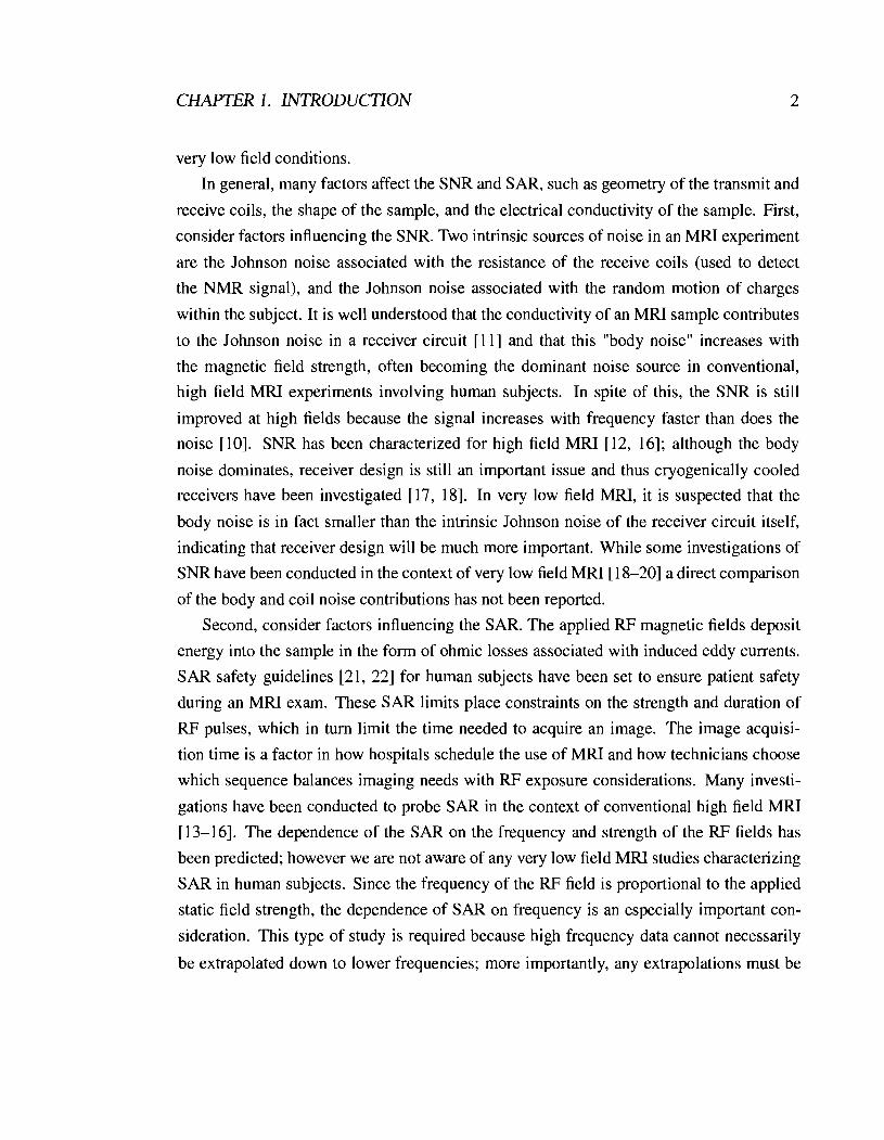
In general, many factors affect the SNR and SAR, such as geometry of the transmit and
receive coils, the shape of the sample, and the electrical conductivity of the sample. First,
consider factors influencing the SNR. Two intrinsic sources of noise in an MRI experiment
are the Johnson noise associated with the resistance of the receive coils (used to detect
the NMR signal), and the Johnson noise associated with the random motion of charges
within the subject. It is well understood that the conductivity of an MRI sample contributes
to the Johnson noise in a receiver circuit [l 11 and that this "body noise" increases with
the magnetic field strength, often becoming the dominant noise source in conventional,
high field MRI experiments involving human subjects. In spite of this, the SNR is still
improved at high fields because the signal increases with frequency faster than does the
noise [lo]. SNR has been characterized for high field MRI [12, 161; although the body
noise dominates, receiver design is still an important issue and thus cryogenically cooled
receivers have been investigated [17, 181. In very low field MRI, it is suspected that the
body noise is in fact smaller than the intrinsic Johnson noise of the receiver circuit itself,
indicating that receiver design will be much more important. While some investigations of
SNR have been conducted in the context of very low field MRI [18-201 a direct comparison
of the body and coil noise contributions has not been reported.
Second, consider factors influencing the SAR. The applied RF magnetic fields deposit
energy into the sample in the form of ohmic losses associated with induced eddy currents.
SAR safety guidelines [21, 221 for human subjects have been set to ensure patient safety
during an MRI exam. These SAR limits place constraints on the strength and duration of
RF pulses, which in turn limit the time needed to acquire an image. The image acquisi-
tion time is a factor in how hospitals schedule the use of MRI and how technicians choose
which sequence balances imaging needs with RF exposure considerations. Many investi-
gations have been conducted to probe SAR in the context of conventional high field MRI
[13-161. The dependence of the SAR on the frequency and strength of the RF fields has
been predicted; however we are not aware of any very low field MRI studies characterizing
SAR in human subjects. Since the frequency of the RF field is proportional to the applied
static field strength, the dependence of SAR on frequency is an especially important con-
sideration. This type of study is required because high frequency data cannot necessarily
be extrapolated down to lower frequencies; more importantly, any extrapolations must be

CHAPTER I . INTRODUCTION 3
verified with definitive experimental data in order to satisfy national health safety criteria.
The purpose of this thesis is to fill the gap in information about SNR and SAR as it
pertains to very low field MRI. I first investigate a model problem consisting of an elec-
trically conducting sphere placed in a uniform oscillating magnetic field. This is followed
by a parallel experiment involving human subjects, allowing realistic conclusions regarding
SNR and SAR for in vivo MRI under very low field conditions to be drawn.
I begin with a classic problem in electrodynamics that involves solving the eddy current
distribution in a conducting sphere placed in a uniform oscillating magnetic field. This
model problem was first explored in the context of MRI by Hoult and Lauterbur [ l 11 and
there exists a large body of MRI literature on this subject [23-251. The primary value of
the problem is that it can be solved analytically - allowing the current density, magnetic
field, and power dissipated by ohmic losses to be written in closed form - and represents
a well-understood reference against which experiments may be quantitatively compared.
I present a method of solution to the problem and give a complete set of expressions for
the current density, magnetic field, and power dissipation in the low field limit. The ohmic
losses and magnetic field were then measured in two independent experiments that involved
exposing spherical phantoms to a weak magnetic field oscillating at frequencies in the range
0.1 to 1.25 MHz. The ohmic losses were measured by detecting the perturbing effect of
the phantom on a resonant circuit, in a technique analogous to cavity perturbation [26].
The oscillating magnetic field in the vicinity of the sphere was measured directly using a
small probe coil. The results from both experiments are seen to be in excellent agreement
with predictions of the model. Previous investigations of this problem have all been at
high frequencies; to our knowledge this experiment is the first full characterization of this
electrodynamic problem in the low frequency limit.
With an understanding of the model problem in hand, similar experiments involving hu-
man subjects were then performed, and yield results that allow conclusions regarding SNR
and SAR of low field MRI experiments to be drawn. These experiments involved exposing
human subjects to low level oscillating magnetic fields produced by nearby coils, similar to
a design used previously as receiver coils for very low field MRI [3, 41. The ohmic losses
in the subject are measured in the same manner as that used for the phantoms, and can be
directly related to the noise that the subject would produce in an MRI experiment. In the
same way, the noise that would be produced by the receive coils was also effectively mea-
CHAPTER I . INTRODUCTION 4
sured. Comparison of these contributions indicates which of the two is the dominant source
of noise under the conditions of the experiment, and the degree to which improvements can
be made by reducing the receiver coil resistance.
The experiment probing SAR was similar to that for SNR, except that a transmit coil
was used in place of the receive coils. Since the field generated by the transmit coil is very
uniform, the power deposition is also relatively uniform within the subject; measurements
of ohmic losses thus reflect the average SAR of energy deposited over the volume of the
subject exposed to the field.
To our knowledge the experiments presented in this thesis are the first that directly
investigate SAR and SNR in human subjects at the frequencies relevant to very low field
MRI.
1 . Outline of thesis
This thesis is structured as follows. In Chapter 2, I present the basics of NMR and MRI, and
introduce MRI of hyperpolarized noble gases in both the low and high field limits; I then
describe the dependence of SNR and SAR on frequency and the role played by the con-
ductivity of the sample, leading to a detailed motivation for this thesis. Chapter 3 contains
a description of the mathematics underlying the problem of a conducting sphere exposed
to a uniform oscillating magnetic field. In Chapter 4, I describe the experimental appara-
tus including the transmit and receive coils; in Chapter 5 I describe the methods used to
collect and analyze the data. Data obtained from experiments on the spherical phantoms
are presented and discussed in Chapter 6, while the same is done for the experiments in-
volving human subjects in Chapter 7. I present the conclusions from this work and make
suggestions for further avenues of research in Chapter 8.

Chapter 2
Background
In this chapter I present background information necessary to put the work described later
in this thesis into context. I begin with a brief classical description of nuclear magnetic
resonance (NMR) and magnetic resonance imaging (MRI) in order to present key concepts.
I then introduce aspects of emerging MRI modalities involving hyperpolarized gases and
very low field strengths. This material is followed by discussions of signal-to-noise ratio
(SNR) and specific absorption rates (SAR) for MRI involving electrically conducting me-
dia, which are essential concepts in this thesis. Finally a detailed motivation for the work
presented in this thesis is given.
2.1 Nuclear magnetic resonance
Nuclear magnetic resonance was discovered independently by Bloch and Purcell in 1946
[27, 281. In a static magnetic field Bo, a spin-112 nucleus tends to align with its magnetic
moment parallel or antiparallel to the magnetic field. Since the parallel state has a lower
energy than the antiparallel state, more nuclei occupy this favoured state at thermal equilib-
rium. A macroscopic sample has a net nuclear magnetization per unit volume M parallel
to the applied field. Denoting the number of parallel and antiparallel nuclei per unit volume
as N f and N - respectively, we define the fractional polarization as

CHAPTER 2. BACKGROUND
The magnitude of the magnetization per unit volume is defined as
where pn is the magnetic moment of a single nucleus and N = NS + N- is the total
number of nuclei per unit volume. The population of nuclei in the parallel and antiparallel
states is described by a Boltzmann distribution. The resulting magnetization is [29]
M = pnN tanh (s) ,
where kg is the Boltzmann constant and T is the temperature. For hydrogen nuclei at body
temperature and experimentally accessible magnetic fields, the argument of Eq. 2.3 is very
small; typically the ratio pnBO/kBT 1 - 10 ppm. As a result, since tanh(x) = x
for small x, the magnetization is proportional to the magnetic field under experimental
conditions:
In a classical sense, the motion of M is described by
where y is the gyromagnetic ratio of the nucleus. If M is aligned at an angle to Bo, Eq. 2.5
describes a precession of M about Bo with an angular frequency
where Bo is the magnitude of Bo and w is the Larmor frequency.' In the reference frame
rotating about Bo at this frequency, M is stationary and there is effectively no magnetic
field.
Consider now the application of a magnetic field B1 (magnitude Bl), rotating about
Bo at the Larmor frequency. In the rotating frame, B1 is stationary and M now precesses
about B1 at an angular frequency wl = yB1. For a B1 applied perpendicular to Bo, M
'Since the field strength and frequency are directly related in this way, field and frequency are often used
interchangeably in the NMR literature.

CHAPTER 2. BACKGROUND 7
is tipped away from Bo in the plane perpendicular to B1. After B1 has been applied for a
period of time t , the angle a between Bo and M is given by
In practice, a linearly oscillating field may be used in place of the rotating field described
above since it can always be broken down into two counter-rotating field components. Com-
monly the Larmor frequency is in the radiofrequency (RF) range and therefore the B, field
is referred to as the RF field or RF radiation; the RF field is often applied in short pulses.
Note also that RF fields that are not applied at the Larmor frequency tend to average to
zero in the rotating frame and do not affect the magnetization except under specialized
circumstances.
After the application of an RF pulse, relaxation processes associated with energy trans-
fer mechanisms cause the magnetization to return to equilibrium. This behaviour is phe-
nomenologically described by the Bloch Equation:
where Bo is applied in the z-direction2, e x , e,, and e , are the Cartesian unit vectors, and
M,, My and M, are the Cartesian components of the magnetization vector M. The constant
Tl is the spin-lattice relaxation time, which represents the time required for M, to return to
its equilibrium value Mo. The constant T2, is the spin-spin relaxation time which represents
the time required for the transverse components M, and My to vanish. The Bloch Equation
has the following general solution:
Mx( t ) = [Mx (0) cos(wot) + My (0) s i n ( ~ ~ t ) ] e - " ~ ~ (2.9)
My ( t ) = [- M,(O) sin(wot) + My (0) c o s ( ~ ~ t ) ] e - ~ ~ ~ ~ (2.10)
Mz ( t ) = Mo + [Mz(0) - ~ ~ ] e - ~ ~ ~ ~ . (2.1 1)
To describe how the resonance is detected experimentally, we first define the transverse
2 ~ h i s choice of coordinate system is the normal convention in NMR. However it will only be used in this
chapter; following chapters use a slightly different coordinate system in which the z-axis is aligned with B1.
CHAPTER 2. BACKGROUND
magnetization as
The resonance can be detected with a nearby coil oriented with its axis perpendicular to
Bo. At the position of the receive coil, the field component parallel to the coil axis varies
sinusoidally as a function of time and is proportional to the transverse magnetization MT(t )
The magnetic flux passing through the coil is proportional to BT and the voltage v in-
duced across the coil - also called an electromotive force (EMF) - is given by Faraday's
Law d@
v ( t ) M - O: wo cos(w0t + 6 ) MT ( t ) + sin(wot + 8) ~ M T ( t ) d t d t
Since the relaxation time T2 is usually much longer than the period of precessional rotation,
we can neglect the second term and write
This equation describes the observed voltage, called a free induction decay (FID). It is
also worth noting that since the field of a magnetic dipole drops off as the third power of
distance, the coil is most sensitive to nearby spins.
The time constants TI and T2 give information about relaxation mechanisms in a mate-
rial, making NMR a useful technique in materials science. Additionally, the local environ-
ment around each nucleus influences its Larmor frequency, making NMR spectroscopy an
invaluable technique for chemists to determine molecular structures. Since the amplitude
of the FID is proportional to the density of the material, NMR is also well suited to bio-
logical samples where the prevalence of water provides a high density of hydrogen nuclei
(protons) for NMR. For more detailed information regarding NMR, the reader is directed
to references [30, 3 1 1.
CHAPTER 2. BACKGROUND
2.2 Magnetic resonance imaging
In the 1970's, Lauterbur and Mansfield independently recognized that NMR could be used
to non-invasively image materials and biological samples [32, 331. This imaging modality
is called magnetic resonance imaging (MRI). I give a brief simplified description of a com-
mon way to acquire images of 'slices' of the sample (tomographic imaging); more detailed
descriptions may be found elsewhere [34, 351.
In tomographic imaging, a 'slice' of the sample to be imaged is selected. A gradient in
the static field Bo is applied across the sample in a direction perpendicular to the desired
slice. In a thin slice of sample where the Larmor frequency matches the frequency of the
applied RF field B1, the nuclear magnetization is tipped away from the axis of the static
field. Application of gradients in Bo causes the Larmor frequency and precession angle (or
phase) of the nuclei within the slice to depend on their position in a precisely defined way.
The voltage induced across the receive coil is a superposition of signals having a form
similar to Eq. 2.17 (the exact form will depend on the way the image was acquired) with
a range of frequencies wo and phase angles 8. The resulting data set can be analyzed with
Fourier transform methods to convert frequency and phase information to a map indicative
of physical properties, such as nuclear density, relaxation rates, and diffusivity.
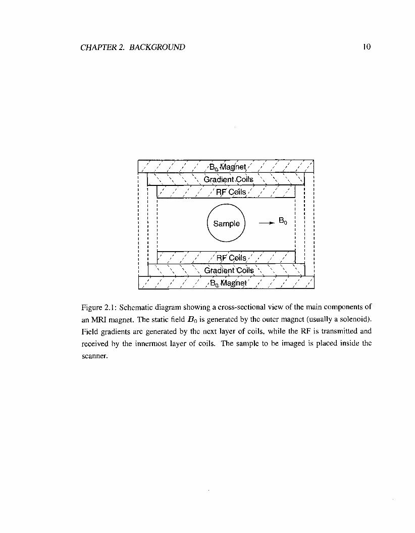
A diagram of the main components of a MRI magnet system are shown in Fig. 2.1. The
static field Bo is usually parallel to the axis of the scanner, in which case it is generated
by a solenoid (shown in the figure as the outermost layer of the scanner). The RF coils are
used to manipulate the precession of the nuclear spins as well as to detect their response
to applied fields. In some experiments, two separate coil systems are used to generate the
RF fields and to detect the NMR signal, while in other cases both functions are served by
a single coil system. Since these coils function as antennas that transmit and receive RF
radiation, they are often referred to as transmit (T,) and receive (R,) respectively. The
T, and R, coils are designed to generate and detect fields in the transverse plane. When
separate T, and R, coils are used, they are usually arranged to be sensitive to perpendicular
components of the transverse magnetization so as to avoid cross-talk, i.e. detection of the
tipping pulses in the R, coils.
Figure 2.2 is a diagram illustrating the functions of the transmit and receive coils. The
transmit coil, shown in the top diagram, provides the RF pulses that are required to ma-
CHAPTER 2. BACKGROUND
. . , I I I I I I I I I I I I
Sample -60 ; ;
Figure 2.1 : Schematic diagram showing a cross-sectional view of the main components of
an MRI magnet. The static field Bo is generated by the outer magnet (usually a solenoid).
Field gradients are generated by the next layer of coils, while the RF is transmitted and
received by the innermost layer of coils. The sample to be imaged is placed inside the
scanner.

CHAPTER 2. BACKGROUND
RF Pulse
FID
Figure 2.2: Block diagram indicating the coupling between the RF coils and the sample.
RF fields are transmitted by the T, coil (top) and received by the R, coil (bottom). The
NMR signal is recorded by a computer. The effective resistance of the R, coil includes
contributions from the sample as well as the coil itself.
nipulate the spins. An unavoidable consequence of the application of RF fields is that they
also generate eddy currents in the sample if it is electrically conducting. The receive coil,
shown in the bottom diagram, detects the FID. The receive coils are primarily sensitive to
two signals: coherent precession of the nuclei (shown by the arrow) and random motions
of charges within the sample (shown by the random path of an electron). I will elaborate on
these statements in following sections.
2.3 MRI of hyperpolarized noble gases
In MRI, the Larmor frequency is selected to excite the nuclei of interest, typically hydrogen
nuclei (i .e. protons) in the water molecules of the sample. Conventional, high field MRI is

CHAPTER 2. BACKGROUND 12
now a successful, well-established technique for detailed imaging of most of the anatomy.
However it is difficult to image cavities such as the lungs where the density of hydrogen
atoms is very low. Lung imaging is further complicated by differences in magnetic sus-
ceptibility between air and tissues which can give rise to strong, inherent field gradients
that accelerate relaxation and impair resolution of images. While specialized techniques do
exist to image lung tissue [36-381, emerging new modalities take a different approach by
imaging pre-polarized noble gases which are inhaled into the lungs. By using laser optical
pumping (OP) techniques [39-41], it is possible to polarize the nuclei of the spin-112 noble
gases 3He and 12'Xe to very high, non-equilibrium levels. This high degree of polariza-
tion is called hyperpolarization (HP) and such gases are referred to as hyperpolarized gases
(HPG). The fractional polarization obtained with OP techniques is approximately 1 O5 times
larger than the polarization obtained in conventional proton imaging, and compensates for
the lower density of the gas (approximately 3000 times less dense than protons in the body)
which would normally make it unviable for MRI. In addition to basic structural informa-
tion, images of HP 3He can also give information about the function and ventilation of the
lungs. For example, 12'Xe actually dissolves into blood and tissue, making it a candidate
to study perfusion and oxygenation. Recommended reviews of HPG MRI include [ 4 2 4 ] .
The first HPG MRI in a biological setting was obtained in 1994 by introducing polarized
I2'Xe into the excised lungs and heart of a mouse [45]. The first in vivo HPG images were
of rat and guinea pig lungs in 1995 [46] and 1996 [47]. Today a number of research groups
routinely acquire in vivo HPG images at high fields for research purposes [43].
Because the magnetization of hyperpolarized gases depends on OP processes rather than
the static field strength, HPG imaging in low magnetic fields should be possible. Because
it is possible, and scientifically relevant, low field HPG MRI is currently being pursued
by a number of groups. The hyperpolarization of gases eliminates the need for the large,
expensive superconducting magnets used in conventional high field imaging. This allows
many new configurations and designs for low field scanners including open geometries,
which are less costly to make and operate [5].
Low field imaging also presents other advantages. Low field scanners are lighter and
therefore more mobile, allowing the orientation of the magnet to be adjusted for imaging a
patient in supine or standing positions 151. Dedicated low field scanners would reduce de-
mands on conventional MRI scanners in hospitals. New possibilities also arise in detection
CHAP7ER 2. BACKGROUND 13
methods; devices such as SQUIDS and other novel receive coils are being explored [6-91. Additionally, gradients caused by susceptibility differences between materials are reduced
in lower fields. An important advantage, and one that is directly relevant to this thesis, is
that the reduced Larmor frequency associated with low frequency operation is expected to
result in a corresponding reduction of the specific absorption rate (SAR) of electromagnetic
energy deposited into the patient [ l 11, making the technique more safe for subjects and
raising possibilities for rapid new RF pulse sequences. This issue is addressed in Sec. 2.5.
Until recently, adaptations of pre-existing conventional high-field MRI technology have
been used exclusively in HPG studies. Low field HPG imaging has been demonstrated in
specialized custom built apparatus. The first published in vivo low field images of HPG in
human lungs below 100 mT were acquired by Venkatesh et al. [2] at a static field strength
of 15 mT, Bidinosti et al. [4] at 3 mT, and Mair et al. [5] at 3.8 mT. The images obtained
by Bidinosti et al. currently represent the state-of-the-art in low field HPG MRI. Currently,
five research groups are actively pursuing low field MRI. These groups are based at S N ,
Carlton University and the Robarts Institute, the Ecole Normale Supirieure (LKBIOrsay),
Haward University (Haward-Smithsonian and Brigham Women's Hospital), and the Uni-
versity of California at Berkeley. Since low field HPG MRI is a technique in its infancy,
many of the issues that are well characterized at high fields have not been studied in detail
at low fields. The quality of low field images lags behind that of high field images of HP
gases; however it is believed that this situation is largely a result of the use of technology
that has not been optimized for this type of imaging, rather than a fundamental limitation
on the SNR. To clarify why this is the case, I now discuss some of the factors influencing
the intrinsic SNR of an MRI image.
SNR Considerations in MRI
The image quality in MRI experiments is clearly linked to SNR. While the average SNR
of an image ultimately depends on many factors, here we only consider the intrinsic SNR
limited by fundamental factors. These factors were recognized when MRI was originally
developed [lo, 1 1 1. The intrinsic SNR is the ratio of the detected signal amplitude to the intrinsic noise
level. The signal is the amplitude of the FID induced in the receiver coil and the intrinsic

CHAPTER 2. BACKGROUND 14
noise is the thermal noise associated with random motion of charges in the receiver coil
and sample. As described in Section 2.1, the FID amplitude is proportional to both the
magnetization and the Larmor frequency:
where we are now using the frequency f = wo/(2.rr) and it is implied from now on that
frequencies refer to Larmor frequencies.
The frequency dependence of the magnetization is very different in the cases of conven-
tional and HPG imaging. In conventional imaging, the nuclear magnetization is established
by the static magnetic field Bo . As described in Section 2.1, the equilibrium magnetization
is proportional to the nuclear density N and static field strength Bo, which in turn deter-
mines the Larmor frequency (Eq. 2.6); thus we obtain the dependence of the conventional,
equilibrium magnetization on the frequency:
Since it is not possible to change the temperature of the subject, increasing the Larmor fre-
quency is the only way to increase the magnetization in conventional imaging. In contrast,
HP gases are magnetized outside the body to very high non-equilibrium levels. The effect of
the static field Bo on the magnetization is negligible in comparison, and the magnetization
of an HPG is given by
MHPG = pnPN (2.20)
where P depends on the details of the OP processes used to generate it, rather than Bo.
Returning to the thermal noise, its behaviour can be understood if we now consider the
RF detection circuit. If the sample is conducting, random motions of charges in the sample
induce corresponding voltages in the receiver circuit. This type of noise in a circuit is well
understood through the fluctuation-dissipation theorem and is called Johnson noise. The
Johnson noise of a resistor R has a root mean-square voltage amplitude of
where Af is the receiver bandwidth. Because the conductivity of the sample results in
Johnson noise in the receiver, the effect of the sample may be modeled as an additional

CHAPTER 2. BACKGROUND
Figure 2.3: Cross-sectional view of the receiver coil wire. In the limit where the skin depth
is much smaller than the wire radius, the conducting area is approximated by a narrow layer
(of width 6) at the surface of the wire.
resistance in the receiver circuit. This additional resistance is called the effective sample
resistance and denoted R,.
Combining the fact that the total effective resistance in the receive coil is the sum of
the resistance of the receive coil itself (Rcoil) and the effective sample resistance R, with
Eqs. 2.18 and 2.21, we obtain
SNR rn Mf (2.22) d z x z '
The resistances Rcoil and Rs have frequency dependencies that can be understood by con-
sidering the good conductor and weak conductor limits. The resistances depend on the
relative sizes of the sample or the wires in the coil compared to the skin depth:
for a material with bulk conductivity a and permeability p. When the radius b of the wire
making up the coil is thick compared to 6, (the "thick limit") the conducting cross-sectional
area may be approximated as a circle of thickness 6 at the outer edge of the wire as shown
Fig. 2.3. The resistance per unit length of the wire is then given by

CHAPTER 2. BACKGROUND
Very Low Field: Low Field j High Fie19 ' I
I I I I 0 I I I 0 I I 0 I I I I
I I 1 I I I
0 I I
/-lorn$ -100mT j - I T 0 I I I
I 0 I I I
Frequency
Figure 2.4: Frequency dependence of the resistance of the body or sample (dashed curve)
and receive coil (solid curve) on a log-log plot. The sample resistance has an f behaviour
and the coil resistance has an f ' I 2 behaviour. The high field regime encompasses conven-
tional MRI techniques. The crossover (low field) and very low field regimes are currently
being investigated.
The behaviour of the resistance in the opposite limit when the sample is thin compared
to the skin depth ("thin limit") has been considered by Landau and Lifshitz [48] (in the
case of a wire), who show that the resistance presented to inductively driven currents is
proportional to f 2. In Chapter 3 this result will be shown in detail for a conducting sphere.
The idealized frequency dependencies of Rcoil and R, are thus
as shown in Fig. 2.4. In practical high field situations (- 1.5 T), the body noise usually
dominates over the coil noise. The term 'low field' generally refers to the crossover region,
where the two resistances are comparable, (roughly in the range 0.1 to 1 T) and the term
'very low field' usually refers to the studies conducted in the range 1 to 100mT. 'Ultra

CHAPTER 2. BACKGROUND
low field' designates the region being explored by SQUID-detected techniques at pT fields.
Now we may summarize the frequency dependence of the SNR in both conventional and
HPG imaging. We define two limiting cases, the body-dominated regime and the coil-
dominated regime, indicating which source of Johnson noise is most prevalent. Combining
Eqs. 2.22 and 2.25, the SNR under coil-dominated conditions is given by
Body-dominated
Coil-dominated
while under body-dominated conditions, Eqs. 2.26 and 2.22 give
Making use of Eqs. 2.19 and 2.20 we may write the frequency dependence of the intrinsic
SNR for both conventional and HPG imaging, as summarized in Tab. 2.1. The relative
sizes of Rs and Rcoil determine the operating regime (and hence frequency dependence),
while their absolute sizes influence the overall magnitude of the SNR. Clearly the SNR
in conventional imaging benefits from an increased Larmor frequency; however in HPG
imaging, the SNR increases only until the crossover to the body-dominated regime has
been made, above which improvements are negligible.
The crossover between the coil-dominated and the body-dominated regimes may be a
favourable operating point for imaging. Many calculations, simulations and measurements
have been carried out to characterize SNR [lo-12, 16, 491 at high fields but only a few
investigations have probed SNR at low frequencies [18-201.
One way in which SNR might be improved can be understood by considering Fig. 2.4.
The body resistance cannot be changed, but at low fields the resistance of the coil may
Table 2.1 : Dependence of the intrinsic SNR on frequency in the coil-dominated and body-
dominated noise regimes, for both conventional and HPG MRI.
Intrinsic SNR
Conventional
m f K f 7/4
HPG
constant f 3/4

CHAPTER 2. BACKGROUND
Frequency
Figure 2.5: Frequency dependence of the resistance of various RF receivers for MRI, as it
would appear on a log-log plot. As in Fig. 2.4, the resistance of the body (dashed curve) and
receive coil (solid curve) are shown for comparison. Additionally the potential behaviour of
cooled resistive coils, superconducting coils, and SQUID sensors are shown. The frequency
at which the crossover between the body resistance dominated regime and coil resistance
dominated regime occurs is reduced when alternative designs are used.
become the dominant noise source. Gains may be made to the SNR by redesigning the
receive coil to have a lower resistance. This might be done by cryogenically cooling the
windings and/or using superconducting or Litz wire. Alternatively, novel new sensors based
on SQUIDs are being investigated.
In fact, combinations of these ideas have been used in numerous studies; for example
cold normal conductors have been used at high frequency [17], superconducting coils are
available commercially and have been used at low fields [50], and the use of superconduct-
ing coils coupled to SQUIDs have been demonstrated [5 11. Litz wire has been used in both
transmit coils [52, 531 and receive coils [54]. A detailed discussion of cryogenic RF coils
is given in [I 81.
The idealized frequency dependence of the effective resistance of cooled resistive coils,
superconducting coils, and SQUID detectors have been sketched in Fig. 2.5 along with that

CHAPTER 2. BACKGROUND
1 Tissue I Low frequency o (Slm)
Muscle 0.07 (perpendicular to fibres) 1 I 0.86 (parallel to fibres)
I Bone ( 0.04 I I Blood 1 0.60 I
Table 2.2: Electrical conductivities of various tissues [I 31.
of resistive room-temperature coils, and the sample (or body) resistance. Comparison of
these curves indicates the potential gains to SNR that might be made through appropriate
coil design. The crossover between the body resistance-dominated and coil resistance-
dominated regimes is expected to occur at lower fields if designs other than conventional
room temperature resistive coil designs are used.
2.5 SAR Considerations in MRI
We now turn to the question of the SAR in conducting samples. The RF and other time-
varying applied fields used in MRI drive eddy currents in the sample, resulting in the dissi-
pation of energy. The weak electrical conductivity of the body is the dominant mechanism
for the absorption of electromagnetic energy in human subjects. Measured values of vari-
ous tissue conductivities have been reported [13, 551, and most tissues are seen to have a
conductivity less than 1 S/m (Tab. 2.2).
The SAR is defined as the time-averaged rate of energy absorption per kilogram of
sample - i.e. power per kilogram,
< P > SAR = -
where P now represents the total average power and m, is the mass of the sample. It will be
shown in Chapter 3 that the power absorbed from B1 is

CHAPTER 2. BACKGROUND
I Site I Dose Time (min) I SAR I
/ head 1 averaged over I 10 1 3
whole body
Table 2.3: SAR guidelines for magnetic resonance diagnostic devices, according to the US
Food and Drug Administration [2 1 1.
averaged over
head or torso
extremities
In the thin limit, R, is proportional to f by Eq. 2.26, which we combine with Eqs. 2.29
and 2.30 to give
SARcx B ? R , ~ B ? f 2 . (2.3 1)
For a given operating frequency, SAR safety guidelines effectively place constraints on the
strength and duration of the RF pulses. This in turn limits the speed at which an image
can be acquired. In conventional imaging, 180" tipping pulses (also called T-pulses) may
be as short as a few milliseconds. In very low field applications, it should be possible to
increase the strength of B1 to rotate nuclei through the same tip angle on a much shorter
timescale while keeping the same SAR. A summary of SAR recommendations for magnetic
resonance imaging as given by the United States Food and Drug Administration [21] is
presented in Tab. 2.3. These values indicate levels that put the patient at significant risk.
Recommendations made by Health Canada [22] are less explicit, but consistent with those
of the USFDA. SAR in MRI has been extensively investigated at high frequencies [13-161.
equal to or greater than:
15
per gram of tissue
per gram of tissue
2.6 Experimental motivation
(Wkg)
4
The motivation behind this thesis is twofold. First, since the SNR of an MRI image depends
on the sizes of R, and RCoil, choices of coil design and operating frequencies rely heavily on
an understanding of their behaviour. This thesis presents a measurement of R, for human
subjects, characterizing the dependence on frequency and sample size. These results will
help in the design of receive coils as well as optimization of the operating frequency for
very low field MRI.
5
5
8
12

CHAPTER 2. BACKGROUND 2 1
Second, the SAR of human subjects during an MRI exam directly affects the RF pulse
sequence design. An understanding of R, is thus fundamental to characterization of the
SAR in conducting samples. The frequency dependence of Rs as it pertains to SAR is also
examined as part of the investigations presented in later chapters of this thesis. In both cases
(ie. SNR and SAR), this work is believed to be the first of its kind in the context of very
low field MRI.
Before experiments on human subjects can be done, we must first understand a model
problem and demonstrate that we can successfully measure R, of a model system, or phan-
tom. This work presents a complete investigation of the model problem of a spherical con-
ducting sample placed in a uniform oscillating magnetic field, focusing on the frequency
range 0.1 - 1.25 MHz. First, I present a mathematical analysis of the analytic solution to
this problem, which gives predictions for the current density, magnetic field, and power
dissipation, (which in turn is related to R,). Next, measurements of the sample resistance
R, and magnetic field perturbation of spherical phantoms are presented and compared to
the prediction of the model. These measurements were performed by exposing samples
to a weak uniform oscillating magnetic field produced by a very low field MRI transmit
coil. The coil constitutes the inductive element in a tuned resonant circuit, and the sample
perturbs the quality factor and magnetic field map of the circuit due to the induced eddy
currents. The induced losses in the sample are modeled as an additional resistance R, in
the resonant circuit, determined from measuring the change in the quality factor when the
sample enters the vicinity of the circuit. The oscillating magnetic field in the vicinity of a
spherical phantom was also measured in several locations using a small probe coil. Both
the results of R, and magnetic field measurements are compared to the model.
With a complete understanding of the model problem in hand, measurements of R, for
human subjects become meaningful. Measurements of the effective sample resistance R,
of human subjects are presented in two variations. The experimental setup is exactly the
same as that used for measuring R, in spherical samples; that is, by detecting the perturbing
effect of a sample on a resonant circuit.
To investigate SNR, we used receive coils as the inductive element. These coils were
designed to mimic those used in a very low field MRI experiment [3, 41. These coils
are useful because they couple closely to the body and thus have a high sensitivity. This
experiment gives practical values of the resistances Rs and RWil over the frequency range

CHAPTER 2. BACKGROUND 22
0.01 - 1.25 MHz. The absolute size and the relative frequency dependence of each term is
indicative of the SNR encountered in very low field MRI experiments.
To investigate SAR, the same experiment was repeated using a uniform B1 coil (i.e. a
transmit coil) rather than the receive coils, to measure R, over the frequency range 0.1 -
1.25 MHz. Since the field is uniform, the value of R, that we measure is much more in-
dicative of the overall average SAR that is encountered in low field MRI of human subjects.

Chapter 3
Spherical model
In this chapter, I present a mathematical analysis of the problem of a conducting sphere
placed in a uniform oscillating magnetic field. Determination of the eddy current distribu-
tion in the sphere and the resulting field profile give predictions which may be compared to
experiments.
The sphere is often used as an example in textbook problems in electromagnetism be-
cause it is a geometrically simple object, leading to tractable solutions. Investigation of
an analytically convenient problem provides a foundation upon which to study more com-
plicated systems. The problem of finding the eddy current distribution and magnetic field
when a uniform conducting sphere is placed in a uniform oscillating magnetic field is rel-
evant to a wide range of applications. A correspondingly wide range of approaches have
been taken to find solutions to the problem. It is addressed in general electromagnetism
textbooks [56, 571 but also appears in the literature of specific disciplines where the prob-
lem is relevant. Analytical expressions for eddy-current distributions in conducting media
are of interest to engineers and geophysicists; inducing eddy currents in a material allows
non-destructive testing for defects [%I, and eddy-current probes can give information about
the materials inside geological bore holes [59]. Among other applications, understanding
the role played by eddy currents in determining the performance and efficiency of motors
constitutes a sizeable field in engineering [60]. Further discussions of eddy-current losses
in spheres from these viewpoints can be found in References [6 1-65].
Hoult and Lauterbur were the first to investigate eddy-current losses in conducting sam-
ples [I I] from the viewpoint of MRI. Their 1979 paper in which intrinsic SNR limitations

CHAPTER 3. SPHERZCAL MODEL 24
were recognized and estimated represents a landmark in the development of modem MRI.
They considered both the dielectric losses associated with the distributed capacitance of
the RF coils, and the inductive (or magnetic) losses associated with induced eddy currents.
While it is possible to reduce dielectric losses through coil design and specialized shields,
the inductive losses are fundamental and constitute the focus of this thesis.
Hoult and Lauterbur calculated the rate at which energy is absorbed by a homogeneous,
conducting sphere (conductivity a, permittivity E , permeability p) in a uniform RF magnetic
field (amplitude B1, angular frequency w ) in the limit when the wavelength of the RF field
inside the material is much larger than the sample. Another assumption in the analysis is
that the skin depth of the RF field inside the sphere is so large compared to the size of the
sample that its effect can be neglected completely. This second assumption makes their
analysis extremely simple in comparison to most of the references cited above.
More advanced analyses of the sphere problem in the context of MRI include effects
of the skin depth in the limit when it is larger than the sample but cannot necessarily be
neglected (the thin limit). Carlson [66] solved the problem for the non-magnetic sphere
(p = pg, the permeability of free space) in the thin limit to obtain more complete expres-
sions of the current density and magnetic field. It is worth noting that despite the widely
recognized importance of Hoult and Lauterbur's results (their paper has been cited some
400 times to date) and the numerous related articles in the MRI literature [23-251, many of
the results published after Hoult and Lauterbur's work contain errors. Particularly lacking
are consistent, explicit expressions for the absorbed power and magnetic field. In this chap-
ter 1 provide a summary of the correct versions of some results of this solution, under the
conditions relevant to MRI. Complete results including some additional ones we have not
found in existing literature are being prepared for publication [67].
Method of solution
Figure 3.1 illustrates the problem at hand: a uniform conducting sphere of radius a is placed
in an applied, uniform oscillating magnetic field B1 = BlePiwte,. We use spherical co-
ordinates, where r is the radial position, 4 is the azimuthal angle, 0 is the polar angle, and
e,r, e4 , and ee are the unit vectors in each of these directions, respectively. Electromag-
netism in homogeneous linear media is handled with Maxwell's Equations for the magnetic

CHAPTER 3. SPHERTCAL MODEL
Figure 3.1: Schematic representation of a conducting sphere in a uniform oscillating mag-
netic field. The field is uniformly polarized in the z-direction.
field B and E in such materials, which are
dE V x B = p u J + p ~ -
at
where pf is the free charge density and J is the free current density. The complete problem
is specified by including Ohm's Law
The free charge density pf is essentially zero.'
'Even if there were a net charge on the sphere, it would flow to the surface on a timescale T = €/a. In a
physiological context, a N 1 S/m and em,, N 9 0 ~ which corresponds to T-' N 80 GHz. Our experiments
are performed at frequencies up to .U 1 MHz and thus it is perfectly reasonable to ignore free charge in the
interior of the sphere. Furthermore, the total number of ions introduced into our samples is so large that the
sphere would have to be charged to a very high potential before free charges would influence the ohmic losses.

CHAPTER 3. SPHERICAL MODEL 26
There are many methods for solving Maxwell's equations in the context of this problem.
Jackson [68] and Carlson [66] use an expansion in vector spherical harmonics to determine
B; Harpen [25,69] uses the vector potential. A more direct approach is provided by London
[70], in which the current density J is solved and used to calculate the fields. I will follow
London's discussion; first I will follow the discussion presented by Griffiths [7 11 to derive
the appropriate wave equation.
We begin with substitution of Eq. 3.5 into Eq. 3.3. Taking the curl of the resulting
equation gives a v x (V x J ) = -O- (V at x B). (3.7)
Making use of Eq. 3.4, Eq. 3.6 and the vector identity
we obtain
We look for time harmonic solutions to the current density, reflecting the harmonic nature
of the applied field:
J ( T , t ) = ~ ( r ) e - ' ~ ~ (3.10)
and thus Eq. 3.9 yields the wave equation
where the wavenumber k is defined as
The symmetry of the problem determines the general form of allowed solutions for
the current density. The applied field breaks the symmetry in the polar direction, but the
currents cannot depend on the azimuthal angle 4. The currents must have closed paths as
implied by Eq. 3.1 and the finite nature of the sample. These facts combined with Eq. 3.3
imply that the currents can only flow in the azimuthal direction:
CHAPTER 3. SPHERTCAL MODEL 27
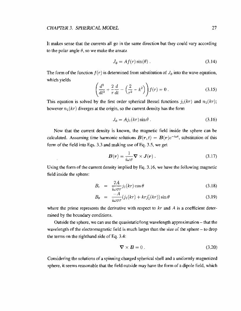
It makes sense that the currents all go in the same direction but they could vary according
to the polar angle 8, so we make the ansatz
J4 = A f ( r ) sin(8) . (3.14)
The form of the function f ( r ) is determined from substitution of J4 into the wave equation,
which yields
This equation is solved by the first order spherical Bessel functions j l(kr) and nl(kr);
however nl(kr) diverges at the origin, so the current density has the form
J4 = A jl (kr) sin 8 . (3.16)
Now that the current density is known, the magnetic field inside the sphere can be
calculated. Assuming time harmonic solutions B ( r , t ) = B(r)ePiwt, substitution of this
form of the field into Eqs. 3.3 and making use of Eq. 3.5, we get
Using the form of the current density implied by Eq. 3.1 6, we have the following magnetic
field inside the sphere:
2A . B, = -jl(kr) cos8
zwor - A
Be = - ( j l (kr) + krji (kr)) sin 8 zwor
where the prime represents the derivative with respect to kr and A is a coefficient deter-
mined by the boundary conditions.
Outside the sphere, we can use the quasistatic/long wavelength approximation - that the
wavelength of the electromagnetic field is much larger than the size of the sphere -to drop
the terms on the righthand side of Eq. 3.4:
Considering the solutions of a spinning charged spherical shell and a uniformly magnetized
sphere, it seems reasonable that the field outside may have the form of a dipole field, which

CHAPTER 3. SPHERICAL MODEL 28
is irrotational. Thus we make the ansatz that the field outside is the combination of the
applied field B1 and an induced dipole field of dipole moment m:
B ( r > a ) = B1+ - ' O m ( 2 cos 0e, + sin Oee 47rr3 )
which may also be written as
To find A and m , we use the boundary conditions on B
Pan B(a)an x n = -B(a)out x n Pout
where n is the unit vector normal to the surface of the sphere. Outside the sphere we
have free space (pout = po); combining the field (Eq. 3.22) with the boundary conditions
(Eq. 3.23) we now have
2 A - j1 ( k a ) cos I9 = ( B ~ + w) cos I9 zwaa 47ra3
-A PO m - ( j l ( k a ) + ka j ; ( k a ) ) sin 0 = ( - B1 + 7) sin 0 iwaa 47ra
which may be simplified by making use of two properties of spherical Bessel functions [72]
resulting in

CHAPTER 3. SPHERICAL MODEL
In the case of a non-magnetic sphere ( p = PO), Eqs. 3.28 and 3.29 reduce to
3iwa A =
2kjo(ka) 27ra3 Bl j2 ( k a )
m = Po jo(ka) '
Now that we have the coefficients A and m, we may write expressions for the radial and
polar components of the magnetic field inside the sphere
and outside the sphere
- B1 sin 0 1 Be =
j o ( W OW) - +(W)
In Cartesian coordinates, the field inside the sphere is
while outside the sphere
3Bl j2 ( k a ) a3xz Bx = --- 2 jo (ka) r5
3B1 j2 ( k a ) a3yz By = --- 2 jo (ka) r5
'It can be seen that the corresponding result published by Carlson [66] must have an error since V . B # 0
(as pointed out by Petropoulos [24]).

CHAPTER 3. SPHERICAL MODEL 30
The current density J dissipates energy in the form of ohmic losses. The time-averaged
power is given by: 1
< P >= - / 1.q2dv . 2a
(3.38)
This integral can be evaluated by recognizing that the spherical Bessel function jv-112(x)
is related to the ordinary Bessel function J,(x) by j,-l12 ( x ) = J ~ J , ( x ) ; this allows
identities involving the Bessel functions to be used. Equation 3.38 can be evaluated and
expressed in many ways, depending on which of the following identities is used:
a la r ~ , ( k r ) ~ , ( l r ) d r = [k JL ( k r ) J,(lr) - 1 JL ( l r ) J,(kr)] 12 - k 2
(3.39)
- a -
k 2 - 12 [ J + ( ) J ) - + I ( 1 ) ( I (3.40)
- a - [k J ( r ) J ( r ) - 1 - 1 ( 1 ) ( I (3.41)
12 - k2
Carlson writes the result as
37rwBT < P > = 1m [k* jl ( k a ) j;' ( k a ) ]
~ l ~ I ~ j o ( k a ) l ~
where I m ( x ) denotes the imaginary part of x and z* denotes the complex conjugate of z .
Petropoulos [24] expresses the power in a similar way but has assumed the opposite sign
for the exponential eiwt; rewriting his result to be consistent with our notation we obtain
37rw B?a2 < P > =
PlkI2jo(ka) l 2 1m [k* j2 ( k a ) jl ( k 'a ) ] .
While Petropoulos states that these results are not the same, in fact it can be shown that
both results are equivalent to
or, in a form that more directly shows the relationship to the current density,

CHAPTER 3. SPHERICAL MODEL
In the low-frequency limit E w << a , the real part of k2 may be neglected, giving
where 6 is the skin depth (Eq. 2.23). Since we are in the thin limit where a 5 6, the Bessel
functions may be expanded about k = 0 to express the power in terms of a/6. The series
expansion of the Bessel functions appearing in the expressions are
Substitution of the first two terms in the expansion given by Eq. 3.50 into Eq. 3.37 allows
the magnetic field outside the sphere to be written in terms of a/6:
while inclusion of the third term allows Eq. 3.45 to be written as

CHAPTER 3. SPHERICAL MODEL 3 2
This expression is equivalent to Eq. (19) in Ref. [66]. The first term is the result obtained
by Hoult and Lauterbur when the skin depth is ignored.
This power is linked to the ohmic losses, modeled by including an effective sample
resistance R, in the circuit responsible for generating the magnetic field. If the peak current
in that circuit is denoted I , then the RMS power dissipated by the effective resistance is:
For a coil that produces a homogeneous field
x = B1/I, the magnet constant of the coil,
readily accessible experimental parameters:
over the sample volume, we may substitute
which allows us to express R, in terms of
Equation 3.58 is the primary expression for the sample resistance against which compar-
isons with experimental data are made in Chapter 6.
3.2 Interpretation
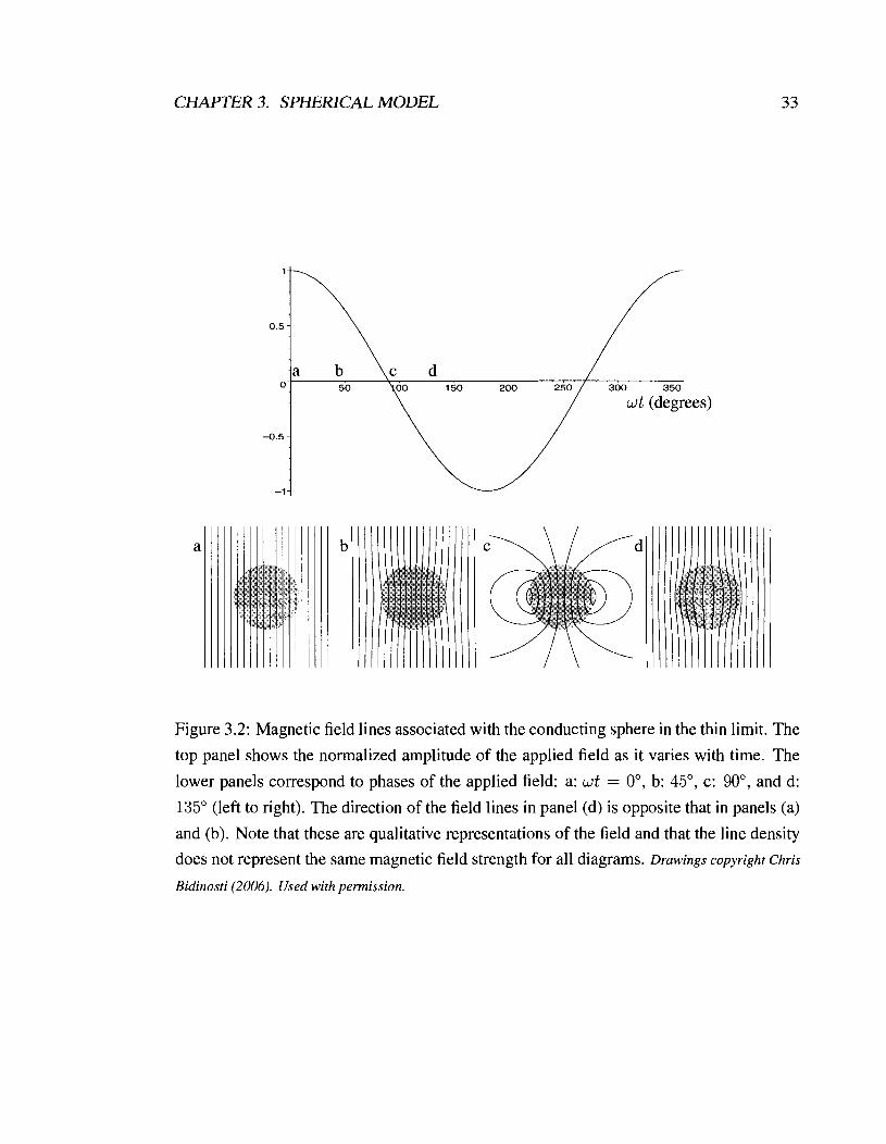
The magnetic field lines associated with the solution for B (Eqs. 3.36,3.37) in the case of a
weakly conducting sphere are shown in Fig. 3.2 as they depend on the phase of the applied
field. The results can be interpreted by keeping in mind that the applied field amplitude is
B1 = B1 cos(wt). When wt = 0•‹, the applied field is at its peak amplitude and the induced
field is close to its minimum strength. As the phase increases, the applied field strength
drops and the induced field strength increases, hence increasing the field line density inside
the sphere. At 90•‹, the applied field vanishes and the induced field is nearly a maximum. As
the phase passes through 135", the applied field is dropping less rapidly; thus the induced
field weakens. However as the applied field has changed sign, the overall field strength
inside the sphere is reduced. When the applied field changes direction at 180•‹, this cycle
repeats with the induced currents now flowing in the opposite sense. In general, we expect
the induced field to be out of phase with the applied field. The phase is an indication of
the impedance of the sphere; if it were perfectly inductive (i.e. lossless), the induced field
would be out of phase with the applied field by 180". If the sphere was purely resistive the
CHAPTER 3. SPHERlCAL MODEL
Figure 3.2: Magnetic field lines associated with the conducting sphere in the thin limit. The
top panel shows the normalized amplitude of the applied field as it varies with time. The
lower panels correspond to phases of the applied field: a: w t = 0•‹, b: 45", c: 90•‹, and d:
135" (left to right). The direction of the field lines in panel (d) is opposite that in panels (a)
and (b). Note that these are qualitative representations of the field and that the line density
does not represent the same magnetic field strength for all diagrams. Drawings copyright Chris
Bidinosti (2006). Used with permission.

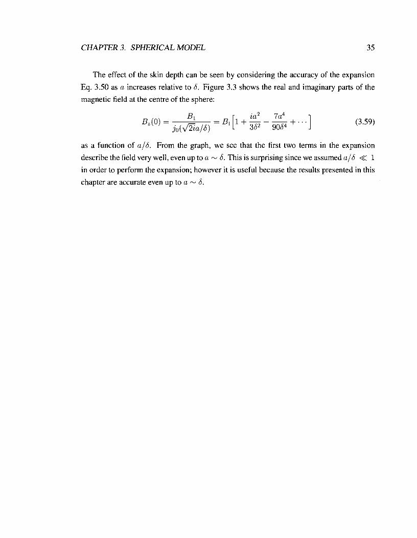
CHAPTER 3. SPHERICAL MODEL
Figure 3.3: Lowest order contributions to the field components at the origin (centre of
sphere). The solid lines represent the exact solution and the dashed lines represent approxi-
mations; the real part includes the applied field and the first real term in the expansion, and
the imaginary part shows the first imaginary term in the expansion. Drawing copyright Chris
Bidinosti (2006). Used with permission.
induced field would be 90" out of phase with the applied field. From the plots of the field
for a weakly conducting sphere shown in Fig. 3.2, the phase lag between the induced and
applied fields is close to 90•‹, showing the sphere is mostly resistive. From the expansions
used in the above analysis, we see that the deviation from a 90" phase lag depends on the
relative size of a and 6.
CHAPTER 3. SPHERICAL MODEL 35
The effect of the skin depth can be seen by considering the accuracy of the expansion
Eq. 3.50 as a increases relative to 6. Figure 3.3 shows the real and imaginary parts of the
magnetic field at the centre of the sphere:
as a function of a/6 . From the graph, we see that the first two terms in the expansion
describe the field very well, even up to a - 6. This is surprising since we assumed a / 6 << 1
in order to perform the expansion; however it is useful because the results presented in this
chapter are accurate even up to a -- 6.

Chapter 4
Apparatus
In this chapter I describe the apparatus that were used in the experiments to measure ohmic
losses and magnetic fields associated with eddy currents in weakly conducting samples.
First, I describe the coils and circuitry that were used to generate and detect oscillating
magnetic fields. Second, I describe the samples that were used and how they were posi-
tioned inside the coil. Last, I describe the instruments and data acquisition.
4.1 Transmit coil
In Chapter 3, I presented the mathematical analysis of a conducting sphere in a uniform
oscillating magnetic field. To do the corresponding experiment, such a magnetic field is a
primary requirement. In this section I describe the coil that was used to generate this field.
4.1.1 Coil design
As mentioned in Sec. 2.2, a cylindrical solenoid is usually employed in MRI to generate the
static magnetic field Bo, aligned with the solenoid axis. The coil producing the B1 field,
called the transmit or B1 coil, has to be designed to fit within the Bo solenoid, generate a
field in any direction perpendicular to Bo, and leave enough room inside for a subject.
It has long been recognized that a cylindrical coil arrangement called a saddle or saddle-
shaped coil pair generates a uniform, transverse magnetic field near its midpoint. One sad-
dle coil consists of two parallel wiresjoined by arcs called the return paths. A saddle coil

CHAPTER 4. APPARATUS
Figure 4.1: Sketch of a saddle coil arrangement. Currents flowing through the long straight
wires (as indicated by arrows) generate an approximately uniform, transverse magnetic field
inside the coil. The direction of the field is defined as the z-direction to be consistent with
the analysis presented in Chapter 3.
pair having the is shown in Fig. 4.1. The highest field homogeneity is achieved when the
parallel wires are located at values of the azimuthal angle 4 of f 60•‹, f 120". By super-
imposing a number of saddle coils subtending various angles, we can increase the field
homogeneity. It is a well known that a wire spacing that is sinusoidal in the azimuthal an-
gle q5 generates a perfectly uniform field (when the cylinder is infinite) [73, 741; hence by
spacing the wires in a sine-phi distribution we obtain a close approximation of a uniform
field inside the coil.
In practical applications, the performance of this type of design is excellent when driven
with a low frequency current, but degrades at higher frequencies as the wavelength ap-
proaches the length of wire in the coil and currents in one region of the coil become out of
phase with currents in other regions.
The field produced by this coil is linearly polarized, since it oscillates between pointing
in the +z-direction and the -2-direction. I mentioned in Sec. 2.1 that a circularly polarized
field can also be used in NMR (although this requires the phase of the currents in each of

CHAPTER 4. APPARATUS
0 infinite coil
0 this design
0.~2 0 0.2 0.4 z-direction 0.6 0.8 1
Figure 4.2: This diagram displays the locations of the wires in the transmit coil. The first
quadrant of a unit cylinder is shown from the end-on view. The circles show the ideal
positions for an infinite cylinder [75]. The diamonds show the positions of the wires as
optimized by computer simulation of this truncated coil.
the parallel wires be set appropriately). For a given NMR tip angle a, the SAR associated
with a circularly polarized field is half that produced by a linearly polarized field.
For the experiments presented in this thesis, we used a sine-phi coil designed specif-
ically to be a B1 transmit coil for very low field MRI [76]. The transmit coil consists of
five saddle coil elements constructed from a single continuous length of 1 mm diameter
solid copper wire wound on a hollow, cylindrical, fibreglass form. The axial length of the
transmit coil is 90 cm and its diameter is 54 cm, suitable dimensions for use in an MRI
scanner designed to accommodate a human torso. The total length of wire is - 30 m and
its self-resonance frequency is - 1.9 MHz. The angular positions of the wires that optimize
the field homogeneity can be predicted exactly for an infinite cylinder [75]; truncation of
the cylinder affects the homogeneity of the resulting field. To compensate for truncation
effects, the field profile of this coil was calculated including contributions from the return
paths. The optimal wire positions were determined using a computer algorithm to maximize
the field homogeneity.

CHAPTER 4. APPARATUS 3 9
Figure 4.2 shows the optimal angular position of wires for one quadrant of this transmit
coil. Also shown are the wire positions from the analysis of the infinite coil. We define the
z-direction to be the direction of the B1 field to be consistent with the analysis presented
in Chapter 3. The axial direction is defined as the y-direction. Note that I have now made a
change from the normal convention used in Chapter 2, in which the static field Bo defined
the z-direction. In all further discussions, the z-direction refers to that of B1.
4.1.2 Coil performance
The transmit coil described above has been characterized extensively. When driven with an
oscillating current at frequencies below its self-resonant frequency it produces an oscillating
field that is homogeneous to within 1.5% over a 12 litre volume: 15 cm in each transverse
direction (x and z) and 10 cm in the axial direction (3) from the centre point of the coil
(called the isocentre). Figure 4.3 shows a comparison of the calculated and measured field
strength inside the transmit coil. The total normalized calculated magnetic field in the xz-
plane is shown in the top left panel of the figure. Clearly the field is very uniform near the
isocentre of the transmit coil. The top right panel in Figure 4.3 shows the z-component
of the magnetic field (the dominant component near the isocentre), in a narrower field of
view highlighting the most homogeneous region of the field in more detail. With human
imaging in mind, the axial homogeneity is of interest considering the aspect ratio of the
volume that will generally be occupied by a subject. The lower left panel in the figure
shows the normalized calculated z-component of the magnetic field in the yz-plane, which
can be directly compared to the lower right panel showing experimental data [76] for the
z-component of the field over a similar range. This comparison shows that the z-component
is homogeneous at the 0.5 % level over a 20 cm x 20 cm area in the centre of the yz-plane.
These data demonstrate that the performance of the transmit coil is consistent with design
specifications.
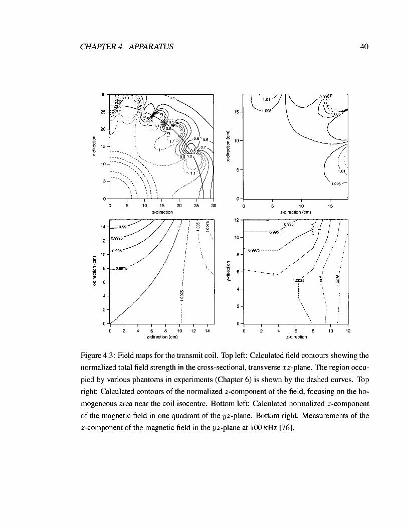
CHAPTER 4. APPARATUS
0 5 10 15 20 25 30 z-direction
0 5 10 15 z-direction (crn)
0 2 4 6 8 1 0 1 2 1 4 z-direction (crn)
0 2 4 6 8 1 0 1 2 z-direction
Figure 4.3: Field maps for the transmit coil. Top left: Calculated field contours showing the
normalized total field strength in the cross-sectional, transverse xz-plane. The region occu-
pied by various phantoms in experiments (Chapter 6) is shown by the dashed curves. Top
right: Calculated contours of the normalized z-component of the field, focusing on the ho-
mogeneous area near the coil isocentre. Bottom left: Calculated normalized z-component
of the magnetic field in one quadrant of the yz-plane. Bottom right: Measurements of the
z-component of the magnetic field in the yz-plane at 100 kHz [76].
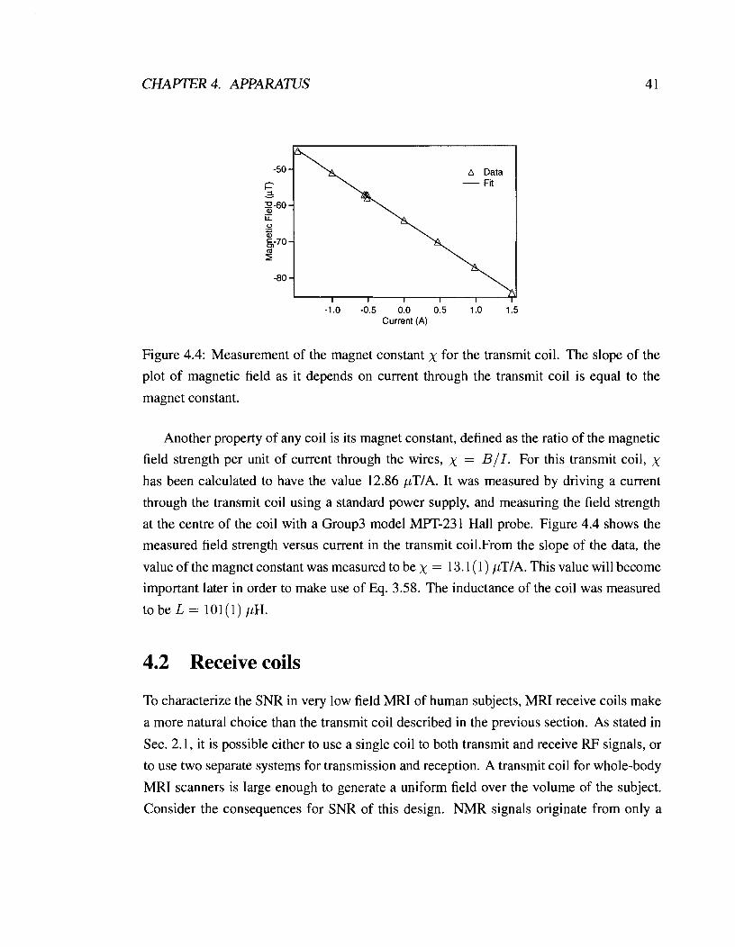
CHAPTER 4. APPARATUS
-1.0 -0.5 0.0 0.5 1.0 1.5 Current (A)
Figure 4.4: Measurement of the magnet constant x for the transmit coil. The slope of the
plot of magnetic field as it depends on current through the transmit coil is equal to the
magnet constant.
Another property of any coil is its magnet constant, defined as the ratio of the magnetic
field strength per unit of current through the wires, x = B I I . For this transmit coil, x has been calculated to have the value 12.86 pT/A. It was measured by driving a current
through the transmit coil using a standard power supply, and measuring the field strength
at the centre of the coil with a Group3 model MPT-231 Hall probe. Figure 4.4 shows the
measured field strength versus current in the transmit coil.From the slope of the data, the
value of the magnet constant was measured to be x = l3.l(l) pT/A. This value will become
important later in order to make use of Eq. 3.58. The inductance of the coil was measured
to be L = 101(1) pH.
4.2 Receive coils
To characterize the SNR in very low field MRI of human subjects, MRI receive coils make
a more natural choice than the transmit coil described in the previous section. As stated in
Sec. 2.1, it is possible either to use a single coil to both transmit and receive RF signals, or
to use two separate systems for transmission and reception. A transmit coil for whole-body
MRI scanners is large enough to generate a uniform field over the volume of the subject.
Consider the consequences for SNR of this design. NMR signals originate from only a

CHAPTER 4. APPARATUS 42
small region of the sample (i.e. the excited slice) while the noise originates from the entire
sample. A transmit coil is thus sensitive to noise from the entire sample and has a poor
SNR. If we consider the filling factor 7, defined as the ratio of the volume of the region
being imaged to the sensitive volume of the coil, we see that a transmit coil has a low filling
factor.
Commonly, SNR can be improved by using a higher filling factor coil. This can be done
with a separate receive coil (or coils) that is smaller (than the transmit coil), sits very close
to the sample, and is most sensitive to spins near the surface of the sample. Consequently,
this design is also most sensitive to noise from nearby spins rather than the entire sample.
Measurements obtained from receive coils with larger 7 therefore have a higher SNR than
those obtained with lower 7 transmit coils.
For the experiments described in this thesis the main receive coils used by Bidinosti
et al. [3,4] were duplicated: two 32 cm x 40 cm rectangular wooden formers were wound
with ten turns each of stranded, insulated 18 AWG copper wire to create our prototype.
Hence the total length of wire is - 30 m. Stranded wire was used to partially avoid the skin
effect described in Sec. 2.4. To more effectively reduce the skin effect, Litz wire could be
employed. The two coils were connected in series and arranged in front and in back of the
subject's thorax, separated by 28 cm. A drawing of these coils is shown in Fig. 4.5. The
inductance of the coils when connected in series was measured to be 197.3(1) pH.
4.3 Loss measurement circuitry
Ohmic losses in samples can be measured by detecting their loading effect on a resonant
circuit (see Chapter 5). To create a resonant circuit, the coil relevant to the appropriate
experiment - either the transmit coil or the receive coil pair - was used as the inductor, and
tuned with an adjustable air gap capacitor.
We chose to excite the resonance indirectly by driving an alternating current through
a small coil which is weakly inductively coupled to the resonant circuit. Similarly, the
response of the circuit was detected with a pair of weakly coupled receive coils. Using
this configuration of separate coupling loops for drive and detection allows the resonance
to be measured in transmission. That is, the drive loop transmits signal to the detection
loop almost exclusively via their coupling to the transmit coil. This can be contrasted to

CHAPTER 4. APPARATUS
Wooden Formers
Front View End-On View
Figure 4.5: Illustration of the receive coils used when measuring losses in human subjects.
The small drive (DRV) and detection (DET) coils that are shown here are discussed in
Sec. 4.3.
reflection measurements in which one coupling loop is used to both drive and detect the
resonance. The benefit of a transmission measurement is that far from resonance, the signal
in the detection loop is zero, whereas the signal from a reflection measurement is not.
Three nine-turn coils with a 4.75 cm diameter were used as coupling loops; one of
which served as the drive loop (DRV) while the remaining two were connected in series
to form the detection loop (DET). The two coils in the detection loop were counter-wound
with respect to eachother to reduce undesirable direct coupling between DRV and DET. For
experiments involving the transmit coil, the drive and detection loops were coupled to the
transmit coil by positioning them such that the B1 field lines pass perpendicularly through
their cross sectional area as shown in Fig. 4.6. When using the receive coils, the drive
and detection loops were coupled to one of the receive coils as shown in Fig. 4.5. Again,
this arrangement allows the field lines produced by the receive coil to pass perpendicularly
through the coupling loops. Additionally, DRV and DET were placed in perpendicular

CHAPTER 4. APPARATUS
DET . DRV
Figure 4.6: Schematic diagram of transmit coil (centre), tuning capacitance (C), drive loop
(DRV, right) and detection loops (DET, left). The coupling of the B1 field lines to the de-
tection loops is shown in the detail. Drawings copyright Mike Hayden (2006). Used with permission.

CHAPTER 4. APPARATUS
Figure 4.7: Circuit used to measure the effective resistance of a sample. A small coil L1 is
used to drive current in the resonant cavity, the LRC circuit on the right. The induced EMF
in the receive coils L3 is measured with a preamplifier and a lock-in amplifier.
planes to further reduce direct coupling, as can be seen in Fig. 4.5.
To conduct measurements of the quality factor of the tuned coil, the apparatus were
arranged as described above. The drive loop was driven with a function generator (FG),
in series with a dropping resistor Rd to maintain a constant current in the drive coil. The
voltage across the detection coils was detected with a preamplifier followed by a phase
sensitive detector (also called a lock-in amplifier). The apparatus may be modeled with the
circuit shown in Fig. 4.7. The inductors L1, L2 and L3 represent the drive, resonant, and
detection coils respectively; R1, R2 and R3 represent their resistances. The M's repesent
the mutual inductances: MI2 is that between the drive loop and L2, MZ3 between L2 and
the detection loop, and M13 between drive and detection loops directly. The capacitances
C1 and C3 represent the capacitances of the cables and instruments used in the experiment,
while C2 is the tuning capacitance. Each of these quantities (except for R2), including the
frequency dependence of R1 and R3, were measured directly using standard techniques.
The resistance R2 is the quantity that is extracted from measurements of the quality factor
of the resonance.

CHAPTER 4. APPARATUS
Field mapping coil and circuitry
Measurements of the magnetic field inside the transmit coil were obtained using a small
probe coil. The probe coil has a self-resonance at - 1 MHz, has 28 turns and is 2.1 cm in
diameter. This is small enough compared to the size of the sphere to be considered a point
probe for the purposes of the experiment. The size of the sphere is the relevant length scale
because it appears in the expressions for the magnetic field (Chapter 3). To estimate the
error introduced by this assumption, the full integral of the magnetic flux over the area of
the probe coil was calculated under typical conditions. The calculation shows that the finite
size of the probe coil reduces the measured magnetic field by no more than 0.5%.
To repeatably position the probe coil, a wooden jig was secured to the top of the transmit
coil. The jig can be rotated to be at any azimuthal angle. The uncertainty in the angle is
estimated to be - 0.5".
The probe coil was mounted on the end of a long hollow plexiglass rod which passed
through a slot and was clamped in place such that it was in the xz-plane of the transmit
coil for all the measurements. This arrangement is illustrated in Fig. (4.Q which shows a
drawing of the apparatus and a photograph representing the experiment.
To place the probe coil into the xz-plane, the EMF induced across the probe coil was
measured while scanning its vertical position - f 2 cm from the equator of the sphere. The
variation in the signal was - 5%, indicating that the sensitivity to the vertical position is
quite high. The probe coil was placed in the plane of the equator of the sphere by adjusting
the vertical position of the probe coil until the signal amplitude was a maximum. It is
estimated that the vertical position of the probe coil is within -0.5 mm of the equator of the
sphere. The radial position of the probe coil within the xz-plane, relative to the centre of
the sphere, was determined by measuring the distance from the sphere equator to the inner
wall of the transmit coil, along the axis of measurement. This distance was measured to
a precision of 0.5 mm. Additionally the outer diameter of the sphere in the xz-plane was
measured to determine the distance between the probe coil and the isocentre of the transmit
coil. Slight deviations in the shape of the phantom from a true sphere however prevent us
from determining the accuracy of the position of the probe coil at the 0.5 mm level. Rather,
given that the uncertainty in the mean sphere radius is -0.3 mm, the relative positioning of
the coil is more likely accurate to -1 mm. Furthermore, the diameter of the transmit coil

CHAPTER 4. APPARATUS
Figure 4.8: Left: Drawing of the apparatus used for measuring the oscillating magnetic field
inside the transmit coil. The outer cylinder represents the transmit coil former (windings
are not shown). The probe coil is mounted on a rod passing through a slot in an alignment
jig on the top of the transmit coil form. The jig may be oriented in any direction about
the cylinder axis and the probe coil may be rotated in any direction about its axis. Right:
Photograph indicating arrangement of the probe coil (on the left) relative to the phantom (on
the right). The glass flask is representative of the phantom, although a different phantom
was actually used in the experiment (see Sec. 4.5).
CHAPTER 4. APPARATUS
former varies as a function of angle by -5 mm, but this variation was taken into account in
the determination of the coil position.
In this experiment the transmit coil was not driven with the DRV coil or tuned with an
external capacitor, but rather was driven via a direct connection to the secondary windings
of a transformer; the FG being connected across the primary windings. In this way a larger
oscillating field is generated inside the transmit coil. The reason for including the trans-
former - rather than having a direct connection between the FG and transmit coil - is to
reduce electric field effects arising from the fact that each of the wires in the transmit coil
is at a slightly different potential. Therefore the transmit coil acts as a collection of weak,
oscillating electric multipoles. Consider two distinct effects associated with the electric
fields generated by these multipoles: (i) the capacitive coupling between the probe coil and
the transmit coil serves as a mechanism for the oscillating electric fields to impose potential
differences across the probe coil; (ii) the electric fields drive both free and bound charges
in the sample. Each one of these effects influences the measurement.
The reason for including the transformer becomes apparent if we consider the potentials
involved in the experiment. Since the function generator provides an oscillating potential
that is referenced to ground, if it is connected directly across the transmit coil, one end
of the coil windings is grounded. Thus the mean potential of the transmit coil is forced
to swing from negative to positive with each period of oscillation. This large asymmetric
potential swing causes capacitively coupled EMFs to appear across the probe coil, unless
an isolation transformer is used. Additionally, a centre-tap was employed to ground the
midpoint of the windings to ensure that the potential is evenly balanced between the two
halves of the transmit coil. An improved transmit coil could be made by interleaving the
windings of the saddle coils to further reduce the electric multipole fields inside the transmit
coil.
Evidence for reduction of the electric fields inside the transmit coil was observed by
performing two types of measurements, before and after the changes described above were
made. First, using a short electric dipole antenna, the electric field within the transmit coil
was directly measured. Second, the change in the EMF across the probe coil was monitored
as the empty fibreglass container (i.e. a sample of nominally lossless dielectric) was placed
inside the transmit coil. When the FG was connected directly across the terminals of the
transmit coil, the magnitude of the EMF across the probe coil was observed to change by

CHAPTER 4. APPARATUS
Transmit Coil Preamplifier
Probe Coil
Transformer
Figure 4.9: Instruments and circuitry used to measure the field in the vicinity of the sphere.
The transmit coil was grounded at the centre of the windings. The signal from the function
generator was used to drive a transformer, connected directly to the transmit coil. These
attempts to balance the drive circuit reduce capacitive coupling effects in the probe coil.
a maximum of - 1 % when the empty fibreglass container was placed inside the transmit
coil. When the FG was floated and the midpoint of the transmit coil was grounded, the
change in the EMF was reduced to - 0.1 %, which is at the same level as the noise in the
measurement. We therefore infer that the balancing of the electric potential between the two
halves of the coil reduced capacitive coupling effects to the probe coil by a factor of ten.
Furthermore, magnetic field perturbations due to the dielectric container are not measurable
after this procedure was done. While these observations do not tell us if electric fields are
responsible for driving significant currents in the conducting sphere, it is possible to make
arguments based on dimensional analysis that such effects should be much smaller than
magnetically induced losses [l 11.
The circuits involved in the field mapping measurement are illustrated in Fig. 4.9. In this
experiment we may still refer to transmitting and receiving signals; the function generator
drives the transmit (B1) coil (via the transformer) and the circuit response is detected with
the probe coil. Therefore 'transmit' in this experiment refers to the transmit (B1) coil and
'receive' refers to the probe coil.

CHAPTER 4. APPARATUS 50
[ Sphere # I Approx. Volume (L) I Radius(m) / Material I Used in
1 1 1 10 1 0.137(1) 1 glass flask / loss I 2
3
Table 4.1: Characteristics of the phantoms used in these experiments. The 'loss' refers to
the measurement of ohmic losses in spherical samples (Sec. 5.1) and the 'field map' refers
to the measurement of the magnetic field near the sphere (Sec. 5.2).
4
5
4.5 Phantom preparation and placement
7
5
All of the phantoms used in this experiment were spherical containers filled with NaCl
solutions. One of these containers was made by coating a rubber ball with fibreglass and
then drilling holes for filling and draining. This particular phantom was used both in the
measurement of losses and the measurement of magnetic field perturbations. When the
loss experiment was expanded to include the dependence on the sphere radius, additional
roundbottom Pyrex glass flasks of varying radii were used. A list of the properties of the
phantoms and their functions is provided in Tab. 4.1. The uncertainties in the sphere radii
represent measured deviations from non-uniformity.
The use of NaCl solutions is appealing because they are cheaply and readily prepared,
and the electrical conductivity is readily deduced from tables of published data [77]. The
concentration of the solution used in this work was approximately 2.3 M, because a mea-
surable effect was seen when the fibreglass container was filled with a solution of this
concentration.
Independent determinations of the conductivity of solutions were performed in two
ways. The first calculation uses the mass of salt and the mass or volume of water used
to prepare the solutions. The molarity M of the solution is determined from these values:
2
1
where ms is the mass of salt used (in grams) and V is the volume of the solution. Two
solutions were prepared. One was prepared by weighing the mass of salt and the mass of
0.1 18(1)
0.1 08(1)
0.0788(2)
0.063 l(2)
fibreglass
glass flask
loss and field map
loss
glass flask
glass flask
loss
loss
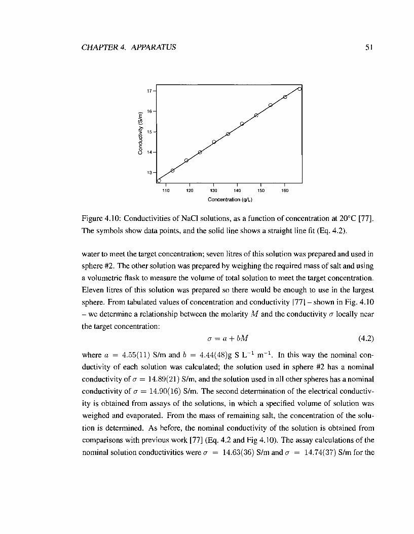
CHAPTER 4. APPARATUS
Concentration (dL)
Figure 4.10: Conductivities of NaCl solutions, as a function of concentration at 20•‹C [77].
The symbols show data points, and the solid line shows a straight line fit (Eq. 4.2).
water to meet the target concentration; seven litres of this solution was prepared and used in
sphere #2. The other solution was prepared by weighing the required mass of salt and using
a volumetric flask to measure the volume of total solution to meet the target concentration.
Eleven litres of this solution was prepared so there would be enough to use in the largest
sphere. From tabulated values of concentration and conductivity [77] - shown in Fig. 4.10
- we determine a relationship between the molarity M and the conductivity a locally near
the target concentration:
a = a + b M (4.2)
where a = 4.55(11) S/m and b = 4.44(48)g S L-' m-l. In this way the nominal con-
ductivity of each solution was calculated; the solution used in sphere #2 has a nominal
conductivity of a = 14.89(21) S/m, and the solution used in all other spheres has a nominal
conductivity of a = 14.90(16) S/m. The second determination of the electrical conductiv-
ity is obtained from assays of the solutions, in which a specified volume of solution was
weighed and evaporated. From the mass of remaining salt, the concentration of the solu-
tion is determined. As before, the nominal conductivity of the solution is obtained from
comparisons with previous work [77] (Eq. 4.2 and Fig 4.10). The assay calculations of the
nominal solution conductivities were a = 14.63(36) S/m and a = 14.74(37) S/m for the
CHAPTER 4. APPARATUS
solutions used in sphere #2, and all others, respectively.
The two values of conductivity obtained for each solution can be averaged to yield
a 'preparation' conductivity. For the solution used in sphere #2, we obtain a value of
- 14.76(21) Slrn. For the solution used in all other spheres, we obtain a value of aprep - - 14.82(20) Slrn. Since these two values overlap, they were averaged to give the aprep -
preparation conductivity representing the conductivity of all the spherical samples used in
this thesis. This value is a,,,, = 14.79(15) Slrn.
Note that this value of conductivity allows us to calculate the skin depth b of the sam-
ples. At a frequency of 10 kHz, the skin depth is 6 = 1.3 m, while at 1 MHz the skin depth
is 6 = 13 cm. For the largest sphere (#I) at 1 MHz, the skin depth is the same size as the
radius of the sphere. In other cases, the skin depth is much larger than the radius. This
situation allows us to probe the thin limit up to the point where a - b.
Several additional details regarding the preparation and assay of solutions are listed
below.
Adsorbtion and absorption of water vapour onto the glassware and into the salt re-
spectively were determined to have a total effect of - 0.1 % on the measured salt mass.
The salt was not baked prior to being weighed. However during assays the mass of the salt
was taken while the salt and glassware were still hot.
The temperature of the water used to prepare the solution for sphere # 2 was not
recorded. The temperature of the water used to prepare the solution for other spheres was
20.0(1)", consistent with the data used from the CRC handbook [77]. Therefore tempera-
ture variations were not accounted for in the values of the concentrations a,,,, for either
solution.
Variations in the solution temperature during experiments due to changes in the ambi-
ent temperature were included by considering a 2.5" temperature uncertainty to contribute
to the uncertainty in the concentration a,,,, for both solutions.
Repeatable, centred placement of the fibreglass sphere inside the transmit coil was
achieved using an annular disc of foam fitted around the sphere. The diameter of the disc
matched the inner diameter of the coil form, and a section of the disc was cut away to
make room for the probe coil. The sphere was moved into position using a rope and pulley
system. In other cases the sphere was placed on a platform inside the transmit coil and
centred to within - 1 cm by measuring the distance to the transmit coil walls. Placement

CHAPTER 4. APPARATUS 5 3
at the exact isocentre during the loss measurement is not necessary given the homogeneity
of the transmit coil. Recalling Fig. 4.3, we can see that a 1 cm error in the xz-plane of the
placement of a sphere having a - 12 cm radius causes the magnetic field to vary by less than
0.5 % over the volume of the sphere. For the field measurement however, the measurement
is very sensitive to the relative placement of the sphere and probe coil, and that is why the
centring disc was used. The vertical position was set by aligning the edge of the foam with
a fiducial mark on the inside of the transmit coil wall, to within - 2 mm.
4.6 Data acquisition
In both the loss measurement and the field mapping measurement, a transmit coil needs to
be driven with a current, and the signal across a receive coil needs to be measured. In both
cases, the driving current was provided by an Agilent 33120A function generator and the
signal in the coil was measured using a preamplifier (either Princeton Applied Research
model 11 3 or Stanford Research Systems model 560) followed by an EG & G PAR model
5202 lock-in amplifier which allows for phase-sensitive detection. The lock-in outputs
were fed into two HP model 3457A digital multimeters (DMMs). The transmit and receive
circuits are shown in Fig. 4.1 1.
The resonance measurements were automated using a GPIB interface to connect the
instruments to a computer (PC). LABVIEW software was written to control the function
generator drive frequency and capture the DMM measurements of the lock-in outputs (the
lock-in did not have GPIB capabilities). The frequency sweep must be broad enough to
capture the essential features of the resonance curve, including the resonance peak and the
outer 'wings'. Scans were typically 7-15 times the width of the resonance peak, depending
on the resonance frequency. It is important to collect the entire frequency scan relatively
quickly for two reasons. First, the resistance of the coil includes effects due to electromag-
netic coupling with its environment, which is subject to change. The resistance of the coil
has also been observed to vary with the ambient temperature in a manner consistent with the
temperature dependence of the resistivity of copper. Specifically, a change in the resistance
of - 1 % is seen to correlate with a temperature change of - 1 %, from which we conclude
that dR/R - dT/T. Because of these two effects, the time between scans must not be so
great that a measurable change the resistance occurs due to these factors. Second, when

CHAPTER 4. APPARATUS
Transmit or DRV Coil
DET probe
Reference I I I I I I
1 PC p + . j ~ y coil
DET Coil
Figure 4.1 1 : Schematic illustration of computer control used in the experiments. Top: The
current in the transmit coil was driven with a function generator. Middle: The signal in
the receive coils or probe coil was amplified first with a pre-amplifier, then with a lock-in
amplifier. The in-phase (X) and out-of-phase (Y) components of the signal were measured
with digital multimeters. Bottom: Block diagram of the computer control. During mea-
surements of the resonance curve, the function generator was computer-controlled and the
reading on each DMM was recorded by computer using a GPIB interface.
Preamp Lock-in
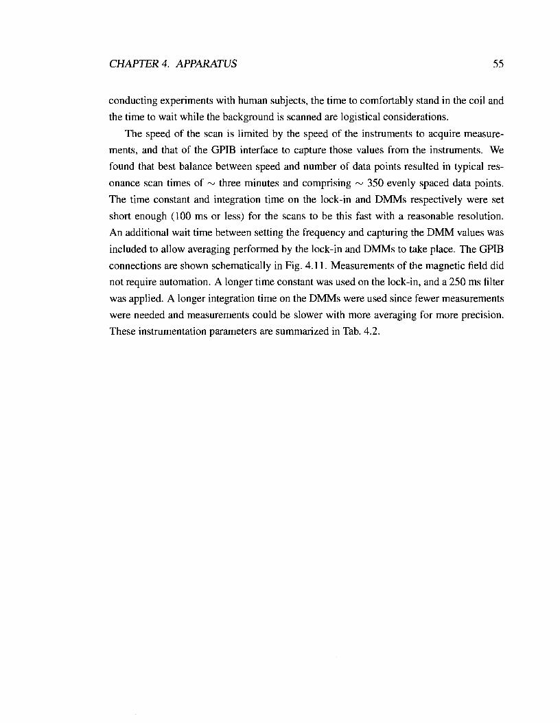
CHAPTER 4. APPARATUS 55
conducting experiments with human subjects, the time to comfortably stand in the coil and
the time to wait while the background is scanned are logistical considerations.
The speed of the scan is limited by the speed of the instruments to acquire measure-
ments, and that of the GPIB interface to capture those values from the instruments. We
found that best balance between speed and number of data points resulted in typical res-
onance scan times of - three minutes and comprising -- 350 evenly spaced data points.
The time constant and integration time on the lock-in and DMMs respectively were set
short enough (100 ms or less) for the scans to be this fast with a reasonable resolution.
An additional wait time between setting the frequency and capturing the DMM values was
included to allow averaging performed by the lock-in and DMMs to take place. The GPIB
connections are shown schematically in Fig. 4.11. Measurements of the magnetic field did
not require automation. A longer time constant was used on the lock-in, and a 250 ms filter
was applied. A longer integration time on the DMMs were used since fewer measurements
were needed and measurements could be slower with more averaging for more precision.
These instrumentation parameters are summarized in Tab. 4.2.
CHAPTER 4. APPARATUS
when measuring resonance: sphere #2
lock-in time constant: 100 ms
wait time between measurements: 500 ms
DMM averaging time (multiples of 1/60): 1
when measuring resonance: all other spheres
lock-in time constant: 100 ms
wait time between measurements: 500 ms
DMM averaging time (multiples of 1/60): 1
when measuring fields: sphere #2
lock-in time constant: 100 ms
lock-in filter: 250 ms
DMM averaging time (multiples of 1/60): 10
when measuring resonance: humans
lock-in time constant: 10 ms
wait time between measurements: 100 ms
DMM averaging time (multiples of 1/60): 1
Table 4.2: Instrumentation settings during each of the experiments. The speed at which the
experiment can be performed depends on these values.

Chapter 5
Methods
In this chapter I describe two experimental techniques used to study weakly conducting
samples: (i) the measurement of losses associated with induced currents in samples and (ii)
the measurement of magnetic fields associated with the induced currents in a sample. The
procedures to collect the data and the methods employed to analyze the data are presented.
5.1 Measurement of ohmic losses
The sample resistance of spherical phantoms and human subjects was measured at low
frequencies by characterizing the perturbation to the quality factor of a tuned LRC circuit.
The change in the quality factor due to the presence of the sphere is proportional to the
effective sample resistance.
Figure 5.1 shows an LRC circuit, which consists of lumped resistive (R), capacitive
(C), and inductive (L) elements that are driven by a sinusoidal voltage of amplitude V and
angular frequency w. The drive voltage is represented by the complex phasor V = Ve-i"t.
The total impedance viewed by the source is
which has a magnitude

CHAPTER 5. METHODS
Figure 5.1 : A series LRC circuit.
that is minimum at the resonance frequency
The current in the circuit is represented by the complex phasor I = Ie-iwtse and is given
bv Ohm's Law
The time-average power dissipated by the circuit is
which reaches a maximum when w = wo:
The bandwidth of the resonant circuit is defined as

CHAPTER 5. METHODS 5 9
where w+ and w- are the frequencies at which the power has dropped to half of its maxi-
mum value (in the positive and negative directions from the peak value, respectively). These
points are given by the solution to
The quality factor, defined as
provides a measure of the sharpness of the resonance. In the case of weak damping
(R << wL), the bandwidth is Aw = RIL, which leads to
At resonance, the magnitude of the voltage across the resistor is V, while the magnitude of
the voltage across both the inductor and capacitor is VQ.
When a sample of material is allowed to interact with the electromagnetic fields gen-
erated by the circuit elements, the response of the circuit is perturbed in a manner that
depends on the electromagnetic properties of the sample. In particular, as is the case for the
work described in this thesis, the perturbation to the quality factor can be modeled as an
effective sample resistance R, in the circuit. If the perturbation is small, the quality factor
is decreased to -
The values of wo and Q are determined from measurements of the unloaded circuit. If the
circuit is re-tuned to the same resonance frequency after addition of the sample (by adjusting
the tuning capacitor), a second measurement of the loaded quality factor Q' allows Eq. 5.15
to be applied directly to determine R,. Figure 5.2 shows an example of two resonant curves
with the same resonant frequency but different quality factors.
5.1.1 Procedure
To measure R,, two separate measurements of the quality factor Q are needed: one when
the circuit is unloaded, and one when the circuit is loaded by the sample. To obtain these

CHAPTER 5. METHODS
0.47 0.48 0.49 0.5 0.51 0.52 0.53 0. Frequency (kHz)
Figure 5.2: Calculated examples of the magnitude of the current (Eq. 5.5) in a series LRC
circuit, in the vicinity of resonance. The dashed curve is for a circuit with a larger resistance
and hence smaller quality factor than the circuit represented by the solid line.
measurements, we made a resonant circuit using transmit coil and additional circuitry de-
scribed in Sec. 4.3. The resonant behaviour of the circuit was characterized in transmission.
The EMF across the receive coils was measured while sweeping the frequency of the drive
current through the resonance.
The procedure to collect data was as follows. The tuning capacitor was adjusted to
set the circuit to the desired resonance frequency, then the voltage across the receive coils
was measured over a frequency range centred on the resonance frequency (usually several
times the bandwidth). The data were curve fit to a model function - presented in the next
section - yielding the resonance frequency and the resistance of the circuit. Upon the
additiontremoval of the sample intotfrom the coil, both properties are changed. The tuning
capacitor was then adjusted to match the resonance frequency of the previous run as closely
as possible, and the resonance was scanned and curve fit again. The scan when the coil
was empty is called the 'background' scan and the scan when the sample is present inside
the coil is called the 'foreground' scan. The difference in resistance between foreground

CHAPTER 5. METHODS 6 1
and background scans determines the value of Rs at the given resonance frequency.' This
procedure was then repeated at a number of discrete resonance frequencies over the range
0.1 - 1.25 MHz to determine the frequency dependence of Rs.
5.1.2 Method of data analysis
A simple expression for the voltage expected at the input to the preamplifier can be esti-
mated as follows. Recalling the impedance seen by the source, (Eq. 5.3) and Ohm's Law
(Eq. 5.5), the magnitude of the current in the circuit is
As described in Sec. 4.3, the resonant circuit was driven inductively, rather than directly as
shown in Fig. 5.1. Therefore, the magnitude of the EMF induced across the inductor (and
hence the LRC circuit) is
where v is the voltage across the drive loop, and ID is the current in the drive loop. Therefore
the magnitude of the current in the resonant circuit is related to V by Ohm's Law
V W Icx ,
Now consider the detection loops. The EMF vo across the detection loops is given by

CHAPTER 5. METHODS
Figure 5.3: Left: An example of resonance data amplitude (normalized such that '1' rep-
resents full scale) and the curve fit to the simple model function, Eq. 5.19. Right: The
residuals resulting from this fit are clearly not random.
where a is a scale factor describing the proportionality.
By fitting the resonance curves to Eq. 5.19, the values of a, R and fo = wo/(2.rr)
are obtained by letting them be free parameters in the fit. The argument presented above
allowed us to quickly obtain a model function for the data that captures all the important
features; however systematic residuals (the fit values subtracted from data values) from
these fits were observed. For example, Fig. 5.3 shows a background data set 750 kHz, the
curve fit to Eq 5.19, and the residuals that result from the fit. Generally, we see there is
a slight overall mismatch between the data and fit - the fit tends to undershoot on the low
frequency side of resonance and overshoot on the high frequency side. The feature at the
centre of the scan is associated with the resonance. I pointed out that the voltage across the
inductor and capacitor are multiplied by Q at the resonance. Small deviations of the circuit
from the model become amplified near the resonance by this effect. Any inadequacies of
the circuit model to describe the real apparatus will tend to play a more important role near
resonance and so the fit function will tend to describe the data more poorly. Notice that the
width of the feature visible in Fig. 5.3 is - 10 kHz while the width of the resonance is - 'While R, and R,,il each in fact depend on frequency, we are ignoring variations of their values over the
width of the resonance scan. Inclusion of the appropriate frequency dependence influences the resulting fit
values by approximately 0.05 %.

CHAPTER 5. METHODS
Figure 5.4: Circuit diagram of the model circuit used to model our resonance apparatus.
The various components are defined in Sec. 4.3.
7 kHz. The size of the residuals is approximately on the 1 % level. This is not particularly
large but the systematic nature of the residuals indicates that a more realistic model function
is required if we are to reliably and accurately detect and monitor small perturbations of the
resonance curve. In an attempt to reduce the residuals of the fits to the data, I conducted
a more in-depth analysis of the circuits involved in the apparatus. This analysis is now
presented.
General case
A detailed model for the electrical circuit was presented in Sec. 4.3. For convenience, the
circuit diagram is shown again in Fig. 5.4. Recall that R2, L2 and C2 represent the compo-
nents of the resonant circuit. Thus R2 is the quantity that will ultimately be measured. We
begin by defining the following symbols to simplify the notation.

CHAPTER 5. METHODS
Impedance of drive coupling loop: Z1 = R1 + iwLl
Resonance frequency: wo = l / d m Impedance of circuit 2: Z2 = R2 + iwL2 1 - 3 ( "'1
Input impedance of preamp: ZL = R L / ( l + iwRLC3)
Impedance of circuit 3: Z3 = R3 + iwL3 + ZL
The overall eciWt time dependence present in the phasors V and I propagates through
the analysis of the circuit, and will be suppressed to simplify the notation. It is important
to note that these factors are still complex quantities and that the relative phase between V
and I is significant.
For circuit 1 (the drive circuit), the Kirchoff voltage equation may be written as:
where I; is the current through the resistor Rd and is determined from a second Kirchoff
voltage equation for this circuit
I l z l - iw(M1212 + M1313) = (1; - I1)Zcl , (5.21)
where Zcl = - i /(wC1) is the impedance of the capacitance C1. Combining Eqs. 5.20 and
5.21, we have, for circuit 1
Rd v = ( 1 1 2 1 - i w ( M d 2 + ~ 1 3 1 3 ) ) ( 1 + -) + 11% , (5.22)
Zc1 while the circuit equations describing circuits 2 and 3 require that
0 = 12Z2 - iw(M12I1 + M2313) (5.23)
0 = 13Z3 - iw(M1311 + M2312) . (5.24)
The magnitude of the voltage at the preamp input is given by
and I3 is found by solving Eqs. 5.22, 5.23, and 5.24. One way to write the solution in a
compact form is to define the following quantities
A = Rd + Zci
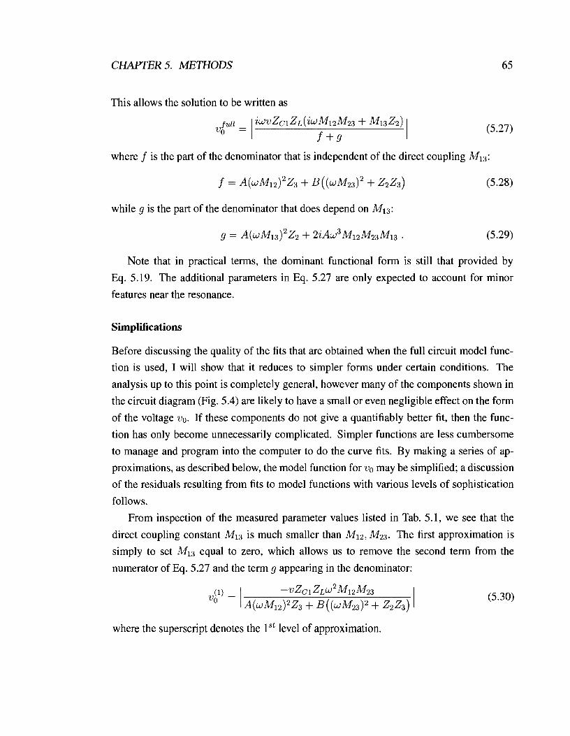
CHAPTER 5. METHODS
This allows the solution to be written as
,y = i ~ v Z c i Z ~ ( i ~ M i z M 2 3 + Mi3Zz) (5.27) f + g
where f is the part of the denominator that is independent of the direct coupling Mi3:
f = A ( ~ M l z ) ~ z 3 + B((wM23)' + 2 2 2 3 ) (5.28)
while g is the part of the denominator that does depend on Mi3:
g = A ( w M ~ ~ ) ~ z ~ + 2iAw3 M~~ ~ 2 3 ~ 1 3
Note that in practical terms, the dominant functional form
(5.29)
is still that provided by
Eq. 5.19. The additional parameters in Eq. 5.27 are only expected to account for minor
features near the resonance.
Simplifications
Before discussing the quality of the fits that are obtained when the full circuit model func-
tion is used, I will show that it reduces to simpler forms under certain conditions. The
analysis up to this point is completely general, however many of the components shown in
the circuit diagram (Fig. 5.4) are likely to have a small or even negligible effect on the form
of the voltage vo. If these components do not give a quantifiably better fit, then the func-
tion has only become unnecessarily complicated. Simpler functions are less cumbersome
to manage and program into the computer to do the curve fits. By making a series of ap-
proximations, as described below, the model function for vo may be simplified; a discussion
of the residuals resulting from fits to model functions with various levels of sophistication
follows.
From inspection of the measured parameter values listed in Tab. 5.1, we see that the
direct coupling constant Mi3 is much smaller than Mi2, MZ3. The first approximation is
simply to set Mi3 equal to zero, which allows us to remove the second term from the
numerator of Eq. 5.27 and the term g appearing in the denominator:
where the superscript denotes the lSt level of approximation.
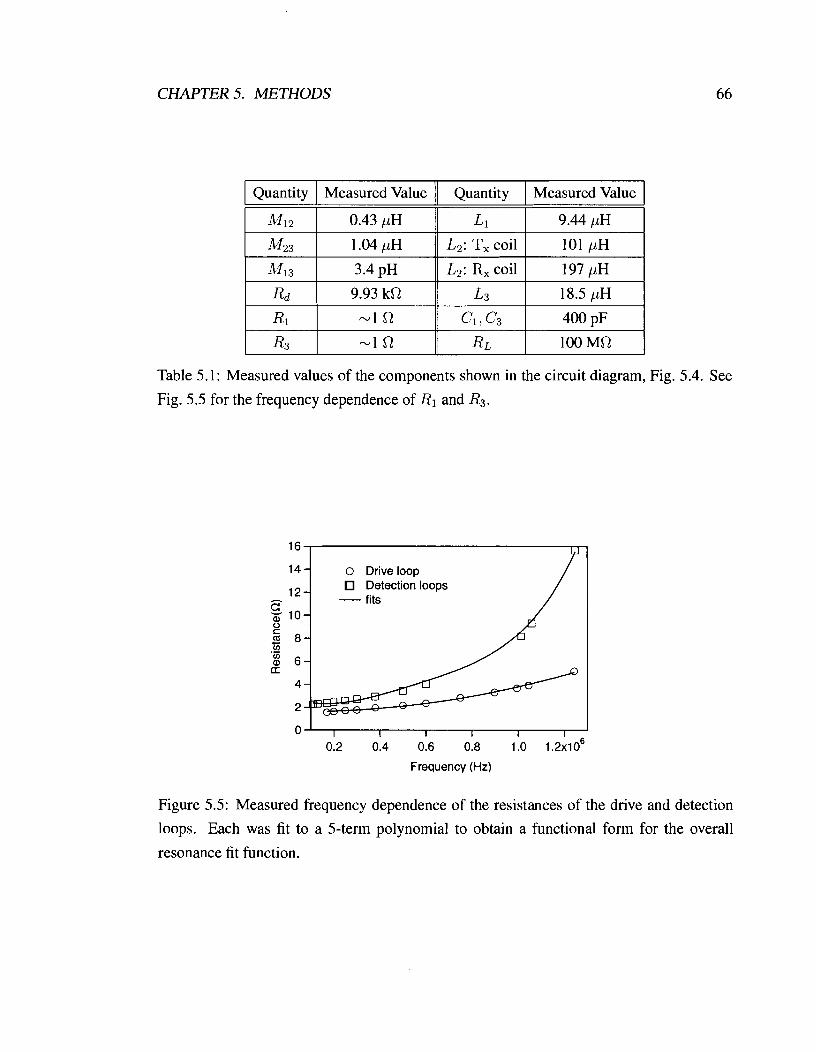
CHAPTER 5. METHODS
Quantity Measured Value
0.43 pH
1.04 pH
3.4 pH
Quantity Measured Value
-
~ 2 : Q coil I
Table 5.1: Measured values of the components shown in the circuit diagram, Fig. 5.4. See
Fig. 5.5 for the frequency dependence of R1 and R3.
0 Drive loop Detection loops
- fits - 10
0.2 0.4 0.6 0.8 1.0 1.2x10⁶
Frequency (Hz)
Figure 5.5: Measured frequency dependence of the resistances of the drive and detection
loops. Each was fit to a 5-term polynomial to obtain a functional form for the overall
resonance fit function.

CHAPTER 5. METHODS 67
Next consider the relative size of the terms in the denominator of Eq. 5.30 involving the
mutual inductances M12 and hf23 as compared to the term involving Z2Z3. Consider the first
term ( w M ~ ~ ) ~ + Z2Z3. Making use of the component values listed in Tab. 5.1, and knowing
that Z2 is typically of order 1 - 10 R in our apparatus, it is clear that ( ~ M 2 3 ) ~ << 2 2 2 3
and thus we may drop ( ~ M 2 3 ) ~ relative to 2223, giving
Next we substitute Eq. 5.26 into the denominator; this allows us to write it as
\ (Rd + ZC1Z3)(~2M;2 + Z1Z2) + RdZC1Z2Z3\. Again making use of the values from
Tab. 5.1, ~ ~ M 1 2 ~ << Z1Z2 and thus it may be dropped, giving
Now we recognize that Z1 << Zcl since R1 << wL1 and wL1 << l/(wC1) as
apparent from the values listed in Tab. 5.1. This yields
If we have an ideal preamplifier and negligible capacitance associated with the cables, the
impedance of C3 can be ignored relative to RL, and thus ZL = Z3 = RL and:
In this limit RL drops out; recalling that Z2 is the series combination of R2, L2, and C2, we
can use Eq. 5.3 to conclude
This function is identical to Eq. 5.19, where the previously defined scale factor is cr =
M12M23/Rd. Therefore, the complete model circuit simplifies to give the voltage that we
had predicted from a simple argument. Table 5.2 summarizes the approximations that were
necessary to arrive at this conclusion.
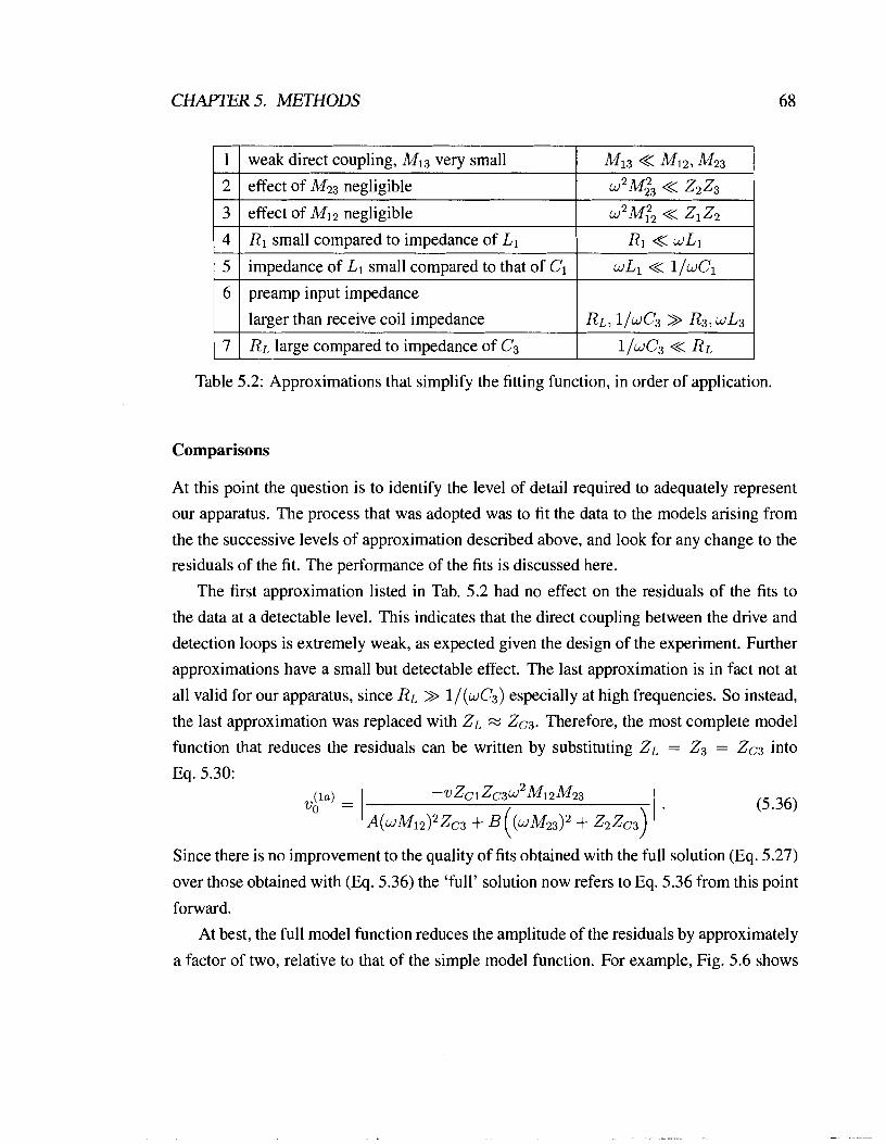
CHAPTER 5. METHODS
/ 1 ( weak direct coupling, M13 very small I M I ~ < M I ~ , M ~ ~ /
( 4 1 R1 small compared to impedance of L1 1 R1 << wL1 I
2 1 effect of M23 negligible w2 M23 << 2 2 2 3
1 7 1 RL large compared to impedance of C3 1 1 / ~ C 3 << RL I
5
6
Table 5.2: Approximations that simplify the fitting function, in order of application.
Comparisons
impedance of L1 small compared to that of Cl
preamp input impedance
larger than receive coil impedance
At this point the question is to identify the level of detail required to adequately represent
our apparatus. The process that was adopted was to fit the data to the models arising from
wL1 << llwC1
RL, 1IwC3 >> R3, wL3
the the successive levels of approximation described above, and look for any change to the
residuals of the fit. The performance of the fits is discussed here.
The first approximation listed in Tab. 5.2 had no effect on the residuals of the fits to
the data at a detectable level. This indicates that the direct coupling between the drive and
detection loops is extremely weak, as expected given the design of the experiment. Further
approximations have a small but detectable effect. The last approximation is in fact not at
all valid for our apparatus, since RL >> l / (wC3) especially at high frequencies. So instead,
the last approximation was replaced with ZL M ZC3. Therefore, the most complete model
function that reduces the residuals can be written by substituting ZL = Z3 = ZC3 into
Eq. 5.30:
Since there is no improvement to the quality of fits obtained with the full solution (Eq. 5.27)
over those obtained with (Eq. 5.36) the 'full' solution now refers to Eq. 5.36 from this point
forward.
At best, the full model function reduces the amplitude of the residuals by approximately
a factor of two, relative to that of the simple model function. For example, Fig. 5.6 shows
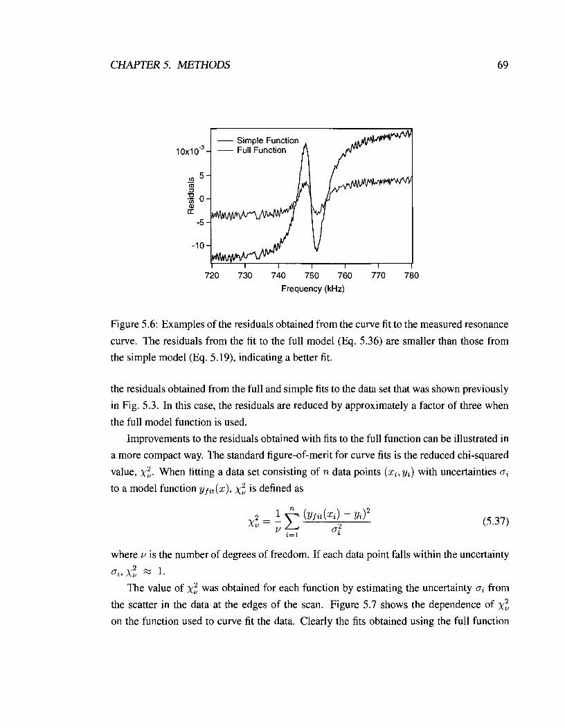
CHAPTER 5. METHODS
720 730 740 750 760 770 780
Frequency (kHz)
Figure 5.6: Examples of the residuals obtained from the curve fit to the measured resonance
curve. The residuals from the fit to the full model (Eq. 5.36) are smaller than those from
the simple model (Eq. 5.19), indicating a better fit.
the residuals obtained from the full and simple fits to the data set that was shown previously
in Fig. 5.3. In this case, the residuals are reduced by approximately a factor of three when
the full model function is used.
Improvements to the residuals obtained with fits to the full function can be illustrated in
a more compact way. The standard figure-of-merit for curve fits is the reduced chi-squared
value, x:. When fitting a data set consisting of n data points (xi, yi) with uncertainties ai
to a model function yfit(x), X: is defined as
where v is the number of degrees of freedom. If each data point falls within the uncertainty 2 ai, xv z 1.
The value of XE was obtained for each function by estimating the uncertainty ai from
the scatter in the data at the edges of the scan. Figure 5.7 shows the dependence of X:
on the function used to curve fit the data. Clearly the fits obtained using the full function

CHAPTER 5. METHODS
(
o Simple Function Full Function
0 0
0.2 0.4 0.6 0.8 1.0 1 .2x106 Frequency (Hz)
Figure 5.7: Comparison of the average X: values obtained from averaging fits to five sets
of background data. Average values obtained from fits to each of the simple and full model
functions are shown. The XE value is smaller when using the full function, indicating a
better quality of fit.
exhibit a smaller value of XE. Below - 300 kHz, the X: values from the full fit are -10;
above 300 kHz they increase to as much as lo4. In contrast, the full fit gives smaller values.
Below - 300 kHz, the XE values from the full fit are -1; above 300 kHz they increase to - lo3. Above - 300 kHz, the residuals of the fits exhibit systematic trends regardless of
which fit function is used, as clearly seen in Fig. 5.7. This is indicative that some feature of
the circuit behaviour is not captured by the models.
Another quantitative comparison between the two fits can be made by considering the
value of the resistance that is extracted from the fit. The value obtained from the full
function is not significantly different from that given by the simple fit, as can be seen in
Fig. 5.8. The difference between the sample resistances obtained from the simple and full
fit is typically less than 1 %. Much more important is the improvement in the uncertainty
in the sample resistance that is obtained when using the full fit function over the simple
fit function. Figure 5.8 also shows that the uncertainty in the value of the resistance is
typically reduced by 60 % when using the full fit. For the smaller volume samples this

CHAPTER 5. METHODS
h
X 0 0
V Sphere Number 0 1 0 2 L
Frequency (Hz)
o
0.2 0.4 0.6 0.8 1 .o 1 .2x106 Frequency (Hz)
Figure 5.8: Top: Fractional difference between the values of R, obtained from the simple
and full models. Bottom: Fractional difference between the uncertainty in values of R, obtained from the simple and full models.

CHAPTER 5. METHODS
becomes important in distinguishing the small change in resistance that occurs.
It is suspected that the residuals in these fits are a consequence of the distributed nature
of the inductance and capacitance of the B1 coil, which have been modeled here as lumped
elements. In this context, it is worth noting that the free space wavelength of electromag-
netic radiation at 1 MHz field is 300 m, which is only ten times the total length of wire in
the coil (- 30 m). As a result, at higher frequencies, the current at one end of the wire in
the coil is not perfectly in phase with the current at the other end. This effect is not mod-
eled in the circuit analysis and likely contributes to the systematic residuals. Considering
the comparison between simple and full models of the circuits, we postulate that further
improvements to the circuit model incorporating distributed elements and finite wavelength
effects might further reduce the uncertainty in R,, but that they will not likely change the
value of R, that is extracted from the data in any significant way. In spite of the small
systematic trends in the residuals, the important point remains that they are typically less
than 1 % of the signal amplitude, and that adding further complexity to the model function
is unlikely to yield significant improvements in accuracy.
Additional details
In our experiments, the recorded voltage is amplified by a preamplifier followed by a lock-
in amplifier. We may combine the effect of both amplifiers into a single gain factor and
express the measured voltage as
b m l = d f > b o l (5.38)
where the function g(f ) was characterized by measuring the output signal when a fixed,
known signal was input to the preampllock-in combination. The magnitude of all exper-
imental data were corrected by the factor g(f ) before any curve fitting was done. The
magnitude of all data were also normalized to a peak value of unity before performing
further analysis.
Another procedure that was applied to the data was to compensate for the slight mis-
match between the resonance frequencies of the foreground and background resonance
scans. Figure 5.9 illustrates how this was done. The two points in the lower part of the
sketch represent two background datapoints, at the coordinates ( f b l r Rbl) and (fb2, bf2). The
upper point represents a nearby foreground data point, ( f f , Rf). If the difference Rf - Rbl

CHAPTER 5. METHODS
Rf -------- --' + foreground I data point I I I
background data points
Rbl ----- I I
1 I
fbl f r
Figure 5.9: Definitions of quantities used to interpolate the data and correct for small fre-
quency shifts.
is used as the value of the sample resistance R,, the resulting value has a slight systematic
error due to the frequency shift. This error was reduced by interpolating the background
data to estimate the background resistance at the foreground frequency ff. A linear inter-
polation scheme was employed; this interpolated value, Ri was found by determining the
local slope b of the background data from the adjacent data point; the value of Ri at the
foreground frequency ff is
Ri = Rbl + b(ff - f b l ) (5.39)
It is worth noting that the frequency shift between foreground and background data is ex-
aggerated in Fig. 5.9. Typically the shift ff - fbl is only 0.5% of the frequency difference
fb2 - fb l between one data point and the next. In most cases, the effect of interpolation was
to change the sample resistance by 1 % of its value. In some cases, the effect was - 3-4 %,
and in rare cases the correction was as much as 8 %.
5.2 Measurement of induced magnetic field
The magnetic field in the vicinity of the sphere can be directly measured using a probe coil,
and thus can be compared with the predictions listed in Chapter. 3. This experiment was
performed using sphere # 2 (radius 12 cm) placed inside the transmit coil. In this section I
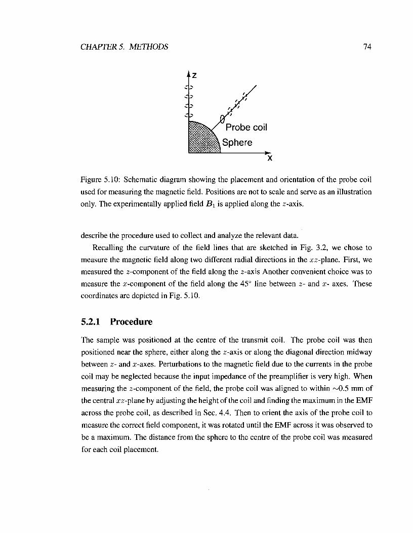
CHAPTER 5. METHODS
Figure 5.10: Schematic diagram showing the placement and orientation of the probe coil
used for measuring the magnetic field. Positions are not to scale and serve as an illustration
only. The experimentally applied field B1 is applied along the z-axis.
describe the procedure used to collect and analyze the relevant data.
Recalling the curvature of the field lines that are sketched in Fig. 3.2, we chose to
measure the magnetic field along two different radial directions in the xz-plane. First, we
measured the z-component of the field along the z-axis Another convenient choice was to
measure the x-component of the field along the 45" line between z- and x- axes. These
coordinates are depicted in Fig. 5.10.
5.2.1 Procedure
The sample was positioned at the centre of the transmit coil. The probe coil was then
positioned near the sphere, either along the z-axis or along the diagonal direction midway
between z- and x-axes. Perturbations to the magnetic field due to the currents in the probe
coil may be neglected because the input impedance of the preamplifier is very high. When
measuring the z-component of the field, the probe coil was aligned to within ~ 0 . 5 mm of
the central xz-plane by adjusting the height of the coil and finding the maximum in the EMF
across the probe coil, as described in Sec. 4.4. Then to orient the axis of the probe coil to
measure the correct field component, it was rotated until the EMF across it was observed to
be a maximum. The distance from the sphere to the centre of the probe coil was measured
for each coil placement.
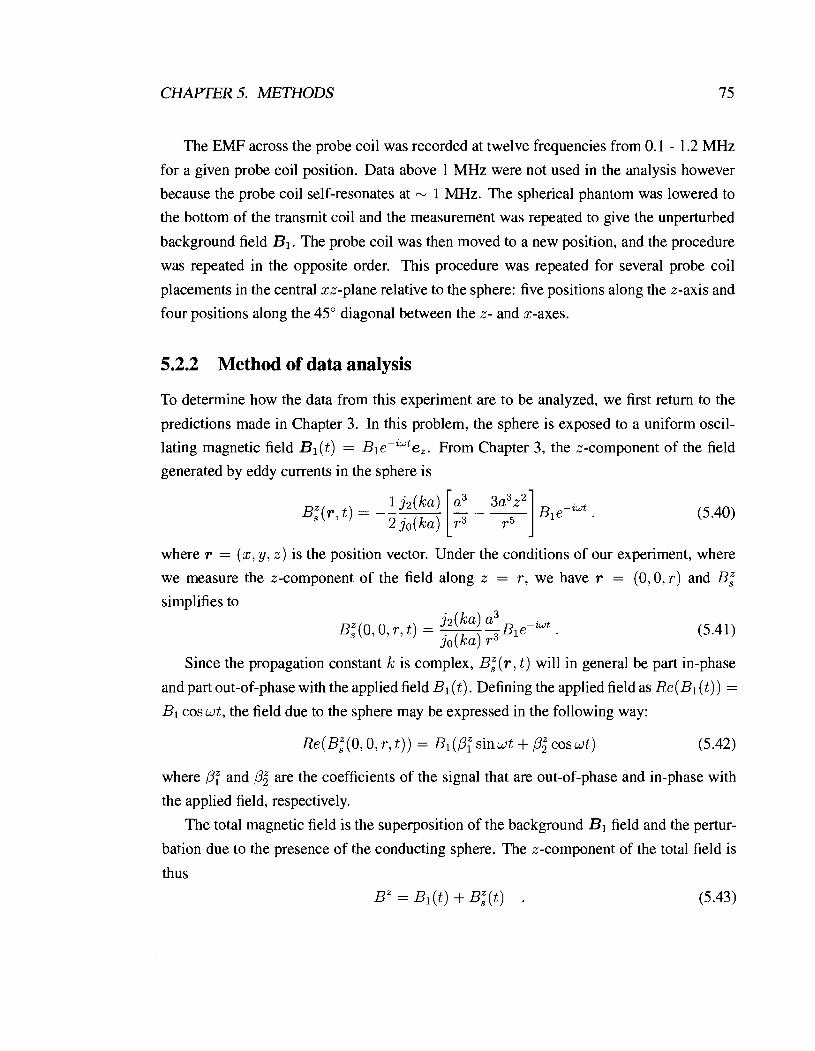
CHAPTER 5. METHODS 75
The EMF across the probe coil was recorded at twelve frequencies from 0.1 - 1.2 MHz
for a given probe coil position. Data above 1 MHz were not used in the analysis however
because the probe coil self-resonates at -- 1 MHz. The spherical phantom was lowered to
the bottom of the transmit coil and the measurement was repeated to give the unperturbed
background field B1. The probe coil was then moved to a new position, and the procedure
was repeated in the opposite order. This procedure was repeated for several probe coil
placements in the central xz-plane relative to the sphere: five positions along the z-axis and
four positions along the 45" diagonal between the z- and x-axes.
5.2.2 Method of data analysis
To determine how the data from this experiment are to be analyzed, we first return to the
predictions made in Chapter 3. In this problem, the sphere is exposed to a uniform oscil-
lating magnetic field B l ( t ) = Ble-iwte,. From Chapter 3, the z-component of the field
generated by eddy currents in the sphere is
1 ( a ) [a3 3:5z2] B;(r , t ) = --- - - - ~ ~ e - ~ ~ ~ .
2 J o ( W r3
where r = (x, y, z) is the position vector. Under the conditions of our experiment, where
we measure the z-component of the field along z = r , we have r = (O,O, r) and B,"
simplifies to
Since the propagation constant k is complex, B,"(r, t ) will in general be part in-phase
and part out-of-phase with the applied field Bl (t). Defining the applied field as Re(Bl (t)) =
B1 cos wt, the field due to the sphere may be expressed in the following way:
Re(B,Z (0, 0, r, t ) ) = B1 (P," sin wt + Pi cos wt) (5.42)
where p," and p," are the coefficients of the signal that are out-of-phase and in-phase with
the applied field, respectively.
The total magnetic field is the superposition of the background B1 field and the pertur-
bation due to the presence of the conducting sphere. The z-component of the total field is
thus
B" = Bl (t) + B,"(t) . (5.43)
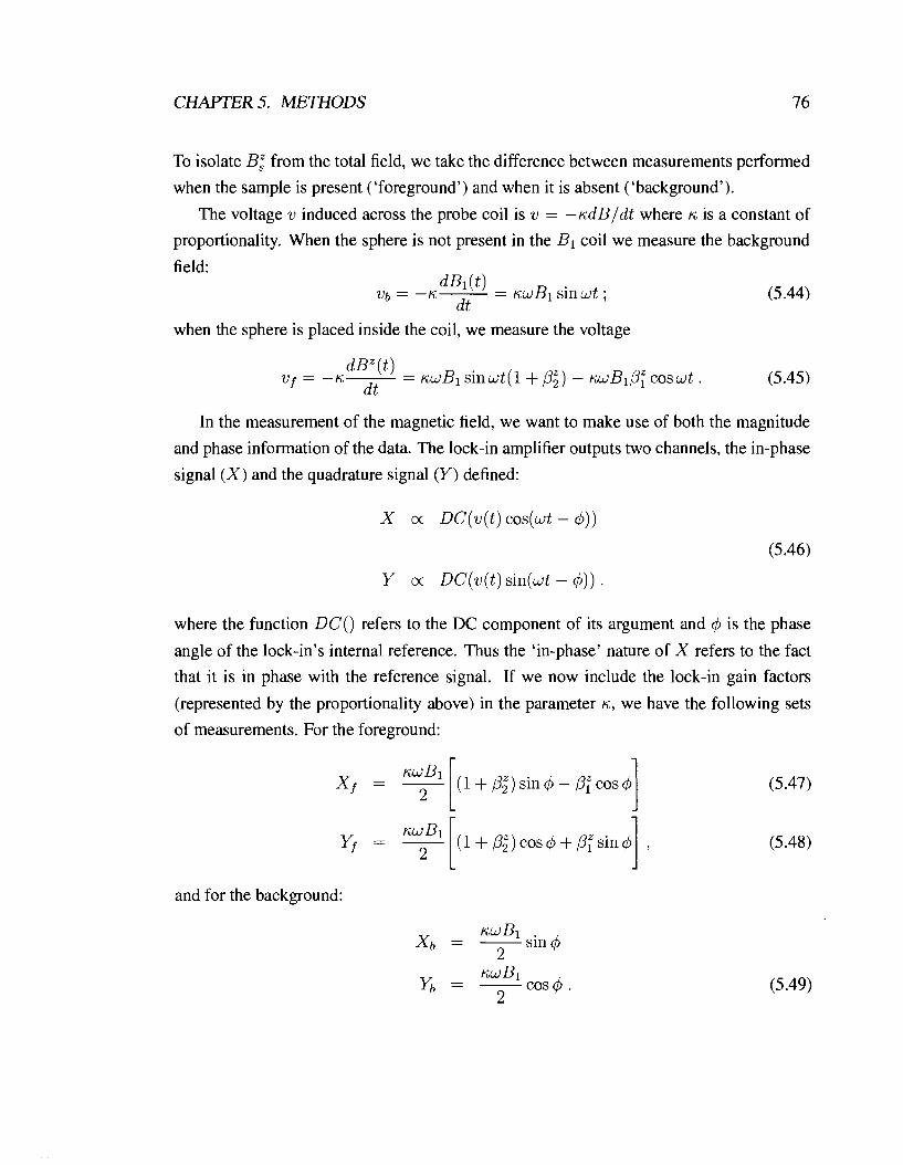
CHAPTER 5. METHODS 7 6
To isolate B," from the total field, we take the difference between measurements performed
when the sample is present ('foreground') and when it is absent ('background').
The voltage v induced across the probe coil is v = - ~ d B / d t where K is a constant of
proportionality. When the sphere is not present in the B1 coil we measure the background
field:
when the sphere is placed inside the coil, we measure the voltage
dB" (t) vf = -6- = riwBlsinwt(l + P,Z) - K W B ~ P ~ C O S W ~ .
dt
In the measurement of the magnetic field, we want to make use of both the magnitude
and phase information of the data. The lock-in amplifier outputs two channels, the in-phase
signal (X) and the quadrature signal (Y) defined:
where the function DC() refers to the DC component of its argument and 4 is the phase
angle of the lock-in's internal reference. Thus the 'in-phase' nature of X refers to the fact
that it is in phase with the reference signal. If we now include the lock-in gain factors
(represented by the proportionality above) in the parameter K, we have the following sets
of measurements. For the foreground:
and for the background:
u;wB1 Xb = -
2 sin 4
6wB1 Yb = - cos 4 .
2

CHAPTER 5. METHODS
The difference between the foreground and the background measurements are thus
We may now rearrange equations 5.50 to express and in terms of A X and AY.
An extra measurement of X6 and Yb was taken with the probe coil at the centre of the
B1 coil for each frequency and was used to determine the parameters K and 4. Denoting
these measurements X, and Y,, we may now express p,Z and p," in terms of the measured
quantities:
We now return to our spherical model (Chapter 3) and write down the predicted be-
haviour of & and p,". Recalling the power series expansion of the spherical Bessel Func-
tions presented in Chapter 3, we may write the z component of the sphere field as:
The first and second terms correspond to the parts of the field that are out-of-phase and
in-phase with the applied field, respectively. Comparing Eq. 5.54 to Eq. 5.42, we obtain the
following expressions for the coefficients P; and P," :
A similar analysis follows for the x-component of the field. The x-component of the
sphere field is
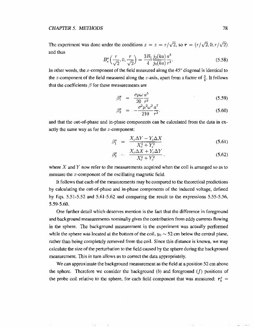
CHAPTER 5. METHODS 78
The experiment was done under the conditions x = z = I-/&, so r = (I-/&, 0, I-/&) and thus
In other words, the x-component of the field measured along the 45" diagonal is identical to
the z-component of the field measured along the z-axis, apart from a factor of 4. It follows
that the coefficients B for these measurements are
apw a5 -- Pf = ,, I-3
and that the out-of-phase and in-phase components can be calculated from the data in ex-
actly the same way as for the z-component:
where X and Y now refer to the measurements acquired when the coil is arranged so as to
measure the x-component of the oscillating magnetic field.
It follows that each of the measurements may be compared to the theoretical predictions
by calculating the out-of-phase and in-phase components of the induced voltage, defined
by Eqs. 5.51-5.52 and 5.61-5.62 and comparing the result to the expressions 5.55-5.56,
5.59-5.60.
One further detail which deserves mention is the fact that the difference in foreground
and background measurements nominally gives the contribution from eddy currents flowing
in the sphere. The background measurement in the experiment was actually performed
while the sphere was located at the bottom of the coil, yo - 52 cm below the central plane,
rather than being completely removed from the coil. Since this distance is known, we may
calculate the size of the perturbation to the field caused by the sphere during the background
measurement. This in turn allows us to correct the data appropriately.
We can approximate the background measurement as the field at a position 52 cm above
the sphere. Therefore we consider the background (b) and foreground (f) positions of
the probe coil relative to the sphere, for each field component that was measured: ri =

CHAPTER 5. METHODS 7 9
(O,yo, z ) , r j = ( O , O , z ) ; ~ , ? = ( z ,yo , r ) , r j = ( z , 0 , ~ ) . The values of P that we actually
measure are given by the difference between values measured with the sphere in these two
positions:
Substituting in the position vectors into Eqs. 5.40 and 5.58, we have
3B1 j2(ka) a3z2 B : ( T ~ ) = --
2 512 2 jo(ka) (2z2 + yo)
The relative deviation of the measurement from the value calculated earlier is
Similarly, for the x-component of the field,

CHAPTER 5. METHODS 80
For the geometry of the experiment, the size of these corrections is - -0.9 % for the z- component and -0.8 % for the x-component.
Having presented the methods to collect and analyze the data for both the measurement
of ohmic losses and the induced magnetic field in spherical phantoms, I discuss the results
of these experiments in the following chapter.
Chapter 6
Results: Spherical phantoms
In this chapter I present results from two experiments performed with the goal of measuring
the ohmic losses and magnetic field associated with eddy currents induced in spherical
phantoms. Experimental results are compared to predictions derived in Chapter 3. These
experiments function as controls to characterize the apparatus in detail; having done so,
experiments involving human subjects become possible.
6.1 Measurement of ohmic losses
In this section I present the measurements of the ohmic losses in spherical conducting
samples. As described in Chapter 5, these losses can be measured by detecting the loading
effect when a sample is introduced into a resonant circuit. Analysis of the perturbation
of the resonance curve gives the effective sample resistance R,, which is in turn related
to the power by Eq. 3.57. The sample resistance of five spheres having the same electrical
conductivity was measured at fifteen frequencies over the range 0.1 - 1.25 MHz. By varying
the radius of the spheres and the frequency of the applied field, we explored the functional
dependence of the sample resistance on two of the variables involved in the spherical model
presented in Chapter 3.
First of all, it is interesting to look at the resistance of the coil alone, RCoil. An example
of one such data set is shown in Fig. 6.1. At low frequencies, the resistance exhibits an
f '1' dependence, as expected when the skin depth limits the resistance (Sec. 2.4). The
power-law frequency dependence of the resistance increases with increasing frequency;

CHAPTER 6. RESULTS: SPHERICAL PHANTOMS
Frequency (Hz)
Figure 6.1: Frequency dependence of the resistance of the transmit coil. The f1I2 and
f functions expected in the skin depth-limited and radiation resistance-limited regimes respectively are shown as guides to the eye. Error bars are not shown because they are not
visible on this scale (smaller than the symbols).
at some point, the resistance is dominated by the radiation resistance which has an f 2
dependence [78]. Another interesting feature of the coil resistance is the amount by which
it changes in response to environmental fluctuations. In Sec. 4.6, I mentioned that the
resistance of the coil partially depends on its electromagnetic and thermal environment,
which is why the time between foreground and background scans at a given frequency
was minimized. Figure 6.2 shows five different measurements of R&l, from which we
can see that the extent of environmental effects can be as much as - 40 %. Each data
set was collected at distinctly different times; i.e. there is no reason to believe that these
measurements should have the same value each time. In fact, the apparatus was moved to
another room between measurements of sphere #2 and all other phantoms, consistent with
the large discrepancy between the sphere #2 background and the other backgrounds. The
variations seen in Fig. 6.2 demonstrate the necessity of: (i) measuring RWil again every
time it is needed, and (ii) minimizing the time between the foreground and background
measurements. Using these strategies, we were able to reduce the effect of these changes

CHAPTER 6. RESULTS: SPHERICAL. PHANTOMS
Frequency (Hz)
Figure 6.2: Frequency dependence of the resistance of the transmit coil, for five distinct data
sets corresponding to the background data set for the listed sphere number. The variation
between each data set is attributed to electromagnetic coupling of the coil to its environment
and thermal variations in the resistivity of the wires. The background corresponding to
sphere #2 is different because it was collected in a different room. Error bars are not shown
because they are not visible on this scale (smaller than the symbols).
to obtain accurate measurements of the sample resistance Rs.
The sample resistance is extracted from the measurements of the resonance curves as
described in Sec. 5.1.2, using both the simple and full fit functions, followed by interpo-
lation and subtraction. The sample resistance obtained from using the full fit function is
shown in Fig. 6.3 (top) as a function of the square of the resonance frequency. At a glance,
we see that the data form straight lines on this plot, indicating that frequency dependence
is well described by a quadratic function, as expected from the spherical model (Chapter 3)
if the conductivity is independent of frequency. By plotting the slope of each line in the
top graph against the fifth power of sphere radius (Fig. 6.3) we see that the results are well
described by an a5 dependence, also predicted by the spherical model.
The approach to conducting a thorough analysis of the data is as follows. First, it is
important to note that this system is completely constrained. That is, the conductivity of the
solution, the radii of the spheres, and all other experimental parameters have already been

CHAPTER 6. RESULTS: SPHERICAL PHANTOMS
4 1 increas ing/ sphere size
Figure 6.3: First glance at the sample resistance R, for five spherical conducting samples.
Top: Demonstration of the f behaviour. Bottom: Demonstration of the a5 behaviour. Error
bars have not been shown as they are typically about the same size as the symbols.

CHAPTER 6. RESULTS: SPHERICAL PHANTOMS 85
measured independently. Therefore it should be possible to make quantitative comparisons
of the results for R, with predictions of the model for losses in a sphere presented in Chap-
ter 3. We chose to make this comparison by fitting the loss data to the dependence predicted
by the spherical model to extract a value of sample conductivity. In this way conductivity
provides a means for comparing of the loss measurement method with other techniques of
measuring conductivity. Ultimately, it provides: (i) an indication of how well the apparatus
is understood, and (ii) a strict test of the spherical model.
The data for R, can be compared to the predicted dependence given by Eq. 3.58, which
is given as an expansion in powers of a/6:
To begin, we consider performing a weighted fit of the data to the first term in the expansion;
that is, we define a function for the one-term form of the sample resistance:
and since x is known for our coil and a is known for each sphere, we can let a be a free
parameter in the fit. The resulting value of a extracted from the data is denoted al,,,.
Figure 6.4 shows the data with the individual fit to each data set included. The data in
this figure are now shown on a log-log plot to make several features apparent that were not
visible in Fig. 6.3. First of all, notice that we are able to measure resistances as small as - 0.001 R. Resistances of this magnitude are measurable but also have a significant relative
uncertainty, and represent the sensitivity limit of the apparatus. A related feature is that the
relative uncertainty in R, increases as the sample size decreases. This reflects the a5 depen-
dence of R, - as the radius of the sphere decreases, the resistance decreases very rapidly.
However the absolute uncertainty in R, is limited by the ability of the nonlinear curve fit-
ting algorithm to extract this parameter from the resonance curve, which is approximately
the same for each data set. Therefore, low resistances have the largest relative uncertainty.
Consider now Fig. 6.5 which shows the sample resistance as a percentage of the coil
resistance; i.e., the size of the perturbation relative to the coil resistance. The lower limit of - 0.001 R corresponds to - 0.5 % of the coil resistance. Therefore our apparatus is very
sensitive to the perturbations caused by the sample. What is also visible from Figure 6.4 is
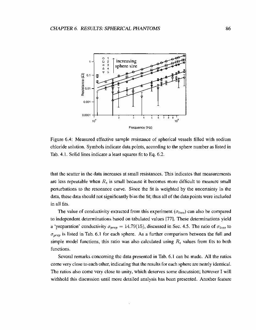
CHAPTER 6. RESULTS: SPHERICAL PHANTOMS
1 o6
Frequency (Hz)
Figure 6.4: Measured effective sample resistance of spherical vessels filled with sodium
chloride solution. Symbols indicate data points, according to the sphere number as listed in
Tab. 4.1. Solid lines indicate a least squares fit to Eq. 6.2.
that the scatter in the data increases at small resistances. This indicates that measurements
are less repeatable when R, is small because it becomes more difficult to measure small
perturbations to the resonance curve. Since the fit is weighted by the uncertainty in the
data, these data should not significantly bias the fit; thus all of the data points were included
in all fits.
The value of conductivity extracted from this experiment (ole,,) can also be compared
to independent determinations based on tabulated values [77]. These determinations yield
a 'preparation' conductivity up,,, = 14.79(15), discussed in Sec. 4.5. The ratio of ole,, to
up,, is listed in Tab. 6.1 for each sphere. As a further comparison between the full and
simple model functions, this ratio was also calculated using Rs values from fits to both
functions.
Several remarks concerning the data presented in Tab. 6.1 can be made. All the ratios
come very close to each other, indicating that the results for each sphere are nearly identical.
The ratios also come very close to unity, which deserves some discussion; however I will
withhold this discussion until more detailed analysis has been presented. Another feature

CHAPTER 6. RESULTS: SPHERICAL PHANTOMS
Sphere Number 40
a increasing sphere size 8
8 E E 8
El @ E
Frequency (kHz)
150 200 250 300 350 400x10~ Frequency (Hz)
Figure 6.5: The sample resistance of spherical phantoms, as a percentage of the resistance
of the transmit coil. The lower plot shows an expanded view of the lower left comer of the
upper plot, showing the region representing the sensitivity limit.

CHAPTER 6. RESULTS: SPHERICAL PHANTOMS
Table 6.1: Ratio of the conductivity, as measured by the ohmic loss experiment, to the
conductivity as determined from preparation of the solutions and comparison to tabulated
values.
sphere number
1
2
clear from Tab. 6.1 is that the uncertainty in the ratio gets larger as the sample volume
decreases, consistent with the larger relative uncertainty in R, seen at these smaller volumes
(Fig. 5.4, Fig. 5.8), as discussed above. Since the uncertainty in R, is reduced when using
the full circuit model, the full circuit model is used to fit all of the resonance curves from
this point forward. This shows that it was beneficial to put the effort into solving the full
circuit model.
Given the good agreement between the separate fits to each data set, all of the data for
sample resistance may be combined together into a global result summarizing the experi-
ment as a whole. The radial dependence can be eliminated from the data if we consider
rearranging Eq. 6.2;
al,,, : a,,,,, simple fit
1.006( 17)
0.988(17)
The quantity on the lefthand side of Eq. 6.3, which we will denote as J, can be calculated
from the data and the experimentally accessible parameters; then the slope of a plot of J as
a function of the square of the frequency should be equal to the conductivity. Additionally,
note that J includes the experimental uncertainties in R,, X, and a. Now we may perform a
linear least squares fit to In J vs In f for the entire data set, with a as the only free parameter.
The value of a obtained from this analysis is al,,, = 14.72(7) Slm. The ratio of al,,, to
a,,,, from the global analysis is al,,, : a,,, = 0.995(11).
A last point about the measurements of losses in spherical samples is that of higher
order terms in the model. The predicted form of the sample resistance, Eq. 3.58, also has
al,,, : a,,,, full fit
1.003(12)
0.997(12)

CHAPTER 6. RESULTS: SPHERICAL PHANTOMS
A 1 term fit
-4 V 2 term fit
I I I I I I I
0.6 0.7 0.8 0.9 1.0 1.1 1.2x10⁶ Frequency (Hz)
Figure 6.6: Residuals of the curve fits to one and two terms of the derived form of the
sample resistance R,. Residuals are shown as a percentage of the measured value of R,.
higher order terms in a/&. Since S involves conductivity and frequency, some deviation
in the frequency dependence of the data from the one-term function R!') is expected. A
suggestion of some curvature is visible in the data set for the largest sphere (Fig. 6.3).
Consider a function now consisting of the first two terms of the series expansion for R,
(Eq. 3.58 or Eq. 6.1)
Note that this equation shows the expected curvature is downwards, in agreement with the
data. Additionally, a still constitutes the only parameter in the equation; both the slope and
curvature are set by a so it is not possible to adjust them both arbitrarily. Using Eq. 6.4,
the size of the second term is predicted to be 7 % that of the first term at 1.25 MHz for
the largest phantom, sphere #I. The data set for this phantom was fit to Eq. 6.4, and the
residuals obtained from this fit are compared to those obtained from the fit to the one-term
function (Eq. 6.2) in Fig. 6.6.
CHAPTER 6. RESULTS: SPHERICAL PHANTOMS 90
Note that the residuals from the one-term fit show only a -- 3 % deviation at 1.25 MHz
rather than the 7 % value predicted from 6.4. Generally the residuals from the two-term fit
appear marginally more consistent with zero than the one-term fit. The resolution of resis-
tance in the experiment is not high enough to state definitively that we are sensitive to the
second term; however the results of this experiment are suggestive that with larger samples
and higher conductivity, the second term may become large enough to make quantitative
comparisons with the model function. What is relevant for the purposes of this thesis is that
there is no clear gain to using the two-term function; fits to one term are sufficient and are
used from this point forward.
6.11 Discussion
The measurements of ohmic losses in spherical phantoms were fit to the predictions of the
spherical model and the resulting conductivity was extracted. The measurement of con-
ductivity from this perturbation technique yields a result that is fully consistent with the
nominal value of conductivity determined from the preparation of the solution (obtained
with the aid of tabulated values of conductivity vs concentration, as measured with other
methods). The implication here is that the eddy current method is actually a very accurate
way to measure absolute electrical conductivity of samples. The method has an inherent
simplicity in that the boundary conditions are well defined. The standard method for mea-
suring the conductivity of solutions involves a conductivity bridge: the solution is placed in
a cell incorporating specialized electrodes. A Wheatstone bridge circuit is then used to ob-
tain the cell impedance by adjusting a resistor in the bridge to balance the currents through
the cell and the resistor [79]. Usually a standardized solution with a well known conduc-
tivity is used to calibrate the apparatus by obtaining the cell constant, because the current
profile is not exactly known. Therefore conventional measurements typically only provide
relative comparisons between conductivities of solutions. Our electrodeless determination
of conductivity requires no calibration with a reference solution and gives an absolute mea-
surement of the conductivity. The current profile inside the sample is completely specified
if the sample is contained in a spherical vessel and immersed in a uniform oscillating mag-
netic field. Therefore this method provides a very clean, straightforward way of measuring
the conductivity of weakly conducting samples.

CHAPTER 6. RESULTS: SPHERICAL PHANTOMS
The fact that al,,, : a,,,, - 1 as measured by the experiment presented in this chapter
deserves more commentary. The results of the spherical model were used to extract al,,,
from the data. The fact that al,,, agrees so well with that predicted using previously reported
measurements of conductivity shows that the spherical model does indeed describe the
losses in samples very well. A final point is that this level of agreement indicates that our
apparatus is understood to a high degree of accuracy.
Measurement of induced magnetic field
Further corroboration of the spherical model was investigated by measuring perturbations
of an oscillating magnetic field as a function of position in the vicinity of a conducting
spherical phantom. The phantom used in this experiment has a 12 cm radius (sphere # 2
according to Tab. 4.1). Measurements of the magnetic field near the sphere were obtained
using the apparatus described in Chapter 4 and analyzed using expressions given in Chap-
ter 5 to extract a measurement of the conductivity a. The z-component of the magnetic field
was measured at five positions along the z-axis; the x-component of the magnetic field was
measured at four positions along the 45" diagonal between z- and x-axes. The unperturbed
field at the centre of the coil was measured when the sphere was not present. For each
placement of the probe coil, the induced field was measured from 0.1 - 1 MHz in 0.1 MHz
increments.
Part of each field component is out-of-phase with the applied field B1 and part is in-
phase. The portions of each field component (z and x) that are out-of-phase and in-phase
were separated by calculating the quantities Dl and P2 as defined by Eqs. 5.51 - 5.52 and
Eqs. 5.61 - 5.62. Since the field perturbation is predominantly out-of-phase, we expect the
term Dl to dominate the response. In fact it was observed that at most, IP21 -- 0.081P1 1, and
hence pl data have a lower relative uncertainty than P2 data. As a result, only fits to the
expression for pl were used to extract conductivity. In a process similar to that followed
for the sample resistance (Eqs. 6.2 - 6.3), we define new functions that involve normalizing
,b' to eliminate the radial dependence
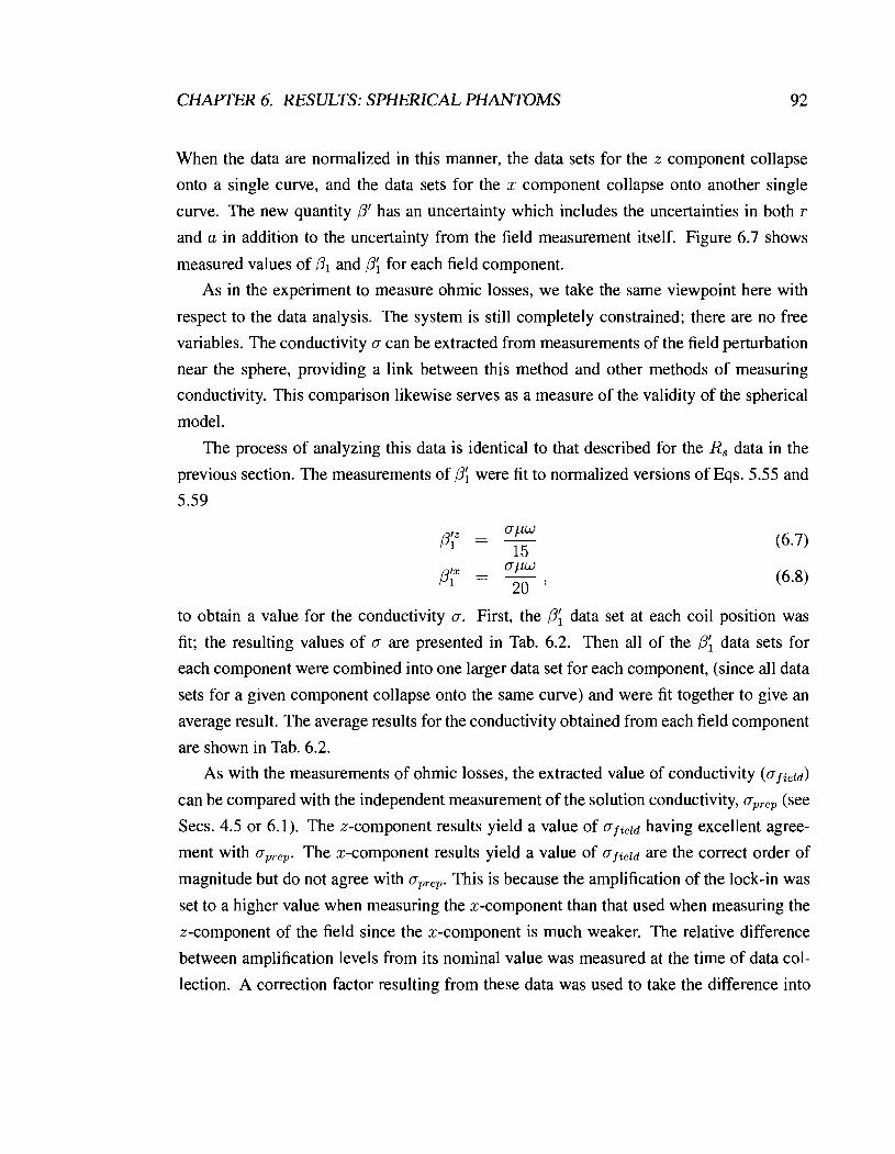
CHAPTER 6. RESULTS: SPHERICAL PHANTOMS 92
When the data are normalized in this manner, the data sets for the z component collapse
onto a single curve, and the data sets for the x component collapse onto another single
curve. The new quantity P' has an uncertainty which includes the uncertainties in both r
and a in addition to the uncertainty from the field measurement itself. Figure 6.7 shows
measured values of Dl and p', for each field component.
As in the experiment to measure ohmic losses, we take the same viewpoint here with
respect to the data analysis. The system is still completely constrained; there are no free
variables. The conductivity a can be extracted from measurements of the field perturbation
near the sphere, providing a link between this method and other methods of measuring
conductivity. This comparison likewise serves as a measure of the validity of the spherical
model.
The process of analyzing this data is identical to that described for the R, data in the
previous section. The measurements of Pi were fit to normalized versions of Eqs. 5.55 and
5.59
PI" = 15
PI" = 20'
to obtain a value for the conductivity a . First, the P; data set at each coil position was
fit; the resulting values of a are presented in Tab. 6.2. Then all of the data sets for
each component were combined into one larger data set for each component, (since all data
sets for a given component collapse onto the same curve) and were fit together to give an
average result. The average results for the conductivity obtained from each field component
are shown in Tab. 6.2.
As with the measurements of ohmic losses, the extracted value of conductivity (ajield)
can be compared with the independent measurement of the solution conductivity, a,,,, (see
Secs. 4.5 or 6.1). The z-component results yield a value of afield having excellent agree-
ment with a,,,,. The x-component results yield a value of afield are the correct order of
magnitude but do not agree with a,,,,. This is because the amplification of the lock-in was
set to a higher value when measuring the x-component than that used when measuring the
z-component of the field since the x-component is much weaker. The relative difference
between amplification levels from its nominal value was measured at the time of data col-
lection. A correction factor resulting from these data was used to take the difference into

CHAPTER 6. RESULTS: SPHERICAL PHANTOMS
l j ~ o l I ll 0
I 0.0 0.2 0.4 0.6 0.8 1.0 Frequency (MHz)
0.06 -
0.05 - 0.04-
0.03 - a- 0.02 - 0.01 -
0.00 -
Figure 6.7: Measurements of the coefficient of the out-of-phase component ( P I ) of the
magnetic field generated by eddy currents in the sphere. Top: The z-component result is
0.0 0.2 0.4 0.6 0.8 1.0 0.0 0.2 0.4 0.6 0.8 1.0 Frequency (MHz) Frequency (MHz)
v r = 14.76 cm v 0 r = 15.66 cm v
r = 16.51 cm v o O o r = 17.11 cm
" O n ' , v o n o
v 0
~ 8 8 ' '
, i " 8
I I 1 I I
shown on the left and the x-component result is shown on the right. Bottom: Normalized
data = r3Pl/a5. Error bars are not shown as they are typically less than the size of the
0.04
0.03-
0.02 - a-
0.01 -
0.00 -
symbols.
v r = 14.59cm 0 r = 15.69 cm v
r=16.69cm v 0 r = 16.79 cm v 0
v 0 • ‹ 8 v o w 'a
v 0 E 9 v 0 a
g 8 ' I
8 I I I I I

CHAPTER 6. RESULTS: SPHERICAL PHANTOMS
z-component results
fit to all data sets:
0.999(11)
x-component results
fit to all data sets:
0.774(8)
corrected for amplification factor:
a = 1.008(11) S/m
Table 6.2: Values of solution conductivities extracted from measurements of each compo-
nent of the magnetic field. The z-component values have been corrected for the background
deviation from the nominal B1 field.
account. When this is done the ratio becomes afield : aPep = 1.008(1 l ) , consistent with
the ratio derived from the z-component field data. While correction for the amplification
was applied in this case, this complication should be avoided in future measurements by
maintaining the same amplification for all measurements where possible.
Measurements of the normalized parameters ,Og and ,OF - representing the portion of
the magnetic field that is in-phase with the applied field - are shown in Figure 6.8. The
values of conductivity obtained from fits to ,Oi were substituted into Eqs. 5.56 and 5.60
and are shown on the same plots as the data for comparison. The agreement of the x-
component data with the prediction is very good. Agreement of the z-component data with
the prediction is good for three of the data sets, albeit with a slight systematic shift.
It is not known why the data set with the largest value of r shows such a large systematic
shift. Measurements of ,O," however are more difficult than ,O; because they require the
detection of a small difference between two large signals, and are thus less likely to be
as accurate as measurements of 0;. For example, at 500 kHz, the voltage on one lock-in
channel was -200 mV when measuring the z-component, and the shift due to the presence
of the sphere was - 10 mV (a 5 % effect); however when measuring the x-component, one
lock-in channel was -100 mV and the shift was -20 mV (a 20 % effect). Therefore the

CHAPTER 6. RESULTS: SPHERICAL PHANTOMS
0.2 0.4 0.6 0.8 1 .O Frequency (MHz)
Figure 6.8: Normalized data of the in-phase coefficient (Pz) of the magnetic field generated
by eddy currents in the sphere. The z-component result is shown on the top graph and the
x-component result is shown on the bottom graph. Theoretical curves are generated from
the value of a calculated from the Pi coefficients. The outlying data set on the top plot is
that taken at the largest radial position along the z-axis.

CHAPTER 6. RESULTS: SPHERTCAL PHANTOMS 96
percent change in the signal due to the presence of the sphere is four times smaller for the
z-component than the x-component.
Additionally, at larger values of r the field map inside the transmit coil becomes less
homogeneous (see Sec. 4.1) making these data more susceptible to systematic errors in
coil placement between measurements. For example, at the probe coil position of 14.76
cm from the isocentre along the z-axis, the field gradient is 5 x 10⁻⁴Blcm-1. However at
the probe coil position of 17.11 cm, the field gradient increases to 1 . 5 ~ 10-~Blcm-'. This
effect is not large enough to explain the largest systematic shift. Considering the level of
agreement between the prediction and all other data sets, this data set is treated as an outlier.
In summary, separating the in-phase component from the out-of-phase component al-
lows calculation of more reliable values of conductivity from the dominant out-of-phase
component. The values of conductivity calculated from the out-of-phase component then
yield excellent predictions for the in-phase component with one exception; thus the mea-
surements of pi are consistent with the measurements of 0;.
6.2.1 Discussion
In this section I presented measurements of the magnetic field generated by eddy currents
induced in a conducting sphere. The electrical conductivity of the sphere was extracted
from the data to serve as an indication of the validity of the measurement technique, as well
as the validity of the spherical model. The conductivity obtained from these experiments
shows complete agreement with independent determinations utilizing tabulated values of
conductivity. While both the loss and field mapping experiments yield excellent results,
the field mapping has several drawbacks since it involves accurate placement of the probe
coil, is generally more complicated to do, and extra work must be done to minimize the
electric field effects. However the value of the experiment is clear because it demonstrates
(i) agreement with the spherical model and (ii) corroboration with the results obtained in
Sec. 6.1. Furthermore, it is again demonstrated that the apparatus that was used is fully
understood. This allows us to move from spherical system having well-defined boundary
conditions to examining induced losses in human subjects.

CHAPTER 6. RESULTS: SPHERICAL PHANTOMS
Summary
In this chapter I presented measurements of the ohmic losses and field perturbation gen-
erated by eddy currents induced in conducting spherical phantoms. The results of each
experiment can be characterized by a value for the electrical conductivity of the phantom.
These extracted values agree with tabulated values for conductivity obtained previously us-
ing other experimental methods. The results of both experiments are consistent with the
spherical model presented in Chapter 3. More importantly, the experiments demonstrate
that the apparatus used is extremely well characterized. Because there are no discrepancies
between the measured properties (losses and magnetic field) and their predicted forms given
by the spherical model, we may conclude that there are no ambiguities in the apparatus and
procedures to collect and analyze these data. Having complete confidence in our apparatus
and methods from these phantom experiments, attention may now be turned to the prob-
lem of measuring ohmic losses in human subjects using this same technique, allowing us
to make statements about the SNR and SAR in very low field MRI experiments. These
experiments are presented in the following chapter.

Chapter 7
Results: Human subjects
In the previous chapter, I presented the results of experiments that were performed to char-
acterize ohmic losses in conducting spherical phantoms over the frequency range 0.01 -
1 MHz. These experiments were repeated to characterize the ohmic losses in human sub-
jects over the same frequency range In this chapter I describe these experiments and present
the results.
Two variations of the experiment were carried out. In the first variation, the receive
coils described in Sec. 4.2 were used to measure the effective sample resistance of human
subjects. A similar set of coils has been used to collect low field HPG lung images [3, 41,
and gives information regarding SNR in low field MRI. In the second variation, which was
designed to extract information relevant to SAR, we used the transmit coil described in
Sec. 4.1 and used in the phantom experiments (Chapter 6).
Each subject was positioned such that the sternum was located in the central xz-plane
of the coil. When using the transmit coil, this ensures that the thorax of the subject occupies
the uniform volume at the centre, as would be the case for MRI of the lungs. Subjects were
positioned as accurately and reproducibly as possible within the coils. The uncertainty in
placement is estimated to be - 1-2 cm. The relative positioning of subjects and coils is
shown in Fig. 7.1 .' I will present and discuss the results of the two experiments separately.
Four male and three female subjects participated in the experiments described in this
'The RMS magnetic field strength inside the coil is N 7 nT and the maximum frequency was 1.25 MHz.
As a comparison, the magnetic field 30 cm from a CRT monitor is N 5 nT at 500 kHz. These experiments
were deemed 'minimal risk' and approved by the SFU Office of Research Ethics.
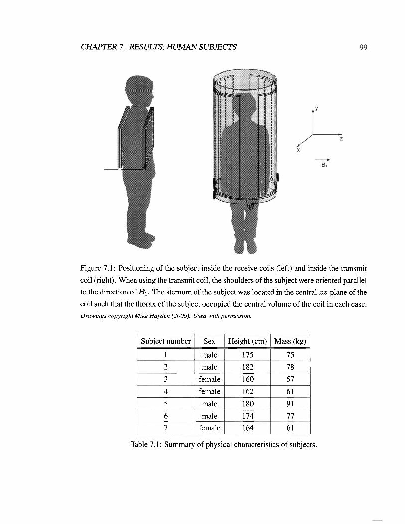
CHAPTER 7. RESULTS: HUMAN SUBJECTS
Figure 7.1: Positioning of the subject inside the receive coils (left) and inside the transmit
coil (right). When using the transmit coil, the shoulders of the subject were oriented parallel
to the direction of B1. The sternum of the subject was located in the central xz-plane of the
coil such that the thorax of the subject occupied the central volume of the coil in each case.
Drawings copyright Mike Hayden (2006). Used with permission.
Subject number
1
2
3
Table 7.1 : Summary of physical characteristics of subjects.
Sex
male
4
5
6
7
male
female
Height (cm)
175
female
male
male
female
Mass (kg)
75
182
160
7 8 -
57
162
180
174
1 64
6 1
9 1
77
6 1
CHAPTER 7. RESULTS: HUMAN SUBJECTS 100
chapter; they ranged in height from 160 - 185 cm, and in mass from 55kg - 9 1 kg. A list
summarizing the physical characteristics of the subjects is provided in Tab. 7.1. Subjects
will be referred to according to the numbers given in the table.
Measurement of SNR
The measurement of R, for human subjects obtained using the receive coils gives the best
indication of the SNR in low field MRI experiments because the filling factor of such a
coil is much higher than that of the transmit coil, and is therefore more sensitive to small
resistances. This increase in sensitivity allows us to probe lower frequencies than is possible
using the transmit coil.
To acquire the data, the subject was positioned between the two receive coils. The coils
were placed 28 cm apart, one in front of and one behind the subject's thorax, as would be the
case for lung imaging. This arrangement is illustrated in Fig. 7.1. The procedure to collect
data was identical to that described for the loss measurement in the previous chapter; the
resonant response of the tuned coil was recorded with and without the subject present inside
the coil, matching the resonance frequency in each case as well as possible. The resonance
curves were fit to the full circuit model function described in Sec. 5.1.2 (Eq. 5.30) to extract
R, in each case.
Data were collected for male subjects #1 and #2. Before commenting on the measured
values of R,, one interesting feature of these experiments is that motion associated with
breathing is apparent in the residuals of fits to the scan, as demonstrated by the example
shown in Fig. 7.2. Since the scans were swept from low frequency to high frequency,
the x-axis can be interpreted as a time axis in this figure. In this particular example the
time to collect the scan was approximately 1 10 seconds. There are approximately - 26
cycles evident in the residuals, indicating an average time of - 4.2 seconds per breath. Not
only are the timescales consistent with a normal respiratory cycle, this effect was observed
directly during the acquisition of this data. When the subject held his breath, the oscillations
stopped, confirming that they are correlated with breathing motions.

CHAPTER 7. RESULTS: HUMAN SUBJECTS
10
- Empty coil - With subject 5
rn - m 3 x 0 rn a, [r
-5
- 1 0 ~ 1 0 ' ~
0.97 0.98 0.99 1.00 1.01 1.02 1.03x10⁶
Frequency (Hz)
Figure 7.2: Residuals from fitting the data collected with the receive coils to the full fit
function. Residuals are expressed as a fraction of the peak value of the data, which has
been normalized to unity.
0 0 0 0
I I I I
0 5 10 15 20 Breath number
Figure 7.3: Normalized amplitudes of the residuals associated with breathing motions. The
peak-to-peak amplitude corresponding to each breath is seen to be related to the slope of
the resonance curve.

CHAPTER 7. RESULTS: HUMAN SUBJECTS
o background 0 foreground
0.2 0.4 0.6 0.8 1.0 1.2x10⁶
Frequency (Hz)
Figure 7.4: The uncertainty in the circuit resistance extracted by the resonance curve fit,
as a percentage of the resistance. The foreground and background are both shown. The
uncertainty in the foreground data is slightly larger than that of the background data, due to
the motions associated with the subject's breathing.
An interesting question is whether the peaks in the residuals correspond to complete
inhalation or exhalation. During inhalation, the lungs expand, increasing the filling factor
and hence decreasing the quality factor. However upon examination of the amplitude of the
oscillations it appears that a shift in the resonant frequency is the important consideration.
Figure 7.3 shows the amplitude of the peak-to-peak residuals (normalized to the largest
value) as a function of breath number. A 180" phase shift is seen at -0.995 MHz, near
the centre of the resonance, hence amplitudes above the resonance frequency are negative.
Since this graph is clearly proportional to the slope of the resonance curve, it is more likely
that the frequency shift gives rise to these residuals rather than the shift in quality factor.
This hypothesis could easily be tested in a future experiment.
Another question that comes to mind when looking at Fig. 7.2 is whether or not the os-
cillations in the foreground data affect the values of the parameters that are extracted from
the curve fit. Figure 7.4 shows the uncertainty in the resistance extracted from the curve fits
of the foreground and background data, as a percentage of the resistance. While the uncer-
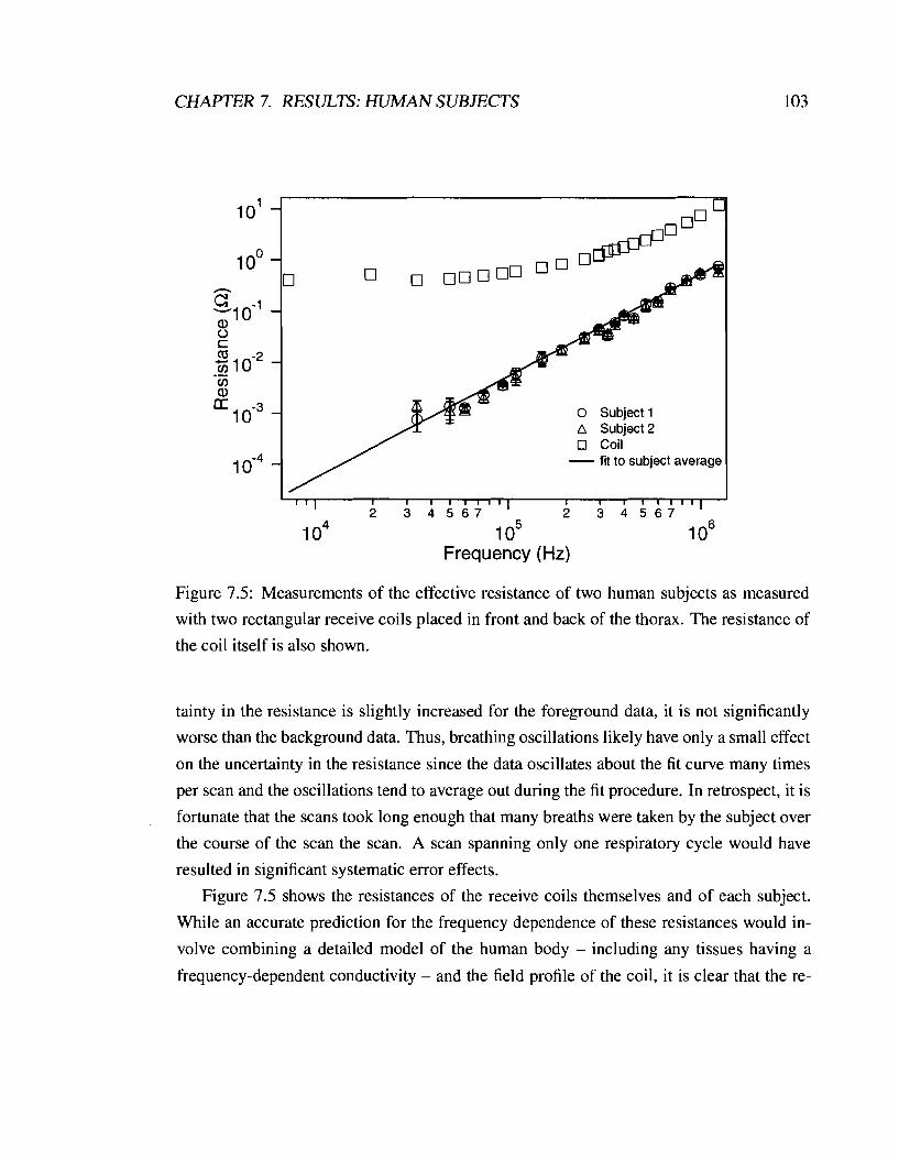
CHAPTER 7. RESULTS: HUMAN SUBJECTS
I I I I I 1 1 1 1 1 1 I I I 1 1 1 1 1 1
2 3 4 5 6 7 2 3 4 5 6 7
1 o4 I o5 1 o6 Frequency (Hz)
Figure 7.5: Measurements of the effective resistance of two human subjects as measured
with two rectangular receive coils placed in front and back of the thorax. The resistance of
the coil itself is also shown.
tainty in the resistance is slightly increased for the foreground data, it is not significantly
worse than the background data. Thus, breathing oscillations likely have only a small effect
on the uncertainty in the resistance since the data oscillates about the fit curve many times
per scan and the oscillations tend to average out during the fit procedure. In retrospect, it is
fortunate that the scans took long enough that many breaths were taken by the subject over
the course of the scan the scan. A scan spanning only one respiratory cycle would have
resulted in significant systematic error effects.
Figure 7.5 shows the resistances of the receive coils themselves and of each subject.
While an accurate prediction for the frequency dependence of these resistances would in-
volve combining a detailed model of the human body - including any tissues having a
frequency-dependent conductivity - and the field profile of the coil, it is clear that the re-

CHAPTER 7. RESULTS: HUMAN SUBJECTS 1 04
sistance of human subjects obeys an f relationship very well, just as was the case for the
sphere. Considering the discussion in Sec. 2.4 that a conductor in the thin limit has an
effective resistance proportional to f 2, this experiment demonstrates that the body appears
to be a weak conductor with a frequency independent conductivity over the two decades of
frequency examined here. The average resistance of the two subjects was fit to a quadratic
relation
R, = k f 2 (7.1)
to demonstrate the f dependence of the resistance. This can be seen in Fig. 7.5 which
shows this fit to the average subject resistance.
The results of this experiment can be compared to those described in Sec. 6.1 -involving
phantom measurements with the transmit coils - in several ways. First of all, we see that
the receive coils are extremely sensitive in comparison to the transmit coil. The minimum
sample resistance that we were able to detect with the transmit coils was -10 ma ; this
value indicates the point at which the uncertainty in the resistance became large and the
scatter also increased in a manner similar to that described in Chapter 6. In contrast, the
receive coil was sensitive to sample resistances of 1 ma . The receive coils were sensitive
down to correspondingly lower frequencies as a result; the transmit coil was sensitive to
samples down to 100 kHz, while the receive coils were sensitive down to 30 kHz.
The measurements obtained for the resistance of the receive coils and the effective sam-
ple resistance of the human body allow an estimate to be made of their contributions to
the noise in the receiver circuit. Recalling the Johnson noise (Eq. 2.21), it is now possible
to estimate the noise due to the receiver coil and body in very low field MRI employing
these coils. The intrinsic SNR could then be estimated from Eq.2.22 if the magnetization is
known.
The primary result of this experiment is that the resistance of the coil dominates the
subject resistance by at least a factor of ten over the entire frequency range studied here. If
we recall that Bidinosti et al. [4] acquired human lung images at 3 mT, corresponding to a
3 ~ e Larmor frequency of 100 kHz, from Fig. 7.5 it can be deduced that R,l : Rbody = 250,
neglecting the resistance of the compensation coils that were used. The Simon Fraser group
magnet can operate up to 10 mT (300 kHz), in which case Rcoil : Rbody x 50. Therefore
the SNR is clearly coil dominated with this receiver; while the SNR is improved by raising
the magnetic field strength (and frequency), careful design of the receiver would allow
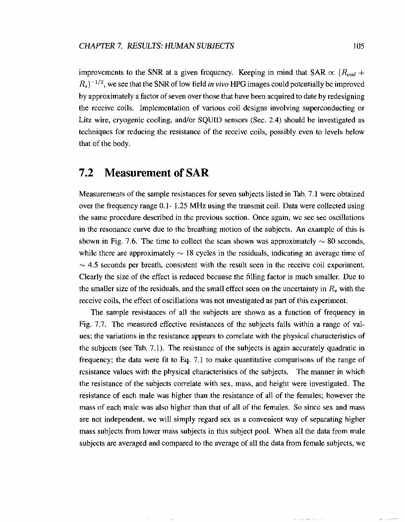
CHAPTER 7. RESULTS: HUMAN SUBJECTS 105
improvements to the SNR at a given frequency. Keeping in mind that SAR m (RCoil + R,)-'I2, we see that the SNR of low field in vivo HPG images could potentially be improved
by approximately a factor of seven over those that have been acquired to date by redesigning
the receive coils. Implementation of various coil designs involving superconducting or
Litz wire, cryogenic cooling, andlor SQUID sensors (Sec. 2.4) should be investigated as
techniques for reducing the resistance of the receive coils, possibly even to levels below
that of the body.
Measurement of SAR
Measurements of the sample resistances for seven subjects listed in Tab. 7.1 were obtained
over the frequency range 0.1 - 1.25 MHz using the transmit coil. Data were collected using
the same procedure described in the previous section. Once again, we see see oscillations
in the resonance curve due to the breathing motion of the subjects. An example of this is
shown in Fig. 7.6. The time to collect the scan shown was approximately - 80 seconds,
while there are approximately - 18 cycles in the residuals, indicating an average time of - 4.5 seconds per breath, consistent with the result seen in the receive coil experiment.
Clearly the size of the effect is reduced because the filling factor is much smaller. Due to
the smaller size of the residuals, and the small effect seen on the uncertainty in R, with the
receive coils, the effect of oscillations was not investigated as part of this experiment.
The sample resistances of all the subjects are shown as a function of frequency in
Fig. 7.7. The measured effective resistances of the subjects falls within a range of val-
ues; the variations in the resistance appears to correlate with the physical characteristics of
the subjects (see Tab. 7.1). The resistance of the subjects is again accurately quadratic in
frequency; the data were fit to Eq. 7.1 to make quantitative comparisons of the range of
resistance values with the physical characteristics of the subjects. The manner in which
the resistance of the subjects correlate with sex, mass, and height were investigated. The
resistance of each male was higher than the resistance of all of the females; however the
mass of each male was also higher than that of all of the females. So since sex and mass
are not independent, we will simply regard sex as a convenient way of separating higher
mass subjects from lower mass subjects in this subject pool. When all the data from male
subjects are averaged and compared to the average of all the data from female subjects, we

CHAPTER 7. RESULTS: HUMAN SUBJECTS
1 Empty coil With subject
Frequency (Hz)
Figure 7.6: Residuals from fitting the data collected with transmit coil to the full fit function.
The oscillations in residuals data are associated with breathing. The influence of breathing
motions is less apparent when using a low filling factor coil such as this one.
clearly see the average male resistance is greater (see Fig. 7.8). The ratio of the coefficient
k is kmale : kfemale = 1.48(5); therefore losses in male subjects were nearly 50% greater
than losses in female subjects, on average. The correlation of the coefficient Ic with mass
and height is illustrated in Fig 7.8. Correlation with both properties is evident, with mass
providing the strongest correlation. A straight line fit of k with the mass was used to cal-
culate the slope, which yields a value of 1.54(6) x 1014RHz-2kg-1. This fit is shown in
Fig. 7.9. The intercept of this straight line fit is nonzero, indicating that a power law fit
might be more appropriate, but there is not enough data to perform a fit that yields a mean-
ingful relation. While the mechanism for variations in resistance is in fact the volume and
number of available eddy current paths, the data are seen to correlate strongly with mass,
which is readily obtained.
The correlation with height is not as strong as that with mass. It is not immediately
obvious if taller subjects should show a larger or smaller resistance than shorter subjects.
Because the sternum of the subject was positioned in the xz-plane of the coil, taller subjects
actually have a smaller fraction of their body inside the coil. However the central homo-
CHAPTER 7. RESULTS: HUMAN SUBJECTS
Figure 7.7: Top: Measurements of the effective resistance of seven human subjects in the
Subject Number 5- 0 1 4 - 0 2 3- a 3
h
C: v 4 - 2- 0 5 a, o a 6 C a D 7 a . 1 - .- a81 0 2 ::
presence of a uniform B1 field. Bottom: Expanded graph showing the higher frequency
data, where error bars have been removed for the sake of clarity. The separation between
subjects is clear. Physical characteristics are listed in Tab. 7.1.
5-
4-
3-
2 -
a Fi
9 8 5
I I I I I I 4 5 6 7 8 9 I
Frequency (Hz) 1 o6

CHAPTER 7. RESULTS: HUMAN SUBJECTS
Frequency (Hz) I o6
Height (cm) , I? 1: 1: 1; 1,:; , *
A Mass scale V Height scale
- z
60 65 70 75 80 85 90
Mass (kg)
Figure 7.8: Top: Plot of the average measured values of effective resistance for males and
females. Bottom: Correlation of the coefficient k with the mass and height of the subjects.

CHAPTER 7. RESULTS: HUMAN SUBJECTS
60 70 80 90 Mass (kg)
Figure 7.9: Top: Mass correlation including straight line fit. Bottom: The graph has been
extended to include the origin.

CHAPTER 7. RESULTS: HUMAN SUBJECTS 110
geneous volume of the coil is always well filled regardless of the height of the subject.
For the time being, the height correlation is not regarded as an important result and more
meaningful correlations are expected to involve mass, volume and body composition.
Deductions may be made about the SAR in the following way. Recalling the time-
averaged power, Eqn. 3.57, and the magnet constant x = B1/I , we can write the time-
average power absorbed by the subject as
since B1 is the peak value of the magnetic field. This becomes
when combined with Eq. 7.1. Finally since the SAR is the power per unit mass of tissue
exposed to the fields, < P > - SAR = ------ - k
- f 2 ~ , 2 . m 2mx2
where m is the total mass exposed to the fields, which are assumed to be uniform.
To derive a conservative estimate of SAR, we use the value of k extracted from the
data set for the largest male, having the highest resistance (subject # 5). Additionally, we
can approximate the filling factor with a simple calculation to arrive at an estimate for the
relevant mass. To make a lower estimate of the mass, the cross-sectional area of subject #
4 - having nearly the lowest mass - was measured as a function of height. The normalized
volume average of the square of the B1 field was estimated to have a value of 76(5) %.
Therefore we use 76 % of the largest subject's mass is involved in the losses giving rise
to the largest subject's. The magnet constant x is known, so all of these values may be
substituted into Eq. 7.4. In this case the coefficient of f2Bf is found to be
To put this value into terms relevant to MRI, we recall the RF pulses discussed in Sec. 2.2.
The angle a between the magnetization vector M and static magnetic field Bo is given by
Eq. 2.7, which may be rewritten as

CHAPTER 7. RESULTS: HUMAN SUBJECTS 11 1
Therefore B1 can be expressed in terms of the duration of a 7r-pulse, which tips M by 180":
Using this relation, the SAR may be calculated as a function of pulse duration and static
field strength so that the result may be compared to the safety guidelines [21,22]. Combin-
ing Eq. 7.4 with Eq. 7.7, we have
Rs SARM 1, t ,
(7.9)
and since the frequency is related to the static field Bo by the Larmor equation 27r f =
yBo, we obtain
Using the measured result for k/2mx2 (Eq. 7.5), we obtain a relation for the SAR as it
depends on the static field strength Bo and the duration of a 7r-pulse
SAR = 1.9 x ~ O - ~ W ~ ~ - ' H Z - ~ T - ~ (t)', This result is the primary conclusion from experiments of losses measured with the
transmit coil. Equation 7.12 is an semi-empirical relation for the SAR during a 7r-pulse,
which we have measured to be valid for uniform fields in the frequency range 0.01 -
1.25 MHz. To demonstrate what it means, some examples are shown in Fig. 7.10. If
we select a field strength Bo, Eq. 7.12 gives SAR as a function of the pulse duration t ,
alone. This function is presented in the case of three static field strengths at which low
field images have been acquired [I, 2,4]. Note that the corresponding Larmor frequencies
used in Refs. [2-4] were probed by this experiment, while our result has been extrapo-
lated up to the Larmor frequency used in Ref. [I]. Also shown in Fig. 7.10 is the USFDA
whole-body SAR exposure guideline, 4 Wkg. From the figure, we can see that very rapid,

CHAPTER 7. RESULTS: HUMAN SUBJECTS
-.-.-.
4 6 8 4 6 8 4 6 8
1 o - ~ 1 1 o - ~ n - pulse duration (ms)
Figure 7.10: Calculation of the SAR in human subjects as it depends on the duration of a
T tipping pulse in milliseconds (which sets the B1 field amplitude) and the strength of the
static field Bo (which sets the Larmor frequency). Values of SAR extracted from our data
are shown for the Bo values used by Refs. [2-41 and an extrapolation of the result up to
the value of Bo used by Ref. [I]. The 4 Wkg level is a maximum whole-body exposure
guideline recommended by the USFDA [2 1 1.
sub-millisecond T-pulses may be applied without exceeding this limit if a sufficiently low
static field strength Bo is employed. For example, at 15 mT a T-pulse lasting 0.02 ms cor-
responds to an SAR of 4 Wkg. However if we extrapolate our relation for low field SAR
(Eq. 7.12) to a Bo value of 1.5 T, we reach an SAR of 4 Wlkg when the T-pulse duration is
1.7 ms. This implies that stronger RF pulses may be applied when using low static fields,
allowing a corresponding reduction in image acquisition time.
Furthermore, note that the result of this experiment shows that a long sequence of many
T-pulses at a very rapid repetition rate (i.e. a high duty cycle) can be safely performed in
very low field MRL This is an important conclusion because T-pulses are avoided in high
field imaging due to the associated SAR. The function of T-pulses is to refocus the trans-
verse magnetization; however an equivalent effect is achieved with a bipolar field gradient.

CHAPTER 7. RESULTS: HUMAN SUBJECTS 113
At the high static field strengths employed in conventional imaging, bipolar gradients are
used to refocus the transverse magnetization, however these gradients are problematic in
very low field imaging where concomitant gradient effects may become important [go].
Therefore we may conjecture that the use of T-pulses may be a safe way to avoid concomi-
tant gradient effects in very low field imaging, and unorthodox pulse sequences employing
more RF pulses may be designed for very low field imaging.
Some care must be taken when drawing conclusions from the whole-body SAR limit.
Since the energy deposition is of course not uniform in a subject, 'hot spots' may form.
Therefore the local maximum SAR is also a consideration, as suggested by [2 11 (Tab. 2.3).
Our measurement of whole-body SAR does not allow conclusions to be drawn regarding
local maxima in SAR.
7.3 Discussion
The work presented in this chapter constitutes the core of this thesis. The main goal was to
obtain an experimental investigation of factors pertaining to SNR and SAR in low field MRI
of human subjects. Experiments probing the SNR show that the simple receive coil design
used by Bidinosti et al. [ 3 , 41 has significantly a higher resistance than that of the human
body. Therefore we conclude that the images they obtained were certainly in the coil-
dominated noise regime. If a focused effort is placed in design of a lower resistance receive
coil for very low field HPG MRI, the advantages of the predicted frequency-independent
SNR in the body-dominated noise regime might yet be reached. Our results imply that an
order of magnitude improvement in SNR could potentially be obtained if the coil resistance
is reduced. Clearly receive coil design will be a crucial consideration for very low field MRI
and must be undertaken if optimum signal-to-noise ratios are to be achieved. Experiments
probing SAR show unequivocally that SAR depends on the square of the frequency of
the applied FW radiation, over the range explored in this experiment. This dependence
was expected from both theoretical predictions based on a spherical model, and from low
frequency extrapolations of high frequency data. The key result of the SAR experiment
is that MRI experiments in which very low static fields are employed offer the possibility
for using stronger oscillating FW fields and hence more complex and more rapid FW pulse
sequences than MRI experiments at high static fields.

CHAPTER 7. RESULTS: HUMAN SUBJECTS 114
One potential benefit of the technique to measure ohmic losses employed in this thesis
is that it may be a sensitive method for measuring SARs in human subjects due to expo-
sure to other sources of electromagnetic fields. Since general exposure guidelines for all
types of electromagnetic exposure exist [81], this method may be useful in conducting SAR
experiments in a much broader context.

Chapter 8
Conclusion
In this thesis I have presented a collection of experiments examining the signal-to-noise
ratio (SNR) and specific absorption rates (SAR) for electromagnetic energy deposition as-
sociated with MRI experiments. The focus was on the very low field regime (- 1 to 100 mT)
relevant to emerging MRI techniques such as those employing hyperpolarized noble gases.
The first set of experiments that were presented involve spherical phantoms; these experi-
ments serve as controls to validate the measurement techniques. Subsequent experiments
involving human subjects yield information regarding fundamental SNR and SAR limits
for real MRI experiments. Ultimately, this information allows design constraints to be es-
tablished for very low field MRI hardware and radiofrequency (RF) pulse sequences. The
experimental results presented in this thesis are believed to be the first of their kind in the
context of very low field MRI.
The first part of this investigation was to perform the control experiments. Uniform
electrically conducting spherical phantoms were exposed to a uniform magnetic field B1 oscillating at frequencies in the range f = 0.1 - 1.25 MHz. The field was generated by
an MRI transmit coil designed for very low field hyperpolarized 3He lung imaging. Mea-
surements of the ohmic losses associated with induced eddy currents in the phantom were
obtained by observing the loading effect caused when the phantom was introduced into the
transmit coil. Five phantoms of varying radii were used in order to examine the size depen-
dence of the losses. Measurements of the spatial variation of magnetic field perturbations
associated with induced eddy currents were obtained for one of these phantoms using a
small probe coil.

CHAPTER 8. CONCLUSION 116
Data from both experiments (ohmic losses and magnetic field perturbations) were fit to
appropriate functions derived from an electrodynamic model of the conducting sphere to
extract a value for electrical conductivity. These values are shown to be in excellent agree-
ment with tabulated reference values. This agreement allows two conclusions to be drawn.
First, because there are absolutely no free parameters in our experiments, we conclude that
the experimental method is valid and that the apparatus is well understood. It also suggests
that a similar level of confidence may be attributed to subsequent measurements involving
human subjects. Second, we infer that the electrodynamic model for a weakly conducting
sphere makes successful predictions over the frequency range of interest.
The next set of experiments in the investigation were those involving human subjects.
As was the case for the spherical phantoms, subjects were exposed to a uniform oscillating
magnetic field, spanning the same frequency range. Two experiments were carried out;
in the first, the field was generated by an MRI receive coil with a design similar to those
used to capture the current state-of-the-art very low field in vivo images of human lung
airspaces [4]. In the second, the field was generated by the same MRI transmit coil as that
used for experiments involving the spherical phantoms. Again, measurements of the ohmic
losses associated with induced eddy currents in the subjects were obtained by observing the
loading effect on the appropriate coil.
The first experiment involving human subjects provides information regarding the SNR
in very low field MRI experiments that is essential in order to improve image quality. The
measurement allows a direct comparison of the noise generated by a human subject to the
intrinsic noise in the coil at low frequencies. These measurements show that the subject is
not the limiting source of Johnson noise for the particular receive coil used here. Specifi-
cally, the noise contribution from the coils dominates that of the subject by at least a factor
of ten in the frequency range that was explored. Therefore our measurements demonstrate
that approximately a factor of ten improvement to the SNR may be obtained by pursuing de-
signs for lower resistance receive coils or alternate detection methods. The clear dominance
of the coil resistance indicates that the implementation of cryogenic, Litz or superconduct-
ing wire, and other coil designs will be crucial to the success of low field imaging.
The second experiment yields a direct measurement indicative of the SAR under realis-
tic imaging conditions. This in turn provides design constraints on RF pulse sequences. We
deduce a whole-body average SAR of 1.9(3) x f 2B; Wkg (MKS units), using con-
CHAPTER 8. CONCLUSION 117
servative estimates. By expressing the magnetic field strength B1 in terms of the duration of
an RF pulse that tips spins by 1 80•‹, we show that continuous application of sub-millisecond
T-pulses (which would normally be unsafe under high field imaging conditions) does not
exceed recommended whole-body SAR levels at sufficiently low static field strengths. This
result leads us to the first of two principal conclusions of this thesis: that innovative and
complex new pulse sequences involving many strong and rapid RF pulses may be safely
applied for use in very low field HPG imaging.
Suggestions for technical and methodological improvements to the experiments pre-
sented in this thesis include the following. A more thorough field mapping experiment
could be done; measurements could be taken at larger number of positions, including points
out of the xz-plane, measurements of the y-component of the field, and possibly measure-
ments employing a pair of probe coils, to take advantage of the symmetry of the induced
magnetic fields. A calibrated system could be developed to more accurately position the
probe coil. Furthermore, the use of network analyzers is common in cavity perturbation
experiments, for example those involving microwave resonators. A network analyzer could
be used in place of the lock-in to potentially simplify the experiment.
Experiments could also be done using other transmit coils. Based on our observation
of electric field effects, it would be worth pursuing a new design of transmit coil, that has
interleaved windings to balance electric potentials inside the coil. Also, experiments em-
ploying the actively shielded design recently developed for use as a very low field MRI
transmit coil [73,75] could be performed. This coil would also be less sensitive to its envi-
ronment and require less space to conduct the experiments. It is suspected that combination
of interleaved windings and active shielding would be a very robust transmit coil design.
Numerous experiments related to the work presented in this thesis are of scientific in-
terest. First, there are many parameters that could be varied in the study of spherical phan-
toms. The conductivity and radius of the phantoms could be varied such that the second
term of the series expansion of the sample resistance becomes more apparent. Materi-
als having a frequency-dependent conductivity would certainly be interesting to study and
would provide a comparison with physiologically relevant systems. Second, other shapes
of phantoms might be explored. While mathematically more complicated, approximations
do exist for shapes such as a hemisphere [82] and a cylinder [65, 831. Hemispheres have
been examined in the high frequency limit [82] while experiments involving cylinders have

CHAPTER 8. CONCLUSlON 118
been examined in the low frequency limit [84]; corroboration of these results would be a
worthwhile exercise.
A large number of further experiments involving human subjects could be performed.
A few examples include the following. Measurements could be collected involving many
different subjects having a range of physical characteristics (such as mass and body type)
to investigate in more detail the relation between these properties and the observed loading
effect on the coil. The oscillations associated with the subject's breathing that were evident
could also be studied in more detail. Interesting topics include the study of the possible
phase shift at resonance, qualitative correlation of the oscillations in the data with exhalation
and inhalation, and quantitative determination of the changes to both the quality factor and
resonance frequency associated with breathing motions.
The second principal conclusion of this thesis is that a focused effort should be devoted
to the design of specialized receive coils for very low field MRI. It is certainly possible to
reduce the radiation resistance of receive coils with an appropriate arrangement of multiple
coils. However a greater reduction of the resistance is anticipated for designs utilizing
superconducting or Litz wire and/or cryogenically cooled coils. In order to compare the
performance of such coils to that of resistive, room temperature coils, experiments must be
carefully designed to take into consideration the complicated dependence of the SNR on the
shape, size, temperature and conductivity of the coil. Another route to develop a high SNR
receiver is to investigate novel new sensors such as those incorporating SQUIDS. Since a
properly designed high SNR receiver is essential for the acquisition of high quality images
and will have a significant impact on very low field MRI in years to come, these studies
should begin immediately.
Finally, the methods employed in this thesis to measure ohmic losses in conducting
bodies might be applied to other fields. It has been demonstrated that this method provides
a sensitive, absolute measurement of solution conductivities, with an inherent simplicity
that arises because of extremely well-defined boundary conditions and geometric factors
that are lacking in standard approaches. In addition, the apparatus provides information
regarding specific absorption rates that in principle could be applicable to a broad range of
other fields. In particular, this method may be useful in evaluating the physiological effects
associated with very low frequency electromagnetic radiation.
Bibliography
[ l ] E. Durand, G. Guillot, L. Darrasse, G. Tastevin, P.J. Nacher, A. Vignaud, D. Vattolo,
and J. Bittoun. CPMG measurements and ultrafast imaging in human lungs with
hyperpolarized helium-3 at low field (0. I T). Magn. Reson. Med., 47:75-8 I , 2002.
[2] A.K. Venkatesh, A.X. Zhang, J. Mansour, L. Kubatina, C.H. Oh, G. Blasche, M.S.
~ n l i i , D. Balamore, F.A. Jolesz, B.B. Goldber, and M.S. Albert. MRI of the lung
gas-space at very low-field using hyperpolarized noble gases. Magn. Reson. Imag.,
21 1773-776, 2003.
[3] C.P. Bidinosti, J. Choukeife, P.J. Nacher, and G. Tastevin. In vivo NMR of hyper-
polarized 3He in the human lung at very low magnetic fields. J. Magn. Reson., 162:
122-132,2003.
[4] C.P. Bidinosti, J. Choukeife, G. Tastevin, P.J. Nacher, and A Vignaud. MRI of the
lung using hyperpolarized 3He at very low magnetic field (3 mT). MAGMA, 16(6):
255-258.2004.
[5] R.W. Mair, M.I. Hrovat, S. Patz, M.S. Rosen, I.C. Ruset, G.P. Topulos, L.L. Tsai,
J.P. Butler, F.W. Hersman, and R.L. Walsworth. 3He lung imaging in an open access,
very-low-field human magnetic resonance imaging system. Magn. Reson. Med., 53:
745-749,2005.
[6] A.N. Matlachov, P.L. Volegov, M.A. Espy, J.S. George, and R.H. Kraus Jr. SQUID
detected NMR in microtesla magnetic fields. J. Magn. Reson., 170: 1-7,2004.
[7] R. McDermott, S. Lee, B. ten Haken, A.H. Trabesinger, A. Pines, and J. Clarke. Mi-

BIBLIOGRAPHY 120
crotesla MRI with a superconducting quantum interference device. PNAS, 101 :7857-
786 1,2004.
[8] M. MoBle, W.R. Myers, S.-K. Lee, N. Kelso, M. Hatridge, A. Pines, and J. Clarke.
Squid-detected in vivo rnri at microtesla magnetic fields. IEEE Transactions on Ap-
plied Superconductivity, 15(2):757 - 60,2005.
[9] S.K. Lee, M. MoBle, W. Myers, N. Kelso, A.H. Trabesinger, A. Pines, and J. Clarke.
SQUID-detected MRI at 132 pT with TI-weighted contrast established at 10 pT -
300 mT. Magn. Reson. Med., 53:9-14,2005.
[lo] D.I. Hoult and R.E. Richards. The signal-to-noise ratio of the nuclear magnetic reso-
nance experiment. J. Magn. Reson., 24(1):7 1 - 85, 1976.
[l 11 D.I. Hoult and P.C. Lauterbur. The sensitivity of the zeugmatographic experiment. J.
Magn. Reson., 34:425433, 1979.
[I 21 D.G. Gadian. Radiofrequency losses in NMR experiments on electrically conducting
samples. J. Magn. Reson., 34:449455, 1979.
[13] O.P. Gandhi and X.B. Chen. Specific absorption rates and induced current densities
for an anatomy-based model of the human for exposure to time-varying magnetic
fields of MRI. Magn. Reson. Med., 41 (4):8 16-823, 1999.
[14] C.M. Collins, S. Li, and M.B. Smith. SAR and B1 field distributions in a heteroge-
neous human head model within a birdcage coil. Magn. Reson. Med., 40:847-856,
1998.
[15] F.G. Shellock. Radiofrequency energy-induced heating during MR procedures: A
review. J. Magn. Reson. Imaging, 2000.
[16] W. Liu, C.M. Collins, and M.B. Smith. Calculations of B1 distribution, specific energy
absorption rate, and intrinsic signal-to-noise ratio for a body-size birdcage coil loaded
with different human subjects at 64 and 128 MHz. Appl. Magn. Reson., 295 - 18,
2005.

BIBLIOGRAPHY 121
[I71 P. Styles, N.F. Stoffe, C.A. Scott, D.A. Cragg, F. Row, D.J. White, and P.C.J. White. A
high-resolutions NMR probe in which the coil and preamplifier are cooled with liquid
helium. J. Magn. Reson., 60:397-404, 1984.
[18] L. Darrasse and J.-C. Ginefri. Perspectives with cryogenic RF probes in biomedical
MRI. Biochimie, 85:9 l5-937,2OO3.
[19] A.R. Cross, M. McDonald, J. Parra Robles, and G.E. Santyr. Laser-polarized 12'Xe
NMR at 1.88 T and 8.5 mT: a signal-to-noise ratio comparison. J. Magn. Reson., 162:
24 l-249,2003.
[20] J. Parra-Robles, A.R. Cross, and G.E. Santyr. Theoretical signal-to-noise ratio and
spatial resolution dependence on the magnetic field strength for hyperpolarized noble
gas magnetic resonance imaging of human lungs. Med. Phys., 32:221-229,2005.
[21] U.S. Department of Health, Food Human Services, and Drug Administration Office
of Device Evaluation. Criteria for significant risk investigations of magnetic resonance
diagnostic devices. http:Nwww.fda.govlcdrh/odelguidancel793.pdf, 2003. FOD #793.
[22] Health Canada. Guidelines on exposure to electromagnetic fields from mag-
netic resonance clinical systems - Safety Code 26. http:Nwww.hc-sc.gc.ca/ewh-
semt/pubslradiationl87ehd-dhm127/index~e.html,2004.
[23] G. Sergiadis, J. Sakellaris, and E.E. Kriezis. Electromagnetic field distribution and
developed losses inside a finite cylinder and sphere under MRI conditions. IEEE
Trans. Med. Imaging, 7(4):381 - 5, 1988.
[24] L.S. Petropoulos and E.M. Haacke. Higher-order frequency-dependence of radiofre-
quency penetration in planar, cylindrical, and spherical-models. J. Magn. Reson., 9 1
(3):466-474, 1 99 1.
[25] M.D. Harpen. Influence of skin depth on NMR coil impedance. part ii. Phys. Med.
Biol., 33(5):597405, 1988.
[26] R.A. Waldron. The theory of waveguides and cavities. Gordon and Breach, New York,
1967.

BIBLIOGRAPHY 122
[27] F. Bloch, W.W. Hansen, and M. Packard. Nuclear induction. Phys. Rev., 2 1 : 127, 1946.
[28] E.M. Purcell, R.V. Pound, and N. Bloemergen. Nuclear magnetic resonance absorp-
tion in hydrogen gas. Phys. Rev., 78:986-987, 1946.
[29] F. Reif. Fundamentals of statistical and thermal physics. McGraw-Hill, Inc., 1965.
[30] A. Abragam. The Principles of Nuclear Magnetism. Oxford University Press Inc.,
1961.
[3 11 C.P. Slichter. Principles of magnetic resonance. Springer-Verlag, Berlin ; New York,
2nd edition, 1978.
[32] P.C. Lauterbur. Image formation by induced local interactions: examples employing
nuclear magnetic resonance. Nature, 242: 190-1 9 1, 1973.
[33] P. Mansfield and P.K. Grannell. NMR 'diffraction' in solids? Journal of Physics C
(Solid State Physics), 6(22):422 - 6, 1 973.
[34] P. T. Callaghan. Principles of Nuclear Magnetic Resonance Microscopy. Oxford
University Press, Oxford, 199 1.
[35] M.A. Brown and R.C. Semelka. MRI: Basic principles and applications. Wiley, New
York, 1995.
[36] M. Estilaei, A. MacKay, K. Whittall, and J. Mayo. In vitro measurements of water
content and T2 relaxation times in lung using a clinical MRI scanner. J. Magn. Reson.
Imaging, 9(5):699-703, 1999.
[37] V.M. Mai, J. Knight-Scott, and S. S. Ben: Improved visualization of the human lung
in 'H MRI using multiple inversion recovery for simultaneous suppression of signal
contributions from fat and muscle. Magn. Reson. Med., 4 1 :866-870, 1999.
[38] H.U. Kauczor and K.F. Kreitner. Contrast-enhanced MRI of the lung. Eur: J. Radiol-
ogy, 34(3): 196-2O7,2OOO.
[39] F.D. Colegrove, L.D. Schearer, and GK Walters. Polarization of 3He gas by optical
pumping. Phys. Rev., l32:256 1-2572, 1963.

BIBLIOGRAPHY 123
[40] M.A. Bouchiat, T.R. Carver, and C.M. Varnum. Nuclear polarization in He3 gas in-
duced by optical pumping and dipolar exchange. Phys. Rev. Lett., 5:373-375, 1960.
[4 11 W. Happer. Optical pumping. Rev. Mod. Phys., 44: 169-249, 1972.
[42] T. Chupp and S. Swanson. Medical imaging with laser polarized noble gases. Adv.
Atm. Mol. Opt. Phys, 454 1, 200 1.
[43] M. Salerno, T.A. Altes, J.P. Mugler 111, M. Nakatsu, H. Hatabu, and E.E. de Lange.
Hyperpolarized noble gas MR imaging of the lung: Potential clinical applications.
Eur: J. Radiology, 40(1):3344,2001.
[44] H.E. Moller, X.J. Chen, B. Saam, K.D. Hagspiel, G.A. Johnson, T.A. Altes, E.E.
de Lange, and H.U. Kauczor. MRI of the lungs using hyperpolarized noble gases.
Magn. Reson. Med., 47: 1029-105 1,2002.
[45] M.S. Albert, G.D. Cates, B. Driehuys, W. Happer, B. Saam, C.S. Springer Jr, and
A. Wishnia. Biological magnetic resonance imaging using laser-polarized 12'Xe. Na-
ture, 370: 199-201, 1994.
[46] H. Middleton, R.D. Black, and B. Saam. MR imaging with hyperpolarized He-3 gas.
Magn. Reson. Med., 33:27 1-275, 1995.
[47] R.D. Black, H.L. Middleton, and G.D Cates. In vivo He-3 MR images of guinea pig
lungs. Radiology, 19993674370, 1996.
[48] L.D. Landau, E.M. Lifshitz, and L.P. Pitaevskii. Electrodynamics of continuous me-
dia. Pergamon Press, 2nd edition, 1984.
[49] W.A. Edelstein, G.H. Glover, C.J. Hardy, and R.W. Redington. The intrinsic signal-
to-noise ratio in NMR imaging. Magn. Reson. Med., 3:604-6 18, 1986.
[50] A.S. Hall, N. Alford, T.W. Button, D.J. Gilderdale, K.A. Gehrig, and I.R. Young. Use
of high temperature superconductor in a receiver coil for magnetic resonance imaging.
Magn. Reson. Med., 20:340-343, 199 1.
BIBLIOGRAPHY
[51] A.S. Hall, B. Barnard, P. McArthur, D.J. Gilderdale, I.R. Young, and G.M. Bydder.
Investigation of a whole-body receiver coil operating at liquid nitrogen temperatures.
Magn. Reson. in Med., 7(2):230-235, 1988.
[52] T. Claasen-Vujcic, H.M. Borsboom, H.J.G. Gaykema, and T. Mehlkopf. Transverse
low-field RF coils in MRI. Magn. Reson. Med. (USA), 36(1): 1 11- 16, 1996.
[53] F.D. Doty, G. Entzminger Jr, and C.D. Hauck. Error-tolerant RF litz coils for
NMRIMRI. J. Magn. Reson., 140(1): 17-3 1, 1999.
[54] F. Resmer, H. Seton, and J.M.S. Hutchison. Cryogenic Litz-wire receiver for low field
MRI. Proc. Intl. Soc. Mag. Reson. Med., 1 l(156 1 ), 2004.
[55] C. Gabriel, S. Gabriel, and E. Corthout. The dielectric properties of biological tis-
sues: 11. Measurements in the frequency range 10 Hz to 20 GHz. Phys. Med. Biol.,
4 1 :225 1-2269, 1996.
[56] J. Van Bladel. Electromagnetic Fields. McGraw-Hill Book Company, New York,
1964.
[57] W.R. Smythe. Static and Dynamic Electricity. McGraw-Hill Book Company, Toronto,
3'd edition, 1968.
[58] E.E. Kriezis, T.D. Tsiboukis, S.M. Panas, and J.A. Tegopoulos. Eddy currents: theory
and applications. Proceedings of the IEEE, 80(10):1559 - 89, 1992.
[59] A.G. Nekut and B.R. Spies. Petroleum exploration using controlled-source electro-
magnetic methods. Proceedings of the IEEE, 77(2):338 - 62, 1989.
[60] R. Rabinovici and T.J.E. Miller. Eddy-current losses of surface-mounted permanent-
magnet motors. IEE Proceedings-Electric Power Applications, 144(1):61 - 4, 1997.
[61] J.R. Wait. A conducting sphere in a time varying magnetic field. Geophysics, 16:666
-672, 1951.
[62] S.H. Ward. Unique determination of conductivity, susceptibility, size, and depth in
mulifrequency electromagnetic exploriation. Geophysics, 2453 1 - 546, 1959.

BIBLIOGRAPHY 125
[63] J.W. Luquire, W.E. Deeds, and C.V. Dodd. Axially symmetric eddy currents in a
spherical conductor. J. App. Phys., 4 1 :3976-82, 1970.
[64] C.V. Dodd and W.E. Deeds. Analytical solutions to eddy-current probe-coil problems.
J. App. Phys., 39(6):2829-2838, 1968.
[65] J.A. Tegopoulos and E.E. Kriezis. Eddy currents in linear conducting media. Elsevier,
1984.
[66] J.W. Carlson. Radiofrequency field propagation in conducting NMR samples. J.
Magn. Reson., 78563, 1988.
[67] E.M. Chapple, C.P. Bidinosti, and M.E. Hayden. RF power deposition in the thin
limit: The sphere in a uniform RF field revisited in the context of very low field MRI.
In preparation, 2006.
[68] J.D. Jackson. Classical Electrodynamics. John Wiley & Sons, Inc., 3rd edition, 1999.
[69] M.D. Harpen. Influence of skin depth on NMR coil impedance. Phys. Med. Biol., 33
(3):329-337, 1988.
[70] F. London. Superjuids - Macroscopic theory of Superconductivity, volume 1. Dover
Publications, 196 1.
[7 11 D.J. Griffiths. Introduction to Electrodynamics. Prentice Hall Upper Saddle River,
New Jersey, 1999.
[72] M. Abramowitz and LA. Stegun. Handbook of Mathematical Functions. Dover, New
York, 1970. 9th printing. Section 10.1, p. 437.
[73] C.P. Bidinosti, I.S. Kravchuk, and M.E. Hayden. Active shielding of cylindrical
saddle-shaped coils: Application to wire-wound RF coils for very low field NMR
and MRI. J. Magn. Reson., 177:3 143,2005.
[74] C.E. Hayes, W.A. Edelstein, and J.F. Schneck. Magnetic Resonance Imaging, chapter
Radio frequency resonators. W.B. Saunders, Philadelphia, 1 988.

BIBLIOGRAPHY 126
[75] I.S. Kravchuk. Active shielding of cylindrical transmit coils for low-field magnetic
resonance imaging. Master's thesis, Simon Fraser University, August 2005.
[76] C.P. Bidinosti, I.S. Kravchuk, J. Cha, N.A. David, and M.E. Hayden. Wire-wound B1
coils for low frequency MRI. Proc. Intl. Soc. Mag. Reson. Med., 1 1 : 155 1, 2004.
[77] Editor R.C Weast. CRC Handbook of Chemistry and Physics. CRC Press, Inc, 59th
edition, 1979. p D-299 - D-300.
[78] R.E. Collin and F.J. Zucker. Antenna Theory, part I. McGraw-Hill Inc., Toronto,
1969. p. 36.
[79] L.M. Raff. Principles of Physical Chemistry. Prentice-Hall, Upper Saddle River, NJ,
2001.
[SO] J.L. Hobson. Concomitant gradients in low-field NMR studies of restricted diffusion.
Master's thesis, Simon Fraser University, 2006.
[81] Health Canada. Limits of human exposure to radiofrequency electromagnetic fields
in the frequency range from 3kHz to 300 GHz - Safety Code 6. http://www.hc-
sc.gc.ca/ewh-semt/pubs/radiation/99ehd-dhm237/indexe.html, 2004.
[82] M. D. Harpen. Eddy current disruption: Effect on nuclear magnetic resonance coil
impedance and power loss. Medical Physics, l6(5):781-784, 1989.
[83] D.X. Guan and J.W. Huo. Electromagnetic-field distribution and developed losses
inside a finite cylinder and sphere under MRI conditions - comment. IEEE Trans.
Med. lmag., pages 229-230, 1 99 1.
[84] E.M. Chapple. Towards hyperpolarized gas imaging in ultra-low magnetic fields:
signal to noise considerations, August 2003. Undergraduate Honours Thesis.