Functional Optimization- and Integro-PartialDifferential Equations-Based Mathematical Modeling

and Numerical Simulation

Applications to Heat Transfer, Crack Propagation,and Shape Design

C u m u l a t i v e H a b i l i t a t i o n T h e s i s

in the Field of Mathematics

submitted to the

Faculty of Mathematics, Computer Science, and Statistics

of the Ludwig-Maximilians University Munich

by

Dr. Peter Philip,

born on December 15, 1971 in Hillerød, Denmark

Referees:

1. Prof. Dr. L. Erdös

2. Prof. Dr. F. Bornemann

3. Prof. Dr. H. Garcke

Date of colloquium (defense): October 29, 2012

Functional Optimization- and Integro-PartialDifferential Equations-Based Mathematical Modeling

and Numerical Simulation

Applications to Heat Transfer, Crack Propagation,and Shape Design

Peter Philip

March 28, 2012

i

Preface

This thesis consists of the following nine selected refereed articles [1, 2, 3, 4, 5, 6, 7, 8, 9],previously published in the period 2005–2012, preceded by an Introduction.

The following list provides the bibliographic information for the mentioned papers inthe order they are included in the thesis. The actual papers can be found after thesections containing the Introduction and further relevant references.

Except [6, 7], all included articles constitute collaborations. I have contributed originalnumerical code for the included papers [1, 2, 4, 5, 7, 9]. In particular, I have beenthe initial principal developer of the numerical simulation software WIAS-HiTNIHS(cf. Sec. 1.1.5 of Introduction). In my judgment, all coauthors have contributed aboutequal shares to the joint papers [1, 2, 3, 4, 8]. My main contribution to [9] is [9, Sec. 3].

Bibliography of Included Papers

[1] C. Meyer and P. Philip. Optimizing the temperature profile during sublima-tion growth of SiC single crystals: Control of heating power, frequency, and coilposition. Crystal Growth & Design 5 (2005), 1145–1156.

[2] J. Geiser, O. Klein, and P. Philip. Influence of anisotropic thermal con-ductivity in the apparatus insulation for sublimation growth of SiC: Numericalinvestigation of heat transfer. Crystal Growth & Design 6 (2006), 2021–2028.

[3] C. Meyer, P. Philip, and F. Tröltzsch. Optimal Control of a SemilinearPDE with Nonlocal Radiation Interface Conditions. SIAM J. Control Optim. 45(2006), 699–721.

[4] J. Geiser, O. Klein, and P. Philip. A finite volume scheme designed foranisotropic heat transfer in general polyhedral domains. Advances in Mathemati-cal Sciences and Applications (AMSA) 18 (2008), 43–67.

[5] O. Klein, Ch. Lechner, P.-É. Druet, P. Philip, J. Sprekels, Ch. Frank-Rotsch, F.-M. Kießling, W. Miller, U. Rehse, and P. Rudolph. Nu-merical simulations of the influence of a traveling magnetic field, generated by aninternal heater-magnet module, on liquid encapsulated Czochralski crystal growth.Magnetohydrodynamics 45 (2009), 257–267, Special Issue: Selected papers ofthe International Scientific Colloquium Modelling for Electromagnetic Process-ing, Hannover, Germany, October 27-29, 2008.

ii

[6] P. Philip. A Quasistatic Crack Propagation Model Allowing for Cohesive Forcesand Crack Reversibility. Interaction and Multiscale Mechanics: an InternationalJournal (IMMIJ) 2 (2009), 31–44.

[7] P. Philip. Analysis, Optimal Control, and Simulation of Conductive-RadiativeHeat Transfer. Mathematics and its Applications / Annals of AOSR 2 (2010),171–204.

[8] P.-É. Druet and P. Philip. Noncompactness of integral operators modelingdiffuse-gray radiation in polyhedral and transient settings. Integral Equations andOperator Theory (IEOT) 69 (2011), 101–111.

[9] P. Philip and D. Tiba. Shape Optimization via Control of a Shape Functionon a Fixed Domain: Theory and Numerical Results, pp. 285–299 in NumericalMethods for Differential Equations, Optimization, and Technological Problems:Celebration proceedings dedicated to Prof. Pekka Neittaanmaki’s 60th birthday.Springer, 2012, in press.

1

Contents

Preface i

Bibliography of Included Papers i

1 Introduction 1

1.1 Conductive-Radiative Heat Transfer . . . . . . . . . . . . . . . . . . . . 1

1.1.1 Model Equations . . . . . . . . . . . . . . . . . . . . . . . . . . 1

1.1.2 Optimal Control of Heat Sources . . . . . . . . . . . . . . . . . 4

1.1.3 Induction Heating: Model and Control . . . . . . . . . . . . . . 7

1.1.4 Anisotropic Thermal Conductivity . . . . . . . . . . . . . . . . 10

1.1.5 Numerical Simulation Software WIAS-HiTNIHS . . . . . . . . . 15

1.2 Crack Propagation . . . . . . . . . . . . . . . . . . . . . . . . . . . . . 16

1.3 Shape Design . . . . . . . . . . . . . . . . . . . . . . . . . . . . . . . . 20

References 26

Included Previously Published Papers 30

1 Introduction

1.1 Conductive-Radiative Heat Transfer

1.1.1 Model Equations

Except for [6, 9], the included papers are all in some way related to the topic of mathe-matical modeling of conductive-radiative heat transfer, with special focus on numericalsimulation and control. The need for modeling, simulation, and control of conductive-radiative heat transfer arises from industrial applications such as single crystal growthfrom vapor or melt (see references in the included papers, in particular in [1, 5, 7]).

Transient conductive heat transfer is modeled by

∂ε(x, θ)

∂t− div

(κ(x, θ)∇ θ

)= f(t, x) in ]0, T [×Ω, (1)

2

where T > 0 represents the final time, θ(x, t) represents absolute temperature dependingon the space variable x and the time variable t, ε > 0 represents internal energy, κ > 0represents thermal conductivity, and f models heat sources or sinks. The stationaryvariant of (1), where the term ∂ε(x,θ)

∂tis missing and θ, f do not depend on t, namely

− div(κ(x, θ)∇ θ

)= f(x) in Ω, (2)

is also of interest and is considered as well. The space domain Ω ⊆ R3 is assumed toconsist of two parts Ωs and Ωg, where Ωs represents an opaque solid and Ωg representsa transparent gas:

Ω = Ωs ∪ Ωg, Ωs ∩ Ωg = ∅, Σ := Ωs ∩ Ωg. (3)

This decomposition of Ω is to facilitate the modeling of radiative heat transfer, wherenonlocal radiative heat transport is considered between points on the surface Σ of Ωg.The open sets Ω, Ωs, Ωg need to satisfy a number of geometrical regularity assumptions,see, e.g., [7, Sec. 2.1], which also has illustrating figures.Continuity of the normal component of the heat flux on the interface Σ between solidand gas, where one needs to account for radiosity R and for irradiation J , yields thefollowing interface condition for (2) (the same works for (1) after replacing the spacedomains by the corresponding time-space cylinders):(

κ(x, θ)∇ θ)Ωg

·ng +R(θ)− J(θ) =(κ(x, θ)∇ θ

)Ωs

·ng on Σ. (4)

Here, ng denotes the unit normal vector pointing from gas to solid and denotes re-striction (or trace). Thus, effectively, (2) consists of two equations, one on Ωs and oneon Ωg, coupled via (4) (and analogously for (1)).In the context of diffuse-gray radiation, where reflection and emittance are taken to beindependent of the angle of incidence and independent of the wavelength, R is modeledvia the well-known radiosity equation(

Id−(1− ε)K)(R) = εσ|θ|3θ, (5)

where Id denotes the identity operator, σ ∈ R+ represents the Boltzmann radiationconstant, ε = ε(x, θ) ∈ [0, 1] represents the emissivity of the solid surface, and Kdenotes the nonlocal integral radiation operator defined by

K(ρ)(x) :=

∫Σ

V (x, y)ω(x, y) ρ(y) dy for a.e. x ∈ Σ, (6)

ω(x, y) :=

(ns(y) · (x− y)

) (ns(x) · (y − x)

)π((y − x) · (y − x)

)2 for a.e. (x, y) ∈ Σ× Σ, (7)

V (x, y) :=

0 if Σ∩ ]x, y[6= ∅,1 if Σ∩ ]x, y[= ∅

for each (x, y) ∈ Σ× Σ, (8)

3

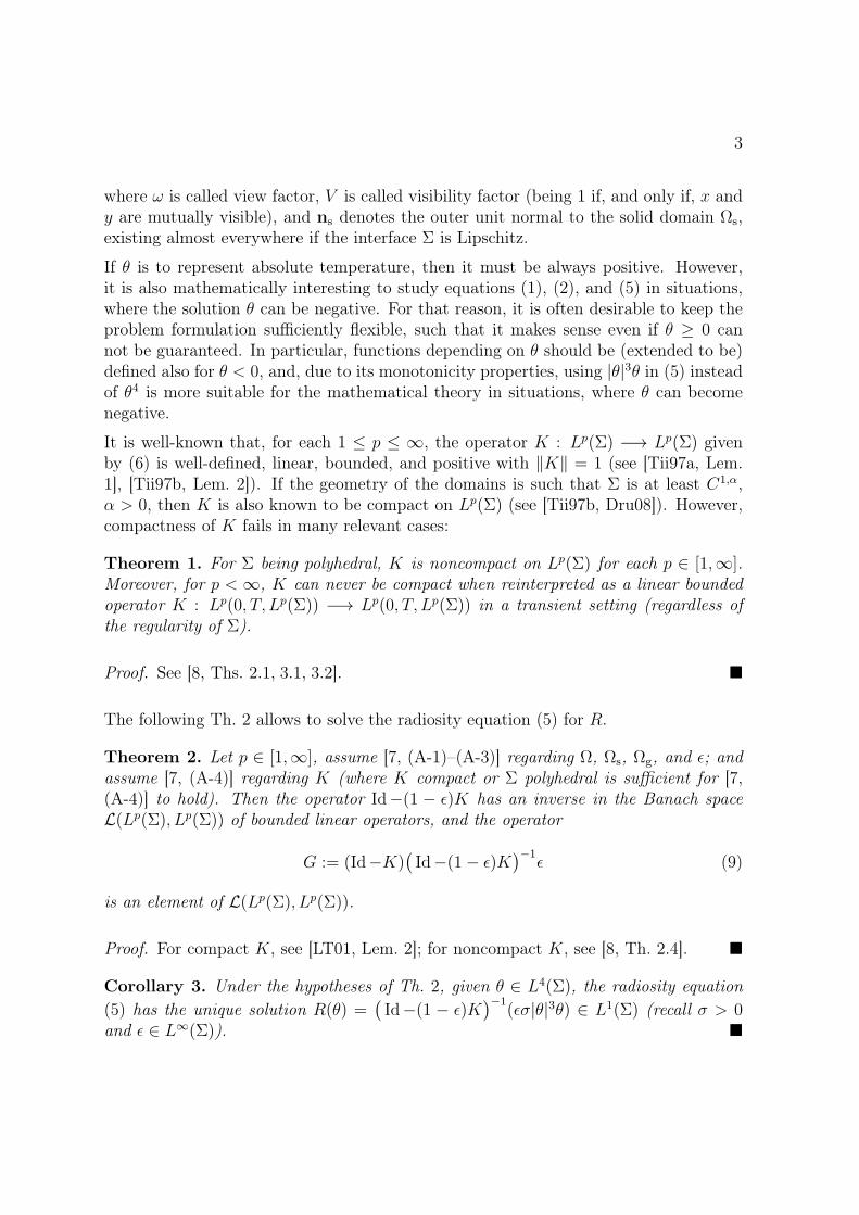
where ω is called view factor, V is called visibility factor (being 1 if, and only if, x andy are mutually visible), and ns denotes the outer unit normal to the solid domain Ωs,existing almost everywhere if the interface Σ is Lipschitz.

If θ is to represent absolute temperature, then it must be always positive. However,it is also mathematically interesting to study equations (1), (2), and (5) in situations,where the solution θ can be negative. For that reason, it is often desirable to keep theproblem formulation sufficiently flexible, such that it makes sense even if θ ≥ 0 cannot be guaranteed. In particular, functions depending on θ should be (extended to be)defined also for θ < 0, and, due to its monotonicity properties, using |θ|3θ in (5) insteadof θ4 is more suitable for the mathematical theory in situations, where θ can becomenegative.

It is well-known that, for each 1 ≤ p ≤ ∞, the operator K : Lp(Σ) −→ Lp(Σ) givenby (6) is well-defined, linear, bounded, and positive with ‖K‖ = 1 (see [Tii97a, Lem.1], [Tii97b, Lem. 2]). If the geometry of the domains is such that Σ is at least C1,α,α > 0, then K is also known to be compact on Lp(Σ) (see [Tii97b, Dru08]). However,compactness of K fails in many relevant cases:

Theorem 1. For Σ being polyhedral, K is noncompact on Lp(Σ) for each p ∈ [1,∞].Moreover, for p < ∞, K can never be compact when reinterpreted as a linear boundedoperator K : Lp(0, T, Lp(Σ)) −→ Lp(0, T, Lp(Σ)) in a transient setting (regardless ofthe regularity of Σ).

Proof. See [8, Ths. 2.1, 3.1, 3.2].

The following Th. 2 allows to solve the radiosity equation (5) for R.

Theorem 2. Let p ∈ [1,∞], assume [7, (A-1)–(A-3)] regarding Ω, Ωs, Ωg, and ε; andassume [7, (A-4)] regarding K (where K compact or Σ polyhedral is sufficient for [7,(A-4)] to hold). Then the operator Id−(1 − ε)K has an inverse in the Banach spaceL(Lp(Σ), Lp(Σ)) of bounded linear operators, and the operator

G := (Id−K)(Id−(1− ε)K

)−1ε (9)

is an element of L(Lp(Σ), Lp(Σ)).

Proof. For compact K, see [LT01, Lem. 2]; for noncompact K, see [8, Th. 2.4].

Corollary 3. Under the hypotheses of Th. 2, given θ ∈ L4(Σ), the radiosity equation(5) has the unique solution R(θ) =

(Id−(1 − ε)K

)−1(εσ|θ|3θ) ∈ L1(Σ) (recall σ > 0

and ε ∈ L∞(Σ)).

4

Using (9) together with the Stefan-Boltzmann law and Kirchhoff’s law, one easily ob-tains (cf. [7, (15)])

R(θ)− J(θ) = G(σ|θ|3θ) on Σ, (10)

such that (4) becomes(κ(x, θ)∇ θ

)Ωg

·ng +G(σ|θ|3θ) =(κ(x, θ)∇ θ

)Ωs

·ng on Σ. (11)

Assuming the domain Ω to be exposed to a black body environment (e.g. a large isother-mal room) radiating at θext (given absolute temperature), the Stefan-Boltzmann lawprovides the outer boundary condition

κ(x, θ)∇ θ · ns − σ ε (θ4ext − |θ|3θ) = 0 on ∂Ω. (12)

1.1.2 Optimal Control of Heat Sources

When modeling heat transfer for industrial applications such as crystal growth, one isusually not merely interested in determining the temperature distribution θ, but oneaims at optimizing θ according to a suitable objective functional. For example, duringsublimation growth of silicon carbide, small horizontal temperature gradients in the gasdomain Ωg are desirable to avoid defects of the growing crystal, while sufficiently largevertical temperature gradients are required to guarantee a material transport from thesilicon source to the seed crystal [SKM+00, MZPD02]. This background led to theoptimal control problem considered in [3]:

minimize J(θ, u) :=1

2

∫Ωg

‖∇ θ − z‖22 +ν

2

∫Ωs

u2 (13a)

subject to system (14) with f =

u on Ωs,

0 on Ωg,(13b)

and 0 < ua ≤ u ≤ ub in Ωs, (13c)

where z : Ωg −→ R3 is a given desired distribution for the temperature gradient, ν > 0is a regularization parameter, and system (14) is the summarized stationary model ofSec. 1.1.1, namely

− div(κ(x, θ)∇ θ

)= f(x) in Ω, (14a)(

κ(x, θ)∇ θ)Ωg

·ng +G(σ|θ|3θ) =(κ(x, θ)∇ θ

)Ωs

·ng on Σ, (14b)

κ(x, θ)∇ θ · ns − σ ε (θ4ext − |θ|3θ) = 0 on ∂Ω, (14c)

an integro-differential boundary value problem for the unknown θ : Ω −→ R. In par-ticular, (13b) imposes the condition of no heat sources in the gas region Ωg, motivated

5

by the application of induction heating. The control constraints (13c) reflect the factthat only heating (and no cooling) is considered, and they take into account that,due to technical limitations, an actual heating device can not produce heat sources ofarbitrarily large values.

Actually, from the point of view of the application, a control problem like (13), wherethe heat sources f are controlled directly, is only the first step. In practice, the heatsources are generated by a heating mechanism such as induction heating, i.e. f itself isagain the solution to some equation. A coupled system, where f is obtained as a solutionto Maxwell’s equations describing induction heating has been solved numerically in thecontext of industrial applications in [2, 5], which will be elaborated upon in Sections1.1.3, 1.1.4, and 1.1.5 below. Moreover, a control problem for such a coupled systemhas been solved numerically in [1], cf. Sec. 1.1.3 below.

The mathematical theory of (13) obviously requires a theory for the existence, unique-ness, and regularity of solutions to (14). Results regarding the existence, uniqueness,and regularity of solutions to (14) and also of solutions to the transient variant of (14)are surveyed in [7]. The essence of these results is the existence and uniqueness ofweak solutions to (14) and its transient counterpart under suitable hypotheses, wherestronger hypotheses can guarantee, in particular, the continuity of the weak solution,see [7, Ths. 9,12] for details. Here, only [7, Ths. 9] is reproduced as Th. 6 below, as itis technically easier to state and relevant to the stationary control problem (13). Still,we need some preparations:

Notation 4. For p, q ∈ [1,∞], let

V p,q(Ω) :=u ∈ W 1,p(Ω) : u ∈ Lq(Σ ∪ ∂Ω)

, (15)

simply writing u instead of tr(u) when considering u on Σ ∪ ∂Ω, suppressing the traceoperator tr.

Definition 5. Define θ ∈ V s,4(Ω) for some s ∈ [1,∞] to be a weak solution to (14) if,and only if,∫

Ω

κ(·, θ)∇ θ · ∇ψ +

∫∂Ω

σε|θ|3θψ +

∫Σ

G(σ|θ|3θ)ψ =

∫Ω

fψ +

∫∂Ω

σεθ4extψ (16)

for each ψ ∈ V s′,∞(Ω), where s′ ∈ [1,∞] is the conjugate exponent to s, i.e. 1s+ 1

s′= 1.

Theorem 6. Assume [7, (A-1)–(A-4), (A-6)–(A-11)].

(a) If f ∈ Lp(Ω), where p > 97

or just p > 1 under the additional assumption that Σis C1,α, α > 0, then (14) has a weak solution θ. If f ≥ 0, then θ ≥ ess inf θext.Moreover, regarding the regularity of θ, if p ≥ 3

2and θext ∈ L8(∂Ω), then |θ|r ∈

6

W 1,2(Ω) for each r ∈ [1,∞[. If p ∈]97, 32[ and θext ∈ L8p/(3−p)(∂Ω), then θ ∈

V 2,2p/(3−2p)(Ω) with 2p/(3 − 2p) > 6. If Σ is C1,α, α > 0, p ∈ [65, 97] and θext ∈

L8p/(3−p)(∂Ω), then θ ∈ V 2,(9−5p)/(3−2p)(Ω) with 5 ≤ (9− 5p)/(3− 2p) ≤ 6. If Σ isC1,α, α > 0, p ∈]1, 6

5[ and θext ∈ L8p/(3−p)(∂Ω), then θ ∈ V 3p/(3−p),(9−5p)/(3−2p)(Ω)

with 32< 3p/(3− p) < 2.

(b) If f ∈ L1(Ω), Σ is C1,α, α > 0, and ε < 1, then (14) has a weak solution θ ∈⋂s∈[1, 3

2[ V

s,4(Ω).

(c) If θext ∈ L∞(∂Ω), f ∈ Lp(Ω) with p > 32, and all ∂Ωi are C1, then (14) has a

weak solution θ ∈ W 1,q with q := 2p > 3 (in particular, the solution is Höldercontinuous, θ ∈ Cγ(Ω), γ > 0). This solution is unique provided κ is piecewiseLipschitz continuous (cf. [7, (A-6), Th. 9(c)]).

Proof. For (a) see [Dru09, Th. 5.1], for (b) see [Dru09, Th. 6.1], and for (c) see [DKS+11,Lem. 3.6] and its proof.

Definition 7. Under the assumptions of Th. 6(c), define the control-to-state operatorS : L2(Ωs) −→ W 1,q(Ω) ⊆ Cγ(Ω) ⊆ L∞(Ω) (q > 3 as in Th. 6(c), γ > 0), u 7→ θ,

assigning to u ∈ L2(Ωs) the unique weak solution θ of (14) with f :=

u on Ωs,

0 on Ωg,

provided by Th. 6(c).

Definition 8. Employing the control-to-state operator of Def. 7, and letting

Uad :=u ∈ L∞(Ωs) : ua ≤ u ≤ ub

, (17)

(θ, u) ∈ W 1,q(Ω)×Uad (q > 3 as in Th. 6(c)) is called an optimal control for (13) if, andonly if, θ = S(u), and u minimizes the reduced objective functional

j : L2(Ωs) −→ R+0 , j(u) := J

(S(u), u

)(18)

on Uad.

—

The following theorem provides the existence of an optimal control for (13) under thesimplifying assumption of θ-independent κ:

Theorem 9. Under the assumptions of Th. 6(c) plus z ∈ L2(Ωg,R3), ua, ub ∈ L∞(Ωs),0 < ua ≤ ub, κ θ-independent, and ess inf θext > 0, there exists an optimal control (θ, u)for (13).

Proof. See [3, Th. 5.2].

7

Next, the differentiability of the control-to-state operator is considered as well as first-order necessary optimality conditions for (13), which are related to weak solutions tothe linearized form of (14):

Definition 10. Under the assumptions of Th. 6(c) plus ess inf θext > 0, let u ∈ L2(Ωs),u ≥ 0, θ := S(u) ∈ W 1,q(Ω) with q > 3 as in Th. 6(c). Given F in the dual of W 1,q′(Ω)(q′ the conjugate exponent to q), a function θ ∈ W 1,q(Ω) is called a weak solution tothe linearized form of (14) (or (16)) with right-hand side F if, and only if,∫

Ω

κ(·, θ)∇ θ · ∇ψ +

∫Ω

∂κ

∂θ(·, θ)θ∇ θ · ∇ψ

+ 4

∫∂Ω

σε|θ|3θψ + 4

∫Σ

G(σ|θ|3θ)ψ = F(ψ) (19)

for each ψ ∈ W 1,q′(Ω) (recall G : L∞(Σ) −→ L∞(Σ) according to Th. 2).

Theorem 11. Under the assumptions of Th. 6(c) plus ess inf θext > 0, and κ beingpiecewise C1 with bounded derivative in the sense of [7, (A-6), (A-15)] (θ-independenceis not needed here), the control-to-state operator of Def. 7 is Fréchet differentiable onL2+(Ωs) := u ∈ L2(Ωs) : u > 0. Moreover, for u ∈ L2

+(Ωs), θ = S(u), and u ∈ L2(Ωs),one has θ := S ′(u)(u) given by the weak solution to the linearized form of (14) (i.e. of(19)) with right-hand side F(ψ) := Fu(ψ) :=

∫Ωsuψ.

If z ∈ L2(Ωg,R3), ua, ub ∈ L∞(Ωs), 0 < ua ≤ ub, then (θ, u) ∈ W 1,q(Ω)× Uad (q > 3 asin Th. 6(c)) being an optimal control for (13) implies the necessary condition

j′(u)(u− u) = 〈∇ θ − z,∇ θ〉L2(Ωg) + ν〈u, (u− u)〉L2(Ωs) ≥ 0 for each u ∈ Uad, (20)

with j as in (18), θ = S(u), and θ = S ′(u)(u− u).

Proof. See [3, Th. 7.1] and [7, Th. 18]. The proof is based on the implicit functiontheorem and makes use of [DKS+11, Th. 4.4] which, under the above hypotheses, pro-vides a unique weak solution θ ∈ W 1,q(Ω) to (19), where this solution also satisfies‖θ‖W 1,q(Ω) ≤ c ‖F‖ for some c > 0.

1.1.3 Induction Heating: Model and Control

As stated before, from the point of view of industrial applications such as crystal growth,a control problem like (13), where the heat sources f are controlled directly, is only thefirst step. In practice, the heat sources are generated by a heating mechanism suchas induction heating, i.e. f itself is again the solution to some equation. A controlproblem, where f is obtained as a solution to Maxwell’s equations describing induction

8

heating, has been treated numerically in [1] for axisymmetric geometries. In [1], the heatsources f are obtained due to induction heating, generated by finitely many coil ringslocated outside the domain Ω. The heat sources are numerically computed according tothe following model, where all materials in Ωs are considered as potential conductors,whereas Ωg is treated as a perfect insulator (see [KPS04, Sec. 2.6] for details; due tothe axisymmetry, cylindrical coordinates (r, z) are used):

f(r, z) =|j(r, z)|2

2σc(r, z), (21)

j =

−iω σc φ + σc vk

2πrin the k-th coil ring,

−iω σc φ in Ωs,(22)

where σc denotes the electrical conductivity, vk is the voltage imposed in the kth coilring, ω is the common angular frequency of the imposed voltages, and i is the imagi-nary unit. The potential φ is determined from the following system of elliptic partialdifferential equations:

− ν div∇(rφ)

r2= 0 in Ωg, (23a)

− ν div∇(rφ)

r2+i ωσcφ

r=σc vk2πr2

in the k-th coil ring, (23b)

− ν div∇(rφ)

r2+i ωσcφ

r= 0 in Ωs, (23c)

where ν denotes the magnetic reluctivity. The system (23) is completed by the interfaceconditions (

νΩi

r2∇(rφ)Ωi

)• nΩi

=

(νΩj

r2∇(rφ)Ωj

)• nΩi

, (24)

and the assumption that φ = 0 both on the symmetry axis r = 0 and sufficiently farfrom the growth apparatus (imposed as Dirichlet boundary condition).

The domain used for the numerical computations of [1] represents an apparatus forsilicon carbide single crystal growth via sublimation by physical vapor transport. Theprecise domain and its dimensions are provided in [1, Figs. 1,3]. During sublimationgrowth of silicon carbide, small horizontal temperature gradients in the gas domain Ωg

(more precisely in the part of Ωg close to the surface of the growing crystal) are desirableto avoid defects of the growing crystal, while sufficiently large vertical temperaturegradients are required to guarantee a material transport from the silicon source to theseed crystal [SKM+00, MZPD02].

The control problem solved numerically in [1] is similar to (13). However, for the opti-mization of the temperature field θ in [1], the heat sources were not controlled directly

9

as in (13), but they were computed according to (21) – (24), whereas the quantitiesheating power P , vertical upper rim zrim of the induction coil (cf. [1, Fig. 1]), and thefrequency f = ω/(2π) of the heating voltage were used as control parameters, which ismore realistic from the point of view of the considered crystal growth application. Thecontrol parameters, thus, result in a temperature distribution θ(P, zrim, f) via (21) –(24) and (14) (see [1] for details; one should not get confused by the fact that f = ω/(2π)denotes the frequency in [1] and not, as in (21) and previous equations above, the heatsources occurring on the right-hand side of the heat equation).

While [1, Fig. 7(a)] depicts the numerically computed temperature field for a generic,unoptimized situation as a reference, the objective functional minimized in [1, Fig. 7(b)]is

Fr(θ) :=

(∫Γ

2π r ∂rθ(r, z)2 dr

)1/2

, (25)

aiming at minimizing the radial temperature gradient on the lower surface Γ of thegrowing SiC crystal. The objective functional minimized in [1, Fig. 7(c)] is

1

2Fr(θ)−

1

2Fz(θ), Fz(θ) :=

(∫A

2π r ∂zθ(r, z)2 d(r, z)

)1/2

, (26)

aiming at minimizing the radial temperature gradient on Γ, while simultaneously max-imizing the vertical temperature gradient inside the region A between the SiC crystaland the SiC powder, to guarantee material transport from the powder to the crystal(cf. [1, Fig. 2]).

The optimization is subject to a number of state constraints on θ, motivated by thecrystal growth application: (a) The maximal temperature in the apparatus must notsurpass a prescribed bound θmax; (b) the temperature at the crystal surface Γ needsto stay within a prescribed range [θmin,Γ, θmax,Γ]; (c) the temperature gradient betweensource and seed must be negative, and must not surpass a prescribed value ∆max < 0:

maxΩ

(θ) ≤ θmax, (27a)

θmin,Γ ≤ minΓ

(θ) ≤ maxΓ

(θ) ≤ θmax,Γ, (27b)

maxA

(∂zθ) ≤ ∆max < 0. (27c)

A Nelder-Mead method was used for the numerical optimization as described in [1, Sec.3]. The simulation software WIAS-HiTNIHS (cf. Sec. 1.1.5 below) was used for therequired repeated numerical solution of the coupled state system (14), (21) – (24).

The main difference between the generic solution of [1, Fig. 7(a)] and the optimizedsolutions shown in [1, Figs. 7(b),(c)] is the gained homogeneity of the temperature inside

10

the SiC crystal in the optimized solutions (favorable with respect to low thermal stressand few crystal defects) as well as the isotherms below the crystal’s surface becomingmore parallel to that surface (as intended by the minimization of Fr(θ)). As expected,in [1, Fig. 7(c)], the maximization of Fz(θ) leads to an increased number of isothermsbetween the crystal and the source powder. Summarizing the results, the radial andthe vertical gradient can be effectively tuned simultaneously.

In [1, Figs. 4–6], the paper [1] also provides contour plots of the values of the objectivefunctionals depending on the control parameters θ(P, zrim, f), illustrating the effect ofthe state constraints as well as the location of the numerically determined optimalcontrols.

1.1.4 Anisotropic Thermal Conductivity

The included articles [2, 4] deal with the numerical simulation of conductive-radiativeheat transfer in the presence of anisotropic thermal conductivity. This is relevant tocrystal growth applications since it is not unusual for the thermal insulation of growthapparatus to possess an anisotropic thermal conductivity (e.g. in the case of graphitefelt, where the fibers are aligned in one particular direction). In generalization of (2),stationary heat conduction in anisotropic materials is described by

− div(Km(θ)∇ θ

)= fm in Ωm (m ∈M), (28)

where the symmetric and positive definite matrix Km represents the thermal conduc-tivity tensor in material m, fm represents heat sources in material m, Ωm is the domainof material m, and M is a finite index set. The papers [2, 4] consider the case wherethe thermal conductivity tensor is a diagonal matrix with temperature-independentanisotropy, i.e.

Km(θ) =(κmi,j(θ)

), where κmi,j(θ) =

αmi κ

miso(θ) for i = j,

0 for i 6= j,(29)

κmiso(θ) > 0 being the thermal conductivity of the isotropic case (allowed to depend onthe temperature θ), and αm

i > 0 being anisotropy coefficients. The material domainsΩm are supposed to satisfy the geometric assumptions [4, (A-1)], restated below:

Assumption 12. Ω =⋃

m∈M Ωm, Ωm1 ∩ Ωm2 = ∅ for each (m1,m2) ∈ M2 such thatm1 6= m2, and each of the sets Ω, Ωm, m ∈ M , is a nonvoid, connected, polyhedral,bounded, and open subset of R2 (even though (28) holds in three dimensions, in theaxisymmetric context of [2, 4], it suffices to consider the two-dimensional case, cf. [4,Sec. 3.6]).

11

The modification of the interface condition (4) for interfaces between anisotropic ma-terials m1 and m2, m1 6= m2, reads(

Km1(θ)∇ θ)Ωm1

•nm1 =(Km2(θ)∇ θ

)Ωm2

•nm1 on Ωm1 ∩ Ωm2 , (30)

where the anisotropic materials are taken as opaque, such that no radiative contribu-tions R, J are present in (30). The unit normal vector nm1 in (30) points from materialm1 to material m2.

In [4], a finite-volume discretization suitable for the numerical solution of (29), (30) withsuitable boundary conditions is developed. The presented scheme was implemented inthe software WIAS-HiTNIHS and used to compute the numerical results in [2, 4]. Anadmissible discretization of material domain Ωm, m ∈ M , consists of a finite familyΣm := (σm,i)i∈Im of subsets of Ωm satisfying the following Assumptions 13 and 15.

Assumption 13. For each m ∈M , Σm = (σm,i)i∈Im forms a finite conforming triangu-lation of Ωm. In particular, for each i ∈ Im, σm,i is an open triangle. Moreover, lettingI :=

⋃m∈M Im, Σ := (σi)i∈I forms a conforming triangulation of Ω.

—

For each σm,i, let V (σm,i) =vmi,j : j ∈ 1, 2, 3

denote the set of vertices of σm,i, and

let V :=⋃

m∈M, i∈Im V (σm,i) be the set of all vertices in the triangulation. One can thendefine the control volumes as the Voronoï cells with respect to the vertices. Using ‖ · ‖2to denote Euclidean distance, define

for all v ∈ V : ωv :=x ∈ Ω : ‖x− v‖2 < ‖x− z‖2 for each z ∈ V \ v

, (31a)

for all m ∈M : ωm,v := ωv ∩ Ωm, Vm := z ∈ V : ωm,z 6= ∅. (31b)

Letting T := (ωv)v∈V , Tm := (ωm,v)v∈Vm , m ∈ M , T forms a partition of Ω, and Tm

forms a partition of Ωm.

Remark 14. Since T is a Voronoï discretization, each intersection ∂ωv ∩ ∂ωz, (v, z) ∈V 2, v 6= z, is contained in the set x ∈ Ω : ‖v − x‖2 = ‖z − x‖2. In particular,z−v

‖z−v‖2 = nωv ∂regωv∩∂regωz , where ∂reg denotes the regular boundary of a polyhedralset, i.e. the points of the boundary, where a unique outer unit normal vector exists,∂reg∅ := ∅; and nωv ∂regωv∩∂regωz is the outer unit normal to ωv restricted to the face∂regωv ∩ ∂regωz (see [4, Fig. 2]).

Assumption 15. For each m ∈M , the triangulation Σm has the constrained Delaunayproperty: If Vm :=

⋃i∈Im V (σm,i); then, for each (v, z) ∈ V 2

m such that v 6= z, thefollowing conditions (a) and (b) are satisfied:

(a) If the boundaries of the Voronoï cells corresponding to v and z have a one-dimen-sional intersection, then the line segment [v, z] is an edge of at least one σ ∈ Σm.

12

(b) If [v, z] is an edge of at least one σ ∈ Σm, then the boundaries of the correspondingVoronoï cells have a nonempty intersection.

Due to the two-dimensional setting, the constrained Delaunay property can be expressedequivalently in terms of the angles in the triangulation: For each m ∈ M , if γ is aninterior edge of the triangulation Σm, and α and β are the angles opposite to γ, thenα + β ≤ π. If γ ⊆ ∂Ωm is a boundary edge of Σm, and α is the angle opposite γ, thenα ≤ π/2. Also see [4, Fig. 2].

Remark 16. Using Rem. 14, it is not hard to show that Assumptions 13 and 15 implythe following assertions (a) and (b):

(a) For each m ∈ M , the set Vm defined in (31b) is identical to the set Vm defined inAssumption 15.

(b) Let Γ be a one-dimensional material interface: Γ = ∂Ωm ∩ ∂Ωm. For each v ∈ V ,if some ωv has a one-dimensional intersection with the interface Γ, then it lies onboth sides of the intersection; in other words, ∂regωm,v ∩ Γ = ∂regωm,v ∩ Γ.

—

As usual, the finite volume scheme for (28), (30) is constructed by integrating (28) overωm,v, applying the Gauss-Green integration theorem to obtain

−∫∂ωm,v

(Km(θ)∇ θ) • nωm,v =

∫ωm,v

fm (32)

(where nωm,v denotes the outer unit normal vector to ωm,v), and by using (30) followedby suitable approximations for the integrals. In the context of (14), the construction andfurther references can be found in [7, Sec. 4]. The novelty of [4] lies in the approximationof the heat flux integrals

∫∂ωm,v∩Ωm

(Km(θ)∇ θ) • nωm,v in the presence of anisotropicthermal conductivity, so only the main particularities of this approximation are brieflyincluded below.

Notation 17. For each m ∈ M and each (v, w) ∈ M2, let γm,v,w := ∂ωm,v ∩ ∂ωm,w

denote the interface of the two Voronoï cells inside the material domain Ωm (of course,in general, γm,v,w can be empty).

—

For the approximation of∫∂ωm,v∩Ωm

(Km(θ)∇ θ)• nωm,v , the set ∂ωm,v∩Ωm is partitionedfurther, namely into the interfaces with all neighboring Voronoï cells. Up to null setswith respect to one-dimensional Lebesgue measure λ1

∂ωm,v ∩ Ωm =⋃

w∈nbm(v)

γm,v,w, (33)

13

where nbm(v) := w ∈ Vm \ v : λ1(γm,v,w) 6= 0 is the set of m-neighbors of v (cf. [4,Fig. 3]).

Using (33), it remains to approximate (Km(θ)∇ θ) • nωm,v on γm,v,w. According to theassumed form (29) of the Km(θ), the approximation can be broken down into two parts:(a) Approximation of the temperature-dependent, isotropic part. (b) Approximationof the temperature-independent, anisotropic part.

Approximation of the temperature-dependent, isotropic part

The quantity κmiso(θ) on γm,v,w is approximated by the mean

κmiso(θ)γm,v,w≈1

2

(κmiso(θv) + κmiso(θw)

)(34)

(cf. remark after [4, (14)]).

Approximation of the temperature-independent, anisotropic part

For the anisotropic part, it remains to approximate (Am∇ θ) • nωm,v on γm,v,w, whereAm is the constant diagonal matrix

Am = (ami,j), ami,j :=

αmi for i = j,

0 for i 6= j.(35)

The approximation of [4] is devised such that it is exact provided θ is affine on eachσ ∈ Σ and provided Σ has the strong Delaunay property (all angles are less than orequal to π/2). If θ is affine on σ ∈ Σ, then

∇ θσ=∑

v∈V (σ)

θ(v) ∇φσ,v, (36)

where φσ,v : σ −→ [0, 1], v ∈ V (σ), are the affine coordinates on the triangle σ withrespect to its 3 vertices.

Given m ∈M , (v, w) ∈ V 2m, v 6= w, such that [v, w] is an edge of some σ ∈ Σm, let

Σm,v,w :=σ ∈ Σm : v, w ⊆ V (σ)

(37)

be the set of triangles in Σm having [v, w] as an edge. Since Σm is a conformingtriangulation of Ωm by Assumption 13, if [v, w] is a boundary edge, then Σm,v,w hasprecisely one element; otherwise, it has precisely two elements, lying on different sidesof [v, w]. For each σ ∈ Σm,v,w, let Hv,w,σ be the half-space that lies on the same side of

14

the line through [v, w] as σ. Even though Assumption 15 guarantees λ1(γm,v,w) 6= 0, [4,Fig. 3] shows that γm,v,w can lie entirely on one side of [v, w]. However, letting

Σγm,v,w :=σ ∈ Σm,v,w : λ1(Hv,w,σ ∩ γm,v,w) 6= 0

, (38)

one can decompose γm,v,w according to (cf. [4, Fig. 3])

γm,v,w =⋃

σ∈Σγm,v,w

σ ∩ γm,v,w. (39)

Using (36) together with Rem. 14 yields, for each σ ∈ Σγm,v,w :

(Am∇ θ)σ •nωv γm,v,w=∑

v∈V (σ)

θ(v) (Am∇φσ,v) •w − v

‖w − v‖2. (40)

Together with (34) and (39), (40) provides the approximation of the normal heat fluxacross γm,v,w (cf. (41) below). Formula (40) constitutes the key difference to and im-provement over previously published schemes (see Introduction and paragraphs follow-ing (20) in [4]).

Combining the temperature-dependent and temperature-independent parts

Combining the approximations of the temperature-dependent and the temperature-in-dependent parts, i.e. combining (34), (39), and (40) yields∫

γm,v,w

(Km(θ)∇ θ) • nωm,v

≈∑

σ∈Σγm,v,w

1

2

(κmiso(θv) + κmiso(θw)

)∑

v∈V (σ)

θv (Am∇φσ,v) •w − v

‖w − v‖2λ1(Hv,w,σ ∩ γm,v,w).

(41)

Numerical Results Using the New Scheme

Numerical results verifying the new scheme in comparison with exactly computableclosed-form solutions can be found in [4, Sec. 4.2], showing second-order convergence ina single-material domain and first-order convergence in a multi-material domain withdiscontinuous thermal conductivity coefficients.

In [2], the new scheme is employed to compute temperature fields in realisticly modeledcrystal growth apparatus with thermally anisotropic insulation material. The numerical

15

results in [2, Sections 4.2 and 5] show that, depending on the insulation’s orientation,even a moderate anisotropy in the insulation can result in temperature variations ofmore than 100 K at the growing crystal’s surface, which need to be taken into accountfor an accurate simulation as well as for the design of the growth apparatus.

1.1.5 Numerical Simulation Software WIAS-HiTNIHS1

Except [3, 6, 8], all included papers present numerical simulation results computedusing the software WIAS-HiTNIHS. At WIAS Berlin, I was the head developer ofWIAS-HiTNIHS in the period 1997 – 2006. Since I left WIAS Berlin, the role of headdeveloper was taken over by Dr. Olaf Klein.

WIAS-HiTNIHS constitutes a tool for both stationary and transient simulations ofheat transport in axisymmetric technical systems that are subject to heating by in-duction. The simulator accounts for heat transfer by radiation through cavities, andit allows for changes in the material parameters due to the rising temperature, e.g.employing temperature-dependent laws of thermal and electrical conductivity. Usinga band model, WIAS-HiTNIHS can treat materials as semi-transparent. Anisotropicthermal conductivity can be accounted for during the computations as in [2, 4]. Itis also possible to use WIAS-HiTNIHS just to compute axisymmetric magnetic scalarpotentials and the resulting heat sources. An optimization module allows the controlof parameters such as heating power and coil position with the objective of minimizingfunctionals such as the max-norm of the radial temperature gradient in a neighbor-hood of the growing crystal’s surface as in [1]. The simulator is designed to deal withcomplicated axisymmetric setups having a polygonal 2-dimensional projection.

From a more abstract perspective, WIAS-HiTNIHS is a solver for two-dimensionalpotentially nonlinear elliptic and parabolic PDE in both Cartesian and cylindrical co-ordinates. Multi-material, polyhedral domains are allowed, and all material functionscan depend nonlinearly on the solution. Fourier law type interface conditions are imple-mented as well as nonlocal radiative interface conditions. Implemented outer boundaryconditions include time- and space-dependent Dirichlet conditions, Neumann and Robinconditions, emission conditions, and nonlocal radiative conditions. A shape optimiza-tion module enables numerical PDE-driven shape optimization via optimal control of ashape function on a (larger) fixed domain as described in [9].

The PDE solver in WIAS-HiTNIHS employs a finite volume discretization [7, Sec. 4].WIAS-HiTNIHS is based on the program package pdelib [FKL01], it employs the gridgenerator Triangle [She96, She02] to produce constrained Delaunay triangulations ofthe domains, and it uses the sparse matrix solver PARDISO [SG04, SGF00] to solvethe linear system arising from the finite volume scheme.

1High Temperature Numerical Induction Heating Simulator; pronunciation: ∼hit-nice.

16

In the included paper [5], WIAS-HiTNIHS is used to aide the industrial applicationof liquid encapsulated Czochralski crystal growth of GaAs under the influence of atraveling magnetic field. It is used to compute electromagnetic fields as well as temper-ature fields in realistic growth apparatus, assessing the influence of the Lorentz force onthe melt, e.g. regarding the damping of the temperature oscillations below the crystal,desirable for high-quality growth.

1.2 Crack Propagation

The included paper [6] is aimed at improving the understanding of brittle fractureformation and propagation in materials. While the classical theory of Griffith [Gri21]constitutes the foundation of modern understanding of brittle fracture, it still has anumber of significant shortcomings: Griffith theory does not predict crack initiationand path and it suffers from the presence of unphysical stress singularities. Whilethe former problem is addressed, e.g., in [FM98, DFT05], and the latter problem isaddressed, e.g., in [SMS05], [6] is directed at including the ideas of [SMS05] for theremoval of stress singularities into the framework of [FM98, DFT05].

The approach of [FM98, DFT05] has the advantage that it does not need to prescribe thepresence of a crack or its path a priori, but the potential crack as well as its path are partof the problem’s solution. It is founded on the global minimization of energy functionalsacting on spaces of functions of bounded variations, where the cracks are related tothe discontinuity sets of such functions. The model of [6] formulates modified energyfunctionals that account for molecular interactions in the vicinity of crack tips and thecohesive forces in the spirit of [SMS05]. In contrast to [FM98, DFT05], the model alsoallows for crack reversibility and considers local minimizers of the energy functionals,employing different time scales. Solving the model for a simple one-dimensional examplewith a dead load, it is shown that the local energy minimization yields the physicallyexpected result in a situation where the global minimization according to [FM98] fails.

The goal in [6] is to model a strained and cracked body quasistatically using a time- andspace-dependent function u, representing the body’s displacement field with respect toan uncracked reference configuration Ω ⊆ RN , N ∈ 1, 2, 3, assumed to be nonempty,bounded, open, connected, with Lipschitz boundary ∂Ω. The considerations in [6]culminate in the formulation of two versions of a quasistatic evolution model, onebased on global energy minimization in [6, Sec. 2.5.5] and one based on local energyminimization in [6, Sec. 2.5.6]. Both versions will be restated here, followed in each caseby summaries of the involved concepts. Previously unexplained notation occurring inthe following Def. 18 will also be made clear after the definition statement below.

Definition 18. Let T > 0. A quasistatic evolution of globally minimizing energyconfigurations (QEGMEC) is a function u : [0, T ] −→ SBV ∞(Ω,RN) satisfying the

17

following conditions:

(a) For each t ∈ [0, T ]: u(t) ∈ AD(t).

(b) For each t ∈ [0, T ]: E(t)(uu(t)) ≤ E(t)(uv) for every v ∈ AD(t).

(c) Wext(t)(u)−Wext(s)(u) = E(t)(u)− E(s)(u) for each (s, t) ∈ [0, T ]2, s < t.

—

In Def. 18, the variables s, t ∈ [0, T ] represent time, SBV ∞(Ω,RN) := SBV (Ω,RN) ∩L∞(Ω,RN), SBV (Ω,RN) denoting the space of special functions of bounded variation,and the set AD(t) in Def. 18(a),(b) is the set of admissible displacement fields satisfyinga Dirichlet boundary condition on ∂DΩ ⊆ ∂Ω (see [6, Sec. 2.5.1, Sec. 2.3]):

AD(t) :=u ∈ SBV ∞(Ω,RN) : tr∂DΩ u = uD(t) ∈ L∞(∂DΩ,RN) given

. (42)

The model requires u(t) ∈ L∞(Ω,RN), since unbounded displacements are not physi-cally reasonable, and the requirement u(t) ∈ SBV (Ω,RN) is reasonable in the contextof crack modeling as explained in [6, Sec. 2.1.2]. In particular, for a fixed time t, theset Γ(u, r) ⊆ Ω of present cracks can be defined by

Γ(u, r) := r−11 ∪x ∈ Ju :

([u](x)

)• nJu(x) > 0

, (43)

where Ju is the so-called jump set of u := u(t) ∈ SBV (Ω,RN), nJu denotes the normalvector with respect to Ju,

[u] : Ju −→ RN , [u](x) := u+(x)− u−(x), (44)

u+ and u− being the one-sided limits of u with respect to Ju. Moreover, the crackreversibility function r : Ω −→ 0, 1 occurring in (43) is an accounting tool that, foreach x ∈ Ω, records if there is an irreversible crack at x or not: r(x) = 1 if, and onlyif, there is an irreversible crack at x (thus, if r(x) = 0, then there is either no crack atx, or there is a reversible crack at x). According to the model of [6], irreversibility istriggered by a crack having opened more than a threshold value ath > 0. Thus, moreprecisely, r depends on time and space, r : [0, T ]× Ω → 0, 1, and, given u and ath,

ru(t, x) =

0 if

([u](t, x)

)• nJu(t)(x) < ath for all s ≤ t,

1 otherwise.(45)

In consequence, ru can be seen as a memory function for u: The energy at time t doesnot only depend on u(t), but also on ru(t), i.e. on the history of u. It is also noted that

18

the crack (43) is determined by u and r, i.e. it does not have to be specified separatelyas in Francfort-Marigo theory [FM98].

The functional E(t) in Def. 18(b),(c) represents the total energy at time t. As describedin [6, Sec. 2.4.5], there are several contributions to the total energy, namely the energyof the crack, the bulk energy, the energy of the body forces, and the energy of thesurface forces. Only the formula for determining the energy of the crack is new in [6,Sec. 2.4.1] and is summarized here (see [6, Sec. 2.4.2 – Sec. 2.4.4] for the remainingcontributions): The energy Ecr of the crack is defined by

Ecr(u, r) :=∫Γ(u,r)

κ(x,nΓ(x), [u](x), r(x)

)dHN−1(x), (46)

where HN−1 denotes the restriction of (N−1)-dimensional Hausdorff measure to Γ(u, r),and

κ : Ω× SN−1 × RN × 0, 1 −→ R+0 ∪ ∞ (47)

is a function modeling the material’s toughness, SN−1 denoting the (N−1)-dimensionalunit sphere. The dependence of κ on x and nΓ(x) describes the location- and direction-dependent toughness of the material. The dependence of κ on its third variable allowsto account for Barenblatt-type energies corresponding to cohesive forces depending onthe normal distance of the crack lips. Permitting κ to depend on the entire jump [u](x)instead of just on the jump in the normal direction allows to include energy barriers forslip dislocations (jumps of u parallel to the crack). The dependence on r(x) allows toaccount for crack reversibility: The idea is to use this as a switch for the dependenceof κ on its third variable: As cohesive forces should play no role once the crack hasbecome irreversible, κ should depend nontrivially on the third variable if, and only if,the fourth variable is 0. For an example of a toughness function κ based on a Lennard-Jones potential, see [6, (10),(11)] and [6, Fig. 2]. According to the reasoning in [6, Sec.2.4.1], κ should, at least, have the following properties:

(a) κ(x,n, z, r) <∞ for each (x,n, z, r) ∈ Ω× SN−1 ×RN ×0, 1 such that z •n ≥ 0.

(b) κ(x,n, z1, 1) = κ(x,n, z2, 1) for each (x,n, z1, z2) ∈ Ω× SN−1 ×RN ×RN such thatz1 • n ≥ 0 and z2 • n ≥ 0.

(c) For each (x,n) ∈ Ω× SN−1, the function z 7→ κ(x,n, z, 0) is continuous on the setz ∈ RN : 0 ≤ z • n ≤ ath.

(d) κ(x,n, z, 0) = κ(x,n, z, 1) for each (x,n, z) ∈ Ω× SN−1 ×RN such that z •n = ath.

—

Condition Def. 18(b) is the condition of global energy minimization (cf. [6, Sec. 2.5.2]):For each t ∈ [0, T ], u(t) needs to be a minimizer of the total energy E(t) among all

19

admissible v ∈ AD(t). Due to the presence of the reversibility function, to be able toformulate the condition at time t, one has to make use of the function u already definedfor times smaller than t: Let v ∈ AD(t) be an admissible displacement field at time t,and let u : [0, t[−→ SBV ∞(Ω,RN) be given. Then u can be extended to time t by v:

uv : [0, t] −→ SBV ∞(Ω,RN), uv(s) :=

u(s) for s < t,

v for s = t.(48)

Finally, condition Def. 18(c) states the energy balance: For each time interval, theincrement in stored energy plus the energy spent in crack increase (or recovered bycrack closure) needs to equal the work Wext of the external forces, where, in general,Wext has the three contributions listed in [6, Sec. 2.5.4].

We now come to the model of [6, Sec. 2.5.6], which is based on local energy minimization.It is restated as Def. 19, followed by further explanations.

Definition 19. Let T > 0. A quasistatic evolution of locally minimizing energy config-urations (QELMEC) is a function u : [0, T ] −→ SBV ∞(Ω,RN) satisfying the followingconditions:

(a) For each t ∈ [0, T ]: u(t) ∈ AD(t).

(b) For each t ∈ [0, T ], there is ε > 0 such that E(t)(uu(t)) ≤ E(t)(uv) for each v ∈ AD(t)satisfying ‖u(t)− v‖∞,1 < ε.

(c) There exists a finite sequence of times 0 = t0 < · · · < tn = T such that u is con-tinuous with respect to the ‖ · ‖∞,1-norm on each interval [tν−1, tν [, ν ∈ 1, . . . , n,and, for each ν ∈ 1, . . . , n, there is vν ∈ AD(tν) such that the map

uν : [tν−1, tν ] −→ SBV ∞(Ω,RN), uν(t) :=

u(t) for t < tν ,

vν for t = tν ,

is continuous with respect to the ‖·‖∞,1-norm on the entire closed interval [tν−1, tν ],and such that there is an admissible path pν ∈ Ptν

(vν , u(tν)

)connecting vν and

u(tν).

(d) Wext(t)(u)−Wext(s)(u) = E(t)(u)− E(s)(u) for each (s, t) ∈ [0, T ]2, s < t.

—

Conditions Def. 19(a),(d) were already present in Def. 18. Condition Def. 19(b) is thelocal analogue of the global minimization condition Def. 18(b): For each t ∈ [0, T ],

20

u(t) now needs to be a local minimizer of the total energy E(t) among all admissiblev ∈ AD(t), local with respect to the norm

‖u‖∞,1 := ‖u‖∞ + ‖∇ u‖1, (49)

where ∇u denotes the absolutely continuous part of the distributional derivative of uwith respect to Lebesgue measure (see [6, Sec. 2.5.3] regarding the choice or norm).

Condition Def. 19(c) states that the quasistatic evolution must be energetically ad-missible, where, for a fixed time t ∈ [0, T ], given u : [0, t[−→ SBV ∞(Ω,RN), the setPt(v1, v2) of admissible paths between states v1 and v2, (v1, v2) ∈ AD(t) × AD(t), isdefined as the set of maps p : [0, 1] −→ AD(t) continuous with respect to ‖ · ‖∞,1 suchthat p(0) = v1, p(1) = v2, and such that the map a 7→ E(t)

(up(a)

)is nonincreasing on

[0, 1]. According to [6, Sec. 2.5.3], condition Def. 19(c) arises from considering differentscales for the time dependence: First, assume that the local minima in Def. 19(b) arestrict. Then, the macro time scale is active as long as u(t) “naturally” sits in a localminimum for the energy according to Def. 19(b). This is the case inside each interval[tν−1, tν [. The energy of u(t) can actually increase with t, but, at each t, it is smallerthan for any state in some ‖ · ‖∞,1-neighborhood of u(t). Since E(t) changes with time,so does the energy landscape. At the times tν , ν ∈ 1, . . . , n, it has changed so muchthat what used to be a strict local minimum is no longer a strict local minimum, andthere exists an admissible path in AD(tν) to some state of lower energy. The assump-tion of quasistatic evolution means that the system follows such a path on the microtime scale, finding a new local energetic minimum. This happens instantaneously onthe macro time scale, namely at time tν . The consideration of nonstrict, plateau-typelocal minima is somewhat more subtle and can be found in [6, Sec. 2.5.3].

In [6, Sec. 3], both the global and local version of the new model are solved for aconcrete one-dimensional example. The example considers a dead load of the type[FM98, Sec. 5.2]. The issue discussed in [FM98, Sec. 5.2] is basically that the energyminimization yields an unphysical result, namely failure for an arbitrarily small nonzeroload. This problem is due to the global energy minimization, and [6, Sec. 3.2] showsthat introducing reversibility and cohesive forces does nothing to change the situation.However, the local version of the energy minimization considered in Sec. [6, Sec. 3.3]yields the physically expected result that failure occurs only once the load surpasses acritical value.

1.3 Shape Design

The included paper [9] formulates a fixed-domain method for the solution of shapedesign problems governed by elliptic PDE, including a numerical algorithm and corre-sponding numerical results.

21

Let E ⊆ D ⊆ Rd, d ∈ N, be some given bounded domains with Lipschitz boundary.Let Ω ⊆ D be some (unknown) set and y ∈ H1

0 (Ω) be the weak solution of the followingPDE defined in Ω:

∀v∈H1

0 (Ω)

∫Ω

(d∑

i,j=1

aij∂y

∂xi

∂v

∂xj+ a0yv

)=

∫Ω

fv, (50)

where aij, a0 ∈ L∞(D), (aij)i,j=1,d elliptic and f ∈ L2(D).

A general shape optimization problem associated to (50) consists of the minimizationof a cost functional of the form

F (y,Ω) =

∫Λ

j(x, y(x), ∇y(x)

)dx , (51)

where Λ may be E, Ω, or D and y is the solution of the corresponding state equation(50) (extended by 0 to the whole D for Λ = D). An important special case is thequadratic functional

J(Ω) = α

∫Λ

|y − yd|2 dx + β

∫Λ

‖∇y −∇yd‖22, (52)

where α, β ∈ R+0 , α+ β > 0, yd ∈ H1(D) are given.

Various constraints may be imposed as well. For instance, if Λ = E, then impose

Ω ⊇ E (53)

for any admissible domain Ω, such that (51), (52) make sense.

The domains Ω are encoded using so-called shape functions g according to

Ω = Ωg = intx ∈ D : g(x) ≥ 0. (54)

Using g one can put further constraints on the set of admissible domains by imposingg ∈ X(D), X(D) being a subspace of piecewise continuous mappings defined inD. Moreprecisely, the piecewise continuity means there exists l ∈ N and Ωi ⊆ D, i ∈ 1, . . . , l,open subsets such that Ωi

⋂Ωj = ∅, i 6= j, D =

⋃li=1 Ωi, and gi ∈ C(D) such that

gΩi= giΩi

for each i ∈ 1, . . . , l.If the constraint (53) is to be imposed as well, then one requires

g ≥ 0 in E. (55)

Even though the shape functions g ∈ X(D) are also known as level functions, asexplained in [9], the fixed domain approach used in [9] and summarized below is quite

22

different from the well-known methods of Sethian [Set96], Osher and Sethian [OS88].An approximation property specific to PDE with Dirichlet boundary conditions is atthe base of the method used in [9]. Denote by Hε : R −→ R the following differentiableregularization of the Yosida approximation of the maximal monotone extension in R×Rof the Heaviside function H:

Hε(r) :=

1 for r ≥ 0,

ε(r + ε)2 − 2r(r + ε)2

ε3for −ε < r < 0,

0 for r ≤ −ε.

(56)

Then (50) is approximated by

∀v∈H1

0 (D)

∫D

(d∑

i,j=1

aij∂yε∂xi

∂v

∂xj+ a0yεv +

1

ε

(1−Hε(g)

)yεv

)=

∫D

fv, (57)

now always integrating over the larger fixed domain D, penalizing nonzero values ofyε ∈ H1

0 (D) in D \ Ωg via the additional term on the left-hand side of (57).

Results regarding the convergence yε|Ωg → yg for ε→ 0 are surveyed in [9, Sec. 2] as wellas results regarding the differentiability of the control-to-state mapping g 7→ yε = yε(g).Only [9, Th. 3(i)] is reproduced here as Th. 20, as it provides the basis for the adjointequation and the descent directions used in the numerical algorithm.

Theorem 20. The mapping g 7→ yε = yε(g) defined by (57) is Gâteaux differentiablebetween X(D) and H1

0 (D) and z = ∇yε(g)w ∈ H10 (D) satisfies the equation in varia-

tions:

∀v∈H1

0 (D)

∫D

(d∑

i,j=1

aij∂z

∂xi

∂v

∂xj+ a0zv +

1

ε

(1−Hε(g)

)zv

)=

1

ε

∫D

(Hε)′(g)wyεv. (58)

—

The variations occurring in the directional derivatives of the above control-to-state mapare of the form g + λw, λ ∈ R; g, w ∈ X(D). They allow for simultaneous changes ofthe boundary and of the topological characteristic of the searched domain.

All the numerical experiments of [9, Sec. 3] use the square fixed domain

D :=]− 1, 1[×]− 1, 1[⊆ R2 (59a)

with fixed subdomain

E :=]−12, 12[×]−1

2, 12[⊆ D (59b)

23

in case the shape function constraint (55), restated as

g ∈ U(D) := g ∈ X(D) : g ≥ 0 on E, (60)

is used. In each experiment, the state equation for yε ∈ H10 (D) is a special case of (57),

having the form

∀v∈H1

0 (D)

∫D

(∂yε∂x1

∂v

∂x1+∂yε∂x2

∂v

∂x2+

1

ε

(1−Hε(g)

)yε v

)=

∫D

fv. (61)

The cost functionals considered for the shape optimization have the general form

J : X(D) −→ R, g 7→ J(g) = F (S(g), g), (62)

where F : H10 (D) × X(D) −→ R and S : X(D) −→ H1

0 (D), S(g) = yε(g), is thecontrol-to-state operator corresponding to (61).

The shape optimization algorithm of [9, Sec. 3.1] is summarized as follows (ε > 0 isfixed throughout the algorithm):

Step 1 Set n := 0 and choose an admissible initial shape function g0 ∈ X(D).

Step 2 Compute the solution to the state equation yn = yε = S(gn).

Step 3 Compute the solution to the corresponding adjoint equation pn = pε.

Step 4 Compute a descent direction wd,n = wd,n(yn, pn).

Step 5 Set gn := gn + λnwd,n, where λn ≥ 0 is determined via line search, i.e. as asolution to the minimization problem

λ 7→ J(gn + λwd,n) → min . (63)

(numerically accomplished by a golden section search for results in [9, Sec. 3]).

Step 6 Set gn+1 := πU(D)(gn), where πU(D) denotes the projection

πU(D) : X(D) −→ U(D), πU(D)(g)(x) :=

max0, g(x) for x ∈ E,

g(x) for x ∈ D \ E(64)

(and U(D) = X(D), πU(D)(g) = g if no constraints are imposed).

Step 7 RETURN gfin := gn+1 if the change of g and/or the change of J(g) are belowsome prescribed tolerance parameter (see [9, Sec. 3.1] for details). Otherwise:Increment n, i.e. n := n+ 1 and GO TO Step 2.

24

The state equations as well as the adjoint equations that need to be solved numericallyduring the above algorithm are linear elliptic PDE with homogeneous Dirichlet bound-ary conditions. For the numerical simulations in [9, Sec. 3], an augmented version ofthe software WIAS-HiTNIHS (cf. Sec. 1.1.5) has been employed to this end.

In Example 1 of [9, Sec. 3.2] the cost functional J is as in (62) with

F (y, g) :=1

2

∫E

(y − yd)2 dx , (65a)

yd(x1, x2) := −(x1 −

1

2

)2

−(x2 −

1

2

)2

+1

16, (65b)

f ≡ 1 is used on the right-hand side of the state equation, the descent direction usedin Step 4 is wd(y, p) = −1

εyp (see [9, (20)] for the corresponding adjoint equation), and

g ≥ 0 on E is imposed.

The results depicted in [9, Figs. 1–3] show the convergence to the optimal shape Ωgfin =E for three different initial shape functions g0. For a fixed g0, [9, Table 1], shows theconvergence of the final value J(gfin) of the objective functional for ε→ 0.

In Example 2 of [9, Sec. 3.2], a different objective functional is used: As before, J hasthe form (62), but now with

F (y, g) :=

∫D

Hε(g)(y − yd) dx , (66a)

yd(x1, x2) := −(x1 −

1

2

)2

−(x2 −

1

2

)2

+1

8. (66b)

Note that (66a) is an approximation for∫Ω(y − yd) dx . In this example ε = 10−5 is

fixed as well as f ≡ 1, and, for the descent direction of Step 4,

wd(y, p) = −(Hε(g)(y − yd) +

1

εyp

)(67)

is used (see [9, (25)] for the corresponding adjoint equation).

The results in [9, Figs. 4–6] show a slight dependence of the final shape Ωgfin on the initialshape function g0, which is not unexpected due to the nonconvexity of the situation andsince, in general, only local minima are found during the line searches of Step 5. It isalso noted that (66) and (67) are symmetric with respect to exchanging x1 and x2, andthis symmetry can be observed in the shapes in [9, Figs. 4,5], whereas the symmetry isslightly broken in [9, Figs. 6] due to the initial condition.

In Example 3 of [9, Sec. 3.2], a nonconstant right-hand side is used, namely

f : D −→ R, f(x1, x2) := −x21 x22 + 1, (68)

25

where J still has the form (62), this time with

F (y, g) :=1

2

∫D

(y − yd)2 dx , (69a)

yd(x1, x2) := x21 x22. (69b)

Note that yd is different from the yd in (65b) and, in contrast to (65a), the integrationin (69a) is over all of D. Once again, ε = 10−5 is fixed, and the employed descentdirection is wd(y, p) = −1

εyp (see [9, (29)] for the corresponding adjoint equation).

In this case, the nonconvexity of the problem is much more visible in the numericalresults than during previous examples. We observe a considerable dependence of thefinal shape not only on the initial shape function g0, but also on the initial guess for λduring the line searches, see the results depicted in [9, Figs. 7–9]. In Example 3 of [9,Sec. 3.2], there is x1-x2-symmetry as well as symmetry with respect to the signs of x1and x2, respectively, provided the initial shape function satisfies the same symmetry.These symmetries are visible in [9, Fig. 7], slightly broken in the final shape due to thediscrete grid.

26

For convenience, the following list includes, once again, the bibliographic informationfor the included papers as well as the bibliographic information of further relevantreferences.

References

[1] C. Meyer and P. Philip. Optimizing the temperature profile during sub-limation growth of SiC single crystals: Control of heating power, frequency,and coil position. Crystal Growth & Design 5 (2005), 1145–1156.

[2] J. Geiser, O. Klein, and P. Philip. Influence of anisotropic thermalconductivity in the apparatus insulation for sublimation growth of SiC: Nu-merical investigation of heat transfer. Crystal Growth & Design 6 (2006),2021–2028.

[3] C. Meyer, P. Philip, and F. Tröltzsch. Optimal Control of a Semi-linear PDE with Nonlocal Radiation Interface Conditions. SIAM J. ControlOptim. 45 (2006), 699–721.

[4] J. Geiser, O. Klein, and P. Philip. A finite volume scheme designed foranisotropic heat transfer in general polyhedral domains. Advances in Math-ematical Sciences and Applications (AMSA) 18 (2008), 43–67.

[5] O. Klein, Ch. Lechner, P.-É. Druet, P. Philip, J. Sprekels,Ch. Frank-Rotsch, F.-M. Kießling, W. Miller, U. Rehse, andP. Rudolph. Numerical simulations of the influence of a traveling magneticfield, generated by an internal heater-magnet module, on liquid encapsulatedCzochralski crystal growth. Magnetohydrodynamics 45 (2009), 257–267, Spe-cial Issue: Selected papers of the International Scientific Colloquium Mod-elling for Electromagnetic Processing, Hannover, Germany, October 27-29,2008.

[6] P. Philip. A Quasistatic Crack Propagation Model Allowing for CohesiveForces and Crack Reversibility. Interaction and Multiscale Mechanics: anInternational Journal (IMMIJ) 2 (2009), 31–44.

[7] P. Philip. Analysis, Optimal Control, and Simulation of Conductive-Radiative Heat Transfer. Mathematics and its Applications / Annals ofAOSR 2 (2010), 171–204.

27

[8] P.-É. Druet and P. Philip. Noncompactness of integral operators model-ing diffuse-gray radiation in polyhedral and transient settings. Integral Equa-tions and Operator Theory (IEOT) 69 (2011), 101–111.

[9] P. Philip and D. Tiba. Shape Optimization via Control of a Shape Func-tion on a Fixed Domain: Theory and Numerical Results, pp. 285–299 in Nu-merical Methods for Differential Equations, Optimization, and TechnologicalProblems: Celebration proceedings dedicated to Prof. Pekka Neittaanmaki’s60th birthday. Springer, 2012, in press.

[DFT05] Gianni Dal Maso, Gilles A. Francfort, and Rodica Toader. Qua-sistatic Crack Growth in Nonlinear Elasticity. Arch. Ration. Mech. Anal.176 (2005), No. 2, 165 – 225.

[DKS+11] P.-É. Druet, O. Klein, J. Sprekels, F. Tröltzsch, and I. Yousept.Optimal control of 3D state-constrained induction heating problems withnonlocal radiation effects. SIAM J. Control Optim. 49 (2011), 1707–1736.

[Dru08] P.-É. Druet. Analysis of a coupled system of partial differential equationsmodeling the interaction between melt flow, global heat transfer and appliedmagnetic fields in crystal growth. Ph.D. thesis, Department of Mathematics,Humboldt University of Berlin, Germany, 2008. Available in PDF format athttp://edoc.hu-berlin.de/dissertationen/druet-pierre-etienne-200

9-02-05/PDF/druet.pdf.

[Dru09] P.-É. Druet. Weak solutions to a stationary heat equation with nonlocalradiation boundary condition and right-hand side in Lp (p ≥ 1). Math. Meth.Appl. Sci. 32 (2009), No. 2, 135–166.

[FKL01] J. Fuhrmann, Th. Koprucki, and H. Langmach. pdelib: An open mod-ular tool box for the numerical solution of partial differential equations. De-sign patterns. Proceedings of the 14th GAMM Seminar on Concepts of Nu-merical Software, Kiel, January 23 -25, 1998 (Kiel, Germany). University ofKiel, 2001.

[FM98] G.A. Francfort and J.-J. Marigo. Revisiting Brittle Fracture as anEnergy Minimization Problem. J. Mech. Phys. Solids 46 (1998), No. 8, 1319–1342.

[Gri21] A.A. Griffith. The Phenomenon of Rupture and Flow in Solids. Philo-sophical Transactions of the Royal Society of London. Series A 221 (1921),163–198.

28

[KPS04] O. Klein, P. Philip, and J. Sprekels. Modeling and simulation of sub-limation growth of SiC bulk single crystals. Interfaces and Free Boundaries6 (2004), 295–314.

[LT01] M. Laitinen and T. Tiihonen. Conductive-Radiative Heat Transfer inGrey Materials. Quart. Appl. Math. 59 (2001), No. 4, 737–768.

[MZPD02] R. Ma, H. Zhang, V. Prasad, and M. Dudley. Growth Kineticsand Thermal Stress in the Sublimation Growth of Silicon Carbide. CrystalGrowth & Design 2 (2002), No. 3, 213–220.

[OS88] S. Osher and J.A. Sethian. Fronts propagating with curvature dependentspeed: Algorithms based on Hamilton-Jacobi formulations. J. Comput. Phys.79 (1988), No. 1, 12–49.

[Set96] J.A. Sethian. Level set methods. Cambridge Univ. Press, Cambridge, MA,USA, 1996.

[SG04] O. Schenk and K. Gärtner. Solving Unsymmetric Sparse Systems ofLinear Equations with PARDISO. Journal of Future Generation ComputerSystems 20 (2004), No. 3, 475–487.

[SGF00] O. Schenk, K. Gärtner, and W. Fichtner. Scalable Parallel SparseFactorization with Left-Strategy on Shared Memory Multiprocessor. BIT 40(2000), No. 1, 158–176.

[She96] J.R. Shewchuk. Triangle: Engineering a 2D Quality Mesh Generator andDelaunay Triangulator, Applied Computational Geometry: Towards Geo-metric Engineering (Ming C. Lin and Dinesh Manocha, eds.). LectureNotes in Computer Science, Vol. 1148, Springer-Verlag, Berlin, Germany,1996, pp. 203–222.

[She02] J.R. Shewchuk. Delaunay Refinement Algorithms for Triangular MeshGeneration. Computational Geometry: Theory and Applications 22 (2002),No. 1-3, 21–74.

[SKM+00] M. Selder, L. Kadinski, Yu. Makarov, F. Durst, P. Wellmann,T. Straubinger, D. Hoffmann, S. Karpov, and M. Ramm. Globalnumerical simulation of heat and mass transfer for SiC bulk crystal growthby PVT. J. Crystal Growth 211 (2000), 333–338.

[SMS05] G.B. Sinclair, G. Meda, and B.S. Smallwood. On theStresses at a Griffith Crack. Report No. ME-MA1-05, De-partment of Mechanical Engineering, Louisiana State Univer-sity, Baton Rouge, LA, 2005. Available in PDF format at

29

http://appl003.lsu.edu/mech/mechweb.nsf/$Content/MA+Technical+Reports/$file/ME_MA1_05.pdf.

[Tii97a] T. Tiihonen. A nonlocal problem arising from heat radiation on non-convexsurfaces. Eur. J. App. Math. 8 (1997), No. 4, 403–416.

[Tii97b] T. Tiihonen. Stefan-Boltzmann radiation on non-convex surfaces. Math.Meth. in Appl. Sci. 20 (1997), No. 1, 47–57.