Factoring Partial Differential Systems in Posi- tive ...
27
Factoring Partial Differential Systems in Posi- tive Characteristic M. A. Barkatou, T. Cluzeau, J.-A. Weil with an appendix by M. van der Put: Classification of Partial Differential Modules in Positive Characteristic Abstract. An algorithm for factoring differential systems in characteristic p has been given by Cluzeau in [Cl03]. It is based on both the reduction of a matrix called p-curvature and eigenring techniques. In this paper, we gener- alize this algorithm to factor partial differential systems in characteristic p. We show that this factorization problem reduces effectively to the problem of simultaneous reduction of commuting matrices. In the appendix, van der Put shows how to extend his classification of differ- ential modules, used in the work of Cluzeau, to partial differential systems in positive characteristic. Mathematics Subject Classification (2000). 68W30; 16S32; 15A21; 16S50; 35G05. Keywords. Computer Algebra, Linear Differential Equations, Partial Differ- ential Equations, D-Finite Systems, Modular Algorithms, p-Curvature, Fac- torization, Simultaneous Reduction of Commuting Matrices. Introduction The problem of factoring D-finite partial differential systems in characteristic zero has been recently studied by Li, Schwarz and Tsar¨ ev in [LST02, LST03] (see also [Wu05]). In these articles, the authors show how to adapt Beke’s algorithm (which factors ordinary differential systems, see [CH04] or [PS03, 4.2.1] and references therein) to the partial differential case. The topic of the present paper is an al- gorithm that factors D-finite partial differential systems in characteristic p. Aside from its theoretical value, the interest of such an algorithm is its potential use as a first step in the construction of a modular factorization algorithm; in addition, it provides useful modular filters, e.g., for detecting the irreducibility of partial differential systems. T.Cluzeau initiated this work while being a member of Laboratoire stix, ´ Ecole polytechnique, 91128 Palaiseau Cedex, France.
Transcript of Factoring Partial Differential Systems in Posi- tive ...

Factoring Partial Differential Systems in Posi-tive Characteristic
M. A. Barkatou, T. Cluzeau, J.-A. Weil
with an appendix by M. van der Put:Classification of Partial Differential Modules in Positive Characteristic
Abstract. An algorithm for factoring differential systems in characteristic phas been given by Cluzeau in [Cl03]. It is based on both the reduction of amatrix called p-curvature and eigenring techniques. In this paper, we gener-alize this algorithm to factor partial differential systems in characteristic p.We show that this factorization problem reduces effectively to the problem ofsimultaneous reduction of commuting matrices.In the appendix, van der Put shows how to extend his classification of differ-ential modules, used in the work of Cluzeau, to partial differential systems inpositive characteristic.
Mathematics Subject Classification (2000). 68W30; 16S32; 15A21; 16S50; 35G05.
Keywords. Computer Algebra, Linear Differential Equations, Partial Differ-ential Equations, D-Finite Systems, Modular Algorithms, p-Curvature, Fac-torization, Simultaneous Reduction of Commuting Matrices.
Introduction
The problem of factoring D-finite partial differential systems in characteristic zerohas been recently studied by Li, Schwarz and Tsarev in [LST02, LST03] (see also[Wu05]). In these articles, the authors show how to adapt Beke’s algorithm (whichfactors ordinary differential systems, see [CH04] or [PS03, 4.2.1] and referencestherein) to the partial differential case. The topic of the present paper is an al-gorithm that factors D-finite partial differential systems in characteristic p. Asidefrom its theoretical value, the interest of such an algorithm is its potential use asa first step in the construction of a modular factorization algorithm; in addition,it provides useful modular filters, e.g., for detecting the irreducibility of partialdifferential systems.
T.Cluzeau initiated this work while being a member of Laboratoire stix, Ecole polytechnique,91128 Palaiseau Cedex, France.

2 M. A. Barkatou, T. Cluzeau, J.-A. Weil
Concerning the ordinary differential case in characteristic p, factorizationalgorithms have been given by van der Put in [Pu95, Pu97] (see also [PS03, Ch.13]),Giesbrecht and Zhang in [GZ03] and Cluzeau in [Cl03, Cl04]. In this paper, westudy the generalization of the one given in [Cl03]. Cluzeau’s method combines theuse of van der Put’s classification of differential modules in characteristic p basedon the p-curvature (see [Pu95] or [PS03, Ch.13]) and the approach of the eigenringfactorization method (see [Si96, Ba01, PS03]) as set by Barkatou in [Ba01].
In the partial differential case, we also have notions of p-curvatures and eigen-rings at our disposal, but van der Put’s initial classification of differential modulesin characteristic p cannot be applied directly, so we propose an alternative algorith-mic approach. To develop a factorization algorithm (and a partial generalizationof van der Put’s classification) of D-finite partial differential systems, we rebuildthe elementary parts from [Cl03, Cl04] (where most proofs are algorithmic andindependent of the classification) and generalize them to the partial differentialcontext.In the appendix, van der Put develops a classification of “partial” differential mod-ules in positive characteristic which sheds light on our developments, and comesas a good complement to the algorithmic material elaborated in this paper.
We follow the approach of [Cl03], that is, we first compute a maximal decom-position of our system before reducing the indecomposable blocks. The decompo-sition phase is separated into two distinct parts: we first use the p-curvature tocompute a simultaneous decomposition (using a kind of ”isotypical decomposition”method), and then, we propose several methods to refine this decomposition intoa maximal one.
The generalization to the partial differential case amounts to applying si-multaneously the ordinary differential techniques to several differential systems.Consequently, since in the ordinary differential case we are almost always reducedto performing linear algebra on the p-curvature matrix, our generalization of thealgorithm of [Cl03] relies on a way to reduce simultaneously commuting matrices(the p-curvatures).
A solution to the latter problem has been sketched in [Cl04]; similar ideascan be found in papers dealing with numerical solutions of zero-dimensional poly-nomial systems such as [CGT97 ]. The essential results are recalled (and proved)here for self-containedness.
The paper is organized as follows. In the first part, we recall some defini-tions about (partial) differential systems and their factorizations. We then showhow to generalize to the partial differential case some useful results concerningp-curvatures, factorizations and rational solutions of the system: we generalize theproofs given in [Cl03, Cl04]. After a section on simultaneous reduction of com-muting matrices, the fourth part contains the factorization algorithms. Finally, inSection 5, we show how the algorithm in [Cl03] can be directly generalized (withfewer efforts than for the partial differential case) to other situations: the case of“local” differential systems and that of difference systems.

Factoring PDEs in Positive Characteristic 3
1. Preliminaries
In this section, we recall some classical definitions concerning differential systemsin several derivations. When there is only one derivation (m = 1 in what fol-lows), we recover the ordinary definitions of differential field, ring of differentialoperators,· · · . We refer to [PS03, Ch.2 and Ap.D] for more details on all thesenotions.
1.1. D-Finite Partial Differential Systems
Let m ∈ N∗ and let F = k(x1, . . . , xm) be the field of rational functions in the mvariables x1, . . . , xm with coefficients in a field k.For i in 1, . . . ,m, let ∂i := d
dxibe the operator “derivation with respect to the
i-th variable” and let Θ := ∂1, . . . , ∂m be the commutative monoıd generated bythe ∂i. Following the terminology of [PS03, Ap.D], we say that (F ,Θ) is a partialdifferential field or Θ-field. The field of constants of (F ,Θ) is C := f ∈ F ; ∀ δ ∈Θ, δ(f) = 0.
Definition 1. Let (F ,Θ) be a partial differential field. The ring of partial dif-ferential operators with coefficients in F denoted F [Θ] is the non-commutativepolynomial ring over F in the variables ∂i, where the ∂i satisfy ∂i ∂j = ∂j ∂i, forall i, j and ∂i f = f ∂i + ∂i(f), for all f ∈ F .
Definition 2. A system of partial (linear) differential equations or (linear) partialdifferential system is given by a finite set of elements of the ring F [Θ]. To everypartial differential system S, we associate the (left) ideal (S) generated by theelements of S.
Definition 3. A partial differential system S is said to be D-finite if the F -vectorspace F [Θ]/(S) has finite dimension.
D-finite partial differential systems correspond with F [Θ]-modules, i.e., withvector spaces of finite dimension over F that are left modules for the ring F [Θ](see [PS03, Ap.D], and the next section in positive characteristic). In other words,a D-finite partial differential system is a partial differential system whose solutionsonly depend on a finite number of constants.
Throughout this paper, the partial differential systems that we consider areD-finite partial differential systems written in the form
∆1(y) = 0 with ∆1 := ∂1 −A1,...
∆m(y) = 0 with ∆m := ∂m −Am,
(1)
where the Ai ∈ Mn(F ) are square matrices of size n ∈ N∗ with coefficients inF and the ∆i commute. This implies the following relations, called integrabilityconditions, on the matrices Ai (see [PS03, Ap.D] for example):
∂i(Aj)− ∂j(Ai)−Ai Aj + Aj Ai = 0, for all i, j. (2)

4 M. A. Barkatou, T. Cluzeau, J.-A. Weil
The (D-finite) partial differential system given by (1) will sometimes be noted[A1, . . . , Am]; this is convenient when one wants to refer to the matrices Ai or tothe operators ∆i.
There exist algorithms to test whether a given partial differential system S isD-finite and if so, to write it into the form (1). For example, this can be achievedby computing a Janet basis (also called involutive basis in the literature) of S(see [Ja20, Ja29, HS02, BCGPR03]). These bases can be viewed as some kind of(non-reduced) Groebner bases. A Janet basis of the system yields a basis of thequotient F [Θ]/(S). And, the fact that this basis is finite is then equivalent to thefact that the system is D-finite. The matrices Ai can be obtained by computingthe action of the ∂i on the basis of the quotient.
Let M be a F [Θ]-module of dimension n over F . Let (e1, . . . , en) and(f1, . . . , fn) be two bases of M related by
(f1, . . . , fn) = (e1, . . . , en) P
where P ∈ GLn(F ) is an invertible element of Mn(F ). If [A1, . . . , Am] and[B1, . . . , Bm] are respectively the partial differential systems associated with Mwith respect to the bases (e1, . . . , en) and (f1, . . . , fn), then, for all i ∈ 1, . . . ,m,Bi = P−1 (Ai P − ∂i(P )).
In the sequel, to simplify the notations, we will note P [Ai] := P−1 (Ai P −∂i(P )).
1.2. Factorization and Eigenrings
In this subsection, we define some notions about factorization of partial differentialsystems that are used in the sequel. We have seen in the last subsection, that apartial differential system over (F ,Θ) can be thought of as a left module overF [Θ]. This classical approach has the advantage of enabling one to apply directlythe general theorems on modules [Ja80] (like the Jordan-Holder theorem, Schur’slemma, the Krull-Schmidt theorem) to partial differential systems. This allows abetter understanding of the problems arising in the study of partial differentialsystems.
Let (F ,Θ) be a partial differential field. Two partial differential systemsS1 = [A1, . . . , Am] and S2 = [B1, . . . , Bm] over (F ,Θ) are called equivalent dif-ferential systems (or similar) if the associated F [Θ]-modules are isomorphic. Asimple computation shows that S1 and S2 are equivalent if, and only if, there ex-ists a matrix P ∈ GLn(F ) such that, Bi = P [Ai], for all i.
Let S = [A1, . . . , Am] be a partial differential system over (F ,Θ) and denoteby M the associated F [Θ]-module. A subspace W ⊂ M is called invariant if∆i W ⊂ W , for all i. One can see easily that W ⊂ M is invariant if, and only if,

Factoring PDEs in Positive Characteristic 5
W is a submodule of M .
The partial differential system S is called a reducible partial differential sys-tem if the F [Θ]-module M is reducible, i.e., if there exists a submodule W of Msuch that 0 6= W 6= M . Otherwise, S is called irreducible.
The partial differential system S is called a decomposable partial differentialsystem if M is decomposable, i.e., if M = W1 ⊕W2 where Wi 6= 0. Otherwise, Sis called indecomposable.
The partial differential system S is called a completely reducible partial differ-ential system if M is completely reducible, i.e., if it is a direct sum of irreduciblesubmodules.
In matrix terms, S is reducible (resp. decomposable) if there exists a system[B1, . . . , Bm] equivalent to S over F such that, for all i, Bi has the followingreduced form
Bi =
B1,1 B1,2 . . . B1,r
0 B2,2. . .
......
. . . . . . Br−1,r
0 . . . 0 Br,r
,
resp. decomposed form
Bi =
B1,1 0. . .
0 Br,r
.
Definition 4. Let S = [A1, . . . , Am] be a partial differential system. Factoring Smeans deciding whether it is reducible or irreducible, decomposable or indecompos-able, and, in the reducible (resp. decomposable) case, find an invertible matrix Psuch that P [Ai] has a reduced (resp. decomposed) form, for all i.
Thus, factoring a partial differential system means factoring simultaneouslythe systems ∂i(Y ) = Ai Y . Particularly, we already see that if one of these systemsis irreducible over F , then the system [A1, . . . , Am] is irreducible over F as well.
In the ordinary differential case, when one wants to factor a reducible differ-ential system, a very useful object is the eigenring associated with the differentialsystem; indeed, non-trivial elements of this ring provide factorizations of the dif-ferential system (see [Si96, Ba01, PS03] for example).

6 M. A. Barkatou, T. Cluzeau, J.-A. Weil
Definition 5. The eigenring E (S) of a partial differential system S = [A1, . . . , Am]is the set of all P ∈ Mn(F ) satisfying: ∂i(P ) = P Ai −Ai P , for all i.
The eigenring of a partial differential system S is isomorphic to the ring ofendomorphisms End(S) of the associated F [Θ]-module M . Indeed, it is not dif-ficult to see that a map u : M −→ M belongs to E (S) if, and only if, u is anF -linear map satisfying u ∆i = ∆i u, for all i.
In the sequel, we will also use the partial eigenrings Ei(S) consisting of allP ∈ Mn(F ) satisfying P ∆i = ∆i P . We clearly have E (S) =
⋂mi=1 Ei(S).
Remark 1. The following facts are standard (e.g., [Ba01, PS03]) for usual differ-ential equations and generalize easily to the case of D-finite partial differentialequations.E (S) is a finite dimensional C -subalgebra of Mn(F ) which contains C In. As aconsequence, any element of E (S) has a minimal (and characteristic) polynomialwith coefficients in C .The eigenrings of two equivalent partial differential systems are isomorphic as C -algebras.If E (S) is a division ring, then S is indecomposable.If S is irreducible, then E (S) is a division ring (Schur’s lemma). The converse isfalse. However, if S is completely reducible and if E (S) is a division ring, then Sis irreducible.
2. Partial Differential Systems in Positive Characteristic
Let p be a prime number and r ∈ N∗. Consider the partial differential field (K,Θ)where K := k(x1, . . . , xm) with k = Fq for q = pr. The partial constant field of Kwith respect to, say, ∂1 is C1 := kerK(∂1) = k(xp
1, x2, . . . , xm). The constant fieldof (K,Θ) is C :=
⋂mi=1 Ci = k(xp
1, xp2, . . . , x
pm). Note that K is a C -vector space of
dimension pm and a Ci-vector space of dimension p.
In the following, we consider partial differential systems [A1, . . . , Am] withcoefficients in (K,Θ) and, to avoid pathologies, we assume that the prime numberp is strictly greater than the size n of the Ai.
Following the theory of differential equations in characteristic p, we nowintroduce partial p-curvatures:
Definition 6. Let [A1, . . . , Am] be a partial differential system over (K,Θ). Thepartial p-curvatures of [A1, . . . , Am] are the K-linear operators ∆p
i = (∂i − Ai)p,for i ∈ 1, . . . ,m, acting on Kn.
The proof of the following lemma is then immediate:

Factoring PDEs in Positive Characteristic 7
Lemma 1. Let S = [A1, . . . , Am] be a partial differential system over (K,Θ). All thepartial p-curvatures ∆p
i commute and belong to the eigenring E (S). In particular,the minimal (and characteristic) polynomial of each ∆p
i has its coefficients in C =k(xp
1, . . . , xpm).
Note that in [Ka70, 5, p.189] (see also [Ka82, VII, p.222]), Katz defines anotion of p-curvature in the case of several derivations and remarks the linksbetween this p-curvature and the eigenring of the system (refined in Lemma 1). In[Ka82], he gives a method for computing the partial p-curvatures (see also [PS03,Ch.13] or [Cl03]). For all i in 1, . . . ,m, it consists in computing the index pelement in the Lie sequence (Ai,(j))j∈N associated with [Ai] which is defined by:
Ai,(0) := In and ∀j ≥ 0, Ai,(j+1) := ∆i(Ai,(j)) = ∂i(Ai,(j))−Ai Ai,(j).
In [Pu95] (see also [PS03, Ch.13]), van der Put gives a classification of dif-ferential modules in characteristic p. A consequence of this classification for thefactorization problem is that the Jordan form of the p-curvature leads to all thefactorizations of the system. In [Cl03] (see also [Pu97, Cl04]), this is made algo-rithmic and combining this to the approach of the eigenring factorization methodproposed by Barkatou in [Ba01], the author develops an algorithm for factoringdifferential systems in characteristic p and provides elementary effective proofs ofthe key results (that can also be viewed from van der Put’s classification).
In the sequel, we build upon the approach of [Cl03] to generalize the mainsteps of the van der Put classification that are needed for the algorithm ; in theappendix, van der Put shows how to completely generalize his classification topartial differential modules.
2.1. Rational Solutions
Let S = [A1, . . . , Am] be a partial differential system over (K,Θ). The space ofrational solutions (or solutions in Kn) of the system S is the set SolK(S) = Y ∈Kn; ∀ i, ∆i(Y ) = 0. One can show that SolK(S) is a vector space over the field ofconstants C of dimension ≤ n.
The first algorithmic use of the p-curvature stems from Cartier’s lemma([Ka70, Theorem 5.1]).
Lemma 2 (Cartier). Let S = [A1, . . . , Am] be a partial differential system over(K,Θ). The partial p-curvatures ∆p
i are all zero if, and only if, S admits a basisof rational solutions, i.e solutions in Kn
Note that S admits a basis of rational solutions if, and only if, S has afundamental matrix of rational solutions, i.e., a matrix P ∈ GLn(K) satisfying∆i(P ) = ∂i(P ) − Ai P = 0, for all i. In other words, S admits a basis of ratio-nal solutions if, and only if, there exists P ∈ GLn(K) such that P [Ai] = 0, for all i.

8 M. A. Barkatou, T. Cluzeau, J.-A. Weil
Although a proof of the above lemma can be found in [Ka70, Theorem 5.1],we propose a new constructive proof for further algorithmic use.
Proof. The implication “⇐” is trivial so we only need to prove “⇒”. Considerfirst the differential field (k(x2, . . . , xm)(x1), ∂1) which has C1 as constant field, andview ∆1 as a differential operator acting on k(x2, . . . , xm)(x1)n; as it satisfies ∆p
1 =0, Cartier’s lemma in the ordinary differential case (e.g., [Cl03, Lemma 3.3]) impliesthe existence of some P1 ∈ GLn(k(x2, . . . , xm)(x1)) such that P−1
1 ∆1 P1 = ∂1. Forall i in 1, . . . ,m, let ∆i = P−1
1 ∆i P1 := ∂i − Bi for some matrices Bi havingcoefficients in k(x1, . . . , xm). The integrability conditions imply that ∂1(Bi) = 0so that the Bi have their coefficients in C1, for all i. Now, we use the hypothesis∆p
2 = 0 and we apply Cartier’s lemma in the ordinary differential case to ∆2:there exists P2 ∈ GLn(C1) such that P−1
2 ∆2 P2 = ∂2. Moreover P2 ∈ GLn(C1)implies that ∂1 commutes with P2 and thus P−1
2 P−11 ∆1 P1 P2 = P−1
2 ∆1 P2 =P−1
2 ∂1 P2 = ∂1. Applying this process recursively, we finally find an invertiblematrix P = P1 · · ·Pm with coefficients in k(x1, . . . , xm) such that P−1 ∆i P = ∂i,for all i; the result follows.
This proof exhibits an algorithm to compute a fundamental matrix of ratio-nal solutions of a partial differential system whose partial p-curvatures vanish.
Algorithm SimRatSolsInput: a partial differential system S = [A1, . . . , Am]with the Ai ∈ Mn(K) and whose partial p-curvatures vanish.Output: a fundamental matrix of rational solutions of [A1, . . . , Am].1- For i from 1 to m, set A
[1]i := Ai.
2- For i from 1 to m do:2a- Compute a fundamental matrix Pi of rational solutions of
the differential system (viewed as a system in one variable) ∂i(Y ) = A[i]i Y
2b- For j from 1 to m, compute A[i+1]j := P−1
i (A[i]j Pi − ∂j(Pi)).
3- Return P1 · · ·Pm.
Remark 2. When only one of the partial p-curvatures is zero, then, after a changeof basis, the system (1) can be written
∆1(y) = 0 with ∆1 := ∂1,...
∆m(y) = 0 with ∆m := ∂m −Am,
(3)
so that the integrability conditions (2) imply ∂1(Aj) = 0 for all j ∈ 2, . . . ,m.We can thus deduce that the partial differential system no longer depends on thevariable x1 but rather on xp
1.

Factoring PDEs in Positive Characteristic 9
An alternative to Algorithm SimRatSols is to use the “Katz’ projector for-mula”; this will be studied (and used) at the end of next subsection.
In general (when the partial p-curvatures do not vanish), in characteristic p,computing rational solutions is an ordinary linear algebra problem which can beset (and solved) in two ways:
• An iterative method: since for all i, K ∼=⊕p−1
j=0 Ci xji , any element Y of Kn can
be written Y =∑p−1
i=0 Ci xi1 with Ci ∈ C n
1 . The equation ∆1(Y ) = 0 is thenseen as an np× np linear system for the entries of the Ci. Let Y1,1, . . . , Y1,r1
denote a basis (over C1) of solutions in Kn of ∆1(Y ) = 0 obtained fromthis linear system. As the ∆i commute, the space generated over C1 ∩ C2 bythis basis is stable under ∆2. Set Y2 :=
∑r1i=1
∑p−1j=0 ci,j Y1,i xj
2. The equation∆2(Y2) = 0 translates into an r1p× r1p linear system for the ci,j ∈ C1 ∩ C2.Solving this system yields a basis Y2,1, . . . , Y2,r2 (over C1∩C2) of solutions inKn of ∆1(Y ) = 0,∆2(Y ) = 0. Iterating this process, we finally find a basisover C of rational solutions of [A1, . . . , Am].
• A direct (less interesting) method proceeds as follows: as K is a C vectorspace (of dimension pm over C ), the system ∆1(Y ) = 0, . . . ,∆m(Y ) = 0translates into m linear systems of size npm over C , from which a basis (overC ) of rational solutions is obtained.
As observed in [Cl03, 3.2.1] (see also [Cl04]), this leads to an immediatealgorithm for computing the eigenring (by computing rational solutions of a partialdifferential system of dimension n2).
2.2. Scalar Partial p-Curvatures
We consider the case when all the partial p-curvatures ∆pi are scalar, that is, for
all i, ∆pi = λi In with λi ∈ C = k(xp
1, . . . , xpm) (see Lemma 1).
First consider individually the system ∂1(Y ) = A1 Y (also noted [A1]) withcoefficients in the differential field K = k(x2, . . . , xm)(x1) endowed with the deriva-tion ∂1 and having C1 as constant field. In [Cl04] (see also [Pu97, PS03]), partialfraction decomposition shows that if ∆p
1 = λ1 In with λ1 ∈ C1, then there ex-ists ν1 ∈ k(x2, . . . , xm)(x1) such that [A1] is equivalent (over k(x2, . . . , xm)(x1))to [ν1In]. Now Theorem 3.7 of [Cl03] applies and its proof shows that in factµ1 = Tr(A1)/n ∈ K satisfies ∂p−1
1 (µ1) + µp1 = λ1 and the system [A1] is thus
equivalent over K to [µ1 In].
Proposition 1. Let S = [A1, . . . , Am] be a partial differential system over (K,Θ).All the partial p-curvatures ∆p
i are scalar if, and only if, the system S is equivalentover K to a “diagonal system”. In other words, for all i, ∆p
i = λi In with λi ∈ Cif, and only if, there exists P ∈ GLn(K) such that P [Ai] = µi In with µi ∈ K, forall i.

10 M. A. Barkatou, T. Cluzeau, J.-A. Weil
Proof. Suppose, without loss of generality, that m = 2. Consider a partial dif-ferential system [A1, A2] satisfying ∆p
1 = λ1 In and ∆p2 = λ2 In with λ1, λ2 ∈
C = k(xp1, x
p2). Set (µ1, µ2) = (Tr(A1)/n, Tr(A2)/n) and consider the partial dif-
ferential system [A1 − µ1 In, A2 − µ2 In]. By construction, its partial p-curvaturesvanish. Moreover the integrability condition for this new partial differential sys-tem is satisfied: indeed, after some simplifications, this condition can be written∂1(µ2) = ∂2(µ1) which is equivalent to Tr(∂1(A2)) = Tr(∂2(A1)) and, from (2),to Tr(A2 A1) = Tr(A1 A2). Then, Lemma 2 shows the existence of an invertiblematrix P with coefficients in K such that P [A1−µ1 In] = P [A2−µ2 In] = 0, thatis, P−1 ( (A1 − µ1 In) P − ∂1(P )) = P−1 ( (A2 − µ2 In) P − ∂2(P )) = 0 and theresult follows.
The proof of the next lemma, from [Ka70], exhibits a “Katz’ formula” (see[Ka70], Formulas 5.1.2 and 5.1.7, p.191) to compute a fundamental matrix of ra-tional solutions when all the partial p-curvatures are zero.
Let S = [A1, . . . , Am] be a partial differential system over (K,Θ). It is clearthat the space of rational solutions SolK(S) of S is included in
⋂mi=1 ker(∆p
i ) (thecommon kernel of the partial p-curvatures ∆p
i ).
Lemma 3 (Katz). Let S = [A1, . . . , Am] be a partial differential system over (K,Θ).Then
m⋂i=1
ker(∆pi ) = SolK(S)⊗C K.
Proof. (Adapted from [Ka70]) Assume, for simplicity, that the denominators of Ai
do not vanish at xi = 0. For all i ∈ 1, . . . ,m, we define
Pri : Kn → Kn, v 7→p−1∑k=0
(−xi)k
k!∆k
i (v),
and we verify that:• for all v ∈ Kn, ∆i(Pri(v)) = − (−xi)p−1 ∆p
i (v) so that Pri sends ker(∆pi ) into
ker(∆i),• for all i, j ∈ 1, . . . ,m such that i 6= j, ∆j(Pri(v)) = Pri(∆j(v)) so that the
Pri commute.
Now set Pr :=∏m
i=1 Pri. This operator from Kn to Kn satisfies the followingproperty: for all i ∈ 1, . . . ,m, if ∆p
i (v) = 0, then ∆i(Pr(v)) = 0. From [Ka70,Formula 5.1.2, p.191], the formula for Pr(v) can be expanded to obtain
Pr(v) =∑ω
m∏i=1
(−xi)ωi
ωi!
m∏i=1
∆ωii (v),
where the sum is taken over all r-uples ω = (ω1, . . . , ωr) of integers such that0 ≤ ωi ≤ p − 1. This projector sends
⋂mi=1 ker(∆p
i ) to SolK(S) and the (Taylor)

Factoring PDEs in Positive Characteristic 11
formula [Ka70, Formula 5.1.7, p.191] induces the identity on⋂m
i=1 ker(∆pi ) and
proves the lemma (compare to the proof of [Cl03, Theorem 3.8]).
This thus yields an explicit formula for the calculation of a fundamental ma-trix of rational solutions of a partial differential system whose partial p-curvaturesvanish and which satisfies further that (0, . . . , 0) does not cancel the denominatorof the Ai.
From this, we obtain the following algorithm that diagonalizes partial differ-ential systems having scalar partial p-curvatures.
Algorithm ScalpCurvInput: a partial differential system S = [A1, . . . , Am]satisfying ∆p
i = λi In, for all i.Output: a matrix P and the P [Ai] = µi In.1- For all i, compute µi := Tr(Ai)/n.2- For all i, set Bi := Ai − µi In and compute the Lie sequences Bi,(j).3 Let P :=
∏mi=1
∑p−1j=0
(−xi)j
j! Bi,(j)
4- Return P and the P [Ai] = µi In.
The correctness of this algorithm follows directly from Proposition 1, Lemma3 and their proofs. In Step 3, to apply “Katz’ formula”, we have to make sure that(0, . . . , 0) does not vanish the denominator of the Bi; if it is the case, then weshift with respect to the corresponding variable. The calculation in Step 2, canbe accelerated using [Cl03, Lemma 3.4] and the fact that the Lie sequences of the[Ai] have already been computed to obtain the ∆p
i .
2.3. Nilpotent Partial p-Curvatures
In the sequel, the characteristic (resp. minimal) polynomial of a matrix M will benoted χ(M) (resp. χmin(M)).
We now treat the case when all the partial p-curvatures are nilpotent. Here,we use a method adapted from [Pu97, PS03] to handle the partial differential case.
Assume that all partial p-curvatures are nilpotent so, for all i ∈ 1, . . . ,m,χmin(∆p
i ) = Xdi with di ∈ N∗. The case di = 1 for all i has already been addressedin Subsection 2.1, so we assume that there exists i such that di > 1.
The reasoning is the same as in the iterative method for computing ratio-nal solutions given at the end of Subsection 2.1. We have χmin(∆p
1) = Xd1 so,as shown in [Pu97, PS03], one can find a basis of solutions of ∆1(Y ) = 0 inKn +Kn l1 + · · ·+Kn ld1−1
1 where l1 satisfies ∂1(l1) = 1/x1 (note: a general naturalalgorithm to perform this task - in characteristic zero - is given in [BP99] and is

12 M. A. Barkatou, T. Cluzeau, J.-A. Weil
easily adapted to our setting). So, the solutions of ∆1(Y ) = 0 are of the formY1,i =
∑di−1j=0 Y1,i,j lj1 with Y1,i,j ∈ Kn. We now search for solutions of ∆2(Y ) = 0
of the form∑
i ci Y1,i where the ci are constant with respect to ∂1. Viewing theci as functions in the variable x2, the relation ∆2 (
∑i ci(x2) Y1,i) = 0 yields a
linear differential system (S∆2) for the ci(x2). Now χmin(∆p2) = Xd2 , so we know
that we can find a basis of solutions of (S∆2) in Kn + Kn l2 + · · ·+ Kn ld2−12 with
∂2(l2) = 1/x2 (using again a method like in [BP99]). Iterating this process yieldsa basis of solutions in Kn[l1, . . . , lm]. Let P denote the invertible matrix whosecolumns are (generated by) the components in Kn of these solutions; then, for alli, P [Ai] has a reduced form with zeros as diagonal blocks.
The case when, for all i, χmin(∆pi ) = (X − ai)di with ai ∈ K can then be
handled since it reduces to the nilpotent case by using the tools from the previ-ous subsection: indeed, letting µi := Tr(Ai)/n and Bi := Ai − µi In, we factorthe partial differential system [B1, . . . , Bm] having nilpotent partial p-curvatures,and then we shift back to deduce the factorization of [A1, . . . , Am]. Note that thisparticular case appears naturally when we want to adapt van der Put’s methodfor the computation of the maximal decomposition of a partial differential system[A1, . . . , Am] satisfying χ(∆p
i ) = Fmii , for all i (see Subsection 4.2, [Pu97, PS03]
or [Cl03, Cl04]).
We now have the building blocks for factoring at our disposal. The key willbe to reduce the problem to the simultaneous reduction of the (commuting) par-tial p-curvature matrices, so we address this problem first before proceeding tofactorization.
3. Simultaneous Reduction of Commuting Matrices
Let K be a field and V be a vector space of finite dimension n over K. LetL = φ1, . . . , φs be a set of s commuting linear endomorphisms of V ; V can beviewed as a left K[X1, . . . , Xs]-module by defining Xj .v = φj(v) for all v ∈ V ,j ∈ 1, . . . , s. We shall denote this module (V,L ).
We say that L is reducible, decomposable or completely reducible over K if theK[X1, . . . , Xs]-module (V,L ) is reducible, decomposable or completely reducible.
In all of this section, M1, . . . ,Ms are s square matrices of size n with coef-ficients in K. We further assume that the Mi commute, i.e., ∀ i, j, [Mi,Mj ] :=Mi Mj −Mj Mi = 0. We set Ω := M1, . . . ,Ms. Viewing the Mi as commutinglinear transformations written in the standard basis of Kn, we naturally define theterms Ω reducible, decomposable and completely reducible.

Factoring PDEs in Positive Characteristic 13
3.1. Simultaneous Decomposition
Recall first (see [Ja53, Ch.4,9]) that if Ω is indecomposable, then the minimalpolynomial of any N ∈ Ω is a power of an irreducible polynomial over K.
Suppose now that Ω is decomposable and let M = (Kn,Ω) be the corre-sponding K[X1, . . . , Xs]-module. We decompose M as
M = W1 ⊕ · · · ⊕Wd,
where the Wi are indecomposable. Now from [Ja53, Ch.4,9], we know that withrespect to a basis of Kn adapted with this decomposition, each element of Ω hasa decomposed form. Moreover, the minimal polynomial of each diagonal block isa power of an irreducible polynomial. In other words, there exists P ∈ GLn(K)such that for all N in Ω, P−1 N P has the form
P−1 N P =
N1 0. . .
0 Nd
, (4)
where, for all j, χmin(Nj) = Fmj
j with Fj irreducible over K.
Definition 7. A simultaneous decomposition of Ω is the given of P ∈ GLn(K) suchthat, for all N ∈ Ω, P−1 N P has the form (4).
In the following, we shall show how to compute a simultaneous decompositionof Ω. The key to this computation is the (obvious) lemma:
Lemma 4. Assume that there exists N in Ω such that χ(N) = F1 · · ·Fh with h ≥ 2and the Fj pairwise coprime. Then, we can compute P ∈ GLn(K) such that, forall N ′ in Ω, P−1 N ′ P has a decomposed form.
Proof. We know from the kernel decomposition theorem that if χ(N) = F1 · · ·Fh
with the Fj pairwise coprime, then Kn =⊕h
j=1 ker(Fj(N)). Now, as the matricesN and N ′ commute, ker(Fj(N)) is stable under N ′ and the result follows.
Following this lemma, one can easily construct a recursive rational algorithmto compute a simultaneous decomposition of Ω (see [Cl04]).
We now propose to use another approach to compute a simultaneous decom-position. The idea underlying this method can be found in [CGT97 , Cl04].
Consider the matrix
M := t1 M1 + · · ·+ ts Ms, (5)
with coefficients in K[t1, . . . , ts]. Here t1, . . . , ts are indeterminates over K. Notethat, in practice (see [CGT97 , Cl04]), the calculations are performed after havingspecialized the ti to random values.

14 M. A. Barkatou, T. Cluzeau, J.-A. Weil
For all i ∈ 1, . . . , s, there exists a unique couple of matrices (Si, Ni) withSi semi-simple (that is diagonalizable over K) and Ni nilpotent such that Mi =Si + Ni and [Si, Ni] = 0. Such a decomposition Mi = Si + Ni is called the SNdecomposition of Mi.
Remark 3. The eigenvalues of Mi in K coincide with the eigenvalues of Si in K.In other words, Mi and Si have the same characteristic polynomial.
Lemma 5. With the above notations, let S = t1 S1+· · ·+ts Ss and N = t1 N1+· · ·+ts Ns. Then M = S + N is the SN decomposition of the matrix M =
∑si=1 ti Mi.
Proof. We have to show that S is semi-simple, N is nilpotent and [S, N ] = 0. Weknow (see [CO68, Theoreme 19.6, p.294] or [Le94]) that for all i, Si and Ni arepolynomials in Mi. Consequently, as the Mi are pairwise commuting matrices, wehave [Si, Sj ] = [Ni, Nj ] = [Ni, Sj ] = 0, for all i, j. The matrices S1, . . . , Ss arethus pairwise commuting and semi-simple matrices. Thus they are simultaneouslydiagonalizable over K, that is, there exists an invertible P with coefficients in Ksuch that, P−1 Si P is diagonal, for all i. The fact that S is semi-simple followsimmediately. If we note ui the nilpotence index of Ni: Nui
i = 0 and N li 6= 0 for all
l < ui. Then, a direct calculation shows that N is nilpotent with nilpotence indexat most u1 + · · ·+us. Finally, the equality [S, N ] = 0 is clear since [Si, Nj ] = 0 forall i, j.
Corollary 1. With the previous notations, let (v1, . . . , vn) ∈ Kn
be a basis of com-mon eigenvectors of S1, . . . , Ss. Let λi,j be the eigenvalue of Si associated with vj,i.e., Si vj = λi,j vj. Then S vj = (
∑si=1 ti λi,j)vj and, in particular, S has all its
eigenvalues in∑s
i=1 ti K ⊂ K[t1, . . . , ts].
An interesting consequence of this corollary is that the eigenvalues of M canbe computed without having computing first those of the Mi. To proceed, it suf-fices to factor into products of linear forms over K[t1, . . . , ts] the determinant ofM (for example, we can use the algorithm given in [HRUW98, Ap.]). Indeed, weknow that det(M) equals (−1)n times the product of the eigenvalues of M . Now,from Corollary 1, these eigenvalues are linear forms in the ti with coefficients inK thus det(M) necessarily factors into linear forms over K[t1, . . . , ts].
We obtain the following algorithm that computes a simultaneous decompo-sition of M1, . . . ,Ms ([CGT97 , Cl04]).

Factoring PDEs in Positive Characteristic 15
Algorithm SimDec (Simultaneous Decomposition)Input: Ω = M1, . . . ,Ms (with Mi ∈ Mn(K) pairwise commuting matrices).Output: P ∈ Mn(K) giving a simultaneous decomposition of Ω.1- Let M := t1 M1 + · · ·+ ts Ms.2- Compute χ(M) and factor it over K(t1, . . . , ts): let χ(M) = Fm1
1 · · ·Fmd
d
with Fi coprime irreducibles over K(t1, . . . , ts)3- For i ∈ 1, . . . , d, do:3a- Compute a basis ei = (ei,1, . . . , ei,ni
) of ker(Fmii (M)).
(choose the ei,j independent of the ti)4- Return the invertible P having the eij as columns.
Remark 4. This algorithm does not necessarily provide a maximal decompositionof Ω. However, if the associated module M is semi-simple, then the result of thisalgorithm corresponds to the isotypical decomposition of M .
Note that the fact that factoring a partial differential system leads to reducinga linear combination with indeterminate coefficients of matrices already appearsin a natural way when we consider integrable systems with constant coefficients.Indeed, let M1, . . . ,Ms be s commuting matrices with coefficients in C. The D-finite partial differential system d
dtiY = Mi Y , 1 ≤ i ≤ s admits exp(M1 t1 + . . . +
Ms ts) as a fundamental matrix of solutions. Thus, if we want to calculate thisexponential of matrix, we have first to reduce the matrix M1 t1 + . . . + Ms ts to adiagonal form (when possible) or a triangular form.
3.2. Reduction of Indecomposable Blocks
Suppose now that Ω is indecomposable. This implies (see [Ja53, Ch.4, 9]) thatthere exists P ∈ GLn(K) such that for all N ∈ Ω, the matrix P−1 N P has thereduced form:
P−1 N P =
N1,1 N1,2 . . . N1,r
0 N2,2. . .
......
. . . . . . Nr−1,r
0 . . . 0 Nr,r
, (6)
where, for all j, χmin(Nj,j) = F with F is irreducible over K.
Definition 8. Assume that Ω is indecomposable. A (maximal) simultaneous reduc-tion of Ω is the given of P ∈ GLn(K) such that, for all N ∈ Ω, P−1 N P has theform (6).
To compute a simultaneous reduction of Ω, we can once again use the matrix
M = t1 M1 + · · ·+ ts Ms.
We know that χmin(M) = Fm with F irreducible over K(t1, . . . , ts). Reducing thissingle matrix M over K(t1, . . . , ts), we obtain a simultaneous reduction of Ω (for
16 M. A. Barkatou, T. Cluzeau, J.-A. Weil
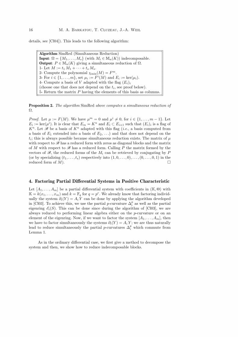
details, see [Cl04]). This leads to the following algorithm:
Algorithm SimRed (Simultaneous Reduction)Input: Ω = M1, . . . ,Ms (with Mi ∈ Mn(K)) indecomposable.Output: P ∈ Mn(K) giving a simultaneous reduction of Ω.1- Let M := t1 M1 + · · ·+ ts Ms.2- Compute the polynomial χmin(M) = Fm.3- For i ∈ 1, . . . ,m, set µi := F i(M) and Ei := ker(µi).4- Compute a basis of V adapted with the flag (Ei)i
(choose one that does not depend on the ti, see proof below).5- Return the matrix P having the elements of this basis as columns.
Proposition 2. The algorithm SimRed above computes a simultaneous reduction ofΩ.
Proof. Let µ := F (M). We have µm = 0 and µi 6= 0, for i ∈ 1, . . . ,m − 1. LetEi := ker(µi). It is clear that Em = Kn and Ei ⊂ Ei+1 such that (Ei)i is a flag ofKn. Let B be a basis of Kn adapted with this flag (i.e., a basis computed froma basis of E1 extended into a basis of E2, . . .) and that does not depend on theti; this is always possible because simultaneous reduction exists. The matrix of µwith respect to B has a reduced form with zeros as diagonal blocks and the matrixof M with respect to B has a reduced form. Calling P the matrix formed by thevectors of B, the reduced forms of the Mi can be retrieved by conjugating by P(or by specializing (t1, . . . , ts) respectively into (1, 0, . . . , 0), . . . , (0, . . . , 0, 1) in thereduced form of M).
4. Factoring Partial Differential Systems in Positive Characteristic
Let [A1, . . . , Am] be a partial differential system with coefficients in (K,Θ) withK = k(x1, . . . , xm) and k = Fq for q = pr. We already know that factoring individ-ually the system ∂i(Y ) = Ai Y can be done by applying the algorithm developedin [Cl03]. To achieve this, we use the partial p-curvature ∆p
i as well as the partialeigenring Ei(S). This can be done since during the algorithm of [Cl03], we arealways reduced to performing linear algebra either on the p-curvature or on anelement of the eigenring. Now, if we want to factor the system [A1, . . . , Am], thenwe have to factor simultaneously the systems ∂i(Y ) = Ai Y ; we are thus naturallylead to reduce simultaneously the partial p-curvatures ∆p
i which commute fromLemma 1.
As in the ordinary differential case, we first give a method to decompose thesystem and then, we show how to reduce indecomposable blocks.

Factoring PDEs in Positive Characteristic 17
4.1. Simultaneous Decomposition
The first step to decompose a partial differential system consists in computing asimultaneous decomposition of the system.
Definition 9. Let [A1, . . . , Am] be a partial differential system with coefficients in(K,Θ). A simultaneous decomposition of [A1, . . . , Am] is given by P ∈ GLn(K)such that:
1. for all i, P [Ai] =
B
[1]i 0
. . .0 B
[d]i
,
2. for all i, the partial p-curvature of each system ∂i(Y ) = B[j]i Y has a charac-
teristic polynomial of the form Fmi,j
i,j with Fi,j irreducible.
Proposition 3. Let [A1, . . . , Am] be a partial differential system with coefficientsin (K,Θ). The matrix P ∈ GLn(K) obtained by applying Algorithm SimDec to∆p
1, . . . ,∆pm provides a simultaneous decomposition of [A1, . . . , Am].
Proof. For any polynomial Q, the spaces ker(Q(∆pi )) are stable under the ∆j
since for all i, j, [∆pi ,∆
pj ] = 0. So P obviously achieves Conditions (i) and (ii) of
Definition 9.
This induces an algorithm for computing a simultaneous decomposition of apartial differential system [A1, . . . , Am]:
• Compute the partial p-curvatures ∆pi of [A1, . . . , Am],
• Return P := SimDec(∆p1, . . . ,∆
pm).
Example 1. Let K := Fp(x1, x2) with p = 3 and consider the D-finite partial dif-ferential system [A1, A2] where A1 and A2 are the following matrices:
A1 =(
1 x1 x2
0 1
),
A2 =
(a(2)1,1
12f2(x2)x2x
41 + 1
2f3(x2)x21 + f4(x2)
− 2f2(x2)x2
f1(x2) + f2(x2)x21
),
where a(2)1,1 = x1−2x3
1x2f2(x2)−f3(x2)x1+x1x2(f1(x2)+f2(x2)x21)
x1x2and f1, f2, f3 and f4 are
functions in the variable x2.
Case 1: first have a look at the case
f1(x2) = x42, f2(x2) = x2, f3(x2) = x6
2, f4(x2) = 2 x62 + 2 x4
2.
Following the algorithm given above, we compute the partial p-curvatures ∆p1
and ∆p2, and then, we apply SimDec to ∆p
1,∆p2: to proceed with the second step,

18 M. A. Barkatou, T. Cluzeau, J.-A. Weil
we form the matrix M = t1 ∆p1 + t2 ∆p
2 and we compute and factor its character-istic polynomial χ(M). We find:
• χ(M)(X) = 2 t2 x152 X+2 t1 t2 x12
2 +2 X t2 x122 +X t2 x3
2+2 t2 x152 t1+t1 t2 x3
2+X2 + 2 X t1 + t1
2 + t22 x18
2 + t22x15
2 + t22x24
2 + 2 t22x27
2 .
The fact that χ(M) is irreducible over K(t1, t2) implies that the partial p-curvatures can not be simultaneously reduced (nor decomposed) and consequently,the partial differential system [A1, A2] is irreducible over K.
Case 2: now, if
f1(x2) = 2 x2, f2(x2) = 0, f3(x2) = 2x62 + x2, f4(x2) = x2 + x2
2.
then, applying the same process, we find:
• χ(M)(X) = (X + t1 + 2 t2 + t2 x32 + t2 x15
2 ) (X + t1 + 2 t2 x32),
so that the system is decomposable.Applying the method of Algorithm SimDec, we find
P :=
(1 2
x2 (x2+x24+x2
10+2 x23x1
2+x211+x2
6+2 x12+x1
2x215)
2 x23+2+x215
0 1
)We can then verify that this matrix decomposes simultaneously the differential sys-tems [A1] and [A2] (and thus the partial differential system):
P [A1] =(
1 00 1
)and
P [A2] =
x26 + 2 x2
2 + 2 x2 + 1x2
0
0 2 x2
.
More generally, we can see that the factorization of the system is the follow-ing:
• If f2(x2) 6= 0, then the system is irreducible,• If f2(x2) = 0, then the system is decomposable.
4.2. Maximal Decomposition
Once a simultaneous decomposition has been computed, we may restrict the studyto each block separately. We are now confronted to the case when the partial differ-ential system [A1, . . . , Am] has partial p-curvatures satisfying χ(∆p
i ) = Fmii with
Fi irreducible and mi ≥ 1. If some mi = 1, then [A1, . . . , Am] is irreducible andthe factorization stops.

Factoring PDEs in Positive Characteristic 19
Let M denote the (partial) differential module associated with the system[A1, . . . , Am]. We want to find a maximal decomposition of M , i.e., a decomposition
M = W1 ⊕ · · · ⊕Wd,
where the Wi are indecomposable. As a result, we will write the differential system[A1, . . . , Am] in block diagonal form where the modules corresponding to the di-agonal blocks are indecomposable. Here, the techniques from the previous sectiondo not apply because a matrix P ∈ GLn(K) that decomposes simultaneously the∆p
i does not necessarily decompose the differential systems ∂i(Y ) = Ai Y .
To handle this case, we can use the eigenring. In [Cl03, Proposition 4.7], it isshown that there exists a ”separating” element in the eigenring. This is a matrixT with characteristic polynomial χ(T ) = F1 · · ·Fd such that gcd(Fi, Fj) = 1 andχ(T|Wi
) = Fi. Applying a classical result of the eigenring factorization method (see[Ba01, Theorem 2] or [Cl04, Proposition 6]) to this element T yields a maximaldecomposition of M .
In practice, such a separating element can be found by taking random ele-ments in the eigenring. In case of failure, one can use the idempotent decompositionof the eigenring from [GZ03] to obtain a maximal decomposition.
As noted in [Cl03], one can also adapt here the method proposed by van derPut in [Pu97, PS03]. Let ai denote a root of Fi, i.e., the image of X in K[X]/(F ).Let K+ := K(a1, . . . , am). Applying the algorithm of Subsection 4.1 over K+, weare reduced to studying a differential module M + over K+ having p-curvatureswith characteristic polynomial of the form (X − ai)mi . The latter can be reduced(over K+) using Subsection 2.3 and, thus, we obtain a differential module M +
(over K+) with a maximal decomposition (and a complete reduction of the inde-composable blocks). Now, K+ has a structure of differential module over K andwe have M = M + ⊗K K+: from this, we recover a basis of M over K and, then,a maximal decomposition of M (and the indecomposable blocks are fully reduced).
This last method can turn out to be costly because it may require to work inan unnecessary algebraic extension. In the next section, we give a simple rationalalternative to handle the reduction of indecomposable partial differential systems.
4.3. Reducing Indecomposable Blocks
Definition 10. Let [A1, . . . , Am] be an indecomposable partial differential systemwith coefficients in (K,Θ). A (maximal) simultaneous reduction of [A1, . . . , Am]is given by an invertible matrix P such that:

20 M. A. Barkatou, T. Cluzeau, J.-A. Weil
1. for all i, P [Ai] =
B
[1]i ∗ . . . ∗
0 B[2]i
. . ....
.... . . . . . ∗
0 . . . 0 B[r]i
,
2. for all i, the partial p-curvature of each system ∂i(Y ) = B[j]i Y has a minimal
polynomial of the form Fi with Fi irreducible.
Proposition 4. Let S = [A1, . . . , Am] be an indecomposable partial differential sys-tem with coefficients in (K,Θ). The matrix P ∈ GLn(K) obtained by applying Algo-rithm SimRed to ∆p
1, . . . ,∆pm provides a simultaneous reduction of [A1, . . . , Am].
Proof. In the proof of Proposition 2, we have constructed an element µ and aninvertible matrix P such that P−1 µP = S where S is block triangular withzeros as diagonal blocks. Now, we remark that, after turning (t1, . . . , ts) into some(0, . . . , 0, 1, 0, . . . , 0) (the 1 is in the i-th position) the element µ[i] obtained is anon-zero and non-invertible element in the partial eigenring Ei(S). Then, for thesame reasons as in the proof of [Ba01, Theorem 1], a direct calculation showsthat, Bi := P [Ai] has a reduced form (compare to the proof of [Cl03, Proposition5.1]).
We obtain thus the following method to compute a simultaneous reductionof indecomposable partial differential systems.• Compute the partial p-curvatures ∆p
i of [A1, . . . , Am],• Return P := SimRed(∆p
1, . . . ,∆pm).
5. Two Other Generalizations
We have shown in the previous sections 3 and 4 how to generalize the algorithm of[Cl03] to factor partial differential systems in characteristic p. We will now see thatthis algorithm can be directly adapted to other situations as well. We will sketchthe algorithms corresponding to [Cl03] in the case of one variable but, followingthe approach of Sections 3 and 4 to generalize [Cl03] to the multivariate case,one would obtain algorithms for factoring (integrable) partial local systems and(integrable) partial difference systems.
5.1. “Local” Factorizations
In this subsection, we give the elements needed to generalize the algorithm factor-ing differential systems with coefficients in K = k(x) with k = Fq for some q = pr
to the case where the coefficients belong to K((x)).
Let [A] be a differential system with A ∈ Mn(K((x))). The notions of p-curvature and eigenring can be defined as in the ordinary differential case. Notingthat K((x)) is a C1-field ([Ja80, Definition 11.5, p.649]), we deduce that the clas-sification of differential modules in characteristic p given by van der Put in [Pu95]
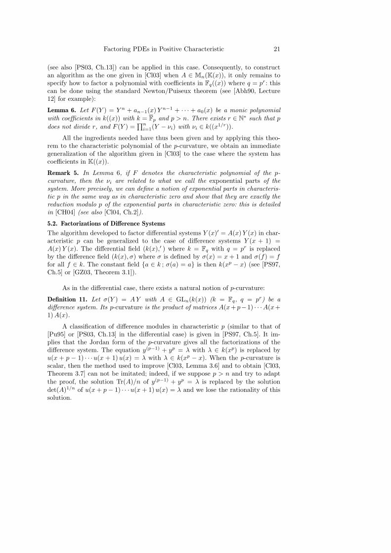
Factoring PDEs in Positive Characteristic 21
(see also [PS03, Ch.13]) can be applied in this case. Consequently, to constructan algorithm as the one given in [Cl03] when A ∈ Mn(K(x)), it only remains tospecify how to factor a polynomial with coefficients in Fq((x)) where q = pr: thiscan be done using the standard Newton/Puiseux theorem (see [Abh90, Lecture12] for example):
Lemma 6. Let F (Y ) = Y n + an−1(x) Y n−1 + · · · + a0(x) be a monic polynomialwith coefficients in k((x)) with k = Fp and p > n. There exists r ∈ N∗ such that p
does not divide r, and F (Y ) =∏n
i=1(Y − νi) with νi ∈ k((x1/r)).
All the ingredients needed have thus been given and by applying this theo-rem to the characteristic polynomial of the p-curvature, we obtain an immediategeneralization of the algorithm given in [Cl03] to the case where the system hascoefficients in K((x)).
Remark 5. In Lemma 6, if F denotes the characteristic polynomial of the p-curvature, then the νi are related to what we call the exponential parts of thesystem. More precisely, we can define a notion of exponential parts in characteris-tic p in the same way as in characteristic zero and show that they are exactly thereduction modulo p of the exponential parts in characteristic zero: this is detailedin [CH04] (see also [Cl04, Ch.2]).
5.2. Factorizations of Difference Systems
The algorithm developed to factor differential systems Y (x)′ = A(x) Y (x) in char-acteristic p can be generalized to the case of difference systems Y (x + 1) =A(x) Y (x). The differential field (k(x),′ ) where k = Fq with q = pr is replacedby the difference field (k(x), σ) where σ is defined by σ(x) = x + 1 and σ(f) = ffor all f ∈ k. The constant field a ∈ k ; σ(a) = a is then k(xp − x) (see [PS97,Ch.5] or [GZ03, Theorem 3.1]).
As in the differential case, there exists a natural notion of p-curvature:
Definition 11. Let σ(Y ) = A Y with A ∈ GLn(k(x)) (k = Fq, q = pr) be adifference system. Its p-curvature is the product of matrices A(x+p−1) · · ·A(x+1) A(x).
A classification of difference modules in characteristic p (similar to that of[Pu95] or [PS03, Ch.13] in the differential case) is given in [PS97, Ch.5]. It im-plies that the Jordan form of the p-curvature gives all the factorizations of thedifference system. The equation y(p−1) + yp = λ with λ ∈ k(xp) is replaced byu(x + p − 1) · · ·u(x + 1)u(x) = λ with λ ∈ k(xp − x). When the p-curvature isscalar, then the method used to improve [Cl03, Lemma 3.6] and to obtain [Cl03,Theorem 3.7] can not be imitated; indeed, if we suppose p > n and try to adaptthe proof, the solution Tr(A)/n of y(p−1) + yp = λ is replaced by the solutiondet(A)1/n of u(x + p− 1) · · ·u(x + 1)u(x) = λ and we lose the rationality of thissolution.

22 M. A. Barkatou, T. Cluzeau, J.-A. Weil
One can define an eigenring as well (see for example [Ba01, GZ03]): let σ(Y ) =A Y be a difference system with A ∈ Mn(k(x)). The eigenring E(A) of [A] is theset defined by
E(A) = P ∈ Mn(k(x)) |σ(P )A = A P.
All the elements needed to develop an algorithm similar to that of [Cl03] arecollected and the algorithm follows naturally. Note further that:• The results of [Ba01] stay true in the difference case ([Ba01] is written in the
general setting of pseudo-linear equations),• The algorithm of Giesbrecht and Zhang ([GZ03]) can be used to factor Ore
polynomials thus, in particular, difference operators.
Acknowledgments: the authors would like to thank Alban Quadrat for helpfulexplanations and references concerning D-finite partial differential systems andJanet bases, and Marius van der Put for his comments and the appendix thatfollows.
References
[Abh90] S. S. Abhyankar. Algebraic geometry for scientists and engineers. Mathemat-ical Surveys and monographs, number 35. Published by the A.M.S., 1990.
[Ba01] M. A. Barkatou. On the reduction of matrix pseudo-linear equations. Tech-nical Report RR 1040, Rapport de Recherche de l’institut IMAG, 2001.
[BP99] M. A. Barkatou and E. Pflugel. An algorithm computing the regular singu-lar formal solutions of a linear differential system. In Journal of SymbolicComputation 28(4-5), 1999.
[BCGPR03] Y. A. Blinkov, C. F. Cid, V. T. Gerdt, W. Plesken and D. Robertz.The Maple package “Janet”: II. Polynomial Systems. In Proceedingsof Computer Algebra and Scientific Computing (CASC), Passau, 2003.http://wwwmayr.informatik.tu-muenchen.de/CASC2003/
[CO68] L. Chambadal and J. L. Ovaert. Algebre lineaire et algebre tensorielle. DunotUniversite, Paris, 1968.
[Ch01] A. Chambert-Loir. Theoremes d’algebricite en geometrie diophantienne.Seminaire Bourbaki, expose No. 886, Mars 2001.
[Cl03] T. Cluzeau. Factorization of differential systems in characteristic p. In Pro-ceedings of ISSAC’03, ACM Press, 58-65, 2003.
[Cl04] T. Cluzeau. Algorithmique modulaire des equations differentielles lineaires.These de l’universite de Limoges, Septembre 2004.
[CH04] T. Cluzeau and M. van Hoeij. A modular algorithm for computing the ex-ponential solutions of a linear differential operator. In Journal of SymbolicComputation, 38(3): 1043-1076, 2004.
[CGT97 ] R. Corless,P. Gianni, B. Trager. A reordered Schur factorization method forzero-dimensional polynomial systems with multiple roots. In Proceedings of

Factoring PDEs in Positive Characteristic 23
the 1997 International Symposium on Symbolic and Algebraic Computation,133-140 ACM, New York, 1997.
[GZ03] M. Giesbrecht and Y. Zhang. Factoring and decomposing Ore polynomialsover Fp(t). In Proceedings of ISSAC’03, ACM Press, 127-134, 2003.
[HS02] M. Hausdorf and M. Seiler. Involutives basis in MuPAD-Part I: involutivedivisions. In MathPad, 11/1: 51-56, 2002.
[HRUW98] M. van Hoeij, J.-F. Ragot, F. Ulmer and J.-A. Weil. Liouvillian solutions oflinear differential equations of order three and higher. In Journal of SymbolicComputation, 11: 1-17, 1998.
[Ja53] N. Jacobson. Lectures in abstract algebra. II. Linear algebra. Graduate Textsin Mathematics 31, Springer-Verlag, 1953.
[Ja80] N. Jacobson. Basic algebra II. W.H. Freeman and Compagny, San Francisco,1980.
[Ja20] M. Janet. Sur les systemes aux derivees partielles. In Journal de Math., 8-emeserie, III, 65-151, 1924.
[Ja29] M. Janet. Lecons sur les systemes d’equations aux derivees partielles. CahiersScientifiques, IV, Gauthiers-Villars, 1929.
[Ka70] N. Katz. Nilpotent connections and the monodromy theorem: applications ofa result of Turritin. Publ. Math. I. H. E. S., 39: 355-412, 1970.
[Ka82] N. Katz. A conjecture in the arithmetic theory of differential equations. Bull.Soc. Math. France, 110: 203-239, 1982.
[Le94] A. H. M. Levelt. The semi-simple part of a matrix. In Algorithmen in de Al-gebra, 85-88, 1994. http://www.math.ru.nl/medewerkers/ahml/other.htm
[LST02] Z. Li, F. Schwarz and S. P. Tsarev. Factoring zero-dimensional ideals of linearpartial differential operators. In Proceedings of ISSAC’02, ACM Press, 168-175, 2002.
[LST03] Z. Li, F. Schwarz and S. P. Tsarev. Factoring systems of linear PDEs withfinite-dimensional solution spaces. Journal of Symbolic Computation, 36(3-4):443-471, 2003.
[Pu95] M. van der Put. Differential equations in characteristic p. Compositio Math.,97: 227-251, 1995.
[Pu97] M. van der Put. Modular methods for factoring differential operators. Man-uscript, 1997.
[PS97] M. van der Put and M. F. Singer. Galois theory of difference equations. Lec-tures Notes in Mathematics, vol. 1666, Springer (Berlin), 1997.
[PS03] M. van der Put and M. F. Singer. Galois Theory of Linear Differential Equa-tions Grundlehren der mathematischen Wissenschaften, vol. 328, Springer,2003.
[Si96] M. F. Singer. Testing reducibility of linear differential operators: a grouptheoretic perspective. Journal of Appl. Alg. in Eng. Comm. and Comp., 7(2):77-104, 1996.
[Wu05] M. Wu. Factoring Finite-Dimensional Differential Modules. This volume.

24 M. A. Barkatou, T. Cluzeau, J.-A. Weil
Appendix: Classification of Partial Differential Modules in PositiveCharacteristic.
By Marius van der Put,University of Groningen, Department of MathematicsP.O. Box 800, 9700 AV Groningen, The Netherlands
(1) Introduction. In [Pu95, PS03] a classification of differential (resp. differ-ence in [PS97]) modules over a differential field K of characteristic p > 0 with[K : Kp] = p is given. The differential modules in question can be seen as ordi-nary matrix differential equations. Here we show how to extend this to, say, thecase [K : Kp] = pm with m > 1 (compare [1], 6.6 Remarks (1)). The (partial)differential modules are the partial differential equations considered in this paper.In order to simplify the situation, we will, as in the paper, avoid the skew fieldthat may arise in the classification. The algorithmic results of the paper are mademore transparent from the classification that we will work out.
(2) Assumptions and notation. Let K be a field of characteristic p > 0 andlet K0 be a subfield such that the universal differential module ΩK/K0 has dimen-sion m ≥ 1 over K. There are elements x1, . . . , xm ∈ K such that dx1, . . . , dxmis a basis of ΩK/K0 . Then x1, . . . , xm form a p-basis of K/K0 which means thatthe set of monomials xa1
1 · · ·xamm |0 ≤ ai < p for all i is a basis of K over
KpK0. We will write C := KpK0. For i ∈ 1, . . . ,m, the derivation ∂i of K/K0
is given by ∂ixj = δi,j . Clearly, the ∂i is a set of commuting operators. PutD := K[∂1, . . . , ∂m]. This is a ring of differential operators and the partial differ-ential equations that one considers (in the paper and here) are left D-modules Mof finite dimension over K. We note that M is a cyclic module (and thus M ∼= D/Jfor some left ideal J of finite codimension) if dimK M ≤ p. If dimK M > p, thenin general M is not cyclic (compare [2], Exercise 13.3, p. 319). For notational con-venience we will write D-module for left D-module of finite dimension over K.
(3) Classification of the irreducible D-modules.Similarly to [Pu95], one can prove the following statements. The center Z of D isC[t1, . . . , tm]. The latter is a (free) polynomial ring in the variables ti := ∂p
i mi=1.
Consider any maximal ideal m ⊂ Z and put L = Z/m. Then L ⊗Z D is a cen-tral simple algebra over L of dimension p2m. The well known classification impliesthat this algebra is isomorphic to a matrix algebra Matr(pm1 , D) where D is a(skew) field having dimension p2m2 over its center L. Clearly m1 + m2 = m.The unique simple left module M of this algebra is Dpm1 and has dimensionp−m[L : C]pm1+2m2 = pm2 [L : C] over K. In particular, if the dimension of Mover K is < p, then L⊗Z D is isomorphic to Matr(pm, L).

Factoring PDEs in Positive Characteristic 25
Let M be an irreducible D-module. Then M is also a Z-module of finitedimension over C. The irreducibility of M implies that mM = 0 for some maxi-mal ideal m of Z (write again L = Z/m). Hence M is a simple left module overL⊗Z D. If one knows the structure of the algebras L⊗Z D, then the classificationof irreducible D-modules is complete.
(4) Isotypical decomposition.Let M be any D-module. Put I := a ∈ Z | aM = 0, the annulator of M . ThenI ⊂ Z is an ideal of finite codimension. Thus M is also an Z/I-module of finitedimension. Let m1, . . . ,ms denote the set of maximal ideals containing I. This isthe support of M . Then the Artin ring Z/I is the direct product of the local Artinrings Zmi
/(I). One writes 1 = e1+· · ·+em, where ei is the unit element of the ringZmi
/(I). Then M = ⊕Mi, with Mi = eiM . This is a module over Zmi/(I). Since
Z is the center of D each Mi is again a D-module. Moreover, the annulator of Mi
is an ideal with radical mi. The above decomposition will be called the isotypicaldecomposition of M . The classification of D-modules is in this way reduced to theclassification of D-modules with are annihilated by a power of some maximal idealm of Z. The latter depends on the structure of Z/m⊗Z D.
(5) Restricting the class of D-modules.Let S denote the set of maximal ideals s = m in Z such that the algebra Z/m⊗ZDis isomorphic to Matr(pm, Z/m). In the sequel we will only consider D-moduleswith support in S. The differential modules M , considered in this paper, satisfydimK M < p. According to (3), their support is in S. We note that S depends onthe fields K0 ⊂ K. There are examples where S is the set of all maximal ideals of Z.
(6) Classification of the D-modules with support in s, where s ∈ S.We fix a maximal ideal s = m ∈ S. The above Tannakian category will be denotedby (D, s). We note that the tensor product M1⊗M2 of two object in this categoryis defined as M1 ⊗K M2, provided with the action of ∂i (for i = 1, . . . ,m) givenby ∂i(m1 ⊗m2) = (∂im1)⊗m2 + m1 ⊗ (∂im2).
Consider the category (Z, s) of the finitely generated Z-modules N , withsupport in s. The Tannakian structure of this category is determined by thedefinition of a tensor product. The tensor product of two modules N1, N2 in (Z, s)is N1 ⊗C N2 equipped with the operations ti given by ti(n1 ⊗ n2) = (tin1)⊗ n2 +n1 ⊗ (tin2).
The aim is to produce an equivalence Fs : (Z, s) → (D, s) of Tannakian cate-gories. Once this is established, the required classification is reduced to classifyingthe objects of (Z, s). The functor Fs is defined as Fs(N) = M := K ⊗C N . Theright hand side is clearly a (left) K[t1, . . . , tm]-module. It suffices to extend this toa left D-module by defining the operation of the ∂i on M .

26 M. A. Barkatou, T. Cluzeau, J.-A. Weil
Let Zs denote the completion of the local ring Zm. Let (Zs, s) denote thecategory of the Zs-modules of finite dimension over C. The categories (Z, s) and(Zs, s) are clearly the ‘same’. Put Ds = Zs⊗ZD and let (Ds, s) denote the categoryof the left Ds-modules which have finite dimension over K. Then the categories(D, s) and (Ds, s) are the ‘same’. Therefore it suffices to construct an equivalenceFs : (Z, s) → (Ds, s).
For this purpose we need a free, rank one, Zs⊗C K-module Qs = Zs⊗C Ke,such that its structure of Zs ⊗C K-module extends to that of a left Ds-module.Given Qs, the functor Fs is defined by N 7→ M := N ⊗bZs
Qs. Then M is aleft Ds-module by λ(n ⊗ µe) = n ⊗ (λµ)e. It is easily verified that Fs is indeedan equivalence of Tannakian categories. We note that M is equal to N ⊗C K asZs⊗C K-module, and our construction extends this to a left Ds-module structure.
(7) The construction of Qs.By assumption A0 := Z/m ⊗Z D is isomorphic to Matr(pm, Z/m). Let I be the(unique) simple left module of A0. Then the morphism A0 → EndZ/m(I) is a bi-jection. In particular, the commutative subalgebra Z/m⊗C K of A0 acts faithfullyon I. By counting dimensions over C, one sees that I is in fact a free Z/m⊗C K-module with generator, say, e. Thus we have found a left A0-module structure onZ/m ⊗C Ke. Now Qs is constructed by lifting this structure, step by step, to aleft Ds-module structure on Zs ⊗C Ke. This is in fact equivalent to lifting a givenisomorphism A0 → Matr(pm, Z/m) to an isomorphism Qs → Matr(pm, Zs). Themethod of [1] for the case m = 1, can be extended here. For notational conveniencewe present here a proof for the case p = 2 and m = 2.
We note that Zs ⊗C K = Zs[x1, x2] has a free basis 1, x1, x2, x1x2 overZs. Consider the free module Zs[x1, x2]e. We have to construct operators ∂1 and∂2 on this module such that ∂1∂2 − ∂2∂1 = 0 and ∂2
i = ti for i = 1, 2. Put∂ie = `ie for i = 1, 2. Then the conditions are ∂i(`i) + `2i − ti = 0 for i = 1, 2 and∂1(`2) − ∂2(`1) = 0. Suppose that we have found `1, `2 such that these equalitieshold modulo ms. Then we want to change the `i in `i+ri with r1, r2 = 0 mod (ms)such that the required equalities hold module ms+1. This step suffices for the proofof the statement. It amounts to solving
∂i(ri) = −∂(`i)− `2i + ti mod ms+1 and
∂1(r2)− ∂2(r1) = ∂2(`1)− ∂1(`2) mod ms+1.
The right hand sides of the equalities are already 0 mod ms. Write r1 = r1(0, 0)+r1(1, 0)x1 + r1(0, 1)x2 + r1(1, 1)x1x2 and similarly for r2. The right hand side ofthe first equation with i = 1, is killed by the operator ∂1 and therefore containsonly the terms 1, x2. This leads to a unique determination of r1(1, 0) and r1(1, 1)and the r1(0, 0), r1(0, 1) can be chosen freely. Similarly, the terms r2(0, 1), r2(1, 1)

Factoring PDEs in Positive Characteristic 27
are determined and the terms r2(0, 0), r2(1, 0) can be chosen freely. The secondequation reads
r2(1, 0)− r1(0, 1) + r2(1, 1)x2 − r1(1, 1)x1 = ∂2(`1)− ∂1(`2) mod ms+1.
The right hand side R uses only the terms 1, x1, x2. Moreover, ∂1(R) = ∂1∂2(`1) =∂2∂1(`1) and this is equal to ∂2(∂1(`1)+ `21− t1). Hence the coefficients of x1 of thetwo sides are equal. The same holds for the coefficients of x2. The coefficient of1 on the two sides can be made equal for a suitable choice of r1(0, 1) and/or r2(1, 0).
(8) Final remarks.Let (Z, S) denote the Tannakian category of the Z-modules, having finite di-mension over C and with support in S. Let (D, S) denote the category of theleft D-modules having finite dimension over K and with support in S (as Z-module). One can ‘add’ the equivalences Fs in an obvious way to an equivalenceF : (Z, S) → (D, S). For an object M of (D, S), there is an object N of (Z, S)such that F(N) = M . Then M , as module over K[t1, . . . , tm], describes in fact thep-curvature of M . Since N ⊗C K ∼= M , one can say that N represents already thep-curvature of M . In particular, the characteristic (and minimal) polynomials forthe ti have their coefficients in C = K0K
p.
As observed before, classifying the left D-modules of finite dimension overK and with support in S is equivalent to classifying the Z-modules of finitedimension over C and with support in S. The latter is done by decomposingan object into isotypical components. Hence we may restrict our attention toa single maximal ideal s = m ∈ S. The modules N that we want to classifyare in fact the finitely generated modules over the complete regular local ringZs
∼= L[[d1, . . . , dm]] which are annihilated by a power of the maximal ideal m. Un-like the case m = 1, no reasonable classification (or moduli spaces) seems possible.One observation can still be made. The module N has a sequence of submodules0 = N0 ⊂ N1 ⊂ · · · ⊂ Nt = N such that each quotient Ni+1/Ni is isomorphic tothe module L = Z/m. In other words, N is a multiple extension of the module L.
——–
M. A. Barkatou, T. Cluzeau, J.-A. WeilLACO, Universite de Limoges123 avenue Albert Thomas87060 Limoges, Francee-mail: moulay.barkatou,thomas.cluzeau,[email protected]