Policy Research Working Paper 8070

Fuel Efficiency Versus Fuel Substitution in the Transport Sector

An Econometric Analysis

Gal HochmanGovinda R. Timilsina

Development Research GroupEnvironment and Energy TeamMay 2017

WPS8070P

ublic

Dis

clos

ure

Aut

horiz

edP

ublic

Dis

clos

ure

Aut

horiz

edP

ublic

Dis

clos

ure

Aut

horiz

edP

ublic

Dis

clos

ure

Aut

horiz

ed

Produced by the Research Support Team

Abstract

The Policy Research Working Paper Series disseminates the findings of work in progress to encourage the exchange of ideas about development issues. An objective of the series is to get the findings out quickly, even if the presentations are less than fully polished. The papers carry the names of the authors and should be cited accordingly. The findings, interpretations, and conclusions expressed in this paper are entirely those of the authors. They do not necessarily represent the views of the International Bank for Reconstruction and Development/World Bank and its affiliated organizations, or those of the Executive Directors of the World Bank or the governments they represent.

Policy Research Working Paper 8070

This paper is a product of the Environment and Energy Team, Development Research Group. It is part of a larger effort by the World Bank to provide open access to its research and make a contribution to development policy discussions around the world. Policy Research Working Papers are also posted on the Web at http://econ.worldbank.org. The authors may be contacted atgtimilsina@worldbank.org.

The transport sector offers limited options to reduce green-house gas emissions as compared with other sectors, such as power generation and industrial sectors. To understand the potential reduction of energy consumption and associated emissions through fuel substitution or transportation service demand reduction, this study estimates own- and cross-price elasticities of various fuels used for transportation. The

analysis shows, like many previous studies, that an increase in fuel prices would not have a large effect on transport sector carbon dioxide emissions, due to limited substitution possibilities among fuels for transportation. The study also finds that price-induced changes that lead to an increase in the rate of adoption of fuel-efficient vehicles would be more effective than a policy to cause fuel substitution.

Fuel Efficiency Versus Fuel Substitution in the Transport Sector:

An Econometric Analysis*

Gal Hochman and Govinda R. Timilsina†

Keywords: emission intensity, fuel switching, cross-price elasticity, own-price elasticity,

transportation sector

JEL Code: Q4

* The authors would like to thank Scholastica Okoye for research assistantship, and Jon Strand, Sam Asher and MikeToman for their valuable comments and suggestions. The views and interpretations are of authors and should not beattributed to the World Bank Group. Financial support from the Knowledge for Change (KCP) Trust Fund of theWorld Bank is acknowledged.

† Gal Hoachman (gal.hochman@rutgers.edu) is an Associate Professor at Department of Economics, Rutgers University, New Jersey and Govinda Timilsina (gtimilsina@worldbank.org) is a Senior Economist, Development Research Group, World Bank; Washington, DC

2

1. Introduction

Fossil fuels are the main anthropogenic source of greenhouse gas (GHG) emissions, and the

transportation sector (including international aviation and marine transportation) contributes

almost one-fourth of the current global GHG emissions from energy consumption and production

activities (IEA, 2016b). More than 90% of the world’s transportation fuels is supplied by

petroleum-based sources (IEA, 2016a). Unlike other sectors, such as power generation and

industry, opportunities to substitute petroleum with other fuels are more limited in the

transportation sector. The lower fuel substitution possibility leaves fewer options to respond to a

fuel price increase: reducing demand in the short-run and adopting more energy efficient vehicles

(i.e., vehicles that give higher kilometers per liter of fuel use) in the long-run. The latter is an

outcome of technological change (Gales et al., 2007; Liao et al., 2007; Ma & Stern, 2008; Metcalf,

2008).

In the long-run, drivers could also exercise fuel substitution potential through vehicle switching,

for example, replacing gasoline-driven vehicles with diesel-driven vehicles if transport cost with

diesel is lower as compared to that of gasoline. They can also use public transportation (bus, train)

instead of driving cars. Some substitution of gasoline vehicles with compressed natural gas (CNG)

vehicles has occurred in many countries, including developing countries, such as India, Pakistan

and Bangladesh (Timilsina and Shrestha, 2009). However, the analysis of this paper suggests that

the substitution of gasoline-driven vehicles with CNG-driven ones is mainly caused by policies

(e.g., government mandates in India, heavy subsidies to natural gas in Pakistan and Bangladesh)

rather than market forces.

3

The substitution possibilities among fuels is the key driver to a successful implementation

of market-based policy instruments in reducing GHG emissions from the transportation sector.

This is because the higher are substitution possibilities among the transportation fuels, the larger

would be the efficacy of market-based instruments. The substitution possibilities between fuels or

between modes of transportation can be measured in terms of elasticity of substitutions. In

addition, by comparing estimates of partial elasticities of substitution (a measure of fuel switching)

with that of total elasticities of substitution (a measure of both fuel switching as well as changes

in total fuel use), the importance of alternative market mediated policies can be evaluated. The

benefits of a policy that affects the relative prices of fuels, and thus drives fuel-switching, can be

compared with those of a policy that promotes fuel-efficiency.

Several existing studies have focused on estimating price elasticity of transportation fuels,

particularly gasoline. For example, studies such as Dahl and Sterner (1991), Dahl (2012), Espey

(1998), Kayser (2000) and Holmgren (2007) estimated that the short-run own-price elasticity of

gasoline spans a range between -0.08 and -0.54. Other studies, such as Burke and Nishitateno

(2013), estimated the long-run own-price elasticity of gasoline to vary between −0.2 and −0.5.

Existing studies have also compared the long-run elasticity of car travel with long-run own-price

elasticity and reported the former is lower than the latter because of increase in fuel efficiency.3

For example, Dargay (2007) finds that the elasticity of car travel to fuel prices in the long-run was

3 The average miles per gallon of the light-duty vehicle fleet in the United States increased from 14.9 miles in 1980

to 20 miles in 2020 and further to 21.4 miles in 2014. Similarly, the average miles per gallon of the new light-duty

vehicle fleet increased from 24.3 miles in 1980 to 28.5 miles in 2000 and further to 36.4 miles in 2014 (US Bureau

of Transportation Statics,

https://www.rita.dot.gov/bts/sites/rita.dot.gov.bts/files/publications/national_transportation_statistics/html/table_04_

23.html).

4

only -0.14, which is lower in magnitude as compared to the lowest magnitude of long-run own

price elasticity of gasoline reported by the literature. There also exist some studies that estimate

both own-price elasticities and cross-price elasticities of fuels used in the transport sector. For

example, Serletis et al. (2010) estimate own and cross price elasticities of four fuels, fuel oil,

electricity, gasoline and diesel, using data from selected OECD countries.

The main objective of our study is to compare two specific policies in the transport sector,

fuel efficiency improvement and fuel switching, to reduce GHG emissions. To do this, we estimate

own and cross price elasticities for various OECD countries. For this purpose, we used a translog

cost function, which is widely used in the literature (see e.g., Berndt & Woods,1975; Fuss, 1977;

Griffin, 1977; Pindyck, 1979; Uri, 1979; Hall, 1986) for the estimation. First, we hold the total

demand for fuel in the road transportation sector constant and calculate the Allen partial elasticities

of substitution (Uzawa, 1962). We then use these Allen partial elasticities to calculate the partial

own- and cross-price elasticities of the various fuels in different OECD countries. In the second

step, we relax the assumption that total demand for fuel in the road transportation sector is constant,

and estimate total own- and cross-price elasticities. While the estimated values of partial cross-

price elasticity measure fuel switching possibilities, the differences between partial and total own-

price elasticities estimate the effect of fuel efficiency improvements and the reduction in energy

consumption in the transportation sector.

Some existing literature (Greening et al. 1999; Greening, 2004; Lu et al. 2007; Paravantis

and Georgakellos, 2007; Timilsina and Shrestha, 2008 and Timilsina and Shrestha, 2009) has used

the identity approach to compare the roles of various factors, such as change in fuel mix, improved

fuel efficiency, change in transportation modes, etc. in influencing the historical trends of transport

sector energy consumption or CO2 emissions from this sector. Although the identity approach has

5

been widely used to investigate national and sectoral energy and emission intensities (Ang and

Zhang, 2000), it simply examines trends and does not use statistical techniques to establish the

relationship between the changes in energy or emission intensities and the factors that might have

caused the changes. Second, the approach does not account for changes in fuel prices and their

potential roles on the changes in energy consumption and corresponding emissions.

The results from our study suggest that alternative mode of transportation, including the

electrification of vehicle fleets, have not reached the threshold where the population at large is

willing to adopt these alternative technologies to the internal combustion engine. Thus, improving

fuel efficiency and increasing distance per unit of fuel use of current transportation modes has

major implications for the emissions generated by the transportation sector in the short to medium

run. The study presents a new way to represent fuel efficiency improvement through own price

elasticities, and to compare, using estimated values of elasticities of transportation fuels, the key

policy instruments to reduce GHG emissions from the transport sector. Moreover, the estimated

values of own and cross price elasticities using a long time series of data from all OECD countries

can be used in models for energy demand forecasts in the transport sector and economy-wide, as

well as in sectoral models, to assess impacts of climate change mitigation policies.

The paper is organized as follows. Section 2 of this study describes the empirical

framework used to estimate the partial (total) own- and cross-price elasticities. The data utilized

are presented in section 3. In section 4, the own- and cross-price elasticity estimates are presented

and the policy implications of the results are discussed. We offer policy discussion and concluding

remarks in section 5.

6

2. Methodology

We developed an empirical model to estimate the responsiveness of various fuels in the

transportation sector to changes in price. Following Fuss (1977) and Pindyck (1979), we start with

a model that employs a translog cost function that is homothetically separable in its inputs (a

similar framework is employed in Berndt and Woods (1975), Griffin (1977), Uri (1979), and Hall,

(1986)). Because the translog cost function is homotehtically separable, we can focus only on the

energy input in the transportation sector, estimate the sensitivity to changes in prices, and better

understand the effect of prices on fuel switching.

Technically, assume transportation services from different modes (e.g., road, rail, air,

water) are produced using energy/fuels (F) as well as non-energy inputs (i.e., capital (K), labor

(L), and materials (M)). 4 Let F denote the set of the different types of fuels used in the

transportation sector; that is,

∈ ≡ gasoline, diesel, natural gas, LPG, electricity

We restrict the structure of production as follows:

Assumption 1: The production function is weakly separable in its aggregate inputs.

Assumption 1 suggests that the marginal rates of substitution between the various fuels

used in the transportation sector are independent of other aggregate inputs (capital, labor, and

materials). This assumption leads to aggregate energy price indexes for the transport sector. To

4 Capital costs include rental value of vehicles, labor costs are the driver’s costs, and materials are operation and

maintenance costs.

7

this end, Halvorsen and Ford (1978) used translog cost functions and tested the separability of

energy from other inputs, focusing on the individual two-digit industries in the United States. They

found that the separability holds for four of the eight industries in the United States.

Assumption 2: Energy aggregates are homothetic in the various components.

Assumption 2 suggests a two-step optimization process that results in the model’s solution.

In the first step, the optimal fuel mix that yields the energy input is derived, and then input use is

optimized across the various aggregate inputs (energy, capital, labor, and materials).

Assumptions 1 and 2, then, suggest the following aggregate country-level transportation

production function:

= ∈ , , ,

where T(.) is a homothetic function of the F fuels, and H(.) is a smooth function. Given the

production structure assumed, the study henceforth focuses on the function T(.).

Assume that firms take prices as given and let PE denote the aggregate price index of energy

used for transportation, which is homothetic and not a function of quantity. Let small letters denote

the log of the variable, pf denotes the log of price of fuel f, ∈ , c denotes the log of cost function,

and define the share equations as = ⁄ . Then, the steps employed in estimating the

parameters used to calculate the various elasticities and the transportation energy price index are

as follows:

1) First, we estimated the fuel shares: = + ∑ ,∈ for , ∈ (1)

8

We estimated Eq. (1) assuming the following restrictions (which are the outcome of

Assumptions 1 and 2):

(a) , = ,

(b) ∑ ∈ = 1

(c) ∑ ,∈ = ∑ ,∈ = 0

2) Next, we used the estimated parameters and , for , ∈ to calculate the

aggregate energy price indexes of the transportation sector for the various countries. To

calculate the aggregate energy-price indexes, the following equation was employed: = + ∑ ∈ + ∑ ∑ ,∈∈ (2)

When calculating Eq. (2), we normalized such that the aggregate energy price index for

the United States in 2010 is 1.

The parameters estimated in step (1) are, then, used to estimate the partial own- and cross-

elasticities. To this end, we first calculate the Allen partial elasticities and then use these estimates

to calculate the partial elasticities of interest. Following Uzawa (1962), when calculating the Allen

partial elasticities of substitution, the translog cost function suggests the following:

= + for ≠ , (3)

= + 1 −

Then, the partial own- and cross-price elasticities of demand, respectively, are

= ; = for ≠ , (4)

These are partial price elasticities that only account for substitution among fuels assuming that

total energy consumed by the transportation sector is constant.

9

When allowing total energy to change with changes in fuel price, the responsiveness of

quantities to a given price change is much larger. The total elasticity is defined as

= + (5)

That is, total elasticity is the sum of the partial elasticity plus ‒ called the cost

effect, which is the outcome and change in amount of energy consumed. The empirical analysis

suggests that the cost effect is important in the transportation sector; that is, the use of policy to

increase fuel efficiency in the transportation sector is likely to reduce GHGs (measured through

pricing effect within a given fuel) and this effect is of similar magnitude to that of policy that

promotes wide adoption of electric vehicles (i.e., substitution effect among fuels). Thus, the

analysis suggests that the cheaper and more cost-efficient policy should be adopted. This is further

explained in Figure 1, which depicts the derived demand for fuel f. Start at point A. The demand

for fuel f is DD, but the curve HH captures the substitution effect holding total energy constant.

Now, increase the price of fuel f from Pf0 to Pf1. This increase in the fuel price results in fuel

switching (holding total energy constant) and a move along the HH curve to point B. Because the

price of fuel f increases in relation to other fuels, the quantity demanded for fuel f declines.

However, the increase in fuel f’s price also yields a reduction in total energy consumed, leading to

a further decline in the quantity of fuel f demanded. The increase in the price of fuel f results in the

energy price index increasing further, making energy consumption more expensive and total

energy demand in the transportation sector decline. This latter effect results in a move from point

B to point C in Figure 1. The statistical analysis above suggests that demand for fuel f is as sensitive

to changes in the energy price index as to the substitution effect among fuels.

10

Figure 1. Fuel savings versus fuel switching

Technically, the total own- and cross-price elasticities per fuel are calculated as:

= + ∙ (6)

= + ∙ ≠

where denotes the own-price elasticity of the aggregate energy use in the transportation sector,

whose value we take from Pindyck (1979). These elasticities enable us to assess how changes in

fuel prices affect total fuel consumption, as well as fuel switching.

3. Data

The empirical analysis used annual country data on amounts of various fuels consumed by the

transportation sector across countries as well as their prices.

11

Energy consumed by the transportation sector was obtained from International Energy

Agency (IEA) publications (IEA, 2014c, 2014d). To compare the various sources, the amount of

energy consumed was converted to the same energy unit, terajoules (TJ).

Prices of various fuels were obtained from the IEA (IEA, 2014e). The data included the

consumer prices of the various fuels for the residential and industrial sectors. In the analysis, we

used gasoline and diesel prices at the residential level and LPG, natural gas, and electricity prices

at the industrial level. Although the prices of the residential and industrial levels are highly

correlated, differences do exist. In the analysis, we ran the empirical models with prices both before

and after tax and compared the results. All price data collected were converted to constant 2010

US dollars using the consumer price index. Since the fuel price data are available only for OECD

countries with some exceptions, we had to limit our analysis for OECD countries only. The annual

price data are 12-month averages of what end-users pay. These prices include transportation costs

and reflect the actual price paid by end-users; the prices are net of rebates (IEA, 2014e).

Considerable variations exist across countries when levying domestic taxes. Total tax

revenues as a share of GDP among OECD countries in 2014 fluctuated between 19.8% and almost

50.9% (IEA, 2014e). Although in many European countries tax revenues exceed 40% of GDP,

European countries generally provide much more extensive government support to their citizens.

When comparing among OECD countries, the United States relies the least on taxes on goods and

services, which averaged 17% of total 2013 tax revenues, whereas the average among OECD

countries is 32.7% and Mexico collected about 49.8% of its tax revenues from consumption taxes

and Chile collected 54%.5 Fuel taxes are no different. The after-rebate price of fuel to end-users

5 Data available at https://stats.oecd.org/Index.aspx?DataSetCode=REV (viewed March 28, 2016).

12

changed substantially across countries and policy affects the pass-through of crude oil prices

(Kojima, 2009). To assess the robustness of the results, the estimation model was estimated twice:

(i) wholesale price (i.e. prices using prices net of domestic taxes) and (ii) using retail prices (actual

prices paid by domestic end-users including taxes). However, because the estimated parameters

were similar and yielded similar elasticity estimates, we present the results when consumer prices

(retail prices) are used.

4. Results

Fuel switching, the substitution of one energy source for another, and the transition to

cleaner fuels (e.g., from gasoline to CNG), may significantly affect emissions of the transportation

sector. However, these benefits depend on the transportation sector’s willingness and flexibility to

switch to clean technologies with low carbon footprints. Would a policy that incentivizes the

adoption of more fuel-efficient technologies be more effective than a policy emphasizing fuel

switching? To shed some new lights on this question, we estimate the own- and cross-price

elasticities of the demand for various fuels in the transportation sector. While the cross-price

elasticities reflect fuel substitution possibilities, differences between total own-price elasticities

and corresponding partial own-price elasticities own-price elasticities indicate tendencies to adopt

energy-efficient vehicles. Based on the estimated values of cross and own price elasticities, we

assess the efficacy of incentivizing fuel switching versus fuel efficiency.

We estimated various parameters using the system of equations described in section 2,

assuming the production function is homothetically separable and employing pooled cross-

sectional data. While using world prices the analysis began with Eq. (1). When estimating Eq. (1)

13

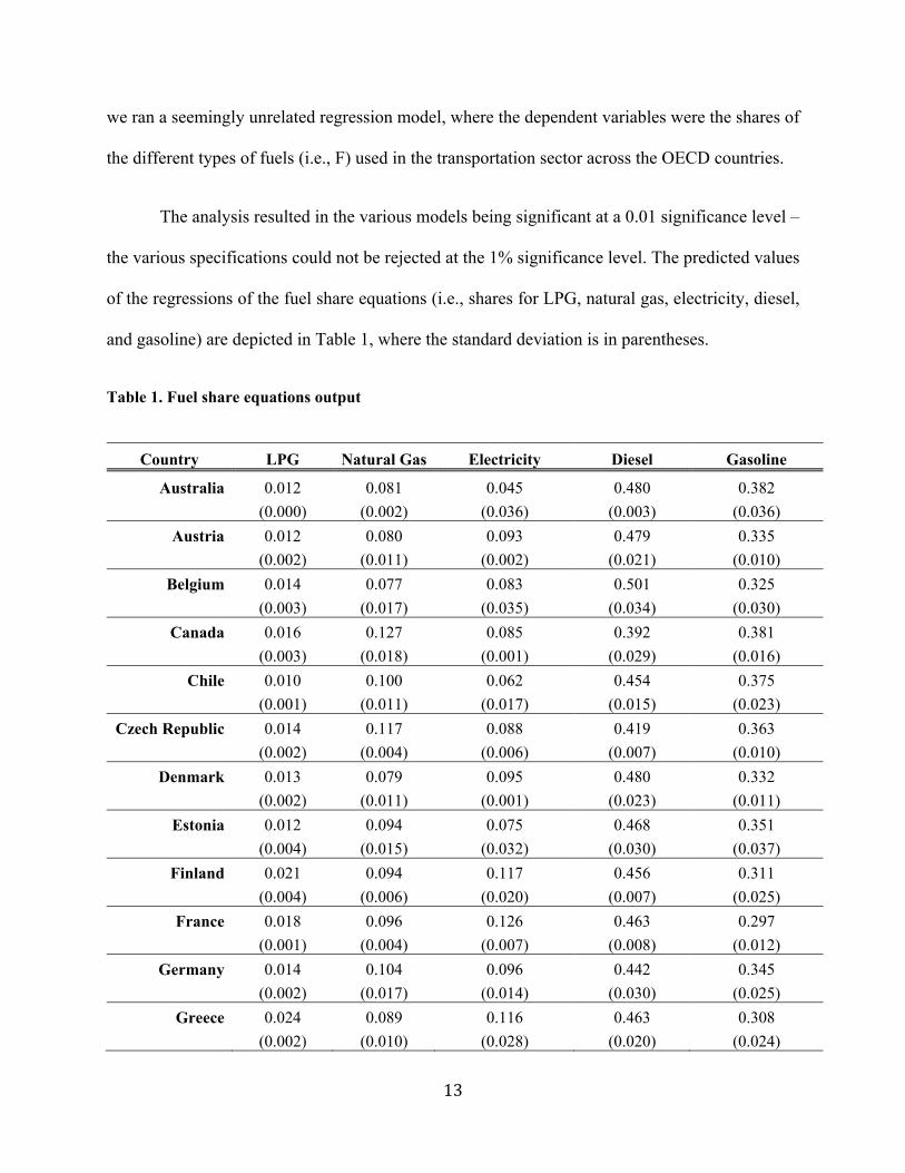
we ran a seemingly unrelated regression model, where the dependent variables were the shares of

the different types of fuels (i.e., F) used in the transportation sector across the OECD countries.

The analysis resulted in the various models being significant at a 0.01 significance level –

the various specifications could not be rejected at the 1% significance level. The predicted values

of the regressions of the fuel share equations (i.e., shares for LPG, natural gas, electricity, diesel,

and gasoline) are depicted in Table 1, where the standard deviation is in parentheses.

Table 1. Fuel share equations output

Country LPG Natural Gas Electricity Diesel Gasoline

Australia 0.012 0.081 0.045 0.480 0.382

(0.000) (0.002) (0.036) (0.003) (0.036)

Austria 0.012 0.080 0.093 0.479 0.335

(0.002) (0.011) (0.002) (0.021) (0.010)

Belgium 0.014 0.077 0.083 0.501 0.325

(0.003) (0.017) (0.035) (0.034) (0.030)

Canada 0.016 0.127 0.085 0.392 0.381

(0.003) (0.018) (0.001) (0.029) (0.016)

Chile 0.010 0.100 0.062 0.454 0.375

(0.001) (0.011) (0.017) (0.015) (0.023)

Czech Republic 0.014 0.117 0.088 0.419 0.363

(0.002) (0.004) (0.006) (0.007) (0.010)

Denmark 0.013 0.079 0.095 0.480 0.332

(0.002) (0.011) (0.001) (0.023) (0.011)

Estonia 0.012 0.094 0.075 0.468 0.351

(0.004) (0.015) (0.032) (0.030) (0.037)

Finland 0.021 0.094 0.117 0.456 0.311

(0.004) (0.006) (0.020) (0.007) (0.025)

France 0.018 0.096 0.126 0.463 0.297

(0.001) (0.004) (0.007) (0.008) (0.012)

Germany 0.014 0.104 0.096 0.442 0.345

(0.002) (0.017) (0.014) (0.030) (0.025)

Greece 0.024 0.089 0.116 0.463 0.308

(0.002) (0.010) (0.028) (0.020) (0.024)

14

Hungary 0.022 0.100 0.113 0.441 0.324

(0.003) (0.010) (0.020) (0.020) (0.033)

Ireland 0.011 0.104 0.063 0.446 0.375

(0.005) (0.004) (0.026) (0.004) (0.030)

Israel 0.015 0.071 0.103 0.505 0.306

(0.004) (0.027) (0.039) (0.046) (0.062)

Italy 0.015 0.079 0.129 0.496 0.281

(0.003) (0.016) (0.003) (0.033) (0.013)

Japan 0.014 0.115 0.078 0.420 0.373

(0.005) (0.007) (0.018) (0.018) (0.010)

Korea, Rep. 0.016 0.108 0.083 0.426 0.367

(0.003) (0.015) (0.003) (0.031) (0.015)

Luxembourg 0.012 0.083 0.117 0.489 0.299

(0.005) (0.014) (0.019) (0.028) (0.028)

Mexico 0.016 0.106 0.090 0.431 0.358

(0.003) (0.018) (0.002) (0.036) (0.016)

Netherlands 0.016 0.088 0.127 0.478 0.291

(0.003) (0.017) (0.006) (0.034) (0.019)

New Zealand 0.017 0.116 0.088 0.410 0.368

(0.001) (0.001) (0.001) (0.003) (0.001)

Norway 0.018 0.049 0.131 0.542 0.260

(0.001) (0.007) (0.007) (0.012) (0.013)

Poland 0.018 0.096 0.125 0.460 0.300

(0.001) (0.003) (0.006) (0.008) (0.011)

Portugal 0.019 0.095 0.117 0.459 0.311

(0.004) (0.010) (0.019) (0.018) (0.024)

Slovak 0.017 0.102 0.115 0.449 0.317

Republic (0.001) (0.003) (0.008) (0.007) (0.013)

Slovenia 0.013 0.093 0.083 0.470 0.341

(0.004) (0.015) (0.036) (0.031) (0.040)

Spain 0.016 0.100 0.111 0.456 0.317

(0.002) (0.003) (0.026) (0.005) (0.029)

Sweden 0.019 0.078 0.083 0.489 0.331

(0.005) (0.019) (0.034) (0.037) (0.026)

Switzerland 0.021 0.097 0.113 0.452 0.318

(0.005) (0.005) (0.027) (0.005) (0.031)

Turkey 0.018 0.097 0.121 0.460 0.304

(0.002) (0.006) (0.008) (0.012) (0.015)

United 0.025 0.087 0.131 0.467 0.291

15

Kingdom (0.001) (0.003) (0.002) (0.004) (0.004)

USA 0.017 0.115 0.087 0.414 0.367

(0.002) (0.004) (0.010) (0.010) (0.006)

The null hypothesis = 0 is rejected at the 1% significance level. The analysis also

suggests that, on average, the share of LPG is about 1% of the fuels used in the transport sector in

OECD countries, for electricity it is 6%, and natural gas about 10%. The shares of diesel and

gasoline, on the other hand, are much larger, at 45% and 37%, respectively.

We next calculate partial own- and cross-price elasticities of substitution. These elasticity

numbers indicate how difficult it would be to reduce fuel consumption and substitution of high

carbon intensive fuels with their low carbon intensive counterparts. We used the translog cost

function to calculate the partial own-price (i.e., ) and cross-price (i.e., ) elasticities (i.e., Eq.

(4)). The estimated average values of these elasticities among the 33 countries are presented in

Table 2.

Table 2. Estimated values of partial own- and cross-price elasticities

LPG Natural gas Electricity Diesel Gasoline

LPG -0.02 0.69 0.15 1.57 -0.43

Natural gas 0.11 -0.07 0.14 -0.68 0.53 Electricity -0.10 0.14 -0.10 0.41 0.25

Diesel 0.03 0.08 0.13 -0.21 0.29

Gasoline 0.01 0.12 0.10 0.37 -0.18

However, changes in fuel prices yield changes in the aggregate energy price index and thus

total energy consumption. This assumption is relaxed when calculating total own- and cross-price

elasticities while using Eq. (5). Total price elasticities account for the change in use of total energy

consumed in the transportation sector, as well as inter-fuel substitution. The total own-price

elasticity of substitution is depicted in Table 3.

16

These estimates are similar to those reported in the literature. For instance, Difiglio and

Fulton (2000) concluded that the own-price elasticity of demand of gasoline is about -0.5, although

Hughes et al. (2008) suggested that demand for gasoline became more inelastic after 2000 for the

light-vehicle fleet. Fouquet (2012) documented a gradual decline in own-price elasticity in the

United Kingdom: While in the 19th century the average long-run own-price elasticity was around

-1.5, it was -0.6 in 2010. However, the elasticity is affected by price volatility, whereby in periods

of high volatility quantity is less responsive to change in price than in periods of less volatility

(Lin & Prince, 2013). Note that this paper goes beyond the existing studies by introducing

additional fuels (i.e., electricity, LPG, and natural gas) used in the transport sector.

Table 3. Estimated values of total own- and cross-price elasticities

LPG Natural gas Electricity Diesel Gasoline

LPG -0.03 0.51 -0.83 4.18 -1.55 Natural gas 0.09 -0.16 0.04 -1.01 0.26

Electricity -0.03 0.05 -0.19 0.04 -0.03 Diesel 0.02 -0.01 0.03 -0.57 0.005

Gasoline -0.006 0.02 0.004 0.003 -0.47

How sensitive are these results to the choice of the own-price elasticity of aggregate energy

(i.e. )? Figure 2 depicts the total own-price elasticity on average, while reducing the elasticity

of aggregate energy by 25% as well as increasing it by 25%. The outcomes suggest that the results

do not vary much for LPG, natural gas and electricity, but that we do observe a more significant

increase in the elasticities of diesel and gasoline (recall that the own-price elasticity of aggregate

energy is multiplied by the share of the fuel in the transportation sector, and that the shares of

diesel and gasoline are significantly larger than those of the other three fuels).

17

Figure 2. Sensitivity analysis on total own-price elasticity in the transportation sector for alternative values of aggregate energy elasticity

How did these elasticities change over time? To answer this question, we split the sample

into two subsamples while dropping the years 2005-2007; that is, we re-estimated the various

parameters and recalculated the elasticities twice: The first estimates limited the data to the years

2000-2004, whereas the second focused on 2008-2012. We then compared total own-price

elasticities for the five transportation fuels across the three estimates; that is, for the samples

including data for 2000-2004, 2008-2012, and for the whole sample (Figure 3). Our results offer

support that the elasticity of gasoline is becoming more inelastic with time. Similar trends are

observed for electricity. However, the analysis suggests a different trend for natural gas and diesel,

where the estimates suggest the elasticity increased with time. To this end, natural gas and diesel

fuels are employed by the power sector and used in heavy duty vehicles. In addition, the

consumption of natural gas and diesel has been expanding substantially during the investigated

period.

-0.7-0.6-0.5-0.4-0.3-0.2-0.10LPG NG Electricity Diesel Gasoline 87

75% of -0.85 (-0.6375) -0.85 125% of -0.85 (-1.0625)

18

Figure 3. Total own-price demand elasticity in the transportation sector for alternative

time periods

5. Concluding remarks

This paper aims to compare the efficacies of two important policies to reduce GHG

emissions from the transport sector: (a) fuel efficiency improvement, and (b) fuel substitution. For

this purpose, we estimated, using a translog cost function, the partial as well as total own-price

elasticity and cross-price elasticity using 15 years’ time-series data from 33 industrialized

economies. While most existing studies (e.g., Greening, 2004; Lu et al. 2007; Timilsina and

Shrestha, 2008; Timilsina and Shrestha 2009) have used a decomposition approach to understand

the role of various factors, such as energy efficiency improvement and fuel switching, on changes

in transport sector CO2 emission intensities, this study uses an econometric approach, which is

-0.7-0.6-0.5-0.4-0.3-0.2-0.10LPG NG Electricity Diesel Gasoline 87

2000-2004 All sample 2008-2012

19

richer in analytical terms, as this technique captures the effects energy prices on its demand and

associated CO2 emissions.

Our study first provides additional estimations of own and cross-price elasticities of fuels

used for transportation, thus further making these elasticity numbers available for transport sector

and economy-wide models for transportation policy analysis. Our results together with findings

from the existing studies suggest that price elasticities of transportation fuels are relatively low

due to limited substitution possibilities among fuels for transportation.

Based on the estimated values of own and cross-price elasticities, this study concludes that

in the industrialized economies a GHG mitigation policy for the transport sector would be more

effective if it aims to improve vehicle efficiency and reduce miles traveled per unit of fuel

consumption. Historical data suggest that the existing fuel pricing policies are not yet capable for

a large-scale switching from existing fleets to electric vehicles. This finding also implies that if the

governments encourage fuel switching, they should either significantly increase prices of

transportation fuels to internalize their environmental damages or adopt regulatory policies that

would mandate switching of fuels, such as employed in India to switch vehicles from gasoline to

LPG. In Norway, the government is implementing an aggressive policy to wean drivers off fossil

fuels and usher in the use of electric vehicles (currently at 2%, the highest in the world). Note that

this type policy to switch over from fossil fuels to electricity may work in Norway due to its

predominant use of hydropower for electricity generation. Similar policy, however, may not

necessarily lead to reduction of CO2 emissions in other countries where fossil fuels are the main

sources for their electricity generation.

20

References

Ang, B.W., Zhang, F.Q., 2000. “A survey of index decomposition analysis in energy and

environmental studies.” Energy. Vol. 25, No. 12: 1149–1176.

Bemdt, ER, and D Wood. 1975. "Technology, Prices, and the Derived Demand for Energy." The

review of Economics and Statistics. Vol. 57. No. 3: 259-268.

Bosetti, V. C Carraro, and M Galeotti. (2006) “The Dynamics of Carbon and Energy Intensity in

a Model of Endogenous Technical Change.” The Energy Journal. Vol. 27: 191-205

Bureau of Labor Statistics: International Labor Comparisons. http://www.bls.gov/fls/

Cullen, JA and ET Mansur. 2014. “Inferring carbon abatement costs in electricity markets: A

revealed preference approach using the shale revolution.” NBER working paper #20795

Difiglio, C and L Fulton. 2000. “How to reduce US automobile greenhouse gas emissions.”

Energy. Vol. 25: 657-673

Gales, B, A Kander, P Malanima, and M Rubio. 2007. “North versus South: Energy transition

and energy intensity in Europe over 200 years.” European Review of Economic History. Vol. 11:

219–253.

Global Wage Report 2012-13: Wages and Equitable Growth.

http://www.ilo.org/global/research/global-reports/global-wage-report/2012/lang--en/index.htm

21

Greening, LA. 2004. "Effects of human behavior on aggregate carbon intensity of personal

transportation: Comparison of 10 OECD Countries for the Period 1970-1993." Economics

Energy. Vol. 26, No. 1: 1-3

Greening, LA, M Ting, and WB Davis. 1999. “Decomposition of aggregate carbon intensity for

freight: trends from 10 OECD countries for the period 1971–1993.” Energy Economics. Vol. 21:

331–361.

Fuss, MA. 1977. "The Demand for Energy in Canadian Manufacturing," Journal of

Econometrics. Vol. 5. No. 1: 89-116.

Fouquet, R. (2012). Trends in income and price elasticities of transport demand (1850–2010).

Energy Policy, 50, 62-71.

Halvorsen, R, and J. Ford. 1978. "Substitution Among Energy, Capital, and Labor Inputs in U.S.

Manufacturing," in R. S. Pindyck (ed.), Advances in the Economics of Energy and resource, Vol.

I. Greenwich, Connecticut: JAI Press.

Hughes, J.E., Knittel, C.R., Sperling, D., 2008. Evidence of a shift in the short-run price

elasticity of gasoline demand. Energy J. 29 (1), 113–134.

International Energy Agency (IEA), 2016a. Energy Balances of Non-OECD countries, 2016

edition. IEA, Paris.

International Energy Agency (IEA), 2016b. CO2 emissions from fossil fuel consumption, 2016

edition. IEA, Paris.

International Energy Agency (IEA), 2014a. CO2 Emissions from Fuel Combustion. IEA, Paris.

22

International Energy Agency (IEA), 2014b. Main Economic Indicators. Volume 2014/11. IEA,

Paris.

International Energy Agency (IEA), 2014c. Energy Statistics OECD. IEA, Paris.

International Energy Agency (IEA), 2014d. Energy Statistic Non-OECD. IEA, Paris.

International Energy Agency (IEA), 2014e. Energy Prices and Taxes: Quarterly Statistics. IEA,

Paris.

IPCC. 1997. Revised 1996 IPCC Guidelines for National Greenhouse Gas Inventories, IPCC/

OECD/IEA, Paris, 1997

IPCC. 2007. Climate Change 2007: Mitigation of Climate Change. Contribution of Working

Group III to the Fourth Assessment Report of the Intergovernmental Panel on Climate Change B.

Metz, O.R. Davidson, P.R. Bosch, R. Dave, L.A. Meyer (eds). Cambridge University Press,

Cambridge, United Kingdom and New York, NY, USA.

Kojima, M. (2009). Changes in end-user petroleum product prices: A comparison of 48

countries. World Bank Extractive Industries and Development Series #2.

Liaoa, H, Y Fana, YM Weia. 2007. “What induced China’s energy intensity to fluctuate: 1997–

2006?” Energy Policy. Vol. 35: 4640-4649

Lin, C. Y. C., & Prince, L. (2013). Gasoline price volatility and the elasticity of demand for

gasoline. Energy Economics, 38, 111-117.

23

Lu, IJ, SJ Lin, and C Lewis. 2007. “Decomposition and decoupling effects of carbon dioxide

emission from highway transportation in Taiwan, Germany, Japan and South Korea.” Energy

Policy. Vol. 35: 3226–3235

McCollum, D, and C Yang . 2009. “Achieving deep reductions in US transport greenhouse gas

emissions: Scenario analysis and policy implications.” Energy Policy. Vol. 37: 5580-5596

Metcalf, GE. 2008. “An Empirical Analysis of Energy Intensity and Its Determinants at the State

Level.” The Energy Journal. Vol. 29, No. 3: 1-26

Morrow, WR, KS Gallagher, G Collantes, and H Lee. 2010. “Analysis of policies to reduce oil

consumption and greenhouse-gas emissions from the US transportation sector.” Energy Policy.

Vol. 38: 1305–1320

Paravantis, JA, and DA Georgakellos. 2007. “Trends in energy consumption and carbon dioxide

emissions of passenger cars and buses.” Technological Forecasting & Social Change. Vol. 74:

682–707

Pindyck, RS. 1979. “Interfuel Substitution and the Industrial Demand for Energy: An

International Comparison.” The Review of Economics and Statistics. Vol. 61, No. 2: 169-179.

Poudenx, P. 2008. “The effect of transportation policies on energy consumption and greenhouse

gas emission from urban passenger transportation.” Transportation Research Part A. Vol. 42:

901-909

Shapiro, JS and R Walker. 2015. “Why is pollution from U.S. manufacturing declining? The

roles of trade, regulation, productivity, and preferences.” NBER working paper #20879.

24

Serletis A., G.R. Timilsina and O. Vasetsky (2010). International Evidence on Sectoral Interfuel

Substitution, The Energy Journal, Vol. 31, No. 4, pp. 1-30.

Timilsina, G.R. and A. Shrestha. 2008. Factors Affecting Transport Sector CO2 Emissions

Growth in Latin American and Caribbean Countries: An LMDI Decomposition Analysis,

International Journal of Energy Research, Vol. 33 No. 4, pp. 396-414,

Timilsina, G.R. and A. Shrestha. 2009. Transport Sector CO2 Emissions Growth in Asia:

Underlying Factors and Policy Options, Energy Policy, Vol. 37, No. 11, pp. 4523-4539.

US EIA [internet]. “Consumption and Efficiency.” 2001. Release date: November 2005 [viewed

2014 January]

US EIA [internet]. “Renewable and Alternative Fuels: Alternative Fuel Vehicle Data.” Released:

April 8, 2013. Next release date: April 2014 [viewed 2014 January]

US Environmental Protection Agency. http://www.epa.gov

Uzawa, H. 1962. “Production functions with constant elasticities of substitution.” The Review of

Economics and Statistics, Vol. 61, No. 2: 291-299.

WDR2013 Occupational Wages around the World. http://data.worldbank.org/data-

catalog/occupational-wages

Weber, CL. 2009. “Measuring structural change and energy use: decomposition of the US

economy from 1997 to 2002.” Energy Policy. Vol. 37: 1561–1570.

World Bank online databank. http://data.worldbank.org/indicator/FR.INR.RINR