From Richardson to early numerical weather predictionplynch/Publications/CMMAP-Pp3-17.pdf · From...

C:/ITOOLS/WMS/CUP/2120402/WORKINGFOLDER/DDO/9780521190060C02.3D 3 [3–17] 27.8.2010 1:06AM

2

From Richardson to early numericalweather prediction

peter lynch

The development of computer models for numerical simulation of the atmosphereand oceans is one of the great scientific triumphs of the past fifty years. Thesemodels have added enormously to our understanding of the complex processes inthe atmosphere and oceans. The consequences for humankind of ongoing climatechange will be far-reaching. Earth system models are the best means we have ofpredicting the future of our climate.The basic ideas of numerical forecasting and climate modeling were developed

about a century ago, long before the first electronic computer was constructed.However, advances on several fronts were necessary before numerical predictioncould be put into practice. A fuller understanding of atmospheric dynamics allowedthe development of simplified systems of equations; regular observations of thefree atmosphere provided the initial conditions; stable finite difference schemeswere developed; and powerful electronic computers provided a practical means ofcarrying out the calculations required to predict the changes in the weather.In this chapter, we trace the history of computer forecasting from Richardson’s

prodigious manual computation, through the ENIAC (Electronic NumericalIntegrator and Computer) integrations to the early days of operational numericalweather prediction and climate modeling. The useful range of deterministic pre-diction is increasing by about one day each decade. We set the scene for the storyof the remarkable progress in weather forecasting and in climate modeling overthe past fifty years, which will be treated in subsequent chapters.

2.1 Pioneers of scientific forecasting

The fundamental idea of computing changes in the weather by numerical means wasformulated around the turn of the twentieth century, before electronic computerswere available. The great American meteorologist Cleveland Abbe recognized thatmeteorology is essentially the application of hydrodynamics and thermodynamics

3


to the atmosphere (Abbe, 1901), and he identified the system of mathematicalequations that govern the evolution of the atmosphere. Abbe’s work was reviewedrecently by Willis and Hooke (2006). The Norwegian scientist Vilhelm Bjerknesundertook a more explicit analysis of the weather prediction problem from ascientific perspective (Bjerknes, 1904). His stated goal was to make meteorologyan exact science, a true physics of the atmosphere.Later, Lewis Fry Richardson (Figure 2.1) attempted a direct solution of the

equations of motion, and presented the results in his book Weather Prediction byNumerical Process (Richardson, 1922). The book opened with a discussion ofthen-current practice. Richardson described the use of an index of weathermaps, constructed by classifying old synoptic charts into categories. The indexassisted the forecaster to find previous maps resembling the current one and thusdeduce the likely development by studying the evolution of these earlier cases.This “analog approach” was at the heart of operational forecasting until themodern era, and forecast skill remained rather static. Indeed, Sverre Petterssen(2001) described the advances prior to the computer era as occurring in “homeo-pathic doses”.

Figure 2.1 Lewis Fry Richardson (1881–1953), signed and dated 1931, whenRichardson was aged 50 (photograph by Walter Stoneman; copy courtesy ofOliver Ashford).

4 The Development of Atmospheric General Circulation Models


The full story of Richardson’s work, the reason for his catastrophic results, and acomplete reconstruction of the forecast are described in a recent book (Lynch,2006). Richardson calculated a change in surface pressure over a six-hour periodof 145 hPa, a totally unrealistic value. His extrapolation over six hours exacerbatedthe problem, but was not the root cause of it. Lynch showed that, when the analyzeddata are balanced through the process of initialization, a realistic value of pressurechange is obtained. In Table 2.1 we show the six-hour changes in pressure at eachlevel of the numerical model he used. The column marked LFR (Lewis FryRichardson) has the values obtained by Richardson (1922). The column markedMOD (model) has the values reconstructed using a computer model based directlyon Richardson’s method: they are very close to Richardson’s values. The columnmarked DFI (digital filter initialization) is for a forecast from data initialized using adigital filter: the initial tendency of surface pressure is reduced from the unrealistic145 hPa/6 h to a reasonable value of less than 1 hPa/6 h (bottom row, Table 2.1).These results indicate clearly that Richardson’s unrealistic prediction was due toimbalance in the initial data that he used. Complete details of the forecast recon-struction may be found in Lynch (2006).Richardson’s forecasting scheme involved a phenomenal volume of numerical

computation and was quite impractical in the pre-computer era. But he wasundaunted, speculating that

“some day in the dim future it will be possible to advance the computations faster than theweather advances”.

The work of Max Margules, published almost twenty years before Richardson’sforecast, pointed to serious problems with Richardson’s methodology. Margulesexamined the relationship between the continuity equation (which expresses con-servation of mass) and changes in surface pressure (Margules, 1904). He consideredthe possibility of predicting pressure changes by direct use of the mass conservationprinciple. He showed that, due to strong cancellation between terms, the calculation

Table 2.1 Six-hour changes in pressure (units: hPa/6 h).[LFR: Richardson; MOD: Model; DFI: Filtered.]

Level (km) LFR MOD DFI

1 (11.8) 48.3 48.5 −0.22 (7.2) 77.0 76.7 −2.63 (4.2) 103.2 102.1 −3.04 (2.0) 126.5 124.5 −3.1Surface 145.1 145.4 −0.9

From Richardson to early numerical weather prediction 5


is very error-prone, and may give ridiculous results. Therefore, it is not possible,using the continuity equation alone, to derive a reliable estimate of synoptic-scalechanges in pressure. Margules concluded that any attempt to forecast the weatherwas immoral and damaging to the character of a meteorologist (Fortak, 2001).To make his forecast of the change in pressure, Richardson used the continuity

equation, employing precisely the method that Margules had shown to be seriouslyproblematical. The resulting prediction of pressure change was completely unrea-listic. The question of what influence, if any, Margules’ results had on Richardson’sapproach to forecasting was considered by Lynch (2003). At a later stage,Richardson did come to a realization that his original method was unfeasible. In anote contained in the Revision File, inserted in the manuscript version of his book,he wrote,

“Perhaps the most important change to be made in the second edition is that the equation ofcontinuity of mass must be eliminated”.

(Richardson’s underlining)

He went on to speculate that the vertical component of vorticity or rotation rate ofthe fluid might be a suitable prognostic variable. This was indeed a visionaryadumbration of the use of the vorticity equation for the first successful numericalintegration in 1950.Of course, we now know that Margules was unduly pessimistic. The continuity

equation is an essential component of primitive equation models which are used inthe majority of current computer weather prediction systems. Primitive equationmodels use the exact equations of motion except for the hydrostatic approximation:they support gravity wave solutions and, when changes in pressure are computedusing the continuity equation, large tendencies can arise if the atmospheric condi-tions are far from balance. However, spuriously large tendencies are avoided inpractice by an adjustment of the initial data to reduce gravity wave components torealistic amplitudes, by the process of initialization, as indicated in Table 2.1.

2.2 Pre-computer forecasting

Weather forecasts are now so reliable, accurate, and readily available that it is easyto forget how things were only a few decades ago. Before the computer era,forecasting was imprecise and undependable. Analysis of the global atmosphericstate was severely hampered by lack of observations, and the principles of theore-tical physics played little role in practical forecasting. Although much of the under-lying physics was known, its application to the prediction of atmospheric conditionswas impractical. Observations were sparse and irregular, especially for the upper airand over the oceans.



Forecasting was a haphazard process, very imprecise and unreliable. The fore-caster used crude techniques of extrapolation, knowledge of local climatology, andguesswork based on intuition; forecasting was more an art than a science. Theobservations of pressure and other variables were plotted in symbolic form ona weather map and lines were drawn through points with equal pressure to revealthe pattern of weather systems – depressions, anticyclones, troughs, and ridges. Theforecaster used experience, memory, and a variety of empirical rules to produce aforecast map. The primary physical process attended to by the forecaster wasadvection, the transport of fluid characteristics and properties by the movement ofthe fluid itself. But the crucial quality of advection is that it is nonlinear; the humanforecaster may extrapolate trends using an assumption of constant wind, but is quiteincapable of intuiting the subtleties of complex advective processes.The technique of “weather typing” was used with limited success. This was the

method underlying the index of weather maps, mentioned by Richardson. Currentmeteorological conditions were compared with the historical record. If a closematch was found, it was assumed that the evolution of the flow for the followingdays would be similar to that observed on the previous occasion. However, theatmosphere shows little tendency to repeat itself. Richardson was not optimisticabout this method. He wrote in his Preface that

“The forecast is based on the supposition that what the atmosphere did then, it will do againnow . . . The past history of the atmosphere is used, so to speak, as a full-scale workingmodel of its present self”.

(Richardson, 1922)

Bjerknes had contrasted the precision of astronomical prediction with the “radicallyinexact” methods of weather forecasting. Richardson returned to this theme, poin-ting out that the Nautical Almanac,

“that marvel of accurate forecasting”

is not based on the principle that astronomical history repeats itself. Given thecomplexity of the atmosphere, why should we expect a present weather map to beexactly represented in a catalogue of past weather?In Europe meteorology was studied in many universities, and researchers applied

physical principles to atmospheric problems. Bjerknes had dreamed of mathema-tical forecasting but, finding it impractical, had marshaled his team in Bergen todevelop more feasible methods. They developed mechanistic models of extra-tropical weather systems and described the life-cycles of mid-latitude depressionsand their associated warm and cold fronts. Although the models of polar fronts andthe life-cycles of extra-tropical depressions are conceptual in nature, they arefounded on sound scientific principles. Frontal and air-mass theory gradually



came to have a profound influence on operational practice on both sides of theAtlantic. Bjerknes visited America to promote the new ideas and many of hisBergen students played major roles in the advancement of American meteorology,both in government agencies and universities.

2.3 Key developments, 1920–1950

Richardson was several decades ahead of his time in what he attempted to do. At thetime of the First World War, computational weather forecasting was impractical forat least four reasons.First, observations of the three-dimensional structure of the atmosphere were

available only on a very occasional basis, with inadequate coverage and never inreal time. The registering balloons had to be recovered and the recordings analyzedto recover the data, a process that took days or even weeks. Second, the numericalalgorithms for solving the atmospheric equations were subject to instabilities thatwere not understood. Thus, the numerical solution might bear little or no resem-blance to the solution of the continuous equations. Third, the balanced nature ofatmospheric flow was inadequately understood, and the imbalances arising fromobservational and analysis errors confounded Richardson’s forecast. Fourth, themassive volume of computation required to advance the numerical solution couldnot be done, even by a huge team of human computers. Indeed, Richardson’sestimate of 64,000 computers, the number of people needed to do the calculationsfor a useful forecast in real time, was a serious under-estimate. It has been reckonedthat one million people would have been required for the task (Lynch, 1993). Thus,what Richardson devised was a “method without a means”.A number of key developments in the ensuing decades set the scene for progress.

Developments in the theory of meteorology provided crucial understanding of atmo-spheric dynamics, in particular the balance of the atmosphere and the means ofeliminating spurious high-frequency gravity waves. Advances in numerical analysisled to the design of algorithms which were stable and faithfully replicated the truesolution. Timely observations of the atmosphere in three dimensions were becomingavailable following the invention of the radiosonde, which providedmeasurements ofpressure, temperature, humidity, and winds through a vertical column of the atmo-sphere. Finally, the development of digital computers provided a way of attacking theenormous computational task involved in weather forecasting.In addition to the technical developments, the socio-political framework of the

mid century provided a crucial impetus. Progress in meteorology has often followedfrom natural or human-made catastrophes. The SecondWorldWar was a spectacularexample. Military operations on land, air, and sea all depend heavily on accurateweather forecasts. The role of weather in Operation Overlord – the D-day invasion



of Normandy –was recounted by Pettersen (2001). In the United States an intensivetraining program for meteorologists was organized under the inspiration of Carl-Gustav Rossby. As a result, the professional meteorological community grew by afactor of fifteen during the war, from 400 before to 6000 afterwards. Many of thenew entrants were highly skilled in mathematics and physics and wished to developrigorous methods of forecasting that were based on scientific principles.

2.4 The ENIAC integrations

The first general-purpose electronic computer, ENIAC (Electronic NumericalIntegrator and Computer) was commissioned by the U.S. Army for use in calculat-ing the dynamics of projectiles. The principal designers of ENIAC were JohnMauchly and Presper Eckert. It is noteworthy that Mauchley’s interest in computersarose from his desire to forecast the weather by calculation. The computer wasoriginally called the Electronic Numerical Integrator. A U.S. Army colonel sug-gested adding the words “and Computer” to give the catchy acronym ENIAC(McCartney, 1999). The ENIAC, which had been completed in 1945, was the firstgeneral-purpose electronic digital computer ever built. It was a gigantic machine,with 18,000 thermionic valves, filling a large room and consuming 140 kW ofpower. Input and output were by means of punch-cards. McCartney (1999) providesan absorbing account of the origins, design, development, and destiny of ENIAC.John von Neumann recognized weather forecasting, a problem of both great

practical significance and intrinsic scientific interest, as ideal for an automatic compu-ter. Hewas in close contact with Rossby, whowas the person best placed to understandthe challenges that would have to be addressed to achieve success in this venture. VonNeumann established a Meteorology Project at the Institute for Advanced Study inPrinceton and recruited Jule Charney to lead it. Arrangements were made to compute asolution of a simple equation, the barotropic vorticity equation (BVE), on the onlycomputer available, the ENIAC. Barotropic models treat the atmosphere as a singlelayer, averaging out variations in the vertical. The resulting numerical predictions weretruly ground-breaking. Four 24-hour forecasts were made, and the results clearlyindicated that the large-scale features of the mid-tropospheric flow could be forecastnumerically with a reasonable resemblance to reality.The ENIAC forecasts were described in a seminal paper by Jule Charney, Ragnar

Fjørtoft, and John von Neumann (Charney, et al., 1950, referenced below as CFvN).The story of this work was recounted by George Platzman in his Victor P. StarrMemorial Lecture (Platzman, 1979). The atmosphere was treated as a single layer,represented by conditions at the 500 hPa level, modeled by the BVE. This equation,expressing the conservation of absolute vorticity following the flow, gives the rate ofchange of the Laplacian of the height of the 500 hPa surface in terms of the



advection. The tendency of the height field is obtained by solving a Poissonequation with homogeneous boundary conditions. The height field may then beadvanced to the next time level. With a one-hour timestep, this cycle is repeated24 times for a one-day forecast.The initial data for the forecasts were prepared manually from standard opera-

tional 500 hPa analysis charts of the U.S. Weather Bureau, discretized to a grid of19 by 16 points, with grid interval of 736 km. Centered spatial finite differences anda leapfrog time-scheme were used. The boundary values of height were heldconstant throughout each 24-hour integration. The forecast starting at 0300 UTC,January 5, 1949 is shown in Figure 2.2 (fromCFvN). The left panel is the analysis of500 hPa height and absolute vorticity. The forecast height and vorticity are shown inthe right panel. The feature of primary interest was an intense depression over theUnited States. This deepened, moving NE to the 90°W meridian in 24 hours.A discussion of this forecast, which underestimated the development of the depres-sion, may be found in CFvN and in Lynch (2008).The success of the ENIAC forecasts had an electrifying effect on the world

meteorological community. Several baroclinic (multi-level) models were developedin the following years. They were all based on the filtered or quasi-geostrophicsystem of equations, an approximate system derived using geostrophic balancebetween the pressure and winds. Later, models using the more accurate primitiveequations were introduced. Charney had anticipated this as a necessary develop-ment, and indeed André Robert later identified it as the key development innumerical weather prediction (see Lin et al. 1997).

Figure 2.2 The ENIAC forecast starting at 0300 UTC, January 5, 1949. Leftpanel: analysis of 500 hPa height (thick lines) and absolute vorticity (thin lines).Right panel: forecast height and vorticity (from Charney, et al., 1950). Height unitsare hundreds of feet, contour interval is 200 ft. Vorticity units and contour intervalare 10−5s−1.



The Princeton team studied the severe storm of Thanksgiving Day, 1950using two-and three-level quasi-geostrophic models. After some tuning, theyfound that the cyclogenesis could be reasonably well simulated. Thus, itappeared that the central problem of operational forecasting had been cracked.However, it transpired that the success of the Thanksgiving forecast had beensomething of a fluke: early multi-level models were consistently worse than thesimple barotropic equation; and it was the single-level model that was usedwhen regular operations commenced in 1958. A fuller discussion can be foundin Lynch (2006). The trials and triumphs of the Joint Numerical WeatherPrediction Unit, which will appear again in Chapter 3, and the establishmentof operational computer forecasting are described comprehensively in a recentbook (Harper, 2008).

2.5 Advancing computer technology

Advances in computer technology over the past half-century have been spec-tacular. The increase in computing power is encapsulated in an empirical rulecalled Moore’s Law, which implies that computing speed doubles about every18 months. Thus, a modern micro-processor has far greater power than the ENIAChad. Recently, Lynch & Lynch (2008) decided to repeat the ENIAC integrationsusing a programmable cell-phone, which was called the Portable Hand-OperatedNumerical Integrator and Computer, or PHONIAC. This technology has greatpotential for generation and display of operational weather forecast products.The oft-cited paper in Tellus (CFvN) gives a complete account of the computa-

tional algorithm and discusses four forecast cases. Lynch (2008) presented theresults of repeating the ENIAC forecasts using a Matlab program eniac.m,run on a laptop computer (a Sony Vaio, model VGN-TX2XP). The main loop of the24-hour forecast ran in about 30 ms. Given that the original ENIAC integrationseach took about one day, this time ratio – about three million to one – indicates thedramatic increase in computing power over the past half-century. The programeniac.m was converted from Matlab to a Java application, phoniac.jar,for implementation on a cell-phone. The program was tested on a PC usingemulators for three different mobile phones. A basic graphics routine was alsowritten in Java.Whenworking correctly, the programwas downloaded onto a Nokia6300 cell-phone for execution.Charney et al. (1950) provided a full description of the solution algorithm for the

BVE. The programs eniac.m and phoniac.jar were constructed followingthe original algorithm precisely, including the specification of the boundary condi-tions and the Fourier transform solution method for the Poisson equation. Hence,given initial data identical to that used in CFvN, the recreated forecasts should be



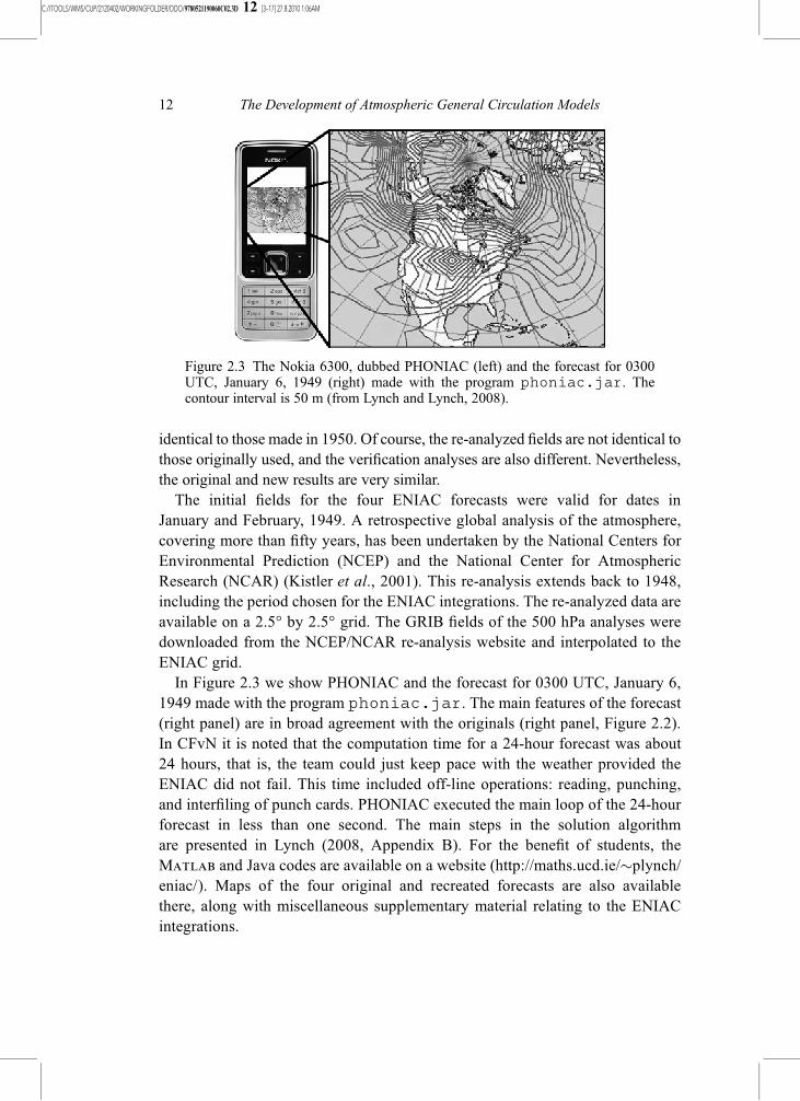
identical to those made in 1950. Of course, the re-analyzed fields are not identical tothose originally used, and the verification analyses are also different. Nevertheless,the original and new results are very similar.The initial fields for the four ENIAC forecasts were valid for dates in

January and February, 1949. A retrospective global analysis of the atmosphere,covering more than fifty years, has been undertaken by the National Centers forEnvironmental Prediction (NCEP) and the National Center for AtmosphericResearch (NCAR) (Kistler et al., 2001). This re-analysis extends back to 1948,including the period chosen for the ENIAC integrations. The re-analyzed data areavailable on a 2.5° by 2.5° grid. The GRIB fields of the 500 hPa analyses weredownloaded from the NCEP/NCAR re-analysis website and interpolated to theENIAC grid.In Figure 2.3 we show PHONIAC and the forecast for 0300 UTC, January 6,

1949 made with the program phoniac.jar. The main features of the forecast(right panel) are in broad agreement with the originals (right panel, Figure 2.2).In CFvN it is noted that the computation time for a 24-hour forecast was about24 hours, that is, the team could just keep pace with the weather provided theENIAC did not fail. This time included off-line operations: reading, punching,and interfiling of punch cards. PHONIAC executed the main loop of the 24-hourforecast in less than one second. The main steps in the solution algorithmare presented in Lynch (2008, Appendix B). For the benefit of students, theMatlab and Java codes are available on a website (http://maths.ucd.ie/�plynch/eniac/). Maps of the four original and recreated forecasts are also availablethere, along with miscellaneous supplementary material relating to the ENIACintegrations.

Figure 2.3 The Nokia 6300, dubbed PHONIAC (left) and the forecast for 0300UTC, January 6, 1949 (right) made with the program phoniac.jar. Thecontour interval is 50 m (from Lynch and Lynch, 2008).



2.6 Climate modeling

We can trace the beginnings of climate modeling back to 1956, when NormanPhillips carried out the first long-range simulation of the general circulation of theatmosphere. He used a two-level quasi-geostrophic model on a beta-plane channel,ignoring the effects of sphericity except for variations of the Coriolis force withlatitude. The computation used a spatial grid of 16 × 17 points, and the simulationwas for a period of about one month. Starting from a zonal flow with small randomperturbations, a wave disturbance with a wavelength of 6000 km developed. It hadthe characteristic westward tilt with the height of a developing baroclinic wave, andmoved eastward at about 20m s−1. Figure 2.4 shows the configuration of the flowafter twenty days’ simulation. Phillips examined the energy exchanges of thedeveloping wave and found good qualitative agreement with observations ofbaroclinic systems in the atmosphere. He also examined the mean meridionalflow, the average circulation in a vertical cross-section along a meridian, andfound circulations corresponding to the Hadley, Ferrel, and Polar cells, large-scale

Figure 2.4 Configuration of the flow after 20-days’ simulation with a simple,two-level filtered model. Solid lines: 1000 hPa heights at 200 foot intervals.Dashed lines: 500 hPa temperatures at 5 °C intervals (Phillips, 1956).



circulations with ascending motion at one latitude coupled to descending motion atanother through meridional flow:

“We see the appearance of a definite three-celled circulation, with an indirect [or reverse]cell in middle latitudes and two somewhat weaker cells to the north and south. This is acharacteristic feature of . . . unstable baroclinic waves”.

(Phillips, 1956, p. 144)

Von Neumann was hugely impressed by Phillips’ work, and arranged a conferenceat Princeton University in October 1955, Application of Numerical IntegrationTechniques to the Problem of the General Circulation, to consider its implications.The work had a galvanizing effect on the meteorological community. Within tenyears, there were several major research groups modeling the general circulation ofthe atmosphere, the leading ones being at the Geophysical Fluid DynamicsLaboratory, the National Center for Atmospheric Research, the University ofCalifornia, Los Angeles, the Lawrence Livermore National Laboratory, and theUnited Kingdom Meteorological Office These research efforts will appear again inChapters 3 and 9.The development of comprehensive models of the atmosphere is undoubtedly

one of the finest achievements of meteorology in the twentieth century. FollowingPhillips’ seminal work, several general circulation models (GCMs) were developed,including various physical processes such as solar heating, terrestrial radiation,convection, and small-scale turbulence. Advanced models are under continuingrefinement and extension, and are increasing in sophistication and comprehensive-ness. They simulate not only the atmosphere and oceans but also a wide range ofgeophysical, chemical, and biological processes and feedbacks. The models, nowcalled Earth system models, are applied to the eminently practical problem ofweather prediction and also to the study of climate variability and humankind’simpact on it. There is no doubt that the study of climate change and its impacts is ofenormous importance for our future. Global climate models are the best means wehave of anticipating likely changes.

2.7 Uncertainty and probability

The chaotic nature of the atmospheric flow, most clearly elucidated by Lorenz(1963), imposes a limit on predictability, as unavoidable errors in the initial stategrow rapidly and render the forecast useless after some days. The most successfulmeans of confronting this obstacle is to run a collection, or ensemble, of forecasts,each starting from a slightly different initial state, and to use the combined outputs todeduce probabilistic information about future changes in the atmosphere.Probability forecasts for a wide range of weather events are generated for use in



the operational centers. These have become the key guidance for medium-rangeprediction.Computer prediction models are now the primary input for operational fore-

casters and are vital for a wide range of applications. Perhaps the most importantapplication is to provide timely warning of weather extremes. The ensembleapproach provides valuable quantitative guidance on the probability and likelyseverity of extreme events. The warnings which result from computer guidanceenable great saving of life and property.Transportation, energy consumption, construction, tourism, and agriculture are

all sensitive to weather conditions. There are expectations from all these sectors ofincreasing accuracy and detail of forecasts, as decisions with heavy financialimplications must continually be made. Numerical weather prediction modelsare used to generate special guidance for the marine community. Trajectories formodeling pollution drift, for nuclear fallout, and smoke from forest fires are easilyderived. Aviation benefits significantly from computer guidance, which provideswarnings of hazards. Automatic generation of terminal aerodrome forecasts enablesservicing of a large number of airports from a central forecasting facility.Interaction between the atmosphere and ocean becomes a dominant factor

at longer forecast ranges. For seasonal forecasting, coupled atmosphere–oceanmodels are essential. Once again, the ensemble approach is an effective means ofaddressing uncertainty in the predictions. Good progress has been made in seaso-nal forecasting for the tropics. Considerable effort is being made to produce usefullong-range forecasts for temperate regions, but many challenges remain. Theensemble approach has also become a central aspect of climate change prediction.

2.8 Dreams fulfilled

Developments in atmospheric dynamics, instrumentation, observing practice, anddigital computing have made the dreams of Abbe, Bjerknes, and Richardson aneveryday reality. Numerical weather prediction models are now at the center ofoperational forecasting. It is no exaggeration to describe the advances made over thepast half-century as revolutionary. Progress in weather forecasting and in climatemodeling has been dramatic. We can now predict the weather for several days inadvance with a high degree of confidence, and the useful range of deterministicprediction is increasing by about one day each decade. Using Earth system models,we are gaining great insight into the factors causing changes in our climate, and theirlikely timing and severity.Meteorology is now firmly established as a quantitative science, and its value and

validity are demonstrated daily by the acid test of any science, its ability to predictthe future. The development of comprehensive models of the atmosphere is



undoubtedly one of the finest achievements of meteorology in the twentieth century.The story of how the models have developed over the past fifty years, and thecurrent state of numerical weather prediction and climate modeling, is told in thefollowing chapters of this volume.

References

Abbe, C. (1901). The physical basis of long-range weather forecasts. Monthly WeatherReview, 29, 551–61.

Bjerknes, V. (1904). Das Problem der Wettervorhersage, betrachtet vom Standpunkte derMechanik und der Physik. Meteorologische Zeitschrift, 21, 1–7.

Charney, J. G., Fjörtoft, R., and von Neumann, J. (1950). Numerical integration of thebarotropic vorticity equation. Tellus, 2, 237–254.

Fortak, H. (2001). Felix Maria Exner und die österreichische Schule der Meteorologie.Pp. 354–386, in Hammerl, Christa,Wolfgang Lenhardt, Reinhold Steinacker, and PeterSteinhauser, 2001: Die Zentralanstalt für Meteorologie und Geodynamik 1851–2001.150 Jahre Meteorologie und Geophysik in Österreich. Leykam Buchverlags GmbH,Graz. ISBN 3–7011–7437–7.

Harper, K. J. (2008). Weather by the Numbers: the Genesis of Modern Meteorology. MITPress, 308pp.

Kistler, R., Kalnay, E., Collins, W., Saha, S., White, G., Woollen, J., Chelliah, M.,Ebisuzaki, W., Kanamitsu, M., Kousky, V., van den Dool, H., Jenne, R., andFiorino, M. (2001). The NCEP-NCAR 50-year reanalysis: Monthly meansCD-ROM and documentation. Bulletin of the American Meteorological Society,82, 247–267.

Lin, C. A., Laprise, R., and Richie, H. ed. (1997). Numerical Methods in Atmospheric andOceanic Modelling. The André J. Robert Memorial Volume. Canadian Meteorologicaland Oceanographic Society.

Lorenz, E. N. (1963) Deterministic nonperiodic flow. Journal of the Atmospheric Sciences,20, 130–141.

Lynch, P. (1993). Richardson’s forecast factory: the $64,000 question. MeteorologicalMagazine, 122, 69–70.

Lynch, P. (2003). Margules’ tendency equation and Richardson’s forecast. Weather, 58,186–193.

Lynch, P. (2006). The Emergence of Numerical Weather Prediction: Richardson’s Dream.Cambridge University Press, 279 pp. (ISBN: 0–521–85729–5).

Lynch, P. (2008). The ENIAC forecasts: a recreation. Bulletin of the AmericanMeteorological Society, 89, 45–55.

Lynch, P. and Lynch, O. (2008). Forecasts by PHONIAC. Weather, 63, 324–326.McCartney, S. (1999). ENIAC: The Triumphs and Tragedies of the World’s First Computer.

Berkley Books, New York, 262pp.Margules, M., (1904). Über die Beziehung zwischen Barometerschwankungen

und Kontinuitätsgleichung [On the relationship between barometric variationsand the continuity equation]. Ludwig Boltzmann Festschrift. Leipzig, Barth, J. A.,930 pp.

Petterssen, S. (2001).Weathering the Storm. Sverre Petterssen, the D-Day Forecast, and theRise of Modern Meteorology. Fleming, J. R. ed. American Meteorological Society.

Phillips, N. A. (1956). The general circulation of the atmosphere : A numerical experiment.Quarterly Journal of the Royal Meteorological Society, 82, 123–164.



Platzman, G.W. (1979). The ENIAC computations of 1950 –Gateway to numerical weatherprediction. Bulletin of the American Meteorological Society, 60, 302–312.

Richardson, L. F. (1922).Weather Prediction by Numerical Process. Cambridge UniversityPress. 2nd Edn. with Foreward by Peter Lynch (2007).

Willis, E. P. and Hooke, W.H. (2006). Cleveland Abbe and American meteorology,1871–1901. Bulletin of the American Meteorological Society, 87, 315–26.


From Richardson to early numerical weather predictionplynch/Publications/CMMAP-Pp3-17.pdf · From...

Documents

Transcript of From Richardson to early numerical weather predictionplynch/Publications/CMMAP-Pp3-17.pdf · From...