From Micro to Macro: Demand, Supply, and Heterogeneity … · From Micro to Macro: Demand, Supply,...

From Micro to Macro: Demand, Supply, and Heterogeneity in the

Trade Elasticity∗

Maria Bas† Thierry Mayer‡ Mathias Thoenig §

September 16, 2015

Abstract

Models of heterogeneous firms with selection into export market participation generically exhibit ag-gregate trade elasticities that vary across country-pairs. Only when heterogeneity is assumed Pareto-distributed do all elasticities collapse into an unique elasticity, estimable with a gravity equation. Thispaper provides a theory-based method for quantifying country-pair specific elasticities when movingaway from Pareto, i.e. when gravity does not hold. Combining two firm-level customs datasets forwhich we observe French and Chinese individual sales on the same destination market over the 2000-2006 period, we are able to estimate all the components of the dyadic elasticity: i) the demand-sideparameter that governs the intensive margin and ii) the supply side parameters that drive the extensivemargin. These components are then assembled under theoretical guidance to calculate bilateral aggre-gate elasticities over the whole set of destinations, and their decomposition into different margins. Ourpredictions fit well with econometric estimates, supporting our view that micro-data is a key elementin the quantification of non-constant macro trade elasticities.

Keywords: trade elasticity, firm-level data, heterogeneity, gravity, Pareto, log-normal.

JEL Classification: F1

∗This research has received funding from the European Research Council under the European Community’s SeventhFramework Programme (FP7/2007-2013) Grant Agreement No. 313522. We thank David Atkin, Dave Donaldson, SwatiDhingra, Ben Faber, Pablo Fagelbaum, Jean Imbs, Oleg Itskhoki, Jan de Loecker, Peter Morrow, Steve Redding, AndresRodriguez Clare, Esteban Rossi-Hansberg, Katheryn Russ, Nico Voigtlander, and Yoto Yotov for useful comments on anearly version, and participants at seminars in UC Berkeley, UCLA, Banque de France, WTO, CEPII, ISGEP in Stockholm,University of Nottingham, Banca d’Italia, Princeton University and CEMFI.†University of Paris 1.‡Sciences Po, Banque de France, CEPII and CEPR. Email: [email protected]. Postal address: 28, rue des

Saints-Peres, 75007 Paris, France.§Faculty of Business and Economics, University of Lausanne and CEPR.

1

1 Introduction

The response of trade flows to a change in trade costs, the aggregate trade elasticity, is a central element inany evaluation of the welfare impacts of trade liberalization. Arkolakis et al. (2012) recently showed thatthis parameter, denoted ε for the rest of the paper, is actually one of the (only) two sufficient statisticsneeded to calculate Gains From Trade (GFT) under a surprisingly large set of alternative modelingassumptions—the ones most commonly used by recent research in the field. Measuring those elasticitieshas therefore been the topic of a long-standing literature in international economics. The most commonusage (and the one recommended by Arkolakis et al., 2012) is to estimate this elasticity in a macro-levelbilateral trade equation referred to as structural gravity in the literature following the initial impulseby Anderson and van Wincoop (2003). In order for this estimate of ε to be relevant for a particularexperiment of trade liberalization, it is crucial for this bilateral trade equation to be correctly specifiedas a structural gravity model with, in particular, a unique elasticity to be estimated across dyads.

Our starting point is that the model of heterogeneous firms with selection into export market par-ticipation (Melitz, 2003) will in general exhibit a dyad-specific elasticity, i.e. an εni, which applies toeach country pair. Only when heterogeneity is assumed Pareto-distributed do all εni collapse to a singleε. Under any other distributional assumption, obtaining an estimate of the aggregate trade elasticityfrom a macro-level bilateral trade equation becomes problematic, since there is a now a whole set of εnito be estimated, and structural gravity does not hold anymore. We argue that in this case quantifyingtrade elasticities at the aggregate level makes it necessary to use micro-level information. To this purposewe exploit a rich panel that combines sales of French and Chinese exporters over 2000-2006 on manydestination-product combinations for which we also observe the applied tariff. We propose a theory-based method using this firm-level export data for estimating all the components of the dyad-specifictrade elasticity: i) the demand-side parameter that governs the intensive margin and ii) the supply sideparameters that drive the extensive margin. These components are then assembled under theoreticalguidance to calculate the dyadic aggregate elasticities over the whole set of destination-product.

Taking into account cross-dyadic heterogeneity in trade elasticities is crucial for quantifying the ex-pected impact of various trade policy experiments.1 Consider the example of the current negotiationsover a transatlantic trade agreement between the USA and the EU (TTIP). Under the simplifying as-sumption of a unique elasticity, whether the trade liberalization takes place with a proximate vs distant,large vs small economy, etc. is irrelevant in terms of trade-promoting effect or welfare gains calculations.By contrast, our results suggest that the relevant εni should be smaller (in absolute value) than if theUnited States were considering a comparable agreement with countries where the expected volume oftrade is smaller. Regarding welfare, Melitz and Redding (2015) and Head et al. (2014) have shown theo-retically that the GFT can be quite substantially mis-estimated if one assumes a constant trade elasticitywhen the “true” elasticity is variable (the margin of error can exceed 100 percent in both papers). Theexpected changes in trade patterns and welfare effects of agreements such as TTIP will therefore bedifferent compared to the unique elasticity case. One of the main objectives of our paper is to quantifyhow wrong can one be when making predictions based on a constant trade elasticity assumption.

Our approach maintains the traditional CES (σ) demand system combined with monopolistic com-petition. It features several steps that are structured around the following decomposition of aggregatetrade elasticity into the sum of the intensive margin and the (weighted) extensive margin:

εni = 1− σ︸︷︷︸intensive margin

+1

xni/xMINni︸︷︷︸min-to-mean

× d lnNni

d ln τni︸︷︷︸extensive margin

, (1)

1Imbs and Mejean (2015) and Ossa (2015) recently argued that another source of heterogeneity, the cross-sectoral one,raises important aggregation issues that matter for aggregate outcomes of trade liberalization. We abstract from thisissue (which would reinforce the importance of heterogeneity for aggregate outcomes) in our paper, and mostly omit cross-sectional variation in ε, apart from section 5.5 where we use industry-level estimates to show that both demand and supplyside determinants enter aggregate elasticities.

2

The weight is the mean-to-min ratio, our observable measuring the dyadic dispersion of firm-level perfor-mance, that is defined as the ratio of average to minimum sales across markets. Intuitively, the weight ofthe extensive margin should be decreasing in easy markets where the increasing presence of weaker firmsaugments productivity dispersion. When assuming Pareto with shape parameter θ, the last part of theelasticity reduces to σ − 1 − θ, and the overall elasticity becomes constant and reflects only the supplyside homogeneity in the distribution of productivity: εPni = εP = −θ (Chaney, 2008).

Our first step aims to estimate the demand side parameter σ using firm-level exports. Since protectionis imposed on all firms from a given origin, higher demand and lower protection are not separatelyidentifiable when using only one country of exports. With CES, firms are all confronted to the sameaggregate demand conditions. Thus, considering a second country of origin enables to isolate the effectsof trade policy, if the latter is discriminatory. We therefore combine shipments by French and Chineseexporters to destinations that confront those firms with different levels of tariffs. Our setup yields a firm-level gravity equation specified as a ratio-type estimation so as to eliminate unobserved characteristicsof both the exporting firm and the importer country, while keeping tariffs in the regression.2 We exploredifferent sources of variance in the data with comparable estimates of the intensive margin trade elasticitythat imply an average value of σ around 5.

Our second and main step applies equation (1) and assembles the estimates of the intensive margin(σ) with the central supply side parameter —reflecting dispersion in the distribution of productivity—estimated on the same datasets, to obtain predicted aggregate elasticities of total export, number ofexporters and average exports to each destination. Those dyadic predictions (one elasticity for eachexporter-importer combination) require knowledge of the bilateral export productivity cutoff under whichfirms find exports to be unprofitable. We also make use of the mean-to-min ratio to reveal those cutoffs.A key element of our procedure is the calibration of the productivity distribution. As an alternative toPareto we consider the log-normal distribution that fits the micro-data on firm-level sales very well. Weshow that under log-normal the εni are larger (in absolute value) for pairs with low volumes of trade.Hence the trade-promoting impact of liberalization is expected to be larger for this kind of trade partners.

A side result of our paper is to discriminate between Pareto and log-normal as potential distributionsfor the underlying firm-level heterogeneity, suggesting that log-normal does a better job at matching thenon-unique response of exports to changes in trade costs. Two pieces of evidence in that direction areprovided.3 The first provides direct evidence that aggregate elasticities are non-constant across dyads.The second is a positive and statistically significant correlation across industries between firm-level andaggregate elasticities–at odds with the prediction of a null correlation under Pareto. We also find thatthe heterogeneity in trade elasticities is quantitatively important: Although the cross-dyadic average ofbilateral elasticities is quite well approximated by a standard gravity model constraining the estimatedparameter to be constant, deviations from this average level can be large. For Chinese exports, assuminga unique elasticity would yield to underestimate the trade impact of a tariff liberalization by about 25%for countries with initially very small trade flows (Somalia, Chad or Azerbaijan for instance). By contrast,the error would be to overestimate by around 20% the exports created when the United States or Japanreduce their trade costs.

In terms of literature, our paper relates to several recent papers studying patterns and consequencesof heterogeneity in trade elasticities. Berman et al. (2012) and Gopinath and Neiman (2014) find that

2Other work in the literature also relies on the ratio-type estimation. Romalis (2007) uses a similar method to estimatethe effect of tariffs on trade flows at the product-country level. He estimates the effects of applied tariff changes withinNAFTA countries (Canada and Mexico) on US imports at the product level. Hallak (2006) estimates a fixed effects gravitymodel and then uses a ratio of ratios method in a quantification exercise. Caliendo and Parro (2015) also use ratios of ratiosand rely on asymmetries in tariffs to identify industry-level elasticities.

3Head et al. (2014) provide evidence and references for several micro-level datasets that individual sales are much betterapproximated by a log-normal distribution when the entire distribution is considered (without left-tail truncation). Freundand Pierola (2015) is a recent example showing very large deviations from the Pareto distribution if the data is not vastlytruncated for all of the 32 countries used. Our findings complement those papers by providing industry- and aggregate-levelevidence on trade elasticities.

3

in order to predict correctly the aggregate patterns of trade adjustments to price shocks, one has totake into account firm-level heterogeneity with use of micro data. In their case, heterogeneity mattersbecause firms have different individual responses in export and/or import behavior. In particular, bothpapers find that the firm-level elasticity depends negatively on the size of the firm. Our paper also findsthat measuring aggregate trade responses requires usage of firm-level data. It is however for a differentreason: In our case, heterogeneity in aggregate trade elasticities simply originates in a departure from thecommon assumption that productive efficiency is Pareto-distributed. While we do recognize that tradeelasticities might differ across firms, our paper shows that this is not required to ensure that heterogeneitymatters for the aggregate economy and investigates a different, complementary, channel.

In the empirical literature estimating trade elasticities, different approaches and proxies for trade costshave been used, with an almost exclusive focus on aggregate country or industry-level data. The gravityapproach to estimating those elasticities mostly uses tariff data to estimate bilateral responses to variationin applied tariff levels. Most of the time, identification is in the cross-section of country pairs, with originand destination determinants being controlled through fixed effects (Baier and Bergstrand (2001), Headand Ries (2001), Caliendo and Parro (2015), Hummels (1999), Romalis (2007) are examples). A relatedapproach is to use the fact that most foundations of gravity have the same coefficient on trade costs anddomestic cost shifters to estimate that elasticity from the effect on bilateral trade of exporter-specificchanges in productivity, export prices or exchange rates (Costinot et al. (2012) is a recent example).4

Baier and Bergstrand (2001) find a demand side elasticity ranging from -4 to -2 using aggregate bilateraltrade flows from 1958 to 1988. Using product-level information on trade flows and tariffs, this elasticityis estimated by Head and Ries (2001), Romalis (2007) and Caliendo and Parro (2015) with benchmarkaverage elasticities of -6.88, -8.5 and -4.45 respectively. Costinot et al. (2012) also use industry-level datafor OECD countries, and obtains a preferred elasticity of -6.53 using productivity based on producerprices of the exporter as the identifying variable. Our paper also has consequences for how to interpretthose numbers in terms of underlying structural parameters. With a homogeneous firms model of theKrugman (1980) type in mind, the estimated elasticity turns out to reveal a demand-side parameter only(this is also the case with Armington differentiation and perfect competition as in Anderson and vanWincoop (2003)). When instead considering heterogeneous firms a la Melitz (2003), the literature hasproposed that the macro-level trade elasticity is driven solely by a supply-side parameter describing thedispersion of the underlying heterogeneity distribution of firms. This result has been shown with severaldemand systems (CES by Chaney (2008), linear by Melitz and Ottaviano (2008), translog by Arkolakiset al. (2010) for instance), but again relies critically on the assumption of a Pareto distribution. Thetrade elasticity then provides an estimate of the dispersion parameter of the Pareto.5 We show here thatboth existing interpretations of the estimated elasticities are too extreme: When the Pareto assumptionis relaxed, the aggregate trade elasticity is a mix of demand and supply parameters.

There is a small set of papers that estimate the intensive margin elasticity at the exporter level.Berman et al. (2012) presents estimates of the trade elasticity with respect to real exchange rate variationsacross countries and over time using firm-level data from France. Fitzgerald and Haller (2014) use firm-level data from Ireland, real exchange rate and weighted average firm-level applied tariffs as price shiftersto estimate the trade elasticity to trade costs. The results for the impact of real exchange rate on firms’export sales are of a similar magnitude, around 0.8 to 1. Applied tariffs vary at the product-destination-year level. Fitzgerald and Haller (2014) create a firm-level destination tariff as the weighted average over

4Other methodologies (also used for aggregate elasticities) use identification via heteroskedasticity in bilateral flows, andhave been developed by Feenstra (1994) and applied widely by Broda and Weinstein (2006) and ?. Yet another alternativeis to proxy trade costs using retail price gaps and their impact on trade volumes, as proposed by Eaton and Kortum (2002)and extended by Simonovska and Waugh (2011).

5This result of a constant trade elasticity reflecting the Pareto shape holds when maintaining the CES demand systembut making other improvements to the model such as heterogeneous marketing and/or fixed export costs (Arkolakis, 2010;Eaton et al., 2011). In the Ricardian setup of Eaton and Kortum (2002) , the trade elasticity is also a (constant) supplyside parameter reflecting heterogeneity, but this heterogeneity takes place at the national level, and reflects the scope forcomparative advantage.

4

all hs6 products exported by a firm to a destination in a year using export sales as weights. Relying onthis construction, they find a tariff elasticity of around -2.5 at the micro level. This is also the preferredestimates of Berthou and Fontagne (2015), who use the response of the largest French exporters in theUnited States to the levels of applied tariffs. We depart from those papers by using an alternativemethodology to identify the trade elasticity with respect to applied tariffs; i.e. the differential treatmentof exporters from two distinct countries (France and China) in a set of product-destination markets.

Our paper also contributes to the literature studying the importance of the distribution assumptionof heterogeneity for trade patterns, trade elasticities and welfare. Head et al. (2014), Yang (2014), Melitzand Redding (2015) and Feenstra (2013) have recently argued that the simple gains from trade formulaproposed by Arkolakis et al. (2012) relies crucially on the Pareto assumption, which mutes importantchannels of gains in the heterogenous firms case. Barba Navaretti et al. (2015) present gravity-basedevidence that the exporting country fixed effects depends on characteristics of firms’ distribution thatgo beyond the simple mean productivity, a feature incompatible with the usually specified Pareto het-erogeneity. Fernandes et al. (2015) use customs data for numerous developing countries to show that adecomposition of total bilateral exports into intensive and an extensive margins exhibits an importantrole for the latter, with patterns consistent with log-normally distributed heterogeneity and incompatiblewith untruncated Pareto. The alternatives to Pareto considered to date in welfare gains quantificationexercises are i) the truncated Pareto by Helpman et al. (2008), Melitz and Redding (2015) and Feenstra(2013), and ii) the log-normal by Head et al. (2014) and Yang (2014). A key simplifying feature of Paretois to yield a constant trade elasticity, which is not the case for alternative distributions. Helpman et al.(2008) and Novy (2013) have produced gravity-based evidence showing substantial variation in the tradecost elasticity across country pairs. Our contribution to that literature is to use the estimated demandand supply-side parameters to construct predicted bilateral elasticities for aggregate flows under the log-normal assumption, and compare their first moments to gravity-based estimates. It is possible to generatebilateral trade elasticities changing another feature of the standard model. The most obvious is to departfrom the simple CES demand system. Novy (2013) builds on Feenstra (2003), using the translog demandsystem with homogeneous firms to obtain variable trade elasticities. Atkeson and Burstein (2008) isanother example maintaining CES demand, and generating heterogeneity in elasticities trough monop-olistic competition. We choose here to keep the change with respect to the benchmark Melitz/Chaneyframework to a minimal extent, keeping CES and monopolistic competition, while changing only thedistributional assumption.

The next section of the paper describes our model and empirical strategy. The third section presentsthe different firm-level data and the product-country level tariff data used in the empirical analysis. Thefourth section reports the estimates of the intensive margin elasticity. Section 5 computes predictedmacro-level trade elasticities and compares them with estimates from the Chinese and French aggregateexport data. It also provides two additional pieces of evidence in favor of non-constant trade elasticities.The final section concludes.

2 Empirical strategy for estimating the demand side parameter

2.1 A firm-level export equation

Consider a set of potential exporting firms, all located in the same origin country i and producing productp (omitting those indexes for the start of exposition). We use the Melitz (2003) theoretical frameworkof heterogeneous firms facing constant price elasticity demand (CES utility combined with iceberg costs)and contemplating exports to several destinations. In this setup, firm-level exports to country n dependupon the firm-specific unit input requirement (α), wages (w), and “real” expenditure in n, XnP

σ−1n ,

with Pn the ideal CES price index relevant for sales in n. There are trade costs associated with reachingmarket n, consisting of an observable iceberg-type part (τn), and a shock that affects firms differently on

5

each market, bn(α):6

xn(α) =

(σ

σ − 1

)1−σ[αwτnbn(α)]1−σ

Xn

P 1−σn

(2)

Taking logs of the demand equation (2), and noting with εn(α) ≡ b1−σn our unobservable firm-destinationerror term, and with An ≡ XnP

σ−1n the attractiveness of country n (expenditure discounted by the degree

of competition on this market), a “firm-level gravity” equation can be derived:

lnxn(α) = (1− σ) ln

(σ

σ − 1

)+ (1− σ) ln(αw) + (1− σ) ln τn + lnAn + ln εn(α) (3)

Our objective is to estimate the trade elasticity, 1 − σ identified on cross-country differences in appliedtariffs (that are part of τn). This involves controlling for a number of other determinants (“nuisance”terms) in equation (3). First, it is problematic to proxy for An, since it includes the ideal CES priceindex Pn, which is a complex non-linear construction that itself requires knowledge of σ. A well-knownsolution used in the gravity literature is to capture (An) with destination country fixed effects (whichalso solves any issue arising from omitted unobservable n-specific determinants). This is however notapplicable here since An and τn vary across the same dimension. To separate those two determinants,we use a second set of exporters, based in a country that faces different levels of applied tariffs, such thatwe recover a bilateral dimension on τ . The firm-level sales become

lnxni(α) = (1− σ) ln

(σ

σ − 1

)+ (1− σ) ln(αwi) + (1− σ) ln τni + lnAn + ln εni(α), (4)

where each firm can now be based in one of the two origin countries for which we have customs data,France and China, i = [FR,CN]. A second issue is that we need to control for firm-level marginal costs(αwi). Again measures of firm-level productivity and wages are hard to obtain for two different sourcecountries on an exhaustive basis. In addition, there might be a myriad of other firm-level determinantsof export performance, such as quality of products exported, managerial capabilities... which will remainunobservable. Capturing those determinants through firm-level and country fixed effects is an optionwhich proves computationally intensive in a setup with endogenous selection into export markets. Weadopt an alternative approach, a ratio-type estimation inspired by Hallak (2006), Romalis (2007), Headet al. (2010), and Caliendo and Parro (2015) that removes observable and unobservable determinantsfor both firm-level and destination factors.7 This method uses four individual export flows to calculateratios of ratios: an approach referred to as tetrads from now on. We now turn to a presentation of thismethod.

2.2 A ratio-type estimating equation

Estimating micro-level tetrads implies dividing product-level exports of a firm located in France to countryn by the exports of the same product by that same firm to a reference country, denoted k. Then, calculatea similar ratio for a Chinese exporter (same product and countries). Finally the ratio of those two ratiosuses the multiplicative nature of the CES demand system to get rid of all the “nuisance” terms mentionedabove. Because there is quite a large number of exporters, taking all possible firm-destination-productcombinations is not feasible. We therefore concentrate our identification on the largest exporters for eachproduct.8 We rank firms based on export value for each hs6 product and reference importer country k.For a given product, taking the ratio of exports of a French firm with rank j exporting to country n, over

6An example of such unobservable term would be the presence of workers from country n in firm α, that would increasethe internal knowledge on how to reach consumers in n, and therefore reduce trade costs for that specific company in thatparticular market (b being a mnemonic for barrier to trade). Note that this type of random shock is isomorphic to assuminga firm-destination demand shock in this CES-monopolistic competition model.

7The appendix provides a robustness check of our baseline table of results based on a fixed effect approach.8The appendix presents an alternative strategy that keeps all exporters and explicitly takes into account selection issues.

6

the flow to the reference importer country k, removes the need to proxy for firm-level characteristics inequation (4):

xn(αj,FR)

xk(αj,FR)=

(τnFR

τkFR

)1−σ

× AnAk×εn(αj,FR)

εk(αj,FR)(5)

To eliminate the aggregate attributes of importing countries n and k, we need the two sources of firm-levelexports to have information on sales by destination country. This allows to take the ratio of equation (5)over the same ratio for a firm with rank j located in China:

xn(αj,FR)/xk(αj,FR)

xn(αj,CN)/xk(αj,CN)=

(τnFR/τkFR

τnCN/τkCN

)1−σ×εn(αj,FR)/εk(αj,FR)

εn(αj,CN)/εk(αj,CN). (6)

Denoting tetradic terms with a ˜ symbol, one can re-write equation (6) as

x{j,n,k} = τ1−σ{n,k} × ε{j,n,k}, (7)

which will be our main foundation for estimation.Restoring the product subscript (p), and using i = FR or CN as the origin country index, we specify

bilateral trade costs as a function of applied tariffs, with ad valorem rate tpni and of a collection of otherbarriers, denoted with Dni. Those include the classical gravity covariates such as distance, commonlanguage, colonial link and common border. Taking the example of a continuous variable such as distancefor Dni, τ

pni = (1 + tpni)D

δni, which, once introduced in the logged version of (7) leads to our estimable

equation

ln xp{j,n,k} = (1− σ) ln˜(

1 + tp{n,k}

)+ (1− σ)δ ln D{n,k} + ln εp{j,n,k}. (8)

The dependent variable corresponds to the ratio of ratios of exports for a certain rank j. In order toobtain a valid observation for each product, we iterate from j = 1 to 10, that is firms ranking from thetop to the 10th exporter for a given product. Our precise procedure is the following: Firms are rankedaccording to their export value for each product and reference importer country k. We then take thetetrad of exports of the top French firm over the top Chinese firm exporting the same product to thesame destination. This gives us a first sample, labeled “Top 1”. We then fill in the missing values withlower ranked export tetrads: We start with the top Chinese exporter (j = 1) flow which divides Frenchexporter’s flow, iterating the French firm over j = 2 to 10, until a non-missing tetrad is generated. Ifthe tetrad is still missing, the procedure then goes to the Chinese exporter ranked j = 2 and restartsiterating until Chinese exporter ranked j = 10 is reached. The resulting is an extended sample (aroundthree-fold increase), with one observation for each product×destination×reference, labeled “Top 1 to 10”.Comparing results from the restricted and the extended sample also helps to alleviate potential concernsregarding the influence of relying only on the top exporter. Bias might arise for instance if the largestfirm has a different pass-through of tariffs to its price. Adding lower rank firms and checking similarityof results is a robustness check that selecting the top firm is not critically influential.

3 Data

We combine French and Chinese firm-level datasets from the corresponding customs administrationswhich report export value by firm at the hs6 level for all destinations in 2000. The firm-level customsdatasets are matched with data on tariffs effectively applied to each exporting country (China and France)at the same level of product disaggregation for each destination. Focusing on 2000 allows us to exploitvariation in tariffs applied to each exporter country (France/China) at the product level by the importercountries since it precedes the entry of China into WTO at the end of 2001. We also exploit the variationover time of trade and tariffs from 2000 to 2006 in a set of robustness checks.

7

Trade: The French trade data comes from the French Customs, which provide annual export data at theproduct level for French firms.9 The customs data are available at the 8-digit product level CombinedNomenclature (CN) and specify the country of destination of exports. The free on board (f.o.b) valueof exports is reported in euros and we converted those to US dollars using the real exchange rate fromPenn World Tables for 2000. The Chinese transaction data comes from the Chinese Customs TradeStatistics (CCTS) database which is compiled by the General Administration of Customs of China. Thisdatabase includes monthly firm-level exports at the 8-digit HS product-level (also reported f.o.b) in USdollars. The data is collapsed to yearly frequency. The database also records the country of destinationof exports. In both cases, export values are aggregated at the firm-product(hs6)-destination level in orderto match with applied tariffs information that are available at the hs6-destination level.10

Tariffs: Tariffs come from the WITS (World Bank) database.11 We rely on the ad valorem rate effectivelyapplied at the hs6 level by each importer country to France and China. In our cross-section analysisperformed for the year 2000 before the entry of China into the World Trade Organization (WTO), weexploit different sources of variation within hs6 products across importing countries on the tariff appliedto France and China. The first variation naturally comes from the European Union (EU) importingcountries that apply zero tariffs to trade with EU partners (like France) and a common external tariff toextra-EU countries (like China). The second source of variation in the year 2000 is that several non-EUcountries applied the Most Favored Nation tariff (MFN) to France, while the effective tariff applied toChinese products was different (since China was not yet a member of WTO). One might be worried by thepresence of unobserved bilateral trade costs correlated with our measure of applied tariffs. Even thoughit is not clear that the correlation with those omitted trade costs should be systematically positive, weuse, as a robustness check, a more inclusive measure of applied trade costs, the Ad Valorem Equivalent(AVE) tariffs from WITS and MAcMAp databases.

Gravity controls: In all estimations, we include additional trade barriers variables that determine bi-lateral trade costs, such as distance, common (official) language, colony and common border (contiguity).The data come from the CEPII distance database.12 We use the population-weighted great circle distancebetween the set of largest cities in the two countries.

The use of a reference country, k in equation (5), is crucial for a consistent identification of the tradeelasticity. We choose reference importer countries with two criteria in mind. First, these countries shouldbe those that are the main trade partners of France and China in the year 2000, since we want to minimizethe number of zero trade flows in the denominator of the tetrad. The second criteria relies on the variationin the tariffs effectively applied by the importing country to France and China. Hence, among the maintrade partners, we retain those countries for which the average difference between the effectively appliedad valorem tariffs to France and China is greater. These two criteria lead us to select the followingset of 8 reference countries: Australia, Canada, Germany, Italy, Japan, New Zealand, Poland and theUK. Tables A.3 and A.4 in the appendix present, for each destination country, the count of products forwhich the difference in tariffs applied to France and China is positive, negative or zero, together with theaverage tariff gap. The difference in the effectively applied tariffs to France and China is illustrated at theindustry level for two major reference importer countries (Germany and Japan) in figure 1 (with precisenumbers provided in the appendix, Table A.1). As can be noticed, there is a significant variation across2-digit industries in the average percentage point difference in applied tariffs to both exporting countries

9This database is quite exhaustive. Although reporting of firms by trade values below 250,000 euros (within the EU) or1,000 euros (rest of the world) is not mandatory, there are in practice many observations below these thresholds.

10The hs6 classification changes over time. During our period of analysis it has only changed once in 2002. To take intoaccount this change in the classification of products, we have converted the HS-2002 into HS-1996 classification using WITSconversion tables.

11Information on tariffs is available at http://wits.worldbank.org/wits/12This dataset is available at http://www.cepii.fr/anglaisgraph/bdd/distances.htm

8

in the year 2000. This variation is even more pronounced at the hs6 product level. Our empirical strategywill exploit this variation within hs6 products and across destination countries.

Figure 1: Average percentage point difference between the applied tariff to France and China acrossindustries by Germany and Japan (2000)

-10 -5 0 5 10

Importer: JPN

Importer: DEU

LeatherWearing apparel

TextileWood

ChemicalRubber & Plastic

FurnitureBasic metal products

PaperMetal products

FoodNon Metallic

Coke prodElectrical Prod

EditionMachinery

Medical instrumentsAgricultureTransportVehicles

Equip. Radio, TVOffice

Coke prodPaperOffice

MachineryElectrical Prod

FurnitureMedical instruments

Metal productsEdition

ChemicalTransport

WoodRubber & Plastic

Non MetallicLeather

Equip. Radio, TVBasic metal products

VehiclesAgriculture

TextileFood

Wearing apparel Full sampleTetradregression sample

Source: Authors’ calculation based on Tariff data from WITS (World Bank).

The final size of the “Top 1 to 10” estimating sample is 99,645 product-destination-reference countryobservations in the year 2000 (37,396 for the “Top 1” sample). The number of hs6 products and destina-tion countries is lower than the ones available in the original French and Chinese customs datasets sincewe need that the top 1 (to top 10) French exporting firm exports the same hs6 product that the top 1(to top 10) Chinese exporting firm to at least the reference country as well as the destination country.The total number of hs6 products in the estimating sample is 2649. The same restriction applies todestination countries. We manage to keep 74 such destination countries. Table A.2 in the appendixpresents descriptive statistics of the main variables for the countries present in the estimating sample.

9

4 Estimates of the demand side parameter

4.1 Graphical illustration

Before estimation, we turn to describing graphically the relationship between export flows and appliedtariffs tetrads for different destination countries across products. In the interest of parsimony we focuson two major reference importer countries (k is Germany or Japan) and a restricted set of destinationcountries (n is USA and Canada). We calculate for each product p the tetradic terms for exports ranked

j = 1 to 10th, ln xp{j,n,k}, and the relevant tetradic term for applied tariffs ln ˜(1 + tp{n,k}).

Figure 2 report these tetrad terms to document the raw (and unconditional) evidence of the effect oftariffs on exported values by individual firms. The graphs also display the regression line and estimatedcoefficients of this simple regression of the logged export tetrad on the log of tariff tetrad for each ofthe six destination countries. Each point corresponds to a given hs6 product, and we highlight the caseswhere the export tetrad is calculated out of the largest (j = 1) French and Chinese exporters with acircle. The observations corresponding to Germany as a reference importer country are marked by atriangle, when the symbol is a square for Japan.

These estimations exploit the variation across products on tariffs applied by the destination countryn and reference importer country k to China and France. In all cases, the estimated coefficient on tariffis negative and highly significant as shown by the slope of the line reported in each of each graphs. Thosecoefficients are quite large in absolute value, denoting a very steep response of consumers to differencesin applied tariffs.

Figure 2: Unconditional tetrad evidence: individual importers

.01

110

010

000

Expo

rt te

trad

.9 1 1.1 1.2Tariff tetrad

Ref. country: JPNRef. country: DEURank 1 tetrad

Note: The coefficient on tariff tetrad is -20.11 with a standard error of 2.21

Destination country: USA

.01

110

010

000

Expo

rt te

trad

.9 1 1.1 1.2 1.3Tariff tetrad

Ref. country: JPNRef. country: DEURank 1 tetrad

Note: The coefficient on tariff tetrad is -14.19 with a standard error of 2.79

Destination country: CAN

Figure 3 exposes a different dimension of identification, by looking at the impact of tariffs for specificproducts. We graph, following the logic of Figure 2 the tetrad of export value against the tetrad of tariffsfor two individual products, which are the ones for which we maximize the number of observations inthe dataset. Again those sectors exhibit strong reaction to tariff differences across importing countries.A synthesis of this evidence for individual sectors can be found by averaging tetrads over a larger setof products. Appendix figure A.1 provides this synthesis for the 184 products that have at least 30destinations in common in our sample for French and Chinese exporters. The coefficient is again verylarge in absolute value and highly significant. The next section presents regression results with the full

10

sample, both dimensions of identification, and the appropriate set of gravity control variables which willconfirm this descriptive evidence and, as expected reduce the steepness of the estimated response.

Figure 3: Unconditional tetrad evidence: individual products

NZL

FIN

NLD

POL

IRL

PRTGRC

NOR

AUT

GBR

JPN

DEUSWEESPDNK

BEL

ITA

DEU

ESPPOL

GRC

SWE

IRL

NLD

ITA

FIN

AUT

NZL

DNK

GBRNOR

BEL

JPN

MLT

BRA

CHL

CAN

MAR

TWN

POLVEN

NOR

AUS JPN

NZL

IDN

THA

BGRMEX

CHECZE

SAUARG

LBN

USA

CYP

MEXLBN

THAJPN

CAN

TWNBGR

NOR

AUS

ARG

MLTVEN

CZE

NZL

CYPMARSAU

POLBRACHL

USA

CHE

IDN

LBN

USA

CHE

SAU

MLT

EST

NOR CYP

MAR

IDNARG

TWN

NZL

JPN

THA

CANAUS

POL

BRA

CZE

MEX

DEU

THA

POL

VEN

URY

LBN

CZE

MEX

ARGIDN

IRL

NZL

NLDFIN

GBR

MAR

AUT

TWN

DNK

CHL

GRC

CYP

SAU

NOR MLT

CHE

CAN

BEL

ITA

BRA

USA

PRTSWEESP

AUS

DEUDNKITA

ARG

TWN

GRC

JPN

CYPAUT

FIN

SAU

CZE

VEN

MAR

POL

NLD

THA

IRL

CAN

AUS

BEL MLT

CHL

CHE

USAIDN

NOR

GBR

MEXLBN

BRA

SWE

CAN

ITA

CYPLBN

USA

THA

JOR

AUT

IRLNLD

NZL

JPN

SAU

BEL CHE

CHL

GRC

VENDEU

IDN

MEX

BGR

BRA

PRTESTCZE

DNKARG

FIN

NOR

ESPSWE

MLT

AUS

MAR

GBR

TWN

.01

.11

1010

010

000

Expo

rt te

trad

.95 1 1.05Tariff tetrad

Ref. countries: AUSCANJPNNZLPOLDEUGBRITA

Note: The coefficient on tariff tetrad is -24.25 with a standard error of 3.5.

HS6 product: Toys nes

SWE

POL

BEL

DNKPRT

DEU

CAN

FIN

NLD

NOR

IRLJPN

GRC

GBR

ITA

ESP

CHE

USABRA

ESP

GBR

GRC

NLD

JPN

CZE

POL

MARDEU

PRT

CHLBEL

FIN

DNK AUS

AUT

VEN

SWEDOMCYPGTM

PHL

NOR

NZL

SAU

SAU

MAR

JPN

CYP

USAVEN

CZE

POL

NOR

AUS

CRI

JOR

CAN

CHEBRN

BRA

CHL

NZL

EST

SLV

TWN

THA

GTM

ARG

NOR

CAN

AUSURYCHL

LBN

EST

YEM

USA

JPN

POL

BRN

THA

CYP

PAN

BRA

CHE

GTM

SLV

COL

DOM

MLT

VEN

SAUGAB

CHL

JORURY

DOM

TWNTHA

AUS

CHE

NZL

MARGTMARGJAM

BRB

PAN

VEN

LBN

YEM

MLT

GBR

SWEESP

THA

MEX

VEN

BRN

AUT

GTM

FIN

POL

GRC BRA

CAN

DNK

CHE

AUSTWN

USA

CHLNOR

DEU

DEUSWEDNK

GRC

ESP

PRTNORBEL

CAN

ITA

NLD

POL

FIN

AUT JPN

CYP

GRC

GTM

NOR

FIN

CHE

CZE

DEUIRL

BRAESP

TWN

AUS

GBR

SAU

NZLJOR

DNK

SWE

CHL

BEL

CANUSA

NLDAUT

.01

.11

1010

010

000

Expo

rt te

trad

.95 1 1.05Tariff tetrad


Note: The coefficient on tariff tetrad is -8.83 with a standard error of 2.61.

HS6 product: Tableware and kitchenware

4.2 The intensive margin

This section presents estimates of equation (8) for all reference importer countries pooled in the samespecification. In all specifications standard errors are clustered by destination×reference country.

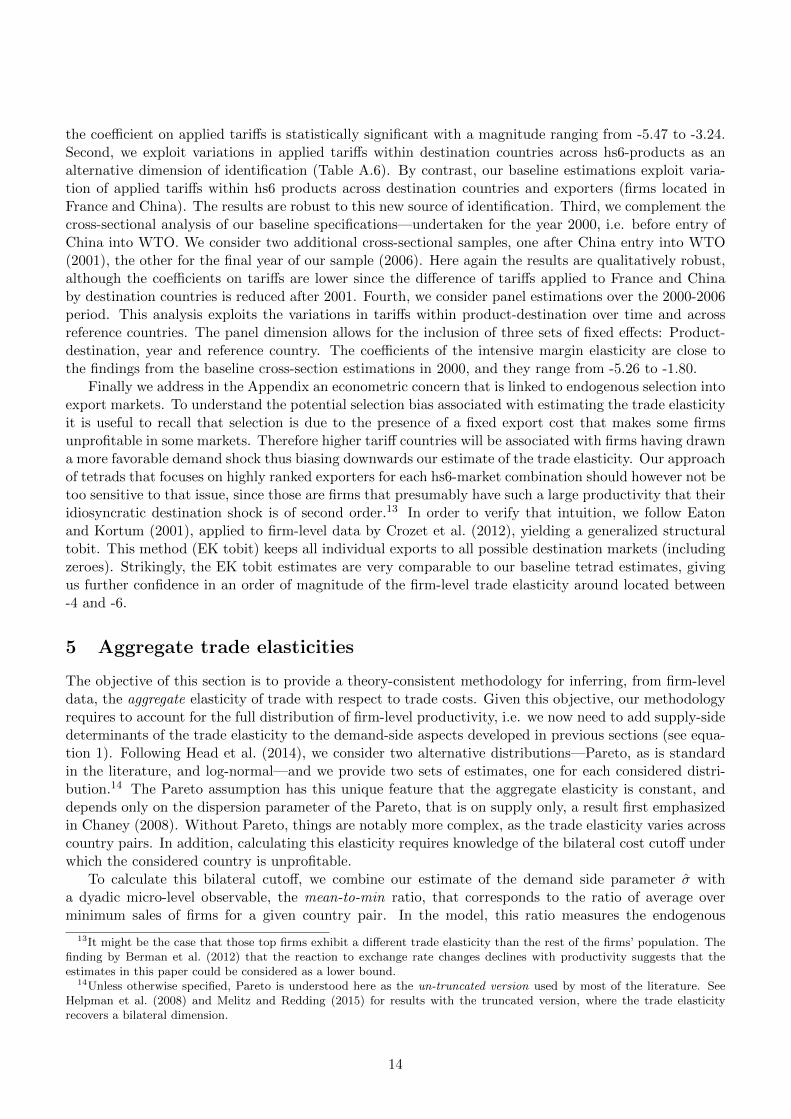
Estimations in Table 1 exploit the variations in tariffs applied to France and China across bothproducts and destination countries. Columns (1) to (3) show the results using as dependent variable theratio of the top 1 exporting French and Chinese firm. Columns (2) presents estimations on the sampleof positive tetraded tariffs and column (3) controls for the tetradic terms of Regional Trade Agreements(RTA). Columns (4) to (6) of Table 1 present the estimations using as dependent variable the ratio offirm-level exports of the top 1 to the top 10 French and Chinese firms. These estimations yield coefficientsfor the applied tariffs (1−σ) that range between -5.74 and -2.66. Note that in both cases, the coefficientson applied tariffs are reduced when including the RTA as expected, but that the tariff variable retainsstatistical significance, showing that the effect of tariffs is not restricted to the binary impact of goingfrom positive to zero tariffs.

In Table 2 we focus on the variations in tariffs within product across destination countries. Thus, allspecifications in this table include (hs6-product × reference country) fixed effects. The coefficients forthe applied tariffs (1− σ) range from -6 and -3.2 for the pair of the Top 1 exporting French and Chinesefirms (columns (1) to (3)). In the extended sample, applied tariffs vary from -4.1 to -1.65. While RTAhas a positive and significant effect, it again does not capture the whole effect of tariff variations acrossdestination countries on export flows. Note also that distance and contiguity have the usual (expected)signs and exhibit very high significance, while the presence of a colonial link and of a common languagehas a much more volatile influence.

In Appendix A.1.2. we present a number of alternative specifications of the intensive margin esti-mates. First we restrict the sample to destination countries applying non-MFN tariffs to France andChina. (Australia, Canada, Japan, New Zealand and Poland) Table A.5 displays the results, where

11

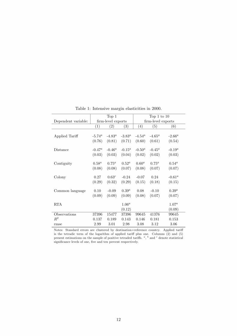
Table 1: Intensive margin elasticities in 2000.

Top 1 Top 1 to 10Dependent variable: firm-level exports firm-level exports

(1) (2) (3) (4) (5) (6)

Applied Tariff -5.74a -4.83a -3.83a -4.54a -4.65a -2.66a

(0.76) (0.81) (0.71) (0.60) (0.61) (0.54)

Distance -0.47a -0.46a -0.15a -0.50a -0.45a -0.19a

(0.03) (0.03) (0.04) (0.02) (0.02) (0.03)

Contiguity 0.58a 0.75a 0.52a 0.60a 0.75a 0.54a

(0.08) (0.08) (0.07) (0.08) (0.07) (0.07)

Colony 0.27 0.63c -0.24 -0.07 0.24 -0.61a

(0.29) (0.32) (0.29) (0.15) (0.18) (0.15)

Common language 0.10 -0.09 0.39a 0.08 -0.10 0.39a

(0.09) (0.09) (0.09) (0.08) (0.07) (0.07)

RTA 1.06a 1.07a

(0.12) (0.09)

Observations 37396 15477 37396 99645 41376 99645R2 0.137 0.189 0.143 0.146 0.181 0.153rmse 2.99 3.01 2.98 3.08 3.12 3.06

Notes: Standard errors are clustered by destination×reference country. Applied tariffis the tetradic term of the logarithm of applied tariff plus one. Columns (2) and (5)present estimations on the sample of positive tetraded tariffs. a, b and c denote statisticalsignificance levels of one, five and ten percent respectively.

12

Table 2: Intensive margin elasticities in 2000. Within-product estimations.


(1) (2) (3) (4) (5) (6)

Applied Tariff -5.99a -5.47a -3.20a -4.07a -3.09a -1.65b

(0.79) (1.07) (0.79) (0.72) (0.75) (0.68)

Distance -0.54a -0.49a -0.21a -0.59a -0.55a -0.29a

(0.03) (0.03) (0.04) (0.03) (0.03) (0.03)


(0.08) (0.09) (0.07) (0.07) (0.09) (0.07)

Colony 0.56a 0.48c 0.01 0.13 0.18 -0.34a

(0.21) (0.29) (0.21) (0.10) (0.15) (0.11)

Common language -0.03 -0.00 0.25a -0.07 -0.07 0.18a

(0.07) (0.08) (0.06) (0.06) (0.07) (0.06)

RTA 1.08a 0.94a

(0.11) (0.07)


Notes: Standard errors are clustered by destination×reference country. All estimationsinclude (hs6-product×reference country) fixed effects. Applied tariff is the tetradic termof the logarithm of applied tariff plus one. Columns (2) and (5) present estimations on thesample of positive tetraded tariffs. a, b and c denote statistical significance levels of one,five and ten percent respectively.

13

the coefficient on applied tariffs is statistically significant with a magnitude ranging from -5.47 to -3.24.Second, we exploit variations in applied tariffs within destination countries across hs6-products as analternative dimension of identification (Table A.6). By contrast, our baseline estimations exploit varia-tion of applied tariffs within hs6 products across destination countries and exporters (firms located inFrance and China). The results are robust to this new source of identification. Third, we complement thecross-sectional analysis of our baseline specifications—undertaken for the year 2000, i.e. before entry ofChina into WTO. We consider two additional cross-sectional samples, one after China entry into WTO(2001), the other for the final year of our sample (2006). Here again the results are qualitatively robust,although the coefficients on tariffs are lower since the difference of tariffs applied to France and Chinaby destination countries is reduced after 2001. Fourth, we consider panel estimations over the 2000-2006period. This analysis exploits the variations in tariffs within product-destination over time and acrossreference countries. The panel dimension allows for the inclusion of three sets of fixed effects: Product-destination, year and reference country. The coefficients of the intensive margin elasticity are close tothe findings from the baseline cross-section estimations in 2000, and they range from -5.26 to -1.80.

Finally we address in the Appendix an econometric concern that is linked to endogenous selection intoexport markets. To understand the potential selection bias associated with estimating the trade elasticityit is useful to recall that selection is due to the presence of a fixed export cost that makes some firmsunprofitable in some markets. Therefore higher tariff countries will be associated with firms having drawna more favorable demand shock thus biasing downwards our estimate of the trade elasticity. Our approachof tetrads that focuses on highly ranked exporters for each hs6-market combination should however not betoo sensitive to that issue, since those are firms that presumably have such a large productivity that theiridiosyncratic destination shock is of second order.13 In order to verify that intuition, we follow Eatonand Kortum (2001), applied to firm-level data by Crozet et al. (2012), yielding a generalized structuraltobit. This method (EK tobit) keeps all individual exports to all possible destination markets (includingzeroes). Strikingly, the EK tobit estimates are very comparable to our baseline tetrad estimates, givingus further confidence in an order of magnitude of the firm-level trade elasticity around located between-4 and -6.

5 Aggregate trade elasticities

The objective of this section is to provide a theory-consistent methodology for inferring, from firm-leveldata, the aggregate elasticity of trade with respect to trade costs. Given this objective, our methodologyrequires to account for the full distribution of firm-level productivity, i.e. we now need to add supply-sidedeterminants of the trade elasticity to the demand-side aspects developed in previous sections (see equa-tion 1). Following Head et al. (2014), we consider two alternative distributions—Pareto, as is standardin the literature, and log-normal—and we provide two sets of estimates, one for each considered distri-bution.14 The Pareto assumption has this unique feature that the aggregate elasticity is constant, anddepends only on the dispersion parameter of the Pareto, that is on supply only, a result first emphasizedin Chaney (2008). Without Pareto, things are notably more complex, as the trade elasticity varies acrosscountry pairs. In addition, calculating this elasticity requires knowledge of the bilateral cost cutoff underwhich the considered country is unprofitable.

To calculate this bilateral cutoff, we combine our estimate of the demand side parameter σ witha dyadic micro-level observable, the mean-to-min ratio, that corresponds to the ratio of average overminimum sales of firms for a given country pair. In the model, this ratio measures the endogenous

13It might be the case that those top firms exhibit a different trade elasticity than the rest of the firms’ population. Thefinding by Berman et al. (2012) that the reaction to exchange rate changes declines with productivity suggests that theestimates in this paper could be considered as a lower bound.

14Unless otherwise specified, Pareto is understood here as the un-truncated version used by most of the literature. SeeHelpman et al. (2008) and Melitz and Redding (2015) for results with the truncated version, where the trade elasticityrecovers a bilateral dimension.

14

dispersion of cross-firm performance on a market, and more precisely the relative performance of entrantsin this market following a change in our variable of interest: variable trade costs.

Under Pareto, the mean-to-min ratio, for a given origin, should be constant and independent ofthe size of the destination market. This pattern of scale-invariance is not observed in the data wherewe see that mean-to-min ratios increase massively in large markets—a feature consistent with a log-normal distribution of firm-level productivity. In the last step of the section we compare our micro-basedpredicted elasticities to those estimated with a gravity-like approach based on macro-data.

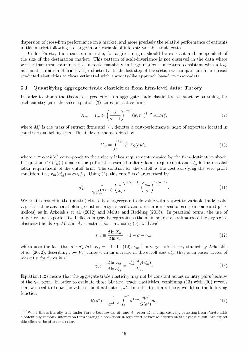
5.1 Quantifying aggregate trade elasticities from firm-level data: Theory

In order to obtain the theoretical predictions on aggregate trade elasticities, we start by summing, foreach country pair, the sales equation (2) across all active firms:

Xni = Vni ×(

σ

σ − 1

)1−σ(wiτni)

1−σ AnMei , (9)

where M ei is the mass of entrant firms and Vni denotes a cost-performance index of exporters located in

country i and selling in n. This index is characterized by

Vni ≡∫ a∗ni

0a1−σg(a)da, (10)

where a ≡ α× b(α) corresponds to the unitary labor requirement rescaled by the firm-destination shock.In equation (10), g(.) denotes the pdf of the rescaled unitary labor requirement and a∗ni is the rescaledlabor requirement of the cutoff firm. The solution for the cutoff is the cost satisfying the zero profitcondition, i.e., xni(a

∗ni) = σwifni. Using (2), this cutoff is characterized by

a∗ni =1

τnif1/(σ−1)ni

(1

wi

)σ/(σ−1)(Anσ

)1/(σ−1). (11)

We are interested in the (partial) elasticity of aggregate trade value with-respect to variable trade costs,τni. Partial means here holding constant origin-specific and destination-specific terms (income and priceindices) as in Arkolakis et al. (2012) and Melitz and Redding (2015). In practical terms, the use ofimporter and exporter fixed effects in gravity regressions (the main source of estimates of the aggregateelasticity) holds wi, Mi and An constant, so that, using (9), we have15

εni ≡d lnXni

d ln τni= 1− σ − γni, (12)

which uses the fact that d ln a∗ni/d ln τni = −1. In (12), γni is a very useful term, studied by Arkolakiset al. (2012), describing how Vni varies with an increase in the cutoff cost a∗ni, that is an easier access ofmarket n for firms in i:

γni ≡d lnVnid ln a∗ni

=a∗2−σni g(a∗ni)

Vni. (13)

Equation (12) means that the aggregate trade elasticity may not be constant across country pairs becauseof the γni term. In order to evaluate those bilateral trade elasticities, combining (13) with (10) revealsthat we need to know the value of bilateral cutoffs a∗. In order to obtain those, we define the followingfunction

H(a∗) ≡ 1

a∗1−σ

∫ a∗

0a1−σ

g(a)

G(a∗)da, (14)

15While this is literally true under Pareto because wi, Mi and An enter a∗ni multiplicatively, deviating from Pareto addsa potentially complex interaction term through a non-linear in logs effect of monadic terms on the dyadic cutoff. We expectthis effect to be of second order.

15

a monotonic, invertible function which has a straightforward economic interpretation in this model. It isthe ratio of average over minimum performance (measured as a∗1−σ) of firms located in i and exportingto n. Using equations (2) and (9), this ratio also corresponds to the observed mean-to-min ratio of sales:

xnixni(a∗ni)

= H(a∗ni). (15)

For our two origin countries (France and China), we observe the ratio of average to minimum trade flowsfor each destination country n. Using equation (15), one can calibrate a∗nFR and a∗nCN, the estimatedvalue of the export cutoff for French and Chinese firms exporting to n as a function of the mean-to-minratio of French and Chinese sales on each destination market n

a∗nFR = H−1(xnFRxMINnFR

), and a∗nCN = H−1

(xnCN

xMINnCN

). (16)

Equipped with the dyadic cutoffs we use equations (12) to (15) to obtain the aggregate trade elasticities

εnFR = 1− σ −xMINnFR

xn,FR×a∗nFRg(a∗nFR)

G(a∗nFR), and εnCN = 1− σ −

xMINnCN

xnCN×a∗nCNg(a∗nCN)

G(a∗nCN), (17)

where σ is our estimate of the intensive margin (the demand-side parameter) from previous sections.Our inference procedure is characterized by equations (16), and (17). We also calculate two other trademargins: the elasticity of the number of active exporters Nni (the so-called extensive margin) and theelasticity of average shipments xni. The number of active firms is closely related to the cutoff sinceNni = M e

i ×G(a∗ni), where M ei represents the mass of entrants (also absorbed by exporter fixed effects in

gravity regressions). Differentiating the previous relationship and using (17) we can estimate the dyadicextensive margin of trade

d lnNnFR

d ln τnFR= −

a∗nFRg(a∗nFR)

G(a∗nFR), and

d lnNnCN

d ln τnCN= −

a∗nCNg(a∗nCN)

G(a∗nCN), (18)

From the accounting identity Xni ≡ Nni × xni, we obtain the (partial) elasticity of average shipmentsto trade simply as the difference between the estimated aggregate elasticities, (17) and the estimatedextensive margins, (18).

d ln xnFRd ln τnFR

= εnFR −d lnNnFR

d ln τnFRand

d ln xnCN

d ln τnCN= εnCN −

d lnNnCN

d ln τnCN, (19)

For the sake of interpreting the role of the mean-to-min, we combine (17) and (18) to obtain a relationshiplinking the aggregate elasticities to the (intensive and extensive) margins and to the mean-to-min ratio.Taking France as an origin country for instance, we obtain:

εnFR = 1− σ︸︷︷︸intensive margin

+1

xnFR/xMINnFR︸︷︷︸min-to-mean

× d lnNnFR

d ln τnFR︸︷︷︸extensive margin

, (20)

which is equation (1) presented in the introduction. This decomposition shows that the aggregate tradeelasticity is the sum of the intensive margin and of the (weighted) extensive margin. The weight onthe extensive margin depends only on the mean-to-min ratio, an observable measuring the dispersionof relative firm performance. Intuitively, the weight of the extensive margin should be decreasing whenthe market gets easier. Indeed easy markets have larger rates of entry, G(a∗), and therefore increasingpresence of weaker firms which augments dispersion measured as H(a∗ni). The marginal entrant in an easymarket will therefore have less of an influence on aggregate exports, a smaller impact of the extensivemargin. In the limit, the weight of the extensive margin becomes negligible and the whole of the aggregateelasticity is due to the intensive margin / demand parameter. In the Pareto case however this mechanismis not operational since H(a∗ni) and therefore the weight of the extensive margin is constant. We now turnto implementing our method with Pareto as opposed to an alternative distribution yielding non-constantdispersion of sales across destinations.

16

5.2 Quantifying aggregate trade elasticities from firm-level data: Results

A crucial step for our quantification procedure consists in specifying the distribution of rescaled laborrequirement, G(a), which is necessary to inverse the H function, reveal the bilateral cutoffs and obtain thebilateral trade elasticities. The literature has almost exclusively used the Pareto. Head et al. (2014) showthat a credible alternative, which seems favored by firm-level export data, is the log-normal distribution.Pareto-distributed rescaled productivity ϕ ≡ 1/a translates into a power law CDF for a, with shapeparameter θ. A log-normal distribution of a retains the log-normality of productivity (with locationparameter µ and dispersion parameter ν) but with a change in the log-mean parameter from µ to −µ.The CDFs for a are therefore given by

GP(a) =(aa

)θ, and GLN(a) = Φ

(ln a+ µ

ν

), (21)

where we use Φ to denote the CDF of the standard normal. Simple calculations using (21) in (14), anddetailed in Appendix 2:, show that the resulting formulas for H are

HP(a∗ni) =θ

θ − σ + 1, and HLN(a∗ni) =

h[(ln a∗ni + µ)/ν]

h[(ln a∗ni + µ)/ν + (σ − 1)ν], (22)

where h(x) ≡ φ(x)/Φ(x), the ratio of the PDF to the CDF of the standard normal.Calculating GP(.), GLN(.), HP(.) and HLN(.) requires knowledge of underlying key supply-side distri-

bution parameters θ and ν. For those, we use estimates from the Quantile-Quantile (QQ) regressions inHead et al. (2014). This method, based on a regression of empirical against theoretical quantiles of logsales, is applied on the same samples of exporters (Chinese and French) as here, and requires an estimateof the CES. We choose σ = 5, which corresponds to a central value in our findings on the intensive marginabove (where the average value of 1− σ ' −4).

Panel (a) of Figure 4 depicts the theoretical relationship between the ratio of average to minimumsales, H(a∗ni), and the probability of serving the destination market , G(a∗ni), spanning over values of thecutoff a∗ni. Under Pareto heterogeneity, H is constant but this property of scale invariance is specific tothe Pareto: Indeed it is increasing in G under log-normal. Panel (b) of figure 4 depicts the empiricalcounterpart of this relationship as observed for French and Chinese exporters in 2000 for all countries inthe world. On the x-axis is the share of exporters serving each of those markets.16 Immediately apparentis the non-constant nature of the mean-to-min ratio in the data, contradicting the Pareto prediction.This finding is very robust when considering alternatives to the minimum sales (which might be noisy ifonly because of statistical threshold effects) for the denominator of H, that is different quantiles of theexport distribution.17

16While this is not exactly the empirical counterpart of G(a∗ni), the x-axis of panel (a), those two shares differ by amultiplicative constant, leaving the shape of the (logged) relationship unchanged.

17In a further effort to minimize noise in the calculation of the mean-to-min ratio, the figures are calculated for each ofthe 99 HS2 product categories and averaged. In the rest of the section, we will stick with this approach for the calculationof elasticities, done at the sector level before being averaged, which also simplifies exposition.

17

Figure 4: Theoretical and Empirical Mean-to-Min ratios

Pareto (FRA): 4.52

Pareto (CHN): 2.62

Log-normal

110

100

1000

1000

0H

.001 .01 .1 .2 .5 1Probability of serving market

French exportersChinese exporters

Pareto (FRA): 4.52

Pareto (CHN): 2.62

110

100

1000

1000

0ra

tio o

f mea

n to

min

sal

es.001 .01 .1 .2 .5 1

share of exporters


(a) theory (b) data

Figure 5 turns to the predicted trade elasticities under the two alternative distributions. Functionalforms from (21) and (22) into (17), are used to deliver the two aggregate elasticities εPni and εLNni :

εPni = −θ, and εLNni = 1− σ − 1

νh

(ln a∗ni + µ

ν+ (σ − 1)ν

). (23)

Parallel to figure 4, panel (a) of figure 5 shows the theoretical relationship between those elasticitiesand G(a∗ni), while panel (b) plots the same elasticities evaluated for each individual destination countryagainst the empirical counterpart of G(). Again, the Pareto case has a constant prediction (one for eachexporter), while log normal predicts a trade elasticity that is declining (in absolute value) with easiness ofthe market. Panel (b) confirms the large variance of trade elasticities according to the share of exportersthat are active in each of the markets. It also shows that the response of aggregate flows to trade costsis reduced (in absolute value) when the market becomes easier. The intuition is that for very difficultmarkets, the individual reaction of incumbent firms is supplemented with entry of exporters selectedamong the most efficient firms. The latter effect becomes negligible for the easiest markets, yielding ε toapproach the intensive margin. This mechanism becomes very clear when looking at the patterns of theextensive margin and average export elasticities in figure 6.

The predicted elasticity on the extensive margin is also rising with market toughness as shown inpanel (a) of figure 6. The inverse relationship is true for average exports (panel b). When a marketis very easy and most exporters make it there, the extensive margin goes to zero, and the response ofaverage exports goes to the value of the intensive margin (the firm-level response), 1 − σ, as shown infigure 6 when the share of exporters increase. While this should intuitively be true in general, Paretodoes not allow for this change in elasticities across markets, since the response of average exports shouldbe uniformly 0, while the total response is entirely due to the (constant) extensive margin. In Table3, we compute the average value and standard deviation of bilateral trade elasticities calculated usinglog-normal, and presented in figures 5 and 6. The first column presents the statistics for the Frenchexporters’ sample, the second one is the Chinese exporters’ case, and the last column averages those.The mean elasticities obtained vary slightly between France and China, but the dominant feature is thatthe total elasticity is in neither case confined to the extensive margin. In both cases, average exports arepredicted to react strongly to trade costs, a pattern we will confirm on actual data in the next subsection.

18

Figure 5: Predicted trade elasticities: εnFR and εnCN

Pareto (FRA): ε = -θ = -5.13

Pareto (CHN): ε = -θ = -6.47

Log-normal

-9-8

-7-6

-5-4

Trad

e El

astic

ity: ε

.001 .01 .1 .2 .5 1Probability of serving market


Pareto (FRA): ε = -θ = -5.13

Pareto (CHN): ε = -θ = -6.47

Log-normal

-9-8

-7-6

-5-4

Trad

e el

astic

ity: ε

.001 .01 .1 .2 .5 1Share of exporters


(a) theory (b) data

Figure 6: Predicted elasticities: extensive and average exports

Pareto (FRA): ε = -θ = -5.13

Pareto (CHN): ε = -θ = -6.47

Log-normal

-9-8

-7-6

-5-4

-3-2

-10

Num

ber o

f exp

orte

rs e

last

icity



Pareto

Log-normal

-4-3

-2-1

0Av

erag

e ex

ports

ela

stic

ity



(a) extensive margin (b) average exports

19

Table 3: Predicted bilateral trade elasticities (LN distribution)

LHS France China Average

Total flows -5.14 -4.792 -4.966(1.069) (.788) (.742)

Number of exporters -2.866 -2.274 -2.57(1.657) (1.472) (1.335)

Average flows -2.274 -2.517 -2.396(.687) (.731) (.64)

Notes: This table presents the predicted elasticities (mean ands.d.) on total exports, the number of exporting firms, and av-erage export flows. Required parameters are σ, the CES, andν, the dispersion parameter of the log normal distribution.

Figure 7 groups our bilateral trade elasticities (εni) into ten bins of export shares for both France andChina in a way similar to empirical evidence by Novy (2013), which reports that the aggregate trade costelasticity decreases with bilateral trade intensity.18 The qualitative pattern is very similar here, with thebilateral elasticity decreasing in absolute value with the share of exports going to a destination. One canuse this variance in εni to quantify the error that a practitioner would make when assuming a constantresponse of exports to a trade liberalization episode. Taking China as an example, decreasing trade costsby one percent would raise flows by around 6.5 percent for countries like Somalia, Chad or Azerbaijan(first bin of Chinese exports) and slightly more than 4 percent for the USA and Japan (top bin). Sincethe estimate that would be obtained when imposing a unique elasticity would be close to the averageelasticity (4.79), this would entail about 25 percent underestimate of the trade growth for initially lowtraders (1.7/6.5) and an overestimate of around 20 percent (.8/4) for the top trade pairs.19

18Although Novy (2013) estimates variable distance elasticity, his section 3.4 assumes a constant trade costs to distanceparameter to focus on the equivalent of our εni.

19We thank Steve Redding for suggesting this quantification.

20

Figure 7: Variance in trade elasticities: εnFR and εnCN

average elasticity: 5.14

45

67

8Tr

ade

Elas

ticity

: -ε

1 2 3 4 5 6 7 8 9 10Export share bin

average elasticity: 4.79

45

67

8Tr

ade

Elas

ticity

: -ε

1 2 3 4 5 6 7 8 9 10Export share bin

(a) French exports (b) Chinese exports

5.3 Comparison with macro-based estimates of trade elasticities

We now can turn to empirical estimates of aggregate elasticities to be compared with our predictions.Those are obtained using aggregate versions of our estimating tetrad equations presented above, which isvery comparable to the method most often used in the literature: a gravity equation with country fixedeffects and a set of bilateral trade costs covariates, on which a constant trade elasticity is assumed.20

Column (1) of Table 4 uses the same sample of product-markets as in our benchmark firm-level estimationsand runs the regression on the tetrad of aggregate rather than individual exports. Column (2) uses thesame covariates but on the count of exporters, and column (3) completes the estimation by looking atthe effects on average flows. An important finding is that the effect on average trade flow is estimatedat -2.55, and is significant at the 1% level, contrary to the Pareto prediction (in which no variable tradecost should enter the equation for average flows).21 This finding is robust to controlling for RTA (column6) or constraining the sample to positive tariffs (column 9). The estimated median trade elasticity ontotal flows over all specifications at -4.79, is very close from the -5.03 found as the median estimate inthe literature by Head and Mayer (2014).

Under Pareto, the aggregate elasticity should reflect fully the one on the number of exporters, andthere should be no impact of tariffs on average exports. This prediction of the Pareto distribution istherefore strongly contradicted by our results. As a first pass at assessing whether, the data support thelog-normal predictions, we compare the (unique) macro-based elasticity obtained in Table 4, with thecorresponding average of bilateral elasticities shown in Table 3 of the preceding sub-section. The numbersobtained are quite comparable when the effects of RTAs are taken into account (columns (4) to (6)) or with

20Note that the gravity prediction on aggregate flows where origin, destination, and bilateral variables are multiplicativelyseparable and where there is a unique trade elasticity is only valid under Pareto. The heterogeneous elasticities generated bydeviating from Pareto invalidate the usual gravity specification. Our intuition however is that the elasticity estimated usinggravity/tetrads should be a reasonable approximation of the average bilateral elasticities. In order to verify this intuition,we run Monte Carlo simulations of the model with log-normal heterogeneity and find that indeed the average of micro-basedheterogeneous elasticities is very close to the unique macro-based estimate in a gravity/tetrads equation on aggregate flows.Description of those simulations are in Appendix 3:.

21Note that the three dependent variables are computed for each hs6 product-destination, and therefore that the averageexports do not contain an extensive margin where number of products would vary across destinations.

21

Table 4: Elasticites of total flows, count of exporters and average trade flows.

Tot. # exp. Avg. Tot. # exp. Avg. Tot. # exp. Avg.(1) (2) (3) (4) (5) (6) (7) (8) (9)

Applied Tariff -6.84a -4.29a -2.55a -4.00a -1.60b -2.41a -4.79a -2.13a -2.66a

(0.82) (0.66) (0.54) (0.73) (0.63) (0.50) (0.84) (0.50) (0.54)

Distance -0.85a -0.61a -0.24a -0.51a -0.28a -0.23a -0.85a -0.60a -0.25a

(0.04) (0.03) (0.02) (0.05) (0.03) (0.03) (0.04) (0.03) (0.02)

Contiguity 0.62a 0.30a 0.32a 0.53a 0.21a 0.32a 0.64a 0.35a 0.29a

(0.12) (0.09) (0.06) (0.11) (0.07) (0.05) (0.12) (0.09) (0.06)

Colony 0.93a 0.72a 0.20a 0.38a 0.20b 0.17b 1.12a 0.94a 0.17b

(0.11) (0.10) (0.06) (0.13) (0.10) (0.08) (0.14) (0.11) (0.07)

Common language 0.09 0.16c -0.07 0.39a 0.44a -0.05 -0.02 0.05 -0.07(0.09) (0.09) (0.06) (0.09) (0.08) (0.06) (0.10) (0.08) (0.06)

RTA 1.10a 1.04a 0.06(0.11) (0.06) (0.07)

Observations 99645 99645 99645 99645 99645 99645 41376 41376 41376R2 0.319 0.537 0.063 0.331 0.575 0.063 0.311 0.505 0.066rmse 1.79 0.79 1.47 1.77 0.76 1.47 1.65 0.75 1.34

Notes: All estimations include fixed effects for each product-reference importer country combination. Standarderrors are clustered at the destination-reference importer level. The dependent variable is the tetradic term of thelogarithm of total exports at the hs6-destination-origin country level in columns (1), (4) and (7); of the number ofexporting firms by hs6-destination and origin country in columns (2), (5) and (8) and of the average exports at thehs6-destination-origin country level in columns (3), (6) and (9). Applied tariff is the tetradic term of the logarithmof applied tariff plus one. Columns (7) to (9) present the estimations on the sample of positive tetraded tariffs andnon-MFN tariffs. a, b and c denote statistical significance levels of one, five and ten percent respectively.

22

positive tetrad tariffs (columns (7) to (9)). Although this is not a definitive validation of the heterogenousfirms model with log-normal distribution, our results clearly favor this distributional assumption overPareto, and provides support for the empirical relevance of non-constant trade elasticities.

5.4 Direct evidence of non-constant trade elasticities

We can further use tetrads on aggregate trade flows in order to show direct empirical evidence of non-constant trade elasticities. Using aggregate bilateral flows from equation (9), and building tetrads witha procedure identical to the one used in Section 2.2, we obtain the (FR,CN, n, k)–tetrad of aggregateexports

X{n,k} ≡XnFR/XkFR

XnCN/XkCN=

(τnFR/τkFRτnCN/τkCN

)1−σ

× VnFR/VkFRVnCN/VkCN

(24)

Taking logs, differentiating with respect to tariffs and using the expression for the cutoff (11), we obtain

d ln X{n,k} = (1− σ − γnFR)× d ln τnFR − (1− σ − γkFR)× d ln τkFR

− (1− σ − γnCN)× d ln τnCN + (1− σ − γkCN)× d ln τkCN, (25)

where γni is the elasticity of the cost performance index to a rise in the easiness of the market, defined in(13). For general distributions of heterogeneity, this elasticity is not constant across dyads as it dependson the dyad-specific cutoff a∗ni. Hence, our interpretation of equation (25) is that the contribution to the(tetraded) total exports of a change in bilateral tariffs is larger for dyads that have a larger elasticity.Under Pareto, this elasticity is constant across dyads, γPni = 1−σ+ θ. Combined with equation (25) thisleads to

εP{n,k} =d ln X{n,k}

d ln τ{n,k}= −θ, (26)

where τ{n,k} is the vector of tetraded trade costs. This formula states that under Pareto, the elasticityof tetrad exports to tetrad tariffs is equal to the supply-side parameter θ. This transposes to the tetradenvironment the well-known result of Chaney (2008) on gravity. Under non-Pareto heterogeneity, thefour elasticities in (25) will remain different, a prediction we can put to a test. Results are shown in Table5, where we pool observations for the years 2000 to 2006. Columns (1), (2) and (3) are the equivalentof the first three columns in Table 4, with the trade costs tetrads being split into its four componentsand the coefficients allowed to differ. The coefficients on tariffs to the destination country n show thatthe elasticity when considering France and China as an origin country differ significantly, consistentwith the non-Pareto version of heterogeneity. Coefficients related to the reference importer k also differsignificantly from each other, supporting further heterogeneity in the trade elasticities. A related approachis to confine identification on the destination country, neutralizing the change of reference country witha k fixed effect. Those results are shown in columns (4) to (6), where again most of the tariff elasticitiesdiffer across origin countries.22

22Table A.12 shows those same estimations for the two extreme years of our sample, 2000 and 2006, with significantevidence of non-constant elasticities in most cases.

23

Table 5: Non-constant trade elasticity

Dependent variable: Tot. # exp. Avg. Tot. # exp. Avg.

(1) (2) (3) (4) (5) (6)

Applied Tariffn,FR -4.25a -2.90a -1.34a -4.06a -2.76a -1.30a

(0.27) (0.25) (0.18) (0.26) (0.23) (0.17)

Applied Tariffn,CN 3.43a 1.87a 1.56a 3.30a 1.76a 1.53a

(0.27) (0.25) (0.17) (0.26) (0.23) (0.17)

Applied Tariffk,FR 7.11a 6.60a 0.52b

(0.36) (0.20) (0.24)

Applied Tariffk,CN -3.79a -2.14a -1.66a

(0.40) (0.26) (0.23)


Notes: All estimations include a product and year fixed effects and the four components (n,FR;n,CN; k,FR; and k,CN) of each gravity control (distance, common language, contiguity andcolony). In all estimations standard errors are clustered at the destination-reference country andyear level.

5.5 Micro and Aggregate elasticities at the industry level

As a last exercise, we provide evidence that both demand and supply determinants enter the aggregateelasticity by looking at industry-level estimates. For each good, we can estimate a firm-level and anaggregate elasticity to tariffs (as in sections 4.2 and 5.3 respectively). Under the Pareto assumption,those two elasticities have no reason to be correlated, since the micro elasticity is a measure of productdifferentiation, while the macro one is capturing homogeneity in firms’ productive efficiency. Underalternative distributions like the log-normal, the aggregate elasticity includes both determinants andtherefore should be correlated with the micro one (equation 1).

We run our micro and macro-level tetrad estimations for each 2-digit ISIC industry separately includ-ing destination-reference country and year fixed effects. Table 6 presents the results. Columns (1) and(2) show the coefficients for the micro-level elasticity while columns (3) and (4) report the estimates ofthe aggregate elasticity using the tetrad term of total exports by product-destination-reference countryand year. Columns (2) and (4) restrict the sample to EU destinations. Each cell reports the coefficienton the applied tariffs tetrad by industry with associated degree of statistical significance.

Estimates at the industry level yield coefficients of the intensive margin elasticity that average to-2.67 (column 1). The coefficients of the aggregate elasticity have a mean of -3.22 (column 3). Moreimportant for our main investigation, the intensive and aggregate elasticities are correlated (pairwisecorrelations are .68 for the full sample, and .74 for the EU one). Figure 8 shows graphical evidenceof those correlations that exhibits overwhelming evidence in favor of the aggregate elasticity includingdemand side determinants.

24

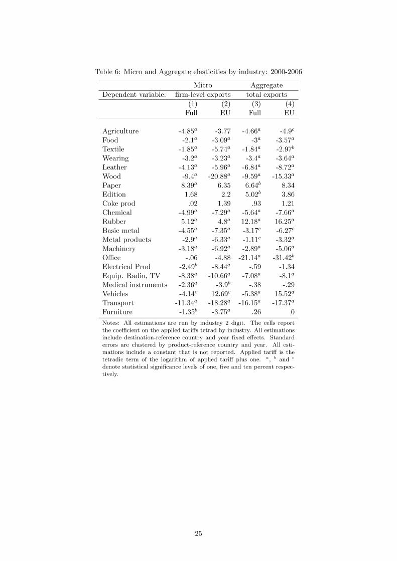
Table 6: Micro and Aggregate elasticities by industry: 2000-2006

Micro Aggregate

Dependent variable: firm-level exports total exports

(1) (2) (3) (4)Full EU Full EU

Agriculture -4.85a -3.77 -4.66a -4.9c

Food -2.1a -3.09a -3a -3.57a

Textile -1.85a -5.74a -1.84a -2.97b

Wearing -3.2a -3.23a -3.4a -3.64a

Leather -4.13a -5.96a -6.84a -8.72a

Wood -9.4a -20.88a -9.59a -15.33a

Paper 8.39a 6.35 6.64b 8.34Edition 1.68 2.2 5.02b 3.86Coke prod .02 1.39 .93 1.21Chemical -4.99a -7.29a -5.64a -7.66a

Rubber 5.12a 4.8a 12.18a 16.25a

Basic metal -4.55a -7.35a -3.17c -6.27c

Metal products -2.9a -6.33a -1.11c -3.32a

Machinery -3.18a -6.92a -2.89a -5.06a

Office -.06 -4.88 -21.14a -31.42b

Electrical Prod -2.49b -8.44a -.59 -1.34Equip. Radio, TV -8.38a -10.66a -7.08a -8.1a

Medical instruments -2.36a -3.9b -.38 -.29Vehicles -4.14c 12.69c -5.38a 15.52a

Transport -11.34a -18.28a -16.15a -17.37a

Furniture -1.35b -3.75a .26 0

Notes: All estimations are run by industry 2 digit. The cells reportthe coefficient on the applied tariffs tetrad by industry. All estimationsinclude destination-reference country and year fixed effects. Standarderrors are clustered by product-reference country and year. All esti-mations include a constant that is not reported. Applied tariff is thetetradic term of the logarithm of applied tariff plus one. a, b and c

denote statistical significance levels of one, five and ten percent respec-tively.

25

Figure 8: Aggregate and intensive margin elasticities by industry 2 digit

Agriculture

FoodTextile

WearingLeather

Wood

Paper

Edition

Coke prod

Chemical

Rubber

Basic metal

Metal productsMachinery

Office

Electrical Prod

Equip. Radio, TV

Medical instruments

Vehicles

Transport

Furniture

-15

-10

-50

510

15M

icro

ela

stic

ity (

1-s)

-30 -20 -10 0 10Aggregate elasticity (e)

Agriculture

FoodTextile

Wearing

Leather

Wood

ChemicalBasic metal

Metal productsMachinery

Equip. Radio, TV

Vehicles

Transport

-15

-10

-50

Mic

ro e

last

icity

(1-

s)

-20 -15 -10 -5 0Aggregate elasticity (e)

(a) Full set (b) Coeff sig. < 0

6 Conclusion

We have argued in this paper that knowledge of the firm-level response to trade costs is a central elementto our understanding of aggregate export reaction. In other words, we need micro-level data to understandthe macro-level impacts of trade costs, a central element in any trade policy evaluation. This need formicro data is presumably true with the vast majority of possible heterogeneity distribution assumptions.There is one exception however where micro data is not needed to estimate the aggregate elasticity: the(untruncated) Pareto distribution. It is an exception the literature has been concentrating on for reasonsof tractability that are perfectly legitimate, but the evidence presented in our paper points to systematicvariation in bilateral aggregate trade elasticities that is both substantial and compatible with log-normalheterogeneity (in addition to be strongly preferred when looking at the micro-level distribution of exportsales). We therefore call for a “micro approach” to estimating those elasticities as opposed to the “macroapproach” using gravity specified so as to estimate a constant elasticity.

The micro- and macro- approaches differ substantially in several respects. On the one hand, gravity isa more direct and parsimonious route for estimating aggregate elasticities: (i) parametric assumptions arereduced to a minimum while our micro-based procedure depends on the calibration of the productivitydistribution; (ii) gravity is less demanding in terms of data and makes possible the use of easily accessibledataset of bilateral aggregate trade flows. On the other hand, gravity provides, for each origin country,only a cross-destination average of elasticities while the micro-based approach provides the full cross-dyadic distribution of elasticities. Given this last limitation, we use our gravity estimates of averagedelasticities as a benchmark for discriminating between the two distributional assumptions made in ourmicro-based quantifications. We find that average value of bilateral trade elasticities obtained under alog-normal calibration is very close to the empirical gravity estimate which constrains the elasticity to beconstant across country pairs. By contrast, the Pareto-based calibration leads to predictions that seeminvalidated by the data. Namely, the invariance of average shipments to ad-valorem tariff variations, thelack of correlation between firm-level and aggregate level of elasticities estimated industry by industry,and the constant aggregate trade elasticities.

26

References

Anderson, J. E. and van Wincoop, E. (2003). Gravity with gravitas: A solution to the border puzzle.American Economic Review, 93 (1):170–192.

Arkolakis, C. (2010). Market penetration costs and the new consumers margin in international trade.Journal of Political Economy, 118(6):1151 – 1199.

Arkolakis, C., Costinot, A., and Rodrıguez-Clare, A. (2010). Gains from trade under monopolisticcompetition: A simple example with translog expenditure functions and pareto distributions of firm-level productivity. manuscript.

Arkolakis, C., Costinot, A., and Rodriguez-Clare, A. (2012). New trade models, same old gains? Amer-ican Economic Review, 102(1):94–130.

Atkeson, A. and Burstein, A. (2008). Pricing-to-market, trade costs, and international relative prices.The American Economic Review, 98(5):1998–2031.

Baier, S. and Bergstrand, J. H. (2001). The growth of world trade: tariffs, transport costs, and incomesimilarity. Journal of International Economics, 53 (1):1–27.

Barba Navaretti, G., Bugamellli, M., Forlani, E., and Ottaviano, G. (2015). It takes (more than) amoment: Revisiting the link between firm productivity and aggregate exports. University of MilanMimeo.

Berman, N., Martin, P., and Mayer, T. (2012). How do different exporters react to exchange rate changes?The Quarterly Journal of Economics, 127 (1):437–492.

Berthou, A. and Fontagne, L. (2015). Variable trade costs, composition effects, and the intensive marginof trade. Technical Report 543, Banque de France.

Broda, C. and Weinstein, D. (2006). Globalization and the gains from variety. Quarterly Journal ofEconomics, 121 (2):541–585.

Caliendo, L. and Parro, F. (2015). Estimates of the trade and welfare effects of nafta. Review of EconomicStudies, 82(1):1–44.

Chaney, T. (2008). Distorted gravity: The intensive and extensive margins of international trade. Amer-ican Economic Review, 98 (4):1707–1721.

Costinot, A., Donaldson, D., and Komunjer, I. (2012). What goods do countries trade? a quantitativeexploration of ricardo’s ideas. Review of Economic Studies, 79(2):581–608.

Crozet, M., Head, K., and Mayer, T. (2012). Quality sorting and trade: Firm-level evidence for frenchwine. Review of Economic Studies, 79(2):609 – 644.

Eaton, J. and Kortum, S. (2001). Trade in capital goods. European Economic Review, 45(7):1195–1235.

Eaton, J. and Kortum, S. (2002). Technology, geography, and trade. Econometrica, 70 (5):1741–1779.

Eaton, J., Kortum, S., and Kramarz, F. (2011). An anatomy of international trade: Evidence fromFrench firms. Econometrica, 79(5):1453–1498.

Feenstra, R. C. (1994). New product varieties and the measurement of international prices. AmericanEconomic Review, 84:157–177.

27

Feenstra, R. C. (2003). A homothetic utility function for monopolistic competition models. EconomicsLetters, 78(2):79–86.

Feenstra, R. C. (2013). Restoring the product variety and pro-competitive gains from trade with hetero-geneous firms and bounded productivity. UC Davis Mimeo.

Fernandes, A., Klenow, P., Meleshchuk, S., Pierola, M. D., and Rodriguez-Clare, U. A. (2015). Theintensive margin puzzle in trade. mimeo.

Fitzgerald, D. and Haller, S. (2014). Exporters and shocks: Dissecting the international elasticity puzzle.manuscript.

Freund, C. and Pierola, M. D. (2015). Export superstars. Review of Economics and Statistics.

Gopinath, G. and Neiman, B. (2014). Trade adjustment and productivity in large crises. AmericanEconomic Review, 104(3):793–831.

Hallak, J. C. (2006). Product quality and the direction of trade. Journal of International Economics, 68(1):238–265.

Head, K. and Mayer, T. (2014). Gravity equations: Workhorse, toolkit, and cookbook. In Helpman, E.,Gopinath, G., and Rogoff, K., editors, Handbook of International Economics, volume 4. Elsevier.

Head, K., Mayer, T., and Ries, J. (2010). The erosion of colonial trade linkages after independence.Journal of International Economics, 81 (1):1–14.

Head, K., Mayer, T., and Thoenig, M. (2014). Welfare and trade without pareto. American EconomicReview, 104(5):310–16.

Head, K. and Ries, J. (2001). Increasing returns versus national product differentiation as an explanationfor the pattern of us-canada trade. American Economic Review, 91(4):858–876.

Helpman, E., Melitz, M., and Rubinstein, Y. (2008). Estimating trade flows: Trading partners andtrading volumes. Quarterly Journal of Economics, 123(2):441–487.

Hummels, D. (1999). Towards a geography of trade costs. Technical Report 17, GTAP Working Paper.

Imbs, J. and Mejean, I. (2015). Elasticity optimism. American Economic Journal: Macroeconomics, 7(3):43–83.

Krugman, P. (1980). Scale economies, product differentiation, and the pattern of trade. AmericanEconomic Review, 70:950–959.

Melitz, M. (2003). The impact of trade on intra-industry reallocations and agregate industry productivity.Econometrica, 71:1695–1725.

Melitz, M. and Ottaviano, G. (2008). Market size, trade, and productivity. Review of Economic Studies,75(1):295–316.

Melitz, M. J. and Redding, S. J. (2015). New trade models, new welfare implications. American EconomicReview.

Novy, D. (2013). International trade without CES: Estimating translog gravity. Journal of InternationalEconomics, 89(2):271–282.

Ossa, R. (2015). Why trade matters after all. Journal of International Economics.

28

Romalis, J. (2007). Nafta’s and cusfta’s impact on international trade. Review of Economics and Statis-tics, 89(3):416 – 435.

Simonovska, I. and Waugh, M. E. (2011). The elasticity of trade: Estimates and evidence. WorkingPaper 16796, NBER.

Yang, M.-J. (2014). Firm heterogeneity and trade in a distorted gravity world. University of WashingtonMimeo.

29

Appendix 1: Empirical Appendix

A.1.1. Descriptive statistics

Table A.1: Average percentage point difference between the applied tariff to France and China acrossindustries by Germany and Japan (2000)

Reference importer: Germany Japan

Full Tetrad Full Tetradsample regression sample sample regression sample

Agriculture -3.27 -2.98 .01 .02Food -7.83 -9.63 1.24 1.45Textile -7.14 -6.95 5.31 4.58Wearing apparel -9.34 -8.11 6.2 6.79Leather -1.5 -1.15 8.4 4.68Wood -1.36 -1.47 2.66 3.69Paper 0 0 1.39 1.3Edition -.79 -.65 .26 .64Coke prod 0 0 .97 1.73Chemical -1.01 -.74 2.51 2.4Rubber & Plastic -1.37 -1.25 2.5 2.37Non Metallic -1.43 -2.18 1.16 .8Basic metal products -1.84 -3.56 1.89 2.75Metal products -.67 -.99 1.38 1.32Machinery -.25 -.3 .19 0Office -.16 -.38 0 0Electrical Prod -.38 -.47 .37 .62Equip. Radio, TV -1.72 -1.79 0 0Medical instruments -.58 -.41 .14 .34Vehicles -2.22 -1.63 0 0Transport -1.27 -1.37 0 0Furniture -.51 -.63 1.93 1.95

Table A.2 reports population and GDP for each destination country in 2000, as well as the ratiosof total exports, average exports, total number of exporting firms, and distance between France andChina. Only 12 countries in our estimating sample are closer to China than to France. In all of those,the number of Chinese exporters is larger than the number of French exporters, and the total value ofChinese exports largely exceeds the French one. On the other end of the spectrum, countries like Belgiumand Switzerland witness much larger counts of exporters and total flows from France than from China,as expected.

30

Table A.2: Destination countries characteristics in 2000

Ratio France / China:Population GDP Total Average Number Distance

exports exports exporters

CHE 7 246 23.03 1.27 18.1 .06BEL 10 232 9.63 1.21 7.94 .06NLD 16 387 2.04 1.01 2.02 .08GBR 60 1443 4.89 2.37 2.06 .09ESP 40 581 14.37 3.82 3.76 .1DEU 82 1900 5.04 2.13 2.37 .1ITA 57 1097 7.32 2.71 2.71 .11AUT 8 194 10.68 1.83 5.83 .12IRL 4 96 8.52 1.38 6.19 .12CZE 10 57 5.56 2.48 2.24 .13PRT 10 113 17.95 1.98 9.07 .13DNK 5 160 3.15 1.07 2.94 .16MAR 28 33 10.08 1.57 6.43 .16POL 38 171 3.93 1.68 2.34 .18MLT 0 4 8.29 5.18 1.6 .18SWE 9 242 5.91 2.66 2.22 .22NOR 4 167 2.47 1.66 1.49 .22BGR 8 13 4.31 2.19 1.97 .24GRC 11 115 4.41 1.75 2.52 .24BLR 10 13 1.19 .22 5.29 .28MDA 4 1 97.59 6.15 15.88 .28EST 1 6 1.39 .45 3.07 .3FIN 5 121 1.9 .87 2.2 .32GHA 20 5 1.06 1.99 .53 .38NGA 125 46 1.15 2.32 .5 .38CYP 1 9 1.43 1.27 1.13 .39LBN 4 17 3.19 2.06 1.55 .43JOR 5 8 .92 2.31 .4 .45GAB 1 5 78.18 2.17 36.09 .46BRB 0 3 2.01 1.79 1.12 .47SUR 0 1 1.38 5.22 .26 .47ATG 0 1 5.22 1.08 4.82 .48GUY 1 1 1.42 8.22 .17 .48VCT 0 0 4.19 .98 4.27 .48BRA 174 644 1.77 1.87 .94 .5VEN 24 117 1.23 2.51 .49 .52DOM 9 20 1.21 1.58 .77 .52PRY 5 7 .31 1.18 .27 .54BOL 8 8 2.89 2.36 1.22 .55JAM 3 8 1.38 5.35 .26 .56URY 3 21 .59 2.1 .28 .57COL 42 84 1.66 2.36 .7 .57ARG 37 284 1.72 2.94 .59 .57CUB 11 . 1.04 1.41 .74 .58PER 26 53 .82 1.97 .42 .6PAN 3 12 .09 1.14 .08 .6CHL 15 75 1.12 4.23 .27 .61UGA 24 6 2.74 3.98 .69 .62CRI 4 16 1.4 3.95 .35 .62CAN 31 714 .73 1.51 .48 .62SAU 21 188 1.21 2.52 .48 .62NIC 5 4 .19 .74 .25 .63HND 6 6 .39 1.56 .25 .64SLV 6 13 3.86 11.98 .32 .65GTM 11 19 .25 1 .25 .67USA 282 9765 .54 1.13 .48 .67KEN 31 13 1.09 2.14 .51 .68YEM 18 9 .83 3.39 .25 .7TZA 34 9 .28 1.26 .22 .71IRN 64 101 1 1.56 .64 .72MEX 98 581 .93 1.31 .71 .75SYC 0 1 19.33 8.66 2.23 .98LKA 19 16 1.2 7.96 .15 1.72NZL 4 53 .54 1.96 .28 1.84AUS 19 400 .38 1.73 .22 1.98NPL 24 5 .08 .42 .2 2.24IDN 206 165 .12 .94 .12 2.47BGD 129 47 .14 1.91 .07 2.7THA 61 123 .32 1.04 .31 3.17BRN 0 4 .58 3.05 .19 3.22LAO 5 2 .25 .69 .36 3.83PHL 76 76 .4 2.49 .16 4.21JPN 127 4650 .12 .6 .19 4.96TWN 22 321 .35 1.32 .26 6.69

Notes: Population is expressed in millions and GDP in billions of US dollars.

31

Table A.3: Avg. difference between tariffs applied to France and China. Full sample

France < China France = China France > ChinaTariff # HS6 Tariff # HS6 Tariff # HS6

ARG . 0 0 5113 . 0ATG . 0 0 5097 . 0AUS . 0 0 4188 1.91 905AUT -5.7 2137 0 2825 . 0BEL -5.7 2137 0 2825 . 0BGD . 0 0 5106 . 0BGR . 0 0 5059 . 0BLR . 0 0 4559 . 0BOL . 0 0 5113 . 0BRA . 0 0 5113 . 0BRB . 0 0 2020 . 0BRN . 0 0 5079 . 0CAN -3.87 15 0 2877 3.07 2178CHE -10 1 0 4120 . 0CHL . 0 0 5113 . 0COL . 0 0 5113 . 0CRI . 0 0 5113 . 0CUB . 0 0 5112 . 0CYP . 0 0 4929 . 0CZE . 0 0 5113 . 0DEU -5.7 2137 0 2825 . 0DNK -5.7 2137 0 2825 . 0DOM . 0 0 5008 . 0ESP -5.7 2137 0 2825 . 0EST . 0 0 5113 . 0FIN -5.7 2137 0 2825 . 0GAB . 0 0 5108 . 0GBR -5.7 2137 0 2825 . 0GHA . 0 0 5019 . 0GRC -5.7 2137 0 2825 . 0GTM . 0 0 5113 . 0GUY . 0 0 2043 . 0HND . 0 0 5113 . 0IDN . 0 0 5110 . 0IRL -5.7 2137 0 2825 . 0IRN . 0 0 5113 . 0ITA -5.7 2137 0 2825 . 0JAM . 0 0 5113 . 0JOR . 0 0 5085 . 0JPN -.18 3 0 2771 4.06 2256KEN . 0 0 4554 . 0LAO . 0 0 4977 . 0LBN . 0 0 5067 . 0LKA . 0 0 5090 . 0MAR . 0 0 5113 . 0MDA . 0 0 5068 . 0MEX . 0 0 5084 . 0MLT . 0 0 5109 . 0NGA . 0 0 5113 . 0NIC . 0 0 5113 . 0NLD -5.7 2137 0 2825 . 0NOR -10.74 1210 0 3560 . 0NPL . 0 0 5096 . 0NZL . 0 0 3220 1.15 1876PAN . 0 0 5110 . 0PER . 0 0 5113 . 0PHL . 0 0 5112 . 0POL -9.51 4234 0 485 7.14 388PRT -5.7 2137 0 2825 . 0PRY . 0 0 5113 . 0SAU . 0 0 4799 . 0SLV . 0 0 5113 . 0SUR . 0 0 1170 . 0SWE -5.7 2137 0 2825 . 0SYC . 0 0 4849 . 0THA . 0 0 5056 . 0TWN . 0 0 5113 . 0TZA . 0 0 5113 . 0UGA . 0 0 5110 . 0URY . 0 0 4829 . 0USA . 0 0 4768 . 0VCT . 0 0 2040 . 0VEN . 0 0 5109 . 0YEM . 0 0 5111 . 0

Notes: The table reports the average difference across hs6 products of applied tariffs bydestination country n to France and China and the corresponding number of hs6 productswhen the tariff applied to France is lower than to China (columns (1) and (2)), when theapplied tariff to both origin countries is the equal (columns (3) and (4)) and when thetariff applied to France is higher than to China (columns (5) and (6)).

32

Table A.4: Avg. difference between tariffs applied to France and China. Tetrad sample.

France < China France = China France > ChinaTariff # HS6 Tariff # HS6 Tariff # HS6

ARG . 0 0 567 . 0ATG . 0 0 1 . 0AUS . 0 0 816 1.87 249AUT -6.06 357 0 377 . 0BEL -5.43 651 0 772 . 0BGD . 0 0 73 . 0BGR . 0 0 121 . 0BLR . 0 0 9 . 0BOL . 0 0 11 . 0BRA . 0 0 636 . 0BRB . 0 0 5 . 0BRN . 0 0 6 . 0CAN . 0 0 424 2.78 571CHE -10 1 0 658 . 0CHL . 0 0 419 . 0COL . 0 0 183 . 0CRI . 0 0 37 . 0CUB . 0 0 25 . 0CYP . 0 0 255 . 0CZE . 0 0 434 . 0DEU -5.58 831 0 982 . 0DNK -5.74 465 0 500 . 0DOM . 0 0 56 . 0ESP -5.41 720 0 859 . 0EST . 0 0 52 . 0FIN -5.47 367 0 412 . 0GAB . 0 0 24 . 0GBR -5.55 802 0 964 . 0GHA . 0 0 37 . 0GRC -5.37 446 0 556 . 0GTM . 0 0 51 . 0GUY . 0 0 2 . 0HND . 0 0 19 . 0IDN . 0 0 457 . 0IRL -5.32 257 0 291 . 0IRN . 0 0 162 . 0ITA -5.43 760 0 895 . 0JAM . 0 0 17 . 0JOR . 0 0 206 . 0JPN -.01 1 0 631 4.09 535KEN . 0 0 74 . 0LAO . 0 0 1 . 0LBN . 0 0 401 . 0LKA . 0 0 128 . 0MAR . 0 0 407 . 0MDA . 0 0 3 . 0MEX . 0 0 533 . 0MLT . 0 0 130 . 0NGA . 0 0 116 . 0NIC . 0 0 5 . 0NLD -5.64 748 0 920 . 0NOR -8.03 267 0 248 . 0NPL . 0 0 15 . 0NZL . 0 0 189 1.09 308PAN . 0 0 125 . 0PER . 0 0 119 . 0PHL . 0 0 420 . 0POL -9.6 564 0 41 8.1 9PRT -4.78 396 0 426 . 0PRY . 0 0 45 . 0SAU . 0 0 512 . 0SLV . 0 0 27 . 0SUR . 0 0 1 . 0SWE -5.94 489 0 511 . 0SYC . 0 0 1 . 0THA . 0 0 662 . 0TWN . 0 0 864 . 0TZA . 0 0 13 . 0UGA . 0 0 6 . 0URY . 0 0 180 . 0USA . 0 0 1809 . 0VCT . 0 0 1 . 0VEN . 0 0 258 . 0YEM . 0 0 59 . 0

Notes: The table reports the average difference across hs6 products of applied tariffs bydestination country n to France and China and the corresponding number of hs6 productswhen the tariff applied to France is lower than to China (columns (1) and (2)), when theapplied tariff to both origin countries is the equal (columns (3) and (4)) and when thetariff applied to France is higher than to China (columns (5) and (6)).

33

A.1.2. Alternative specifications of the intensive margin estimates

A.1.2.1. Graphical evidence

Figure A.1: Unconditional tetrad evidence: averaged over top products

ARG

AUTBEL

BGD

BGR

BRA

BRB

CAN

CHE

CHL

COL

CRI

CUB

CYP

CZEDEUDNK

DOM

ESP

EST

FIN

GAB

GBR

GHA

GRC

GTM

HNDIDN

IRL

IRN

ITA

JAM JOR JPN

KENLBN

LKA

MARMEX

MLT

NGA

NIC

NLDNOR

NZL

PAN

PER

PHL

POL

PRT

PRY

SAU

SLV

SWE

THATWN

TZA

UGA

URY

USA

VEN

YEM

ARGAUS

AUTBEL

BGD

BGR

BRABRN

CHE

CHLCOL

CRICUB

CYPCZE

DEUDNK

DOM

ESP

EST

FINGBR

GHA

GRCGTM

HND

IDN

IRL

IRN

ITA

JAM

JOR

JPN

KENLBNLKA

MAR

MEXMLT

NGA

NLDNOR

NZL

PAN

PER

PHL

POL

PRT

PRYSAU

SLV

SWE

THA

TWNURY

USA

VEN

YEM

ARGAUS

BGD

BGR

BOL

BRA

BRB

BRN

CAN

CHE

CHL

COL

CRI

CUB

CYP

CZE

DOMEST

GAB

GHA

GTM

HND

IDN

IRN

JAM

JOR

JPN

KEN

LBNLKA

MARMEX

MLT

NGA

NOR

NPL

NZL

PAN

PERPHL

POL

PRY

SAU

SLVTHATWN

TZA

URY

USAVEN

YEM

ARG

AUS

BGD

BGR

BRA

BRN

CAN

CHE

CHL

COL

CRI

CUB

CYP

CZE

DOM

EST

GAB

GHAGTM

HND

IDN

IRN

JAM

JOR

JPN

KEN

LBN

LKA

MAR

MEXMLT

NGA

NORNPL

NZL

PAN

PERPHL

POL

PRY

SAU

SLV

THA

TWN

TZA

URY

USAVENYEM

ARG

AUS

BGD

BGR

BOL

BRA

BRB

CAN

CHE

CHLCOL

CRICUB

CYPCZE

DOM

EST

GAB

GHA

GTMHND

IDN

IRN

JAM

JORJPN

KEN

LBN

LKAMAR

MEX

MLTNGA

NIC

NOR

NPL

NZL

PAN

PER

PHL

POL

PRY

SAU

SLV

THA

TWN

TZAURY

USA

VENYEM

ARGAUS

AUTBEL

BGD

BGR

BLR

BRA

BRNCAN

CHE

CHLCOL

CRI

CUB

CYPCZEDEU

DNK

DOM

ESP

EST

FIN

GAB

GBR

GHA

GRC

GTM

GUYHND

IDN

IRL

IRN

ITA

JAM

JORKEN

LBN

LKA

MARMEXMLT

NGA

NLDNOR NZL

PAN

PER

PHL

POLPRT

PRY

SAU

SLV

SWE

THA

TWN

UGA

URYUSA

VENARG

AUS

AUTBEL

BGD

BGR

BOL

BRABRB

CAN

CHE

CHLCOL

CRI

CUB

CYP

CZE

DEUDNK

DOM

ESPEST

FIN

GAB

GBR

GHA

GRC

HND

IDN

IRL

IRN

ITA

JAM

JORJPNKEN

LBN

LKA

MARMEX

MLT

NGA

NLDNOR

NPL

PAN

PER

PHL

POL

PRT

PRY

SAUSLVSWE

THATWN

TZA

UGA

URY

USA

VENYEMARG

AUS

AUTBEL

BGD

BGR

BOL

BRA

BRN CAN

CHE

CHLCOL

CRI

CUB

CYP

CZEDEU

DNK

DOM

ESP

EST

FIN

GAB

GBR

GHA

GRC

GTM

HNDIDN

IRL

IRN

ITA

JAM

JOR JPN

KEN

LBN

LKA

MAR

MDA

MEX

MLT

NGA

NLDNOR

NPL

NZL

PAN

PERPHL

PRT

PRY

SAU

SLV

SWE

THA

TWN

TZA

URY

USA

VCT

VEN

YEM

.01

.11

1010

010

00Av

erag

e ex

port

tetra

d

.9 .95 1 1.05 1.1 1.15Average tariff tetrad


Note: Tetrads are averaged over the 184 products with at least 30 destinations in common.The coefficient is -24.04 with a standard error of 2.89.

A.1.2.2. Non-MFN sample

As a more demanding specification, still identifying trade elasticity across destinations, we restrict thesample to destination countries applying non-MFN tariffs to France and China. The sample of suchcountries contains Australia, Canada, Japan, New Zealand and Poland.23 Table A.5 displays the results.Common language, contiguity and colony are excluded from the estimation since there is no enoughvariance in the non-MFN sample. Our non-MFN sample also does not allow for including a RTA dummy.Estimations in columns (3) and (4) include fixed effect for each product×reference country. Columns(2) and (4) present estimations on the non-MFN sample of positive tetraded tariffs. In all cases, thecoefficient of applied tariffs is negative and statistically significant with a magnitude from -5.47 to -3.24.Hence, in spite of the large reduction in sample size, the results are very comparable to those obtainedon the full sample of tariffs.

A.1.2.3. Identification across products

Estimations on the intensive margin trade elasticity in the main text exploit variation of applied tariffswithin hs6 products across destination countries and exporters (firms located in France and China). Thissection presents a set of estimations on alternative specifications that exploits the variation of appliedtariffs within destination countries across hs6-products.

23To be on the conservative side, we exclude EU countries from the sample of non-MFN destinations since those sharemany other dimensions with France that might be correlated with the absence of tariffs (absence of Non-Tariff Barriers, freemobility of factors, etc.). Poland only enters the EU in 2004.

34

Table A.5: Intensive margin: non-MFN sample.

Top 1 to 10Dependent variable: firm-level exports

(1) (2) (3) (4)

Applied Tariff -3.87a -5.36a -3.24a -5.47a

(1.09) (1.14) (1.09) (1.03)

Distance -0.50a -0.41a -0.45a -0.36a

(0.03) (0.03) (0.05) (0.05)

Observations 12992 9421 12992 9421R2 0.102 0.094 0.058 0.062rmse 3.11 3.08 1.80 1.67

Notes: Standard errors are clustered by destination×reference country.Columns (3) and (4) include fixed effects at the (hs6 product×referencecountry) level. Applied tariff is the tetradic term of the logarithm ofapplied tariff plus one. Columns (2) and (4) present estimations onthe sample of positive tetraded tariffs. a, b and c denote statisticalsignificance levels of one, five and ten percent respectively.

Table A.6 reports the results from estimations including a destination-reference importer country fixedeffect. In this case, standard errors are clustered by hs6-reference importer country. Including these fixedeffects implies that the source of identification comes from variations within destination countries acrosshs6-products in applied tariffs to both origin countries, France and China, by the reference importercountries. Columns (1) and (3) present estimations on the full sample, while columns (2) and (4) reportestimations on the sample of positive tetraded tariffs. The trade elasticity ranges from -3.57 to -5.07.Estimations in columns (5) and (6) restrict the destination countries to be the ones applying non-MFNduties and in column (7) to EU destination countries including countries with EU-trade agreements asNorway and Switzerland. The sample size drops radically, with the trade elasticities remaining of theexpected sign and order of magnitude, but losing in statistical significance.

Table A.6: Intensive margin elasticities. Within-country estimations.


Sample: Full Full non-MFN EU

(1) (2) (3) (4) (5) (6) (7)

Applied Tariff -3.53a -3.59a -3.10a -5.07a -2.93a -5.28a -2.48a

(1.07) (1.26) (0.70) (0.83) (0.83) (0.94) (0.61)

Observations 37396 15477 99645 41376 12992 9421 54198R2 0.001 0.002 0.001 0.003 0.001 0.004 0.000rmse 2.92 2.93 3.02 3.05 3.09 3.06 2.95

Notes: All estimations include destination-reference importing country fixed effects Standard errorsare clustered by hs6-reference importing country. Applied tariff is the tetradic term of the logarithmof applied tariff plus one. Columns (5) and (6) present the estimations for the non-MFN sample.Columns (2), (4) and (6) present estimations on the sample of positive tetraded tariffs. a, b and c

denote statistical significance levels of one, five and ten percent respectively.

35

A.1.2.4. Cross-section estimations in 2001 and 2006

Results in the main text focus on cross-sectional analysis of the year 2000 (before entry of China intoWTO). We now turn to additional cross-section evidence after China entry into WTO (2001) and for thefinal year of our sample (2006), in Table A.7. Estimations in columns (1) and (3) include a fixed effectidentifying the product-reference country combination while columns (2) and (4) include a fixed effectidentifying the destination-reference importing country. As expected the coefficients on tariffs are lowersince the difference of tariffs applied to France and China by destination countries is reduced after 2001.The implied values of σ range from -3.6 to almost -2.

Table A.7: Intensive margin: cross-section 2001 and 2006

Dependent variable: Top 1 to 10 firm-level exports2001 2006

(1) (2) (3) (4)

Applied Tariff -1.83a -2.59a -0.95b -1.42b

(0.64) (0.68) (0.42) (0.61)

Distance -0.62a -0.54a

(0.02) (0.02)

Contiguity 0.75a 0.98a

(0.08) (0.06)

Colony -0.02 0.49a

(0.09) (0.07)

Common language -0.13b -0.03(0.06) (0.05)

Observations 111039 111039 217732 217732R2 0.129 0.000 0.107 0.000rmse 2.46 3.04 2.45 2.96

Notes: Estimations in columns (1) and (3) include a fixed effect identi-fying the hs6 product-reference importing country and standard errorsare clustered by destination-reference importer country. Estimations incolumns (2) and (4) include a fixed effect identifying the destination-reference importing country and standard errors are clustered by hs6product-reference importer country. Applied tariff is the tetradic termof the logarithm of applied tariff plus one. a, b and c denote statisticalsignificance levels of one, five and ten percent respectively.

A.1.2.5. Panel estimations 2000-2006

Our dataset spans over the 2000-2006 period. This dimension allows to identify the variation of tariffswithin product-destination over time and across reference countries. Table A.8 reports results. Columns(1) and (3) present the baseline estimation for the 2000-2006 period, columns (2) and (5) present estima-tions on the sample of non-MFN destinations and columns (3) and (6) on the sample of EU destinationcountries. All estimations include product-destination, year and importing reference country fixed ef-fects. The coefficients of the intensive margin elasticity are close to the findings from the cross-sectionestimations of 2000, and they range from -5.26 to -1.80.

36

Table A.8: Intensive margin elasticities. Within-product-destination country estimations 2000-2006


(1) (2) (3) (4) (5) (6)

Applied Tariff -3.20a -2.47a -5.26a -1.99a -1.80a -3.66a

(0.40) (0.62) (0.57) (0.25) (0.39) (0.36)

Distance -0.38a -0.44a -0.28a -0.45a -0.51a -0.35a

(0.01) (0.02) (0.01) (0.01) (0.01) (0.01)


(0.03) (0.04) (0.03) (0.02) (0.03) (0.02)

Common language -0.31a -0.44a -0.24a -0.24a -0.35a -0.11a

(0.04) (0.05) (0.05) (0.03) (0.03) (0.03)


Notes: All estimations include hs6-destination country, reference importing country and year fixedeffects. Standard errors are clustered by destination-reference importing country and year. Appliedtariff is the tetradic term of the logarithm of applied tariff plus one. Columns (2) and (5) presentestimations on the sample of non-MFN destinations and columns (3) and (6) on the sample of EUdestination countries. a, b and c denote statistical significance levels of one, five and ten percentrespectively.

A.1.3. High-dimensional fixed effects

Table A.9 re-runs our benchmark table of results (Table 1) with a method alternative to tetrads, usinghigh-dimensional fixed effects (reghdfe in Stata) to control for the firm-level as well as destination-product determinants that enter the equation for individual export sales. Those two sets of fixed effectsare denoted FEi(α) and FEpn. The estimated equation is therefore

lnxpni(α) = FEi(α) + FEpn + (1− σ) ln (1 + tpni) + (1− σ)δ lnDn + ln εpni(α), (A.1)

which doubles the number of observations, since there is an independent observation for the flow ofthe French and of the Chinese exporter, when tetrads considers the ratio of those. Results point toreduced coefficients in absolute value, which still point to a substantial intensive margin, with statisticallysignificant estimates of σ ranging between 2.6 and 4.5.

A.1.4. Selection bias

Not all firms export to all markets n, and the endogenous selection into different export destinationsacross firms is one of the core elements of the type of model we are using. To understand the potentialselection bias associated with estimating the trade elasticity it is useful to recall the firm-level exportequation (4):

lnxni(α) = (1− σ) ln

(σ

σ − 1

)+ (1− σ) ln(αwi) + (1− σ) ln τni + lnAn + ln εni(α). (A.2)

In this model, selection is due to the presence of a fixed export cost fni that makes some firms unprofitablein some markets. Assuming that fixed costs are paid using labor of the origin country, profits in thissetup are given by xni(α)/σ − wifni, which means that a firm is all the more likely to be present inmarket n that its (1− σ) ln(αwi) + (1− σ) ln τni + lnAn + ln εni(α) is high. Therefore a firm with a low

37

Table A.9: Intensive margin elasticities in 2000, high-dimensional FEs.


(1) (2) (3) (4) (5) (6)

Applied Tariff -3.50a -3.27a -1.86c -1.56a -2.42a -0.56(0.97) (1.27) (0.99) (0.60) (0.73) (0.61)

Distance -0.38a -0.49a -0.16a -0.40a -0.48a -0.26a

(0.02) (0.03) (0.04) (0.01) (0.02) (0.02)


(0.05) (0.08) (0.05) (0.04) (0.05) (0.04)

Colony 0.77a 0.30 0.40c 0.40a 0.23 0.17(0.22) (0.29) (0.23) (0.13) (0.17) (0.13)

Common language 0.08 -0.08 0.27a 0.12a -0.04 0.25a

(0.06) (0.08) (0.06) (0.04) (0.05) (0.04)

RTA 0.73a 0.46a

(0.09) (0.06)

Observations 74792 30954 74792 199290 82750 199290R2 0.772 0.808 0.773 0.713 0.753 0.714RMSE 1.48 1.41 1.48 1.48 1.41 1.48

Notes: Standard errors in parentheses clustered by destination-product. Columns (2)and (5) present estimations on the sample of positive tetraded tariffs. a, b and c denotestatistical significance levels of one, five and ten percent respectively.

cost (αwi) can afford having a low draw on εni(α), creating a systematic bias on the cost variable. Thesame logic applies in attractive markets, (high An), which will be associated with lower average drawson the error term. Fortunately , our tetrad estimation technique removes the need to estimate αwi andAn, and therefore solves this issue.

However a similar problem arises with the trade cost variable, τni, which is used to estimate the tradeelasticity. Higher tariff countries will be associated with firms having drawn higher εni(α), thus biasingdownwards our estimate of the trade elasticity. Our approach of tetrads that focuses on highly rankedexporters for each hs6-market combination should however not be too sensitive to that issue, since thoseare firms that presumably have such a large productivity that their idiosyncratic destination shock is ofsecond order. In order to verify that intuition, we follow Eaton and Kortum (2001), applied to firm-leveldata by Crozet et al. (2012), who assume a normally distributed ln εni(α), yielding a generalized structuraltobit. This procedure uses the theoretical equation for minimum sales, xMINni (α) = σwifni, which providesa natural estimate for the truncation point for each desination market. This method (EK tobit) keepsall individual exports to all possible destination markets (including zeroes).24 When estimating equation(A.2), we proxy for lnAn with GDPn and populationn, and for firm-level determinants α with the countof markets served by the firm. An origin country dummy for Chinese exporters account for all differencesacross the two groups, such as wages, wi. Last, we ensure comparability by i) keeping the same sampleof product-market combinations as in previous estimations using tetrads, ii) running the estimation withthe same dimension of fixed effects (hs6). Each column of Tables A.10 and A.11 show the simple OLS(biased) estimates or the EK-tobit method run in the sample of product-market combinations by referenceimporting country. As in previous usages of that method, the OLS seems very severely biased, probablydue to the extremely high selection levels observed (with all reference countries, slightly less than 14%of possible flows are observed). Strikingly, the EK tobit estimates are very comparable to the tetradestimates shown until now , giving us further confidence in an order of magnitude of the firm-level trade

24For each product, we fill in with zero flows destinations that a firm found unprofitable to serve in reality. The set ofpotential destinations for that product is given all countries where at least one firm exported that good.

38

elasticity around located between -4 and -6.

Table A.10: Correcting for the selection bias.

(1) (2) (3) (4) (5) (6) (7) (8)Ref. country: Australia Canada Germany Italy

OLS EK Tobit OLS EK Tobit OLS EK Tobit OLS EK Tobit

Applied Tariff 1.26a -6.28a 1.33a -5.05a 2.09a -3.78a 1.41a -6.39a

(0.16) (0.87) (0.18) (0.93) (0.17) (0.71) (0.16) (0.74)

RTA -0.67a 1.37a -0.55a 2.36a -0.63a 2.27a -0.67a 2.42a

(0.06) (0.33) (0.06) (0.34) (0.06) (0.31) (0.05) (0.30)

Distance 0.01 -0.40a 0.05b 0.14 0.02 -0.21c 0.04b -0.06(0.02) (0.13) (0.02) (0.12) (0.02) (0.11) (0.02) (0.11)

Common language 0.07c 3.32a 0.30a 4.95a 0.21a 3.94a 0.22a 4.14a

(0.04) (0.20) (0.04) (0.23) (0.03) (0.17) (0.03) (0.17)

Contiguity 0.07b 1.55a 0.06b 1.23a 0.15a 1.91a 0.10a 1.85a

(0.03) (0.12) (0.03) (0.12) (0.02) (0.10) (0.02) (0.11)

Colony 0.64a 4.29a 0.69a 2.50a 0.85a 2.65a 0.79a 2.23a

(0.10) (0.55) (0.10) (0.55) (0.09) (0.43) (0.08) (0.43)

GDPn 0.16a 1.57a 0.15a 1.84a 0.19a 1.65a 0.16a 1.48a

(0.01) (0.05) (0.01) (0.06) (0.01) (0.05) (0.01) (0.05)

Populationn 0.03b 0.71a 0.07a 0.61a 0.02 0.67a 0.04a 0.84a

(0.01) (0.06) (0.02) (0.07) (0.01) (0.05) (0.01) (0.06)

Chinese exporter dummy 0.26a 0.44a 0.39a 0.58a 0.51a 1.44a 0.37a 1.11a

(0.03) (0.13) (0.04) (0.16) (0.03) (0.15) (0.03) (0.14)

# of dest. by firm 0.19a 2.06a 0.14a 1.98a 0.13a 1.96a 0.14a 2.04a

(0.01) (0.03) (0.01) (0.03) (0.01) (0.03) (0.01) (0.03)

Observations 617231 5518719 571508 4386238 730720 5828685 735346 5917116R2 0.058 0.051 0.059 0.053Pseudo R2 0.082 0.086 0.075 0.077

Notes: All estimations include fixed effects for each hs6 product level. Standard errors are clustered at the hs6-destination-origin country level. Applied tariff is the logarithm of applied tariff plus one at the hs6 product level and destination country.a, b and c denote statistical significance levels of one, five and ten percent respectively.

39

Table A.11: Correcting for the selection bias.(cont.)

(1) (2) (3) (4) (5) (6) (7) (8)Ref. country: Japan UK New Zealand Poland

OLS EK Tobit OLS EK Tobit OLS EK Tobit OLS EK Tobit

Applied Tariff 1.13a -5.45a 1.73a -4.99a 0.62a -4.34a 1.22a -4.60a

(0.23) (1.09) (0.16) (0.78) (0.22) (1.14) (0.20) (0.87)

RTA -0.28a 3.12a -0.73a 2.62a -0.51a 1.65a -0.52a 1.98a

(0.08) (0.37) (0.05) (0.29) (0.08) (0.40) (0.08) (0.35)

Distance 0.18a 0.38a 0.05a -0.08 0.07b -0.18 0.08a -0.03(0.03) (0.13) (0.02) (0.11) (0.03) (0.14) (0.03) (0.12)

Common language 0.28a 3.70a 0.25a 4.31a 0.31a 4.01a 0.25a 4.21a

(0.04) (0.20) (0.03) (0.16) (0.06) (0.29) (0.05) (0.24)

Contiguity 0.02 1.46a 0.14a 1.31a 0.03 1.67a 0.09b 1.75a

(0.03) (0.13) (0.02) (0.11) (0.04) (0.19) (0.04) (0.16)

Colony 0.56a 3.91a 0.73a 2.51a 0.64a 4.17a 0.71a 3.41a

(0.11) (0.79) (0.08) (0.51) (0.11) (0.98) (0.09) (0.57)

GDPn 0.13a 1.71a 0.17a 1.57a 0.14a 1.80a 0.19a 1.58a

(0.01) (0.07) (0.01) (0.05) (0.02) (0.08) (0.02) (0.07)

Populationn 0.09a 0.73a 0.03b 0.71a 0.08a 0.52a 0.02 0.59a

(0.02) (0.08) (0.01) (0.06) (0.02) (0.09) (0.02) (0.07)

Chinese exporter dummy 0.21a 1.10a 0.40a 1.40a 0.15a 0.10 0.34a 1.08a

(0.04) (0.15) (0.03) (0.14) (0.04) (0.20) (0.05) (0.18)

# of dest. by firm 0.18a 1.91a 0.14a 1.95a 0.25a 2.43a 0.22a 2.18a

(0.01) (0.03) (0.01) (0.03) (0.01) (0.05) (0.01) (0.04)

Observations 414135 2732178 735485 5901262 343141 2864115 361503 2891673R2 0.046 0.061 0.048 0.052

Notes: All estimations include fixed effects for each hs6 product level. Standard errors are clustered at the hs6-destination-origin country level. Applied tariff is the logarithm of applied tariff plus one at the hs6 product level and destination country.a, b and c denote statistical significance levels of one, five and ten percent respectively.

40

A.1.5. Non-constant trade elasticity

Table A.12: Non-constant trade elasticity

2000 2006

Dependent variable: Tot. # exp. Avg. Tot. # exp. Avg.

(1) (2) (3) (4) (5) (6)

Applied Tariffn,FR -5.74a -3.41a -2.34a -4.31a -3.52a -0.79b

(1.02) (0.69) (0.72) (0.53) (0.57) (0.37)

Applied Tariffn,CN 5.08a 2.55a 2.53a 2.16a 1.55a 0.61(0.99) (0.71) (0.66) (0.57) (0.58) (0.38)


Notes: All estimations include a product and reference country fixed effects and the fourcomponents (nFR, nCN, kFR, and kCN) of each gravity control (distance, common lan-guage, contiguity and colony). In all estimations standard errors are clustered at thedestination-reference country.

Appendix 2: Theoretical Mean-to-Min ratios under Pareto and Log-Normal distributions

In general, the shape of the distribution of firms’ productivity matters for the aggregate trade elasticity,generating heterogeneous responses across country pairs to the same trade costs shock In this Appendixwe consider two different distributions of the (rescaled) productivity: i) Pareto, which turns out to bea quite special case where heterogeneity washes out, and ii) Log-normal which maintains the mappingbetween heterogeneous productivity and heterogeneous trade elasticities.

More precisely, the central relationship (12) makes it clear that the heterogeneity of aggregate tradeelasticity comes entirely from the term γni that stems from endogenous selection of firms into exportmarkets (see equation 13). In turn, γni depends on the cost-performance index Vni as defined by (10). Wetherefore need to understand how these γ and V terms behave under alternative distribution assumptions.

If productivity is Pareto then the rescaled unit input requirement a has PDF g(a) = θaθ−1/aθ, whichtranslates into

V Pni =

θa∗θ−σ+1ni

aθ(θ − σ + 1). (A.3)

The elasticity of Vni with respect to a∗ is

γPni = θ − σ + 1 > 0. (A.4)

Hence, Pareto makes all the γni terms be the same, and therefore transforms an expression generallyyielding heterogeneous trade elasticities into a one-parameter elasticity d lnXni

d ln τni= θ, that is related to the

supply side of the economy only.When productive efficiency is distributed log-normally, things are very different. For ϕ ∼log-N (µ, ν),

the distribution of rescaled unit input requirements is a ∼log-N (−µ, ν), and we can write

V LNni = exp[(σ − 1)µ+ (σ − 1)2ν2/2]Φ[(ln a∗ni + µ)/ν + (σ − 1)ν], (A.5)

where Φ() denotes the CDF of the standard normal distribution. Differentiating lnVni with respect toln a∗ni,

γLNni =1

νh

(ln a∗ni + µ

ν+ (σ − 1)ν

), (A.6)

41

where h(x) ≡ φ(x)/Φ(x), the ratio of the PDF to the CDF of the standard normal. Thus γni is no longerthe constant 1−σ+θ which obtains for productivity distibuted Pareto with shape parameter θ. Bilateralelasticities therefore write as

εPni = −θ, and εLNni = 1− σ − 1

νh

(ln a∗ni + µ

ν+ (σ − 1)ν

). (A.7)

The H function is a central element of our calibration procedure, as summarized by relationship (15),that reveals cutoffs and therefore aggregate bilateral elasticities. Comparing (10), (13) and (14) we seethat H and γ are closely related

γni ×H(a∗ni) = a∗nig(a∗ni)

G(a∗ni)(A.8)

With Pareto, we make use of (A.4) to obtain

HP(a∗ni) =θ

θ − σ + 1, (A.9)

With a log-normal productivity, equation (A.6) leads to

HLN(a∗ni) =h[(ln a∗ni + µ)/ν]

h[(ln a∗ni + µ)/ν + (σ − 1)ν], (A.10)

An attractive feature of our quantification procedure relates to the small number of relevant param-eters to be calibrated. Under Pareto, equations (A.4) and (A.9) show that only the shape parameter θmatters. Similarly, under a log-normal, only the calibration of the second-moment of the distribution, ν,is necessary for inverting the H function to reveal the cutoff and for quantifying the aggregate elasticity:This last point stems from the fact that shifting the first moment, µ, affects (A.6) and (A.10) in anidentical way and so has no impact on the quantification.

Appendix 3: Monte Carlo Simulations

In Section 5.3 we find that the macro-based estimate of the aggregate trade elasticity is quantitativelyclose to the cross-dyadic average of the micro-based estimates when heterogeneity is calibrated as beinglog-normal. We interpret this finding as an empirical support in favor of this distributional assumption.In this section we substantiate this last statement by embracing a more theoretical perspective. Thisis an important step in the argument because the theoretical relationship between the macro- and themicro-based estimates of the elasticities is unknown (except under Pareto where they are unambiguouslyequal). Hereafter we provide simulation-based evidence that the similarity between micro- and macro-based estimates is not accidental, even under log-normal heterogeneity.

We proceed with Monte Carlo (MC) simulations of our generic trade model with heterogeneous firms.In the baseline simulations we generate fake bilateral trade for 10 countries and 1 million active firms percountry. Our data generating process uses the firms’ sales in equation (2). Firm-level heterogeneity interms of rescaled labor requirement, a ≡ α × b(α) is assumed to be Pareto or Log-normally distributedwith a set of parameters identical to the ones used in our empirical analysis (section 5.2). We alsoretain σ = 5 as the parameter for the intensive margin. Without loss of generality, in this partialequilibrium framework, we normalize the nominal wage, w = 1, and we draw An/fni, i.e. the dyadicratio of destination n attractiveness over entry cost from a log-normal distribution. This distributionis calibrated such as to match an average dyadic share of exporting firms of 10 percent. Finally theapplied-tariffs τni = 1 + tni are drawn from an uniform distribution over the range [1, 2].

In each MC draw, we first generate a matrix of firm-level trade flows that are non-zero when salesexceed the bilateral entry cost, i.e. xni(a) > σwfni. In a first stage we infer from this fake trade datasetthe micro-based estimates of the aggregate trade elasticities by applying the methodology of Section 5.2:

42

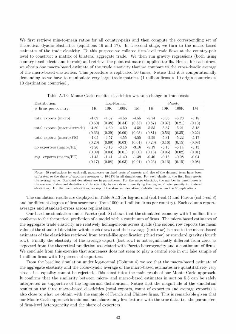
We first retrieve min-to-mean ratios for all country-pairs and then compute the corresponding set oftheoretical dyadic elasticities (equations 16 and 17). In a second stage, we turn to the macro-basedestimates of the trade elasticity. To this purpose we collapse firm-level trade flows at the country-pairlevel to construct a matrix of bilateral aggregate trade. We then run gravity regressions (both usingcountry fixed effects and tetrads) and retrieve the point estimate of applied tariffs. Hence, for each draw,we obtain one macro-based estimate of the trade elasticity that we compare to the cross-dyadic averageof the micro-based elasticities. This procedure is replicated 50 times. Notice that it is computationallydemanding as we have to manipulate very large trade matrices (1 million firms × 10 origin countries ×10 destination countries) .

Table A.13: Monte Carlo results: elasticities wrt to a change in trade costs

Distribution: Log-Normal Pareto

# firms per country: 1K 10K 100K 1M 1K 10K 100K 1M

total exports (micro) -4.69 -4.57 -4.56 -4.55 -5.74 -5.36 -5.23 -5.18(0.60) (0.38) (0.34) (0.33) (0.87) (0.37) (0.21) (0.13)

total exports (macro/tetrads) -4.80 -4.60 -4.59 -4.58 -5.55 -5.37 -5.21 -5.18(0.66) (0.29) (0.09) (0.03) (0.81) (0.56) (0.35) (0.22)

total exports (macro/FE) -4.65 -4.57 -4.55 -4.55 -5.59 -5.31 -5.22 -5.17(0.20) (0.09) (0.03) (0.01) (0.29) (0.16) (0.15) (0.08)

nb exporters (macro/FE) -3.20 -3.16 -3.16 -3.16 -5.19 -5.15 -5.14 -5.13(0.09) (0.03) (0.01) (0.00) (0.13) (0.05) (0.02) (0.01)

avg. exports (macro/FE) -1.45 -1.41 -1.40 -1.39 -0.40 -0.15 -0.08 -0.04(0.17) (0.08) (0.03) (0.01) (0.26) (0.16) (0.15) (0.08)

Notes: 50 replications for each cell, parameters on fixed costs of exports and size of the demand term have beencalibrated so the share of exporters averages to 10-11% in all simulations. For each elasticity, the first line reportsthe average value. Standard deviations are in parentheses. For the micro elasticity, the number in parentheses isthe average of standard deviations of the elasticity in each draw (quantifying the degree of heterogeneity in bilateralelasticities). For the macro elasticities, we report the standard deviation of elasticities across the 50 replications.

The simulation results are displayed in Table A.13 for log-normal (col.1-col.4) and Pareto (col.5-col.8)and for different degrees of firm scarceness (from 1000 to 1 million firms per country). Each column reportsaverages and standard errors across replications.

Our baseline simulation under Pareto (col. 8) shows that the simulated economy with 1 million firmsconforms to the theoretical prediction of a model with a continuum of firms. The micro-based estimates ofthe aggregate trade elasticity are relatively homogeneous across dyads (the second row reports the meanvalue of the standard deviation within each draw) and their average (first row) is close to the macro-basedestimates of the elasticities retrieved from tetrad-like specification (third row) or standard gravity (fourthrow). Finally the elasticity of the average export (last row) is not significantly different from zero, asexpected from the theoretical prediction associated with Pareto heterogeneity and a continuum of firms.We conclude from this exercise that scarceness does not seem to play a central role in our fake sample of1 million firms with 10 percent of exporters.

From the baseline simulation under log-normal (Column 4) we see that the macro-based estimate ofthe aggregate elasticity and the cross-dyadic average of the micro-based estimates are quantitatively veryclose - i.e. equality cannot be rejected. This constitutes the main result of our Monte Carlo approach.It confirms that the similarity between micro- and macro-based estimates in section 5.3 can be safelyinterpreted as supportive of the log-normal distribution. Notice that the magnitude of the simulationresults on the three macro-based elasticities (total exports, count of exporters and average exports) isalso close to what we obtain with the sample of French and Chinese firms. This is remarkable given thatour Monte Carlo approach is minimal and shares only few features with the true data, i.e. the parametersof firm-level heterogeneity and the share of exporters.

43

From Micro to Macro: Demand, Supply, and Heterogeneity … · From Micro to Macro: Demand, Supply,...

Documents

Transcript of From Micro to Macro: Demand, Supply, and Heterogeneity … · From Micro to Macro: Demand, Supply,...