From Micro to Macro: Demand, Supply, and Heterogeneity in ... · and Heterogeneity in the Trade...
52
Highlights We show that heterogeneity in firm performance generates heterogeneous aggregate trade elasticities under distributions other than the Pareto. We estimate firm-level trade elasticity to tariffs, with an average value around -5. Predictions of the model with a log-normal distribution dominate predictions arising with Pareto. From Micro to Macro: Demand, Supply, and Heterogeneity in the Trade Elasticity No 2015-07 – June Working Paper Maria Bas, Thierry Mayer & Mathias Thoenig
Transcript of From Micro to Macro: Demand, Supply, and Heterogeneity in ... · and Heterogeneity in the Trade...

Highlights
We show that heterogeneity in firm performance generates heterogeneous aggregate trade elasticities under distributions other than the Pareto.
We estimate firm-level trade elasticity to tariffs, with an average value around -5.
Predictions of the model with a log-normal distribution dominate predictions arising with Pareto.
From Micro to Macro: Demand, Supply, and Heterogeneity in the Trade Elasticity
No 2015-07 – June Working Paper
Maria Bas, Thierry Mayer & Mathias Thoenig
CEPII Working Paper From Micro to Macro: Demand, Supply, and Heterogeneity in the Trade Elasticity
Abstract Models of heterogeneous firms with selection into export market participation generically exhibit aggregate trade elasticities that vary across country-pairs. Only when heterogeneity is assumed Pareto-distributed do all elasticities collapse into an unique elasticity, estimable with a gravity equation. This paper provides a theory-based method for quantifying country-pair specific elasticities when moving away from Pareto, i.e. when gravity does not hold. Combining two firm-level customs datasets for which we observe French and Chinese individual sales on the same destination market over the 2000-2006 period, we are able to estimate all the components of the dyadic elasticity: i) the demand-side parameter that governs the intensive margin and ii) the supply side parameters that drive the extensive margin. These components are then assembled under theoretical guidance to calculate bilateral aggregate elasticities over the whole set of destinations, and their decomposition into different margins. Our predictions fit well with econometric estimates, supporting our view that micro-data is a key element in the quantification of non-constant macro trade elasticities.
KeywordsTrade elasticity, Firm-level data, Heterogeneity, Gravity, Pareto, Log-normal.
JELF21.
CEPII (Centre d’Etudes Prospectives et d’Informations Internationales) is a French institute dedicated to producing independent, policy-oriented economic research helpful to understand the international economic environment and challenges in the areas of trade policy, competitiveness, macroeconomics, international finance and growth.
CEPII Working PaperContributing to research in international economics
© CEPII, PARIS, 2015
All rights reserved. Opinions expressed in this publication are those of the author(s) alone.
Editorial Director: Sébastien Jean
Production: Laure Boivin
No ISSN: 1293-2574
CEPII113, rue de Grenelle75007 Paris+33 1 53 68 55 00
www.cepii.frPress contact: [email protected]
Working Paper

CEPII Working Paper From Micro to Macro: Demand, Supply, and Heterogeneity in the Trade Elasticity
1. Introduction
The response of trade flows to a change in trade costs, the aggregate trade elasticity, is a centralelement in any evaluation of the welfare impacts of trade liberalization. Arkolakis et al. (2012)recently showed that this parameter, denoted ε for the rest of the paper, is actually one of the(only) two sufficient statistics needed to calculate Gains From Trade (GFT) under a surprisinglylarge set of alternative modeling assumptions—the ones most commonly used by recent researchin the field. Measuring those elasticities has therefore been the topic of a long-standing literaturein international economics.1 The most common usage (and the one recommended by Arkolakiset al., 2012) is to estimate this elasticity in a macro-level bilateral trade equation that Head andMayer (2014) label structural gravity. In order for this estimate of ε to be relevant for a particularexperiment of trade liberalization, it is crucial for this bilateral trade equation to be correctlyspecified as a structural gravity model with, in particular, a unique elasticity to be estimated acrossdyads.
Our starting point is that the model of heterogeneous firms with selection into export marketparticipation (Melitz, 2003) will in general exhibit a dyad-specific elasticity, i.e. an εni , whichapplies to each country pair. Only when heterogeneity is assumed Pareto-distributed do all εnicollapse to a single ε. Under any other distributional assumption, obtaining an estimate of theaggregate trade elasticity from a macro-level bilateral trade equation becomes problematic, sincethere is a now a whole set of εni to be estimated, and structural gravity does not hold anymore.We argue that in this case quantifying trade elasticities at the aggregate level makes it necessary touse micro-level information. To this purpose we exploit a rich panel that combines sales of Frenchand Chinese exporters over 2000-2006 on many destination-product combinations for which wealso observe the applied tariff. We propose a theory-based method using this firm-level exportdata for estimating all the components of the dyad-specific trade elasticity: i) the demand-sideparameter that governs the intensive margin and ii) the supply side parameters that drive theextensive margin. These components are then assembled under theoretical guidance to calculatethe dyadic aggregate elasticities over the whole set of destination-product.
Taking into account cross-dyadic heterogeneity in trade elasticities is crucial for quantifying theexpected impact of various trade policy experiments. Consider the example of the current nego-tiations over a transatlantic trade agreement between the USA and the EU (TTIP). Under thesimplifying assumption of a unique elasticity, whether the trade liberalization takes place with aproximate vs distant, large vs small economy, etc. is irrelevant in terms of trade-promoting ef-fect or welfare gains calculations. By contrast, our results suggest that the relevant εni should besmaller (in absolute value) than if the United States were considering a comparable agreement withcountries where the expected volume of trade is smaller. Regarding welfare, Melitz and Redding(2015) and Head et al. (2014) have shown theoretically that the GFT can be quite substantially
1Recent debates in this literature have concerned the choice of an appropriate source of identification (exchange rateversus tariff changes in particular), aggregation issues (Imbs and Méjean, 2014; Ossa, 2012, for instance), and howthose elasticities might vary according to the theoretical model at hand (Simonovska and Waugh, 2012).
1

CEPII Working Paper From Micro to Macro: Demand, Supply, and Heterogeneity in the Trade Elasticity
mis-estimated if one assumes a constant trade elasticity when the “true” elasticity is variable (themargin of error can exceed 100 percent in both papers). The expected changes in trade patternsand welfare effects of agreements such as TTIP will therefore be different compared to the uniqueelasticity case. One of the main objectives of our paper is to quantify how wrong can one be whenmaking predictions based on a constant trade elasticity assumption.
Our approach maintains the traditional CES (σ) demand system combined with monopolistic com-petition. It features several steps that are structured around the following decomposition of ag-gregate trade elasticity into the sum of the intensive margin and the (weighted) extensive margin:
εni = 1− σ︸ ︷︷ ︸intensive margin
+1
xni/xMINni︸ ︷︷ ︸
min-to-mean
×d lnNnid ln τni︸ ︷︷ ︸
extensive margin
, (1)
The weight is the mean-to-min ratio, our observable measuring the dyadic dispersion of firm-levelperformance, that is defined as the ratio of average to minimum sales across markets. Intuitively,the weight of the extensive margin should be decreasing in easy markets where the increasingpresence of weaker firms augments productivity dispersion. When assuming Pareto with shapeparameter θ, the last part of the elasticity reduces to σ− 1− θ, and the overall elasticity becomesconstant and reflects only the supply side homogeneity in the distribution of productivity: εPni =
εP = −θ (Chaney, 2008).
Our first step aims to estimate the demand side parameter σ using firm-level exports. Sinceprotection is imposed on all firms from a given origin, higher demand and lower protection are notseparately identifiable when using only one country of exports. With CES, firms are all confrontedto the same aggregate demand conditions. Thus, considering a second country of origin enables toisolate the effects of trade policy, if the latter is discriminatory. We therefore combine shipmentsby French and Chinese exporters to destinations that confront those firms with different levels oftariffs. Our setup yields a firm-level gravity equation specified as a ratio-type estimation so asto eliminate unobserved characteristics of both the exporting firm and the importer country, whilekeeping tariffs in the regression. This approach is in many ways akin to using high-dimensional fixedeffects, with the big advantage of easing the computational burden in our context that includesmany firms exporting to numerous destinations. This method is called tetrads by Head et al.(2010) since it combines a set of four trade flows into an ratio of ratios called an export tetradand regresses it on a corresponding tariff tetrad for the same product-country combinations.2 Ouridentification strategy relies on there being enough variation in tariffs applied by different destinationmarkets to French and Chinese exporters. We therefore use in our main specification the last yearbefore the entry of China into WTO in 2001 in cross-section estimations. We also exploit the
2Other work in the literature also relies on the ratio of ratios estimation. Romalis (2007) uses a similar method toestimate the effect of tariffs on trade flows at the product-country level. He estimates the effects of applied tariffchanges within NAFTA countries (Canada and Mexico) on US imports at the product level. Hallak (2006) estimatesa fixed effects gravity model and then uses a ratio of ratios method in a quantification exercise. Caliendo and Parro(2015) also use ratios of ratios and rely on asymmetries in tariffs to identify industry-level elasticities.
2

CEPII Working Paper From Micro to Macro: Demand, Supply, and Heterogeneity in the Trade Elasticity
panel dimension of the data over the 2000-2006 period. We explore different sources of variance inthe data with comparable estimates of the intensive margin trade elasticity that imply an averagevalue of σ around 5.
Our second step applies equation (1) and assembles the estimates of the intensive margin (σ)with the central supply side parameter —reflecting dispersion in the distribution of productivity—estimated on the same datasets, to obtain predicted aggregate elasticities of total export, number ofexporters and average exports to each destination. Those dyadic predictions (one elasticity for eachexporter-importer combination) require knowledge of the bilateral export productivity cutoff underwhich firms find exports to be unprofitable. We also make use of the mean-to-min ratio to revealthose cutoffs. A key element of our procedure is the calibration of the productivity distribution.As an alternative to Pareto we consider the log-normal distribution that fits the micro-data onfirm-level sales very well. We show that under log-normal the εni are larger (in absolute value) forpairs with low volumes of trade. Hence the trade-promoting impact of liberalization is expected tobe larger for this kind of trade partners. A side result of our paper is to discriminate between Paretoand log-normal as potential distributions for the underlying firm-level heterogeneity, suggesting thatlog-normal does a better job at matching the non-unique response of exports to changes in tradecosts. Two pieces of evidence in that direction are provided.3 The first provides direct evidencethat aggregate elasticities are non-constant across dyads. The second is a positive and statisticallysignificant correlation across industries between firm-level and aggregate elasticities–at odds withthe prediction of a null correlation under Pareto. We also find that the heterogeneity in tradeelasticities is quantitatively important: Although the cross-dyadic average of bilateral elasticities isquite well approximated by a standard gravity model constraining the estimated parameter to beconstant, deviations from this average level can be large. For Chinese exports, assuming a uniqueelasticity would yield to underestimate the trade impact of a tariff liberalization by about 25%for countries with initially very small trade flows (Somalia, Chad or Azerbaijan for instance). Bycontrast, the error would be to overestimate by around 12.5 percent the exports created when theUnited States or Japan reduce their trade costs.
Our paper clearly fits into the empirical literature estimating trade elasticities. Different approachesand proxies for trade costs have been used, with an almost exclusive focus on aggregate countryor industry-level data. The gravity approach to estimating those elasticities mostly uses tariff datato estimate bilateral responses to variation in applied tariff levels. Most of the time, identificationis in the cross-section of country pairs, with origin and destination determinants being controlledthrough fixed effects (Baier and Bergstrand (2001), Head and Ries (2001), Caliendo and Parro(2015), Hummels (1999), Romalis (2007) are examples). A related approach is to use the factthat most foundations of gravity have the same coefficient on trade costs and domestic cost
3Head et al. (2014) provide evidence and references for several micro-level datasets that individual sales are muchbetter approximated by a log-normal distribution when the entire distribution is considered (without left-tail truncation).Freund and Pierola (2015) is a recent example showing very large deviations from the Pareto distribution if the datais not vastly truncated for all of the 32 countries used. Our findings complement those papers by providing industry-and aggregate-level evidence on trade elasticities.
3

CEPII Working Paper From Micro to Macro: Demand, Supply, and Heterogeneity in the Trade Elasticity
shifters to estimate that elasticity from the effect on bilateral trade of exporter-specific changes inproductivity, export prices or exchange rates (Costinot et al. (2012) is a recent example).4 Baierand Bergstrand (2001) find a demand side elasticity ranging from -4 to -2 using aggregate bilateraltrade flows from 1958 to 1988. Using product-level information on trade flows and tariffs, thiselasticity is estimated by Head and Ries (2001), Romalis (2007) and Caliendo and Parro (2015)with benchmark average elasticities of -6.88, -8.5 and -4.45 respectively. Costinot et al. (2012)also use industry-level data for OECD countries, and obtains a preferred elasticity of -6.53 usingproductivity based on producer prices of the exporter as the identifying variable. Our paper also hasconsequences for how to interpret those numbers in terms of underlying structural parameters. Witha homogeneous firms model of the Krugman (1980) type in mind, the estimated elasticity turnsout to reveal a demand-side parameter only (this is also the case with Armington differentiationand perfect competition as in Anderson and van Wincoop (2003)). When instead consideringheterogeneous firms à la Melitz (2003), the literature has proposed that the macro-level tradeelasticity is driven solely by a supply-side parameter describing the dispersion of the underlyingheterogeneity distribution of firms. This result has been shown with several demand systems (CESby Chaney (2008), linear by Melitz and Ottaviano (2008), translog by Arkolakis et al. (2010) forinstance), but again relies critically on the assumption of a Pareto distribution. The trade elasticitythen provides an estimate of the dispersion parameter of the Pareto.5 We show here that bothexisting interpretations of the estimated elasticities are too extreme: When the Pareto assumptionis relaxed, the aggregate trade elasticity is a mix of demand and supply parameters.
There is a small set of papers–the most related to the first part of ours–that estimate the intensivemargin elasticity at the firm-level. Berman et al. (2012) presents estimates of the trade elasticitywith respect to real exchange rate variations across countries and over time using firm-level datafrom France. Fitzgerald and Haller (2014) use firm-level data from Ireland, real exchange rateand weighted average firm-level applied tariffs as price shifters to estimate the trade elasticityto trade costs. The results for the impact of real exchange rate on firms’ export sales are ofa similar magnitude, around 0.8 to 1. Applied tariffs vary at the product-destination-year level.Fitzgerald and Haller (2014) create a firm-level destination tariff as the weighted average over allhs6 products exported by a firm to a destination in a year using export sales as weights. Relyingon this construction, they find a tariff elasticity of around -2.5 at the micro level. This is also thepreferred estimates of Berthou and Fontagné (2015), who use the response of the largest Frenchexporters in the United States to the levels of applied tariffs. We depart from those papers by
4Other methodologies (also used for aggregate elasticities) use identification via heteroskedasticity in bilateral flows,and have been developed by Feenstra (1994) and applied widely by Broda and Weinstein (2006) and Imbs and Méjean(2014). Yet another alternative is to proxy trade costs using retail price gaps and their impact on trade volumes, asproposed by Eaton and Kortum (2002) and extended by Simonovska and Waugh (2011).5This result of a constant trade elasticity reflecting the Pareto shape holds when maintaining the CES demand systembut making other improvements to the model such as heterogeneous marketing and/or fixed export costs (Arkolakis,2010; Eaton et al., 2011). In the Ricardian setup of Eaton and Kortum (2002) , the trade elasticity is also a (constant)supply side parameter reflecting heterogeneity, but this heterogeneity takes place at the national level, and reflects thescope for comparative advantage.
4

CEPII Working Paper From Micro to Macro: Demand, Supply, and Heterogeneity in the Trade Elasticity
using an alternative methodology to identify the trade elasticity with respect to applied tariffs; i.e.the differential treatment of exporters from two distinct countries (France and China) in a set ofproduct-destination markets.
Our paper also contributes to the literature studying the importance of the distribution assumptionof heterogeneity for trade patterns, trade elasticities and welfare. Head et al. (2014), Yang (2014),Melitz and Redding (2015) and Feenstra (2013) have recently argued that the simple gains fromtrade formula proposed by Arkolakis et al. (2012) relies crucially on the Pareto assumption, whichmutes important channels of gains in the heterogenous firms case. Barba Navaretti et al. (2015)present gravity-based evidence that the exporting country fixed effects depends on characteristicsof firms’ distribution that go beyond the simple mean productivity, a feature incompatible with theusually specified Pareto heterogeneity. The alternatives to Pareto considered to date in welfaregains quantification exercises are i) the truncated Pareto by Helpman et al. (2008), Melitz andRedding (2015) and Feenstra (2013), and ii) the log-normal by Head et al. (2014) and Yang(2014). A key simplifying feature of Pareto is to yield a constant trade elasticity, which is not thecase for alternative distributions. Helpman et al. (2008) and Novy (2013) have produced gravity-based evidence showing substantial variation in the trade cost elasticity across country pairs. Ourcontribution to that literature is to use the estimated demand and supply-side parameters toconstruct predicted bilateral elasticities for aggregate flows under the log-normal assumption, andcompare their first moments to gravity-based estimates. It is possible to generate bilateral tradeelasticities changing another feature of the standard model. The most obvious is to depart from thesimple CES demand system. Novy (2013) builds on Feenstra (2003), using the translog demandsystem with homogeneous firms to obtain variable trade elasticities. Atkeson and Burstein (2008)is another example maintaining CES demand, and generating heterogeneity in elasticities troughmonopolistic competition. We choose here to keep the change with respect to the benchmarkMelitz/Chaney framework to a minimal extent, keeping CES and monopolistic competition, whilechanging only the distributional assumption.
The next section of the paper describes our model and empirical strategy. The third sectionpresents the different firm-level data and the product-country level tariff data used in the empiricalanalysis. The fourth section reports the estimates of the intensive margin elasticity. Section5 computes predicted macro-level trade elasticities and compares them with estimates from theChinese and French aggregate export data. It also provides two additional pieces of evidence infavor of non-constant trade elasticities. The final section concludes.
2. Empirical strategy for estimating the demand side parameter
2.1. A firm-level export equation
Consider a set of potential exporting firms, all located in the same origin country i and producingproduct p (omitting those indexes for the start of exposition). We use the Melitz (2003)/Chaney(2008) theoretical framework of heterogeneous firms facing constant price elasticity demand (CES
5

CEPII Working Paper From Micro to Macro: Demand, Supply, and Heterogeneity in the Trade Elasticity
utility combined with iceberg costs) and contemplating exports to several destinations. In thissetup, firm-level exports to country n depend upon the firm-specific unit input requirement (α),wages (w), and “real” expenditure in n, XnP σ−1n , with Pn the ideal CES price index relevant forsales in n. There are trade costs associated with reaching market n, consisting of an observableiceberg-type part (τn), and a shock that affects firms differently on each market, bn(α):6
xn(α) =
(σ
σ − 1
)1−σ[αwτnbn(α)]1−σ
XnP 1−σn
(2)
Taking logs of equation (2), and noting with εn(α) ≡ b1−σn our unobservable firm-destination errorterm, and with An ≡ XnP
σ−1n the “attractiveness” of country n (expenditure discounted by the
degree of competition on this market), a firm-level gravity equation can be derived:
ln xn(α) = (1− σ) ln
(σ
σ − 1
)+ (1− σ) ln(αw) + (1− σ) ln τn + lnAn + ln εn(α) (3)
Our objective is to estimate the trade elasticity, 1 − σ identified on cross-country differences inapplied tariffs (that are part of τn). This involves controlling for a number of other determinants(“nuisance” terms) in equation (3). First, it is problematic to proxy for An, since it includes the idealCES price index Pn, which is a complex non-linear construction that itself requires knowledge of σ. Awell-known solution used in the gravity literature is to capture (An) with destination country fixedeffects (which also solves any issue arising from omitted unobservable n-specific determinants).This is however not applicable here since An and τn vary across the same dimension. To separatethose two determinants, we use a second set of exporters, based in a country that faces differentlevels of applied tariffs, such that we recover a bilateral dimension on τ . The firm-level salesbecome
ln xni(α) = (1− σ) ln
(σ
σ − 1
)+ (1− σ) ln(αwi) + (1− σ) ln τni + lnAn + ln εni(α), (4)
where each firm can now be based in one of the two origin countries for which we have customsdata, France and China, i = [FR,CN]. A second issue is that we need to control for firm-levelmarginal costs (αwi). Again measures of firm-level productivity and wages are hard to obtain fortwo different source countries on an exhaustive basis. In addition, there might be a myriad of otherfirm-level determinants of export performance, such as quality of products exported, managerialcapabilities... which will remain unobservable. Capturing those determinants through fixed effectsis an option which proves computationally intensive in our case, since we have a very large panelof exporters that export many products to a large number of countries. We adopt an alternativeapproach, a ratio-type estimation inspired by Hallak (2006), Romalis (2007), Head et al. (2010),and Caliendo and Parro (2015) that removes observable and unobservable determinants for both
6An example of such unobservable term would be the presence of workers from country n in firm α, that wouldincrease the internal knowledge on how to reach consumers in n, and therefore reduce trade costs for that specificcompany in that particular market (b being a mnemonic for barrier to trade). Note that this type of random shock isisomorphic to assuming a firm-destination demand shock in this CES-monopolistic competition model.
6

CEPII Working Paper From Micro to Macro: Demand, Supply, and Heterogeneity in the Trade Elasticity
firm-level and destination factors. This method uses four individual export flows to calculate ratiosof ratios: an approach referred to as tetrads from now on. We now turn to a presentation of thismethod.
2.2. Microfoundations of a ratio-type estimation
To implement tetrads at the micro level, we need firm-level datasets for two origin countriesreporting exports by firm, product and destination country. We also require information on bilateraltrade costs faced by firms when selling their products abroad that differ across exporting countries.We combine French and Chinese firm-level datasets from the corresponding customs administrationwhich report export value by firm at the hs6 level for all destinations in 2000. The firm-level customsdatasets are matched with data on tariffs effectively applied to each exporting country (China andFrance) at the same level of product disaggregation for each destination. Focusing on 2000 allowsus to exploit variation in tariffs applied to each exporter country (France/China) at the productlevel by the importer countries since it precedes the entry of China into WTO at the end of 2001.We also exploit the variation over time of tariffs applied to France and China within products anddestinations, from 2000 to 2006 in a set of robustness checks.
Estimating micro-level tetrads implies dividing product-level exports of a firm located in France tocountry n by the exports of the same product by that same firm to a reference country, denotedk . Then, calculate a similar ratio for a Chinese exporter (same product and countries). Finally theratio of those two ratios uses the multiplicative nature of the CES demand system to get rid of allthe “nuisance” terms mentioned above. Because there is quite a large number of exporters, takingall possible firm-destination-product combinations is not feasible. We therefore concentrate ouridentification on the largest exporters for each product.7 We rank firms based on export value foreach hs6 product and reference importer country (Australia, Canada, Germany, Italy, Japan, NewZealand, Poland and the UK).8 For a given product, taking the ratio of exports of a French firmwith rank j exporting to country n, over the flow to the reference importer country k , removes theneed to proxy for firm-level characteristics in equation (4):
xn(αj,FR)
xk(αj,FR)
=
(τnFR
τkFR
)1−σ×AnAk×εn(α
j,FR)
εk(αj,FR)
(5)
To eliminate the aggregate attributes of importing countries n and k , we need the two sourcesof firm-level exports to have information on sales by destination country. This allows to take theratio of equation (5) over the same ratio for a firm with rank j located in China:
xn(αj,FR)/xk(α
j,FR)
xn(αj,CN)/xk(α
j,CN)=
(τnFR/τkFR
τnCN/τkCN
)1−σ×εn(α
j,FR)/εk(αj,FR)
εn(αj,CN)/εk(α
j,CN). (6)
7Section A.8.3. presents an alternative strategy that keeps all exporters and explicitly takes into account selectionissues.8Those are among the main trading partners of France and China, and also have the key advantage for us of applyingdifferent tariff rates to French and Chinese exporters in 2000.
7

CEPII Working Paper From Micro to Macro: Demand, Supply, and Heterogeneity in the Trade Elasticity
Denoting tetradic terms with a ˜ symbol, one can re-write equation (6) as
x{j,n,k} = τ1−σ{n,k} × ε{j,n,k}, (7)
which will be our main foundation for estimation.
2.3. Estimating equation
With equation (7), we can use tariffs to identify the firm-level trade elasticity, 1 − σ. Restoringthe product subscript (p), and using i = FR or CN as the origin country index, we specify bilateraltrade costs as a function of applied tariffs, with ad valorem rate tpni and of a collection of otherbarriers, denoted with Dni . Those include the classical gravity covariates such as distance, commonlanguage, colonial link and common border. Taking the example of a continuous variable such asdistance for Dni :
τpni = (1 + tpni)Dδni , (8)
which, once introduced in the logged version of (7) leads to our estimable equation
ln xp{j,n,k} = (1− σ) ln˜(
1 + tp{n,k}
)+ (1− σ)δ ln D{n,k} + ln εp{j,n,k}. (9)
The dependent variable corresponds to the ratio of ratios of exports for a certain rank j . In order toobtain a valid observation for each product, we iterate from j = 1 to 10, that is firms ranking fromthe top to the 10th exporter for a given product. Our precise procedure is the following: Firms areranked according to their export value for each product and reference importer country k . We thentake the tetrad of exports of the top French firm over the top Chinese firm exporting the sameproduct to the same destination. The set of destinations for each product is therefore limited tothe countries where both the top French and Chinese firm export that product, in addition to thereference country. In order to have enough variation in the dependent variable, we fill in the missingexport values of each product-destination-reference with lower ranked export tetrads (until rank10): For each product×destination×reference, we start with the top Chinese exporter (j = 1) flowwhich divides French exporter’s flow iterating the French firm over j = 2 to 10, until a non-missingtetrad is generated. If the tetrad is still missing, the procedure then goes to the Chinese exporterranked j = 2 and restarts iterating until Chinese exporter ranked j = 10 is reached.
It is apparent in equation (9) that the identification of the effect of tariffs is possible over several di-mensions: essentially across i) destination countries and ii) products, both interacted with varianceacross reference countries. In our baseline cross-section estimations, we investigate the variousdimensions, by sequentially including product-reference or destination-reference fixed effects to thebaseline specification. In the panel estimations reported as robustness checks in the appendix, weexploit variation of tariffs within products-destinations over time and across reference countrieswith product-destination, year and importing reference country fixed effects. There might be un-observable destination country characteristics, such as political factors or uncertainty on tradingconditions, that can generate a correlated error-term structure, potentially biasing downwards the
8

CEPII Working Paper From Micro to Macro: Demand, Supply, and Heterogeneity in the Trade Elasticity
standard error of our variable of interest. Hence, standard errors are clustered at the destinationlevel in the baseline specifications.9
Finally, one might be worried by the presence of unobserved bilateral trade costs that might becorrelated with our measure of applied tariffs. Even though it is not clear that the correlation withthose omitted trade costs should be systematically positive, we use, as a robustness check, a moreinclusive measure of applied trade costs, the Ad Valorem Equivalent (AVE) tariffs from WITS andMAcMAp databases, described in the next section.
3. Data
• Trade: Our dataset combines Chinese and French firm-level exports for the year 2000. TheFrench trade data comes from the French Customs, which provide annual export data at theproduct level for French firms.10 The customs data are available at the 8-digit product levelCombined Nomenclature (CN) and specify the country of destination of exports. The free onboard (f.o.b) value of exports is reported in euros and we converted those to US dollars usingthe real exchange rate from Penn World Tables for 2000. The Chinese transaction data comesfrom the Chinese Customs Trade Statistics (CCTS) database which is compiled by the GeneralAdministration of Customs of China. This database includes monthly firm-level exports at the8-digit HS product-level (also reported f.o.b) in US dollars. The data is collapsed to yearlyfrequency. The database also records the country of destination of exports. In both cases,export values are aggregated at the firm-product(hs6)-destination level in order to match withapplied tariffs information that are available at the hs6-destination level.11
• Tariffs: Tariffs come from the WITS (World Bank) database.12 We rely on the ad valoremrate effectively applied at the hs6 level by each importer country to France and China. In ourcross-section analysis performed for the year 2000 before the entry of China into the WorldTrade Organization (WTO), we exploit different sources of variation within hs6 products acrossimporting countries on the tariff applied to France and China. The first variation naturallycomes from the European Union (EU) importing countries that apply zero tariffs to trade withEU partners (like France) and a common external tariff to extra-EU countries (like China). Thesecond source of variation in the year 2000 is that several non-EU countries applied the Most
9Since the level of clustering (destination country) is not nested within the level of fixed effects and the number ofclusters is quite small with respect to the size of each cluster, we also implement the solution proposed by Wooldridge(2006). He recommends to run country-specific random effects on pair of firms demeaned data, with a robustcovariance matrix estimation. This methodology is also used by Harrigan and Deng (2010) who encounter a similarproblem. The results, available upon request, are robust under this specification.10This database is quite exhaustive. Although reporting of firms by trade values below 250,000 euros (within the EU)or 1,000 euros (rest of the world) is not mandatory, there are in practice many observations below these thresholds.11The hs6 classification changes over time. During our period of analysis it has only changed once in 2002. To takeinto account this change in the classification of products, we have converted the HS-2002 into HS-1996 classificationusing WITS conversion tables.12Information on tariffs is available at http://wits.worldbank.org/wits/
9

CEPII Working Paper From Micro to Macro: Demand, Supply, and Heterogeneity in the Trade Elasticity
Favored Nation tariff (MFN) to France, while the effective tariff applied to Chinese productswas different (since China was not yet a member of WTO). We describe those countries andtariff levels below.
• Gravity controls: In all estimations, we include additional trade barriers variables that determinebilateral trade costs, such as distance, common (official) language, colony and common border(contiguity). The data come from the CEPII distance database.13 We use the population-weighted great circle distance between the set of largest cities in the two countries.
3.1. Reference importer countries
The use of a reference country, k in equation (5), is crucial for a consistent identification of thetrade elasticity. We choose reference importer countries with two criteria in mind. First, thesecountries should be those that are the main trade partners of France and China in the year 2000,since we want to minimize the number of zero trade flows in the denominator of the tetrad. Thesecond criteria relies on the variation in the tariffs effectively applied by the importing country toFrance and China. Hence, among the main trade partners, we retain those countries for whichthe average difference between the effectively applied ad valorem tariffs to France and China isgreater. These two criteria lead us to select the following set of 8 reference countries: Australia,Canada, Germany, Italy, Japan, New Zealand, Poland and the UK. Tables A.3 and A.4 in theappendix present, for each destination country, the count of products for which the difference intariffs applied to France and China is positive, negative or zero, together with the average tariffgap.
For the sake of exposition, our descriptive analysis of reference countries relates only to the twomain relevant trade partners of France and China in our sample. In the case of France, the maintrade partner is Germany. The main trade partner of China is the US and the second one is Japan.Given that the US has applied the MFN tariff to China in several products before the entry of Chinain WTO, there is almost no variation in the difference in effectively applied ad valorem tariffs bythe US to France and China in 2000. Hence, we use in the following descriptive statistics Germanyand Japan as reference importer countries.
The difference in the effectively applied tariffs to France and China at the industry level by referenceimporter country (Germany and Japan) is presented in figure 1 (with precise numbers provided inthe appendix, Table A.1). As can be noticed, there is a significant variation across 2-digit industriesin the average percentage point difference in applied tariffs to both exporting countries in the year2000. This variation is even more pronounced at the hs6 product level. Our empirical strategy willexploit this variation within hs6 products and across destination countries.
13This dataset is available at http://www.cepii.fr/anglaisgraph/bdd/distances.htm
10

CEPII Working Paper From Micro to Macro: Demand, Supply, and Heterogeneity in the Trade Elasticity
Figure 1 – Average percentage point difference between the applied tariff to France and Chinaacross industries by Germany and Japan (2000)
-10 -5 0 5 10
Importer: JPN
Importer: DEU
LeatherWearing apparel
TextileWood
ChemicalRubber & Plastic
FurnitureBasic metal products
PaperMetal products
FoodNon Metallic
Coke prodElectrical Prod
EditionMachinery
Medical instrumentsAgricultureTransportVehicles
Equip. Radio, TVOffice
Coke prodPaperOffice
MachineryElectrical Prod
FurnitureMedical instruments
Metal productsEdition
ChemicalTransport
WoodRubber & Plastic
Non MetallicLeather
Equip. Radio, TVBasic metal products
VehiclesAgriculture
TextileFood
Wearing apparel Full sampleTetradregression sample
Source: Authors’ calculation based on Tariff data from WITS (World Bank).

CEPII Working Paper From Micro to Macro: Demand, Supply, and Heterogeneity in the Trade Elasticity
3.2. Estimating sample
Our dependent variable is the log of a ratio of ratios of firm-level exports of firms with rank j ofproduct p to destination n. The two ratios use the French/Chinese origin of the firm, and thereference country dimension k .
Firms are ranked according to their export value for each hs6 line and reference importer country.We first take the ratio of ratios of exports of the top 1 French and Chinese firms and then wecomplete the missing export values for hs6 product-destination pairs with lower ranked firms (top2 to top 10). The final estimating sample is composed of 99,645 (37,396 for the top 1 exportingfirm) product-destination-reference country observations in the year 2000.
The number of hs6 products and destination countries used in estimation is lower than the onesavailable in the original French and Chinese customs datasets since we need that the top 1 (to top10) French exporting firm exports the same hs6 product that the top 1 (to top 10) Chinese exportingfirm to at least the reference country as well as the destination country. The total number of hs6products in the estimating sample is 2649. The same restriction applies to destination countries.We manage to keep 74 such destination countries.
Table A.2 in the appendix presents descriptive statistics of the main variables at the destinationcountry level for the countries present in the estimating sample. It reports population and GDPfor each destination country in 2000, as well as the ratios of total exports, average exports, totalnumber of exporting firms, and distance between France and China. Only 12 countries in ourestimating sample are closer to China than to France. In all of those, the number of Chineseexporters is larger than the number of French exporters, and the total value of Chinese exportslargely exceeds the French one. On the other end of the spectrum, countries like Belgium andSwitzerland witness much larger counts of exporters and total flows from France than from China,as expected.
4. Estimates of the demand side parameter
4.1. Graphical illustration
Before estimation, we turn to describing graphically the relationship between export flows and ap-plied tariffs tetrads for different destination countries across products. In the interest of parsimonywe focus again on the two main reference importer countries (k is Germany or Japan) and a re-stricted set of six destination countries (n is Australia, Brazil, USA, Canada, Poland or Thailand).We calculate for each hs6 product p the tetradic terms for exports of French and Chinese firmsranked j = 1 to 10th as ln xp{j,n,k} = ln xpn (αj,FR)− ln xpk (αj,FR)− ln xpn (αj,CN) + ln xpk (αj,CN) and the
tetradic term for applied tariffs at the same level as ln ˜(1 + tp{n,k}) = ln(1 + tpnFR)− ln(1 + tpkFR)−ln(1 + tpnCN) + ln(1 + tpkCN),
12

CEPII Working Paper From Micro to Macro: Demand, Supply, and Heterogeneity in the Trade Elasticity
Figure 2 report these tetrad terms to document the raw (and unconditional) evidence of the effectof tariffs on exported values by individual firms. The graphs also display the regression line andestimated coefficients of this simple regression of the logged export tetrad on the log of tarifftetrad for each of the six destination countries. Each point corresponds to a given hs6 product,and we highlight the cases where the export tetrad is calculated out of the largest (j = 1) Frenchand Chinese exporters with a circle. The observations corresponding to Germany as a referenceimporter country are marked by a triangle, when the symbol is a square for Japan.
These estimations exploit the variation across products on tariffs applied by the destination countryn and reference importer country k to China and France. In all cases, the estimated coefficienton tariff is negative and highly significant as shown by the slope of the line reported in each ofeach graphs. Those coefficients are quite large in absolute value, denoting a very steep responseof consumers to differences in applied tariffs.
Figure 3 exposes a different dimension of identification, by looking at the impact of tariffs forspecific products. We graph, following the logic of Figure 2 the tetrad of export value againstthe tetrad of tariffs for six individual products, which are the ones for which we maximize thenumber of observations in the dataset. Again (apart from the tools sector, where the relationshipis not significant), all those sectors exhibit strong reaction to tariff differences across importingcountries. A synthesis of this evidence for individual sectors can be found by averaging tetradsover a larger set of products. We do that in Figure 4 for the 184 products that have at least 30destinations in common in our sample for French and Chinese exporters. The coefficient is againvery large in absolute value and highly significant. The next section presents regression resultswith the full sample, both dimensions of identification, and the appropriate set of gravity controlvariables which will confirm this descriptive evidence and, as expected reduce the steepness of theestimated response.
4.2. The intensive margin
This section presents the estimates of the trade elasticity with respect to applied tariffs fromequation (9) for all reference importer countries (Australia, Canada, Germany, Italy, Japan, NewZealand, Poland and the UK) pooled in the same specification. In all specifications standard errorsare clustered by destination×reference country.
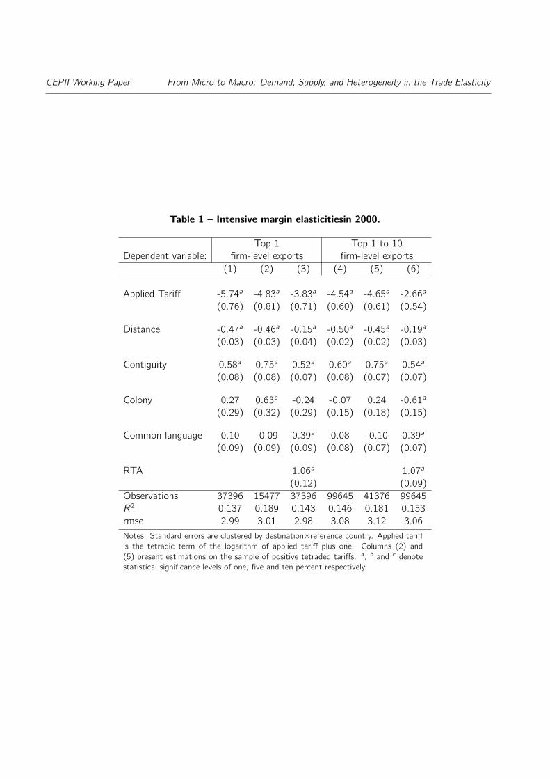
Estimations in Table 1 exploit the variations in tariffs applied to France and China across bothproducts and destination countries. Columns (1) to (3) show the results using as dependent variablethe ratio of the top 1 exporting French and Chinese firm. Columns (2) presents estimations on thesample of positive tetraded tariffs and column (3) controls for the tetradic terms of Regional TradeAgreements (RTA). Columns (4) to (6) of Table 1 present the estimations using as dependentvariable the ratio of firm-level exports of the top 1 to the top 10 French and Chinese firms. Theseestimations yield coefficients for the applied tariffs (1 − σ) that range between -5.74 and -2.66.Note that in both cases, the coefficients on applied tariffs are reduced when including the RTA,
13

CEPII Working Paper From Micro to Macro: Demand, Supply, and Heterogeneity in the Trade Elasticity
Figure 2 – Unconditional tetrad evidence: by importer
.01
110
010
000
Expo
rt te
trad
.9 1 1.1 1.2Tariff tetrad
Ref. country: JPNRef. country: DEURank 1 tetrad
Note: The coefficient on tariff tetrad is -18.99 with a standard error of 3.34
Destination country: AUS
.01
110
010
000
Expo
rt te
trad
.9 .95 1 1.05 1.1Tariff tetrad
Ref. country: JPNRef. country: DEURank 1 tetrad
Note: The coefficient on tariff tetrad is -31.11 with a standard error of 5.83
Destination country: BRA
.01
110
010
000
Expo
rt te
trad
.9 1 1.1 1.2Tariff tetrad
Ref. country: JPNRef. country: DEURank 1 tetrad
Note: The coefficient on tariff tetrad is -20.11 with a standard error of 2.21
Destination country: USA
.01
110
010
000
Expo
rt te
trad
.9 1 1.1 1.2 1.3Tariff tetrad
Ref. country: JPNRef. country: DEURank 1 tetrad
Note: The coefficient on tariff tetrad is -14.19 with a standard error of 2.79
Destination country: CAN
.01
110
010
000
Expo
rt te
trad
.8 1 1.2 1.4 1.6Tariff tetrad
Ref. country: JPNRef. country: DEURank 1 tetrad
Note: The coefficient on tariff tetrad is -12.92 with a standard error of 2.55
Destination country: POL
.01
110
010
000
Expo
rt te
trad
.9 1 1.1 1.2 1.3Tariff tetrad
Ref. country: JPNRef. country: DEURank 1 tetrad
Note: The coefficient on tariff tetrad is -23.87 with a standard error of 4.91
Destination country: THA

CEPII Working Paper From Micro to Macro: Demand, Supply, and Heterogeneity in the Trade Elasticity
Figure 3 – Unconditional tetrad evidence: by product
NZL
FIN
NLD
POL
IRL
PRTGRC
NOR
AUT
GBR
JPN
DEUSWEESPDNK
BEL
ITA
DEU
ESPPOL
GRC
SWE
IRL
NLD
ITA
FIN
AUT
NZL
DNK
GBRNOR
BEL
JPN
MLT
BRA
CHL
CAN
MAR
TWN
POLVEN
NOR
AUS JPN
NZL
IDN
THA
BGRMEX
CHECZE
SAUARG
LBN
USA
CYP
MEXLBN
THAJPN
CAN
TWNBGR
NOR
AUS
ARG
MLTVEN
CZE
NZL
CYPMARSAU
POLBRACHL
USA
CHE
IDN
LBN
USA
CHE
SAU
MLT
EST
NOR CYP
MAR
IDNARG
TWN
NZL
JPN
THA
CANAUS
POL
BRA
CZE
MEX
DEU
THA
POL
VEN
URY
LBN
CZE
MEX
ARGIDN
IRL
NZL
NLDFIN
GBR
MAR
AUT
TWN
DNK
CHL
GRC
CYP
SAU
NOR MLT
CHE
CAN
BEL
ITA
BRA
USA
PRTSWEESP
AUS
DEUDNKITA
ARG
TWN
GRC
JPN
CYPAUT
FIN
SAU
CZE
VEN
MAR
POL
NLD
THA
IRL
CAN
AUS
BEL MLT
CHL
CHE
USAIDN
NOR
GBR
MEXLBN
BRA
SWE
CAN
ITA
CYPLBN
USA
THA
JOR
AUT
IRLNLD
NZL
JPN
SAU
BEL CHE
CHL
GRC
VENDEU
IDN
MEX
BGR
BRA
PRTESTCZE
DNKARG
FIN
NOR
ESPSWE
MLT
AUS
MAR
GBR
TWN
.01
.11
1010
010
000
Expo
rt te
trad
.95 1 1.05Tariff tetrad
Ref. countries: AUSCANJPNNZLPOLDEUGBRITA
Note: The coefficient on tariff tetrad is -24.25 with a standard error of 3.5.
HS6 product: Toys nes
SWE
POL
BEL
DNKPRT
DEU
CAN
FIN
NLD
NOR
IRLJPN
GRC
GBR
ITA
ESP
CHE
USABRA
ESP
GBR
GRC
NLD
JPN
CZE
POL
MARDEU
PRT
CHLBEL
FIN
DNK AUS
AUT
VEN
SWEDOMCYPGTM
PHL
NOR
NZL
SAU
SAU
MAR
JPN
CYP
USAVEN
CZE
POL
NOR
AUS
CRI
JOR
CAN
CHEBRN
BRA
CHL
NZL
EST
SLV
TWN
THA
GTM
ARG
NOR
CAN
AUSURYCHL
LBN
EST
YEM
USA
JPN
POL
BRN
THA
CYP
PAN
BRA
CHE
GTM
SLV
COL
DOM
MLT
VEN
SAUGAB
CHL
JORURY
DOM
TWNTHA
AUS
CHE
NZL
MARGTMARGJAM
BRB
PAN
VEN
LBN
YEM
MLT
GBR
SWEESP
THA
MEX
VEN
BRN
AUT
GTM
FIN
POL
GRC BRA
CAN
DNK
CHE
AUSTWN
USA
CHLNOR
DEU
DEUSWEDNK
GRC
ESP
PRTNORBEL
CAN
ITA
NLD
POL
FIN
AUT JPN
CYP
GRC
GTM
NOR
FIN
CHE
CZE
DEUIRL
BRAESP
TWN
AUS
GBR
SAU
NZLJOR
DNK
SWE
CHL
BEL
CANUSA
NLDAUT
.01
.11
1010
010
000
Expo
rt te
trad
.95 1 1.05Tariff tetrad
Ref. countries: AUSCANJPNNZLPOLDEUGBRITA
Note: The coefficient on tariff tetrad is -8.83 with a standard error of 2.61.
HS6 product: Tableware and kitchenware
ITA
PRT
FIN
BEL NZL
ESPSWE
NLD
DNK
GRC
CANGBR
DEUPOL
AUTSAU
AUS
PRY
AUT
NLD
VEN
DNK
LBN
FINBEL
USA
GBR
NZL
ESPGRC
CHLNGA
ITA
SWE
POL
PRT
IRN
BRAPERDEU
ARG
THA
IDN
JOR
TWN
PHL
GHA
URY
CYP
CHE
JPN
MEX
LKA
BRA
POL
VEN
LKACZE
PAN
CYP
JOR
URY
GHA
JPN
TWN
MEX
CHL
IRN
PER
USA
LBNNZL
THA
CHE
SAU
ARGNGAPHL
CANPRYAUS
IDN
TWN
PRY
BRAMEXNZL
AUS
GHA
CANLKA
SAU
CHEJOR
CHLTHAPANUSA
VEN
JPNARGPER
CYPIRN
PHL
URY
MLT
PER
ARG
AUSURY
CHL
USAPHL
CHE
PAN
CZE
IRN
VEN
CAN
JPNTHA
NGABRASAU
GHA
NZL
MEXJORCYP
POL
IDN
TWN
PRY
LBN
LKA
ESP
DNKCAN
ITAAUT
BEL
FIN
POLNLD
NZL
GBRDEUSWEGRC
PRTCHE
POL
NLD
URY
THA
USA
FIN
LKA
BEL
PERGHA
AUSCYP
SAU
AUTLBN
CAN
IDN
GBR
PHL
ITA
MEX
SWE
CHL
ARG
VEN
PRY
ESP
NGA
PRT
GRCDEU
TWN
JORDNK
JPN
IRN
BRA
IDN
SAU
CHE
VEN
BEL
PRYAUTLKA
TWN
PER
GBR
DEU
JOR
SWE
JPN
NZL CAN
PHL
GRC
PRT
ITA
ESP
ARG
GHA
USA
BRA
CYP
LBNNGA
CZE
CHL
THA
NLD
IRN
PAN
URYAUS
MEX
DNK
.01
.11
1010
010
000
Expo
rt te
trad
.95 1 1.05Tariff tetrad
Ref. countries: AUSCANJPNNZLPOLDEUGBRITA
Note: The coefficient on tariff tetrad is -9.54 with a standard error of 3.12.
HS6 product: Domestic food grinders
ESPDNK
POL
NOR GBR
DEU
GRCNLD
BEL
PRT
AUT
SWE
CAN
NZL
FIN
JPN
ITA
IDN
ESPNLD
BRAVEN
COL
IRL
FIN
AUS
BEL
SWE
JPN
NOR
SAUMAR
DNK
TWN
GBR
GTM
GRC CHL
CZELBNMLT
AUT
ITA
POL
PRT BGR
DEU
MEX
USA
MAR
BGR
IDN
MEX
VEN
LBN
PRY
SAU
AUS
CYP
JOR
CZENOR
POLMLT
USA
JPN
GTM
CHLNZL
CHE
ARG
THA
CAN
USA
CYP
CAN
NOR
TWN
MLTCHE
THA
PRY
VEN
JORLBN
JPN
AUSSAU
CZE
POL
COLNZL
CHL
IDN
GTM
MEX
ARG
CANJPN
NOR
GTM
SAU
AUS
CZE
VEN
MLTMARCHE
CHL
BGR
USA
IDN
POL
CYP
MEX
MAR
SWE
TWN
CYP
ESP
BRA
GRC
ITA
CAN
IDN
GTM
CHE
USACOL
CZEBGRMLT
DNK
MEX
BELAUTIRL
NOR
GBR
AUS
VEN
POL
DEU
FIN CHL
PRT SAU
NLD
LBN
GRC
MLT
PRY
AUT
POL
VEN
BEL
IRL
DNK
CHE
THAAUS
GBR
MAR
ARG
FINSWE
IDN
JOR
NLDCYP
SAU
NOR
CZE
CHL
LBN
DEU
USA MEX
NZL
PRYCYP
FIN
COL
MLT JPN
NOR
TWN
IDNCHE
PRT
USA
LBN
VEN
BELNLD
BGR
ESP
JOR
GBR THA
DEU
SAU
ITA
AUS
AUT
MAR
GRC
ARG
IRL
CZE
SWE
CAN
DNK
CHL
.01
.11
1010
010
000
Expo
rt te
trad
.95 1 1.05Tariff tetrad
Ref. countries: AUSCANJPNNZLPOLDEUGBRITA
Note: The coefficient on tariff tetrad is -29.86 with a standard error of 3.82.
HS6 product: Toys retail in sets
IRLDEU
FIN
NZL
PRT
SWE
BELDNK
CAN
AUT
ITA
ESP
NLD
CYP
CZE
NLD
TWN
ITA
BGR
IRN
AUS
GBR
PHL
VEN
URY
JPN
BRAGRC
AUT
USA
PAN
THA
IRL
COLARG
SLV
FIN
LBN
BELCHL
MEX
SWE
CHE
POL
NORDNK
NZLESP
PRY
SAU
IDN
PRT
DEU
PER
NZLTHA
SAU
JPN
POLAUS
EST
IRN
URYSLV
ARG
NORCOLPANVEN
BGR
CHE
PHL
USA
LBN
TWN
CZE
MEX
MLTCYPPER
CHL
CAN
IDN
BRA
PRY
CAN
JPN
CHE
THA
NOR
MEX
PHL
USA
BRA
TWNMLTCHL
CYP
THAIRN
URYPER
NZL
KEN
BRAPOL ESTMEX
TWNUSA
AUS
LBN
COLSAU
JPN
PAN
CZE
PHLSLVPRY
VEN
BGR
CHE
CAN
ARG
NOR
IDN
CAN
BEL
IRL
NZL
GBR
NLD
FIN
DEU
ESP
AUTDNK
AUS
PER
BGR
SAUPOL
LBN
DEU
PRY
PAN
USA
MEXDNK
BEL
PRT
GHA
CHE
PHL
CZE
IRL
GRC
CYP
NOR
FIN
KEN
TWN
ARG
CAN
ITA
NLD
URY
SWE
IRN
AUT
ESP
BRA
SLV
VEN
CHL
JPN
COL
BGD
MLT
PAN
BOL
BGR
PERIDN
SWE
PRY
PRT
CHL
NLD
GTM
EST
GHA
NOR
ARG
DNK
DEU
COL
FINNZL
VEN
IRNGRC
USA
AUT
CAN
CZE
CHE
BEL
URY
CYP
SAU
ITA
BRA
THA
ESP
.01
.11
1010
010
000
Expo
rt te
trad
.95 1 1.05Tariff tetrad
Ref. countries: AUSCANJPNNZLPOLDEUGBRITA
Note: The coefficient on tariff tetrad is -25.75 with a standard error of 9.01.
HS6 product: Static converters nes
AUT
DEU
NZL
SWEDNKGBR
LKABGR
GRCFINLBN
NLD
SWE
CUB
AUT
PRT
NZL
URY
MAR
ITA
GBR
CZE
IDN
THA
ESP
BELTWNUSA
JPNPOL
NGA
DEU
CYP
JOR
LBN
IRN
ARG
TWN
KEN
NGA
CANPOL
GAB
IDN
VEN
CZE
CYP
USA
DOM
URYMAR
JPNMLT
PRY
AUS
NOR
THA
PAN
NZLCUB
KEN
PER
URY
NOR
CYP
COL
NGA
PAN
LBN
CAN
JPN
MEX
CUBARG
TWN
NZLTHA
POL
IRN
VEN
AUS
CZE
PRY
USA
DOM
IDN
IRN
ARG
MLT
CUBLBN
DOM
COL
THANOR
BRACZE
JOR
CAN
JPN
GAB
NZL
IDN
POL
URY
USA
CYP
NGAPRY
PAN
KEN
VENCRI
TWNNZL
DNK
FIN
IRL
ESP
PRT
ITA
DEU
GRC
CAN
NLDGBR
NOR
POL
SWEAUTBRA
URY
AUT
SWE
POL
ESP
COL
FINKEN
DNK
JPN
GBR
NLD
AUS
PRT
USA
VEN
ITAEST
GRC
DEU
JOR
CAN
TWN
CYP
CZE
CAN
JOR
ARG
URY
PRT
CYPDNK
CZE
IRL
MLT
GBR
SWE
NZL
ESP
IRNITA
JPNMEX
CUBDEU
FINUSA
NOR
NLDAUT
LBNTWN
GRC
.01
.11
1010
010
000
Expo
rt te
trad
.95 1 1.05Tariff tetrad
Ref. countries: AUSCANJPNNZLPOLDEUGBRITA
Note: The coefficient on tariff tetrad is 3.82 with a standard error of 5.83.
HS6 product: Tools for masons/watchmakers/miners

CEPII Working Paper From Micro to Macro: Demand, Supply, and Heterogeneity in the Trade Elasticity
Figure 4 – Unconditional tetrad evidence: averaged over top products
ARG
AUTBEL
BGD
BGR
BRA
BRB
CAN
CHE
CHL
COL
CRI
CUB
CYP
CZEDEUDNK
DOM
ESP
EST
FIN
GAB
GBR
GHA
GRC
GTM
HNDIDN
IRL
IRN
ITA
JAM JOR JPN
KENLBN
LKA
MARMEX
MLT
NGA
NIC
NLDNOR
NZL
PAN
PER
PHL
POL
PRT
PRY
SAU
SLV
SWE
THATWN
TZA
UGA
URY
USA
VEN
YEM
ARGAUS
AUTBEL
BGD
BGR
BRABRN
CHE
CHLCOL
CRICUB
CYPCZE
DEUDNK
DOM
ESP
EST
FINGBR
GHA
GRCGTM
HND
IDN
IRL
IRN
ITA
JAM
JOR
JPN
KENLBNLKA
MAR
MEXMLT
NGA
NLDNOR
NZL
PAN
PER
PHL
POL
PRT
PRYSAU
SLV
SWE
THA
TWNURY
USA
VEN
YEM
ARGAUS
BGD
BGR
BOL
BRA
BRB
BRN
CAN
CHE
CHL
COL
CRI
CUB
CYP
CZE
DOMEST
GAB
GHA
GTM
HND
IDN
IRN
JAM
JOR
JPN
KEN
LBNLKA
MARMEX
MLT
NGA
NOR
NPL
NZL
PAN
PERPHL
POL
PRY
SAU
SLVTHATWN
TZA
URY
USAVEN
YEM
ARG
AUS
BGD
BGR
BRA
BRN
CAN
CHE
CHL
COL
CRI
CUB
CYP
CZE
DOM
EST
GAB
GHAGTM
HND
IDN
IRN
JAM
JOR
JPN
KEN
LBN
LKA
MAR
MEXMLT
NGA
NORNPL
NZL
PAN
PERPHL
POL
PRY
SAU
SLV
THA
TWN
TZA
URY
USAVENYEM
ARG
AUS
BGD
BGR
BOL
BRA
BRB
CAN
CHE
CHLCOL
CRICUB
CYPCZE
DOM
EST
GAB
GHA
GTMHND
IDN
IRN
JAM
JORJPN
KEN
LBN
LKAMAR
MEX
MLTNGA
NIC
NOR
NPL
NZL
PAN
PER
PHL
POL
PRY
SAU
SLV
THA
TWN
TZAURY
USA
VENYEM
ARGAUS
AUTBEL
BGD
BGR
BLR
BRA
BRNCAN
CHE
CHLCOL
CRI
CUB
CYPCZEDEU
DNK
DOM
ESP
EST
FIN
GAB
GBR
GHA
GRC
GTM
GUYHND
IDN
IRL
IRN
ITA
JAM
JORKEN
LBN
LKA
MARMEXMLT
NGA
NLDNOR NZL
PAN
PER
PHL
POLPRT
PRY
SAU
SLV
SWE
THA
TWN
UGA
URYUSA
VENARG
AUS
AUTBEL
BGD
BGR
BOL
BRABRB
CAN
CHE
CHLCOL
CRI
CUB
CYP
CZE
DEUDNK
DOM
ESPEST
FIN
GAB
GBR
GHA
GRC
HND
IDN
IRL
IRN
ITA
JAM
JORJPNKEN
LBN
LKA
MARMEX
MLT
NGA
NLDNOR
NPL
PAN
PER
PHL
POL
PRT
PRY
SAUSLVSWE
THATWN
TZA
UGA
URY
USA
VENYEMARG
AUS
AUTBEL
BGD
BGR
BOL
BRA
BRN CAN
CHE
CHLCOL
CRI
CUB
CYP
CZEDEU
DNK
DOM
ESP
EST
FIN
GAB
GBR
GHA
GRC
GTM
HNDIDN
IRL
IRN
ITA
JAM
JOR JPN
KEN
LBN
LKA
MAR
MDA
MEX
MLT
NGA
NLDNOR
NPL
NZL
PAN
PERPHL
PRT
PRY
SAU
SLV
SWE
THA
TWN
TZA
URY
USA
VCT
VEN
YEM
.01
.11
1010
010
00Av
erag
e ex
port
tetra
d
.9 .95 1 1.05 1.1 1.15Average tariff tetrad
Ref. countries: AUSCANJPNNZLPOLDEUGBRITA
Note: Tetrads are averaged over the 184 products with at least 30 destinations in common.The coefficient is -24.04 with a standard error of 2.89.
but that the tariff variable retains statistical significance, showing that the effect of tariffs is notrestricted to the binary impact of going from positive to zero tariffs.
In Table 2 we focus on the variations in tariffs within product across destination countries. Thus, allspecifications in this table include (hs6-product × reference country) fixed effects. The coefficientsfor the applied tariffs (1−σ) range from -6 and -3.2 for the pair of the top 1 exporting French andChinese firms (columns (1) to (3)). Columns (4) to (6) present the results using as dependentvariable the pair of the top 1 to the top 10 firms. In this case, the applied tariffs vary from -4.1to -1.65. While RTA has a positive and significant effect, it again does not capture the wholeeffect of tariff variations across destination countries on export flows. Note also that distance andcontiguity have the usual and expected signs and very high significance, while the presence of acolonial link and of a common language has a much more volatile influence.
As a more demanding specification, still identifying trade elasticity across destinations, we nowrestrict the sample to destination countries applying non-MFN tariffs to France and China. Thesample of such countries contains Australia, Canada, Japan, New Zealand and Poland.14 Table 3displays the results. Common language, contiguity and colony are excluded from the estimationsince there is no enough variance in the non-MFN sample. Our non-MFN sample also does not
14To be on the conservative side, we exclude EU countries from the sample of non-MFN destinations since thoseshare many other dimensions with France that might be correlated with the absence of tariffs (absence of Non-TariffBarriers, free mobility of factors, etc.). Poland only enters the EU in 2004.
16
CEPII Working Paper From Micro to Macro: Demand, Supply, and Heterogeneity in the Trade Elasticity
Table 1 – Intensive margin elasticitiesin 2000.
Top 1 Top 1 to 10Dependent variable: firm-level exports firm-level exports
(1) (2) (3) (4) (5) (6)
Applied Tariff -5.74a -4.83a -3.83a -4.54a -4.65a -2.66a
(0.76) (0.81) (0.71) (0.60) (0.61) (0.54)
Distance -0.47a -0.46a -0.15a -0.50a -0.45a -0.19a
(0.03) (0.03) (0.04) (0.02) (0.02) (0.03)
Contiguity 0.58a 0.75a 0.52a 0.60a 0.75a 0.54a
(0.08) (0.08) (0.07) (0.08) (0.07) (0.07)
Colony 0.27 0.63c -0.24 -0.07 0.24 -0.61a
(0.29) (0.32) (0.29) (0.15) (0.18) (0.15)
Common language 0.10 -0.09 0.39a 0.08 -0.10 0.39a
(0.09) (0.09) (0.09) (0.08) (0.07) (0.07)
RTA 1.06a 1.07a
(0.12) (0.09)Observations 37396 15477 37396 99645 41376 99645R2 0.137 0.189 0.143 0.146 0.181 0.153rmse 2.99 3.01 2.98 3.08 3.12 3.06Notes: Standard errors are clustered by destination×reference country. Applied tariffis the tetradic term of the logarithm of applied tariff plus one. Columns (2) and(5) present estimations on the sample of positive tetraded tariffs. a, b and c denotestatistical significance levels of one, five and ten percent respectively.

CEPII Working Paper From Micro to Macro: Demand, Supply, and Heterogeneity in the Trade Elasticity
Table 2 – Intensive margin elasticities in 2000. Within-product estimations.
Top 1 Top 1 to 10Dependent variable: firm-level exports firm-level exports
(1) (2) (3) (4) (5) (6)
Applied Tariff -5.99a -5.47a -3.20a -4.07a -3.09a -1.65b
(0.79) (1.07) (0.79) (0.72) (0.75) (0.68)
Distance -0.54a -0.49a -0.21a -0.59a -0.55a -0.29a
(0.03) (0.03) (0.04) (0.03) (0.03) (0.03)
Contiguity 0.93a 0.97a 0.84a 1.00a 0.94a 0.93a
(0.08) (0.09) (0.07) (0.07) (0.09) (0.07)
Colony 0.56a 0.48c 0.01 0.13 0.18 -0.34a
(0.21) (0.29) (0.21) (0.10) (0.15) (0.11)
Common language -0.03 -0.00 0.25a -0.07 -0.07 0.18a
(0.07) (0.08) (0.06) (0.06) (0.07) (0.06)
RTA 1.08a 0.94a
(0.11) (0.07)Observations 37396 15477 37396 99645 41376 99645R2 0.145 0.128 0.153 0.140 0.115 0.146rmse 2.14 1.99 2.13 2.42 2.26 2.41Notes: Standard errors are clustered by destination×reference country. All estimationsinclude (hs6-product×reference country) fixed effects. Applied tariff is the tetradicterm of the logarithm of applied tariff plus one. Columns (2) and (5) present es-timations on the sample of positive tetraded tariffs. a, b and c denote statisticalsignificance levels of one, five and ten percent respectively.

CEPII Working Paper From Micro to Macro: Demand, Supply, and Heterogeneity in the Trade Elasticity
allow for including a RTA dummy. Estimations in columns (3) and (4) include fixed effect for eachproduct×reference country. Columns (2) and (4) present estimations on the non-MFN sample ofpositive tetraded tariffs. In all cases, the coefficient of applied tariffs is negative and statisticallysignificant with a magnitude from -5.47 to -3.24. Hence, in spite of the large reduction in samplesize, the results are very comparable to those obtained on the full sample of tariffs.
Table 3 – Intensive margin: non-MFN sample.
Top 1 to 10Dependent variable: firm-level exports
(1) (2) (3) (4)
Applied Tariff -3.87a -5.36a -3.24a -5.47a
(1.09) (1.14) (1.09) (1.03)
Distance -0.50a -0.41a -0.45a -0.36a
(0.03) (0.03) (0.05) (0.05)Observations 12992 9421 12992 9421R2 0.102 0.094 0.058 0.062rmse 3.11 3.08 1.80 1.67Notes: Standard errors are clustered by destination×referencecountry. Columns (3) and (4) include fixed effects at the (hs6product×reference country) level. Applied tariff is the tetradic termof the logarithm of applied tariff plus one. Columns (2) and (4)present estimations on the sample of positive tetraded tariffs. a, b
and c denote statistical significance levels of one, five and ten percentrespectively.
In Appendix A.8.2. we present a number of alternative specifications of the intensive marginestimates. First, we exploit variations in applied tariffs within destination countries across hs6-products as an alternative dimension of identification. By contrast, our baseline estimations exploitvariation of applied tariffs within hs6 products across destination countries and exporters (firmslocated in France and China). The results are robust to this new source of identification. Second,we complement the cross-sectional analysis of our baseline specifications—undertaken for the year2000, i.e. before entry of China into WTO. We consider two additional cross-sectional samples, oneafter China entry into WTO (2001), the other for the final year of our sample (2006). Here againthe results are qualitatively robust, although the coefficients on tariffs are lower since the differenceof tariffs applied to France and China by destination countries is reduced after 2001. Third, weconsider panel estimations over the 2000-2006 period. This analysis exploits the variations in tariffswithin product-destination over time and across reference countries. The panel dimension allowsfor the inclusion of three sets of fixed effects: Product-destination, year and reference country.The coefficients of the intensive margin elasticity are close to the findings from the baseline cross-section estimations in 2000, and they range from -5.26 to -1.80.
19

CEPII Working Paper From Micro to Macro: Demand, Supply, and Heterogeneity in the Trade Elasticity
Finally we address in the Appendix an econometric concern that is linked to endogenous selectioninto export markets. To understand the potential selection bias associated with estimating thetrade elasticity it is useful to recall that selection is due to the presence of a fixed export cost thatmakes some firms unprofitable in some markets. Therefore higher tariff countries will be associatedwith firms having drawn a more favorable demand shock thus biasing downwards our estimate ofthe trade elasticity. Our approach of tetrads that focuses on highly ranked exporters for each hs6-market combination should however not be too sensitive to that issue, since those are firms thatpresumably have such a large productivity that their idiosyncratic destination shock is of secondorder.15 In order to verify that intuition, we follow Eaton and Kortum (2001), applied to firm-leveldata by Crozet et al. (2012), yielding a generalized structural tobit. This method (EK tobit) keepsall individual exports to all possible destination markets (including zeroes). Strikingly, the EK tobitestimates are very comparable to our baseline tetrad estimates, giving us further confidence in anorder of magnitude of the firm-level trade elasticity around located between -4 and -6.
5. Aggregate trade elasticities
The objective of this section is to provide a theory-consistent methodology for inferring, fromfirm-level data, the aggregate elasticity of trade with respect to trade costs. Given this objective,our methodology requires to account for the full distribution of firm-level productivity, i.e. we nowneed to add supply-side determinants of the trade elasticity to the demand-side aspects developedin previous sections (see equation 1). Following Head et al. (2014), we consider two alternativedistributions—Pareto, as is standard in the literature, and log-normal—and we provide two sets ofestimates, one for each considered distribution.16 The Pareto assumption has this unique featurethat the aggregate elasticity is constant, and depends only on the dispersion parameter of thePareto, that is on supply only, a result first emphasized in Chaney (2008). Without Pareto, thingsare notably more complex, as the trade elasticity varies across country pairs. In addition, calculatingthis elasticity requires knowledge of the bilateral cost cutoff under which the considered country isunprofitable.
To calculate this bilateral cutoff, we combine our estimate of the demand side parameter σ with adyadic micro-level observable, the mean-to-min ratio, that corresponds to the ratio of average overminimum sales of firms for a given country pair. In the model, this ratio measures the endogenousdispersion of cross-firm performance on a market, and more precisely the relative performance ofentrants in this market following a change in our variable of interest: variable trade costs.
Under Pareto, the mean-to-min ratio, for a given origin, should be constant and independent of
15It might be the case that those top firms exhibit a different trade elasticity than the rest of the firms’ population.The finding by Berman et al. (2012) that the reaction to exchange rate changes declines with productivity suggeststhat the estimates in this paper could be considered as a lower bound.16Unless otherwise specified, Pareto is understood here as the un-truncated version used by most of the literature.See Helpman et al. (2008) and Melitz and Redding (2015) for results with the truncated version, where the tradeelasticity recovers a bilateral dimension.
20

CEPII Working Paper From Micro to Macro: Demand, Supply, and Heterogeneity in the Trade Elasticity
the size of the destination market. This pattern of scale-invariance is not observed in the datawhere we see that mean-to-min ratios increase massively in large markets—a feature consistentwith a log-normal distribution of firm-level productivity. In the last step of the section we compareour micro-based predicted elasticities to those estimated with a gravity-like approach based onmacro-data.
5.1. Quantifying aggregate trade elasticities from firm-level data: Theory
In order to obtain the theoretical predictions on aggregate trade elasticities, we start by summing,for each country pair, the sales equation (2) across all active firms:
Xni = Vni ×(
σ
σ − 1
)1−σ(wiτni)
1−σAnM
ei , (10)
where Mei is the mass of entrant firms and Vni denotes a cost-performance index of exporters
located in country i and selling in n. This index is characterized by
Vni ≡∫ a∗ni
0
a1−σg(a)da, (11)
where a ≡ α× b(α) corresponds to the unitary labor requirement rescaled by the firm-destinationshock. In equation (11), g(.) denotes the pdf of the rescaled unitary labor requirement and a∗ni isthe rescaled labor requirement of the cutoff firm. The solution for the cutoff is the cost satisfyingthe zero profit condition, i.e., xni(a∗ni) = σwi fni . Using (2), this cutoff is characterized by
a∗ni =1
τni f1/(σ−1)ni
(1
wi
)σ/(σ−1)(Anσ
)1/(σ−1). (12)
We are interested in the (partial) elasticity of aggregate trade value with-respect to variable tradecosts, τni . Partial means here holding constant origin-specific and destination-specific terms (in-come and price indices) as in Arkolakis et al. (2012) and Melitz and Redding (2015). In practicalterms, the use of importer and exporter fixed effects in gravity regressions (the main source ofestimates of the aggregate elasticity) holds wi , Mi and An constant, so that, using (10), we have17
εni ≡d lnXnid ln τni
= 1− σ − γni , (13)
where γni is a very useful term, studied by Arkolakis et al. (2012), describing how Vni varies withan increase in the cutoff cost a∗ni , that is an easier access of market n for firms in i :
γni ≡d ln Vnid ln a∗ni
=a∗2−σni g(a∗ni)
Vni. (14)
17While this is literally true under Pareto because wi , Mi and An enter a∗ni multiplicatively, deviating from Pareto addsa potentially complex interaction term through a non-linear in logs effect of monadic terms on the dyadic cutoff. Weexpect this effect to be of second order.
21

CEPII Working Paper From Micro to Macro: Demand, Supply, and Heterogeneity in the Trade Elasticity
Equation (13) means that the aggregate trade elasticity may not be constant across country pairsbecause of the γni term. In order to evaluate those bilateral trade elasticities, combining (14) with(11) reveals that we need to know the value of bilateral cutoffs a∗. In order to obtain those, wedefine the following function
H(a∗) ≡1
a∗1−σ
∫ a∗
0
a1−σg(a)
G(a∗)da, (15)
a monotonic, invertible function which has a straightforward economic interpretation in this model.It is the ratio of average over minimum performance (measured as a∗1−σ) of firms located in iand exporting to n. Using equations (2) and (10), this ratio also corresponds to the observedmean-to-min ratio of sales:
xnixni(a
∗ni)
= H(a∗ni). (16)
For our two origin countries (France and China), we observe the ratio of average to minimum tradeflows for each destination country n. Using equation (16), one can calibrate a∗nFR and a∗nCN, theestimated value of the export cutoff for French and Chinese firms exporting to n as a function ofthe mean-to-min ratio of French and Chinese sales on each destination market n
a∗nFR = H−1(xnFR
xMINnFR
), and a∗nCN = H−1
(xnCN
xMINnCN
). (17)
Equipped with the dyadic cutoffs we combine (13), (14) and (11) to obtain the aggregate tradeelasticities
εnFR = 1− σ −xMINnFR
xn,FR×a∗nFRg(a∗nFR)
G(a∗nFR), and εnCN = 1− σ −
xMINnCN
xnCN×a∗nCNg(a∗nCN)
G(a∗nCN), (18)
where σ is our estimate of the intensive margin (the demand-side parameter) from previous sections.Our inference procedure is characterized by equations (17), and (18). We can also calculate twoother trade margins: the elasticity of the number of active exporters Nni (the so-called extensivemargin) and the elasticity of average shipments xni . The number of active firms is closely relatedto the cutoff since Nni = Me
i × G(a∗ni), where Mei represents the mass of entrants (also absorbed
by exporter fixed effects in gravity regressions). Differentiating the previous relationship and using(18) we can estimate the dyadic extensive margin of trade
d lnNnFR
d ln τnFR= −
a∗nFRg(a∗nFR)
G(a∗nFR), and
d lnNnCN
d ln τnCN= −
a∗nCNg(a∗nCN)
G(a∗nCN), (19)
From the accounting identity Xni ≡ Nni × xni , we obtain the (partial) elasticity of average ship-ments to trade simply as the difference between the estimated aggregate elasticities, (18) and theestimated extensive margins, (19).
d ln xnFR
d ln τnFR= εnFR −
d lnNnFR
d ln τnFRand
d ln xnCN
d ln τnCN= εnCN −
d lnNnCN
d ln τnCN, (20)
22

CEPII Working Paper From Micro to Macro: Demand, Supply, and Heterogeneity in the Trade Elasticity
For the sake of interpreting the role of the mean-to-min, we combine (18) and (19) to obtain arelationship linking the aggregate elasticities to the (intensive and extensive) margins and to themean-to-min ratio. Taking France as an origin country for instance, we obtain:
εnFR = 1− σ︸ ︷︷ ︸intensive margin
+1
xnFR/xMINnFR︸ ︷︷ ︸
min-to-mean
×d lnNnFR
d ln τnFR︸ ︷︷ ︸extensive margin
, (21)
which is equation (1) presented in the introduction. This decomposition shows that the aggregatetrade elasticity is the sum of the intensive margin and of the (weighted) extensive margin. Theweight on the extensive margin depends only on the mean-to-min ratio, an observable measuringthe dispersion of relative firm performance. Intuitively, the weight of the extensive margin shouldbe decreasing when the market gets easier. Indeed easy markets have larger rates of entry, G(a∗),and therefore increasing presence of weaker firms which augments dispersion measured as H(a∗ni).The marginal entrant in an easy market will therefore have less of an influence on aggregateexports, a smaller impact of the extensive margin. In the limit, the weight of the extensive marginbecomes negligible and the whole of the aggregate elasticity is due to the intensive margin /demand parameter. In the Pareto case however this mechanism is not operational since H(a∗ni)
and therefore the weight of the extensive margin is constant. We now turn to implementing ourmethod with Pareto as opposed to an alternative distribution yielding non-constant dispersion ofsales across destinations.
5.2. Quantifying aggregate trade elasticities from firm-level data: Results
A crucial step for our quantification procedure consists in specifying the distribution of rescaledlabor requirement, G(a), which is necessary to inverse the H function, reveal the bilateral cutoffsand therefore obtain the bilateral trade elasticities. The literature has almost exclusively usedthe Pareto. Head et al. (2014) show that a credible alternative, which seems favored by firm-level export data, is the log-normal distribution. Pareto-distributed rescaled productivity ϕ ≡ 1/a
translates into a power law CDF for a, with shape parameter θ. A log-normal distribution of aretains the log-normality of productivity (with location parameter µ and dispersion parameter ν)but with a change in the log-mean parameter from µ to −µ. The CDFs for a are therefore givenby
GP(a) =(aa
)θ, and GLN(a) = Φ
(ln a + µ
ν
), (22)
where we use Φ to denote the CDF of the standard normal. Simple calculations using (22) in (15),and detailed in Appendix 9:, show that the resulting formulas for H are
HP(a∗ni) =θ
θ − σ + 1, and HLN(a∗ni) =
h[(ln a∗ni + µ)/ν]
h[(ln a∗ni + µ)/ν + (σ − 1)ν], (23)
where h(x) ≡ φ(x)/Φ(x), the ratio of the PDF to the CDF of the standard normal.
23

CEPII Working Paper From Micro to Macro: Demand, Supply, and Heterogeneity in the Trade Elasticity
The left panel of Figure 5 depicts the theoretical behavior of the dyadic mean-to-min ratio (theempirical counterpart of H) as a function of the probability of serving the destination marketG(a∗ni) for all possible values of a∗ni . Calculating those HP(a∗ni) and HLN(a∗ni) requires knowledge ofunderlying key supply-side distribution parameters θ and ν. For those, we use estimates from theQuantile-Quantile (QQ) regressions in Head et al. (2014). This method, based on a regressionof empirical against theoretical quantiles of log sales, is applied on the same samples of exporters(Chinese and French) as here, and requires an estimate of the CES. We choose σ = 5, whichcorresponds to a central value in our findings on the intensive margin above (where 1− σ ' −4).Under Pareto heterogeneity, the mean-to-min is constant but this property of scale invariance isspecific to the Pareto : Indeed it is increasing in G(a∗ni) under log-normal.
Figure 5 – Theoretical and Empirical Mean-to-Min ratios
Pareto (FRA): 4.52
Pareto (CHN): 2.62
Log-normal
110
100
1000
1000
0H
.01 .1 .2 .5 1Probability of serving market
French exportersChinese exporters
110
100
1000
1000
0ra
tio o
f mea
n to
min
sal
es
.01 .1 .2 .5 1share of exporters
French exportersChinese exporters
(a) theory (b) data
Panel (b) of figure 5 depicts the empirical application of the H value for French and Chineseexporters in 2000 for all countries in the world. On the x-axis is the share of exporters servingeach of those markets.18 Immediately apparent is the non-constant nature of the mean-to-minratio in the data, contradicting the Pareto prediction. This finding is very robust when considering(unreported) alternatives to the minimum sales (which might be noisy if only because of statisticalthreshold effects) for the denominator of H, that is different quantiles of the export distribution.
Figure 6 turns to the predicted trade elasticities. Using functional forms from (22) into (14), theformulas for γP
ni and γLNni , shown in the appendix, can be used to write the two aggregate elasticities:
18While this is not exactly the empirical counterpart of G(a∗ni), the x-axis of panel (a), those two shares differ by amultiplicative constant, leaving the shape of the (logged) relationship unchanged.
24

CEPII Working Paper From Micro to Macro: Demand, Supply, and Heterogeneity in the Trade Elasticity
εPni = −θ, and εLN
ni = 1− σ −1
νh
(ln a∗ni + µ
ν+ (σ − 1)ν
). (24)
Panel (a) of figure 6 shows those elasticities calculated for each destination country for bothChinese and French exporters using the cutoff equations revealed from empirical values of H andusing equation (24). Again, the Pareto case has a constant prediction (one for each exporter),while log normal predicts a trade elasticity that is declining (in absolute value) with easiness of themarket. Panel (b) takes those predicted aggregate trade elasticities and plots them against actualphysical distance. The two axes are taken as ratios of France over China, in order to eliminatedestination specific factors (An) in those elasticities. Distance is the simplest determinant of τni andacts exactly as expected: more difficult (distant) markets exhibit larger predicted trade elasticities(which empirically corresponds to smaller mean-to-min sales ratios). The predicted elasticity onthe extensive margin is also rising with market toughness in the theory (relative distance in thedata) as shown in figure 7. The inverse relationship is true for average exports. When a market isvery easy and most exporters make it there, the extensive margin goes to zero, and the responseof average exports goes to the value of the intensive margin (the firm-level response), 1 − σ, asshown in panel (a) of figure 8. While this should intuitively be true in general, Pareto does notallow for this change in elasticities across markets, since the response of average exports should beuniformly 0, while the total response is entirely due to the (constant) extensive margin. In Table 4,we compute the average value and standard deviation of bilateral trade elasticities calculated usinglog-normal, and presented in the preceding figures. The first column presents the statistics forthe French exporters’ sample, the second one is the Chinese exporters’ case, and the last columnaverages those.
Figure 6 – Predicted trade elasticities: εnFR and εnCN
Pareto (FRA): ε = -θ = -5.13
Pareto (CHN): ε = -θ = -6.47
Log-normal
-8-7
-6-5
-4Tr
ade
Elas
ticity
: ε
0 .2 .4 .6 .8 1Probability of serving market
French exportersChinese exporters
ABW
AGO
ALB
AREARGAUS
AUT
AZE
BDI
BEL
BEN
BFA
BGD
BGRBHR
BHS
BIH
BLR
BLZ
BOL
BRABRBCAN
CHE
CHL
CIV
CMRCOG
COL
CPV
CRI
CUB
CYM
CYPCZEDEU
DJI
DMA
DNK
DOM
DZA
ECU
EGY
ERI
ESP EST
ETHFIN
GAB
GBR GEO
GHAGIN
GMB
GNQ
GRC
GTM
GUYHKG
HND
HRV HTI
HUNIDNIND
IRL
IRN
IRQ
ISL
ISR
ITA
JAM
JORJPN
KAZKEN
KHM
KORKWT
LAO
LBN
LBR
LBY
LCA
LKA
LTUMAR
MDG
MEX
MKDMLI
MLT
MMR
MNGMOZ
MRT
MUS
MWI
MYS
NAM
NCLNER
NGA
NIC
NLDNOR
NPLNZLOMN PAKPAN
PER
PHLPNG
POL
PRK
PRT
PRY
QATROM
RUSRWA
SAUSDN
SEN
SGPSLE
SLV
SUR
SVKSVN
SWE
SWZ
SYC
SYR
TGOTHA
TJK
TKM
TTO
TUN
TUR
TWN
TZA
UGA
UKR
URY
USA
UZB
VCT
VENVNM
YEM
YUG
ZAF
ZMB
ZWE
.91
1.1
1.2
1.3
Pred
icted
trad
e el
astic
ity: F
RA/C
HN
.1 .5 1 2 4 6 8distance: FRA/CHN
(a) theory (b) predicted elas. vs distance
25

CEPII Working Paper From Micro to Macro: Demand, Supply, and Heterogeneity in the Trade Elasticity
Figure 7 – Predicted elasticities: extensive margin
Pareto (FRA): ε = -θ = -5.13
Pareto (CHN): ε = -θ = -6.47
Log-normal
-8-7
-6-5
-4-3
-2-1
0Ex
tens
ive
Trad
e El
astic
ity
0 .2 .4 .6 .8 1Probability of serving market
French exportersChinese exporters
ABWAGOALBAREARG
AUS
AUT
AZEBDI
BEL
BEN
BFA
BGD
BGR BHRBHS
BIH
BLR
BLZ
BOLBRABRBCAN
CHE
CHLCIV
CMRCOGCOLCPV CRICUBCYM
CYPCZE
DEU
DJI
DMA
DNK
DOMDZA
ECUEGY
ERI
ESP
EST ETHFIN
GAB
GBR
GEO
GHAGIN
GMBGNQ
GRC
GTMGUY
HKG
HND
HRV HTIHUN IDN
IND
IRL
IRN
IRQ
ISLISR
ITA
JAM
JOR
JPNKAZKEN
KHMKOR
KWTLAO
LBNLBR
LBYLCA
LKA
LTUMAR
MDGMEXMKD MLI
MLT
MMR
MNGMOZ
MRTMUSMWI
MYS
NAM
NCLNER
NGA
NIC
NLD
NOR NPLNZL
OMN PAKPAN
PERPHLPNG
POL
PRK
PRT
PRYQATROM
RUSRWASAU
SDNSEN
SGP
SLESLV
SUR
SVKSVN
SWE
SWZ
SYC
SYR
TGO
THATJK
TKMTTO
TUN
TUR
TWN
TZAUGA
UKRURY
USA
UZBVCT
VENVNMYEM
YUG
ZAFZMBZWE2
46
810
Pred
icted
# e
xpor
ters
ela
stici
ty: F
RA/C
HN.1 .5 1 2 4 6 8
distance: FRA/CHN
(a) theory (b) predicted elas. vs distance
Figure 8 – Predicted elasticities: average exports
Pareto
Log-normal
-4-3
-2-1
0Av
erag
e Fl
ow E
last
icity
0 .2 .4 .6 .8 1Probability of serving market
French exportersChinese exporters
ABW
AGO
ALB
AREARG
AUS
AUT
AZE
BDIBEL
BEN
BFA
BGD
BGRBHR
BHS
BIH
BLR
BLZ
BOL
BRABRB
CAN
CHE
CHL
CIV
CMRCOG
COL
CPV
CRI
CUB
CYM
CYPCZE
DEU
DJI
DMA
DNK
DOM
DZA
ECU
EGY
ERI
ESP
EST
ETH
FIN
GAB
GBR
GEO
GHA
GIN
GMB
GNQ
GRC
GTM
GUY
HKG
HND
HRV HTI
HUN
IDN
IND
IRL
IRN
IRQ
ISL
ISRITA
JAM
JOR
JPN
KAZ
KEN
KHM
KOR
KWT
LAO
LBN
LBR
LBY
LCA
LKA
LTUMAR
MDG
MEX
MKDMLI
MLT
MMR
MNG
MOZ
MRT
MUS
MWI
MYS
NAM
NCLNER
NGA
NIC
NLD
NOR
NPL
NZL
OMNPAK
PAN
PER
PHLPNG
POL
PRK
PRT
PRY
QAT
ROM
RUS
RWA
SAUSDN
SEN
SGP
SLE
SLV
SUR
SVKSVN
SWE
SWZ
SYC
SYR
TGO
THA
TJK
TKM
TTO
TUN
TUR
TWN
TZAUGA
UKR
URYUSA
UZB
VCT
VEN
VNM
YEM
YUG
ZAF
ZMB
ZWE
.51
1.5
22.
5Pr
edict
ed a
vg. fl
ow e
last
icity
: FRA
/CHN
.1 .5 1 2 4 6 8distance: FRA/CHN
(a) theory (b) predicted elas. vs distance
Figure 9 groups our bilateral trade elasticities (εni) into ten bins of export shares for both Franceand China in a way similar to empirical evidence by Novy (2013), which reports that the aggregatetrade cost elasticity decreases with bilateral trade intensity.19 The qualitative pattern is very similar
19Although Novy (2013) estimates variable distance elasticity, his section 3.4 assumes a constant trade costs todistance parameter to focus on the equivalent of our εni .
26

CEPII Working Paper From Micro to Macro: Demand, Supply, and Heterogeneity in the Trade Elasticity
Table 4 – Predicted bilateral trade elasticities (LN distribution)
LHS France China Average
Total flows -4.513 -4.52 -4.517(.527) (.893) (.573)
Number of exporters -2.817 -2.848 -2.832(1.226) (1.502) (1.163)
Average flows -1.697 -1.671 -1.684(.777) (.713) (.666)
Notes: This table presents the predicted elasticities (meanand s.d.) on total exports, the number of exporting firms,and average export flows. Required parameters are σ, theCES, and ν, the dispersion parameter of the log normal dis-tribution.
here, with the bilateral elasticity decreasing in absolute value with the share of exports going to adestination. One can use this variance in εni to quantify the error that a practitioner would makewhen assuming a constant response of exports to a trade liberalization episode. Taking China as anexample, decreasing trade costs by one percent would raise flows by around 6 percent for countrieslike Somalia, Chad or Azerbaijan (first bin of Chinese exports) and slightly more than 4 percentfor the USA and Japan (top bin). Since the estimate that would be obtained when imposing aunique elasticity would be close to the average elasticity (4.52), this would entail a 25 percentunderestimate of the trade growth for initially low traders (1.5/6) and an overestimate of around12.5 percent (.5/4) for the top trade pairs.20
20We thank Steve Redding for suggesting this quantification.
27

CEPII Working Paper From Micro to Macro: Demand, Supply, and Heterogeneity in the Trade Elasticity
Figure 9 – Variance in trade elasticities: εnFR and εnCN
average elasticity: 4.51
44.
55
5.5
6Tr
ade
Elas
ticity
: -ε
1 2 3 4 5 6 7 8 9 10Export share bin
average elasticity: 4.52
45
67
8Tr
ade
Elas
ticity
: -ε
1 2 3 4 5 6 7 8 9 10Export share bin
(a) French exports (b) Chinese exports
5.3. Comparison with macro-based estimates of trade elasticities
We now can turn to empirical estimates of aggregate elasticities to be compared with our predic-tions. Those are obtained using aggregate versions of our estimating tetrad equations presentedabove, which is very comparable to the method most often used in the literature: a gravity equa-tion with country fixed effects and a set of bilateral trade costs covariates, on which a constanttrade elasticity is assumed.21 Column (1) of Table 5 uses the same sample of product-markets asin our benchmark firm-level estimations and runs the regression on the tetrad of aggregate ratherthan individual exports. Column (2) uses the same covariates but on the count of exporters, andcolumn (3) completes the estimation by looking at the effects on average flows. An importantfinding is that the effect on average trade flow is estimated at -2.55, and is significant at the 1%level, contrary to the Pareto prediction (in which no variable trade cost should enter the equationfor average flows).22 This finding is robust to controlling for RTA (column 6) or constraining thesample to positive tariffs (column 9). The estimated median trade elasticity on total flows over all
21Note that the gravity prediction on aggregate flows where origin, destination, and bilateral variables are multiplica-tively separable and where there is a unique trade elasticity is only valid under Pareto. The heterogeneous elasticitiesgenerated by deviating from Pareto invalidate the usual gravity specification. Our intuition however is that the elas-ticity estimated using gravity/tetrads should be a reasonable approximation of the average bilateral elasticities. Inorder to verify this intuition, we run Monte Carlo simulations of the model with log-normal heterogeneity and find thatindeed the average of micro-based heterogeneous elasticities is very close to the unique macro-based estimate in agravity/tetrads equation on aggregate flows. Description of those simulations are in Appendix 10:.22Note that the three dependent variables are computed for each hs6 product-destination, and therefore that theaverage exports do not contain an extensive margin where number of products would vary across destinations.
28

CEPII Working Paper From Micro to Macro: Demand, Supply, and Heterogeneity in the Trade Elasticity
specifications at -4.79, is very close from the -5.03 found as the median estimate in the literatureby Head and Mayer (2014).
Table 5 – Elasticites of total flows, count of exporters and average trade flows.
Tot. # exp. Avg. Tot. # exp. Avg. Tot. # exp. Avg.(1) (2) (3) (4) (5) (6) (7) (8) (9)
Applied Tariff -6.84a -4.29a -2.55a -4.00a -1.60b -2.41a -4.79a -2.13a -2.66a
(0.82) (0.66) (0.54) (0.73) (0.63) (0.50) (0.84) (0.50) (0.54)
Distance -0.85a -0.61a -0.24a -0.51a -0.28a -0.23a -0.85a -0.60a -0.25a
(0.04) (0.03) (0.02) (0.05) (0.03) (0.03) (0.04) (0.03) (0.02)
Contiguity 0.62a 0.30a 0.32a 0.53a 0.21a 0.32a 0.64a 0.35a 0.29a
(0.12) (0.09) (0.06) (0.11) (0.07) (0.05) (0.12) (0.09) (0.06)
Colony 0.93a 0.72a 0.20a 0.38a 0.20b 0.17b 1.12a 0.94a 0.17b
(0.11) (0.10) (0.06) (0.13) (0.10) (0.08) (0.14) (0.11) (0.07)
Common language 0.09 0.16c -0.07 0.39a 0.44a -0.05 -0.02 0.05 -0.07(0.09) (0.09) (0.06) (0.09) (0.08) (0.06) (0.10) (0.08) (0.06)
RTA 1.10a 1.04a 0.06(0.11) (0.06) (0.07)
Observations 99645 99645 99645 99645 99645 99645 41376 41376 41376R2 0.319 0.537 0.063 0.331 0.575 0.063 0.311 0.505 0.066rmse 1.79 0.79 1.47 1.77 0.76 1.47 1.65 0.75 1.34Notes: All estimations include fixed effects for each product-reference importer country combination. Standarderrors are clustered at the destination-reference importer level. The dependent variable is the tetradic term ofthe logarithm of total exports at the hs6-destination-origin country level in columns (1), (4) and (7); of thenumber of exporting firms by hs6-destination and origin country in columns (2), (5) and (8) and of the averageexports at the hs6-destination-origin country level in columns (3), (6) and (9). Applied tariff is the tetradicterm of the logarithm of applied tariff plus one. Columns (7) to (9) present the estimations on the sample ofpositive tetraded tariffs and non-MFN tariffs. a, b and c denote statistical significance levels of one, five andten percent respectively.
Under Pareto, the aggregate elasticity should reflect fully the one on the number of exporters, andthere should be no impact of tariffs on average exports. This prediction of the Pareto distributionis therefore strongly contradicted by our results. As a first pass at assessing whether, the datasupport the log-normal predictions, we compare the (unique) macro-based elasticity obtained inTable 5, with the corresponding average of bilateral elasticities shown in Table 4 of the precedingsub-section. The numbers obtained are quite comparable when the effects of RTAs are takeninto account (columns (4) to (6)) or with positive tetrad tariffs (columns (7) to (9)). Althoughthis is not a definitive validation of the heterogenous firms model with log-normal distribution,our results clearly favor this distributional assumption over Pareto, and provides support for theempirical relevance of non-constant trade elasticities.
29

CEPII Working Paper From Micro to Macro: Demand, Supply, and Heterogeneity in the Trade Elasticity
5.4. Non-constant trade elasticity
We can further use tetrads on aggregate trade flows in order to show direct empirical evidence ofnon-constant trade elasticities. Using aggregate bilateral flows from equation (10), and buildingtetrads with a procedure identical to the one used in Section 2.2, we obtain the (FR,CN, n, k)–tetrad of aggregate exports
X{n,k} ≡XnFR/XkFR
XnCN/XkCN=
(τnFR/τkFR
τnCN/τkCN
)1−σ×VnFR/VkFR
VnCN/VkCN(25)
Taking logs, differentiating with respect to tariffs and using the expression for the cutoff (12), weobtain
d ln X{n,k} = (1− σ − γnFR)× d ln τnFR − (1− σ − γkFR)× d ln τkFR
− (1− σ − γnCN)× d ln τnCN + (1− σ − γkCN)× d ln τkCN, (26)
where γni is the elasticity of the cost performance index to a rise in the easiness of the market,defined in (14). For general distributions of heterogeneity, this elasticity is not constant acrossdyads as it depends on the dyad-specific cutoff a∗ni . Hence, our interpretation of equation (26) isthat the contribution to the (tetraded) total exports of a change in bilateral tariffs is larger for dyadsthat have a larger elasticity. Under Pareto, this elasticity is constant across dyads, γP
ni = 1−σ+ θ.Combined with equation (26) this leads to
εP{n,k} =
d ln X{n,k}
d ln τ{n,k}= −θ, (27)
where τ{n,k} is the vector of tetraded trade costs. This formula states that under Pareto, theelasticity of tetrad exports to tetrad tariffs is equal to the supply-side parameter θ. This transposesto the tetrad environment the well-known result of Chaney (2008) on gravity. Under non-Paretoheterogeneity, the four elasticities in (26) will remain different, a prediction we can put to a test.Results are shown in Table 6, where we pool observations for the years 2000 to 2006. Columns(1), (2) and (3) are the equivalent of the first three columns in Table 5, with the trade coststetrads being split into its four components and the coefficients allowed to differ. The coefficientson tariffs to the destination country n show that the elasticity when considering France and Chinaas an origin country differ significantly, consistent with the non-Pareto version of heterogeneity.Coefficients related to the reference importer k also differ significantly from each other, supportingfurther heterogeneity in the trade elasticities. A related approach is to confine identification onthe destination country, neutralizing the change of reference country with a k fixed effect. Thoseresults are shown in columns (4) to (6), where again most of the tariff elasticities differ acrossorigin countries.23
23Table A.10 shows those same estimations for the two extreme years of our sample, 2000 and 2006, with significantevidence of non-constant elasticities in most cases.
30
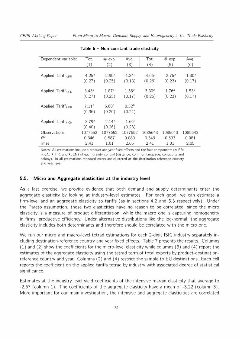
CEPII Working Paper From Micro to Macro: Demand, Supply, and Heterogeneity in the Trade Elasticity
Table 6 – Non-constant trade elasticity
Dependent variable: Tot. # exp. Avg. Tot. # exp. Avg.(1) (2) (3) (4) (5) (6)
Applied Tariffn,FR -4.25a -2.90a -1.34a -4.06a -2.76a -1.30a
(0.27) (0.25) (0.18) (0.26) (0.23) (0.17)
Applied Tariffn,CN 3.43a 1.87a 1.56a 3.30a 1.76a 1.53a
(0.27) (0.25) (0.17) (0.26) (0.23) (0.17)
Applied Tariffk,FR 7.11a 6.60a 0.52b
(0.36) (0.20) (0.24)
Applied Tariffk,CN -3.79a -2.14a -1.66a
(0.40) (0.26) (0.23)Observations 1077652 1077652 1077652 1085643 1085643 1085643R2 0.346 0.587 0.080 0.349 0.593 0.081rmse 2.41 1.01 2.05 2.41 1.01 2.05Notes: All estimations include a product and year fixed effects and the four components (n,FR;n,CN; k,FR; and k,CN) of each gravity control (distance, common language, contiguity andcolony). In all estimations standard errors are clustered at the destination-reference countryand year level.
5.5. Micro and Aggregate elasticities at the industry level
As a last exercise, we provide evidence that both demand and supply determinants enter theaggregate elasticity by looking at industry-level estimates. For each good, we can estimate afirm-level and an aggregate elasticity to tariffs (as in sections 4.2 and 5.3 respectively). Underthe Pareto assumption, those two elasticities have no reason to be correlated, since the microelasticity is a measure of product differentiation, while the macro one is capturing homogeneityin firms’ productive efficiency. Under alternative distributions like the log-normal, the aggregateelasticity includes both determinants and therefore should be correlated with the micro one.
We run our micro and macro-level tetrad estimations for each 2-digit ISIC industry separately in-cluding destination-reference country and year fixed effects. Table 7 presents the results. Columns(1) and (2) show the coefficients for the micro-level elasticity while columns (3) and (4) report theestimates of the aggregate elasticity using the tetrad term of total exports by product-destination-reference country and year. Columns (2) and (4) restrict the sample to EU destinations. Each cellreports the coefficient on the applied tariffs tetrad by industry with associated degree of statisticalsignificance.
Estimates at the industry level yield coefficients of the intensive margin elasticity that average to-2.67 (column 1). The coefficients of the aggregate elasticity have a mean of -3.22 (column 3).More important for our main investigation, the intensive and aggregate elasticities are correlated
31

CEPII Working Paper From Micro to Macro: Demand, Supply, and Heterogeneity in the Trade Elasticity
(pairwise correlations are .68 for the full sample, and .74 for the EU one). Figure 10 shows graph-ical evidence of those correlations that exhibits overwhelming evidence in favor of the aggregateelasticity including demand side determinants.
Table 7 – Micro and Aggregate elasticities by industry: 2000-2006
Micro AggregateDependent variable: firm-level exports total exports
(1) (2) (3) (4)Full EU Full EU
Agriculture -4.85a -3.77 -4.66a -4.9c
Food -2.1a -3.09a -3a -3.57a
Textile -1.85a -5.74a -1.84a -2.97b
Wearing -3.2a -3.23a -3.4a -3.64a
Leather -4.13a -5.96a -6.84a -8.72a
Wood -9.4a -20.88a -9.59a -15.33a
Paper 8.39a 6.35 6.64b 8.34Edition 1.68 2.2 5.02b 3.86Coke prod .02 1.39 .93 1.21Chemical -4.99a -7.29a -5.64a -7.66a
Rubber 5.12a 4.8a 12.18a 16.25a
Basic metal -4.55a -7.35a -3.17c -6.27c
Metal products -2.9a -6.33a -1.11c -3.32a
Machinery -3.18a -6.92a -2.89a -5.06a
Office -.06 -4.88 -21.14a -31.42b
Electrical Prod -2.49b -8.44a -.59 -1.34Equip. Radio, TV -8.38a -10.66a -7.08a -8.1a
Medical instruments -2.36a -3.9b -.38 -.29Vehicles -4.14c 12.69c -5.38a 15.52a
Transport -11.34a -18.28a -16.15a -17.37a
Furniture -1.35b -3.75a .26 0Notes: All estimations are run by industry 2 digit. The cells report thecoefficient on the applied tariffs tetrad by industry. All estimationsinclude destination-reference country and year fixed effects. Stan-dard errors are clustered by product-reference country and year. Allestimations include a constant that is not reported. Applied tariff isthe tetradic term of the logarithm of applied tariff plus one. a, b andc denote statistical significance levels of one, five and ten percentrespectively.
32

CEPII Working Paper From Micro to Macro: Demand, Supply, and Heterogeneity in the Trade Elasticity
Figure 10 – Aggregate and intensive margin elasticities by industry 2 digit
Agriculture
FoodTextile
WearingLeather
Wood
Paper
Edition
Coke prod
Chemical
Rubber
Basic metal
Metal productsMachinery
Office
Electrical Prod
Equip. Radio, TV
Medical instruments
Vehicles
Transport
Furniture
-15
-10
-50
510
15M
icro
ela
stic
ity (
1-s)
-30 -20 -10 0 10Aggregate elasticity (e)
Agriculture
FoodTextile
Wearing
Leather
Wood
ChemicalBasic metal
Metal productsMachinery
Equip. Radio, TV
Vehicles
Transport
-15
-10
-50
Mic
ro e
last
icity
(1-
s)
-20 -15 -10 -5 0Aggregate elasticity (e)
(a) Full set (b) Coeff sig. < 0
6. Conclusion
We have argued in this paper that knowledge of the firm-level response to trade costs is a centralelement to our understanding of aggregate export reaction. In other words, we need micro-leveldata to understand the macro-level impacts of trade costs, a central element in any trade policyevaluation. This need for micro data is presumably true with the vast majority of possible hetero-geneity distribution assumptions. There is one exception however where micro data is not neededto estimate the aggregate elasticity: the (untruncated) Pareto distribution. It is an exceptionthe literature has been concentrating on for reasons of tractability that are perfectly legitimate,but the evidence presented in our paper points to systematic variation in bilateral aggregate tradeelasticities that is both substantial and compatible with log-normal heterogeneity (in addition to bestrongly preferred when looking at the micro-level distribution of export sales). We therefore callfor a “micro approach” to estimating those elasticities as opposed to the “macro approach” usinggravity specified so as to estimate a constant elasticity.
The micro- and macro- approaches differ substantially in several respects. On the one hand,gravity is a more direct and parsimonious route for estimating aggregate elasticities: (i) parametricassumptions are reduced to a minimum while our micro-based procedure depends on the calibrationof the productivity distribution; (ii) gravity is less demanding in terms of data and makes possiblethe use of easily accessible dataset of bilateral aggregate trade flows. On the other hand, gravityprovides, for each origin country, only a cross-destination average of elasticities while the micro-based approach provides the full cross-dyadic distribution of elasticities. Given this last limitation,we use our gravity estimates of averaged elasticities as a benchmark for discriminating between the
33

CEPII Working Paper From Micro to Macro: Demand, Supply, and Heterogeneity in the Trade Elasticity
two distributional assumptions made in our micro-based quantifications. We find that average valueof bilateral trade elasticities obtained under a log-normal calibration is very close to the empiricalgravity estimate which constrains the elasticity to be constant across country pairs. By contrast,the Pareto-based calibration leads to predictions that seem invalidated by the data. Namely, theinvariance of average shipments to ad-valorem tariff variations, the lack of correlation between firm-level and aggregate level of elasticities estimated industry by industry, and the constant aggregatetrade elasticities.
References
Anderson, J. E. and van Wincoop, E. (2003). Gravity with gravitas: A solution to the borderpuzzle. American Economic Review, 93 (1):170–192.
Arkolakis, C. (2010). Market penetration costs and the new consumers margin in internationaltrade. Journal of Political Economy, 118(6):1151 – 1199.
Arkolakis, C., Costinot, A., and Rodríguez-Clare, A. (2010). Gains from trade under monopolisticcompetition: A simple example with translog expenditure functions and pareto distributions offirm-level productivity. manuscript.
Arkolakis, C., Costinot, A., and Rodriguez-Clare, A. (2012). New trade models, same old gains?American Economic Review, 102(1):94–130.
Atkeson, A. and Burstein, A. (2008). Pricing-to-market, trade costs, and international relativeprices. The American Economic Review, 98(5):1998–2031.
Baier, S. and Bergstrand, J. H. (2001). The growth of world trade: tariffs, transport costs, andincome similarity. Journal of International Economics, 53 (1):1–27.
Barba Navaretti, G., Bugamellli, M., Forlani, E., and Ottaviano, G. (2015). It takes (more than)a moment: Revisiting the link between firm productivity and aggregate exports. University ofMilan Mimeo.
Berman, N., Martin, P., and Mayer, T. (2012). How do different exporters react to exchange ratechanges? The Quarterly Journal of Economics, 127 (1):437–492.
Berthou, A. and Fontagné, L. (2015). Variable trade costs, composition effects, and the intensivemargin of trade. Technical Report 543, Banque de France.
Broda, C. and Weinstein, D. (2006). Globalization and the gains from variety. Quarterly Journalof Economics, 121 (2):541–585.
Caliendo, L. and Parro, F. (2015). Estimates of the trade and welfare effects of nafta. Review ofEconomic Studies, 82(1):1–44.
Chaney, T. (2008). Distorted gravity: The intensive and extensive margins of international trade.American Economic Review, 98 (4):1707–1721.
Costinot, A., Donaldson, D., and Komunjer, I. (2012). What goods do countries trade? a quanti-tative exploration of ricardo’s ideas. Review of Economic Studies, 79(2):581–608.
34

CEPII Working Paper From Micro to Macro: Demand, Supply, and Heterogeneity in the Trade Elasticity
Crozet, M., Head, K., and Mayer, T. (2012). Quality sorting and trade: Firm-level evidence forfrench wine. Review of Economic Studies, 79(2):609 – 644.
Eaton, J. and Kortum, S. (2001). Trade in capital goods. European Economic Review, 45(7):1195–1235.
Eaton, J. and Kortum, S. (2002). Technology, geography, and trade. Econometrica, 70 (5):1741–1779.
Eaton, J., Kortum, S., and Kramarz, F. (2011). An anatomy of international trade: Evidence fromFrench firms. Econometrica, 79(5):1453–1498.
Feenstra, R. C. (1994). New product varieties and the measurement of international prices. Amer-ican Economic Review, 84:157–177.
Feenstra, R. C. (2003). A homothetic utility function for monopolistic competition models. Eco-nomics Letters, 78(2):79–86.
Feenstra, R. C. (2013). Restoring the product variety and pro-competitive gains from trade withheterogeneous firms and bounded productivity. UC Davis Mimeo.
Fitzgerald, D. and Haller, S. (2014). Exporters and shocks: Dissecting the international elasticitypuzzle. manuscript.
Freund, C. and Pierola, M. D. (2015). Export superstars. Review of Economics and Statistics.
Hallak, J. C. (2006). Product quality and the direction of trade. Journal of International Economics,68 (1):238–265.
Harrigan, J. and Deng, H. (2010). ChinaâĂŹs local comparative advantage. In Feenstra, R. C.and Wei, S.-J., editors, ChinaâĂŹs Growing Role in World Trade, NBER Conference volume,volume 3. Chicago University.
Head, K. and Mayer, T. (2014). Gravity equations: Workhorse, toolkit, and cookbook. In Helpman,E., Gopinath, G., and Rogoff, K., editors, Handbook of International Economics, volume 4.Elsevier.
Head, K., Mayer, T., and Ries, J. (2010). The erosion of colonial trade linkages after independence.Journal of International Economics, 81 (1):1–14.
Head, K., Mayer, T., and Thoenig, M. (2014). Welfare and trade without pareto. AmericanEconomic Review, 104(5):310–16.
Head, K. and Ries, J. (2001). Increasing returns versus national product differentiation as anexplanation for the pattern of us-canada trade. American Economic Review, 91(4):858–876.
Helpman, E., Melitz, M., and Rubinstein, Y. (2008). Estimating trade flows: Trading partners andtrading volumes. Quarterly Journal of Economics, 123(2):441–487.
Hummels, D. (1999). Towards a geography of trade costs. Technical Report 17, GTAP WorkingPaper.
Imbs, J. and Méjean, I. (2014). Elasticity optimism. American Economic Journal: Macroeconomics.
Krugman, P. (1980). Scale economies, product differentiation, and the pattern of trade. AmericanEconomic Review, 70:950–959.
35

CEPII Working Paper From Micro to Macro: Demand, Supply, and Heterogeneity in the Trade Elasticity
Melitz, M. (2003). The impact of trade on intra-industry reallocations and agregate industryproductivity. Econometrica, 71:1695–1725.
Melitz, M. and Ottaviano, G. (2008). Market size, trade, and productivity. Review of EconomicStudies, 75(1):295–316.
Melitz, M. J. and Redding, S. J. (2015). New trade models, new welfare implications. AmericanEconomic Review.
Novy, D. (2013). International trade without CES: Estimating translog gravity. Journal of Inter-national Economics, 89(2):271–282.
Ossa, R. (2012). Why trade matters after all. Working Paper 18113, NBER.
Romalis, J. (2007). Nafta’s and cusfta’s impact on international trade. Review of Economics andStatistics, 89(3):416 – 435.
Simonovska, I. and Waugh, M. (2012). Different trade models, different trade elasticities?UC Davis and NYU Stern School of Business. Available at: http://www. econ. ucdavis.edu/faculty/sina/sw2.pdf.
Simonovska, I. and Waugh, M. E. (2011). The elasticity of trade: Estimates and evidence. WorkingPaper 16796, NBER.
Wooldridge, J. W. (2006). Cluster sample methods in applied econometrics: An extended analysis.Working paper, Michigan State University.
Yang, M.-J. (2014). Firm heterogeneity and trade in a distorted gravity world. University ofWashington Mimeo.
36

CEPII Working Paper From Micro to Macro: Demand, Supply, and Heterogeneity in the Trade Elasticity
Appendix
Appendix 8:. Empirical Appendix
A.8.1.. Descriptive statistics
Table A.1 – Average percentage point difference between the applied tariff to France and Chinaacross industries by Germany and Japan (2000)
Reference importer: Germany JapanFull Tetrad Full Tetrad
sample regression sample sample regression sample
Agriculture -3.27 -2.98 .01 .02Food -7.83 -9.63 1.24 1.45Textile -7.14 -6.95 5.31 4.58Wearing apparel -9.34 -8.11 6.2 6.79Leather -1.5 -1.15 8.4 4.68Wood -1.36 -1.47 2.66 3.69Paper 0 0 1.39 1.3Edition -.79 -.65 .26 .64Coke prod 0 0 .97 1.73Chemical -1.01 -.74 2.51 2.4Rubber & Plastic -1.37 -1.25 2.5 2.37Non Metallic -1.43 -2.18 1.16 .8Basic metal products -1.84 -3.56 1.89 2.75Metal products -.67 -.99 1.38 1.32Machinery -.25 -.3 .19 0Office -.16 -.38 0 0Electrical Prod -.38 -.47 .37 .62Equip. Radio, TV -1.72 -1.79 0 0Medical instruments -.58 -.41 .14 .34Vehicles -2.22 -1.63 0 0Transport -1.27 -1.37 0 0Furniture -.51 -.63 1.93 1.95
37

CEPII Working Paper From Micro to Macro: Demand, Supply, and Heterogeneity in the Trade Elasticity
Table A.2 – Destination countries characteristics in 2000
Ratio France / China:Population GDP Total Average Number Distance
exports exports exportersCHE 7 246 23.03 1.27 18.1 .06BEL 10 232 9.63 1.21 7.94 .06NLD 16 387 2.04 1.01 2.02 .08GBR 60 1443 4.89 2.37 2.06 .09ESP 40 581 14.37 3.82 3.76 .1DEU 82 1900 5.04 2.13 2.37 .1ITA 57 1097 7.32 2.71 2.71 .11AUT 8 194 10.68 1.83 5.83 .12IRL 4 96 8.52 1.38 6.19 .12CZE 10 57 5.56 2.48 2.24 .13PRT 10 113 17.95 1.98 9.07 .13DNK 5 160 3.15 1.07 2.94 .16MAR 28 33 10.08 1.57 6.43 .16POL 38 171 3.93 1.68 2.34 .18MLT 0 4 8.29 5.18 1.6 .18SWE 9 242 5.91 2.66 2.22 .22NOR 4 167 2.47 1.66 1.49 .22BGR 8 13 4.31 2.19 1.97 .24GRC 11 115 4.41 1.75 2.52 .24BLR 10 13 1.19 .22 5.29 .28MDA 4 1 97.59 6.15 15.88 .28EST 1 6 1.39 .45 3.07 .3FIN 5 121 1.9 .87 2.2 .32GHA 20 5 1.06 1.99 .53 .38NGA 125 46 1.15 2.32 .5 .38CYP 1 9 1.43 1.27 1.13 .39LBN 4 17 3.19 2.06 1.55 .43JOR 5 8 .92 2.31 .4 .45GAB 1 5 78.18 2.17 36.09 .46BRB 0 3 2.01 1.79 1.12 .47SUR 0 1 1.38 5.22 .26 .47ATG 0 1 5.22 1.08 4.82 .48GUY 1 1 1.42 8.22 .17 .48VCT 0 0 4.19 .98 4.27 .48BRA 174 644 1.77 1.87 .94 .5VEN 24 117 1.23 2.51 .49 .52DOM 9 20 1.21 1.58 .77 .52PRY 5 7 .31 1.18 .27 .54BOL 8 8 2.89 2.36 1.22 .55JAM 3 8 1.38 5.35 .26 .56URY 3 21 .59 2.1 .28 .57COL 42 84 1.66 2.36 .7 .57ARG 37 284 1.72 2.94 .59 .57CUB 11 . 1.04 1.41 .74 .58PER 26 53 .82 1.97 .42 .6PAN 3 12 .09 1.14 .08 .6CHL 15 75 1.12 4.23 .27 .61UGA 24 6 2.74 3.98 .69 .62CRI 4 16 1.4 3.95 .35 .62CAN 31 714 .73 1.51 .48 .62SAU 21 188 1.21 2.52 .48 .62NIC 5 4 .19 .74 .25 .63HND 6 6 .39 1.56 .25 .64SLV 6 13 3.86 11.98 .32 .65GTM 11 19 .25 1 .25 .67USA 282 9765 .54 1.13 .48 .67KEN 31 13 1.09 2.14 .51 .68YEM 18 9 .83 3.39 .25 .7TZA 34 9 .28 1.26 .22 .71IRN 64 101 1 1.56 .64 .72MEX 98 581 .93 1.31 .71 .75SYC 0 1 19.33 8.66 2.23 .98LKA 19 16 1.2 7.96 .15 1.72NZL 4 53 .54 1.96 .28 1.84AUS 19 400 .38 1.73 .22 1.98NPL 24 5 .08 .42 .2 2.24IDN 206 165 .12 .94 .12 2.47BGD 129 47 .14 1.91 .07 2.7THA 61 123 .32 1.04 .31 3.17BRN 0 4 .58 3.05 .19 3.22LAO 5 2 .25 .69 .36 3.83PHL 76 76 .4 2.49 .16 4.21JPN 127 4650 .12 .6 .19 4.96TWN 22 321 .35 1.32 .26 6.69Notes: Population is expressed in millions and GDP in billions of US dollars.
38

CEPII Working Paper From Micro to Macro: Demand, Supply, and Heterogeneity in the Trade Elasticity
Table A.3 – Avg. difference between tariffs applied to France and China. Full sample
France < China France = China France > ChinaTariff # HS6 Tariff # HS6 Tariff # HS6
ARG . 0 0 5113 . 0ATG . 0 0 5097 . 0AUS . 0 0 4188 1.91 905AUT -5.7 2137 0 2825 . 0BEL -5.7 2137 0 2825 . 0BGD . 0 0 5106 . 0BGR . 0 0 5059 . 0BLR . 0 0 4559 . 0BOL . 0 0 5113 . 0BRA . 0 0 5113 . 0BRB . 0 0 2020 . 0BRN . 0 0 5079 . 0CAN -3.87 15 0 2877 3.07 2178CHE -10 1 0 4120 . 0CHL . 0 0 5113 . 0COL . 0 0 5113 . 0CRI . 0 0 5113 . 0CUB . 0 0 5112 . 0CYP . 0 0 4929 . 0CZE . 0 0 5113 . 0DEU -5.7 2137 0 2825 . 0DNK -5.7 2137 0 2825 . 0DOM . 0 0 5008 . 0ESP -5.7 2137 0 2825 . 0EST . 0 0 5113 . 0FIN -5.7 2137 0 2825 . 0GAB . 0 0 5108 . 0GBR -5.7 2137 0 2825 . 0GHA . 0 0 5019 . 0GRC -5.7 2137 0 2825 . 0GTM . 0 0 5113 . 0GUY . 0 0 2043 . 0HND . 0 0 5113 . 0IDN . 0 0 5110 . 0IRL -5.7 2137 0 2825 . 0IRN . 0 0 5113 . 0ITA -5.7 2137 0 2825 . 0JAM . 0 0 5113 . 0JOR . 0 0 5085 . 0JPN -.18 3 0 2771 4.06 2256KEN . 0 0 4554 . 0LAO . 0 0 4977 . 0LBN . 0 0 5067 . 0LKA . 0 0 5090 . 0MAR . 0 0 5113 . 0MDA . 0 0 5068 . 0MEX . 0 0 5084 . 0MLT . 0 0 5109 . 0NGA . 0 0 5113 . 0NIC . 0 0 5113 . 0NLD -5.7 2137 0 2825 . 0NOR -10.74 1210 0 3560 . 0NPL . 0 0 5096 . 0NZL . 0 0 3220 1.15 1876PAN . 0 0 5110 . 0PER . 0 0 5113 . 0PHL . 0 0 5112 . 0POL -9.51 4234 0 485 7.14 388PRT -5.7 2137 0 2825 . 0PRY . 0 0 5113 . 0SAU . 0 0 4799 . 0SLV . 0 0 5113 . 0SUR . 0 0 1170 . 0SWE -5.7 2137 0 2825 . 0SYC . 0 0 4849 . 0THA . 0 0 5056 . 0TWN . 0 0 5113 . 0TZA . 0 0 5113 . 0UGA . 0 0 5110 . 0URY . 0 0 4829 . 0USA . 0 0 4768 . 0VCT . 0 0 2040 . 0VEN . 0 0 5109 . 0YEM . 0 0 5111 . 0Notes: The table reports the average difference across hs6 products of applied tariffsby destination country n to France and China and the corresponding number of hs6products when the tariff applied to France is lower than to China (columns (1) and(2)), when the applied tariff to both origin countries is the equal (columns (3) and(4)) and when the tariff applied to France is higher than to China (columns (5) and(6)).
39

CEPII Working Paper From Micro to Macro: Demand, Supply, and Heterogeneity in the Trade Elasticity
Table A.4 – Avg. difference between tariffs applied to France and China. Tetrad sample.
France < China France = China France > ChinaTariff # HS6 Tariff # HS6 Tariff # HS6
ARG . 0 0 567 . 0ATG . 0 0 1 . 0AUS . 0 0 816 1.87 249AUT -6.06 357 0 377 . 0BEL -5.43 651 0 772 . 0BGD . 0 0 73 . 0BGR . 0 0 121 . 0BLR . 0 0 9 . 0BOL . 0 0 11 . 0BRA . 0 0 636 . 0BRB . 0 0 5 . 0BRN . 0 0 6 . 0CAN . 0 0 424 2.78 571CHE -10 1 0 658 . 0CHL . 0 0 419 . 0COL . 0 0 183 . 0CRI . 0 0 37 . 0CUB . 0 0 25 . 0CYP . 0 0 255 . 0CZE . 0 0 434 . 0DEU -5.58 831 0 982 . 0DNK -5.74 465 0 500 . 0DOM . 0 0 56 . 0ESP -5.41 720 0 859 . 0EST . 0 0 52 . 0FIN -5.47 367 0 412 . 0GAB . 0 0 24 . 0GBR -5.55 802 0 964 . 0GHA . 0 0 37 . 0GRC -5.37 446 0 556 . 0GTM . 0 0 51 . 0GUY . 0 0 2 . 0HND . 0 0 19 . 0IDN . 0 0 457 . 0IRL -5.32 257 0 291 . 0IRN . 0 0 162 . 0ITA -5.43 760 0 895 . 0JAM . 0 0 17 . 0JOR . 0 0 206 . 0JPN -.01 1 0 631 4.09 535KEN . 0 0 74 . 0LAO . 0 0 1 . 0LBN . 0 0 401 . 0LKA . 0 0 128 . 0MAR . 0 0 407 . 0MDA . 0 0 3 . 0MEX . 0 0 533 . 0MLT . 0 0 130 . 0NGA . 0 0 116 . 0NIC . 0 0 5 . 0NLD -5.64 748 0 920 . 0NOR -8.03 267 0 248 . 0NPL . 0 0 15 . 0NZL . 0 0 189 1.09 308PAN . 0 0 125 . 0PER . 0 0 119 . 0PHL . 0 0 420 . 0POL -9.6 564 0 41 8.1 9PRT -4.78 396 0 426 . 0PRY . 0 0 45 . 0SAU . 0 0 512 . 0SLV . 0 0 27 . 0SUR . 0 0 1 . 0SWE -5.94 489 0 511 . 0SYC . 0 0 1 . 0THA . 0 0 662 . 0TWN . 0 0 864 . 0TZA . 0 0 13 . 0UGA . 0 0 6 . 0URY . 0 0 180 . 0USA . 0 0 1809 . 0VCT . 0 0 1 . 0VEN . 0 0 258 . 0YEM . 0 0 59 . 0Notes: The table reports the average difference across hs6 products of applied tariffsby destination country n to France and China and the corresponding number of hs6products when the tariff applied to France is lower than to China (columns (1) and(2)), when the applied tariff to both origin countries is the equal (columns (3) and(4)) and when the tariff applied to France is higher than to China (columns (5) and(6)).
40

CEPII Working Paper From Micro to Macro: Demand, Supply, and Heterogeneity in the Trade Elasticity
A.8.2.. Alternative specifications of the intensive margin estimates
A.8.2.1.. Identification across products
Estimations on the intensive margin trade elasticity in the main text exploit variation of appliedtariffs within hs6 products across destination countries and exporters (firms located in France andChina). This section presents a set of estimations on alternative specifications that exploits thevariation of applied tariffs within destination countries across hs6-products.
Table A.5 reports the results from estimations including a destination-reference importer countryfixed effect. In this case, standard errors are clustered by hs6-reference importer country. Includingthese fixed effects implies that the source of identification comes from variations within destinationcountries across hs6-products in applied tariffs to both origin countries, France and China, by thereference importer countries. Columns (1) and (3) present estimations on the full sample, whilecolumns (2) and (4) report estimations on the sample of positive tetraded tariffs. The tradeelasticity ranges from -3.57 to -5.07. Estimations in columns (5) and (6) restrict the destinationcountries to be the ones applying non-MFN duties and in column (7) to EU destination countriesincluding countries with EU-trade agreements as Norway and Switzerland. The sample size dropsradically, with the trade elasticities remaining of the expected sign and order of magnitude, butlosing in statistical significance.
Table A.5 – Intensive margin elasticities. Within-country estimations.
Top 1 Top 1 to 10Dependent variable: firm-level exports firm-level exportsSample: Full Full non-MFN EU
(1) (2) (3) (4) (5) (6) (7)
Applied Tariff -3.53a -3.59a -3.10a -5.07a -2.93a -5.28a -2.48a
(1.07) (1.26) (0.70) (0.83) (0.83) (0.94) (0.61)Observations 37396 15477 99645 41376 12992 9421 54198R2 0.001 0.002 0.001 0.003 0.001 0.004 0.000rmse 2.92 2.93 3.02 3.05 3.09 3.06 2.95Notes: All estimations include destination-reference importing country fixed effects Standarderrors are clustered by hs6-reference importing country. Applied tariff is the tetradic term ofthe logarithm of applied tariff plus one. Columns (5) and (6) present the estimations for thenon-MFN sample. Columns (2), (4) and (6) present estimations on the sample of positivetetraded tariffs. a, b and c denote statistical significance levels of one, five and ten percentrespectively.
A.8.2.2.. Cross-section estimations in 2001 and 2006
Results in the main text focus on cross-sectional analysis of the year 2000 (before entry of Chinainto WTO). We now turn to additional cross-section evidence after China entry into WTO (2001)
41

CEPII Working Paper From Micro to Macro: Demand, Supply, and Heterogeneity in the Trade Elasticity
and for the final year of our sample (2006), in Table A.6. Estimations in columns (1) and (3)include a fixed effect identifying the product-reference country combination while columns (2) and(4) include a fixed effect identifying the destination-reference importing country. As expectedthe coefficients on tariffs are lower since the difference of tariffs applied to France and China bydestination countries is reduced after 2001. The implied values of σ range from -3.6 to almost -2.
Table A.6 – Intensive margin: cross-section 2001 and 2006
Dependent variable: Top 1 to 10 firm-level exports2001 2006
(1) (2) (3) (4)
Applied Tariff -1.83a -2.59a -0.95b -1.42b
(0.64) (0.68) (0.42) (0.61)
Distance -0.62a -0.54a
(0.02) (0.02)
Contiguity 0.75a 0.98a
(0.08) (0.06)
Colony -0.02 0.49a
(0.09) (0.07)
Common language -0.13b -0.03(0.06) (0.05)
Observations 111039 111039 217732 217732R2 0.129 0.000 0.107 0.000rmse 2.46 3.04 2.45 2.96Notes: Estimations in columns (1) and (3) include a fixed effectidentifying the hs6 product-reference importing country and stan-dard errors are clustered by destination-reference importer country.Estimations in columns (2) and (4) include a fixed effect identifyingthe destination-reference importing country and standard errors areclustered by hs6 product-reference importer country. Applied tariff isthe tetradic term of the logarithm of applied tariff plus one. a, b andc denote statistical significance levels of one, five and ten percentrespectively.
A.8.2.3.. Panel estimations 2000-2006
Our dataset spans over the 2000-2006 period. This dimension allows to identify the variationof tariffs within product-destination over time and across reference countries. Table A.7 reports
42

CEPII Working Paper From Micro to Macro: Demand, Supply, and Heterogeneity in the Trade Elasticity
results. Columns (1) and (3) present the baseline estimation for the 2000-2006 period, columns(2) and (5) present estimations on the sample of non-MFN destinations and columns (3) and (6)on the sample of EU destination countries. All estimations include product-destination, year andimporting reference country fixed effects. The coefficients of the intensive margin elasticity areclose to the findings from the cross-section estimations of 2000, and they range from -5.26 to-1.80.
Table A.7 – Intensive margin elasticities. Within-product-destination country estimations 2000-2006
Top 1 Top 1 to 10Dependent variable: firm-level exports firm-level exports
(1) (2) (3) (4) (5) (6)
Applied Tariff -3.20a -2.47a -5.26a -1.99a -1.80a -3.66a
(0.40) (0.62) (0.57) (0.25) (0.39) (0.36)
Distance -0.38a -0.44a -0.28a -0.45a -0.51a -0.35a
(0.01) (0.02) (0.01) (0.01) (0.01) (0.01)
Contiguity 0.28a 0.23a 0.31a 0.53a 0.52a 0.31a
(0.03) (0.04) (0.03) (0.02) (0.03) (0.02)
Common language -0.31a -0.44a -0.24a -0.24a -0.35a -0.11a
(0.04) (0.05) (0.05) (0.03) (0.03) (0.03)Observations 379644 61882 198629 1077652 167758 558424R2 0.081 0.099 0.060 0.085 0.109 0.060rmse 2.23 2.11 2.27 2.48 2.37 2.50Notes: All estimations include hs6-destination country, reference importing country and yearfixed effects. Standard errors are clustered by destination-reference importing country andyear. Applied tariff is the tetradic term of the logarithm of applied tariff plus one. Columns(2) and (5) present estimations on the sample of non-MFN destinations and columns (3) and(6) on the sample of EU destination countries. a, b and c denote statistical significance levelsof one, five and ten percent respectively.
A.8.3.. Selection bias
Not all firms export to all markets n, and the endogenous selection into different export destinationsacross firms is one of the core elements of the type of model we are using. To understand thepotential selection bias associated with estimating the trade elasticity it is useful to recall the firm-level export equation (3), now accounting for the fact that we have exporters from both China andFrance, and therefore using the export country index i :
ln xni(α) = (1− σ) ln
(σ
σ − 1
)+ (1− σ) ln(αwi) + (1− σ) ln τni + lnAn + ln εni(α). (A.1)
43

CEPII Working Paper From Micro to Macro: Demand, Supply, and Heterogeneity in the Trade Elasticity
In this model, selection is due to the presence of a fixed export cost fni that makes some firmsunprofitable in some markets. Assuming that fixed costs are paid using labor of the origin country,profits in this setup are given by xni(α)/σ−wi fni , which means that a firm is all the more likely tobe present in market n that its (1−σ) ln(αwi) + (1−σ) ln τni + lnAn + ln εni(α) is high. Thereforea firm with a low cost (αwi) can afford having a low draw on εni(α), creating a systematic bias onthe cost variable. The same logic applies in attractive markets, (high An), which will be associatedwith lower average draws on the error term. Fortunately , our tetrad estimation technique removesthe need to estimate αwi and An, and therefore solves this issue.
However a similar problem arises with the trade cost variable, τni , which is used to estimate thetrade elasticity. Higher tariff countries will be associated with firms having drawn higher εni(α),thus biasing downwards our estimate of the trade elasticity. Our approach of tetrads that focuseson highly ranked exporters for each hs6-market combination should however not be too sensitiveto that issue, since those are firms that presumably have such a large productivity that theiridiosyncratic destination shock is of second order. In order to verify that intuition, we follow Eatonand Kortum (2001), applied to firm-level data by Crozet et al. (2012), who assume a normallydistributed ln εni(α), yielding a generalized structural tobit. This procedure uses the theoreticalequation for minimum sales, xMINni (α) = σwi fni , which provides a natural estimate for the truncationpoint for each desination market. This method (EK tobit) keeps all individual exports to all possibledestination markets (including zeroes).24 When estimating equation (A.1), we proxy for lnAn withGDPn and populationn, and for firm-level determinants α with the count of markets served by thefirm. An origin country dummy for Chinese exporters account for all differences across the twogroups, such as wages, wi . Last, we ensure comparability by i) keeping the same sample of product-market combinations as in previous estimations using tetrads, ii) running the estimation with thesame dimension of fixed effects (hs6). Each column of Tables A.8 and A.9 show the simple OLS(biased) estimates or the EK-tobit method run in the sample of product-market combinations byreference importing country. As in previous usages of that method, the OLS seems very severelybiased, probably due to the extremely high selection levels observed (with all reference countries,slightly less than 14% of possible flows are observed). Strikingly, the EK tobit estimates are verycomparable to the tetrad estimates shown until now , giving us further confidence in an order ofmagnitude of the firm-level trade elasticity around located between -4 and -6.25
24For each product, we fill in with zero flows destinations that a firm found unprofitable to serve in reality. The set ofpotential destinations for that product is given all countries where at least one firm exported that good.25Pooling over all the reference countries gives tariff elasticities of 1.893 for OLS and -4.925 for the EK tobit, bothvery significant. This pattern and those values are very much in line with detailed results from Tables A.8 and A.9.
44

CEPII Working Paper From Micro to Macro: Demand, Supply, and Heterogeneity in the Trade Elasticity
Table A.8 – Correcting for the selection bias.
(1) (2) (3) (4) (5) (6) (7) (8)Ref. country: Australia Canada Germany Italy
OLS EK Tobit OLS EK Tobit OLS EK Tobit OLS EK Tobit
Applied Tariff 1.26a -6.28a 1.33a -5.05a 2.09a -3.78a 1.41a -6.39a
(0.16) (0.87) (0.18) (0.93) (0.17) (0.71) (0.16) (0.74)
RTA -0.67a 1.37a -0.55a 2.36a -0.63a 2.27a -0.67a 2.42a
(0.06) (0.33) (0.06) (0.34) (0.06) (0.31) (0.05) (0.30)
Distance 0.01 -0.40a 0.05b 0.14 0.02 -0.21c 0.04b -0.06(0.02) (0.13) (0.02) (0.12) (0.02) (0.11) (0.02) (0.11)
Common language 0.07c 3.32a 0.30a 4.95a 0.21a 3.94a 0.22a 4.14a
(0.04) (0.20) (0.04) (0.23) (0.03) (0.17) (0.03) (0.17)
Contiguity 0.07b 1.55a 0.06b 1.23a 0.15a 1.91a 0.10a 1.85a
(0.03) (0.12) (0.03) (0.12) (0.02) (0.10) (0.02) (0.11)
Colony 0.64a 4.29a 0.69a 2.50a 0.85a 2.65a 0.79a 2.23a
(0.10) (0.55) (0.10) (0.55) (0.09) (0.43) (0.08) (0.43)
GDPn 0.16a 1.57a 0.15a 1.84a 0.19a 1.65a 0.16a 1.48a
(0.01) (0.05) (0.01) (0.06) (0.01) (0.05) (0.01) (0.05)
Populationn 0.03b 0.71a 0.07a 0.61a 0.02 0.67a 0.04a 0.84a
(0.01) (0.06) (0.02) (0.07) (0.01) (0.05) (0.01) (0.06)
Chinese exporter dummy 0.26a 0.44a 0.39a 0.58a 0.51a 1.44a 0.37a 1.11a
(0.03) (0.13) (0.04) (0.16) (0.03) (0.15) (0.03) (0.14)
# of dest. by firm 0.19a 2.06a 0.14a 1.98a 0.13a 1.96a 0.14a 2.04a
(0.01) (0.03) (0.01) (0.03) (0.01) (0.03) (0.01) (0.03)Observations 617231 5518719 571508 4386238 730720 5828685 735346 5917116R2 0.058 0.051 0.059 0.053Pseudo R2 0.082 0.086 0.075 0.077Notes: All estimations include fixed effects for each hs6 product level. Standard errors are clustered at the hs6-destination-origin country level. Applied tariff is the logarithm of applied tariff plus one at the hs6 product level anddestination country. a, b and c denote statistical significance levels of one, five and ten percent respectively.

CEPII Working Paper From Micro to Macro: Demand, Supply, and Heterogeneity in the Trade Elasticity
Table A.9 – Correcting for the selection bias.(cont.)
(1) (2) (3) (4) (5) (6) (7) (8)Ref. country: Japan UK New Zealand Poland
OLS EK Tobit OLS EK Tobit OLS EK Tobit OLS EK Tobit
Applied Tariff 1.13a -5.45a 1.73a -4.99a 0.62a -4.34a 1.22a -4.60a
(0.23) (1.09) (0.16) (0.78) (0.22) (1.14) (0.20) (0.87)
RTA -0.28a 3.12a -0.73a 2.62a -0.51a 1.65a -0.52a 1.98a
(0.08) (0.37) (0.05) (0.29) (0.08) (0.40) (0.08) (0.35)
Distance 0.18a 0.38a 0.05a -0.08 0.07b -0.18 0.08a -0.03(0.03) (0.13) (0.02) (0.11) (0.03) (0.14) (0.03) (0.12)
Common language 0.28a 3.70a 0.25a 4.31a 0.31a 4.01a 0.25a 4.21a
(0.04) (0.20) (0.03) (0.16) (0.06) (0.29) (0.05) (0.24)
Contiguity 0.02 1.46a 0.14a 1.31a 0.03 1.67a 0.09b 1.75a
(0.03) (0.13) (0.02) (0.11) (0.04) (0.19) (0.04) (0.16)
Colony 0.56a 3.91a 0.73a 2.51a 0.64a 4.17a 0.71a 3.41a
(0.11) (0.79) (0.08) (0.51) (0.11) (0.98) (0.09) (0.57)
GDPn 0.13a 1.71a 0.17a 1.57a 0.14a 1.80a 0.19a 1.58a
(0.01) (0.07) (0.01) (0.05) (0.02) (0.08) (0.02) (0.07)
Populationn 0.09a 0.73a 0.03b 0.71a 0.08a 0.52a 0.02 0.59a
(0.02) (0.08) (0.01) (0.06) (0.02) (0.09) (0.02) (0.07)
Chinese exporter dummy 0.21a 1.10a 0.40a 1.40a 0.15a 0.10 0.34a 1.08a
(0.04) (0.15) (0.03) (0.14) (0.04) (0.20) (0.05) (0.18)
# of dest. by firm 0.18a 1.91a 0.14a 1.95a 0.25a 2.43a 0.22a 2.18a
(0.01) (0.03) (0.01) (0.03) (0.01) (0.05) (0.01) (0.04)Observations 414135 2732178 735485 5901262 343141 2864115 361503 2891673R2 0.046 0.061 0.048 0.052Notes: All estimations include fixed effects for each hs6 product level. Standard errors are clustered at the hs6-destination-origin country level. Applied tariff is the logarithm of applied tariff plus one at the hs6 product level anddestination country. a, b and c denote statistical significance levels of one, five and ten percent respectively.

CEPII Working Paper From Micro to Macro: Demand, Supply, and Heterogeneity in the Trade Elasticity
A.8.4.. Non-constant trade elasticity
Table A.10 – Non-constant trade elasticity
2000 2006Dependent variable: Tot. # exp. Avg. Tot. # exp. Avg.
(1) (2) (3) (4) (5) (6)
Applied Tariffn,FR -5.74a -3.41a -2.34a -4.31a -3.52a -0.79b
(1.02) (0.69) (0.72) (0.53) (0.57) (0.37)
Applied Tariffn,CN 5.08a 2.55a 2.53a 2.16a 1.55a 0.61(0.99) (0.71) (0.66) (0.57) (0.58) (0.38)
Observations 99745 99745 99745 218036 218036 218036R2 0.357 0.590 0.093 0.339 0.594 0.072rmse 2.42 1.00 2.02 2.34 0.98 2.01Notes: All estimations include a product and reference country fixed effects and thefour components (nFR, nCN, kFR, and kCN) of each gravity control (distance, com-mon language, contiguity and colony). In all estimations standard errors are clusteredat the destination-reference country.
Appendix 9:. Theoretical Mean-to-Min ratios under Pareto and Log-Normal distributions
In general, the shape of the distribution of firms’ productivity matters for the aggregate tradeelasticity, generating heterogeneous responses across country pairs to the same trade costs shockIn this Appendix we consider two different distributions of the (rescaled) productivity: i) Pareto,which turns out to be a quite special case where heterogeneity washes out, and ii) Log-normal whichmaintains the mapping between heterogeneous productivity and heterogeneous trade elasticities.
More precisely, the central relationship (13) makes it clear that the heterogeneity of aggregatetrade elasticity comes entirely from the term γni that stems from endogenous selection of firmsinto export markets (see equation 14). In turn, γni depends on the cost-performance index Vnias defined by (11). We therefore need to understand how these γ and V terms behave underalternative distribution assumptions.
If productivity is Pareto then the rescaled unit input requirement a has PDF g(a) = θaθ−1/aθ,which translates into
V Pni =
θa∗θ−σ+1ni
aθ(θ − σ + 1). (A.2)
The elasticity of Vni with respect to a∗ is
γPni = θ − σ + 1 > 0. (A.3)
47

CEPII Working Paper From Micro to Macro: Demand, Supply, and Heterogeneity in the Trade Elasticity
Hence, Pareto makes all the γni terms be the same, and therefore transforms an expression generallyyielding heterogeneous trade elasticities into a one-parameter elasticity d lnXni
d ln τni= θ, that is related
to the supply side of the economy only.
When productive efficiency is distributed log-normally, things are very different. For ϕ ∼log-N (µ, ν), the distribution of rescaled unit input requirements is a ∼log-N (−µ, ν), and we canwrite
V LNni = exp[(σ − 1)µ+ (σ − 1)2ν2/2]Φ[(ln a∗ni + µ)/ν + (σ − 1)ν], (A.4)
where Φ() denotes the CDF of the standard normal distribution. Differentiating ln Vni with respectto ln a∗ni ,
γLNni =
1
νh
(ln a∗ni + µ
ν+ (σ − 1)ν
), (A.5)
where h(x) ≡ φ(x)/Φ(x), the ratio of the PDF to the CDF of the standard normal. Thus γniis no longer the constant 1 − σ + θ which obtains for productivity distibuted Pareto with shapeparameter θ.
The H function is a central element of our calibration procedure, as summarized by relationship(16) , that reveals cutoffs and therefore aggregate bilateral elasticities. Comparing (11), (14) and(15) we see that H and γ are closely related
γni ×H(a∗ni) = a∗nig(a∗ni)
G(a∗ni)(A.6)
With Pareto, we make use of (A.3) to obtain
HP(a∗ni) =θ
θ − σ + 1, (A.7)
With a log-normal productivity, equation (A.5) leads to
HLN(a∗ni) =h[(ln a∗ni + µ)/ν]
h[(ln a∗ni + µ)/ν + (σ − 1)ν], (A.8)
An attractive feature of our quantification procedure relates to the small number of relevant pa-rameters to be calibrated. Under Pareto, equations (A.3) and (A.7) show that only the shapeparameter θ matters. Similarly, under a log-normal, only the calibration of the second-moment ofthe distribution, ν, is necessary for inverting the H function to reveal the cutoff and for quantifyingthe aggregate elasticity: This last point stems from the fact that shifting the first moment, µ,affects (A.5) and (A.8) in an identical way and so has no impact on the quantification.
48

CEPII Working Paper From Micro to Macro: Demand, Supply, and Heterogeneity in the Trade Elasticity
Appendix 10:. Monte Carlo Simulations
In Section 5.3 we find that the macro-based estimate of the aggregate trade elasticity is quan-titatively close to the cross-dyadic average of the micro-based estimates when heterogeneity iscalibrated as being log-normal. We interpret this finding as an empirical support in favor of thisdistributional assumption. In this section we substantiate this last statement by embracing a moretheoretical perspective. This is an important step in the argument because the theoretical relation-ship between the macro- and the micro-based estimates of the elasticities is unknown (except underPareto where they are unambiguously equal). Hereafter we provide simulation-based evidence thatthe similarity between micro- and macro-based estimates is not accidental, even under log-normalheterogeneity.
We proceed with Monte Carlo (MC) simulations of our generic trade model with heterogeneousfirms. In the baseline simulations we generate fake bilateral trade for 10 countries and 1 millionactive firms per country. Our data generating process uses the firms’ sales in equation (2). Firm-level heterogeneity in terms of rescaled labor requirement, a ≡ α× b(α) is assumed to be Paretoor Log-normally distributed with a set of parameters identical to the ones used in our empiricalanalysis (section 5.2). We also retain σ = 5 as the parameter for the intensive margin. Withoutloss of generality, in this partial equilibrium framework, we normalize the nominal wage, w = 1,and we draw An/fni , i.e. the dyadic ratio of destination n attractiveness over entry cost from alog-normal distribution. This distribution is calibrated such as to match an average dyadic shareof exporting firms of 10 percent. Finally the applied-tariffs τni = 1 + tni are drawn from an uniformdistribution over the range [1, 2].
In each MC draw, we first generate a matrix of firm-level trade flows that are non-zero when salesexceed the bilateral entry cost, i.e. xni(a) > σwfni . In a first stage we infer from this fake tradedataset the micro-based estimates of the aggregate trade elasticities by applying the methodologyof Section 5.2: We first retrieve min-to-mean ratios for all country-pairs and then compute thecorresponding set of theoretical dyadic elasticities (equations 17 and 18). In a second stage, weturn to the macro-based estimates of the trade elasticity. To this purpose we collapse firm-leveltrade flows at the country-pair level to construct a matrix of bilateral aggregate trade. We then rungravity regressions (both using country fixed effects and tetrads) and retrieve the point estimate ofapplied tariffs. Hence, for each draw, we obtain one macro-based estimate of the trade elasticitythat we compare to the cross-dyadic average of the micro-based elasticities. This procedure isreplicated 50 times. Notice that it is computationally demanding as we have to manipulate verylarge trade matrices (1 million firms × 10 origin countries × 10 destination countries) .
The simulation results are displayed in Table A.11 for log-normal (col.1-col.4) and Pareto (col.5-col.8) and for different degrees of firm scarceness (from 1000 to 1 million firms per country). Eachcolumn reports averages and standard errors across replications.
Our baseline simulation under Pareto (col. 8) shows that the simulated economy with 1 millionfirms conforms to the theoretical prediction of a model with a continuum of firms. The micro-based
49

CEPII Working Paper From Micro to Macro: Demand, Supply, and Heterogeneity in the Trade Elasticity
Table A.11 – Monte Carlo results: elasticities wrt to a change in trade costs
Distribution: Log-Normal Pareto# firms per country: 1K 10K 100K 1M 1K 10K 100K 1M
total exports (micro) -4.69 -4.57 -4.56 -4.55 -5.74 -5.36 -5.23 -5.18(0.60) (0.38) (0.34) (0.33) (0.87) (0.37) (0.21) (0.13)
total exports (macro/tetrads) -4.80 -4.60 -4.59 -4.58 -5.55 -5.37 -5.21 -5.18(0.66) (0.29) (0.09) (0.03) (0.81) (0.56) (0.35) (0.22)
total exports (macro/FE) -4.65 -4.57 -4.55 -4.55 -5.59 -5.31 -5.22 -5.17(0.20) (0.09) (0.03) (0.01) (0.29) (0.16) (0.15) (0.08)
nb exporters (macro/FE) -3.20 -3.16 -3.16 -3.16 -5.19 -5.15 -5.14 -5.13(0.09) (0.03) (0.01) (0.00) (0.13) (0.05) (0.02) (0.01)
avg. exports (macro/FE) -1.45 -1.41 -1.40 -1.39 -0.40 -0.15 -0.08 -0.04(0.17) (0.08) (0.03) (0.01) (0.26) (0.16) (0.15) (0.08)
Notes: 50 replications for each cell, parameters on fixed costs of exports and size of the demand term havebeen calibrated so the share of exporters averages to 10-11% in all simulations. For each elasticity, the firstline reports the average value. Standard deviations are in parentheses. For the micro elasticity, the numberin parentheses is the average of standard deviations of the elasticity in each draw (quantifying the degree ofheterogeneity in bilateral elasticities). For the macro elasticities, we report the standard deviation of elasticitiesacross the 50 replications.
estimates of the aggregate trade elasticity are relatively homogeneous across dyads (the second rowreports the mean value of the standard deviation within each draw) and their average (first row) isclose to the macro-based estimates of the elasticities retrieved from tetrad-like specification (thirdrow) or standard gravity (fourth row). Finally the elasticity of the average export (last row) is notsignificantly different from zero, as expected from the theoretical prediction associated with Paretoheterogeneity and a continuum of firms. We conclude from this exercise that scarceness does notseem to play a central role in our fake sample of 1 million firms with 10 percent of exporters.
From the baseline simulation under log-normal (Column 4) we see that the macro-based estimateof the aggregate elasticity and the cross-dyadic average of the micro-based estimates are quan-titatively very close - i.e. equality cannot be rejected. This constitutes the main result of ourMonte Carlo approach. It confirms that the similarity between micro- and macro-based estimatesin section 5.3 can be safely interpreted as supportive of the log-normal distribution. Notice thatthe magnitude of the simulation results on the three macro-based elasticities (total exports, countof exporters and average exports) is also close to what we obtain with the sample of French andChinese firms. This is remarkable given that our Monte Carlo approach is minimal and shares onlyfew features with the true data, i.e. the parameters of firm-level heterogeneity and the share ofexporters.
50