Frobenius Structures on Orbit Spaces of Coxeter Groups ... · Frobenius Structures on Orbit Spaces...
70
Frobenius Structures on Orbit Spaces of Coxeter Groups and Hurwitz Spaces Maiko Ishii A Thesis in The Department of Mathematics and Statistics Presented in Partial Fulfillment of the Requirements for the Degree of Master of Science (Mathematical Physics) at Concordia University Montreal, Quebec, Canada September 2008 ©Maiko Ishii, 2008
Transcript of Frobenius Structures on Orbit Spaces of Coxeter Groups ... · Frobenius Structures on Orbit Spaces...

Frobenius Structures on Orbit Spaces of Coxeter Groups
and Hurwitz Spaces
Maiko Ishii
A Thesis
in
The Department
of
Mathematics and Statistics
Presented in Partial Fulfillment of the Requirements
for the Degree of Master of Science (Mathematical Physics) at
Concordia University
Montreal, Quebec, Canada
September 2008
©Maiko Ishii, 2008
1*1 Library and Archives Canada
Published Heritage Branch
395 Wellington Street Ottawa ON K1A0N4 Canada
Bibliotheque et Archives Canada
Direction du Patrimoine de I'edition
395, rue Wellington Ottawa ON K1A0N4 Canada
Your file Votre reference ISBN: 978-0-494-45300-1 Our file Notre reference ISBN: 978-0-494-45300-1
NOTICE: The author has granted a nonexclusive license allowing Library and Archives Canada to reproduce, publish, archive, preserve, conserve, communicate to the public by telecommunication or on the Internet, loan, distribute and sell theses worldwide, for commercial or noncommercial purposes, in microform, paper, electronic and/or any other formats.
AVIS: L'auteur a accorde une licence non exclusive permettant a la Bibliotheque et Archives Canada de reproduire, publier, archiver, sauvegarder, conserver, transmettre au public par telecommunication ou par Plntemet, prefer, distribuer et vendre des theses partout dans le monde, a des fins commerciales ou autres, sur support microforme, papier, electronique et/ou autres formats.
The author retains copyright ownership and moral rights in this thesis. Neither the thesis nor substantial extracts from it may be printed or otherwise reproduced without the author's permission.
L'auteur conserve la propriete du droit d'auteur et des droits moraux qui protege cette these. Ni la these ni des extraits substantiels de celle-ci ne doivent etre imprimes ou autrement reproduits sans son autorisation.
In compliance with the Canadian Privacy Act some supporting forms may have been removed from this thesis.
Conformement a la loi canadienne sur la protection de la vie privee, quelques formulaires secondaires ont ete enleves de cette these.
While these forms may be included in the document page count, their removal does not represent any loss of content from the thesis.
Canada
Bien que ces formulaires aient inclus dans la pagination, il n'y aura aucun contenu manquant.

ABSTRACT
Frobenius Structures on Orbit Spaces of Coxeter Groups
and Hurwitz Spaces
Maiko Ishii
Here we describe the Frobenius Manifold as a geometric reformulation of the solution
space to the W D W equations. Relations between Frobenius Algebras, Frobenius
Manifolds and 2D-Topological Field Theories are shown, and we examine the An case
from the class of polynomial solutions to W D W as Topological Landau-Ginzburg
Models. The An case is also described from the point of view of singularity theory from
which it originated, and we show Dubrovin's constructions for Frobenius manifolds
on the orbit spaces of Coxeter groups and Hurwitz spaces with the An case as the
main example.

ACKNOWLEDGEMENTS
I am very grateful to Dr. AH and Dr. Korotkin for their support and guidance.
Thanks to the Concordia math department, Ann-Marie, Judy and Manuela. I am
also very thankful to Valerie, Ferenc, Klara, Edit, Ben, Alexandra, Olga, Gilbert,
Liam, Clement and Sylvain for pleasant discussions and thanks to Matthew for help
with GIMP.
IV

Contents
List of Figures vi
Introduction 1
1 W D W Equations and Frobenius Structure 3
1.1 W D W Equations, Frobenius Algebras and Frobenius Manifolds . . . 3
1.2 Coordinate-Free Formulation and the An Example 8
1.3 Physical Normalization and Polynomial Solutions to W D W . . . . . 11
2 Topological Field Theories 15
2.1 2D-Topological Field Theories and Atiyah's Axioms 15
2.2 2D-Topological Field Theories and Frobenius Algebras 19
2.3 Topological Conformal Field Theories and Topological Landau-Ginzburg
Models 30
3 Unfoldings of Singularities and the Orbit Space of a Goxeter Group 32
3.1 Unfoldings of Singularities 32
3.2 Frobenius Structure on the Orbit Space of a Coxeter Group . . . . . 36
3.3 Example of Frobenius Structure on the Orbit Space of Coxeter Group
An . . . 43
4 Hurwitz Spaces 47
4.1 Hurwitz Spaces and Hurwitz Covers 47
v

4.2 Hurwitz Spaces and Frobenius Manifolds 52
4.3 Hurwitz Space Ho,n and the ^4n-example . 58
Bibliography 61
VI

List of Figures
2.1 Normalization 17
2.2 Factorization 18
2.3 Here g = 2 and s = 3 18
2.4 Multiplication 19
2.5 Inner Product 19
2.6 Unity 20
2.7 Handle operator 20
2.8 Associativity 21
2.9 k-product 21
2.10 Identity 22
2.11 Inverse 22
2.12 Nondegeneracy 23
2.13 Invariance 23
2.14 Correlation functions 24
2.15 Co-unity 6 : •. . . 24
2.16 Multiplication c . . . 25
2.17 Unity e 25
2.18 Co-Unity 0 26
2.19 Pairing r\ 26
2.20 Co-pairing r}~1 27
vii

2.21 Identity 27
2.22 3-point function 28
2.23 clp = r)^cca0 . . 28
2.24 ct&1 = ntad^ 29
2.25 Frobenius Relation 29
4.1 (£, A) 48
vm

Frobenius Structures on Orbit Spaces of Coxeter Groups and Hurwitz Spaces 1
I n t r o d u c t i o n
Here we present a system of differential equations from the papers of physicists
concerning 2D-topological field theories from the early 90's. Their problem was to find
a quasihomogeneous function F(t),t = (f1...*™) such that the third derivatives of it
for all t are structure constants of an associative algebra. Solving for the prepotential
F(t), we get a complicated system of partial differential equations called the WDVV
equations. (Named for physicists E. Witten, R. Dijkgraaf, E. Verline and H. Verlinde.)
Dubrovin has given a beautiful geometric re-formulation of the solution space to
WDVV into a Probenius Manifold, which helps to determine interesting solutions [7].
Physically, these solutions to WDVV describe the moduli space of Topological
Conformal Field Theories, where the prepotential F(i) encodes all the data of the
correspondent theory. The tangent vectors on the moduli space of these theories
are the physical operators used to perturb their Lagrangians. There are two large
classes of Probenius manifolds: those that are described by the unfoldings of sin
gularities (polynomial moduli: topological Landau-Ginzburg models, and complex
moduli: topological B-models) and those that are described by quantum cohomolo-
gies (Kahler moduli: topological A-models). The famous mirror conjecture relates
these two families, most often by showing the equivalence of their prepotentials [10].
Probenius manifolds have been known in singularity theory since K. Saito's paper
and Saito's theorem which says the residue form and product on a Jacobian algebra
give a flat metric, where the residue form and algebra have a ring structure on the
tangent sheaf to the space of parameters of a deformation [14], [2]. Dubrovin's Probe
nius structure on a manifold defines such a ring structure on the tangent sheaf with
a flat connection, and a flat metric in addition to some compatibility conditions.
To describe physical theories, it is necessary to preserve certain symmetries, so the
outline of finding the Probenius manifolds invariant under the actions of the Coxeter
symmetry groups is a good one. Also, it has been proven that certain tensor products
of Probenius Manifolds are also Probenius Manifolds, so interesting T C F T models
might be built from the basic ones on the space of orbits of Coxeter Groups. One of
Dubrovin's conjectures is that for a class of solutions to WDVV with good analytic
properties, the monodromy group of the resulting Probenius Manifold is finite. He
also conjectures that all polynomial solutions to WDVV are constructed in this way.
These particular Probenius structures can also be described by a Hurwitz space
with certain restrictions [4],[7],[16]. A Hurwitz space is the moduli space of pairs (L, A)
where L is a compact genus g Riemann surface, and A is a degree N meromorphic
function. The critical points of A give the canonical coordinates of the Probenius

Frobenius Structures on Orbit Spaces of Coxeter Groups and Hurwitz Spaces 2
structure, and the ramification points of the covering. The covering is a collection
of N copies of CP1 glued at the branchcuts. Two coverings are called equivalent if
they can be obtained from one another by a permutation of sheets. The meromorphic
function A which is invariant under the action of a finite Coxeter group W acting on
L, will be called the superpotential of the construction, from which the prepotential
of the correspondent FVobenius manifold is found.

Chapter 1
WDVV Equations and Frobenius
Structure
We now give the definitions of W D W equations, Frobenius algebras and Frobe
nius manifolds, and show that Frobenius manifolds give a coordinate-free geometriza-
tion of the solutions to W D W [7], [9], [2]. We then show the example of main
consideration throughout the following chapters, give the physical normalization for
the prepotentials, and describe the class of polynomial solutions to WDVV [7].
1.1 WDVV Equations, Frobenius Algebras and Frobe
nius Manifolds
Definition 1.1.1 The WDVV system is the following system of nonlinear partial
differential equations and 3 conditions, where the third derivatives of the function
F(t) (prepotential or free energy) of n variables t = (i1, „.,£") satisfy: (Sum over
repeated indices is assumed throughout this paper.)
*m ,u m*) = MM Xu &F(t) dPdtfidfr' dndtsdv dVdtPdtx' dt"dtsdtf K ' ' }
The third derivatives of F(t) will be denoted as
The Three Conditions of Normalization, Associativity and Quasihomogeneity are
3

Frobenius Structures on Orbit Spaces of Coxeter Groups and Hurwitz Spaces 4
1) Normalization: nap is a constant, symmetric, nondegenerate matrix
Va0 •= Cia0(t) (1.1.2)
with inverse
ft* = irk*)-1
2) Associativity: The functions
^(t):=fa) (1-1-3)
are structure constants of an associative n-dimensional algebra At with genera
tors ei,...,en and commutative multiplication
ea*efi = cl0ey = c^e 7 (1.1.4)
The basis vector e,\ is the unit for all the algebras At
4.W :=?%. = £ (1-1-5)
3) Quasihomogeneity: F(t) must be quasihomogeneous in its variables up to a
quadratic polynomial. (Since the addition of one does not change the third
derivatives.)
F(cdlt\...,c***") = c^Fit1 , . . . ,*") + quadratic terms (1.1.6)
for any nonzero c and some numbers (weights) d\,.. .,dn,dp. The quasihomo
geneity condition is generalized in terms of the Euler vector field. We assume
there exists a vector field E
E = ^datada (1.1.7)
a
where
LieEF(t) = E(F) = J ^ datadaF = dFF + quadratic terms (1.1.8)
a
Remark 1.1.1 The associativity condition is equivalent to the WDVV equations.

Frobenius Structures on Orbit Spaces of Coxeter Groups and Hurwitz Spaces 5
Writing out the associativity condition we have for all a, /?, 7,
(ea * e0) *eJ = ea* {ep * e7)
(eQ * e8) * e7 = (nsxcQ0Xes) * e7 = rfxcaBxnx,xc5lliex
ea * {e0 * a,) = ea * rfxCfrXes = rfxcp1xrfi1Ca&ifi\
Since the generators eA are independent and the constant matrix ifx is invertible, we
have
CaffXTl^Cs^n = CfiyxTI^CaSp
which is equivalent to equation (1.1.1)
A Probenius Algebra is a finite dimensional vector space with multiplication and
bilinear form.
Definition 1.1.2 An algebra A over C is a Frobenius Algebra if:
(i) It is a commutative associative C-algebra with a unity e
(ii) It admits a C-bilinear symmetric nondegenerate inner product
AxA-+C,a,bt-+{a,b) (1.1.9)
being invariant in the following sense:
(a*b,c) = {a,b*c) (1.1.10)
We may have a family of Erobenius Algebras depending on the parameters t =
(t1,..., tn). Denoting the space of parameters by M, we will have a fiber bundle
t€MlAt (1.1.11)
which will be identified with the tangent bundle TM of the manifold M. We may
now define the Probenius Manifold. Let M be an n-dimensional manifold.
Definition 1.1.3 M is a Frobenius Manifold if the structure of a Frobenius Algebra
is specified on any tangent plane TtM at any point t in M smoothly depending on the
point such that
(Fl) The invariant inner product {,) is a flat metric on M.

Frobenius Structures on Orbit Spaces of Coxeter Groups and Hurwitz Spaces 6
(F2) The unity vector field e is covariantly constant w.r.t. the Levi-Civita connection
V for the metric (,)
Ve = 0 (1.1.12)
i.e., the unity vector field e is flat.
(F3) (Potentiality) Let
c(u,v,w) := (u*v,w) (1.1.13)
The following ^-tensor is required to be symmetric in the fields u, v, w, z
{Vzc)(u,v,w) (1.1.14)
(F4) The Euler vector field E must be determined on M such that
V(V£) = 0 (1.1.15)
and the associated one-parameter group of diffeomorphisms acts by conformal
transformation of the metric (,) and by rescalings on the Frobenius algebras
TtM. i.e. For arbitrary vector fields u and v, and some constants D and d\:
LieE (u,v) := E(u,v) - {[E,u],v}- (u,[E,v]) = D{u,v) (1.1.16)
and
Lies{u * v) := [E, u * v] — [E, u] * v — u * [E, v] = d\U * v (1.1.17)
Remark 1.1.2 Some remarks are in order:
(1) The metric here denotes a complex non-degenerate symmetric bilinear form.
(2) The Potentiality condition is equivalent to the existence of a closed 1-form e :=
(e, •) on M, so one may replace (1.1.12) by Liee {-, •) = 0
(3) If the vector fields X, Y, W, Z are flat, then the condition of Potentiality
Vx{Y*Z)-Y*Vx (Z) -VY{X*Z) + X*VY (Z) -[X,Y]*Z = 0
is equivalent to the total symmetry of both
c(U,V,W):=(U*V,W)

Frobenius Structures on Orbit Spaces of Coxeter Groups and Hurwitz Spaces 7
and
Vzc(X,Y,Z)
(4) We consider only the case where the scaling constant d^ =£ 0, and then designate
d\ — \ by a rescaling of E.
(5) Frobenius manifolds are Pseudo-Riemannian manifolds where the bilinear form
corresponds to the Riemannian metric. The metric and corresponding Levi-
Civita connection must be flat.

Frobenius Structures on Orbit Spaces of Coxeter Groups and Hurwitz Spaces 8
1.2 Coordinate-Free Formulation and the An Ex
ample
Theorem 1 Any solution of the WDVV equations with d\ =£ 0 defined in a domain
of t € M determines in this domain the structure of a Frobenius manifold by the
formulae:
da*d0:=clf}(t)d1 (1.2.1)
<0a,fy>:=>7«0 (1-2-2)
Here da := -^ and e :— dy. Conversely, locally any Frobenius manifold with such
structure admits a solution of the WDVV equations.
Proof. For a solution F of the WDVV equations, the metric (1.2.2) is constant
in the coordinates ta, so it is flat on M. In the flat coordinates covariant derivatives
are partial derivatives, so the unity vector field e is covariantly constant. Also since
partial derivatives commute, the expression
B^F (i) Vzc («, v, w) = dscafh (t) = QpWdPdt*
is totally symmetric in the four vector fields. The final property is satisfied, since the
1-parameter group of diffeomorphisms for the vector field (1.1.7)
LiejsF(t) = E(F) = Y^ datadaF + quadratic terms
a
acts by rescalings defined for an algebra A with unit e by:
a*b i—• ka*b,e \—• ke
for a, b from A and k nonzero constant. And in the fiat coordinates, V (VE) — 0.
Conversely, locally on a Frobenius manifold M we can choose flat coordiantes so that
the inner product is constant. Since M is a Pseudo-Riemannian manifold, the Levi-
Civita connection by definition is compatible with the metric g, and also V<? := 0.
This gives the normalization condition. The covariant constancy of e allows by a
linear change of coordinates to set e :— -gp. The tensors d^Ca^{t) and ca/97(<) being
symmetric in vector fields dm imply the existence of the prepotential function F
whose third and fourth derivative tensors to which they correspond, are symmetric.
Remark (1.1) shows the structure of the associative algebra, which is equivalent to
Frobenius Structures on Orbit Spaces of Coxeter Groups and Hurwitz Spaces 9
the WDVV equations for F. This gives the Associativity condition. The generalized
Quasihomogeneity condition is satisfied by F. By the fourth property of Frobenius
Manifolds, the Euler vector field gives the quasihomogeniety of F. Given (1.1.16),
(1.1.17) and that V(V£) = 0, we have
LieEcadl = (1 + D)ca/3l
In terms of the prepotential F,
LieBdadpfryF = (1 + D)dad0d1F
Since LieE commutes with the covariant derivative,
dad0d^[LieEF - (1 + D)F] ^ 0
and the generalized quasihomogeneity condition is obtained:
Lie^F = (1 + D)F + quadratic terms
End of proof.
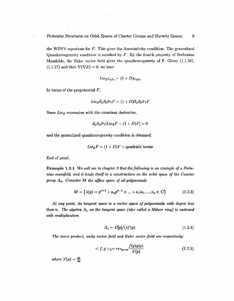
Example 1.2.1 We will see in chapter 3 that the following is an example of a Frobe
nius manifold, and it lends itself to a construction on the orbit space of the Coxeter
group An. Consider M the affine space of all polynomials
M = (A(p) = pn+1 + anpn~x + ... + oi|oi,...,an e C) (1.2.3)
At any point, its tangent space is a vector space of polynomials with degree less
than n. The algebra A\ on the tangent space (also called a Milnor ring) is endowed
with multiplication
Ax=C\p]/(\)'(p) (1.2.4)
The inner product, unity vector field and Euler vector field are respectively:
<f,9>x=res^&ffi (1.2.5)
where X'(p) — ^

Frobenius Structures on Orbit Spaces of Coxeter Groups and Hurwitz Spaces 10
e = d
day
E = -^Y>~i + l^a re + 1 ddi
(1.2.6)
(1.2.7)

Frobenius Structures on Orbit Spaces of Coxeter Groups and Hurwitz Spaces 11
1.3 Physical Normalization and Polynomial Solu
tions to WDVV
We now introduce the normalization for the prepotential F prescribed by the
physical literature.
Lemma 1 The scaling transformations generated by the Euler vector field E (1.1.8)
act by linear conformal transformations of the metric r)ap
LieEr}a0 = (dF - d^rj^ (1.3.1)
Proof. Differentiating (1.1.8) wrt t1, ta and tfi and recalling Liepd\ = —didi, we
obtain the Lie derivative of the metric. End of Proof.
Corollary 1 lfr]u=0 and all the roots of E(t) are simple then by a linear change
of coordinates ta the matrix nap can be reduced to the antidiagonal form
Va/3 — <W,n+l
In these coordinates F(t) has the following form for some function f(t2,... ,tn)
1 1 n - l
F(t) = ^(t1)2^ + ^t1 ^ tatn~a+1 + f(t2, ...,tn) (1.3.2)
The sum
2V ' 2 a=2
da + «n_Q+l
does not depend on a and
dp = 2d% + dn.
When the degrees are normalized so that di = l, they have the form
da = 1 — qa dp = 3 — d
for numbers qi,..., qn, dn, d given by
Qi = 0, qn = d, qa + g„_Q+i = d
Proof. If (ei,ei) = 0 then vector en may still be chosen to be an eigenvector of
the scaling transformations of the Euler vector field (i.e. roots of E(t)). Using only

Erobenius Structures on Orbit Spaces of Coxeter Groups and Hurwitz Spaces 12
such eigenvectors on the orthogonal complement of the span of e\ and en, r}ap can
be reduced to the antidiagonal form. Recalling t)ap := CiQ/9, the antidiagonal form in
these coordinates determines the above form of the prepotential F. Independence of
the sum da + d„_a+i and dp — 2d\ + dn follow directly from the action of the scaling
transformations on the metric, (1.3.1). End of proof.
Example 1.3.1 Let us look at the n = 3 case in the algebra At with basis e\ — 1, e2,
e3 and prepotential function F for some function f(x, y)
F(t) = \t\h + \txt% + f(t2, t3) (1.3.3)
The multiplication table (with subscripts of f as partial derivatives) is given by
^2 Jxxy^l ' Jxxx*'2 ~>
^2^3 = fxyyCl + fxxy^2
e 3 ~ / w y e l ' Jxyy&2
The associativity condition
(el)e3 = e2(e2e3)
gives the following partial differential equation for f(x, y)
Jxxy = Jyyy < Jxxxjxyy
Note that (1.3.5) is the only associativity equation for n — 3, i.e.,
(ei)e2 = e3(e3e2)
gives nothing new.
Dubrovin has conjectured that any solution of W D W with good analytic proper
ties has a discrete group for its monodromy group, as we shall investigate in chapter
3. Starting this way, Probenius manifolds are constructed on the orbit spaces of Cox
eter groups, generating a class of solutions that are polynomial in nature. Let us now
describe these with examples from dimension n = 3.
Polynomial Solutions of WDVV
Consider Probenius Manifolds whose structure constants are all analytic at the point
(1.3.4)
(1.3.5)
(1.3.6)

Frobenius Structures on Orbit Spaces of Coxeter Groups and Hurwitz Spaces 13
t = 0. The Frobenius algebra A0 := Tt=oM has at point t = 0 structure constants
c^g(0) and basis vectors e j , . . . , e„. The ga as denned in Corrolory (1) give the degrees
of the basis vectors as
degea = qa
The germ of the Frobenius Manifold near t = 0 is a deformation of the algebra A0,
and thus the algebras At for ^ 0 are deformations of Ao. This analytic deformation
is physically relevant as we shall see in chapter 2. The algebra Ao corresponds to the
primary chiral algebra of a topological conformal field theory; an operator algebra of
the perturbed topological field theory. If in the normalization of (1.3.2) we constrain
that the degrees degta be positive real numbers, then 0 < d < 1. Paired with the
quasihomogeneity condition (1.1.6), this amounts to finding the polynomial solutions
F(t) of the WDVV equations.
Example 1.3.2 We consider the case of dimension n = 3. The prepotential is, as
before (1.3.3)
F(t) = 1^3 + ^4 +f(t2,t3)
The degrees as prescribed by the normalization are:
degt1 = 1 (1.3.7)
degt2 = 1 - g
degt3 = l-d
degf — 3 — d
The function
f(x,y) = ^2apgafyq
must satisfy the quasihomogeneity condition, i.e.
P Qpg^O when p-\-q — 3= ( - + ? — l)d k2
Now the function f has two possible forms.
1) For n odd: n,m£ N,
f = Y afe*4-2*"1/"-1 d - ^ - ^ n — m

Frobenius Structures on Orbit Spaces of Coxeter Groups and Hurwitz Spaces 14
2) For m odd: n,m € N,
2(n — m) f = Y, afcX4-*"*!/*"-1 d =
2n — m
The powers in f must be nonnegative. and cases for which f is a cubic or lower
are uninteresting. This leaves three possibilities:
a) f = a x V " 1 + by2n~\ n>3 (1.3.8)
b) f = ay"-\ n > 5
c) / = a x V " 1 + bxY"'1 + cxy3"'1 + dy4n~\ n > 2
As in the example preceding, f must satisfy the partial differential equation (1.3.6)
from which we may solve for n. In (1.3.6) f with form a) deems n — 3; with form b)
there is no solution; with form c) deems n — 2 or n — 3. We thus have as the three
remaining polynomial solutions for WDVV with positive degrees of ta in dimension 3:
txt3 + tjt2 ig*3 , h (-, o n\ F~ 2 + ^ + 60 ( L 3 - 9 )
Fss^ + tA + ^ + M + ± (1.3.10)
^ ^ T M + f + f + 4 (L3-H)
The prepotential (1.3.9) has the same form as in Example 1 with n — 3, that we will
see in chapter 3 may be constructed on the orbit space of the Coxeter group An. In
the same vein, polynomials (1.3.10) and (1.3.11) are related to the Coxeter groups
Bn and Hn respectively.
Chapter 2
Topological Field Theories
Here we describe topological field theories as background independent quantum
field theories, describe the matter sector of such theories, and give Atiyah's axioms
[1],[7],[10], [11]. We then show that the matter sector for a 2D-topoIogical field theory
is always encoded by a Frobenius algebra[l],[7],[9]. The moduli space generated by
topological conformal field theories is a Frobenius manifold, and we give the example
of Topological Landau-Ginzburg models, which we will see in chapter 3 corresponds
to the Frobenius manifold of Example (1.1) [7],[10].
2.1 2D-Topological Field Theories and Atiyah's Ax
ioms
A quantum field field theory (QFT) in its Lagrangian formulation may be specified
on a D-dimensional manifold E as:
1) A family of local fields <pa(%), x € S. These may be functions or sections of a
fiber bundle over E. A metric 9ij{x) is usually one of the fields (the gravity field).
2) A Lagrangian L — L(<p, <px---) and classically, the Euler Lagrange equations:
6S 0 (2.1.1) 6ifa(x)
S[<p]= [L(ip,yx...)dZ (2.1.2)
3) A Quantization procedure via the path integral approach where a path inte
gration measure [d<p] is constructed (but almost never well-defined) and the partition
15

Frobenius Structures on Orbit Spaces of Coxeter Groups and Hurwitz Spaces 16
function Z s results from path integration over the space of all fields <p(x).
Zx = J[dV>]e~SM (2-1-3)
Correlation functions (The output of a QFT: its physical observables) are defined
similarly:
Here the definition of a QFT involves a choice of a manifold E on which the
QFT lives and a choice of metric, a background field. Thus, the correlation functions
are calculated in a certain background. We now consider a class of 2D-QFTs: 2D-
topological field theories (TFT). These are background independent QFTs; those
whose correlation functions do not depend upon the choice of metric. TFTs are
invariant wrt arbitrary changes of the metric g%j{x) on a 2D surface E:
5gij(x) — arbitrary, 5S — 0
As a step towards a rigorous account of TFTs, Atiyah formulated axioms describing
them for arbitrary dimension. These axioms describe correlators of fields in the mat
ter sector of a 2D-TFT. In this sector, the local fields <fi(x),..., <pn{x) do not contain
a metric on the surface E. Atiyah found that in the matter sector, the correlators
of the fields obey three simple axioms. Here we describe the matter sector and give
Atiyah's axioms for dimension D = 2.
Matter Sector for a 2D-TFT:
1) A: the space of local physical states. We assume A is finite-dimensional.
dimA — n < oo
2) The assignment T
T : (E, dT.) —> v{sm e A{S>ds) (2.1.5)
which only depends on the topology of the pair (E, dH) for E an oriented 2-surface,
and dE its oriented boundary. We are assigning to each local physical state Vi an

Frobenius Structures on Orbit Spaces of Coxeter Groups and Hurwitz Spaces 17
oriented 2-surface with oriented boundary. (Note that when the surface is closed, it's
boundary is null.) The linear space A^,dT.) is:
f C if d£ = 0 As,0E) = { (2.1.6)
j Ai <g>... <g> Ak if dT, consists of k oriented cycles C\... Ck
_ J A if C, is ori
* ~ \ .4* (dual) oth
oriented with E . \£> J- - I J
otherwise
Atiyah's Axioms for a 2D-TFT:
The 2D-TFT T satisfies 3 axioms. (Only the orientation of the boundary dT, is shown.
A cycle Ci will be oriented with the surface S if S remains to the left traversing in
the direction of Ci. Assume the surfaces are oriented wrt the external normal vector.)
1) Normalization:
Figure 2.1: Normalization
2) Multiplicativity: If
(S,0E) = (E^dEi) U (E2,0E2) (2.1.8)
then
«(S,0E) = f(Si,0Ei) ® W(s2,as2) ^ ^4(s,9S) (2.1.9)
and
A(Stas) = AEi,a£i) ® ^(S2,9E2) (2.1.10)
3) Factorization: T h e ope ra t ion of cont rac t ion for tensor p roduc t s :
Ax <g>... <g> ylfe -»• Ax <g>... <g> At <g> . . . <g> A,- <g> . . . <8> j4fc (2.1.11)

Frobenius Structures on Orbit Spaces of Coxeter Groups and Hurwitz Spaces 18
is defined when Ai and Aj (the hats denote their omission) are dual to each other
and identity on the other factors. Pictorially, we see that if (E, dH) and (£', dT!) are
identical outside of a ball and inside are as in figure 2.2, then
Figure 2.2: Factorization
^(E,as) = iojo contraction of U(S',ai:') (2.1.12)
is obtained by gluing together the cycles C^ and CJ0.
Now we present a symmetric polylinear function v9tS on the space of states A; the
genus g correlators of the fields </?ai,..., <pat For example:
And in some basis <pi,...,y„in A:
VgAfm ® - - • <8> <Pa„) =•• (<Pai • • • <Pa»)g (2.1.13)
Figure 2.3: Here g — 2 and s — 3

Frobenius Structures on Orbit Spaces of Coxeter Groups and Hurwitz Spaces 19
2.2 2D-Topological Field Theories and Frobenius
Algebras
Now we come to the main theorem of the chapter. The space of states A (the
matter sector of a 2D-TFT) carries a natural structure of a Frobenius algebra, and
all the genus g correlators of the fields can be expressed very simply in terms of this
algebra [7].
Theorem 2 Let (I) The tensors c, rj, on A form a Frobenius algebra structure with
\ J / e A*«>A*<8>A = HOM(A®A,A)
Figure 2.4: Multiplication
Figure 2.5: Inner Product
unity e defined as in figure 2.6.

Frobenius Structures on Orbit Spaces of Coxeter Groups and Hurwitz Spaces 20
(D e = * € A
Figure 2.6: Unity
(II) Let the Handle operator H be defined as in figure 2.7.
H= v: v t eA
Figure 2.7: Handle operator
Then, the genus g correlators may be expressed as the following R.H.S. product in
the algebra.
(<Pai •••tPak}g=(<Pai*---* Vak, Hg) (2.2.1)
Proof:
(/) The algebra must be commutative. Looking at figure 2.4, the multiplication
c is seen to be commutative since we may always exchange pant legs by a homeo-
morphism. Similarly, by figure 2.5 the inner product rj is seen to be symmetric by
a homeomorphism. The multiplication must also be associative, and this is demon
strated in figure 2.8:

Frobenius Structures on Orbit Spaces of Coxeter Groups and Hurwitz Spaces 21
Figure 2.8: Associativity
The more general k-product is realised by the k-leg pants in figure 2.9:
U eHOM(A®k ,A)
Figure 2.9: k-product

Frobenius Structures on Orbit Spaces of Coxeter Groups and Hurwitz Spaces 22
The Identity:
Figure 2.10: Identity
The inner product rj must be nondegenerate, so we find its inverse. Let
r\ e A*® A
Figure 2.11: Inverse

Frobenius Structures on Orbit Spaces of Coxeter Groups and Hurwitz Spaces 23
Then, fjrj is easily seen to give the identity cobordism, so fj — n .
id
Figure 2.12: Nondegeneracy
The multiplication c (figure 2.4) must be compatible with the inner product 77
(figure 2.5) as indicated by the following:
Figure 2.13: Invariance

Frobenius Structures on Orbit Spaces of Coxeter Groups and Hurwitz Spaces 24
(i7) For any vg>s, we may construct these correlation functions using members of
the algebra. For example, using the multiplication c, the inner product r\, the 3-leg
product and 3 handle operators Hg, we have:
Figure 2.14: Correlation functions
End proof.
For a TFT T (2.1.5) and unity e (figure 2.6), the image of e under T gives the
vector space A := T(e). The image of the co-unity 8 (e with reversed boundary
orientation) under T gives the dual space A* :— T(0) Note that the pairing rj and
unity e may be used to define 9:
•CD-Figure 2.15: Co-unity 0

Frobenius Structures on Orbit Spaces of Coxeter Groups and Hurwitz Spaces 25
The nondegeneracy of n given the co-pairing rj'1 as seen in figure 2.14. yields an
isomorphism between A and A* - the identity cobordism as seen in figure 12. This is
the content of Atiyah's axiom [1] dT, H-> A => dT, •-» A*.
The boundary dT of E (if dT ^ 0) consists of oriented cycles C*. Ci will correspond
to A if oriented with E, and will correspond to A* if oriented against E. The gluing
along a cycle Ct (the disjoint union of {Tj,dTi) and (E2,<?E2)) corresponds to the
tensor product contractions of dual vectors. We now see several examples of this [11],
using the notations from chapter 1:
Example 2.2.1 c ^ : A ® A -* A e A* <g> A* <g> A, a (2, l)-tensor ea®ep = c^e^
:Ci : = trc
Figure 2.16: Multiplication c
Example 2.2.2 e : C—>• J4 G A, vectors
Figure 2.17: Unity e

Frobenius Structures on Orbit Spaces of Coxeter Groups and Hurwitz Spaces 26
Example 2.2.3 9 : A -> CeA*, co-vectors
9 :
Figure 2.18: Co-Unity 9
Example 2.2.4 JJ : A <g> A -> C € A* <8> A*, a (2,0)-tensor r\lt =< e^,e6>
*k := C i«y
Figure 2.19: Pairing rj
Frobenius Structures on Orbit Spaces of Coxeter Groups and Hurwitz Spaces 27
Example 2.2.5 rfl : C-> A ® A € A <g> A, a (0,2)-tensor rpl =< e7,e£ >
I f : : if: = (V1
Figure 2.20: Co-pairing •q l
Example 2.2.6 id : A -> A € A* ® A
id =
Figure 2.21: Identity
Frobenius Structures on Orbit Spaces of Coxeter Groups and Hurwitz Spaces 28
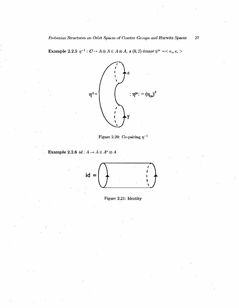
Example 2.2.7 cea0 : A <g> A ® A E A* <gi A* <g> A*, a (3,0)-tensor ceaB = JH^.0%
'. V ^ E < $
Figure 2.22: 3-point function
Example 2.2.8 Using the co-pairing rfe and 3-point function ctap, we can recover
the multiplication c by gluing along e; contracting e
: T T C .
Figure 2.23: clp = rptcta0
Frobenius Structures on Orbit Spaces of Coxeter Groups and Hurwitz Spaces 29
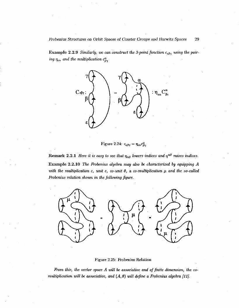
Example 2.2.9 Similarly, we can construct the 3-point function ct/g7 using the pair
ing rjCQ and the multiplication djL
c* *1 C! •sec p'f
Figure 2.24: c£/j7 = i]iacf^
Remark 2.2.1 Here it is easy to see that nap lowers indices and rfP raises indices.
Example 2.2.10 The Frobenius algebra may also be characterized by equipping A
with the multiplication c, unit e, co-unit 6, a co-multiplication /z and the so-called
Frobenius relation shown in the following figure.
Figure 2.25: Frobenius Relation
From this, the vector space A will be associative and of finite dimension, the co-
multiplication will be associative, and (A, 6) will define a Frobenius algebra f 11].

Frobenius Structures on Orbit Spaces of Coxeter Groups and Hurwitz Spaces 30
2.3 Topological Conformal Field Theories and Topo
logical Landau-Ginzburg Models
Theorem 2 says that the matter sector of 2D-TFT is always encoded by a Frobe-
nius algebra. The Frobenius algebra on the space of states A is called the primary
chiral algebra of the TFT. To preserve as much information as possible in generating
the correlators from the Lagrangian, not only the Lagrangian but also its topologically
invariant deformations are considered:
L-^L + ^eL^
where ta are coupling constants. We now have a moduli space of TFTs. A large,
physically relevant class of such moduli spaces of TFTs are topological conformal field
theories (TCFT). There is a physical theorem which asserts the canonical moduli
space of a TCFT carries the structure of a Frobenius Manifold [7]. Examples of
TCFT include the Topological A-models (Kahler moduli) and Topological B-models
(complex moduli) famously related by mirror symmetry and ones we consider next:
Topological Landau Ginzburg models (polynomial moduli, which are included in the
family of topological B-models).
Example 2.3.1 Topological Landau-Ginzburg (LG) Models:
The Bosonic part of the LG action is:
' - ! * *
dp 2
dz + |A'(P)|2) (2.3.1)
where X(p) is a holomorphic function called the superpotential, and S is a functional
of the holomorphic p(z) called the superfield. The Classical states correspond to the
critical points of \(p), where
Pi := p(z) for \'(pi) — 0,i — l...n
A family of LG models (the moduli space of the LG-theory) is obtained by deforming
the superpotential
\ = \(P;t1,. ..,*")
for parameters t = (t1,... , t n ) , and the Frobenius structure on the space of parameters

Frobenius Structures on Orbit Spaces of Coxeter Groups and Hurwitz Spaces 31
is given by:
(S, P. ff\ = £ ^ y M (2-3-3) A'=0 W' P
where the vector fields d, &, d" on the space of parameters are taken keeping p constant.
For the particular superpotential
its deformed superpotential matches the polynomial of Example (1.1). We will see
this in chapter 3.
Chapter 3
Unfoldings of Singularities and the
Orbit Space of a Coxeter Group
We will describe the unfoldings of singularities of An type in section one and verify
its Probenius structure [2],[14]. In section two we describe the FVobenius structure on
the space of orbits of a Coxeter group [4],[7], and in the third section we verify that
the structures from Examples (1.1) and (2.1) are FVobenius, and coincide with the
FVobenius structure on the orbit space of Coxeter group An [7], [17].
3.1 Unfoldings of Singularities
Using unfoldings, one may construct a product and flat metric on the space of
parameters M = C n and establish canonical coordinates that determine the Euler
vector field [2],[14]. In this section we will see how our main example of Ai-type
exhibits a natural FVobenius Manifold structure in the unfoldings of singularities.
The unfolding F^ of the polynomial f(z) = zn+1 gives the space of parameters a rich
structure. Consider only germs, so M = Cn . By choosing a basis for the vector
space Qp( (the Jacobian algebra), the tangent space T^C" is given the structure of a
commutative algebra with unit. Here the product at a point £ G C" is denoted by
*£, and the £o-axis gives the identity vector field £- in all Tf C". A theorem by K.
Saito states there is an isomorphism of vector bundles over Cn , so that at any point
f the isomorphism Qp^ —»• T£Cn transports the bilinear form 0 to a flat metric on C n
[14]. Let us consider the unfolding i^, flat metric and bilinear form 6 in our main
example.
Example 3.1.1 A„-type unfolding: Let us consider the polynomial f(z) = zn+1 and
32

Frobenius Structures on Orbit Spaces of Coxeter Groups and Hurwitz Spaces 33
its unfolding Fi=zn+l+^_lZn-l+^+^ £€Cr) (3.1.1)
Its space of parameters is the affine space of all polynomials F^. At any point, the
tangent space is the vector space of polynomials with degree < n — 1. The product
a *£ @ at this point of Qp = C[z]/ < F, > is the remainder of a/? in the Euclidean
division by F^.
The one-form d is 1 f adz „ adz .„ , „.
a"Wrip-'to»ir (312)
To see that it defines a flat metric, we look for the flat coordinates in which 6 is
constant. To do this we invert and solve the equation
w Ji+1 F,{z)
w = z + 0(z'1)
expanding the solution for z large, so that
= w+tJtzl + ^, + ^ + o(^-] (3.1.3)
w wn \wn+1J
where to • • • t„_i is a basis of the vector space of symmetric polynomials. Then to • •. <n_i
are seen to be the flat coordinates by,
and using
we have
^(FJ = ^(z(w,t))^- = F'^z{w,t)w-n+i (3.1.4)
Fi(z)dz = (n + l)wndw (3.1.5)
<?( J ^ ) , £;&)) = -Resz=O0F^z{w,t))W-2n^dz (3.1.6)
= - ( n + l)Resw=00w-"+i+jdw (3.1.7)
= (n + l)6Hjjn_i (3.1.8)
(3.1.9)
the metric flat and nondegenerate everywhere.
Now we would like to establish the canonical coordinates and the Euler vector field.

Frobenius Structures on Orbit Spaces of Coxeter Groups and Hurwitz Spaces 34
The canonical coordinates are chosen to be the critical values of F^ : x,- = F^qi). The
vector fields forming a basis for the algebra QFK are then ^ . For any polynomial P 6
C[z\,... ,Zk] with m critical points, the vector field is written in canonical coordinates
as:
The unity vector field is: 771 r\
1 = 1 o x l
The unfolding F^ itself is now an Euler vector field
^ = E^%r = E ^ - : i ; < 3 1 1 2 > since it rescales the product *̂ according to (1.1.17). Lastly, we check the Euler
vector field E acts by conformal transformations of the metric and that V(V-E) = 0.
Looking at the Euclidean division of F^ by Ft, we may write the Euler vector field E
in coordinates (£o, • • • -. fn-i) as
In flat coordinates, and recalling from (3.1.3)
U = - & + Bi(Cm, • • -, &.-i) 0 < i < n - 1
we assume deg(£j) = n — j + 1 so that deg(F^(z)) = n + 1, deg(Bi) = n — i + 1 and
botk F{ and Bt are homogeneous. Then,
rc+1 v n + 1 A" n+1 Jd£,-
" ^ „U6,
Frobenius Structures on Orbit Spaces of Coxeter Groups and Hurwitz Spaces 35
by the homogeneity of Bi7 so that in flat coordinates,
Any space of parameters of a versal unfolding is isomorphic to the space of orbits
of a Coxeter group, and we will see their Frobenius structure in the next section.
Also Dubrovin conjectured that all polynomial solutions of the WDVV equations are
potentials of these structures. This was later proved by Hertling [8].
Frobenius Structures on Orbit Spaces of Coxeter Groups and Hurwitz Spaces 36
3.2 Frobenius Structure on the Orbit Space of a
Coxeter Group
In this section, we first define the intersection form, flat pencil of metrics and
the monodromy group of a Frobenius manifold [4],[7]. We then show the Frobenius
structure on the orbit space of a Coxeter group. These manifolds are polynomial in
nature and each possesses a finite Coxeter group as its monodromy group [7].
Given a Frobenius manifold M we may use the invariant inner product n (1.1.2),
to define another flat metric (, )* called the intersection form.
Definition 3.2.1 The intersection form is given by
{x,y)*:=iB(x*y) (3.2.1)
for x,y ET*M and ij$ the inner derivative of a Inform with the Euler vector field E.
The components of (, )* in flat coordinates ta are:
gap:={dta,dt0)* = Ee(t)^{t) (3.2.2)
where
dy.(t):=rr<£M (3-2-3)
Here n has been used to extend the multiplication and Frobenius structure from the
tangent bundle to the cotangent bundle. Having established these metrics as fiat,
Dubrovin proved further that any linear combination of them is also flat, defining the
flat pencil of metrics. Consider two non-proportional metrics (,)j and (,)£ and their
corresponding Levi-Civita connections V\ and V£.
Definition 3.2.2 Two metrics form a flat pencil if:
1) The following metric is flat for A arbitrary
j^gV+Xg? (3.2.4)
2) The Levi-Civita connection for this metric has the form
r* = rrfc + Aii (3.2.5)

Frobenius Structures on Orbit Spaces of Coxeter Groups and Hurwitz Spaces 37
Consider the metrics (. )* and (, }* on the Frobenius Manifold M, where (, )* is induced
on T*M by 77 = (.) and the Euler vector field E is linear in the flat coordinates.
Proposition 3.2.1 The metrics (,)* and (,)* form a flat pencil on M.
Remark 3.2.1 On M. the difference tensor is defined by:
Aijk = 9isriks-g?rik
s (3.2.6)
Dubrovin's geometry of flat pencils of metrics [7], gives the following proposition:
Proposit ion 3.2.2 For a flat pencil of metrics a vector field f = /'#,- exists such
that the difference tensor (3.2.6) and the metric g1? have the form
Aijk = V|V£/fc (3.2.7)
gl^Vif + Vif + cg? (3.2.8)
for some constant c. The vector field satisfies the equations
AiJAf = AfA? (3.2.9)
where
A? := fttt.A-« = V 2 f e V ^ (3.2.10)
(gTd1 - 9\s9?)V2sV2ifk = 0 (3.2.11)
Conversely, for a flat metric gl% and solution f of (3.2.9),(3.2.11) the metrics g^ and
g%2 form a flat pencil.
Later in this section, we will see that from the intersection form, Euler vector field
and unity vector field, one can uniquely reconstruct the Frobenius structure. We now
describe the monodromy grpup of a Frobenius Manifold.. The intersection form or
contravariant metric (, )* is degenerate on the discriminat locus S where the discrim
inant A(t) vanishes:
A(t) := det(gafi(t)) = 0 (3.2.12)
S c M where
S := {tA{t) := det{ga0(t)) = 0} (3.2.13)
Since (, )* and 17 are defined outside of the discriminant locus E, a Frobenius manifold
defined by {M/T., (, )*) is not simply connected. Thus at any point there will be a

Frobenius Structures on Orbit Spaces of Coxeter Groups and Hurwitz Spaces 38
nontrivial holonomy group at any point, being a discrete subgroup of 0(n, C) [4]. An
isometry $ can be specified of a domain Q in n-dimensional complex Euclidean space
En to the universal cover of M/E:
$ : f t ^ M / E (3.2.14)
Then the action of the fundamental group 7ri(M/E) on the universal cover is lifted
to an action by the isometries of En. This isometry (3.2.14) is contructed by fixing
a point po G M outside of E and expressing y = (y1,... ,yn) the flat coordinates
of (,)* in terms of the flat coordinates t = (t1,.••>*") of n. Germs of functions
y'it1,... ,tn) will be multivalued around E, and the set of non-contractible loops 7
around E correspond to linear affine transformations of the y"s. In this way, the map
and group homomorphism fx is obtained:
H:ir1(M/Y,)-+Isometries(En) (3.2.15)
Definition 3.2.3 The image of the fundamental group under [i defines the mon-
odromy group W(M) of the Frobenius Manifold:
W(M) := /i(wi(M/E)) C IsometriesiE") (3.2.16)
Remark 3.2.2 The flat coordiantes y = (y1,... ,yn) are found by solving the follow
ing system, where V denotes the Levi-Civita connection for the intersection form (the
Gauss-Manin connection):
VaV0-=9ae(t)dadpy + T£(t)dty = O (3.2.17)
for a , / ?= l,...,n
Inversely, we next describe the construction of polynomial Frobenius manifolds
whose monodromy group is a Coxeter group preserving invariant the intersection
form (,)*. Let W be a finite Coxeter group; a finite group of linear transformations
of an n-dimensional Euclidean space V generated by reflections [5]. The orbit space
M — V/W has the structure of an affine variety, where the coordinate ring of M is
identified with the coordinate ring of VK-invariant polynomials over V. The coordinate
ring of M has as a basis invariant homogeneous polynomials y%. Their degrees a\ are
invariants of the group W. The maximal degree h is called the Coxeter number of
Frobenius Structures on Orbit Spaces of Coxeter Groups and Hurwitz Spaces 39
W. di := degtf) (3.2.18)
d-i = h > d2 > . . . > dn-i >dn = 2 (3.2.19)
For example, group An has degrees di = n + 2 - i and group Bn has degrees di =
2(n - i + 1). The action of W is extended to the complexified space
M = V ® C/W
Coordinates on V will be denoted by a;".The Euler vector field is:
E - - ( d l 2 M + . . . + dnyndn) = -xa— (3.2.20)
The invariant coordinates will be denoted as yn and normalized as:
y n = ^ ( ( * 1 ) 2 ) + --- + ( x n ) 2 ) ) ( 3 - 2 ' 2 1 )
where (.,.) denotes the W-invariant Euclidean metric on V, and is extended onto M
as a complex quadratic form. We denote here by (., .)* the contravariant metric on
the cotangent bundle T*M induced by the WMnvariant Euclidean metric on V.
Lemma 2 The Euclidean metric of V induces a polynomial contravariant metric (,
) * (the intersection form) on the space of orbits
^ (V) = ( * W ) * := | £ ^ (3-2.22)
and the corresponding polynomial contravariant Levi-Civita connection (the Gauss-
Manin connection)
Remark 3.2.3 The intersection form (3.2.22) and Gauss-Manin connection (3.2.23)
are graded homogeneous polynomials that depend linearly on y1, with degrees:
deggii{y) = di + dj-2 (3.2.24)
deg rij(y) ^di + dj-dk-2 (3.2.25)
Theorem 3 There exists a unique, up to an equivalence, Frobenius Structure on the
space of orbits of a finite Coxeter group with the intersection form (3.2.22), the Euler

Frobenius Structures on Orbit Spaces of Coxeter Groups and Hurwitz Spaces 40
vector field (3.2.20) and the unity vector field e := TA-
To prove this main theorem, we give the Saito metric (3.2.26) in lemma 3, Saito
flat coordinates ^(x),...,tn(x) in lemma 4, and the associated components of the
intersection form and Gauss-Manin connection in lemma 5. Then the existence of the
Frobenius structure on the orbit space of a Coxeter group is proven in lemma 6 with
uniqueness following.
Lemma 3 The triangular matrix
r)ij(y)-=d1gij(y) = Ofori + j>n + l (3.2.26)
has constant nonzero antidiagonal elements
d := ^n-i+1), (3.2.27)
and
c := det{rfj) = ( - l ) 2 ^ ^ , . . . , c + 0 (3.2.28)
Lemma 4 There exist homogeneous polynomials tx{x),... ,tn(x) of respective degrees
di,...,dn such that the matrix
if* :=di{dta,dt0)* (3.2.29)
is constant
Lemma 5 For coordinate tn normalized as in (3.2.21), we have the following (with
no summation over repeated indices):
g™ = !kt« (3.2.30) n
TT^dau 6P (3.2.31) fh
Lemma 6 Let t1,..., t" be the Saito flat coordinates on the space of orbits of a finite
Coxeter group and
rf" = diidP^dtPy (3.2.32)
be the corresponding constant Saito metric. Then there exists a quasihomogeneous
polynomial F(t) of degreee 2h+2 such that
(dta, dt?y = {da + dlf~
2\aXrf'idxdtlF{t) (3.2.33)

Frobenius Structures on Orbit Spaces of Coxeter Groups and Hurwitz Spaces 41
The polynomial F(t) determines on the space of orbits a polynomial Frobenius struc
ture with the structure constants
ca/jW = r,^dadpdtF{t) (3.2.34)
the unity
e = dx (3.2.35)
the Euler vector field
E = Y(1 - ^-)tadQ (3.2.36) A—1 h
and the invariant inner product r\.
Proof. Using lemma 4 and proposition 3.2, we represent for some vector field f^(t)
the tensor Tf(t) as
Tf(t) = r)aidr,d1f(t) (3.2.37).
Also, T"P(t) must satisfy the conditions
s/aarp = gP*TY' (3.2.38)
For a = n, lemma 4 and the Euler identity it follows that
(d, - 1)<A = ] T rf<{dy - de + h)dtP = (dy + dfi - 2)rfldtP (3.2.39)
which gives the symmetry condition (3.2.41) by defining
jn fr
h dj — 1 (3.2.40)
rf€dtFi = rf'dtF13 (3.2.41)
Hence there exists a quasihomogeneous polynomial function F{t) in t1,..., tn with
degree 2h + 2 such that
Fa = naedtF (3.2.42)
Equation (3.2.33) follows from (3.2.41) and (3.2.39), and writing
cf{t) = rfxrf>idxdlid^F (3.2.43)

FYobenius Structures on Orbit Spaces of Coxeter Groups and Hurwitz Spaces 42
•7
ra/3
=
cT
4°
h °1
~ °7 C(T
— Aa ~°0
we have the following:
(3.2.44)
(3.2.45)
(3.2.46)
End Proof.
This structure is unique. For a polynomial Frobenius structure on M with Euler
vector field (3.2.20) and Saito invariant metric, F(t) must satisfy (3.2.33) up to a
quadratic polynomial. We consider in the Saito flat coordinates
dta • dtp = r}aXr}^dxdtld^F(t)dt'1 (3.2.47)
and by the definition of the intersection form we have
iE{dta,dtP) = I Y , d^r,aXV^dxd^F(t) (3.2.48) 7
= \{da + dp- 2)r}aXrf»dxdllF{t) = {dta, dtP)* (3.2.49)
Frobenius Structures on Orbit Spaces of Coxeter Groups and Hurwitz Spaces 43
3.3 Example of Frobenius Structure on the Orbit
Space of Coxeter Group An
The group W = A„ acts on R"+ 1 = (£0,£1, • - •, £n) by permutations
(Co, 6 > • • • .£»») *-* (£<T(0),£<T(1), • • - , & ( « ) )
restricted to the hyperplane
£ o + 6 + - - + £n = 0 (3.3.1)
The invariant metric is the Euclidean metric on (3.3.1), and the invariant polyno
mials are the symmetric polynomials. A homogeneous basis in this ring of invariant
polynomials is given by the elementary symmetric polynomials:
a* = (-l)"- fe+1te>6--6fc-- • + •••), * = l , . . . , n (3-3.2)
The complexified space of orbits M — Cn/An is then identified with the space of
polynomials \(p) from example (1.1). We now show that the Frobenius structure on
M from lemma 6 coincides with the structures of examples (1.1) and (2.1) [7], [17].
Theorem 4 1. For example (1.1), the inner product (,) and tensor c(.,.,.) =
(. * ., .)A have the form
<* »•>, ~ £ fe^./(AWX)(A(PW (3-3,3)
*—' dpdXyp)
2. Let q1,..., qn be the critical points of the polynomial \(p),
X'(qi) = 0, i = l,...,n
and
u* = A(fl*), i = l,...,n (3.3.5)
be the critical values. Here u1,..., un are local coordinates on M near A where
X(p) has only simple roots. These local coordinates are the canonical coordinates
for multiplication of example (1.1) and in these canonical coordinates the metric

Frobenius Structures on Orbit Spaces of Coxeter Groups and Hurwitz Spaces 44
from example (1-1) has the diagonal form
<,>U=^%(«)(rft i<)2 , **(*) = j ^ (3-3-6)
d'. d". &" are any tangent vectors on M in a point X, where derivatives are taken
keeping p constant. X'(p) and X"(p) are the first and second derivatives wrt p.
3. The metric on M induced by the invariant Euclidean metric at a point X for
which X(p) has simple roots may be written as
{cy,tvh = _ E ^ e S d A = o ^ ^ A ( p ^ ^ A ( ^ ) ( 3 3 ? )
Proof. 1. Equation (3.3.3) corresponds to the invariant inner product from exam
ple (1.1):
l f n \ P o o f(P)sJP)
(f,9)x = Resp=00
By letting cr" — f, & — g and X'(p) = —^- and denoting by tv the meromorphic
differential: , , &{x{p)dp)ty'{x{p)dp) u=—2W)— ( 8)
we apply residue theorem on to. The inner products are seen to correspond to each
other since the sum of residues of a meromorphic differential on the Riemann p-sphere
is zero. Restock) + ]jr Res\x\<00u = 0 (3.3.9)
Equation (3.3.4) corresponds to the multiplication from example 1.1. Using equation
(3.3.9) and letting f(p) = &{X{p)), g(p) = d"(X(p)), and h(p) = &"{X{p)) to re-write
dpdXyp)
For polynomials q{p) and r(p) where deg(q) < n, f(p)g(p) = q(p) + r(p)X'(p), and in
the Milnor ring C\p]/(X'(p)), we will have the multiplication f*g — qso that
(3.3.11)
Since the second residue vanishes, the first residue is the inner product:
(q, h)x = (f*g, h)x = c(f, g, h) (3.3.12)

Frobenius Structures on Orbit Spaces of Coxeter Groups and Hurwitz Spaces 45
2. The intersection form in the hyperplane coordinates has the form:
ab = 5ab L_ (3.3.13) y n + 1 ;
Denote the roots of A'(p) by q\
Ui = KQi) * = ! , - • • ,« (3.3.14)
9iA(p)|p=gj = di,- (3.3.15)
Using (3.3.14),(3.3.15) and the Lagrange interpolation formula, we get
Since X(p) and A'(p) are given by
n
o=l
it follows that
(^6 =...+$e») na> - 6) - X) - ^ r ^ ° = d*w (3-3-17) 6=1 a = l P k*
Substituting p = £„ in the previous equation, we get
^'"(c-^W)' ''a = 1'-'n (3318)
Prom (3.3.3), (3.3.4), and (3.3.15) we obtain
(ft-,ai) = - * i ^ j j (3.3.19)
C(di, dU di) = (ft * di, di) = - j^-rr (3.3.20)

Frobenius Structures on Orbit Spaces of Coxeter Groups and Hurwitz Spaces 46
Now we see that u1... un are the canonical coordinates, since in the algebra we have
dt * dj = 8^ (3.3.21)
3.From (3.3.4) and (3.3.15), we have
i f c ( „ ) : = ( a , a ) - = _ _ ! _ (3.3.22)
Using this, we obtain
n £
= ~ir&-«i)(&-9lw) (3'3'24). = - y ; ResdX=0-( c V
A ( P )c x W v (3.3.25)
n + 1
So the intersection form (3.3.7) coincides with the W-invariant metric. End Proof.

Chapter 4
Hurwitz Spaces
Hurwitz spaces are moduli spaces of pairs (£, A), where £ is a Riemann surface
of genus g and A is a meromorphic function on £ of degree N — n + 1. We will see
that these spaces with certain restrictions may be given the structure of a Probenius
manifold [3],[4],[7],[13],[16],[15]. Dubrovin builds the Frobenius structure on a cover
ing of the Hurwitz space, which is necessary for the more general cases g > 0. There
is also the notion of choosing between different primary differentials (or primitive
forms), that produce different solutions to W D W but are also related by Legendre
transformations [7]. The main An example may also be described as a Probenius
manifold constructed on a Hurwitz space. The simplest class of such Hurwitz spaces
where g = 0, £ is the Riemann sphere and A are rational functions from £ —* £, is
where our main An example falls [7],[13].
4.1 Hurwitz Spaces and Hurwitz Covers
Specifically, the Hurwitz space M = Hg;no>„.tnm is the space of equivalence classes
[A : £ —> GP1] of N-fold branched covers with the following properties:
• n simple ramification points P i , . . . , Pn € £ with distinct finite images u1,..., un €
C C CF 1 . These are the critical values of A : v? — \(Pj), d\\pi=0, j = 1 , . . . , n
• The pre-image A~?(oo) consists of m + 1 points: A_1(oo) = ooo,.. -, oom and
the ramification index of the map p a t a point oo,- is rij (1 < nj < N)
• The Riemann-Hurwitz formula gives the dimension n of space M as n = 2g +
N + 2m, (where N = no + ... + nm) in terms of the genus g of £, degree N of
A and number of simple finite branch points m.
47
Frobenius Structures on Orbit Spaces of Coxeter Groups and Hurwitz Spaces 48
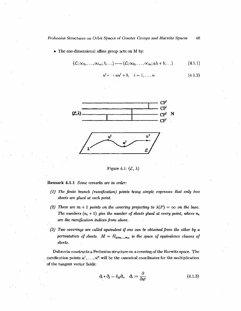
• The one-dimensional affine group acts on M by:
(£; oo0, - • •, oom; A;...) i—• (£; oo0, • • •, oom; a\ + b;...) (4.1.1)
u*>—>aui + b, i=l,...,n (4-1-2)
(CX).
CP1
CP1
CP1 N
CP1
Figure 4.1: (£, A)
Remark 4.1.1 Some remarks are in order:
(1) The finite branch (ramification) points being simple expresses that only two
sheets are glued at each point.
(2) There are m -f 1 points on the covering projecting to \{P) = oo on the base.
The numbers (n,- + 1) give the number of sheets glued at every point, where Ui
are the ramification indices from above.
(3) Two coverings are called equivalent if one can be obtained from the other by a
permutation of sheets. M = Hgrn0tm>ntn is the space of equivalence classes of
sheets.
Dubrovin constructs a Frobenius structure on a covering of the Hurwitz space. The
ramification points u1,..., un will be the canonical coordinates for the multiplication
of the tangent vector fields:
d di * dj = Sijdu di := -^ (4.1.3)

Frobenius Structures on Orbit Spaces of Coxeter Groups and Hurwitz Spaces 49
The unit vector field e and the Euler vector field E generate the action of the affine
group (4.1.2): n
e = £> (4.1-4)
n
E^^tfdi (4.1.5).
1-forms f2 on a manifold with a Frobenius algebra on the tangent planes are called
admissible if a Frobenius manifold structure is determined by the invariant inner
product:
<d',d" >n:=n(d'*d") (4.1.6)
A quadratic differential Q is called dA-divisible when it has the form Q = qdX
where the differential q has no poles in the branch points of £. The corresponding 1-
form SIQ on the Hurwitz space M is determined by any Q holomorphic for |A| < oo on
£. Since the 1-form OQ = 0, we may include also multivalued quadratic differentials
on the universal covering of £. The monodromy transformation along a cycle 7 acts
by
Q ^ Q + q^dX (4.1.7)
On a suitable covering M of M, the metrics will be defined by the 1-forms corre
sponding to these multivalued differentials Q. The covering M — Mff;no>...nm is the
space of sets
ooo,.. . , oom; A; «o, . . . , km; 0 1 , . . . , ag; (4.1.8)
with the same £,oo0, • • • > °°m a n ( i ^ from M, plus a canonical basis of cycles 0 1 , . . . , ag;
bi,...,bg on C. The branch points Pi,...,Pn are the local coordinates on M, and in
the neighbourhood of P near oo*:
k?+1{P) = \{P), P near oo*' (4.1.9)
where n* is the ramification index at 00*.
Admissible quadratic differentials on the Hurwitz space are constructed as squares
Q = <j>2 of primary differentials 4> on £ (or a covering of £). There are five types
of primary differentials. (All differentials have zero a-periods except the holomorphic
(f>si below. Also the coefficients 5,, ai,Pi,j, are independent on the point in M.) The
five types of primary differentials with their characteristic singularities are:
Frobenius Structures on Orbit Spaces of Coxeter Groups and Hurwitz Spaces 50
1. A normalized Abelian differential of the second kind:
(j) = <pti;o(P):——dkf(P), P near ool; i — 0,... ,m, a = l , . ..,«,-
(4.1.10)
2. A normalized Abelian differential of the second kind:
<(> := Sifo (4.1.11)
Mp) := -dX{P), P near oo{; i = l,...,m (4.1.12)
3. A normalized Abelian differential of the third kind:
4>:=ai<})wi{P), res0Oi(pwi = l, r e s ^ o ^ = - 1 ; i = l , . . . , m (4.1.13)
4. A normalized multivalued differential. (The differential undergoing analytic
continuation along 6fc on C tranforms as:
4> := MAP), MP + bj) - MP) = -6ijd\(P); i = l,...,9 (4.1.14)
5. A normalized holomorphic differential:
4>'=li4>+> f 4>*=&tj\ » = l,...,ff (4.1.15) Jaj
For any primary differential <f> and corresponding multivalued quadratic differential
Q = <f>2, QQ will be an admissible 1-form on the Hurwitz space M. The metric
corresponding to Q.^ is defined for two tangent fields d', d" on M as:
dS<t? = < d', d" > ^ : = n^(d' * d") (4.1.16)
This gives a Frobenius structure on M for any (f>. For the function A, a multivalued
function p on C is introduced:
p(P):=p.v. f <j> (4.1.17) Jooo
where the principal value is defined by omitting the divergent part of the integral as
a function of the local parameter ko. Now <f> = dp and A(p) on C is locally a function
Frobenius Structures on Orbit Spaces of Coxeter Groups and Hurwitz Spaces 51
of the complex variable p.

Frobenius Structures on Orbit Spaces of Coxeter Groups and Hurwitz Spaces 52
4.2 Hurwitz Spaces and Frobenius Manifolds
We now come to the main theorem of the chapter [7]:
Theorem 5 Let M be open in M and specify that <j>(Pi) ^ 0, i = 1,. ..,N. For
any primary differential (4-l-10)-(41-15), the multiplication (4-1.3), unity (4-1-4),
Euler vector field (4-1-5) and 1-form Q^2 determine on M a structure of a Frobenius
manifold. The corresponding flat coordinates tA, A = 1,...,N consist of the five
parts:
tA = (ti;a, i = 0,...,m, a = l,...,n,-; p\q\ t = l , . . . ,m; r\s\ i=l,...,g)
(4.2.1)
given by:
(4.2.2)
(4.2.3)
(4.2.4)
(4.2.5)
(4.2.6)
2.
3.
4-
5.
The metric
a.
b.
(H .16) in
f,a
P1
<t
s{ =
— resoo^ apd\
— p.v. 1 dp Jooo
= —reSootXdp
rl = <p dp
-hi** these coordinates have the (non-zero) forms:
T)ti;ati;0 =
<m .*
• i j &ij&a+0,m+\
. - 1 . . . ni + l^
(4.2.7)
(4.2.8)

Frobenius Structures on Orbit Spaces of Coxeter Groups and Hurwitz Spaces 53
c. Iris' = TT-Sij (4.2.9)
And, for any other primary differential <p, the 1-form Q^ is admissible on the Frobe
nius manifold.
Proof of the theorem.
For the multiplication (4.1.3), the metric d s | (4.1.16) is diagonal in the coordinates 1 N
u,...,uJ: dsl^r]ii{u)(dui)2 -* = 1 iV (4.2.10)
rHi = resP£- (4.2.11) aX
We now define a Darboux-Egoroff metric, then prove a lemma that for any <f>, d s |
will be Darboux-Egoroff, and will satisfy invariance conditions that give the second and fourth properties of a Frobenius manifold (definition 1.1.3).
Definition 4.2.1 A Darboux-Egoroff metric is flat, potential and diagonal. A diag
onal metric ds2 = rju(du*)2 is called potential if 3 a function V 3 diV = r)u for all i.
A potential diagonal metric is flat if the rotation coefficients jtj, i ^ j
%(«) := ^ (4.2.12)
satisfy the following for i,j,k distinct for all jij:
dklij = Hklkj (4.2.13)
n
J > 7 i i = 0 (4.2.14)
Remark 4.2.1 The rotation coefficients of the invariant metric also satisfy;
n
J2ukOklij = - 7 y (4.2.15) fc=i
Lemma 7 For any primary differential (f> listed above (4-1.10)-(4115), the metric
(4-1.16) is Darboux-Egoroff and also satisfies the invariance conditions:
Lieeds2, = 0 (4.2.16)

Frobenius Structures on Orbit Spaces of Coxeter Groups and Hurwitz Spaces 54
LieEds2^ is proportional to ds2^ (4.2.17)
The rotation coefficients of the metric do not depend on the choice of the primary
differential (f>.
Proof of the lemma:
Let za be a local parameter near ooa: za = fc"1. First, a pairing of differentials iv^\
u/2) is defined, u)^ and a/2) are holomorphic on £/(oo0 U . . . U oom), and at the
infinite points behave as:
(Where i — 1,2 and c£a, rj.„, Aa , p£.a, Qs,a are constants.)
w ( i ) - E c £ 2 a d 2 o + d E r M A f c ^ A , F - o o a (4.2.18) fe fe>0
I w® = A® (4.2.19) Jaa
w « ( F + a a ) - w » ( P ) = dpW(A), P®(A) = E P S * (4 2-2°) s>0
The bilinear pairing for UJ^\ u/2) is defined as:
(Where P0 is a marked point on £ 9 HPb) — 0)
< w w w w >:= - E a=0
E TTTct + «-i-«M»- r - (2> + 2*i „ , . r r < > fcw(2)
+ (4.2.22)
+^i E [- i ww^+i ^ w ^ + 4 ? } jfw(2)] With these definitions, the following may be proved:
Lemma 8 The following identity holds
res*> ,v = dj < w(1)o;(2> > (4.2.23)
Corollary 2 77ie pairing (4-2.22) of differentials a /^u / 2 ) is symmetric up to an
additive constant not depending on the moduli.

Frobenius Structures on Orbit Spaces of Coxeter Groups and Hurwitz Spaces 55
Prom the previous lemma, we see the rotation coefficients of the metric (4.1.16)
are symmetric:
rjjjiu) = dj<<M>>, j = l,...,N (4.2.24)
To prove the rotation coefficients satisfy (4.2.13) consider the differentia]
didj I dk4>., i, j , k, distinct (4.2.25)
which has poles only in Pi,Pj,Pk. The contour integral will be zero along a domain
DC obtained by cutting C along a canonical basis passing through FQ. Connecting
Po at a vertex of the resulting 4</-gon to the points ooo,.. -, ooTO and cutting along
these paths yields dC. The sum of the residues vanishes, and by the symmetry of the
rotation coefficients (4.2.13) is obtained, from:
djy/rfadky/rjii + 9iy/rjj]dky/fjjj = y/rjkkdidjy/rjkk (4.2.26)
Similarly, the rotation coefficients are independent of the primary differential <f>. Con
sider the differential:
d^fdjip, i^j (4.2.27)
where (p is another primary differential. Since the sum of the residues vanishes, and
the rotation coefficients are symmetric,
yfiSfryfiL = yf^fisyf& (4.2-28)
the rotation coefficients are the same for either metric. To prove (4.2.16) an operator
De on functions / = f(P,u) is defined: (and extended as the Lie derivative by
requiring dDe = Ded)
Def:=^.+def (4.2.29)
Then for any <f>,
De<t> = 0 (4.2.30)
For the metric (4.1.16), by using (4.2.24), the identity (4.2.14) is also obtained:
deVjj = 0 (4.2.31)

Frobenius Structures on Orbit Spaces of Coxeter Groups and Hurwitz Spaces 56
Similarly to prove the identity (4.2.17) an operator DE is defined:
DE:=\— + dE (4.2.32) oX
Then for any <f>,
DE4> = \<j>}4> (4.2.33)
For the primary differentials 0 listed as in (4.1.10)-(4.1.15), the numbers [4>] are given
by:
[4>A = i
[<M = o
\M = i
From this, we may write:
dE4 = (2[<t>}-l)4 (4.2.35)
which gives also (4.2.15). End proof of lemma 7.
The identity (4.2.16) is equivalent to condition (F2) from the definition (1.1.3) of the
Frobenius manifold. Also, the identity (4.2.17) is equivalent to the third condition
from (F4), equation (1.1.17). Given the Euler field (4.1.5) and multiplication (4.1.3),
the first and second conditions of (F4) equations (1.1.15), (1.1.17) are satisfied. Con
dition (F3) is given by the following lemma [7] [9]:
Lemma 9 If g is an Darboux-Egoroff metric, (with respect to the canonical coordi
nates u1,... ,un), then the Frobenius structure with canonical basis ^ has Vc sym
metric.
Since we have a Darboux-Egoroff metric for any primary differential <f> invariant with
respect to the multiplication (4.1.3), condition (F3) is satisfied. To complete the
Frobenius structure, the flat coordinates for the flat metric are established. Denote
the coordinates by tA, and define
<f>A := -dtA\dp (4.2.36)

Frobenius Structures on Orbit Spaces of Coxeter Groups and Hurwitz Spaces 57
Then by lemma (7),
< dtA,dtB >,= E r e S d A = o ^ r ^de< 4>A4>B > (4"2'37)
|A|<oo
The non-zero coefficients 4 a ' , A(a ' , qa ' for the differentials 4>A,B are as defined
in equations (4.2.18)-(4.2.21). Using De(j)B = 0 from (4.2.30):
^ = ̂ TT^-M (4-2-38) ' ^ a ~~T~ A
* r * - ^ + ( s ) , (4-2-39) de <f \4>B=f to (4.2.40)
de f </>B = - ^ ( P + 6«) + ^ ( P ) (4.2.41)
Then using the bilinear pairing (4.2.22), the forms of the metrics (4.2.7)-(4.2.9) are obtained:
m / .. na-l \
0. < MB >= - E h r r r E <3U.<fi.-i.. - (4-2-42) a=0 \ n a + 1 Jt=0 /
m -I 1 9
- E r b (*2««SU+C-V1U) - si E («i?4?+^'O o=l a a=l
End proof of the theorem.
Frobenius Structures on Orbit Spaces of Coxeter Groups and Hurwitz Spaces 58
4.3 Hurwi tz Space HQ;TI and t h e j4n-example
Example 4.3.1 The Hurwitz space H0<n corresponding to the main An-type example
consists of all polynomials of the form
A(p) =p n + 1 + anp"-1 + ... + oi, au...,aneC (4.3.1)
The affine transformations A t—> a A + b act on (4-3.1) by
p i—> a»+*p, at i—• aia~^+r~ for i > 1, Oii-> aai + b (4.3.2)
To show the Frobenius structure, we show the metric (4-2.10) is Darboux-Egoroff and
is flat for the flat coordinates. For primary differential <f> = dp, the flat coordinates
(4-2.2) correspond to the flat coordinates in example (3.1). Let us denote these flat
coordinates as£a. By an affine transformation we can set the sum of the roots to zero
and leading coefficient to one. Thus:
A(P) = (P+ & + ... +60 I I ( P - & ) (4"3-3)
a = l n n
= H(P - to) where £«, = - £ & (4-3-4) a—O a = l
Since the roots are not independent:
dlogX(p) 1
d& P ~ Co P- 6
and for the metric (3.3.7) from chapter 3:
•t = l , . . . , n (4.3.5)
<*.<W - - E — [ ( ^ - ^ ) ( ^ - j^) > ] (4.3, 6)
Then using (3.3.9) as in theorem 4,
we have for i = j :
(9(t,d(i) = respBSf0 rfdp (4.3.7) | > - £ o ) 2 A '
= 1 (4.3.8)

Frobenius Structures on Orbit Spaces of Coxeter Groups and Hurwitz Spaces 59
and for i ^ j :
( % . # & ) = reSP=io
= 2
1 A | > - 6 ) 2 A '
-,dp + resp^ 1 A
L(P-6)2A' 7dp
Giving constant coefficients:
(%,%) = 1 + fy
/or £/ie metric we denote here by g:
n
n
^(^) 2 | «o=-E?=,4i
(4.3.9)
(4.3.10)
(4.3.11)
(4.3.12)
(4.3.13)
(4.3.14) z=0
We have seen that g is Darboux-Egoroff since in canonical coordiantes w» = A(<&)
(using notations from chapter 3, theorem 4) 9 is diagonal and potential:
1 1 ftj„
with potentiality given by
where
X"(qi) (n+l)dui
1 rja S-v
X"(qi) din
n+1
(4.3.15)
(4.3.16)
(4.3.17)
(4.3.18)

Conclusion and Further
Developments
In summary, the solution space of the W D W system was shown to carry a Frobe-
nius Manifold structure, and Probenius Algebras were shown to correspond to the
matter sector of 2D-Topological Field Theories. The An example was given from the
class of polynomial solutions to W D W , and the topological Landau-Ginzburg model
was seen to correspond to the An case. We saw also how Frobenius structures are
built on the orbit spaces of Coxeter groups, and how Hurwitz Frobenius Manifolds are
constructed. The An case originally described as the unfolding of a versal singularity
was seen also to lend itself to the Coxeter orbit space construction and Hurwitz space
construction.
Frobenius structures and their prepotentials have been found on the orbit spaces of
Bn and Dn [17], in addition to that found by Dubrovin for A„ which we describe here.
It would be interesting to construct an equivariant Hurwitz space via its correspondent
metric, one which reflects the invariance of A under the action of W, and reveal further
the rather intriguing differential geometry of these Hurwitz Frobenius manifolds. This
particular problem has motivated the present write-up.
60

Bibliography
[1] Atiyah, M., The Geometry and Physics of Knots. Cambridge University Press,
Cambridge, (1990).
[2] Audin, M., An introduction to Frobenius manifolds, moduli spaces of stable maps
and quantum cohomology, Preprint Louis Pasteur University and CNRS (May
1997).
[3] Bertola M., Frobenius manifold structure on orbit space of Jacobi groups. I. Dif
ferential Geometry and its Applications 13, (2000), 19 - 41.
[4] Bertola M., Frobenius manifold structure on orbit space of Jacobi groups. II. Dif
ferential Geometry and its Applications 13, (2000), 213 - 233.
[5] Coxeter, H.S.M., Discrete groups generated by reflections, Ann. Math. 35, (1934),
588 - 621.
[6] Dubrovin B., Differential geometry of the space of orbits of a Coxeter group,
Preprint SISSA (February 1993).
[7] Dubrovin B., Geometry of 2D topological field theories, Lecture Notes in Math.
1620 (1993) 120 - 348.
[8] Hertling C , Frobenius Manifolds and Moduli Spaces for Singularities, Cambridge
Tracts in Mathematics 151, Cambridge University Press, Cambridge, (2002).
[9] Hitchin N., Frobenius manifolds. "Gauge theory and symplectic geometry (Mon
treal, 1995)," NATO Adv. Sci. Inst. Ser. C Math. Phys. Sci. 488, Kluwer, Dor
drecht (1997), 69 - 112.
[10] K. Hori et al., Mirror Symmetry American Mathematical Society, Providence,
(2003).
61

Frobenius Structures on Orbit Spaces of Coxeter Groups and Hurwitz Spaces 62
[11] Kock, J., Frobenius Algebras and 2D Topological Quantum Field Theories, Cam
bridge University Press, Cambridge, (2003).
[12] Manin, Y., Frobenius Manifolds, Quantum Cohomology, and Moduli Spaces AMS
Colloquium Publications 47, Providence, (1999).
[13] Riley, A. and Stranchan I., A Note on the Relationship between Rational and
Trigonometric Solutions of the WDVV Equations, Journal of Nonlinear Mathe
matical Physics, 14 (1) (2007): 82 - 94.
[14] Saito K., Period mappings associated to a primitive form, Publ. RIMS. 19 (1983),
1231-1264.
[15] Shramchenko, V., Deformations of Frobenius structures on Hurwitz spaces, In
ternational Mathematics Research Notices (2005) 2005(6):339 - 387.
[16] Shramchenko, V., "Real doubles" of Hurwitz Frobenius manifolds, Communica
tions in Mathematical Physics (2005) 256(3):635 - 680
[17] Zuo, D., Frobenius Manifolds Associated to Bi and Di Revisited International
Mathematics Research Notices, 2007 (20), (2007).


![Firm Frobenius monads and rm Frobenius algebras · the category of comodules over a Frobenius algebra. In [21], Frobenius algebras were treated by Street in the broader framework](https://static.fdocuments.us/doc/165x107/5f5f95d25ff49b10287be37f/firm-frobenius-monads-and-rm-frobenius-algebras-the-category-of-comodules-over-a.jpg)