Computation in Coxeter groups II. Constructing minimal rootscass/research/pdf/roots.pdf ·...
31
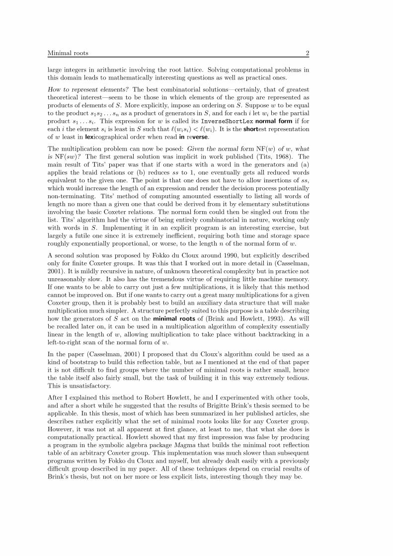
Computation in Coxeter groups II. Constructing minimal roots Bill Casselman Mathematics Department University of British Columbia Canada [email protected] Abstract. In the recent paper (Casselman, 2001) I described how a number of ideas due to Fokko du Cloux and myself could be incorporated into a reasonably efficient program to carry out multiplication in arbitrary Coxeter groups. At the end of that paper I discussed how this algorithm could be used to build the reflection table of minimal roots, which could in turn form the basis of a much more efficient multiplication algorithm. In this paper, following a suggestion of Robert Howlett, I explain how results due to Brigitte Brink can be used to construct the minimal root reflection table directly and more efficiently. Introduction A Coxeter system is a pair (W, S ) where W is a group with a set of generators S and relations (st) ms,t =1 for pairs s, t in S, with the conditions that m s,s = 1 and 2 ≤ m s,t ≤∞ for s = t. In this paper I shall always assume S to be finite. Equivalent to these are the relations s 2 =1 sts ...= tst ... (m s,t terms on each side) The second type are called braid relations. Often the group alone is referred to, but al- most always when one refers to a Coxeter group one has in mind a particular set S. The relations involved here are very simple, but these systems play an extremely important role in mathematics, one far from visible in the bare definition. Among other things, the Weyl groups of Kac-Moody Lie algebras possess a natural structure as a Coxeter system. Much work has been done on these structures, particularly on finite and affine Weyl groups, but many phenomena involving them remain unexplained, and it is likely that computer explo- rations will be even more significant in the future than they have been so far. These groups become extremely complex as the size of S grows, however, and computer programs dealing with them must be extremely efficient to be useful. Conventional symbolic algebra packages normally fail to handle the difficulties satisfactorily. This paper is the second of a series in which I describe what may be even in the long term the most efficient algorithms to do basic computations in arbitrary Coxeter groups, at least on serial machines. These algorithms depend strongly on mathematical results of Brigitte Brink, Robert Howlett, and Fokko du Cloux. The most basic problems are those one encounters immediately: (1) how to represent el- ements of the group and (2) how to multiply two elements if they are given in whatever format has been chosen? These two problems are of course strongly related, and are by no means simple matters. For familiar examples such as S n there are many satisfactory methods, and for the Weyl groups of Kac-Moody algebras one can use the representation of the group on the root lattice to reduce many problems to integer arithmetic. But arbitrary groups, even sometimes the exceptional finite groups H 3 and H 4 , are computationally more demanding. Even when working with Weyl groups one should be prepared to deal with very
Transcript of Computation in Coxeter groups II. Constructing minimal rootscass/research/pdf/roots.pdf ·...
Computation in Coxeter groups II. Constructing minimal roots
Bill CasselmanMathematics DepartmentUniversity of British [email protected]
Abstract. In the recent paper (Casselman, 2001) I described how a number of ideas dueto Fokko du Cloux and myself could be incorporated into a reasonably efficient program tocarry out multiplication in arbitrary Coxeter groups. At the end of that paper I discussedhow this algorithm could be used to build the reflection table of minimal roots, which couldin turn form the basis of a much more efficient multiplication algorithm. In this paper,following a suggestion of Robert Howlett, I explain how results due to Brigitte Brink canbe used to construct the minimal root reflection table directly and more efficiently.
Introduction
A Coxeter system is a pair (W, S) where W is a group with a set of generators S andrelations
(st)ms,t = 1
for pairs s, t in S, with the conditions that ms,s = 1 and 2 ≤ ms,t ≤ ∞ for s 6= t. In thispaper I shall always assume S to be finite. Equivalent to these are the relations
s2 = 1
sts . . . = tst . . . (ms,t terms on each side)
The second type are called braid relations. Often the group alone is referred to, but al-most always when one refers to a Coxeter group one has in mind a particular set S. Therelations involved here are very simple, but these systems play an extremely important rolein mathematics, one far from visible in the bare definition. Among other things, the Weylgroups of Kac-Moody Lie algebras possess a natural structure as a Coxeter system. Muchwork has been done on these structures, particularly on finite and affine Weyl groups, butmany phenomena involving them remain unexplained, and it is likely that computer explo-rations will be even more significant in the future than they have been so far. These groupsbecome extremely complex as the size of S grows, however, and computer programs dealingwith them must be extremely efficient to be useful. Conventional symbolic algebra packagesnormally fail to handle the difficulties satisfactorily. This paper is the second of a series inwhich I describe what may be even in the long term the most efficient algorithms to do basiccomputations in arbitrary Coxeter groups, at least on serial machines. These algorithmsdepend strongly on mathematical results of Brigitte Brink, Robert Howlett, and Fokko duCloux.
The most basic problems are those one encounters immediately: (1) how to represent el-ements of the group and (2) how to multiply two elements if they are given in whateverformat has been chosen? These two problems are of course strongly related, and are byno means simple matters. For familiar examples such as Sn there are many satisfactorymethods, and for the Weyl groups of Kac-Moody algebras one can use the representation ofthe group on the root lattice to reduce many problems to integer arithmetic. But arbitrarygroups, even sometimes the exceptional finite groups H3 and H4, are computationally moredemanding. Even when working with Weyl groups one should be prepared to deal with very
Minimal roots 2
large integers in arithmetic involving the root lattice. Solving computational problems inthis domain leads to mathematically interesting questions as well as practical ones.
How to represent elements? The best combinatorial solutions—certainly, that of greatesttheoretical interest—seem to be those in which elements of the group are represented asproducts of elements of S. More explicitly, impose an ordering on S. Suppose w to be equalto the product s1s2 . . . sn as a product of generators in S, and for each i let wi be the partialproduct s1 . . . si. This expression for w is called its InverseShortLex normal form if foreach i the element si is least in S such that ℓ(wisi) < ℓ(wi). It is the shortest representationof w least in lexicographical order when read in reverse.
The multiplication problem can now be posed: Given the normal form NF(w) of w, whatis NF(sw)? The first general solution was implicit in work published (Tits, 1968). Themain result of Tits’ paper was that if one starts with a word in the generators and (a)applies the braid relations or (b) reduces ss to 1, one eventually gets all reduced wordsequivalent to the given one. The point is that one does not have to allow insertions of ss,which would increase the length of an expression and render the decision process potentiallynon-terminating. Tits’ method of computing amounted essentially to listing all words oflength no more than a given one that could be derived from it by elementary substitutionsinvolving the basic Coxeter relations. The normal form could then be singled out from thelist. Tits’ algorithm had the virtue of being entirely combinatorial in nature, working onlywith words in S. Implementing it in an explicit program is an interesting exercise, butlargely a futile one since it is extremely inefficient, requiring both time and storage spaceroughly exponentially proportional, or worse, to the length n of the normal form of w.
A second solution was proposed by Fokko du Cloux around 1990, but explicitly describedonly for finite Coxeter groups. It was this that I worked out in more detail in (Casselman,2001). It is mildly recursive in nature, of unknown theoretical complexity but in practice notunreasonably slow. It also has the tremendous virtue of requiring little machine memory.If one wants to be able to carry out just a few multiplications, it is likely that this methodcannot be improved on. But if one wants to carry out a great many multiplications for a givenCoxeter group, then it is probably best to build an auxiliary data structure that will makemultiplication much simpler. A structure perfectly suited to this purpose is a table describinghow the generators of S act on the minimal roots of (Brink and Howlett, 1993). As willbe recalled later on, it can be used in a multiplication algorithm of complexity essentiallylinear in the length of w, allowing multiplication to take place without backtracking in aleft-to-right scan of the normal form of w.
In the paper (Casselman, 2001) I proposed that du Cloux’s algorithm could be used as akind of bootstrap to build this reflection table, but as I mentioned at the end of that paperit is not difficult to find groups where the number of minimal roots is rather small, hencethe table itself also fairly small, but the task of building it in this way extremely tedious.This is unsatisfactory.
After I explained this method to Robert Howlett, he and I experimented with other tools,and after a short while he suggested that the results of Brigitte Brink’s thesis seemed to beapplicable. In this thesis, most of which has been summarized in her published articles, shedescribes rather explicitly what the set of minimal roots looks like for any Coxeter group.However, it was not at all apparent at first glance, at least to me, that what she does iscomputationally practical. Howlett showed that my first impression was false by producinga program in the symbolic algebra package Magma that builds the minimal root reflectiontable of an arbitrary Coxeter group. This implementation was much slower than subsequentprograms written by Fokko du Cloux and myself, but already dealt easily with a previouslydifficult group described in my paper. All of these techniques depend on crucial results ofBrink’s thesis, but not on her more or less explicit lists, interesting though they may be.
Minimal roots 3
This paper will explain in detail an elaboration of Howlett’s idea of how to apply the resultsof Brink’s thesis to practical programming in order to construct the minimal roots. Theresulting program will not be the fastest possible, but it will be fairly fast. Howlett’s Magmaprogram took a little over an hour to handle it, he tells me, whereas a program in C writtenby Fokko du Cloux took 10 seconds on a comparable machine. The version based on thetechnique to be given here lies in between the two—a version written in Java took a bitless than a minute on the same machine as that used by du Cloux. The principal drawbackof the algorithm to be presented here as the basis of multiplication is that it claims anamount of machine memory proportional to the number of minimal roots. The number ofminimal roots can grow quite fast with the size of S, so this is not a negligible objection.It thus exemplifies the usual programming trade-off between time and space. FamiliarCoxeter groups are deceptive in this regard—for classical series of finite and affine groupsthe number of minimal roots is roughly proportional to |S|2, whereas one of the first reallydifficult groups Howlett’s program dealt with was an exotic Coxeter group with |S| = 22and several hundred thousand minimal roots. Groups for which the set of minimal roots islarge are so complicated that there is not much exploration one can expect to do with themanyway, and in practice the number of minimal roots is only a relatively minor impediment.
I begin this paper recalling the basic properties of minimal roots; explain how they are tobe used in multiplication; summarize results of Brigitte Brink’s thesis in the manner mostuseful for my purposes; and finally explain how to apply these results in practice to constructthe minimal root reflection table. I should say that what I am going to come up with issomewhat different from Howlett’s program, and also quite different from a closely relatedprogram of Fokko du Cloux. It uses a few more advanced features of Brink’s thesis thanHowlett’s program. It is less sophisticated than du Cloux’s program, but has the advantageof being possibly clearer in conception.
Once Howlett had suggested using the results of Brink’s thesis, the path to a practicalprogram was in principle not too difficult. On the other hand, this path did not appearobvious to me until after a great deal of exploration, and it will surely be useful to place herea record of the outcome. This paper is largely self-contained; the order of exposition andits occasional geometric emphasis are new. My principal ambition in writing it has been toawaken interest in the work of Brink, Howlett, and du Cloux. This whole area of researchis one of great charm, but it has apparently and unfortunately awakened little interest atlarge. This is likely due to the fact that it lies somewhere in the great no man’s landbetween pure mathematics and practical computation—terra incognita on most maps, evenin the 21st century. I must also record that both my programs and this exposition benefitedenormously from conversations with the late and very much lamented Fokko du Cloux. AsI learned long ago to my own chagrin, competing directly in programming with him couldbe an embarrassing experience, but working alongside him was always, on the contrary, atonce enjoyable and educational. With his death went a uniquely talented mathematician.
§§1–3 will recall some of the basic geometry of Coxeter groups, and §4 will recall how minimalroots can be used in multiplication. In §5 I start discussing the algorithm itself, with detailspresented in §§6–9.
1. The geometry of roots
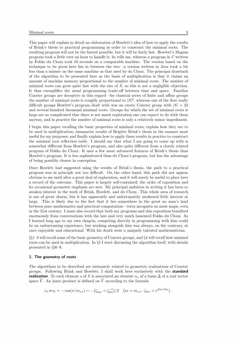
The algorithms to be described are intimately related to geometric realizations of Coxetergroups. Following Brink and Howlett, I shall work here exclusively with the standardrealization. To each element s of S is associated an element αs of a basis ∆ of a real vectorspace V . An inner product is defined on V according to the formula
αs •αt = − cos(π/ms,t) = −(ζ2m + ζ−1
2m
)/2
(m = ms,t, ζ2m = e2πi/2m
).
Minimal roots 4
In particular, αs •αs = 1 for all s. The angle π/∞ is to be interpreted as 0.
In the dual V of V vectors α∨ are then defined by the conditions
〈α, β∨〉 = 2 (α •β) .
The α∨ (for α in ∆∨) may not be linearly independent. This is so when the matrix α •β issingular, as for example when it is [
1 −1−1 1
]
and α∨ = −β∨. For each s in S reflections in V are defined by the formulas
sv = v − 〈αs, v〉α∨s .
Dual reflections in V are defined by the formulas
〈sλ, v〉 = 〈λ, sv〉
so thatsλ = λ − 〈λ, α∨
s 〉αs = λ − 2 (λ •αs)αs .
These reflections preserve the inner product. Thus, assuming s 6= t, we have αs •αt = −1whenever s and t generate an infinite group, αs •αt = 0 when s and t commute, and−1 < αs •αt ≤ −1/2 otherwise. The maps taking the elements s to the corresponding
reflections induce homomorphisms of W into both GL(V ) and GL(V ).
The Coxeter graph associated to a Coxeter system has as nodes the elements of S, and anedge linking s and t if ms,t, which is called the degree of the edge, is more than 2. In otherwords, the edges link s and t with αs •αt 6= 0. In this case—i.e. when α •β 6= 0—I writeα ∼ β. A simple link in the graph is one with degree 3, a multiple link one of higher degree.The formula for reflection amounts to the specification that if λ =
∑λγγ and s = sα
(sλ)β =
{−λα +
∑α∼γ [−2 α • γ] λγ if β = α
λβ otherwise
In calculations, it is frequently best to work with 〈α, β∨〉 = 2 α •β rather than the dot-product itself, since it is at once simpler and more efficient to do so.
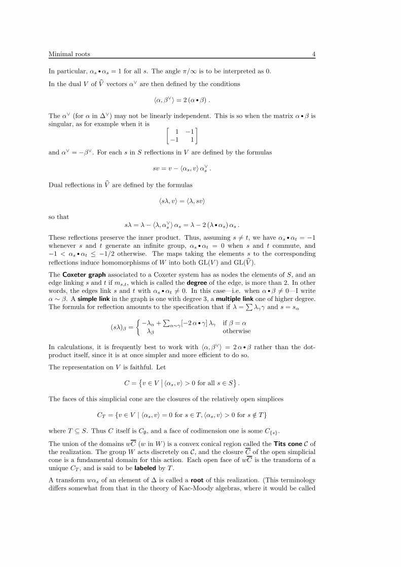
The representation on V is faithful. Let
C ={v ∈ V
∣∣ 〈αs, v〉 > 0 for all s ∈ S}
.
The faces of this simplicial cone are the closures of the relatively open simplices
CT = {v ∈ V | 〈αs, v〉 = 0 for s ∈ T, 〈αs, v〉 > 0 for s /∈ T }
where T ⊆ S. Thus C itself is C∅, and a face of codimension one is some C{s}.
The union of the domains wC (w in W ) is a convex conical region called the Tits cone C ofthe realization. The group W acts discretely on C, and the closure C of the open simplicialcone is a fundamental domain for this action. Each open face of wC is the transform of aunique CT , and is said to be labeled by T .
A transform wαs of an element of ∆ is called a root of this realization. (This terminologydiffers somewhat from that in the theory of Kac-Moody algebras, where it would be called
Minimal roots 5
a real root.) Points in the root hyperplane λ = 0 are fixed by the root reflection sλ whereswα = wsαw−1, the conjugate of an element in S. For any root λ, define
Cλ=0 = {v ∈ C | 〈λ, v〉 = 0}Cλ≥0 = {v ∈ C | 〈λ, v〉 ≥ 0}Cλ≤0 = {v ∈ C | 〈λ, v〉 ≤ 0} .
The collection of root hyperplanes is locally finite in C.
A root λ is called positive if λ > 0 on C, negative if λ < 0 on C. Every root is eitherpositive or negative, which means that no root hyperplane ever intersects C. A root λ ispositive if and only if λ =
∑α∈∆ λαα with all λα ≥ 0.
1.1. Proposition. Suppose λ and µ to be distinct positive roots. The following are equiva-lent:
(a) λ •µ = cos(πk/ms,t) with 0 < k < ms,t for some s, t in S with ms,t < ∞;(b) |λ •µ| < 1;(c) the group generated by the root reflections sλ and sµ is finite;(d) the hyperplanes λ = 0 and µ = 0 intersect in the interior of C;(e) there exists a point of C in the region where λ < 0 and µ < 0;(f) there exists a point of V in the region where λ > 0 and µ > 0 whose orbit under the
group generated by sλ and sµ contains a point in the region where λ < 0 and µ < 0.
PROOF. This is implicit in the very early article (Vinberg, 1971). That (a) implies (b) istrivial; that (b) implies (c) is a consequence of the simplest part of his discussion of pairs ofreflections. If G is any finite subgroup of W then the G-orbit of any point in the interior ofC will be finite, and since C is convex the centre of mass of the orbit will be in the interiorof C as well. This shows that (c) implies (d). Suppose L = {λ = 0} ∩ {µ = 0} to containa point in the interior of C. The whole of C is tiled by simplices wCT . Points in the opencones wC are fixed only by 1 in W , and those in some wC{s} are fixed only by 1 and a singlereflection. Therefore the linear space L must contain some wCT with |T | = 2. This meansthat s and t can be simultaneously conjugated into WT , and shows that (d) implies (a).
That (d) implies (e) is trivial.
To show that (e) implies (f), let P be a point in C where λ < 0 and µ < 0. We may assumethat P is in the interior of C. If Q is a point of C, the segment from P to Q intersects only afinite number of root hyperplanes, which means that there are only a finite number of roothyperplanes separating P from C. But if κ is any positive root and 〈κ, P 〉 < 0 then P lieson the side of κ = 0 away from C, while sκP lies on the same side. So a finite number ofapplications of sλ and sµ to P will bring it to the region where λ > 0, µ > 0.
It remains to show that (f) implies (c). In effect, this hypothesis means that the group hasa longest element. This is a standard argument, which I’ll not repeat here. QED
Following Brink and Howlett, I say that the positive root λ dominates the positive root µif the region Cλ≥0 contains the region Cµ≥0. Another way of putting this is to require thatλ > 0 in every chamber wC on which µ > 0.
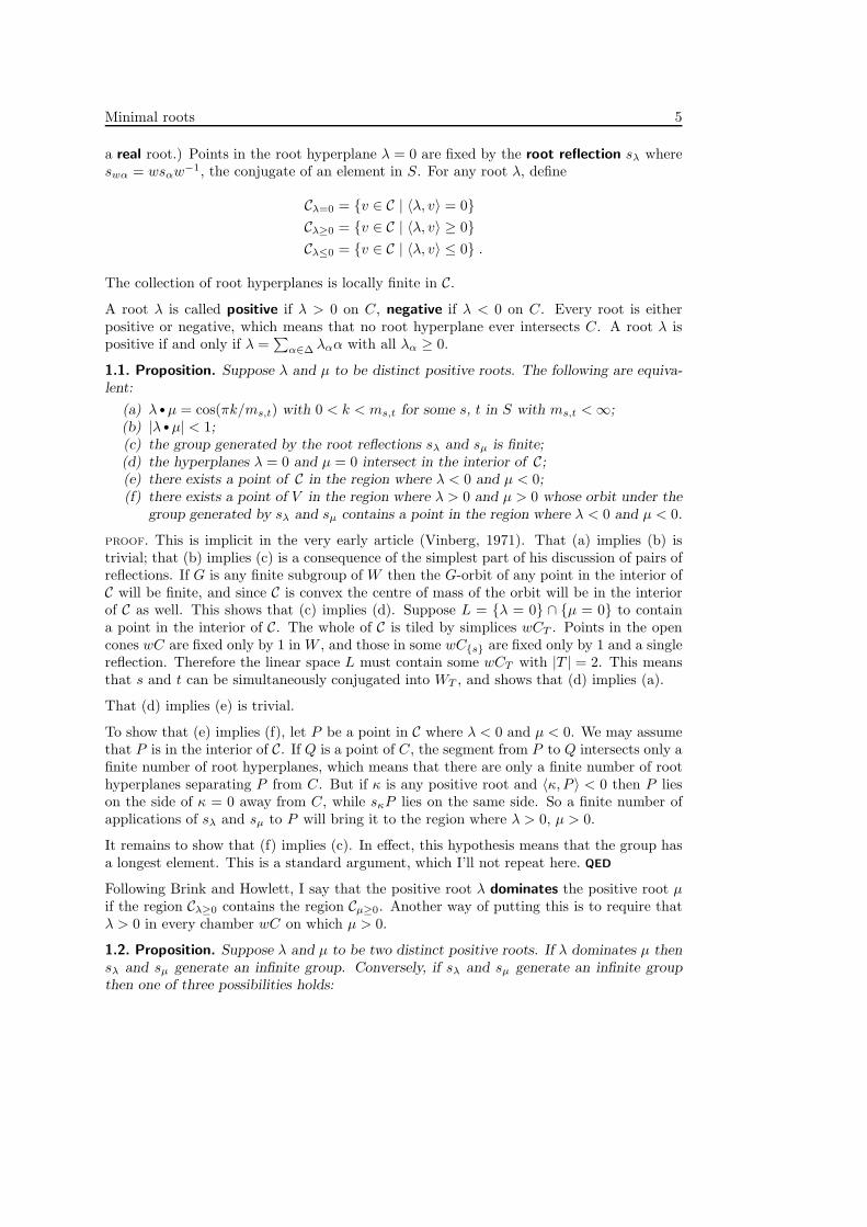
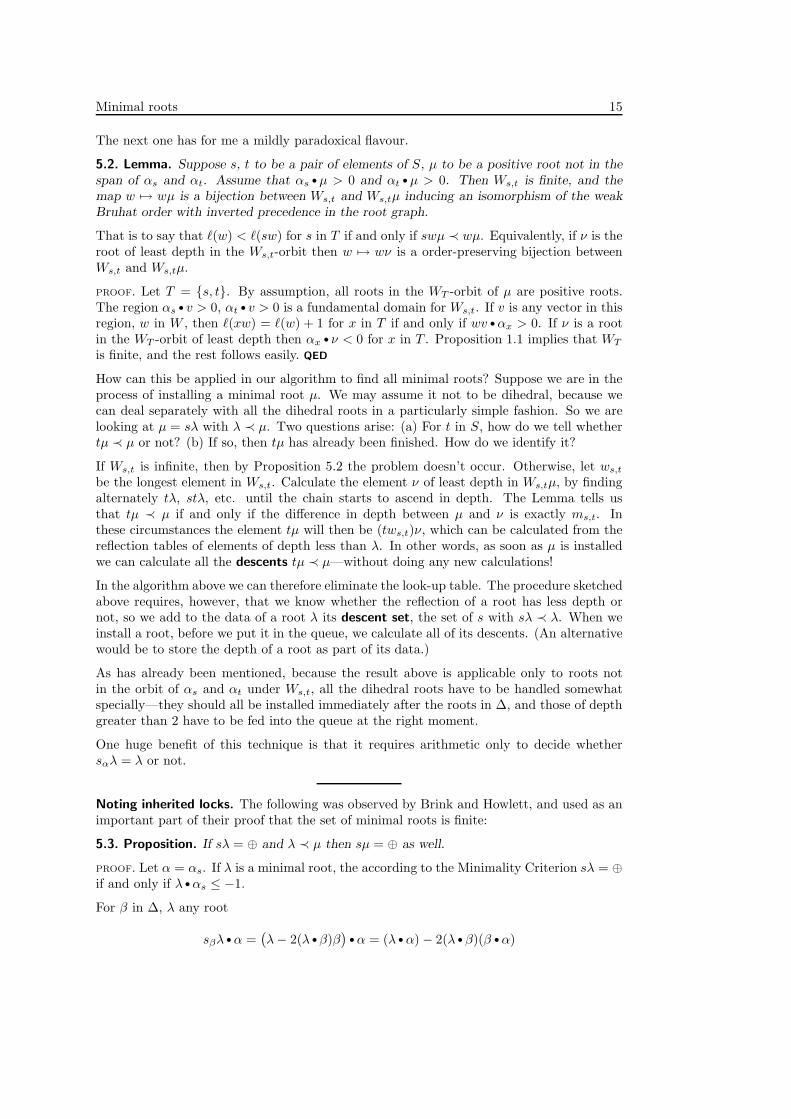
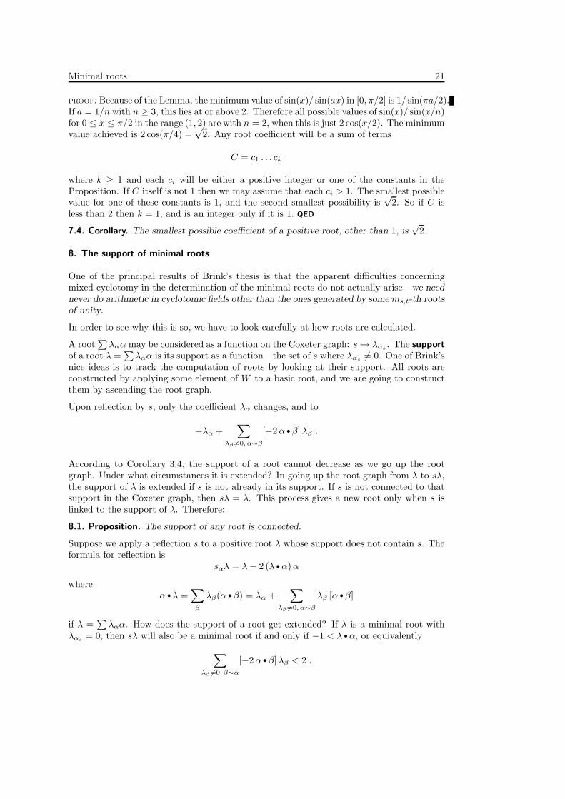
1.2. Proposition. Suppose λ and µ to be two distinct positive roots. If λ dominates µ thensλ and sµ generate an infinite group. Conversely, if sλ and sµ generate an infinite groupthen one of three possibilities holds:
Minimal roots 6
(a) λ dominates µ;(b) µ dominates λ;(c) sµλ dominates µ and sλµ dominates λ.
PROOF. For any root λ, let {λ = 0}int be the intersection of the hyperplane λ = 0 with theinterior of C. According to Proposition 1.1, that the pair sλ and sµ generate an infinitegroup means neither more nor less than that
{λ = 0}int ∩ {µ = 0}int = ∅ .
Suppose that λ dominates µ, so that Cµ≥0 is contained in Cλ≥0. Since λ and µ are distinct,the hyperplanes λ = 0 and µ = 0 are distinct. The intersection of the two hyperplanes hascodimension one in either of them. If P lies in the intersection {λ = 0}int ∩ {µ = 0}int thenthere will exist points in the interior of C where µ = 0 and λ is negative. This contradictsthe dominance of µ by λ. From this we conclude that if λ dominates µ then sλ and sµ
generate an infinite group.
Suppose that sλ and sµ generate an infinite group. Since
{λ = 0}int ∩ {µ = 0}int = ∅ ,
the sign of µ on {λ = 0}int is a non-zero constant, as is that of λ on {µ = 0}int.
Suppose that λ < 0 on {µ = 0}int. I claim that in this case µ dominates λ. If not, thenthere exists a point P in C where λ ≥ 0 but µ < 0. If Q lies in the interior of C the opensegment QP must lie entirely in the convex set where λ ≥ 0 as well as the interior of C.It crosses from the region where µ > 0 to that where µ < 0, and must therefore contain apoint where µ = 0 but λ ≥ 0, a contradiction.
Similarly, if λ > 0 on {µ = 0}int and µ < 0 on {λ = 0}int then λ dominates µ.
Finally, suppose that λ > 0 on {µ = 0}int, and that µ > 0 on {λ = 0}int. I claim that µ > 0on sλC. If not, then µ < 0 on sλC. If P lies in sλC and Q lies on {λ = 0}int then on theone hand λ < 0 on [P, Q) while on the other 〈µ, P 〉 < 0 while 〈µ, Q〉 > 0 so µ = 0 for somepoint of (P, Q), contradicting the assumption that λ > 0 on {µ = 0}int. But since µ > 0 onsλC, sλµ > 0 on C and sλµ is a positive root. But λ < 0 on sλ{µ = 0} so if we replace µby sλµ we are back in the first case. Similarly for sµλ. QED
The three cases are shown in these figures:
µ=
0
λ = 0
λ=
0
µ = 0
λ=
0
µ=
0
Minimal roots 7
2. Minimal roots
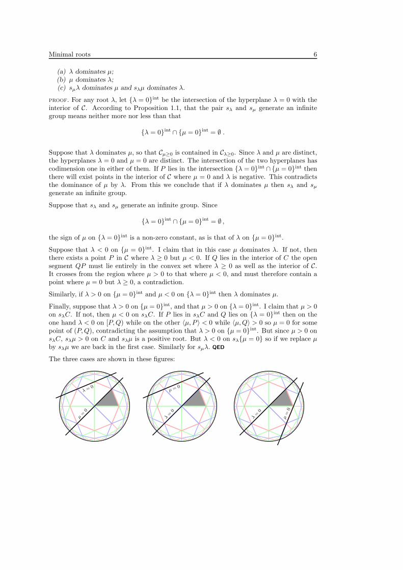
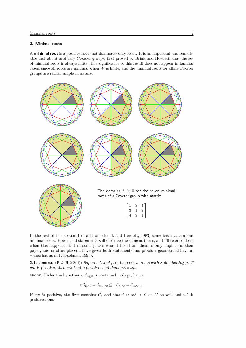
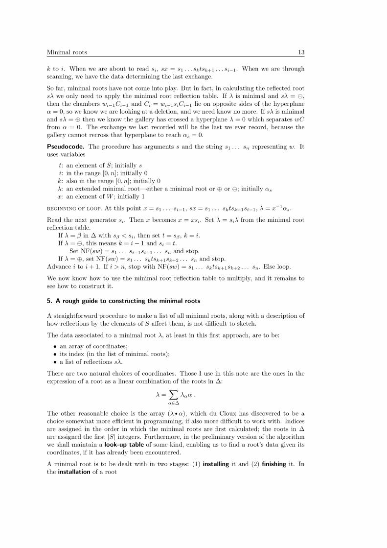
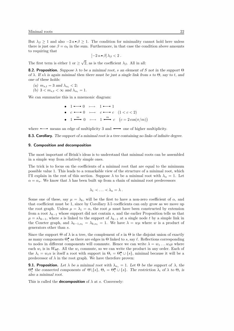
A minimal root is a positive root that dominates only itself. It is an important and remark-able fact about arbitrary Coxeter groups, first proved by Brink and Howlett, that the setof minimal roots is always finite. The significance of this result does not appear in familiarcases, since all roots are minimal when W is finite, and the minimal roots for affine Coxetergroups are rather simple in nature.
The domains λ ≥ 0 for the seven minimal
roots of a Coxeter group with matrix
1 3 43 1 34 3 1
In the rest of this section I recall from (Brink and Howlett, 1993) some basic facts aboutminimal roots. Proofs and statements will often be the same as theirs, and I’ll refer to themwhen this happens. But in some places what I take from them is only implicit in theirpaper, and in other places I have given both statements and proofs a geometrical flavour,somewhat as in (Casselman, 1995).
2.1. Lemma. (B & H 2.2(ii)) Suppose λ and µ to be positive roots with λ dominating µ. Ifwµ is positive, then wλ is also positive, and dominates wµ.
PROOF. Under the hypothesis, Cµ≥0 is contained in Cλ≥0, hence
wCµ≥0 = Cwµ≥0 ⊆ wCλ≥0 = Cwλ≥0 .
If wµ is positive, the first contains C, and therefore wλ > 0 on C as well and wλ ispositive.. QED
Minimal roots 8
It is well known that s in S permutes the complement of αs in the set of all positive roots,or in other words that if s is in S and λ a positive root, then either λ = αs and sλ < 0, orsλ > 0. For the minimal roots, there is a similar range of options:
2.2. Proposition. If λ is a minimal root and s in S then exactly one of these three optionsholds:
• λ = αs and sλ < 0;• sλ is again minimal;• sλ dominates αs.
PROOF. If λ 6= αs > 0, then sλ > 0. If sαλ is not minimal, say it dominates β > 0 withsλ 6= β. If β 6= α, then sαβ > 0, and by the previous Lemma λ = sαsαλ dominates sαβ.Since λ is minimal, this can only happen if λ = sαβ, a contradiction. QED
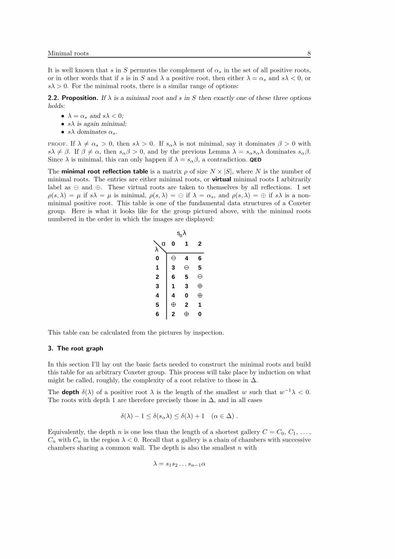
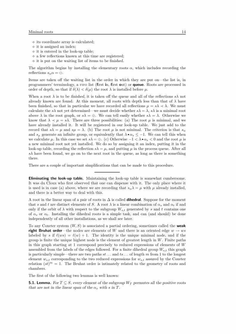
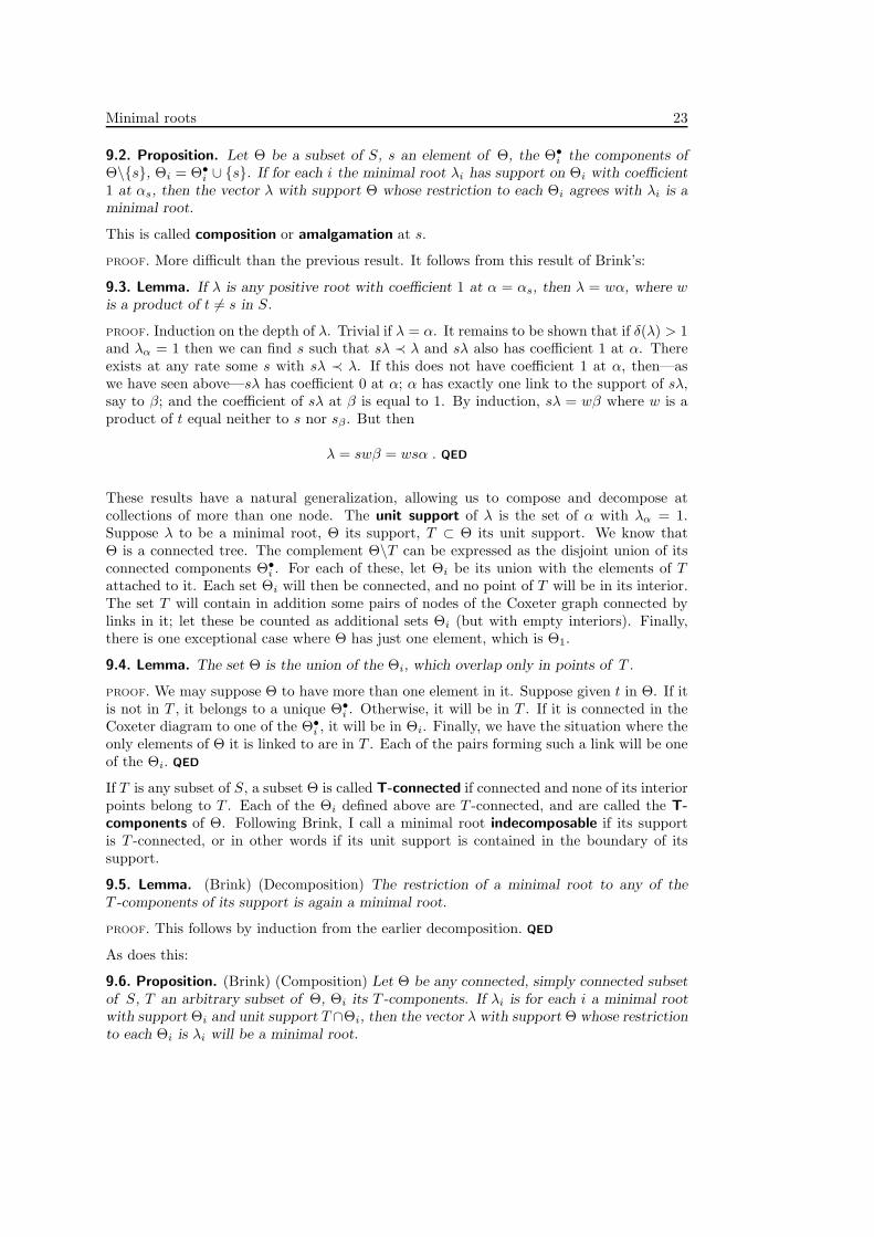
The minimal root reflection table is a matrix ρ of size N × |S|, where N is the number ofminimal roots. The entries are either minimal roots, or virtual minimal roots I arbitrarilylabel as ⊖ and ⊕. These virtual roots are taken to themselves by all reflections. I setρ(s, λ) = µ if sλ = µ is minimal, ρ(s, λ) = ⊖ if λ = αs, and ρ(s, λ) = ⊕ if sλ is a non-minimal positive root. This table is one of the fundamental data structures of a Coxetergroup. Here is what it looks like for the group pictured above, with the minimal rootsnumbered in the order in which the images are displayed:
0 1 2
0
2 0
1
2 1
2
4 0
3 1 3
4
6 5
5
3 5
6
4 6λ
αsαλ
This table can be calculated from the pictures by inspection.
3. The root graph
In this section I’ll lay out the basic facts needed to construct the minimal roots and buildthis table for an arbitrary Coxeter group. This process will take place by induction on whatmight be called, roughly, the complexity of a root relative to those in ∆.
The depth δ(λ) of a positive root λ is the length of the smallest w such that w−1λ < 0.The roots with depth 1 are therefore precisely those in ∆, and in all cases
δ(λ) − 1 ≤ δ(sαλ) ≤ δ(λ) + 1 (α ∈ ∆) .
Equivalently, the depth n is one less than the length of a shortest gallery C = C0, C1, . . . ,Cn with Cn in the region λ < 0. Recall that a gallery is a chain of chambers with successivechambers sharing a common wall. The depth is also the smallest n with
λ = s1s2 . . . sn−1α

Minimal roots 9
for some α ∈ ∆. A partial order is thus induced on the set of all positive roots: λ � µ ifµ = wλ where δ(µ) = ℓ(w) + δ(λ). This order gives rise to the root graph, whose nodes arepositive roots, with edges λ → sλ whenever λ ≺ sλ.
3.1. Lemma. If λ and µ are distinct positive roots and sµλ dominates µ then sµλ > 0 andδ(λ) < δ(sµλ).
λ = 0
µ = 0
sµλ = 0
C
λ = 0
µ = 0
sµλ = 0
C
PROOF. If (Ci) is a gallery of least length from C to the region where sµλ < 0, there will besome pair Ci, Ci+1 sharing a wall on the hyperplane µ = 0. The gallery reflected at µ = 0will be shorter. Hence δ(λ) < δ(sµλ). QED
The minimal roots lie at the bottom of the root graph, in the sense that:
3.2. Proposition.(B & H 2.2(iii)
)If λ and µ are both positive roots with λ � µ and µ is
minimal, so is λ.
PROOF. This reduces to the case µ = sαλ. If µ is minimal but µ 6= α, then either sαµ = λ isminimal, or it dominates α. But by the preceding Lemma, in the second case δ(µ) < δ(sαµ),a contradiction. QED
3.3. Lemma. (B & H 2.3) If λ > 0 and λ •α > 0 then sαλ ≺ λ.
PROOF. Suppose w−1λ < 0 with ℓ(w) = δ(λ).
If w−1α < 0 then we can write
w = sαs2 . . . sn
λ = sαs2 . . . sn−1αn (αn = αss)
sαλ = s2 . . . sn−1αn
δ(sαλ) = n − 1 < δ(λ) = n .
Now assume that w−1α > 0. Let w have the reduced expression w = s1 . . . sn, and letu = wsn = s1 . . . sn−1. Thus wαn < 0. I claim that u−1sαλ < 0, which implies thatδ(sαλ) = n − 1.
We can calculate thatw−1sαλ = w−1λ − 2 (λ •α)w−1α
u−1sαλ = snw−1sαλ
= sn(w−1λ − 2 (λ •α)w−1α)
= u−1λ − 2 (λ •α)snw−1α .
Since the depth of λ is n, µ = u−1λ will be positive. But then µ > 0, snµ < 0 implies thatµ = αn. So we have
u−1sαλ = αn − 2 (λ •α)snw−1α .
Minimal roots 10
The rootαn − 2 (λ •α)snw−1α
is either positive or negative. In the second term, the positive root w−1α cannot be αn,since then α = wαn, contradicting wαn < 0. Therefore snw−1α is a positive root also notαn, and the second term is a negative root not equal to a multiple of −αn. The whole sumtherefore has to be negative. QED
3.4. Corollary. (B & H 1.7) Whenever λ is a positive root and s in S with λ 6= αs there arethree possibilities: (a) sλ ≺ λ, (b) sλ = λ, or (c) λ ≺ sλ, depending on whether λ •αs > 0,λ •αs = 0, or λ •αs < 0, respectively.
3.5. Corollary. (B & H 1.8) If λ =∑
λαα � µ =∑
µαα then λα ≤ µα.
In constructing the list of minimal roots and the minimal root reflection table, the roots willbe dealt with by going up the root graph. We shall find ourselves in the situation where λis a minimal root and we know all sλ ≺ λ. We are to calculate an unknown sλ. We haveto decide whether sαλ is again minimal or not. It is easy to decide whether λ = α, and inthe remaining cases the possibilities, according to Proposition 2.2, are that it is minimal orthat sαλ dominates α. How do we tell which?
3.6. Proposition. Suppose α to lie in ∆, λ to be a minimal root distinct from α. If λ ≺ sαλthen sαλ is again minimal if and only if sα and sλ generate a finite group.
Or, equivalently, sαλ is not minimal if and only if sα and sλ generate an infinite group.
PROOF. Let µ = sαλ.
Suppose that µ is not minimal. Then it dominates α, and sα and sµ generate an infinitegroup. But this is also the group generated by sλ and sα.
Conversely, suppose sµ and sα generate an infinite group. Among the three possibilities ofProposition 1.2 only the one in which µ dominates α is possible, since λ ≺ µ. QED
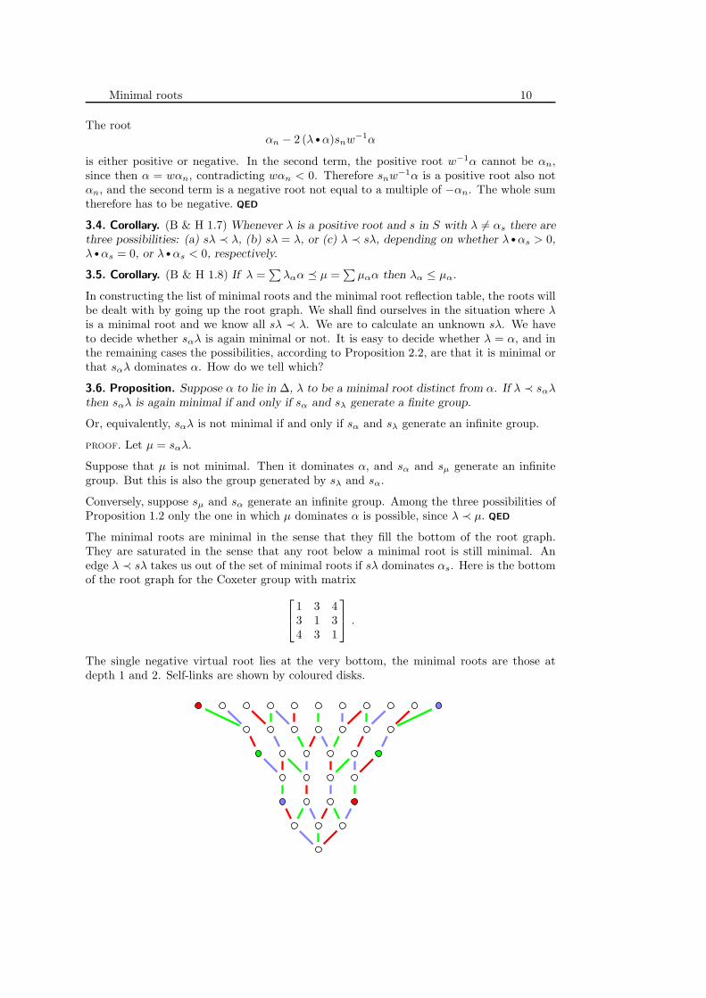
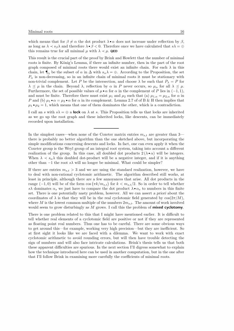
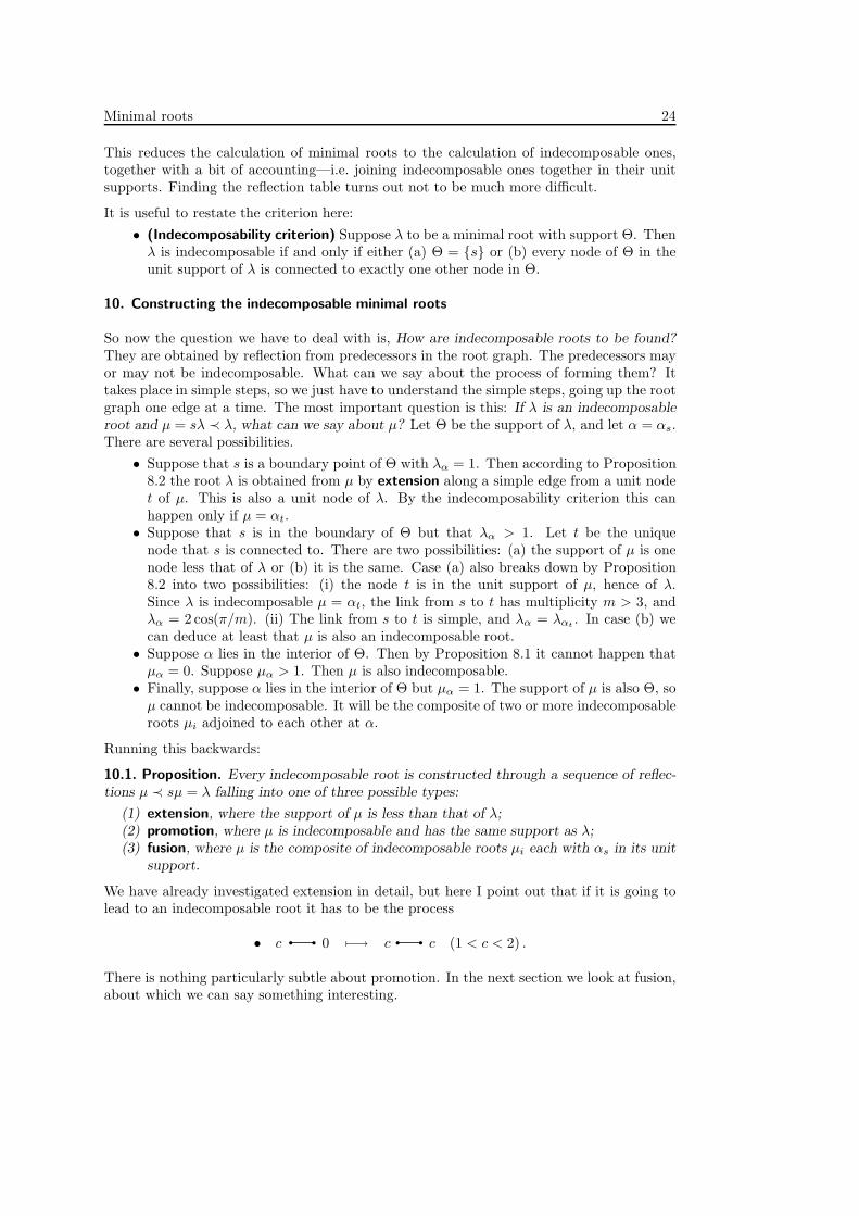
The minimal roots are minimal in the sense that they fill the bottom of the root graph.They are saturated in the sense that any root below a minimal root is still minimal. Anedge λ ≺ sλ takes us out of the set of minimal roots if sλ dominates αs. Here is the bottomof the root graph for the Coxeter group with matrix
1 3 43 1 34 3 1
.
The single negative virtual root lies at the very bottom, the minimal roots are those atdepth 1 and 2. Self-links are shown by coloured disks.

Minimal roots 11
These results will soon be used to outline an algorithm to construct the minimal rootreflection table. Processing roots will take place in order of increasing depth, applying this:
Minimality Criterion: If λ 6= α is a minimal root and λ ≺ sαλ, then sαλ is nolonger a minimal root if and only if λ •αs ≤ −1.
Details follow, after I explain in the next section how to use the minimal root reflectiontable in multiplication.
4. Minimal roots and multiplication
Suppose w to have the normal form w = s1 . . . sn. Then according to du Cloux’s strongform of the exchange principle (explained first in (du Cloux, 1990) and more generally in(Casselman, 2001)) the normal form of sw will be obtained from that of w by either insertionor deletion:
NF(sw) = s1 . . . sitsi+1 . . . sn
orNF(sw) = s1 . . . si−1si+1 . . . sn .
How do we find which of the two is concerned, and where the insertion or deletion occurs?If insertion, which t is to be inserted?
The algorithm explained in (Casselman, 2001) handles these problems in geometric terms. Idefine the InverseShortLex tree to be the directed graph whose nodes are elements of W ,with a link from x to y labeled by s if NF(y) = NF(x)•s. Its root is the identity element.Each y 6= 1 in W is the target of exactly one link, labeled by the s in S least with ys < y.Paths in this tree starting at 1 match the normal forms of elements of W .
The InverseShortLex tree for A2
This tree gives rise to a geometrical figure in which we put a link from xC to yC if there isan edge in the tree from x to y. The multiplication problem can now be formulated: givenan InverseShortLex path from C to wC, how can we find the InverseShortLex path fromC to swC? As explained in (Casselman, 2001), the InverseShortLex figure is very close to
Minimal roots 12
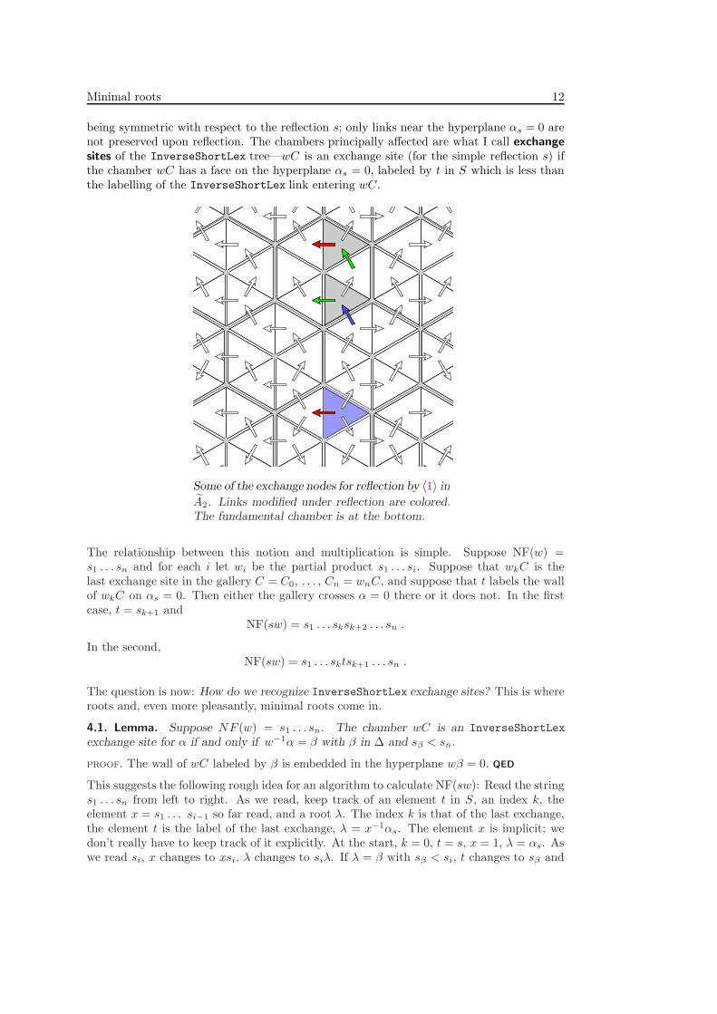
being symmetric with respect to the reflection s; only links near the hyperplane αs = 0 arenot preserved upon reflection. The chambers principally affected are what I call exchangesites of the InverseShortLex tree—wC is an exchange site (for the simple reflection s) ifthe chamber wC has a face on the hyperplane αs = 0, labeled by t in S which is less thanthe labelling of the InverseShortLex link entering wC.
Some of the exchange nodes for reflection by 〈1〉 in
A2. Links modified under reflection are colored.The fundamental chamber is at the bottom.
The relationship between this notion and multiplication is simple. Suppose NF(w) =s1 . . . sn and for each i let wi be the partial product s1 . . . si. Suppose that wkC is thelast exchange site in the gallery C = C0, . . . , Cn = wnC, and suppose that t labels the wallof wkC on αs = 0. Then either the gallery crosses α = 0 there or it does not. In the firstcase, t = sk+1 and
NF(sw) = s1 . . . sksk+2 . . . sn .
In the second,NF(sw) = s1 . . . sktsk+1 . . . sn .
The question is now: How do we recognize InverseShortLex exchange sites? This is whereroots and, even more pleasantly, minimal roots come in.
4.1. Lemma. Suppose NF (w) = s1 . . . sn. The chamber wC is an InverseShortLex
exchange site for α if and only if w−1α = β with β in ∆ and sβ < sn.
PROOF. The wall of wC labeled by β is embedded in the hyperplane wβ = 0. QED
This suggests the following rough idea for an algorithm to calculate NF(sw): Read the strings1 . . . sn from left to right. As we read, keep track of an element t in S, an index k, theelement x = s1 . . . si−1 so far read, and a root λ. The index k is that of the last exchange,the element t is the label of the last exchange, λ = x−1αs. The element x is implicit; wedon’t really have to keep track of it explicitly. At the start, k = 0, t = s, x = 1, λ = αs. Aswe read si, x changes to xsi, λ changes to siλ. If λ = β with sβ < si, t changes to sβ and
Minimal roots 13
k to i. When we are about to read si, sx = s1 . . . sktsk+1 . . . si−1. When we are throughscanning, we have the data determining the last exchange.
So far, minimal roots have not come into play. But in fact, in calculating the reflected rootsλ we only need to apply the minimal root reflection table. If λ is minimal and sλ = ⊖,then the chambers wi−1Ci−1 and Ci = wi−1siCi−1 lie on opposite sides of the hyperplaneα = 0, so we know we are looking at a deletion, and we need know no more. If sλ is minimaland sλ = ⊕ then we know the gallery has crossed a hyperplane λ = 0 which separates wCfrom α = 0. The exchange we last recorded will be the last we ever record, because thegallery cannot recross that hyperplane to reach αs = 0.
Pseudocode. The procedure has arguments s and the string s1 . . . sn representing w. Ituses variables
t: an element of S; initially si: in the range [0, n]; initially 0k: also in the range [0, n]; initially 0λ: an extended minimal root—either a minimal root or ⊕ or ⊖; initially αs
x: an element of W ; initially 1
BEGINNING OF LOOP. At this point x = s1 . . . si−1, sx = s1 . . . sktsk+1si−1, λ = x−1αs.
Read the next generator si. Then x becomes x = xsi. Set λ = siλ from the minimal rootreflection table.
If λ = β in ∆ with sβ < si, then set t = sβ , k = i.If λ = ⊖, this means k = i − 1 and si = t.
Set NF(sw) = s1 . . . si−1si+1 . . . sn and stop.If λ = ⊕, set NF(sw) = s1 . . . sktsk+1sk+2 . . . sn and stop.
Advance i to i + 1. If i > n, stop with NF(sw) = s1 . . . sktsk+1sk+2 . . . sn. Else loop.
We now know how to use the minimal root reflection table to multiply, and it remains tosee how to construct it.
5. A rough guide to constructing the minimal roots
A straightforward procedure to make a list of all minimal roots, along with a description ofhow reflections by the elements of S affect them, is not difficult to sketch.
The data associated to a minimal root λ, at least in this first approach, are to be:
• an array of coordinates;• its index (in the list of minimal roots);• a list of reflections sλ.
There are two natural choices of coordinates. Those I use in this note are the ones in theexpression of a root as a linear combination of the roots in ∆:
λ =∑
α∈∆
λαα .
The other reasonable choice is the array (λ •α), which du Cloux has discovered to be achoice somewhat more efficient in programming, if also more difficult to work with. Indicesare assigned in the order in which the minimal roots are first calculated; the roots in ∆are assigned the first |S| integers. Furthermore, in the preliminary version of the algorithmwe shall maintain a look-up table of some kind, enabling us to find a root’s data given itscoordinates, if it has already been encountered.
A minimal root is to be dealt with in two stages: (1) installing it and (2) finishing it. Inthe installation of a root
Minimal roots 14
⋄ its coordinate array is calculated;⋄ it is assigned an index;⋄ it is entered in the look-up table;⋄ a few reflections known at this time are registered;⋄ it is put on the waiting list of items to be finished.
The algorithm begins by installing the elementary roots α, which includes recording thereflections sαα = ⊖.
Items are taken off the waiting list in the order in which they are put on—the list is, inprogrammers’ terminology, a FIFO list (first in, first out) or queue. Roots are processed inorder of depth, so that if δ(λ) < δ(µ) the root λ is installed before µ.
When a root λ is to be finished, it is taken off the queue and all of the reflections sλ notalready known are found. At this moment, all roots with depth less than that of λ havebeen finished, so that in particular we have recorded all reflections µ = sλ ≺ λ. We mustcalculate the sλ not yet determined—we must decide whether sλ = λ, sλ is a minimal rootabove λ in the root graph, or sλ = ⊕. We can tell easily whether sλ = λ. Otherwise weknow that λ ≺ µ = sλ. There are three possibilities: (a) The root µ is minimal, and wehave already installed it. It will be registered in our look-up table. We just add to therecord that sλ = µ and sµ = λ. (b) The root µ is not minimal. The criterion is that sα
and sµ generate an infinite group, or equivalently that λ •αs ≤ −1. We can tell this whenwe calculate µ. In this case we set sλ = ⊕. (c) Otherwise −1 < λ •αs < 0 and the root µ isa new minimal root not yet installed. We do so by assigning it an index, putting it in thelook-up table, recording the reflection sλ = µ, and putting µ in the process queue. After allsλ have been found, we go on to the next root in the queue, as long as there is somethingthere.
There are a couple of important simplifications that can be made to this procedure.
Eliminating the look-up table. Maintaining the look-up table is somewhat cumbersome.It was du Cloux who first observed that one can dispense with it. The only place where itis used is in case (a) above, where we are recording that sαλ = µ with µ already installed,and there is a better way to deal with this.
A root in the linear span of a pair of roots in ∆ is called dihedral. Suppose for the momentthat s and t are distinct elements of S. A root λ is a linear combination of αs and αt if andonly if the orbit of λ with respect to the subgroup Ws,t generated by s and t contains oneof αs or αt. Installing the dihedral roots is a simple task, and can (and should) be doneindependently of all other installations, as we shall see later.
To any Coxeter system (W, S) is associated a partial ordering, sometimes called the weakright Bruhat order—the nodes are elements of W and there is an oriented edge w → wslabeled by s if ℓ(ws) = ℓ(w) + 1. The identity is the unique minimal node, and if thegroup is finite the unique highest node is the element of greatest length in W . Finite pathsin this graph starting at 1 correspond precisely to reduced expressions of elements of Wassembled from the labels of the edges followed. For a finite dihedral group Ws,t this graphis particularly simple—there are two paths st . . . and ts . . . of length m from 1 to the longestelement ws,t corresponding to the two reduced expressions for ws,t assured by the Coxeterrelation (st)m = 1. The Bruhat order is intimately related to the geometry of roots andchambers.
The first of the following two lemmas is well known:
5.1. Lemma. For T ⊆ S, every element of the subgroup WT permutes all the positive rootsthat are not in the linear span of the αs with s in T .
Minimal roots 15
The next one has for me a mildly paradoxical flavour.
5.2. Lemma. Suppose s, t to be a pair of elements of S, µ to be a positive root not in thespan of αs and αt. Assume that αs •µ > 0 and αt •µ > 0. Then Ws,t is finite, and themap w 7→ wµ is a bijection between Ws,t and Ws,tµ inducing an isomorphism of the weakBruhat order with inverted precedence in the root graph.
That is to say that ℓ(w) < ℓ(sw) for s in T if and only if swµ ≺ wµ. Equivalently, if ν is theroot of least depth in the Ws,t-orbit then w 7→ wν is a order-preserving bijection betweenWs,t and Ws,tµ.
PROOF. Let T = {s, t}. By assumption, all roots in the WT -orbit of µ are positive roots.The region αs • v > 0, αt • v > 0 is a fundamental domain for Ws,t. If v is any vector in thisregion, w in W , then ℓ(xw) = ℓ(w) + 1 for x in T if and only if wv •αx > 0. If ν is a rootin the WT -orbit of least depth then αx • ν < 0 for x in T . Proposition 1.1 implies that WT
is finite, and the rest follows easily. QED
How can this be applied in our algorithm to find all minimal roots? Suppose we are in theprocess of installing a minimal root µ. We may assume it not to be dihedral, because wecan deal separately with all the dihedral roots in a particularly simple fashion. So we arelooking at µ = sλ with λ ≺ µ. Two questions arise: (a) For t in S, how do we tell whethertµ ≺ µ or not? (b) If so, then tµ has already been finished. How do we identify it?
If Ws,t is infinite, then by Proposition 5.2 the problem doesn’t occur. Otherwise, let ws,t
be the longest element in Ws,t. Calculate the element ν of least depth in Ws,tµ, by findingalternately tλ, stλ, etc. until the chain starts to ascend in depth. The Lemma tells usthat tµ ≺ µ if and only if the difference in depth between µ and ν is exactly ms,t. Inthese circumstances the element tµ will then be (tws,t)ν, which can be calculated from thereflection tables of elements of depth less than λ. In other words, as soon as µ is installedwe can calculate all the descents tµ ≺ µ—without doing any new calculations!
In the algorithm above we can therefore eliminate the look-up table. The procedure sketchedabove requires, however, that we know whether the reflection of a root has less depth ornot, so we add to the data of a root λ its descent set, the set of s with sλ ≺ λ. When weinstall a root, before we put it in the queue, we calculate all of its descents. (An alternativewould be to store the depth of a root as part of its data.)
As has already been mentioned, because the result above is applicable only to roots notin the orbit of αs and αt under Ws,t, all the dihedral roots have to be handled somewhatspecially—they should all be installed immediately after the roots in ∆, and those of depthgreater than 2 have to be fed into the queue at the right moment.
One huge benefit of this technique is that it requires arithmetic only to decide whethersαλ = λ or not.
Noting inherited locks. The following was observed by Brink and Howlett, and used as animportant part of their proof that the set of minimal roots is finite:
5.3. Proposition. If sλ = ⊕ and λ ≺ µ then sµ = ⊕ as well.
PROOF. Let α = αs. If λ is a minimal root, the according to the Minimality Criterion sλ = ⊕if and only if λ •αs ≤ −1.
For β in ∆, λ any root
sβλ •α =(λ − 2(λ •β)β
)•α = (λ • α) − 2(λ •β)(β •α)
Minimal roots 16
which means that for β 6= α the dot product λ •α does not increase under reflection by β,as long as λ ≺ sβλ and therefore λ •β < 0. Therefore once we have calculated that sλ = ⊕this remains true for all minimal µ with λ ≺ µ. QED
This result is the crucial part of the proof by Brink and Howlett that the number of minimalroots is finite. By Konig’s Lemma, if there an infinite number, then in the part of the rootgraph composed of minimal roots there would exist an infinite chain. For each λ in thischain, let ¶λ be the subset of α in ∆ with sαλ = ⊕. According to the Proposition, the setPα is non-decreasing, so in an infinite chain of minimal roots it must be stationary withnon-trivial complement. Let P be the intersection, and choose λ be such that Pλ = P forλ � µ in the chain. Beyond λ, reflection by α in P never occurs, so µα for all λ � µ.Furthermore, the set of possible values of µ •α for α in the complement of P lies in (−1, 1),and must be finite. Therefore there must exist µ1 and µ2 such that (a) µ1,α = µ2,α for α inP and (b) µ1 •α = µ2 •α for α in its complement. Lemma 2.7 of of B & H then implies thatµ1 •µ2 = 1, which means that one of them dominates the other, which is a contradiction.
I call an s with sλ = ⊕ a lock on λ at s. This Proposition tells us that locks are inheritedas we go up the root graph and these inherited locks, like descents, can be immediatelyrecorded upon installation.
In the simplest cases—when none of the Coxeter matrix entries ms,t are greater than 3—there is probably no better algorithm than the one sketched above, but incorporating thesimple modifications concerning descents and locks. In fact, one can even apply it when theCoxeter group is the Weyl group of an integral root system, taking into account a differentrealization of the group. In this case, all doubled dot products 2 (λ •α) will be integers.When λ ≺ sαλ this doubled dot-product will be a negative integer, and if it is anythingother than −1 the root sλ will no longer be minimal. What could be simpler?
If there are entries ms,t > 3 and we are using the standard realization, however, we haveto deal with non-rational cyclotomic arithmetic. The algorithm described still works, atleast in principle, although there are a few annoyances that arise. All dot products in therange (−1, 0) will be of the form cos
(πk/ms,t
)for k < ms,t/2. So in order to tell whether
sλ dominates αs we just have to compare the dot product λ •αs to numbers in this finiteset. There is one potentially nasty problem, however. All we can assert a priori about thecoordinates of λ is that they will be in the real cyclotomic field generated by cos(2π/M),where M is the lowest common multiple of the numbers 2ms,t. The amount of work involvedwould seem to grow disturbingly as M grows. I call this the problem of mixed cyclotomy.
There is one problem related to this that I might have mentioned earlier. It is difficult totell whether real elements of a cyclotomic field are positive or not if they are representedas floating point real numbers. Thus one has to be careful. There are some obvious waysto get around this—for example, working very high precision—but they are inefficient. Soat first sight it looks like we are faced with a dilemma. We want to work with exactcyclotomic arithmetic to avoid rounding errors, but will then have trouble detecting thesign of numbers and will also face intricate calculations. Brink’s thesis tells us that boththese apparent difficulties are spurious. In the next section I’ll digress somewhat to explainhow the technique introduced here can be used in another computation, but in the one afterthat I’ll follow Brink in examining more carefully the coefficients of minimal roots.
Minimal roots 17
6. Integral root systems
I’ll explain in this section how the technique explained just now to avoid table look-up inconstructing minimal roots of a Coxeter group can also be used to construct the root graphfor the system of real roots of a Kac-Moody algebra, at least as much of it as is practical.
Let ∆ be a basis of a free Z-module L of finite rank, and suppose that to each α in ∆ isassociated a vector α∨ in the dual lattice L, such that (a) 〈α, α∨〉 = 2; (b) 〈α, β∨〉 = 0 if andonly if 〈β, α∨〉 = 0; (c) 〈α, β∨〉 ≤ 0 for α 6= β. Then for each α the linear transformation
sα∨ : λ 7−→ λ − 〈λ, α∨〉α
is a reflection. Letnα,β = 〈α, β∨〉〈β, α∨〉 .
It is non-negative. The group W generated by these reflections is a Coxeter group with
mα,β =
2 if nα,β = 03 if nα,β = 14 if nα,β = 26 if nα,β = 3∞ if nα,β ≥ 4
The transforms of elements of ∆ by W are called the roots of the system, and they are thereal roots of the Kac-Moody algebra determined by the Cartan matrix (〈α, β∨〉). Theseroots are in bijection with those constructed earlier from the standard Cartan matrix(−2 cosπ/mα,β), but the corresponding linear representations of W won’t be isomorphicunless the matrix C = (〈α, β∨〉) is symmetrizable—that is to say DC is symmetric for somediagonal matrix D with positive diagonal entries. This happens rarely.
As earlier, the root graph has as its nodes the roots λ, and an oriented edge λ → sαλ if〈λ, α∨〉 < 0 and a loop from λ to itself labelled by α if sαλ = λ or equivalently 〈λ, α∨〉 = 0.This root graph is isomorphic to the one constructed from the standard Cartan matrix,but in constructing it one might want to keep track of explicit data such as the explicitexpression λ =
∑λαα, so there is some point to describing its construction directly in
terms of these coefficients.
The goal now is to find all roots up to a certain depth d. The processes of installationand finishing are pretty much the same, except that we have to include as part of the dataattached to a root its depth as well as its index of coefficients, so we can avoid installingroots of depth > d. The important point is that we can use the same trick described beforein order to tell for a new non-dihedral root µ = sλ with tλ ≺ λ whether tµ < µ or not bycalculating tλ, stλ, etc. until we get to a root of minimal depth in the Ws,t-orbit of λ.
Incidentally, as the diagram for the root graph in §3 shows, root graphs exhibit an interestingrepetitive structure. Howlett tells me that he has shown that it is always the set of pathsthrough a finite automaton. One can in effect describe the whole root graph in finite,relatively simple terms.
Minimal roots 18
7. Root coefficients
We want to know something about what possible values can occur for the coefficients ofroots and, especially, minimal roots. Roots are produced by a sequence of reflections fromthe basic roots in ∆. As is the case in many algorithmic processes, although we understandeach single step—here, reflection—quite well, the overall development is not so clear.
We begin by looking at dihedral roots.
Suppose S to possess exactly two elements s and t, corresponding to roots α and β. Letm = ms,t. What are all the positive roots of the system? Let
z = ζ2m = e2πi/2m = eπi/m = cos(π/m) + i sin(π/m)
so that−2 α •β = 2 cos(π/m) = (z + z−1) = (say) c
andsλ = λ − 2(λ •α)α
2 (pα + qβ) • α = 2p − cq
s(pα + qβ) =[− p + cq
]α + qβ
tλ = λ − 2(λ •β)β
2 (pα + qβ) •β = 2q − cp
t(pα + qβ) = pα +[− q + cp
]β .
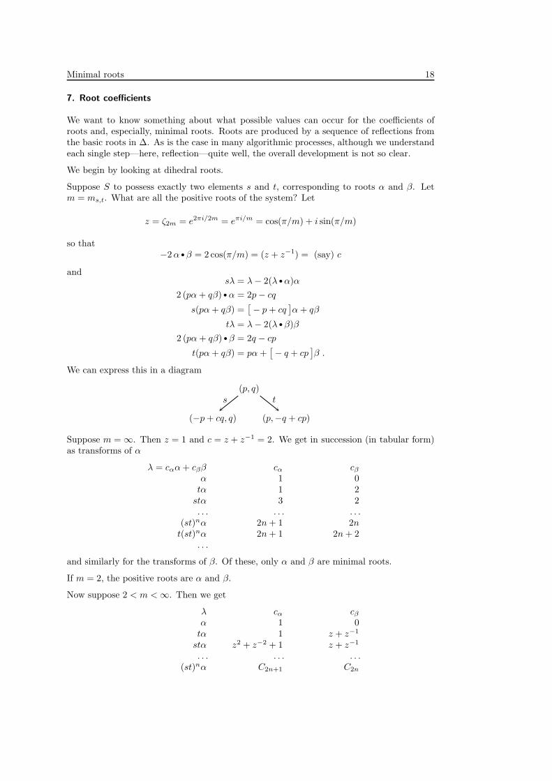
We can express this in a diagram
(p, q)
(−p + cq, q) (p,−q + cp)
s t
Suppose m = ∞. Then z = 1 and c = z + z−1 = 2. We get in succession (in tabular form)as transforms of α
λ = cαα + cββ cα cβ
α 1 0tα 1 2
stα 3 2. . . . . . . . .
(st)nα 2n + 1 2nt(st)nα 2n + 1 2n + 2
. . .
and similarly for the transforms of β. Of these, only α and β are minimal roots.
If m = 2, the positive roots are α and β.
Now suppose 2 < m < ∞. Then we get
λ cα cβ
α 1 0tα 1 z + z−1
stα z2 + z−2 + 1 z + z−1
. . . . . . . . .(st)nα C2n+1 C2n
Minimal roots 19
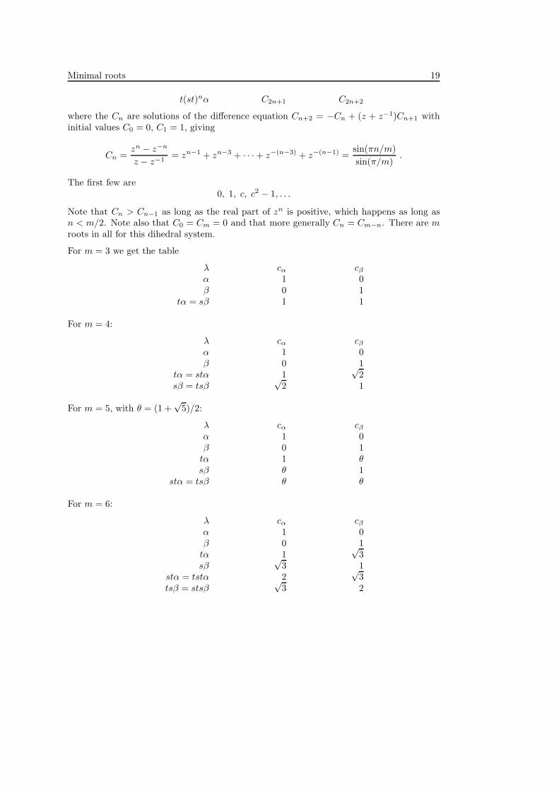
t(st)nα C2n+1 C2n+2
where the Cn are solutions of the difference equation Cn+2 = −Cn + (z + z−1)Cn+1 withinitial values C0 = 0, C1 = 1, giving
Cn =zn − z−n
z − z−1= zn−1 + zn−3 + · · · + z−(n−3) + z−(n−1) =
sin(πn/m)
sin(π/m).
The first few are0, 1, c, c2 − 1, . . .
Note that Cn > Cn−1 as long as the real part of zn is positive, which happens as long asn < m/2. Note also that C0 = Cm = 0 and that more generally Cn = Cm−n. There are mroots in all for this dihedral system.
For m = 3 we get the table
λ cα cβ
α 1 0β 0 1
tα = sβ 1 1
For m = 4:
λ cα cβ
α 1 0β 0 1
tα = stα 1√
2sβ = tsβ
√2 1
For m = 5, with θ = (1 +√
5)/2:
λ cα cβ
α 1 0β 0 1
tα 1 θsβ θ 1
stα = tsβ θ θ
For m = 6:
λ cα cβ
α 1 0β 0 1
tα 1√
3sβ
√3 1
stα = tstα 2√
3tsβ = stsβ
√3 2
Minimal roots 20
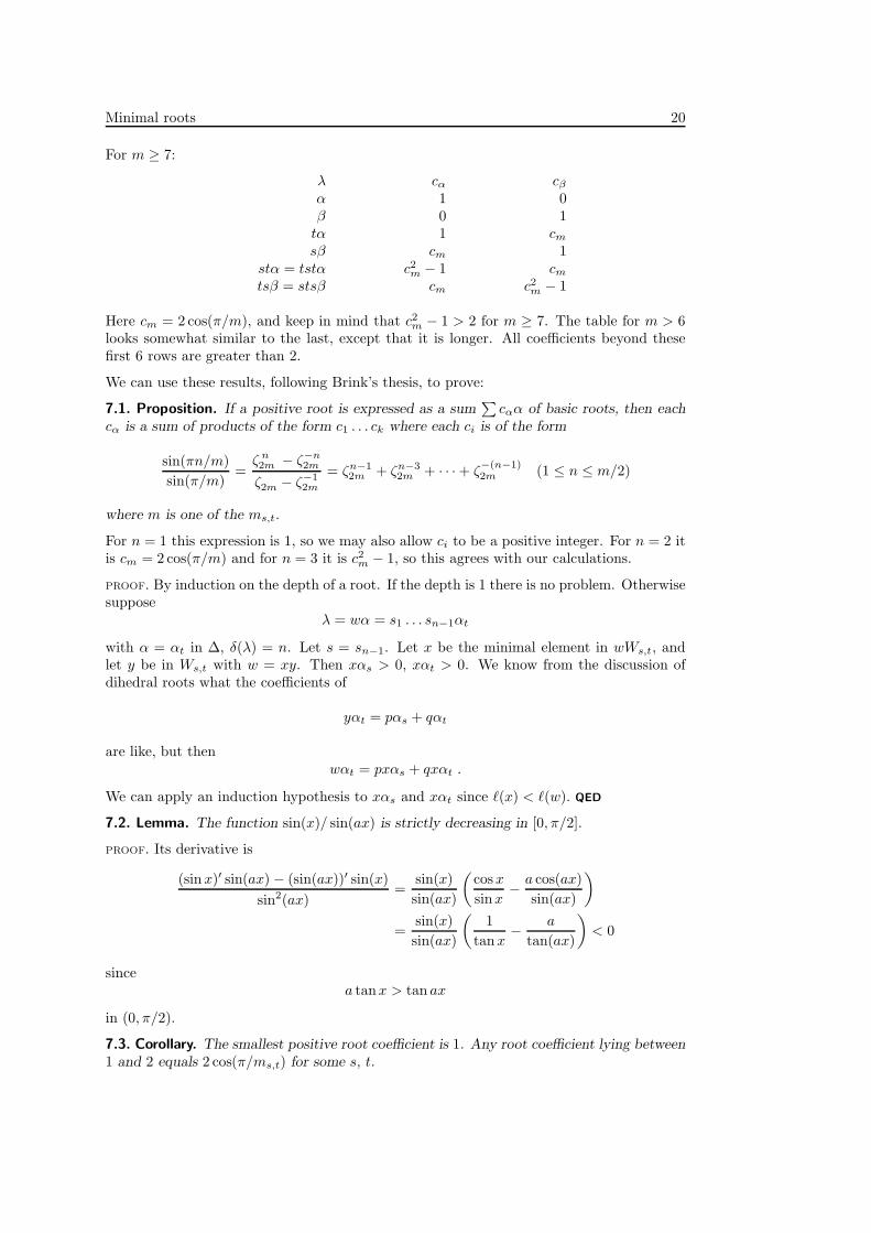
For m ≥ 7:
λ cα cβ
α 1 0β 0 1
tα 1 cm
sβ cm 1stα = tstα c2
m − 1 cm
tsβ = stsβ cm c2m − 1
Here cm = 2 cos(π/m), and keep in mind that c2m − 1 > 2 for m ≥ 7. The table for m > 6
looks somewhat similar to the last, except that it is longer. All coefficients beyond thesefirst 6 rows are greater than 2.
We can use these results, following Brink’s thesis, to prove:
7.1. Proposition. If a positive root is expressed as a sum∑
cαα of basic roots, then eachcα is a sum of products of the form c1 . . . ck where each ci is of the form
sin(πn/m)
sin(π/m)=
ζ n2m − ζ−n
2m
ζ2m − ζ−12m
= ζn−12m + ζn−3
2m + · · · + ζ−(n−1)2m (1 ≤ n ≤ m/2)
where m is one of the ms,t.
For n = 1 this expression is 1, so we may also allow ci to be a positive integer. For n = 2 itis cm = 2 cos(π/m) and for n = 3 it is c2
m − 1, so this agrees with our calculations.
PROOF. By induction on the depth of a root. If the depth is 1 there is no problem. Otherwisesuppose
λ = wα = s1 . . . sn−1αt
with α = αt in ∆, δ(λ) = n. Let s = sn−1. Let x be the minimal element in wWs,t, andlet y be in Ws,t with w = xy. Then xαs > 0, xαt > 0. We know from the discussion ofdihedral roots what the coefficients of
yαt = pαs + qαt
are like, but thenwαt = pxαs + qxαt .
We can apply an induction hypothesis to xαs and xαt since ℓ(x) < ℓ(w). QED
7.2. Lemma. The function sin(x)/ sin(ax) is strictly decreasing in [0, π/2].
PROOF. Its derivative is
(sin x)′ sin(ax) − (sin(ax))′ sin(x)
sin2(ax)=
sin(x)
sin(ax)
(cosx
sinx− a cos(ax)
sin(ax)
)
=sin(x)
sin(ax)
(1
tanx− a
tan(ax)
)< 0
sincea tanx > tan ax
in (0, π/2).
7.3. Corollary. The smallest positive root coefficient is 1. Any root coefficient lying between1 and 2 equals 2 cos(π/ms,t) for some s, t.
Minimal roots 21
PROOF. Because of the Lemma, the minimum value of sin(x)/ sin(ax) in [0, π/2] is 1/ sin(πa/2).If a = 1/n with n ≥ 3, this lies at or above 2. Therefore all possible values of sin(x)/ sin(x/n)for 0 ≤ x ≤ π/2 in the range (1, 2) are with n = 2, when this is just 2 cos(x/2). The minimumvalue achieved is 2 cos(π/4) =
√2. Any root coefficient will be a sum of terms
C = c1 . . . ck
where k ≥ 1 and each ci will be either a positive integer or one of the constants in theProposition. If C itself is not 1 then we may assume that each ci > 1. The smallest possiblevalue for one of these constants is 1, and the second smallest possibility is
√2. So if C is
less than 2 then k = 1, and is an integer only if it is 1. QED
7.4. Corollary. The smallest possible coefficient of a positive root, other than 1, is√
2.
8. The support of minimal roots
One of the principal results of Brink’s thesis is that the apparent difficulties concerningmixed cyclotomy in the determination of the minimal roots do not actually arise—we neednever do arithmetic in cyclotomic fields other than the ones generated by some ms,t-th rootsof unity.
In order to see why this is so, we have to look carefully at how roots are calculated.
A root∑
λαα may be considered as a function on the Coxeter graph: s 7→ λαs. The support
of a root λ =∑
λαα is its support as a function—the set of s where λαs6= 0. One of Brink’s
nice ideas is to track the computation of roots by looking at their support. All roots areconstructed by applying some element of W to a basic root, and we are going to constructthem by ascending the root graph.
Upon reflection by s, only the coefficient λα changes, and to
−λα +∑
λβ 6=0, α∼β
[−2 α •β] λβ .
According to Corollary 3.4, the support of a root cannot decrease as we go up the rootgraph. Under what circumstances it is extended? In going up the root graph from λ to sλ,the support of λ is extended if s is not already in its support. If s is not connected to thatsupport in the Coxeter graph, then sλ = λ. This process gives a new root only when s islinked to the support of λ. Therefore:
8.1. Proposition. The support of any root is connected.
Suppose we apply a reflection s to a positive root λ whose support does not contain s. Theformula for reflection is
sαλ = λ − 2 (λ •α)α
whereα •λ =
∑
β
λβ(α •β) = λα +∑
λβ 6=0, α∼β
λβ [α •β]
if λ =∑
λαα. How does the support of a root get extended? If λ is a minimal root withλαs
= 0, then sλ will also be a minimal root if and only if −1 < λ •α, or equivalently
∑
λβ 6=0, β∼α
[−2 α •β] λβ < 2 .
Minimal roots 22
But λβ ≥ 1 and also −2 α •β ≥ 1. The condition for minimality cannot hold here unlessthere is just one β = αt in the sum. Furthermore, in that case the condition above amountsto requiring that
[−2 α •β] λβ < 2 .
The first term is either 1 or ≥√
2, as is the coefficient λβ . All in all:
8.2. Proposition. Suppose λ to be a minimal root, s an element of S not in the support Θof λ. If sλ is again minimal then there must be just a single link from s to Θ, say to t, andone of these holds:
(a) ms,t = 3 and λαt< 2;
(b) 3 < ms,t < ∞ and λαt= 1.
We can summarize this in a mnemonic diagram:
• 1 0 7−→ 1 1
• c 0 7−→ c c (1 < c < 2)
• 1m
0 7−→ 1m
c(c = 2 cos(π/m)
)
where means an edge of multiplicity 3 and one of higher multiplicity.
8.3. Corollary. The support of a minimal root is a tree containing no links of infinite degree.
9. Composition and decomposition
The most important of Brink’s ideas is to understand that minimal roots can be assembledin a simple way from relatively simple ones.
The trick is to focus on the coefficients of a minimal root that are equal to the minimumpossible value 1. This leads to a remarkable view of the structure of a minimal root, whichI’ll explain in the rest of this section. Suppose λ to be a minimal root with λα = 1. Letα = αs. We know that λ has been built up from a chain of minimal root predecessors
λ1 ≺ . . . ≺ λn = λ .
Some one of these, say µ = λk, will be the first to have a non-zero coefficient of α, andthat coefficient must be 1, since by Corollary 3.5 coefficients can only grow as we move upthe root graph. Unless µ = λ1 = α, the root µ must have been constructed by extensionfrom a root λk−1 whose support did not contain s, and the earlier Proposition tells us thatµ = sλk−1, where s is linked to the support of λk−1 at a single node t by a simple link inthe Coxeter graph, and λk−1,αt
= λk,αt= 1. We have λ = wµ where w is a product of
generators other than s.
Since the support Θ of λ is a tree, the complement of s in Θ is the disjoint union of exactlyas many components Θ•
i as there are edges in Θ linked to s, say ℓ. Reflections correspondingto nodes in different components will commute. Hence we can write λ = w1 . . . wℓµ whereeach wi is in WΘ•
i. All the wi commute, so we can write the product in any order. Each of
the λi = wiα is itself a root with support in Θi = Θ•i ∪ {s}, minimal because it will be a
predecessor of λ in the root graph. We have therefore proven:
9.1. Proposition. Let λ be a minimal root with λαs= 1. Let Θ be the support of λ, the
Θ•i the connected components of Θ\{s}, Θi = Θ•
i ∪ {s}. The restriction λi of λ to Θi isalso a minimal root.
This is called the decomposition of λ at s. Conversely:
Minimal roots 23
9.2. Proposition. Let Θ be a subset of S, s an element of Θ, the Θ•i the components of
Θ\{s}, Θi = Θ•i ∪ {s}. If for each i the minimal root λi has support on Θi with coefficient
1 at αs, then the vector λ with support Θ whose restriction to each Θi agrees with λi is aminimal root.
This is called composition or amalgamation at s.
PROOF. More difficult than the previous result. It follows from this result of Brink’s:
9.3. Lemma. If λ is any positive root with coefficient 1 at α = αs, then λ = wα, where wis a product of t 6= s in S.
PROOF. Induction on the depth of λ. Trivial if λ = α. It remains to be shown that if δ(λ) > 1and λα = 1 then we can find s such that sλ ≺ λ and sλ also has coefficient 1 at α. Thereexists at any rate some s with sλ ≺ λ. If this does not have coefficient 1 at α, then—aswe have seen above—sλ has coefficient 0 at α; α has exactly one link to the support of sλ,say to β; and the coefficient of sλ at β is equal to 1. By induction, sλ = wβ where w is aproduct of t equal neither to s nor sβ . But then
λ = swβ = wsα . QED
These results have a natural generalization, allowing us to compose and decompose atcollections of more than one node. The unit support of λ is the set of α with λα = 1.Suppose λ to be a minimal root, Θ its support, T ⊂ Θ its unit support. We know thatΘ is a connected tree. The complement Θ\T can be expressed as the disjoint union of itsconnected components Θ•
i . For each of these, let Θi be its union with the elements of Tattached to it. Each set Θi will then be connected, and no point of T will be in its interior.The set T will contain in addition some pairs of nodes of the Coxeter graph connected bylinks in it; let these be counted as additional sets Θi (but with empty interiors). Finally,there is one exceptional case where Θ has just one element, which is Θ1.
9.4. Lemma. The set Θ is the union of the Θi, which overlap only in points of T .
PROOF. We may suppose Θ to have more than one element in it. Suppose given t in Θ. If itis not in T , it belongs to a unique Θ•
i . Otherwise, it will be in T . If it is connected in theCoxeter diagram to one of the Θ•
i , it will be in Θi. Finally, we have the situation where theonly elements of Θ it is linked to are in T . Each of the pairs forming such a link will be oneof the Θi. QED
If T is any subset of S, a subset Θ is called T-connected if connected and none of its interiorpoints belong to T . Each of the Θi defined above are T -connected, and are called the T-components of Θ. Following Brink, I call a minimal root indecomposable if its supportis T -connected, or in other words if its unit support is contained in the boundary of itssupport.
9.5. Lemma. (Brink) (Decomposition) The restriction of a minimal root to any of theT -components of its support is again a minimal root.
PROOF. This follows by induction from the earlier decomposition. QED
As does this:
9.6. Proposition. (Brink) (Composition) Let Θ be any connected, simply connected subsetof S, T an arbitrary subset of Θ, Θi its T -components. If λi is for each i a minimal rootwith support Θi and unit support T ∩Θi, then the vector λ with support Θ whose restrictionto each Θi is λi will be a minimal root.
Minimal roots 24
This reduces the calculation of minimal roots to the calculation of indecomposable ones,together with a bit of accounting—i.e. joining indecomposable ones together in their unitsupports. Finding the reflection table turns out not to be much more difficult.
It is useful to restate the criterion here:
• (Indecomposability criterion) Suppose λ to be a minimal root with support Θ. Thenλ is indecomposable if and only if either (a) Θ = {s} or (b) every node of Θ in theunit support of λ is connected to exactly one other node in Θ.
10. Constructing the indecomposable minimal roots
So now the question we have to deal with is, How are indecomposable roots to be found?They are obtained by reflection from predecessors in the root graph. The predecessors mayor may not be indecomposable. What can we say about the process of forming them? Ittakes place in simple steps, so we just have to understand the simple steps, going up the rootgraph one edge at a time. The most important question is this: If λ is an indecomposableroot and µ = sλ ≺ λ, what can we say about µ? Let Θ be the support of λ, and let α = αs.There are several possibilities.
• Suppose that s is a boundary point of Θ with λα = 1. Then according to Proposition8.2 the root λ is obtained from µ by extension along a simple edge from a unit nodet of µ. This is also a unit node of λ. By the indecomposability criterion this canhappen only if µ = αt.
• Suppose that s is in the boundary of Θ but that λα > 1. Let t be the uniquenode that s is connected to. There are two possibilities: (a) the support of µ is onenode less that of λ or (b) it is the same. Case (a) also breaks down by Proposition8.2 into two possibilities: (i) the node t is in the unit support of µ, hence of λ.Since λ is indecomposable µ = αt, the link from s to t has multiplicity m > 3, andλα = 2 cos(π/m). (ii) The link from s to t is simple, and λα = λαt
. In case (b) wecan deduce at least that µ is also an indecomposable root.
• Suppose α lies in the interior of Θ. Then by Proposition 8.1 it cannot happen thatµα = 0. Suppose µα > 1. Then µ is also indecomposable.
• Finally, suppose α lies in the interior of Θ but µα = 1. The support of µ is also Θ, soµ cannot be indecomposable. It will be the composite of two or more indecomposableroots µi adjoined to each other at α.
Running this backwards:
10.1. Proposition. Every indecomposable root is constructed through a sequence of reflec-tions µ ≺ sµ = λ falling into one of three possible types:
(1) extension, where the support of µ is less than that of λ;(2) promotion, where µ is indecomposable and has the same support as λ;(3) fusion, where µ is the composite of indecomposable roots µi each with αs in its unit
support.
We have already investigated extension in detail, but here I point out that if it is going tolead to an indecomposable root it has to be the process
• c 0 7−→ c c (1 < c < 2) .
There is nothing particularly subtle about promotion. In the next section we look at fusion,about which we can say something interesting.
Minimal roots 25
11. Reflecting at junctions
This section is unavoidably technical, but also crucial towards understanding how the even-tual program will work. Let me try to summarize how things go, before starting to plow.
Suppose we are given a minimal root λ with support Θ as well as an elementary reflections. The basic question throughout this paper is whether sλ is again a minimal root. Letα = αs. There are three cases:
(a) If s is in the support of λ, and the coefficient λα > 1, we are looking at the processof promotion. This node will occur in the interior of one of the Brink components of Θ,so we are looking at promotion of this component. We might have to do some cyclotomicarithmetic to carry it out, but the structures we are looking at are not going to changemuch—at most we have to change a single root coefficient.
(b) The generator s is not in Θ. If sλ is again indecomposable, s must be linked to Θ by asingle edge with certain restrictions we have already mentioned.
(c) The node s is in the support of λ, but the coefficient λα = 1. If this node is on theboundary of Θ, we are again looking at promotion, and again of a single component of Θ.Otherwise, this node has links to at least two nodes of Θ. This is the case I have calledfusion, and it is the case we are going to examine in this section. The main consequence ofthe investigation is that mixed cyclotomy does not occur, which is extremely important toknow when programming. Also, the code for fusion follows the treatment below very closely.
Suppose Θ to be a connected and simply connected subset of S, s an interior node of Θ,the Θi the connected components of Θ\{s}. Suppose that λ is a minimal root with supportΘ and λα = 1 where α = αs. Let λi be the restriction of λ to Θi, and assume the λi areindecomposable. In this section we’ll answer the following question:
• In these circumstances, when is sλ a minimal root?
Each of the Θi contains a unique node ti linked to s. Let βi = αti. The sort of things we
have to answer are: How many components Θi are allowed? What are the possible valuesfor λβi
?
The inner product λ •α is
1 −∑
λβi|α •βi| .
Recall that λβi≥ 1, |α •βi| ≥ 1/2. When the junction has more than 3 roots joining at it,
this dot-product is ≤ −1, and sλ will not be minimal.
11.1. Proposition. If Θ\{s} has more than 3 components, sλ = ⊕.
We may now assume there to be 2 or 3 links at α.
11.2. Lemma. Suppose c = 2 cos(π/ms,t). The links c 1 and 1 1 cannot occur inany root.
This introduces notation I hope to be self-explanatory. What I mean by this is that if λis a root then there do not exist neighbouring nodes s and t in the Coxeter graph with (1)ms,t = 3, λαs
= 1, 1 < λα1< 2; or (2) ms,t > 3, λαs
= 1, λα1= 1.
PROOF. Lemma 9.3 implies that 1 1 cannot occur, and then implies that if c 1occurs, so does 1 1. QED
We now consider the possibilities for fusion.
Minimal roots 26
Fusion from two links
The three a priori local possibilities for λ are (with s in the middle)
(2.a) λx 1 λy
(2.b) λx 1 λy
(2.c) λx 1 λy
with λ∗.
Case (2.c) We can eliminate one of these immediately.
11.3. Proposition. In the case (2.c) sλ = ⊕.
PROOF. The inner product λ •α is 1 − cxλx/2 − cyλy/2. We know that each c∗ is at least√2, and we know by the previous Lemma that λ∗ ≥
√2 as well. Thus the dot product is
−1 or less. QED
Case (2.a) The diagram is λx 1 λy.
In this case, the condition that sλ be minimal is that 1−λx/2−λy/2 > −1, or λx +λy < 4.The case λ∗ = c is excluded by the previous Lemma, so either λ∗ = 1 or λ∗ ≥ 2. It is notpossible for both λ∗ to be ≥ 2, so one at least must be 1, say λy = 1.
We can do better: the inner product must be − cos(πk/m) for k ≤ m/2. This gives us:
m = 3. The inner product is 0, with
• 1 1 1 7−→ 1 1 1
(which does not produce a new indecomposable root) or −1/2 with
• 2 1 1 7−→ 2 2 1 .
m = 4. We must have 1/2 − λx/2 = −√
2/2 or λx = 1 +√
2/2. Impossible.
m = 5. 1 − λx = −c or 1 − c, λx = 1 + c or λ = c. The second is impossible, alas. So theonly possibility is
• (1+c) 1 1 7−→ (1+c) (1+c) 1 .
m ≥ 6. Nothing possible.
Case (2.b) Here the diagram isλx 1 λy ,
and the condition is
1 − λx/2 − (c/2)λy > −1, λx + cλy < 4 .
m = 4. Only possibility is
• 1 1√
2 7−→ 1 2√
2 .
Minimal roots 27
m = 5. Only possibility is
• 1 1 c 7−→ 1 (1+c) c .
We can nicely summarize the results:
11.4. Proposition. If λ is the composition of two indecomposable roots at s, then sλ = ⊕unless one of the two components is 1 1, and in that case we are looking at one of thereflections expressed locally as
1 1 2 7−→ 1 2 2
1 14 √
2 7−→ 1 24 √
21 1 (1 + c) 7−→ 1 (1 + c) (1 + c)
1 15
c 7−→ 1 (1 + c)5
c
Note that in all these cases we start with λ a composition of two indecomposable roots, oneof which is just 1 1. So it is trivial to reconstruct the reflection even when this is allembedded in a generic root.
Fusion from three links
Assume the product of the reflection to be an indecomposable root. The conditions areλx + λy + λz < 4 if all links are simple, or λx + λy + cmλz < 4 if one has degree m > 3.More of degree m > 3 cannot occur by simple calculation. If m > 3 then c ≥
√2 so the
second sum is at least 4, and cannot occur.
As for the first, we cannot have any λ∗ ≥ 2, so each can only be 1 or c. But the link c 1cannot occur.
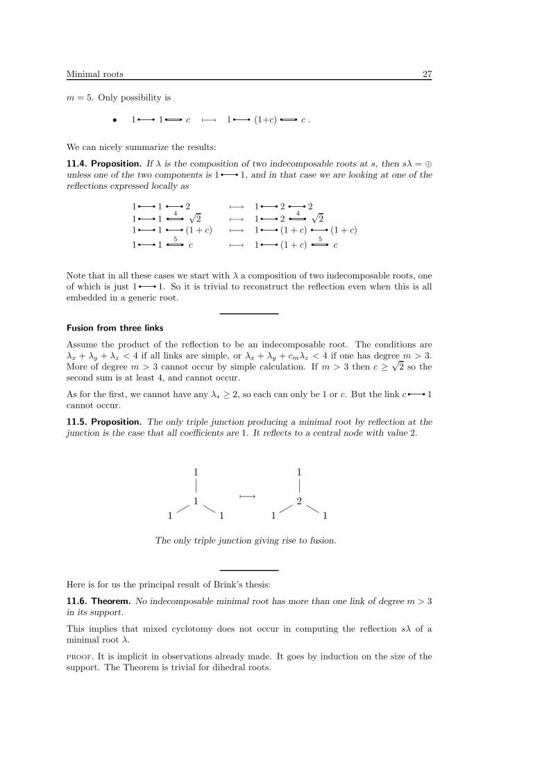
11.5. Proposition. The only triple junction producing a minimal root by reflection at thejunction is the case that all coefficients are 1. It reflects to a central node with value 2.
1
1
11
7−→2
1
11
The only triple junction giving rise to fusion.
Here is for us the principal result of Brink’s thesis:
11.6. Theorem. No indecomposable minimal root has more than one link of degree m > 3in its support.
This implies that mixed cyclotomy does not occur in computing the reflection sλ of aminimal root λ.
PROOF. It is implicit in observations already made. It goes by induction on the size of thesupport. The Theorem is trivial for dihedral roots.
Minimal roots 28
Suppose it to be true for all roots of size < n, and suppose we are looking at an indecom-posable root of size n. It arose in one of these ways:
• Extension from an indecomposable root. If the number of multiple links is to rise, then wemust have extended by a multiple root. But by Proposition 8.2 any extension by a multiplelink is decomposable.
• Promotion. The support is not extended.
• Fusion of two links. In this case, according to Proposition 9.1 one of the roots being fusedis a simple dihedral root, so there is no problem here, either.
• Fusion of three links. According to Proposition 9.2 the roots being fused are all simpledihedral roots. QED
Brink’s thesis at this point goes on to build a rather explicit description of all possibleindecomposable roots whose support is a given Coxeter graph. It is probably a poor idea totry to use these lists in a computer program, since it is easy enough to use basic propertiesof indecomposable roots to build these lists automatically.
There are a few important consequences of what we have seen so far that are not quiteobvious. Keep in mind that the qualities of a root depends only on its support, not on howit is contained in a larger system. We know that a multiple link occurs no more than oncein the support of an indecomposable root. If the degree is high enough, its possible locationis also very much restricted.
11.7. Lemma. Suppose m > 6, and suppose λ to be an indecomposable root with a multiplelink in its support. Then any chain in the root graph to λ from ∆ starts with one of theends of the multiple link, which lies on the boundary of the support of λ.
PROOF. Suppose µ ≺ sµ is the edge in the root graph in which the multiple link is added.This must be an extension 1 0 7→ 1 c. Let s be the left node here, t the right one.If µ is other than αs, then because λ is indecomposable the reflection s must occur later inthe chain, which can be easily seen to be an impossibility. A similar calculation shows thats remains at the end of the support of λ. QED
The following also follows from an easy calculation:
11.8. Proposition. If λ is an indecomposable root whose construction starts with the nodes and adds a link of degree m ≥ 7 from s to t in the first step, then either (a) λαs
= 1 andλαt
= ncm for some integer n or (b) λαs= c2
m − 1 and λαt= cm.
11.9. Corollary. If λ is an indecomposable root with an end 1 ncm or (c2m − 1) cm
with m ≥ 7, then all other coefficients of λ are integer multiples of cm.
11.10. Corollary. Suppose λ to be an indecomposable non-dihedral root, and that it is notone of the roots occurring in the previous corollary. Then every coefficient of λ is of theform a + bcm with a and b integers.
PROOF. If m ≤ 6 the field generated by cm is quadratic. QED.
Thus, with a bit of fiddling to handle the case m ≥ 7 carefully, the three integers (a, b, m) aresufficient to describe any coefficient of a non-dihedral minimal root. This is a drastic versionof the principle of ‘no mixed cyclotomy’. Implementing this idea in an explicit program isstraightforward enough, but the program to be sketched in the next section, which usescomposition and decomposition in a more sophisticated fashion, seems to be more efficient.
Minimal roots 29
12. The program
I am going to sketch here a program that lists all minimal roots and constructs the reflectiontable. It, too, is unavoidably technical, as details of efficient programming nearly alwaysare.
The most important decision to be made is to answer the question, What is a root? Relyingstrongly on Brink’s thesis, this program works with two kinds of roots, indecomposable andcomposite. The associated data structures are very different. Both have indices, descentsets, and a reflection list. But an indecomposable root has in addition an actual array ofcoefficients. Because mixed cyclotomy doesn’t occur, these coefficients will all lie in one ofthe real cyclotomic rings generated by ζ2m + ζ−1
2m, where m = ms,t for some s, t. I call theserings elementary. An indecomposable root is also assigned its degree m, and when m > 6its two special nodes, the ones spanning the unique link of degree m, are specified as well.A composite root has, instead, a list of its indecomposable components.
New roots are found by applying a reflection to a root already installed. There are severalbasic ways in which to do this: (1) extension of an indecomposable root to produce a newindecomposable root with a larger support; (2) promotion of an indecomposable root toproduce a new indecomposable root with the same support; (3) fusion at a junction ofseveral indecomposable roots to produce a new indecomposable root; (4) composition of anarbitrary root with a dihedral root attached at one end to its unit support; (5) replacementof one or more of the components of a composite root by a single indecomposable root.
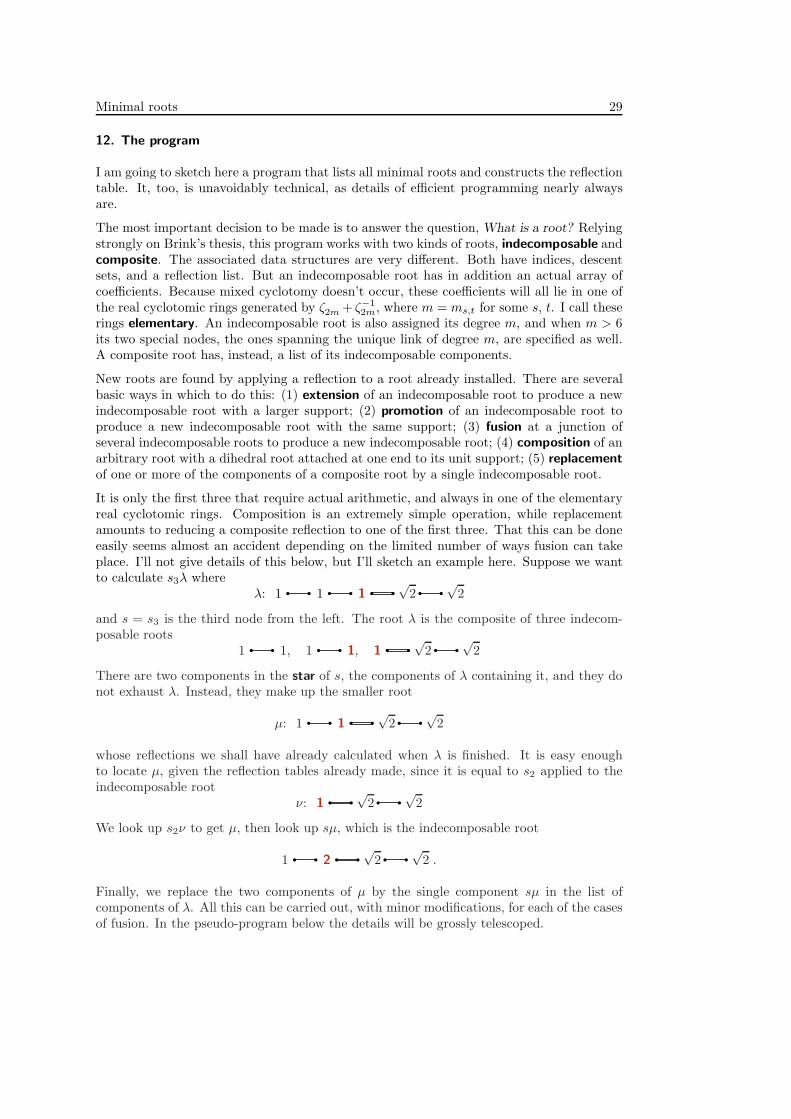
It is only the first three that require actual arithmetic, and always in one of the elementaryreal cyclotomic rings. Composition is an extremely simple operation, while replacementamounts to reducing a composite reflection to one of the first three. That this can be doneeasily seems almost an accident depending on the limited number of ways fusion can takeplace. I’ll not give details of this below, but I’ll sketch an example here. Suppose we wantto calculate s3λ where
λ: 1 1 1√
2√
2
and s = s3 is the third node from the left. The root λ is the composite of three indecom-posable roots
1 1, 1 1, 1√
2√
2
There are two components in the star of s, the components of λ containing it, and they donot exhaust λ. Instead, they make up the smaller root
µ: 1 1√
2√
2
whose reflections we shall have already calculated when λ is finished. It is easy enoughto locate µ, given the reflection tables already made, since it is equal to s2 applied to theindecomposable root
ν: 1√
2√
2
We look up s2ν to get µ, then look up sµ, which is the indecomposable root
1 2√
2√
2 .
Finally, we replace the two components of µ by the single component sµ in the list ofcomponents of λ. All this can be carried out, with minor modifications, for each of the casesof fusion. In the pseudo-program below the details will be grossly telescoped.
Minimal roots 30
The program:
First of all we install the basic roots, those in ∆.
Then we install specially the dihedral roots, those whose support consists of exactly twonodes of the Coxeter graphs. When we are through with these we have finished the basicroots. We put the dihedral roots of depth 2 in the queue, and after we have installed all ofthose we put those of depth 3 in the queue. In this way, we preserve the essential propertyof the queue that roots of depth d are put on before those of depth d + 1.
As for dihedral roots of depth 4 or more, we can finish them as soon as they are installed.Both of their coefficients are 2 or more, which means they cannot be extended, so the onlyreflections higher in the root graph are to dihedral roots with the same support. In otherwords, we never put them in the queue. Incidentally, these occur only for links with m ≥ 6.One consequence is that in calculating reflections of roots taken off the queue, we have onlyto do arithmetic with algebraic integers of the form a + bcm, where m is the degree of theroot, cm = 2 cos(π/m), a and b are integers.
At this point, all roots of depth 1 have been finished, all dihedral roots have been installed,and some have been finished. The queue contains only dihedral roots. While the queue isnot empty, we remove roots from it to be finished.
Let λ be a root removed from the queue. All roots of less depth have been finished already,and in particular all descents sλ ≺ λ have been assigned. We run through all the s in S,and for each one of them where sλ has not been assigned, we have to calculate sλ. Exactlywhat this involves depends on a number of things—the basic idea is to use composition anddecomposition to avoid repeating actual arithmetic.
So now suppose we are looking at s and λ with sλ not known. Let α = αs. There are manycases to deal with.
◦ The node s lies in the support of λ.◦ It belongs to a unique component λi.◦ That component is λ itself, which is therefore indecomposable. We must calculate
the dot product λ •α to see if sλ is minimal or not, and if it is install it.◦ The component λi is not all of λ, which is a composite root. We have calculated sλi
already, and sλ is obtained by replacing λi with sλi.◦ It belongs to several components. It is therefore a junction, and we are looking at
a possible fusion. Let µ be the star of s, the composite of those components whosesupports contain s.◦ The root µ is the same as λ. We have to calculate sλ explicitly. It may be λ, ⊕, or
a new indecomposable root.◦ The root µ makes up only a part of λ. We have calculated sµ, and obtain sλ by
replacing µ with sµ. Exactly what we do to find µ and sµ depends on which case offusion we are dealing with, as I mentioned in the example I looked at earlier. Thiscan be decided by local information around s.
◦ The node s does not lie in the support of λ.◦ It is linked to more than one node in the support, or by a link of infinite degree. Here
sλ = ⊕.◦ It is linked by a single link of finite degree.◦ The link is to a unit node of λ. Then sλ is a new composite.◦ The link is not to a unit node.◦ The root λ is indecomposable. We have to calculate explicitly.
Minimal roots 31
◦ The root λ is composite. If µ is the component it is linked to, we have alreadycalculated sµ. We replace µ by sµ in λ.
In summary, I should say that there are several advantages to following Brink’s idea ofexpressing minimal roots as the amalgamation of indecomposable ones. For one thing,a given indecomposable root may occur in several other roots, so redundancy of storageis eliminated. For another, we only have to do actual arithmetic in promoting nodes ofindecomposable roots, and this amounts to a huge saving in time.
References
1. Brigitte Brink, ‘On root systems and automaticity of Coxeter groups’, Ph. D. thesis,University of Sydney, 1994.
2. Brigitte Brink, ‘The set of dominance-minimal roots’, available as Report 94–43 fromthe School of mathematics and Statistics at the University of Sydney:
http://www.maths.usyd.edu.au:8000/res/Algebra/Bri/dom-min-roots.html
3. Brigitte Brink, ‘The set of dominance-minimal roots’, Journal of Algebra 206 (1998),371–412. This publication, although it has the same title as the previous item, is verydifferent from it. For purposes of computation it is decidedly less interesting, since it doesn’texplicitly introduce the indecomposable minimal roots, and emphasizes hand-lists instead.
4. Brigitte Brink and Robert Howlett, ‘A finiteness property and an automatic structurefor Coxeter groups’, Math. Ann. 296 (1993), 179–190.
5. Bill Casselman, ‘Automata to perform basic calculations in Coxeter groups’, in Repre-sentations of groups, CMS Conference Proceedings 16, A.M.S., 1994.
6. Bill Casselman, ‘Computation in Coxeter groups—I. multiplication’, preprint, 2001.Electronic Journal of Combinatorics 9(1) (2002), #25.
7. Bill Casselman, Java code for finding minimal roots at
http://www.math.ubc.ca/~cass/coxeter.tar.gz
8. Fokko du Cloux, ‘Un algorithme de forme normale pour les groupes de Coxeter’, preprint,Centre de Mathematiques a l’Ecole Polytechnique, 1990.
9. J. Tits, ‘Le probleme des mots dans les groupes de Coxeter’, Symposia Math. 1 (1968),175–185.
10. E. B. Vinberg, ‘Discrete linear groups generated by reflections’, Math. USSR Izvestia5 (1971), 1083–1119.