Frank Bretz, Xiaolei Xun (Novartis) Tutorial at IMPACT … · If multiplicity still persists...
100
Frank Bretz, Xiaolei Xun (Novartis) Tutorial at IMPACT Symposium III November 20, 2014 – Cary NC Introduction to Multiplicity in Clinical Trials
Transcript of Frank Bretz, Xiaolei Xun (Novartis) Tutorial at IMPACT … · If multiplicity still persists...

Frank Bretz, Xiaolei Xun (Novartis)
Tutorial at IMPACT Symposium III
November 20, 2014 – Cary NC
Introduction to Multiplicity in Clinical Trials

Outline
Introduction
Common Multiple Test Procedures
Hierarchical Test Procedure
Closed Test Procedure
Graphical Approach
Summary and Conclusions
2 | IMPACT Symposium III | Frank Bretz | Introduction to Multiple Testing | All Rights Reserved
Introduction
• Type I Error Rate Inflation
• Sources of Multiplicity
• Dealing with Multiplicity
Common Multiple Test Procedures
Hierarchical Test Procedure
Closed Test Procedure
Graphical Approach
Summary and Conclusion
3 | IMPACT Symposium III | Frank Bretz | Introduction to Multiple Testing | All Rights Reserved

Assume that we test a single null hypothesis at significance level 𝛼 = 0.05,
• What is the maximum Type I error rate? 0.05
If we have two null hypotheses and do two independent tests, each at level 𝛼 = 0.05,
• What is the probability of rejecting at least one true null hypothesis?
Pr reject at least one true null = 1 − Pr reject neither true null
= 1 − 0.952
= 0.0975 > 0.05
• The Type I error rate is almost doubled
One possible solution: Test each hypothesis at level 𝛼 2 = 0.025 (Bonferroni test, see later). Then,
Pr reject at least one true null = 0.0494 < 0.05
Type I Error Rate Inflation Simple example with two hypotheses
4 | IMPACT Symposium III | Frank Bretz | Introduction to Multiple Testing | All Rights Reserved

Type I Error Rate Inflation More than two hypotheses
Probability of at least one Type I error
for different number of hypotheses 𝑚 and significance levels 𝛼
• Probability for Type I error
increases with larger
values of 𝑚 and 𝛼
• Example:
For 𝑚 = 10 and 𝛼 = 0.05,
the probability of at least
one Type I error is 40.1%
• For large 𝑚 we almost
surely reject incorrectly at
least one null hypothesis
5 | IMPACT Symposium III | Frank Bretz | Introduction to Multiple Testing | All Rights Reserved

Multiple test problems are very common in clinical trials
Example applications include the comparsion of a new treatment with
• Several other treatments
• A control for more than one endpoint
• A control for more than one population
• A control repeatedly in time
• ... (or any combination thereof)
Multiple test problems in clinical trials are very diverse and many different methods are available
Sources of Multiplicity Overview
6 | IMPACT Symposium III | Frank Bretz | Introduction to Multiple Testing | All Rights Reserved

Reducing the degree of multiplicity by
• Addressing a limited number of questions only
• Minimizing number of variables, using composite endpoints, summary statistics, ...
• Prioritizing questions
If multiplicity still persists
• Multiplicity adjustment should always be considered
• Regulatory guidance (see Appendix) requires a description of the multiplicity adjustment in Phase III study protocols
• If not thought necessary, explain why
Dealing with Multiplicity
7 | IMPACT Symposium III | Frank Bretz | Introduction to Multiple Testing | All Rights Reserved

8 | IMPACT Symposium III | Frank Bretz | Introduction to Multiple Testing | All Rights Reserved
Introduction
Common Multiple Test Procedures
• Basic concepts
• Procedures by
- Bonferroni, Holm
- Simes, Hochberg
- Dunnett, stepwise Dunnett
Hierarchical Test Procedure
Closed Test Procedure
Graphical Approach
Summary and Conclusions

9 | IMPACT Symposium III | Frank Bretz | Introduction to Multiple Testing | All Rights Reserved
Introduction
Common Multiple Test Procedures
• Basic concepts
• Procedures by
- Bonferroni, Holm
- Simes, Hochberg
- Dunnett, stepwise Dunnett
Hierarchical Test Procedure
Closed Test Procedure
Graphical Approach
Summary and Conclusions

Assume a “family” of 𝑚 inferences
Parameters of interest are 𝜃1, … , 𝜃𝑚
Individual null hypotheses
𝐻1: 𝜃1 = 0,… ,𝐻𝑚: 𝜃𝑚 = 0
Example:
• Comparison of 𝑚 treatments with a control therapy
• Then, 𝜃𝑖 = 𝜇𝑖 − 𝜇0 are the 𝑚 treatment effect differences of interest, where
- 𝜇𝑖 denotes the effect for treatment 𝑖 = 1, … ,𝑚
- 𝜇0 denotes the effect for the control therapy
Basic Concepts Notation
10 | IMPACT Symposium III | Frank Bretz | Introduction to Multiple Testing | All Rights Reserved
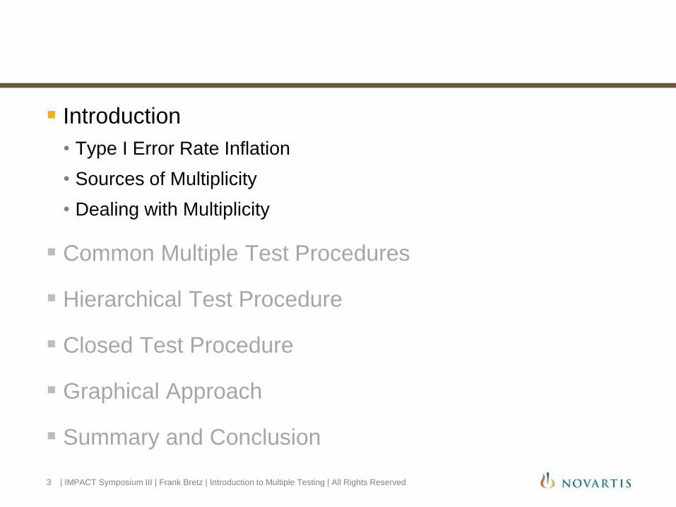
Need to extend the usual Type I error rate concept when testing a family of null hypotheses 𝐻1, … ,𝐻𝑚
A multiple test procedure is said to control the FWER at level 𝛼 (in the strong sense) if
Pr reject at least one true null ≤ 𝛼
under any configuration of true/false null hypotheses
Basic Concepts Family-wise error rate (FWER)
11 | IMPACT Symposium III | Frank Bretz | Introduction to Multiple Testing | All Rights Reserved
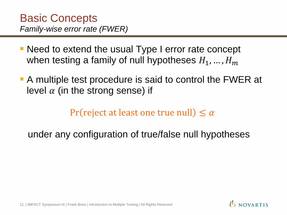
Adjusted p-values extend ordinary (i.e. unadjusted) p-values by adjusting them for a given multiple test procedure
• Adjusted p-values can be compared directly with the significance level 𝛼, while controlling the FWER
Formally, the adjusted p-value is the smallest significance level at which a given hypothesis is significant as part of the multiple test procedure
Example: Bonferroni method
𝑝𝑖 ≤ 𝛼 𝑚 ⇔ 𝑞𝑖 = min 𝑚𝑝𝑖 , 1 ≤ 𝛼
where 𝑝𝑖 is the ordinary and 𝑞𝑖 the adjusted p-value for 𝑖 = 1,… ,𝑚
Basic Concepts Adjusted p-values
12 | IMPACT Symposium III | Frank Bretz | Introduction to Multiple Testing | All Rights Reserved

Single step methods
The rejection or non-rejection of a single hypothesis does not depend
on the decision on any other hypothesis.
Examples: Bonferroni, Simes, Dunnett, …
Stepwise methods
The rejection or non-rejection of a particular hypothesis may depend
on the decision on other hypotheses.
Examples: Holm, Hochberg, stepdown Dunnett, …
Basic Concepts Single step and stepwise test procedures
13 | IMPACT Symposium III | Frank Bretz | Introduction to Multiple Testing | All Rights Reserved

14 | IMPACT Symposium III | Frank Bretz | Introduction to Multiple Testing | All Rights Reserved
Introduction
Common Multiple Test Procedures
• Basic concepts
• Procedures by
- Bonferroni, Holm
- Simes, Hochberg
- Dunnett, stepwise Dunnett
Hierarchical Test Procedure
Closed Test Procedure
Graphical Approach
Summary and Conclusions

Use 𝛼 𝑚 for all inferences; for 𝑖 = 1,… ,𝑚:
Reject 𝐻𝑖 if 𝑝𝑖 ≤ 𝛼 𝑚
Example: With 𝑚 = 3, p-values must be less than 0.05 3 = 0.0167 in order to be “significant”
With adjusted p-values 𝑞𝑖 = min 𝑚𝑝𝑖 , 1 ,
Reject 𝐻𝑖 if 𝑞𝑖 ≤ 𝛼
• Note that 𝑚𝑝𝑖 > 1 is possible and we thus need to truncate the adjusted p-avlues at 1, resulting in the minimum expression
Both rejection rules above lead to the same test decisions
Bonferroni Method Overview
15 | IMPACT Symposium III | Frank Bretz | Introduction to Multiple Testing | All Rights Reserved
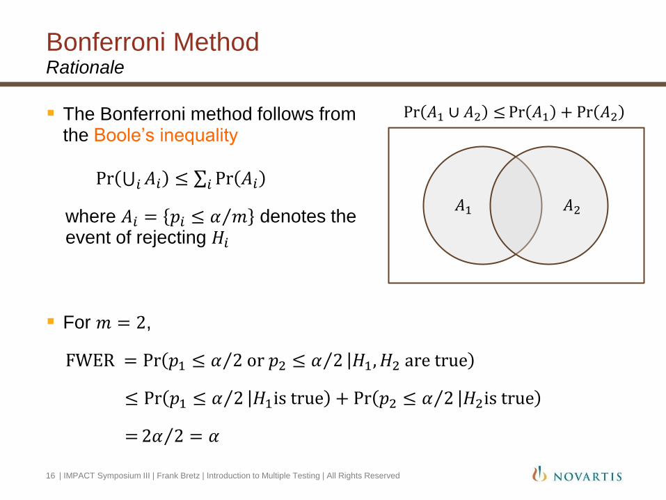
Bonferroni Method Rationale
The Bonferroni method follows from the Boole’s inequality
Pr 𝐴𝑖𝑖 ≤ Pr 𝐴𝑖𝑖
where 𝐴𝑖 = 𝑝𝑖 ≤ 𝛼 𝑚 denotes the event of rejecting 𝐻𝑖
For 𝑚 = 2,
FWER = Pr 𝑝1 ≤ 𝛼 2 or 𝑝2 ≤ 𝛼 2 𝐻1, 𝐻2 are true
≤ Pr 𝑝1 ≤ 𝛼 2 𝐻1is true + Pr 𝑝2 ≤ 𝛼 2 𝐻2is true
=2𝛼 2 = 𝛼
𝐴1 𝐴2
Pr 𝐴1 ∪ 𝐴2 ≤Pr 𝐴1 + Pr 𝐴2
16 | IMPACT Symposium III | Frank Bretz | Introduction to Multiple Testing | All Rights Reserved

The Bonferroni method is a single step procedure
It is rather conservative if:
• The number of hypotheses is large
• The test statistics are strongly positively correlated
The Bonferroni method can be improved:
• Stepwise methods (e.g. Holm procedure; see later)
• Accounting for correlations (e.g. Dunnett test; see later)
While Bonferroni is rarely used in practice, it is the basis for commonly used advanced multiple test procedures
Bonferroni Method Properties
17 | IMPACT Symposium III | Frank Bretz | Introduction to Multiple Testing | All Rights Reserved

Assume p-values 0.0121, 0.0142, 0.0191, 0.1986
Applying Bonferroni, we use 0.05 4 = 0.0125 and reject 𝐻1
However, having rejected 𝐻1 using 0.05 4 , you no longer believe that all four null hypotheses can be true
You now think only 𝐻2, 𝐻3, 𝐻4 can be true
So, test 𝐻2 using 0.05 3 = 0.0167, rather than 0.05 4
Holm Procedure Simplistic explanation
18 | IMPACT Symposium III | Frank Bretz | Introduction to Multiple Testing | All Rights Reserved
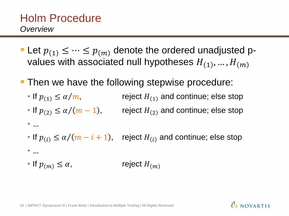
Let 𝑝 1 ≤ ⋯ ≤ 𝑝 𝑚 denote the ordered unadjusted p-
values with associated null hypotheses 𝐻 1 , … ,𝐻 𝑚
Then we have the following stepwise procedure:
• If 𝑝 1 ≤ 𝛼 𝑚 , reject 𝐻 1 and continue; else stop
• If 𝑝 2 ≤ 𝛼 𝑚 − 1 , reject 𝐻 2 and continue; else stop
• …
• If 𝑝 𝑖 ≤ 𝛼 𝑚 − 𝑖 + 1 , reject 𝐻 𝑖 and continue; else stop
• …
• If 𝑝 𝑚 ≤ 𝛼, reject 𝐻 𝑚
Holm Procedure Overview
19 | IMPACT Symposium III | Frank Bretz | Introduction to Multiple Testing | All Rights Reserved

The Holm procedure is a stepwise procedure that is more powerful than the Bonferroni method
• Bonferroni uses the same threshold 𝛼 𝑚 for all hypotheses
• Holm uses the larger thresholds 𝛼 𝑚 − 𝑖 + 1
Sometimes called “stepdown Bonferroni” procedure
The Holm procedure can be improved by accounting for correlations (e.g. stepdown Dunnett test; see later)
Holm Procedure Properties
20 | IMPACT Symposium III | Frank Bretz | Introduction to Multiple Testing | All Rights Reserved

With 𝑝 1 ≤ ⋯ ≤ 𝑝 𝑚 , define adjusted p-values using
• 𝑞 1 = 𝑚𝑝 1
• 𝑞 2 = 𝑚 − 1 𝑝 2 , if 𝑚 − 1 𝑝 2 > 𝑞 1
𝑞 1 , otherwise
• …
• 𝑞 𝑚 = 𝑝 𝑚 , if 𝑝 𝑚 > 𝑞 𝑚−1
𝑞 𝑚−1 , otherwise
Formula for adjusted p-values:
𝑞 1 = min 1,𝑚𝑝 1
𝑞 𝑖 = min 1,max 𝑚 − 𝑖 + 1 𝑝 𝑖 , 𝑞 𝑖−1 , 𝑖 = 2,… ,𝑚
Holm Procedure Adjusted p-Values
21 | IMPACT Symposium III | Frank Bretz | Introduction to Multiple Testing | All Rights Reserved
22 | IMPACT Symposium III | Frank Bretz | Introduction to Multiple Testing | All Rights Reserved
Introduction
Common Multiple Test Procedures
• Basic concepts
• Procedures by
- Bonferroni, Holm
- Simes, Hochberg
- Dunnett, stepwise Dunnett
Hierarchical Test Procedure
Closed Test Procedure
Graphical Approach
Summary and Conclusions

The Simes method tests the global null hypothesis
𝐻 = 𝐻1 ∩ 𝐻2 ∩⋯∩ 𝐻𝑚: 𝜃1 = 𝜃2 = ⋯ = 𝜃𝑚 = 0
It uses all ordered p-values 𝑝 1 , … , 𝑝 𝑚 , not just 𝑝 1
Reject 𝐻 if 𝑝 𝑖 ≤ 𝑖𝛼 𝑚 for at least one 𝑖
Simes’ adjusted p-value uses min𝑖 𝑚𝑝 𝑖 𝑖 , which is less
than or equal to Bonferroni’s 𝑚𝑝 1
Simes cannot be used to test the individual hypotheses 𝐻𝑖
Type I error rate is at most 𝛼 under independence or (certain types of) positive dependence of p-values
Simes Method Overview
23 | IMPACT Symposium III | Frank Bretz | Introduction to Multiple Testing | All Rights Reserved

Bonferroni rejects 𝐻, if 𝑝 1 ≤ 𝛼 2
Simes rejects 𝐻, if 𝑝 1 ≤ 𝛼 2 or 𝑝 2 ≤ 𝛼
Under independence of 𝑝1 and 𝑝2,
• Pr Bonferroni rejects = 1 − 1 − 𝛼 2 2 = 𝛼 − 𝛼 2 2 < 𝛼
• Pr Simes rejects = 1 − 1 − 𝛼 2 2 + 𝛼 2 2 = 𝛼
Simes Method Comparison with Bonferroni method (for 𝑚 = 2)
24 | IMPACT Symposium III | Frank Bretz | Introduction to Multiple Testing | All Rights Reserved
𝑝2
𝑝1
𝛼
0 1
1
𝛼 𝛼 2
𝛼 2
• Simes is more powerful than a
global test based on Bonferroni
• Simes assumes non-negative
correlations between p-values,
Bonferroni does not
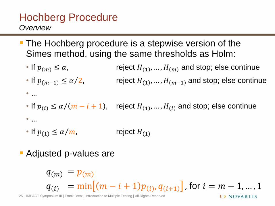
Hochberg Procedure Overview
The Hochberg procedure is a stepwise version of the Simes method, using the same thresholds as Holm:
• If 𝑝 𝑚 ≤ 𝛼, reject 𝐻 1 , … , 𝐻 𝑚 and stop; else continue
• If 𝑝 𝑚−1 ≤ 𝛼 2 , reject 𝐻 1 , … , 𝐻 𝑚−1 and stop; else continue
• …
• If 𝑝 𝑖 ≤ 𝛼 𝑚 − 𝑖 + 1 , reject 𝐻 1 , … , 𝐻 𝑖 and stop; else continue
• …
• If 𝑝 1 ≤ 𝛼 𝑚 , reject 𝐻 1
Adjusted p-values are
𝑞 𝑚 = 𝑝 𝑚
𝑞 𝑖 = min 𝑚 − 𝑖 + 1 𝑝 𝑖 , 𝑞 𝑖+1 , for 𝑖 = 𝑚 − 1,… , 1 25 | IMPACT Symposium III | Frank Bretz | Introduction to Multiple Testing | All Rights Reserved

The Hochberg procedure is sometimes called “stepup Simes” procedure
It is more powerful than the Holm procedure
• Both procedures use the same thresholds, but Hochberg starts with the largest p-value, whereas Holm starts with the smallest
It makes the same assumptions as the Simes test (i.e. independence or positive dependence of p-values)
The Hochberg procedure can be improved
• For example, Hommel procedure based on the closed test procedure (see later)
Hochberg Procedure Properties
26 | IMPACT Symposium III | Frank Bretz | Introduction to Multiple Testing | All Rights Reserved

27 | IMPACT Symposium III | Frank Bretz | Introduction to Multiple Testing | All Rights Reserved
Introduction
Common Multiple Test Procedures
• Basic concepts
• Procedures by
- Bonferroni, Holm
- Simes, Hochberg
- Dunnett, stepwise Dunnett
Hierarchical Test Procedure
Closed Test Procedure
Graphical Approach
Summary and Conclusions

When comparing several treatments with a control, the Dunnett test can be used
The methods from Bonferroni, Holm, Simes, and Hochberg can also be used in these situations, but only the Dunnett test exploits the correlation between the p-values
Dunnett Test Comparing several treatments with a control
28 | IMPACT Symposium III | Frank Bretz | Introduction to Multiple Testing | All Rights Reserved

Consider the unbalanced one-way layout
𝑌𝑖𝑗 = 𝜇𝑖 + 𝜀𝑖𝑗
where
• 𝑌𝑖𝑗 denotes observation 𝑗 = 1,… , 𝑛𝑖 in group 𝑖 = 0,1, … ,𝑚
• 𝜇𝑖 the effect of treatment group 𝑖
• 𝜀𝑖𝑗 are independent and identically normally distributed with mean 0
and variance 𝜎2, i.e. 𝜀𝑖𝑗 ∼ N(0, 𝜎2)
The ANOVA 𝐹-test tests the global null 𝐻: 𝜇0 = ⋯ = 𝜇𝑚
Here, we are interested in comparing 𝑚 treatments with the control treatment 𝑖 = 0, i.e. testing the 𝑚 null hypotheses
𝐻𝑖: 𝜃𝑖 = 𝜇𝑖 − 𝜇0 ≤ 0, 𝑖 = 1,… ,𝑚
Dunnett Test Linear model and hypotheses
29 | IMPACT Symposium III | Frank Bretz | Introduction to Multiple Testing | All Rights Reserved

Consider the 𝑚 pairwise 𝑡-tests
𝑡𝑖 =𝜇 𝑖 − 𝜇 0
𝜎 1𝑛𝑖
+1𝑛0
, 𝑖 = 1,… ,𝑚
where 𝜇 𝑖 and 𝜎 are the ordinary least squares of 𝜇𝑖 and 𝜎, respectively
Note that 𝑡𝑖 ∼ 𝑡𝜈 under 𝐻𝑖, where 𝑡𝜈 denotes the univariate 𝑡-distribution with 𝜈 = 𝑛𝑖𝑖 −𝑚 − 1 degrees of freedom
Furthermore, 𝑡1, … , 𝑡𝑚 follows the 𝑚-variate 𝑡-distribution with 𝜈 degrees of freedom and correlations
𝜌𝑖𝑗 =𝑛𝑖
𝑛𝑖+𝑛0,
𝑛𝑗
𝑛𝑗+𝑛0, 𝑖, 𝑗 = 1,… ,𝑚
Dunnett test Individual test statistics
30 | IMPACT Symposium III | Frank Bretz | Introduction to Multiple Testing | All Rights Reserved

For the 𝑚 individual null hypotheses,
Reject 𝐻𝑖 if 𝑡𝑖 ≥ 𝑐𝑚,1−𝛼
The quantile 𝑐𝑚,1−𝛼 is computed such that
𝑃 𝑡1, … , 𝑡𝑚 ≤ 𝑐𝑚,1−𝛼 , … , 𝑐𝑚,1−𝛼 = 𝑃 max𝑖 𝑡𝑖 ≤ 𝑐𝑚,1−𝛼 = 1 − 𝛼
where 𝑡1, … , 𝑡𝑚 follows the 𝑚-variate 𝑡-distribution with 𝜈 degrees of freedom and correlations 𝜌𝑖𝑗, for 𝑖, 𝑗 = 1,… ,𝑚
In other words, 𝑐𝑚,1−𝛼 is the 1 − 𝛼 quantile of the
distribution of the maximum of 𝑚 𝑡-distributed random variables
Dunnett test Rejection rule
31 | IMPACT Symposium III | Frank Bretz | Introduction to Multiple Testing | All Rights Reserved
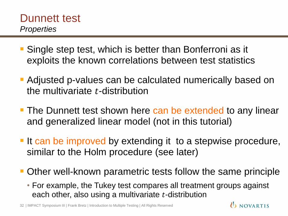
Single step test, which is better than Bonferroni as it exploits the known correlations between test statistics
Adjusted p-values can be calculated numerically based on the multivariate 𝑡-distribution
The Dunnett test shown here can be extended to any linear and generalized linear model (not in this tutorial)
It can be improved by extending it to a stepwise procedure, similar to the Holm procedure (see later)
Other well-known parametric tests follow the same principle
• For example, the Tukey test compares all treatment groups against each other, also using a multivariate 𝑡-distribution
Dunnett test Properties
32 | IMPACT Symposium III | Frank Bretz | Introduction to Multiple Testing | All Rights Reserved

Let 𝑡 1 ≥ ⋯ ≥ 𝑡 𝑚 denote the ordered test statistics with
associated null hypotheses 𝐻 1 , … , 𝐻 𝑚
Then we have the following stepwise procedure:
• If 𝑡 1 ≥ 𝑐𝑚,1−𝛼, reject 𝐻 1 and continue; else stop
• If 𝑡 2 ≥ 𝑐𝑚−1,1−𝛼, reject 𝐻 2 and continue; else stop
• …
• If 𝑡 𝑖 ≥ 𝑐𝑚−𝑖+1,1−𝛼, reject 𝐻 𝑖 and continue; else stop
• …
• If 𝑡 𝑚 ≥ 𝑐1,1−𝛼, reject 𝐻 𝑚
where 𝑐𝑚−𝑖+1,1−𝛼 denotes the 1 − 𝛼 quantile of the distribution of the
maximum of 𝑚 − 𝑖 + 1 𝑡-distributed random variables and is computed from the corresponding multivariate 𝑡-distribution
Stepwise Dunnett test Overview
33 | IMPACT Symposium III | Frank Bretz | Introduction to Multiple Testing | All Rights Reserved

For the stepwise Dunnett test, the quantiles change as hypotheses are rejected
• For example, if 𝐻 1 is rejected, then the quantile 𝑐𝑚−1,1−𝛼 is computed from a
𝑚 − 1 -variate 𝑡-distribution
The stepwise Dunnett test is better than the single step Dunnett test
• It can be shown that 𝑐𝑚,1−𝛼 ≥ 𝑐𝑚−1,1−𝛼 ≥ ⋯ ≥ 𝑐1,1−𝛼, where 𝑐1,1−𝛼 = 𝑡𝜈,1−𝛼 is the
quantile from the univariate 𝑡-distribution with 𝜈 degrees of freedom
• The Dunnett test uses 𝑐𝑚,1−𝛼 for all comparisons
The stepwise Dunnett test is better than the Holm procedure as it exploits the known correlations between test statistics
• The stepwise version shown here is sometimes called “stepdown Dunnett” test
• A “stepup Dunnett” test also exists, similar to Hochberg (not in this tutorial)
Stepwise Dunnett test Properties
34 | IMPACT Symposium III | Frank Bretz | Introduction to Multiple Testing | All Rights Reserved

Correlations
Without With
Single Step Bonferroni Simes Dunnett
Stepwise Holm Hochberg Stepdown Dunnett
Summary
35 | IMPACT Symposium III | Frank Bretz | Introduction to Multiple Testing | All Rights Reserved
Remarks
• Single step methods are less powerful than stepwise methods and not often used in practice
• Accounting for correlations leads to more powerful procedures, but correlations are not always known
• Simes-based methods are more powerful than Bonferroni-based methods, but control the FWER only under certain dependence structures
• In practice, we select the procedure that is not only powerful from a statistical perspective, but also appropriate from clinical perspective

Introduction
Common Multiple Test Procedures
Hierarchical Test Procedure
• Fixed Sequence Procedure
• Fallback Procedure
• Numerical Example
Closed Test Procedure
Graphical Approach
Summary and Conclusions
36 | IMPACT Symposium III | Frank Bretz | Introduction to Multiple Testing | All Rights Reserved
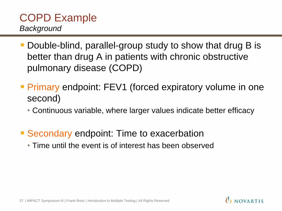
Double-blind, parallel-group study to show that drug B is
better than drug A in patients with chronic obstructive
pulmonary disease (COPD)
Primary endpoint: FEV1 (forced expiratory volume in one
second)
• Continuous variable, where larger values indicate better efficacy
Secondary endpoint: Time to exacerbation
• Time until the event is of interest has been observed
COPD Example Background
37 | IMPACT Symposium III | Frank Bretz | Introduction to Multiple Testing | All Rights Reserved
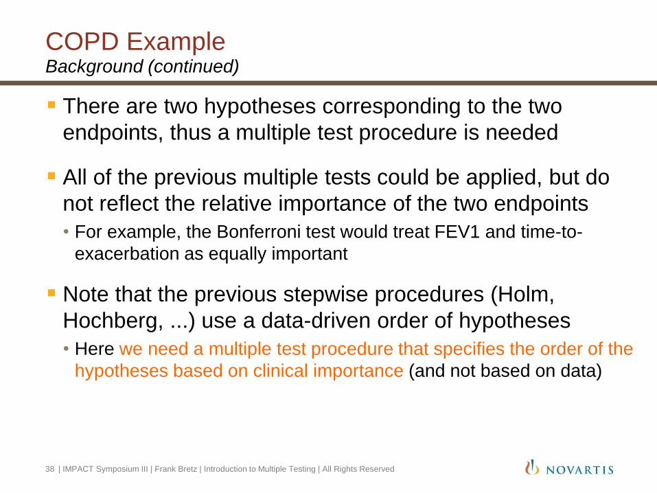
There are two hypotheses corresponding to the two
endpoints, thus a multiple test procedure is needed
All of the previous multiple tests could be applied, but do
not reflect the relative importance of the two endpoints
• For example, the Bonferroni test would treat FEV1 and time-to-
exacerbation as equally important
Note that the previous stepwise procedures (Holm,
Hochberg, ...) use a data-driven order of hypotheses
• Here we need a multiple test procedure that specifies the order of the
hypotheses based on clinical importance (and not based on data)
COPD Example Background (continued)
38 | IMPACT Symposium III | Frank Bretz | Introduction to Multiple Testing | All Rights Reserved

If the hierarchy of hypotheses is specified before data is observed, one can apply a hierarchical test procedure
Two hierarchical test procedures will be introduced
• Fixed sequence procedure
• Fallback procedure
Hierarchical Test Procedures Overview
39 | IMPACT Symposium III | Frank Bretz | Introduction to Multiple Testing | All Rights Reserved
Hierarchical Test Procedures Fixed sequence procedure – General description
40 | IMPACT Symposium III | Frank Bretz | Introduction to Multiple Testing | All Rights Reserved
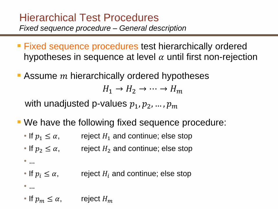
Fixed sequence procedures test hierarchically ordered hypotheses in sequence at level 𝛼 until first non-rejection
Assume 𝑚 hierarchically ordered hypotheses
𝐻1 → 𝐻2 → ⋯ → 𝐻𝑚
with unadjusted p-values 𝑝1, 𝑝2, … , 𝑝𝑚
We have the following fixed sequence procedure:
• If 𝑝1 ≤ 𝛼, reject 𝐻1 and continue; else stop
• If 𝑝2 ≤ 𝛼, reject 𝐻2 and continue; else stop
• …
• If 𝑝𝑖 ≤ 𝛼, reject 𝐻𝑖 and continue; else stop
• …
• If 𝑝𝑚 ≤ 𝛼, reject 𝐻𝑚
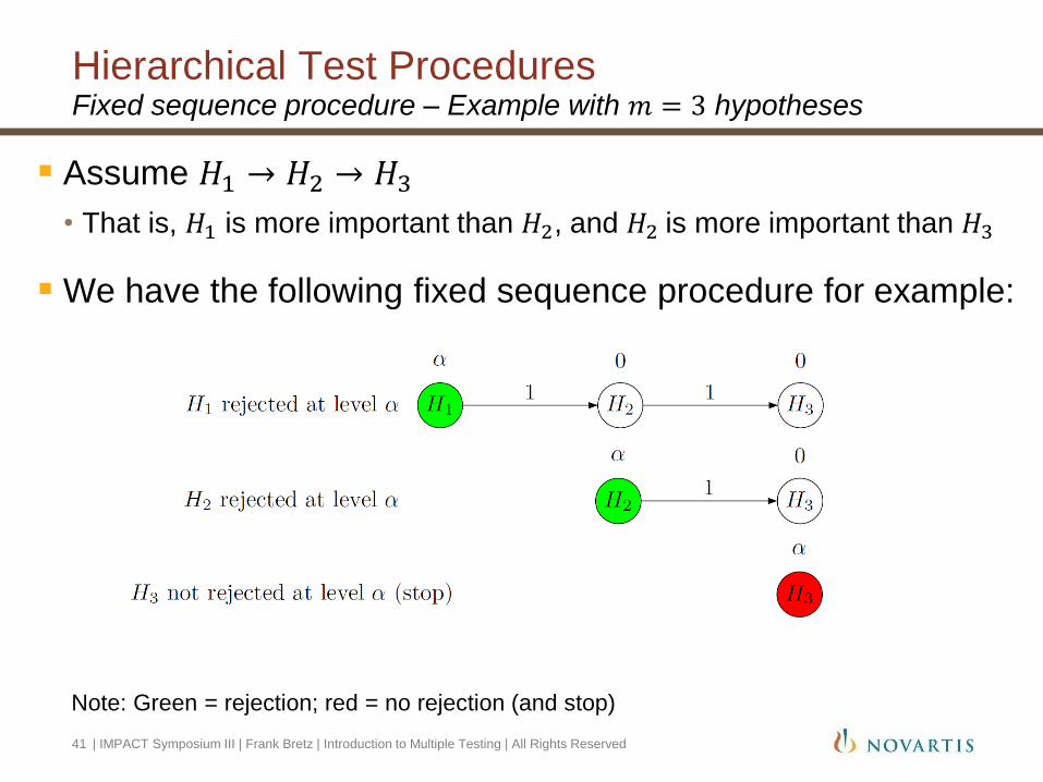
Assume 𝐻1 → 𝐻2 → 𝐻3
• That is, 𝐻1 is more important than 𝐻2, and 𝐻2 is more important than 𝐻3
We have the following fixed sequence procedure for example:
Hierarchical Test Procedures Fixed sequence procedure – Example with 𝑚 = 3 hypotheses
Note: Green = rejection; red = no rejection (and stop)
41 | IMPACT Symposium III | Frank Bretz | Introduction to Multiple Testing | All Rights Reserved

Hierarchical Test Procedures Fixed sequence procedure – Properties
Adjusted p-values are given by
𝑞𝑖 = max 𝑝1, … , 𝑝𝑖 , 𝑖 = 1,… ,𝑚
Advantages
• Simple procedure, each test is performed in sequence at level 𝛼
• It is optimal when hypotheses early in the sequence are associated with large effects and performs poorly otherwise
Disadvantages
• Once a hypothesis is not rejected, no further testing is permitted
Great care is advised when specifying the sequence of hypotheses
42 | IMPACT Symposium III | Frank Bretz | Introduction to Multiple Testing | All Rights Reserved

Hierarchical Test Procedures Fallback procedure – General description
Fallback procedures test hierarchically ordered hypotheses in sequence as the fixed sequence procedure, but splits the level 𝛼 between the hypotheses
Assume 𝑚 hierarchically ordered hypotheses
𝐻1 → 𝐻2 → ⋯ → 𝐻𝑚
with unadjusted p-values 𝑝1, … , 𝑝𝑚 and 𝛼 = 𝛼1 +⋯+ 𝛼𝑚
Then the fallback procedure tests 𝐻𝑖 at level 𝛼𝑖′, where for
𝑖 = 2,… ,𝑚
𝛼𝑖′ =
𝛼𝑖 , if 𝐻𝑖−1 is not rejected
𝛼𝑖 + 𝛼𝑖−1′ , otherwise
and 𝛼1′ = 𝛼1
43 | IMPACT Symposium III | Frank Bretz | Introduction to Multiple Testing | All Rights Reserved

Assume 𝐻1 → 𝐻2 → 𝐻3, and split the significance level as 𝛼1 = 𝛼2 = 𝛼3 = 𝛼/3
Following the fallback procedure, we could have for example:
Hierarchical Test Procedures Fallback procedure – Example with 𝑚 = 3 hypotheses
Note: Green = rejection; red = no rejection (and stop)
44 | IMPACT Symposium III | Frank Bretz | Introduction to Multiple Testing | All Rights Reserved

Hierarchical Test Procedures Fallback procedure – Properties
The fixed sequence procedure is obtained as special case from the fallback procedure by setting 𝛼1 = 𝛼 and 𝛼𝑖 = 0 for 𝑖 > 1
In contrast to the fixed sequence procedure, the fallback procedure tests all hypotheses in the pre-specified sequence even if the initial hypotheses are not rejected
45 | IMPACT Symposium III | Frank Bretz | Introduction to Multiple Testing | All Rights Reserved

Introduction
Common Multiple Test Procedures
Hierarchical Test Procedure
Closed Test Procedure
Graphical Approach
Summary and Conclusions
| IMPACT Symposium III | Frank Bretz | Introduction to Multiple Testing | All Rights Reserved 46
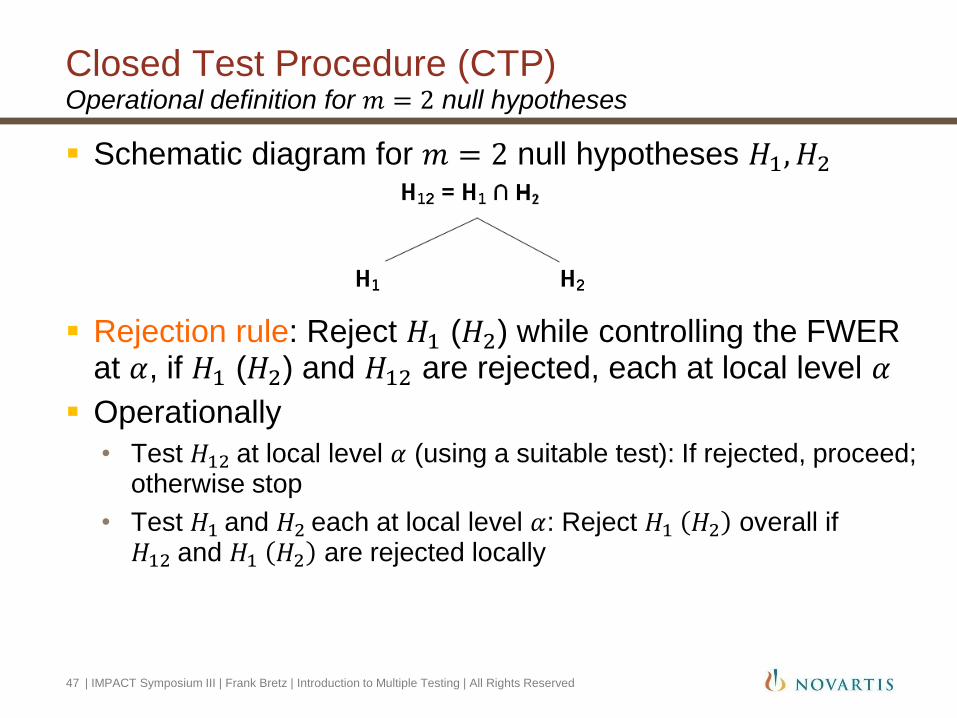
Schematic diagram for 𝑚 = 2 null hypotheses 𝐻1, 𝐻2
Rejection rule: Reject 𝐻1 (𝐻2) while controlling the FWER at 𝛼, if 𝐻1 (𝐻2) and 𝐻12 are rejected, each at local level 𝛼
Operationally
• Test 𝐻12 at local level 𝛼 (using a suitable test): If rejected, proceed; otherwise stop
• Test 𝐻1 and 𝐻2 each at local level 𝛼: Reject 𝐻1 𝐻2 overall if 𝐻12 and 𝐻1 𝐻2 are rejected locally
Closed Test Procedure (CTP) Operational definition for 𝑚 = 2 null hypotheses
47 | IMPACT Symposium III | Frank Bretz | Introduction to Multiple Testing | All Rights Reserved

𝐻1 𝐻2 𝐻12
Closed Test Procedure Venn-type diagram for 𝑚 = 2 null hypotheses
Different parts indicate different null hypotheses as shown above
Question: How do we test them?
• Test 𝐻12 using Bonferroni, Simes, Dunnett, etc. at level 𝛼
• Test 𝐻1, 𝐻2 each using a level 𝛼 test
48 | IMPACT Symposium III | Frank Bretz | Introduction to Multiple Testing | All Rights Reserved
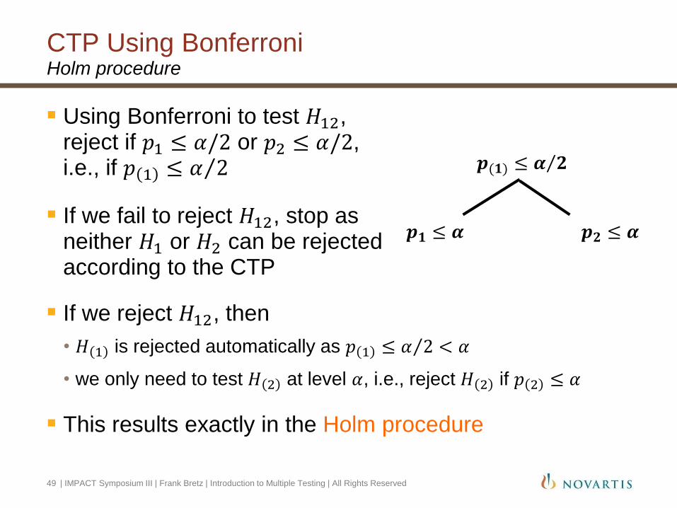
CTP Using Bonferroni Holm procedure
Using Bonferroni to test 𝐻12, reject if 𝑝1 ≤ 𝛼/2 or 𝑝2 ≤ 𝛼/2, i.e., if 𝑝 1 ≤ 𝛼 2
If we fail to reject 𝐻12, stop as neither 𝐻1 or 𝐻2 can be rejected according to the CTP
If we reject 𝐻12, then
• 𝐻 1 is rejected automatically as 𝑝 1 ≤ 𝛼 2 < 𝛼
• we only need to test 𝐻 2 at level 𝛼, i.e., reject 𝐻 2 if 𝑝 2 ≤ 𝛼
This results exactly in the Holm procedure
𝒑(𝟏) ≤ 𝜶 𝟐
𝒑𝟏 ≤ 𝜶 𝒑𝟐 ≤ 𝜶
49 | IMPACT Symposium III | Frank Bretz | Introduction to Multiple Testing | All Rights Reserved

CTP Using Simes Hochberg procedure
Using Simes to test 𝐻12, reject if 𝑝(1) ≤ 𝛼/2 or 𝑝(2) ≤ 𝛼
If we fail to reject 𝐻12, stop
If we reject 𝐻12 because 𝑝(2) ≤ 𝛼, then 𝐻 1 , 𝐻 2 are
rejected automatically as 𝑝 1 ≤ 𝑝 2 ≤ 𝛼, and stop
If we reject 𝐻12 because 𝑝 1 ≤ 𝛼/2 but 𝑝(2) > 𝛼, we then
reject 𝐻(1) but fail to reject 𝐻 2 and stop
This results exactly in the Hochberg procedure for 𝑚 = 2
• For 𝑚 > 2 the Hochberg procedure is less powerful the CTP using Simes tests (Hommel procedure)
𝒑(𝟏) ≤ 𝜶 𝟐 or 𝒑(𝟐) ≤ 𝜶
𝒑𝟏 ≤ 𝜶 𝒑𝟐 ≤ 𝜶
50 | IMPACT Symposium III | Frank Bretz | Introduction to Multiple Testing | All Rights Reserved

CTP Using Dunnett Stepwise Dunnett test
Using Dunnett test to test 𝐻12, reject if 𝑡1 ≤ c2,1−𝛼 or t2 ≤ c2,1−𝛼,
i.e., if 𝑡 1 ≤ c2,1−𝛼
If we fail to reject 𝐻12, stop
If we reject 𝐻12, then
• 𝐻 1 is rejected automatically as 𝑡 1 ≤ c2,1−𝛼 ≤ c1,1−𝛼
• we only need to test 𝐻 2 at level 𝛼, i.e., reject 𝐻 2 if 𝑡 2 ≤ c1,1−𝛼
This results exactly in the stepdown Dunnett procedure
𝒕 𝟏 ≤ 𝒄𝟐,𝟏−𝜶
𝒕𝟏 ≤ 𝒄𝟏,𝟏−𝜶 𝒕𝟐 ≤ 𝒄𝟏,𝟏−𝜶
51 | IMPACT Symposium III | Frank Bretz | Introduction to Multiple Testing | All Rights Reserved
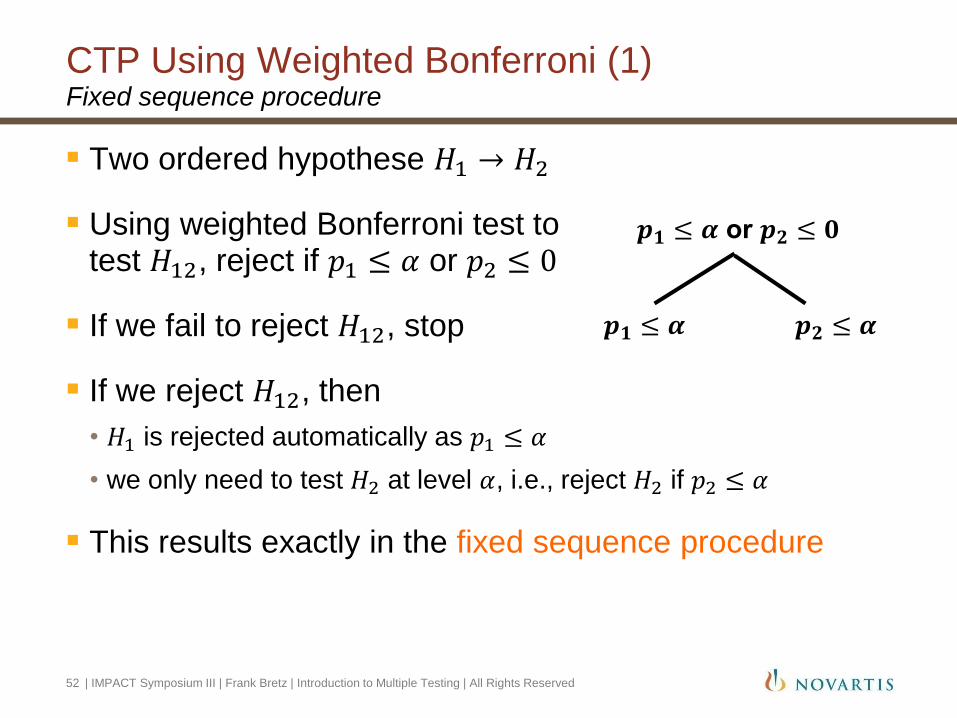
CTP Using Weighted Bonferroni (1) Fixed sequence procedure
Two ordered hypothese 𝐻1 → 𝐻2
Using weighted Bonferroni test to test 𝐻12, reject if 𝑝1 ≤ 𝛼 or 𝑝2 ≤ 0
If we fail to reject 𝐻12, stop
If we reject 𝐻12, then
• 𝐻1 is rejected automatically as 𝑝1 ≤ 𝛼
• we only need to test 𝐻2 at level 𝛼, i.e., reject 𝐻2 if 𝑝2 ≤ 𝛼
This results exactly in the fixed sequence procedure
𝒑𝟏 ≤ 𝜶 or 𝒑𝟐 ≤ 𝟎
𝒑𝟏 ≤ 𝜶 𝒑𝟐 ≤ 𝜶
52 | IMPACT Symposium III | Frank Bretz | Introduction to Multiple Testing | All Rights Reserved

CTP Using Weighted Bonferroni (2) Fallback procedure
Two ordered hypothese 𝐻1 → 𝐻2
Using weighted Bonferroni test to test 𝐻12, reject if 𝑝1 ≤ 𝛼1 or 𝑝2 ≤ 𝛼2
• Weights 𝛼1 and 𝛼2 are such that 𝛼1 + 𝛼2 = 𝛼
If we fail to reject 𝐻12, stop
If we reject 𝐻12, then we test 𝐻2 at level 𝛼, i.e., reject 𝐻2 if 𝑝2 ≤ 𝛼
• 𝐻1 is tested at 𝛼1 level instead of 𝛼
This results exactly in the fallback procedure
𝒑𝟏 ≤ 𝜶𝟏 or 𝒑𝟐 ≤ 𝜶𝟐
𝒑𝟏 ≤ 𝜶𝟏 𝒑𝟐 ≤ 𝜶
53 | IMPACT Symposium III | Frank Bretz | Introduction to Multiple Testing | All Rights Reserved
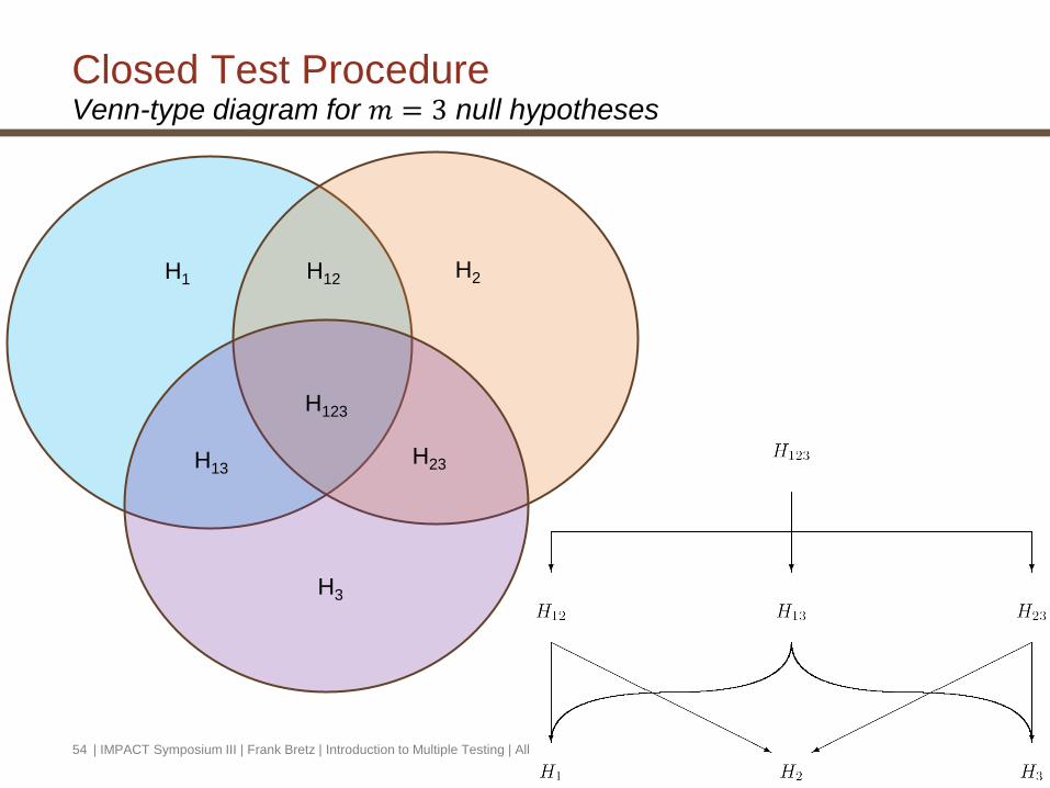
Closed Test Procedure Venn-type diagram for 𝑚 = 3 null hypotheses
54 | IMPACT Symposium III | Frank Bretz | Introduction to Multiple Testing | All Rights Reserved
H1 H2 H12
H123
H13 H23
H3
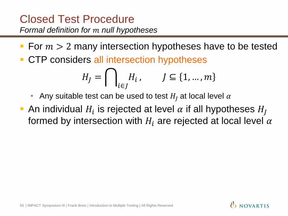
For 𝑚 > 2 many intersection hypotheses have to be tested
CTP considers all intersection hypotheses
𝐻𝐽 = 𝐻𝑖𝑖∈𝐽
, 𝐽 ⊆ 1,… ,𝑚
• Any suitable test can be used to test 𝐻𝐽 at local level 𝛼
An individual 𝐻𝑖 is rejected at level 𝛼 if all hypotheses 𝐻𝐽
formed by intersection with 𝐻𝑖 are rejected at local level 𝛼
Closed Test Procedure Formal definition for 𝑚 null hypotheses
55 | IMPACT Symposium III | Frank Bretz | Introduction to Multiple Testing | All Rights Reserved

| IMPACT Symposium III | Frank Bretz | Introduction to Multiple Testing | All Rights Reserved 56
Summary
CTP is a general principle to construct powerful multiple test procedures
In a CTP, one rejects an individual null hypothesis 𝐻𝑖 at overall level 𝛼 by rejecting all intersection null hypotheses 𝐻𝐽 ⊆ 𝐻𝑖, including 𝐽 = 𝑖
Many common multiple test procedures are CTP, including
• Holm, Hochberg, step-down Dunnett, ...
CTPs satisfy certain optimality criteria and there is no reason why not to use a CTP
The number of intersection hypotheses is 2𝑚 − 1
• For large 𝑚, this number increases rapidly and CTPs are in general difficult to apply

| IMPACT Symposium III | Frank Bretz | Introduction to Multiple Testing | All Rights Reserved 57
Introduction
Common Multiple Test Procedures
Hierarchical Test Procedure
Closed Test Procedure
Graphical Approach
• Conventions
• Common multiple test procedures
• Formal description
• COPD example extended
Summary and Conclusions

| IMPACT Symposium III | Frank Bretz | Introduction to Multiple Testing | All Rights Reserved 58
Introduction
Common Multiple Test Procedures
Hierarchical Test Procedure
Closed Test Procedure
Graphical Approach
• Conventions
• Common multiple test procedures
• Formal description
• COPD example extended
Summary and Conclusions

Objective: Show that a new drug is better than a control drug in patients with COPD for two endpoints
• Primary endpoint: FEV1 (forced expiratory volume in one second)
- Continuous variable, where larger values indicate better efficacy
• Secondary endpoint: Time to exacerbation
- Time until the event of interest has been observed
New drug is available at two doses 𝐷1, 𝐷2 that are compared with the control 𝐶
COPD Example extended Multiple endpoints and multiple doses
59 | IMPACT Symposium III | Frank Bretz | Introduction to Multiple Testing | All Rights Reserved
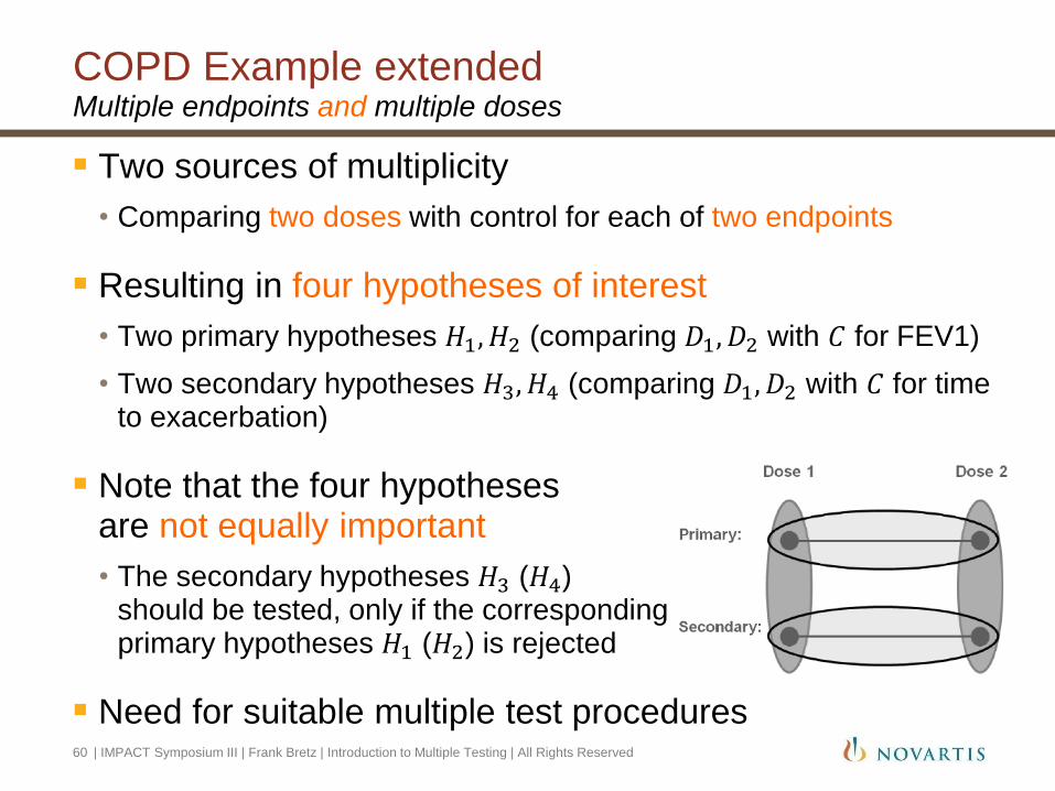
Two sources of multiplicity
• Comparing two doses with control for each of two endpoints
Resulting in four hypotheses of interest
• Two primary hypotheses 𝐻1, 𝐻2 (comparing 𝐷1, 𝐷2 with 𝐶 for FEV1)
• Two secondary hypotheses 𝐻3, 𝐻4 (comparing 𝐷1, 𝐷2 with 𝐶 for time to exacerbation)
Note that the four hypotheses are not equally important
• The secondary hypotheses 𝐻3 (𝐻4) should be tested, only if the corresponding primary hypotheses 𝐻1 (𝐻2) is rejected
Need for suitable multiple test procedures
COPD Example extended Multiple endpoints and multiple doses
60 | IMPACT Symposium III | Frank Bretz | Introduction to Multiple Testing | All Rights Reserved
As before,
• Null hypotheses 𝐻1, … , 𝐻𝑚
• Initial allocation of the significance level 𝛼1 +⋯+ 𝛼𝑚 = 𝛼
• Unadjusted p-values 𝑝1, … , 𝑝𝑚
𝛼–propagation
If a hypothesis 𝐻𝑖 can be rejected at level 𝛼𝑖 (i.e. 𝑝𝑖 ≤ 𝛼𝑖), propagate its level 𝛼𝑖 to the remaining, not yet rejected hypotheses (according to a prefixed rule) and continue testing with the updated 𝛼 levels
Graphical Approach Heuristics
61 | IMPACT Symposium III | Frank Bretz | Introduction to Multiple Testing | All Rights Reserved
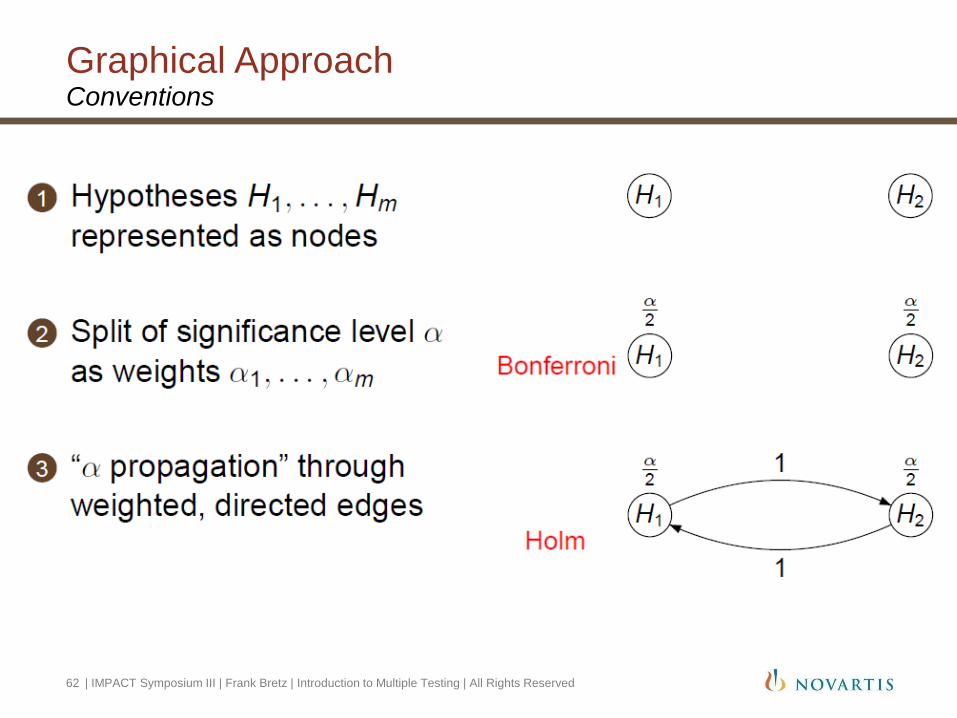
Graphical Approach Conventions
62 | IMPACT Symposium III | Frank Bretz | Introduction to Multiple Testing | All Rights Reserved

| IMPACT Symposium III | Frank Bretz | Introduction to Multiple Testing | All Rights Reserved 63
Introduction
Common Multiple Test Procedures
Hierarchical Test Procedure
Closed Test Procedure
Graphical Approach
• Conventions
• Common multiple test procedures
• Formal description
• COPD example extended
Summary and Conclusions

Bonferroni: no 𝛼–propagation, i.e. no edges between nodes
Holm: includes 𝛼–propagation and is thus more powerful
Graphical Approach Bonferroni test and Holm procedure: m=2
64 | IMPACT Symposium III | Frank Bretz | Introduction to Multiple Testing | All Rights Reserved

Graphical Approach Holm procedure: Example with 𝛼 = 0.025
Test 𝐻1 at level 𝛼/2 Test 𝐻2 at level 𝛼/2
65 | IMPACT Symposium III | Frank Bretz | Introduction to Multiple Testing | All Rights Reserved

Graphical Approach Holm procedure: Example with 𝛼 = 0.025
𝑝2 < 𝛼 2 ⟹ reject 𝐻2
66 | IMPACT Symposium III | Frank Bretz | Introduction to Multiple Testing | All Rights Reserved

Graphical Approach Holm procedure: Example with 𝛼 = 0.025
Propagate 𝛼/2
67 | IMPACT Symposium III | Frank Bretz | Introduction to Multiple Testing | All Rights Reserved

Graphical Approach Holm procedure: Example with 𝛼 = 0.025
Remove node for 𝐻2
68 | IMPACT Symposium III | Frank Bretz | Introduction to Multiple Testing | All Rights Reserved

Graphical Approach Holm procedure: Example with 𝛼 = 0.025
Test 𝐻1 at level 𝛼
𝑝1 > 𝛼 ⟹ retain 𝐻1 and stop
69 | IMPACT Symposium III | Frank Bretz | Introduction to Multiple Testing | All Rights Reserved

Graphical Approach Weighted Holm procedure
Use 𝛼1, 𝛼2 with 𝛼1 + 𝛼2 = 𝛼 instead of 𝛼1 = 𝛼2 = 𝛼/2
70 | IMPACT Symposium III | Frank Bretz | Introduction to Multiple Testing | All Rights Reserved

Graphical Approach Fixed sequence procedure: Example with 𝑚 = 3 hypotheses
Assume 𝐻1 → 𝐻2 → 𝐻3
• That is, 𝐻1 is more important than 𝐻2, and 𝐻2 is more important than 𝐻3
Then we could have, for example, the following fixed sequence procedure:
Note: Green = rejection; red = no rejection (and stop)
71 | IMPACT Symposium III | Frank Bretz | Introduction to Multiple Testing | All Rights Reserved

Graphical Approach Fallback procedure: Example with 𝑚 = 3 hypotheses
Assume 𝐻1 → 𝐻2 → 𝐻3, and split the significance level as 𝛼1 = 𝛼2 = 𝛼3 = 𝛼/3
Then we could have, for example, the following fallback procedure:
72 | IMPACT Symposium III | Frank Bretz | Introduction to Multiple Testing | All Rights Reserved

| IMPACT Symposium III | Frank Bretz | Introduction to Multiple Testing | All Rights Reserved 73
Introduction
Common Multiple Test Procedures
Hierarchical Test Procedure
Closed Test Procedure
Graphical Approach
• Conventions
• Common multiple test procedures
• Formal description
• COPD example extended
Summary and Conclusions
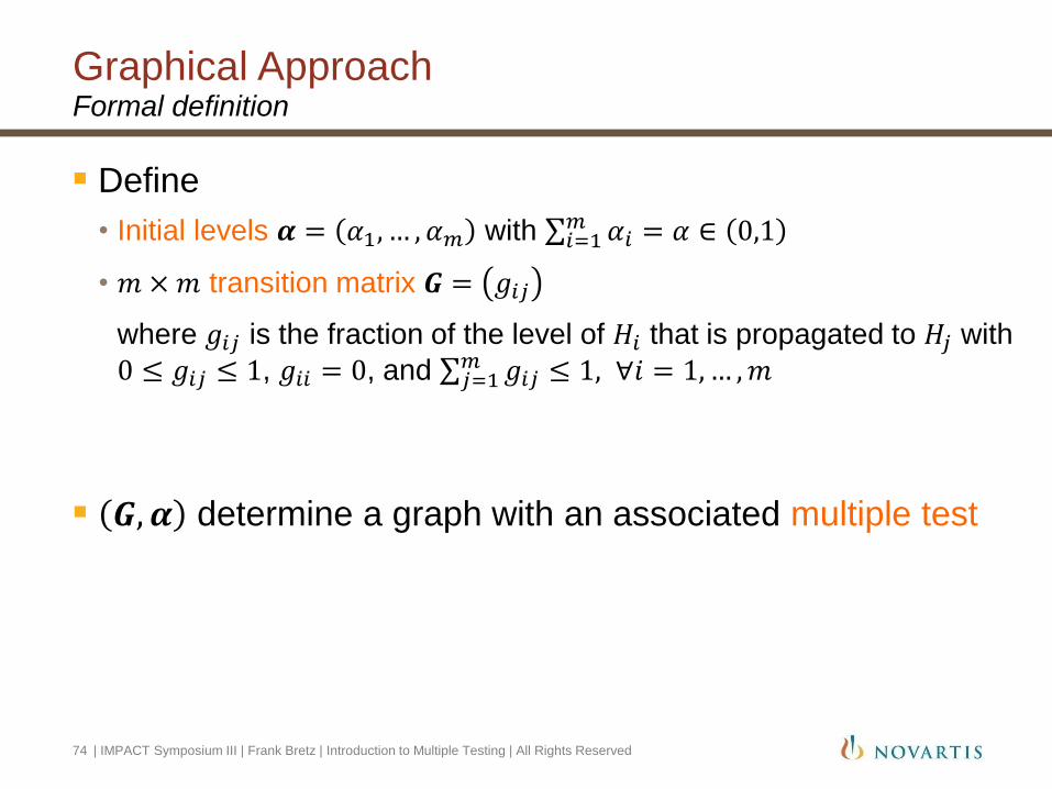
Graphical Approach Formal definition
Define
• Initial levels 𝜶 = 𝛼1, … , 𝛼𝑚 with 𝛼𝑖𝑚𝑖=1 = 𝛼 ∈ 0,1
• 𝑚 ×𝑚 transition matrix 𝑮 = 𝑔𝑖𝑗
where 𝑔𝑖𝑗 is the fraction of the level of 𝐻𝑖 that is propagated to 𝐻𝑗 with
0 ≤ 𝑔𝑖𝑗 ≤ 1, 𝑔𝑖𝑖 = 0, and 𝑔𝑖𝑗𝑚𝑗=1 ≤ 1, ∀𝑖 = 1,… ,𝑚
𝑮,𝜶 determine a graph with an associated multiple test
74 | IMPACT Symposium III | Frank Bretz | Introduction to Multiple Testing | All Rights Reserved

Graphical Approach Update algorithm
Set 𝐽 = 1,… ,𝑚
❶ Select a 𝑗 such that 𝑝𝑗 ≤ 𝛼𝑗
If no such 𝑗 exists, stop; otherwise reject 𝐻𝑗
❷ Update the graph:
𝐽 → 𝐽 ∖ 𝑗
𝛼ℓ → 𝛼ℓ + 𝛼𝑗𝑔𝑗ℓ, ℓ ∈ 𝐽
0, otherwise
𝑔ℓ𝑚 → 𝑔ℓ𝑚+𝑔ℓ𝑗𝑔𝑗𝑚
1−𝑔ℓ𝑗𝑔𝑗ℓ, ℓ,𝑚 ∈ 𝐽, ℓ ≠ 𝑚, 𝑔ℓ𝑗𝑔𝑗ℓ < 1
0, otherwise
❸ Go to Step 1
75 | IMPACT Symposium III | Frank Bretz | Introduction to Multiple Testing | All Rights Reserved

Graphical Approach Main result
The initial levels 𝜶, the transition matrix 𝑮, and the algorithm define a unique sequentially rejective test procedure that controls the FWER at level 𝛼
Remarks:
• Any multiple test procedure derived and visualized by a graph 𝑮,𝜶 is based on the closed test principle
• The graph 𝑮,𝜶 and the algorithm define weighted Bonferroni tests for each intersection hypothesis in a CTP
• The algorithm defines a shortcut for the resulting CTP, which does not depend on the rejection sequence
76 | IMPACT Symposium III | Frank Bretz | Introduction to Multiple Testing | All Rights Reserved
| IMPACT Symposium III | Frank Bretz | Introduction to Multiple Testing | All Rights Reserved 77
Introduction
Common Multiple Test Procedures
Hierarchical Test Procedure
Closed Test Procedure
Graphical Approach
• Conventions
• Common multiple test procedures
• Formal description
• COPD example extended
Summary and Conclusions
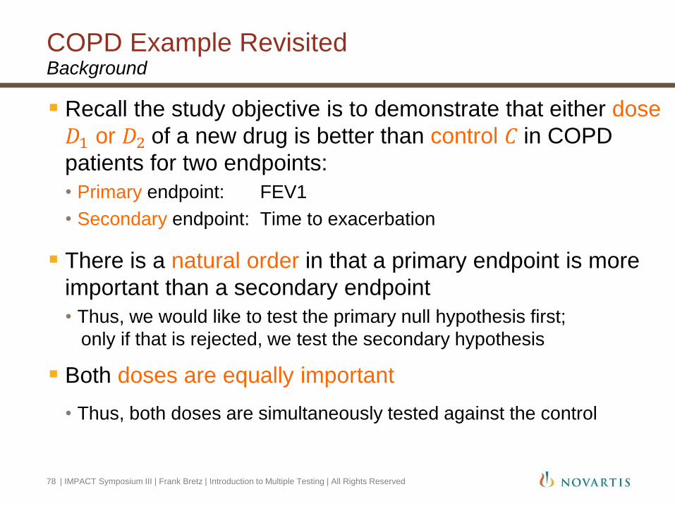
Recall the study objective is to demonstrate that either dose
𝐷1 or 𝐷2 of a new drug is better than control 𝐶 in COPD
patients for two endpoints:
• Primary endpoint: FEV1
• Secondary endpoint: Time to exacerbation
There is a natural order in that a primary endpoint is more
important than a secondary endpoint
• Thus, we would like to test the primary null hypothesis first;
only if that is rejected, we test the secondary hypothesis
Both doses are equally important
• Thus, both doses are simultaneously tested against the control
COPD Example Revisited Background
78 | IMPACT Symposium III | Frank Bretz | Introduction to Multiple Testing | All Rights Reserved

We have four hypotheses corresponding to the two doses
and the two endpoints; a multiple test procedure is needed
Standard multiple test procedures could be applied, but do
not reflect the relative importance of the two endpoints
• For example, the Bonferroni test would treat FEV1 and time-to-
exacerbation as equally important and doesn’t reflect the relative
order desired
We need a multiple test procedure that reflects the relative
importance and order of the hypotheses based on clinical
importance
COPD Example Revisited Background (continued)
79 | IMPACT Symposium III | Frank Bretz | Introduction to Multiple Testing | All Rights Reserved

COPD Example Revisited Building a multiple test procedure: Hypotheses
80 | IMPACT Symposium III | Frank Bretz | Introduction to Multiple Testing | All Rights Reserved

COPD Example Revisited Building a multiple test procedure: Initial levels 𝜶
81 | IMPACT Symposium III | Frank Bretz | Introduction to Multiple Testing | All Rights Reserved

COPD Example Revisited Building a multiple test procedure: 𝛼–propagation
82 | IMPACT Symposium III | Frank Bretz | Introduction to Multiple Testing | All Rights Reserved
𝜶 = 𝛼2
𝛼2 0 0
𝑮 =
0 00 0
1 00 1
0 11 0
0 00 0

COPD Example Revisited Building a multiple test procedure: Alternative 𝛼–propagation
83 | IMPACT Symposium III | Frank Bretz | Introduction to Multiple Testing | All Rights Reserved
𝜶 = 𝛼2
𝛼2 0 0
𝑮 =
0 12
12 0
12
0
0 12
0 11 0
0 00 0

COPD Example Revisited Building a multiple test procedure: General solution
Resulting graph depends on only three
parameters 𝛼1, 𝛾1, and 𝛾2 that can be
finetuned based on:
• further clinical considerations, or
• assumptions about effect sizes, correlations, ...
84 | IMPACT Symposium III | Frank Bretz | Introduction to Multiple Testing | All Rights Reserved
𝜶 = 𝛼1 𝛼2 0 0
𝑮 =
0 𝛾1𝛾2 0
1 − 𝛾1 00 1 − 𝛾2
0 11 0
0 00 0

COPD Example Revisited Numerical example with 𝛼 = 0.025
85 | IMPACT Symposium III | Frank Bretz | Introduction to Multiple Testing | All Rights Reserved

COPD Example Revisited Numerical example with 𝛼 = 0.025
86 | IMPACT Symposium III | Frank Bretz | Introduction to Multiple Testing | All Rights Reserved
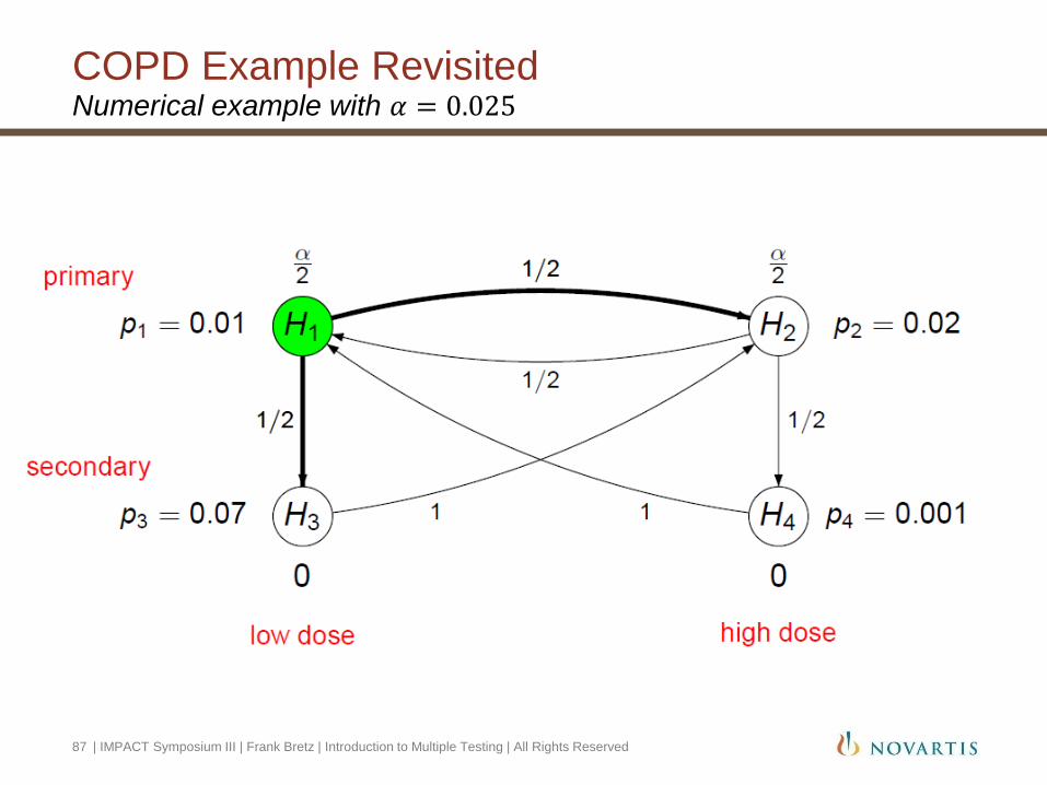
COPD Example Revisited Numerical example with 𝛼 = 0.025
87 | IMPACT Symposium III | Frank Bretz | Introduction to Multiple Testing | All Rights Reserved

COPD Example Revisited Numerical example with 𝛼 = 0.025
88 | IMPACT Symposium III | Frank Bretz | Introduction to Multiple Testing | All Rights Reserved
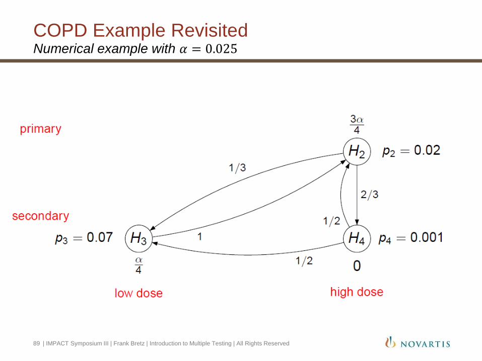
COPD Example Revisited Numerical example with 𝛼 = 0.025
89 | IMPACT Symposium III | Frank Bretz | Introduction to Multiple Testing | All Rights Reserved

COPD Example Revisited Numerical example with 𝛼 = 0.025
90 | IMPACT Symposium III | Frank Bretz | Introduction to Multiple Testing | All Rights Reserved

COPD Example Revisited SAS: Main function
91 | IMPACT Symposium III | Frank Bretz | Introduction to Multiple Testing | All Rights Reserved
/* h: indicator whether a hypothesis is rejected (= 1) or not (= 0) (1 x n vector) a: initial significance level allocation (1 x n vector) w: weights for the edges (n x n matrix) p: observed p-values (1 x n vector) */ START mcp(h, a, w, p); n = NCOL(h); mata = a; crit = 0; DO UNTIL(crit = 1); test = (p < a); IF (ANY(test)) THEN DO; rej = MIN(LOC(test#(1:n))); h[rej] = 1; w1 = J(n, n, 0); DO i = 1 TO n; a[i] = a[i] + a[rej]*w[rej,i]; IF (w[i,rej]*w[rej,i]<1) THEN DO j = 1 TO n; w1[i,j] = (w[i,j] + w[i,rej]*w[rej,j])/(1 - w[i,rej]*w[rej,i]); END; w1[i,i] = 0; END; w = w1; w[rej,] = 0; w[,rej] = 0; a[rej] = 0; mata = mata // a; END; ELSE crit = 1; END; PRINT h; PRINT (ROUND(mata, 0.0001)); PRINT (ROUND(w,0.01)); FINISH;

COPD Example Revisited SAS: Example call
START mcp(h, a, w, p); ... FINISH; /*** Numerical example ***/ h = {0 0 0 0 }; a = {0.0125 0.0125 0 0 }; w = {0 0.5 0.5 0 , 0.5 0 0 0.5 , 0 1 0 0 , 1 0 0 0 }; p = {0.01 0.02 0.07 0.001}; RUN mcp(h, a, w, p); QUIT;
92 | IMPACT Symposium III | Frank Bretz | Introduction to Multiple Testing | All Rights Reserved

Open source package at http://cran.r-project.org/web/packages/gMCP/
Provide graphical user interface (GUI) within R through JAVA
COPD Example Revisited R: gMCP package
93 | IMPACT Symposium III | Frank Bretz | Introduction to Multiple Testing | All Rights Reserved
Proposed graphical approach offers the possibility to
• Tailor advanced multiple test procedures to structured families of hypotheses,
• Visualize complex decision strategies in an efficient and easily communicable way, and
• Ensure strong FWER control
Approach covers many common multiple test procedures as special cases
• Holm, fixed sequence, fallback, gatekeeping, ...
Summary
94 | IMPACT Symposium III | Frank Bretz | Introduction to Multiple Testing | All Rights Reserved

Introduction
Common Multiple Test Procedures
Hierarchical Test Procedure
Closed Test Procedure
Graphical Approach
Summary and Conclusions
| IMPACT Symposium III | Frank Bretz | Introduction to Multiple Testing | All Rights Reserved 95

Multiplicity raises challenging problems which affect almost every decision throughout drug development
Closed test procedure is a general principle to construct powerful multiple test procedures; many common procedures are CTPs
For structured hypotheses, one can apply the graphical approach, which is based on CTPs
• Reflect the difference in importance as well as the relationship between the various study objectives
• Are often applied to clinical trials with structured families of hypotheses and several levels of multiplicity
| IMPACT Symposium III | Frank Bretz | Introduction to Multiple Testing | All Rights Reserved 96
Summary

It is critical to choose the suitable method for a particular problem
There are different types of multiplicity problems that need other methods than those described here, such as:
• Safety data analyses
• Large-scale testing in genetics, proteomics etc.
• Post-hoc analyses / data snooping
| IMPACT Symposium III | Frank Bretz | Introduction to Multiple Testing | All Rights Reserved 97
Summary

Q & A
| IMPACT Symposium III | Frank Bretz | Introduction to Multiple Testing | All Rights Reserved 98

Appendix Main References
99 | IMPACT Symposium III | Frank Bretz | Introduction to Multiple Testing | All Rights Reserved
Alosh, M., Bretz, F., and Huque, M. (2014) Advanced multiplicity adjustment methods in clinical trials. Statistics in Medicine 33(4), 693-713.
Bretz, F., Maurer, W. and Maca J. (2014) Graphical Approaches to Multiple Testing. To appear as Chapter 14 in: Clinical Trial Biostatistics and Biopharmaceutical Applications (ed: Walter Young and Ding-Geng (Din) Chen), Taylor and Francis, Boca Raton
Bretz, F., Hothorn, T., and Westfall, P. (2010). Multiple Comparisons with R. Chapman and Hall, Boca Raton.
Dmitrienko, A., Tamhane, A. C. and Bretz, F. (Eds.) (2009). Multiple Testing Problems in Pharmaceutical Statistics. Chapman & Hall/CRC Biostatistics Series, Boca Raton.
Westfall, P., Tobias, R. and Wolfinger, R. (2011). Multiple Comparisons and Multiple Tests Using SAS. SAS Press, Cary, NC.

Appendix Regulatory Guidelines
ICH E9 (1998) on “Statistical principles for clinical trials”
CPMP (2002) Points to consider on “Multiplicity issues in clinical trials”
FDA draft guidance for industry on “Multiple endpoint analyses” expected for 2014
100 | IMPACT Symposium III | Frank Bretz | Introduction to Multiple Testing | All Rights Reserved