FPGA ASI INTELLIGENT ONTROL IMPLEMENTATION FOR … · FPGA basic intelligent ... through the...

FPGA BASIC INTELLIGENT CONTROL IMPLEMENTATION FOR

HRRTCS

Evelyn González-Hernández

Dr. Gengis K. Toledo-Ramírez

July 29, 2016

FPGA basic intelligent control implementation for HRRTCS

Page 1 of 29

CONTENTS OBJETIVE.............................................................................................................................................. 1

BASIC CONCEPTS AND THEORY ........................................................................................................... 1

INTELLIGENT SYSTEMS .................................................................................................................... 1

ARTIFICIAL NEURAL NETWORK ....................................................................................................... 2

Background.................................................................................................................................. 3

History ......................................................................................................................................... 4

Employing artificial neural networks .......................................................................................... 6

Applications ................................................................................................................................. 6

PERCEPTRON ................................................................................................................................... 8

Definitions ................................................................................................................................... 9

Steps .......................................................................................................................................... 10

Convergence .............................................................................................................................. 10

FPGA .............................................................................................................................................. 11

ARTY .......................................................................................................................................... 12

VHDL .......................................................................................................................................... 14

PROJECT DEVELOPMENT ................................................................................................................... 15

IMPLEMENTATION OF PERCEPTRONS ........................................................................................... 18

RESULTS ............................................................................................................................................. 26

CONCLUSION ..................................................................................................................................... 27

ACKNOWLEDGMENTS ....................................................................................................................... 28

REFERENCES ...................................................................................................................................... 28

OBJETIVE This project is aimed to make a basic perceptron design in the FPGA DILIGENT ARTIX 7

through the software tool Vivado Design Suite in VHDL language, with the aim of laying the

foundation, tools and techniques for development with FPGAs in intelligent systems.

BASIC CONCEPTS AND THEORY

INTELLIGENT SYSTEMS An intelligent system is a machine with an embedded, Internet-connected computer that has

the capacity to gather and analyze data and communicate with other systems.

Requirements for an intelligent system include security, connectivity, the ability to adapt

according to current data and the capacity for remote monitoring and management.


Page 2 of 29

Essentially, an intelligent system is anything that contains a functional, although not usually

general-purpose, computer with Internet connectivity. An embedded system may be

powerful and capable of complex processing and data analysis, but it is usually specialized

for tasks relevant to the host machine.

Intelligent systems exist all around us in point-of-sale terminals, digital televisions, traffic

lights, smart meters, automobiles, digital signage and airplane controls, among a great

number of other possibilities. As this ongoing trend continues, many foresee a scenario

known as the Internet of Things, in which objects, animals and people can all be provided

with unique identifiers and the ability to automatically transfer data over a network without

requiring human-to-human or human-to-computer interaction.

ARTIFICIAL NEURAL NETWORK In machine learning and cognitive science, artificial neural networks (ANNs) are a family of

models inspired by biological neural networks (the central nervous systems of animals, in

particular the brain) which are used to estimate or approximate functions that can depend

on a large number of inputs and are generally unknown. Artificial neural networks are

typically specified using three things:

Architecture specifies what variables are involved in the network and their topological

relationships—for example the variables involved in a neural network might be the weights

of the connections between the neurons, along with activities of the neurons

Activity Rule Most neural network models have short time-scale dynamics: local rules define

how the activities of the neurons change in response to each other. Typically, the activity

rule depends on the weights (the parameters) in the network.

Learning Rule The learning rule specifies the way in which the neural network's weights

change with time. This learning is usually viewed as taking place on a longer time scale than

the time scale of the dynamics under the activity rule. Usually the learning rule will depend

on the activities of the neurons. It may also depend on the values of the target values

supplied by a teacher and on the current value of the weights.

For example, a neural network for handwriting recognition is defined by a set of input

neurons which may be activated by the pixels of an input image. After being weighted and

transformed by a function (determined by the network's designer), the activations of these

neurons are then passed on to other neurons. This process is repeated until finally, the

output neuron that determines which character was read is activated.

Like other machine learning methods – systems that learn from data – neural networks have

been used to solve a wide variety of tasks, like computer vision and speech recognition, that

are hard to solve using ordinary rule-based programming.


Page 3 of 29

Figure 1 Artificial Neural Network

Background

Examinations of humans' central nervous systems inspired the concept of artificial neural

networks. In an artificial neural network, simple artificial nodes, known as "neurons",

"neurodes", "processing elements" or "units", are connected together to form a network

which mimics a biological neural network.

There is no single formal definition of what an artificial neural network is. However, a class

of statistical models may commonly be called "neural" if it possesses the following

characteristics:

1. contains sets of adaptive weights, i.e. numerical parameters that are tuned by a

learning algorithm, and

2. is capable of approximating non-linear functions of their inputs.

The adaptive weights can be thought of as connection strengths between neurons, which

are activated during training and prediction.

Artificial neural networks are similar to biological neural networks in the performing by its

units of functions collectively and in parallel, rather than by a clear delineation of subtasks

to which individual units are assigned. The term "neural network" usually refers to models

employed in statistics, cognitive psychology and artificial intelligence. Neural network

models which command the central nervous system and the rest of the brain are part of

theoretical neuroscience and computational neuroscience.

In modern software implementations of artificial neural networks, the approach inspired by

biology has been largely abandoned for a more practical approach based on statistics and


Page 4 of 29

signal processing. In some of these systems, neural networks or parts of neural networks (like

artificial neurons) form components in larger systems that combine both adaptive and non-

adaptive elements. While the more general approach of such systems is more suitable for

real-world problem solving, it has little to do with the traditional, artificial intelligence

connectionist models. What they do have in common, however, is the principle of non-linear,

distributed, parallel and local processing and adaptation. Historically, the use of neural

network models marked a directional shift in the late eighties from high-level (symbolic)

artificial intelligence, characterized by expert systems with knowledge embodied in if-then

rules, to low-level (sub-symbolic) machine learning, characterized by knowledge embodied

in the parameters of a dynamical system.

History

Warren McCulloch and Walter Pitts (1943) created a computational model for neural

networks based on mathematics and algorithms called threshold logic. This model paved the

way for neural network research to split into two distinct approaches. One approach focused

on biological processes in the brain and the other focused on the application of neural

networks to artificial intelligence.

In the late 1940s psychologist Donald Hebb created a hypothesis of learning based on the

mechanism of neural plasticity that is now known as Hebbian learning. Hebbian learning is

considered to be a 'typical' unsupervised learning rule and its later variants were early

models for long term potentiation. Researchers started applying these ideas to

computational models in 1948 with Turing's B-type machines.

Farley and Wesley A. Clark (1954) first used computational machines, then called

"calculators," to simulate a Hebbian network at MIT. Other neural network computational

machines were created by Rochester, Holland, Habit, and Duda (1956).

Frank Rosenblatt (1958) created the perceptron, an algorithm for pattern recognition based

on a two-layer computer learning network using simple addition and subtraction. With

mathematical notation, Rosenblatt also described circuitry not in the basic perceptron, such

as the exclusive-or circuit, a circuit which could not be processed by neural networks until

after the backpropagation algorithm was created by Paul Werbos (1975).

Neural network research stagnated after the publication of machine learning research by

Marvin Minsky and Seymour Papert (1969), who discovered two key issues with the

computational machines that processed neural networks. The first was that basic

perceptrons were incapable of processing the exclusive-or circuit. The second significant

issue was that computers didn't have enough processing power to effectively handle the long

run time required by large neural networks. Neural network research slowed until computers

achieved greater processing power.


Page 5 of 29

A key advance that came later was the backpropagation algorithm which effectively solved

the exclusive-or problem, and more generally the problem of quickly training multi-layer

neural networks (Werbos 1975).

In the mid-1980s, parallel distributed processing became popular under the name

connectionism. The textbook by David E. Rumelhart and James McClelland (1986) provided

a full exposition of the use of connectionism in computers to simulate neural processes.

Neural networks, as used in artificial intelligence, have traditionally been viewed as simplified

models of neural processing in the brain, even though the relation between this model and

the biological architecture of the brain is debated; it's not clear to what degree artificial

neural networks mirror brain function.

Support vector machines and other, much simpler methods such as linear classifiers

gradually overtook neural networks in machine learning popularity. But the advent of deep

learning in the late 2000s sparked renewed interest in neural networks.

Computational devices have been created in CMOS, for both biophysical simulation and

neuromorphic computing. More recent efforts show promise for creating nanodevices for

very large scale principal components analyses and convolution. If successful, would create

a new class of neural computing because it depends on learning rather than programming

and because it is fundamentally analog rather than digital even though the first instantiations

may in fact be with CMOS digital devices.

Between 2009 and 2012, the recurrent neural networks and deep feedforward neural

networks developed in the research group of Jürgen Schmidhuber at the Swiss AI Lab IDSIA

have won eight international competitions in pattern recognition and machine learning. For

example, the bi-directional and multi-dimensional long short term memory (LSTM) of Alex

Graves et al. won three competitions in connected handwriting recognition at the 2009

International Conference on Document Analysis and Recognition (ICDAR), without any prior

knowledge about the three different languages to be learned.

Fast GPU-based implementations of this approach by Dan Ciresan and colleagues at IDSIA

have won several pattern recognition contests, including the IJCNN 2011 Traffic Sign

Recognition Competition, the ISBI 2012 Segmentation of Neuronal Structures in Electron

Microscopy Stacks challenge, and others. Their neural networks also were the first artificial

pattern recognizers to achieve human-competitive or even superhuman performance on

important benchmarks such as traffic sign recognition (IJCNN 2012), or the MNIST

handwritten digits’ problem of Yann LeCun at NYU.

Deep, highly nonlinear neural architectures similar to the 1980 neocognitron by Kunihiko

Fukushima and the "standard architecture of vision", inspired by the simple and complex

cells identified by David H. Hubel and Torsten Wiesel in the primary visual cortex, can also be

pre-trained by unsupervised methods of Geoff Hinton's lab at University of Toronto. A team


Page 6 of 29

from this lab won a 2012 contest sponsored by Merck to design software to help find

molecules that might lead to new drugs.

Employing artificial neural networks

Perhaps the greatest advantage of ANNs is their ability to be used as an arbitrary function

approximation mechanism that 'learns' from observed data. However, using them is not so

straightforward, and a relatively good understanding of the underlying theory is essential.

Choice of model: This will depend on the data representation and the application. Overly

complex models tend to lead to challenges in learning.

Learning algorithm: There are numerous trade-offs between learning algorithms. Almost any

algorithm will work well with the correct hyperparameters for training on a particular fixed

data set. However, selecting and tuning an algorithm for training on unseen data require a

significant amount of experimentation.

Robustness: If the model, cost function and learning algorithm are selected appropriately,

the resulting ANN can be extremely robust.

With the correct implementation, ANNs can be used naturally in online learning and large

data set applications. Their simple implementation and the existence of mostly local

dependencies exhibited in the structure allows for fast, parallel implementations in

hardware.

Applications

The utility of artificial neural network models lies in the fact that they can be used to infer a

function from observations. This is particularly useful in applications where the complexity

of the data or task makes the design of such a function by hand impractical.

Real-life applications

The tasks artificial neural networks are applied to tend to fall within the following

broad categories:

Function approximation, or regression analysis, including time series prediction,

fitness approximation and modeling

Classification, including pattern and sequence recognition, novelty detection and

sequential decision making

Data processing, including filtering, clustering, blind source separation and

compression

Robotics, including directing manipulators, prosthesis.

Control, including Computer numerical control


Page 7 of 29

Application areas include the system identification and control (vehicle control, trajectory

prediction, process control, natural resources management), quantum chemistry, game-

playing and decision making (backgammon, chess, poker), pattern recognition (radar

systems, face identification, object recognition and more), sequence recognition (gesture,

speech, handwritten text recognition), medical diagnosis, financial applications (e.g.

automated trading systems), data mining (or knowledge discovery in databases, "KDD"),

visualization and e-mail spam filtering.

Artificial neural networks have also been used to diagnose several cancers. An ANN based

hybrid lung cancer detection system named HLND improves the accuracy of diagnosis and

the speed of lung cancer radiology. These networks have also been used to diagnose prostate

cancer. The diagnoses can be used to make specific models taken from a large group of

patients compared to information of one given patient. The models do not depend on

assumptions about correlations of different variables. Colorectal cancer has also been

predicted using the neural networks. Neural networks could predict the outcome for a

patient with colorectal cancer with more accuracy than the current clinical methods. After

training, the networks could predict multiple patient outcomes from unrelated institutions.

Neural networks and neuroscience

Theoretical and computational neuroscience is the field concerned with the theoretical

analysis and the computational modeling of biological neural systems. Since neural systems

are intimately related to cognitive processes and behavior, the field is closely related to

cognitive and behavioral modeling.

The aim of the field is to create models of biological neural systems in order to understand

how biological systems work. To gain this understanding, neuroscientists strive to make a

link between observed biological processes (data), biologically plausible mechanisms for

neural processing and learning (biological neural network models) and theory (statistical

learning theory and information theory).

Types of models

Many models are used in the field, defined at different levels of abstraction and modeling

different aspects of neural systems. They range from models of the short-term behavior of

individual neurons, models of how the dynamics of neural circuitry arise from interactions

between individual neurons and finally to models of how behavior can arise from abstract

neural modules that represent complete subsystems. These include models of the long-term,

and short-term plasticity, of neural systems and their relations to learning and memory from

the individual neuron to the system level.

Memory networks

Integrating external memory components with artificial neural networks has a long history

dating back to early research in distributed representations and self-organizing maps. E.g. in

sparse distributed memory the patterns encoded by neural networks are used as memory


Page 8 of 29

addresses for content-addressable memory, with "neurons" essentially serving as address

encoders and decoders.

More recently deep learning was shown to be useful in semantic hashing where a deep

graphical model of the word-count vectors is obtained from a large set of documents.

Documents are mapped to memory addresses in such a way that semantically similar

documents are located at nearby addresses. Documents similar to a query document can

then be found by simply accessing all the addresses that differ by only a few bits from the

address of the query document.

Neural Turing Machines developed by Google DeepMind extend the capabilities of deep

neural networks by coupling them to external memory resources, which they can interact

with by attentional processes. The combined system is analogous to a Turing Machine but is

differentiable end-to-end, allowing it to be efficiently trained with gradient descent.

Preliminary results demonstrate that Neural Turing Machines can infer simple algorithms

such as copying, sorting, and associative recall from input and output examples.

Memory Networks is another extension to neural networks incorporating long-term memory

which was developed by Facebook research. The long-term memory can be read and written

to, with the goal of using it for prediction. These models have been applied in the context of

question answering (QA) where the long-term memory effectively acts as a (dynamic)

knowledge base, and the output is a textual response.

PERCEPTRON In machine learning, the perceptron is an algorithm for supervised learning of binary

classifiers: functions that can decide whether an input (represented by a vector of numbers)

belongs to one class or another. It is a type of linear classifier, a classification algorithm that

makes its predictions based on a linear predictor function combining a set of weights with

the feature vector. The algorithm allows for online learning; in that it processes elements in

the training set one at a time.

The perceptron algorithm dates back to the late 1950s; its first implementation, in custom

hardware, was one of the first artificial neural networks to be produced.

In the modern sense, the perceptron is an algorithm for learning a binary classifier: a function

that maps its input 𝑥 (a real-valued vector) to an output value 𝑓(𝑥) (a single binary value):

𝑓(𝑥) = {1 𝑖𝑓 𝑤 ∙ 𝑥 + 𝑏 > 00 𝑜𝑡ℎ𝑒𝑟𝑤𝑖𝑠𝑒

where 𝑤 is a vector of real-valued weights, 𝑤 ∙ 𝑥 is the dot product ∑ 𝑤𝑖𝑚𝑖=0 𝑥𝑖, where 𝑚 is

the number of inputs to the perceptron and 𝑏 is the bias. The bias shifts the decision

boundary away from the origin and does not depend on any input value.


Page 9 of 29

The value of 𝑓(𝑥) (0 or 1) is used to classify 𝑥 as either a positive or a negative instance, in

the case of a binary classification problem. If 𝑏 is negative, then the weighted combination

of inputs must produce a positive value greater than |𝑏| in order to push the classifier neuron

over the 0 threshold. Spatially, the bias alters the position (though not the orientation) of the

decision boundary. The perceptron learning algorithm does not terminate if the learning set

is not linearly separable. If the vectors are not linearly separable learning will never reach a

point where all vectors are classified properly. The most famous example of the perceptron's

inability to solve problems with linearly nonseparable vectors is the Boolean exclusive-or

problem. The solution spaces of decision boundaries for all binary functions and learning

behaviors are studied in the reference.

In the context of neural networks, a perceptron is an artificial neuron using the Heaviside

step function as the activation function. The perceptron algorithm is also termed the single-

layer perceptron, to distinguish it from a multilayer perceptron, which is a misnomer for a

more complicated neural network. As a linear classifier, the single-layer perceptron is the

simplest feedforward neural network.

Consider the AND and OR functions, these functions are linearly separable and therefore can

be learned by a perceptron.

Below is an example of a learning algorithm for a (single-layer) perceptron. For multilayer

perceptrons, where a hidden layer exists, more sophisticated algorithms such as

backpropagation must be used. Alternatively, methods such as the delta rule can be used if

the function is non-linear and differentiable, although the one below will work as well.

When multiple perceptrons are combined in an artificial neural network, each output neuron

operates independently of all the others; thus, learning each output can be considered in

isolation.

Definitions

We first define some variables:

𝑦 = 𝑓(𝑧) denotes the output from the perceptron for an input vector 𝑧.

𝐷 = {(𝑥1, 𝑑1), … , (𝑥𝑠, 𝑑𝑠)} is the training set of 𝑠 samples, where:


Page 10 of 29

o 𝑥𝑗 is the 𝑛 dimensional input vector.

o 𝑑𝑗 is the desired output value of the perceptron for that input.

We show the values of the features as follows:

𝑥𝑗,𝑖 is the value of the 𝑖th feature on the 𝑗th training input vector.

𝑥𝑗,0=1.

To represent the weights:

𝑤𝑖 is the 𝑖th value in the weight vector, to be multiplied by the value of the 𝑖th input

feature.

Because 𝑥𝑗,0=1, the 𝑤0 is effectively a learned bias that we use instead of the bias

constant 𝑏.

To show the time-dependence of 𝑤, we use:

𝑤𝑖(𝑡) is the weight 𝑖 at time 𝑡.

Unlike other linear classification algorithms such as logistic regression, there is no need for a

learning rate in the perceptron algorithm. This is because multiplying the update by any

constant simply rescales the weights but never changes the sign of the prediction.

Steps

1. Initialize the weights and the threshold. Weights may be initialized to 0 or to a small

random value. In the example below, we use 0.

2. For each example 𝑗 in our training set 𝐷, perform the following steps over the input

𝑥𝑗 and desired output 𝑑𝑗:

a. Calculate the actual output:

𝑦𝑗(𝑡) = 𝑓[𝑤(𝑡) ∙ 𝑥𝑗]

= 𝑓[𝑤0(𝑡)𝑥𝑗,0 + 𝑤1(𝑡)𝑥𝑗,1 + 𝑤2(𝑡)𝑥𝑗,2+. . . +𝑤𝑛(𝑡)𝑥𝑗,𝑛]

b. Update the weights:

𝑤𝑖(𝑡 + 1) = 𝑤𝑖(𝑡) + (𝑑𝑗 − 𝑦𝑗(𝑡))𝑥𝑗,𝑖, for all features 0 ≤ 𝑖 ≤ 𝑛.

3. For offline learning, the step 2 may be repeated until the iteration error 1

𝑠∑ |𝑑𝑗 − 𝑦𝑗(𝑡)|𝑠

𝑗=1 is less than a user-specified error threshold 𝛾, or a predetermined

number of iterations have been completed.

The algorithm updates the weights after steps 2a and 2b. These weights are immediately

applied to a pair in the training set, and subsequently updated, rather than waiting until all

pairs in the training set have undergone these steps.

Convergence

The perceptron is a linear classifier, therefore it will never get to the state with all the input

vectors classified correctly if the training set 𝐷 is not linearly separable, if the positive


Page 11 of 29

examples cannot be separated from the negative examples by a hyperplane. In this case, no

"approximate" solution will be gradually approached under the standard learning algorithm,

but instead learning will fail completely. Hence, if linear separability of the training set is not

known a priori, one of the training variants below should be used.

But if the training set is linearly separable, then the perceptron is guaranteed to converge,

and there is an upper bound on the number of times the perceptron will adjust its weights

during the training.

Suppose that the input vectors from the two classes can be separated by a hyperplane with

a margin 𝛾 there exists a weight vector 𝑤, ‖𝑤‖ = 1, and a bias term 𝑏 such that 𝑤 ∙ 𝑥𝑗 > 𝛾

for all 𝑗: 𝑑𝑗 = 1 and 𝑤 ∙ 𝑥𝑗 < −𝛾 for all 𝑗: 𝑑𝑗 = 0. And also let 𝑅 denote the maximum norm

of an input vector. Novikoff (1962) proved that in this case the perceptron algorithm

converges after making 𝑂(𝑅2/𝛾2)updates. The idea of the proof is that the weight vector is

always adjusted by a bounded amount in a direction that it has a negative dot product with,

and thus can be bounded above by 𝑂(√𝑡) where 𝑡 is the number of changes to the weight

vector. But it can also be bounded below by 𝑂(𝑡) because if there exists an (unknown)

satisfactory weight vector, then every change makes progress in this (unknown) direction by

a positive amount that depends only on the input vector.

While the perceptron algorithm is guaranteed to converge on some solution in the case of a

linearly separable training set, it may still pick any solution and problems may admit many

solutions of varying quality. The perceptron of optimal stability, nowadays better known as

the linear support vector machine, was designed to solve this problem.

Figure 2 The appropriate weights are applied to the inputs, and the resulting weighted sum passed to a function that produces the output o.

FPGA A field-programmable gate array (FPGA) is an integrated circuit designed to be configured by

a customer or a designer after manufacturing hence "field-programmable". The FPGA


Page 12 of 29

configuration is generally specified using a hardware description language (HDL), similar to

that used for an application-specific integrated circuit (ASIC). (Circuit diagrams were

previously used to specify the configuration, as they were for ASICs, but this is increasingly

rare.)

FPGAs contain an array of programmable logic blocks, and a hierarchy of reconfigurable

interconnects that allow the blocks to be "wired together", like many logic gates that can be

inter-wired in different configurations. Logic blocks can be configured to perform complex

combinational functions, or merely simple logic gates like AND and XOR. In most FPGAs, logic

blocks also include memory elements, which may be simple flip-flops or more complete

blocks of memory.

An FPGA can be used to solve any problem which is computable. This is trivially proven by

the fact FPGA can be used to implement a soft microprocessor. Their advantage lies in that

they are sometimes significantly faster for some applications because of their parallel nature

and optimality in terms of the number of gates used for a certain process.

Specific applications of FPGAs include digital signal processing, software-defined radio, ASIC

prototyping, medical imaging, computer vision, speech recognition, cryptography,

bioinformatics, computer hardware emulation, radio astronomy, metal detection and a

growing range of other areas.

ARTY

Arty is a ready-to-use development platform designed around the Artix-7™ Field

Programmable Gate Array (FPGA) from Xilinx. It was designed specifically for use as a

MicroBlaze Soft Processing System. When used in this context, Arty becomes the most

flexible processing platform you could hope to add to your collection, capable of adapting to

whatever your project requires. Unlike other Single Board Computers, Arty isn't bound to a

single set of processing peripherals: One moment it's a communication powerhouse chock-

full of UARTs, SPIs, IICs, and an Ethernet MAC, and the next it's a meticulous timekeeper with

a dozen 32-bit timers.


Page 13 of 29

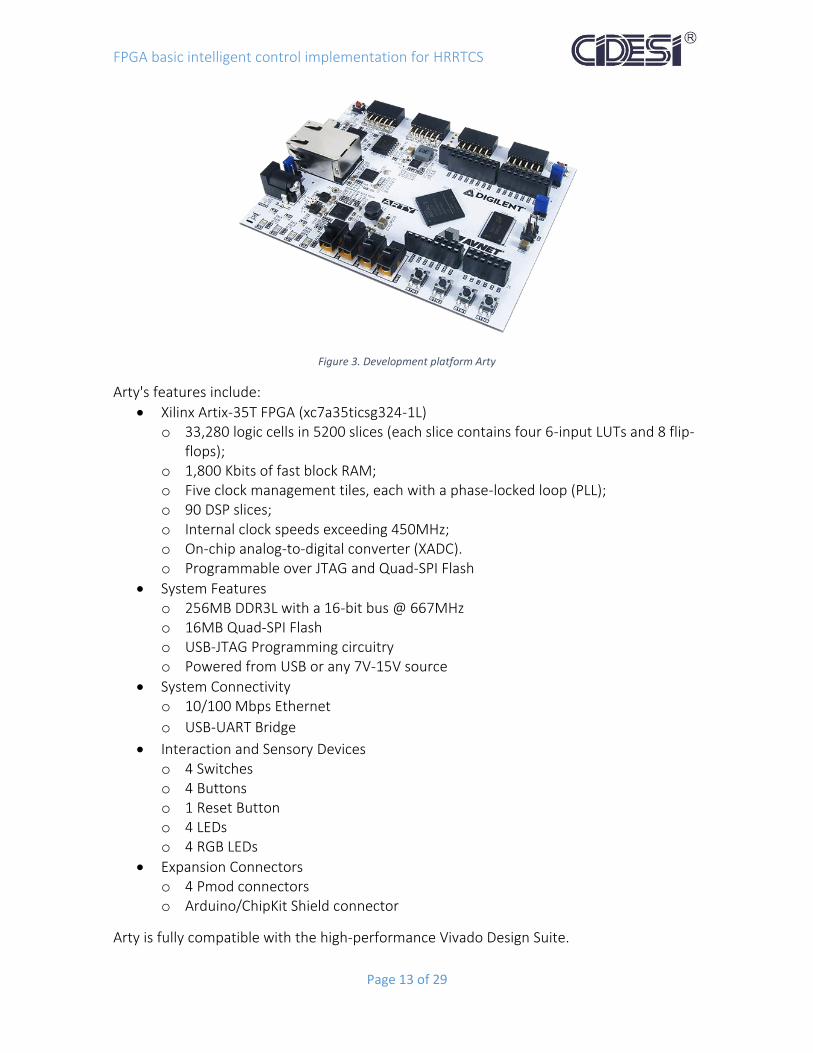
Figure 3. Development platform Arty

Arty's features include:

Xilinx Artix-35T FPGA (xc7a35ticsg324-1L) o 33,280 logic cells in 5200 slices (each slice contains four 6-input LUTs and 8 flip-

flops); o 1,800 Kbits of fast block RAM; o Five clock management tiles, each with a phase-locked loop (PLL); o 90 DSP slices; o Internal clock speeds exceeding 450MHz; o On-chip analog-to-digital converter (XADC). o Programmable over JTAG and Quad-SPI Flash

System Features o 256MB DDR3L with a 16-bit bus @ 667MHz o 16MB Quad-SPI Flash o USB-JTAG Programming circuitry o Powered from USB or any 7V-15V source

System Connectivity o 10/100 Mbps Ethernet

o USB-UART Bridge

Interaction and Sensory Devices o 4 Switches o 4 Buttons o 1 Reset Button o 4 LEDs o 4 RGB LEDs

Expansion Connectors o 4 Pmod connectors o Arduino/ChipKit Shield connector

Arty is fully compatible with the high-performance Vivado Design Suite.


Page 14 of 29

VHDL

VHDL (VHSIC Hardware Description Language) is a hardware description language used in

electronic design automation to describe digital and mixed-signal systems such as field-

programmable gate arrays and integrated circuits. VHDL can also be used as a general

purpose parallel programming language.

Design

VHDL is commonly used to write text models that describe a logic circuit. Such a model is

processed by a synthesis program, only if it is part of the logic design. A simulation program

is used to test the logic design using simulation models to represent the logic circuits that

interface to the design. This collection of simulation models is commonly called a testbench.

VHDL has constructs to handle the parallelism inherent in hardware designs, but these

constructs (processes) differ in syntax from the parallel constructs in Ada (tasks). Like Ada,

VHDL is strongly typed and is not case sensitive. In order to directly represent operations

which are common in hardware, there are many features of VHDL which are not found in

Ada, such as an extended set of Boolean operators including nand and nor. VHDL also allows

arrays to be indexed in either ascending or descending direction; both conventions are used

in hardware, whereas in Ada and most programming languages only ascending indexing is

available.

VHDL has file input and output capabilities, and can be used as a general-purpose language

for text processing, but files are more commonly used by a simulation testbench for stimulus

or verification data. There are some VHDL compilers which build executable binaries. In this

case, it might be possible to use VHDL to write a testbench to verify the functionality of the

design using files on the host computer to define stimuli, to interact with the user, and to

compare results with those expected. However, most designers leave this job to the

simulator.

It is relatively easy for an inexperienced developer to produce code that simulates

successfully but that cannot be synthesized into a real device, or is too large to be practical.

One particular pitfall is the accidental production of transparent latches rather than D-type

flip-flops as storage elements.

One can design hardware in a VHDL IDE (for FPGA implementation such as Xilinx ISE, Altera

Quartus, Synopsys Synplify or Mentor Graphics HDL Designer) to produce the RTL schematic

of the desired circuit. After that, the generated schematic can be verified using simulation

software which shows the waveforms of inputs and outputs of the circuit after generating

the appropriate testbench. To generate an appropriate testbench for a particular circuit or

VHDL code, the inputs have to be defined correctly. For example, for clock input, a loop

process or an iterative statement is required.


Page 15 of 29

A final point is that when a VHDL model is translated into the "gates and wires" that are

mapped onto a programmable logic device such as a CPLD or FPGA, then it is the actual

hardware being configured, rather than the VHDL code being "executed" as if on some form

of a processor chip.

Advantages

The key advantage of VHDL, when used for systems design, is that it allows the behavior of

the required system to be described (modeled) and verified (simulated) before synthesis

tools translate the design into real hardware (gates and wires).

Another benefit is that VHDL allows the description of a concurrent system. VHDL is a

dataflow language, unlike procedural computing languages such as BASIC, C, and assembly

code, which all run sequentially, one instruction at a time.

A VHDL project is multipurpose. Being created once, a calculation block can be used in many

other projects. However, many formational and functional block parameters can be tuned

(capacity parameters, memory size, element base, block composition and interconnection

structure).

A VHDL project is portable. Being created for one element base, a computing device project

can be ported on another element base, for example VLSI with various technologies.

PROJECT DEVELOPMENT To start programming in Vivado Design Suite, the sample programs shown below were

performed.

This program is about an AND gate with two inputs and one output. The explanation of each

instruction code is displayed next.

One of the most used libraries in the world of industry is called ieee, which contains some

types and functions that supplements that come by default in the language itself. Inside the

library there is a package called std_logic_1164, with which you can work with a system of

nine logic levels, such as unknown value, high impedance, etc. It is declared as follows:

library IEEE;

use IEEE.STD_LOGIC_1164.ALL;

The entity is to define the inputs and outputs that have a particular circuit. To define an entity

will be made by the keyword ENTITY. The PORT instruction defines the inputs and outputs of

the defined module. Basically it is to indicate the signal name followed by a colon and the

port address, plus the type of signal that it is. As before, if there is more than one signal it

will end with a semicolon, except the last signal from the list.


Page 16 of 29

entity AND_GATE is Port ( a : in STD_LOGIC; b : in STD_LOGIC; c : out STD_LOGIC); end AND_GATE;

The name of the architecture will be used to indicate what architecture should be used if you have several for the same entity. After this line several instructions may appear to indicate the statement signals, components, functions, etc. These signals are internal, that is, they cannot be accessed from the entity, for which top-level circuits could not access them. In this part of the architecture other elements may also appear, as may be constant. The following is the keyword BEGIN, which leads to the description of the circuit, through a series of sentences. VHDL is a concurrent language, therefore not the order in which the instructions when running the code are written will be followed. In fact, if two instructions need not run one before another, they can run at once. The basic instruction concurrent execution is the allocation between signals through the symbol <=. Therefore, the syntax of architecture is:

architecture Behavioral of AND_GATE is begin c <= a AND b; end Behavioral;

Other programs listed below were designed to improve programming logic in VHDL. The following program is a binary counter with LEDs, it has a clock input and 4 outputs are connected to the LEDs:

library IEEE; use IEEE.STD_LOGIC_1164.ALL; use IEEE.NUMERIC_STD.ALL; library UNISIM; use UNISIM.VComponents.all; entity LedCounter is Port ( clk : in STD_LOGIC; led0_b : out STD_LOGIC; led1_b : out STD_LOGIC; led2_b : out STD_LOGIC; led3_b : out STD_LOGIC); end LedCounter; architecture Behavioral of LedCounter is signal counter : UNSIGNED(28 DOWNTO 0);


Page 17 of 29

begin process (clk) begin -- count from 0 to 2^29-1 and wrap around if (clk'event and clk = '1') then counter <= counter +1; end if; end process; -- connect the 4 MSBs to the blue LEDs led3_b <= counter(28); led2_b <= counter(27); led1_b <= counter(26); led0_b <= counter(25); end Behavioral;

The following program is an adder with four binary inputs, the binary sum converts it for display on a 7-segment display. To find the exit and reduce code in this program Karnaugh maps were made:

library IEEE; use IEEE.STD_LOGIC_1164.ALL; entity bcd is Port ( A : in STD_LOGIC_VECTOR (1 downto 0); C : in STD_LOGIC_VECTOR (1 downto 0); B : out STD_LOGIC_VECTOR (6 downto 0)); end bcd; architecture Behavioral of bcd is signal suma: STD_LOGIC_VECTOR (2 downto 0); begin suma(0) <= A(0) XOR C(0); suma(1) <= (A(1) AND (NOT C(1)) AND (NOT C(0))) OR (A(1) AND (NOT A(0)) AND (NOT C(1))) OR ((NOT A(1)) AND (NOT A(0)) AND C(1)) OR ((NOT A(1)) AND C(1) AND (NOT C(0))) OR ((NOT A(1)) AND A(0) AND (NOT C(1)) AND C(0)) OR (A(1) AND A(0) AND C(1) AND C(0)); suma(2) <= (A(1) AND C(1)) OR (A(0) AND A(1) AND C(0)) OR (C(1) AND C(0) AND A(0)); with suma select B <= "1000000" when "000", "1111001" when "001", "0100100" when "010", "0110000" when "011", "0011001" when "100",


Page 18 of 29

"0010010" when "101", "0000010" when "110", "1111111" when others; end Behavioral;

IMPLEMENTATION OF PERCEPTRONS Neural networks can be used to determine relationships and patterns between inputs and outputs. A simple single layer feed forward neural network which has a to ability to learn and differentiate data sets is known as a perceptron. By iteratively “learning” the weights, it is possible for the perceptron to find a solution to linearly separable data (data that can be separated by a hyperplane). In this example made by MATLAB, it was run a simple perceptron to determine the solution to a 2-input OR. X1 or X2 were defined as follows:

Figure 4 Inputs and output of OR gate.

They were first initialized the variables of interest, including the input, desired output, bias, learning coefficient and weights.

input = [0 0; 0 1; 1 0; 1 1]; numIn = 4; desired_out = [0;1;1;1]; bias = -1; coeff = 0.7; rand('state',sum(100*clock)); weights = -1*2.*rand(3,1);

The input and desired_out were self explanatory, with the bias initialized to a constant. This value can be set to any non-zero number between -1 and 1. The coeff represents the learning rate, which specifies how large of an adjustment is made to the network weights after each iteration. If the coefficient approaches 1, the weight adjustments are modified more conservatively. Finally, the weights are randomly assigned.


Page 19 of 29

A perceptron is defined by the equation:

Therefore, in the example, the equation is: w1*x1+w2*x2+b = out It was assumed that weights(1,1) is for the bias and weights(2:3,1) are for X1 and X2, respectively. One more variable was set, specifying how many times to train or go through and modify the weights.

iterations = 10; Now the feed forward perceptron code.

for i = 1:iterations out = zeros(4,1); for j = 1:numIn y = bias*weights(1,1)+... input(j,1)*weights(2,1)+input(j,2)*weights(3,1); out(j) = 1/(1+exp(-y)); delta = desired_out(j)-out(j); weights(1,1) = weights(1,1)+coeff*bias*delta; weights(2,1) = weights(2,1)+coeff*input(j,1)*delta; weights(3,1) = weights(3,1)+coeff*input(j,2)*delta; end end

A little explanation of the code. First, the equation solving for ‘out’ was determined as mentioned above, and then run through a sigmoid function to ensure values were squashed within a [0 1] limit. Weights were then modified iteratively based on the delta rule. When running the perceptron over 10 iterations, the outputs began to converge, but were still not precisely as expected:

out = 0.3756 0.8596 0.9244 0.9952 weights = 0.6166 3.2359 2.7409


Page 20 of 29

As the iterations approach 1000, the output converged towards the desired output. out = 0.0043 0.9984 0.9987 1.0000 weights = 5.4423 12.1084 11.8823

The next step was to try to pass this code to VHDL. It was reached following code, however some compilation errors were obtained, because the VHDL language does not allow the creation of vectors of real numbers. The code was as follows:

library IEEE; use IEEE.STD_LOGIC_1164.ALL; use IEEE.NUMERIC_STD.ALL; library UNISIM; use UNISIM.VComponents.all; entity perceptron_final is Port (); end perceptron_final; architecture Behavioral of perceptron_final is signal x1 : bit_vector(3 downto 0) ; signal x2 : bit_vector(3 downto 0) ; signal d : bit_vector(3 downto 0) ; begin x1(0) <= '0'; x1(1) <= '0'; x1(2) <= '1'; x1(3) <= '1'; x2(0) <= '0'; x2(1) <= '1'; x2(2) <= '0'; x2(3) <= '1'; d(0) <= '0'; d(1) <= '1'; d(2) <= '1'; d(3) <= '1';


Page 21 of 29

process variable w0: real :=0.5; variable w1: real :=0.5; variable w2: real :=0.5; variable suma: real :=0.5; variable error: real; variable y: std_logic; constant a: real :=1.0; constant x0: real :=1.0; begin bucle1: FOR i IN 0 TO 3 LOOP suma := x1(i)*w1 + x2(i)*w2 + x0*w0; if (suma>=0.0) then y :='1'; else y :='0'; error := d(i)-y; if(error/=0.0)then w0 := w0 + a*error*x0; w1 := w1 + a*error*x1(i); w2 := w2 + a*error*x2(i); else w0=w0; end if; end if; END LOOP bucle1; end process; end Behavioral;

Because it was failed to obtain the weights in VHDL, they were obtained analytically, and to prove that these weights were correct the following codes test were conducted, where the equation of the boundary decision perceptron was written, and with input switches this equation was tested, taking a LED as output: The implemented code to the AND gate is shown with two inputs connected to switches, and output to a LED. Because VHDL cannot run programs on the card with real numbers (only in simulation), weights were multiplied by a factor of 10 to have only integer numbers.

library IEEE;a


Page 22 of 29

use IEEE.STD_LOGIC_1164.ALL; use IEEE.NUMERIC_STD.ALL; library UNISIM; use UNISIM.VComponents.all; entity perceptron2 is Port ( output : out STD_LOGIC; input1 : in STD_LOGIC_VECTOR(0 DOWNTO 0); input0 : in STD_LOGIC_VECTOR(0 DOWNTO 0)); end perceptron2; architecture Behavioral of perceptron2 is signal a : integer; signal b : integer; signal threshold : integer := 10; begin b <= to_integer(unsigned(input1)); a <= to_integer(unsigned(input0)); process(threshold, a, b) variable activation : integer := 0; variable peso1 : integer := 6; variable peso2 : integer := 6; begin activation := a*peso1 + b*peso2; if(activation>=threshold) then output <= '1'; else output <= '0'; end if; end process; end Behavioral;

To make the OR gate, the code of the AND gate only changed in the value of the weights:

library IEEE; use IEEE.STD_LOGIC_1164.ALL; use IEEE.NUMERIC_STD.ALL; library UNISIM; use UNISIM.VComponents.all;


Page 23 of 29

entity perceptron2 is Port ( output : out STD_LOGIC; input1 : in STD_LOGIC_VECTOR(0 DOWNTO 0); input0 : in STD_LOGIC_VECTOR(0 DOWNTO 0)); end perceptron2; architecture Behavioral of perceptron2 is signal a : integer; signal b : integer; signal threshold : integer := 10; begin b <= to_integer(unsigned(input1)); a <= to_integer(unsigned(input0)); process(threshold, a, b) variable activation : integer := 0; variable peso1 : integer := 11; variable peso2 : integer := 11; begin activation := a*peso1 + b*peso2; if(activation>=threshold) then output <= '1'; else output <= '0'; end if; end process; end Behavioral;

The following code design shows a NOT gate, which only took one input and one output:

library IEEE; use IEEE.STD_LOGIC_1164.ALL; use IEEE.NUMERIC_STD.ALL; library UNISIM; use UNISIM.VComponents.all; entity perceptron2 is Port ( output : out STD_LOGIC; input0 : in STD_LOGIC_VECTOR(0 DOWNTO 0));


Page 24 of 29

end perceptron2; architecture Behavioral of perceptron2 is signal a : integer; signal threshold : integer := -5; begin a <= to_integer(unsigned(input0)); process(threshold, a ) variable activation : integer := 0; variable peso1 : integer := -10; begin activation := a*peso1 ; if(activation>=threshold) then output <= '1'; else output <= '0'; end if; end process; end Behavioral;

In the following program, it was developed an XOR gate design, this design was more complicated, because three neurons for implementation were needed unlike the others only occupied one neuron:

library IEEE; use IEEE.STD_LOGIC_1164.ALL; use IEEE.NUMERIC_STD.ALL; library UNISIM; use UNISIM.VComponents.all; entity perceptron2 is Port ( output : out STD_LOGIC; input1 : in STD_LOGIC_VECTOR(0 DOWNTO 0); input0 : in STD_LOGIC_VECTOR(0 DOWNTO 0)); end perceptron2; architecture Behavioral of perceptron2 is signal a : integer; signal b : integer;


Page 25 of 29

signal threshold : integer := 10; begin b <= to_integer(unsigned(input1)); a <= to_integer(unsigned(input0)); process(a, b) variable activation1 : integer := 0; variable peso1 : integer := 6; variable peso2 : integer := 6; variable out1 : integer; variable activation2 : integer := 0; variable peso3 : integer := 11; variable peso4 : integer := 11; variable out2 : integer; variable activation : integer := 0; variable peso5 : integer := -20; variable peso6 : integer := 11; begin activation1 := a*peso1 + b*peso2; if(activation1>=threshold) then out1 := 1; else out1 := 0; end if; activation2 := a*peso3 + b*peso4; if(activation2>=threshold) then out2 := 1; else out2 := 0; end if; activation := out1*peso5 + out2*peso6; if(activation>=threshold) then output <= '1'; else output <= '0'; end if; end process;


Page 26 of 29

end Behavioral;

RESULTS The results obtained are shown for some of the codes implemented in VHDL.

In the next picture the simulation of the first code is shown, the variation of the inputs with

the time and the output of an AND gate, are shown:

Figure 5 Simulation of the first simple code.

In the next picture, it is shown the implementation of the counter leds code deployed on

the ARTY, it is noted the change on the lighting on the leds depending on time:

Figure 6 Implementation of the Sample “Led counter program”.


Page 27 of 29

In the next picture, it is shown the ARTY with one of the codes of the perceptron

implemented.

The implementation of the code for an OR gate perceptron is shown next, it was tested with

two inputs whose values changed from 00, 01, 10 and 11 at press the switches, and the

output took the values of 0,1,1,1.

Figure 7 OR gate perceptron.

The other codes of the AND, NOT and XOR gate perceptrons were also implemented in the

ARTY, and also had the expected results.

The only code that couldn’t work, is the code for calculating the weights of the neuron in

VHDL, the problem was that at the moment of the creation of the input arrays, it couldn’t be

implemented the arithmetic operations for the type of signal, it was STD_LOGIC_VECTOR

and when it was converted to REAL, it was converter to a single number instead of an array.

Therefore, the pseudocode known for calculating the weights of a perceptron is not feasible

and it should be looked for another way, because the programming on an FPGA is parallel

and it should be taken advantage of this quality.

It is expected to find the solution of the mistakes soon and improve this project.

CONCLUSION This project was started with an intensive learning stage by its executer (E. González). Basics

for Artificial Neural Networks (ANN) and Vivado software were quickly learned. It was begun

reading different websites where the basic concepts of artificial neural networks were

explained, it was seen a tutorial on YouTube about this topic and exercises were conducted


Page 28 of 29

in the notebook to better understand the concept of perceptron. A software problem was

solved concerning the compatibility between the operating system and Vivado.

The development process was as follows. Having installed the software, tutorials were seen

to learn how to program in Vivado with examples in Verilog and VHDL, some of the examples

are shown in this report. It was implemented a successful program to calculate the weights

for the ANN in MATLAB. The weights were calculated analytically, and to check that they

were correct, they were created some codes in VHDL with the equation of the perceptron,

switches as inputs and a led as output.

This was a complex project were several issues still open, as the weights calculations of the

ANN through the software Vivado. Finally, it is concluded that this is a fascinating subject and

we would like to go further into it.

ACKNOWLEDGMENTS I would like to thank all the personnel of CIDESI especially Dr. Gengis K. Toledo Ramirez, for

accepting me in the program and for all support, Dr. Jose Antonio Torres Estrada and M.I.

Jonatan Marcelo Sosa Rincón, the person who helped me in doubts of VHDL programming. I

also would like to thank the Dolphin Program, through whom I had the opportunity to live

this very enriching experience, the Technological Institute of Morelia, for supporting me with

resource so that it could be possible to make this stay, I finally want to thank my fellows

Carolina Soria Zapata and Manuel Estrada Angulo for sharing this experience with me and to

my family for always supporting me.

REFERENCES

DIGILENT. “Arty Reference Manual.” Internet:

https://reference.digilentinc.com/reference/programmable-logic/arty/reference-manual,

[July 27, 2016].

Hackeando Tec. “Curso de Redes Neuronales Artificiales.” Internet:

https://www.youtube.com/watch?v=14tU9B4ReII&list=PLIyIZGa1sAZo_eY8PpuTxfLsja_iyytE

[July 27, 2016].

W. McCulloch and W. Pitts. "A Logical Calculus of Ideas Immanent in Nervous

Activity." Bulletin of Mathematical Biophysics, 19435, pp. 115–133.

Y. Freund and R. Schapire. "Large margin classification using the perceptron

algorithm" Machine Learning, 1999, 277–296.

https://reference.digilentinc.com/reference/programmable-logic/arty/reference-manual

https://www.youtube.com/channel/UCCFT304Nz5pSWktsiidUy0Q

https://www.youtube.com/watch?v=14tU9B4ReII&list=PLIyIZGa1sAZo_eY8PpuTxfLsja_iyytE

https://en.wikipedia.org/wiki/Robert_Schapire

http://cseweb.ucsd.edu/~yfreund/papers/LargeMarginsUsingPerceptron.pdf

http://cseweb.ucsd.edu/~yfreund/papers/LargeMarginsUsingPerceptron.pdf

https://en.wikipedia.org/wiki/Machine_Learning_(journal)


Page 29 of 29

C. Bishop. Pattern Recognition and Machine Learning. N.Y: Springe, 2007, pp. 120-130.

V. Lugade. “Neural Networks – A perceptron in Matlab.” Internet:

http://matlabgeeks.com/tips-tutorials/neural-networks-a-perceptron-in-matlab/, May 11, 2011

[July 30, 2016].

http://matlabgeeks.com/tips-tutorials/neural-networks-a-perceptron-in-matlab/

FPGA ASI INTELLIGENT ONTROL IMPLEMENTATION FOR … · FPGA basic intelligent ... through the...

Documents

Transcript of FPGA ASI INTELLIGENT ONTROL IMPLEMENTATION FOR … · FPGA basic intelligent ... through the...