Fourier Transform (Continuous- Time)• Periodic signals can be represented as

linear combinations of harmonicallyrelated complex exponentials.

• To extend this to non-periodic signals,consider aperiodic signals as periodicsignals with infinite period.

∑∑∞

−∞=

∞

−∞=

==k

tTjkk

k

tjkk eaeatx )/2(0)( πω

𝑎𝑎𝑘𝑘 =1𝑇𝑇�0

𝑇𝑇𝑥𝑥(𝑡𝑡)𝑒𝑒−𝑗𝑗𝑘𝑘𝜔𝜔0𝑡𝑡𝑑𝑑𝑡𝑡

where

𝑎𝑎𝑘𝑘 =1𝑇𝑇�0

𝑇𝑇𝑥𝑥(𝑡𝑡)𝑒𝑒−𝑗𝑗𝑘𝑘𝜔𝜔0𝑡𝑡𝑑𝑑𝑡𝑡 =

2sin(𝑘𝑘𝜔𝜔0𝑇𝑇𝑝𝑝)𝑘𝑘𝜔𝜔0𝑇𝑇

𝑥𝑥 𝑡𝑡 =1, |𝑡𝑡| ≤ 𝑇𝑇𝑝𝑝0, 𝑇𝑇𝑝𝑝< 𝑡𝑡 < 𝑇𝑇/2

𝑇𝑇𝑎𝑎𝑘𝑘 =2sin(𝜔𝜔𝑇𝑇𝑝𝑝)

𝜔𝜔𝜔𝜔 = 𝑘𝑘𝜔𝜔0

As the period becomes infinite, instead of using the coefficients, we’ll now look

at the Fourier transform which is a complex valued function in the

frequency domain.

𝑇𝑇𝑎𝑎𝑘𝑘 =2sin(𝜔𝜔𝑇𝑇𝑝𝑝)

𝜔𝜔

Perio

d in

crea

ses

𝑇𝑇𝑎𝑎𝑘𝑘 = �−𝑇𝑇/2

𝑇𝑇/2𝑥𝑥(𝑡𝑡)𝑒𝑒−𝑗𝑗𝑘𝑘𝜔𝜔0𝑡𝑡𝑑𝑑𝑡𝑡 =?

* As the period goes to infinity,

𝜔𝜔 = 𝑘𝑘𝜔𝜔0

Definition of the Fourier Transform

• For any signal x(t), the Fourier transform synthesis describes its Fourier transform X(jω)

and the analysis equations (inverse Fourier transform) is given as

• We will refer to x(t) and X(jω) as a Fourier transform pair with the notation

𝑥𝑥(𝑡𝑡) =12𝜋𝜋

�−∞

∞𝑋𝑋(𝑗𝑗𝜔𝜔)𝑒𝑒𝑗𝑗𝜔𝜔𝑡𝑡𝑑𝑑𝜔𝜔 = 𝐹𝐹−1{𝑋𝑋(𝑗𝑗𝜔𝜔)}

𝑋𝑋(𝑗𝑗𝜔𝜔) = �−∞

∞𝑥𝑥(𝑡𝑡)𝑒𝑒−𝑗𝑗𝜔𝜔𝑡𝑡𝑑𝑑𝑡𝑡 = 𝐹𝐹{𝑥𝑥(𝑡𝑡)}

)()( ωjXtxF

↔

Example: • Consider the (non-periodic) signal

• Then the Fourier transform is:

5/16

𝑥𝑥(𝑡𝑡) = 𝑒𝑒−𝑡𝑡𝑢𝑢(𝑡𝑡)

= �−∞

∞𝑒𝑒−𝑡𝑡𝑢𝑢 𝑡𝑡 𝑒𝑒−𝑗𝑗𝜔𝜔𝑡𝑡𝑑𝑑𝑡𝑡

= �0

∞𝑒𝑒−(1+𝑗𝑗𝜔𝜔)𝑡𝑡𝑑𝑑𝑡𝑡

= �1

−(1 + 𝑗𝑗𝜔𝜔)𝑒𝑒−(1+𝑗𝑗𝜔𝜔)𝑡𝑡

0

∞

=1

(1 + 𝑗𝑗𝜔𝜔)

𝑋𝑋 𝑗𝑗𝜔𝜔

Example:• Consider the non-periodic rectangular pulse at zero

• The Fourier transform is:

𝑥𝑥(𝑡𝑡) = �1 |𝑡𝑡| < 10 |𝑡𝑡| ≥ 1

𝑋𝑋 𝑗𝑗𝜔𝜔 = �−∞

∞𝑥𝑥 𝑡𝑡 𝑒𝑒−𝑗𝑗𝜔𝜔𝑡𝑡𝑑𝑑𝑡𝑡 =

2 sin(𝜔𝜔)𝜔𝜔

Example:• Consider the signal x(t) whose Fourier transform is

• Then, the inverse Fourier transform is:

X(𝑗𝑗𝜔𝜔) = �1 |𝜔𝜔| < 10 |𝜔𝜔| ≥ 1

𝑥𝑥 𝑡𝑡 =1

2π�−1

1𝑋𝑋 𝑗𝑗𝜔𝜔 𝑒𝑒𝑗𝑗𝜔𝜔𝑡𝑡𝑑𝑑𝜔𝜔 =

sin( 𝑡𝑡)π𝑡𝑡

Exercises:1) Use the Fourier transform analysis equation to calculate the Fourier transforms of

2) Use the Fourier transform synthesis equation to determine the inverse Fourier transform of

where

𝑎𝑎) 𝑥𝑥 𝑡𝑡 = 𝑒𝑒−4 𝑡𝑡−1 𝑢𝑢(𝑡𝑡 − 1) 𝑏𝑏) 𝑥𝑥 𝑡𝑡 = 𝛿𝛿 𝑡𝑡 + 1 + 𝛿𝛿(𝑡𝑡 − 1)

𝑋𝑋 𝑗𝑗ω = |𝑋𝑋(𝑗𝑗ω)|𝑒𝑒𝑗𝑗<𝑋𝑋(𝑗𝑗ω)

|𝑋𝑋 𝑗𝑗ω | = 2{𝑢𝑢 ω + 3 − 𝑢𝑢 ω − 3 }

< 𝑋𝑋 𝑗𝑗ω = −32

ω + 𝜋𝜋

Impulse Signal• The Fourier transform of the impulse signal can be calculated as follows:

• Therefore, the Fourier transform of the impulse function has a constant contribution for all frequencies.

1)()(

)()(

==

=

∫∞

∞−

− dtetjX

ttxtjωδω

δ

ω

X(jω) 𝑥𝑥(𝑡𝑡) = 𝛿𝛿(𝑡𝑡 − 4)

𝑋𝑋 𝑗𝑗𝜔𝜔 = �−∞

∞𝛿𝛿 𝑡𝑡 − 4 𝑒𝑒−𝑗𝑗𝜔𝜔𝑡𝑡𝑑𝑑𝑡𝑡 =?

• For periodic signals,

• Then, the corresponding Fourier transform is given as

• The Fourier transform of a periodic signal is a train of impulses at the harmonic frequencies with amplitude 2πak.

∑∞

−∞=

−=k

k kajX )(2)( 0ωωδπω

∑∞

−∞=

=k

tjkkeatx 0)( ω

2π𝛿𝛿 𝜔𝜔 − 𝑘𝑘𝜔𝜔0 𝑒𝑒𝑗𝑗𝑘𝑘𝜔𝜔0𝑡𝑡

Exercises:

Determine the Fourier transforms of

𝑎𝑎) 𝑥𝑥 𝑡𝑡 = sin(ω0𝑡𝑡)

𝑏𝑏) 𝑥𝑥 𝑡𝑡 = 1.5, 0 ≤ 𝑡𝑡 ≤ 1−1.5, 1 ≤ 𝑡𝑡 ≤ 2 Periodic CT signal with fundamental frequency ω0 =π.

Linearity of the Fourier Transform

• If and

then

13/14

)()( ωjXtxF

↔ )()( ωjYtyF

↔

)()()()( ωω jbYjaXtbytaxF

+↔+

Linearity

• If

then

A signal which is shifted in time does not have its Fourier transform magnitude altered, only a shift in phase.

)()( ωjXtxF

↔

)()( 00 ωω jXettx tj

F−↔−

)()}({ 00 ωω jXettxF tj−=−

Translation (Time-Domain Shifting)

Modulation (Frequency-Domain Shifting)

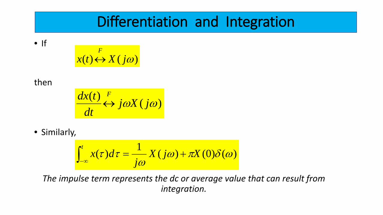
Differentiation and Integration• If

then

• Similarly,

The impulse term represents the dc or average value that can result from integration.

)()( ωω jXjdt

tdx F↔

)()0()(1)( ωδπωω

ττ XjXj

dxt

+=∫ ∞−

)()( ωjXtxF

↔

Convolution in the Frequency Domain

• With a bit of work (next slide) it can show that:

• Therefore, to apply convolution in the frequency domain, we just have to multiply the two functions.

• To solve for the differential/convolution equation using Fourier transforms:1. Calculate Fourier transforms of x(t) and h(t)2. Multiply H(jω) by X(jω) to obtain Y(jω)3. Calculate the inverse Fourier transform of Y(jω)

• Multiplication in the frequency domain corresponds to convolution in the time domain and vice versa.

)()()()(*)()( ωωω jXjHjYtxthtyF

=↔=

Convolution

Properties of Fourier Transform (CT)

Fourier Transform Pairs (CT)

Example:• Consider the signal (linear sum of two time shifted steps)

where x1(t) is of width 1, x2(t) is of width 3, centred on zero.

• Using the rectangular pulse example

• Then, using the linearity and time shift Fourier transform properties

)5.2()5.2(5.0)( 21 −+−= txtxtx

( )

+= −

ωωωω ω )2/3sin(2)2/sin()( 2/5jejX

Exercises:1) Express the Fourier transforms of the signals listed below in terms of X(jω).

2) Determine x(t) given the Fourier transform of

𝑎𝑎) 𝑥𝑥 𝑡𝑡 = 𝑥𝑥 𝑡𝑡 − 1 + 𝑥𝑥 𝑡𝑡 + 1

𝑏𝑏) 𝑥𝑥 𝑡𝑡 =𝑑𝑑2

𝑑𝑑𝑡𝑡2𝑥𝑥 𝑡𝑡 − 1

𝑋𝑋 𝑗𝑗𝑗𝑗 =1

6 + 𝑗𝑗𝑗𝜔𝜔 − 𝜔𝜔2

Exercises:3) Consider a causal LTI system with frequency response

For a particular input x(t) this system is observed to produce the output:

Determine x(t).

𝐻𝐻 𝑖𝑖ω =1

𝑗𝑗ω + 3

y 𝑡𝑡 = 𝑒𝑒−3𝑡𝑡𝑢𝑢 𝑡𝑡 − 𝑒𝑒−4𝑡𝑡𝑢𝑢 𝑡𝑡

Summary: Fourier Transform (CT)

• CT Fourier transform maps a time domain frequency signal to the

frequency domain via

• The Fourier transform is used to

• analyse the frequency content of a signal

• design a system/filter with particular properties

• solve differential equations in the frequency domain using algebraic operators

∫∫

∞

∞−

−

∞

∞−

=

=

dtetxjX

dejXtx

tj

tj

ω

ωπ

ω

ωω

)()(

)()( 21

Summary: Fourier Series (Discrete Time )• The closed form expression for the discrete time Fourier series

coefficients are given as

• 𝑎𝑎𝑘𝑘 are the spectral coefficients of x[n].• Since there are only N distinct harmonically related signals in

discrete-time signals, the summation include terms over this range.

x[n] = �𝑘𝑘=<𝑁𝑁>

𝑎𝑎𝑘𝑘𝑒𝑒𝑗𝑗𝑘𝑘𝜔𝜔0𝑛𝑛

where

𝑎𝑎𝑘𝑘=1𝑁𝑁

�𝑘𝑘=<𝑁𝑁>

𝑥𝑥[𝑛𝑛]𝑒𝑒−𝑗𝑗𝑘𝑘𝜔𝜔0𝑛𝑛

𝑥𝑥(𝑡𝑡) = �𝑘𝑘=−∞

∞

𝑎𝑎𝑘𝑘𝑒𝑒𝑗𝑗𝑘𝑘𝜔𝜔0𝑡𝑡

∫ −=T tjn

Tn dtetxa0

1 0)( ω

CTFourier Series

DTFourier Series

Fourier Transform (Discrete Time )• The DT Fourier transform synthesis and analysis equations are

therefore:

• The function X(ejω) is referred to as the discrete-time Fouriertransform and the pair of equations are referred to as the Fouriertransform pair.

𝑥𝑥[𝑛𝑛] =12𝜋𝜋

�2𝜋𝜋𝑋𝑋(𝑒𝑒𝑗𝑗𝜔𝜔)𝑒𝑒𝑗𝑗𝜔𝜔𝑛𝑛𝑑𝑑𝜔𝜔

where

𝑋𝑋(𝑒𝑒𝑗𝑗𝜔𝜔) = �𝑛𝑛=−∞

∞

𝑥𝑥[𝑛𝑛]𝑒𝑒−𝑗𝑗𝜔𝜔𝑛𝑛

x[n] = �𝑘𝑘=<𝑁𝑁>

𝑎𝑎𝑘𝑘𝑒𝑒𝑗𝑗𝑘𝑘𝜔𝜔0𝑛𝑛

where

𝑎𝑎𝑘𝑘=1𝑁𝑁

�𝑘𝑘=<𝑁𝑁>

𝑥𝑥[𝑛𝑛]𝑒𝑒−𝑗𝑗𝑘𝑘𝜔𝜔0𝑛𝑛

DTPeriodicDT

Aperiodic

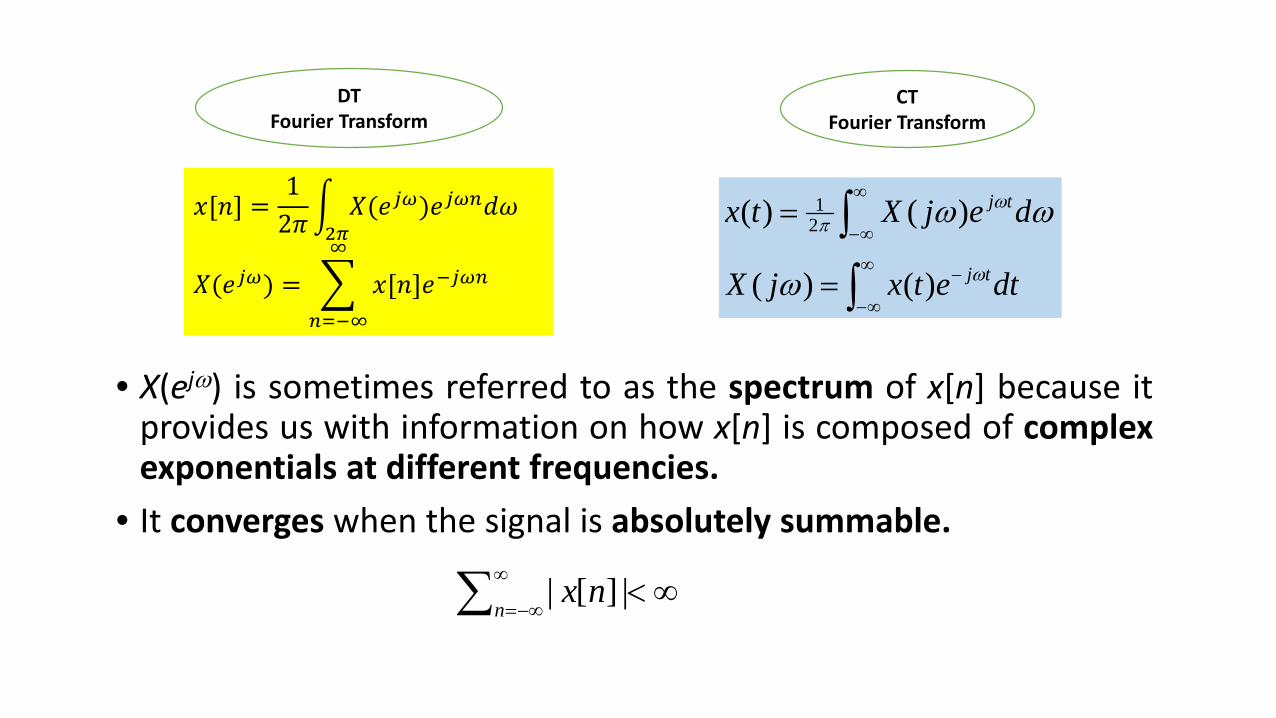
• X(ejω) is sometimes referred to as the spectrum of x[n] because itprovides us with information on how x[n] is composed of complexexponentials at different frequencies.

• It converges when the signal is absolutely summable.

∑∞

−∞=∞<

nnx |][|

∫∫

∞

∞−

−

∞

∞−

=

=

dtetxjX

dejXtx

tj

tj

ω

ωπ

ω

ωω

)()(

)()( 21

CTFourier Transform

DTFourier Transform

𝑥𝑥[𝑛𝑛] =12𝜋𝜋

�2𝜋𝜋𝑋𝑋(𝑒𝑒𝑗𝑗𝜔𝜔)𝑒𝑒𝑗𝑗𝜔𝜔𝑛𝑛𝑑𝑑𝜔𝜔

𝑋𝑋(𝑒𝑒𝑗𝑗𝜔𝜔) = �𝑛𝑛=−∞

∞

𝑥𝑥[𝑛𝑛]𝑒𝑒−𝑗𝑗𝜔𝜔𝑛𝑛

Examples:

• Calculate the DT Fourier transform of the following signals:

i)

ii)

iii)

𝑥𝑥[𝑛𝑛] = 𝑎𝑎𝑛𝑛𝑢𝑢[𝑛𝑛], |𝑎𝑎| < 1

ωω

ωω

jn

nj

n

njnj

aeae

enuaeX

−

∞

=

−

∞

−∞=

−

−==

=

∑

∑

11)(

][)(

0

𝑥𝑥[𝑛𝑛] = 𝑎𝑎|𝑛𝑛|, |𝑎𝑎| < 1

𝑥𝑥[𝑛𝑛] = 1, |𝑛𝑛| ≤ 𝑁𝑁𝑁0, |𝑛𝑛| > 𝑁𝑁𝑁

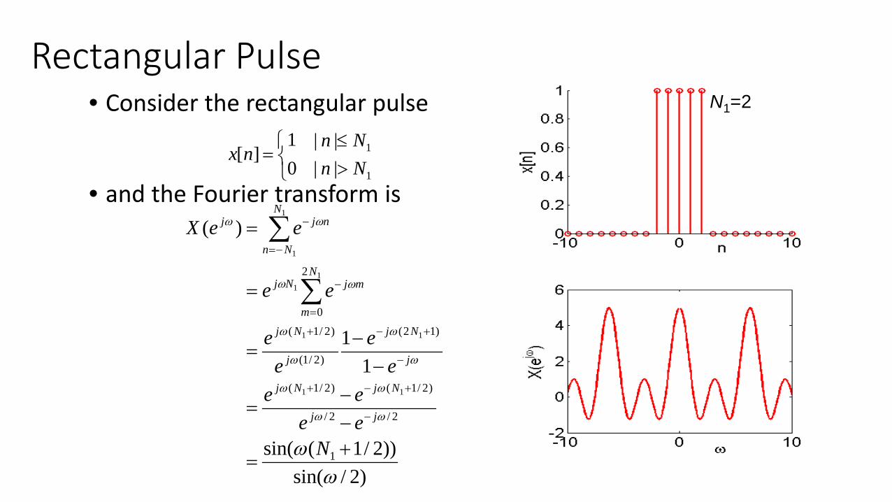
Rectangular Pulse• Consider the rectangular pulse

• and the Fourier transform is

>≤

=1

1

||0||1

][NnNn

nx

)2/sin())2/1(sin(

11

)(

1

2/2/

)2/1()2/1(

)12(

)2/1(

)2/1(

2

0

11

11

11

1

1

ωω

ωω

ωω

ω

ω

ω

ω

ωω

ωω

+=

−−

=

−−

=

=

=

−

+−+

−

+−+

=

−

−=

−

∑

∑

Neeee

ee

ee

ee

eeX

jj

NjNj

j

Nj

j

Nj

N

m

mjNj

N

Nn

njj

N1=2

Properties: Periodicity, Linearity & Time• The DT Fourier transform is always periodic with period 2π, because

X(ej(ω+2π)) = X(ejω)

• It is relatively straightforward to prove that the DT Fourier transform is linear, i.e.

• Similarly, if a DT signal is shifted by n0 units of time

)()(][][

)(][),(][

2121

2211

ωω

ωω

jjF

jF

jF

ebXeaXnbxnax

eXnxeXnx

+↔+

↔↔

)(][

)(][

00

ωω

ω

jnjF

jF

eXennx

eXnx−↔−

↔

Convolution in the Frequency Domain• The time-domain convolution of two discrete time signals

can be represented as the multiplication of the Fouriertransforms.

• If x[n], h[n] and y[n] are the input, impulse response andoutput of a discrete-time LTI system so, by convolution,

y[n] = x[n]*h[n]then

Y(ejω) = X(ejω)H(ejω)

• Convolution in the discrete time domain is replaced bymultiplication in the frequency domain.

Example• Consider an LTI system with impulse response h[n]=αn u[n] where

|α|< 1, and the system input is x[n]=β n u[n] where |β|< 1.• The DT Fourier transforms are:

• So

• Expressing as partial fractions, assuming α ≠ β:

and spotting the inverse Fourier transform

ωω

ωω

βα jj

jj

eeX

eeH −− −

=−

=1

1)(,1

1)(

)1)(1(1)( ωω

ω

βα jjj

eeeY −− −−

=

)1(1

)1(1)( ωω

ω

ββαβ

αβαα

jjj

eeeY −− −−

−−−

=

βαβ

βαα

−−

−=

++ ][][][11 nununy

nn

Exercise

1) Calculate the Fourier transforms of

2) Determine the inverse Fourier transform for

𝑏𝑏) 𝑥𝑥 𝑛𝑛 = 𝛿𝛿 𝑛𝑛 − 1 + 𝛿𝛿 𝑛𝑛 + 1

𝑎𝑎) 𝑥𝑥 𝑛𝑛 = 0.5𝑛𝑛𝑢𝑢 𝑛𝑛 − 1

a) 𝑋𝑋(𝑗𝑗ω) = 2𝑗𝑗, 0 < ω < π−2𝑗𝑗 − π < ω < 0

b) 𝑋𝑋(𝑗𝑗ω) = 𝑒𝑒−𝑗𝑗𝜔𝜔/2 − π ≤ ω ≤ π

Exercise

3) Using FT properties, calculate the Fourier transforms of

4) Consider a discrete-time LTI system with

Use Fourier transforms to determine the response of

𝑥𝑥 𝑛𝑛 = sinπ2𝑛𝑛 + cos(𝑛𝑛) ,

ℎ 𝑛𝑛 = 0.5𝑛𝑛𝑢𝑢 𝑛𝑛𝑥𝑥 𝑛𝑛 = 0.25𝑛𝑛𝑢𝑢 𝑛𝑛 .