Continuous-time Fourier Transform (CTFT) of aperiodic and...

Chap 4 Continuous-time Fourier Transform (CTFT) of aperiodic and periodic signals 1 | P a g e

4

Continuous-time Fourier Transform (CTFT) of aperiodic and periodic

signals

In previous chapters we discussed the Fourier series as it applies to the representation of continuous and discrete signals. We discussed the concept of harmonic sinusoids as basis functions, first the trigonometric version of sinusoids and then the complex exponentials as a more compact form for representing a signal. The analysis signal is “projected” on to these basis signals, and the “quantity” of each basis function is interpreted as spectral content along a frequency line. The main idea is to develop a spectrum of the signal so a qualitative assessment of the signal can be made. Fourier coefficients are one name for spectral content and the whole picture as a function of frequency is called the spectrum. The spectrum has in fact many names in literature such as: bode plots, gain curve, frequency response, rejection, magnitude, power spectrum, power spectral density etc. They are all referring to the distribution of spectral content over a range of frequencies. Fourier series discussions assume that the signal of interest is periodic. But a majority of signals we encounter in signal processing are not periodic. Even those that we think are periodic are not really so. Then we have many signals which are bunch of random bits with no pretense of periodicity. This is the real world of signals and Fourier series comes up short for these types of signals. This was of course noticed right away by the contemporaries of Fourier when he first published his ideas is 1822. Fourier series is great for periodic signals but how about stand-alone non-periodic, also called aperiodic signals like this one?

Figure 4.1 – Can we compute the Fourier series coefficients of this aperiodic signal?

Taking some liberty with history, Fourier, I am sure was disappointed when he received a very unenthusiastic response to his work upon first publishing it. He was denied membership into the French Academy as the work was not considered rigorous enough. His friends and foes, who are now as famous as he is, (Laplace, Lagrange etc.) objected to his overreaching original conclusion about the Fourier series, that it can represent any signal. They correctly guessed that series representation would not work universally, such as for exponential signals as well as for a large class of signals that are not periodic. Baron Fourier, disappointed but not discouraged, came back 20 years later with something even better, the Fourier transform. (If you are having a little bit of difficulty understanding all this on first reading, this is forgivable. Even Fourier took 20 years to develop it.) Extending the period to infinity

In this chapter we will look at the mathematical trick Fourier used to modify the Fourier series such that it could be applied to signals that are not strictly periodic, or are transient. Take the signal in Fig. 4.1. Let’s say that some data has been collected and the data shows no periodicity. Being engineers, we want to compute its spectrum using Fourier analysis, even though we have been told that the signal must be periodic. What to do? Well, we can assume that the signal in Fig. 4.1 is actually a repeating signal and we are only seeing one period. In Figure 4.2(a) we show this signal repeating with a period of 8 samples. Of course, we just made up that period. We truly have no idea what the period of this signal is, or if it even has one.


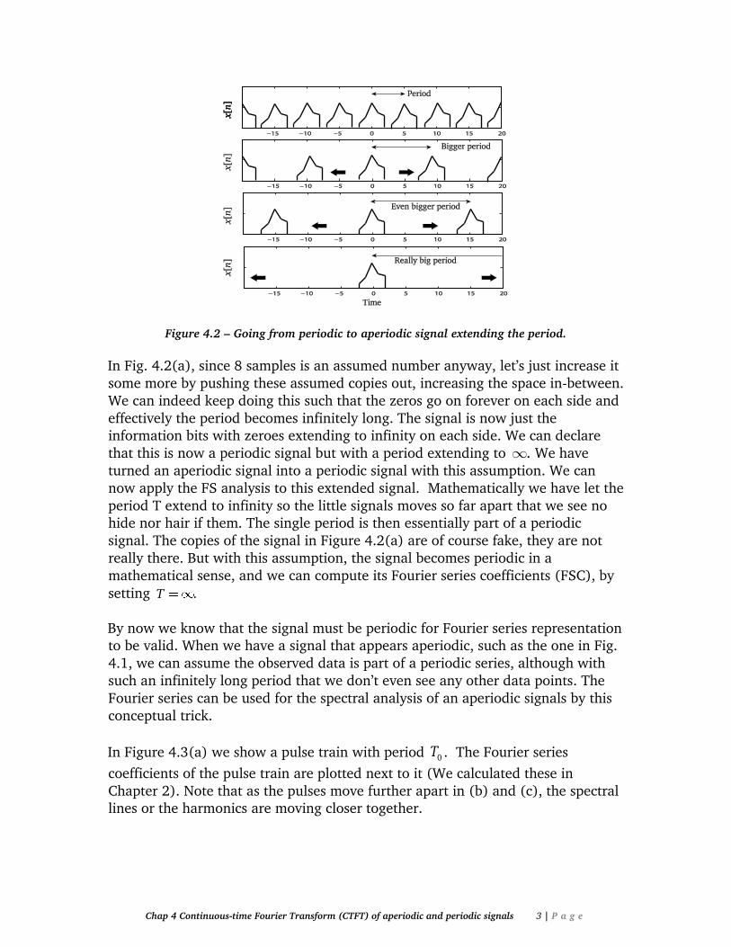
Figure 4.2 – Going from periodic to aperiodic signal extending the period.

In Fig. 4.2(a), since 8 samples is an assumed number anyway, let’s just increase it some more by pushing these assumed copies out, increasing the space in-between. We can indeed keep doing this such that the zeros go on forever on each side and effectively the period becomes infinitely long. The signal is now just the information bits with zeroes extending to infinity on each side. We can declare that this is now a periodic signal but with a period extending to We have turned an aperiodic signal into a periodic signal with this assumption. We can now apply the FS analysis to this extended signal. Mathematically we have let the period T extend to infinity so the little signals moves so far apart that we see no hide nor hair if them. The single period is then essentially part of a periodic signal. The copies of the signal in Figure 4.2(a) are of course fake, they are not really there. But with this assumption, the signal becomes periodic in a mathematical sense, and we can compute its Fourier series coefficients (FSC), by setting .T By now we know that the signal must be periodic for Fourier series representation to be valid. When we have a signal that appears aperiodic, such as the one in Fig. 4.1, we can assume the observed data is part of a periodic series, although with such an infinitely long period that we don’t even see any other data points. The Fourier series can be used for the spectral analysis of an aperiodic signals by this conceptual trick.

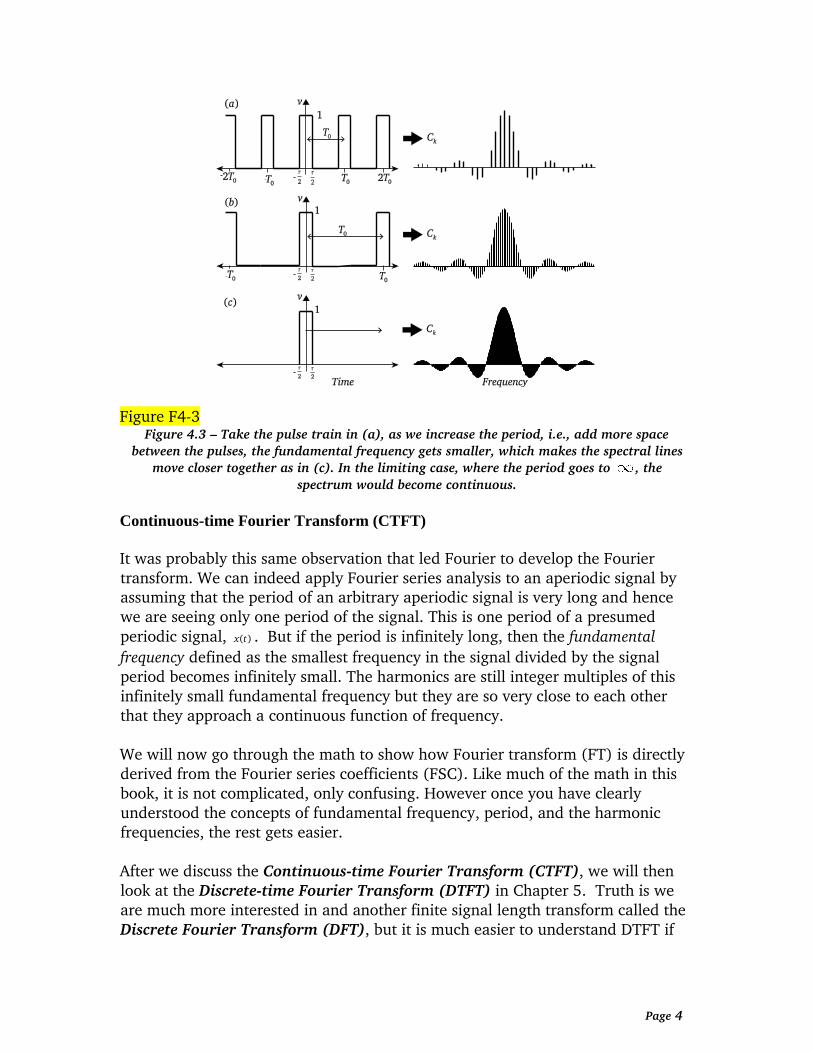
In Figure 4.3(a) we show a pulse train with period 0T . The Fourier series

coefficients of the pulse train are plotted next to it (We calculated these in Chapter 2). Note that as the pulses move further apart in (b) and (c), the spectral lines or the harmonics are moving closer together.

Figure F4-3 Figure 4.3 – Take the pulse train in (a), as we increase the period, i.e., add more space

between the pulses, the fundamental frequency gets smaller, which makes the spectral lines

move closer together as in (c). In the limiting case, where the period goes to , the

spectrum would become continuous.

Continuous-time Fourier Transform (CTFT)

It was probably this same observation that led Fourier to develop the Fourier transform. We can indeed apply Fourier series analysis to an aperiodic signal by assuming that the period of an arbitrary aperiodic signal is very long and hence we are seeing only one period of the signal. This is one period of a presumed periodic signal, ( )x t . But if the period is infinitely long, then the fundamental

frequency defined as the smallest frequency in the signal divided by the signal period becomes infinitely small. The harmonics are still integer multiples of this infinitely small fundamental frequency but they are so very close to each other that they approach a continuous function of frequency. We will now go through the math to show how Fourier transform (FT) is directly derived from the Fourier series coefficients (FSC). Like much of the math in this book, it is not complicated, only confusing. However once you have clearly understood the concepts of fundamental frequency, period, and the harmonic frequencies, the rest gets easier. After we discuss the Continuous-time Fourier Transform (CTFT), we will then look at the Discrete-time Fourier Transform (DTFT) in Chapter 5. Truth is we are much more interested in and another finite signal length transform called the Discrete Fourier Transform (DFT), but it is much easier to understand DTFT if


we start with the continuous-time case first. So although you will come across CTFT only in books and school, it is essential for the full understanding of this topic.

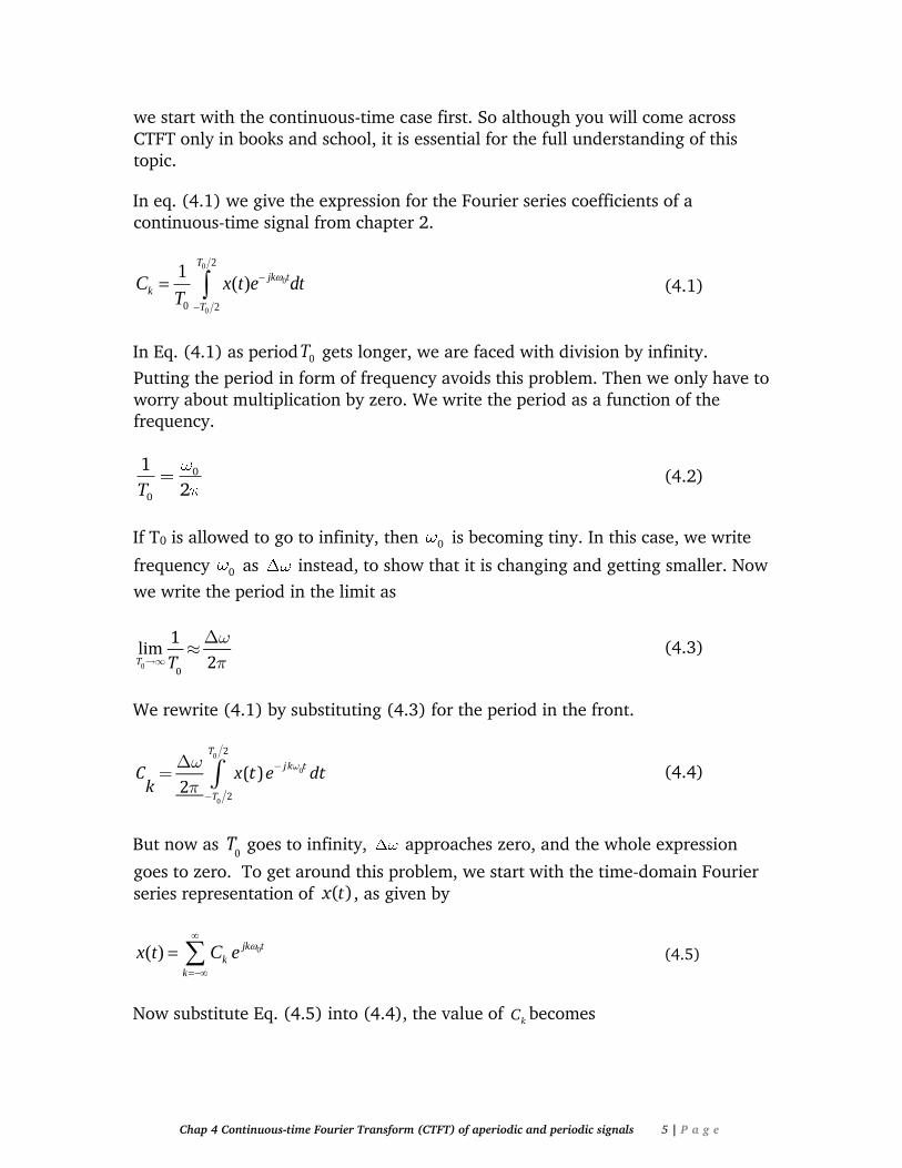
In eq. (4.1) we give the expression for the Fourier series coefficients of a continuous-time signal from chapter 2.

0

0

0

2

0 2

1( )

T

jk t

k

T

C x t e dtT

(4.1)

In Eq. (4.1) as period 0T gets longer, we are faced with division by infinity.

Putting the period in form of frequency avoids this problem. Then we only have to worry about multiplication by zero. We write the period as a function of the frequency.

0

0

1

2T (4.2)

If T0 is allowed to go to infinity, then 0 is becoming tiny. In this case, we write

frequency 0 as instead, to show that it is changing and getting smaller. Now

we write the period in the limit as

(4.3)

We rewrite (4.1) by substituting (4.3) for the period in the front.

(4.4)

But now asT

0 goes to infinity, approaches zero, and the whole expression

goes to zero. To get around this problem, we start with the time-domain Fourier series representation of ( )x t , as given by

0( )jk t

k

k

x t C e

(4.5)

Now substitute Eq. (4.5) into (4.4), the value of kC becomes

(4.6)

In this expression, the summation outside can be replaced by an integral because we are now multiplying the coefficients (the middle part) with dt , sort of like computing an infinitesimal area. We change to d , and 0k to , the

continuous frequency. We also move the factor 1 2 outside. Now we rewrite Eq.

(4.6) incorporating these ideas as

(4.7)

We give the underlined part a special name, calling it the Fourier transform and refer to it by ( )X . Substituting this nomenclature in (4.7) for the underlined

part, we write it in a new form. This expression is called the Inverse Fourier transform and is equivalent to the Fourier series representation or the synthesis equation.

(4.8)

The Continuous-time Fourier Transform (CTFT) is defined as the underlined part in (4.8). From Eq. (4.7) and is equal to

(4.9)

In referring to the Fourier transform, the following terminology is often used. If ( )x t is a time function, then its Fourier transform is written with a capital letter.

Such as for time-domain signal, ( )y t the CTFT would be written as ( )Y . These

two terms are called a transform pair and often written with a bidirectional arrow in between them such as here.


The symbol . is also used to denote the Fourier Transform. The symbol 1 . is used to denote the inverse transform such that

The CTFT is generally a complex function. We can plot the real and the imaginary parts of the transform, or we can compute and plot the magnitude, referred to as

( )X and the phase, referred to as ( )X . The magnitude is computed by taking

the square root of the product *( ) ( )X X and phase by the arctan of the ratio of the

imaginary and the real parts. We can also write the transform this way, separating out the magnitude and the phase spectrums.

( )( ) ( ) j XX X e

Here

Magnitude Spectrum: ( )

: ( )

X

Phase Spectrum X

In fact the magnitude is almost always given in dBs.

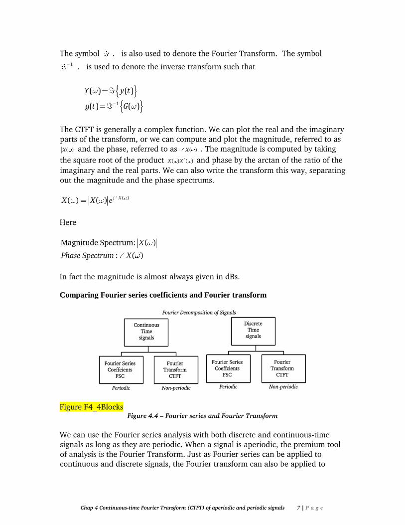
Comparing Fourier series coefficients and Fourier transform

Figure F4_4Blocks

Figure 4.4 – Fourier series and Fourier Transform

We can use the Fourier series analysis with both discrete and continuous-time signals as long as they are periodic. When a signal is aperiodic, the premium tool of analysis is the Fourier Transform. Just as Fourier series can be applied to continuous and discrete signals, the Fourier transform can also be applied to

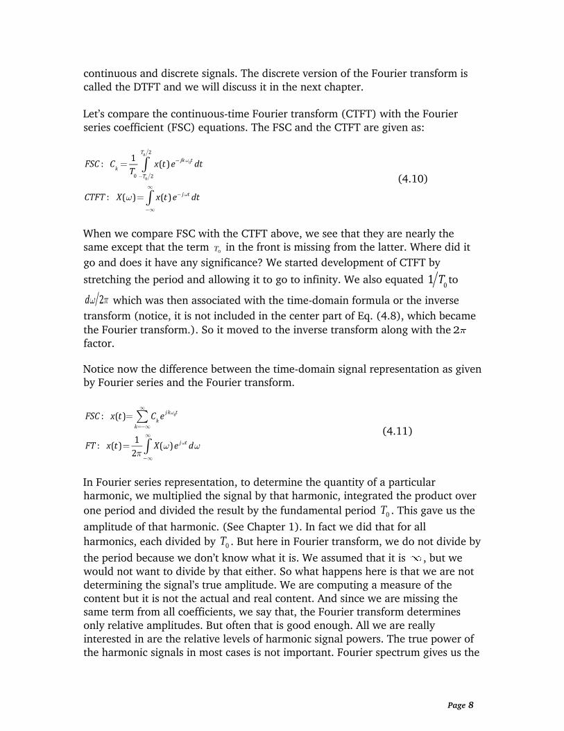
continuous and discrete signals. The discrete version of the Fourier transform is called the DTFT and we will discuss it in the next chapter. Let’s compare the continuous-time Fourier transform (CTFT) with the Fourier series coefficient (FSC) equations. The FSC and the CTFT are given as:

(4.10)

When we compare FSC with the CTFT above, we see that they are nearly the same except that the term

0T in the front is missing from the latter. Where did it

go and does it have any significance? We started development of CTFT by

stretching the period and allowing it to go to infinity. We also equated 1 T

0to

which was then associated with the time-domain formula or the inverse

transform (notice, it is not included in the center part of Eq. (4.8), which became

the Fourier transform.). So it moved to the inverse transform along with the 2

factor.

Notice now the difference between the time-domain signal representation as given by Fourier series and the Fourier transform.

(4.11)

In Fourier series representation, to determine the quantity of a particular harmonic, we multiplied the signal by that harmonic, integrated the product over

one period and divided the result by the fundamental period 0T . This gave us the

amplitude of that harmonic. (See Chapter 1). In fact we did that for all

harmonics, each divided by 0T . But here in Fourier transform, we do not divide by

the period because we don’t know what it is. We assumed that it is , but we would not want to divide by that either. So what happens here is that we are not determining the signal’s true amplitude. We are computing a measure of the content but it is not the actual and real content. And since we are missing the same term from all coefficients, we say that, the Fourier transform determines only relative amplitudes. But often that is good enough. All we are really interested in are the relative levels of harmonic signal powers. The true power of the harmonic signals in most cases is not important. Fourier spectrum gives us the


relative distribution of power among the various harmonic frequencies in the signal. In practice, we often normalize the maximum power to 0 dB such that the relative levels are consistent among all frequency components.

CTFT of aperiodic signals

Now we will take a look at some important aperiodic signals and their transforms. In the process, we will use the following important properties which can be used to compute the Fourier transform of many functions.

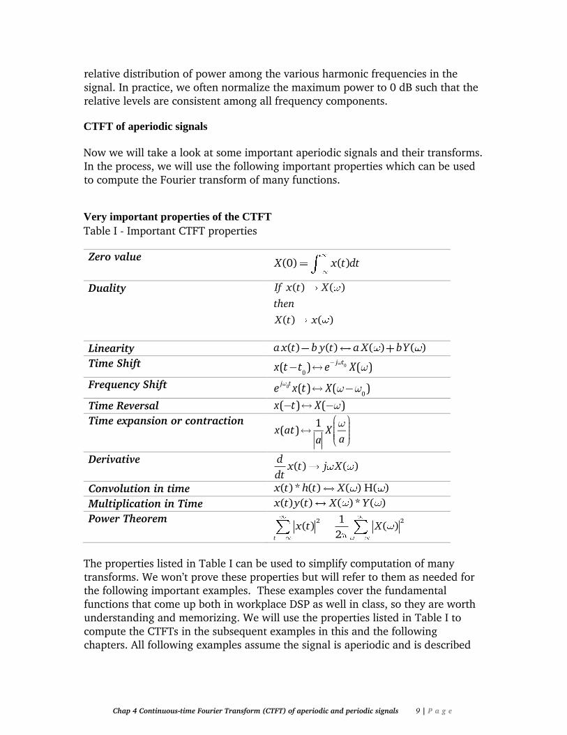
Very important properties of the CTFT

Table I - Important CTFT properties

Zero value (0) ( )X x t dt

Duality

( ) ( )

( ) ( )

If x t X

then

X t x

Linearity ( ) ( ) ( ) ( )a x t b y t a X bY

Time Shift

Frequency Shift

Time Reversal

Time expansion or contraction

Derivative ( ) ( )d

x t j Xdt

Convolution in time ( )* ( ) ( ) H( )x t h t X

Multiplication in Time ( ) ( ) ( )* ( )x t y t X Y

Power Theorem 2 21( ) ( )

2t

x t X

The properties listed in Table I can be used to simplify computation of many transforms. We won’t prove these properties but will refer to them as needed for the following important examples. These examples cover the fundamental functions that come up both in workplace DSP as well in class, so they are worth understanding and memorizing. We will use the properties listed in Table I to compute the CTFTs in the subsequent examples in this and the following chapters. All following examples assume the signal is aperiodic and is described

by continuous-time. The Fourier transform in these examples will be referred to as CTFT. CTFT of an impulse function

The delta function can be considered a continuous or a discrete function, but here we treat it as a continuous function. To compute its CTFT, we use the expression in Eq. (4.9) for the CTFT and substitute delta function for function ( ).x t

In the third step, we used the sifting property of the delta function. The sifting property sates that the integral of the product of a continuous-time signal by a delta function isolates the value of the signal at the location of the delta function.

( ) ( ) ( )t a x t dt x a

In this case since delta is un-shifted, or a = 0. The isolated value of the complex exponential is 1.0 at the origin. The integrand becomes a constant, so it is no longer a function of frequency. Hence CTFT is a constant for all frequencies. We get a flat line for the spectrum of the delta function. The delta function is defined as a summation of an infinite number of frequencies as we see in its definition in Eq. (4.12). In its transform, we see a spectrum that encompasses the whole of the frequency space to infinity, hence a flat line from

. The delta function is defined as

(4.12)

It is also given as


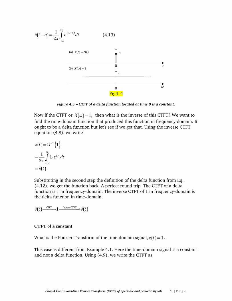
(4.13)

Fig4_4

Figure 4.5 – CTFT of a delta function located at time 0 is a constant.

Now if the CTFT or then what is the inverse of this CTFT? We want to

find the time-domain function that produced this function in frequency domain. It ought to be a delta function but let’s see if we get that. Using the inverse CTFT equation (4.8), we write

Substituting in the second step the definition of the delta function from Eq. (4.12), we get the function back. A perfect round trip. The CTFT of a delta function is 1 in frequency-domain. The inverse CTFT of 1 in frequency-domain is the delta function in time-domain.

CTFT of a constant

What is the Fourier Transform of the time-domain signal, .

This case is different from Example 4.1. Here the time-domain signal is a constant and not a delta function. Using (4.9), we write the CTFT as

Using Eq. (4.12) again the expression for the delta function, we get the CTFT of the constant 1 as

It can be a little confusing why there is this factor, but it is coming from the definition of the delta function.

Figure F4_6 Figure 4.6 – CTFT of a constant function which shows reciprocal relationship with example

4.1.

If the time-domain signal is a constant, then its Fourier Transform is the delta function and if we were to do the inverse transform of we would get back

( ) 1.x t We can write this pair as

Note in example 4.1, we had this pair

Which is confusingly similar but is not the same thing at all. CTFT of a sinusoid

Since a sinusoid is a periodic function, we will select only one period of it to make it aperiodic. Here we have just a piece of a sinusoid. We make no assumption about what happens outside the selected time frame. The cosine wave shown in


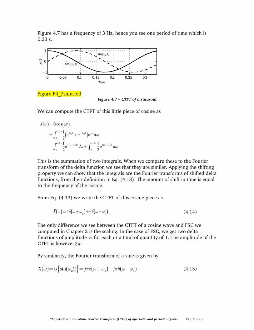
Figure 4.7 has a frequency of 3 Hz, hence you see one period of time which is 0.33 s.

Figure F4_7sinusoid

Figure 4.7 – CTFT of a sinusoid

We can compute the CTFT of this little piece of cosine as

This is the summation of two integrals. When we compare these to the Fourier transform of the delta function we see that they are similar. Applying the shifting property we can show that the integrals are the Fourier transforms of shifted delta functions, from their definition in Eq. (4.13). The amount of shift in time is equal to the frequency of the cosine. From Eq. (4.13) we write the CTFT of this cosine piece as

(4.14)

The only difference we see between the CTFT of a cosine wave and FSC we computed in Chapter 2 is the scaling. In the case of FSC, we get two delta functions of amplitude ½ for each or a total of quantity of 1. The amplitude of the CTFT is however . By similarity, the Fourier transform of a sine is given by

(4.15)

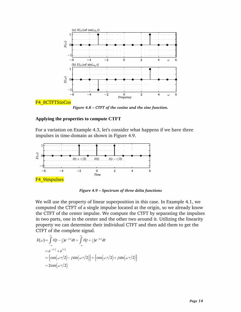
F4_8CTFTSinCos

Figure 4.8 – CTFT of the cosine and the sine function.

Applying the properties to compute CTFT

For a variation on Example 4.3, let’s consider what happens if we have three impulses in time-domain as shown in Figure 4.9.

F4_9impulses

Figure 4.9 – Spectrum of three delta functions

We will use the property of linear superposition in this case. In Example 4.1, we computed the CTFT of a single impulse located at the origin, so we already know the CTFT of the center impulse. We compute the CTFT by separating the impulses in two parts, one in the center and the other two around it. Utilizing the linearity property we can determine their individual CTFT and then add them to get the CTFT of the complete signal.


We know from Example 4.1 that the CTFT of an impulse at the origin is a constant. So the CTFT of this signal is

The CTFT of the three equal impulses is a sinusoid with mean value of 1.0.

CTFT of a complex exponential of frequency

Now we calculate the CTFT of the ubiquitous complex exponential given by

A CE is really two functions, one a cosine of frequency 0 and the other a sine of

the same frequency.

F4_10exp

Figure 4.10 – The CTFT of a complex exponential

We determined the CTFT of the sine and cosine in Example 4.4 given by

Now since

0

0 0( ) cos( ) sin( )j tx t e t j t

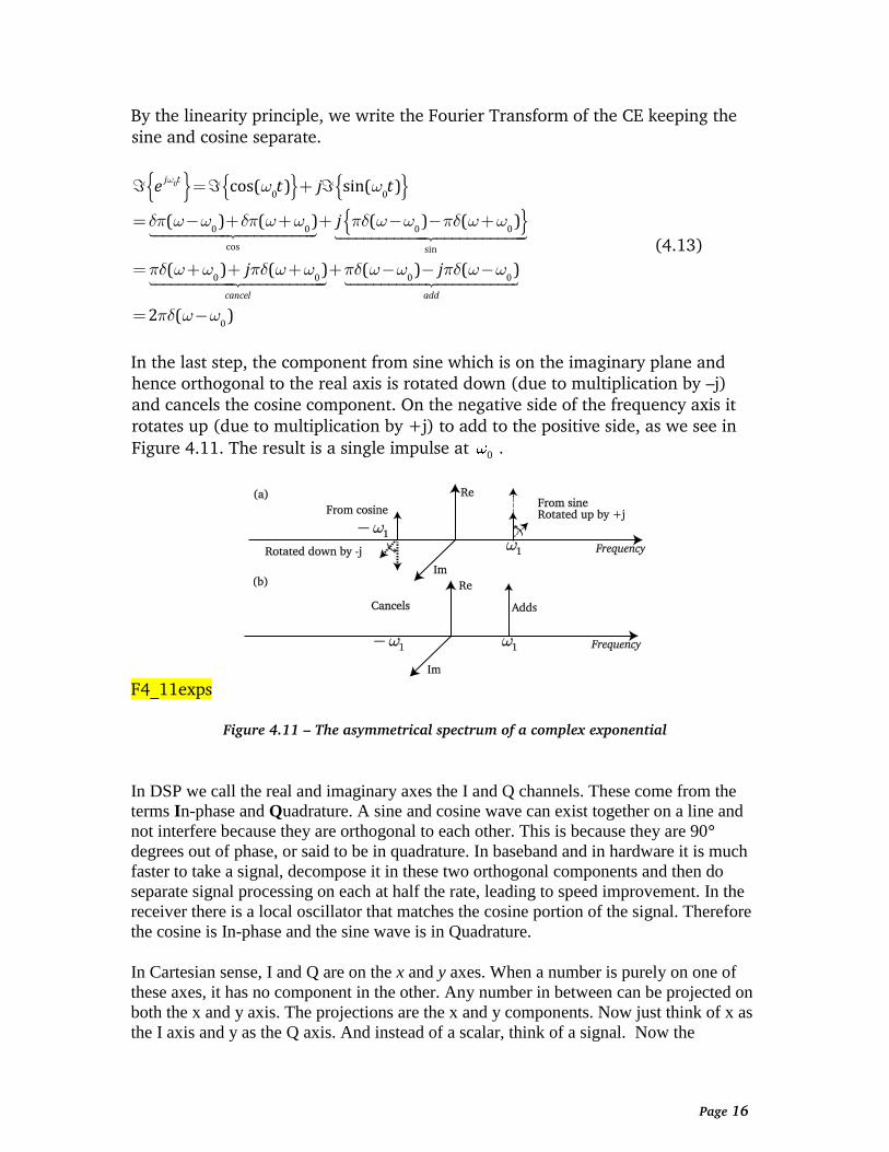
By the linearity principle, we write the Fourier Transform of the CE keeping the sine and cosine separate.

(4.13)

In the last step, the component from sine which is on the imaginary plane and hence orthogonal to the real axis is rotated down (due to multiplication by –j) and cancels the cosine component. On the negative side of the frequency axis it rotates up (due to multiplication by +j) to add to the positive side, as we see in

Figure 4.11. The result is a single impulse at 0 .

F4_11exps

Figure 4.11 – The asymmetrical spectrum of a complex exponential

In DSP we call the real and imaginary axes the I and Q channels. These come from the

terms In-phase and Quadrature. A sine and cosine wave can exist together on a line and

not interfere because they are orthogonal to each other. This is because they are 90°

degrees out of phase, or said to be in quadrature. In baseband and in hardware it is much

faster to take a signal, decompose it in these two orthogonal components and then do

separate signal processing on each at half the rate, leading to speed improvement. In the

receiver there is a local oscillator that matches the cosine portion of the signal. Therefore

the cosine is In-phase and the sine wave is in Quadrature.

In Cartesian sense, I and Q are on the x and y axes. When a number is purely on one of

these axes, it has no component in the other. Any number in between can be projected on

both the x and y axis. The projections are the x and y components. Now just think of x as

the I axis and y as the Q axis. And instead of a scalar, think of a signal. Now the


projections are the “amount” of cosine on the I axis and “amount” of sine on the Q axis. I

axis represents the cosine projection and Q axis the sine projection of a signal. When

multiplying by j, the phase changes by 90°. This is the same as moving from one axis to

the other axis.

Now consider an Inverse-CTFT (also referred to as taking the iCTFT) that consists

of a single impulse located at frequency 1 written as

We want to know what time-domain function produced this spectrum. We take the iCTFT.

1

11

1

( )

1( )

2

1

2

j t

j t

x t

e d

e

The result is a complex exponential of frequency 1 in the time-domain. Because

this is a complex signal, it has a non-symmetrical frequency response which consists of just one impulse located at the CE’s frequency. In Fig. 4.11, we see why it is one sided. The reason is that a cancellation occurs on the negative side and an addition on the positive side of the frequency axis. The component from the sine rotates up to add to cosine part on the positive and rotates down on the negative side to cancel the cosine portion. This of course is coming from the Euler’s equation. Here we write the two important CTFT pairs. The CTFT of a CE is one-sided, an impulse at its frequency.

Time-shifting a function

What is the CTFT of a delta function shifted by time 0t ? This is a very important

case because we can construct many signals as summation of time-shifted delta functions. This case is very important to further understanding of discrete signals. We can determine the response of a delayed signal by noting the time shift property in Table I. The property says that if a function is delayed by a time

period of 0

t , then in frequency domain, the original response of the un-delayed

signal is multiplied by a CE of frequency 0j te . This is given by the product of 0( ) and j tX e , where ( )X is the Fourier Transform of the un-delayed signal.

Look carefully at this signal, 0j te . Note that time is constant and hence this is a frequency-domain signal, with frequency as the variable.

We write the shifted signal as . Calculate the Fourier Transform of

this function from Eq. (4.9) as

In row 3, we set 0t t which makes the integrand a constant. What we get in

frequency domain for this delayed delta function is a CE. This CE has the form 0j te and is confusing. That’s because we are not used to seeing exponentials in

the frequency domain, but there is of course no law against it. Now intuitively speaking, if you have a signal and you move it from one “place” to another, does anything change about the signal? Similarly, delaying a signal does not change its amplitude (the main parameter by which we characterize signals.). Its frequency also does not change, but what does change is its phase. If a sine wave is running

and we arrive to look at it at time 0t after it has started, we are going to see an

instantaneous phase at that time which will be different depending on when we arrive on the scene. That’s all a time shift does. We can show this by computing the magnitude and the phase of the spectrum of the delayed signal. We first compute the magnitude of the delayed signal. Here we write that the magnitude of the delayed signal as the magnitude of the

product of the original spectrum and the CE 0j te .

We compute the magnitude of the CE first. Keep in mind that this is not a time-domain signal. The variable is frequency, and not time. The CE is given in the Euler form as


We compute the magnitude of this signal by

0

0 0

2 20 0

cos( ) sin( )

cos ( ) sin ( )

1

j te t j t

t t

Being a sinusoid, even if a complex one in frequency-domain, its magnitude is still 1.0 from a simple trigonometric relationship. Then we compute the magnitude of the shifted function, which is the product of the un-delayed signal magnitude and the magnitude of the CE.

0

0

*

(

( )

( ) 1

( ) ( )

( )

j t

Mag x t t

X e

X

X X

X

So here we see that the magnitude of the delayed signal is same as that of the un-delayed signal. Delay does not change the magnitude. From the same equation, we see that the magnitude is a function of the same frequency variable and has not been modified by the process. So what did change by shifting the signal in time? Now we look at the phase. The phase delay was

The phase response of the delayed signal is given by

Since this is a function of the delay, the phase has indeed changed from the un-delayed case. The conclusion we draw is that delaying a signal changes its phase response, or equivalently multiplication by a CE in the frequency domain changes the phase of a signal. This property is used in simulation to add phase shifts to a signal.

In general, if we shift a signal by time 0t , the Fourier transform of the signal can

be calculated by the time shift property as

0

0( ) ( )j tx t t e X (4.17)

F4_12timeshift Figure 4.12 – Signal delay causes only the phase response to change. In (a) we see an arbitrary

signal delayed by 2 seconds and in (b), it has been delayed 4 seconds in €. Both cases keep the

same magnitude but their phases are different.

In Figure 4.12 we show the effect of time-delay. In (a), we have a signal with an arbitrary spectrum centered at frequency of 2 Hz. We don’t actually show this signal, only its Fourier Transform, with x-axis being frequency. You only need to note its shape and center location on the frequency axis. Now we delay this signal by 2 seconds (we don’t know what the signal is, but that does not matter.) and want to see what happened to the spectrum.

In (b) we draw the CE 0j te with 0 2.t (both sine and cosine are shown In (c),

we see the effect of multiplying this CE by the spectrum in (a). The magnitude is unchanged. But when we look at (d) we see the phase. Since we do not know what the previous phase was no statement can be made, yet.


Now we examine the second column. In this case the signal is delayed by 4 seconds. Once again in (g) we see no change in magnitude but we see that phase in (h) has indeed changed from pervious case in (d). Duality with frequency shift

If a signal is shifted in time, the response changes for phase but not for frequency.

Now what if we shift the spectrum by frequency such as ( )X vs. 0( )X . The

response is to be shifted by a constant frequency shift of 0. We can do this by

using the frequency shift property. The CTFT of the frequency-shifted signal changes as

(4.18)

If we multiply a time-domain signal by a CE of a desired frequency, the result is a shifted frequency response by the new frequency.

(4.19)

Neither the frequency nor the time shifts change the magnitude of the spectrum. The only thing that changes is the phase. The frequency shift property is also called the modulation property. We think of modulation as multiplying a signal by a carrier and in-fact if you look at Eq. (4.18), that is exactly what we are doing. The CE can be thought of as a carrier signal, a complex sinusoid of a single carrier

frequency. A time-domain signal multiplied by a CE, 0j te results in the signal transferring to the carrier frequency without change in its amplitude. Time scaling

Here we look at what happens to a spectrum if a signal is compressed or

expanded in time-domain. If the unscaled signal has a spectrum ,

then the spectrum of the scaled signal is given by

(4.20)

Where a is the scale factor. This can be greater than 1 for expansion or less than 1 for compression. As we see in Fig. 4.13, if a signal is spread in time by a factor a , then in frequency domain the spectrum contracts by the same factor.

Figure 4.13 – Effect of time scaling

F4_13timeexpansion CTFT of a step function

Find the CTFT of a unit step function, ( ) ( )x t u t .

Figure 4.14 – CTFT of a unit step function

F4_14unitstep There are a couple of different approaches we can use to compute the CTFT of the unit step function. Here we use the derivative property and the linearity property. First, we find two continuous functions, the CTFT of which we know. The two


functions are a constant of amplitude one-half and a signum function of the same amplitude. When these are summed, we get the one-sided step function, ( ).u t

The derivative of the signum function is the delta function. So we have

From the derivative property, we write

1 1 1 1( ) 2 ( )

2 2

1( )

u tj j

j The magnitude of the function is a constant and the phase is linear.

Convolution property

The most important result from Fourier Transform is the convolution property. In fact Fourier transform is often used to perform convolution in hardware instead of doing convolution in time-domain. The property is given by

(4.21)

In time-domain, convolution is a resource-heavy computation. Calculating integrals is more costly in terms of time than simple multiplication. But convolution can be done using the Fourier transform convolution property. The convolution property states:

(4.22)

This says that the convolution of two signals can be computed by multiplying their individual Fourier transforms and then taking the inverse transform of the product. In many cases this is simpler to do. We can prove this as follows. We will write the time-domain expression for the convolution and then take its Fourier transform. Yes, it does look messy and requires fancy calculus.

Now we interchange the order of integration to get this from.

Now we make a variable change by setting . Using this, we get

This can be written as

Now we move the term out of the inner integral because it is not function of

u to get the desired result and complete the convolution property proof.

The duality property of Fourier transform then implies that if we multiply two signals in time-domain, then the Fourier transform of their product would be equal to convolution of the two transforms.


(4.23)

This is an efficient way to compute convolution. Convolution can be hard to visualize. The one way to think of it is as smearing or a smoothing process. The convolution process produces the smoothed version of one of the signals as we can see in Figure 4.15.

Figure 4.15 - (a) ( )x t (b) ( )y t and (c) is the convolution of the two signals using Fourier

transform. In each case the result is smoother than either of the original signals.

F4_15convoa CTFT of a causal signal

Making things a little complicated, we are given a causal signal.

( ) ( )atx t e u t

Figure 4.16 – The one-sided exponential function

F4_16onesided From the definition of CTFT, we write

This integral is equal to

We can compute the magnitude of this signal as

2 2

1 1( )X

a j a

And the phase is computed as

Figure 4.17 – The magnitude and phase of the CTFT of the one-sided exponential function

F4_17CTFTconvo CTFT of a one-sided exponential

We want to find the CTFT of the function 0( ) ( )cos( )atx t e u t t .

We can write this as the product of these two signals.


Where first signal is as in Example 4.7 and the second is a cosine wave. By the convolution property, we write

We know the CTFT of both of these functions from Example 4.7 and 4.3.

The convolution of these two functions is actually trivial and is given by

We plot the magnitude and see that the cosine CTFT impulses have managed to shift the response of the one-sided exponential on to the cosine frequency. We see two copies of the spectrum from Figure 4.17 but duplicated at each frequency. The same thing happens to the phase.

Figure 4.18 – The CTFT of the product of two signals.

F4_18CTFTconvo2 The convolution in this case was easy because the CTFT of the cosine are two delta functions. The convolution of a delta function with any function just transfers the function to the location of the delta function, so what we get is the

CTFT of the one-sided exponential at two frequencies, . So we see that the

convolution property can come in quite handy. Doing convolution using the FFT algorithm is more efficient than doing it in time domain. CTFT of a Gaussian function

Now we examine the CTFT of really unique and useful function, the Gaussian. The zero-mean Gaussian function is given by

2 221

( )2

tx t e

where is the signal variance. The CTFT of this function is very similar to the function itself.

2 2

2 2

2

2

1( )

2

1

2

t j t

t j t

X e e dt

e e dt

This is a difficult integral to solve but fortunately smart people have already done it for us. The result is

2 2

2 2

2

2

1( )

2

1

2

t j tX e e dt

e

Since is a constant, the shape of this curve is a function of the square of the frequency, same as it is in time-domain where it is square of time. Hence it is often said that the DTFT of the Gaussian function is same as itself, but what they really mean is that the shape is the same. This property of the Gaussian function is very important in nearly all fields. CTFT of the square pulse

Now we examine the CTFT of a square pulse of amplitude 1, with a period of , centered at time zero. This case is different from the one in Chapter 2 and Chapter 3 in that here we have just a single solitary pulse. This is not a case of repeating square pulses since in this section we are considering only aperiodic signals.


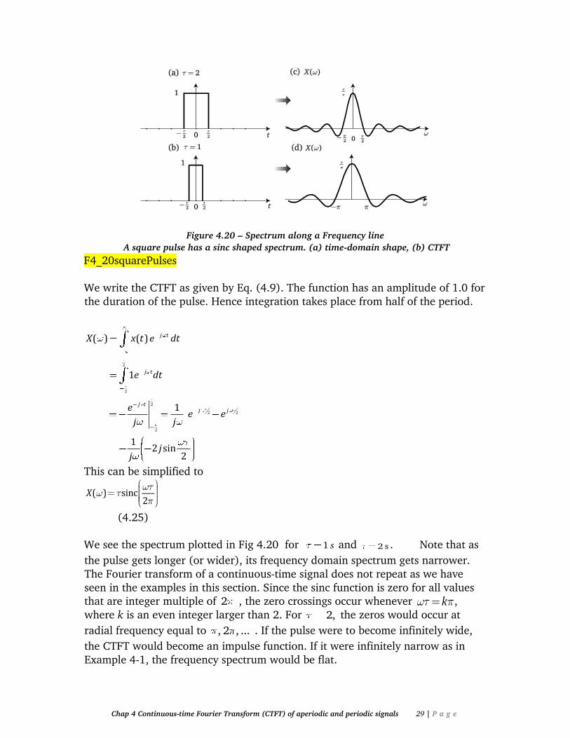
Figure 4.20 – Spectrum along a Frequency line

A square pulse has a sinc shaped spectrum. (a) time-domain shape, (b) CTFT

F4_20squarePulses We write the CTFT as given by Eq. (4.9). The function has an amplitude of 1.0 for the duration of the pulse. Hence integration takes place from half of the period.

2

2

2

2 2

2

( ) ( )

1

1

12 sin

2

j t

j t

j tj j

X x t e dt

e dt

ee e

j j

jj

This can be simplified to

(4.25) We see the spectrum plotted in Fig 4.20 for 1 s and 2 s . Note that as

the pulse gets longer (or wider), its frequency domain spectrum gets narrower. The Fourier transform of a continuous-time signal does not repeat as we have seen in the examples in this section. Since the sinc function is zero for all values that are integer multiple of 2 , the zero crossings occur whenever , where k is an even integer larger than 2. For 2, the zeros would occur at

radial frequency equal to , 2 , ... . If the pulse were to become infinitely wide,

the CTFT would become an impulse function. If it were infinitely narrow as in Example 4-1, the frequency spectrum would be flat.

Now assume that instead of the time-domain square pulse shown in Fig. 4.20, we are given a frequency response that looks like a square pulse. The spectrum is flat from -W to +W Hz. This can be imagined as the frequency response of an ideal

filter. Notice, that in the time-pulse case, we defined the half width of the pulse as

/ 2 , but here we define the half bandwidth by W and not by W/2. The reason is

that in time-domain, when a pulse is moved, its period is still . But bandwidth is designated as a positive quantity only. There is no such thing as a negative bandwidth. In this case, the bandwidth of the signal (because it is centered at 0 is said to be W Hz and not 2W Hz. However if this signal were moved to a higher frequency such that the whole signal was in the positive frequency range, it would be said to have a bandwidth of 2W Hz. This crazy definition gives rise to the concepts of low-pass and band-pass bandwidths. Lowpass is centered at the origin so it has half the bandwidth of bandpass. What time-domain signal produces a rectangular frequency response shown in Figure 4.21? The frequency response is limited to a certain bandwidth.

We compute the time-domain signal by the inverse CTFT equation.

Which can be simplified to

( ) sincW Wt

x t

Again we get a sinc function, but now in time-domain. This is the duality principle at work. This is a very interesting case and of fundamental importance in communications. A time-domain sinc shape has a very sharply defined shape in the frequency-domain. But a sinc function looks strange for a time-domain signal because it is not limited to a certain time period. But because it is “well-behaved”,


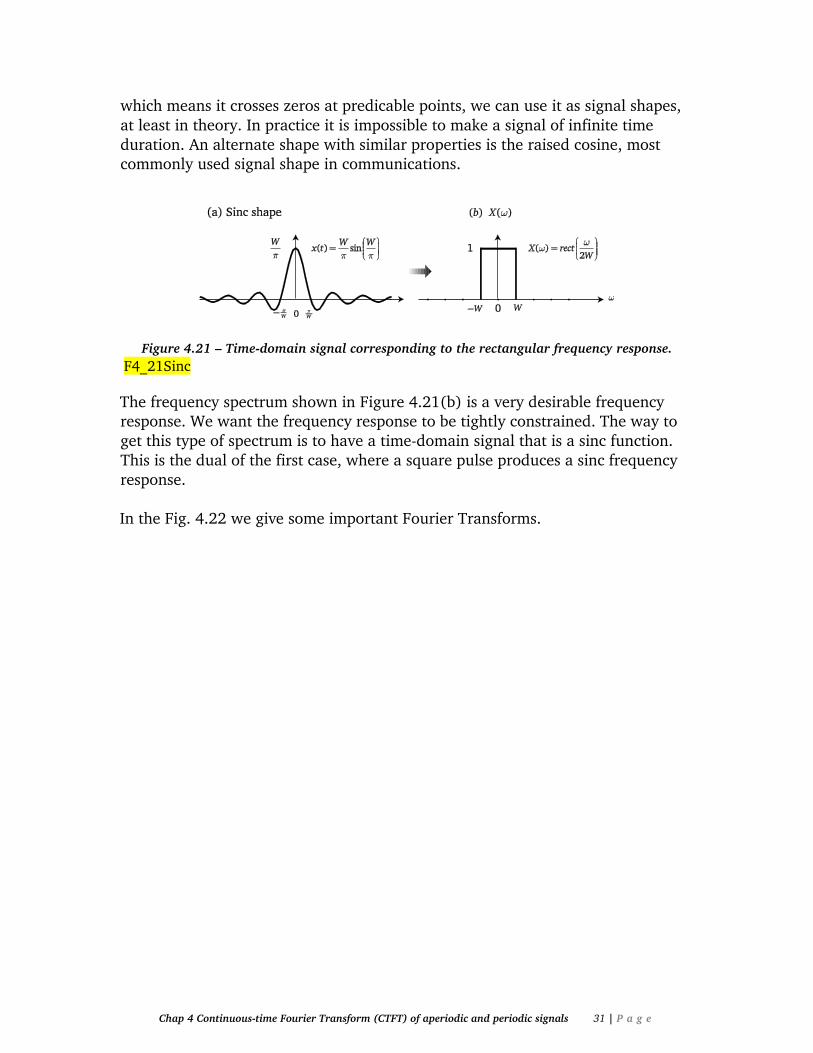
which means it crosses zeros at predicable points, we can use it as signal shapes, at least in theory. In practice it is impossible to make a signal of infinite time duration. An alternate shape with similar properties is the raised cosine, most commonly used signal shape in communications.

Figure 4.21 – Time-domain signal corresponding to the rectangular frequency response.

F4_21Sinc

The frequency spectrum shown in Figure 4.21(b) is a very desirable frequency response. We want the frequency response to be tightly constrained. The way to get this type of spectrum is to have a time-domain signal that is a sinc function. This is the dual of the first case, where a square pulse produces a sinc frequency response. In the Fig. 4.22 we give some important Fourier Transforms.

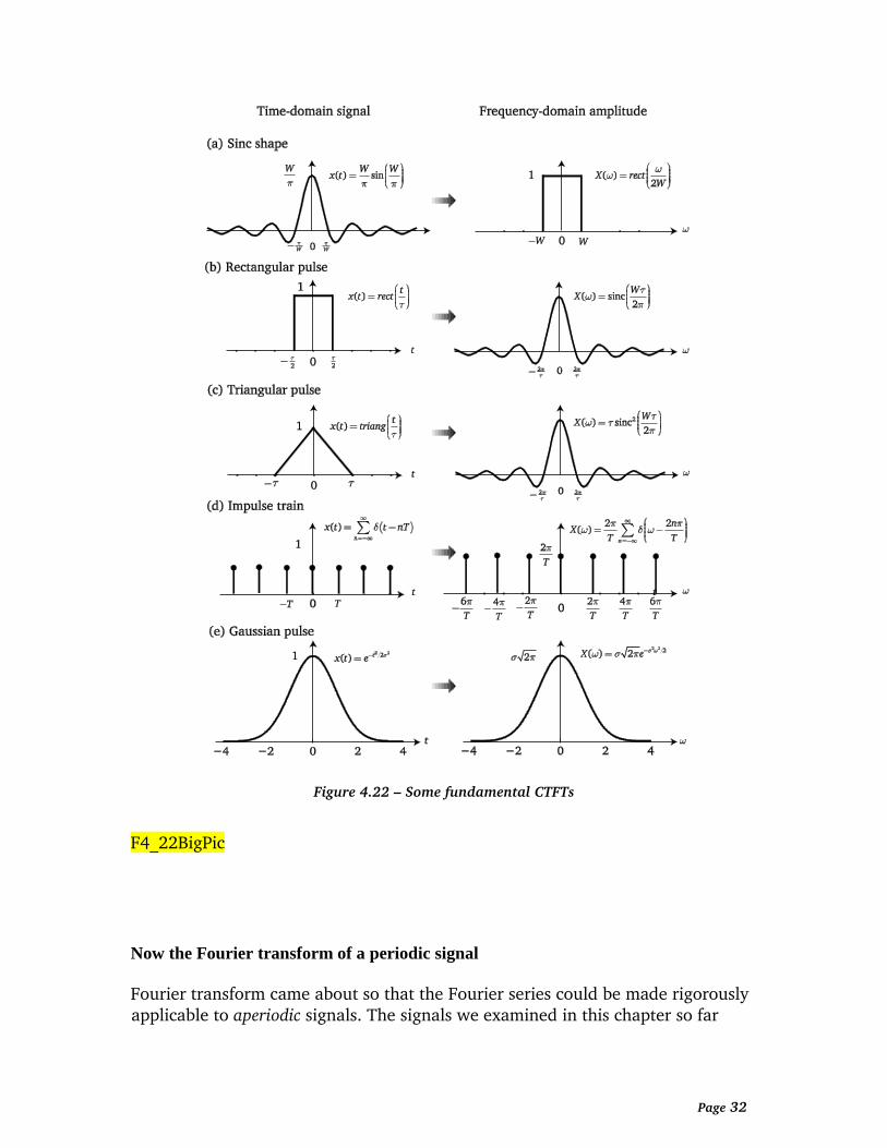
Figure 4.22 – Some fundamental CTFTs

F4_22BigPic

Now the Fourier transform of a periodic signal

Fourier transform came about so that the Fourier series could be made rigorously applicable to aperiodic signals. The signals we examined in this chapter so far


were all aperiodic, even the cosine wave, which we limited to one period. Can we use CTFT for a periodic signal? Our intuition says that this should be the same as the Fourier series. Let’s see if that is the case.

Take a periodic signal ( )x t with fundamental frequency of 0 02 T and write

its FS representation.

0( ) jk t

kk

x t C e

Taking the CTFT of both sides of this equation, we get

We can move the coefficients out because they are not function of frequency. They are just numbers.

The Fourier transform of a complex exponential 0j te is a delta function located at

the frequency 0. as we saw in Example 4.4. Making the substitution, we get

(4.26)

The delta function in (4.26) combs/sifts the coefficients and then repeats them

with fundamental frequency 0 . What does this equation say? It says that the

CTFT of a periodic signal, as opposed to the aperiodic signal, is a sampled version of the Fourier series coefficient of the aperiodic case. The best way to compute the CTFT of a periodic signal is to compute the Fourier series coefficients first and

then sample the coefficients at frequencies 0.k This results in a discrete

spectrum. The Fourier Transform of a periodic signal is a discrete form of the Fourier series coefficients that repeat with the frequency of the signal. Okay, this is admittedly strange. The CTFT of an aperiodic signal is continuous but the CTFT of a periodic signal is discrete? This is because a periodic signal has a finite period, hence the fundamental frequency is also a finite number which means that resolution is now a finite number hence the spectrum is discrete.

The CTFT of an aperiodic signal is aperiodic with continuous frequency. The CTFT of a periodic signal is periodic with its fundamental frequency and is discrete. It is also repeats the coefficients. All the CTFT properties we listed for aperiodic signals in Table I also apply to CTFT of periodic signals with one main consideration. The CTFT of periodic signal repeats. CTFT of a periodic impulse train

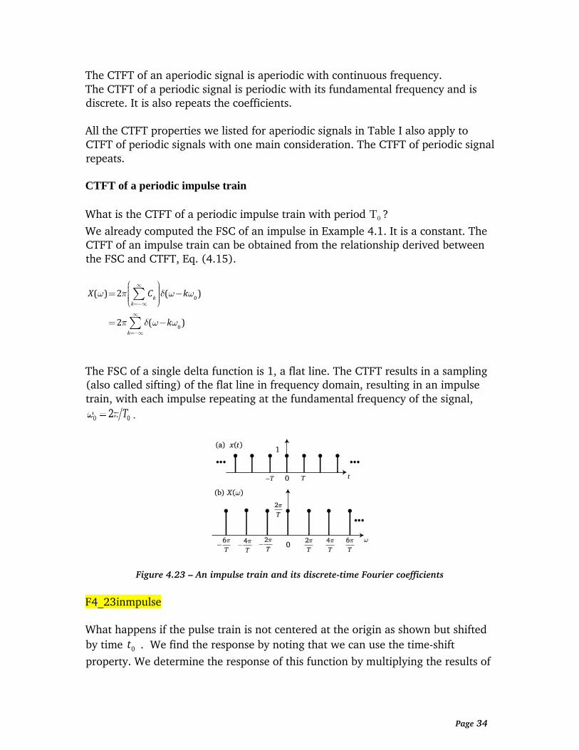
What is the CTFT of a periodic impulse train with period T0 ?

We already computed the FSC of an impulse in Example 4.1. It is a constant. The CTFT of an impulse train can be obtained from the relationship derived between the FSC and CTFT, Eq. (4.15).

The FSC of a single delta function is 1, a flat line. The CTFT results in a sampling (also called sifting) of the flat line in frequency domain, resulting in an impulse train, with each impulse repeating at the fundamental frequency of the signal,

0 02 T .

Figure 4.23 – An impulse train and its discrete-time Fourier coefficients

F4_23inmpulse What happens if the pulse train is not centered at the origin as shown but shifted

by time 0t . We find the response by noting that we can use the time-shift

property. We determine the response of this function by multiplying the results of


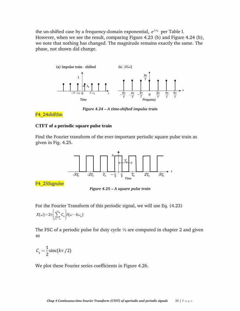
the un-shifted case by a frequency-domain exponential, 0j te per Table I. However, when we see the result, comparing Figure 4.23 (b) and Figure 4.24 (b), we note that nothing has changed. The magnitude remains exactly the same. The phase, not shown did change.

Figure 4.24 – A time-shifted impulse train

F4_24shiftIm CTFT of a periodic square pulse train

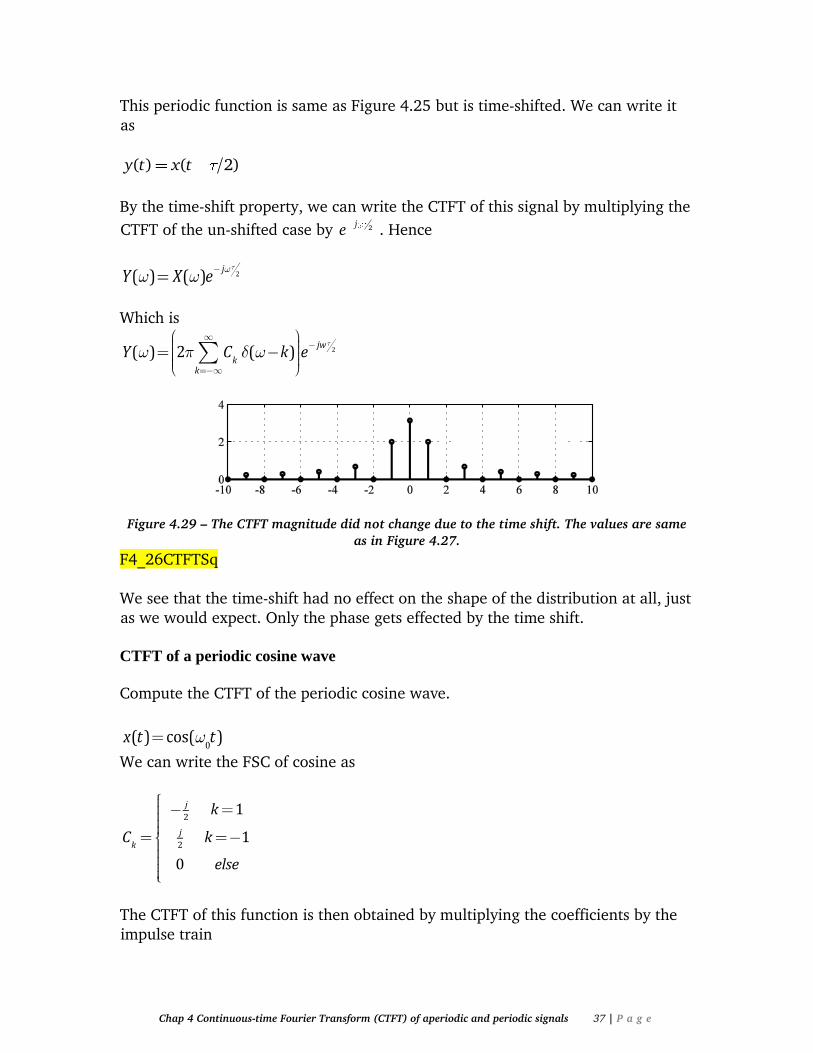
Find the Fourier transform of the ever-important periodic square pulse train as given in Fig. 4.25.

F4_25Sqpulse

Figure 4.25 – A square pulse train

For the Fourier Transform of this periodic signal, we will use Eq. (4.23)

The FSC of a periodic pulse for duty cycle ½ are computed in chapter 2 and given as

We plot these Fourier series coefficients in Figure 4.26.

Figure 4.26 – The Fourier series coefficients of a periodic square wave with duty cycle of .5.

F4_26FSC

To compute CTFT, we set 0 1 and now we write the CTFT expression as

Note that the CTFT is exactly the same as the FSC except the scale is larger than the FSC by a factor of by2 .

Figure 4.27 - The CTFT of the periodic square wave with a duty cycle of 0.5

F4_26CTFTSq The result is essentially the sampled version of the Fourier series coefficients scaled by 2 (see last example, Chapter 2) which are of course themselves

discrete. What if the square pulse was not centered at 0 but shifted some amount. We can compute the CTFT of this periodic function by applying the time shift property to the CTFT of the un-shifted square wave.

Figure 4.28 - A time-shifted square pulse train

F4_28Sqshifted


This periodic function is same as Figure 4.25 but is time-shifted. We can write it as

( ) ( 2)y t x t

By the time-shift property, we can write the CTFT of this signal by multiplying the

CTFT of the un-shifted case by 2je . Hence

Which is

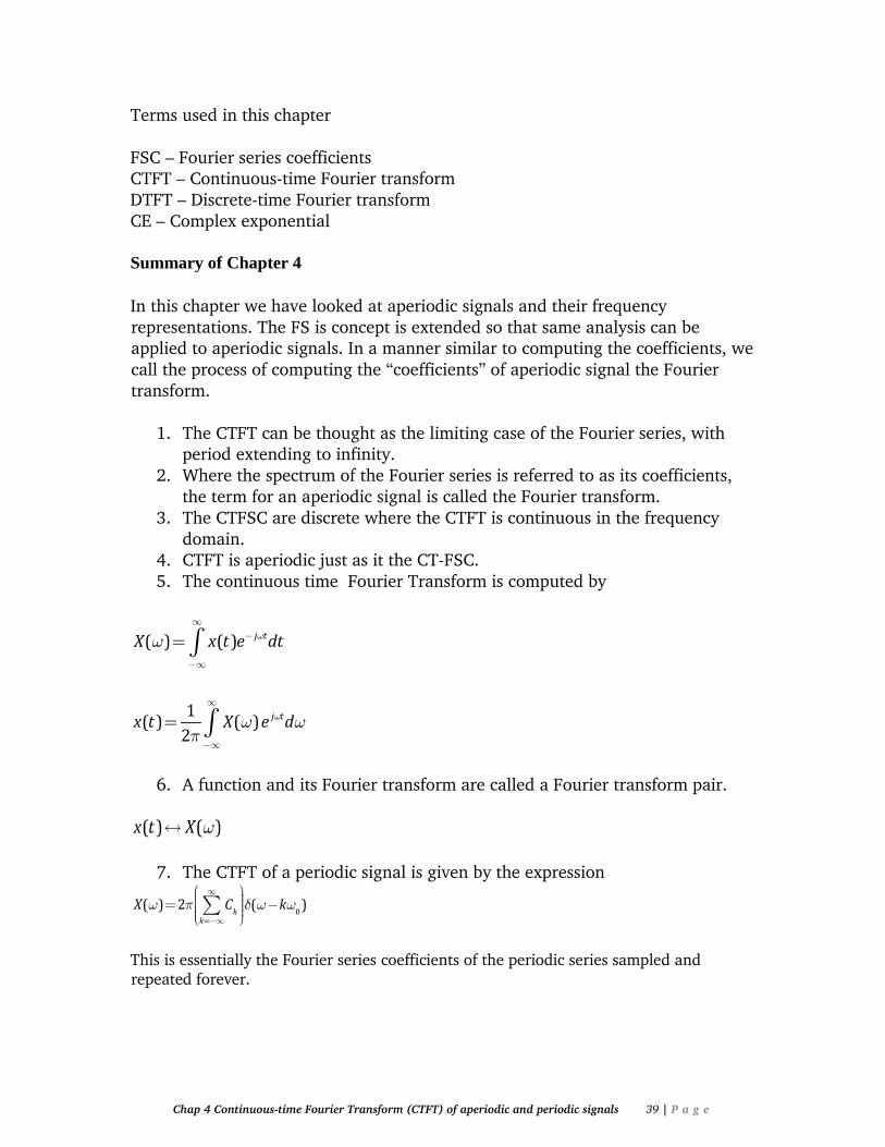
Figure 4.29 – The CTFT magnitude did not change due to the time shift. The values are same

as in Figure 4.27.

F4_26CTFTSq We see that the time-shift had no effect on the shape of the distribution at all, just as we would expect. Only the phase gets effected by the time shift. CTFT of a periodic cosine wave

Compute the CTFT of the periodic cosine wave.

We can write the FSC of cosine as

The CTFT of this function is then obtained by multiplying the coefficients by the impulse train

What we see directly is that in FSC the amplitude of each component was ½, and here it . The CTFT magnitude is 2 larger than the FSC. But other than that the result is exactly the same.


Terms used in this chapter FSC – Fourier series coefficients CTFT – Continuous-time Fourier transform DTFT – Discrete-time Fourier transform CE – Complex exponential Summary of Chapter 4

In this chapter we have looked at aperiodic signals and their frequency representations. The FS is concept is extended so that same analysis can be applied to aperiodic signals. In a manner similar to computing the coefficients, we call the process of computing the “coefficients” of aperiodic signal the Fourier transform.

1. The CTFT can be thought as the limiting case of the Fourier series, with period extending to infinity.

2. Where the spectrum of the Fourier series is referred to as its coefficients, the term for an aperiodic signal is called the Fourier transform.

3. The CTFSC are discrete where the CTFT is continuous in the frequency domain.

4. CTFT is aperiodic just as it the CT-FSC. 5. The continuous time Fourier Transform is computed by

6. A function and its Fourier transform are called a Fourier transform pair.

7. The CTFT of a periodic signal is given by the expression

This is essentially the Fourier series coefficients of the periodic series sampled and repeated forever.

8. The CTFT values are a factor 2 greater than the Fourier series coefficients calculated for the same signal.

9. The Fourier transform of a periodic signal is a repeated from the Fourier series coefficients for the same signal.

10. Unlike the CTFT of aperiodic signals, the CTFT of periodic signal is discrete.

Copyright 2015 Charan Langton All Rights reserved

Continuous-time Fourier Transform (CTFT) of aperiodic and...

Documents

Transcript of Continuous-time Fourier Transform (CTFT) of aperiodic and...