FOURIER EXPANSION OF EISENSTEIN SERIES ON … · FOURIER EXPANSION OF EISENSTEIN SERIES 4849 Using...
23
TRANSACTIONS OF THE AMERICAN MATHEMATICAL SOCIETY Volume 354, Number 12, Pages 4847–4869 S 0002-9947(02)03109-4 Article electronically published on August 1, 2002 FOURIER EXPANSION OF EISENSTEIN SERIES ON THE HILBERT MODULAR GROUP AND HILBERT CLASS FIELDS CLAUS MAZANTI SORENSEN Abstract. In this paper we consider the Eisenstein series for the Hilbert mod- ular group of a general number field. We compute the Fourier expansion at each cusp explicitly. The Fourier coefficients are given in terms of completed partial Hecke L-series, and from their functional equations, we get the func- tional equation for the Eisenstein vector. That is, we identify the scattering matrix. When we compute the determinant of the scattering matrix in the principal case, the Dedekind ξ-function of the Hilbert class field shows up. A proof in the imaginary quadratic case was given in Efrat and Sarnak, and for totally real fields with class number one a proof was given in Efrat. 1. Introduction Let us consider the group G = SL(2, R). It acts transitively on the upper half- plane X = H 2 = {z = x + iy ∈ C : y> 0} by linear fractional transformations. Thus for a g ∈ G and a z ∈ X , we have gz = az + b cz + d where g = a b c d ∈ G. The stabilizer at the point z = i is SO(2), and hence there is a homeomorphism H 2 ≈ SL(2, R)/ SO(2). We equip H 2 with the Poincar´ e metric, so as to get a Riemannian manifold: ds(z ) 2 = dx 2 + dy 2 y 2 . Then G acts by isometries. The associated G-invariant measure on H 2 is given by dμ(z )= dxdy y 2 . The theory of automorphic forms emerged from the study of functions on H 2 that are invariant/automorphic under some discrete subgroup of G = SL(2, R). The first such that comes to mind is the full elliptic modular group Γ = SL(2, Z)= γ = a b c d : a, b, c, d ∈ Z and ad - bc =1 . Received by the editors March 26, 2002 and, in revised form, May 13, 2002. 2000 Mathematics Subject Classification. Primary 11F30, 11F41, 11M36, 11R37, 11R42. Key words and phrases. Eisenstein series, Hilbert modular groups, Hilbert class fields. c 2002 American Mathematical Society 4847 License or copyright restrictions may apply to redistribution; see http://www.ams.org/journal-terms-of-use
Transcript of FOURIER EXPANSION OF EISENSTEIN SERIES ON … · FOURIER EXPANSION OF EISENSTEIN SERIES 4849 Using...

TRANSACTIONS OF THEAMERICAN MATHEMATICAL SOCIETYVolume 354, Number 12, Pages 4847–4869S 0002-9947(02)03109-4Article electronically published on August 1, 2002
FOURIER EXPANSION OF EISENSTEIN SERIES ON THEHILBERT MODULAR GROUP AND HILBERT CLASS FIELDS
CLAUS MAZANTI SORENSEN
Abstract. In this paper we consider the Eisenstein series for the Hilbert mod-ular group of a general number field. We compute the Fourier expansion ateach cusp explicitly. The Fourier coefficients are given in terms of completedpartial Hecke L-series, and from their functional equations, we get the func-tional equation for the Eisenstein vector. That is, we identify the scatteringmatrix. When we compute the determinant of the scattering matrix in theprincipal case, the Dedekind ξ-function of the Hilbert class field shows up. Aproof in the imaginary quadratic case was given in Efrat and Sarnak, and fortotally real fields with class number one a proof was given in Efrat.
1. Introduction
Let us consider the group G = SL(2,R). It acts transitively on the upper half-plane
X = H2 = {z = x+ iy ∈ C : y > 0}by linear fractional transformations. Thus for a g ∈ G and a z ∈ X , we have
gz =az + b
cz + dwhere g =
(a bc d
)∈ G.
The stabilizer at the point z = i is SO(2), and hence there is a homeomorphism
H2 ≈ SL(2,R)/ SO(2).
We equip H2 with the Poincare metric, so as to get a Riemannian manifold:
ds(z)2 =dx2 + dy2
y2.
Then G acts by isometries. The associated G-invariant measure on H2 is given by
dµ(z) =dxdy
y2.
The theory of automorphic forms emerged from the study of functions on H2 thatare invariant/automorphic under some discrete subgroup of G = SL(2,R). Thefirst such that comes to mind is the full elliptic modular group
Γ = SL(2,Z) ={γ =
(a bc d
): a, b, c, d ∈ Z and ad− bc = 1
}.
Received by the editors March 26, 2002 and, in revised form, May 13, 2002.2000 Mathematics Subject Classification. Primary 11F30, 11F41, 11M36, 11R37, 11R42.Key words and phrases. Eisenstein series, Hilbert modular groups, Hilbert class fields.
c©2002 American Mathematical Society
4847
License or copyright restrictions may apply to redistribution; see http://www.ams.org/journal-terms-of-use

4848 CLAUS MAZANTI SORENSEN
The group Γ is not too small to be of interest. Any fundamental domain has finitemeasure. A concrete fundamental domain for Γ is the famous
F = {z ∈ H2 : − 12 < Re(z) < + 1
2 and |z| > 1}.By the Gauss-Bonnet theorem, µ(F ) = π/3. As one can see, F is not compact. Ithas a geodesic ray that stretches out to ∞. This is called a cusp. The fact thatthere is only one such cusp is, in fact, equivalent to the fundamental theorem ofarithmetic pertaining to unique factorization of integers. The space of automorphicfunctions that we are interested in is
L2(Γ\X) = square integrable Γ-automorphic functions.
From the metric ds(z) on H2, we have a corresponding invariant Laplacian
∆ = y2
(∂2
∂x2+
∂2
∂y2
).
It acts on a dense subspace of L2(Γ\X) and admits a unique positive selfadjointextension L = −∆. This differential operator has a continuous spectrum, and inorder to determine it completely one introduces the Eisenstein series
E(z, s) =∑
γ∈Γ∞\Γy(γz)s,
absolutely convergent for Re(s) > 1. This is not square integrable, but it defines aΓ-automorphic generalized eigenfunction for L:
LE(z, s) = s(1 − s)E(z, s).
Now, s(1 − s) is a nonnegative real number if and only if either s is real and0 ≤ s ≤ 1 or Re(s) = 1/2. Therefore, we need to show that E(z, s) has meromorphiccontinuation to this region. In our case, where Γ = SL(2,Z), this continuation isaccomplished by the Fourier expansion of E(z, s). Clearly, for each y > 0, theEisenstein series is invariant under x 7→ x+ 1 and hence has a Fourier expansion
E(z, s) =∑l∈Z
al(y; s)e2πilx.
Using LE(z, s) = s(1−s)E(z, s), we find that the al(y; s) satisfy the Bessel equation
a′′l (y; s) ={
4π2l2 − s(1− s)y2
}al(y; s).
When l = 0, the space of solutions is spanned by ys and y1−s. Therefore, by lookingat the leading term of E(z, s), we find that for some Φ(s),
a0(y; s) = ys + Φ(s)y1−s.
This Φ(s) is called the scattering matrix/coefficient. When l 6= 0, the Bessel equa-tion has two independent solutions, one that increases asymptotically as e2π|l|y
as y→∞, and one that decays as e−2π|l|y as y→∞. Only the decaying solutioncan appear in al(y; s) by the polynomial growth of the Eisenstein series. This is√yKs−1/2(2π|l|y), where Ks(y) is Macdonald’s Bessel function
Ks(y) =12
∫ ∞0
exp{−1
2y(t+
1t)}tsdt
t,
defined for y > 0 and all s ∈ C. Therefore, when l 6= 0 for some al(s), we have
al(y; s) = al(s)√yKs−1/2(2π|l|y).
License or copyright restrictions may apply to redistribution; see http://www.ams.org/journal-terms-of-use

FOURIER EXPANSION OF EISENSTEIN SERIES 4849
Using the integral representations of al(y; s) as Fourier coefficients, one can justifythe above, and find Φ(s) and al(s) explicitly. One gets
Φ(s) =ξ(2s− 1)ξ(2s)
,
where ξ(s) = π−s/2Γ(s/2)ζ(s) is the completed Riemann zeta function. It satisfiesthe functional equation
ξ(1− s) = ξ(s).
Therefore, Φ(s) satisfies Φ(s)Φ(1 − s) = 1. One also finds the expression for al(s):
al(s) =2|l|s−1/2σ1−2s(l)
ξ(2s),
where σs(l) =∑d|l d
s is the sum of divisor functions. Using that ξ(s) has ana-lytic continuation, we can now use the Fourier expansion to continue E(z, s) toa meromorphic function on the whole s-plane. Furthermore, using the easy factsthat Ks(y) and |l|−s/2σs(l) are both invariant under s 7→ −s, we find that E(z, s)satisfies a functional equation
E(z, s) = Φ(s)E(z, 1− s).In this paper, we generalize the above to an arbitrary number field K. Let r1 bethe number of real places and let r2 be the number of complex places. There is anassociated symmetric space
X = Hr12 ×Hr2
3 ,
on which G = SL(2,R)r1 × SL(2,C)r2 acts transitively. We consider SL(2, O) asa discrete cofinite irreducible subgroup Γ of isometries, by applying the complexembeddings of K. This is the Hilbert modular group. The action of G extends toan action on
P = P1(R)r1 × P1(C)r2 .
The cusps are, by definition, the parabolic fixpoints in P. One can easily check thatthese are exactly the image of the natural map P1(K)→ P. There are only finitelymany inequivalent cusps. In fact, there is a canonical bijection
Γ\{cusps} ≈ Cl,
denoted by κ 7→ Cκ. For each cusp κ ∈ P we have an Eisenstein series. To definethem we choose a matrix σ ∈ SL(2,K) ⊂ G such that σ∞ = κ and
σ−1Γκσ ={(
u b0 u−1
): u ∈ O× and b ∈ a−2
},
for some integral ideal a ∈ Cκ. Also, we fix an ordered basis for O×. Then for eachm ∈ Zν , where ν = rkO×, we have a character
χm : (R∗)r1 × (C∗)r2 → S1
that is trivial on O×. Hence it defines a character on the group of principal ideals.Now, for z ∈ X , s ∈ C, m ∈ Zν and a Grossencharakter χ modulo m = O extendingχm, the Eisenstein series Eκ(z, s,m, χ) is defined as
Eκ(z, s,m, χ) =NK/Q(a)2s
χ(a)
∑γ∈Γκ\Γ
n∏i=1
yi(σ−1γz)si ,
License or copyright restrictions may apply to redistribution; see http://www.ams.org/journal-terms-of-use

4850 CLAUS MAZANTI SORENSEN
where si = si(s,m) are given explicitly from the basis for O×. The definition isindependent of the choice of σ. The Eisenstein series converges absolutely for Re(s)sufficiently large. We want to study the asymptotics of Eκ(z, s,m, χ) as z → κ′.We do this by choosing a σ′ as above and look at Eκ(σ′z, s,m, χ) as z →∞. Onlythe dependence of y = (y1, . . . , yn) ∈ Rn+ is important, since x = (x1, . . . , xn) ∈Rr1 × Cr2 is bounded within a fundamental domain. Thus we fix a y ∈ Rn+, andlook at Eκ(σ′z, s,m, χ) as a function of x ∈ Rr1 × Cr2 . Since Eisenstein series areautomorphic, we find that it is b′-periodic where b′ = a′−2. Hence it has a Fourierexpansion
Eκ(σ′z, s,m, χ) =∑l∈b′∗
aκ,κ′
l (y, s,m, χ)e2πiTrK/Q(lx),
where b′∗ = {l ∈ K : TrK/Q(lb′) ⊂ Z} is the dual module and
TrK/Q(x) =∑i≤r1
xi +∑i>r1
2 Re(xi)
for x = (x1, . . . , xn) ∈ Rr1 × Cr2 . The Fourier coefficients are given by
aκ,κ′
l (y, s,m, χ) =2r2
NK/Q(b′)√|D|
∫Fb′
Eκ(σ′z, s,m, χ)e−2πiTrK/Q(lx)dx,
where Fb′ is a fundamental mesh for the lattice, D is the discriminant of K, anddx is the usual Lebesgue measure on Rr1 × Cr2 . We use this notation, keeping inmind that aκ,κ
′
l (y, s,m, χ) depends on the choice of a scaling matrix σ′. In thispaper we compute these. To state the results, we introduce some notation. Let usrecall the definition of the partial Hecke L-series L(s, χ, C), where χ : I→S1 is aGrossencharakter modulo m = O extending χm, and C ∈ Cl is an ideal class:
L(s, χ, C) =∑a∈C
integral
χ(a)NK/Q(a)s
.
The series is absolutely convergent for Re(s) > 1, and uniformly in Re(s) > 1 + εfor every ε > 0. Thus L(s, χ, C) defines an analytic function for Re(s) > 1. Wedefine the completed partial L-series by
Λ(2s, χ, C) = 2r2+(s1+···+sr1 )(2π)−ds|D|s{
n∏i=1
Γ(si)
}L(2s, χ, C),
where si = si(s,m). It is shown in [5] that Λ(s, χ, C) has a meromorphic continu-ation to the whole complex plane, and a functional equation
Λ(s, χ, C) = χ(d)Λ(1 − s, χ, C′),
where CC′ = [d] is the class of the different d. Recall that by definition, d−1 = O∗.We put an order on the set of cusps and arrange the Λ(s, χ, C−1
κ Cκ′) in a matrix
Λ(s, χ) = {Λ(s, χ, C−1κ Cκ′)}.
License or copyright restrictions may apply to redistribution; see http://www.ams.org/journal-terms-of-use
FOURIER EXPANSION OF EISENSTEIN SERIES 4851
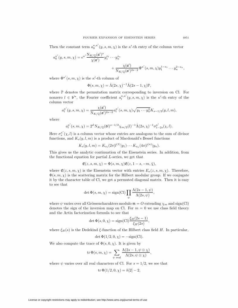
Then the constant term aκ,κ′
0 (y, s,m, χ) is the κ′-th entry of the column vector
aκ′
0 (y, s,m, χ) = eκ′NK/Q(a′)s
χ(a′)ys11 · · · ysnn
+χ(a′)
NK/Q(a′)2s−2Φκ′(s,m, χ)y1−s1
1 · · · y2−snn ,
where Φκ′(s,m, χ) is the κ′-th column of
Φ(s,m, χ) = Λ(2s, χ)−1Λ(2s− 1, χ)P,
where P denotes the permutation matrix corresponding to inversion on Cl. Fornonzero l ∈ b′∗, the Fourier coefficient aκ,κ
′
l (y, s,m, χ) is the κ′-th entry of thecolumn vector
aκ′
l (y, s,m, χ) =χ(a′)
NK/Q(a′)2s−2aκ′
l (s,m, χ)√y1 · · · y2
nKs−1/2(y, l,m),
where
aκ′
l (s,m, χ) = 2d NK/Q(dl)s−1/2χm/2(l)−1Λ(2s, χ)−1σκ′
1−2s(χ, l).
Here σκ′
s (χ, l) is a column vector whose entries are analogous to the sum of divisorfunctions, and Ks(y, l,m) is a product of Macdonald’s Bessel functions
Ks(y, l,m) = Ks1(2π|l(1)|y1) · · ·Ksn(4π|l(n)|yn).
This gives us the analytic continuation of the Eisenstein series. In addition, fromthe functional equation for partial L-series, we get that
E(z, s,m, χ) = Φ(s,m, χ)E(z, 1− s,−m, χ),
where E(z, s,m, χ) is the Eisenstein vector with entries Eκ(z, s,m, χ). Therefore,Φ(s,m, χ) is the scattering matrix for the Hilbert modular group. If we conjugateit by the character table of Cl, we get a permuted diagonal matrix. Then it is easyto see that
det Φ(s,m, χ) = sign(Cl)∏ψ
Λ(2s− 1, ψ)Λ(2s, ψ)
,
where ψ varies over all Grossencharakters modulo m = O extending χm and sign(Cl)denotes the sign of the inversion map on Cl. For m = 0 we use class field theoryand the Artin factorization formula to see that
det Φ(s, 0, χ) = sign(Cl)ξH(2s− 1)ξH(2s)
,
where ξH(s) is the Dedekind ξ-function of the Hilbert class field H . In particular,
det Φ(1/2, 0, χ) = −sign(Cl).
We also compute the trace of Φ(s, 0, χ). It is given by
tr Φ(s,m, χ) =∑ψ real
Λ(2s− 1, ψ ⊗ χ)Λ(2s, ψ ⊗ χ)
,
where ψ varies over all real characters of Cl. For s = 1/2, we see that
tr Φ(1/2, 0, χ) = h[2]− 2,
License or copyright restrictions may apply to redistribution; see http://www.ams.org/journal-terms-of-use

4852 CLAUS MAZANTI SORENSEN
using the analytic properties of Λ(s, ψ) at s = 0, the orthogonality relations forCl /Cl2 and the result of Hecke that [d] ∈ Cl2.
2. The Hilbert modular group and its cusps
Let us recall a few basic facts about hyperbolic 2-space H2 and hyperbolic 3-space H3. We always think of H2 as the upper half-plane of C. Points of H2 aredenoted by z = x+ iy, and we equip H2 with the Poincare metric
ds(z)2 =dx2 + dy2
y2.
The group SL(2,R) acts transitively on H2 by linear fractional transformations,and these are isometries. The isotropy group at i is SO(2), and we obtain a home-omorphism
H2 ≈ SL(2,R)/ SO(2).
From the metric on H2 we obtain a measure that is invariant under the action ofSL(2,R). It is given by
dµ(z) =dxdy
y2.
Similarly, we always think of H3 as the upper half-space C × (0,∞) inside thequaternions. Points of H3 are denoted by z = x + jy, and we put the followingmetric on H3:
ds(z)2 =d|x|2 + dy2
y2.
The group SL(2,C) acts transitively on H3 by linear fractional transformations,and these are isometries. The isotropy group at j is SU(2), and we obtain a home-omorphism
H3 ≈ SL(2,C)/ SU(2).
As before, we obtain a measure dµ(z) on H3 that is invariant under the action ofSL(2,C). It is given by
dµ(z) =dxdy
y3,
where dx is the usual Lebesgue measure on C. In this paper, we consider the space
X = Hr12 ×Hr2
3 .
Points of X are denoted by z = (z1, . . . , zn), where n = r1 + r2. As a productof Riemannian manifolds, the space X has a metric ds(z)2 and a correspondingmeasure dµ(z). The group
G = SL(2,R)r1 × SL(2,C)r2
acts transitively on X by isometries. The isotropy group at the point (i, . . . , j) isthe maximal compact subgroup SO(2)r1×SU(2)r2 , and we obtain a homeomorphismbetween X and the quotient of G by this subgroup. Throughout this paper we fixa number field K with r1 real primes and r2 complex primes. Hence the degree is
d = (K : Q) = r1 + 2r2.
The infinite primes are represented by a certain set of embeddings K → C thatwe also fix. In addition, we put a total order on this set, such that the first r1
License or copyright restrictions may apply to redistribution; see http://www.ams.org/journal-terms-of-use

FOURIER EXPANSION OF EISENSTEIN SERIES 4853
embeddings represent the real primes and the remaining r2 embeddings representthe complex primes. If a ∈ K, we denote by a(i) the i′-th embedding of a. We maylist the embeddings representing the infinite primes:
a(1), . . . , a(r1)︸ ︷︷ ︸r1 real
, a(r1+1), . . . , a(n)︸ ︷︷ ︸r2 complex
,
where n is the number of infinite primes of K. We let O denote the ring of integersin K. Using the embeddings, we may identify SL(2, O) with its image Γ ⊂ G underthe injective homomorphism SL(2,K) ↪→ G defined by(
a bc d
)7→((
a(1) b(1)
c(1) d(1)
), . . . ,
(a(n) b(n)
c(n) d(n)
)).
The image Γ ⊂ G is called the Hilbert modular group associated to the field K. Onecan show that Γ is a discrete, cofinite and irreducible subgroup of G. To explainthe notion of irreducibility, we recall the notion of commensurable groups:
Definition 2.1. Two subgroups Γ ⊂ G and Γ′ ⊂ G are said to be strictly com-mensurable if the intersection Γ ∩ Γ′ has finite index in both Γ and Γ′. They aresaid to be commensurable if Γ′ is strictly commensurable to gΓg−1 for some g ∈ G.
Commensurability and strict commensurability define equivalence relations onthe set of subgroups of G. That Γ is irreducible then means that it is not commen-surable to a direct product Γ1 × Γ2, where Γ1 ⊂ G1 and Γ2 ⊂ G2 are discrete, G1
and G2 are nontrivial and G = G1 × G2. Conversely, in [7] it is shown that anydiscrete cofinite irreducible subgroup of G is commensurable to a Hilbert modulargroup when n > 1. There is a natural left action of G on
P = P1(R)r1 × P1(C)r2 .
The cusps of Γ are, by definition, the parabolic fixpoints in P. It is easy to see thatthe set of cusps is exactly the image of the map P1(K)→ P. The group Γ acts onthe set of cusps, and in fact there are only finitely many inequivalent cusps. Indeed,this number is equal to the ideal class number h.
Proposition 2.2. The number of inequivalent cusps for Γ is equal to h.
Proof. As we have noted, the set of cusps is the image of the map P1(K)→ P. Wethus have a bijection
SL(2, O)\P1(K) ≈ Γ\{cusps}.We are going to establish a bijection between SL(2, O)\P1(K) and the ideal classgroup Cl: Each (a : b) ∈ P1(K) is mapped to the class of the nonzero fractionalideal aO + bO. It is easy to see that this map factors and gives a surjective map
SL(2, O)\P1(K)→ Cl .
To prove that this is injective, look at (a : b) ∈ P1(K) and (a′ : b′) ∈ P1(K) withaO+ bO = a′O+ b′O in Cl. We may assume that aO+ bO = a′O+ b′O = a. Thenwe can find c, d ∈ a−1 and c′, d′ ∈ a−1 such that
σ =(a cb d
)∈ SL(2,K) and σ′ =
(a′ c′
b′ d′
)∈ SL(2,K).
Now we have the following:
(a′, b′)T = σ′(1, 0)T = σ′σ−1(a, b)T ,
License or copyright restrictions may apply to redistribution; see http://www.ams.org/journal-terms-of-use

4854 CLAUS MAZANTI SORENSEN
and by multiplication, we see that σ′σ−1 has entries in O and determinant 1.
The proof gives us a canonical bijection Γ\{cusps} ≈ Cl mapping the class of(a : b) ∈ P1(K) to the ideal class of aO + bO. We will denote by Cκ the idealclass associated to the cusp κ. The following proposition says that we may movean arbitrary cusp κ to ∞ such that the isotropy groups Γκ and Γ∞ are almostconjugate. In many cases, this allows us to consider only the cusp ∞.
Proposition 2.3. Let κ ∈ P be a cusp. Then there exists a σ ∈ SL(2,K) ⊂ Gsuch that σ∞ = κ and
σ−1Γκσ ={(
u b0 u−1
): u ∈ O× and b ∈ a−2
},
for some integral ideal a ∈ Cκ. If σ is another such matrix and a is the correspond-ing ideal, then σ has the form
σ = σ
(a ∗0 a−1
),
where a is a generator of the principal ideal a−1a.
Proof. Write κ = (a : b) where a, b ∈ O and put a = aO + bO. There existsc, d ∈ a−1 such that
σ =(a cb d
)∈ SL(2,K).
Clearly σ∞ = κ. To prove the statement about σ−1Γκσ, consider first a γ ∈ Γκ.Then
σ−1γσ =(u b′
0 u−1
),
for some u ∈ K∗ and b′ ∈ K. By looking at the trace, we conclude that u ∈ O×:
u+ u−1 = tr γ ∈ O ⇒ u, u−1 ∈ O ⇒ u ∈ O×.By computing the upper right entry of σ−1γσ, it is straightforward to verify thatb′ ∈ a−2. Conversely, let u ∈ O× and b′ ∈ a−2. Again, by doing the multiplications,it is straightforward to see that
σ
(u b′
0 u−1
)σ−1
fixes κ, has entries in O and determinant 1. Thus
σ−1Γκσ ={(
u b′
0 u−1
): u ∈ O× and b′ ∈ a
−2
}.
It is also clear that the ideal class of a is the class Cκ associated to κ. This provesthe existence. Now suppose σ is another matrix with the desired properties and leta be the corresponding ideal. Then
σ = σ
(a b′
0 a−1
),
for some a ∈ K∗ and b′ ∈ K. If we use this to express σ−1Γκσ as a conjugate ofσ−1Γκσ, we find that a−2a2 ⊂ (a)2. Doing this the other way around, we find thata−2a2 ⊃ (a)2. By unique factorization, we have a−1a = (a).
License or copyright restrictions may apply to redistribution; see http://www.ams.org/journal-terms-of-use
FOURIER EXPANSION OF EISENSTEIN SERIES 4855
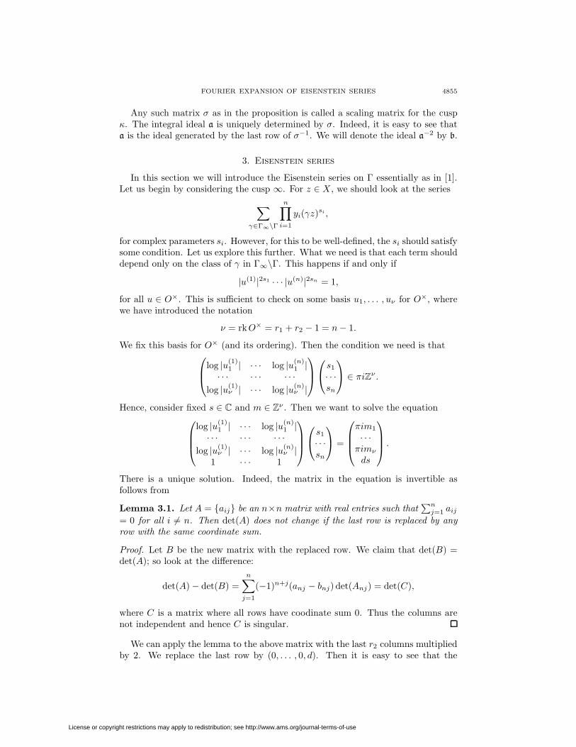
Any such matrix σ as in the proposition is called a scaling matrix for the cuspκ. The integral ideal a is uniquely determined by σ. Indeed, it is easy to see thata is the ideal generated by the last row of σ−1. We will denote the ideal a−2 by b.
3. Eisenstein series
In this section we will introduce the Eisenstein series on Γ essentially as in [1].Let us begin by considering the cusp ∞. For z ∈ X , we should look at the series∑
γ∈Γ∞\Γ
n∏i=1
yi(γz)si ,
for complex parameters si. However, for this to be well-defined, the si should satisfysome condition. Let us explore this further. What we need is that each term shoulddepend only on the class of γ in Γ∞\Γ. This happens if and only if
|u(1)|2s1 · · · |u(n)|2sn = 1,
for all u ∈ O×. This is sufficient to check on some basis u1, . . . , uν for O×, wherewe have introduced the notation
ν = rkO× = r1 + r2 − 1 = n− 1.
We fix this basis for O× (and its ordering). Then the condition we need is thatlog |u(1)1 | · · · log |u(n)
1 |· · · · · · · · ·
log |u(1)ν | · · · log |u(n)
ν |
s1
· · ·sn
∈ πiZν .Hence, consider fixed s ∈ C and m ∈ Zν . Then we want to solve the equation
log |u(1)1 | · · · log |u(n)
1 |· · · · · · · · ·
log |u(1)ν | · · · log |u(n)
ν |1 · · · 1
s1
· · ·sn
=
πim1
· · ·πimν
ds
.
There is a unique solution. Indeed, the matrix in the equation is invertible asfollows from
Lemma 3.1. Let A = {aij} be an n×n matrix with real entries such that∑nj=1 aij
= 0 for all i 6= n. Then det(A) does not change if the last row is replaced by anyrow with the same coordinate sum.
Proof. Let B be the new matrix with the replaced row. We claim that det(B) =det(A); so look at the difference:
det(A)− det(B) =n∑j=1
(−1)n+j(anj − bnj) det(Anj) = det(C),
where C is a matrix where all rows have coodinate sum 0. Thus the columns arenot independent and hence C is singular.
We can apply the lemma to the above matrix with the last r2 columns multipliedby 2. We replace the last row by (0, . . . , 0, d). Then it is easy to see that the
License or copyright restrictions may apply to redistribution; see http://www.ams.org/journal-terms-of-use

4856 CLAUS MAZANTI SORENSEN
determinant of the above matrix is ±2−r2dR where R is the regulator of K. Thuswe may define real numbers eij as follows:
e11 · · · e1ν 1/d· · · · · · · · · · · ·en1 · · · enν 2/d
=
log |u(1)
1 | · · · log |u(n)1 |
· · · · · · · · ·log |u(1)
ν | · · · log |u(n)ν |
1 · · · 1
−1
.
The computation of ein deserves an argument: Let v = (e1n, . . . , enn)T be the lastcolumn. Clearly it is orthogonal to the vectors
vi = (log |u(1)i |, . . . , log |u(n)
i |)T ,
where i = 1, . . . , ν. However, we have just seen that v1, . . . , vν are independent.Clearly, Span{v1, . . . , vν} is contained in the complement of (1, . . . , 2)T . Looking atdimensions we see that Span{v1, . . . , vν} in fact is the complement of (1, . . . , 2)T .Thus v is a multiple of (1, . . . , 2)T , and since 〈v, (1, . . . , 1)T 〉 = 1, we have v =1/d(1, . . . , 2)T . With this notation, the solution to the above equation is given by
si = si(s,m) = s+ πi〈m, ei〉 = s+ πi
ν∑j=1
mjeij
when i ≤ r, where ei is the i′-th row of the left n× ν block of {eij}. When i > r,we must replace s by 2s. Thus the Eisenstein series should have parameters z ∈ X ,s ∈ C, m ∈ Zν and be given as∑
γ∈Γ∞\Γ
n∏i=1
yi(γz)si , where si = si(s,m).
When we consider an arbitrary cusp κ, the Eisenstein series should be∑γ∈Γκ\Γ
n∏i=1
yi(σ−1γz)si , where si = si(s,m),
and σ is a scaling matrix for κ. This still makes sense as a series. However, theseries should not depend on the choice of σ. If σ is another scaling matrix for κ,we have seen that it has the form
σ = σ
(a ∗0 a−1
),
where a is a generator of the principal ideal a−1a. Then (formally at least)∑γ∈Γκ\Γ
n∏i=1
yi(σ−1γz)si =χm(a)
NK/Q(a)2s
∑γ∈Γκ\Γ
n∏i=1
yi(σ−1γz)si ,
where we have introduced the character χm : (R∗)r1 × (C∗)r2 → C1 by
χm(x1, . . . , xn) =n∏i=1
|xi|−2πi〈m,ei〉.
This is trivial on O×, and hence we may consider χm as a character on the groupof principal ideals P . We may extend this character (in h ways) to a character
License or copyright restrictions may apply to redistribution; see http://www.ams.org/journal-terms-of-use
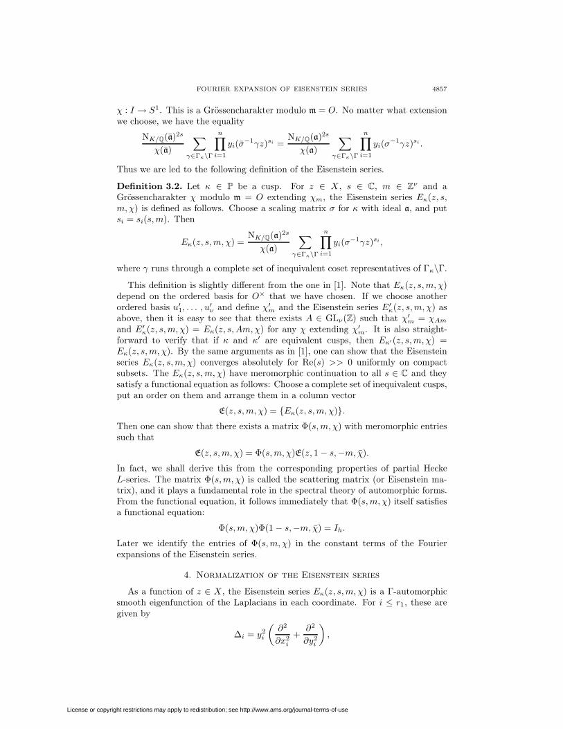
FOURIER EXPANSION OF EISENSTEIN SERIES 4857
χ : I → S1. This is a Grossencharakter modulo m = O. No matter what extensionwe choose, we have the equality
NK/Q(a)2s
χ(a)
∑γ∈Γκ\Γ
n∏i=1
yi(σ−1γz)si =NK/Q(a)2s
χ(a)
∑γ∈Γκ\Γ
n∏i=1
yi(σ−1γz)si .
Thus we are led to the following definition of the Eisenstein series.
Definition 3.2. Let κ ∈ P be a cusp. For z ∈ X , s ∈ C, m ∈ Zν and aGrossencharakter χ modulo m = O extending χm, the Eisenstein series Eκ(z, s,m, χ) is defined as follows. Choose a scaling matrix σ for κ with ideal a, and putsi = si(s,m). Then
Eκ(z, s,m, χ) =NK/Q(a)2s
χ(a)
∑γ∈Γκ\Γ
n∏i=1
yi(σ−1γz)si ,
where γ runs through a complete set of inequivalent coset representatives of Γκ\Γ.
This definition is slightly different from the one in [1]. Note that Eκ(z, s,m, χ)depend on the ordered basis for O× that we have chosen. If we choose anotherordered basis u′1, . . . , u′ν and define χ′m and the Eisenstein series E′κ(z, s,m, χ) asabove, then it is easy to see that there exists A ∈ GLν(Z) such that χ′m = χAmand E′κ(z, s,m, χ) = Eκ(z, s, Am,χ) for any χ extending χ′m. It is also straight-forward to verify that if κ and κ′ are equivalent cusps, then Eκ′(z, s,m, χ) =Eκ(z, s,m, χ). By the same arguments as in [1], one can show that the Eisensteinseries Eκ(z, s,m, χ) converges absolutely for Re(s) >> 0 uniformly on compactsubsets. The Eκ(z, s,m, χ) have meromorphic continuation to all s ∈ C and theysatisfy a functional equation as follows: Choose a complete set of inequivalent cusps,put an order on them and arrange them in a column vector
E(z, s,m, χ) = {Eκ(z, s,m, χ)}.Then one can show that there exists a matrix Φ(s,m, χ) with meromorphic entriessuch that
E(z, s,m, χ) = Φ(s,m, χ)E(z, 1− s,−m, χ).
In fact, we shall derive this from the corresponding properties of partial HeckeL-series. The matrix Φ(s,m, χ) is called the scattering matrix (or Eisenstein ma-trix), and it plays a fundamental role in the spectral theory of automorphic forms.From the functional equation, it follows immediately that Φ(s,m, χ) itself satisfiesa functional equation:
Φ(s,m, χ)Φ(1 − s,−m, χ) = Ih.
Later we identify the entries of Φ(s,m, χ) in the constant terms of the Fourierexpansions of the Eisenstein series.
4. Normalization of the Eisenstein series
As a function of z ∈ X , the Eisenstein series Eκ(z, s,m, χ) is a Γ-automorphicsmooth eigenfunction of the Laplacians in each coordinate. For i ≤ r1, these aregiven by
∆i = y2i
(∂2
∂x2i
+∂2
∂y2i
),
License or copyright restrictions may apply to redistribution; see http://www.ams.org/journal-terms-of-use

4858 CLAUS MAZANTI SORENSEN
while for i > r1, they are given by
∆i = y2i
(∂2
∂xi∂xi+
∂2
∂y2i
)− yi
∂
∂yi.
They are clearly invariant. A general theorem says that a diffeomorphism of aRiemannian manifold is an isometry if and only if it leaves the Laplace operatorinvariant. They are the fundamental operators in the terminology of [6]. We wantto study the asymptotics of Eκ(z, s,m, χ) as z → κ′ within a fundamental domain.We do this by choosing a scaling matrix σ′ for κ′, and look at Eκ(σ′z, s,m, χ)as z → ∞. Only the dependence of y = (y1, . . . , yn) ∈ Rn+ is important, sincex = (x1, . . . , xn) ∈ Rr1 × Cr2 is bounded within a fundamental domain. Thus wefix a y ∈ Rn+, and look at Eκ(σ′z, s,m, χ) as a function of x ∈ Rr1 × Cr2 . SinceEisenstein series are automorphic, we find that it is b′-periodic where b′ is the idealof σ′ thought of as a complete lattice in Rr1×Cr2 . Hence it has a Fourier expansion
Eκ(σ′z, s,m, χ) =∑l∈b′∗
aκ,κ′
l (y, s,m, χ)e2πiTrK/Q(lx),
where b′∗ = {l ∈ K : TrK/Q(lb′) ⊂ Z} is the dual module and
TrK/Q(x) =∑i≤r1
xi +∑i>r1
2 Re(xi)
for x = (x1, . . . , xn) ∈ Rr1 × Cr2 . The Fourier coefficients are given by
aκ,κ′
l (y, s,m, χ) =2r2
NK/Q(b′)√|D|
∫Fb′
Eκ(σ′z, s,m, χ)e−2πiTrK/Q(lx)dx,
where Fb′ is a fundamental mesh for the lattice, D is the discriminant of K anddx is the usual Lebesgue measure on Rr1 × Cr2 . We use this notation, keeping inmind that aκ,κ
′
l (y, s,m, χ) depends on the choice of a scaling matrix
σ′ =(a′ c′
b′ d′
)∈ SL(2,K) ⊂ G
for κ′. The main result of this paper is the computation of the Fourier coefficientsabove.
Lemma 4.1. Let σ be a scaling matrix for κ with ideal a. Then
Eκ(σ′z, s,m, χ) =NK/Q(a)2s
χ(a)
∑(C,D)×
(Cd′−Db′,Cc′−Da′)=a
n∏i=1
ysii|C(i)zi +D(i)|2si
where (C,D)× denotes O×-equivalence.
Proof. Note that the group σ−1Γκσ acts on the set σ−1Γσ′, and we can write
Eκ(σ′z, s,m, χ) =NK/Q(a)2s
χ(a)
∑γ∈σ−1Γκσ\σ−1Γσ′
n∏i=1
yi(γz)si .
The map that associates the last row to a γ ∈ σ−1Γσ′ factors and gives a bijection
σ−1Γκσ\σ−1Γσ′ ≈{
Pairs (C,D) of C,D ∈ Ks.t. (A,B,C,D) ∈ σ−1Γσ′
for some A,B ∈ K
}/O×.
License or copyright restrictions may apply to redistribution; see http://www.ams.org/journal-terms-of-use

FOURIER EXPANSION OF EISENSTEIN SERIES 4859
Thus, we may write
Eκ(σ′z, s,m, χ) =NK/Q(a)2s
χ(a)
∑(C,D)×
(A,B,C,D)∈σ−1Γσ′
n∏i=1
ysii|C(i)zi +D(i)|2si .
Now, from the section on the cusps we know that
∃A,B :(A BC D
)∈ σ−1Γσ′ ⇔ (Cd′ −Db′, Cc′ −Da′) = a,
since a is the ideal generated by the last row of σ−1.
Let us briefly recall the definition of the partial L-series L(s, χ, C), where χ :I→S1 is a Grossencharakter modulo m = O extending χm, and C ∈ Cl is an idealclass:
L(s, χ, C) =∑a∈C
integral
χ(a)NK/Q(a)s
.
The series is absolutely convergent for Re(s) > 1, and uniformly in Re(s) > 1 + εfor every ε > 0. Thus L(s, χ, C) defines an analytic function for Re(s) > 1. Wedefine the completed partial L-series by
Λ(2s, χ, C) = 2r2+(s1+···+sr1 )(2π)−ds|D|s{
n∏i=1
Γ(si)
}L(2s, χ, C),
where si = si(s,m). It is shown in [5] that Λ(s, χ, C) has a meromorphic continu-ation to the whole complex plane, and a functional equation
Λ(s, χ, C) = χ(d)Λ(1 − s, χ, C′),where CC′ = [d], is the class of the different d. Recall that, by definition, d−1 = O∗.We fix a complete set of inequivalent cusps, put an order on it and arrange thepartial L-series in an h× h matrix as follows:
L(s, χ) = {L(s, χ, C−1κ Cκ′)}.
We also fix scaling matrices for each of the cusps, and put
E(z, s,m, χ) = {Eκ(σ′z, s,m, χ)}.We always assume that ∞ is in our set of inequivalent cusps, and that the fixed
scaling matrix there is 1. Then we have the following analogue of Proposition 2.5in [2]:
Lemma 4.2. Let σ be a scaling matrix for κ with ideal a. Then
(L(2s, χ)E(z, s,m, χ))κκ′ =NK/Q(a)2s
χ(a)
∑(C,D)×
06=(Cd′−Db′,Cc′−Da′)⊂a
n∏i=1
ysii|C(i)zi +D(i)|2si
where (C,D)× denotes O×-equivalence.
Proof. The right-hand side is equal to
NK/Q(a)2s
χ(a)
∑a|q
∑(C,D)×
(Cd′−Db′,Cc′−Da′)=q
n∏i=1
ysii|C(i)zi +D(i)|2si .
License or copyright restrictions may apply to redistribution; see http://www.ams.org/journal-terms-of-use

4860 CLAUS MAZANTI SORENSEN
We divide the first sum into ideal classes and obtain
NK/Q(a)2s
χ(a)
∑κ′′
∑a|q
q∈Cκ′′
∑(C,D)×
(Cd′−Db′,Cc′−Da′)=q
n∏i=1
ysii|C(i)zi +D(i)|2si ,
where κ′′ runs through the complete set of inequivalent cusps. Writing q as q =a′′(θ), where θ ∈ a′′−1a, we find that this equals
NK/Q(a)2s
χm(a)
∑κ′′
∑(θ) 6=0
θ∈a′′−1
a
∑(C,D)×
(Cd′−Db′,Cc′−Da′)=a′′(θ)
n∏i=1
ysii|C(i)zi +D(i)|2si .
Changing variables C → C/θ and D → D/θ, we get
NK/Q(a)2s
χ(a)
∑κ′′
∑(θ) 6=0
θ∈a′′−1
a
χ(θ)NK/Q(θ)2s
∑(C,D)×
(Cd′−Db′,Cc′−Da′)=a′′
n∏i=1
ysii|C(i)zi +D(i)|2si .
Using the lemma above, and the fact that a−1a′′(θ) runs through all integral idealsin the class C−1
κ Cκ′′ as θ ∈ a′′−1a, we see that this is equal to the left-hand side.
As we see from Lemma 4.1, the Eisenstein series can be written as
Eκ(z, s,m, χ) =NK/Q(a)2s
χ(a)
∑(C,D)×
(C,D)=a
n∏i=1
ysii|C(i)zi +D(i)|2si .
We define the normalized Eisenstein series to be
E∗κ(z, s,m, χ) =NK/Q(a)2s
χ(a)
∑(C,D)×
06=(C,D)⊂a
n∏i=1
ysii|C(i)zi +D(i)|2si .
From Lemma 4.2, it follows that
E∗(z, s,m, χ) = L(2s, χ)E(z, s,m, χ),
where E∗(z, s,m, χ) is the matrix with entries E∗κ(σ′z, s,m, χ). We also define thecompleted Eisenstein series to be
Eκ(z, s,m, χ) = 2r2+(s1+···+sr1)(2π)−ds|D|s{
n∏i=1
Γ(si)
}E∗κ(z, s,m, χ).
Then we have the identity
E(z, s,m, χ) = Λ(2s, χ)E(z, s,m, χ),
where E(z, s,m, χ) is the matrix with entries Eκ(σ′z, s,m, χ), and
Λ(s, χ) = {Λ(s, χ, C−1κ Cκ′)}.
In particular, Eκ(σ′z, s,m, χ) is b′-periodic. We compute the Fourier expansion ofit, and from this we get the Fourier expansion of Eκ(σ′z, s,m, χ).
License or copyright restrictions may apply to redistribution; see http://www.ams.org/journal-terms-of-use
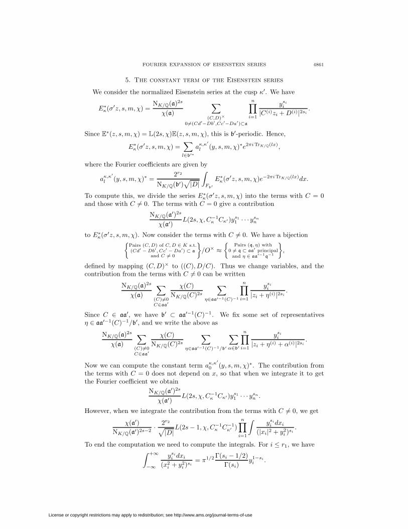
FOURIER EXPANSION OF EISENSTEIN SERIES 4861
5. The constant term of the Eisenstein series
We consider the normalized Eisenstein series at the cusp κ′. We have
E∗κ(σ′z, s,m, χ) =NK/Q(a)2s
χ(a)
∑(C,D)×
06=(Cd′−Db′,Cc′−Da′)⊂a
n∏i=1
ysii|C(i)zi +D(i)|2si .
Since E∗(z, s,m, χ) = L(2s, χ)E(z, s,m, χ), this is b′-periodic. Hence,
E∗κ(σ′z, s,m, χ) =∑l∈b′∗
aκ,κ′
l (y, s,m, χ)∗e2πiTrK/Q(lx),
where the Fourier coefficients are given by
aκ,κ′
l (y, s,m, χ)∗ =2r2
NK/Q(b′)√|D|
∫Fb′
E∗κ(σ′z, s,m, χ)e−2πiTrK/Q(lx)dx.
To compute this, we divide the series E∗κ(σ′z, s,m, χ) into the terms with C = 0and those with C 6= 0. The terms with C = 0 give a contribution
NK/Q(a′)2s
χ(a′)L(2s, χ, C−1
κ Cκ′)ys11 · · · ysnn
to E∗κ(σ′z, s,m, χ). Now consider the terms with C 6= 0. We have a bijection{Pairs (C,D) of C,D ∈ K s.t.(Cd′ −Db′, Cc′ −Da′) ⊂ a
and C 6= 0
}/O× ≈
{Pairs (q, η) with
0 6= q ⊂ aa′ principal
and η ∈ aa′−1
q−1
},
defined by mapping (C,D)× to ((C), D/C). Thus we change variables, and thecontribution from the terms with C 6= 0 can be written
NK/Q(a)2s
χ(a)
∑(C) 6=0C∈aa
′
χ(C)NK/Q(C)2s
∑η∈aa′−1(C)−1
n∏i=1
ysii|zi + η(i)|2si .
Since C ∈ aa′, we have b′ ⊂ aa′−1(C)−1. We fix some set of representativesη ∈ aa′−1(C)−1/b′, and we write the above as
NK/Q(a)2s
χ(a)
∑(C) 6=0C∈aa
′
χ(C)NK/Q(C)2s
∑η∈aa′−1(C)−1/b′
∑α∈b′
n∏i=1
ysii|zi + η(i) + α(i)|2si .
Now we can compute the constant term aκ,κ′
0 (y, s,m, χ)∗. The contribution fromthe terms with C = 0 does not depend on x, so that when we integrate it to getthe Fourier coefficient we obtain
NK/Q(a′)2s
χ(a′)L(2s, χ, C−1
κ Cκ′)ys11 · · · ysnn .
However, when we integrate the contribution from the terms with C 6= 0, we get
χ(a′)NK/Q(a′)2s−2
· 2r2√|D|
L(2s− 1, χ, C−1κ C−1
κ′ )n∏i=1
∫ysii dxi
(|xi|2 + y2i )si
.
To end the computation we need to compute the integrals. For i ≤ r1, we have∫ +∞
−∞
ysii dxi(x2i + y2
i )si= π1/2 Γ(si − 1/2)
Γ(si)y1−sii .
License or copyright restrictions may apply to redistribution; see http://www.ams.org/journal-terms-of-use
4862 CLAUS MAZANTI SORENSEN
See for example [4]. The case i > r1 is much easier:∫ 2π
0
dθi
∫ ∞0
ysii ridri(r2i + y2
i )si=
π
si − 1y2−sii .
Thus the contribution to ∗aκ,κ′
0 (y, s,m, χ) from the terms with C 6= 0 is
χ(a′)NK/Q(a′)2s−2
· 2r2πd2√|D|
∏i≤r1
Γ(si − 12 )
Γ(si)
∏i>r1
1si − 1
× L(2s− 1, χ, C−1
κ C−1κ′ )y1−s1
1 · · · y2−snn .
Thus we have computed ∗aκ,κ′
0 (y, s,m, χ). We rewrite this in terms of the completedpartial L-series. It is easy to see that for any ideal class C,
Λ(2s− 1, χ, C)Λ(2s, χ, C)
=2r2πd/2√|D|
∏i≤r1
Γ(si − 1/2)Γ(si)
∏i>r1
1si − 1
L(2s− 1, χ, C)L(2s, χ, C)
.
If we let aκ,κ′
0 (y, s,m, χ) denote the constant term of Eκ(σ′z, s,m, χ), then theabove shows that it is a sum of a contribution
NK/Q(a′)2s
χ(a′)Λ(2s, χ, C−1
κ Cκ′)ys11 · · · ysnn
and a contribution from the terms with C 6= 0 given by
χ(a′)NK/Q(a′)2s−2
· Λ(2s− 1, χ, C−1κ C−1
κ′ )y1−s11 · · · y2−sn
n .
To get aκ,κ′
0 (y, s,m, χ), we interpret the above as a matrix equation. We arrangeall the constant terms in a matrix
a0(y, s,m, χ) = {aκ,κ′
0 (y, s,m, χ)},and similarly we define a0(y, s,m, χ). We let P denote the permutation matrixcorresponding to inversion on Cl,
P = {δκι(κ′)},where ι is the permutation of the {κ} corresponding to inversion on the class group:
Cι(κ) = C−1κ .
Then what we have proved above is the following
Lemma 5.1. Let κ′ be a fixed cusp. The constant terms are given by
aκ′
0 (y, s,m, χ) = eκ′NK/Q(a′)s
χ(a′)ys11 · · · ysnn +
χ(a′)NK/Q(a′)2s−2
Φκ′(s,m, χ)y1−s1
1 · · · y2−snn
where Φκ′(s,m, χ) is the κ′-th column of
Φ(s,m, χ) = Λ(2s, χ)−1Λ(2s− 1, χ)P,
with notation as above.
Later, when we have computed the remaining terms of the Eisenstein series, wefind that the matrix Φ(s,m, χ), in fact, is the scattering matrix.
License or copyright restrictions may apply to redistribution; see http://www.ams.org/journal-terms-of-use

FOURIER EXPANSION OF EISENSTEIN SERIES 4863
6. The remaining terms of the Eisenstein series
We now compute the Fourier coefficients aκ,κ′
l (y, s,m, χ)∗ for nonzero l ∈ b′∗.As before we divide the series E∗κ(σ′z, s,m, χ) into the terms with C = 0 and thosewith C 6= 0. The terms with C = 0 give no contribution. The other terms give
χ(a′)NK/Q(a′)2s−2
· 2r2√|D|
σκ,κ′
1−2s(χ, l)∫ n∏
i=1
ysii e−2πiTrK/Q(lx)
(|xi|2 + y2i )si
dx,
where we have introduced the notation
σκ,κ′
s (χ, l) =∑
q∈C−1κ C−1
κ′integralq|b′dl
χ(q) NK/Q(q)s.
To see this, note that a∗ = a−1O∗. Note also that b′dl is integral. In particular,this sum is finite. The integral equals{∫ +∞
−∞
ys11 e−2πil(1)x1dx1
(x21 + y2
1)s1
}· · ·{∫
C
ysnn e−4πiRe(l(n)xn)dxn(|xn|2 + y2
n)sn
}.
Using the well-known result that∫ +∞
−∞
e−2πiAt
(1 + t2)sdt =
2πs|A|s−1/2Ks−1/2(2π|A|)Γ(s)
,
see for example [4], it follows that for i ≤ r1, we have∫ +∞
−∞
ysii e−2πil(i)xidxi
(x2i + y2
i )si=
2πsi |l(i)|si−1/2√yiKsi−1/2(2π|l(i)|yi)Γ(si)
.
To compute the last r2 factors, we apply the following integral:∫ +∞
−∞
∫ +∞
−∞
e−2πi(Au−Bv)
(1 + u2 + v2)sdudv =
2πs|C|s−1Ks−1(2π|C|)Γ(s)
,
where A2 + B2 = C2. To prove this, make a linear change of variables and applythe integral above. Then for i > r1, we have∫
C
ysii e−4πiRe(l(i)xi)dxi(|xi|2 + y2
i )si=
(2π)si |l(i)|si−1yiKsi−1(4π|l(i)|yi)Γ(si)
.
Now we can put all this together and obtain an expression for aκ,κ′
l (y, s,m, χ)∗.The best way to state the result is that
aκ,κ′
l (y, s,m, χ) =χ(a′)
NK/Q(a′)2s−2
· 2d NK/Q(dl)s−1/2χm/2(l)−1σκ,κ′
1−2s(χ, l)√y1 · · · y2
nKs−1/2(y, l,m),
where d is the different,
χm/2(l) =n∏i=1
|l(i)|−πi〈m,ei〉,
and
Ks(y, l,m) = Ks1(2π|l(1)|y1) · · ·Ksn(4π|l(n)|yn).
License or copyright restrictions may apply to redistribution; see http://www.ams.org/journal-terms-of-use

4864 CLAUS MAZANTI SORENSEN
To get aκ,κ′
l (y, s,m, χ), we arrange them in a column vector
aκ′
l (y, s,m, χ) = {aκ,κ′
l (y, s,m, χ)},
and similarly we define aκ′
l (y, s,m, χ). We also put
σκ′
s (χ, l) = {σκ,κ′
s (χ, l)}.Then what we have shown is the following
Lemma 6.1. Let κ′ be a fixed cusp. For a nonzero l ∈ b′∗, we have
aκ′
l (y, s,m, χ) =χ(a′)
NK/Q(a′)2s−2aκ′
l (s,m, χ)√y1 · · · y2
nKs−1/2(y, l,m),
where
aκ′
l (s,m, χ) = 2d NK/Q(dl)s−1/2χm/2(l)−1Λ(2s, χ)−1σκ′
1−2s(χ, l)
with notation as above.
7. The scattering matrix
In the previous two sections, we have computed the Fourier expansion of theEisenstein vector E(z, s,m, χ) around a cusp κ′. We have
E(σ′z, s,m, χ) =∑l∈b′∗
aκ′
l (y, s,m, χ)e2πiTrK/Q(lx),
where the constant term is
aκ′
0 (y, s,m, χ) = eκ′NK/Q(a′)s
χ(a′)ys11 · · · ysnn +
χ(a′)NK/Q(a′)2s−2
Φκ′(s,m, χ)y1−s1
1 · · · y2−snn
where Φκ′(s,m, χ) is the κ′-th column of
Φ(s,m, χ) = Λ(2s, χ)−1Λ(2s− 1, χ)P.
For nonzero l ∈ b′∗, the Fourier coefficients are
aκ′
l (y, s,m, χ) =χ(a′)
NK/Q(a′)2s−2aκ′
l (s,m, χ)√y1 · · · y2
nKs−1/2(y, l,m),
where
aκ′
l (s,m, χ) = 2d NK/Q(dl)s−1/2χm/2(l)−1Λ(2s, χ)−1σκ′
1−2s(χ, l).
Let us put κ′ =∞. Using the exponential decay of Macdonald’s Bessel function andthe meromorphic continuation of partial Hecke L-series, we see that this gives themeromorphic continuation of the Eisenstein series. Using the functional equation ofpartial Hecke L-series, we shall now derive the functional equation of the Eisensteinvector. First we check that
Φ(s,m, χ)Φ(1 − s,−m, χ) = Ih.
This follows immediately from the relation
Λ(s, χ)P = χ(d)PdΛ(1− s, χ),
where Pd is the permutation matrix
Pd = {δπ(κ),κ′},
License or copyright restrictions may apply to redistribution; see http://www.ams.org/journal-terms-of-use

FOURIER EXPANSION OF EISENSTEIN SERIES 4865
and where π is the permutation of the {κ} given by
C−1π(κ) = [d]Cκ.
Macdonald’s Bessel functions are even in the s variable, and hence
K−s(y, l,−m) = Ks(y, l,m).
The last relation we need in order to prove the functional equation is
Lemma 7.1. Pdσκ′
s (χ, l) = NK/Q(b′dl)sχ(b′dl)σκ′
−s(χ, l).
Proof. By definition of π, we see that
(Pdσκ′
s (χ, l))κ =∑
q∈[d]CκC−1κ′
integralq|b′dl
χ(q) NK/Q(q)s.
There is a bijection {q ∈ [d]CκC
−1κ′
integralq|b′dl
}≈{
q ∈ C−1κ C−1
κ′integralq|b′dl
},
given by q 7→ q−1b′dl. Hence,
(Pdσκ′
s (χ, l))κ =∑
q∈C−1κ C−1
κ′integralq|b′dl
χ(q−1b′dl) NK/Q(q−1
b′dl)s,
and the claim follows immediately.
Now a straightforward calculation gives us the functional equation
E(z, s,m, χ) = Φ(s,m, χ)E(z, 1− s,−m, χ).
Thus we have finally identified the scattering matrix.
Theorem 7.2. The scattering matrix for the Hilbert modular group is
Φ(s,m, χ) = Λ(2s, χ)−1Λ(2s− 1, χ)P,
with notation as above.
8. The scattering determinant
In this section, we compute the scattering determinant det Φ(s,m, χ) in terms ofHecke L-series. In order to do so, we must compute det Λ(s, χ). For this purpose,we have the following well-known result:
Proposition 8.1. Let G be a finite abelian group, and f any function. Then
deta,b
f(a−1b) =∏ψ∈G∗
∑a∈G
ψ(a)f(a),
where G∗ = {ψ} is the group of characters.
License or copyright restrictions may apply to redistribution; see http://www.ams.org/journal-terms-of-use

4866 CLAUS MAZANTI SORENSEN
Proof. Let X(G) denote the |G|-dimensional complex vector space of functions onG. It has two canonical bases:
(1) the characters {ψ : ψ ∈ G∗},
(2) the functions {δb : b ∈ G} where δb(x) = δx,b.
For each a ∈ G, we have the linear map Ta on X(G) defined by Taf(x) = f(ax).We weight all these Ta using f and consider the linear map
T =∑a∈G
f(a−1)Ta.
To derive the Dedekind determinant relation, we compute detT using the twocanonical bases. It is clear that
Tψ =
{∑a∈G
ψ(a)f(a−1)
}ψ,
for every ψ ∈ G∗. Hence the first basis is a basis of eigenvectors, so that
detT =∏ψ∈G∗
∑a∈G
ψ(a)f(a−1) =∏ψ∈G∗
∑a∈G
ψ(a)f(a).
On the other hand, a straightforward computation shows that
Tδb =∑a∈G
f(a−1b)δa.
Thus we also have
detT = deta,b
f(a−1b).
Comparing these two expressions for detT finishes the proof.
Using this proposition, we can now proceed with our calculation. It follows that
det Λ(s, χ) =∏ψ∈Cl∗
Λ(s, ψ ⊗ χ).
As ψ varies over Cl∗, the product ψ ⊗ χ varies over all Grossencharakters modulom = O extending χm. We thus have
Corollary 8.2. The scattering determinant for the Hilbert modular group is
det Φ(s,m, χ) = sign(Cl)∏ψ
Λ(2s− 1, ψ)Λ(2s, ψ)
,
where ψ varies over all Grossencharakters modulo m = O extending χm.
As we see, det Φ(s,m, χ) does not depend on χ; so we use the notation
φ(s,m) = det Φ(s,m, χ).
In the corollary, sign(Cl) denotes the sign of the inversion map on Cl. This is givenby
sign(Cl) = (−1)(h−h[2])/2,
where h[2] = ]Cl[2]. In the case where K is an imaginary quadratic field (as in [2]),the 2-torsion h[2] can be expressed via genus theory as
h[2] = 2t−1, where t is the number of primes dividing D.
License or copyright restrictions may apply to redistribution; see http://www.ams.org/journal-terms-of-use

FOURIER EXPANSION OF EISENSTEIN SERIES 4867
See for example [3]. We now consider the particularly interesting case where m = 0.Then
φ(s, 0) = sign(Cl)∏ψ∈Cl∗
Λ(2s− 1, ψ)Λ(2s, ψ)
,
and via class field theory, we can interpret this in terms of the Hilbert class field
H = the maximal unramified abelian extension of K.
Here unramified means everywhere unramified, also at the infinite places (so realplaces stay real). The Artin map induces an isomorphism
r : Cl ≈ Gal(H/K)
mapping p 7→ Frp. It is known that the Artin L-function
Λ(s, ψ ◦ r−1, H/K) = Λ(s, ψ).
See for example [5]. Then the Artin factorization formula gives
ξH(s) =∏ψ∈Cl∗
Λ(s, ψ),
where ξH(s) is the Dedekind ξ-function of H . Recall that for a number field K, wehave
ξK(s) = 2r2(1−s)π−ds/2|D|s/2Γ(s/2)r1Γ(s)r2ζK(s).
This satisfies the functional equation ξK(1 − s) = ξK(s). Since H is everywhereunramified, real places stay real; so the Dedekind ξ-function of H is then given by
ξH(s) = 2hr2(1−s)π−hds/2|DH |s/2Γ(s/2)hr1Γ(s)hr2ζH(s).
Then what we have shown is the following
Corollary 8.3. For m = 0, the scattering determinant is given by
φ(s, 0) = sign(Cl)ξH(2s− 1)ξH(2s)
,
with notation as above.
Using this corollary, we can give the following analytic interpretation of sign(Cl)in terms of the central critical value of φ(s, 0):
Corollary 8.4. φ(1/2, 0) = −sign(Cl).
Proof. It is a fact that the only poles of ξH(s) are s = 0 and s = 1. They are knownto be simple, and their residues are given as follows:
Ress=0 ξH(s) = −2hr1hHRHwH
and Ress=1 ξH(s) = +2hr1hHRH
wH.
For the proof of these facts, see [5]. Then we have
φ(s/2, 0) = sign(Cl)(s− 1)ξH(s− 1)
(s− 1)ξH(s)→− sign(Cl),
as s→1. Hence φ(1/2, 0) = −sign(Cl) as we claimed.
License or copyright restrictions may apply to redistribution; see http://www.ams.org/journal-terms-of-use

4868 CLAUS MAZANTI SORENSEN
9. The scattering trace
In this section, we compute the scattering trace tr Φ(s,m, χ) in terms of HeckeL-series. To compute the trace of
Φ(s,m, χ) = Λ(2s, χ)−1Λ(2s− 1, χ)P,
we diagonalize Λ(s, χ). From the proof of the Dedekind determinant, we get that
Λ(s, χ) = M−1 diag(. . . ,Λ(s, ψ ⊗ χ), . . . )M,
where M is the unitary matrix given by the character table
M ={
1√hψ(Cκ)
}.
It follows from this that we may write the scattering matrix as
Φ(s,m, χ) = M−1 diag(. . . ,Λ(2s− 1, ψ ⊗ χ)
Λ(2s, ψ ⊗ χ), . . . )PMM,
where PM = MPM−1. Using the fact that M is unitary and the orthogonalityrelations, we see that PM is the permutation matrix corresponding to inversion onCl∗. From this the following corollary follows immediately.
Corollary 9.1. The scattering trace for the Hilbert modular group is
tr Φ(s,m, χ) =∑ψ real
Λ(2s− 1, ψ ⊗ χ)Λ(2s, ψ ⊗ χ)
,
where ψ varies over all real characters of Cl.
We want to compute the central scattering trace tr Φ(1/2, 0, χ), the main moti-vation being that (at least for totally real fields) it occurs in the trace formula. See[1]. From the functional equation, it follows that for real χ we have
tr Φ(1/2, 0, χ) =∑ψ real
(−1)mψψ(d),
where mψ is the order of vanishing of Λ(s, ψ) at s = 0. By the work of Hecke andTate we know that Λ(s, ψ) is entire if ψ 6= 1. By the Artin factorization formula andthe computation of residues for Dedekind ξ-functions, we thus see that mψ = 0 ifψ 6= 1. If on the other hand ψ = 1, we know that mψ = −1. Using the orthogonalityrelations for the group Cl /Cl2, it follows that
tr Φ(1/2, 0, χ) = h[2]− 2,
when [d] ∈ Cl2. It is a result of Hecke that this condition is always satisfied. Thuswe have
Corollary 9.2. For real χ the central scattering trace is given by
tr Φ(1/2, 0, χ) = h[2]− 2,
with notation as above.
When K is quadratic imaginary, we can rewrite this via genus theory and obtainthe expression in [2]. We note that we can easily derive the formula
φ(1/2, 0) = −sign(Cl)
License or copyright restrictions may apply to redistribution; see http://www.ams.org/journal-terms-of-use

FOURIER EXPANSION OF EISENSTEIN SERIES 4869
from the above. Let A = Φ(1/2, 0, χ). Then A2 = Ih and hence it has eigenvalues±1. Let m± be the multiplicities. Then we have
m+ +m− = h and m+ −m− = h[2]− 2.
From this it follows that
m+ = 12 (h+ h[2]− 2) and m− = 1
2 (h− h[2] + 2),
and we see that detA = (−1)m− = − sign(Cl).
References
1. Efrat, Isaac Y., The Selberg trace formula for PSL2(R)n, Mem. Amer. Math. Soc. 65 (1987),no. 359, iv+111 pp. MR 88e:11041
2. Efrat, I. and Sarnak, P., The determinant of the Eisenstein matrix and Hilbert class fields,Trans. Amer. Math. Soc. 290 (1985), no. 2, 815–824. MR 87b:11039
3. Janusz, Gerald J., Algebraic number fields, Pure and Applied Mathematics, Vol. 55. AcademicPress [A Subsidiary of Harcourt Brace Jovanovich, Publishers], New York-London, 1973. x+220pp. MR 51:3110
4. Kubota, Tomio, Elementary theory of Eisenstein series, Kodansha Ltd., Tokyo; Halsted Press[John Wiley and Sons], New York-London-Sydney, 1973. xi+110 pp. MR 55:2759
5. Neukirch, Jurgen, Algebraic number theory, Translated from the 1992 German original and witha note by Norbert Schappacher. With a foreword by G. Harder. Grundlehren der Mathematis-chen Wissenschaften [Fundamental Principles of Mathematical Sciences], 322. Springer-Verlag,Berlin, 1999. xviii+571 pp. MR 2000m:11104
6. Selberg, A., Harmonic analysis and discontinuous groups in weakly symmetric Riemannianspaces with applications to Dirichlet series, J. Indian Math. Soc. (N.S.) 20 (1956), 47–87. MR19:531g
7. Selberg, Atle, Recent developments in the theory of discontinuous groups of motions of sym-metric spaces, 1970 Proceedings of the Fifteenth Scandinavian Congress (Oslo, 1968), LectureNotes in Mathematics, Vol. 118 Springer, Berlin, pp. 99–120 MR 41:8595
Department of Mathematics, Ny Munkegade, 8000 Aarhus C, Denmark
E-mail address: [email protected]
Current address: Department of Mathematics, California Institute of Technology, Pasadena,California 91125, USA
License or copyright restrictions may apply to redistribution; see http://www.ams.org/journal-terms-of-use