Formerly Lecture 12 now Lecture 10: Introduction to Remote Sensing and Atmospheric Correction*...

Formerly Lecture 12 now Lecture 10:

Introduction to Remote Sensing and Atmospheric Correction*

Collin Roesler11 July 2007

*A 30 min summary of the highlights of Howard Gordon’s 9hr

Short course Ocean Optics XVI 2002Do not use any of the figures for any public presentation without Howard’s permission

1970’s Jerlov Kd Classification

Type Kd(440) Chl .I 0.017 0.01…III 0.14 2.00

1 0.20 >2.00…9 1.0 >10.00

Variability attributed primarily to chlorophyll.Suggested that the inverse problem to estimateChlorophyll from Lu() should be tractable.

0

0.2

0.5

0.9

1.6

inf

1970 Clarke, Ewing, Lorenzen

Chl<0.1

0.31.33.0

• aircraft-based radiometer (305 m)

• Sargasso to WHOI• vertically polarized

light• 53o (Brewster’s Angle)

to avoid skylight

Blue to green ratioDecreased with chl

Coastal Zone Color Scanner

• launched in Nov 1978• proposed mission was 1 year• proof of concept• degraded over time (mirrors)• lasted until 1986


955 km

825 m pixels res.


measured by sensor

atmospheric radiance

water-leaving radiance

reflected radiance

The atmosphere contributes > 90% to the radiance detected by the satellite-based sensor

The Problem

measured by sensor



reflected radiance

1% error in atmospheric correction or satellite calibration 10% error in water leaving radiance

The atmosphere contributes > 90% to the radiance detected by the satellite-based sensor

The Problem

measured by sensor



reflected radiance

Atmospheric CorrectionCZCS Gordon and Clark 1981 First order correction, clear waterSeaWiFS Wang and Gordon 1994 Gordon 1997

What is being measured by the satellite sensor?

• Path radiance, L*– molecular scattering– aerosol scattering– molecular-aerosol

multiple scattering

• white caps, Lwc

• sun glint, Lg

• water leaving radiance, Lw

Remotely sensed radiance equation

Lt = L*r + L*a + L*ra + TLg + tLwc + tLw

• L*r, Rayleigh molecular scattering,

• L*a, Aerosol scattering

• L*ra, Rayleigh-Aerosol multiple scattering

• Lg, sun glint

• Lwc, white caps

• Lw, water leaving radiance

• T, direct transmittance (~beam attenuation)• t, diffuse transmittance

1. Atmospheric Effects (L*, T, t)

• Gaseous absorption (ozone, water vapor, oxygen)

• Scattering by air molecules (Rayleigh)

• Scattering and absorption by aerosols (haze, dust, pollution)

• Polarization (MODIS response varies w/ signal polarization)

Rayleigh (80-85% of total signal)• small molecules compared to nm

wavelength, scattering efficiency decreases with wavelength as -4

• reason for blue skies and red sunsets

• can be accurately approximated for a given atmospheric pressure and geometry (using a radiative transfer code)

Aerosols (0-10% of total signal)

• particles comparable in size to the wavelength of light, scattering is a complex function of particle size

• whitens or yellows the sky

• significantly varies and cannot be easily approximated

1. Atmospheric Effects

Direct Transmittance

T Lsun(top of atmosphere) = e- is the optical depth Lsun(bottom of atm)

%T

0.190

0.375

1.037

2.014

1. Atmospheric EffectsA. Absorption (T)

Ozone O2

Water vapor

1. Atmospheric EffectsB. scattering (T, L*)

Molecular scattering

Aerosolscattering

%T

0.190

0.375

1.037

2.014


i. Rayleigh

Hansen and Travis 1974

volume scattering function ~ br , (1 + cos2)

where br is the scattering coefficient (~ to air density)

0 50 100 1500

0.2

0.4

0.6

0.8

1

( )

/br

The Rayleigh optical depth is given by: r = ∫ br(h) dh where h is altitude and

the spectral dependence is given by:r ~ -4

Molecular scattering


ii. aerosol

Use Mie theory to compute the volume scattering function


ii. aerosol

Use Mie theory to compute the volume scattering functions

Haze

v

Water, sea salts


ii. aerosol

a()~

Phase functions

a()~


ii. aerosol

and the spectral dependenceof the optical depth

(nm)

(nm)


ii. aerosol

a() ~ -a

Pacific vs Atlantic aerosol optical depth0.07 0.1

spectral dependence0.7 0.9

but generally a< 0.1Observations by Smirnov et al. 2002

2. Surface Effects (Lg, Lwc)

Sun Glint

White Caps

Corrections based on statistical models (wind & geometry)

3. Water leaving radiance term

• Law(0,) = t() Lw(z,) = fcn(Lu)

• where t() = diffuse transmittance

Note that t() is a function not only of the atmosphericcomposition (i.e. phase function) but also of the radiancedistribution, and that t() can be >1.

Up to this point we have

• L(0,) = L*r(0,) + L*a(0,) + t() Lw(z)

• where Lr and La are a function of – incident radiance distribution– respective phase functions– respective optical thicknesses

• radiance is non-dimensionalized to reflectance = L Fo o

Ex. from SeaWiFS (D. Clark)

~0.2

~0.022

5% accuracy in w requires <0.5% absolute error in t

Thus far we can do a good job on the Rayleigh contribution, but

the aerosols are much more difficult

• start by defining () = a ()

a ()

• which is independent of aerosol concentration and nearly independent of position over an image (pathlength)

Solving for w

t() w() = t() – r() – a()

= t() – r() – (o) a(o)

= t() – r() – (,o)(t(o)- r(o) – t(o)w(o))

and t() is a function of attenuation by r() x a()

Assumptions1. aerosol phase functions are strongly peaked2. aerosols have high single scattering albedo3. we can find a o for which w(o) = 0, i.e. red s

*

Solving for w

w() = 1 (t() – r() – (,o)(t(o)- r(o)) t*()

so we only need to solve for () where o =670 nm

So we have to recall that w() is directly proportional to the incident radiance distribution

the IOPs of the water column

(,) = t() – r() – t*()*w()

t()- r()

What are the clear water reflectance values?

0.009

0.00.005

Gordon and Clark’s (1981) Clear water radiance concept

(520,670) = t(520) – r(520) – t*(520)* t(670)- r(670)

can solve for (520,670) and (550,670)

(550,670) = t(550) – r(550) – t*(550)* t(670)- r(670)

Then calculate (440,670) by extrapolation

(o) = (o)n

Gordon et al. 1983

(o) = a()/a(o) ~ a()/a(o) ~ (a1/o

-a2)

~ (o)n

All other terms of are weakly dependent upon

Further, if the aerosol type remains constant over an image, even if the concentration changes, will be constant over the image and only one n need be used

So the approach is:

• from pixel geometry, compute t-r for each wave band

• find clear water pixel (chl < 0.25 g/l)

• use clear water approximations for w at 520, 550, 670 nm

• calculate (520,670) and (550,670)• calculate (440,670) by extrapolation• hold (o) constant for whole image

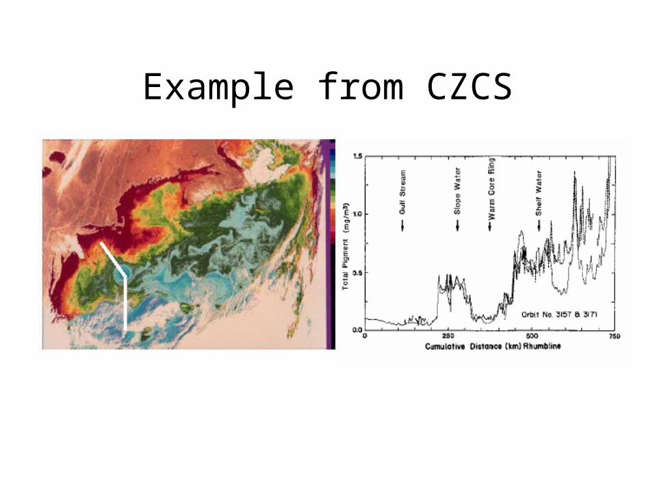
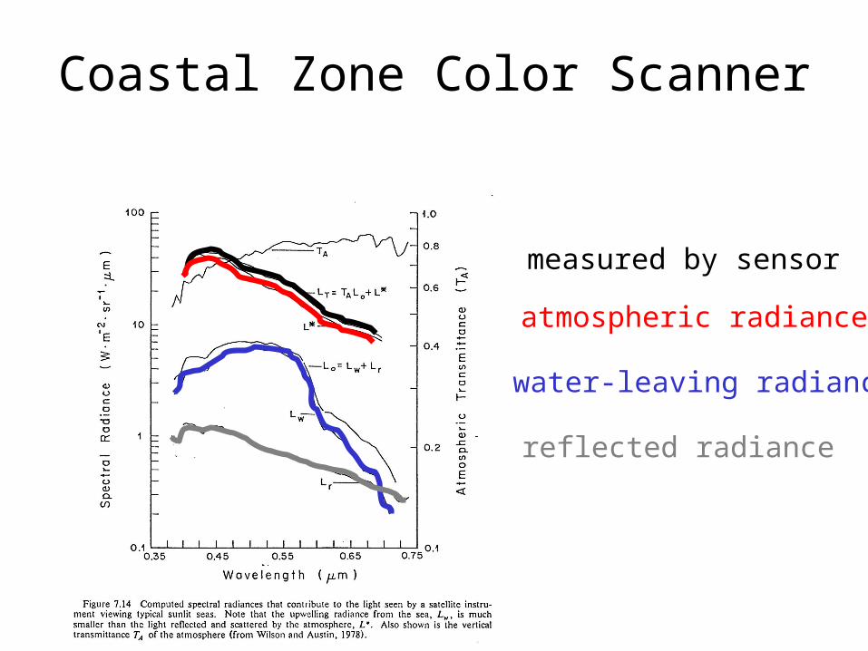
Example from CZCS

Which lead to the first ocean color pigment climatology

Problems with first order algorithm (CZCS)

t*() w() =

t()–r()– (,)(t()- r()–

t*(670)w(670))Check on Assumptions1. w(670) =0 and other assumed clear water values are not valid for even moderate chl~1.0 (no clear water pixel)2. r() is dependent upon surface atm pressure, ozone3. does not really satisfy Angstrom’s Law4. multiple scattering and polarization in the atmosphere are ignored5. t* should be replaced by t and is dependent upon aerosol concentration, particularly absorbing aerosols


Check on Assumptions1. w(670) =0 and other assumed clear water values are not valid for even moderate chl~1.0 (use better in water model but NIR wavelengths would be better)2. r() is dependent upon surface atm pressure, ozone (see corrections by Gregg et al. 2002)3. does not really satisfy Angstrom’s Law (see figures at beginning of lecture, used to define (o) model)4. multiple scattering and polarization in the atmosphere is ignored

Multiple scattering

• error in Rayleigh scattering term approaches – 5% across a scan line– 20% with increasing latitude– greatest for 440 nm, then 670 nm bands

• need to include the Rayleigh-aerosol multiple scattering term


Check on Assumptions1. w(670) =0 and other assumed clear water values are not valid for even moderate chl~1.0 (use better in water model but NIR wavelengths would be better)2. r() is dependent upon surface atm pressure, ozone (see corrections by Gregg et al. 2002)3. does not really satisfy Angstrom’s Law (see figures at beginning of lecture, used to define (o) model)4. multiple scattering and polarization in the atmosphere are ignored (add multiple scattering, polarization terms)5. t* should be replaced by t and is dependent upon aerosol concentration, particularly absorbing aerosols (still ignore assume aerosols are weakly absorbing)

SeaWiFS

Sensor improvements since CZCS

SeaWiFS ~2-4 times more sensitive than CZCSMODIS ~2-4 times more sensitive than SeaWiFSThus we require significantly improved atm correctionto take advantage of added sensitivitye.g. w(443)N < 0.0002

NE – Noise equivalent reflectance

First order correction for SeaWiFS• Still ignore absorbing aerosols

if aerosol is non-abs even up to a=0.2, it works well

when aerosol absorbs, it fails even for low a

First order correction for SeaWiFS• Still ignore absorbing aerosols • use multiple scattering for R/A

• develop look up table for a range of aerosol types• 78 = L(765) ~ La+ra(765), L(865) La+ra(865) select aerosol model AE correction, Km

First order correction for SeaWiFS• Still ignore absorbing aerosols • use multiple scattering for

Rayleigh• use single scattering for aerosol

• use exponential model for ()

(,)

First order correction for SeaWiFS• Still ignore absorbing aerosols • use multiple scattering for

Rayleigh• use single scattering for aerosol

• use exponential model for ()

• use NIR bands 750 and 865 nm for w=0 approximation

water

P.J. Werdell, 2007

Other issues

• “augmented reflectance” of white caps contaminates NIR bands, error improved but still needs work with respect to spectral variations

[wc]N (sr-1)

Moore, Voss, Gordon 2001

Other issues

• Earth’s curvature (Ding and Gordon 1994) still not applied to imagery

• band 7 encompasses an O2 abs band requires correction (Ding and Gordon 1995), corrected in MODIS

• w=0 in NIR

Siegel et al. 2000, relax dark pixel approximation

Use iterative approachchlo w(NIR) atm corr w() and chl1 repeat

Siegel et al. 2000, relax dark pixel approximation

Additional problems in coastal zones

• high CDM concentrations yield low w(blue), and thus requires very high accuracy (issue with negative radiances)

• high sediment loads result in amplified w(NIR) thus impacting aerosol models (see Gordon et al. 2002 site-specific approach for coccolithophore bloom; Ruddick et al. 2000)

• absorbing aerosol (e.g. spectral matching algorithm Gordon et al. 1997 for dust storm events)

Summary from Howard’s to course

can get chl or otherproducts with accuracy approaching surface measurements most of the time

have methods to deal with some episodic events like dust storms

have a reasonable foundation for coastal water algorithms

So say we have the atmospheric correction nailed down and we retrieve water-leaving

radiance, Lw

Variations in the radiance ratios for channels 1 through 3 are interpreted solely as variations in chlorophyll concentration

R13

R12

R23

And the relationship of the radiance ratios to chl…

in log-log spaceover a dynamic rangeof 0.1 to 100 mg/m3

SeaWiFS chl algorithm

• OC4.4

http://seawifs.gsfc.nasa.gov/SEAWIFS/RECAL/Repro3/Figures/oc4_v4_stats_plot_sm.gif

http://seawifs.gsfc.nasa.gov/SEAWIFS/RECAL/Repro3/Figures/oc4_v4_stats_plot_sm.gif

MODIS chl algorithm

• OC3

R = log10 (R443>R490)/R550

a = [2/830,-2.753,1.457,0.659,-1.403]

A note about SeaWiFS and MODIS

• SeaWiFs has a routine calibration cycle that MODIS lacks

• How to account for long term sensor drift– Absolute Calibration– Vicarious Calibration – Use SeaWiFS– Validation

Take Home Messages• It is amazing that we can retrieve robust

estimates of chlorophyll with better than 1 km resolution from over 800 km above the earth and through the atmosphere that contributes 97% of the observed signal

• Remote sensing of ocean color works because…– most of the Lw variability in the blue is related to

phytoplankton biomass (chl)– we do a pretty good job with atmospheric correction

• One irony of ocean color remote sensing is that Rbb/a+bbaphytchl then we use chlIOPs (Hmm)

• We will talk later about reflectance inversions

Formerly Lecture 12 now Lecture 10: Introduction to Remote Sensing and Atmospheric Correction*...

Documents

Transcript of Formerly Lecture 12 now Lecture 10: Introduction to Remote Sensing and Atmospheric Correction*...