
FORests and HYdrology under Climate Change in Switzerland ... · hydrology through its effects on...
28
Geosci. Model Dev., 13, 537–564, 2020 https://doi.org/10.5194/gmd-13-537-2020 © Author(s) 2020. This work is distributed under the Creative Commons Attribution 4.0 License. FORests and HYdrology under Climate Change in Switzerland v1.0: a spatially distributed model combining hydrology and forest dynamics Matthias J. R. Speich 1,2,3,4,5 , Massimiliano Zappa 2 , Marc Scherstjanoi 1,6 , and Heike Lischke 1 1 Dynamic Macroecology, Swiss Federal Research Institute WSL, 8903 Birmensdorf, Switzerland 2 Hydrological Forecasts, Swiss Federal Research Institute WSL, 8903 Birmensdorf, Switzerland 3 Department of Environmental Systems Science, ETH Zurich, 8092 Zurich, Switzerland 4 Biometry and Environmental Systems Analysis, University of Freiburg, 79085 Freiburg im Briesgau, Germany 5 Institute of Sustainable Development, Zurich University of Applied Sciences (ZHAW), 8401 Winterthur, Switzerland 6 Institute of Climate-Smart Agriculture, Johann Heinrich von Thünen Institute, 38116 Braunschweig, Germany Correspondence: Matthias J. R. Speich ([email protected], [email protected]) Received: 29 April 2019 – Discussion started: 2 July 2019 Revised: 30 December 2019 – Accepted: 6 January 2020 – Published: 11 February 2020 Abstract. We present FORHYCS (FORests and HYdrology under Climate Change in Switzerland), a distributed ecohy- drological model to assess the impact of climate change on water resources and forest dynamics. FORHYCS is based on the coupling of the hydrological model PREVAH and the for- est landscape model TreeMig. In a coupled simulation, both original models are executed simultaneously and exchange information through shared variables. The simulated canopy structure is summarized by the leaf area index (LAI), which affects local water balance calculations. On the other hand, an annual drought index is obtained from daily simulated po- tential and actual transpiration. This drought index affects tree growth and mortality, as well as a species-specific tree height limitation. The effective rooting depth is simulated as a function of climate, soil, and simulated above-ground veg- etation structure. Other interface variables include stomatal resistance and leaf phenology. Case study simulations with the model were performed in the Navizence catchment in the Swiss Central Alps, with a sharp elevational gradient and climatic conditions rang- ing from dry inner-alpine to high alpine. In a first experi- ment, the model was run for 500 years with different con- figurations. The results were compared against observations of vegetation properties from national forest inventories, re- motely sensed LAI, and high-resolution canopy height maps from stereo aerial images. Two new metrics are proposed for a quantitative comparison of observed and simulated canopy structure. In a second experiment, the model was run for 130 years under climate change scenarios using both ideal- ized temperature and precipitation change and meteorologi- cal forcing from downscaled GCM-RCM model chains. The first experiment showed that model configuration greatly influences simulated vegetation structure. In particu- lar, simulations where height limitation was dependent on en- vironmental stress showed a much better fit to canopy height observations. Spatial patterns of simulated LAI were more realistic than for uncoupled simulations of the forest land- scape model, although some model deficiencies are still ev- ident. Under idealized climate change scenarios, the effect of the coupling varied regionally, with the greatest effects on simulated streamflow (up to 60 mm yr -1 difference with re- spect to a simulation with static vegetation parameters) seen at the valley bottom and in regions currently above the tree- line. This case study shows the importance of coupling hy- drology and vegetation dynamics to simulate the impact of climate change on ecosystems. Nevertheless, it also high- lights some challenges of ecohydrological modeling, such as the need to realistically simulate the plant response to in- creased CO 2 concentrations and process uncertainty regard- ing future land cover changes. Published by Copernicus Publications on behalf of the European Geosciences Union.
Transcript of FORests and HYdrology under Climate Change in Switzerland ... · hydrology through its effects on...

Geosci Model Dev 13 537ndash564 2020httpsdoiorg105194gmd-13-537-2020copy Author(s) 2020 This work is distributed underthe Creative Commons Attribution 40 License
FORests and HYdrology under Climate Change inSwitzerland v10 a spatially distributed modelcombining hydrology and forest dynamicsMatthias J R Speich12345 Massimiliano Zappa2 Marc Scherstjanoi16 and Heike Lischke1
1Dynamic Macroecology Swiss Federal Research Institute WSL 8903 Birmensdorf Switzerland2Hydrological Forecasts Swiss Federal Research Institute WSL 8903 Birmensdorf Switzerland3Department of Environmental Systems Science ETH Zurich 8092 Zurich Switzerland4Biometry and Environmental Systems Analysis University of Freiburg 79085 Freiburg im Briesgau Germany5Institute of Sustainable Development Zurich University of Applied Sciences (ZHAW) 8401 Winterthur Switzerland6Institute of Climate-Smart Agriculture Johann Heinrich von Thuumlnen Institute 38116 Braunschweig Germany
Correspondence Matthias J R Speich (matthiasspeichwslch speichmatthiasgmailcom)
Received 29 April 2019 ndash Discussion started 2 July 2019Revised 30 December 2019 ndash Accepted 6 January 2020 ndash Published 11 February 2020
Abstract We present FORHYCS (FORests and HYdrologyunder Climate Change in Switzerland) a distributed ecohy-drological model to assess the impact of climate change onwater resources and forest dynamics FORHYCS is based onthe coupling of the hydrological model PREVAH and the for-est landscape model TreeMig In a coupled simulation bothoriginal models are executed simultaneously and exchangeinformation through shared variables The simulated canopystructure is summarized by the leaf area index (LAI) whichaffects local water balance calculations On the other handan annual drought index is obtained from daily simulated po-tential and actual transpiration This drought index affectstree growth and mortality as well as a species-specific treeheight limitation The effective rooting depth is simulated asa function of climate soil and simulated above-ground veg-etation structure Other interface variables include stomatalresistance and leaf phenology
Case study simulations with the model were performed inthe Navizence catchment in the Swiss Central Alps witha sharp elevational gradient and climatic conditions rang-ing from dry inner-alpine to high alpine In a first experi-ment the model was run for 500 years with different con-figurations The results were compared against observationsof vegetation properties from national forest inventories re-motely sensed LAI and high-resolution canopy height mapsfrom stereo aerial images Two new metrics are proposed for
a quantitative comparison of observed and simulated canopystructure In a second experiment the model was run for130 years under climate change scenarios using both ideal-ized temperature and precipitation change and meteorologi-cal forcing from downscaled GCM-RCM model chains
The first experiment showed that model configurationgreatly influences simulated vegetation structure In particu-lar simulations where height limitation was dependent on en-vironmental stress showed a much better fit to canopy heightobservations Spatial patterns of simulated LAI were morerealistic than for uncoupled simulations of the forest land-scape model although some model deficiencies are still ev-ident Under idealized climate change scenarios the effectof the coupling varied regionally with the greatest effects onsimulated streamflow (up to 60 mm yrminus1 difference with re-spect to a simulation with static vegetation parameters) seenat the valley bottom and in regions currently above the tree-line This case study shows the importance of coupling hy-drology and vegetation dynamics to simulate the impact ofclimate change on ecosystems Nevertheless it also high-lights some challenges of ecohydrological modeling suchas the need to realistically simulate the plant response to in-creased CO2 concentrations and process uncertainty regard-ing future land cover changes
Published by Copernicus Publications on behalf of the European Geosciences Union
538 M J R Speich et al FORHYCS a spatially distributed model combining hydrology and forest dynamics
1 Introduction
Of the manifold effects of climate change many are ex-pected to impact the interactions between the water cycleand forest dynamics As a result of higher temperatures andshifts in precipitation regimes an increase in the frequencyand intensity of drought events is predicted (Allen et al2010) as experienced in Europe in 2003 and 2018 Thismay greatly affect tree growth and mortality even in loca-tions currently not subject to high water stress (Choat et al2012 Martin-Benito and Pederson 2015) This affects hy-drologically relevant vegetation properties such as leaf areaindex (LAI) (Tesemma et al 2015) root depth or biomass(Breacuteda et al 2006) and stomatal conductance which varywith stand age or species composition (Ewers et al 2005Ford et al 2011) These changes might affect streamflowand also feed back on local conditions for growth by alteringwater availability For example various studies have shownthat trees growing in thinner stands are subject to lower wa-ter stress so that artificial thinning may mitigate drought ef-fects on tree growth and mortality (Elkin et al 2015) andincrease water yield (McLaughlin et al 2013) Also hydro-logical sensitivity of catchments to climate change seems todepend on vegetation properties with mixed forests show-ing a more stable water yield than catchments dominatedby broadleaf or coniferous forests (Creed et al 2014) Fur-thermore increased atmospheric CO2 is expected to impacthydrology through its effects on stomatal activity and plantproductivity (Trancoso et al 2017) although the long-termeffects are still subject to high uncertainty and debate (Med-lyn et al 2011) Another ecohydrologically relevant compo-nent of global change is land cover change driven not onlyby a change in human land use but also by natural vege-tation dynamics Increases in forested area usually reducestreamflow (Andreacuteassian 2004 Bosch and Hewlett 1982)although the magnitude of such changes varies strongly withcatchment characteristics such as climate soil and forest age(Andreacuteassian 2004) Also catchment response is often non-stationary especially in the case of afforestation or reforesta-tion where streamflow strongly depends on stand age (Farleyet al 2005) Recent model developments have aimed at im-proving predictions by including transient vegetation param-eters to simulate the transition between forest and non-forest(Du et al 2016 Nijzink et al 2016)
Mountainous regions are particularly sensitive to globalchange Among the main effects are the changing signif-icance of seasonal snow storage (Speich et al 2015) al-tered species composition in temperature-limited ecosystems(Mayor et al 2017) and an upwards shift of the treeline(Gehrig-Fasel et al 2007) Given the high significance ofmountains for large-scale water supply (Viviroli et al 2003)it is crucial to estimate how the factors affecting water supplywill change in the future In Switzerland mountains makeup two-thirds of the territory and are of high importance fornature conservation energy production tourism and farm-
ing among other sectors (SCNAT 2012) Modeling studiespredict a change in runoff regime due to increased temper-atures changing precipitation seasonality and glacier melt(Roumlssler et al 2014) with important but locally varying con-sequences for hydropower generation (Gaudard et al 2014)and farming (Milano et al 2015) Climate impacts on forestsalso vary locally with an increase in drought stress pre-dicted at lower elevations and improved growth conditions inenergy-limited high-altitude forests (Bugmann et al 2014)leading to shifting spatial patterns of species compositiontree biomass and canopy cover (Bugmann et al 2014 Fuhreret al 2006) The increased frequency of extreme droughtswill probably be a more important factor than a changein long-term averages (Fuhrer et al 2006) Additionallyabandonment of high-mountain pastures driven by socioe-conomic processes is an important factor of land-use change(Price et al 2016) interacting with climate change to al-low the tree line to shift upwards (Gehrig-Fasel et al 2007)These developments and predictions highlight the need foran integrated simulation of hydrology forest dynamics andland-use change in Switzerland
11 Coupled models of hydrology and forest dynamics
Interactions between hydrology and vegetation dynamics areincluded in various types of dynamic models with widelydifferent areas of application levels of complexity and spa-tial and temporal resolutions (Fatichi et al 2016) One suchdomain is that of land surface models (LSMs) which rep-resent land surface processes in climate models (eg CLMLawrence et al 2011) The main role of vegetation in thesemodels is the partitioning of energy between sensible and la-tent heat fluxes The latter consist of evaporation and tran-spiration thus representing the coupling between the vege-tation hydrology and atmosphere Over time the represen-tation of vegetation and evaporative fluxes in LSMs grewincreasingly complex moving from a simple vegetation-independent bucket model in early applications to a detaileddescription of vegetation processes in particular physiolog-ical processes such as photosynthesis carbon assimilationand nutrient cycling (see review by Seneviratne et al 2010)For a representation of vegetation dynamics climate mod-els are sometimes coupled with dynamic global vegetationmodels (eg LPJ Sitch et al 2003) which can also be usedfor offline simulations Although the primary objective ofthese models is to simulate vegetation patterns they usuallyinclude a representation of terrestrial water balance and areable to simulate river discharge (Gerten et al 2004)
While these models typically operate at the global scaleand for computational efficiency simplify vegetation to a sin-gle average individual per plant type and coarse grid cellsome ecosystem models have been developed to depict veg-etation structure such as the dynamic vegetation model LPJ-GUESS (Smith et al 2001) which is based on individualplants Like LPJ this model contains a soil hydrology mod-
Geosci Model Dev 13 537ndash564 2020 wwwgeosci-model-devnet135372020
M J R Speich et al FORHYCS a spatially distributed model combining hydrology and forest dynamics 539
ule that can be used to calculate discharge but such predic-tions were greatly improved by adding a coupling to a routingscheme (Tang et al 2013) A sensitivity analysis by Pappaset al (2013) pointed out that despite of its detailed mechanis-tic representation of transpirational demand and stomatal clo-sure that affects carbon uptake water stress effects are rep-resented inaccurately in LPJ-GUESS As the various effectsof water shortage on trees are well documented (McDowellet al 2008) this may be seen as a weakness of LPJ-GUESSespecially since important plant functions like cavitation orleaf area reduction under drought conditions are not imple-mented yet (Pappas et al 2013 Manusch et al 2014)
Another type of model representing the interface of hy-drology and vegetation is the forest water balance modelThese models usually simulate the local water balance offorest stands to predict the influence of climatic change orforest management practices on growth conditions for treesExamples include WAWAHAMO (Zierl 2001) or BILJOU(Granier et al 1999) These models may be coupled withdynamic forest models (Lischke and Zierl 2002 Seely et al2015) or run with vegetation parameters assimilated fromforest inventories (Zierl 2001 De Caacuteceres et al 2015) or re-mote sensing (Chakroun et al 2014) Moreover most forestdynamics models include a water balance module (Bugmannand Cramer 1998 Seidl et al 2012) However its role isusually restricted to quantifying soil moisture stress and it isseldom used to predict streamflow
Various hydrological models operating at the catchmentscale have been used to evaluate the effect of land-use changeand the resulting change in vegetation on streamflow Suchmodels include distributed models with a high spatial reso-lution allowing for a detailed mapping of static vegetationparameters eg DHSVM (Wigmosta et al 1994) Othermodels include a simple vegetation growth module such asSWAT (Watson et al 2008) or SWIM (Wattenbach et al2005) More complex models include a detailed representa-tion of average plant biomass growth carbon and nutrient cy-cling and hydrological processes such as RHESSys (Tagueand Band 2004) or Tethys-Chloris (Fatichi et al 2012)
Furthermore the impact of vegetation dynamics onstreamflow has also been studied with models that were notoriginally developed to this effect For example Sutmoumllleret al (2011) used the physically based distributed hydrolog-ical model WaSiM-ETH (Schulla 2015) to perform hydro-logical simulations with vegetation parameters derived froman individual-based forest model driven by different forestmanagement scenarios which influence forest structure andspecies composition Also Schattan et al (2013) applied thesemi-conceptual hydrological model PREVAH (Gurtz et al1999) with vegetation parameters obtained from the forestlandscape model TreeMig (Lischke et al 2006) In the orig-inal versions of both these hydrological models vegetationparameters were parameterized as a function of season andland cover class only This one-way coupling impacted meanannual streamflow by about 10 mm yrminus1 in two large catch-
ments in Switzerland whereas the effect on the local waterbalance reached 40 mm yrminus1 in individual cells Similarly amodeling experiment by Koumlplin et al (2013) showed that in-cluding transient land cover changes such as forest cover in-crease or decrease or glacier retreat could substantially af-fect water balance predictions Such experiments highlightthe importance of considering the dynamics and spatial vari-ability in vegetation properties in hydrological simulations
So far most of the models combining hydrology andvegetation processes have a strong biogeochemical focuswhereas successional dynamics and interspecific competi-tion are rarely considered Couplings between models thatexplicitly simulate forest dynamics and hydrological mod-els have so far mostly been the object of experimental stud-ies The results from these experiments show that couplingthese processes may substantially alter model results and be-havior (Sutmoumlller et al 2011 Schattan et al 2013) Thisgives an opportunity to increase the confidence in simulatedimpacts of climate change on forested ecosystems For reli-able country-level predictions of long-term climate impactson water resources and forest structure and composition in amountainous country such as Switzerland a model should
ndash explicitly simulate the feedbacks between forest prop-erties and hydrology
ndash return estimates of streamflow and (evapo)transpirationas well as tree species distribution and biomass
ndash operate at a spatial resolution fine enough to accountfor the great variability in climate topography and landcover
ndash be able to simulate the hydrology of non-vegetated areassuch as glaciers bare rock or built-up
ndash take into account the possibility of forest expansion andretreat and
ndash not be too complex so that it can be run for large areasand long periods at a reasonable computational cost
None of the models discussed above fulfill all of thesecriteria This motivated the development of a spatially dis-tributed model combining hydrology and forest dynamicspresented below
12 Aims of this work
In this paper we present a newly developed distributed eco-hydrological model FORHYCS (FORests and HYdrologyunder Climate change in Switzerland) This model com-bines two existing models the hydrological model PREVAH(Gurtz et al 1999) and the forest landscape model TreeMig(Lischke et al 2006) FORHYCS is spatially distributedand operates on a grid of regular cells The model outputsare hydrological quantities such as catchment-integrated
wwwgeosci-model-devnet135372020 Geosci Model Dev 13 537ndash564 2020
540 M J R Speich et al FORHYCS a spatially distributed model combining hydrology and forest dynamics
streamflow and maps of runoff transpiration evaporation orsnow cover and maps of forest properties such as biomassleaf area index (LAI) species distribution and tree densityIn FORHYCS the two source models are run simultane-ously and exchange information through shared variablesFORHYCS may be run in uncoupled mode (ie parallelsimulations of hydrology and forest dynamics without anytransfer of information between the two source models) witha one-way coupling (transfer of information from the forestlandscape model to the hydrological model or vice versa) orin fully coupled mode
Like its parent models FORHYCS may be described assemi-conceptual Hydrological processes (evaporation tran-spiration soil moisture dynamics and runoff generation) andforest dynamics (growth mortality establishment and mi-gration of tree species) are based on physical and ecologicaltheory as well as empirical approaches Thus the degree ofcomplexity of FORHYCS is lower than other coupled eco-hydrological models such as RHESSys (Tague and Band2004) Also unlike these models the focus of the ecologicalpart is on forest dynamics similar to the addition to SWIMproposed by (Wattenbach et al 2005) However FORHYCSdiffers from the latter approach in that growth and mortal-ity are simulated at the level of species and size classes in-stead of a single biomass pool per cell Both TreeMig andPREVAH were designed for applications at an intermediatespatial resolution with a cell size between 100 m and 1 km
The goal of this paper is to explore the interplay of hydrol-ogy and forest dynamics in a coupled model The questionsto be answered are (1) ldquoHow does the coupling impact the be-havior and the performance of both TreeMig and PREVAHcompared to uncoupled simulationsrdquo (2) ldquoWhich aspects ofthe forestndashhydrology coupling are of greatest importance forsimulation resultsrdquo and (3) ldquoWhat are the implications ofmodel coupling for simulations under climate changerdquo
The model is tested in five subcatchments of the Navizencecatchment (27 to 87 km2) located in the Swiss Central AlpsTo answer the first question a full forest succession is mod-eled for the period 1500ndash2015 starting from bare soil Theforest model is run in uncoupled mode to serve as a referencesimulation For the coupled runs various configurations aretested with different aspects of the coupling between hydrol-ogy and forest dynamics switched on and off The outputsare then compared to forest inventory data as well as griddeddatasets of leaf area index (LAI) and canopy height To assessthe effect of the coupling on hydrological predictions sim-ulated streamflow from coupled and uncoupled model runsis compared against a time series of daily measurementsFurthermore to assess the behavior of the coupled and un-coupled model under climate change the model is run fora century under artificial climate change scenarios In thesefuture model runs the significance of two further aspects ofthe forestndashhydrology coupling are examined including theeffect of elevated CO2 on stomatal resistance and the poten-
tial forest expansion into high-elevation meadows as a resultof climate and land-use change
2 Methods and data
21 FORHYCS model description
The two original models operate at a different temporal res-olution while TreeMig simulates forest dynamics with anannual time step PREVAH calculates daily values with aninternal time step of 1 h Both original models are run si-multaneously over the same domain and exchange informa-tion through shared variables Figure 1a shows the flow ofa simulation hydrology is simulated on a daily basis withvegetation properties given by the forest model for the previ-ous year This is based on the assumption that effects of thecurrent-year water balance on the forest structure and com-position are negligible An annual drought index (DI) influ-encing tree growth and mortality (Sect 213) is calculatedin each cell from the transpiration simulated in the hydro-logical model over the whole simulation year (Sect 214)Based on the number of trees per species and height class ineach cell annual maximal values of leaf area index (LAI) andfractional canopy cover (FCC) are calculated These valuesare converted to daily values using a temperature-dependentphenology module (Sect 212) The rooting zone water stor-age capacity (SFC) is updated annually as a function of long-term climate (Sect 215) Furthermore the model includesthe effects of snow-induced mortality for some species usingan additional mortality function based on snow cover dura-tion (Sect 216)
211 Source models
The semi-conceptual hydrological model PREVAH (Gurtzet al 1999) in its fully distributed form (Schattan et al2013 Speich et al 2015) solves the water balance of eachgrid cell by calculating evapotranspiration soil water bal-ance and runoff generation at a sub-daily time step Thecore of PREVAH is based on the structure of the widelyused model HBV (Bergstroumlm 1992) combined with a con-ceptual runoff routing scheme (Gurtz et al 1999) Succes-sive model developments enabled or improved the treatmentof interception (Menzel 1996) snowpack dynamics (Zappaet al 2003) glacier runoff (Klok et al 2001) and ground-water runoff (Gurtz et al 2003) PREVAH was used amongother applications to estimate the impact of climate changeon discharge (Zappa and Kan 2007) Climate impact studieswere also conducted using the distributed outputs of PRE-VAH (Speich et al 2015)
The spatially explicit forest landscape model TreeMig(Lischke et al 2006) simulates forest establishment growthand mortality as well as seed dispersal Originally based ona gap model (Lischke et al 1998) TreeMig calculates thenumber of trees per species and height in each cell and op-
Geosci Model Dev 13 537ndash564 2020 wwwgeosci-model-devnet135372020
M J R Speich et al FORHYCS a spatially distributed model combining hydrology and forest dynamics 541
Figure 1 (a) Flow of a FORHYCS simulation starting in the example year 1971 The initial state can be loaded from a file or a spin-upcan be performed The hydrological calculations are performed daily At the end of the simulation year bioclimatic indices are calculatedand passed to TreeMig which simulates forest dynamics with an annual time step Long-term climate statistics are updated at the end ofthe year based on the daily calculations and the effective rooting depth module is run with the updated climate indices The forest modelreturns an annual maximal LAI value To be used in hydrological calculations this value is converted to daily values based on simulatedleaf phenology Another important interface variable is the rooting zone storage capacity SFC (b) Schematic overview of the couplingsbetween climate above-ground forest structure and the rooting zone in TreeMig (left) and FORHYCS (right) TreeMigrsquos forest structure(speciesndashsize distribution) depends on its previous state and is influenced by the annual bioclimatic indices Unlike the other indices whichdepend on meteorological input only the drought index (DI) further depends on a constant soil moisture storage capacity (ldquobucket sizerdquo) InFORHYCS the drought index further depends on canopy structure through its influence on potential transpiration (PT) Additional optionalcouplings in FORHYCS are the dynamic simulation of a climate-dependent storage capacity of the rooting zone (through varying effectiverooting depth) a limitation of maximum tree height under dry conditions and a drought-dependent reduction of leaf area
erates at an annual time step Inter- and intraspecific com-petition is represented through light distribution within thecanopy which depends on the distribution of trees of dif-ferent heights within a stand and thus on leaf area (Lis-chke et al 1998) TreeMig was used to predict climate im-pact on tree species distribution in Switzerland (Bugmannet al 2014) as well as to simulate forest response to landabandonment (Rickebusch et al 2007) and the feedbacksbetween forests and avalanches (Zurbriggen et al 2014)Abiotic drivers of forest dynamics are represented by threebioclimatic indices mean temperature of the coldest monthdegree-day sum and drought (see Sect 213 for the latter)
212 Canopy structure and leaf phenology
Leaf area index (LAI) is calculated in TreeMig to accountfor mutual shading and competition for light (Lischke et al
1998) In FORHYCS LAI is passed to the hydrologicalmodel replacing the land-cover-specific parameterization inPREVAH The allometric equations of Bugmann (1994) re-late leaf area to diameter at breast height (D in centimeters)As D is allometrically linked to tree height leaf area is cal-culated for each group of trees of the same species and heightclass then summed to obtain the value for the whole stand asfollows
Al =
nspcsumsp=1
nhclsumhc=1
SLAsptimes a1sptimesDa2spsphc timespdsp (1)
where Al is the total all-sided stand leaf area (in square me-ters) nspc is the number of species (30 in FORHYCS) nhclis the number of height classes (16) SLAsp is the specific leafarea (in square meters per kilogram) a1sp (in kilograms percentimeter) and a2sp (unitless) are species-specific allomet-
wwwgeosci-model-devnet135372020 Geosci Model Dev 13 537ndash564 2020
542 M J R Speich et al FORHYCS a spatially distributed model combining hydrology and forest dynamics
ric parameters (Bugmann 1994) and pdsp is a dimension-less reduction term accounting for seasonal variations in leafarea ranging from 0 to 1 (see below and in the Supplement)The reference area in TreeMig is the size of a forest plot setto 833 m2 (112 ha) which is the reference area in many gapmodels (eg Bugmann 1994) so that
LAI= Alkc833 (2)
where kc is a factor to convert from true to projected leafarea set to 05 for broadleaves and 04 for conifers follow-ing Hammel and Kennel (2001) Fractional canopy cover fcis also calculated from the number of trees per species andheight class using the equation of Zurbriggen et al (2014)as follows
fc =1minus exp
minus1timesnspcsumsp=1
nhclsumhc=1
(nsphc833)timesCAsphc
(3)
where CAsphc is the total crown area for trees of each speciesand height class
CAsphc =(ka1sptimesh
2hc+ ka2sptimeshhc
)times nsphc (4)
where ka1sp and ka2sp are species-specific allometric pa-rameters and hhc is the (upper) height of the height class(hc) Minimum values for LAI and fc are set to 02 and 01respectively to account for a minimal cover by grass andshrubs as well as bare stems Annual maximum LAI maybe reduced as a function of the drought stress of the previousyears as described below in Sect 213 It is worth notingthat leaf area and crown area are calculated independentlyfrom each other both using empirical relationships with treesize
To obtain daily values for LAI and fc a leaf phenologymodule has been implemented The variable pdsp reflectsthe phenological status of species ldquosprdquo in a given cell andvaries between 0 (no leaves) and 1 (full foliage) This mod-ule also defines the start and end of the growing season ineach cell which is required to calculate the climatic indicesfor the rooting depth module (Sect 215) In each cell thegrowing season lasts as long as pdsp is greater than 05 forthe dominant species Daily values of pdsp are simulated inspring with the model of Murray et al (1989) which de-pends on the number of chill days in winter and accumu-lated growing degree days in summer When pdsp reachesa value of 1 the foliage is assumed to be fully developedThe onset of leaf senescence in autumn is simulated usingthe model of Delpierre et al (2009) which depends on tem-perature and photoperiod For broadleaves the end of thegrowing season is set to 14 d after the onset of senescenceand pdsp is linearly reduced from 1 to 0 during this periodAlthough the leaf area is not varied throughout the year forevergreen conifers pdsp is still simulated to define the start
and end of the growing season For these species (as well asfor the deciduous conifer Larix decidua) the developmentof pdsp following the onset of senescence is calculated us-ing the formulation of Scherstjanoi et al (2014) The param-eters for the empirical models of Murray et al (1989) andDelpierre et al (2009) were calibrated against phenologicalobservations across Switzerland (Defila and Clot 2001) Thespecies-specific parameters and a description of the calibra-tion procedure are given in the Supplement
213 Drought and its effects on forest growthmortality and structure
The drought index used in TreeMig is based on the ratioof annual to potential evapotranspiration as calculated witha module modified from Thornthwaite and Mather (1957)This scheme requires a monthly precipitation sum and tem-perature average for each cell as well as the plant-availablewater storage capacity Evaporative demand is calculatedusing an empirical temperature-dependent approach andmonthly soil water balance is simulated based on watersupply and demand after accounting for interception (seeBugmann and Cramer 1998 for a full description of thisscheme) This approach has a number of drawbacks Firstit does not consider the effect of variations in vegetationproperties on evaporative supply and demand thus neglect-ing feedbacks between vegetation density transpiration anddrought (see eg Kergoat 1998) Also the ThornthwaitendashMather routine does not account for snow-related processeswhich can lead to large errors in the estimation of evapo-transpiration diminishing the representativeness of the in-dex for growth conditions (Anderegg et al 2013) Further-more empirical evapotranspiration formulations such as theThornthwaitendashMather routine rely to a large extent on cali-brated values These may not be transferrable to climatic con-ditions that differ from the calibration period (Bartholomeuset al 2015) limiting the ability of the model to make predic-tions under a changing climate For these reasons this abioticdrought index was replaced by a relative transpiration index(Speich et al 2018a) This index is similar to the evapotran-spiration deficit index presented above but is based on tran-spiration rather than evapotranspiration as follows
DI= 1minussumds
d=deET actdsumdsd=deET potd
(5)
where de and ds are the first and last day of the periodfor which the drought stress is calculated and ET potd andET actd are modeled daily canopy transpiration sums (in mil-limeters per day) Here DI is calculated for the entire yearso that de= 1 and ds= 365 Furthermore to account for de-layed effects of drought on tree physiology (Hammel andKennel 2001) the average of the last 3 years is used hereTranspiration is reduced from the potential rate through theeffect of low soil moisture or high atmospheric vapor pres-sure deficit (VPD) on stomatal resistance (Eq 14 in Speich
Geosci Model Dev 13 537ndash564 2020 wwwgeosci-model-devnet135372020
M J R Speich et al FORHYCS a spatially distributed model combining hydrology and forest dynamics 543
et al 2018a) The rationale behind this index is based onthe fact that stomatal closure is one of the first responses of aplant to water deficit Therefore the time during which stom-atal resistance is increased due to drought is the time duringwhich adverse physiological effects of water shortage (egcavitation reduced carbon uptake) are likely to occur andDI serves as a proxy for all these processes The effect ofVPD was included to account for the effects of high evapo-rative demand on plant-internal hydraulics (Zierl 2001) Thedrought stress function fDS determines the relative drought-induced limitation of annual growth (Bugmann 1994)
fDS =
radicmax
(01minus
DIkDT
) (6)
where kDT is a species-specific drought tolerance parame-ter indicating the value of DI at which growth is completelysuppressed This growth reduction function can take valuesbetween 0 (complete growth suppression) and 1 (unstressedconditions) Annual growth of the trees of the same speciesand height class is the product of a species-specific maxi-mal growth an environmental reduction function fenv and afurther reduction term accounting for shading The environ-mental reduction function is the geometric mean of fDS andtwo other stress functions representing the effects of temper-ature and nitrogen availability (Bugmann 1994) While theeffects of temperature are taken into account in this study ni-trogen availability is kept spatially and temporally constantThese two environment-dependent stress functions are fur-ther described in Sect S12 of the Supplement (for a descrip-tion of the effects of light competition and shading we re-fer to (Lischke et al 2006) The same reduction function isused to simulate mortality in addition to background mor-tality and applies if it is more severe than mortality causedby low productivity Lischke and Zierl (2002) parameterizedkDT for the 30 tree species represented in TreeMig by over-laying modeled DI with inventory-derived maps of speciesdistribution The values range between 027 and 05 How-ever this parameterization did not lead to satisfactory simu-lations of species composition in the case study of this paperTherefore species-specific kDT was defined based on a com-bination of the rankings by Lischke and Zierl (2002) and Ni-inemets and Valladares (2006) Table S7 in the Supplementlists the kDT values used in this study
FORHYCS accounts for two additional effects of droughtstress a limitation of maximum height and a reduction ofannual maximal LAI The former is parameterized follow-ing Rasche et al (2012) ie species-specific maximum treeheight may be reduced as a function of the bioclimatic in-dices DI and DDEGS (degree-day sum see Sect S12 of theSupplement) The parameter kredmax which is also species-specific indicates the fraction of maximum height that canbe attained by trees if one of the environmental vitality func-tions is at its minimum The more severe of the two reduc-tions (drought or degree-days) is applied Unlike in the for-
mulation of Rasche et al (2012) where the reduction is alinear function of the bioclimatic indices the impact func-tions (Eq 6 for drought and S8 for degree-day sum) are usedhere
The LAI reduction function follows the formulation ofLandsberg and Waring (1997) where the fraction of carbonallocated to roots increases under stress whereas allocationto foliage and stem decreases Since allocation is not ex-plicitly simulated in FORHYCS the following formulationis purely phenomenological For all size classes of a givenspecies leaf area is scaled by the ratio of the foliage allo-cation coefficient under current ηl and unstressed conditionsηlu Eq (1) is thus modified as follows
Al =
nspcsumsp=1
nhclsumhc=1
SLAsptimes a1sptimesDa2spsphc timespdsp
times ηlspηlusp (7)
The allocation coefficients for foliage are calculated as fol-lows
ηl = 1minus ηrminus ηs and ηlu = 1minus ηruminus ηsu (8)
where ηr and ηru are the allocation coefficients to roots andηs and ηsu are the allocation coefficients to the stem un-der current and unstressed conditions respectively Follow-ing Landsberg and Waring (1997) ηru is set to 0229 and ηrincreases with increasing stress by the following relation
ηr =08
1+ 25(1minus fenv) (9)
where fenv is the geometrical mean of the drought and lowtemperature stress functions (Eqs 6 and S8) The carbon al-located to the stem is related to ηr as follows
ηs = (1minus ηr)(pls+ 1
) and
ηsu =(1minus ηru
)(pls+ 1
) (10)
where pls is the ratio of the growth rates of leaves and stemsin terms of their change in relation to diameter at breastheight D In FORHYCS pls is calculated using the allo-metric equations used to calculate leaf and stem biomass
pls =dwldDdwsdD
=kl1D
kl2
ks1Dks2 (11)
where kl1 and kl2 are allometric parameters for leaf biomassand ks1 and ks2 are allometric parameters for stem biomass(Bugmann 1994) It is important to stress that FORHYCSdoes not explicitly simulate carbon assimilation HenceEqs (9) and (10) are only used to determine a reduction fac-tor for leaf area (Eq 8) and have no direct influence on sim-ulated tree growth stem biomass and rooting depth
wwwgeosci-model-devnet135372020 Geosci Model Dev 13 537ndash564 2020
544 M J R Speich et al FORHYCS a spatially distributed model combining hydrology and forest dynamics
214 Partitioning of transpiration and soil evaporation
The implementation of the new drought index (see Sect 213above) required some changes to the evapotranspiration rou-tine in the hydrological model While the relative transpi-ration index is based on estimates of actual and potentialtranspiration PREVAH does not explicitly differentiate be-tween transpiration and soil evaporation Therefore a newlocal water balance routine was implemented based on thestandalone model FORHYTM (Speich et al 2018a) Thismodule combines the soil water balance formulation of theHBV model (Bergstroumlm 1992) which is also implementedin PREVAH with the transpiration and evaporation schemeof Guan and Wilson (2009) and a Jarvis-type (Jarvis 1976)parameterization of canopy resistance A full description isgiven in Speich et al (2018a)
The parameterization of canopy resistance differs from theoriginal formulation in two ways First the effect of atmo-spheric vapor pressure deficit (VPD) on stomatal conduc-tance is represented with a negative exponential function in-stead of a linear function Second an additional canopy re-sistance modifier (f5) was implemented to account for theeffect of atmospheric CO2 concentration (Ca [micromol molminus1])This function is based on the results of Medlyn et al (2001)
f5 =
(1minus jc
(min(Ca700)
350minus 1
))minus1
(12)
where jc represents the fractional change in conductance inresponse to an increase in Ca from 350 to 700 micromol molminus1
and was set to 01 for coniferous forests 025 for broadleafforests and 018 for mixed forests (the forest type in each cellis determined based on the relative share of above-groundbiomass belonging to conifers and broadleaves) These val-ues were set based on the results reported by Medlyn et al(2001) coniferous species had a value of jc between 0 and02 whereas broadleaves had values up to 04 Thereforefor conifers a value of 01 was selected For broadleavesas there seemed to be some acclimation for trees growingin elevated CO2 a more conservative (than 04) value of025 was chosen The value for mixed forests correspondsto the arithmetic mean of the two This affects both po-tential and actual transpiration so that with all other fac-tors kept constant increases in Ca will reduce the level ofdrought stress The rationale for implementing this new wa-ter balance scheme is to account for the effect of variationsin vegetation properties (eg LAI) on physiological droughtin forests As FORHYCS includes the possibility of chang-ing land cover classes in a cell some non-forested cells maybecome forested over the course of a simulation As vege-tation parameters (such as LAI and effective rooting depth)are prescribed as a function of land cover for non-forestedcells this shift inevitably introduces an artificial discontinu-ity in the simulation To reduce this discontinuity the newwater balance scheme is also used for potentially forestedland cover types On the other hand for land cover types that
cannot become forested the original water balance schemeof PREVAH (Gurtz et al 1999) is applied
215 Rooting zone storage capacity
The rooting zone water holding capacity SFC is calculatedas the product of effective root depth Ze and soil water hold-ing capacity κ (Federer et al 2003) While κ is assumedto remain constant Ze is assumed to vary as a function ofvegetation characteristics and climate The approach usedto parameterize Ze is the carbon costndashbenefit approach ofGuswa (2008 2010) This approach rests on the assump-tion that plants dimension their rooting systems in a waythat optimizes their carbon budget The optimal rooting depthis the depth at which the marginal carbon costs of deeperroots (linked to root respiration and construction) starts tooutweigh the marginal benefits (ie additional carbon up-take due to greater availability of water for transpiration)The implementation of this model in FORHYCS follows theprocedure described by Speich et al (2018b) Effective root-ing depth expressed as an average over the whole cell iscalculated for both overstory (trees) and understory (shrubsand non-woody plants) The storage volume SFC for a givencell is defined as the sum of these two area-averaged rootingdepths multiplied with soil water holding capacity κ A fulldescription of this implementation is given in Speich et al(2018b) The underlying equation is
γrtimesDr
Lr= wphtimes fseastimes
d〈T 〉dZe
(13)
where γr is root respiration rate (in milligrams of carbon pergram of roots per day) Dr is the root length density (in cen-timeters of roots per cubic centimeter of soil) Lr is the spe-cific root length (in centimeters of roots per gram of roots)wph is the photosynthetic water use efficiency (in grams ofcarbon per cubic centimeter of H2O) fseas is the growingseason length (fraction of a year) and 〈T 〉 is the mean dailytranspiration (in millimeters per day) during the growing sea-son The left hand side represents the marginal cost of deeperroots and the right hand side the marginal benefits solvingfor Ze gives the optimal rooting depth Any equation can beused to relate d〈T 〉 to dZe In this implementation the prob-abilistic models of Milly (1993) and Porporato et al (2004)are used for the understory and overstory respectively Thesetwo models reflect the differing water uptake strategies ofgrasses and trees (Guswa 2010) Both models estimate tran-spiration based on soil water holding capacity κ and long-term averages of climatic indices Evaporative demand is rep-resented by potential transpiration and rainfall is representedas a marked Poisson process characterized by the frequency(λ in events per day) and mean intensity (α in millimetersper event) of events In FORHYCS these variables are cal-culated as rolling means with a window of 30 years includ-ing only the growing seasons Potential transpiration for theunderstory and overstory are taken from the calculations of
Geosci Model Dev 13 537ndash564 2020 wwwgeosci-model-devnet135372020
M J R Speich et al FORHYCS a spatially distributed model combining hydrology and forest dynamics 545
the local water balance module (Sect 214) and the rainfallcharacteristics are taken from modeled effective precipitation(ie after accounting for interception) The start and end ofthe growing season are determined based on the phenologymodule (Sect 212) In addition mean daily air temperatureis calculated over the growing season to adjust respirationrate The plant-specific parameters in Eq 13 are summarizedin the variable PPo defined as follows
PPo =γr20Dr
Lrwph (14)
where γr20 is the root respiration rate at 20 C The ac-tual root respiration rate is dependent on annually averagedtemperature via a Q10 function For further details pleaserefer to Speich et al (2018b) A higher value of PPo in-dicates a greater difficulty for the plant to develop addi-tional roots In FORHYCS PPo was set to 1263times 10minus4 forconifers and 101times10minus4 for broadleaved species At the celllevel PPo was averaged based on the relative share of above-ground biomass belonging to conifers and broadleaves Forthe understory the corresponding parameter PPu is set to1512times 10minus4
216 Snow-cover induced seedling mortality
For seedlings of the high-mountain species Larix deciduaPinus cembra and P montana the model also includes theeffect of snow-induced fungal infections via the variableFDSA (final day of snow ablation) as described by Zur-briggen et al (2014) An additional mortality term is calcu-lated as follows
micros = atimesFDSA2+ btimesFDSA+ c (15)
where a b and c are empirical parameters fitted by Zur-briggen et al (2014) for Larix decidua and for the twoaforementioned Pinus species If micros is greater than back-ground mortality or the mortality term integrating lighttemperature and water stress it is applied instead for theseedlings of these species This aspect of the model was im-plemented to examine the feedback between forest dynamicsand avalanches on a small spatial scale (Zurbriggen et al2014) but was never tested on landscape scale Here FDSAis defined as the last day of the year with more than 5 mm ofsnow water equivalent
217 Uncoupled mode and one-way coupling
The methods have so far described the model FORHYCS inits fully coupled version It is also possible to run FORHYCSin uncoupled mode (without any information transfer be-tween the hydrological and forest models) or with a one-way coupling (information transfer from the forest modelto the hydrological model only) An uncoupled FORHYCSrun consists essentially of a PREVAH run and a TreeMigrun happening independently from each other Uncoupled
FORHYCS differs from other PREVAH implementationsmainly through the parameterization of soil and surfaceproperties As mentioned in Sect 42 previous applicationsof PREVAH in Switzerland have used soil depth and wa-ter holding capacity from the agricultural suitability mapBEK (BfR 1980) Preliminary analyses in this project haveshown that this parameterization gave implausible resultswhen used with the newly implemented water balance mod-ule (Sect 214) Therefore to ensure comparability betweencoupled and uncoupled runs all FORHYCS runs use the soilparameterization from Remund and Augustin (2015) (seeSect 222) in forested cells In uncoupled runs it is assumedthat the rooting depth of forests is 1 m As this dataset wasdeveloped based on forest soil profiles values for cells out-side currently forested areas are not reliable (Jan RemundMeteotest personal communication 2015) To simulate for-est expansion under climate and land-use change scenariosit was nevertheless assumed that cell values of the RA2015(Remund and Augustin 2015) dataset represent the waterstorage capacity for 1 m of soil depth To account for shal-lower rooting of non-forest vegetation types a land-cover-dependent rooting depth parameter was introduced The pa-rameter values for different land cover types are given inTable S6 Non-vegetated land cover classes (eg built-upor bare rocks) use the same standard soil parameters as inthe original PREVAH (Gurtz et al 1999) Another differ-ence between FORHYCS and PREVAH is the parameteriza-tion of canopy resistance Whereas PREVAH gives a mini-mum canopy resistance for each land cover class (ie nor-malized by leaf area index) the new water balance mod-ule requires a minimum stomatal resistance Following Guanand Wilson (2009) minimum stomatal resistance was setto 180 s mminus1 for forests 130 s mminus1 for meadows and grass-lands and 210 mminus1 for shrubs
One-way coupling is similar to the modeling experimentof Schattan et al (2013) vegetation variables from TreeMigare passed to PREVAH but there is no feedback from thehydrological to the forest model This configuration uses theabiotic drought index calculated with FORCLIM-E (Bug-mann and Cramer 1998) In this study TreeMig was runwith two soil datasets (BEK and RA2015 see below) In allcases the hydrological part of the model uses the RA2015dataset In this study rooting zone storage capacity SFCof the hydrological model was kept constant in one-waycoupled mode assuming a rooting depth of 1 m Enablingclimate-dependent adaptation of SFC in this mode would im-pact simulation results for the hydrology part but not for theforest
22 The Navizence case study
221 Catchment description
The Navizence catchment is located in the Swiss CentralAlps and covers an area of 255 km2 To enable the future mi-
wwwgeosci-model-devnet135372020 Geosci Model Dev 13 537ndash564 2020
546 M J R Speich et al FORHYCS a spatially distributed model combining hydrology and forest dynamics
gration of tree species that are currently not represented in thecatchment the modeling area extends beyond the catchmentto form the rectangular area shown in Fig 2 (1079 km2)The catchment is characterized by a sharp elevational gradi-ent with elevations ranging from 522 to 4505 m asl Likein its neighboring valleys this gradient is reflected in thehydro-climatic conditions Due to the shielding effect ofmountain ranges the Rhocircne valley where the catchmentoutlet is located is the driest region of Switzerland withthe mean annual precipitation (MAP 1981ndash2010) at Siontotaling 603 mm (MeteoSwiss 2014) However the valleypresents a strong altitudinal precipitation gradient with MAPexceeding 2500 mm at 3000 m asl most of it falling assnow (Reynard et al 2014)
Tree species composition shows a rather clear altitudinalzonation with drought-resistant species (Pinus sylvestris andQuercus spp) dominating at lower elevations whereas Piceaabies Larix decidua and Abies alba dominate the subalpinestage and the treeline is formed by Larix decidua and Pinuscembra The landscape is heavily influenced by human ac-tivity with a large fraction of land occupied by settlementscropland vineyards and pastures Furthermore nearly allforests in the area are subject to management in variousforms and degrees of intensity with a considerable impacton forest dynamics Specifically many forests were clear-cut between the Middle Ages and the nineteenth centurymostly for fuel (Burga 1988) In the first half of the twenti-eth century the quantitatively most important anthropogenicdisturbance factors were litter collecting and wood pasture bygoats (Gimmi et al 2008) Nowadays these practices havebeen largely abandoned and timber harvesting plays a lim-ited role in the region As a result of past and current an-thropogenic factors the main deviations from potential natu-ral forest composition are (1) silvicultural practices favoringcertain species such as Pinus sylvestris and Larix decidua(2) effects of litter removal and grazing and (3) a replace-ment of L decidua and Pinus cembra by mountain pastures(Buumlntgen et al 2006) and dwarf shrubs (Burga 1988) nearthe treeline
Currently three major hydropower plants are operationalin the valley with a total installed capacity of 164 MW anda mean net annual production of 570 GWh The main reser-voir is the artificial lake Lac de Moiry located in a lateralvalley with a storage capacity of 77 million m3 A system ofpipelines has been built to divert water from the Navizenceas well as from a neighboring catchment into the lake
222 Input data
Three kinds of spatial data are needed to run the model dailymeteorological data time-invariant physiographic data andspatially distributed model parameters for PREVAH Theseparameters represent environmental factors not related tovegetation such as snow glacier and runoff generation pro-cesses Further information on the parameterization of PRE-
VAH is given in Sect S17 of the Supplement The model isdriven by daily values for precipitation (in millimeters) airtemperature (in degrees Celsius) global radiation (in wattsper square meter) wind speed (in meters per second) rela-tive air humidity (percent) and sunshine duration SSD (inhours) provided by the Swiss Meteorological Office Me-teoSwiss (Begert et al 2005)
Physiographic data consists of information on soil to-pography and land cover Soil is represented in terms ofwater holding capacity κ (in millimeters of water depthper millimeter of soil depth) and soil depth Two differentdatasets are used for soil properties In previous applicationsin Switzerland both PREVAH and TreeMig used grids ofκ and soil depth from a countrywide agricultural suitabilitymap (BfR 1980 hereafter referred to as ldquoBEKrdquo) The result-ing rooting zone storage capacities (SFC in millimeters) inthe forested cells of the study region range between 375 and110 mm As this dataset was not specifically developed foruse in forests and some values are implausibly low Remundand Augustin (2015) generated a new countrywide dataset(RA2015) of rooting zone storage capacity on the basis 1234forest soil profiles throughout Switzerland combined with alithological map This dataset gives the volume of water thatcan be stored in the soil for a depth of up to 1 m with lowervalues in cells where soil is assumed to be shallower SFC inthe new dataset ranges from 71 to 223 mm in forested cellsof the study region Figure S1 shows the rooting zone storagecapacity in forested cells of the study region for both soil pa-rameterizations For coupled simulations only the RA2015parameterization is used To facilitate a comparison with re-sults from previous studies the parent models PREVAH andTreeMig are also run with the BEK parameterization
223 Comparison data and metrics of agreement
This section describes the data against which model outputswere compared including three datasets of vegetation prop-erties and one dataset of streamflow measurements Thesedatasets are used to plausibilize model outputs and serve as abasis for the choice of model configuration Daily streamflowwas obtained from the operator of the power plants Thesedata include an accounting of the amount of water divertedthrough the different pipelines From this time series of nat-ural streamflow were reconstructed which were used as ob-servations Further details on the streamflow data are givenin Sect S19 of the Supplement
The simulated stem numbers and above-ground biomasswere compared against data from the first Swiss NationalForest Inventory(NFI Bachofen et al 1988) As the sam-pling plots of the NFI are distributed on a regular grid eachplot is randomly selected from all forest plots in that regionand may not be considered representative for a larger area Itis therefore not sensible to compare simulated and observedbiomass at the scale of single inventory plots Instead the 245NFI plots in the study area were aggregated to seven classes
Geosci Model Dev 13 537ndash564 2020 wwwgeosci-model-devnet135372020
M J R Speich et al FORHYCS a spatially distributed model combining hydrology and forest dynamics 547
Figure 2 Map of the study area including the Navizence catchment and the subcatchments used in this study Streamflow measurementsare available for the subcatchments 2 through 5 As the lowest part of the Navizence catchment (subcatchment 1) differs greatly from theothers in terms of elevation and current land cover modeled streamflow is also examined for this subcatchment although no measurementsare available Forest-related model outputs are evaluated over the entire currently forested area inside and outside the catchment Streamsare drawn for reference only
based on aspect and elevation with four elevation bands fornorth-facing plots and three for south-facing plots This wayeach class has a sample size of at least 30 plots which en-sures that the averages are representative For comparisonwith inventory data simulated biomass was also averagedover the same strata
Simulated LAI was compared to the remotely sensed LAIdataset provided by Copernicus at 300 m resolution (Coper-nicus Service Information 2017) This dataset uses mea-surements of the satellite Proba-V and its temporal cover-age starts in January 2014 The LAI 300 m rasters were re-sampled to match the resolution and extent of the model in-put and output then stratified as described above For eachcell of the original LAI 300 m grids the maximum valueof the 10 d periods contained between May and July of theyears 2014 through 2016 was used as an estimate of maxi-mum LAI independent of intra-annual fluctuations As forestproperties are also shaped by local processes not representedin the model (eg disturbance or forest management) a di-rect cell-by-cell correspondence of simulated and observedvalues is not expected Furthermore cells of the remote sens-ing dataset are spatially heterogeneous and may include non-forested parts However it was still assumed that over largerdomains a good correspondence between simulated and ob-served LAI would be indicative of good model performance
Therefore the simulations and observations were also strat-ified by elevation and aspect As the number of cells is rela-tively large smaller elevation bands were chosen than for in-ventory data The cells are divided between north- and south-facing aspects then binned into nine elevation bands Theseelevation bands have a fixed width of 200 m except the low-est (lt 700 m asl) and highest (gt 2100 m asl) Each zonecontains between 100 and 714 forested cells Model outputsand observations are only evaluated over the areas classifiedas forests or shrubland in the model input
The recently developed Switzerland-wide vegetationheight dataset at 1 m resolution of Ginzler and Hobi (2016)derived from stereo aerial images was compared againstsimulated canopy structure To compare the level of agree-ment between observed and simulated canopy structure twonovel metrics were introduced The rationale behind thesemetrics is illustrated in Fig 3 Both measures are based onthe discrete height classes used in TreeMig and use the cu-mulative fractional cover of each height class starting fromthe highest class In the illustrative example of Fig 3a) thecumulative fractional cover of the height class 5ndash10 m cor-responds to the visible crown area of the height classes 5ndash10 m and 10ndash15 m divided by the potentially vegetated area(ie excluding the area occupied by a road shown in grey)In each cell of the model grid the fractional cover of each
wwwgeosci-model-devnet135372020 Geosci Model Dev 13 537ndash564 2020
548 M J R Speich et al FORHYCS a spatially distributed model combining hydrology and forest dynamics
Figure 3 (a) Schematic representation of the canopy division into discrete height classes as used in the modelndashdata comparison Thecumulative fractional cover of a height class is the total visible crown area of that and higher classes divided by the total vegetated area Inthis example a road (in grey) crosses the cell which reduces the total vegetated area (b) For each 200mtimes 200 m cell the shade of greenrepresents the lowest height class for which 95 of the 1mtimes1 m cells are lower or equal (H95) (c) An example of a very sparsely vegetated200 mtimes200 m cell The shade of green shows the height of each 1times1 cell Cells with a height of 0 m are assumed to be bare and are markedblack This cell is located in an area disturbed by a wildfire in 2003 (d) An example of a mountain forest located at 2000 m asl The bareareas in this cell are mostly covered by rocks (e f) An illustration of the 1minusABC index of agreement between observed and simulated foreststructure applied to the cells shown in (c) and (d) The open dots and solid lines show the cumulative sum of 1times 1 cells belonging to eachdiscrete height class starting from the right (ie from the highest class) normalized by the area of the 200mtimes200 m cell which is not bareThe full dots and dashed lines represent the cumulative relative coverage of each height class as simulated by FORHYCS As the wildfire isnot reflected in the model the simulation shows a fully developed forest in the cell shown in (c) leading to a poor match between simulatedand observed canopy structure On the other hand the forest simulated in the cell shown in (d) corresponds well to the observed structureleading to a high 1minusABC score
height class is calculated from the simulated speciesndashsize dis-tribution using the procedure described in Eqs (3) and (4)For each height class i the cumulative fractional cover fciis defined as follows
fci =1minus exp
minus1timesnspcsumsp=1
nhclsumhc=i
(nsphc833
)timesCAsphc
(16)
The procedure used to calculate fractional cover is basedon the assumption that trees are randomly distributed inspace and accounts for overlap between crowns For exam-
ple applying Eq (16) to the upper three height classes willreturn the fractional cover for the trees belonging to theseclasses accounting for overlap between them This assumesthat shading of lower parts of their crowns by smaller treescan be neglected
As can be seen in the examples in Fig 3c and d each cellfrom the model grid covers 200times 200 cells of the observa-tions grid Therefore for each model cell the observed frac-tional cover is calculated from the relative number of high-resolution cells belonging to each height class Observedcells with a height of 0 m represent non-vegetated surfacessuch as roads water bodies or buildings and were excluded
Geosci Model Dev 13 537ndash564 2020 wwwgeosci-model-devnet135372020
M J R Speich et al FORHYCS a spatially distributed model combining hydrology and forest dynamics 549
from the analysis Indeed as the model does not contain anyland cover information on subgrid level these elements arean irreducible source of disagreement between observationsand simulations On the other hand observation cells with aheight between 0 and 137 m are assumed to be covered byground vegetation and decrease the total fractional canopycover in a coarse cell The first cell-level measure of agree-ment is the difference in observed and simulated H95 iethe lowest height class for which the cumulated fractionalcover (starting from 0) equals or exceeds 95 of the totalfractional cover Fig 3b shows the H95 of the observationsat the level of model cells The second measure of agreementis illustrated in Fig 3e and f The cumulative fractional coverof each class (starting from the top) is plotted for observa-tions and simulations The better the agreement the closerthe curves are to each other Therefore the second measureof agreement termed 1minusABC (where ABC stands for ldquoareabetween the curvesrdquo) is defined as the fraction of the plotarea not contained between the curves The plot in Fig 3eapplies this to the cell shown in Fig 3c and represents acase with a poor agreement between simulations and obser-vations Indeed this area was devastated by a wildfire and isthus currently very sparsely forested As this fire is not rep-resented in the model the simulations indicate a fully devel-oped forest Even in this extreme case the ABC does not ex-ceed 40 of the plot area Therefore a 1minusABC score of 06can be considered a poor fit On the other hand the samplecell in Fig 3d and f show a good agreement between obser-vations and simulations with 1minusABC exceeding 099 Thesetwo measures of agreement can be used to evaluate the per-formance of a model by examining their distribution over thewhole simulation domain A better performing model willhave a higher proportion of cells with a 1H95 (difference ofthe 95th percentile of tree height between observed and sim-ulated forest structure) close to 0 and a 1minusABC close to oneFurthermore the spatial distribution of 1H95 and 1minusABCmay give insight into the factors that contribute to agreementor disagreement between simulations and observations
224 Simulation experiments
To evaluate the behavior of the coupled model FORHYCSand the importance of the different forestndashhydrology cou-plings implemented two series of simulation experimentshave been conducted An overview of the different simula-tion runs is given in Table 1 In a first series of experimentsthe simulations start with no forest and a full succession ismodeled The names for these simulations start with ldquoSrdquo Thesecond part of the name indicates whether these experimentswere conducted in fully coupled mode ldquoFrdquo or in one-waycoupled mode ldquoTrdquo The next part indicates which couplingsare switched on and off as per Table 1 Finally for the one-way coupled runs the fourth part of the name indicates thesource of the soil water holding capacity BEK or ldquoRA15rdquosee the next paragraph In a second series of experiments
starting with ldquoCrdquo the model was run with several climatechange scenarios (see below) In this set of experiments themodel was run in uncoupled (U) one-way coupled (T) andfully coupled mode (F) In addition a simulation with stan-dalone PREVAH was run ldquoPrdquo For the fully coupled sim-ulations two additional experiments were run (see below)testing the effect of CO2 on stomatal resistance ldquo_NCSrdquostanding for ldquoNo CO2 effect on stomatal resistancerdquo andland cover change ldquo_LCrdquo
In the succession experiments the simulations start withno forest and a full succession is modeled The simulationsspan a period of 515 years where the last 45 years are theyears 1971 to 2015 For the first 470 years the meteorolog-ical forcing consists of years bootstrapped from the period1981 to 2000 In two cases (S_T_BEK and S_T_RA15) themodel is run in uncoupled mode and only the forest outputis evaluated This is equivalent to a standard TreeMig runThe difference between the two runs is the parameterizationof the rooting zone storage capacity for the (abiotic) droughtstress module (FORCLIM-E Bugmann and Cramer 1998)In the first case the storage capacity in each cell is given bythe soil depth and water holding capacity given in the Swisssoil map for agricultural suitability (referred to as BEK BfR1980) as in previous TreeMig applications in Switzerland(eg Bugmann et al 2014) In the second case the param-eterization of Remund and Augustin (referred to as RA152015) is used As noted in Sect 222 the soil water holdingcapacity is much larger in the RA2015 dataset for most cellsAs a result the (abiotic) drought index also shows great dif-ferences between the two model runs Figure S1c and d showthe difference in mean annual drought index (1971ndash2015)and maximum annual drought index between the BEK andRA2015 parameterizations Due to the considerable effectof maximum height reduction (Sect 213) on the coupledmodel two additional TreeMig runs were performed withthis effect enabled to facilitate the comparison between cou-pled and uncoupled runs
In coupled mode FORHYCS is run with different config-urations with the various couplings described in Sect 21switched on or off (maximum height reduction stress-induced leaf area reduction dynamically varying rootingdepth and snow-induced seedling mortality) Based on pilotstudy results the configuration S_F_noLAred (all couplingsswitched on except leaf area reduction) was selected as thebest configuration as it produced the most plausible long-term biomass dynamics (see Sect 321) and shows a good fitto observed canopy structure (see Sect 322) and the otherconfigurations in Table 1 differ from S_F_noLAred by onlyone process switched on or off
The configuration S_F_noLAred is also used for the sec-ond set of model runs which start in the year 1971 and endin 2100 In the idealized climate change runs the sensitivityto a ramp-shaped climate change is evaluated (see Fig 4) Inthe period 1971ndash2015 observed forcing is used From 2016to 2100 years are randomly selected from the period 1981ndash
wwwgeosci-model-devnet135372020 Geosci Model Dev 13 537ndash564 2020
550 M J R Speich et al FORHYCS a spatially distributed model combining hydrology and forest dynamics
Table 1 Overview of the conducted simulation experiments
Simulation name Description Years
S_T_Hmax_BEK Full succession with uncoupled TreeMig andmaximum height reduction soil AWC fromBfR (1980)
470 years bootstrapped from 1981 to2000 followed by 1971ndash2015
S_T_Hmax_RA15 Full succession with uncoupled TreeMig andmaximum height reduction soil AWC from Re-mund and Augustin (2015)
idem
S_T_noHmax_BEK Full succession with uncoupled TreeMig soilAWC from BfR (1980)
idem
S_T_noHmax_RA15 Full succession with uncoupled TreeMig soilAWC from Remund and Augustin (2015)
idem
S_F_Full Full succession with all forestndashhydrology cou-plings enabled
idem
S_F_noLAred Full succession without stress-induced reduc-tion of LAI
idem
S_F_cSFC Like S_F_noLAred with constant SFC (assum-ing 1 m rooting zone depth)
idem
S_F_noHmax Like S_F_noLAred without drought-inducedheight limitation
idem
S_F_noSmort Like S_F_noLAred without snow-inducedseedling mortality
idem
C_F_delta Future simulations with a temperature increaseof x K and a precipitation change of factor y
Years 1971ndash2015 with observed me-teorological forcing then 2016ndash2100with bootstrapped years and modified Tand P or years 1971ndash2099 from down-scaled GCM-RCM output
C_T_BEK Idem but with one-way coupling (TreeMig pa-rameterized with BEK soil)
idem
C_T_RA15 Idem but with one-way coupling (TreeMig pa-rameterized with RA15 soil)
idem
C_U Idem but without vegetation dynamics (hydrol-ogy only default parameters)
idem
C_P Idem but standalone PREVAH idem
C_F_NCS Future simulations without considering the ef-fect of CO2 on stomatal resistance
Years 1971ndash2015 with observed meteo-rological forcing then 2016ndash2100 withbootstrapped years and modified T andP
C_F_LC Future simulations in which forest is allowed togrow in all potentially forested cells
idem
2015 (excluding the abnormally dry and hot year 2003) Fur-thermore from 2016 on daily temperature is incrementedby a given number of degrees dT and daily precipitation isscaled by a given factor dP The values of these factors aregiven in Table 1 To emulate a gradual progression of cli-mate change these factors are scaled linearly between 0 and
their full value between 2016 and 2050 The runs C_F_NCStest the impact of the CO2 effect on stomatal closing im-plemented through Eq (12) In these runs the CO2 responsefunction is always set to 1 ie stomatal response to highCO2 is switched off whereas in all other runs this effect isactive In all the runs presented so far forest growth is re-
Geosci Model Dev 13 537ndash564 2020 wwwgeosci-model-devnet135372020
M J R Speich et al FORHYCS a spatially distributed model combining hydrology and forest dynamics 551
Figure 4 Workflow of the various simulation experiments con-ducted in this study The succession runs (S_) use bootstrapped me-teorological forcing for 470 years followed by observed forcingfor the period 1971ndash2015 FORHYCS is run with several configu-rations as described in Table 1 The output from each run is thencompared against observations based on which one configurationis selected for the runs under idealized climate change (C_) Themodifiers for temperature and precipitation (red line) are scaled lin-early between 0 and their maximum in the period 2016ndash2050 At-mospheric CO2 concentration Ca (blue line approximate illustra-tion) has no effect on the temperature and precipitation modifiersbut impacts the canopy resistance
stricted to the currently forested cells In the C_F_LC runsforest is allowed to grow in all potentially forested land coverclasses Thus the potential ecohydrological consequences ofland abandonment and rising treelines are examined In addi-tion to the runs with delta change three runs were performedwith meteorological forcing from downscaled regional cli-mate simulations generated in the CH2018 project (NationalCentre for Climate Services 2018) CH2018 contains theoutput of climate model runs from the EURO-CORDEX ini-tiative (Kotlarski et al 2014) downscaled to a 2kmtimes 2 kmgrid While there are 39 climate model chains available inthe CH2018 dataset running FORHYCS with each of themwould be beyond the scope of this study Instead the threechains selected by Brunner et al (2019) to represent dry in-termediate and wet conditions were used The characteristicsof the three chains are given in Table 2 For more informa-tion on the model chains we refer to Brunner et al (2019)It is worth noting that precipitation in the GCM-RCM chainsis higher than in the observations for this region Mean an-nual precipitation differs by 300 to 600 mm yrminus1 dependingon period and subcatchment (see Fig S2 in the Supplement)Due to these differences a comparison of the absolute model
outputs between delta change runs and GCM-RCM chainruns is of little value Therefore the analysis shall focus onthe difference between coupled and uncoupled runs for thedifferent scenarios Precipitation also differs in terms of eventfrequency (Fig S3) and mean intensity (Fig S4) the latter isconsistently higher for the three GCM-RCM chains whereasfor the former observed values lie between the two extremevalues of the model chains The model chains also differ withregard to temperature the mean annual and seasonal (MayndashOctober) temperatures in two arbitrarily selected grid cells(one in the bottom of the Rhone valley at 667 m asl and onenear the treeline at 2160 m asl) are shown in Fig S5
3 Results
31 Plausibilization of simulated streamflow
To evaluate model efficiency the KlingndashGupta efficiency(KGE Gupta et al 2009) was applied to daily streamflowfor the period April 2004ndashDecember 2008 in subcatchments2 to 5 (Table 3) The scores were calculated for three dif-ferent model runs uncoupled FORHYCS (C_U) fully cou-pled FORHYCS (C_F) and the original PREVAH (C_P theversion used in Speich et al 2015) for reference There islittle difference between the scores of these three runs andno model version consistently outperforms the others Thelast four columns of Table 3 show the observed and sim-ulated mean annual streamflow for the period 2005ndash2007(the years for which there are no gaps in the observations)The sums simulated by PREVAH are consistently greaterthan for FORHYCS with differences between PREVAHand uncoupled FORHYCS ranging between 40 (Moiry) and172 mm yrminus1 (Chippis) The values simulated with coupledFORHYCS are somewhat higher than with the uncoupledversion at the lower elevation subcatchments (35 mm yrminus1 insubcatchment 1 and 6 mm yrminus1 in subcatchment 2) but al-most equal in the two high-elevation catchments 4 and 5Figure 5a shows the daily values (30 d rolling means) for sub-catchment 3 (Vissoie analogous figures for the other gaugedsubcatchments are given in Figs S6ndashS8) The main differ-ences between PREVAH and the FORHYCS runs occur inlate summer and autumn where streamflow simulated byPREVAH is consistently higher The differences between thetwo FORHYCS versions are shown in Fig 5b) The greatestdifferences occur in winter and early spring with some peaksin spring 2005 and 2006 and consistently higher streamflowin the winters 2006ndash2007 and 2007ndash2008
32 Forest spin-up with different model configurations
321 Biomass and species composition
Figure 6 shows the above-ground biomass simulated withFORHYCS using the configuration S_F_noLAred (fullycoupled succession simulation with all vegetationndashwater
wwwgeosci-model-devnet135372020 Geosci Model Dev 13 537ndash564 2020
552 M J R Speich et al FORHYCS a spatially distributed model combining hydrology and forest dynamics
Table 2 Characteristics of the three climate model chains used in the C_F_scen runs global climate model (GCM) regional climate model(RCM) relative concentration pathway (RCP) and spatial resolution of the climate model
Conditions GCM RCM RCP Resolution
Dry MOHC-HadGEM2-ES CLMcom-CCLM4-8-17 85 EUR-44Medium ICHEC-EC-EARTH SMHI-RCA4 45 EUR-44Wet ICHEC-EC-EARTH DMI-HIRHAM5 45 EUR-11
Table 3 KlingndashGupta Efficiency (KGE) scores obtained by three different model configurations ndash standalone PREVAH (C_P) uncoupledFORHYCS (C_U) and fully coupled FORHYCS (C_F) ndash against daily observed streamflow data for the period 2004ndash2008 (first threecolumns) and mean annual streamflow sums Qa [mm yrminus1] for the period 2005ndash2007 (observed and simulated)
Subcatchment KGE KGE KGE Qa Qa Qa QaC_P C_U C_F Obs C_P C_U C_F
(1) Chippis ndash ndash ndash ndash 621 449 484(2) Moulin 074 072 073 735 710 614 620(3) Vissoie 066 071 07 568 664 542 553(4) Mottec 083 08 08 1211 1189 1140 1141(5) Moiry 084 087 087 823 957 917 917
Figure 5 (a) Observed vs simulated daily streamflow for subcatch-ment 3 (Vissoie) for the period 2004ndash2008 For clarity the plotshows rolling averages with a 30 d window The plot shows re-sults for two FORHYCS runs uncoupled (C_U) and fully coupled(C_F) For reference the results obtained with standard PREVAH(C_P) are also shown (b) Difference in simulated daily streamflowbetween the coupled and uncoupled versions of FORHYCS Un-like in (a) values are not shown as rolling averages Streamflowsimulated with coupled FORHYCS is usually higher than for theuncoupled version and the greatest differences occur in winter andspring
couplings switched on except leaf area reduction analogousfigures for the other configurations are provided in the Sup-plement Figs S9 to S16) In addition the bar shows theaverage above-ground biomass of trees in plots of the firstSwiss national forest inventory (1982ndash1986 Bachofen et al1988) The simulations start in 1500 with no trees Biomassincreases quickly at the beginning so that in most zones val-
ues close to 100 t haminus1 are reached within the first 40 yearsThe initial species composition consists of various broadleafspecies among which the maple species Acer campestre andA pseudoplatanus After this initial state Pinus sylvestris(mainly at lower elevations) and Larix decidua (mainly athigher elevations) start developing Finally Quercus species(lower elevations mainly Q pubescens and Q petraea)Abies alba (north-facing slopes) and Picea abies developwith the latter becoming dominant at higher elevations Atthe end of the simulation the forest seems to have reacheda state in which the relative importance of species changeslittle over time At lower elevations the state at the end ofthe simulation is close to that reached after the first 100 or200 years By contrast at high elevations the replacement ofL decidua by P abies occurs over a much longer time
At low elevations simulated biomass is higher than theinventory value especially on north-facing slopes By con-trast simulated biomass is lower than the observed valueat intermediate elevations Unlike in simulations for slopesreaching below 1346 m there is almost no Quercus andAcer biomass in the inventory data and the share of otherbroadleaves is also much smaller Also at intermediate ele-vations FORHYCS simulates a higher biomass for Acer andother broadleaves However L decidua makes up one-thirdof observed biomass in that elevation band while it is prac-tically nonexistent in the simulations Also at higher eleva-tions the simulated biomass of L decidua is much lower thanin the inventory data
The results of S_T_noHmax_BEK (one-way coupled suc-cession simulation with low soil moisture storage capacityFig S9) differ greatly from those in Fig 6 Pinus sylvestrisis dominant at intermediate elevations whereas high eleva-tions are dominated by L decidua P abies is hardly rep-
Geosci Model Dev 13 537ndash564 2020 wwwgeosci-model-devnet135372020
M J R Speich et al FORHYCS a spatially distributed model combining hydrology and forest dynamics 553
Figure 6 Above-ground tree biomass simulated with FORHYCSusing the configuration S_noLAred (Table 1) The graphs show an-nual values averaged over seven clusters of cells The bar showsthe above-ground biomass in the same area from the first Swissnational forest inventory (1982ndash1986 Bachofen et al 1988) Thelimits of the elevation bands were set so that each cluster con-tains at least 30 forest inventory plots The dashed line marks theyear 1971 from when meteorological data are available Simula-tion years before 1971 use meteorological data bootstrapped fromthe years 1981ndash2000
resented and simulated biomass for broadleaves is very lowFluctuations of simulated biomass are also much higher withincreases or decreases of up to 70 t haminus1 within 20 yearsFor S_T_noHmax_RA15 (one-way coupled succession sim-ulation with high soil moisture storage capacity Fig S10)biomass equals or exceeds 200 t haminus1 in all strata exceptat the highest elevations The mesophilous species Abiesalba and P abies dominate at all elevations For TreeMigruns with maximum height reduction (S_T_Hmax_BEK andS_T_Hmax_BEK Figs S11 and S12) species compositionis similar to the results of standard TreeMig but with muchlower biomass
The configuration S_F_Full differs from S_F_noLAred inthat LAI is reduced as a function of drought or low tempera-tures Biomass simulated with this configuration (Fig S13)is markedly higher than with S_F_noLAred especially atlower and intermediate elevations while species composi-tion is similar Biomass also fluctuates more for S_F_Fullat lower and intermediate elevations For S_F_noHmax (noreduction of maximum tree height due to water availabil-ity or temperature Fig S14) and S_F_cSFC (constant root-ing depth of 1 m Fig S15) biomass is also higher than forS_F_noLAred In the former case species composition is
similar to S_F_noLAred whereas for S_F_cSFC the shareof relatively drought intolerant species is larger at lower el-evations (eg higher share of P abies and lower share ofPinus sylvestris) Biomass simulated with S_F_noSmort (nosnow-induced sapling mortality Fig S16) shows no apparentdifference from S_F_noLAred
322 Canopy structure
The distribution of the two metrics of agreement between ob-served and simulated canopy structure is shown in Fig 7The distribution of 1H95 shows large differences betweenthe model configurations While S_T_noHmax_RA15 has itsmaximum count of 1H95 at 252 m and overestimates H95in almost all cells S_T_noHmax_BEK shows a much flatterdistribution with a large number of under- and overestima-tions By contrast the TreeMig runs with maximum heightlimitation have their maximum count at 0 m suggesting abetter fit Most of the FORHYCS runs show a similar pat-tern with a peak close to 0 m and most values contained be-tweenminus168 and 21 m S_F_noHmax however has its maxi-mum at 168 m and overestimates H95 in almost all cells Thedistribution of the 1minusABC scores shown in the lower plotalso sets apart the two configurations with the largest over-estimation of H95 S_T_noHmax_RA15 and S_F_noHmaxThese runs have their highest density at a lower value thanthe other configurations The other FORHYCS runs all havetheir highest density around 095 While S_F_Full shows adistribution of 1H95 that is very similar to S_F_noLAredand S_F_noSmort its density distribution for 1minusABC dif-fers from that of the other two configurations S_F_Full hasa lower density around 095 but a higher density between 07and 085 indicating a lower degree of agreement betweenobservations and simulation for this configuration
323 Leaf area index
Figure 8 shows a comparison of the Copernicus 300 mLAI and values simulated with the different TreeMig andFORHYCS configurations listed in Table 1 For the ob-servations the average forest LAI for the different eleva-tion and aspect classes range approximately between 2 and4 The lowest values occur on south-facing slopes below700 m asl (ie close to the bottom of the Rhocircne valley)LAI of the south-facing slopes increases steadily with ele-vation up to 1700ndash1900 m asl where it reaches a valueof 4 For cells over 2100 m asl LAI is again somewhatsmaller LAI is generally higher on north-facing slopesThere is little difference among the elevation bands be-tween 700 and 2100 m asl Average LAI is always around4 in that elevational range Smaller values occur only in thelowest and highest elevation bands The TreeMig runs dif-fer greatly in the range and pattern of simulated LAI ForS_T_Hmax_BEK parameterized with available water capac-ity (AWC) from the soil suitability map (BfR 1980) the
wwwgeosci-model-devnet135372020 Geosci Model Dev 13 537ndash564 2020
554 M J R Speich et al FORHYCS a spatially distributed model combining hydrology and forest dynamics
Figure 7 Distribution of the two goodness-of-fit metrics for canopystructure described in Sect 223 over all forested cells of the sim-ulation domain (n= 7138) Graph (a) shows the distribution of1H95 (difference between H95 for simulated and observed data)for the different model configurations listed in Table 1 More valuescloser to 0 indicate a better agreement between observed and simu-lated canopy structure As H95 uses the height classes of TreeMigthe results are given as discrete values with an interval of 42 mGraph (b) shows the density distribution of the 1minusABC scores(bandwidth= 00075) The better the agreement between observedand simulated canopy structure the more values are close to 1
values range between 2 and 6 The highest values occur inthe lowest elevation band and for north-facing slopes at1700ndash1900 m asl Except for the lowest elevation band LAIon north-facing slopes is markedly higher than on south-facing slopes with differences of up to 25 By contrast forS_T_Hmax_RA15 which uses the AWC from Remund andAugustin (2015) the absolute values are much higher andthe variability much lower For all elevation bands valuesrange between 65 and 75 The results for TreeMig runs withheight limitation are almost equal to the standard version
There is less difference in patterns and absolute valuesamong the FORHYCS runs The absolute values range from4 to 7 Spread is lowest for the two highest elevation bandswhere all configurations give a value of approximately 6for both north- and south-facing slopes At lower elevationsthere is a clear difference between the two aspect classeswith consistently higher values for the north-facing slopesThe difference between configurations increases with de-creasing elevation and is somewhat higher on south-facingslopes The configuration S_F_cSFC consistently returns thelargest values On north-facing slopes the values are low-est for S_F_noLAred This is also the case at higher ele-vations on south-facing slopes whereas at lower elevationsS_noHmax returns the lowest values In most cases the re-sults of S_F_Full and S_F_noLAred are similar Up to 1300ndash
Figure 8 Observed and simulated leaf area index (LAI) averagedover elevation bands and aspect classes The observed values showthe average of cell-level maximum LAI of the period 2014ndash2016The simulated values correspond to the averages of the largest an-nual maximum LAI values in the last three years of the successionruns (2013ndash2015) Graph (a) shows LAI simulated with TreeMigusing two different parameterizations for soil moisture storage ca-pacity The purple symbols show results of TreeMig runs parame-terized with the soil suitability map (BfR 1980) whereas the greensymbols correspond to TreeMig runs parameterized with the datasetof Remund and Augustin (2015) Graph (b) shows the results of thevarious FORHYCS succession runs with the configurations listedin Table 1
1500 m asl on north-facing slopes S_F_Full gives some-what higher values whereas on south-facing slopes the valuefor S_F_noLAred is higher In all cases the symbols forS_F_noSmort are indistinguishable from S_F_noLAred
33 Climate change runs
331 Differences between uncoupled one-way coupledand fully coupled model runs
Figure 9 shows how area-averaged LAI and rooting zonestorage capacity SFC change for all future simulations (theresults are shown here as rolling means with a 30-year win-dow a version without smoothing is given in Fig S17) LAIand SFC are averaged over two of the strata used in Fig 6the lowest stratum of south-facing cells (Fig 9a and c) andthe highest stratum of north-facing cells (Fig 9b and d)Figure 9a shows the results of the coupled run for the low-elevation south-facing cells At the end of the succession runLAI is approximately 6 and over the next century the valuesrange between 35 and 65 for all runs except the dry GCM-RCM chain Long-term average LAI is lower for warmer anddrier runs In particular under the dry GCM-RCM chainLAI starts to decrease sharply around 2050 with values lessthan 2 at the end of the simulation (Fig S17) The plot ofannual values (Fig S17) shows that under warmer scenariosthe variability in LAI is much higher with LAI decreasing
Geosci Model Dev 13 537ndash564 2020 wwwgeosci-model-devnet135372020
M J R Speich et al FORHYCS a spatially distributed model combining hydrology and forest dynamics 555
Figure 9 (a) Annual maximum LAI (top) and rooting zone storageSFC (bottom) under idealized climate change scenarios simulatedusing coupled FORHYCS (C_F) LAI and SFC are averaged overthe cells belonging to the lowest elevation class with south-facingslopes (same stratification as for Fig 6 The results are shown as30-year rolling means In the delta change runs both LAI and SFCgenerally increase under wetting delta runs and decrease under dry-ing delta runs although trends are not always monotonic Whilethe wet and medium scenarios are in the same range as the deltaruns the dry scenario leads to a marked decrease from about 2050(b) Same as panel (a) but for the highest elevation class with north-facing slopes Also here LAI increases under wet scenarios and de-creases under dry scenarios SFC trajectories show large differencesbetween scenarios (c) LAI simulated with TreeMig with the twodifferent soil parameterizations (C_T_BEK and C_T_RA15) Notethe different scales on the y axis LAI simulated with C_T_BEKis markedly lower than for C_F whereas the C_T_RA15 values aresomewhat higher (d) Same as panel (c) but for the highest elevationclass with north-facing slopes
much more in certain years than in less warm scenarios Inother years annual LAI values strongly converge betweenscenarios For SFC values decrease for drying scenarios andincrease for wetting scenarios with consistently higher val-ues for the GCM-RCM chains than for the delta change runsThe high-elevation north-facing cells (Figs 9b S17b) alsoshow a decrease in long-term average LAI and an increase invariability under drying and warming scenarios Also herethe dry GCM-RCM chain stands out with a sharp decreasein LAI from the middle of the century SFC initially increasesin all scenarios Around 2050 (when the temperature and pre-cipitation modifiers reach their maximum) SFC starts de-creasing with a faster decrease in drying delta change runs
Due to the similarity of LAI simulated by TreeMig withand without height reduction (cf Fig 8) only the results forthe version without height reduction are shown LAI differsgreatly between the two TreeMig simulations especially forthe low-elevation south-facing cells (Figs 9c S17c) WithC_T_BEK (one-way coupling with low soil moisture stor-age capacity) LAI is approximately at 35 at the end of thesuccession run and decreases to less than 15 in the warmestand driest scenario (T6_P-10) Unlike with fully coupledFORHYCS the dry GCM-RCM chain leads to values withinthe range of the delta runs at the end of the simulations Bycontrast under C_T_RA15 (one-way coupling with high soilmoisture storage capacity) LAI decreases from 65 to 5 inthe T6_P-10 scenario Interannual variability increases withC_T_RA15 but not with C_T_BEK (Fig S17c) Here as forthe fully coupled runs the dry GCM-RCM chain leads tosubstantially lower values than the other runs In the high-elevation north-facing cells the LAI trajectories diverge be-tween the two TreeMig parameterizations Under C_T_BEKas for the lower elevation cells LAI decreases under theT6_P-10 scenario while interannual variability increases Onthe other hand with C_T_RA15 LAI increases under allwarming delta change runs LAI also decreases noticeablyunder the dry GCM-RCM chain but remains around 55 atthe end of the simulation
Figure 10a shows simulated annual streamflow (30-yearrolling means) for subcatchment 1 (Chippis) as simulatedwith uncoupled FORHYCS (equivalent graphs for the othersubcatchments are provided in Figs S18 to S21 in the Sup-plement) From initially 550 mm yrminus1 streamflow decreasesby about 50 under the most extreme warming and dry-ing delta scenario (temperature increase of 6 K and precipi-tation decrease by 10 ) The three GCM-RCM chains showlittle difference to each other no clear trends and consis-tently lead to higher mean annual runoff than all delta changeruns Figure 10b c and d show the difference in annualstreamflow to the uncoupled run (Fig 10a) for the one-way coupled runs (C_T_BEK and C_T_RA15) and the fullycoupled FORHYCS runs (C_F) respectively In all casesstreamflow is higher in the coupled runs For C_T_BEKthe difference is approximately 30 mm yrminus1 at the end ofthe succession and increases under idealized climate changeThe increase is greater for warmer scenarios with a differ-ence of 60 mm yrminus1 for the warmest delta change scenarios(T6_Py) at the end of the simulation For the GCM-RCMchains the difference is usually smaller than for most deltachange runs The difference in annual streamflow is muchless for C_T_RA15 and ranges between 5 and 20 mm yrminus1Here the difference in streamflow decreases with idealizedclimate change with a more pronounced decrease for thewarmer delta change scenarios For the fully coupled runsthe initial difference is around 30 mm yrminus1 which is similarto the initial difference for C_T_BEK During idealized cli-mate change the difference does not increase as much as forC_T_BEK the largest difference on the order of 40 mm yrminus1
wwwgeosci-model-devnet135372020 Geosci Model Dev 13 537ndash564 2020
556 M J R Speich et al FORHYCS a spatially distributed model combining hydrology and forest dynamics
Figure 10 (a) Simulated annual streamflow (30-year rolling means)in the Chippis subcatchment (lowest elevation most forested) Inthe warmest dry delta change scenario (T6_P-10) annual stream-flow is reduced approximately by half from 550 to less than300 mm yrminus1 (b c) Difference in annual streamflow in the runswith one-way coupling relative to the uncoupled run (d) Differ-ence in annual streamflow in the fully coupled FORHYCS run rel-ative to the uncoupled run In all coupled runs streamflow is greaterthan in the uncoupled version due to lower LAI (see Figs 8 and 9the standard PREVAH value for forest LAI is 8) and for the fullycoupled version smaller rooting zone storage capacity SFC
The only exception is the dry GCM-RCM chain wherestreamflow difference starts increasing sharply around 2050to reach 60 mm yrminus1 at the end of the simulation Unlike forTM_BEK the delta change scenarios with the greatest dif-ference by the end of the simulation are the three warmingand drying scenarios
332 Effect of CO2 concentration
The increase in stomatal resistance due to increased CO2concentration (Eq 12) has a minimal effect on streamflowand area-averaged forest properties (see Fig S22 in the Sup-plement) In C_F_NCS (the runs in which Eq 12 is set toone) streamflow is consistently lower than in the C_F runsThe greatest difference occurs towards the end of the simula-tion period in the Chippis subcatchment with differences upto 10 mm yrminus1 The differences are largest in the simulationswith a precipitation increase Regarding vegetation proper-ties the differences in LAI and SFC averaged over the strataused in Fig 6 never exceed 005 m2 mminus2 and 1 mm respec-tively
333 Effect of land-use change
Figure 11 shows the difference in annual streamflow (30-yearannual means) between a fully coupled run without land-use change (C_F) and a run in which forest is allowed togrow in all cells with a ldquopotentially forestedrdquo land covertype (see Fig 2) The three subcatchments shown here dif-
Figure 11 Difference in simulated annual streamflow (30-yearrolling means) between the standard fully coupled runs (C_F) andthe coupled runs with land abandonment (C_F_LC) for three con-trasting subcatchments In the land abandonment scenario forestis allowed to grow in all cells classified as meadows and alpinevegetation The Chippis subcatchment has relatively few meadowswhereas they occupy about a third of the high-elevation catchmentMoiry (see Fig 2) Forest expansion leads to streamflow reductiondue to the higher leaf area and potentially deeper roots As mostmeadows are located at high elevations the effect of forest expan-sion on streamflow greatly depends on the warming scenario
fer by elevation and distribution of land cover classes Chip-pis is the lowest subcatchment and has few cells belongingto the potentially forestersquo land cover classes By contrast thehigh-elevation subcatchments Mottec and Moiry are barelyforested (Mottec) or have no forest cells at all (Moiry) Inthe warmest scenarios LAI and rooting zone storage capac-ity reached values of 55 and 120 mm respectively by theend of the simulation even in the highest elevation band ofmeadows (cells above 2700 m asl) In all cases allowingland cover change leads to a decrease in streamflow Themagnitude of this change depends greatly upon the warm-ing scenario When no warming is assumed the differencein streamflow relative to the simulation without land coverchange is approximately 10 mm yrminus1 In all three subcatch-ments the difference is greatest under warmer and wetterscenarios The difference increases rapidly until 2050 (whenthe temperature and precipitation modifiers reach their max-imum) whereas the increase is slower or partially reversedbetween 2050 and 2100
4 Discussion
41 Effect of coupling on hydrological simulations
The plausibilization of simulated streamflow (Sect 31)showed that PREVAH in its original version as well as cou-pled and uncoupled FORHYCS yielded similar goodness-of-fit scores in the four gauged subcatchments of this studyThe differences between standard PREVAH and the twoFORHYCS versions are much larger than between cou-pled and uncoupled FORHYCS As noted in Sect 217the main difference between standard PREVAH and uncou-pled FORHYCS is the parameterization of rooting zone stor-age capacity SFC As this difference is considerable (see
Geosci Model Dev 13 537ndash564 2020 wwwgeosci-model-devnet135372020
M J R Speich et al FORHYCS a spatially distributed model combining hydrology and forest dynamics 557
Fig S1) the differences in daily streamflow seen in Fig 5are to a large extent due to the differing SFC parameteriza-tions Due to the small differences between the results of cou-pled and uncoupled FORHYCS it is not possible to concludewhether varying vegetation properties has led to an improve-ment of model performance In the fully coupled versionsimulated LAI is quite close to the default values in PRE-VAH (cf Fig 8 standard summer LAI for forests in PRE-VAH is 8) As seen in Fig 8 LAI is smaller when simu-lated with C_T_BEK in most elevation bands A compari-son of the simulated streamflow shown in Sect 31 with out-put from a one-way coupled simulation with C_T_BEK (notshown) shows differences of only 3 mm yrminus1 between one-way and two-way couplings except in the ungauged catch-ment 1 (Chippis) where the difference is 24 mm yrminus1 Thissuggests that the effect of the coupling on hydrological modeloutputs varies spatially which is in line with the findings ofSchattan et al (2013)
The relatively modest effect of the coupling on simulatedstreamflow especially in the high-elevation subcatchmentsis consistent with the findings of Schattan et al (2013)whose study domain also included the Navizence catchmentThey found a differential effect of transient vegetation pa-rameters on simulated streamflow with the greatest effectsat low elevations (where LAI is much lower than the genericparameter value of the hydrological model) and above thecurrent treeline (where the forest may expand in the future)The issue of scale is also of relevance as forested cellsmake up a relatively small fraction of each subcatchment(Fig 2) even an important change in the water balance ofsome forested cells will have little influence on catchment-integrated streamflow The most extreme example of changein vegetation parameters in this study in the runs using me-teorological forcing from the GCM-RCM model chain rep-resenting dry conditions In this run forest LAI greatly de-creases throughout the study region (Fig 9) leading to adifference in simulated streamflow of up to 60 mm yrminus1 be-tween the coupled and uncoupled runs (Fig 10) This showsthe value of including vegetation dynamics for hydrologicalmodeling under severe change
While leaf area and rooting depth are among the mostsensitive vegetation parameters for surface water partition-ing (Milly 1993 Nijzink et al 2016 Speich et al 2018a)FORHYCS does not represent all possible impacts of for-est dynamics on hydrological processes For example for-est properties have been related to hydrological model pa-rameters relating to snow (Seibert 1999) or soil properties(Johst et al 2008) Badoux et al (2006) found that forest sitetype was a good indicator of the dominant runoff processesWhile this does not imply a causal relationship between for-est characteristics and runoff generation in all cases some ofthe differences between runoff processes could be explainedby forest properties such as hydrophobicity of conifer nee-dle litter which promotes fast runoff processes On the otherhand forest soils are often associated with low runoff coef-
ficients Johst et al (2008) parameterized the soil moisturerecharge BETA as a function of land cover type This pa-rameter which controls the partitioning of precipitation be-tween plant-available soil moisture and runoff generation isalso used in the local water balance modules of PREVAH andFORHYCS (see Speich et al 2018a) Speich et al (2018a)found that BETA was a relatively sensitive parameter for thephysiological drought index of FORHYCS Currently snowand runoff generation parameters are static in PREVAH andFORHYCS As they have been obtained through regional-ization it may be challenging to relate their values to spe-cific forest properties However representing the effects offorest dynamics on these processes might further reduce thedependence on calibrated and regionalized parameter values
42 Effect of coupling on forest simulations
To assess the effect of various forest-hydrology couplings onthe performance of the forest models several outputs andstate variables were compared against observations For vari-ous reasons a perfect match between simulated and observedvegetation properties cannot be expected First the modelsimulates the potential natural vegetation dynamics with-out considering forest management or disturbances such asfire or avalanches which again have impacts on stand ageSecond the succession is modeled using bootstrapped me-teorological forcing data which do not contain any trendsand may differ greatly from the actual climate in past cen-turies Third the spatial scales of model outputs and observa-tions are not the same For all these reasons the comparisonagainst observations serves as a plausibilization rather than arigorous validation of the model Nevertheless it is assumedthat when aggregated to a larger scale a qualitative compar-ison with observations can still give some indication of theskill of the model The fully coupled FORHYCS gave rea-sonable results for biomass species composition and standstructure (simulated LAI is discussed in the next paragraph)It is important to remember that the coupled and uncoupledforest simulations used two different drought indices onethat depends on transfer variables from PREVAH equationsand one that is calculated before the simulations respectively(see Sect 213) The species-specific drought tolerance pa-rameters used with one index cannot be used with the otherTherefore it is difficult to assess to what extent the differ-ences in model outputs are due to the coupling or to the dif-ferent parameterization In any case representing the effectof water availability (and low temperatures) on maximumheight greatly improved the simulation of canopy structurealso in uncoupled models as seen by the better fit to ob-served canopy structure for the runs which include this effect(Fig 7) By contrast reducing leaf area as a function of stressleads to poorer results regarding canopy structure as wellas unrealistic biomass fluctuations Two main effects happenin the model as a result of LAI reduction which are as fol-lows (1) the drought index (Eq 5) is lower than it would
wwwgeosci-model-devnet135372020 Geosci Model Dev 13 537ndash564 2020
558 M J R Speich et al FORHYCS a spatially distributed model combining hydrology and forest dynamics
be without LAI reduction (2) the light distribution is modi-fied ie lower height classes get more light than they wouldget without LAI reduction These two effects both promotetree growth which explains why the model simulates higherbiomass This higher growth also eventually leads to greatermortality after the number and size of trees have grown fastfor some years This explains the more dynamic pattern whenLAI reduction is activated (Fig S13)
Simulated leaf area index (LAI) varies greatly betweenthe TreeMig and FORHYCS runs (Fig 8) The pattern ofLAI simulated with C_T_BEK (one-way coupling with lowsoil moisture storage capacity) across elevation bands fol-lows the distribution of soil moisture storage capacity whichis displayed in Fig S1 Indeed the flat areas at the bottomof the Rhocircne valley are the only areas where storage capac-ity exceeds 100 mm Therefore LAI is high for the lowestelevation band By contrast storage capacity on the slopesis much lower so LAI initially sharply decreases with ele-vation With C_T_RA15 water is hardly limiting so LAI ishigh at all elevations LAI simulated with FORHYCS showsa similar pattern to the remotely sensed data with an ini-tial increase with elevation and consistently higher values onnorth-facing than on south-facing slopes except at the high-est elevations The absolute values however are consistentlyhigher than the observations sometimes offset by a factorof 2 Various factors hinder a direct quantitative compari-son of measured and simulated LAI First the 300mtimes300mcells of the remotely sensed dataset may contain non-forestedsurfaces such as pastures clearings roads or water bodieseven if the cell is classified as forest The model does not con-sider this type of spatial heterogeneity This is especially rel-evant in regions with a high spatial variability in land coveras is the case in this study region Second remotely sensedLAI is subject to some uncertainty due for example to theclumping of needles in coniferous forests (Garrigues et al2008) Despite a good overall performance the authors ofthe validation report for the Copernicus LAI 300 productCamacho et al (2016 p 83) note that forests were under-represented in the validation dataset Therefore it is difficultto say to what extent FORHYCS overestimated LAI in thisstudy Schleppi et al (2011) measured LAI at 91 forestedsites across Switzerland and used a regression against standparameters to predict LAI in forests throughout the countryTheir measured values range between 1 and 7 They noteda decrease of LAI with elevation as well as a limitation ofLAI due to water availability for sites with annual precipi-tation below 1000 mm The values simulated by FORHYCSthus appear plausible at intermediate elevations where theeffects of both water availability and low temperatures aremoderate By contrast terrestrial LAI measurements at thebottom of the Rhocircne valley (Dobbertin et al 2010) are be-tween 2 and 25 Despite the presence of patches with moremesic forest types especially in the proximity of water bod-ies (Matthias J R Speich personal observation 2017) suchvalues can be taken as representative for the xeric forests
in the Rhocircne valley The values simulated by TreeMig andFORHYCS are much higher than this for this elevation bandAt high elevations the decrease in LAI is not as pronouncedin the simulations as in the observations (Fig 8) These re-sults suggest that the spatial variability in LAI is somewhatunderestimated by the model especially where an environ-mental factor is particularly limiting
43 Effect of coupling on model behavior under climatechange
The models used in this study are very similar to those usedin the simulation experiment of Lischke and Zierl (2002)In that experiment they coupled the gap model DisCForMfrom which TreeMig was later derived with a point-scalewater balance model which is conceptually similar to the newlocal water balance module of FORHYCS They found thatthe coupling of forest dynamics and water balance had a sta-bilizing effect on the simulated system under climate changeIn their experiment coupled simulations converged towardslow LAI and lower levels of physiological drought This ef-fect is not visible to the same extent in the simulations con-ducted here The effect of warming on forests is less pro-nounced in the fully coupled runs as evidenced by the evolu-tion of streamflow differences in Fig 10 However it cannotbe excluded that this is due to the different drought toler-ance parameters or to the lesser sensitivity of the FORHYCSdrought index to changes in temperature In contrast to thestudy of Lischke and Zierl (2002) FORHYCS includes someadditional mechanisms through which the system can reactto changes in climate such as the adaptation of rooting depthand maximum tree height Some processes may even have adestabilizing influence on the system such as the high fluctu-ations in biomass introduced by the stress-induced leaf areareduction
An exception to the generally resilient behavior of forestsunder climate change are the GCM-RCM runs representativefor dry conditions In these runs the forest greatly deterio-rates throughout the study region even under the C_F con-figuration (Fig 9) Interestingly under this meteorologicalforcing precipitation is higher than in the delta change sce-narios in which this severe reduction of forest LAI does notoccur (see Sect 224 and Fig S2) Therefore the high stresscausing this LAI reduction must have been caused mainlyby changes in potential evaporation or temporal precipitationdistribution While this study has shown a range of possi-ble model behaviors under various climate change scenariosfuture research should examine more formally the effect ofdifferent bioclimatic factors on the behavior of forest modelsunder climate change For example understanding the physi-ological significance of bioclimatic drought indices is impor-tant to interpret how a forest model responds to different sce-narios (Speich 2019) Also rooting depth has been shownto be an important interface variable for the coupling of hy-drology and vegetation dynamics In the runs presented in
Geosci Model Dev 13 537ndash564 2020 wwwgeosci-model-devnet135372020
M J R Speich et al FORHYCS a spatially distributed model combining hydrology and forest dynamics 559
this study ecoregion-integrated rooting zone storage capac-ity fluctuated by up to 30 mm over the course of a simulationcovering 130 years The rooting depth formulation used inFORHYCS responds to bioclimatic and edaphic conditionsin complex and nonlinear ways (Guswa 2008 2010 Speichet al 2018b) As the inclusion of this variable is rather newin dynamic models its magnitude and dynamics should beplausibilized against empirical evidence using eg inversemodeling (Nijzink et al 2016)
44 Effect of additional processes
441 CO2 concentration
Results of this modeling experiment have shown that an in-crease in atmospheric CO2 concentration has almost no ef-fect on hydrological processes and vegetation dynamics asmodeled by FORHYCS In this implementation the physio-logical effect of elevated CO2 concentration is represented byan additional modifier function to the stomatal resistance pa-rameterization All else being equal an increase in Ca leadsto an increase in stomatal resistance and thus to a decrease inpotential and actual transpiration This slows down canopywater use and thus leads to lower levels of simulated physio-logical drought This formulation does not account for otherphysiological impacts of elevated Ca such as enhanced pho-tosynthetic rates or possible acclimation effects The phys-iological effect of increased Ca is a source of uncertaintyin forest models due to widely differing process formula-tions among models (Medlyn et al 2001) For example ourresults contrast with the simulations of (Scherstjanoi et al2014) who applied a modified version of LPJ-GUESS andfound a crucial influence of Ca on simulated future forestbiomass in Switzerland These differences between modelsare partly due to the knowledge gaps regarding the under-lying processes According to Medlyn et al (2011) modelsthat do not consider the physiological effects of Ca at all arelikely to underestimate future forest productivity whereassome other models are likely to yield overestimates due toan improper representation of other limiting factors From anecohydrological point of view the large-scale effects of in-creased Ca have been the object of a number of recent stud-ies For example Trancoso et al 2017) found that decreasesin streamflow in Australian catchments were caused by veg-etation greening which was in turn driven by elevated CaThese studies suggest that the stomatal effects of increasedCa (transpiration reduction) are more than offset by enhancedvegetation growth This is not the case in this study wherethe only visible effect was an increase in streamflow whereasvegetation properties were not affected at all
442 Land cover change
In this simulation experiment allowing the forest to growin areas currently covered by meadows caused a reduction
of streamflow of up to 60 mm yrminus1 at subcatchment level(Fig 11) This is a substantially greater effect than in thesimulation experiment of Schattan et al (2013) who founda change in annual runoff on the order of 10 mm yrminus1 in re-gions currently above the treeline as they become forestedunder simulated climate change Under the scenario used intheir study temperature was projected to increase by 3ndash4 Kby the end of the century A major difference with this studyis that they only varied LAI whereas in this study the devel-opment of both LAI and rooting depth were simulated Bothof these variables probably had a major impact on simulatedstreamflow These spectacular results must be considered inthe light of several potential sources of uncertainty in themodel formulation First FORHYCS does not account forcompetition by other vegetation types which may slow downthe expansion of forests Also other factors that make thecurrent treelines an extreme environment are not consideredby FORHYCS such as the steep slopes and shallow soilsFor example it was shown that during the warmest periodof the Holocene only stunted trees were able to establish athigh elevations although the climate would have allowed aforest to grow (Theurillat and Guisan 2001) Another aspectto consider is that at the beginning of the simulation mead-ows and alpine vegetation types were parameterized with aprescribed rooting depth of 22 cm This value was set arbi-trarily and if it was actually higher for these vegetation typesthe hydrological impact of forest expansion would be exag-gerated in the simulations
5 Conclusions and Outlook
This study presented a proof of concept for a dynamic spa-tially distributed model combining hydrological processesand forest dynamics The main interface variables are a leafarea index the rooting depth and a physiological drought in-dex This model was applied in a case study in a valley witha sharp topographical and hydro-climatic gradient
The motivation behind developing this model was to ap-ply it to climate change impact studies in which the spatio-temporal forest dynamics and water balance of Switzer-land are simulated together The closer integration of theseecosystem processes would increase the confidence in thesemodel projections compared to uncoupled models that donot account for changes in the environment besides climateThe research considered questions of (1) how model cou-pling impacts the results of simulated water balance and for-est dynamics (2) which aspects of the coupling were particu-larly relevant and (3) how model coupling affects simulationresults under climate change From the hydrological point ofview the coupling had only a modest effect on catchment-integrated streamflow although this effect was not uniformin space the greatest effects occurred at low elevations andin regions currently above the treeline Regarding forest sim-ulations model results were compared against multiple data
wwwgeosci-model-devnet135372020 Geosci Model Dev 13 537ndash564 2020
560 M J R Speich et al FORHYCS a spatially distributed model combining hydrology and forest dynamics
sources to examine model behavior and pinpoint potentialweaknesses In a comparison with a new high-resolutioncanopy height dataset two new indices of agreement be-tween observed and simulated forest structure were devel-oped This comparison confirmed the importance of specify-ing an environmental limitation on maximum tree height asthis greatly improved the realism of simulated canopy struc-ture and biomass Also a dynamic parameterization of root-ing depth led to better model performance In combinationwith remotely sensed LAI data this modelndashdata compari-son showed that the coupled model was better able to repro-duce observed spatial patterns although it also highlightedpotential deficiencies in the way drought impacts are repre-sented Under (idealized) climate change the forests in thecoupled model show greater resilience which translates intoa reduced sensitivity of mean annual streamflow to changesin temperature and precipitation In some cases the behaviorof the model seems exaggerated but demonstrates the impor-tance of explicitly modeling relevant processes This was thecase with regard to the possible expansion of forests abovethe current treeline On the other hand the effects of in-creased CO2 concentration on plant physiology are less thanwhat observations suggest highlighting the challenges of in-corporating physiological principles into phenomenologicalmodels As these areas are the object of active research it isexpected that new analyses will provide an opportunity to testmodel behavior under these novel conditions and possibly toimprove process formulations
Code and data availability The model code for FORHYCS is ac-cessible under httpsdoiorg1016904envidat93 (Speich et al2019) Please note that due to restrictions from the data providerthe meteorological forcing data cannot be made public For researchpurposes this data can be obtained directly from the Swiss FederalOffice of Meteorology MeteoSwiss
Supplement The supplement related to this article is available on-line at httpsdoiorg105194gmd-13-537-2020-supplement
Author contributions HL and MZ designed the study MJRS andMS wrote the new model code for the integration of PREVAH andTreeMig MJRS executed the experiments and drafted the paperunder supervision from HL and MZ
Competing interests The authors declare that they have no conflictof interest
Acknowledgements The authors would like to thank James Kirch-ner (ETH Zurich) and Giorgio Vacchiano (University of Milan) forhelpful comments on a previous version of this paper Furthermorewe would like to thank Esther Thuumlrig for providing the forest in-
ventory data and Christian Ginzler for providing the canopy heightdata Streamflow data were obtained from Forces Motrices de laGougra SA We would like to thank the two anonymous reviewersfor their helpful comments on an earlier version of this paper
Financial support This research has been supported by the SwissNational Science Foundation (grant no 153544) and the Swiss Fed-eral Office for the Environment (grant no 150003PJQ104-0149)
Review statement This paper was edited by Jeffrey Neal and re-viewed by two anonymous referees
References
Allen C D Macalady A K Chenchouni H Bachelet D Mc-Dowell N Vennetier M Kitzberger T Rigling A BreshearsD D Hogg E H Gonzalez P Fensham R Zhang Z Cas-tro J Demidova N Lim J H Allard G Running S W Se-merci A and Cobb N A global overview of drought and heat-induced tree mortality reveals emerging climate change risks forforests Forest Ecol Manag 259 660ndash684 2010
Anderegg L D L Anderegg W R L and Berry J ANot all droughts are created equal translating meteorologicaldrought into woody plant mortality Tree Physiol 33 672ndash683httpsdoiorg101093treephystpt044 2013
Andreacuteassian V Waters and forests from historical con-troversy to scientific debate J Hydrol 291 1ndash27httpsdoiorg101016jjhydrol200312015 2004
Bachofen H Braumlndli U Brassel P Kasper H LuumlscherP Mahrer F Riegger W Stierlin H Strobel T Sut-ter R Wenger C Winzeler C and Zingg A Schweiz-erisches Landesforstinventar ndash Ergebnisse der Erstaufnahme1982ndash1986 Tech rep Eidgenoumlssische Anstalt fuumlr das ForstlicheVersuchswesen Birmensdorf available at httpswwwlfichpublikationenpublLFI1_Ergebnisberichtpdf (last access10 February 2020) 1988
Badoux A Witzig J Germann P F Kienholz H Luumlscher PWeingartner R and Hegg C Investigations on the runoff gen-eration at the profile and plot scales Swiss Emmental HydrolProcess 20 377ndash394 httpsdoiorg101002hyp6056 2006
Bartholomeus R P Stagge J H Tallaksen L M and Witte J PM Sensitivity of potential evaporation estimates to 100 yearsof climate variability Hydrol Earth Syst Sci 19 997ndash1014httpsdoiorg105194hess-19-997-2015 2015
Begert M Schlegel T and Kirchhofer W Homogeneous temper-ature and precipitation series of Switzerland from 1864 to 2000Int J Climatol 25 65ndash80 httpsdoiorg101002joc11182005
Bergstroumlm S The HBV model ndash its structure and applicationsvol 4 of SMHI Reports Hydrology SMHI Norrkoumlping Swedenavailable at httpwwwsmhisepolopoly_fs183589MenugeneralextGroupattachmentColHoldmainCol1fileRH_4pdf(last access 10 February 2020) 1992
BfR Bodeneignungskarte der Schweiz Grundlagen fuumlr die Raum-planung Bern Switzerland 1980
Bosch J and Hewlett J A review of catchment experi-ments to determine the effect of vegetation changes on
Geosci Model Dev 13 537ndash564 2020 wwwgeosci-model-devnet135372020
M J R Speich et al FORHYCS a spatially distributed model combining hydrology and forest dynamics 561
water yield and evapotranspiration J Hydrol 55 3ndash23httpsdoiorg1010160022-1694(82)90117-2 1982
Breacuteda N Huc R Granier A and Dreyer E Temper-ate forest trees and stands under severe drought a re-view of ecophysiological responses adaptation processes andlong-term consequences Ann Forest Sci 63 625ndash644httpsdoiorg101051forest2006042 2006
Brunner M I Bjoumlrnsen Gurung A Zappa M ZekollariH Farinotti D and Staumlhli M Present and future wa-ter scarcity in Switzerland Potential for alleviation throughreservoirs and lakes Sci Total Environ 666 1033ndash1047httpsdoiorg101016jscitotenv201902169 2019
Bugmann H On the Ecology of Mountainous Forests in aChanging Climate A Simulation Study PhD thesis ETHZurich Zurich httpswwwresearch-collectionethzchhandle2050011850141625 (last access 10 February 2020) 1994
Bugmann H and Cramer W Improving the behaviour of forestgap models along drought gradients Forest Ecol Manag 103247ndash263 1998
Bugmann H Brang P Elkin C Henne P Jakoby O LeacutevesqueM Lischke H Psomas A Rigling A Wermelinger B andZimmermann N Climate change impacts on tree species for-est properties and ecosystem services in Toward QuantitativeScenarios of Climate Change Impacts in Switzerland 79ndash88Bern Switzerland httpwwwch2014-impactsch (last access10 February 2020) 2014
Buumlntgen U Bellwald I Kalbermatten H Schmidhalter MFrank D C Freund H Bellwald W Neuwirth B NuumlsserM and Esper J 700 years of settlement and building his-tory in the Loetschental Switzerland Erdkunde 2 96ndash112httpsdoiorg103112erdkunde20060202 2006
Burga C A Swiss vegetation history during the last 18 000 yearsNew Phytol 110 581ndash662 httpsdoiorg101111j1469-81371988tb00298x 1988
Camacho F Saacutenchez J and Latorre C GIO Global Land Com-ponent ndash Lot I ldquoOperation of the Global Land Componentrdquo Qual-ity Assessment Report LAI FAPAR FCover Collection 300 mVersion 1 Issue I110 Tech rep GIO-GL Lot1 ConsortiumMolderdijk Belgium 2016
Chakroun H Mouillot F Nasr Z Nouri M Ennajah A andOurcival J M Performance of LAI-MODIS and the influenceon drought simulation in a Mediterranean forest Ecohydrology7 1014ndash1028 httpsdoiorg101002eco1426bdquo 2014
Choat B Jansen S Brodribb T J Cochard H Delzon SBhaskar R Bucci S J Feild T S Gleason S M HackeU G Jacobsen A L Lens F Maherali H Martiacutenez-Vilalta J Mayr S Mencuccini M Mitchell P J Nar-dini A Pittermann J Pratt R B Sperry J S WestobyM Wright I J and Zanne A E Global convergence inthe vulnerability of forests to drought Nature 491 752ndash755httpsdoiorg101038nature11688 2012
Copernicus Service Information Leaf Area Index availableat httpslandcopernicuseuglobalproductslai (last access10 February 2020) 2017
Creed I F Spargo A T Jones J A Buttle J M Adams M BBeall F D Booth E G Campbell J L Clow D Elder KGreen M B Grimm N B Miniat C Ramlal P Saha ASebestyen S Spittlehouse D Sterling S Williams M WWinkler R and Yao H Changing forest water yields in re-
sponse to climate warming results from long-term experimentalwatershed sites across North America Glob Change Biol 203191ndash3208 httpsdoiorg101111gcb12615 2014
De Caacuteceres M Martiacutenez-Vilalta J Coll L Llorens PCasals P Poyatos R Pausas J G and Brotons L Cou-pling a water balance model with forest inventory data topredict drought stress the role of forest structural changesvs climate changes Agr Forest Meteorol 213 77ndash90httpsdoiorg101016jagrformet201506012 2015
Defila C and Clot B Phytophenological trendsin Switzerland Int J Biometeorolbdquo 45 203ndash207httpsdoiorg101007s004840100101 2001
Delpierre N Dufrecircne E Soudani K Ulrich E CecchiniS Boeacute J and Franccedilois C Modelling interannual and spa-tial variability of leaf senescence for three deciduous treespecies in France Agr Forest Meteorol 149 938ndash948httpsdoiorg101016jagrformet200811014 2009
Dobbertin M Eilmann B Bleuler P Giuggiola A Graf Pan-natier E Landolt W Schleppi P and Rigling A Effect ofirrigation on needle morphology shoot and stem growth in adrought-exposed Pinus sylvestris forest Tree Physiol 30 346ndash360 httpsdoiorg101093treephystpp123 2010
Du E Link T E Wei L and Marshall J D Evaluating hy-drologic effects of spatial and temporal patterns of forest canopychange using numerical modelling Spatial and Temporal Pat-terns of Forest Canopy Change Hydrol Process 30 217ndash231httpsdoiorg101002hyp10591 2016
Elkin C Giuggiola A Rigling A and Bugmann H Short- andlong-term efficacy of forest thinning to mitigate drought impactsin mountain forests in the European Alps Ecol Appl 25 1083ndash1098 httpsdoiorg10189014-06901 2015
Ewers B E Gower S T Bond-Lamberty B and WangC K Effects of stand age and tree species on canopy tran-spiration and average stomatal conductance of boreal forestsPlant Cell Environ 28 660ndash678 httpsdoiorg101111j1365-3040200501312x 2005
Farley K A Jobbagy E G and Jackson R B Effectsof afforestation on water yield a global synthesis with im-plications for policy Glob Change Biol 11 1565ndash1576httpsdoiorg101111j1365-2486200501011x 2005
Fatichi S Ivanov V Y and Caporali E A mechanistic ecohy-drological model to investigate complex interactions in cold andwarm water-controlled environments 1 Theoretical frameworkand plot-scale analysis J Adv Model Earth Syst 4 M05002httpsdoiorg1010292011MS000086 2012
Fatichi S Pappas C and Ivanov V Y Modeling plant-waterinteractions an ecohydrological overview from the cell to theglobal scale Modeling plant-water interactions WIRES Water3 327ndash368 httpsdoiorg101002wat21125 2016
Federer C A Voumlroumlsmarty C and Fekete B Sensi-tivity of Annual Evaporation to Soil and Root Proper-ties in Two Models of Contrasting Complexity J Hy-drometeorol 4 1276ndash1290 httpsdoiorg1011751525-7541(2003)004lt1276SOAETSgt20CO2 2003
Ford C R Hubbard R M and Vose J M Quantify-ing structural and physiological controls on variation incanopy transpiration among planted pine and hardwood speciesin the southern Appalachians Ecohydrology 4 183ndash195httpsdoiorg101002eco136 2011
wwwgeosci-model-devnet135372020 Geosci Model Dev 13 537ndash564 2020
562 M J R Speich et al FORHYCS a spatially distributed model combining hydrology and forest dynamics
Fuhrer J Beniston M Fischlin A Frei C Goyette S JasperK and Pfister C Climate Risks and Their Impact on Agricul-ture and Forests in Switzerland Climatic Change 79 79ndash102httpsdoiorg101007s10584-006-9106-6 2006
Garrigues S Lacaze R Baret F Morisette J T Weiss MNickeson J E Fernandes R Plummer S Shabanov N VMyneni R B Knyazikhin Y and Yang W Validation and in-tercomparison of global Leaf Area Index products derived fromremote sensing data J Geophys Res-Biogeo 113 G02028httpsdoiorg1010292007JG000635 2008
Gaudard L Romerio F Dalla Valle F Gorret RMaran S Ravazzani G Stoffel M and VolonterioM Climate change impacts on hydropower in the Swissand Italian Alps Sci Total Environ 493 1211ndash1221httpsdoiorg101016jscitotenv201310012 2014
Gehrig-Fasel J Guisan A and Zimmermann N E Treeline shifts in the Swiss Alps Climate change or land aban-donment J Veg Sci 18 571 httpsdoiorg1016581100-9233(2007)18[571TLSITS]20CO2 2007
Gerten D Schaphoff S Haberlandt U Lucht W and Sitch STerrestrial vegetation and water balance ndash hydrological evalua-tion of a dynamic global vegetation model J Hydrol 286 249ndash270 2004
Gimmi U Buumlrgi M and Stuber M Reconstructing Anthro-pogenic Disturbance Regimes in Forest Ecosystems A CaseStudy from the Swiss Rhone Valley Ecosystems 11 113ndash124httpsdoiorg101007s10021-007-9111-2 2008
Ginzler C and Hobi M L Das aktuelle Vegetation-shoumlhenmodell der Schweiz spezifische Anwendungenim Waldbereich Schweiz Z Forstw 167 128ndash135httpsdoiorg103188szf20160128 2016
Granier A Breacuteda N Biron P and Villette S A lumpedwater balance model to evaluate duration and intensity ofdrought constraints in forest stands Ecol Model 116 269ndash283httpsdoiorg101016S0304-3800(98)00205-1 1999
Guan H and Wilson J L A hybrid dual-source model for poten-tial evaporation and transpiration partitioning J Hydrol 377405ndash416 httpsdoiorg101016jjhydrol200908037 2009
Gupta H V Kling H Yilmaz K K and Martinez G F Decom-position of the mean squared error and NSE performance criteriaImplications for improving hydrological modelling J Hydrol377 80ndash91 httpsdoiorg101016jjhydrol200908003 2009
Gurtz J Baltensweiler A and Lang H Spatially dis-tributed hydrotope-based modelling of evapotranspira-tion and runoff in mountainous basins Hydrol Pro-cess 13 2751ndash2768 httpsdoiorg101002(SICI)1099-1085(19991215)1317lt2751AID-HYP897gt30CO2-O 1999
Gurtz J Zappa M Jasper K Lang H Verbunt M Badoux Aand Vitvar T A comparative study in modelling runoff and itscomponents in two mountainous catchments Hydrol Process17 297ndash311 httpsdoiorg101002hyp1125 2003
Guswa A J The influence of climate on root depth A car-bon cost-benefit analysis Water Resour Res 44 W02427httpsdoiorg1010292007WR006384 2008
Guswa A J Effect of plant uptake strategy on the water-optimal root depth Water Resour Res 46 W09601httpsdoiorg1010292010WR009122 2010
Hammel K and Kennel M Charakterisierung und Analyseder Wasserverfuumlgbarkeit und des Wasserhaushalts von Wald-
standorten in Bayern mit dem Simulationsmodell BROOK90vol 185 of Forstl Forschungsber Muumlnchen Muumlnchen Germany2001
Jarvis P The interpretation of the variations in leaf water potentialand stomatal conductance found in canopies in the field PhilosT Roy Soc B 273 593ndash610 1976
Johst M Uhlenbrook S Tilch N Zillgens B Didszun Jand Kirnbauer R An attempt of process-oriented rainfall-runoff modeling using multiple-response data in an alpinecatchment Loehnersbach Austria Hydrol Res 39 1ndash16httpsdoiorg102166nh2008035 2008
Kergoat L A model for hydrological equilibrium of leafarea index on a global scale J Hydrol 212ndash213 268ndash286httpsdoiorg101016S0022-1694(98)00211-X 1998
Klok E J Jasper K Roelofsma K P Gurtz J andBadoux A Distributed hydrological modelling of a heavilyglaciated Alpine river basin Hydrolog Sci J 46 553ndash570httpsdoiorg10108002626660109492850 2001
Koumlplin N Schaumldler B Viviroli D and Weingartner RThe importance of glacier and forest change in hydrologicalclimate-impact studies Hydrol Earth Syst Sci 17 619ndash635httpsdoiorg105194hess-17-619-2013 2013
Kotlarski S Keuler K Christensen O B Colette A DeacutequeacuteM Gobiet A Goergen K Jacob D Luumlthi D van Meij-gaard E Nikulin G Schaumlr C Teichmann C Vautard RWarrach-Sagi K and Wulfmeyer V Regional climate model-ing on European scales a joint standard evaluation of the EURO-CORDEX RCM ensemble Geosci Model Dev 7 1297ndash1333httpsdoiorg105194gmd-7-1297-2014 2014
Landsberg J and Waring R A generalised model of forest produc-tivity using simplified concepts of radiation-use efficiency car-bon balance and partitioning Forest Ecol Manag 95 209ndash228httpsdoiorg101016S0378-1127(97)00026-1 1997
Lawrence D M Oleson K W Flanner M G Thornton P ESwenson S C Lawrence P J Zeng X Yang Z-L Levis SSakaguchi K Bonan G B and Slater A G Parameterizationimprovements and functional and structural advances in Version4 of the Community Land Model J Adv Model Earth Syst 3M03001 httpsdoiorg1010292011MS00045 2011
Lischke H and Zierl B Feedback between structured vegetationand soil water in a changing climate A simulation study in Cli-matic Change Implications for the Hydrological Cycle and forWater Management edited by Beniston M 349ndash377 KluwerAcademic Publishers Dordrecht the Netherlands 2002
Lischke H Loumlffler T J and Fischlin A Aggregation ofIndividual Trees and Patches in Forest Succession Mod-els Capturing Variability with Height Structured RandomSpatial Distributions Theor Popul Biol 54 213ndash226httpsdoiorg101006tpbi19981378 1998
Lischke H Zimmermann N Bolliger J Rickebusch S andLoumlffler T TreeMig A forest-landscape model for simulatingspationdashtemporal patterns from stand to landscape scale EcolModel 199 409ndash420 2006
Manusch C Bugmann H and Wolf A Sensitivity of simulatedproductivity to soil characteristics and plant water uptake alongdrought gradients in the Swiss Alps Ecol Model 282 25ndash34httpsdoiorg101016jecolmodel201403006 2014
Martin-Benito D and Pederson N Convergence in drought stressbut a divergence of climatic drivers across a latitudinal gradi-
Geosci Model Dev 13 537ndash564 2020 wwwgeosci-model-devnet135372020
M J R Speich et al FORHYCS a spatially distributed model combining hydrology and forest dynamics 563
ent in a temperate broadleaf forest J Biogeogr 42 925ndash937httpsdoiorg101111jbi12462 2015
Mayor J R Sanders N J Classen A T Bardgett R D Cleacute-ment J-C Fajardo A Lavorel S Sundqvist M K BahnM Chisholm C Cieraad E Gedalof Z Grigulis K KudoG Oberski D L and Wardle D A Elevation alters ecosys-tem properties across temperate treelines globally Nature 54291ndash95 httpsdoiorg101038nature21027 2017
McDowell N Pockman W T Allen C D Breshears D DCobb N Kolb T Plaut J Sperry J West A WilliamsD G and Yepez E A Mechanisms of plant survival andmortality during drought why do some plants survive whileothers succumb to drought New Phytol 178 719ndash739httpsdoiorg101111j1469-8137200802436x 2008
McLaughlin D L Kaplan D A and Cohen M J ManagingForests for Increased Regional Water Yield in the Southeast-ern US Coastal Plain J Am Water Resour As 49 953ndash965httpsdoiorg101111jawr12073 2013
Medlyn B E Barton C V M Broadmeadow M S J Ceule-mans R De Angelis P Forstreuter M Freeman M Jack-son S B Kellomaki S Laitat E Rey A Roberntz PSigurdsson B D Strassemeyer J Wang K Curtis P Sand Jarvis P G Stomatal conductance of forest species afterlong-term exposure to elevated CO2 concentration a synthe-sis New Phytol 149 247ndash264 httpsdoiorg101046j1469-8137200100028x 2001
Medlyn B E Duursma R A and Zeppel M J B For-est productivity under climate change a checklist for eval-uating model studies WIRES Clim Change 2 332ndash355httpsdoiorg101002wcc108 2011
Menzel L Modelling canopy resistances and transpi-ration of grassland Phys Chem Earth 21 123ndash129httpsdoiorg101016S0079-1946(97)85572-3 1996
MeteoSwiss Climate normals Sion Referenceperiod 1981ndash2010 available at httpwwwmeteoswissadminchproductoutputclimate-dataclimate-diagrams-normal-values-station-processingSIOclimsheet_SIO_np8110_epdf (last access 10 February 2020)2014
Milano M Reynard E Koumlplin N and Weingartner R Cli-matic and anthropogenic changes in Western SwitzerlandImpacts on water stress Sci Total Environ 536 12ndash24httpsdoiorg101016jscitotenv201507049 2015
Milly P C D An analytic solution of the stochastic storage prob-lem applicable to soil water Water Resour Res 29 3755ndash3758httpsdoiorg10102993WR01934 1993
Murray M B Cannell M G R and Smith R I Date of Budburstof Fifteen Tree Species in Britain Following Climatic WarmingJ Appl Ecol 26 693 httpsdoiorg1023072404093 1989
National Centre for Climate Services CH2018 ndash Climate Scenariosfor Switzerland Tech rep NCCS Zurich Switzerland 2018
Niinemets Uuml and Valladares F Tolerance toShade Drought and Waterlogging of Temper-ate Northern Hemisphere Trees and Shrubs EcolMonogr 76 521ndash547 httpsdoiorg1018900012-9615(2006)076[0521TTSDAW]20CO2 2006
Nijzink R Hutton C Pechlivanidis I Capell R ArheimerB Freer J Han D Wagener T McGuire K Savenije Hand Hrachowitz M The evolution of root-zone moisture ca-
pacities after deforestation a step towards hydrological predic-tions under change Hydrol Earth Syst Sci 20 4775ndash4799httpsdoiorg105194hess-20-4775-2016 2016
Pappas C Fatichi S Leuzinger S Wolf A and BurlandoP Sensitivity analysis of a process-based ecosystem modelPinpointing parameterization and structural issues J GeophysRes-Biogeo 118 505ndash528 httpsdoiorg101002jgrg200352013
Proporato A Daly E and Rodriguez-Iturbe I Soil Water Bal-ance and Ecosystem Response to Climate Change Am Nat164 625ndash632 httpsdoiorg1023073473173 2004
Price B Kaim D Szwagrzyk M Ostapowicz K KoleckaN Schmatz D R Wypych A and Kozak J Legaciessocio-economic and biophysical processes and drivers thecase of future forest cover expansion in the Polish Carpathi-ans and Swiss Alps Reg Environ Change 17 2279ndash2291httpsdoiorg101007s10113-016-1079-z 2016
Rasche L Fahse L Zingg A and Bugmann H Enhancinggap model accuracy by modeling dynamic height growth anddynamic maximum tree height Ecol Model 232 133ndash143httpsdoiorg101016jecolmodel201203004 2012
Remund J and Augustin S Zustand und Entwicklung der Trock-enheit in Schweizer Waumlldern Schweiz Z Forstw 166 352ndash360 httpsdoiorg103188szf20150352 2015
Reynard E Bonriposi M Graefe O Homewood C HussM Kauzlaric M Liniger H Rey E Rist S SchaumldlerB Schneider F and Weingartner R Interdisciplinary assess-ment of complex regional water systems and their future evo-lution how socioeconomic drivers can matter more than cli-mate Interdisciplinary assessment of complex regional watersystems and their future evolution WIRES Water 1 413ndash426httpsdoiorg101002wat21032 2014
Rickebusch S Gellrich M Lischke H Guisan A and Zim-mermann N E Combining probabilistic land-use changeand tree population dynamics modelling to simulate re-sponses in mountain forests Ecol Model 209 157ndash168httpsdoiorg101016jecolmodel200706027 2007
Roumlssler O Addor N Bernhard L Figura S Koumlplin N Liv-ingstone D Schaumldler B Seibert J and Weingartner R Hy-drological responses to climate change river runoff and ground-water in Toward Quantitative Scenarios of Climate Change Im-pacts in Switzerland OCCR FOEN MeteoSwiss C2SM Agro-scope and ProClim Bern Switzerland available at httpwwwch2014-impactsch (last access 10 February 2020) 2014
Schattan P Zappa M Lischke H Bernhard L Thuumlrig E andDiekkruumlger B An approach for transient consideration of for-est change in hydrological impact studies in Climate and LandSurface Changes in Hydrology edited by IAHS IAHSndashIAPSOndashIASPEI Gothenburg Sweden 311ndash319 2013
Scherstjanoi M Kaplan J O and Lischke H Application of acomputationally efficient method to approximate gap model re-sults with a probabilistic approach Geosci Model Dev 7 1543ndash1571 httpsdoiorg105194gmd-7-1543-2014 2014
Schleppi P Thimonier A and Walthert L Estimating leafarea index of mature temperate forests using regressions onsite and vegetation data Forest Ecol Manag 261 601ndash610httpsdoiorg101016jforeco201011013 2011
Schulla J WaSiM Model description Completely revised versionof 2012 with 2013 to 2015 extensions available at httpwww
wwwgeosci-model-devnet135372020 Geosci Model Dev 13 537ndash564 2020
564 M J R Speich et al FORHYCS a spatially distributed model combining hydrology and forest dynamics
wasimchdownloadsdokuwasimwasim_2013_enpdf (last ac-cess 10 February 2020) 2015
SCNAT Mountains a priority for a planet under pressure andfor Switzerland Swiss Academies Factsheets available athttpsnaturalscienceschorganisationsscnatpublicationsfactsheets28388-mountains-a-priority-for-a-planet-under-pressure-and-for-switzerland (last access 10 February 2020)2012
Seely B Welham C and Scoullar K Application of aHybrid Forest Growth Model to Evaluate Climate ChangeImpacts on Productivity Nutrient Cycling and Mortality ina Montane Forest Ecosystem PLOS ONE 10 e0135034httpsdoiorg101371journalpone0135034 2015
Seibert J Regionalisation of parameters for a conceptualrainfall-runoff model Agr Forest Meteorol 98-99 279ndash293httpsdoiorg101016s0168-1923(99)00105-7 1999
Seidl R Rammer W Scheller R M and Spies T AAn individual-based process model to simulate landscape-scale forest ecosystem dynamics Ecol Model 231 87ndash100httpsdoiorg101016jecolmodel201202015 2012
Seneviratne S I Corti T Davin E L Hirschi MJaeger E B Lehner I Orlowsky B and TeulingA J Investigating soil moisturendashclimate interactions in achanging climate A review Earth-Sci Rev 99 125ndash161httpsdoiorg101016jearscirev201002004 2010
Sitch S Smith B Prentice I C Arneth A Bondeau ACramer W Kaplan J O Levis S Lucht W Sykes M TThonicke K and Venevsky S Evaluation of ecosystem dynam-ics plant geography and terrestrial carbon cycling in the LPJ dy-namic global vegetation model Glob Change Biol 9 161ndash185httpsdoiorg101046j1365-2486200300569x 2003
Smith B Prentice I C and Sykes M T Representation ofvegetation dynamics in the modelling of terrestrial ecosystemscomparing two contrasting approaches within European cli-mate space Vegetation dynamics in ecosystem models GlobalEcol Biogeogr 10 621ndash637 httpsdoiorg101046j1466-822X2001t01-1-00256x 2001
Speich M Quantifying and modeling water availability in temper-ate forests a review of drought and aridity indices iForest 121ndash16 httpsdoiorg103832ifor2934-011 2019
Speich M Bernhard L Teuling A and Zappa M Applicationof bivariate mapping for hydrological classification and analysisof temporal change and scale effects in Switzerland J Hydrol523 804ndash821 httpsdoiorg101016jjhydrol2015010862015
Speich M J Zappa M and Lischke H Sensitivity offorest water balance and physiological drought predic-tions to soil and vegetation parameters ndash A model-based study Environ Modell Softw 102 213ndash232httpsdoiorg101016jenvsoft201801016 2018a
Speich M J R Lischke H and Zappa M Testing anoptimality-based model of rooting zone water storage capacityin temperate forests Hydrol Earth Syst Sci 22 4097ndash4124httpsdoiorg105194hess-22-4097-2018 2018b
Speich M J R Zappa M Scherstjanoi M and Lis-chke H FORHYCS v 100 model code EnviDathttpsdoiorg1016904envidat93 2019
Sutmoumlller J Hentschel S Hansen J and Meesenburg H Cou-pled forest growth-hydrology modelling as an instrument for
the assessment of effects of forest management on hydrology inforested catchments Adv Geosci 27 149ndash154 2011
Tague C L and Band L E RHESSys Regional Hydro-EcologicSimulation System ndash An ObjectndashOriented Approach to SpatiallyDistributed Modeling of Carbon Water and Nutrient CyclingEarth Interactbdquo 8 1ndash42 2004
Tang J Pilesjouml P Miller P A Persson A Yang Z Hanna Eand Callaghan T V Incorporating topographic indices into dy-namic ecosystem modelling using LPJ-GUESS Ecohydrology7 1147ndash1162 httpsdoiorg101002eco1446 2013
Tesemma Z Wei Y Peel M and Western A The ef-fect of year-to-year variability of leaf area index onVariable Infiltration Capacity model performance andsimulation of runoff Adv Water Resour 83 310ndash322httpsdoiorg101016jadvwatres201507002 2015
Theurillat J-P and Guisan A Potential impact of climate changeon vegetation in the European Alps a review Climatic Change50 77ndash109 2001
Thornthwaite C and Mather J Instructions and tables for com-puting potential evapotranspiration and the water balance PublClimatol 10 185ndash311 1957
Trancoso R Larsen J R McVicar T R Phinn S R andMcAlpine C A CO2-vegetation feedbacks and other climatechanges implicated in reducing base flow Geophys Res Lett44 2310ndash2318 httpsdoiorg1010022017GL072759 2017
Viviroli D Weingartner R and Messerli B Assessingthe Hydrological Significance of the Worldrsquos MountainsMt Res Dev 23 32ndash40 httpsdoiorg1016590276-4741(2003)023[0032ATHSOT]20CO2 2003
Watson B M McKeown R A Putz G and MacDonald J DModification of SWAT for modelling streamflow from forestedwatersheds on the Canadian Boreal Plain J Environ Eng Sci7 145ndash159 httpsdoiorg101139S09-003 2008
Wattenbach M Hattermann F Weng R Wechsung FKrysanova V and Badeck F A simplified approachto implement forest eco-hydrological properties in re-gional hydrological modelling Ecol Model 187 40ndash59httpsdoiorg101016jecolmodel200501026 2005
Wigmosta M S Vail L W and Lettenmaier D P A distributedhydrologyndashvegetation model for complex terrain Water ResourRes 30 1665ndash1679 1994
Zappa M and Kan C Extreme heat and runoff extremes inthe Swiss Alps Nat Hazards Earth Syst Sci 7 375ndash389httpsdoiorg105194nhess-7-375-2007 2007
Zappa M Pos F Strasser U Warmerdam P and Gurtz JSeasonal Water Balance of an Alpine Catchment as Evaluatedby Different Methods for Spatially Distributed Snowmelt Mod-elling Nord Hydrol 34 179ndash202 2003
Zierl B A water balance model to simulate drought inforested ecosystems and its application to the entireforested area in Switzerland J Hydrol 242 115ndash136httpsdoiorg101016S0022-1694(00)00387-5 2001
Zurbriggen N Nabel J Teich M Bebi P and Lischke H Ex-plicit avalanche-forest feedback simulations improve the perfor-mance of a coupled avalanche-forest model Ecol Complex 1756ndash66 httpsdoiorg101016jecocom201309002 2014
Geosci Model Dev 13 537ndash564 2020 wwwgeosci-model-devnet135372020
- Abstract
- Introduction
-
- Coupled models of hydrology and forest dynamics
- Aims of this work
-
- Methods and data
-
- FORHYCS model description
-
- Source models
- Canopy structure and leaf phenology
- Drought and its effects on forest growth mortality and structure
- Partitioning of transpiration and soil evaporation
- Rooting zone storage capacity
- Snow-cover induced seedling mortality
- Uncoupled mode and one-way coupling
-
- The Navizence case study
-
- Catchment description
- Input data
- Comparison data and metrics of agreement
- Simulation experiments
-
- Results
-
- Plausibilization of simulated streamflow
- Forest spin-up with different model configurations
-
- Biomass and species composition
- Canopy structure
- Leaf area index
-
- Climate change runs
-
- Differences between uncoupled one-way coupled and fully coupled model runs
- Effect of CO2 concentration
- Effect of land-use change
-
- Discussion
-
- Effect of coupling on hydrological simulations
- Effect of coupling on forest simulations
- Effect of coupling on model behavior under climate change
- Effect of additional processes
-
- CO2 concentration
- Land cover change
-
- Conclusions and Outlook
- Code and data availability
- Supplement
- Author contributions
- Competing interests
- Acknowledgements
- Financial support
- Review statement
- References
-
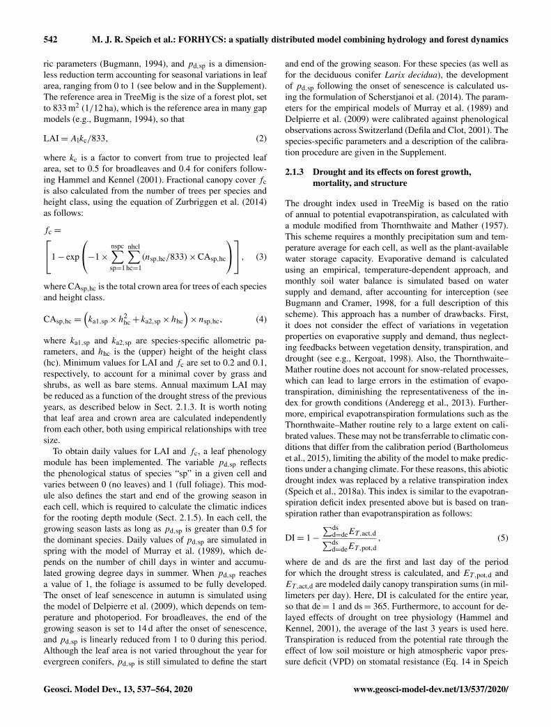
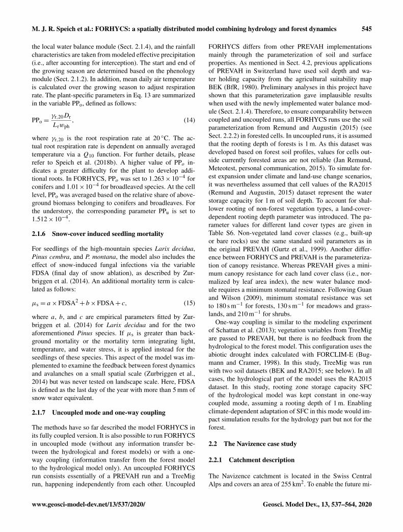
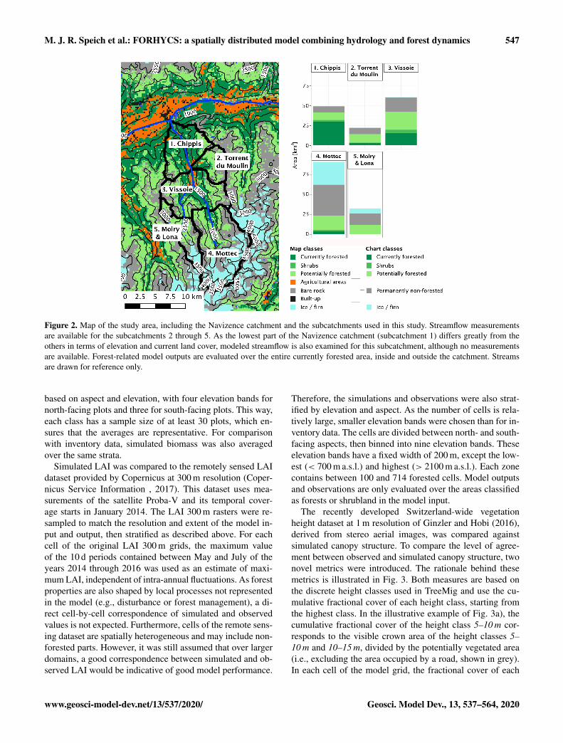
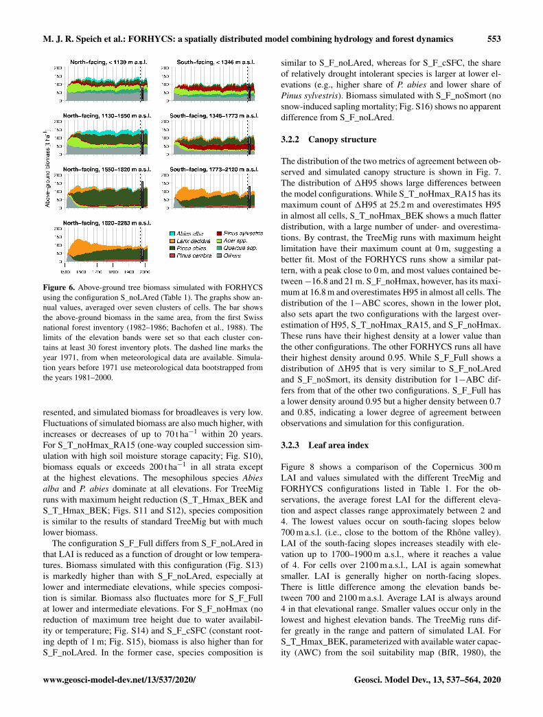
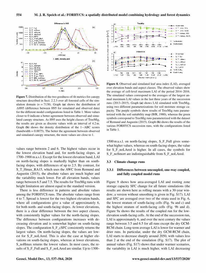
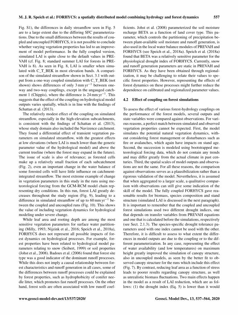


![Evolution of the Stomatal Regulation of Plant Water ...Update on Stomatal Evolution Evolution of the Stomatal Regulation of Plant Water Content[OPEN] Timothy J. Brodribb* and Scott](https://static.fdocuments.us/doc/165x107/5e87e202c27a1d71d24f112b/evolution-of-the-stomatal-regulation-of-plant-water-update-on-stomatal-evolution.jpg)


![Stomatal Defense a Decade Later1[OPEN] - Plant Physiology · Update on Stomatal Defense Stomatal Defense a Decade Later1[OPEN] Maeli Melotto*, Li Zhang, Paula R. Oblessuc, and Sheng](https://static.fdocuments.us/doc/165x107/5eddc0a3ad6a402d6668efaa/stomatal-defense-a-decade-later1open-plant-update-on-stomatal-defense-stomatal.jpg)

