
Forecasting Inflation via Electronic Markets Results from ...
40
February 2002 Forecasting Inflation via Electronic Markets Results from a Prototype Experiment Michael Berlemann BULGARIAN NATIONAL BANK dp/20/2002 dp/20/2002 dp/20/2002 dp/20/2002 dp/20/2002 DISCUSSION PAPERS
Transcript of Forecasting Inflation via Electronic Markets Results from ...
February 2002
Forecasting Inflation via ElectronicMarkets Results from a PrototypeExperiment
Michael Berlemann
BULGARIAN NATIONAL BANKdp
/20/
2002
dp/2
0/20
02dp
/20/
2002
dp/2
0/20
02dp
/20/
2002
DISC
USSIO
N PA
PERS
2
dp/
20/2
002
© Bulgarian National Bank, February 2002
ISBN 9954≠9791≠52≠1
Accepted October 2001.
Printed in BNB Printing Center.
Views expressed in materials are those of the authors and do not necessarily
reflect BNB policy.
Send your comments and opinions to:Publications DivisionBulgarian National Bank1, Alexander Battenberg Square1000 Sofia, BulgariaTel.: 9145/1271, 1351, 1906Fax: (359 2) 980 2425e-mail: [email protected]
Website: www.bnb.bg
DISCUSSION PAPERSEditorial Board:Chairman: Garabed MinassianMembers: Roumen Avramov
Georgi PetrovSecretary: Lyudmila Dimova
3
Disc
ussion P
aper
s
Contents
Introduction........................................................................................... 5
Why Bother with Future Inflation?..................................................... 6
Conventional Forecasting Methods .................................................... 7
The Econometric Approach ........................................................ 8The Expectations Approach ...................................................... 10Conclusions ................................................................................. 13
The Design of an Electronic Inflation Forecasting Market ............14
Market Admittance .................................................................... 14Market Setup .............................................................................. 15Market Liquidation .................................................................... 16Trading within the Inflation Market ......................................... 17
Results from the Prototype Market .................................................. 19
Basic Market Data and Properties of the Prototype Market .. 19The Mean Market Inflation Forecast ....................................... 23Measuring Uncertainty of the Mean Inflation Forecast .......... 28
Normally Distributed Forecasts and Further Applications ........... 29
Application I: Calculation of the Probability of Inflation Scenarios, No Contract Is Traded for ............. 31Application II: Calculation of Confidence Intervals and Modified Fan Charts ................................. 32
Discussion of the Prototype Marketís Design and Its Results ....... 33
Summary and Outlook ....................................................................... 35
References ............................................................................................37
4
dp/
20/2
002 SUMMARY. FORECASTS OF MACROECONOMIC VARIABLES AS THE INFLATION RATE
SERVE AS IMPORTANT GUIDELINES FOR THE PRIVATE AS WELL AS THE PUBLIC SECTOR.AT LEAST CENTRAL BANKS THAT ADOPTED AN INFLATION TARGETING REGIME ARE IN
URGENT NEED OF HIGH QUALITY INFLATION FORECASTS. ACCURATE INFLATION FORE-CASTS ARE ALSO NEEDED WITHIN PRIVATE SECTOR WAGE NEGOTIATIONS. IN THIS PAPER
WE PRESENT A NEW METHOD TO PREDICT FUTURE INFLATION VIA CONDUCTING ELEC-TRONIC MARKETS. WE SHOW AT THE EXAMPLE OF A PROTOTYPE MARKET HOW THE
MARKET DATA OF SUCH AN EXPERIMENTAL MARKET CAN BE USED TO GENERATE PREDIC-TIONS OF THE FUTURE INFLATION RATE. WE ALSO SHOW THAT THE MARKET DATA PRO-VIDE IMPORTANT EVIDENCE ON THE DISTRIBUTION OF INFLATION EXPECTATIONS.
JEL classification: C93, E37
Keywords: Inflation Forcasting, Inflation Targeting, Electronic Markets
The author thanks Forrest Nelson, Joyce Berg and the Iowa Electronic Markets team for theirgreat support in planning and conducting the market. He is also grateful for comments fromForrest Nelson on an earlier version of this paper.
Dr. rer. pol. Michael Berlemann, Chair for Economics, esp. Money, Credit and Currency,Faculty of Business Management and Economics, Dresden University of Technology, D-01069Dresden, Tel.: 0351-463-35904, E-mail: [email protected]
5
Disc
ussion P
aper
s
IntroductionElectronic market research started to evolve in the aftermath of a market
experiment set up by a group of researchers from the University of Iowa. Onthe occasion of the 1988 presidential election in the United States they orga-nized an electronic market where shares on the candidates for presidentshipwere traded. This first political stock market proved to be highly successfulin predicting the outcome of the presidential election.1 Motivated by the goodresults the Iowa Electronic Markets (IEM) were founded to organize elec-tronic markets regularly. Since 1988 IEM organized a large number of mar-kets, most of them on the occasion of political elections.2 Altogether the mar-kets were quite successful in predicting the electoral outcome.3 Initiated andstrongly supported by members of IEM, political stock markets were alsoorganized outside the U.S., for instance in Austria, Canada, Denmark, Ger-many, Italy, the Netherlands and Turkey. Though the electoral systems andthe political landscapes in these countries are somewhat more complex thanin the U.S. the most of these markets provided well forecasting results. A re-cent meta study by Berlemann and Schmidt (2001) for 28 German politicalstock markets showed that on average the markets proved to be even moresuccessful in predicting the electoral outcome than the polls of public opin-ion research institutes.
Political stock markets’ success in predicting political events made us be-lieve that it could be fruitful to think about transferring the idea of usingelectronic markets as a forecasting device to genuine economic events. Weargue that a well-designed electronic market should also be able to providesome reasonable forecast of macroeconomic variables. In this paper we fo-cus on the question, how electronic markets can be used to forecast futureinflation. Using binary options, we develop a prototype-market for forecast-ing inflation. We also present empirical results from a recent pilot experimentwith an inflation forecasting market and show how the market reveals wor-thy information on future inflation and the probability of different inflationscenarios.
1 For a description of the 1988 presidential stock market compare Forsythe et al. (1992).
2 For an overview on the political stock markets organized by IEM compare Berg et al. (1997).More information on IEM is provided on the IEM-Homepage: http://www.biz.uiowa.edu/iem.
3 It should be noted that the main objective of electronic market research was to ‘produce’market data in an at least somewhat controlled environment to analyze aspects like individualmarket behavior, information aggregation within markets or informational efficiency of mar-kets. In the beginning of electronic market research forecasts were only some kind of by-prod-uct of conducting markets. Even if the data from the markets we propose can be used studymarket behavior, too, we will solely focus on the forecasting aspect in this paper.
6
dp/
20/2
002 The paper is organized as follows: In the second section we deal with the
question why forecasting inflation is an important issue. The third sectionbriefly reviews conventional methods of forecasting inflation. In sectionFour the basic design of an inflation forecast market is developed. We alsoshow why we expect this market to produce some high quality inflation fore-cast in this section. Section Five presents empirical results from a recent pi-lot experiment with an inflation forecasting market. In section Six we showsome further evaluations of the market data under the assumption of nor-mally distributed expectations. In section Seven we compare the electronicmarkets system with conventional forecasting methods and discuss unre-solved questions and possible further extensions. Section Eight summarizesthe main results and gives a short outlook on future research ideas.
Why Bother with Future Inflation?The starting point of the following expositions is the question, why
people care about future inflation or – at least – why they should care aboutit. Inflation, defined as permanent increases of the aggregate price level, istypically supposed to cause several effects that might positively or nega-tively influence personal and social welfare. The reason why the goal of astable price level is a major objective of economic policy all around theworld is that the negative distributional and allocative effects of (expectedand unexpected) inflation are typically supposed to dominate the positiveones.4
Nowadays, in the most countries the central banks are concerned with thegoal of guaranteeing stable prices. In order to so, an increasing number ofcentral banks have adopted a so-called ‘inflation targeting regime’ during thelast decade. Inflation targeting is a framework for monetary policy that ischaracterized by announcing an explicit official target or at least a targetrange for the inflation rate for some predefined period of time. In an inflationtargeting framework there is a strong commitment of the monetary authorityto concentrate on holding inflation within the target range as the primarygoal of monetary policy. An important element of such a strategy is a highdegree of transparency with respect to the central bank’s objectives as wellas to the undertaken actions to fulfill them. Since monetary policy affects theinflation rate with a lag of some 18 – 24 months, monetary policy has to beforward looking. Svensson (1997) showed that the implementation of an in-flation targeting regime for monetary policy implies to use the inflation fore-
4 Sill (1999), p. 5.
7
Disc
ussion P
aper
s
cast as intermediate target in a way that monetary policy should be tightenedwhen actual inflation expectations exceed the target level and the other wayround. Even if a monetary authority follows a different monetary policystrategy but still primarily tries to guarantee stable prices it often uses infla-tion expectations as an important indicator, at least with respect to the cred-ibility of its monetary policy strategy. Whenever a central bank that is com-mitted to low inflation observes high inflation expectations, the actual mon-etary strategy seems not to be highly credible. A central bank might take thisas a signal to think over the actual policy strategy.
Even if central banks in industrial countries were quite successful infighting inflation within the last decade, inflation was not eliminated at all.There is even no guarantee that the actually low levels of inflation will lastwithin the future. Thus also private institutions are interested in future infla-tion to anticipate expected changes in the aggregate price level in order toprevent negative distributional effects of unexpected inflation. Banks carryan interest in anticipating future inflation in credit contracts. Labor unionstry to anticipate future inflation during the wage negotiations to prevent theirmembers from suffering unexpected losses in real wages etc.
Last but not least researchers are interested in the way how people makeindividual forecasts on macroeconomic variables like inflation. Empiricaldata on this aspect are worthy to test different hypotheses on the formation ofexpectations, thereby providing evidence how to model the private sector inmacroeconomic models.
Altogether we may conclude that governmental as well as private institu-tions are in urgent need of forecasts of future inflation. In fact, by far themost central banks care very much about future inflation and often invest alot of resources into forecasting activities. The same is true for private banksand firms.
Conventional Forecasting MethodsThere are two basic concepts of dealing with the problem of forecasting
future inflation. The first concept, we will call it the ‘econometric approach’in the following, tries to generate forecasts on the basis of actual and histori-cal empirical data using econometric techniques. The basic idea of this ap-proach is that there is some theoretical model explaining by which factorsinflation is determined. Whenever we believe to know, which is the correctmodel and we have the necessary data at hand we should be able to producesome reasonable forecast of future inflation. The second concept of forecast-ing inflation, we will call it ‘expectations approach,’ does not care about the
8
dp/
20/2
002 question which is the appropriate theory allowing to predict future inflation.
The expectations approach simply suggests that a certain subgroup ofpeople, caring about future inflation, knows enough about the true determi-nants of price level changes to be able to predict future inflation well on av-erage. Thus it is sufficient to measure the inflation expectations of an in-formed subgroup without knowing which methods are used for the indi-vidual forecasts.
It is easy to imagine that both, the econometric and the approaches ofmeasuring inflation expectations are themselves quite heterogeneous. In thefollowing we will give a brief overview on the typically used methods.
The Econometric ApproachWhen using econometric methods for forecasting purposes we typically
start out from some theoretical model how the economy works. It is out ofthe question that an economy is an extremely complex and highly dynamicsystem. On the one hand the model should capture as many important rela-tionships between the relevant macroeconomic variables as possible to besuccessful in forecasting. On the other hand a growing complexity of themodel typically increases the problems to handle it and to use econometricforecasting methods. In the end the problem to solve typically is to determinewhich econometric model allows to reach a given average forecasting suc-cess by the lowest effort.
As it was argued earlier in this paper, most central banks are in urgentneed of precise inflation forecasts. Thus it is no surprise that central bankstypically invest a lot of resources into forecasting activities. Most centralbanks use highly complex macroeconometric core-models that sometimesconsist of more than a hundred of equations. While the basic inflation fore-casting concepts of the central banks are typically well documented,5 it is of-ten hard to get detailed information on how the forecasts are done.6 In anycase the models are far too complex to be reviewed at length in this paper.
The basic problem with purely econometric models is that they try to es-timate future inflation via past observations of inflation itself and other real-izations of macroeconomic variables. These models are backward-looking
5 Compare e.g. Poloz, Rose and Tetlow (1994) for the Bank of Canada’s, Goodhart (2001) for
the Bank of England’s, Cassino et al. (1997) and Drew and Hunt (1998) for the Bank of NewZealand’s, Jansson and Vredin (2001) for the Swedish Riksbank’s and Brayton et al. (1997) forthe Federal Reserve Bank’s forecasting system.
6 An exception is the detailed report on the Bank of England’s forecasting system (Bank ofEngland, 1999).
9
Disc
ussion P
aper
s
thereby neglecting the Lucas-Critique. It is easy to understand that suchmodels will hardly be able to predict changes in inflation expectations thathave to do with news like announcements of future policy changes, at least inthe long run.7 It is also hard to say something about the probability of differ-ent inflation scenarios on the basis of these models.
Even if the used forecasting models differ quite heavily from case tocase, some regularities can be observed. Most central banks do not rely on asingle econometric inflation forecasting model. Often the core-model issupplemented by less complex models to generate forecasts for exogenousvariables, to adjust the core model for short-term disequilibria or to simplycontrol for the plausibility of the core-model’s predictions. The Bank of En-gland as well as the Federal Reserve Bank use – among others – Phillipscurve models for this purpose.8 Even if central banks invest a lot of resourcesinto econometric forecasting models they often do not completely rely onthese models’ forecasts. George (1999, p. V), the Bank of England’s Gover-nor, states in this respect:
“The Bank’s use of economic models is pragmatic and plural-ist. In an ever-changing economy, no single model can possiblyassimilate in a comprehensive way all the factors that matter forpolicy. Forming judgements about those factors, and their implica-tions for policy, is the job of the Committee, not something thatcan be abdicated to models or even to modelers. But economicmodels are indispensable tools in that process.”
Thus individual beliefs and judgments often play an important role evenin inflation forecasts that are based upon econometric models.
Since the inflation forecasts from econometric models of central banksare often not published,9 it is hard to judge the quality of this type of fore-casts. Even if the forecasts are publicly announced, often the time series aretoo short to assess the forecast’s quality empirically. In a recent studyAtkeson and Ohanian (2001) analyzed in how far different types of Phillips
7 Ragan (1995), p. 4.
8 Compare Bank of England (1999), p. 77-92 or Stock and Watson (1999) for a description ofPhillips curve models.
9 The Bank of England publishes its inflation forecasts within the regular inflation reports.Nevertheless, the mean inflation forecast is somewhat hard to assess because the forecasts arepresented in the form of so-called fan-charts. Somewhat surprising neither the empirical dataunderlying this fan-chart nor the mean inflation forecast is provided numerically. The FederalReserve Bank treats its own inflation forecasts as confidential and therefore publishes themwith a lag of five (!) years in the so-called Greenbook.
10
dp/
20/2
002 curve models, as they are used by the Federal Reserve Bank or the Bank of
England, are useful for forecasting inflation. Using US data they show thatthe predictions of these models were worse than simply assuming that infla-tion will be the same over the next year as it has been over the last year. In-terestingly enough, Atkeson and Ohanian (2001) also found that even theFederal Reserve Bank’s inflation forecasts, published in the Greenbook,proved not to be better than the naive forecast that everything stays the samein the future.
The Expectations ApproachAs it was described earlier, the expectations approach does not care about
the question which is the appropriate model of the economy. The basic ideaof the expectations approach is that many people care – or at least shouldcare – about inflation. Since inflation directly decreases purchasing power ofall monetary assets, people owning or intending to buy these assets willmake individual predictions on future inflation. The individual beliefs on fu-ture changes in the price level might differ heavily because of heterogenousinformation sets and different ways of interpreting them (i.e. individualsmight use different theoretical ‘models’ for their forecasts). If individual ex-pectations are formed rationally they should be a good predictor for futureinflation. Thus the basic question to be answered is how to measure inflationexpectations.
Again there are two basic concepts how to solve the problem of measur-ing inflation expectations: conducting inflation expectation surveys or deriv-ing inflation expectations from financial market data. In the following wewill briefly describe both approaches.
Inflation Expectation SurveysThe most direct way to assess inflation expectations is to conduct qualita-
tive or quantitative inflation expectation surveys.The most commonly applied qualitative survey method is the so-called
‘net balance statistic’. In these surveys the respondents have to guesswhether inflation will ‘go up’, ‘stay the same’ or ‘go down’ within a certainperiod of time. In its simplest form the net balance value is then obtained bysimply subtracting the proportion of respondents that supposed the inflationrate to decrease from the one that predicted increasing inflation.10
10 For a more detailed discussion of the net balance statistics compare Batchelor (1986) and
Foster and Gregory (1977).
11
Disc
ussion P
aper
s
In direct quantitative surveys the respondents have to state numerical val-ues for expected inflation.11 The results then have to be aggregated by someprocedure. Typically the answers of the respondents are weighted equally tocalculate the mean inflation expectation. Often quantitative surveys are con-ducted separately for different groups in society, e.g. households, manufac-turers or professional forecasters.12
In a expert’s report on the measurement of inflation expectations, madeout on the occasion of the recent adoption of an inflation targeting regime inSouth Africa, Laubscher and Schombee (1999) evaluated experiences of 6inflation targeting countries and the United States with different inflation ex-pectations surveys. Their main results can be summarized as follows:
• Direct quantitative inflation expectation surveys typically performbetter than qualitative surveys. The net balance statistics createssomewhat erratic forecasts correlating poorly with real inflation. Inaddition to that net balance statistics turned out to be biased down-wards in times of high inflation and high uncertainty and vice versa.
• The best results with respect to predicting core inflation and futurenominal wage growth can be obtained by household and consumersurveys while the results of surveys of professional forecasters andeconomists perform better in predicting future interest rate move-ments.
Nevertheless there are various unresolved problems with quantitative in-flation expectation surveys due to the typical survey errors:
• There is an urgent need of having a representative sample to reducesampling errors. It is a long known fact that such a sample is hard toobtain. As Laubscher and Schombee (1999, p. 16) report, the re-sponse rates in inflation expectation surveys are generally low (25 upto 35%). This makes it nearly impossible to obtain a representativesample.
11 Prominent examples for quantitative inflation expectations surveys are the Livingston Sur-
vey and the Survey of Professional Forecasters, conducted by the Federal Reserve Bank ofPhiladelphia.
12 In an analysis for US data Gramlich (1986) found the surprising result that the quantitativeexpectation surveys of consumers, namely the University of Michigan ISR consumer survey,performed significantly better than the Livingston survey of professional forecasters in fore-casting future inflation. Similar results were found by Roberts (1998). In addition to that thelower educated and poorer consumers performed better in forecasting inflation than those ofthe higher educated and richer consumers on average. Thus different groups in society seem tohave different levels of information or at least do react differently on certain types of informa-tion.
12
dp/
20/2
002 • The questions the respondents have to answer within the survey have
to be formulated very carefully to avoid answering biases. The sameis true for the used questioning technique. Especially the often usedtelephone surveys are prone to different sorts of biases.
• The timing of inflation expectation surveys is extremely important.All respondents should be asked within a short period of time to as-certain that the basic information set is the same.
• One of the most important problems is that the respondent typicallyhave no incentive to reveal their true expectations. Often the respon-dents are rewarded financially for answering and thus have a strongincentive to take part in the survey even if they have no informationon future inflation at all or do not care about the topic. In addition tothat the interviewers might motivate uninformed respondents to an-swer nevertheless because they are paid per interview and typicallyare interested in minimizing their transaction costs.
• Given that the survey typically includes a good number of very poorinformed respondents it seems to be somewhat questionable to attachthe same weight to each individual interview. This aggregation prob-lem can hardly be solved because the level of information of a re-spondent can not be measured objectively.
Thus there are several theoretical arguments explaining why inflation ex-pectation surveys do not predict future inflation very accurately.
Gauging Inflation Expectations from Financial MarketDataTwo major problems of the direct approach of measuring inflation expec-
tations are, as pointed out earlier, that the interviewed people have no incen-tive to reveal their true expectations and the aggregation problem. Both prob-lems can be solved by means of gauging inflation expectations from finan-cial market data. According to the Fisher relation (compare Fisher (1930))
imt = Et [π m
t ] + r mt (1)
inflation expectations at time t with respect to time m, denoted by Et[πmt ] , af-
fect nominal interest rates i. The basic problem to solve when using theFisher equation to extract inflation expectations from financial market data ishow to get information on the corresponding real interest rate r.
Inflation expectations are easy to extract from market data when there isa well-functioning market for real (indexed) bonds. In that case we can sim-
13 Compare Deacon and Derry (1994) or Svensson (1994).
13
Disc
ussion P
aper
s
ply subtract the real interest rate from the nominal interest rate of equal-ma-turity bonds to obtain inflation expectations.13 Since there are only a fewcountries with markets for indexed bonds this method can rarely be used.
If there is no market for indexed bonds it is possible to gauge inflationexpectations from the term structure of (nominal) interest rates on govern-ment bonds14 under certain circumstances. Ex-post inflation within the periodfrom t to m can be described by
π mt = Et[π m
t ] + ε mt (2)
with ε being the forecast error. Combining equation (2) and (1) we obtain
π mt = im
t + r mt + ε m
t (3)
Using equation (3) for bonds with two different maturities m and n withm > n leads to
π mt � π n
t = (imt � in
t ) � (r mt � r n
t ) + (ε mt � ε n
t ) (4)
Under the assumption of rationally formed expectations the expectationerrors are zero on average. If we further assume that the real interest rate isnot changing between time n and m or we at least know on how much it isassumed to change within this period, we are able to calculate the financialmarket’s inflation forecast.15
Altogether the empirical results on the predictive quality of the above de-scribed method are not very promising. While Mishkin (1990,1991) andEstrella and Mishkin (1997) found at least long term forecasts to be some-what reliable, Jochum and Kirchgassner (1999) show that even these resultsdo not hold when taking non-stationarity of at least some of the data into ac-count.
ConclusionsIt was shown that all described methods of forecasting inflation have
their advantages and their drawbacks. Thus it is not surprising that none ofthem dominates in the practice of forecasting. Most central banks rely on amixture of the concepts and often decide somewhat discretionary on the ap-propriate forecast. We might interpret this as some kind of distrust in con-ventional forecasting methods. Thus further research in methods of measur-ing future inflation seems to be useful and necessary.
14 Governmental bonds are used because they are assumed to have the lowest degree of de-
fault risk, thereby assuring that the nominal interest rates contain no risk premium.15 For an overview on more advanced methods to extract inflation forecasts from financial
instruments compare e.g. Soderlind and Svensson (1997).

14
dp/
20/2
002
16 The students in these two courses got an extra endowment of 5 euro when investing at least
ten euro on their own as an additional incentive to take part in the market. It should also be
The Design of an Electronic InflationForecasting Market
In the face of the fact that conventional methods of forecasting did notprove to be highly reliable in predicting future inflation, yet, it might be use-ful to think about alternative forecasting methods. Our proposal is to usewell-designed electronic markets for this purpose. The forecasting systemwe propose is some kind of combination of the two expectation approaches(expectation surveys, use of market data) we already discussed.
Principally, electronic market research belongs to the field of experimen-tal economics. An electronic market is a virtual market where shares on cer-tain events are traded. Typically electronic markets are organized via internetand on the basis of real-money transactions. In the following we will showhow an electronic market can be designed to forecast future inflation at theexample of a recently conducted prototype market.
Market AdmittanceElectronic markets are fully computerized markets. To be able to take
part in such a market, participants have to register for admittance viainternet, first. Besides providing some personal data during the process ofregistration, participants have to decide on their personal initial investments.Typically investments are somewhat restricted due to legislative restrictions.In the prototype market the minimum investment was 10 euro and the maxi-mum investment was 500 euro. The initial investments have to be coveredby the traders. All transactions in the market are based on real money. Eachparticipant can win or loose money in the market, depending on his or hersuccess in trading.
As soon as the initial investment has been transferred to the market orga-nizer (typically this is done via cash or bank transfer to a market account) theparticipant gets a trader-ID and a password to login the market. In addition tothat a trader account for the participant is created and his initial investment istransferred to the account.
Technical precondition for taking part in an electronic market is aninternet connection. Even if there were no formal restrictions for participa-tion in the prototype market the most traders were students of economics andbusiness administration at Dresden University of Technology. The marketwas presented within two university courses on monetary economics16 and
15
Disc
ussion P
aper
s
was announced in some other university courses.
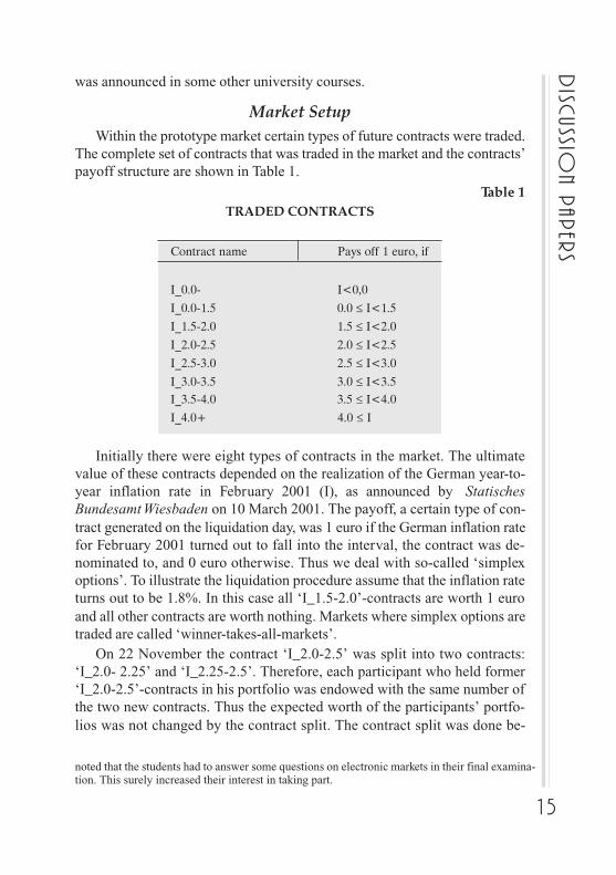
Market SetupWithin the prototype market certain types of future contracts were traded.
The complete set of contracts that was traded in the market and the contracts’payoff structure are shown in Table 1.
Table 1TRADED CONTRACTS
Contract name Pays off 1 euro, if
I_0.0- I<0,0
I_0.0-1.5 0.0 ≤ I<1.5
I_1.5-2.0 1.5 ≤ I<2.0
I_2.0-2.5 2.0 ≤ I<2.5
I_2.5-3.0 2.5 ≤ I<3.0
I_3.0-3.5 3.0 ≤ I<3.5I_3.5-4.0 3.5 ≤ I<4.0
I_4.0+ 4.0 ≤ I
Initially there were eight types of contracts in the market. The ultimatevalue of these contracts depended on the realization of the German year-to-year inflation rate in February 2001 (I), as announced by StatischesBundesamt Wiesbaden on 10 March 2001. The payoff, a certain type of con-tract generated on the liquidation day, was 1 euro if the German inflation ratefor February 2001 turned out to fall into the interval, the contract was de-nominated to, and 0 euro otherwise. Thus we deal with so-called ‘simplexoptions’. To illustrate the liquidation procedure assume that the inflation rateturns out to be 1.8%. In this case all ‘I_1.5-2.0’-contracts are worth 1 euroand all other contracts are worth nothing. Markets where simplex options aretraded are called ‘winner-takes-all-markets’.
On 22 November the contract ‘I_2.0-2.5’ was split into two contracts:‘I_2.0- 2.25’ and ‘I_2.25-2.5’. Therefore, each participant who held former‘I_2.0-2.5’-contracts in his portfolio was endowed with the same number ofthe two new contracts. Thus the expected worth of the participants’ portfo-lios was not changed by the contract split. The contract split was done be-
noted that the students had to answer some questions on electronic markets in their final examina-tion. This surely increased their interest in taking part.
16
dp/
20/2
002 cause it was observed that the former ‘I_2.0-2.5’-contract had been traded
for quite high prices, thus indicating that the participants attached a highprobability to the event that the inflation rate would have been in between 2and 2.5%. To be able to forecast the inflation rate more accurately, the formercontract ‘I_2.0-2.5’ was divided into two new contracts covering the sameinterval.
Market LiquidationThe prototype market was liquidated soon after the German inflation rate
for February 2001 was announced on 10 March. This was done by the fol-lowing two-step procedure:
1. Each participant got back the money he held on his market account inthe end of the market.
2. Each participant got the liquidation value of the portfolio of contracts,he held in the end of the market.
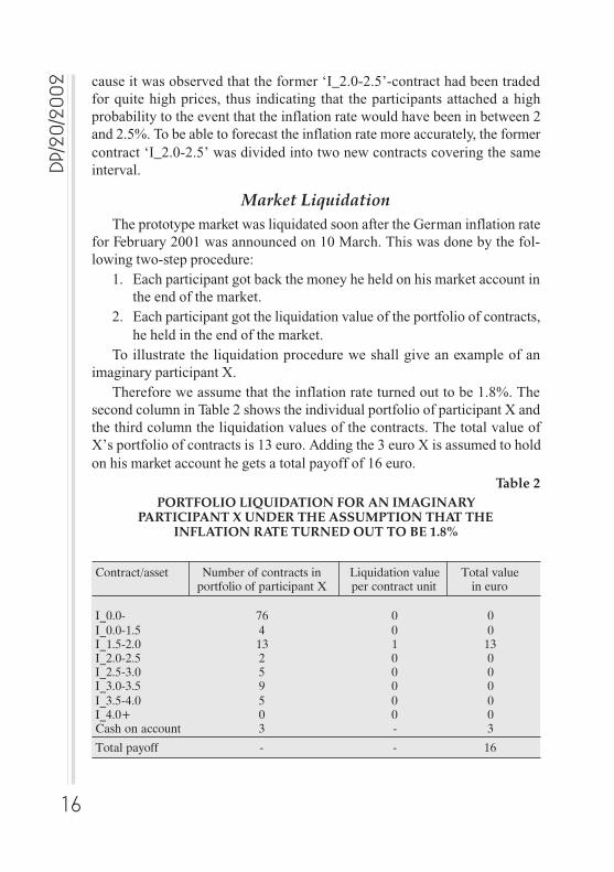
To illustrate the liquidation procedure we shall give an example of animaginary participant X.
Therefore we assume that the inflation rate turned out to be 1.8%. Thesecond column in Table 2 shows the individual portfolio of participant X andthe third column the liquidation values of the contracts. The total value ofX’s portfolio of contracts is 13 euro. Adding the 3 euro X is assumed to holdon his market account he gets a total payoff of 16 euro.
Table 2PORTFOLIO LIQUIDATION FOR AN IMAGINARY
PARTICIPANT X UNDER THE ASSUMPTION THAT THEINFLATION RATE TURNED OUT TO BE 1.8%
Contract/asset Number of contracts in Liquidation value Total valueportfolio of participant X per contract unit in euro
I_0.0- 76 0 0I_0.0-1.5 4 0 0I_1.5-2.0 13 1 13I_2.0-2.5 2 0 0I_2.5-3.0 5 0 0I_3.0-3.5 9 0 0I_3.5-4.0 5 0 0I_4.0+ 0 0 0Cash on account 3 - 3
Total payoff - - 16
17
Disc
ussion P
aper
s
Trading within the Inflation MarketThe prototype market was open for transactions at any time during the
market period, i.e. from 9 October 2000 up to 15 March 2001. Upon enteringthe market and any time thereafter until the market closed a participant couldbuy unit portfolios (so-called ‘bundles’) from the market organizer for theprice of 1 euro. Each unit portfolio consisted of one of each type of contracts.Thus a bundle in the inflation market included 8 contracts initially and 9 con-tracts after the contract split. Complete unit portfolios could also be soldback to the market organizer during the market period for the price of 1 euroeach. Selling and buying unit portfolios from or to the market organizer areprimary market transactions.
Together with the already described market-liquidation procedure thepricing of the unit portfolios guaranteed that the market is a zero-sum-gamefor the market organizer. All initial investments were paid back to the partici-pants. The market was typically no zero sum game for the individual partici-pant since he could win or loose money, depending on his success in tradingwithin the market.
To be able to realize profits in the market, a participant had to tradewithin the secondary market, i.e. he had to buy or sell contracts from or toother participants.17 The secondary market was organized as a so-called‘double-auction-market’. The participants could issue offers to buy (bids) oroffers to sell (asks) contracts. When using the first type of transactions, theso-called ‘limit orders’, the traders had to choose the order type (bid or ask),the contract type (e.g. ‘I_0.0- 1.5’), the number of contracts he wants totrade, the transaction price and finally the expiration date of the order. Limitorders were maintained in separate bid and ask queues ordered first by offerprice and then by the time of issuance. Whenever an offer entered one of thequeues it remained there until the offer turned out to be unfeasible (e.g. be-cause of a lack of liquidity to realize a buying transaction), was withdrawnby the trader, reached its expiration date or was carried out. Orders were car-ried out whenever bid- and ask-prices overlapped.
The market software provided several facilities for the traders to obtaininformation on the market. On the one hand, the trader got personal informa-tion about his market account, current portfolio and the orders he submitted.On the other hand, there was information about the highest bids to buy andlowest asks to sell for each traded contract type. Similar to real stock markets
17 For a more detailed description of the trading system of the Iowa Electronic Markets-soft-
ware compare Forsythe et al. (1991), pp. 74 – 78.
18
dp/
20/2
002
18 If we take a closer look at the situation, the described arbitrage strategy is not totally risk-
free because of the risk that during the arbitrage transactions someone may withdraw his order.If we take into account that realizing arbitrage transactions do take only a few seconds of time,this risk is very small and thus can be neglected.
the trader obtained no information on how much contracts he would havebeen able to buy or sell at actual prices. He could only be sure to be able tosell or buy at least one contract at actual prices. To do so the traders coulduse the second type of transaction, the so-called ‘market orders’. Market or-ders were always carried out immediately at current prices. Thus the traderhad only to specify the contract type, the order type (bid or ask) and the num-ber of contracts he wants to trade in this case.
Finally we should note that, different from real stock markets, short salesand purchases on margin were disallowed to secure the zero sum-game char-acter of the market.
Before we turn to the results of the inflation market, we will discusswhich basic trading strategies are possible. Principally we might think of thefollowing four types of possible strategies that might be combined in severalways:
1. the arbitrage strategy,2. the expectations strategy,3. the risk-adjusted expectations strategy and4. the speculative strategy.The arbitrage strategy focuses on realizing risk-free profits. Arbitrage
operations are possible in the inflation market whenever the sum of all actualbids to buy is above 1 euro or the sum of all asks to sell is below 1 euro. Inthe first case a trader can buy a unit portfolio from the market organizer atthe price of 1 euro and sell it immediately at current prices within the sec-ondary market. In the latter case a trader can buy a unit portfolio at currentprices on the secondary market and sell it on the primary market at the priceof 1 euro. In both cases he earns a risk-free profit.18
The second strategy, the expectations strategy, requires to build some ex-pectation on the realization of the event that is determining the final liquida-tion values of the contracts. In its simplest form the trader starts out from theassumption that his expectation will coincide with the realization of theevent. In this case he will buy only those contracts, he assesses to be under-valued by the market, and sell all contracts he supposes to be overvalued.
A third strategy is some kind of variation of the simple expectations strat-egy. Following the risk adjusted expectations strategy requires to take into
19
Disc
ussion P
aper
s
account that the subjective expectations on the realization of the event mightbe wrong or at least somewhat distorted. Similar to a trader following thesimple expectations strategy he will buy contracts he supposes to be heavilyundervalued. But different from the simple strategy he will weigh up thepossible profits if his expectations proof to be correct against the risk thatthey are wrong. Therefore ceteris paribus a trader following the risk adjustedexpectations strategy will sell a contract earlier when prices rise than a traderfollowing the simple expectations strategy.
Under the speculative strategy there is no need to know very much aboutthe ‘true’ realization of the event determining the liquidation values of thetraded contracts. Traders that are keen on speculative profits are trying tomake use of short- or middle-term trends. Thus a speculative trader will holda contract even if he suggests that is already overvalued as long as he expectsthat prices will go on rising. This strategy is quite risky because there is noguarantee for the trader to be able to sell the contracts before the speculativebubble bursts.
Results from the Prototype Market
Basic Market Data and Properties of the PrototypeMarket
Initial Investments and Final PayoffsBefore we present the forecasting results of the prototype market we
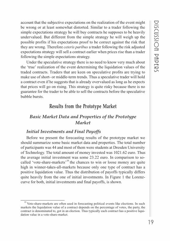
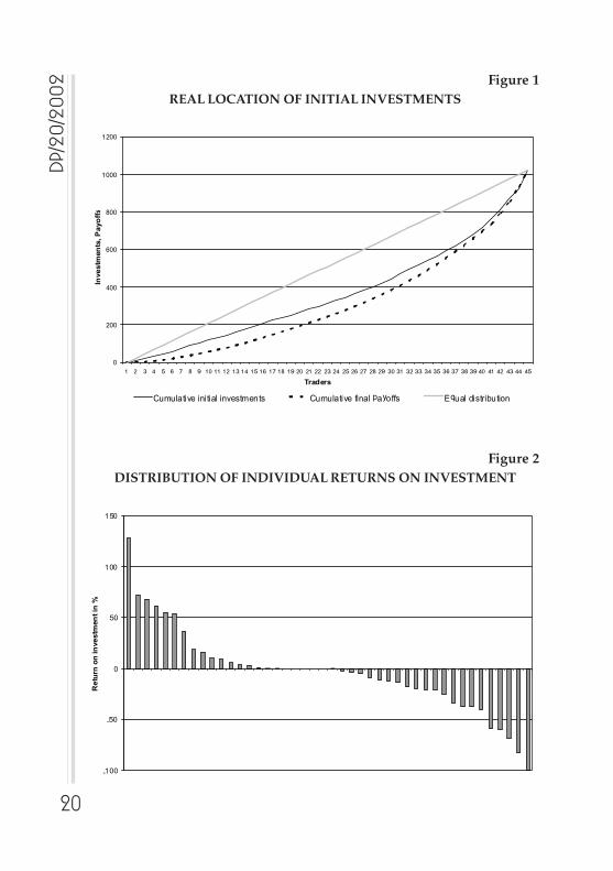
should summarize some basic market data and properties. The total numberof participants was 44 and most of them were students at Dresden Universityof Technology. The total amount of money invested was 1021.62 euro. Thusthe average initial investment was some 23.22 euro. In comparison to so-called ‘vote-share-markets’19 the chances to win or loose money are quitehigh in winner-takes-all-markets because only one type of contract has apositive liquidation value. Thus the distribution of payoffs typically differsquite heavily from the one of initial investments. In Figure 1 the Lorenz-curve for both, initial investments and final payoffs, is shown.
19 Vote-share-markets are often used in forecasting political events like elections. In such
markets the liquidation value of a contract depends on the percentage of votes, the party, thecontract is denominated to, got in an election. Thus typically each contract has a positive liqui-dation value in a vote-share-market.
20
dp/
20/2
002 Figure 1
REAL LOCATION OF INITIAL INVESTMENTS
Figure 2DISTRIBUTION OF INDIVIDUAL RETURNS ON INVESTMENT
0
200
400
600
800
1000
1200
1 2 3 4 5 6 7 8 9 10 11 12 13 14 15 16 17 18 19 20 21 22 23 24 25 26 27 28 29 30 31 32 33 34 35 36 37 38 39 40 41 42 43 44 45
Traders
Investm
en
ts, P
ayo
ffs
Cumulative initial investments Cumulative final payoffs Equal distribution
-100
-50
0
50
100
150
Retu
rn o
n in
vestm
en
t in
%
21
Disc
ussion P
aper
s
We see that initial investments differed quite heavily from trader totrader, resulting in a Gini-coefficient of 0.29.20 After the market was closed,the inequality of the traders’ wealth increased heavily to a Gini-coefficient of0.57. Thus the traders’ success in trading was somewhat different. The distri-bution of the rates of return on investment, the traders realized, is shown inFigure 2.
It might be suggested that the traders with high degrees of informationrealize higher returns on investment than the low informed traders. Becauseit is hard to measure the degree of individual information we can not test thishypothesis directly. We do not find supporting evidence in favor of the hy-pothesis that traders investing more money (what might be a signal of highinformation) are earning higher profits. The very low positive correlationbetween initial investments and returns (r = 0.112) is highly insignificant(p = 0.471).
From Figure 2 it is easy to see that the number of traders that realizedpositive returns on investment was somewhat smaller than the one that real-ized losses within the market. Altogether we might suppose that individualinformation on the future inflation rate was at least somewhat dispersedamong the traders.
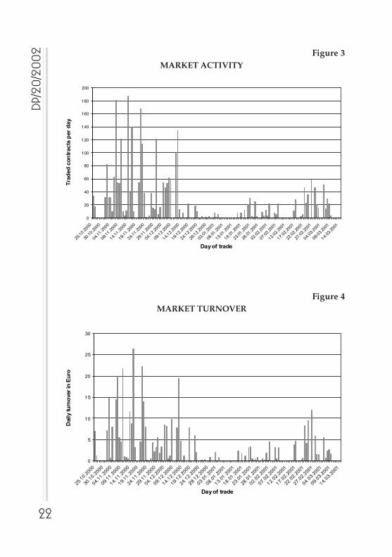
Market ActivityThe first transactions in the prototype market were done on 25 October
2000, i.e. about two weeks after opening up the market. This is due to thefact that the university courses and market advertising started in mid of Oc-tober. That is why we will focus on the period from 25 October up to 12March 2001 in the following expositions.
There was activity in the market during the whole market period withonly two short periods of very low activity. The first period of low activity(20 December 2000 up to 8 January 2001) was due to Christmas holidays.The second one (the week from 9 February up to 16 February 2001) startedin the end of the winter term at Dresden University of Technology.
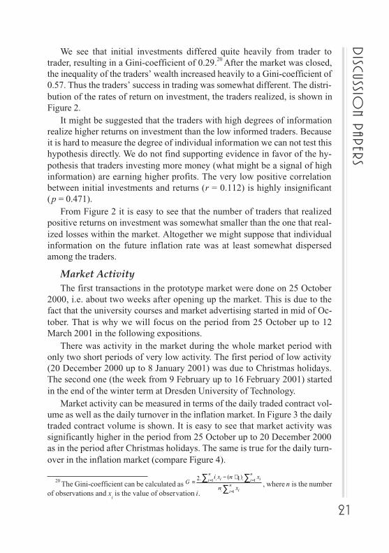
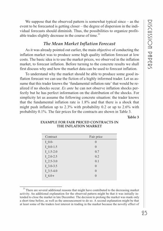
Market activity can be measured in terms of the daily traded contract vol-ume as well as the daily turnover in the inflation market. In Figure 3 the dailytraded contract volume is shown. It is easy to see that market activity wassignificantly higher in the period from 25 October up to 20 December 2000as in the period after Christmas holidays. The same is true for the daily turn-over in the inflation market (compare Figure 4).
20 The Gini-coefficient can be calculated as ∑
∑ ∑=
= =+−
=n
i i
n
i
n
i ii
xn
xnxiG
1
1 1
.
).1(..2, where n is the number
of observations and xi is the value of observation i.
22
dp/
20/2
002 Figure 3
MARKET ACTIVITY
Figure 4MARKET TURNOVER
0
20
40
60
80
100
120
140
160
180
200
25.10.2
000
30.10.2
000
04.11.2
000
09.11.2
000
14.11.2
000
19.11.2
000
24.11.2
000
29.11.2
000
04.12.2
000
09.12.2
000
14.12.2
000
19.12.2
000
24.12.2
000
29.12.2
000
03.01.2
001
08.01.2
001
13.01.2
001
18.01.2
001
23.01.2
001
28.01.2
001
02.02.2
001
07.02.2
001
12.02.2
001
17.02.2
001
22.02.2
001
27.02.2
001
04.03.2
001
09.03.2
001
14.03.2
001
Day of trade
Tra
ded
co
ntr
acts
per
day
0
5
10
15
20
25
30
25.10.2
000
30.10.2
000
04.11.2
000
09.11.2
000
14.11.2
000
19.11.2
000
24.11.2
000
29.11.2
000
04.12.2
000
09.12.2
000
14.12.2
000
19.12.2
000
24.12.2
000
29.12.2
000
03.01.2
001
08.01.2
001
13.01.2
001
18.01.2
001
23.01.2
001
28.01.2
001
02.02.2
001
07.02.2
001
12.02.2
001
17.02.2
001
22.02.2
001
27.02.2
001
04.03.2
001
09.03.2
001
14.03.2
001
Day of trade
Daily tu
rno
ver
in E
uro
23
Disc
ussion P
aper
s
We suppose that the observed pattern is somewhat typical since – as theevent to be forecasted is getting closer – the degree of dispersion in the indi-vidual forecasts should diminish. Thus, the possibilities to organize profit-able trades slightly decrease in the course of time.21
The Mean Market Inflation ForecastAs it was already pointed out earlier, the main objective of conducting the
inflation market was to produce some high quality inflation forecast at lowcosts. The basic idea is to use the market prices, we observed in the inflationmarket, to forecast inflation. Before turning to the concrete results we shallfirst discuss why and how the market data can be used to forecast inflation.
To understand why the market should be able to produce some good in-flation forecast we can use the fiction of a highly informed trader. Let us as-sume that this trader knows the ‘fundamental inflation rate’ that would be re-alized if no shocks occur. Ex ante he can not observe inflation shocks per-fectly but he has perfect information on the distribution of the shocks. Forsimplicity let us assume the following concrete situation: the trader knowsthat the fundamental inflation rate is 1.8% and that there is a shock thatmight push inflation up to 2.3% with probability 0.2 or up to 2.6% withprobability 0.1%. The fair prices for the contracts are shown in Table 3.
Table 3EXAMPLE FOR FAIR PRICED CONTRACTS IN
THE INFLATION MARKET
Contract Fair price
I_0.0- 0
I_0.0-1.5 0
I_1.5-2.0 0.7
I_2.0-2.5 0.2I_2.5-3.0 0.1
I_3.0-3.5 0
I_3.5-4.0 0
I_4.0+ 0
21 There are several additional reasons that might have contributed to the decreasing market
activity. An additional explanation for the observed pattern might be that it was initially in-tended to close the market in late December. The decision to prolong the market was made onlya short time before, as well as the announcement to do so. A second explanation might be thatat least some of the traders lost interest in trading in the market because the novelty effect of
24
dp/
20/2
002 Such a trader would buy all ‘I_1.5-2.0’-contracts at prices below 0.7 euro
and sell these contracts at prices above 0.7 euro, thereby fixing the marketprice to 0.7 euro. Similarly he would fix the prices of the other contracts totheir fair prices.
In reality we have to take into account that there might be no highly in-formed traders. Nevertheless we should expect that all relevant informationwithin the market is revealed by the market prices in the course of time. Weshould also expect that the quality of the market forecast depends on the trad-ers’ strategies. Forecast quality can be supposed to increase with an increas-ing number of traders making use of the earlier described arbitrage strategy22
and the expectations strategy. Principally, it is somewhat unclear how fore-cast quality should be correlated to the number of speculative transactions.On the one hand, speculative transactions that are motivated by ‘normalbackwardation’ or informational asymmetries are likely to increase marketefficiency. On the other hand, speculative behavior might cause so-called‘speculative bubbles’ that are characterized by nonfundamental prices. Suchbubbles can occur when prices depend implicitly on expected prices.23
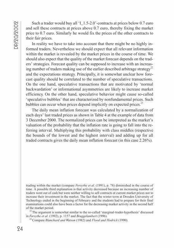
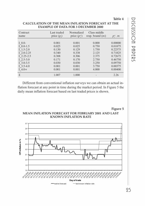
The daily mean inflation forecast was calculated by a normalization ofeach days’ last traded prices as shown in Table 4 at the example of data from3 December 2000. The normalized prices can be interpreted as the market’svaluation of the probability that the inflation rate is going to fall into the re-ferring interval. Multiplying this probability with class middles (respectivethe bounds of the lowest and the highest interval) and adding up for alltraded contracts gives the daily mean inflation forecast (in this case 2.26%).
trading within the market (compare Forsythe et al. (1991), p. 78) diminished in the course oftime. A possible third explanation is that activity decreased because an increasing number oftraders went out of cash but were neither willing to sell contracts at current market prices nor toincrease their investment in the market. The fact that the winter term at Dresden University ofTechnology ended in the beginning of February and the students had to prepare for their finalexaminations could also have been a factor for the decreasing market activity in the second halfof the market period.
22 The argument is somewhat similar to the so-called ‘marginal-trader-hypothesis’ discussedin Forsythe et al. (1992), p. 1157 and Bruggelambert (1996).
23 Compare Blanchard and Watson (1982) and Flood and Hodrick (1990).
25
Disc
ussion P
aper
sTable 4
CALCULATION OF THE MEAN INFLATION FORECAST AT THEEXAMPLE OF DATA FOR 3 DECEMBER 2000
Contract Last traded Normalized Class middlename price (pt) price (pt
n) resp. bound (m) ptn . m
I_0.0- 0.001 0.001 0.000 0.00000I_0.0-1.5 0.025 0.025 0.750 0.01875I_1.5-2.0 0.130 0.129 1.750 0.22575I_2.0-2.25 0.340 0.338 2.125 0.71825I_2.25-2.5 0.308 0.306 2.375 0.72675I_2.5-3.0 0.171 0.170 2.750 0.46750I_3.0-3.5 0.030 0.030 3.250 0.09750I_3.5-4.0 0.001 0.001 3.750 0.00375I_4.0+ 0.001 0.001 4.000 0.00400
Σ 1.007 1.000 - 2.26
Different from conventional inflation surveys we can obtain an actual in-flation forecast at any point in time during the market period. In Figure 5 thedaily mean inflation forecast based on last traded prices is shown.
Figure 5MEAN INFLATION FORECAST FOR FEBRUARY 2001 AND LAST
KNOWN INFLATION RATE
1.8
1.9
2.0
2.1
2.2
2.3
2.4
2.5
2.6
2.7
25.10.2
000
29.10.2
000
02.11.2
000
06.11.2
000
10.11.2
000
14.11.2
000
18.11.2
000
22.11.2
000
26.11.2
000
30.11.2
000
04.12.2
000
08.12.2
000
12.12.2
000
16.12.2
000
20.12.2
000
24.12.2
000
28.12.2
000
01.01.2
001
05.01.2
001
09.01.2
001
13.01.2
001
17.01.2
001
21.01.2
001
25.01.2
001
29.01.2
001
02.02.2
001
06.02.2
001
10.02.2
001
14.02.2
001
18.02.2
001
22.02.2
001
26.02.2
001
02.03.2
001
06.03.2
001
10.03.2
001
14.03.2
001
Day of trade
CP
I in
flatio
n in
%
mark et forec ast last known inflation rate
26
dp/
20/2
002 The mean inflation forecast was in between 2.0 and 2.5% within the
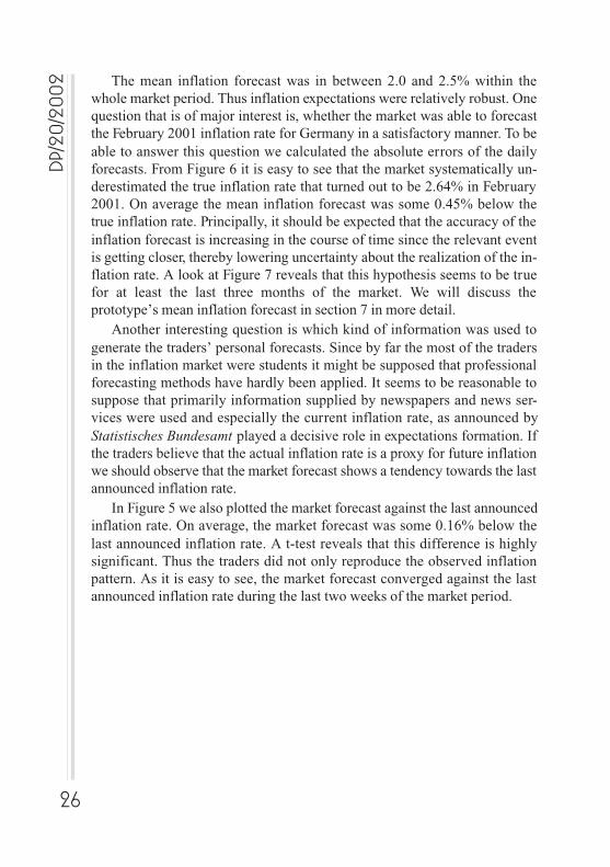
whole market period. Thus inflation expectations were relatively robust. Onequestion that is of major interest is, whether the market was able to forecastthe February 2001 inflation rate for Germany in a satisfactory manner. To beable to answer this question we calculated the absolute errors of the dailyforecasts. From Figure 6 it is easy to see that the market systematically un-derestimated the true inflation rate that turned out to be 2.64% in February2001. On average the mean inflation forecast was some 0.45% below thetrue inflation rate. Principally, it should be expected that the accuracy of theinflation forecast is increasing in the course of time since the relevant eventis getting closer, thereby lowering uncertainty about the realization of the in-flation rate. A look at Figure 7 reveals that this hypothesis seems to be truefor at least the last three months of the market. We will discuss theprototype’s mean inflation forecast in section 7 in more detail.
Another interesting question is which kind of information was used togenerate the traders’ personal forecasts. Since by far the most of the tradersin the inflation market were students it might be supposed that professionalforecasting methods have hardly been applied. It seems to be reasonable tosuppose that primarily information supplied by newspapers and news ser-vices were used and especially the current inflation rate, as announced byStatistisches Bundesamt played a decisive role in expectations formation. Ifthe traders believe that the actual inflation rate is a proxy for future inflationwe should observe that the market forecast shows a tendency towards the lastannounced inflation rate.
In Figure 5 we also plotted the market forecast against the last announcedinflation rate. On average, the market forecast was some 0.16% below thelast announced inflation rate. A t-test reveals that this difference is highlysignificant. Thus the traders did not only reproduce the observed inflationpattern. As it is easy to see, the market forecast converged against the lastannounced inflation rate during the last two weeks of the market period.
27
Disc
ussion P
aper
s
Figure 7AVERAGE MONTHLY PREDICTION ERRORS
Figure 6ABSOLUTE PREDICTION ERRORS OF DAILY MEAN
INFLATION FORECASTS
-0.9
-0.7
-0.5
-0.3
-0.1
0.1
0.3
0.5
0.7
25.10.2
000
30.10.2
000
04.11.2
000
09.11.2
000
14.11.2
000
19.11.2
000
24.11.2
000
29.11.2
000
04.12.2
000
09.12.2
000
14.12.2
000
19.12.2
000
24.12.2
000
29.12.2
000
03.01.2
001
08.01.2
001
13.01.2
001
18.01.2
001
23.01.2
001
28.01.2
001
02.02.2
001
07.02.2
001
12.02.2
001
17.02.2
001
22.02.2
001
27.02.2
001
04.03.2
001
09.03.2
001
14.03.2
001
Day of trade
Ab
so
lute
err
or
-0.556
-0.358
-0.449
-0.552
-0.272
-0.481
-0.6
-0.5
-0.4
-0.3
-0.2
-0.1
0.0
October November December January February March
Month
Avera
ge f
ore
cast
err
or
28
dp/
20/2
002 Measuring Uncertainty of the Mean Inflation Forecast
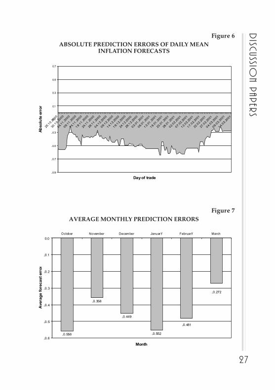
By far the most published inflation forecasts are mean forecasts. Typi-cally these forecasts do not provide any information on the underlying prob-abilities of different inflation scenarios that generated a certain forecast.Since a certain mean inflation forecast can result from different distributionsof individual predictions, information on the distribution of the forecast ishelpful in assessing the mean inflation forecast’s uncertainty.
In inflation expectation surveys, often the variance across the individualforecasts is used as a proxy for the uncertainty surrounding a mean inflationforecast. This is somewhat problematic since a high degree of dispersion inindividual forecasts might also be due to forecasters’ heterogeneous sets ofinformation. Thus using the variance as a proxy for the mean inflation fore-cast might be misleading.24
Figure 8VARIANCE OF DAILY MEAN INFLATION FORECAST
24 Bomberger (1996) showed at the example of U.S.-data for the period of 1946 up to 1994
that disagreement in the Livingston inflation expectation survey is correlated with uncertaintyderived by ARCH-models. Nevertheless it is at least controversial whether disagreement in in-flation expectation surveys is a useful proxy for uncertainty.
0.0
0.1
0.2
0.3
0.4
0.5
0.6
0.7
0.8
0.9
1.0
25.10.2
000
30.10.2
000
04.11.2
000
09.11.2
000
14.11.2
000
19.11.2
000
24.11.2
000
29.11.2
000
04.12.2
000
09.12.2
000
14.12.2
000
19.12.2
000
24.12.2
000
29.12.2
000
03.01.2
001
08.01.2
001
13.01.2
001
18.01.2
001
23.01.2
001
28.01.2
001
02.02.2
001
07.02.2
001
12.02.2
001
17.02.2
001
22.02.2
001
27.02.2
001
04.03.2
001
09.03.2
001
14.03.2
001
Day of trade
Vari
an
ce o
f in
flati
on
fo
recast
29
Disc
ussion P
aper
s
Our prototype market allows to assess the mean inflation forecast’s un-certainty directly. Since the normalized market prices pn
t,j can be interpreted
as the market’s aggregated evaluation of the probabilities of different infla-tion scenarios, these probabilities can be used to calculate the variance of thedaily mean inflation forecast as
2
1
,2
).( tj
J
j
njtt mt µ−=σ ∑
=
where J is the number of traded contract types, mj are the class middles (re-
spective bounds), µ is the mean inflation forecast and t is an index represent-ing time. The results are presented in Figure 8. We observe that the varianceof the daily mean inflation forecast in the prototype market decreasedsharply after a few days of trade and fluctuated around 0.25 thereafter.Within the last three months the variance showed a somewhat decreasingtendency thereby indicating a slightly diminishing degree of uncertainty.
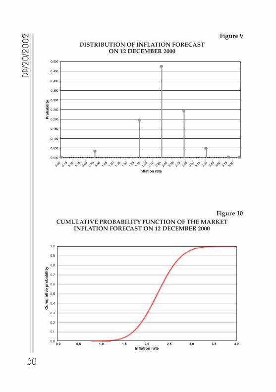
Normally Distributed Forecasts and Further ApplicationsFor each point in time during the market was open we can visualize the
market’s actual evaluation of the probability of different inflation realiza-tions in a histogram. In Figure 9 we show the empirical distribution of the in-flation forecast of 12 December 2000 (last traded prices). We have one ob-servation for each contract that is represented by its class middle (respectivethe class bound).
A first inspection of the histogram suggests that inflation expectationsmight be normally distributed. When extending the inspection to a largernumber of days at different points in time during the market period this sug-gestion is substantiated. Because of the relatively low number of observa-tions we are not able to test this hypothesis formally.
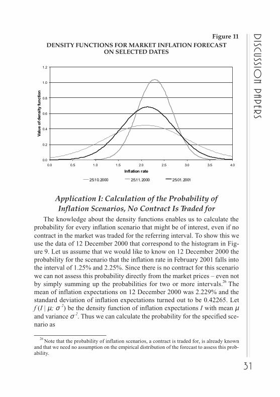
If in fact the market forecast is normally distributed – and that is what wewill assume in the following – we are able to make more precise statementsabout the probability of different inflation scenarios. Since we know themean and the standard deviation of the forecast we can calculate and graphthe cumulative probability function (compare the example of 12 December2000 that is shown in Figure 10). We can also calculate and graph the refer-ring density function. In Figure 11 we show the density functions on differ-ent days during the market period.25
25 Recently authors like Blix and Sellin (1999) and Wallis (1999) supposed inflation scenarios
often to be distributed asymmetrically. It should be noted that the market data also allow to cal-culate the moments of asymmetric distributions as e.g. the two-piece normal distribution.
30
dp/
20/2
002 Figure 9
DISTRIBUTION OF INFLATION FORECASTON 12 DECEMBER 2000
Figure 10CUMULATIVE PROBABILITY FUNCTION OF THE MARKET
INFLATION FORECAST ON 12 DECEMBER 2000
0.0 0.5 1.0 1.5 2.0 2.5 3.0 3.5 4.0
Inflation rate
1.0
0.9
0.8
0.7
0.6
0.5
0.4
0.3
0.2
0.1
0.0
Cu
mu
lati
ve p
rob
ab
ilit
y
0.000
0.050
0.100
0.150
0.200
0.250
0.300
0.350
0.400
0.450
0.500
0.00
0.15
0.30
0.45
0.60
0.75
0.90
1.05
1.20
1.35
1.50
1.65
1.80
1.95
2.10
2.25
2.40
2.55
2.70
2.85
3.00
3.15
3.30
3.45
3.60
3.75
3.90
Inflation rate
Pro
bab
ilit
y
31
Disc
ussion P
aper
s
26 Note that the probability of inflation scenarios, a contract is traded for, is already known
and that we need no assumption on the empirical distribution of the forecast to assess this prob-ability.
Application I: Calculation of the Probability ofInflation Scenarios, No Contract Is Traded for
The knowledge about the density functions enables us to calculate theprobability for every inflation scenario that might be of interest, even if nocontract in the market was traded for the referring interval. To show this weuse the data of 12 December 2000 that correspond to the histogram in Fig-ure 9. Let us assume that we would like to know on 12 December 2000 theprobability for the scenario that the inflation rate in February 2001 falls intothe interval of 1.25% and 2.25%. Since there is no contract for this scenariowe can not assess this probability directly from the market prices – even notby simply summing up the probabilities for two or more intervals.26 Themean of inflation expectations on 12 December 2000 was 2.229% and thestandard deviation of inflation expectations turned out to be 0.42265. Letf (I | µ; σ 2) be the density function of inflation expectations I with mean µand variance σ 2. Thus we can calculate the probability for the specified sce-nario as
Figure 11DENSITY FUNCTIONS FOR MARKET INFLATION FORECAST
ON SELECTED DATES
0.0
0.2
0.4
0.6
0.8
1.0
1.2
0.0 0.5 1.0 1.5 2.0 2.5 3.0 3.5 4.0
Inflation rate
Valu
e o
f d
en
sity fu
nctio
n
25.10.2000 25.11.2000 25.01.2001
32
dp/
20/2
002
Application II: Calculation of Confidence Intervalsand Modified Fan Charts
One might also be interested to calculate a confidence-interval for theFebruary inflation rate. Since we assumed a symmetric distribution, the con-fidence interval has to be symmetric around the mean of the distribution andcan be calculated quite easily. Let α be the confidence level we are interestedin. We know that the lower bound I
l of the confidence interval is the inflation
rate for which
( )2
5.0α−=∫
µdI If
É t
is fulfilled. Similarly the upper bound of the confidence interval Iu has to
fulfill the condition
( )2
5.0α
−=∫µdI If
É u .
Again we shall illustrate the argument by giving an example. We willtherefore assume that we are interested in the 95%-confidence interval forthe February inflation rate on the basis of the market data of 12 December2000. The upper bound is the 97.5%-quantile of the specified normal distri-bution:
Iu = 3.057%.
Since the distribution is symmetric the lower bound can easily be calcu-lated as
µ – (Iu – µ ) = 2 . µ – I
u = 1.401%.
Thus, the market judged the probability that the February inflation ratewill be in between 1.401% and 3.057% to be 0.95.
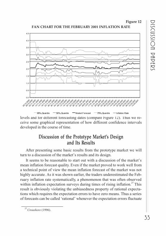
The Bank of England uses fan charts to present their inflation forecasts.These fan charts include a graphical representation of confidence intervalsfor inflation at different times in the future. Since our prototype market gen-erates a time series of forecasts for one certain future date only, we wouldneed several markets to reproduce such a fan chart. To produce a modifiedversion of a fan chart we calculate the confidence intervals for different α
5095.00103.05198.0..2
1
);|(25.225.1(
21
21 ).(25.2
25.1
25.2
25.1
2
=−≈πσ
=
=σµ=≤≤
σµ−−∫
∫dI
IfIp
e
33
Disc
ussion P
aper
s
27 Croushore (1996).
Figure 12FAN CHART FOR THE FEBRUARY 2001 INFLATION RATE
levels and for different forecasting dates (compare Figure 12). Thus we re-ceive some graphical representation of how different confidence intervalsdeveloped in the course of time.
Discussion of the Prototype Market’s Designand Its Results
After presenting some basic results from the prototype market we willturn to a discussion of the market’s results and its design.
It seems to be reasonable to start out with a discussion of the market’smean inflation forecast quality. Even if the market proved to work well froma technical point of view the mean inflation forecast of the market was nothighly accurate. As it was shown earlier, the traders underestimated the Feb-ruary inflation rate systematically, a phenomenon that was often observedwithin inflation expectation surveys during times of rising inflation.27 Thisresult is obviously violating the unbiasedness property of rational expecta-tions which requires the expectation errors to have zero means. Thus a seriesof forecasts can be called ‘rational’ whenever the expectation errors fluctuate
0.0
0.5
1.0
1.5
2.0
2.5
3.0
3.5
4.0
4.5
25.10.2
000
29.10.2
000
02.11.2
000
06.11.2
000
10.11.2
000
14.11.2
000
18.11.2
000
22.11.2
000
26.11.2
000
30.11.2
000
04.12.2
000
08.12.2
000
12.12.2
000
16.12.2
000
20.12.2
000
24.12.2
000
28.12.2
000
01.01.2
001
05.01.2
001
09.01.2
001
13.01.2
001
17.01.2
001
21.01.2
001
25.01.2
001
29.01.2
001
02.02.2
001
06.02.2
001
10.02.2
001
14.02.2
001
18.02.2
001
22.02.2
001
26.02.2
001
02.03.2
001
06.03.2
001
10.03.2
001
14.03.2
001
95%-Quantile 50%-Quantile Market Forecast 75%-Quantile Inflation Rate
34
dp/
20/2
002 around the true inflation rate. Even if it is desirable to have forecasts fulfill-
ing the properties of rational expectations we should note that most time se-ries of inflation forecasts are not satisfying these conditions.28 Thus the fail-ure to exhibit a ‘rational’ forecast pattern does not necessarily mean that aninflation market produces worse forecasting results than conventional fore-casting methods. To be able to judge whether electronic markets are a usefulmethod of forecasting macroeconomic variables more forecasting marketshave to be organized.
Nevertheless it seems to be reasonable to think about how to improve theforecasting quality of future inflation forecasting markets. As it was pointedout earlier it is very important that all important information on future infla-tion is present at least somewhere in the market. The fact that our prototypemarket included a relatively low number of 44 traders might be an explainingfactor for the low degree of accuracy of the market forecast. Possibly evenmore important is the fact that nearly all traders were students from two uni-versity courses. Since taking part in the market increased the probability ofpassing the courses’ final examinations (that also included questions on thefunctioning of electronic markets) at least some of the traders might have hadsomewhat disturbed incentives to take part. Therefore, the basic advantageof electronic markets to have traders only, who suppose to have superior in-formation on the event to be forecasted, was obviously not given in the pro-totype market. Thus it might be supposed that inflation market’s forecastingquality can be increased by advertising the market to a broader public audi-ence and especially not to run such a market as a mandatory part of an uni-versity course.
An important and still unresolved question is what is the optimal numberof contract types that should be traded in the market. On the one hand, the ac-curacy of the market forecast obviously increases with an increasing numberof contract types traded. This is due to the fact that we use the class middlesto calculate the mean inflation forecast, thereby assuming that all possibleoutcomes in the interval are equally likely. The forecasting errors caused byusing this procedure can be supposed to decrease when using smaller inter-vals for the contracts. On the other hand, the traders’ problem of determiningthe fair prices for the contracts can be supposed to be positively correlated tothe number of traded contracts. Up to now there is little evidence whichnumber of contracts solves this trade-off in an optimal way. A good strategymight be to start out with a relatively low number of contracts and then to
28 Compare e.g. Gramlich (1983), Pearce (1979) and Laubscher and Schombee (1999), p. 10.
35
Disc
ussion P
aper
s
split those contracts which turn out to be traded for the highest prices to in-crease the forecast’s quality.
As it was pointed out earlier, electronic markets can be used to predictany future event that is measurable objectively. Nevertheless we should un-derline that electronic markets are better suited to short-run forecasts than tolong-run predictions. This is due to the fact that the markets cannot be liqui-dated before the event, the market is conducted on, has taken place. Techni-cally it is no problem to run a long-term forecast market. Such a forecast canbe obtained from a market that is run several years before the event of inter-est takes place. But it is obvious that it will be hard to get traders for such amarket because there is a long period of time between trading and the liqui-dation of the market.
With respect to political stock markets critics often argue that electronicmarkets are no independent instruments because the traders in the marketswould simply reproduce the latest polls’ results. Even if some studies founda significant influence of polls on contract prices in political stock markets(compare e.g. Bruggelambert (1997) or Beckmann and Werding (1996)), re-cent results indicate that traders in electronic markets do not simply repro-duce poll results (compare Berlemann and Schmidt (2001)). Nevertheless itis hard to judge whether the results of political stock markets would havebeen as accurate as they have been when no polling information would havebeen at hand. This is due to the fact that typically a large number of polls isconducted on the occasion of political elections. It is somewhat easier to con-duct electronic forecasting markets on macroeconomic variables, no ad-equate forecast is available for. Doing so might help to answer the questionwhether electronic markets are an independent forecasting instrument.
Summary and OutlookIn this paper we presented a new method to generate inflation forecasts
via electronic markets. At the example of results from a class room experi-ment we demonstrated how the market data of a well-defined electronic mar-ket can be used to forecast mean inflation as well as the probability of differ-ent inflation scenarios at low costs. The promising results from the prototypemarket make us believe that the electronic market instrument is a useful fore-casting device.
To learn more about the accuracy of electronic market forecasts a largenumber of markets has to be conducted. To get well informed traders and toobtain a high quality forecast it could be useful to advertise the markets viamedia partners as it often has been done in political stock markets (note that

36
dp/
20/2
002 it is not necessary to have a somewhat representative sample of traders).
Electronic markets could also be used as an instrument to aggregate profes-sional forecasters’ individual predictions in a more reasonable and objectivemanner than it is often done within conventional consensus forecasts.
Up to now most electronic markets were conducted in environmentswhere other forecasts on the market event were available. Thus it might beinteresting to set up markets in countries where no reliable forecasts of mac-roeconomic variables exist. Currently first attempts are being undertaken toinstall a regular forecasting system for inflation, unemployment and the ex-change rate in Bulgaria.
37
Disc
ussion P
aper
s
ReferencesBank of England (1999) Economic Models at the Bank of England, London.
Batchelor, R. A. (1986) Quantitative and Qualitative Measures of Inflation Ex-pectations. Bulletin of Economics and Statistics, 48(2), 99 – 120.
Beckmann, K., Werding, M. (1996) Passauer Wahlborse: Information Process-ing in a Political Market Experiment, Kyklos, 49, 171 – 204.
Berlemann, M., Schmidt, C. (2001) Predictive Accuracy of Political StockMarkets. Empirical Evidence from a European Perspective, Discussion Pa-per 57/2001, Sonderforschungsbereich 373: Quantification and Simulationof Economic Processes, Humboldt University, Berlin.
Blanchard, O. J., Watson, M. W. (1982) Bubbles, Rational Expectations andFinancial Markets. In: P. Wachtel (Ed.), Crises in the Economic and Finan-cial Structure, Lexington, 295 – 316.
Blix, M., Sellin, P. (1999) Inflation Forecasts with Uncertainty Intervals.Sveriges Riksbank Quarterly Review, 2, 12 – 28.
Bomberger, W. A. (1996) Disagreement as a Measure of Uncertainty, Journal ofMoney, Credit and Banking, 28(3), 381 – 392.
Brayton, F., Levin, A., Tryon, R., Williams, J. (1997) The Evolution ofMacromodels at the Federal Reserve Board, Carnegie-Rochester Confer-ence Series on Public Policy, 47, 43 – 81.
Bruggelambert, G. (1996) Marginal Traders und die Hayek-Hypothese:Erfahrungen mit einer computerisierten Borse, Okonomie und Gesellschaft,Jahrbuch, 13, 214 – 272.
Bruggelambert, G. (1997) Von Insidern, “marginal traders” und Glucksrittern:Zur Relevanz von Entscheidungsanomalien in politischen Borsen,Jahrbucher fur Nationalokonomie und Statistik, 216/1, 45 – 73.
Croushore, D. (1993) Introducing: The Survey of Professional Forecasters, Fed-eral Reserve Bank of Philadelphia Business Review, 3 – 13.
Croushore, D. (1996) Inflation Forecasts: How Good Are They? Federal Re-serve Bank of Philadelphia Business Review, 5/6.
Deacon, M., Derry, A. (1994) Estimating Market Interest Rate and Inflation Ex-pectations from the Prices of UK Government Bonds, Bank of EnglandQuarterly Bulletin, 34, 232 – 240.
Drew, A., Hunt, B. (1998) The Forecasting and Policy System: preparing eco-nomic projections. Discussion Paper G98/7, Reserve Bank of NewZealand.
38
dp/
20/2
002 Estrella, A., Mishkin, F. S. (1997) The Predictive Power of the Term Structure
of Interest Rates in Europe and the United States: Implications for the Eu-ropean Central Bank, European Economic Review, 41, 1375 – 1401.
Fischer, I. (1930) The Theory of Interest, Macmillan, London.
Flood, R. P., Hodrick, R. J. (1990) On Testing for Speculative Bubbles, Journalof Economic Perspectives, 4 (2), 85 – 101.
Forsythe, R., Nelson, F., Neumann, G. R., Wright, J. (1992) Anatomy of anExperimental Stock Market, American Economic Review, 82, 1142 – 1161.
Forsythe, R., Frank, M., Krishnamurthy, V., Ross, T. W. (1995) Using MarketPrices to Predict Election Results: the UBC Election Stock Market, Cana-dian Journal of Economics, 28, 770 – 793.
Foster, J., Gregory, M. (1977) Inflation Expectations: the Use of QualitativeSurvey Data, Applied Economics, 9, 319 – 329.
Goodhart, C. (2001) The Inflation Forecast, National Institute Economic Re-view, 175, 59 – 66.
Gramlich, E. M. (1983) Models of Inflation Expectations Formation, Journal ofMoney, Credit and Banking, 15, 155 – 173.
Jansson, P., Vredin, A. (2001) Forecast-based monetary policy in Sweden1992-1998: A View from Within, Working Paper No. 120, SwedishRiksbank.
Jochum, Chr., Kirchgassner, G. (1999) Hat die Zinsstruktur Aussagekraft furdie zukunftige Inflation in Deutschland? Kredit und Kapital, 4/99, 493 –519.
Laubscher, P., Schombee, A. (1999) Measuring Inflation Expectations – The In-ternational Experience, Bureau of Economic Research, University of Stel-lenbosch.
Mishkin, F. S. (1990) What does the term structure tell us about future inflation?Journal of Monetary Economics, 25, 77 – 95.
Mishkin, F. S. (1991) A multi-country study of the information in the termstructure about future inflation, Journal of International Money and Fi-nance, 19, 2 – 22.
Ortner, G., Stepan, A., Zechner, J. (1995) Political Stock Markets, Zeitschriftfür Betriebswirtschaft. Ergänzungsheft 4/95, 12 3– 136.
Pearce, D. K. (1979) Comparing Survey and Rational Measures of Expected In-flation, Journal of Money, Credit and Banking, 11, 447 – 456.
39
Disc
ussion P
aper
sPoloz, S., Rose, D., Tetlow, R. (1994) The Bank of Canada’s new Quarterly Pro-
jection Model (QPM): An Introduction, Bank of Canada Review, Autumn,23 – 38.
Ragan, Chr. (1995) Deriving Agents’ Inflation Forecasts from the Term Struc-ture of Interest Rates, Working Paper 95-1, Bank of Canada.
Reserve Bank of New Zealand (1997) The Forecasting and Policy System: anintroduction, Reserve Bank Bulletin, 60 (3), 225 – 235.
Roberts, J. M. (1998) Inflation expectations and the transmission of monetarypolicy, Washigton D. C.
Sill, K. (1999) Forecasts, Indicators, And Monetary Policy, Federal ReserveBank of Philadelphia Business Review, 5/6, 3 – 14.
Soderlind, P., Svensson, L. E. O. (1997) New Techniques to Extract Market Ex-pectations from Financial Instruments, Journal of Monetary Economics,40(2), 373 – 429.
Stock, J., Watson, M. (1999) Forecasting inflation, Journal of Monetary Eco-nomics, 44, 293 – 335.
Svensson, L. E. O. (1994) The simplest test of inflation target credibility, CEPRDiscussion Paper No. 940, London.
Svensson, L. E. O. (1997) Inflation Targeting: Some Extensions, ScandinavianJournal of Economics, 101(3), 337 – 361.
Taylor, H. (1992) The Livingston Surveys: A History of Hopes and Fears, Fed-eral Reserve Bank of Philadelphia Business Review.
Wallis, K. F. (1999) Asymmetric Density Forecasts of Inflation and the Bank ofEngland’s Fan Chart, National Institute Economic Review, 1, 106 – 112.
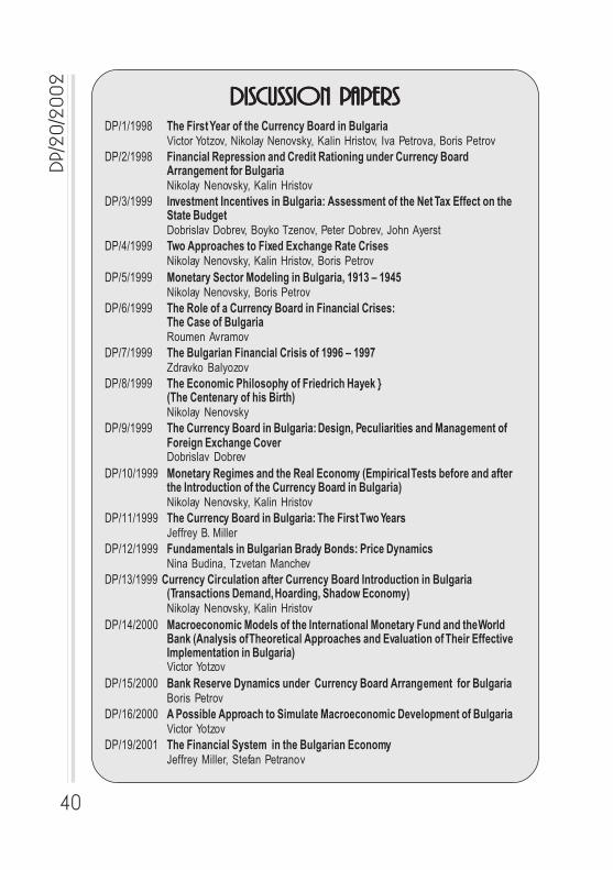
40
dp/
20/2
002
DISCUSSION PDISCUSSION PDISCUSSION PDISCUSSION PDISCUSSION PAPERSAPERSAPERSAPERSAPERSDP/1/1998 The First Year of the Currency Board in Bulgaria
Victor Yotzov, Nikolay Nenovsky, Kalin Hristov, Iva Petrova, Boris PetrovDP/2/1998 Financial Repression and Credit Rationing under Currency Board
Arrangement for BulgariaNikolay Nenovsky, Kalin Hristov
DP/3/1999 Investment Incentives in Bulgaria: Assessment of the Net Tax Effect on theState BudgetDobrislav Dobrev, Boyko Tzenov, Peter Dobrev, John Ayerst
DP/4/1999 Two Approaches to Fixed Exchange Rate CrisesNikolay Nenovsky, Kalin Hristov, Boris Petrov
DP/5/1999 Monetary Sector Modeling in Bulgaria, 1913 – 1945Nikolay Nenovsky, Boris Petrov
DP/6/1999 The Role of a Currency Board in Financial Crises:The Case of BulgariaRoumen Avramov
DP/7/1999 The Bulgarian Financial Crisis of 1996 – 1997Zdravko Balyozov
DP/8/1999 The Economic Philosophy of Friedrich Hayek }(The Centenary of his Birth)Nikolay Nenovsky
DP/9/1999 The Currency Board in Bulgaria: Design, Peculiarities and Management ofForeign Exchange CoverDobrislav Dobrev
DP/10/1999 Monetary Regimes and the Real Economy (Empirical Tests before and afterthe Introduction of the Currency Board in Bulgaria)Nikolay Nenovsky, Kalin Hristov
DP/11/1999 The Currency Board in Bulgaria: The First Two YearsJeffrey B. Miller
DP/12/1999 Fundamentals in Bulgarian Brady Bonds: Price DynamicsNina Budina, Tzvetan Manchev
DP/13/1999 Currency Circulation after Currency Board Introduction in Bulgaria(Transactions Demand, Hoarding, Shadow Economy)Nikolay Nenovsky, Kalin Hristov
DP/14/2000 Macroeconomic Models of the International Monetary Fund and the WorldBank (Analysis of Theoretical Approaches and Evaluation of Their EffectiveImplementation in Bulgaria)Victor Yotzov
DP/15/2000 Bank Reserve Dynamics under Currency Board Arrangement for BulgariaBoris Petrov
DP/16/2000 A Possible Approach to Simulate Macroeconomic Development of BulgariaVictor Yotzov
DP/19/2001 The Financial System in the Bulgarian EconomyJeffrey Miller, Stefan Petranov