Forecasting Guide Release A9 - Oracle · PDF fileJD Edwards World Forecasting Guide, Release...
156
JD Edwards World Forecasting Guide Release A9.3 E20706-02 April 2013
Transcript of Forecasting Guide Release A9 - Oracle · PDF fileJD Edwards World Forecasting Guide, Release...

JD Edwards WorldForecasting Guide
Release A9.3
E20706-02
April 2013

JD Edwards World Forecasting Guide, Release A9.3
E20706-02
Copyright © 2013, Oracle and/or its affiliates. All rights reserved.
This software and related documentation are provided under a license agreement containing restrictions on use and disclosure and are protected by intellectual property laws. Except as expressly permitted in your license agreement or allowed by law, you may not use, copy, reproduce, translate, broadcast, modify, license, transmit, distribute, exhibit, perform, publish, or display any part, in any form, or by any means. Reverse engineering, disassembly, or decompilation of this software, unless required by law for interoperability, is prohibited.
The information contained herein is subject to change without notice and is not warranted to be error-free. If you find any errors, please report them to us in writing.
If this is software or related documentation that is delivered to the U.S. Government or anyone licensing it on behalf of the U.S. Government, the following notice is applicable:
U.S. GOVERNMENT END USERS: Oracle programs, including any operating system, integrated software, any programs installed on the hardware, and/or documentation, delivered to U.S. Government end users are "commercial computer software" pursuant to the applicable Federal Acquisition Regulation and agency-specific supplemental regulations. As such, use, duplication, disclosure, modification, and adaptation of the programs, including any operating system, integrated software, any programs installed on the hardware, and/or documentation, shall be subject to license terms and license restrictions applicable to the programs. No other rights are granted to the U.S. Government.
This software or hardware is developed for general use in a variety of information management applications. It is not developed or intended for use in any inherently dangerous applications, including applications that may create a risk of personal injury. If you use this software or hardware in dangerous applications, then you shall be responsible to take all appropriate fail-safe, backup, redundancy, and other measures to ensure its safe use. Oracle Corporation and its affiliates disclaim any liability for any damages caused by use of this software or hardware in dangerous applications.
Oracle and Java are registered trademarks of Oracle and/or its affiliates. Other names may be trademarks of their respective owners.
Intel and Intel Xeon are trademarks or registered trademarks of Intel Corporation. All SPARC trademarks are used under license and are trademarks or registered trademarks of SPARC International, Inc. AMD, Opteron, the AMD logo, and the AMD Opteron logo are trademarks or registered trademarks of Advanced Micro Devices. UNIX is a registered trademark of The Open Group.
This software or hardware and documentation may provide access to or information on content, products, and services from third parties. Oracle Corporation and its affiliates are not responsible for and expressly disclaim all warranties of any kind with respect to third-party content, products, and services. Oracle Corporation and its affiliates will not be responsible for any loss, costs, or damages incurred due to your access to or use of third-party content, products, or services.

iii
Contents
Preface ................................................................................................................................................................. ix
Audience....................................................................................................................................................... ixDocumentation Accessibility ..................................................................................................................... ixRelated Documents ..................................................................................................................................... ixConventions ................................................................................................................................................. ix
1 Overview to Forecasting
1.1 System Integration ..................................................................................................................... 1-21.2 Features ....................................................................................................................................... 1-41.2.1 Forecasting Levels and Methods ...................................................................................... 1-51.2.2 Demand Patterns ................................................................................................................ 1-81.2.3 Forecast Accuracy ............................................................................................................... 1-91.3 Forecast Considerations ......................................................................................................... 1-101.4 Forecasting Process ................................................................................................................. 1-101.5 Major Tables ............................................................................................................................. 1-121.6 Supporting Tables ................................................................................................................... 1-121.7 Menu Overview ...................................................................................................................... 1-121.7.1 Fast Path Commands ...................................................................................................... 1-13
Part I Detail Forecasts
2 Overview to Detail Forecasts
2.1 Objectives .................................................................................................................................... 2-12.2 About Detail Forecasts .............................................................................................................. 2-1
3 Setting Up Detail Forecasts
3.1 Setting Up Forecasting Supply and Demand Inclusion Rules ............................................ 3-13.1.1 Processing Options .............................................................................................................. 3-33.2 Setting Up Forecasting Fiscal Date Patterns ........................................................................... 3-33.2.1 What You Should Know About ........................................................................................ 3-33.2.2 To set up forecasting fiscal date patterns ........................................................................ 3-43.3 Setting Up the 52 Period Date Pattern .................................................................................... 3-53.4 Setting Up Forecast Types ........................................................................................................ 3-6

iv
4 Work with Sales Order History
4.1 Copying Sales Order History ................................................................................................... 4-14.1.1 Before You Begin ................................................................................................................. 4-24.1.2 Processing Options .............................................................................................................. 4-24.2 Reviewing and Revising Sales Order History ....................................................................... 4-24.2.1 Example: Reviewing and Revising Sales Order History ............................................... 4-2
5 Work with Detail Forecasts
5.1 Creating Detail Forecasts .......................................................................................................... 5-15.1.1 Processing Options .............................................................................................................. 5-25.2 Reviewing Detail Forecasts ...................................................................................................... 5-25.2.1 Processing Options .............................................................................................................. 5-45.3 Revising Detail Forecasts .......................................................................................................... 5-45.3.1 Processing Options .............................................................................................................. 5-7
Part II Summary Forecasts
6 Overview to Summary Forecasts
6.1 Objectives .................................................................................................................................... 6-16.2 About Summary Forecasts ....................................................................................................... 6-16.2.1 Comparing Summaries of Detail and Summary Forecasts .......................................... 6-26.2.2 Example: Company Hierarchy ......................................................................................... 6-2
7 Set Up Summary Forecasts
7.1 Defining Distribution Hierarchies ........................................................................................... 7-17.1.1 Example: Distribution Hierarchy for Company 100 ...................................................... 7-27.1.2 Before You Begin ................................................................................................................. 7-37.1.3 Processing Options .............................................................................................................. 7-57.2 Revising Address Book Records .............................................................................................. 7-57.2.1 Before You Begin ................................................................................................................. 7-57.3 Reviewing Business Unit Data ................................................................................................. 7-67.3.1 Before You Begin ................................................................................................................. 7-77.3.2 What You Should Know About ........................................................................................ 7-87.4 Reviewing Item Branch Records .............................................................................................. 7-8
8 Generate Summaries of Detail Forecasts
8.1 Generating Summaries of Detail Forecasts ............................................................................ 8-18.1.1 Before You Begin ................................................................................................................. 8-28.1.2 What You Should Know About ........................................................................................ 8-28.1.3 Processing Options .............................................................................................................. 8-2
9 Work with Summaries of Forecasts
9.1 Reviewing a Summary Forecast .............................................................................................. 9-19.2 Revising a Summary Forecast .................................................................................................. 9-39.2.1 Processing Options .............................................................................................................. 9-6

v
9.3 Revising Summary Forecasts Using Force Changes ............................................................. 9-69.3.1 Example: Using Force Changes ........................................................................................ 9-79.3.2 Before You Begin ................................................................................................................. 9-89.3.3 What You Should Know About ........................................................................................ 9-89.3.4 Processing Options .............................................................................................................. 9-8
Part III Aggregate Planning Forecasts
10 Overview to Aggregate Planning Forecasts
10.1 Objectives .................................................................................................................................. 10-110.2 About Aggregate Planning Forecasts ................................................................................... 10-1
11 Understand Summary Forecasts
11.1 About Summary Forecasts .................................................................................................... 11-111.1.1 Comparing Summaries of Detail and Summary Forecasts ....................................... 11-1
12 Work with Summary Sales Order History
12.1 Copying Summary Sales Order History .............................................................................. 12-112.1.1 Before You Begin .............................................................................................................. 12-312.1.2 Processing Options ........................................................................................................... 12-312.2 Reviewing and Revising Sales Order History .................................................................... 12-312.2.1 Before You Begin .............................................................................................................. 12-312.2.2 Processing Options ........................................................................................................... 12-6
13 Generate Summary Forecasts
13.1 Generating Summary Forecasts ............................................................................................ 13-113.1.1 Before You Begin .............................................................................................................. 13-213.1.2 Processing Options ........................................................................................................... 13-2
14 Understand Planning Bill Forecasts
14.1 About Planning Bill Forecasts ................................................................................................ 14-114.1.1 Example: Pseudo Parent Item ........................................................................................ 14-114.2 Exploding the Forecast to the Item Level ............................................................................ 14-214.2.1 Example: Exploding the Forecast .................................................................................. 14-3
15 Set Up a Planning Bill
15.1 Setting Up Item Master Information .................................................................................... 15-115.1.1 Processing Options ........................................................................................................... 15-415.2 Entering Planning Bills ........................................................................................................... 15-515.2.1 Processing Options ........................................................................................................... 15-8
16 Generate Planning Bill Forecasts
16.1 Generating Planning Bill Forecasts ...................................................................................... 16-116.1.1 Before You Begin .............................................................................................................. 16-1

vi
16.1.2 Processing Options ........................................................................................................... 16-1
Part IV Processing Options
17 Detail Forecasts Processing Options
17.1 Supply/Demand Inclusion Rules (P34004).......................................................................... 17-117.2 Extract Sales Order History (P3465) ...................................................................................... 17-117.3 Forecast Generation (P34650) ................................................................................................. 17-217.4 Forecast Review (P34201) ....................................................................................................... 17-517.5 Forecast Revisions (P3460)...................................................................................................... 17-5
18 Summary Forecasts Processing Options
18.1 Summary Constants (P4091) .................................................................................................. 18-118.2 Forecast Generation (P34650) ................................................................................................. 18-118.3 Forecast Summary (P34600) ................................................................................................... 18-418.4 Forecast Summary Inquiry (P34200) ..................................................................................... 18-418.5 Forecast Forcing (P34610)....................................................................................................... 18-4
19 Aggregate Planning Forecasts Processing Options
19.1 Extract Sales Order History (P3465) ...................................................................................... 19-119.2 Forecast Summary Inquiry (P34200) ..................................................................................... 19-219.3 Summary Forecast Generation (P34640) ............................................................................. 19-319.4 Item Master Revisions (P4101) ............................................................................................. 19-519.5 Bill of Material Revisions (P3002) .......................................................................................... 19-619.6 Master Planning Schedule - Plant Maintenance (P3482).................................................... 19-7
A Forecast Calculation Examples
A.1 Forecast Calculation Methods.................................................................................................. A-1A.2 Forecast Performance Evaluation Criteria ............................................................................. A-2A.3 Method 1 - Specified Percent Over Last Year ........................................................................ A-2A.3.1 Forecast Calculation ........................................................................................................... A-2A.3.2 Simulated Forecast Calculation ........................................................................................ A-2A.3.3 Percent of Accuracy Calculation....................................................................................... A-3A.3.4 Mean Absolute Deviation Calculation ............................................................................ A-3A.4 Method 2 - Calculated Percent Over Last Year ..................................................................... A-3A.4.1 Forecast Calculation ........................................................................................................... A-3A.4.2 Simulated Forecast Calculation ........................................................................................ A-4A.4.3 Percent of Accuracy Calculation....................................................................................... A-4A.4.4 Mean Absolute Deviation Calculation ............................................................................ A-4A.5 Method 3 - Last year to This Year............................................................................................ A-4A.5.1 Forecast Calculation ........................................................................................................... A-4A.5.2 Simulated Forecast Calculation ........................................................................................ A-5A.5.3 Percent of Accuracy Calculation....................................................................................... A-5A.5.4 Mean Absolute Deviation Calculation ............................................................................ A-5A.6 Method 4 - Moving Average .................................................................................................... A-5A.6.1 Forecast Calculation ........................................................................................................... A-5

vii
A.6.2 Simulated Forecast Calculation ........................................................................................ A-6A.6.3 Percent of Accuracy Calculation....................................................................................... A-6A.6.4 Mean Absolute Deviation Calculation ............................................................................ A-6A.7 Method 5 - Linear Approximation .......................................................................................... A-6A.7.1 Forecast Calculation ........................................................................................................... A-6A.7.2 Simulated Forecast Calculation ........................................................................................ A-7A.7.3 Percent of Accuracy Calculation....................................................................................... A-7A.7.4 Mean Absolute Deviation Calculation ............................................................................ A-7A.8 Method 6 - Least Square Regression ....................................................................................... A-7A.8.1 Forecast Calculation ........................................................................................................... A-8A.8.2 Simulated Forecast Calculation ........................................................................................ A-8A.8.3 Percent of Accuracy Calculation....................................................................................... A-9A.8.4 Mean Absolute Deviation Calculation ............................................................................ A-9A.9 Method 7 - Second Degree Approximation ........................................................................... A-9A.9.1 Forecast Calculation ......................................................................................................... A-10A.9.2 Simulated Forecast Calculation ...................................................................................... A-11A.9.3 Percent of Accuracy Calculation..................................................................................... A-11A.9.4 Mean Absolute Deviation Calculation .......................................................................... A-11A.10 Method 8 - Flexible Method ................................................................................................... A-11A.10.1 Forecast Calculation ......................................................................................................... A-12A.10.2 Simulated Forecast Calculation ...................................................................................... A-12A.10.3 Percent of Accuracy Calculation..................................................................................... A-12A.10.4 Mean Absolute Deviation Calculation .......................................................................... A-12A.11 Method 9 - Weighted Moving Average................................................................................ A-12A.11.1 Forecast Calculation ......................................................................................................... A-13A.11.2 Simulated Forecast Calculation ...................................................................................... A-14A.11.3 Percent of Accuracy Calculation..................................................................................... A-14A.11.4 Mean Absolute Deviation Calculation .......................................................................... A-14A.12 Method 10 - Linear Smoothing .............................................................................................. A-14A.12.1 Forecast Calculation ......................................................................................................... A-15A.12.2 Simulated Forecast Calculation ...................................................................................... A-15A.12.3 Percent of Accuracy Calculation..................................................................................... A-15A.12.4 Mean Absolute Deviation Calculation .......................................................................... A-15A.13 Method 11 - Exponential Smoothing..................................................................................... A-15A.13.1 Forecast Calculation ......................................................................................................... A-16A.13.2 Simulated Forecast Calculation ...................................................................................... A-16A.13.3 Percent of Accuracy Calculation..................................................................................... A-17A.13.4 Mean Absolute Deviation Calculation .......................................................................... A-17A.14 Method 12 - Exponential Smoothing with Trend and Seasonality................................... A-17A.14.1 Forecast Calculation ......................................................................................................... A-17A.14.2 Forecast Calculation ......................................................................................................... A-19A.14.3 Simulated Forecast Calculation ...................................................................................... A-20A.14.4 Percent of Accuracy Calculation..................................................................................... A-20A.14.5 Mean Absolute Deviation Calculation .......................................................................... A-20A.15 Evaluating the Forecasts ......................................................................................................... A-20A.16 Mean Absolute Deviation (MAD) ......................................................................................... A-21A.16.1 Percent of Accuracy (POA).............................................................................................. A-21

viii
B Functional Servers
B.1 About Functional Servers ......................................................................................................... B-1
Index

ix
Preface
Welcome to the JD Edwards World Forecasting Guide.
AudienceThis document is intended for implementers and end users of JD Edwards World Forecasting system.
Documentation AccessibilityFor information about Oracle's commitment to accessibility, visit the Oracle Accessibility Program website at http://www.oracle.com/pls/topic/lookup?ctx=acc&id=docacc.
Access to Oracle SupportOracle customers have access to electronic support through My Oracle Support. For information, visit http://www.oracle.com/pls/topic/lookup?ctx=acc&id=info or visit http://www.oracle.com/pls/topic/lookup?ctx=acc&id=trs if you are hearing impaired.
Related DocumentsYou can access related documents from the JD Edwards World Release Documentation Overview pages on My Oracle Support. Access the main documentation overview page by searching for the document ID, which is 1362397.1, or by using this link:
https://support.oracle.com/CSP/main/article?cmd=show&type=NOT&id=1362397.1
ConventionsThe following text conventions are used in this document:
Convention Meaning
boldface Boldface type indicates graphical user interface elements associated with an action, or terms defined in text or the glossary.
italic Italic type indicates book titles, emphasis, or placeholder variables for which you supply particular values.
monospace Monospace type indicates commands within a paragraph, URLs, code in examples, text that appears on the screen, or text that you enter.

x

1
Overview to Forecasting 1-1
1Overview to Forecasting
This chapter contains these topics:
■ Section 1.1, "System Integration,"
■ Section 1.2, "Features,"
■ Section 1.3, "Forecast Considerations,"
■ Section 1.4, "Forecasting Process,"
■ Section 1.5, "Major Tables,"
■ Section 1.6, "Supporting Tables,"
■ Section 1.7, "Menu Overview."
Effective management of distribution and manufacturing activities begins with understanding and anticipating the needs of the market. Implementing a forecasting system allows you to quickly assess current market trends and sales so that you can make informed decisions about your company.
Forecasting is the process of projecting past sales demand into the future. An accurate forecast helps you make operations decisions. For this reason, forecasting should be a central activity in your operations. You can use forecasts to make planning decisions about:
■ Customer orders
■ Inventory
■ Delivery of goods
■ Work load
■ Capacity requirements
■ · Warehouse space
■ · Labor
■ · Equipment
■ Budgets
■ Development of new products
■ Workforce requirements
The Forecasting system can generate the following types of forecasts:
■ Detail forecasts - Detail forecasts are based on individual items.

System Integration
1-2 JD Edwards World Forecasting Guide
■ Summary forecasts - Summary (or aggregated) forecasts are based on larger groups, such as a product line.
■ Planning bill forecasts - Planning bill forecasts are based on groups of items in a bill of material format that reflect how an item is sold, not how it is built.
1.1 System Integration Forecasting is one of many systems that make up the Enterprise Requirements Planning and Execution (ERPx) system. Use the ERPx system to coordinate your inventory, raw material, and labor resources to deliver products according to a managed schedule. ERPx is fully integrated and ensures that information is current and accurate across your business operations. It is a closed-loop manufacturing system that formalizes the activities of company and operations planning, as well as the execution of those plans.
The following systems make up the JD Edwards World ERPx product group.

System Integration
Overview to Forecasting 1-3
Figure 1–1 Systems in the JD Edwards ERPxE Product Group
The Forecasting system generates demand projections that you use as input for JD Edwards World planning and scheduling systems. These systems calculate material requirements for all component levels, from raw materials to complex subassemblies.

Features
1-4 JD Edwards World Forecasting Guide
Figure 1–2 Forecasting System Diagram
The Resource Requirements Planning (RRP) system uses a forecast of future demand to estimate the time and resources needed to make a product.
The Master Production Schedule (MPS) system plans and schedules what a company expects to manufacture. Data from the Forecasting system is one MPS input that helps determine demand before you execute production plans.
Material Requirements Planning (MRP) is an ordering and scheduling system that explodes the requirements of all MPS parent items to the components. You can also use forecast data as demand input for lower-level MRP components that are service parts with independent demand (demand not directly or exclusively tied to production of a particular product at a particular branch or plant).
Distribution Requirements Planning (DRP) is a management system that plans and controls the distribution of finished goods. You can use forecasting data as input for DRP so you can more accurately plan the demand that you supply through distribution.
1.2 Features You can use the Forecasting system to:
■ Generate forecasts
■ Enter forecasts manually
■ Maintain both manually entered forecasts and forecasts generated by the system
■ Summarize the sales order history data in weekly or monthly time periods
■ Generate forecasts based on any or all of 12 different formulas that address a variety of forecast situations you might encounter
■ Calculate which of the 12 formulas provides the best fit forecast

Features
Overview to Forecasting 1-5
■ Define the hierarchy that the system uses to summarize sales order histories and detail forecasts
■ Create multiple hierarchies of address book category codes and item category codes, which you can use to sort and view records in the detail forecast table
■ Review and adjust both forecasts and sales order actuals at any level of the hierarchy
■ Integrate the detail forecast records into DRP, MPS, and MRP generations
■ Force changes made at any component level to both higher levels and lower levels
■ Set a bypass flag to prevent changes generated by the force program being made to a level
■ Store and display both original and adjusted quantities and amounts
■ Attach descriptive text to a forecast at the detail and summary levels
■ Forecast up to five years, based on the processing options settings
■ Import or export data
Flexibility is a key feature of the JD Edwards World Forecasting system. The most accurate forecasts take into account quantitative information, such as sales trends and past sales order history, as well as qualitative information, such as changes in trade laws, competition, and government. The system processes quantitative information and allows you to adjust it with qualitative information. When you aggregate, or summarize, forecasts, the system uses changes that you make at any level of the forecast to automatically update all other levels.
You can perform simulations based on the initial forecast, which allows you to compare different situations. After you accept a forecast, the system updates your manufacturing and distribution plan with any changes you have made.
1.2.1 Forecasting Levels and Methods You can generate both single-item (detail) forecasts and product line (summary) forecasts that reflect product demand patterns. Select from 12 forecasting methods, and the system analyzes past sales to calculate the forecast. The forecast includes detail information at the item level and higher-level information about a branch or the company as a whole.
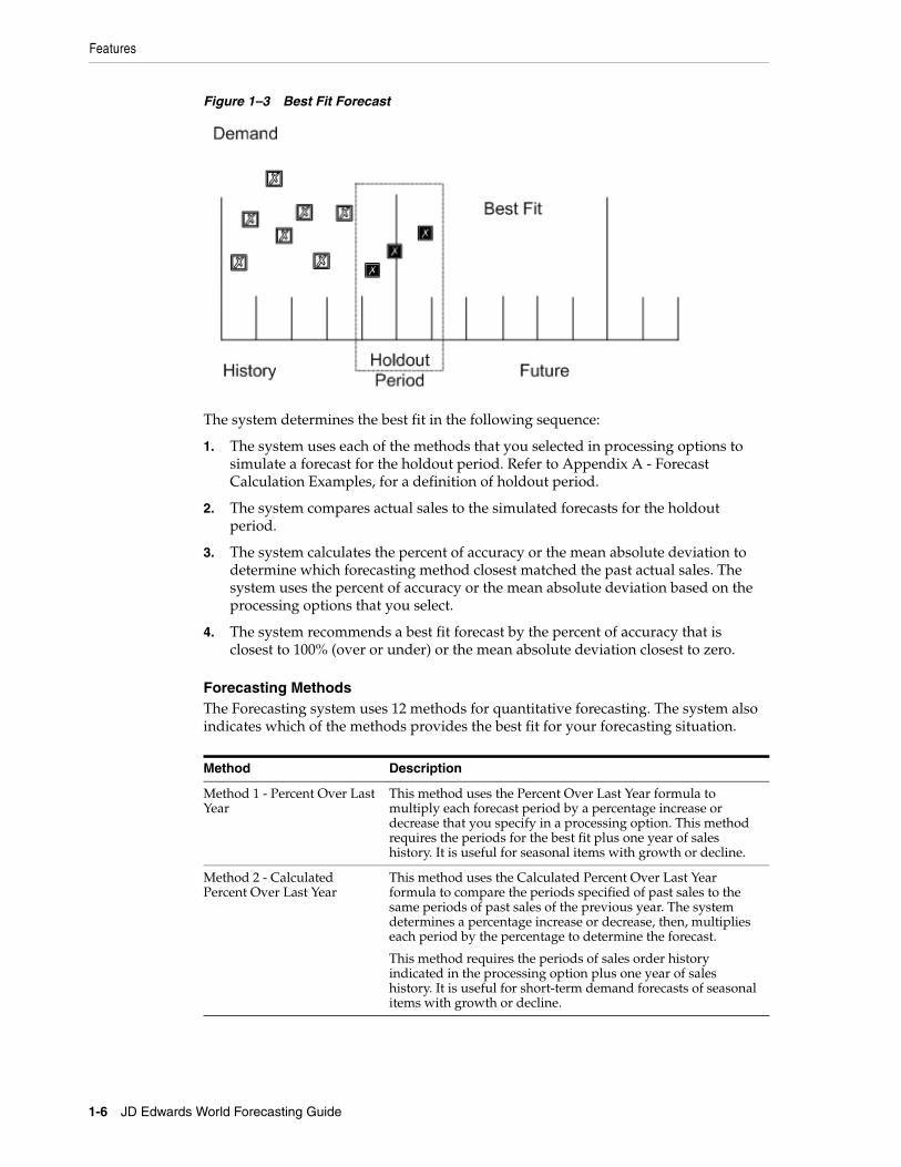
Best Fit The system recommends the best fit forecast by applying the selected forecasting methods to past sales order history and comparing the forecast simulation to the actual history. When you generate a forecast, the system compares actual sales order histories to forecasts for the months or weeks you indicate in the processing option and computes how accurately each of the selected forecasting methods would have predicted sales. Then, the system recommends the most accurate forecast as the best fit.
Features
1-6 JD Edwards World Forecasting Guide
Figure 1–3 Best Fit Forecast
The system determines the best fit in the following sequence:
1. The system uses each of the methods that you selected in processing options to simulate a forecast for the holdout period. Refer to Appendix A - Forecast Calculation Examples, for a definition of holdout period.
2. The system compares actual sales to the simulated forecasts for the holdout period.
3. The system calculates the percent of accuracy or the mean absolute deviation to determine which forecasting method closest matched the past actual sales. The system uses the percent of accuracy or the mean absolute deviation based on the processing options that you select.
4. The system recommends a best fit forecast by the percent of accuracy that is closest to 100% (over or under) or the mean absolute deviation closest to zero.
Forecasting Methods The Forecasting system uses 12 methods for quantitative forecasting. The system also indicates which of the methods provides the best fit for your forecasting situation.
Method Description
Method 1 - Percent Over Last Year
This method uses the Percent Over Last Year formula to multiply each forecast period by a percentage increase or decrease that you specify in a processing option. This method requires the periods for the best fit plus one year of sales history. It is useful for seasonal items with growth or decline.
Method 2 - Calculated Percent Over Last Year
This method uses the Calculated Percent Over Last Year formula to compare the periods specified of past sales to the same periods of past sales of the previous year. The system determines a percentage increase or decrease, then, multiplies each period by the percentage to determine the forecast.
This method requires the periods of sales order history indicated in the processing option plus one year of sales history. It is useful for short-term demand forecasts of seasonal items with growth or decline.

Features
Overview to Forecasting 1-7
Method 3 - Last Year to This Year
This method uses last year's sales for the following year's forecast. This method requires the periods best fit plus one year of sales order history. It is useful for mature products with level demand or seasonal demand without a trend.
Method 4 - Moving Average This method uses the Moving Average formula to average the months that you indicate in the processing option to project the next period. This method requires periods best fit from the processing option plus the number of periods of sales order history from the processing option. You should have the system recalculate it monthly or at least quarterly to reflect changing demand level. It is useful for mature products without a trend.
Method 5 - Linear Approximation
This method uses the Linear Approximation formula to compute a trend from the periods of sales order history indicated in the processing options and projects this trend to the forecast. You should have the system recalculate the trend monthly to detect changes in trends.
This method requires periods best fit plus the number of periods that you indicate in the processing option of sales order history. It is useful for new products or products with consistent positive or negative trends that are not due to seasonal fluctuations.
Method 6 - Least Square Regression (LSR)
This method derives an equation describing a straight line relationship between the historical sales data and the passage of time. LSR fits a line to the selected range of data such that the sum of the squares of the differences between the actual sales data points and the regression line are minimized. The forecast is a projection of this straight line into the future.
This method is useful when there is a linear trend in the data. It requires sales data history for the period represented by the number of periods best fit plus the number of historical data periods specified in the processing options. The minimum requirement is two historical data points.
Method 7 - Second Degree Approximation
This method uses the Second Degree Approximation formula to plot a curve based on the number of periods of sales history indicated in the processing options to project the forecast. This method requires periods best fit plus the number of periods indicated in the processing option of sales order history times three. It is not useful for long-term forecasts.
Method 8 - Flexible Method (Percent Over n Months Prior)
This method allows you to select the periods best fit block of sales order history starting n months prior and a percentage increase or decrease with which to modify it. This method is similar to Method 1, Percent Over Last Year, except that you can specify the number of periods that you use as the base.
Depending on what you select as n, this method requires months best fit plus the number of periods indicated in the processing options of sales data. It is useful for a planned trend.
Method Description

Features
1-8 JD Edwards World Forecasting Guide
1.2.2 Demand Patterns The Forecasting system uses sales order history to predict future demand. Different examples of demand follow. Forecast methods available in the JD Edwards World Forecasting system are tailored for these demand patterns.
Method 9 -
Weighted Moving Average
The Weighted Moving Average formula is similar to the Method 4, Moving Average formula, because it averages the previous number of months of sales history indicated in the processing options to project the next month's sales history. However, with this formula you can assign weights for each of the prior periods in a processing option.
This method requires the number of weighted periods selected plus months best fit data. Similar to Moving Average, this method lags demand trends, so it is not recommended for products with strong trends or seasonality. This method is useful for mature products with demand that is relatively level.
Method 10 -
Linear Smoothing
This method calculates a weighted average of past sales data. You can specify the number of periods of sales order history to use in the calculation (from 1 to 12) in a processing option. The system uses a mathematical progression to weigh data in the range from the first (least weight) to the final (most weight). Then, the system projects this information to each period in the forecast.
This method requires the months best fit plus the number of periods of sales order history from the processing option.
Method 11 -
Exponential Smoothing
This method uses one equation to calculate a smoothed average. This becomes an estimate representing the general level of sales over the selected historical range.
This method is useful when there is no linear trend in the data. It requires sales data history for the time period represented by the number of months best fit plus the number of historical data periods specified in the processing options. The minimum requirement is two historical data periods.
See Also:
■ Appendix A, "Forecast Calculation Examples."
Method Description

Features
Overview to Forecasting 1-9
Figure 1–4 Six Typical Demand Patterns
You can forecast the independent demand of the following items for which you have past data:
■ Samples
■ Promotional items
■ Customer orders
■ Service parts
■ Inter-plant demands
You can also forecast demand for the following item types determined by the manufacturing environments in which they are produced:
■ Make-to-stock - End items to meet customers' demand that occurs after the product is completed
■ Assemble-to-order - Subassemblies to meet customers' option selections
■ Make-to-order - Raw materials and components stocked in order to reduce lead time
1.2.3 Forecast Accuracy The following statistical laws govern the accuracy of a forecast:
■ A short-term forecast is more accurate than a long-term forecast, because the farther into the future you project the forecast, the more variables can impact the forecast.

Forecast Considerations
1-10 JD Edwards World Forecasting Guide
■ A forecast for a product family tends to be more accurate than a forecast for individual members of the product family. Some errors cancel as the forecasts for individual items summarize into the group.
1.3 Forecast Considerations You should not rely exclusively on past data to forecast future demands. The following circumstances might affect your business and require you to review and modify your forecast:
■ New products that have no past data
■ Plans for future sales promotion
■ Changes in national and international politics
■ New laws and government regulations
■ Weather changes and natural disasters
■ Innovations from competition
■ Economic changes
You might use any of the following kinds of long-term trend analysis to influence the design of your forecasts:
■ Market surveys
■ Leading economic indicators
■ Delphi panels
1.4 Forecasting Process You use Extract Sales Order History to copy data from the Sales History table (F42119) into either the Detail Forecast table (F3460) or possibly the Summary Forecast (F3400) table, depending on the kind of forecast you plan to generate.
You can generate detail forecasts or summaries of detail forecasts based on data in the Detail Forecast table. Data from your forecasts can then be revised. The process is illustrated in the following graphic.
The following graphic illustrates the sequences you follow when you use the detail forecasting programs.
See Also:
■ Appendix A, "Forecast Calculation Examples."

Forecasting Process
Overview to Forecasting 1-11
Figure 1–5 Detail Forecasts

Major Tables
1-12 JD Edwards World Forecasting Guide
1.5 Major Tables
1.6 Supporting Tables
1.7 Menu Overview JD Edwards World classifies the Forecasting system's menus according to frequency of use.
Table Description
Summary Forecast (F3400) Contains the summary forecasts generated by the system and the summarized sales order history created by the Extract Sales Order History program.
Detail Forecast (F3460) Contains the detail forecasts generated by the system and the sales order history created by the Extract Sales Actuals program.
Summary Constants (F4091) Stores the summary constants that you have set up for each product hierarchy.
Sales History (F42119) Contains past sales data, which provides the basis for the forecast calculations.
Sales Order Detail (F4211) Provides sales order demand by the requested date. The system uses this table to update the Sales History table for forecast calculations.
Table Description
Item Master (F4101) Stores basic information about each defined inventory item, such as item numbers, description, category codes, and units of measure.
Branch/Plant Master (F4102) Defines and maintains warehouse or plant level information, such as quantities, physical locations, and branch level category codes.
Business Unit Master (F0006) Identifies branch, plant, warehouse, or business unit information, such as company, description, and assigned category codes.
Address Book (F0101) Stores all address information pertaining to customers, vendors, employees, prospects, and other information.
Forecast Summary Work (F34006)
Ties the summary records (F3400) to the detail records (F3460).
Menu Overview
Overview to Forecasting 1-13
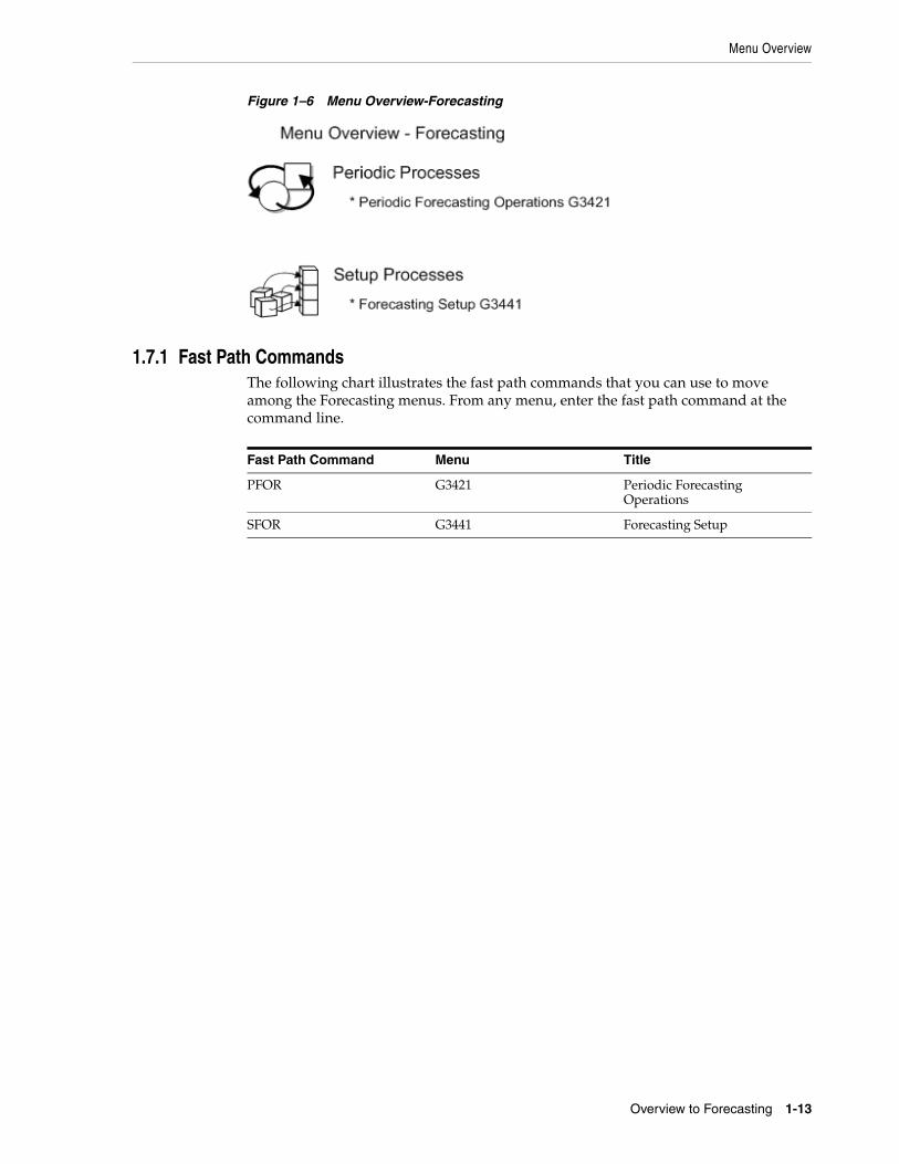
Figure 1–6 Menu Overview-Forecasting
1.7.1 Fast Path Commands The following chart illustrates the fast path commands that you can use to move among the Forecasting menus. From any menu, enter the fast path command at the command line.
Fast Path Command Menu Title
PFOR G3421 Periodic Forecasting Operations
SFOR G3441 Forecasting Setup

Menu Overview
1-14 JD Edwards World Forecasting Guide

Part IPart I Detail Forecasts
This part contains these chapters:
■ Chapter 2, "Overview to Detail Forecasts,"
■ Chapter 3, "Setting Up Detail Forecasts,"
■ Chapter 4, "Work with Sales Order History,"
■ Chapter 5, "Work with Detail Forecasts."


2
Overview to Detail Forecasts 2-1
2Overview to Detail Forecasts
This chapter contains these topics:
■ Section 2.1, "Objectives,"
■ Section 2.2, "About Detail Forecasts."
2.1 Objectives ■ To set up supply and demand inclusion rules
■ To set up fiscal date patterns
■ To set up a 52 period date pattern
■ To set up forecast types
■ To copy a sales order history into the Detail Forecast table
■ To review and revise a copied sales order history
■ To generate detail forecasts
■ To review detail forecasts
■ To revise detail forecasts
2.2 About Detail Forecasts You use detail forecasts to project demand at the single-item level according to each item's individual history.
Forecasts are based on sales data from the Sales Order History table (F42119), which is updated regularly with sales order demand information from the Sales Order Detail table (F4211). Before you generate forecasts, you use Extract Sales Order History to copy sales order history information from the Sales Order History table into the Detail Forecast table (F3460). This table also stores the generated forecasts.
Complete the following tasks:
■ Set up detail forecasts
■ Work with sales order history
■ Work with detail forecasts

About Detail Forecasts
2-2 JD Edwards World Forecasting Guide

3
Setting Up Detail Forecasts 3-1
3Setting Up Detail Forecasts
This chapter contains these topics:
■ Section 3.1, "Setting Up Forecasting Supply and Demand Inclusion Rules,"
■ Section 3.2, "Setting Up Forecasting Fiscal Date Patterns,"
■ Section 3.3, "Setting Up the 52 Period Date Pattern,"
■ Section 3.4, "Setting Up Forecast Types."
Before you generate a detail forecast, you set up criteria for the dates and kinds of data on which the forecasts will be based, as well as what time periods the system should use to structure the forecast output.
To set up detail forecasts, you must:
■ Set up inclusion rules to specify the sales history records on which you want to base the forecast
■ Specify beginning and end dates for the forecast
■ Indicate the date pattern on which you want to base the forecast
■ Add any forecast types not already provided by the system
3.1 Setting Up Forecasting Supply and Demand Inclusion Rules
NavigationFrom Material Planning Operations (G34), enter 29
From Material Planning Setup (G3440), choose Requirements Planning Setup
From Material Planning Setup (G3442), choose Supply/Demand Inclusion Rules
The Forecasting system uses supply and demand inclusion rules to determine which records from the Sales History table (F42119) to include or exclude when you run Extract Sales Order History. Supply and demand inclusion rules allow you to specify the status and type of items and documents to include in the records. You can set up as many different inclusion rule versions as you need for forecasting.
You should set up an inclusion rule for sales order records with status codes of 999 from the Sales History table.
To forecast by weeks, set up a 52 period calendar.

Setting Up Forecasting Supply and Demand Inclusion Rules
3-2 JD Edwards World Forecasting Guide
To set up supply and demand inclusion rules On Supply/Demand Inclusion Rules
Figure 3–1 Supply/Demand Inclusion Rules screen
1. Complete the following field:
■ Inclusion Code
2. Review the following fields:
■ Order Type
■ Line Type
■ Status Value
3. Select the lines that you want to include.
See Also:
■ Supply/Demand Inclusion Rules (P34004) in the JD Edwards World Manufacturing and Distribution Planning Guide.
■ Set Up 52 Period Accounting in the JD Edwards World General Accounting II Guide.
Field Explanation
Inclusion Code Identifies a group of items that the system can process together, such as reports, business units, or subledgers.
Or Ty Order Type

Setting Up Forecasting Fiscal Date Patterns
Setting Up Detail Forecasts 3-3
3.1.1 Processing OptionsSee Section 17.1, "Supply/Demand Inclusion Rules (P34004)."
3.2 Setting Up Forecasting Fiscal Date Patterns
NavigationFrom General Accounting (G09), choose Organization and Account Setup
From Organization and Account Setup (G09411), choose Company Numbers & Names
The Forecasting system uses fiscal date patterns to determine the time periods into which the sales order history is grouped. Before you can generate a detail forecast, set up a standard monthly date pattern. The system divides the sales history into weeks or months, depending on the processing option you have chosen. If you want to forecast by months, you must set up the fiscal date pattern. If you want to forecast by weeks, you must set up both the fiscal date pattern and a 52 period date pattern.
To set up fiscal date patterns, specify the beginning fiscal year, current fiscal period, and which date pattern to follow. The Forecasting system uses this information during data entry, updating, and reporting.
3.2.1 What You Should Know About
Ln Ty A code that controls how the system processes lines on a transaction. It controls the systems with which the transaction interfaces (General Ledger, Job Cost, Accounts Payable, Accounts Receivable, and Inventory Management). It also specifies the conditions under which a line prints on reports and is included in calculations. Codes include:
S – Stock item
J – Job cost
N – Non-stock item
F – Freight
T – Text information
M – Miscellaneous charges and credits
W – Work order
Sts Val A user defined code (system 40/type AT) that indicates the status of the line.
Topic Description
Controlling the date pattern JD Edwards World recommends you set up a separate fiscal date pattern for forecasting only, so you can control the date pattern. If you use the date pattern already established in the Financials system, the financial officer controls the date pattern.
Field Explanation

Setting Up Forecasting Fiscal Date Patterns
3-4 JD Edwards World Forecasting Guide
3.2.2 To set up forecasting fiscal date patterns On Company Numbers & Names
1. Access Date Pattern Revisions.
Figure 3–2 Company Numbers & Names screen
2. On Date Pattern Revisions, complete the following fields:
■ Fiscal Date Pattern Code
■ Fiscal Year Beginning Date
■ Fiscal Year Beginning Century
■ Date Pattern Type
■ End of Period Date
■ End of Period Century
Fiscal date pattern The fiscal date pattern must be an annual calendar. For example, January 1 through December 31.
Use the same date pattern for all forecasted items. A mix of date patterns across items that will be summarized at higher levels in the hierarchy causes unpredictable results.
Set up fiscal date patterns for as far back as your sales history extends, and as far forward as you want to forecast.
See Also:
■ Set Up 52 Period Accounting in the JD Edwards World General Accounting II Guide,
■ Set Up Fiscal Date Patterns in the JD Edwards World General Accounting I Guide.
Topic Description

Setting Up the 52 Period Date Pattern
Setting Up Detail Forecasts 3-5
3.3 Setting Up the 52 Period Date Pattern
NavigationFrom General Accounting (G09), enter 27
From G/L Advanced & Technical Operations (G0931), choose 52 Period Accounting
From 52 Period Accounting (G09313), choose Set 52 Period Dates
After you set up forecasting fiscal date patterns, you must set up a 52 period pattern for each code to forecast by weeks. When you set up a 52 period date pattern for a forecast, the period-ending dates are weekly instead of monthly.
To set up the 52 period date pattern On Set 52 Period Date
Field Explanation
Fiscal Date Pattern Code A code that identifies date patterns. You can use one of 15 codes. You must set up special codes (letters A through N) for 4-4-5, 13 period accounting, or any other date pattern unique to your environment. An R, the default, identifies a regular calendar pattern.
Fiscal Year Beginning - Date & Century
The first day of the fiscal year. A fiscal year spanning 1998 - 1999 and beginning September 1 would be entered as 090198 (US date format).
Date Pattern Type This field is used by Financial Analysis Spreadsheet Tool and Report Writer (FASTR) to determine the column headings that print on reports. It differentiates normal calendar patterns from 4-4-5 and 13 period accounting patterns. You can maintain headings for non-standard patterns in vocabulary override records R83360Mx, where x represents the value for this field.
End of Period 01 - Date & Century
The month end date in 12 period (monthly) accounting. The period end date in 13 period, 52 period, or 4-4-5 period accounting.
Form-specific information
You can use period 13 for audit adjustments in 12-period accounting by setting up period 12 to end on December 30 and period 13 to end on December 31. You can set up period 14 in the same way for 13 period or 4-4-5 accounting. The system validates the dates you enter.
See Also:
■ Set Up 52 Period Accounting in the JD Edwards World General Accounting II Guide.

Setting Up Forecast Types
3-6 JD Edwards World Forecasting Guide
Figure 3–3 Set Period 52 Dates screen
Complete the following fields:
■ Fiscal Date Pattern Code
■ Beginning of Fiscal Year
■ Beginning of Fiscal Year (Century)
■ Date Pattern Type
■ Period End Dates
■ Period End Centuries
3.4 Setting Up Forecast Types
NavigationFrom Periodic Forecasting Operations (G3421), enter 29
From Forecasting Setup (G3441), choose Forecast Types
You can add codes to the user defined code table (34/DF) that identifies forecast types, such as BF for Best Fit and AA for sales order history. The Forecasting system uses forecast type codes to determine which forecasting types to use when calculating a forecast. Processing options in DRP, MPS, and MRP allow you to enter forecast type codes to define which forecasting types to use in calculations. You can also use forecast type codes when you generate forecasts manually. Forecast Types 01 through 12 are hard-coded.
To set up forecast types On Forecast Types

Setting Up Forecast Types
Setting Up Detail Forecasts 3-7
Figure 3–4 Forecast Types screen
Complete the following fields:
■ Character Code
■ Description
Field Explanation
Character Code This column contains a list of valid codes for a specific user defined code list. The number of characters that a code can contain appears in the column title.
Description A user defined name or remark.

Setting Up Forecast Types
3-8 JD Edwards World Forecasting Guide

4
Work with Sales Order History 4-1
4Work with Sales Order History
This chapter contains these topics:
■ Section 4.1, "Copying Sales Order History,"
■ Section 4.2, "Reviewing and Revising Sales Order History."
The system generates detail forecasts based on sales history data that you copy from the Sales History table (F42119) into the Detail Forecast table (F3460). When you copy the sales history, you specify a date range based on the request date of the sales order. The demand history data can be distorted, however, by unusually large or small values (spikes or outliers), data entry errors, or lost sales (sales orders that were cancelled due to lack of inventory). You should review the data in the date range you specified to identify missing or inaccurate information. Then revise the sales order history to account for inconsistencies and distortions before you generate the forecast.
4.1 Copying Sales Order History
NavigationFrom Material Planning Operations (G34), choose Forecasting
From Periodic Forecasting Operations (G3421), choose Extract Sales Order History
The system generates detail and summary forecasts based on data in the Detail and/or Summary Forecast table. Use Extract Sales Order History to copy the sales order history (type AA) from the Sales History table to the Detail and/or Forecast table based upon criteria that you specify.
This program lets you:
■ Select a date range for the sales order history
■ Select a version of the inclusion rules to determine which sales history to include
■ Generate monthly or weekly sales order histories
■ Generate a separate sales order history for a large customer
■ Generate Summaries
■ Generate records with amounts, quantities, or both
You do not need to clear the Detail Forecast table before you run this program. The system automatically deletes any records that are:
■ For the same period as the actual sales order histories to be generated
■ For the same items

Reviewing and Revising Sales Order History
4-2 JD Edwards World Forecasting Guide
■ For the same sales order history type
■ For the same branch/plant
Records for Large Customers For your larger or more active customers, you can create separate forecasts and actual data. To define a customer as a large customer, you set up the customer as a type A customer in the ABC Code Sales field on Customer Master Information.
After you have set up the customer, set the appropriate processing option so that the system searches the sales history table for sales to that customer and creates separate Detail Forecast records for them.
If you have included customer level in the hierarchy the Sales Actuals with customers will summarize into separate branches of the hierarchy.
4.1.1 Before You Begin ■ Set up the detail forecast generation program. See Chapter 3, "Setting Up Detail
Forecasts."
■ Update sales order history. See Updating Customer Sales in the JD Edwards World Sales Order Management Guide.
4.1.2 Processing OptionsSee Section 19.1, "Extract Sales Order History (P3465)."
4.2 Reviewing and Revising Sales Order History
NavigationFrom Material Planning Operations (G34), choose Forecasting
From Periodic Forecasting Operations (G3421), choose Enter/Change Actuals
After you copy the sales order history into the Detail Forecast table, you should review the data for spikes, outliers, entry errors, or missing demand that might distort the forecast. You can then revise the sales order history manually to account for these inconsistencies before you generate the forecast.
Enter/Change Actuals allows you to create, change, or delete a sales order history manually. You can:
■ Review all entries in the Detail Forecast table
■ Revise the sales order history
■ Remove invalid sales history data, such as outliers or missing demand
4.2.1 Example: Reviewing and Revising Sales Order History In this example, you run Extract Sales Order History. The program identifies the actual quantities as shown in the following graphic.
See Also :
■ Update Sales Information in the JD Edwards World Sales Order Management Guide for more information on processes related to the daily updates of sales order history.

Reviewing and Revising Sales Order History
Work with Sales Order History 4-3
Figure 4–1 Enter Change Actuals screen
In the Quantity Adjusted field, the 775 value for 05/01/15 is an outlier. It could be a data entry error or a one-time demand that is unlikely to occur again. Use Enter/Change Actuals to revise the invalid outlier so you can generate an accurate forecast.
To review and revise sales order history On Enter/Change Actuals
Figure 4–2 Enter Change Actuals (Revise Sales Order History) screen
1. Complete the following fields:
■ Forecast Type
■ Item Number
■ Pass
■ Customer Number
The following field contains default information:

Reviewing and Revising Sales Order History
4-4 JD Edwards World Forecasting Guide
■ Unit of Measure
2. Review the following fields:
■ Request Date
■ Quantity Adjusted
■ Quantity Original
3. Access Amounts Adjusted.
4. On Amounts Adjusted, enter adjusted amounts.
5. Review the following field:
■ Amount Original
6. To access text window 0016, choose the Generic Text function.
7. Review the following fields for item information:
■ Item Number (short)
■ Business Unit
■ Forecast Type (Fc Ty)
8. To add descriptive information, complete the following field:
■ Text

5
Work with Detail Forecasts 5-1
5Work with Detail Forecasts
This chapter contains these topics:
■ Section 5.1, "Creating Detail Forecasts,"
■ Section 5.2, "Reviewing Detail Forecasts,"
■ Section 5.3, "Revising Detail Forecasts."
After you set up the actual sales history on which you plan to base your forecast, you generate the detail forecast. You can then revise the forecast to account for any market trends or strategies that might make future demand deviate significantly from the actual sales history.
This program also supports Import/Export functionality. See the JD Edwards World Technical Tools Guide for more information.
5.1 Creating Detail Forecasts
NavigationFrom Material Planning Operations (G34), choose Forecasting
From Periodic Forecasting Operations (G3421), choose Create Detail Forecast
The Create Detail Forecast program applies multiple forecasting methods to past sales histories and generates a forecast based on the method that is calculated to provide the most accurate prediction of future demand. The program can also calculate a forecast based on a selected method.
When you run Create Detail Forecast, the system:
■ Extracts sales order history information from the Detail Forecast table (F3460)
■ Calculates the forecasts using methods that you select
■ Calculates the percent of accuracy or the mean absolute deviation for each selected forecast method
■ Creates a simulated forecast for the months indicated in the processing option
■ Recommends the best fit forecast method
■ Creates the detail forecast in either dollars or units from the best fit forecast
■ Forecasts up to five years, as defined in the processing options
The system designates the extracted actual records as type AA and the best fit model as BF. Unlike forecast types 01 through 12, these forecast type codes are not hard-coded, so you can specify your own codes. The system stores both types of

Reviewing Detail Forecasts
5-2 JD Edwards World Forecasting Guide
records in the Detail Forecast table. The system does not automatically save the other forecast types 01 through 12 unless you set the processing options to do this.
You can also choose to include actual sales orders in your forecast by setting the appropriate processing options when you generate the forecast table. Including actual sales orders enables you to consider current sales activity in the forecasting process, which can enhance forecasting and planning accuracy.
This program allows you to:
■ Specify the number of months of actual data to use to create the best fit
■ Forecast for individual large customers for all methods
■ Run the forecast in proof or final mode
■ Create zero or negative forecasts, or both
■ Run the forecast simulation interactively
5.1.1 Processing OptionsSee Section 17.3, "Forecast Generation (P34650)."
5.2 Reviewing Detail Forecasts
NavigationFrom Material Planning Operations (G34), choose Forecasting
From Periodic Forecasting Operations (G3421), choose Review Forecast
You can display information by planner, master planning family, or both. You can then change the forecast type to compare different forecasts to the actual demand. You can also:
■ Display the data in summary or detail mode. The Detail mode lists all item numbers. The Summary mode consolidates data by master planning family.
■ Display all information stored in the Detail Forecast table.
■ Choose between quantities and amounts to review.
To review detail forecasts On Review Forecast

Reviewing Detail Forecasts
Work with Detail Forecasts 5-3
Figure 5–1 Review Forecast screen
1. Complete the following fields:
■ Year
■ Forecast Type
■ Branch/Plant
2. Complete one of the following fields:
■ Master Planning Family
■ Planner Number
3. Review the following fields:
■ Quantities Forecast
■ Quantities Sales Order History
■ Percent (%)
4. To access the amounts fields, choose Amounts/Quantities.
5. Review the following fields:
■ Amounts Forecast
■ Amounts Sales Order History
6. To display data in detail mode, choose the Detail selection on an item line.
Field Explanation
Year The calendar year.
Forecast Type A code from the user defined code table 34/DF that indicates either:
■ The forecasting method used to calculate the numbers displayed about the item
■ The actual historical information about the item

Revising Detail Forecasts
5-4 JD Edwards World Forecasting Guide
5.2.1 Processing OptionsSee Section 17.4, "Forecast Review (P34201)."
5.3 Revising Detail Forecasts
NavigationFrom Material Planning Operations (G34), choose Forecasting
From Periodic Forecasting Operations (G3421), choose Enter/Change Forecast
After you generate and review a forecast, you can revise the forecast to account for changes in consumer trends, market conditions, competitors' activities, your own marketing strategies, and so on. When you revise a forecast, you can:
■ Change information in an existing forecast manually
■ Add a forecast
■ Delete a forecast
Bch/Plt An alphanumeric field that identifies a separate entity within a business for which you want to track costs. For example, a business unit might be a warehouse location, job, project, work center, or branch/plant.
You can assign a business unit to a voucher, invoice, fixed asset, and so on, for purposes of responsibility reporting. For example, the system provides reports of open accounts payable and accounts receivable by business units to track equipment by responsible department.
Security for this field can prevent you from locating business units for which you have no authority.
Note: The system uses this value for Journal Entries if you do not enter a value in the AAI table.
Form-specific information
On this form, this is the branch/plant for which you review and revise a forecast.
Master Planning Family A code (table 41/P4) that represents an item property type or classification, such as commodity type, planning family, or so forth. The system uses this code to sort and process like items.
This field is one of six classification categories available primarily for purchasing purposes.
Planner Number The address number of the material planner for this item.
Form-specific information
You can use this field, along with the Master Planning Family and Year fields, to display specific forecast items. For example, you can show items within a planning family that were forecasted by a specific planner for a specific year.
Quantities Forecast The quantity of units affected by this transaction.
Form-specific information
The quantity of units in the sales order history on which a forecast is based.
Field Explanation

Revising Detail Forecasts
Work with Detail Forecasts 5-5
You can access forecasts that you want to revise by item number, branch plant, forecast type, or any combination of these elements. If your forecast is extensive, you can specify a beginning request date to limit the display.
As you revise the forecast, be aware that at least one of the following must be unique for each item number and branch record:
■ Forecast type
■ Request date
■ Customer number
For example, if two records have the same request date and customer number, they must have different forecast types.
To revise detail forecasts On Enter/Change Forecast
Figure 5–2 Enter/Change Forecast screen
1. To choose the forecast you want to revise, review the following fields:
■ Branch/Plant
■ Forecast Type
■ U/M (Unit of Measure) (Optional)
■ Item Number
2. Complete the following field:
■ Quantity Adjusted
3. To access amounts, choose Amounts/Quantities.
4. Revise the following field:
■ Amount Adjusted (F15)
5. To enter descriptive text, access Forecast Text.

Revising Detail Forecasts
5-6 JD Edwards World Forecasting Guide
Figure 5–3 Forecast Text screen
6. On Forecast Text, enter any descriptive text for the forecast.
Field Explanation
Bch/Plt An alphanumeric field that identifies a separate entity within a business for which you want to track costs. For example, a business unit might be a warehouse location, job, project, work center, or branch/plant.
You can assign a business unit to a voucher, invoice, fixed asset, and so on, for purposes of responsibility reporting. For example, the system provides reports of open accounts payable and accounts receivable by business units to track equipment by responsible department.
Security for this field can prevent you from locating business units for which you have no authority.
Note: The system uses this value for Journal Entries if you do not enter a value in the AAI table.
Form-specific information
On this form, this is the branch/plant for which you are reviewing and revising a sales order history or forecast.
Forecast Type A code from the user defined code table 34/DF that indicates either:
■ The forecasting method used to calculate the numbers displayed about the item
■ The actual historical information about the item
U/M A user defined code (00/UM) that indicates the quantity in which to express an inventory item, for example, CS (case) or BX (box).
Form-specific information
The Material Requirements Planning system converts this to the primary unit of measure for planning purposes.
Item Number A number that the system assigns to an item. It can be in short, long, or 3rd item number format.

Revising Detail Forecasts
Work with Detail Forecasts 5-7
5.3.1 Processing OptionsSee Section 17.5, "Forecast Revisions (P3460)."
Original The quantity of units affected by this transaction.
Form-specific information
The original quantity of units forecasted for production during a planning period.
Amount The current amount of the forecasted units for a planning period.
Field Explanation

Revising Detail Forecasts
5-8 JD Edwards World Forecasting Guide

Part IIPart II Summary Forecasts
This part contains these chapters:
■ Chapter 6, "Overview to Summary Forecasts,"
■ Chapter 7, "Set Up Summary Forecasts,"
■ Chapter 8, "Generate Summaries of Detail Forecasts,"
■ Chapter 9, "Work with Summaries of Forecasts."


6
Overview to Summary Forecasts 6-1
6Overview to Summary Forecasts
This chapter contains these topics:
■ Section 6.1, "Objectives,"
■ Section 6.2, "About Summary Forecasts."
6.1 Objectives ■ To define the distribution hierarchy
■ To revise address book records
■ To review branch or plant data
■ To review item branch records
■ To generate summaries of detail forecasts
■ To revise summaries of forecasts
■ To revise summaries of forecasts using the Force Changes program
6.2 About Summary Forecasts You use summary forecasts to project demand at a product group level. Summary forecasts are also called aggregate forecasts. You can generate a summary of a detail forecast based on detail sales histories or a summary forecast based on summary actual data.
The system updates the Sales History table (F42119) with sales data from the Sales Order table (F4211). You copy the sales history into the Summary Forecast table (F3400) to generate summary forecasts. You copy the sales history into the Detail Forecast table (F3460) to generate summaries of detail forecasts. The system generates summary forecasts that provide information for each level of the hierarchy that you set up with summary constants. These constants are stored in the Summary Constants table (F4091). Both summary forecasts and summaries of detail forecasts are stored in the Summary Forecast table.
Complete the following tasks:
■ Set up summary forecasts
■ Generate summaries of detail forecasts
■ Work with summaries of forecasts

About Summary Forecasts
6-2 JD Edwards World Forecasting Guide
6.2.1 Comparing Summaries of Detail and Summary Forecasts A summary of a detail forecast uses item-level data and predicts future sales in terms of both item quantities and sales amounts.
A summary forecast uses summary data to predict future sales.
6.2.2 Example: Company Hierarchy You need to define your company's hierarchy before you generate a summary forecast. JD Edwards World recommends that you organize the hierarchy by creating a diagram or storyboard. The following example illustrates this process.
■ Company 100 consists of two regions East (EST) and West (WST).
Figure 6–1 Company 100
■ Within the East Region, there are two sales territories, Southeastern (SOE) and Northeastern (NOE).
■ Within the West Region, there are two sales territories, Southwestern (SOW) and Northwestern (NOW).
Figure 6–2 Company 100 Regions
■ Each Sales Territory consists of two branch/plants:
■ SOE: B/P 30 (Memphis) and B/P 95 (Miami)
■ NOE: B/P 20 (Valley Forge) and B/P 80 (Boston)
■ SOW: B/P 10 (Modesto) and B/P 19 (Phoenix)
■ NOW: B/P 55 (Portland) and B/P 56 (Cheyenne)

About Summary Forecasts
Overview to Summary Forecasts 6-3
Figure 6–3 Company 100 East Region (EST)
Figure 6–4 Company 100 West Region (WEST)
Each branch or plant distributes hand tools (TLS), including hammers (HMR) and wrenches (WCH). The following item numbers represent the four main products.

About Summary Forecasts
6-4 JD Edwards World Forecasting Guide
Hierarchy of Company 100 The user defined hierarchy for Company 100 is:
■ 01 = Location field (for example, a region). Specified by category code 01 in the Address Book system.
■ 02 = Sales Territory. Specified by category code 03 in the Address Book system.
■ 03 = Purchasing Commodity Class. Specified by category code P1 in Branch/Plant.
Each item rolls up to an appropriate Purchasing Commodity Code. The lowest level is the sales order history or forecast for an item at the branch or plant level.
Summary Codes For each hierarchy you define, you must specify a unique identifier called a summary code. You can define for each summary code what each level of the hierarchy represents. Then, you can enter the summary code during summary forecasting programs to indicate which hierarchy you want to work with.
The following table illustrates a sample hierarchy defined for Company 100.
The sample data in the chart includes two sets of user defined codes. You can access the codes at the level that you choose. The location level (UDC 01/01) contains WST and EST.
Item Master Planning Family Commodity Class
2233 TLS WCH
2244 TLS WCH
5566 TLS HMR
5577 TLS HMR
Branch/Plant Region or Territory
Address Book Number Description Location Sales Territory
WST 100676 West Region
EST 100677 East Region
NOE 100678 Northeast EST
SOE 100680 Southeast EST
NOW 100679 Northwest WST
SOW 100681 Southwest WST
10 1063 Modesto WST SOW
19 100675 Phoenix WST SOW
20 1064 Valley Forge EST NOE
30 1062 Memphis EST SOE
55 100672 Portland WST NOW
56 100674 Cheyenne WST NOW
80 100669 Boston EST NOE
95 100671 Miami EST SOE

About Summary Forecasts
Overview to Summary Forecasts 6-5
The following sample screen illustrates codes set at the location level.
Figure 6–5 Forecast Types screen
The Sales Territory level (UDC 01/03) contains NOW, SOW, NOE, and SOE.
The following sample screen illustrates codes set at the sales territory level.
Figure 6–6 Forecast Types (Codes Set) screen
The Purchasing Commodity Class level (UDC 41/P1) contains HMR and WCH.
See Also :
■ Section 7.1, "Defining Distribution Hierarchies."

About Summary Forecasts
6-6 JD Edwards World Forecasting Guide

7
Set Up Summary Forecasts 7-1
7Set Up Summary Forecasts
This chapter contains these topics:
■ Section 7.1, "Defining Distribution Hierarchies,"
■ Section 7.2, "Revising Address Book Records,"
■ Section 7.3, "Reviewing Business Unit Data,"
■ Section 7.4, "Reviewing Item Branch Records."
In addition to the information set up for detail forecasts, the Forecasting system requires sales order history information to generate a summary forecast.
To set up summary forecasts, you must:
■ Define the hierarchy with codes and constants
■ Enter address book, branch or plant, and item branch data
Before You Begin ■ Set up detail forecasts. See Chapter 3, "Setting Up Detail Forecasts."
■ Create on paper a map or storyboard diagramming your definition of the company hierarchy. See Chapter 6, "Overview to Summary Forecasts."
7.1 Defining Distribution Hierarchies
NavigationFrom Material Planning Operations (G34), enter 29
From Material Planning Setup (G3440), choose Forecasting Setup
From Forecasting Setup (G3441), choose an option
The Forecasting system generates a summary forecast based on the distribution hierarchy that you define and select.
To define the distribution hierarchy, complete the following tasks:
■ Set up summary codes
■ Assign summary constants
You assign a summary code to each hierarchy that you define. For each summary code, you should identify the levels of the hierarchy. For each summary code, you can define up to 14 levels, as follows:

Defining Distribution Hierarchies
7-2 JD Edwards World Forecasting Guide
■ You can define the top level as the global summary level. You determine whether to summarize forecasts globally across multiple companies in the hierarchy at the global level.
■ You can define the next level as the company summary level. You determine whether to summarize forecasts for an entire company at the company summary level.
■ You can define up to 11 middle levels, which include the category codes and the customer level. You can choose from 20 address book category codes and 20 item balance category codes that you can assign to different levels in the hierarchy. The available codes all appear in the Summary Constants table. In the Customer Level field, you can specify what level of the hierarchy the customer number should be. This acts as another category code level.
■ You can define one bottom level. The lowest level you can define is the item level. In the Item Number field, you can indicate that the forecast should extend to the item level.
■ The branch or plant item detail records are automatically placed at the bottom level. The system does not include these as one of the 14 levels in the hierarchy.
7.1.1 Example: Distribution Hierarchy for Company 100 The following chart shows an example of a distribution hierarchy for the West Region of Company 100. The East Region section of the chart would extend to the right.
Figure 7–1 Example Distribution Hierarchy for Company 100’s West Region
In this example, you define the hierarchy for the West Region as follows:
1. Set up a West Region summary code WST.
You assign levels to in the Summary Constants table for summary code WST as follows:
1. Assign 01 to Location or Branch.
2. Assign 02 to Sales Territory.

Defining Distribution Hierarchies
Set Up Summary Forecasts 7-3
3. Assign 03 to Purchase Commodity Class.
4. Include the item in the hierarchy that will be the last level.
7.1.2 Before You Begin ■ Update the Sales history.
To set up summary codes You use the summary codes entered in the Character Code fields to define the summary hierarchy when you set up summary constants.
On Summary Codes
Figure 7–2 Forecast Types (Character Codes) screen
Complete the following fields:
■ Character Code - Summary Code
■ Description
To assign summary constants On Summary Constants
See Also:
■ See Update Sales Information in the JD Edwards World Sales Order Management Guide.
Field Explanation
Character Code This column contains a list of valid codes for a specific user defined code list. The number of characters that a code can contain appears in the column title.
Description A user defined name or remark.

Defining Distribution Hierarchies
7-4 JD Edwards World Forecasting Guide
Figure 7–3 Summary Constants screen
1. To display the sample summary constants, enter SUM in the following field:
■ Summary Code
2. Complete the following field (for your own code):
■ Summary Code
3. Complete the following fields:
■ Global Summary Y/N
■ Company Summary Y/N
■ Item Summary Y/N
■ Customer Level
4. To specify the hierarchy levels, complete Category Code fields.
Use the scroll keys to display and enter additional summary constants.
Figure 7–4 Summary Constants (Global Sum) screen

Revising Address Book Records
Set Up Summary Forecasts 7-5
7.1.3 Processing OptionsSee Section 18.1, "Summary Constants (P4091)."
7.2 Revising Address Book Records
NavigationFrom Master Directory (G), choose Address Book
From Address Book (G01), choose Address Book Revisions
After you have defined the company hierarchies, you need to revise the address book records so they include the new information.
When you generate a summary forecast and have address book category codes in the hierarchy, the system properly applies the forecast to the entire hierarchy only if you have assigned the appropriate code to each address in the address book.
For example, you have assigned a purchasing category code to an individual product belonging to a branch. If you have entered appropriate codes for each level of the hierarchy in the address book, the category code for the branch record links the individual product at the branch to a commodity class, which links to a sales territory, which links to a region, which links to the whole company.
To revise address book records, complete the following task:
■ Enter category codes (F14)
7.2.1 Before You Begin ■ Enter new records for all locations and customers defined in your distribution
hierarchy that are not included in your address book
Field Explanation
Summary Code The key to distinguish between different forecasting hierarchies.
Global Summary Y/N This flag indicates whether the forecast should be summarized to the global level. This level is the top level of the forecasting hierarchy and represents a summarization of all levels.
Company Summary Y/N This flag indicates whether the forecast should be summarized to the Company level. This level is the next level above the level indicated as number one in the hierarchy. All forecasts within the company will be summarized into this level.
Item Summary Y/N This flag indicates whether the forecast should be summarized down to the item number level. This level is the last level in the hierarchy. All forecast detail records for an item will be summarized into this level.
Customer Level To use Customer Number as one of the levels in the forecasting hierarchy, enter that level number here.
Item Category Codes Key Positions
An indicator that specifies which level in the forecasting hierarchy a specific Category Code should be.
See Also:
■ Enter Address Book Records in the JD Edwards World Address Book and Electronic Mail Guide.

Reviewing Business Unit Data
7-6 JD Edwards World Forecasting Guide
To enter category codes On Address Book Revisions
1. Choose Category Codes.
Figure 7–5 Category Codes screen
2. On Category Codes, complete the following fields:
■ Address Number
■ Category Codes
The following field contains default information:
■ Alpha Name
7.3 Reviewing Business Unit Data
NavigationFrom General Accounting (G09), choose Organization and Account Setup
From Organization and Account Setup (G09411), choose Business Units by Company
Field Explanation
Address Number A number that identifies an entry in the Address Book system. Use this number to identify employees, applicants, participants, customers, suppliers, tenants, and any other Address Book members.
Form-specific information
If you leave this field blank, the system assigns a number using the Next Numbers program.
Alpha Name The text that names or describes an address. This 40-character alphabetic field appears on a number of forms and reports. You can enter dashes, commas, and other special characters, but the system cannot search on them when you use this field to search for a name.
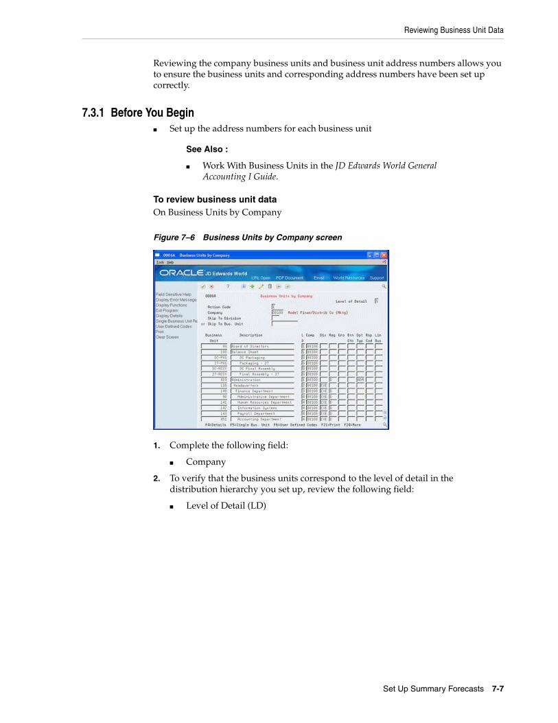
Reviewing Business Unit Data
Set Up Summary Forecasts 7-7
Reviewing the company business units and business unit address numbers allows you to ensure the business units and corresponding address numbers have been set up correctly.
7.3.1 Before You Begin ■ Set up the address numbers for each business unit
To review business unit data On Business Units by Company
Figure 7–6 Business Units by Company screen
1. Complete the following field:
■ Company
2. To verify that the business units correspond to the level of detail in the distribution hierarchy you set up, review the following field:
■ Level of Detail (LD)
See Also :
■ Work With Business Units in the JD Edwards World General Accounting I Guide.

Reviewing Item Branch Records
7-8 JD Edwards World Forecasting Guide
7.3.2 What You Should Know About
7.4 Reviewing Item Branch Records
NavigationFrom Inventory Management (G41), choose Inventory Master/Transactions
From Inventory Master/Transactions (G4111), choose Item Branch/Plant Information
Information for an item at a specific branch is maintained in item branch records. The system stores this information in the Item Branch table (F4102). You should review the item branch records to verify that the items in each of your branches or plants contain data for the category codes you selected as levels on the Summary Constants form.
For example, you select Commodity Class as part of the hierarchy for summary code SUM. To include Wrench A (item 2233) in summary code SUM, you must verify that the value WCH appears in the Item Branch/Plant Information record for item 2233 as the category code for Commodity Class.
To review item branch records On Item Branch/Plant Information
Field Explanation
Company A code that identifies a specific organization, fund, entity, and so on. This code must already exist in the Company Constants table (F0010). It must identify a reporting entity that has a complete balance sheet. At this level, you can have intercompany transactions.
Note: You can use company 00000 for default values, such as dates and automatic accounting instructions (AAIs). You cannot use it for transaction entries.
Form-specific information
To locate the business units for a company, enter the company number in the Company field at the top of the form. When you enter a new business unit or change an existing one, you must enter a company number for the business unit in the Comp field on the lower part of the form. The company number must already be set up in Company Numbers and Names.
Topic Description
Business unit levels The specific numbers assigned to the business unit levels are not important, but the relative placement of the levels should correspond to the levels in the forecast hierarchy.
See Also:
■ Section 7.1, "Defining Distribution Hierarchies."
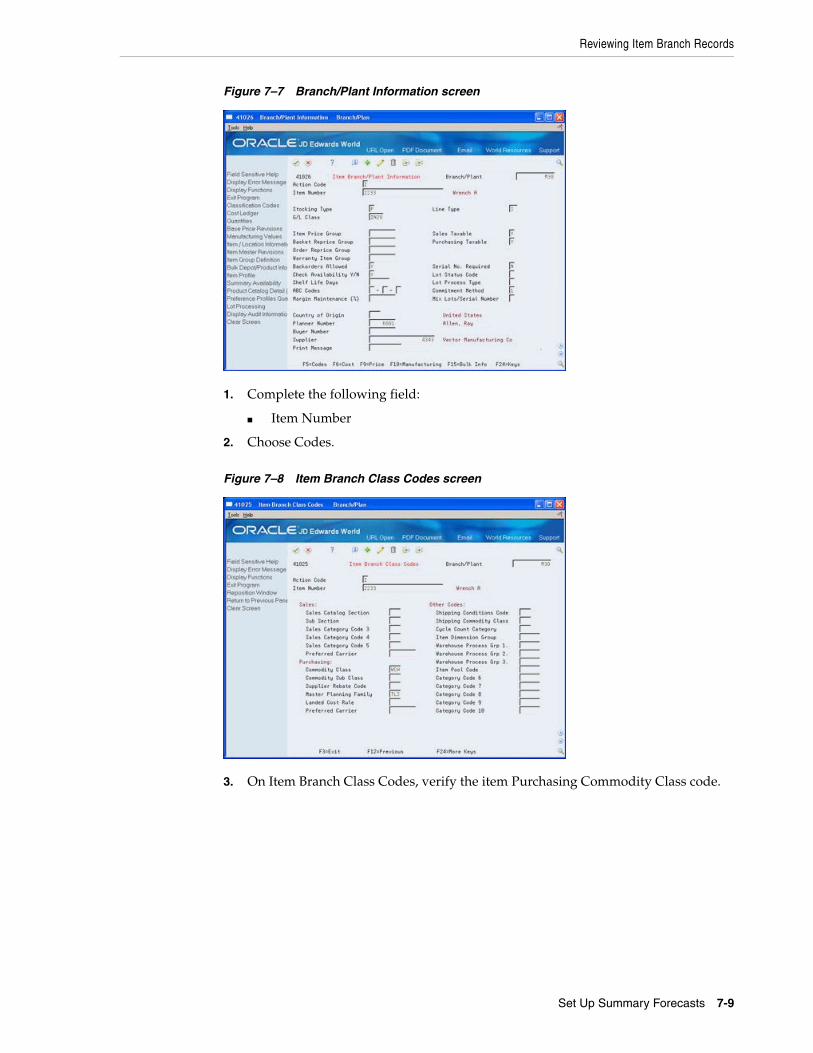
Reviewing Item Branch Records
Set Up Summary Forecasts 7-9
Figure 7–7 Branch/Plant Information screen
1. Complete the following field:
■ Item Number
2. Choose Codes.
Figure 7–8 Item Branch Class Codes screen
3. On Item Branch Class Codes, verify the item Purchasing Commodity Class code.

Reviewing Item Branch Records
7-10 JD Edwards World Forecasting Guide

8
Generate Summaries of Detail Forecasts 8-1
8Generate Summaries of Detail Forecasts
This chapter contains the topic:
■ Section 8.1, "Generating Summaries of Detail Forecasts."
8.1 Generating Summaries of Detail Forecasts
NavigationFrom Material Planning Operations (G34), choose Forecasting
From Periodic Forecasting Operations (G3421), choose Summarize Detail Forecasts
Summarize Detail Forecasts generates summary forecasts, which are stored in the Summary Forecast table (F3400), based on data from the Detail Forecast table (F3460).
This program allows you to use detail data to generate summary forecasts that provide both sales amount and item quantity data. You can summarize Detail Actual Sales data or forecasted data.
The Detail Forecast table is based on both input copied from the Sales History table (F42119) using Extract Sales Order History and input generated by the Generate Detail Forecast program.

Generating Summaries of Detail Forecasts
8-2 JD Edwards World Forecasting Guide
Figure 8–1 Detail Forecast Table
You do not need to clear the Summary Forecast table before you run this program. The program deletes any forecasts in the table for the summary code that you specify. If you enter From/Thru dates, the system only deletes those forecasts within the date range. The program adds the forecast amounts to the selected record and then to every record in the hierarchy above it.
8.1.1 Before You Begin ■ Run the Generate Detail Forecast program
8.1.2 What You Should Know About
8.1.3 Processing OptionsSee Section 18.2, "Forecast Generation (P34650)."
See Section 18.3, "Forecast Summary (P34600)."
Topic Description
Items from summary constants
Proper data selection is critical to accurate processing. You should include only items in the summary constants hierarchy.

9
Work with Summaries of Forecasts 9-1
9Work with Summaries of Forecasts
This chapter contains these topics:
■ Section 9.1, "Reviewing a Summary Forecast,"
■ Section 9.2, "Revising a Summary Forecast,"
■ Section 9.3, "Revising Summary Forecasts Using Force Changes."
After generating the forecasts, you can compare them to actual sales order histories. You can then revise both history and forecast data according to your own criteria.
When you review summaries of forecasts, you can also access a previously generated forecast. You can access a date range to display the sales order history and the forecast of item quantities or sales amounts. Then, you can compare actual sales to the forecast.
You can also specify the summary code (SUM) in the processing option to access records by planner, master family, or both.
When you revise summaries of forecasts, you revise information in a specific level of the forecast. You can also use the Force Changes program to apply changes you made to the summary up the hierarchy, down the hierarchy, or in both directions.
Before You Begin ■ Generate a summary forecast or a summary of detail forecast. See Section 13.1,
"Generating Summary Forecasts" or Section 8.1, "Generating Summaries of Detail Forecasts."
■ Enter the summary code you want to access in the appropriate processing option.
9.1 Reviewing a Summary Forecast
NavigationFrom Material Planning Operations (G34), choose Forecasting
From Periodic Forecasting Operations (G3421), choose Enter/Change Summaries
When you review summaries of forecasts, you can also access a previously generated forecast. You can access a date range to display the sales order history and the forecast of item quantities or sales amounts. Then, you can compare actual sales to the forecast.
To review a summary forecast On Enter/Change Summaries

Reviewing a Summary Forecast
9-2 JD Edwards World Forecasting Guide
Figure 9–1 Enter/Change Summaries screen
1. Complete the following fields:
■ Company
■ Location or Branch
2. Review the following fields:
■ Level
■ Forecast Quantity Original
■ Forecast Quantity Adjusted
■ Sales History Original
■ Sales History Adjusted
3. Toggle to display amount information.
4. Review the following fields:
■ Forecast Amount Original
■ Forecast Amount Adjusted
■ Sales Amount Original
■ Sales Amount Adjusted
5. Access Forecast Summary Detail.
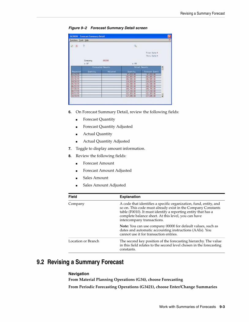
Revising a Summary Forecast
Work with Summaries of Forecasts 9-3
Figure 9–2 Forecast Summary Detail screen
6. On Forecast Summary Detail, review the following fields:
■ Forecast Quantity
■ Forecast Quantity Adjusted
■ Actual Quantity
■ Actual Quantity Adjusted
7. Toggle to display amount information.
8. Review the following fields:
■ Forecast Amount
■ Forecast Amount Adjusted
■ Sales Amount
■ Sales Amount Adjusted
9.2 Revising a Summary Forecast
NavigationFrom Material Planning Operations (G34), choose Forecasting
From Periodic Forecasting Operations (G3421), choose Enter/Change Summaries
Field Explanation
Company A code that identifies a specific organization, fund, entity, and so on. This code must already exist in the Company Constants table (F0010). It must identify a reporting entity that has a complete balance sheet. At this level, you can have intercompany transactions.
Note: You can use company 00000 for default values, such as dates and automatic accounting instructions (AAIs). You cannot use it for transaction entries.
Location or Branch The second key position of the forecasting hierarchy. The value in this field relates to the second level chosen in the forecasting constants.

Revising a Summary Forecast
9-4 JD Edwards World Forecasting Guide
After reviewing the forecasts, you can compare them to actual sales order histories. You can then revise both forecast data according to your own criteria.
You can access other revision forms, such as Force Changes, by entering options from Enter/Change Summaries. The formats vary, depending on the summary level that you view. Subsequent revision forms maintain the hierarchy level and From/Thru dates from Enter/Change Summaries.
If you run the Generate Summary Forecast program to update the Summary Forecast table, the revision forms do not display lower-level forecasts of item quantities. However, if you run Summarize Detail Forecasts to update the Summary Forecast table, these forms display the lower-level forecasts of item quantities.
To revise a summary forecast On Enter/Change Summaries
Figure 9–3 Enter/Change Summaries (Revise Summary Forecast) screen
1. Complete the following fields:
■ Company
■ Location or Branch
2. Access Forecast Summary Revisions.

Revising a Summary Forecast
Work with Summaries of Forecasts 9-5
Figure 9–4 Forecast Summary Revisions screen
3. On Forecast Summary Revisions, complete the following fields:
■ From Date
■ Thru Date
■ Change Type
■ Change Amount
■ Requested
■ Quantity Adjusted
■ Amount Forecast Adjusted
4. Complete the fields that appear based on summary constants.
5. Access the detail area.
Figure 9–5 Forecast Summary Revisions (Fields Entered) screen
6. Complete the following fields:

Revising Summary Forecasts Using Force Changes
9-6 JD Edwards World Forecasting Guide
■ Change Type
■ Change Amount
■ Pass
7. To apply the changes to higher or lower levels in the hierarchy, access Force Changes to submit adjustments to the Force Changes program.
See Section 9.3, "Revising Summary Forecasts Using Force Changes."
9.2.1 Processing OptionsSee Section 18.4, "Forecast Summary Inquiry (P34200)."
9.3 Revising Summary Forecasts Using Force Changes
NavigationFrom Material Planning Operations (G34), choose Forecasting
Field Explanation
From Date The beginning date of the range in a search. If you do not specify a beginning date, the system uses the current date.
Thru Date A numeric code that identifies either the period number or the date that you want to locate. If you leave this field blank, the system uses the ending date of the current period that is set up for the company. Valid period numbers are 1 through 14.
Change Type A field that tells the system whether the number in the New Price field is an amount or a percentage. Codes are:
A – Amount
% – Percentage
Change Amount The amount of the future change in unit price. This number can be either a dollar amount or a percentage value. If the next field (Column Title = PT) is a $ sign, the change is in dollars; if the value is a % sign, the change is to be a percentage of the current price.
Note: When entering a percentage, enter it as a whole number. For example:
Form-specific information
The change type determines whether this value is expressed as an amount or percentage.
Quantity Adjusted The quantity of units forecasted for production during a planning period.
Amount Extended Price The number of units multiplied by the unit price.
Form-specific information
The original dollar amount of the forecasted units for a planning period.
Forecast Amount The current amount of the forecasted units for a planning period.
Pass This indicates whether to bypass the force changes program. A Y indicates that the quantity and amount of a forecast should not be changed by an adjustment made to a forecast higher or lower in the hierarchy.

Revising Summary Forecasts Using Force Changes
Work with Summaries of Forecasts 9-7
From Periodic Forecasting Operations (G3421), choose Force Changes
Force Changes enables you to apply the manual changes that you made to the summary of a forecast either up the hierarchy (aggregation), down the hierarchy (disaggregation), or in both directions. The system stores these changes in the Summary Forecast table. You can access the Force Changes program in the following ways:
■ From Periodic Forecasting
■ From Forecast Summary Revisions, after you revise forecast data
The program makes changes down the hierarchy to the lowest detail level. These changes are also updated in the Detail Forecast table.
You can force changes to quantities, amounts, or both.
9.3.1 Example: Using Force Changes The Force Changes program makes manual adjustments down the hierarchy by calculating what percentage each child level's original quantity or amount is of the parent level's original quantity or amount. For example:
■ The parent's original amount is 200 and its two children in the next level have an original amount of 70 and 130, respectively. The program calculates that the first child is 35% of the parent and the second child is 65% of the parent.
■ The system maintains the parent/child ratio when the parent quantity changes. When the adjusted amount of the parent increases to 280, the adjusted amounts for the children become 70 + (35% of 80) = 98 and 130 + (65% of 80) = 182, respectively.
Figure 9–6 Force Changes
When forcing the changes up the hierarchy, the program summarizes each record again so that the summarized total of the records above it reflects the adjusted amount.

Revising Summary Forecasts Using Force Changes
9-8 JD Edwards World Forecasting Guide
Because a summarized forecast is more accurate than a detailed forecast, the forecast of total sales for the West region is more accurate than the forecast of sales of hammer 5566.
9.3.2 Before You Begin ■ Review and revise the summary forecast
■ Choose processing options to indicate:
■ The summary code for the hierarchy that you want to work with
■ A specific forecast type with which to make changes
■ The direction that you want to make changes
9.3.3 What You Should Know About
9.3.4 Processing OptionsSee Section 18.5, "Forecast Forcing (P34610)."
Topic Description
Specifying bypassed records On Enter/Change Summaries, you can set the Bypass Force flag for records in the hierarchy below an adjusted record. The system subtracts the bypassed record's amounts and quantities from the parent's amounts and quantities before calculating the percentages. The system distributes the total amounts to the other children in the hierarchy that were not bypassed. You can only bypass records when you make changes down the hierarchy.
Setting the Revised Flag processing option
When you make changes both up and down the hierarchy, the flag on the record indicating that it was changed will be reset. If you force changes in only one direction, the flag will not be reset unless the processing option is set to do so. You will lose the ability to make changes in the other direction if you do this.

Part IIIPart III Aggregate Planning Forecasts
This part contains these chapters:
■ Chapter 10, "Overview to Aggregate Planning Forecasts,"
■ Chapter 11, "Understand Summary Forecasts,"
■ Chapter 12, "Work with Summary Sales Order History,"
■ Chapter 13, "Generate Summary Forecasts,"
■ Chapter 14, "Understand Planning Bill Forecasts,"
■ Chapter 15, "Set Up a Planning Bill,"
■ Chapter 16, "Generate Planning Bill Forecasts."


10
Overview to Aggregate Planning Forecasts 10-1
10Overview to Aggregate Planning Forecasts
This chapter contains these topics:
■ Section 10.1, "Objectives,"
■ Section 10.2, "About Aggregate Planning Forecasts."
10.1 Objectives■ To define the distribution hierarchy
■ To revise address book revisions
■ To review branch or plant data
■ To review item branch locations
■ To copy summary sales order history into the Summary Forecast table
■ To review and revise summary copied sales order history
■ To generate summary forecasts
■ To explode a forecast for a pseudo parent item down to the component
10.2 About Aggregate Planning ForecastsAn aggregate production plan is usually stated by product family in terms of a monetary value of production over the given planning horizon.
Factors considered in the aggregate planning activity include:
■ Sales forecasts
■ Inventory investment
■ Capital equipment utilization
■ Work force capacity
■ Skills training requirements
■ Corporate policies concerning customer service levels, overtime, and subcontracting
Summary forecasts aggregate sales history into a monetary value of sales by product family, by region, or in other groupings used as input to the aggregate production planning activity. Planning bill forecasts convert the output of the approved aggregate plan into a time-phased master schedule for buildable end item numbers.
Complete the following tasks:

About Aggregate Planning Forecasts
10-2 JD Edwards World Forecasting Guide
■ Understand summary forecasts
■ Work with summary sales order history
■ Generate summary forecasts
■ Understand planning bill forecasts
■ Set up a planning bill
■ Generate planning bill forecasts

11
Understand Summary Forecasts 11-1
11Understand Summary Forecasts
This chapter contains the topic:
■ Section 11.1, "About Summary Forecasts."
11.1 About Summary Forecasts You use summary forecasts to project demand at a product group level. Summary forecasts are also called aggregate forecasts. You can generate a summary of a detail forecast based on detail sales histories or a summary forecast based on summary actual data.
The system updates the Sales History table (F42119) with sales data from the Sales Order table (F4211) to generate summary forecasts. You copy the sales history into the Summary Forecast table (F3400) to generate summary forecasts. The system generates summary forecasts that provide information for each level of the hierarchy that you set up with summary constants. These constants are stored in the Summary Constants table (F4091). Both summary forecasts and summaries of detail forecasts are stored in the Summary Forecast table.
11.1.1 Comparing Summaries of Detail and Summary Forecasts A summary of a detail forecast uses item-level data and predicts future sales in terms of both item quantities and sales amounts.
A summary forecast uses summary data to predict future sales.
See Also:
■ Chapter 8, "Generate Summaries of Detail Forecasts."

About Summary Forecasts
11-2 JD Edwards World Forecasting Guide

12
Work with Summary Sales Order History 12-1
12Work with Summary Sales Order History
This chapter contains these topics:
■ Section 12.1, "Copying Summary Sales Order History,"
■ Section 12.2, "Reviewing and Revising Sales Order History."
The system generates summary forecasts based on sales history data that you copy from the Sales History table (F42119) into the Summary Forecast table (F3400). When you copy the sales history, you specify a date range based on the request date of the sales order. The sales history data can be distorted, however, by unusually large or small values (spikes or outliers), data entry errors, or missing demand (sales orders that were cancelled due to lack of inventory).
You should review the data in the date range you specified to identify missing or inaccurate information. You then revise the sales order history to account for inconsistencies and distortions when you generate the forecast. If you want to account for changes in sales order activity for an especially large customer, the JD Edwards World Forecasting system allows you to work with that customer's changes separately.
12.1 Copying Summary Sales Order History
NavigationFrom Material Planning Operations (G34), choose Forecasting
From Periodic Forecasting Operations (G3421), choose Extract Sales Order History
The system generates summary forecasts based on data in the Summary Forecast table. Use Extract Sales Order History to copy the sales order history (type AA) from the Sales History table to the Summary Forecast table based upon criteria that you specify.

Copying Summary Sales Order History
12-2 JD Edwards World Forecasting Guide
Figure 12–1 Extract Sales Order History
You can also choose to enter the actual sales histories manually using the Enter/Change Summaries program. The system stores sales order histories in the Summary Forecast table with forecast type AA or a type code that you designate.
You do not need to clear the Summary Forecast table before you run this program. The system automatically deletes any records that are:

Reviewing and Revising Sales Order History
Work with Summary Sales Order History 12-3
■ For the same period as the actual sales order histories to be generated
■ For the same items
■ For the same sales order history type (AA)
■ For the same branch or plant
12.1.1 Before You Begin ■ Set up detail forecasts. See Chapter 3, "Setting Up Detail Forecasts."
■ Set up the summary forecast. See Chapter 7, "Set Up Summary Forecasts."
12.1.2 Processing OptionsSee Section 17.2, "Extract Sales Order History (P3465)."
12.2 Reviewing and Revising Sales Order History
NavigationFrom Material Planning Operations (G34), choose Forecasting
From Periodic Forecasting Operations (G3421), choose Enter/Change Summaries
After you copy the sales order history into the Summary Forecast table (F3400), you should review the data for spikes, outliers, entry errors, or missing demand that might distort the forecast. You can then revise the sales order history manually to account for these inconsistencies before you generate the forecast.
Working with summary sales order history consists of:
■ Reviewing summary sales order history
■ Revising summary sales order history
■ Reviewing forecasts by type
12.2.1 Before You Begin ■ Run the Extract Sales Order History program
To review summary sales order history On Enter/Change Summaries
Note: The Extract Sales Order History program converts sales orders into the primary unit of measure and adjusts the resulting quantities.
See Also:
■ Enter Customers in the JD Edwards World Accounts Receivable Guide.

Reviewing and Revising Sales Order History
12-4 JD Edwards World Forecasting Guide
Figure 12–2 Enter/Change Summaries screen
1. Complete the following fields:
■ From Date
■ Thru Date
■ Company
■ Forecast Type
2. To view the next level lower in the hierarchy, choose Next.
3. Complete the fields that display based on summary constants.
4. For summary information, review the following fields:
■ Level
■ Forecast Quantity Original
■ Forecast Quantity Adjusted
■ Actual Amount Original
■ Actual Amount Adjusted
To revise summary sales order history On Forecast Summary Revisions

Reviewing and Revising Sales Order History
Work with Summary Sales Order History 12-5
Figure 12–3 Forecast Summary Revisions screen.
1. To change information for the entire forecast summary, complete the following fields:
■ Change Type
■ Change Amount
2. To change information for individual lines, complete the following fields:
■ Requested Date
■ Quantity Adjusted
■ Amount Forecast Adjusted
■ Pass
3. Access the detail area.
4. Complete the following fields:
■ Change Type
■ Change Amount
To review the forecast by type On Forecast Summary Detail

Reviewing and Revising Sales Order History
12-6 JD Edwards World Forecasting Guide
Figure 12–4 Forecast Summary Detail screen
1. Review the following fields:
■ Actual Quantity
■ Actual Quantity Adjusted
2. Toggle to display amount information.
3. Review the following fields:
■ Sales Amount
■ Sales Amount Adjusted
12.2.2 Processing OptionsSee Section 18.4, "Forecast Summary Inquiry (P34200)."
Field Explanation
From Date The beginning date of the range in a search. If you do not specify a beginning date, the system uses the current date.
Thru Date A numeric code that identifies either the period number or the date that you want to locate. If you leave this field blank, the system uses the ending date of the current period that is set up for the company. Valid period numbers are 1 through 14.
Company A code that identifies a specific organization, fund, entity, and so on. This code must already exist in the Company Constants table (F0010). It must identify a reporting entity that has a complete balance sheet. At this level, you can have intercompany transactions.
Note: You can use company 00000 for default values, such as dates and automatic accounting instructions (AAIs). You cannot use it for transaction entries.
13
Generate Summary Forecasts 13-1
13Generate Summary Forecasts
This chapter contains the topic:
■ Section 13.1, "Generating Summary Forecasts."
13.1 Generating Summary Forecasts
NavigationFrom Material Planning Operations (G34), choose Forecasting
From Periodic Forecasting Operations (G3421), choose Create Summary Forecast
Generate Summary Forecast allows you to test simulated versions of future sales scenarios without having to run full detail forecasts. You can use this program to simulate and plan long-range trends because this program does not update information in the Detail Forecast table, which is used as input to DRP, MPS, and MRP generation.
You can also use this program to:
■ Specify the summary code for the hierarchy for which you want to forecast.
■ Generate summary forecasts based on sales history.
■ Select a best fit forecast.
■ Store any or all of the forecast methods in the Summary Forecast table.
■ Generate the forecast in a fiscal date pattern you select.
If you use the default type codes in the system's processing options, the actual sales history records are indicated by type AA, and the best fit model is indicated by type BF. The system saves the BF type and AA records (or corresponding type codes that you designate) in the Summary Forecast table. However, the other forecast types 01 through 12 are not automatically saved unless you set a processing option to do so.
You can also choose to include actual sales orders in your forecast by setting the appropriate processing options when you generate the forecast table. Including actual sales orders enables you to consider current sales activity in the forecasting process, which can enhance forecasting and planning accuracy.
When you run Generate Summary Forecast, the system:
■ Extracts sales order history information from the Summary Forecast table
■ Calculates the forecasts using methods that you select
■ Determines the percent of accuracy or mean absolute deviation for each selected forecast method

Generating Summary Forecasts
13-2 JD Edwards World Forecasting Guide
■ Recommends the best fit forecast method
■ Generates the summary forecast in both monetary amounts and units from the best fit forecast
13.1.1 Before You Begin ■ Run the Extract Sales Order History program
■ Make any changes to the sales order history with the Enter/Change Actuals program
■ On Generate Summary Forecast, set processing option "Dollar/Unit Forecast" to forecast summary amounts
13.1.2 Processing OptionsSee Section 19.3, "Summary Forecast Generation (P34640)."
Note: To generate summary forecasts for item quantities on all levels of the hierarchy, first generate a detail forecast. Next, run the Summarize Detail Forecasts program.

14
Understand Planning Bill Forecasts 14-1
14Understand Planning Bill Forecasts
This chapter contains these topics:
■ Section 14.1, "About Planning Bill Forecasts,"
■ Section 14.2, "Exploding the Forecast to the Item Level."
14.1 About Planning Bill ForecastsPlanning bills are groups of items in a bill of material format that reflect how an item is sold, rather than how it is built. Planning bills allow you to account for the variety of possible options and features that might be included as components in a saleable end item.
You can use a planning bill to configure a hypothetical average parent item that is not actually manufactured, but represents the components needed to satisfy demand for all the combinations of options and features that you expect to sell. For example, if your sales history shows that of all the bikes you sell, 60% are 10-speeds and 40% are 15-speeds, your planning bill includes an average parent bike that is neither a 10-speed nor a 15-speed, but a hybrid pseudo bike that is 60% 10-speed and 40% 15-speed.
Use planning bills during master scheduling and/or material planning. You can forecast with a planning bill to determine component demand within the MPS, MRP, and DRP systems.
14.1.1 Example: Pseudo Parent Item Your sales history shows that 60% of the bikes that you sell are 10-speeds and 40% are 15-speeds. For 10-speeds, 70% are blue and 30% are green. For 15-speeds, 80% are blue and 20% are green. You use these percentages to configure a pseudo parent item.
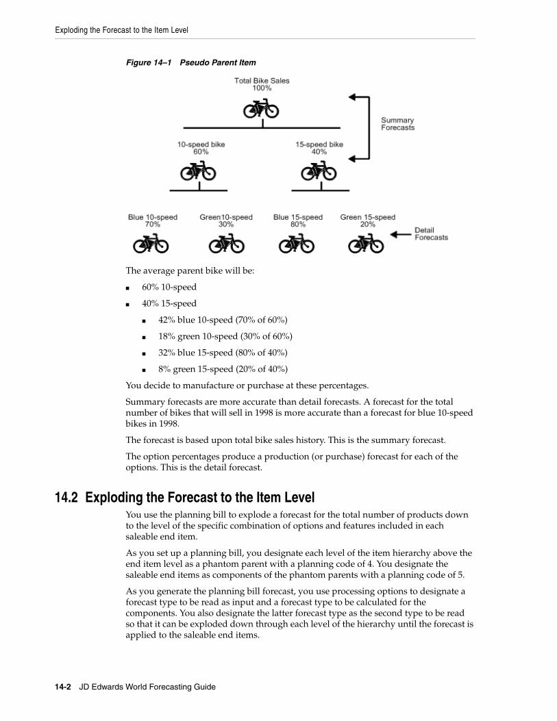
Exploding the Forecast to the Item Level
14-2 JD Edwards World Forecasting Guide
Figure 14–1 Pseudo Parent Item
The average parent bike will be:
■ 60% 10-speed
■ 40% 15-speed
■ 42% blue 10-speed (70% of 60%)
■ 18% green 10-speed (30% of 60%)
■ 32% blue 15-speed (80% of 40%)
■ 8% green 15-speed (20% of 40%)
You decide to manufacture or purchase at these percentages.
Summary forecasts are more accurate than detail forecasts. A forecast for the total number of bikes that will sell in 1998 is more accurate than a forecast for blue 10-speed bikes in 1998.
The forecast is based upon total bike sales history. This is the summary forecast.
The option percentages produce a production (or purchase) forecast for each of the options. This is the detail forecast.
14.2 Exploding the Forecast to the Item Level You use the planning bill to explode a forecast for the total number of products down to the level of the specific combination of options and features included in each saleable end item.
As you set up a planning bill, you designate each level of the item hierarchy above the end item level as a phantom parent with a planning code of 4. You designate the saleable end items as components of the phantom parents with a planning code of 5.
As you generate the planning bill forecast, you use processing options to designate a forecast type to be read as input and a forecast type to be calculated for the components. You also designate the latter forecast type as the second type to be read so that it can be exploded down through each level of the hierarchy until the forecast is applied to the saleable end items.

Exploding the Forecast to the Item Level
Understand Planning Bill Forecasts 14-3
14.2.1 Example: Exploding the Forecast You use a planning bill to configure an average parent item that represents total bike sales. This pseudo parent bike represents the top level of the item hierarchy and is configured as follows:
■ 60% 10-speed
■ 40% 15-speed
Because bikes with both the 10-speed and 15-speed options can be further divided into blue and green bikes, both the total of all 10-speed bikes and the total of all 15-speed bikes are represented by phantom parent bikes on the second level of the item hierarchy. These phantom parents are configured as follows:
■ 10-speed:
■ 70% blue
■ 30% green
■ 15-speed:
■ 80% blue
■ 20% green
The system enables you to process multiple parent items as in this example. You use planning code 4 to designate each of the phantom products on the two higher levels of the hierarchy (total bikes on the top level and total 10-speeds and total 15-speeds on the second level) as parent items. You use planning code 5 to designate the end item bikes (for example, blue 15-speeds) on the bottom level as components of the phantom parent items.
You assign user defined codes to several additional forecast types you want to include in the processing options to supplement the types that come with the system. For this forecast, you plan to use forecast types you have defined and assigned to codes 13 and 16. You designate 16 in processing options as the forecast type to be read as input for the top-level parent item and 13 as the forecast type to be created for calculating the forecast for the components.
The system reads the forecast for total bike sales determined by forecast type 16 and assign a percentage of the total forecast to each of the portions of the total on the next level of the hierarchy (total 10-speed and total 15-speed sales).
These percentages are based on "feature planned percents," the percentage of total products that include particular features that differentiate some products in the total from others. You define the feature planned percent on the Enter/Change Bill form. In this example, the feature planned percents are 60% for the 10-speed feature and 40% for the 15-speed feature.
The system then calculates a forecast based on forecast type 13 that it applies to the next level. You also designate 13 as the second forecast type to be read as input so the system will read the forecast for the second level, which it will then apply to the saleable end items (blue and green 10-speeds and blue and green 15-speeds).
The system reads forecast type 16 and calculates a type 13 forecast of 20,000 total bikes. The system then reads the forecast and explodes it down the hierarchy to the end item level as follows:
■ 60% of the 20,000 total bikes = 12,000 10-speed bikes
■ 40% of the 20,000 total bikes = 8,000 15-speed bikes

Exploding the Forecast to the Item Level
14-4 JD Edwards World Forecasting Guide
■ 70% of the 12,000 10-speeds (42% of total bike sales) = 8,400 blue 10-speed bikes
■ 30% of the 12,000 10-speeds (18% of total bike sales) = 3,600 green 10-speed bikes
■ 80% of the 8,000 15-speeds (32% of total bike sales) = 6,400 blue 15-speed bikes
■ 20% of the 8,000 15-speeds (8% of total bike sales) = 1,600 green 15-speed bikes
See Also:
■ About Multi-Level Master Scheduling in the JD Edwards World Manufacturing and Distribution Planning Guide.

15
Set Up a Planning Bill 15-1
15Set Up a Planning Bill
This chapter contains these topics:
■ Section 15.1, "Setting Up Item Master Information,"
■ Section 15.2, "Entering Planning Bills."
You must set up a planning bill before you generate a planning bill forecast. You use the Product Data Management system to set up a planning bill. The system uses the planning bill to generate a forecast for the hypothetical average parent item, which it explodes to the component level.
15.1 Setting Up Item Master Information
NavigationFrom Inventory Management (G41), choose Inventory Master/Transactions
From Inventory Master/Transactions (G4111), choose Item Master Information
Before you enter the criteria that you want to use on the planning bill, you must set up item master information on which your planning is based. The system stores this information in the Item Master table (F4101).
The Branch/Plant Master table (F4102) also stores the item information. After you add item master records for appropriate part numbers, the system retrieves item information from the Branch/Plant Master table.
To set up item master information On Item Master Information
See Also:
■ Entering Item Master Information in the JD Edwards World Inventory Management Guide.

Setting Up Item Master Information
15-2 JD Edwards World Forecasting Guide
Figure 15–1 Item Master Information screen
1. Complete the following fields:
■ Product Number
■ Description
■ Stocking Type
■ General Ledger (G/L) Class
2. Choose Branch/Plant (F13).
Figure 15–2 Item Branch Information screen
3. On Item Branch Information, complete the following field:
■ Branch/Plant
4. Choose Manufacturing (F10).

Setting Up Item Master Information
Set Up a Planning Bill 15-3
Figure 15–3 Plant Manufacturing Data screen
5. On Plant Manufacturing Data, complete the following field:
■ Planning Code
6. Exit Branch/Plant Information by pressing F3.
7. On Item Branch Information, choose Codes (F5).
Figure 15–4 Item Branch Class Codes screen
8. On Item Branch Class Codes, complete the following field:
■ Master Planning Family

Setting Up Item Master Information
15-4 JD Edwards World Forecasting Guide
15.1.1 Processing OptionsSee Section 19.4, "Item Master Revisions (P4101)."
Field Explanation
Product No The system provides three separate item numbers plus an extensive cross-reference capability to alternate item numbers. These item numbers are:
1. Item Number (short) - An 8-digit, computer-assigned item number.
2. 2nd Item Number - The 25-digit, free-form, user defined, alphanumeric item number.
3. 3rd Item Number - Another 25-digit, free-form, user defined, alphanumeric item number.
In addition to these three basic item numbers, an extensive cross-reference search capability has been provided (see XRT). Numerous cross-references to alternate part numbers can be user defined (for example, substitute item numbers, replacements, bar codes, customer numbers, or supplier numbers).
Form-specific information
The second of three identifiers that you can assign to an item. This field is alphanumeric.
If you leave the third identifier field blank, the system copies this number to that field.
Stocking Type A user defined code (41/I) that indicates how you stock an item (for example, as finished goods, or as raw materials). The following stocking types are hard-coded and you should not change them:
B – Bulk floor stock
C – Configured item
F – Feature
K – Kit parent item
N – Non-stock
Planning Code A code that indicates how Master Production Schedule (MPS), Material Requirements Planning (MRP), or Distribution Requirements Planning (DRP) processes this item. Valid codes are:
0 – Not Planned by MPS, MRP, or DRP
1 – Planned by MPS or DRP
2 – Planned by MRP
3 – Planned by MRP with additional independent forecast
4 – Planned by MPS, Parent in Planning Bill
5 – Planned by MPS, Component in Planning Bill
These codes are hard-coded.
Master Planning Family A code (table 41/P4) that represents an item property type or classification, such as commodity type, planning family, or so forth. The system uses this code to sort and process like items.
This field is one of six classification categories available primarily for purchasing purposes.

Entering Planning Bills
Set Up a Planning Bill 15-5
15.2 Entering Planning Bills
NavigationFrom Product Data Management (G30), choose Daily PDM Discrete
From Daily PDM Discrete (G3011), choose Enter/Change Bill
You enter a planning bill in the Product Data Management system to change the percentages on which the hypothetical average parent item is based. This allows you to account for any planning variations on which you might want to base forecasts.
To enter planning bills On Enter/Change Bill
Figure 15–5 Enter/Change Bill screen
1. Complete the following fields:
■ Branch/Plant
■ Parent Item
2. Access the detail area.

Entering Planning Bills
15-6 JD Edwards World Forecasting Guide
Figure 15–6 Enter/Change Bill (With Fields) screen
3. Complete the following fields:
■ Component Item
■ Quantity Per
■ Feature Plan Percent
The following field contains default information:
■ Issue Type Code
4. Exit to the Daily PDM Discrete menu by pressing F3.
5. Access Multi Level Bill Inquiry.
Figure 15–7 Multi Level Bill Inquiry screen
6. On Multi Level Bill Inquiry, complete the following fields:
■ Parent Item
■ Branch/Plant

Entering Planning Bills
Set Up a Planning Bill 15-7
7. To review exploded percentages, access the detail area.
Figure 15–8 Multi Level Bill Inquiry (Detail) screen
Field Explanation
Branch/Plant A code that represents a high-level business unit. It can be used to reference a branch or plant that might have departments or jobs, which represent lower-level business units (data item MCU), subordinate to it. For example:
■ Branch/Plant (MMCU)
■ Dept A (MCU)
■ Dept B (MCU)
■ Job 123 (MCU)
Business unit security is based on the higher-level business unit.
Form-specific information
An inquiry field for a branch or plant code to which an item is assigned. This field is required.
Quantity Per The number of units to which the system applies the transaction.
Form-specific information
A number that indicates how many components you use to manufacture the parent item. A quantity of zero is valid. The default value is 1.
Feature Planned % The percentage of demand for a specified feature based on projected sales. For example, a company might sell 35% of their computers with a standard keyboard and 65% of them with an extended keyboard, based on customer demand.
The Material Planning system uses this percentage to accurately plan for a feature's component items. Enter percents as whole numbers: 5% as 5.0. The default value is 100%.

Entering Planning Bills
15-8 JD Edwards World Forecasting Guide
15.2.1 Processing OptionsSee Section 19.5, "Bill of Material Revisions (P3002)."
I A code that defines how the system issues each component in the bill of material from stock. In shop floor control, it indicates how the system issues a part to a work order. Valid codes are:
I – Manual issue (default)
F – Floor stock (no issue)
B – Backflush (when part is reported as complete)
P – Preflush (when parts list is generated)
U – Super backflush (at pay-point operation)
S – Sub-contract item (send to supplier)
Blank – Shippable end item
You can issue a component in more than one way within a specific branch/plant by using a different code on the bill of material and work order parts list. The bill of material code overrides the branch/plant value.
Field Explanation

16
Generate Planning Bill Forecasts 16-1
16Generate Planning Bill Forecasts
This chapter contains the topic:
■ Section 16.1, "Generating Planning Bill Forecasts."
16.1 Generating Planning Bill Forecasts
NavigationFrom Material Planning Operations (G34), choose Single Site Planning
From Single Site Planning Operations (G3422), choose DRP Regeneration
After setting up a planning bill, you can generate a planning bill forecast to help you plan configurations for end products. The material planning generation program reads the detail forecast for the selected parent planning bill items and explodes it to create a forecast for the planning bill components for the same time periods.
16.1.1 Before You Begin ■ Enter a planning bill. See Section 15.2, "Entering Planning Bills."
■ Run Enter/Change Forecast manually to add the forecast for the parent item.
16.1.2 Processing OptionsSee Gross Regeneration in the JD Edwards World Manufacturing and Distribution Planning Guide.

Generating Planning Bill Forecasts
16-2 JD Edwards World Forecasting Guide

Part IVPart IV Processing Options
This part contains these chapters:
■ Chapter 17, "Detail Forecasts Processing Options,"
■ Chapter 18, "Summary Forecasts Processing Options,"
■ Chapter 19, "Aggregate Planning Forecasts Processing Options."


17
Detail Forecasts Processing Options 17-1
17Detail Forecasts Processing Options
This chapter contains these topics:
■ Section 17.1, "Supply/Demand Inclusion Rules (P34004),"
■ Section 17.2, "Extract Sales Order History (P3465),"
■ Section 17.3, "Forecast Generation (P34650),"
■ Section 17.4, "Forecast Review (P34201),"
■ Section 17.5, "Forecast Revisions (P3460)."
17.1 Supply/Demand Inclusion Rules (P34004)
17.2 Extract Sales Order History (P3465)
Processing Option Processing Options Requiring Further Description
DOCUMENT TYPES:
1. Enter the Document Types for Work Order and Rate you want to setup Inclusion Rules for. The document types can be stacked one after the other for multiple document types.
If left blank, 'WOSC' will be used.
Processing Option Processing Options Requiring Further Description
PROCESS CONTROL:
1. Enter the Forecast Type for creating actuals.
2. Enter the date range for creating actuals and summarized forecasts:
a. From Date (Required)
b. Thru Date (Optional)
3. Enter the version of Supply/Demand Inclusion Rules to be used for processing.
4. Enter a '1' to specify weekly buckets.
If left blank, monthly buckets will be used.

Forecast Generation (P34650)
17-2 JD Edwards World Forecasting Guide
17.3 Forecast Generation (P34650)
5. Enter a '1' to extract sales orders from F4211 as well as F42119.
If left blank, sales orders are extracted from only the sales order history file (F42119).
SUMMARY RECORDS:
6. Enter a '1' to create summary records for large customers (ABC Type = 'A').
7. Enter a '1' to base the large customer summary on the 'Ship To' address. If left blank, the 'Sold To' address will be used.
SUMMARY FORECASTS:
8. Enter a '1' to create summarized forecast records as well as detail forecast records or a '2' to create only the summarized forecast records.
If left blank, only the detail forecast records will be created.
9. Enter the Summary Code to be used to create summarized forecasts.
10. Enter a '1' if you want the Address Book number from the Forecast File to be used to retrieve the Address Book Category Codes.
If left blank, the Cost Center will be used to determine which Address Book number to use to retrieve the Category Codes.
FISCAL PATTERN:
11. Enter the Fiscal Date Pattern to use for creating actuals.
If left blank, the pattern specified for company '00000' will be used.
The Fiscal Patterns must include a 'Begin Date'. For best results, the pattern must extend to include the last Sales Order History date.
INTERBRANCH SALES ORDERS:
12. Enter a '1' to use sales branch instead of supply branch for interbranch sales orders.
13. Enter the interbranch order type(s).
To specify more than one order type, type them one after the other along this field. (e.g. 'SIS1S2')
Processing Option Processing Options Requiring Further Description
FORECASTING METHODS:
Enter a '1' by the method(s) desired:
Processing Option Processing Options Requiring Further Description

Forecast Generation (P34650)
Detail Forecasts Processing Options 17-3
1. Percent Over Last Year
a. Enter the percentage of change over last year. For example, use 1.10 for a 10% increase, or 0.97 for a 3% decrease.
2. Calculated Percent Over Last Year
a. Enter the number of periods to include in the percentage.
3. Last Year to This Year
4. Moving Average
a. Enter the number of periods to include in the average.
5. Linear Approximation
a. Enter the number of periods to include in the ratio.
6. Least Squares Regression
a. Enter the number of periods to include in regression.
7. Second Degree Approximation
a. Enter the number of periods to include.
8. Flexible Method (Percent over N periods prior.)
a. Enter the number of periods prior.
b. Enter the percent over the prior period.
9. Weighted Moving Average
a. Enter the number of periods
b. Weight for one period prior
c. Weight for two periods prior
d. Weight for three periods prior
e. Weight for four periods prior
f. Weight for five periods prior
g. Weight for six periods prior
h. Weight for seven periods prior
i. Weight for eight periods prior
j. Weight for nine periods prior
k. Weight for ten periods prior
l. Weight for eleven periods prior
m. Weight for twelve periods prior
Note: Weights must add up to 1. If weights are entered for periods greater than the number of periods to include, they will not be used.
If no weight is entered for a period within the number of periods to include, a zero weight will be used for that period.
10. Linear Smoothing
a. Enter the number of periods to include in smoothing average.
Processing Option Processing Options Requiring Further Description

Forecast Generation (P34650)
17-4 JD Edwards World Forecasting Guide
11. Exponential Smoothing
a. Enter the number of periods to include in smoothing average.
b. Enter the alpha factor. If left blank, alpha will be calculated.
12. Exponential Smoothing with Trend and Seasonality Factors
a. Enter the alpha factor.
If left blank, alpha will be calculated.
b. Enter the beta factor.
If left blank, beta will be calculated.
c. Enter a '1' to include seasonality in the calculation.
If left blank, seasonality will not be included.
RECORD TYPES TO USE:
13. Enter the 'Actual Type' in which the actual information is stored.
14. Enter the Forecast Type to use when creating forecasts.
SUMMARY RECORDS:
15. Enter a '1' to create summary records for large customers.
(ABC type = 'A'.)
FORECAST TYPE AND RANGE:
16. Enter a '1' to specify weekly forecasts.
If left blank, monthly forecasts will be generated.
17. Enter the date to start forecasts.
If left blank, today's date will be used.
18. Enter the number of periods to forecast.
If left blank, three periods will be used.
19. Enter the number of periods of actual data to be used to calculate the Best Fit forecast.
If left blank, three periods of data will be used.
20. Enter a '1' to calculate best fit using Mean Absolute Deviation.
If left blank, Percent of Accuracy will be used.
21. Enter a '1' to run the report in final mode.
If left blank, the report will run in proof mode.
22. Enter a '1' to allow negative values to be written.
If left blank, negative values will be written as zeroes.
FISCAL DATE PATTERN:
Processing Option Processing Options Requiring Further Description

Forecast Revisions (P3460)
Detail Forecasts Processing Options 17-5
17.4 Forecast Review (P34201)
17.5 Forecast Revisions (P3460)
23. Enter the Fiscal Date Pattern Type to use for forecast dating.
If left blank, the type specified for company '00000' will be used.
(See Company Names-Fiscal Patterns 'P00105' for more information).
BEST FIT AMOUNTS/QUANTITIES:
24. Enter a '1' to calculate Best Fit using amounts.
If left blank, quantities will be used to calculate Best Fit.
Processing Option Processing Options Requiring Further Description
DEFAULT VALUES:
1. Enter a '1' to display the Amount format first.
If left blank, the Quantity format will be displayed.
2. Forecast Type (Optional)
3. Enter the default forecast type for displaying the actual quantities and amounts.
Processing Option Processing Options Requiring Further Description
DEFAULT VALUES:
1. Forecast Type (Optional)
2. Enter a '1' to default the forecast type from the heading into the detail records on an add.
3. Enter a '1' to display the Amount format first.
If left blank, the Quantity format will be displayed.
Processing Option Processing Options Requiring Further Description

Forecast Revisions (P3460)
17-6 JD Edwards World Forecasting Guide

18
Summary Forecasts Processing Options 18-1
18Summary Forecasts Processing Options
This chapter contains these topics:
■ Section 18.1, "Summary Constants (P4091),"
■ Section 18.2, "Forecast Generation (P34650),"
■ Section 18.3, "Forecast Summary (P34600),"
■ Section 18.4, "Forecast Summary Inquiry (P34200),"
■ Section 18.5, "Forecast Forcing (P34610)."
18.1 Summary Constants (P4091)
18.2 Forecast Generation (P34650)
Processing Option Processing Options Requiring Further Description
PROCESSING CONTROL :
1. Enter a '1' next to the type of Category Code Key Positions you would like to see first.
If both categories are left blank then the Item format will display first.
Address Book . . . . . . .
Item . . . . . . . . . . .
Processing Option Processing Options Requiring Further Description
FORECASTING METHODS:
Enter a '1' by the method(s) desired:
1. Percent Over Last Year
a. Enter the percentage of change over last year. For example, use 1.10 for a 10% increase, or 0.97 for a 3% decrease.
2. Calculated Percent Over Last Year
a. Enter the number of periods to include in the percentage.
3. Last Year to This Year

Forecast Generation (P34650)
18-2 JD Edwards World Forecasting Guide
4. Moving Average
a. Enter the number of periods to include in the average.
5. Linear Approximation
a. Enter the number of periods to include in the ratio.
6. Least Squares Regression
a. Enter the number of periods to include in regression.
7. Second Degree Approximation
a. Enter the number of periods to include.
8. Flexible Method (Percent over N periods prior.)
a. Enter the number of periods prior.
b. Enter the percent over the prior period.
9. Weighted Moving Average
a. Enter the number of periods
b. Weight for one period prior
c. Weight for two periods prior
d. Weight for three periods prior
e. Weight for four periods prior
f. Weight for five periods prior
g. Weight for six periods prior
h. Weight for seven periods prior
i. Weight for eight periods prior
j. Weight for nine periods prior
k. Weight for ten periods prior
l. Weight for eleven periods prior
m. Weight for twelve periods prior
Note: Weights must add up to 1. If weights are entered for periods greater than the number of periods to include, they will not be used.
If no weight is entered for a period within the number of periods to include, a zero weight will be used for that period.
10. Linear Smoothing
a. Enter the number of periods to include in smoothing average.
11. Exponential Smoothing
a. Enter the number of periods to include in smoothing average.
b. Enter the alpha factor. If left blank, alpha will be calculated.
Processing Option Processing Options Requiring Further Description

Forecast Generation (P34650)
Summary Forecasts Processing Options 18-3
12. Exponential Smoothing with Trend and Seasonality Factors
a. Enter the alpha factor.
If left blank, alpha will be calculated.
b. Enter the beta factor.
If left blank, beta will be calculated.
c. Enter a '1' to include seasonality in the calculation.
If left blank, seasonality will not be included.
RECORD TYPES TO USE:
13. Enter the 'Actual Type' in which the actual information is stored.
14. Enter the Forecast Type to use when creating forecasts.
SUMMARY RECORDS:
15. Enter a '1' to create summary records for large customers.
(ABC type = 'A'.)
FORECAST TYPE AND RANGE:
16. Enter a '1' to specify weekly forecasts.
If left blank, monthly forecasts will be generated.
17. Enter the date to start forecasts.
If left blank, today's date will be used.
18. Enter the number of periods to forecast.
If left blank, three periods will be used.
19. Enter the number of periods of actual data to be used to calculate the Best Fit forecast.
If left blank, three periods of data will be used.
20. Enter a '1' to calculate best fit using Mean Absolute Deviation.
If left blank, Percent of Accuracy will be used.
21. Enter a '1' to run the report in final mode.
If left blank, the report will run in proof mode.
22. Enter a '1' to allow negative values to be written.
If left blank, negative values will be written as zeroes.
FISCAL DATE PATTERN:
23. Enter the Fiscal Date Pattern Type to use for forecast dating.
If left blank, the type specified for company '00000' will be used.
(See Company Names-Fiscal Patterns 'P00105' for more information).
BEST FIT AMOUNTS/QUANTITIES:
Processing Option Processing Options Requiring Further Description

Forecast Summary (P34600)
18-4 JD Edwards World Forecasting Guide
18.3 Forecast Summary (P34600)
18.4 Forecast Summary Inquiry (P34200)
18.5 Forecast Forcing (P34610)
24. Enter a '1' to calculate Best Fit using amounts.
If left blank, quantities will be used to calculate Best Fit.
Processing Option Processing Options Requiring Further Description
PROCESSING CONTROL:
1. Enter the Summary Code.
2. Enter the Forecast Type.
3. Enter the Date Range:
a. From Date
b. Thru Date
4. Enter a '1' to use the Address Book Number from the Forecast file (F3460) to retrieve Category Codes.
If left blank, the Address Book Number from the Cost Center will be used.
Processing Option Processing Options Requiring Further Description
DEFAULT INFORMATION:
1. Summary Code
2. Enter Forecast Types for the following:
a. Forecast
b. Actual
3. Enter a '1' to display the Quantity format first.
If left blank, the Amount format will be displayed.
DREAM WRITER VERSIONS:
Enter the version for each program.
If left blank, 'ZJDE0001' will be used.
4. Summary Revisions (P3400)
5. Detail Revisions (P3460)
Processing Option Processing Options Requiring Further Description
PROCESSING CONTROL:
Processing Option Processing Options Requiring Further Description
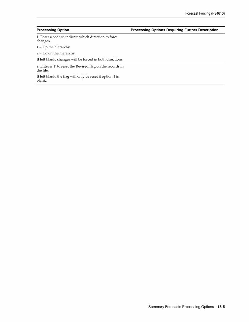
Forecast Forcing (P34610)
Summary Forecasts Processing Options 18-5
1. Enter a code to indicate which direction to force changes.
1 = Up the hierarchy
2 = Down the hierarchy
If left blank, changes will be forced in both directions.
2. Enter a '1' to reset the Revised flag on the records in the file.
If left blank, the flag will only be reset if option 1 is blank.
Processing Option Processing Options Requiring Further Description

Forecast Forcing (P34610)
18-6 JD Edwards World Forecasting Guide

19
Aggregate Planning Forecasts Processing Options 19-1
19Aggregate Planning Forecasts Processing Options
This chapter contains these topics:
■ Section 19.1, "Extract Sales Order History (P3465),"
■ Section 19.2, "Forecast Summary Inquiry (P34200),"
■ Section 19.3, "Summary Forecast Generation (P34640),"
■ Section 19.4, "Item Master Revisions (P4101),"
■ Section 19.5, "Bill of Material Revisions (P3002),"
■ Section 19.6, "Master Planning Schedule - Plant Maintenance (P3482)."
19.1 Extract Sales Order History (P3465)
Processing Option Processing Options Requiring Further Description
PROCESS CONTROL:
1. Enter the Forecast Type for creating actuals.
2. Enter the date range for creating actuals and summarized forecasts:
a. From Date (Required)
b. Thru Date (Optional)
3. Enter the version of Supply/Demand Inclusion Rules to be used for processing.
4. Enter a '1' to specify weekly buckets.
If left blank, monthly buckets will be used.
5. Enter a '1' to extract sales orders from F4211 as well as F42119.
If left blank, sales orders are extracted from only the sales order history file (F42119).
SUMMARY RECORDS:
6. Enter a '1' to create summary records for large customers (ABC Type = 'A').
7. Enter a '1' to base the large customer summary on the 'Ship To' address. If left blank, the 'Sold To' address will be used.

Forecast Summary Inquiry (P34200)
19-2 JD Edwards World Forecasting Guide
19.2 Forecast Summary Inquiry (P34200)
SUMMARY FORECASTS:
8. Enter a '1' to create summarized forecast records as well as detail forecast records or a '2' to create only the summarized forecast records.
If left blank, only the detail forecast records will be created.
9. Enter the Summary Code to be used to create summarized forecasts.
10. Enter a '1' if you want the Address Book number from the Forecast File to be used to retrieve the Address Book Category Codes.
If left blank, the Cost Center will be used to determine which Address Book number to use to retrieve the Category Codes.
FISCAL PATTERN:
11. Enter the Fiscal Date Pattern to use for creating actuals.
If left blank, the pattern specified for company '00000' will be used.
The Fiscal Patterns must include a 'Begin Date'. For best results, the pattern must extend to include the last Sales Order History date.
INTERBRANCH SALES ORDERS:
12. Enter a '1' to use sales branch instead of supply branch for interbranch sales orders.
13. Enter the interbranch order type(s).
To specify more than one order type, type them one after the other along this field. (e.g. 'SIS1S2')
Processing Option Processing Options Requiring Further Description
DEFAULT INFORMATION:
1. Summary Code
2. Enter Forecast Types for the following:
a. Forecast
b. Actual
3. Enter a '1' to display the Quantity format first.
If left blank, the Amount format will be displayed.
DREAM WRITER VERSIONS:
Enter the version for each program.
If left blank, 'ZJDE0001' will be used.
4. Summary Revisions (P3400)
5. Detail Revisions (P3460)
Processing Option Processing Options Requiring Further Description

Summary Forecast Generation (P34640)
Aggregate Planning Forecasts Processing Options 19-3
19.3 Summary Forecast Generation (P34640)
Processing Option Processing Options Requiring Further Description
FORECASTING METHODS:
Enter a '1' by the method(s) desired.
1. Percent Over Last Year
a. Enter the percentage of change over last year. For example, use 1.10 for a 10% increase, or 0.97 for a 3% decrease.
2. Calculated Percent Over Last Year a. Enter the number of periods to include in the percentage.
3. Last Year to This Year
4. Moving Average
a. Enter the number of periods to include in the average.
5. Linear Approximation a. Enter the number of periods to include in the ratio.
6. Least Squares Regression
a. Enter the number of periods to include in regression.
7. Second Degree Approximation
a. Enter the number of periods to include.
8. Flexible Method (Percent over N periods prior.)
a. Enter the number of periods prior.
b. Enter the percent over the prior period.
9. Weighted Moving Average
a. Enter the number of periods.
b. Weight for one period prior
c. Weight for two periods prior
d. Weight for three periods prior
e. Weight for four periods prior
f. Weight for five periods prior
g. Weight for six periods prior
h. Weight for seven periods prior
i. Weight for eight periods prior
j. Weight for nine periods prior
k. Weight for ten periods prior
l. Weight for eleven periods prior
m. Weight for twelve periods prior
NOTE: Weights must add up to 1.
If weights are entered for periods greater than the number of periods to include, they will not be used.
If no weight is entered for a period within the number of periods to include, a zero weight will be used for that period.

Summary Forecast Generation (P34640)
19-4 JD Edwards World Forecasting Guide
10. Linear Smoothing
a. Enter the number of periods to include in smoothing average.
11. Exponential Smoothing
a. Enter the number of periods to include in smoothing average.
b. Enter the alpha factor.
If left blank, alpha will be calculated.
12. Exponential Smoothing with Trend and Seasonality Factors
a. Enter the alpha factor.
If left blank, alpha will be calculated.
b. Enter the beta factor.
If left blank, beta will be calculated.
c. Enter a '1' to include seasonality in the calculation.
If left blank, seasonality will not be included.
RECORD TYPES TO USE:
13. Enter the Forecast Type to use when creating forecasts.
FORECAST TYPE AND RANGE:
14. Enter a '1' to specify weekly forecasts.
If left blank, monthly forecasts will be generated.
15. Enter the date to start forecasts.
If left blank, today's date will be used.
16. Enter the number of periods to forecast.
If left blank, three periods will be used.
17. Enter the number of periods of actual data to be used to calculate the Best Fit forecast.
If left blank, three periods of data will be used.
18. Enter a '1' to calculate best fit using Mean Absolute Deviation.
If left blank, Percent of Accuracy will be used.
19. Enter a '1' to run the report in Final mode.
If left blank, the report will run in Proof mode.
20. Enter a '1' to allow negative values to be written.
If left blank, negative values will be written as zeroes.
FISCAL DATE PATTERN:
21. Enter the Fiscal Date Pattern Type to use for forecast dating.
If left blank, the type specified for company '00000' will be used.
(See Company Names-Fiscal Patterns 'P00105' for more information).
BEST FIT AMOUNTS/QUANTITIES:
Processing Option Processing Options Requiring Further Description

Item Master Revisions (P4101)
Aggregate Planning Forecasts Processing Options 19-5
19.4 Item Master Revisions (P4101)
22. Enter a '1' to calculate Best Fit using amounts.
If left blank, quantities will be used to calculate Best Fit.
Processing Option Processing Options Requiring Further Description
DEFAULT VALUES :
1. Primary Unit of Measure
(Blanks=EA)
2. Weight Unit of Measure
(Blanks=LB)
PROCESS CONTROL :
3. Specify the from and thru dates to be used for effective dates in the Item Notes File :
From Date (Blank = System date)
Thru Date (Blank = 12/31 with the year = to the default value for the data dictionary item Century Change Year (#CYR))
4. Enter a '1' for each additional Item Master information screen to display when performing an add or change.
If blank, the screen will not display.
Classification Codes
Cost Revisions (Conditional)
Price Revisions (Conditional)
Units & Measures
Manufacturing Values
Bulk Product Information
UCC Codes & UOMs
Lot Processing
5. Enter a '1' to use the window version of the screens selected above.
If left blank, the full screen versions will be displayed.
6. Enter a '1' to automatically call the Item Branch Program (P41026) when adding a new item number and return to the Item Master Screen.
Enter a '2' to call the Item Branch program automatically and remain on the Item Branch Screen.
If left blank, the Item Branch Program will not be called.
GLOBAL UPDATE:
Processing Option Processing Options Requiring Further Description

Bill of Material Revisions (P3002)
19-6 JD Edwards World Forecasting Guide
19.5 Bill of Material Revisions (P3002)
7. Enter a '1' to transfer changes made to the 2nd (LITM) and the 3rd (AITM) item numbers to the Item Branch (F4102) item records.
(F19 from Item Master Revisions allows you to update other files).
or
Enter a '2' to transfer changes to records in the selected files (see User Defined Codes 40/IC).
Press F1 to display the selected files.
DREAM WRITER VERSIONS:
Enter the version to be used for each program.
If left blank, ZJDE0001 is used.
8. Item Availability (P41202)
9. Item Branch (P41026)
10. Product Catalog Detail (P41903)
DRAWING INFORMATION:
11. Enter a '1' to protect item drawing information from update.
Processing Option Processing Options Requiring Further Description
INVENTORY VALIDATION:
1. Enter a '1' to validate for an existing Branch/Item record.
DREAM WRITER VERSIONS:
Enter the version for each program.
If left blank, 'ZJDE0001' will be used.
Note: Options 2 and 3 are used ONLY to set Printer Overrides.
2. Single-Level BOM Print (P30410)
3. Multi-Level BOM Print (P30415)
4. ECO Workbench (P30225)
5. Component Maintenance (P3015)
DREAM WRITER VERSION FROM WINDOW:
6. Enter the version of ECO Revisions (P48020) to call from the Revisions Window (P30BREV).
If left blank, version 'ZJDE0001' will be used.
COMPONENT BRANCH:
7. Enter a '1' to change the Component Branch (Additions Only) to that which is displayed at the top of the screen.
FIELD DISPLAY:
Processing Option Processing Options Requiring Further Description

Master Planning Schedule - Plant Maintenance (P3482)
Aggregate Planning Forecasts Processing Options 19-7
19.6 Master Planning Schedule - Plant Maintenance (P3482)
8. Enter a '1' by the following fields to activate them:
Bill Type
Batch Quantity
DEFAULT VALUES:
9. Bill Type (Optional)
DATE EFFECTIVITY:
10. Enter a date to default into the As of Date or '*' to display all dates.
If left blank, the system date will be used.
COMPONENT SEQUENCING:
11. Enter the sequence to be displayed:
1 - Component Line Number
2 - Operation Sequence Number
Note: If left blank, components will be sequenced by Component Line Number.
REVISION LEVEL CONTROL:
12. Enter a '1' to protect Component Revision Level from update.
Processing Option Processing Options Requiring Further Description
BUCKET INFORMATION:
1. Enter the Start Date.
If left blank, the system date will be used.
2. Enter the number of past due periods (0-2).
If left blank, there will be no past due periods.
Set to 2 if using Planning Fence Rule H.
3. Enter the planning horizon periods (maximum of 52 periods):
Days (e.g. 5 )
Weeks (e.g. 25)
Months (e.g. 6 )
Maximum of 52 including Past Due buckets
PROCESSING CONTROL:
4. Enter the Generation Mode:
1 = Net Change
2 = Gross Regeneration
5. Enter the Generation Type:
1 = Single Level MPS/DRP
2 = Planning Bill
3 = MRP
5 = MRP with Frozen MPS
PHANTOM ITEMS:
Processing Option Processing Options Requiring Further Description

Master Planning Schedule - Plant Maintenance (P3482)
19-8 JD Edwards World Forecasting Guide
6. Enter a '1' to generate messages and time series records for phantoms.
ON HAND ADJUSTMENTS:
7. Enter a '1' to decrease beginning available by safety stock quantity.
8. Enter the lot hold codes (up to 5) to be considered on hand, or enter an '*' to consider all held lots as on hand.
If left blank, held lots will not be considered on hand.
9. Enter a '1' by the following Receipt Routing quantities to be considered on hand.
Quantity in Transit
Quantity in Inspection
User Defined Quantity 1
User Defined Quantity 2
Note: Any quantity not included will be placed in the On Receipt bucket.
DAMPER DAYS:
10. Enter the Defer Damper days, (no defer message if less than 'X' number of days).
11. Enter the Expedite Damper days, (no expedite message if less than 'X' number of days).
SAFETY LEADTIME:
12. Enter the purchased item lead time days.
13. Enter the manufactured item lead time days.
FORECASTING INFORMATION:
14. Enter up to five forecast types:
Forecast Type 1
Forecast Type 2
Forecast Type 3
Forecast Type 4
Forecast Type 5
15. Enter the Forecast Type for MPS to create when using Planning Bills.
RATE BASED SCHEDULING INFORMATION:
16. Enter the Schedule Type for rate based items.
If left blank, 'SC' will be used.
17. Enter a '1' to extend rate based adjustments to lower level items.
18. Enter status code used to denote closed rates.
If left blank, 99 will be used.
19. Enter a '1' to include Past Due Rates as a supply.
PURCHASE ORDER INFORMATION:
Processing Option Processing Options Requiring Further Description

Master Planning Schedule - Plant Maintenance (P3482)
Aggregate Planning Forecasts Processing Options 19-9
20. Enter the Document Type for purchase orders.
If left blank, 'OP' will be used.
WORK ORDER INFORMATION:
21. Enter the Document Type for work orders.
If left blank, 'WO' will be used.
22. Enter the Work Order Status at which messages will no longer be exploded to lower level items.
If left blank, all messages will be exploded to lower level items.
INCLUSION RULES:
23. Enter the Version of Supply/Demand Inclusion Rules to be used.
PERFORMANCE ISSUES:
24. Enter a '1' to initialize the MPS/MRP Print Code. This code is used for selecting records during the MPS/MRP print.
(See glossary for MRPD.)
Note: If left blank, the run time of the generation will be reduced.
25. Enter the User Defined Code Type that contains the list of quantity types to be calculated & written to the Time Series file (F3413). User Defined Code 34/QT contains a master list of quantity types that can be written and will be used as the default.
26. Enter a '1' to completely clear the material planning files (messages, pegging, and time series) prior to the generation or a '2' to retain manual remarks (type M messages) while clearing the files.
Default of blank will not clear files.
Note: If a '1' or '2' is entered, files will be cleared without respect to data selection.
Clearing the files will improve performance and clean up any bad data in the files.
PROCESS PLANNING:
27. Enter a '1' to generate planning in Process Mode.
Note: If left blank, the run time of the generation will be reduced.
Processing Option Processing Options Requiring Further Description

Master Planning Schedule - Plant Maintenance (P3482)
19-10 JD Edwards World Forecasting Guide
LOT EXPIRATION:
28A. Enter a '1' to consider lot expiration dates in calculations.
28B. Enter optional date to be used for expiration calculations when processing option 28A = '1'.
If left blank, Lot expiration date will be used.
1 = Sell By Date
2 = Best Before Date
3 = User Defined Date 1
4 = User Defined Date 2
5 = User Defined Date 3
6 = User Defined Date 4
7 = User Defined Date 5
8 = Commitment Date Method from Item/Branch Master.
FORECAST CONSUMPTION PROCESSING:
29. Enter a '1' to use Forecast Consumption logic.
ROUNDING:
30. Enter a '1' to round existing Work/ Purchasing orders suggested quantity to the nearest order transaction unit of measure quantity.
Note: If left blank, no rounding will occur.
Processing Option Processing Options Requiring Further Description

A
Forecast Calculation Examples A-1
AForecast Calculation Examples
This appendix contains these topics:
■ Section A.1, "Forecast Calculation Methods,"
■ Section A.2, "Forecast Performance Evaluation Criteria,"
■ Section A.3, "Method 1 - Specified Percent Over Last Year,"
■ Section A.4, "Method 2 - Calculated Percent Over Last Year,"
■ Section A.5, "Method 3 - Last year to This Year,"
■ Section A.6, "Method 4 - Moving Average,"Section A.7, "Method 5 - Linear Approximation,"
■ Section A.7, "Method 5 - Linear Approximation,"
■ Section A.8, "Method 6 - Least Square Regression,"
■ Section A.9, "Method 7 - Second Degree Approximation,"
■ Section A.10, "Method 8 - Flexible Method,"
■ Section A.11, "Method 9 - Weighted Moving Average,"
■ Section A.12, "Method 10 - Linear Smoothing,"
■ Section A.13, "Method 11 - Exponential Smoothing,"
■ Section A.14, "Method 12 - Exponential Smoothing with Trend and Seasonality,"
■ Section A.15, "Evaluating the Forecasts,"
■ Section A.16, "Mean Absolute Deviation (MAD)."
A.1 Forecast Calculation MethodsTwelve methods of calculating forecasts are available. Most of these methods provide for limited user control. For example, the weight placed on recent historical data or the date range of historical data used in the calculations might be specified. The following examples show the calculation procedure for each of the available forecasting methods, given an identical set of historical data.
The following examples use the same 2004 and 2005 sales data to produce a 2006 sales forecast. In addition to the forecast calculation, each example includes a simulated 2005 forecast for a three month holdout period (processing option 19 = '3') which is then used for percent of accuracy and mean absolute deviation calculations (actual sales compared to simulated forecast).

Forecast Performance Evaluation Criteria
A-2 JD Edwards World Forecasting Guide
A.2 Forecast Performance Evaluation CriteriaDepending on your selection of processing options and on the trends and patterns existing in the sales data, some forecasting methods will perform better than others for a given historical data set. A forecasting method that is appropriate for one product may not be appropriate for another product. It is also unlikely that a forecasting method that provides good results at one stage of a product's life cycle will remain appropriate throughout the entire life cycle.
You can choose between two methods to evaluate the current performance of the forecasting methods. These are Mean Absolute Deviation (MAD) and Percent of Accuracy (POA). Both of these performance evaluation methods require historical sales data for a user specified period of time. This period of time is called a holdout period or periods best fit (PBF). The data in this period is used as the basis for recommending which of the forecasting methods to use in making the next forecast projection. This recommendation is specific to each product, and may change from one forecast generation to the next. The two forecast performance evaluation methods are demonstrated in the pages following the examples of the twelve forecasting methods.
A.3 Method 1 - Specified Percent Over Last YearThis method multiplies sales data from the previous year by a user specified factor; for example, 1.10 for a 10% increase, or 0.97 for a 3% decrease.
Required sales history: One year for calculating the forecast plus the user specified number of time periods for evaluating forecast performance (processing option 19).
A.3.1 Forecast CalculationUser specified factor (processing option 1a) = 1.15 in this example.
A.3.2 Simulated Forecast CalculationOctober, 2004 sales = 123 * 1.15 = 141.45
November, 2004 sales = 139 * 1.15 = 159.85
Month 2004 Sales 2005 Sales 2006 ForecastSimulated 2005 Forecast
January 125 128 147
February 132 117 135
March 115 115 132
April 137 125 144
May 122 122 140
June 130 137 158
July 141 129 148
August 128 140 161
September 118 131 151
October 123 114 131 141.45
November 139 119 137 159.85
December 133 137 158 152.95

Method 2 - Calculated Percent Over Last Year
Forecast Calculation Examples A-3
December, 2004 sales = 133 * 1.15 = 152.95
A.3.3 Percent of Accuracy CalculationPOA = (141.45 + 159.85 + 152.95) / (114 + 119 + 137) * 100 = 454.25 / 370 = 122.770
A.3.4 Mean Absolute Deviation CalculationMAD = (|141.45 - 114| + |159.85 - 119| + |152.95 - 137|) / 3 = (27.45 + 40.85 + 15.95) / 3 = 84.25/3 = 28.08
A.4 Method 2 - Calculated Percent Over Last YearThis method multiplies sales data from the previous year by a factor calculated by the system.
Required sales history: One year for calculating the forecast plus the user specified number of time periods for evaluating forecast performance (processing option 19).
A.4.1 Forecast CalculationRange of sales history to use in calculating growth factor (processing option 2a) = 3 in this example.
Sum the final three months of 2005: 114 + 119 + 137 = 370
Sum the same three months for the previous year: 123 + 139 + 133 = 395
The calculated factor = 370/395 = 0.9367
Calculate the forecasts:
January, 2005 sales = 128 * 0.9367 = 119.8036 or about 120
February, 2005 sales = 117 * 0.9367 = 109.5939 or about 110
March, 2005 sales = 115 * 0.9367 = 107.7205 or about 108
Month 2004 Sales 2005 Sales 2006 ForecastSimulated 2005 Forecast
January 125 128 120
February 132 117 110
March 115 115 108
April 137 125 117
May 122 122 114
June 130 137 128
July 141 129 121
August 128 140 131
September 118 131 123
October 123 114 107 127.13178
November 139 119 111 143.66925
December 133 137 128 137.4677

Method 3 - Last year to This Year
A-4 JD Edwards World Forecasting Guide
A.4.2 Simulated Forecast CalculationSum the three months of 2005 prior to holdout period (July, Aug, Sept):
129 + 140 + 131 = 400
Sum the same three months for the previous year:
141 + 128 + 118 = 387
The calculated factor = 400/387 = 1.033591731
Calculate simulated forecast:
October, 2004 sales = 123 * 1.033591731 = 127.13178
November, 2004 sales = 139 * 1.033591731 = 143.66925
December, 2004 sales = 133 * 1.033591731 = 137.4677
A.4.3 Percent of Accuracy CalculationPOA = (127.13178 + 143.66925 + 137.4677) / (114 + 119 + 137) * 100 = 408.26873 / 370 * 100 = 110.3429
A.4.4 Mean Absolute Deviation CalculationMAD = (|127.13178 - 114| + |143.66925 - 119| + |137.4677- 137|) / 3 = (13.13178+ 24.66925 + 0.4677)/3 = 12.75624
A.5 Method 3 - Last year to This YearThis method copies sales data from the previous year to the next year.
Required sales history: One year for calculating the forecast plus the number of time periods specified for evaluating forecast performance (processing option 19).
A.5.1 Forecast CalculationJanuary 2005 sales = January 2006 forecast = 128
Month 2004 Sales 2005 Sales 2006 ForecastSimulated 2005 Forecast
January 125 128 128
February 132 117 117
March 115 115 115
April 137 125 125
May 122 122 122
June 130 137 137
July 141 129 129
August 128 140 140
September 118 131 131
October 123 114 114 123
November 139 119 119 139
December 133 137 137 133

Method 4 - Moving Average
Forecast Calculation Examples A-5
February 2005 sales = February 2006 forecast = 117
March 2005 sales = March 2006 forecast = 115
A.5.2 Simulated Forecast CalculationOctober 2004 sales = 123
November 2004 sales = 139
December 2004 sales = 133
A.5.3 Percent of Accuracy CalculationPOA = (123 + 139 + 133) / (114 + 119 + 137) * 100 = 395/370 * 100 = 106.7567
A.5.4 Mean Absolute Deviation CalculationMAD = (|123-114| + |139 - 119| + |133 - 137|) / 3 = (9 + 20 + 4)/3 = 11
A.6 Method 4 - Moving AverageThis method averages a user specified number of months (processing option 4a) to project the next months demand.
Required sales history: Twice the number of periods to be included in the average (processing option 4a), plus number of time periods for evaluating forecast performance (processing option 19).
A.6.1 Forecast CalculationNumber of periods to be included in the average (processing option 4a) = 3 in this example
For each month of the forecast, average the previous three month's data.
January forecast: 114 + 119 + 137 = 370, 370 / 3 = 123.333 or 123
Month 2004 Sales 2005 Sales 2006 ForecastSimulated 2005 Forecast
January 125 128 123
February 132 117 126
March 115 115 129
April 137 125 126
May 122 122 127
June 130 137 127
July 141 129 127
August 128 140 127
September 118 131 127
October 123 114 127 133.3333
November 139 119 127 128.3333
December 133 137 127 121.3333

Method 5 - Linear Approximation
A-6 JD Edwards World Forecasting Guide
February forecast: 119 + 137 + 123 = 379, 379 / 3 = 126.333 or 126
March forecast: 137 + 123 + 126 = 379, 386 / 3 = 128.667 or 129
A.6.2 Simulated Forecast CalculationOctober 2005 sales = (129 + 140 + 131)/3 = 133.3333
November 2005 sales = (140 + 131 + 114)/3 = 128.3333
December 2005 sales = (131 + 114 + 119)/3 = 121.3333
A.6.3 Percent of Accuracy CalculationPOA = (133.3333 + 128.3333 + 121.3333) / (114 + 119 + 137) * 100 = 103.513
A.6.4 Mean Absolute Deviation CalculationMAD = (|133.3333 - 114| + |128.3333 - 119| + |121.3333 - 137|) / 3 = 14.7777
A.7 Method 5 - Linear ApproximationLinear Approximation calculates a trend based upon two sales history data points.
Those two points define a straight trend line that is projected into the future. Use this method with caution, as long range forecasts are leveraged by small changes in just two data points.
Required sales history: The number of periods to include in regression (processing option 5a), plus 1 plus the number of time periods for evaluating forecast performance (processing option 19).
A.7.1 Forecast CalculationNumber of periods to include in regression (processing option 5a) = 3 in this example
For each month of the forecast, add the increase or decrease during the specified periods prior to holdout period the previous period.
Month 2004 Sales 2005 Sales 2006 SalesSimulated 2005 Forecast
January 125 128 149
February 132 117 160
March 115 115 172
April 137 125 183
May 122 122 195
June 130 137 206
July 141 129 218
August 128 140 229
September 118 131 241
October 123 114 252 132
November 139 119 264 101
December 133 137 275 113

Method 6 - Least Square Regression
Forecast Calculation Examples A-7
January forecast: (137 - 114)/2 + 137 = 148.5 or 149
February forecast: (137 - 114)/2 * 2 + 137 = 160
March forecast: (137 - 114)/2 * 3 + 137 = 171.5 or 172
A.7.2 Simulated Forecast CalculationOctober 2004 sales = (131 - 129) / 2 + 131 = 132
November 2004 sales = (114 - 140) / 2 + 114 = 101
December 2004 sales = (119 - 131) /2 + 119 = 113
A.7.3 Percent of Accuracy CalculationPOA = (132 + 101 + 113) / (114 + 119 + 137) * 100 = 93.5135
A.7.4 Mean Absolute Deviation CalculationMAD = (|132 - 114| + |101 - 119| + |113 - 137|) / 3 = 20
A.8 Method 6 - Least Square RegressionLinear Regression or Least Squares Regression (LSR) is the most popular method for identifying a linear trend in historical sales data. The method calculates the values for "a" and "b" to be used in the formula: Y = a + bX. The equation describes a straight line where Y represents sales, and X represents time. Linear regression is slow to recognize turning points and step function shifts in demand. Linear regression fits a straight line to the data, even when the data is seasonal or would better be described by a curve. When the sales history data follows a curve or has a strong seasonal pattern, forecast bias and systematic errors occur.
Forecast specifications: n = identifies the periods of sales history that will be used in calculating the values for a and b. For example, specify n = 3 to use the history from October through December, 2005 as the basis for the calculations. When data is available a larger n (such as n = 24) would ordinarily be used. LSR will define a line for as few as two data points. For this example, a small value for n (n = 3) was chosen to reduce the manual calculations required to verify the results.
Required sales history: The number of periods to include in regression (processing option 6a) plus the number of time periods for evaluating forecast performance (processing option 19).
Month 2004 Sales 2005 Sales 2006 ForecastSimulated 2005 Forecast
January 125 128 146
February 132 117 158
March 115 115 169
April 137 125 181
May 122 122 192
June 130 137 204
July 141 129 215
August 128 140 227

Method 6 - Least Square Regression
A-8 JD Edwards World Forecasting Guide
A.8.1 Forecast CalculationNumber of periods to include in regression (processing option 6a) = 3 in this example
For each month of the forecast, add the increase or decrease during the specified periods prior to holdout period the previous period.
January forecast:
Average of the previous three months = (114 + 119 + 137)/3 = 123.3333
Summary of the previous three months with weight considered
= (114 * 1) + (119 * 2) + (137 * 3) = 763
Difference between the values
= 763 - 123.3333 * (1 + 2 + 3) = 23
Ratio = (1^2 + 2^2 + 3^2) - {(1 + 2 + 3)/3}^2 * 3 = 14 - 12 = 2
Value1 = Difference/Ratio = 23/2 = 11.5
Value2 = Average - value1 * ratio = 123.3333 - 11.5 * 2 = 100.3333
Forecast = (1 + n) * value1 + value2 = 4 * 11.5 + 100.3333 = 146.333 or 146
February forecast:
Forecast = 5 * 11.5 + 100.3333 = 157.8333 or 158
March forecast:
Forecast = 6 * 11.5 + 100.3333 = 169.3333 or 169
A.8.2 Simulated Forecast CalculationOctober 2004 sales:
Average of the previous three months
= (129 + 140 + 131)/3 = 133.3333
Summary of the previous three months with weight considered
= (129 * 1) + (140 * 2) + (131 * 3) = 802
Difference between the values
= 802 - 133.3333 * (1 + 2 + 3) = 2
Ratio = (1^2 + 2^2 + 3^2) - {(1 + 2 + 3)/3}^2 * 3 = 14 - 12 = 2
Value1 = Difference/Ratio = 2/2 = 1
Value2 = Average - value1 * ratio = 133.3333 - 1 * 2 = 131.3333
Forecast = (1 + n) * value1 + value2 = 4 * 1 + 131.3333 = 135.3333
September 118 131 238
October 123 114 250 135.333
November 139 119 261 102.333
December 133 137 273 109.333
Month 2004 Sales 2005 Sales 2006 ForecastSimulated 2005 Forecast

Method 7 - Second Degree Approximation
Forecast Calculation Examples A-9
November 2004 sales
Average of the previous three months
= (140 + 131 + 114)/3 = 128.3333
Summary of the previous three months with weight considered
= (140 * 1) + (131 * 2) + (114 * 3) = 744
Difference between the values = 744 - 128.3333 * (1 + 2 + 3) = -25.9999
Value1 = Difference/Ratio = -25.9999/2 = -12.9999
Value2 = Average - value1 * ratio = 128.3333 - (-12.9999) * 2 = 154.3333
Forecast = 4 * -12.9999 + 154.3333 = 102.3333
December 2004 sales
Average of the previous three months
= (131 + 114 + 119)/3 = 121.3333
Summary of the previous three months with weight considered
= (131 * 1) + (114 * 2) + (119 * 3) = 716
Difference between the values
= 716 - 121.3333 * (1 + 2 + 3) = -11.9999
Value1 = Difference/Ratio = -11.9999/2 = -5.9999
Value2 = Average - value1 * ratio = 121.3333 - (-5.9999) * 2 = 133.3333
Forecast = 4 * (-5.9999) + 133.3333 = 109.3333
A.8.3 Percent of Accuracy CalculationPOA = (135.33 + 102.33 + 109.33) / (114 + 119 + 137) * 100 = 93.78
A.8.4 Mean Absolute Deviation CalculationMAD = (|135.33 - 114| + |102.33 - 119| + |109.33 - 137|) / 3 = 21.88
A.9 Method 7 - Second Degree ApproximationLinear Regression determines values for a and b in the forecast formula Y = a + bX with the objective of fitting a straight line to the sales history data. Second Degree Approximation is similar. However, this method determines values for a, b, and c in the forecast formula Y = a + bX + cX2 with the objective of fitting a curve to the sales history data. This method may be useful when a product is in the transition between stages of a life cycle. For example, when a new product moves from introduction to growth stages, the sales trend may accelerate. Because of the second order term, the forecast can quickly approach infinity or drop to zero (depending on whether coefficient c is positive or negative). Therefore, this method is useful only in the short term.
Forecast specifications: The formulae finds a, b, and c to fit a curve to exactly three points. You specify n in the processing option 7a, the number of time periods of data to accumulate into each of the three points. In this example n = 3. Therefore, actual sales data for April through June are combined into the first point, Q1. July through September are added together to create Q2, and October through December sum to Q3. The curve will be fitted to the three values Q1, Q2, and Q3.

Method 7 - Second Degree Approximation
A-10 JD Edwards World Forecasting Guide
Required sales history: 3 * n periods for calculating the forecast plus the number of time periods required for evaluating the forecast performance (PBF).
A.9.1 Forecast CalculationNumber of periods to include (processing option 7a) = 3 in this example
Use the previous (3 * n) months in three-month blocks:
Q1(Apr - Jun) = 125 + 122 + 137 = 384
Q2(Jul - Sep) = 129 + 140 + 131 = 400
Q3(Oct - Dec) = 114 + 119 + 137 = 370
The next step involves calculating the three coefficients a, b, and c to be used in the forecasting formula Y = a + bX + cX^2
(1) Q1 = a + bX + cX^2 (where X = 1) = a + b + c
(2) Q2 = a + bX + cX^2 (where X = 2) = a + 2b + 4c
(3) Q3 = a + bX + cX^2 (where X = 3) = a + 3b + 9c
Solve the three equations simultaneously to find b, a, and c:
Subtract equation (1) from equation (2) and solve for b
(2) - (1) = Q2 - Q1 = b + 3c
b = (Q2 - Q1) - 3c
Substitute this equation for b into equation (3)
(3) Q3 = a + 3[(Q2 - Q1) - 3c] + c
a = Q3 - 3(Q2 - Q1)
Finally, substitute these equations for a and b into equation (1)
[Q3 - 3(Q2 - Q1)] + [(q2 - Q1) - 3c] + c = Q1
c = [(Q3 - Q2) + (Q1 - Q2)]/2
The Second Degree Approximation method calculates a, b, and c as follows:
Month 2004 Sales 2005 Sales 2006 ForecastSimulated 2005 Forecast
January 125 128 98
February 132 117 98
March 115 115 98
April 137 125 57
May 122 122 57
June 130 137 57
July 141 129 1
August 128 140 1
September 118 131 1
October 123 114 136
November 139 119 136
December 133 137 136

Method 8 - Flexible Method
Forecast Calculation Examples A-11
a = Q3 - 3(Q2 - Q1) = 370 - 3(400 - 384) = 322
c = [(Q3 - Q2) + (Q1 - Q2)]/2 = [(370 - 400) + (384 - 400)]/2 = -23
b = (Q2 - Q1) - 3c = (400 - 384) - (3 * -23) = 85
Y = a + bX + cX^2 = 322 + 85*X + (-23)X^2
January thru March forecast (X=4):
(322 + 340 - 368)/3 = 294/3 = 98 per period
April thru June forecast (X=5):
(322 + 425 - 575)/3 = 57.333 or 57 per period
July thru September forecast (X=6):
(322 + 510 - 828)/3 = 1.33 or 1 per period
October thru December (X=7)
(322 + 595 - 1127/3 = -70
A.9.2 Simulated Forecast CalculationOctober, November and December, 2004 sales:
Q1(Jan - Mar) = 360
Q2(Apr - Jun) = 384
Q3(Jul - Sep) = 400
a = 400 - 3(384 - 360) = 328
c = [(400 - 384) + (360 - 384)]/2 = -4
b = (384 - 360) - 3 * (-4) = 36
[328 + 36 * 4 + (-4) * 16]/3 = 136
A.9.3 Percent of Accuracy CalculationPOA = (136 + 136 + 136) / (114 + 119 + 137) * 100 = 110.27
A.9.4 Mean Absolute Deviation CalculationMAD = (|136 - 114| + |136 - 119| + |136 - 137|) / 3 = 13.33
A.10 Method 8 - Flexible MethodThe Flexible Method (Percent Over n Months Prior) is similar to Method 1, Percent Over Last Year. Both methods multiply sales data from a previous time period by a user specified factor, then project that result into the future. In the Percent Over Last Year method, the projection is based on data from the same time period in the previous year. The Flexible Method adds the capability to specify a time period other than the same period last year to use as the basis for the calculations.
Forecast specifications:
■ Multiplication factor. For example, specify 1.15 in the processing option 8b to increase the previous sales history data by 15%.
■ Base period. For example, n = 3 will cause the first forecast to be based upon sales data in October, 2005.

Method 9 - Weighted Moving Average
A-12 JD Edwards World Forecasting Guide
Minimum sales history: The user specified number of periods back to the base period, plus the number of time periods required for evaluating the forecast performance (PBF).
A.10.1 Forecast CalculationNumber of periods prior (processing option 8a) = 3, and the percent over the previous period (processing option 8b) is 1.15 in this example
For each month of the forecast, multiple the sales history n periods prior by the specified percent
January forecast: (114 * 1.15) = 131.1 or 131
February forecast: (119 * 1.15) = 136.85 or 137
March forecast: (137 * 1.15) = 157.55 or 158
A.10.2 Simulated Forecast CalculationOctober 2004 sales = 129 * 1.15 = 148.35
November 2004 sales = 140 * 1.15 = 161
December 2004 sales = 131 * 1.15 = 150.65
A.10.3 Percent of Accuracy CalculationPOA = (148 + 161 + 151) / (114 + 119 + 137) * 100 = 124.32
A.10.4 Mean Absolute Deviation CalculationMAD = (|148 - 114| + |161 - 119| + |151 - 137|) / 3 = 30
A.11 Method 9 - Weighted Moving AverageThe Weighted Moving Average (WMA) method is similar to Method 4, Moving Average (MA). However, with the Weighted Moving Average you can assign unequal
Month 2004 Sales 2005 Sales 2006 SalesSimulated 2005 Forecast
January 125 128 131
February 132 117 137
March 115 115 158
April 137 125 151
May 122 122 157
June 130 137 181
July 141 129 173
August 128 140 181
September 118 131 208
October 123 114 199 148.35
November 139 119 208 161
December 133 137 240 150.65
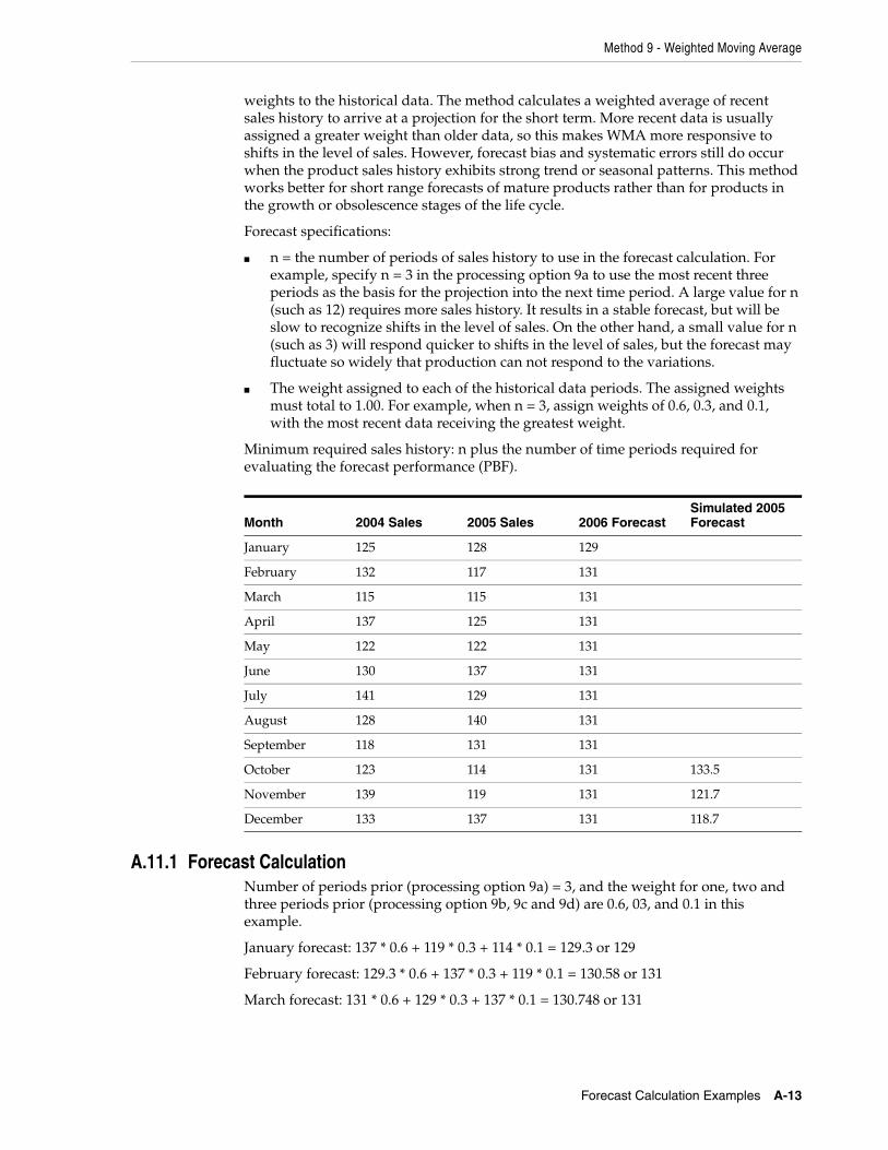
Method 9 - Weighted Moving Average
Forecast Calculation Examples A-13
weights to the historical data. The method calculates a weighted average of recent sales history to arrive at a projection for the short term. More recent data is usually assigned a greater weight than older data, so this makes WMA more responsive to shifts in the level of sales. However, forecast bias and systematic errors still do occur when the product sales history exhibits strong trend or seasonal patterns. This method works better for short range forecasts of mature products rather than for products in the growth or obsolescence stages of the life cycle.
Forecast specifications:
■ n = the number of periods of sales history to use in the forecast calculation. For example, specify n = 3 in the processing option 9a to use the most recent three periods as the basis for the projection into the next time period. A large value for n (such as 12) requires more sales history. It results in a stable forecast, but will be slow to recognize shifts in the level of sales. On the other hand, a small value for n (such as 3) will respond quicker to shifts in the level of sales, but the forecast may fluctuate so widely that production can not respond to the variations.
■ The weight assigned to each of the historical data periods. The assigned weights must total to 1.00. For example, when n = 3, assign weights of 0.6, 0.3, and 0.1, with the most recent data receiving the greatest weight.
Minimum required sales history: n plus the number of time periods required for evaluating the forecast performance (PBF).
A.11.1 Forecast CalculationNumber of periods prior (processing option 9a) = 3, and the weight for one, two and three periods prior (processing option 9b, 9c and 9d) are 0.6, 03, and 0.1 in this example.
January forecast: 137 * 0.6 + 119 * 0.3 + 114 * 0.1 = 129.3 or 129
February forecast: 129.3 * 0.6 + 137 * 0.3 + 119 * 0.1 = 130.58 or 131
March forecast: 131 * 0.6 + 129 * 0.3 + 137 * 0.1 = 130.748 or 131
Month 2004 Sales 2005 Sales 2006 ForecastSimulated 2005 Forecast
January 125 128 129
February 132 117 131
March 115 115 131
April 137 125 131
May 122 122 131
June 130 137 131
July 141 129 131
August 128 140 131
September 118 131 131
October 123 114 131 133.5
November 139 119 131 121.7
December 133 137 131 118.7

Method 10 - Linear Smoothing
A-14 JD Edwards World Forecasting Guide
A.11.2 Simulated Forecast CalculationOctober 2004 sales = 129 * 0.1 + 140 * 0.3 * 131 * 0.6 = 133.5
November 2004 sales = 140 * 0.1 + 131 * 0.3 + 114 * 0.6 = 121.7
December 2004 sales = 131 * 0.1 + 114 * 0.3 + 119 * 0.6 = 118.7
A.11.3 Percent of Accuracy CalculationPOA = (133.5 + 121.7 + 118.7) / (114 + 119 + 137) * 100 = 101.05
A.11.4 Mean Absolute Deviation CalculationMAD = (|133.5 - 114| + |121.7 - 119| + |118.7 - 137|) / 3 = 13.5
A.12 Method 10 - Linear SmoothingThis method is similar to Method 9, Weighted Moving Average (WMA). However, instead of arbitrarily assigning weights to the historical data, a formula is used to assign weights that decline linearly and sum to 1.00. The method then calculates a weighted average of recent sales history to arrive at a projection for the short term.
As is true of all linear moving average forecasting techniques, forecast bias and systematic errors occur when the product sales history exhibits strong trend or seasonal patterns. This method works better for short range forecasts of mature products rather than for products in the growth or obsolescence stages of the life cycle.
Forecast specifications:
■ n = the number of periods of sales history to use in the forecast calculation. This is specified in the processing option 10a. For example, specify n = 3 in the processing option 10b to use the most recent three periods as the basis for the projection into the next time period. The system will automatically assign the weights to the historical data that decline linearly and sum to 1.00. For example, when n = 3, the system will assign weights of 0.5, 0.3333, and 0.1, with the most recent data receiving the greatest weight.
Minimum required sales history: n plus the number of time periods required for evaluating the forecast performance (PBF).
Month 2004 Sales 2005 Sales 2006 ForecastSimulated 2005 Forecast
January 125 128
February 132 117 127
March 115 115 129
April 137 125 130
May 122 122 129
June 130 137 129
July 141 129 129
August 128 140 129
September 118 131 129
October 123 114 129 133.6666
November 139 119 129 124

Method 11 - Exponential Smoothing
Forecast Calculation Examples A-15
A.12.1 Forecast CalculationNumber of periods to include in smoothing average (processing option 10a) = 3 in this example
Ratio for one period prior = 3/(n^2 + n)/2 = 3/(3^2 + 3)/2 = 3/6 = 0.5
Ratio for two periods prior = 2/(n^2 + n)/2 = 2/(3^2 + 3)/2 = 2/6 = 0.3333..
Ratio for three periods prior = 1/(n^2 + n)/2 = 1/(3^2 + 3)/2 = 1/6 = 0.1666..
January forecast: 137 * 0.5 + 119 * 1/3 + 114 * 1/6 = 127.16 or 127
February forecast: 127 * 0.5 + 137 * 1/3 * 119 * 1/6 = 129
March forecast: 129 * 0.5 + 127 * 1/3 * 137 * 1/6 = 129.666 or 130
A.12.2 Simulated Forecast CalculationOctober 2004 sales = 129 * 1/6 + 140 * 2/6 * 131 * 3/6 = 133.6666
November 2004 sales = 140 * 1/6 + 131 * 2/6 + 114 * 3/6 = 124
December 2004 sales = 131 * 1/6 + 114 * 2/6 + 119 * 3/6 = 119.3333
A.12.3 Percent of Accuracy CalculationPOA = (133.6666 + 124 + 119.3333) / (114 + 119 + 137) * 100 = 101.891
A.12.4 Mean Absolute Deviation CalculationMAD = (|133.6666 - 114| + |124 - 119| + |119.3333 - 137|) / 3 = 14.1111
A.13 Method 11 - Exponential SmoothingThis method is similar to Method 10, Linear Smoothing. In Linear Smoothing the system assigns weights to the historical data that decline linearly. In exponential smoothing, the system assigns weights that exponentially decay. The exponential smoothing forecasting equation is:
Forecast =a(Previous Actual Sales) + (1 -a) Previous Forecast
The forecast is a weighted average of the actual sales from the previous period and the forecast from the previous period. a is the weight applied to the actual sales for the previous period. (1 -a) is the weight applied to the forecast for the previous period. Valid values for a range from 0 to 1, and usually fall between 0.1 and 0.4. The sum of the weights is 1.00. a+ (1 -a) = 1
You should assign a value for the smoothing constant, a. If you do not assign values for the smoothing constant, the system calculates an assumed value based upon the number of periods of sales history specified in the processing option 11a.
Forecast specifications:
■ a = the smoothing constant used in calculating the smoothed average for the general level or magnitude of sales. Valid values for a range from 0 to 1.
December 133 137 129 119.3333
Month 2004 Sales 2005 Sales 2006 ForecastSimulated 2005 Forecast
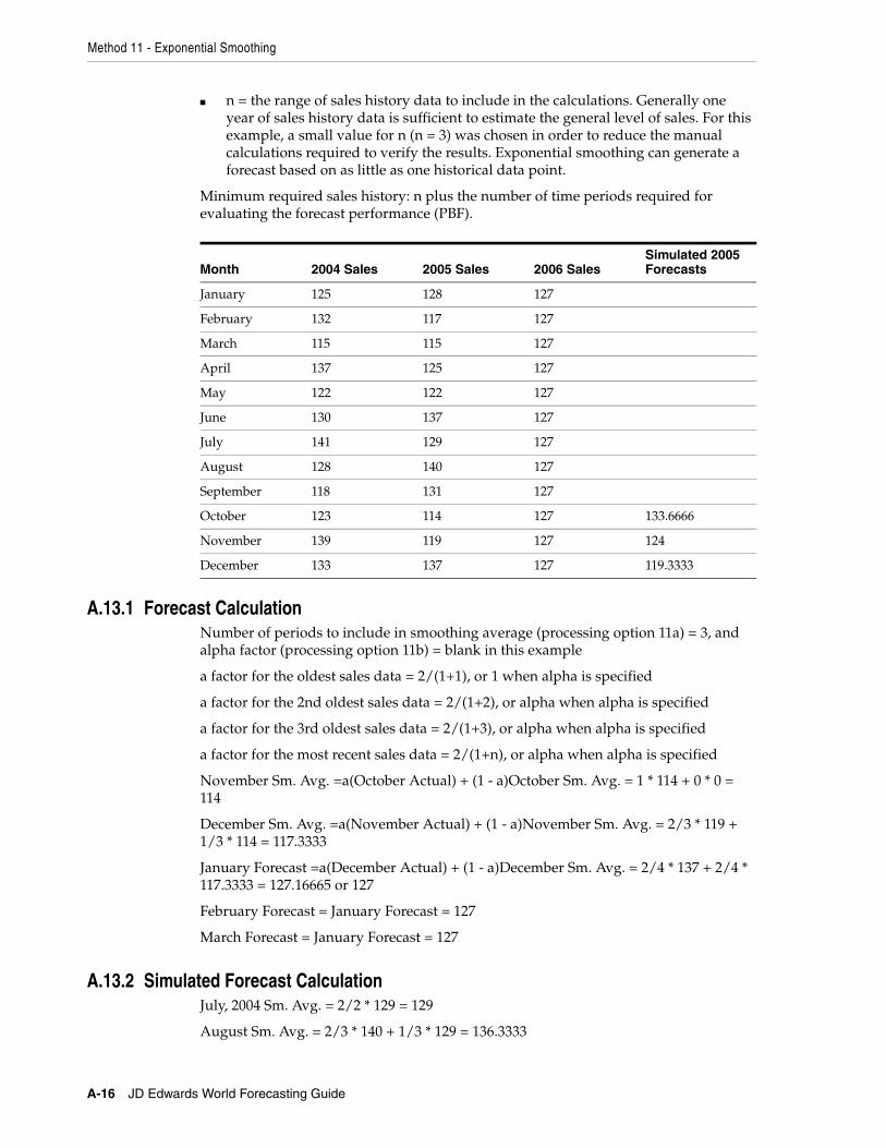
Method 11 - Exponential Smoothing
A-16 JD Edwards World Forecasting Guide
■ n = the range of sales history data to include in the calculations. Generally one year of sales history data is sufficient to estimate the general level of sales. For this example, a small value for n (n = 3) was chosen in order to reduce the manual calculations required to verify the results. Exponential smoothing can generate a forecast based on as little as one historical data point.
Minimum required sales history: n plus the number of time periods required for evaluating the forecast performance (PBF).
A.13.1 Forecast CalculationNumber of periods to include in smoothing average (processing option 11a) = 3, and alpha factor (processing option 11b) = blank in this example
a factor for the oldest sales data = 2/(1+1), or 1 when alpha is specified
a factor for the 2nd oldest sales data = 2/(1+2), or alpha when alpha is specified
a factor for the 3rd oldest sales data = 2/(1+3), or alpha when alpha is specified
a factor for the most recent sales data = 2/(1+n), or alpha when alpha is specified
November Sm. Avg. =a(October Actual) + (1 - a)October Sm. Avg. = 1 * 114 + 0 * 0 = 114
December Sm. Avg. =a(November Actual) + (1 - a)November Sm. Avg. = 2/3 * 119 + 1/3 * 114 = 117.3333
January Forecast =a(December Actual) + (1 - a)December Sm. Avg. = 2/4 * 137 + 2/4 * 117.3333 = 127.16665 or 127
February Forecast = January Forecast = 127
March Forecast = January Forecast = 127
A.13.2 Simulated Forecast CalculationJuly, 2004 Sm. Avg. = 2/2 * 129 = 129
August Sm. Avg. = 2/3 * 140 + 1/3 * 129 = 136.3333
Month 2004 Sales 2005 Sales 2006 SalesSimulated 2005 Forecasts
January 125 128 127
February 132 117 127
March 115 115 127
April 137 125 127
May 122 122 127
June 130 137 127
July 141 129 127
August 128 140 127
September 118 131 127
October 123 114 127 133.6666
November 139 119 127 124
December 133 137 127 119.3333

Method 12 - Exponential Smoothing with Trend and Seasonality
Forecast Calculation Examples A-17
September Sm. Avg. = 2/4 * 131 + 2/4 * 136.3333 = 133.6666
October, 2004 sales = Sep Sm. Avg. = 133.6666
August, 2004 Sm. Avg. = 2/2 * 140 = 140
September Sm. Avg. = 2/3 * 131 + 1/3 * 140 = 134
October Sm. Avg. = 2/4 * 114 + 2/4 * 134 = 124
November, 2004 sales = Sep Sm. Avg. = 124
September 2004 Sm. Avg. = 2/2 * 131 = 131
October Sm. Avg. = 2/3 * 114 + 1/3 * 131 = 119.6666
November Sm. Avg. = 2/4 * 119 + 2/4 * 119.6666 = 119.3333
December 2004 sales = Sep Sm. Avg. = 119.3333
A.13.3 Percent of Accuracy CalculationPOA = (133.6666 + 124 + 119.3333) / (114 + 119 + 137) * 100 = 101.891
A.13.4 Mean Absolute Deviation CalculationMAD = (|133.6666 - 114| + |124 - 119| + |119.3333 - 137|) / 3 = 14.1111
A.14 Method 12 - Exponential Smoothing with Trend and SeasonalityThis method is similar to Method 11, Exponential Smoothing in that a smoothed average is calculated. However, Method 12 also includes a term in the forecasting equation to calculate a smoothed trend. The forecast is composed of a smoothed averaged adjusted for a linear trend. When specified in the processing option, the forecast is also adjusted for seasonality.
Forecast specifications:
■ a = the smoothing constant used in calculating the smoothed average for the general level or magnitude of sales. Valid values for alpha range from 0 to 1.
■ b = the smoothing constant used in calculating the smoothed average for the trend component of the forecast. Valid values for beta range from 0 to 1.
■ Whether a seasonal index is applied to the forecast
Minimum required sales history: two years plus the number of time periods required for evaluating the forecast performance (PBF).
Method 12 uses two exponential smoothing equations and one simple average to calculate a smoothed average, a smoothed trend, and a simple average seasonal factor.
A.14.1 Forecast CalculationA) An exponentially smoothed average
Note: a and b are independent of each other. They do not have to add to 1.0.
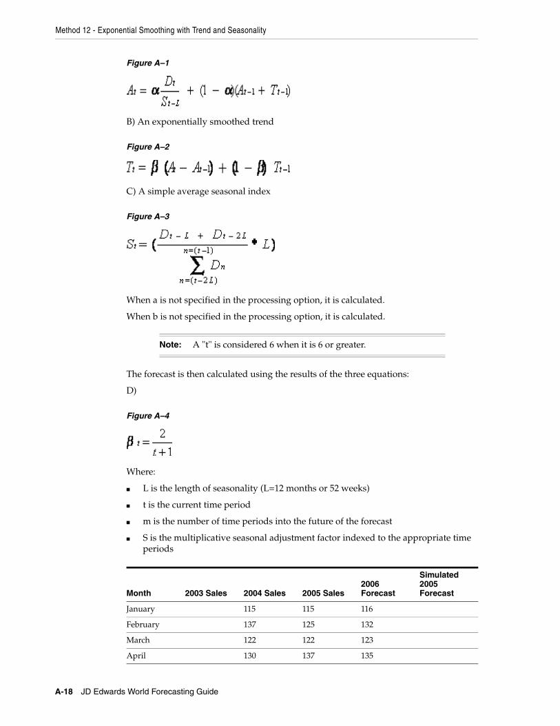
Method 12 - Exponential Smoothing with Trend and Seasonality
A-18 JD Edwards World Forecasting Guide
Figure A–1
B) An exponentially smoothed trend
Figure A–2
C) A simple average seasonal index
Figure A–3
When a is not specified in the processing option, it is calculated.
When b is not specified in the processing option, it is calculated.
The forecast is then calculated using the results of the three equations:
D)
Figure A–4
Where:
■ L is the length of seasonality (L=12 months or 52 weeks)
■ t is the current time period
■ m is the number of time periods into the future of the forecast
■ S is the multiplicative seasonal adjustment factor indexed to the appropriate time periods
Note: A "t" is considered 6 when it is 6 or greater.
Month 2003 Sales 2004 Sales 2005 Sales2006 Forecast
Simulated 2005 Forecast
January 115 115 116
February 137 125 132
March 122 122 123
April 130 137 135

Method 12 - Exponential Smoothing with Trend and Seasonality
Forecast Calculation Examples A-19
A.14.2 Forecast CalculationAlpha, and beta factor (processing option 12a, and 12b) = blank, and seasonality (processing option 13c) is '1' in this example
May 141 129 137
June 128 140 136
July 118 131 127
August 118 123 114 121 122.81
September 121 139 119 132 133.14
October 130 133 137 139 135.33
November 1543 1514
December
Total
Description Calculation
January, 05 Seasonal Index, S1
= (125 + 128)/(1543 + 1514) * 12
= 0.99313
January, 05 Smoothed Average, A1
= Jan, 05 Actual/Jan, 05 Seasonal Index
= 128/0.99313
= 128.885
January, 05 Smoothed Trend, T1
= 0 insufficient information to calculate first smoothed trend
February Seasonal Index, S2 =(132 + 117)/(1543 + 1514) * 12
= 0.97742
February Smoothed Average, A2
= 122.7519
February Smoothed Trend, T2
= 2/3 * (122.7519 - 128.885) + 1/3 * 0
= -4.0887333
March Seasonal Index, S3 = (115 + 115)/3057 * 12 = 0.90284
March Smoothed Average, A3
= 2/4 * 115/0.90284 + 2/4 * [122.7519 + (-4.088733)] = 123.01950
March Smoothed Trend, T3 = 2/4 (123.01950 - 122.7519) + 2/4 (-4.0888733) = -1.91063665
(Continued through December '06)
December '06 Seasonal Index, S12
= (133 + 137)/3057 * 12 = 1.05986
December Smoothed Average, A12
= (2/13)137/1.05986 + (11/13)(A11 + T11) = 19.8865 + 107.47247 = 127.35897
Month 2003 Sales 2004 Sales 2005 Sales2006 Forecast
Simulated 2005 Forecast

Evaluating the Forecasts
A-20 JD Edwards World Forecasting Guide
Calculation of Linear and Seasonal Exponentially Smoothed Forecast
January '06 = (A12+T12)S1 = (127.35897 + 0.28814 * 1) * 0.99313 = 126.77 or 127
February '06 = (A12+T12)S2 = (127.35897 + 0.28814 * 2 ) * 0.9774 = 125.04 or 125
March '06 = (A12+T12)S3 = (127.35897 + 0.28814 * 3) * 0.902845 = 115.77 or 116
December '06 = (A12+T12)S12 = (127.35897 + 0.28814 * 12) * 1.059862 = 138.65 or 139
A.14.3 Simulated Forecast Calculation
October 2005 sales = (A12 + T12*1)S1 = (129.1410 + 0.6343542 * 1) * 0.94633 = 129.775379872 * 0.94633 = 122.81
November 2005 sales = (A12 + T12*2)S2 = (129.1410 + 0.6343542 * 2) * 1.02094236 = 133.14
December 2005 sales = (A12 + T12*3)S3 = (129.1410 + 0.6343542 * 3) * 1.032722508 = 135.33
A.14.4 Percent of Accuracy CalculationPOA = (122.81 + 133.14 + 135.33) / (114 + 119 + 137) * 100 = 105.75
A.14.5 Mean Absolute Deviation CalculationMAD = (|122.81 - 114| + |133.14 - 119| + |135.33 - 137|) / 3 = 8.2
A.15 Evaluating the ForecastsYou can select forecasting methods to generate as many as twelve forecasts for each product. Each forecasting method will probably create a slightly different projection. When thousands of products are forecast, it is impractical to make a subjective decision regarding which of the forecasts to use in your plans for each of the products.
Description Calculation
October, 04 Seasonal Index, S1
= (118 + 123)/(3056) * 12
= 0.94633
October, 04 Smoothed Average, A1
=a * Oct, 04 Actual/Oct, 04 Seasonal Index
= 123/0.94633
= 129.9758
October, 04 Smoothed Trend, T1
= 0 insufficient information to calculate first smoothed trend
(Continued through September '05)
September, 05 Seasonal Index, S12
= (118 + 131)/(3056) * 12
= 0.97774869
September, 05 Smoothed Average, A12
= 2/13*131/0.97774869 + 11/13*(A11 + T11)
= 129.1410
September, 05 Smoothed Trend, T12
= 2/7 * (129.141025630 - A11) + 5/7 * T11 = 0.6343542

Mean Absolute Deviation (MAD)
Forecast Calculation Examples A-21
The system automatically evaluates performance for each of the forecasting methods that you select, and for each of the products forecast. You can choose between two performance criteria, Mean Absolute Deviation (MAD) and Percent of Accuracy (POA). MAD is a measure of forecast error. POA is a measure of forecast bias. Both of these performance evaluation techniques require actual sales history data for a user specified period of time. This period of recent history is called a "holdout period" or "periods best fit" (PBF).
To measure the performance of a forecasting method, use the forecast formulae to simulate a forecast for the historical holdout period. There will usually be differences between actual sales data and the simulated forecast for the holdout period.
When multiple forecast methods are selected, this same process occurs for each method. Multiple forecasts are calculated for the holdout period, and compared to the known sales history for that same period of time. The forecasting method producing the best match (best fit) between the forecast and the actual sales during the holdout period is recommended for use in your plans. This recommendation is specific to each product, and might change from one forecast generation to the next.
A.16 Mean Absolute Deviation (MAD)MAD is the mean (or average) of the absolute values (or magnitude) of the deviations (or errors) between actual and forecast data. MAD is a measure of the average magnitude of errors to expect, given a forecasting method and data history. Because absolute values are used in the calculation, positive errors do not cancel out negative errors. When comparing several forecasting methods, the one with the smallest MAD has shown to be the most reliable for that product for that holdout period. When the forecast is unbiased and errors are normally distributed, there is a simple mathematical relationship between MAD and two other common measures of distribution, standard deviation and Mean Squared Error:
A.16.1 Percent of Accuracy (POA)Percent of Accuracy (POA) is a measure of forecast bias. When forecasts are consistently too high, inventories accumulate and inventory costs rise. When forecasts are consistently two low, inventories are consumed and customer service declines. A forecast that is 10 units too low, then 8 units too high, then 2 units too high, would be an unbiased forecast. The positive error of 10 is canceled by negative errors of 8 and 2.
Error = Actual - Forecast
When a product can be stored in inventory, and when the forecast is unbiased, a small amount of safety stock can be used to buffer the errors. In this situation, it is not so important to eliminate forecast errors as it is to generate unbiased forecasts. However in service industries, the above situation would be viewed as three errors. The service would be understaffed in the first period, then overstaffed for the next two periods. In services, the magnitude of forecast errors is usually more important than is forecast bias.
Figure A–5

Mean Absolute Deviation (MAD)
A-22 JD Edwards World Forecasting Guide
Note: The summation over the holdout period allows positive errors to cancel negative errors. When the total of actual sales exceeds the total of forecast sales, the ratio is greater than 100%. Of course, it is impossible to be more than 100% accurate. When a forecast is unbiased, the POA ratio will be 100%. Therefore, it is more desirable to be 95% accurate than to be 110% accurate. The POA criteria select the forecasting method that has a POA ratio closest to 100%.

B
Functional Servers B-1
BFunctional Servers
This appendix contains the topic:
■ Section B.1, "About Functional Servers."
B.1 About Functional ServersSeveral JD Edwards World programs access functional servers. The purpose of functional servers is to provide a central location for standard business rules about entering documents, such as vouchers, invoices, and journal entries. These business rules establish the following:
■ Data dictionary default values
■ Field edits and valid values
■ Error processing
■ Relationships between fields or applications
The advantages of a functional server are:
■ It reduces maintenance of entry programs because edit rules reside in one central location.
■ You can standardize documents across all applications because you create them using the same business rules.
■ Generally, the user interface (appearance and interaction) of a form is now separate from how a program works.
To set up business rules for an entry programThe steps for setting up business rules for an entry program are:
1. Create a DREAM Writer version for a specific functional server program (for example, XT0411Z1 for voucher entry).
2. Set the processing options within the version according to your company requirements.
3. Specify the version you want the entry program to use in the processing options for that entry program.
You can have all your entry programs use the same DREAM Writer version (and thus, use the same rules) or you can set up different DREAM Writer versions. JD Edwards World provides DREAM Writer version ZJDE0001 as the default functional server version for your entry programs.

About Functional Servers
B-2 JD Edwards World Forecasting Guide
Example: Voucher Processing Functional ServerThe following programs use the voucher processing functional server. JD Edwards World provides two demo versions of the functional server, ZJDE0001 and ZJDE0002.
■ Speed Voucher Entry (P040015)
■ Standard Voucher Entry (P04105)
■ Void Payment Entry (P4704103)
■ Credit Tied to Debit Bill (P041010)
■ Multi-Voucher (P041017)
■ Calculate Withholding (P04580)
Caution: Only the person responsible for system-wide setup should make changes to the functional server version. For more information about how to set up DREAM Writer versions, see the JD Edwards World Technical Foundation Guide.

Index-1
Index
Numerics52 period date pattern
setting up, 3-5
AAbout detail forecasts, 2-1About planning bill forecasts, 14-1About summary forecasts, 6-1, 11-1Address book records
revising, 7-5
BBranch/plant data
reviewing, 7-6Business Units by Company form (P0006A), 7-7
CCategory Codes form (P010512), 7-6Company hierarchy
example, 6-2hierarchy of company 100, 6-4summary codes, 6-4
Comparing summaries of detail forecasts and summary forecasts
See Defining the distribution hierarchy (P4091)Considerations, 1-10Copying sales order history, 4-1
before you begin, 4-2See Setting up detail forecasts
Copying summary sales order history, 12-1before you begin, 12-3See Setting up detail forecastsSee Setting up summary forecasts
DDate Pattern Revisions form (P0008), 3-4Defining the distribution hierarchy, 7-1
before you begin, 7-3Demand patterns, 1-8Detail forecasts
generating, 5-1generating summaries, 8-1
reviewing, 5-2revising, 5-4setting up, 3-1working with, 5-1
Distribution hierarchydefining, 7-1
EEnter/Change Actuals form (P3460), 4-3Enter/Change Bill (P3002)
fold area, 15-5Enter/Change Bill form (P3002), 15-5Enter/Change Summaries form (P34200), 9-1, 9-4,
12-3Entering a planning bill, 15-5Examples
company hierarchy, 6-2distribution hierarchy for company 100, 7-2exploding the forecast to the item level, 14-3planning bill forecasts, pseudo parent item, 14-1reviewing and revising sales order history, 4-2using the Force Changes program, 9-7
Exploding the forecast to the item level, 14-2
FFeatures
demand patterns, 1-8forecast accuracy, 1-9forecasting, 1-4
Fiscal date patternsetting up, 3-3
Forecast accuracystatistical laws, 1-9
Forecast considerations, 1-10See Appendix A - Forecast calculation examples
Forecast Summary Detail form (P34200W), 9-2Forecast Summary Revisions (P3400)
fold area, 9-5Forecast Summary Revisions form (P3400), 9-4Forecast Text form (P0016), 5-6Forecast types
setting up, 3-6Forecast Types form (P00051), 3-6Forecasting

Index-2
features, 1-4Forecasting level and methods, 1-5Forecasting overview, 1-1Forecasting process, 1-10Forms
Business Units by Company, 7-7Category Codes, 7-6Date Pattern Revisions, 3-4Enter/Change Actuals, 4-3Enter/Change Bill, 15-5Enter/Change Summaries, 9-1, 9-4, 12-3Forecast Summary Detail, 9-2Forecast Summary Revisions, 9-4Forecast Text, 5-6Forecast Types, 3-6General User Defined Codes, 6-5Item Branch Class Codes, 7-9, 15-3Item Branch Information, 15-2Item Branch/Plant Information, 7-9Item Master Information, 15-1Multi Level Bill Inquiry, 15-6Plant Manufacturing Data, 15-2Review Forecast, 5-2Set 52 Period Date, 3-6Summary Codes, 7-3Summary Constants, 7-3Supply/Demand Inclusion Rules, 3-2
GGeneral User Defined Codes form (P00051), 6-5Generating detail forecasts, 5-1Generating planning bill forecasts, 16-1
before you begin, 16-1See Entering a planning bill
Generating summaries of detail forecasts, 8-1before you begin, 8-2
Generating summary forecasts, 13-1before you begin, 13-2
Graphiccompany hierarchy, 6-2Force Changes program, 9-7generate summary forecast, 13-2summary forecast, 13-1
IItem Branch Class Codes form (P41025), 7-9, 15-3Item Branch Information form (P41026), 15-2Item Branch/Plant Information form (P41026), 7-9Item location records
reviewing, 7-8Item master information
planning bill, 15-1Item Master Information form (P4101), 15-1Items from summary constants, 8-2
LLevels and methods, 1-5
best fit, 1-5
calculated percent over last year, 1-6exponential smoothing, 1-8flexible method, 1-7geometrically weighted moving average, 1-8last year to this year, 1-7linear approximation, 1-7methods, 1-6moving average, 1-7percent over last year, 1-6second degree approximation, 1-7weighted moving average, 1-8
MMenu
overview, 1-12Multi Level Bill Inquiry form (P30200), 15-6
OOverview
forecasting, 1-1revising summaries of forecasts, 9-1system integration, 1-2
PPlanning bill
entering, 15-5item master information, 15-1setting up, 15-1
Planning bill forecastsexploding the forecast to the item level, 14-2generating, 16-1
Plant Manufacturing Data form (P41027), 15-2Processing options
Summary Forecast Generation, 13-2Programs and IDs
P00051 (forecast types), 3-6P00051 (general user defined codes), 6-5P00051 (summary codes), 7-3P0006A (business units by company), 7-7P0008 (date pattern revisions), 3-4P0008B (set 52 period date), 3-6P0016 (forecast text), 5-6P010512 (category codes), 7-6P3002 (enter/change bill), 15-5P30200 (multi level bill inquiry), 15-6P3400 (forecast summary revisions), 9-4P34004 (supply/demand inclusion rules), 3-2P34200 (enter/change summaries), 9-1, 9-4, 12-3P34200W (forecast summary detail), 9-2P34201 (review forecast), 5-2P3460 (enter/change sales order history), 4-3P4091 (summary constants), 7-3P4101 (item master information), 15-1P41025 (item branch class codes), 7-9, 15-3P41026 (item branch information), 15-2P41026 (item branch/plant information), 7-9P41027 (plant manufacturing data), 15-2

Index-3
RRecords for large customers, 4-2Review Forecast form (P34201), 5-2Reviewing and revising sales order history, 4-2Reviewing and revising summary sales order
history, 12-3before you begin, 12-3
Reviewing branch/plant data, 7-6before you begin, 7-7
Reviewing item location records, 7-8See Defining the distribution hierarchy (P4091)
Reviewing the summary forecast, 9-1Revising address book records, 7-5
before you begin, 7-5Revising detail forecasts, 5-4Revising summaries of forecasts, 9-1
before you begin, 9-1See Generating summaries of detail forecastsSee Generating summary forecasts
Revising summary forecasts using the Force Change program, 9-7
before you begin, 9-8Revising the summary forecast, 9-3
See Revising summary forecasts using the Force Change program
SSales order history
copying, 4-1reviewing and revising, 4-2working with, 4-1
Set 52 Period Date form (P0008B), 3-6Setting the revised flag processing option, 9-8Setting up a planning bill, 15-1Setting up detail forecasts, 3-1Setting up fiscal date patterns, 3-3Setting up forecast types, 3-6Setting up item master information, 15-1Setting up summary forecasts, 7-1
before you begin, 7-1See Setting up detail forecastsSee Summary forecasts
Setting up supply/demand inclusion rules, 3-1Setting up the 52 period date pattern, 3-5Specifying bypassed records, 9-8Statistical laws
forecast accuracy, 1-9Summaries
comparing detail and summary forecasts, 6-2, 11-1
Summary Codes form (P00051), 7-3Summary Constants form (P4091)Summary Constants
form (P4091), 7-3Summary Forecast Generation
processing options, 13-2Summary forecasts, 6-1
generating, 13-1reviewing, 9-1revising, 9-3
revising with the Force Changes program, 9-7setting up, 7-1
Summary sales order historycopying, 12-1records for large customers, 4-2reviewing and revising, 12-3working with, 12-1
Supply/demand inclusion rulessetting up for forecasting, 3-1
Supply/Demand Inclusion Rules form (P34004), 3-2System integration, 1-2
distribution resources planning, 1-4master production schedule, 1-4material requirements planning, 1-4resource requirements planning, 1-4
TTables
Address Book, 1-12Branch/Plant Master, 1-12Business Unit Master, 1-12Detail Forecast, 1-12Fast Path Command, 1-13Forecast Summary Work, 1-12Item Master, 1-12Sales History, 1-12Sales Order Detail, 1-12Summary Constants, 1-12Summary Forecast, 1-12
UUDC
forecast type, 3-6Unit of measure, 12-3
WWorking with detail forecasts, 5-1Working with sales order history, 4-1Working with summary sales order history, 12-1

Index-4