Forecast based on different data types: A before and after ...Fax: 01-633 10 57...
47
Forecast based on different data types: A before and after study (Revealed Preference) M Vrtic Travel Survey Metadata Series 3
Transcript of Forecast based on different data types: A before and after ...Fax: 01-633 10 57...
Forecast based on different data types: A before and after study (Revealed Preference)
M Vrtic
Travel Survey Metadata Series 3

Travel Survey Metadata Series
Forecast based on different data types: A before and after study (Revealed Preference) M Vrtic IVT ETH Zürich Zürich Phone: 01-633 31 07 Fax: 01-633 10 57 [email protected]
Abstract
In addition to adequate data, the formulation of transport forecasts relies upon a knowledge of the relationships between the demand for transport and those factors which influence it. These relationships are described with mathematical functions and the their model parameters. The parameters derived from revealed preference (RP) data are often subject to too many impon-derables and are thus of only limited value in many cases. The main cause of this uncertainty is data which is either insufficiently detailed or unsuitable for estimating transport demand functions. For this reason, an earlier SVI study concerning the sensitivity of passenger transport to sup-ply- side and price changes recommended that research should be conducted in parallel with major transport infrastructure investments. In this way this recommended project would be able to check and validate the quality of the findings from alternative or supplementary stated preference (SP) (Vrtic et al., 2000), as both forecast and actual changes in demand would be known to it. The launch of intercity tilting-trains (known as ICNs) in 2001 and further supply-side im-provements to road and rail transport supply offered an opportunity to conduct ex ante/ex post surveys in order to verify the forecasting approaches in a defined period. This mix of qualita-tive and quantitative changes is a particular challenge for forecasting and the attendant data collection process. Nonetheless, it is a challenge that must be overcome again and again in day-to-day practice. As the supply-side changes are generally small, it was expected that changes on the demand side will be concentrated at the level of mode and route choice. The principal aim of this research remit was to verify and identify the limits and possibilities of the three data sources for forecasting by means of an ex ante/ex post analysis. However, this study also offered an opportunity to analyse other aspects of importance to transport fore-casting. Here, in addition to the study methodology, the quality and accessibility of the avail-able bodies of data proved to be crucial factors in modelling transport movements and events. In a first stage the study estimated a detailed public transport route choice model and cali-brated national network models for both road and rail demand. This is an essential preliminary stage to the calculation of modal shifts in demand for transport and the subsequent review of the different forecasts. In the case of mode choice changes, the three most common ap-proaches to forecasting were to be tested: • Direct elasticity, known from previous studies • RP models, i.e. model parameters based on RP data • SP models, i.e. model parameters based on SP data The primary benefits of this study can be summarized as follows: - It sets out the opportunities and limits, as well as the advantages and disadvan-tages, of the three data sources for forecasting under review. - This the first study to provide models of route and mode choice which have been estimated from SP data. The model parameters estimated using this data provide the basis for the practical application of
Forecast based on different data types: A before and after study (Revealed Preference)___________________May 2004
i
mode and route choice models following supply-side transport changes. - The estimated model parameters, current figures and the relative valuations dem-onstrate the importance of individual variables to mode and route choice. They were estimated for each trip purpose. - The study showed that in this case the forecasts derived from the SP-data were more consistent and more precise than either the estimates from the direct elastic-ities or the RP data. - Verifying transport forecasts shows how and where further improvements can or must still be made with regard to both data bases and methodology. - The study describes the possibilities and methodical foundation for common SP/RP estimates of model parameters.
Keywords
Route and mode choice
Preferred citation style
Vrtic, M. (2004) Forecast based on different data types: A before and after study (Revealed Preference) , Travel Survey Metadata Series, 3, Institute for Transport Planning and Systems (IVT); ETH Zürich, Zürich.
ii

1.0 Document Description Citation
Title: Forecast based on different data types: A before and after study (Revealed Preference )
Identification Number: KEP RP
Authoring Entity: Institute for Transport Plannig and Systems (IVT) (ETH Zurich)
Other identifications and acknowledgements:
Vtric M.
Producer: Vtric M.
Copyright: Institute for Transport Plannig and Systems (IVT)
Date of Production: 2003-06-17
Software used in Production: Nesstar Publisher
Forecast based on different data types: A before and after study (Revealed Preference)_____________May 2004
1
2.0 Study Description Citation
Title: Forecast based on different data types: A before and after study (Revealed Preference)
Identification Number: KEP RP
Authoring Entity: Mr. M. Vrtic (Institute for Transport Planning and Systems, ETH Zurich)
Prof. KW Axhausen (Institute for Transport Planning and Systems, ETH Zurich)
Producer: Mr. M. Vrtic
Prof. KW Axhausen
Date of Production: 2003-06-17
Software used in Production: Nesstar Publisher
Funding Agency/Sponsor: Federal Office for Spatial Development
Funding Agency/Sponsor: Swiss Federal Railway
Grant Number: ARE, Bern
Grant Number: SBB, Bern
Distributor: Federal Office for Spatial Development
Distributor: Swiss Federal Railway
Forecast based on different data types: A before and after study (Revealed Preference)_____________May 2004
2
Study Scope
Keywords: Route and mode choice , Stated preference , Revealed preference , Public transport , Tilting trains , Instituute for Transport Planning and Systems
Topic Classification: Revealed prefernce , Stated preference
Abstract:
In addition to adequate data, the formulation of transport forecasts relies upon a knowledge of the relationships between the demand for transport and those factors which influence it. These relationships are described with mathematical functions and the their model parameters. The parameters derived from revealed preference (RP) data are often subject to too many impon-derables and are thus of only limited value in many cases. The main cause of this uncertainty is data which is either insufficiently detailed or unsuitable for estimating transport demand functions. For this reason, an earlier SVI study concerning the sensitivity of passenger transport to sup-ply- side and price changes recommended that research should be conducted in parallel with major transport infrastructure investments. In this way this recommended project would be able to check and validate the quality of the findings from alternative or supplementary stated preference (SP) (Vrtic et al., 2000), as both forecast and actual changes in demand would be known to it. The launch of intercity tilting-trains (known as ICNs) in 2001 and further supply-side im-provements to road and rail transport supply offered an opportunity to conduct ex ante/ex post surveys in order to verify the forecasting approaches in a defined period. This mix of qualita-tive and quantitative changes is a particular challenge for forecasting and the attendant data collection process. Nonetheless, it is a challenge that must be overcome again and again in day-to-day practice. As the supply-side changes are generally small, it was expected that changes on the demand side will be concentrated at the level of mode and route choice. The principal aim of this research remit was to verify and identify the limits and possibilities of the three data sources for forecasting by means of an ex ante/ex post analysis. However, this study also offered an opportunity to analyse other aspects of importance to transport fore-casting. Here, in addition to the study methodology, the quality and accessibility of the avail-able bodies of data proved to be crucial factors in modelling transport movements and events. In a first stage the study estimated a detailed public transport route choice model and cali-brated national network models for both road and rail demand. This is an essential preliminary stage to the calculation of modal shifts in demand for transport and the subsequent review of the different forecasts. In the case of mode choice changes, the three most common ap-proaches to forecasting were to be tested: • Direct elasticity, known from previous studies •
Forecast based on different data types: A before and after study (Revealed Preference)_____________May 2004
3

RP models, i.e. model parameters based on RP data • SP models, i.e. model parameters based on SP data The primary benefits of this study can be summarized as follows: - It sets out the opportunities and limits, as well as the advantages and disadvan-tages, of the three data sources for forecasting under review. - This the first study to provide models of route and mode choice which have been estimated from SP data. The model parameters estimated using this data provide the basis for the practical application of mode and route choice models following supply-side transport changes. - The estimated model parameters, current figures and the relative valuations dem-onstrate the importance of individual variables to mode and route choice. They were estimated for each trip purpose. - The study showed that in this case the forecasts derived from the SP-data were more consistent and more precise than either the estimates from the direct elastic-ities or the RP data. - Verifying transport forecasts shows how and where further improvements can or must still be made with regard to both data bases and methodology. - The study describes the possibilities and methodical foundation for common SP/RP estimates of model parameters.
Country: Switzerland
Geographic Coverage: Switzerland
Unit of Analysis: Person
Universe: All the individuals permanantly residing in Switzerland.
Forecast based on different data types: A before and after study (Revealed Preference)_____________May 2004
4

Methodology and Processing Time Method: 9 months (January 2001 to September 2001)
Sampling Procedure:
Sample frame: All the individuals of age 15-84, residing permanantly in Switzerland Sample unit: Person or Individual Sampling technique: Random sampling
Mode of Data Collection:
Self-Administrative and structured written interview technique was implemented.
Forecast based on different data types: A before and after study (Revealed Preference)_____________May 2004
5

Sources Statement Weighting: No weighting was done.
Forecast based on different data types: A before and after study (Revealed Preference)_____________May 2004
6

Other Study Description Materials Related Materials
Citation Title: Revealed preference questioannaire
Holdings Information: www.ivt.baug.ethz.ch/ethtda/kep/rp/questioannaire.pdf
Forecast based on different data types: A before and after study (Revealed Preference)_____________May 2004
7

3.0 File Description File: Revealed Preference.NSDstat
Number of cases: 46051
No. of variables per record: 24
Type of File: NSDstat 200203
Forecast based on different data types: A before and after study (Revealed Preference)_____________May 2004
8
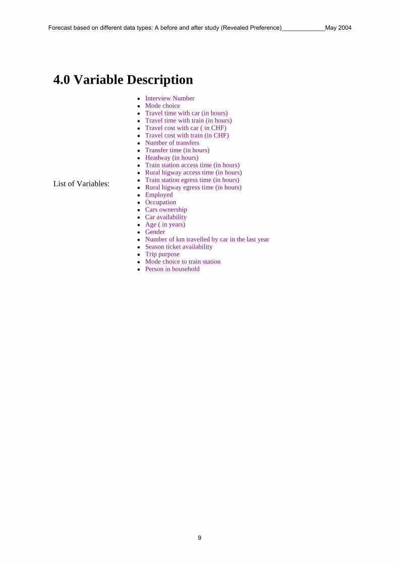
4.0 Variable Description
List of Variables:
Interview Number Mode choice Travel time with car (in hours) Travel time with train (in hours) Travel cost with car ( in CHF) Travel cost with train (in CHF) Number of transfers Transfer time (in hours) Headway (in hours) Train station access time (in hours) Rural higway access time (in hours) Train station egress time (in hours) Rural higway egress time (in hours) Employed Occupation Cars ownership Car availability Age ( in years) Gender Number of km travelled by car in the last year Season ticket availability Trip purpose Mode choice to train station Person in household
Forecast based on different data types: A before and after study (Revealed Preference)_____________May 2004
9

Variables
Forecast based on different data types: A before and after study (Revealed Preference)_____________May 2004
10

Variable: Interview Number
Location:
Width: 11
Range of Valid Data Values: 3 to 71569
Summary Statistics:
Variable Format: numeric
Forecast based on different data types: A before and after study (Revealed Preference)_____________May 2004
11

Variable: Mode choice
Location:
Width: 11
Range of Valid Data Values: 1 to 2
Total Responses: Summation of listed categories: 46051
Summary Statistics:
Minimum : 1
Maximum : 2
Mean : 1.224
Standard deviation : 0.417
Variable Format: numeric
Value Label Frequency
1 . Car 35748
2 . Train 10303
Forecast based on different data types: A before and after study (Revealed Preference)_____________May 2004
12
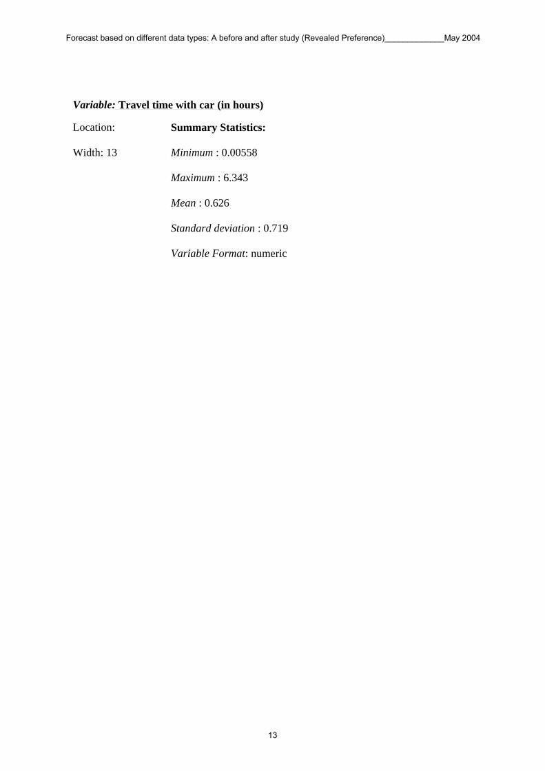
Variable: Travel time with car (in hours)
Location:
Width: 13
Summary Statistics:
Minimum : 0.00558
Maximum : 6.343
Mean : 0.626
Standard deviation : 0.719
Variable Format: numeric
Forecast based on different data types: A before and after study (Revealed Preference)_____________May 2004
13

Variable: Travel time with train (in hours)
Location:
Width: 13
Summary Statistics:
Minimum : 0
Maximum : 10.45
Mean : 0.804
Standard deviation : 0.972
Variable Format: numeric
Forecast based on different data types: A before and after study (Revealed Preference)_____________May 2004
14

Variable: Travel cost with car ( in CHF)
Location:
Width: 13
Summary Statistics:
Minimum : 0.0287
Maximum : 57.966
Mean : 4.86
Standard deviation : 6.556
Variable Format: numeric
Forecast based on different data types: A before and after study (Revealed Preference)_____________May 2004
15
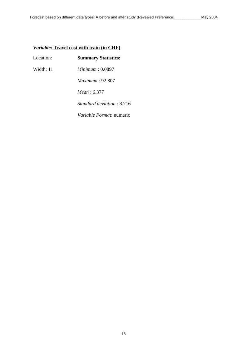
Variable: Travel cost with train (in CHF)
Location:
Width: 11
Summary Statistics:
Minimum : 0.0897
Maximum : 92.807
Mean : 6.377
Standard deviation : 8.716
Variable Format: numeric
Forecast based on different data types: A before and after study (Revealed Preference)_____________May 2004
16

Variable: Number of transfers
Location:
Width: 11
Summary Statistics:
Minimum : 0
Maximum : 4.2
Mean : 0.626
Standard deviation : 0.792
Variable Format: numeric
Forecast based on different data types: A before and after study (Revealed Preference)_____________May 2004
17

Variable: Transfer time (in hours)
Location:
Width: 11
Summary Statistics:
Minimum : 0
Maximum : 2.017
Mean : 0.108
Standard deviation : 0.18
Variable Format: numeric
Forecast based on different data types: A before and after study (Revealed Preference)_____________May 2004
18
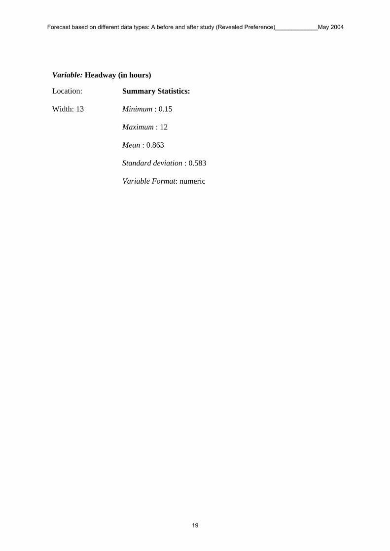
Variable: Headway (in hours)
Location:
Width: 13
Summary Statistics:
Minimum : 0.15
Maximum : 12
Mean : 0.863
Standard deviation : 0.583
Variable Format: numeric
Forecast based on different data types: A before and after study (Revealed Preference)_____________May 2004
19
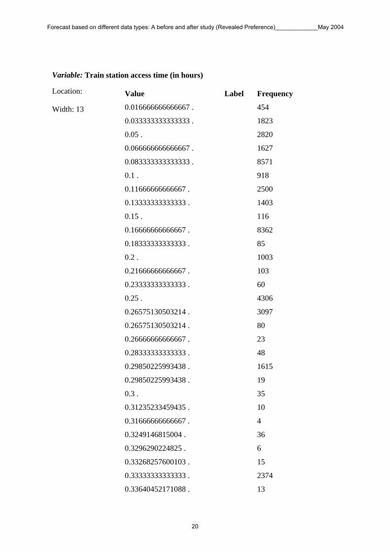
Variable: Train station access time (in hours)
Location:
Width: 13
Value Label Frequency
0.016666666666667 . 454
0.033333333333333 . 1823
0.05 . 2820
0.066666666666667 . 1627
0.083333333333333 . 8571
0.1 . 918
0.11666666666667 . 2500
0.13333333333333 . 1403
0.15 . 116
0.16666666666667 . 8362
0.18333333333333 . 85
0.2 . 1003
0.21666666666667 . 103
0.23333333333333 . 60
0.25 . 4306
0.26575130503214 . 3097
0.26575130503214 . 80
0.26666666666667 . 23
0.28333333333333 . 48
0.29850225993438 . 1615
0.29850225993438 . 19
0.3 . 35
0.31235233459435 . 10
0.31666666666667 . 4
0.3249146815004 . 36
0.3296290224825 . 6
0.33268257600103 . 15
0.33333333333333 . 2374
0.33640452171088 . 13
Forecast based on different data types: A before and after study (Revealed Preference)_____________May 2004
20
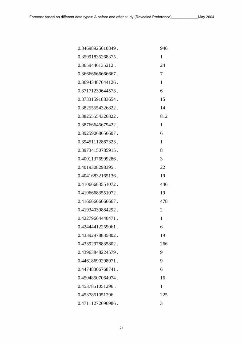
0.34698925610849 . 946
0.35991835268375 . 1
0.3659446135212 . 24
0.36666666666667 . 7
0.36943487044126 . 1
0.37171239644573 . 6
0.37331591883654 . 15
0.38255554326822 . 14
0.38255554326822 . 812
0.38766645679422 . 1
0.39259068656607 . 6
0.39451112867323 . 1
0.39734150785915 . 8
0.40011376999286 . 3
0.4019308298395 . 22
0.40416832165136 . 19
0.41066683551072 . 446
0.41066683551072 . 19
0.41666666666667 . 478
0.41934039884292 . 2
0.42279664440471 . 1
0.42444412259061 . 6
0.43392978835802 . 19
0.43392978835802 . 266
0.43963848224579 . 9
0.44618690298971 . 9
0.44748306768741 . 6
0.45048507064974 . 16
0.4537851051296 . 1
0.4537851051296 . 225
0.47111272696986 . 3
Forecast based on different data types: A before and after study (Revealed Preference)_____________May 2004
21
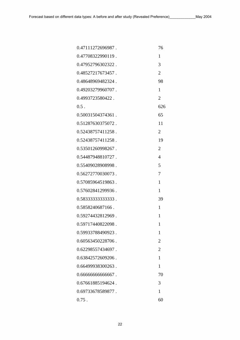
0.47111272696987 . 76
0.47708322990119 . 1
0.47952796302322 . 3
0.48527217673457 . 2
0.48648969482324 . 98
0.49203279960707 . 1
0.4993723580422 . 2
0.5 . 626
0.50031504374361 . 65
0.51287630375072 . 11
0.52438757411258 . 2
0.52438757411258 . 19
0.53501260998267 . 2
0.54487948810727 . 4
0.55409028908998 . 5
0.56272770030073 . 7
0.57085964519863 . 1
0.57602841299936 . 1
0.58333333333333 . 39
0.5858240687166 . 1
0.59274432812969 . 1
0.59717440822098 . 1
0.59933788490923 . 1
0.60563450228706 . 2
0.62298557434697 . 2
0.63842572609206 . 1
0.66499938300263 . 1
0.66666666666667 . 70
0.67661885194624 . 3
0.69733678589877 . 1
0.75 . 60
Forecast based on different data types: A before and after study (Revealed Preference)_____________May 2004
22

Total Responses: Summation of listed categories: 46051
Summary Statistics:
Minimum : 0.0167
Maximum : 2
Mean : 0.184
Standard deviation : 0.122
Variable Format: numeric
1 . 13
1.25 . 2
2 . 9
Forecast based on different data types: A before and after study (Revealed Preference)_____________May 2004
23

Variable: Rural higway access time (in hours)
Location:
Width: 13
Summary Statistics:
Minimum : 0.142
Maximum : 0.385
Mean : 0.159
Standard deviation : 0.0188
Variable Format: numeric
Forecast based on different data types: A before and after study (Revealed Preference)_____________May 2004
24
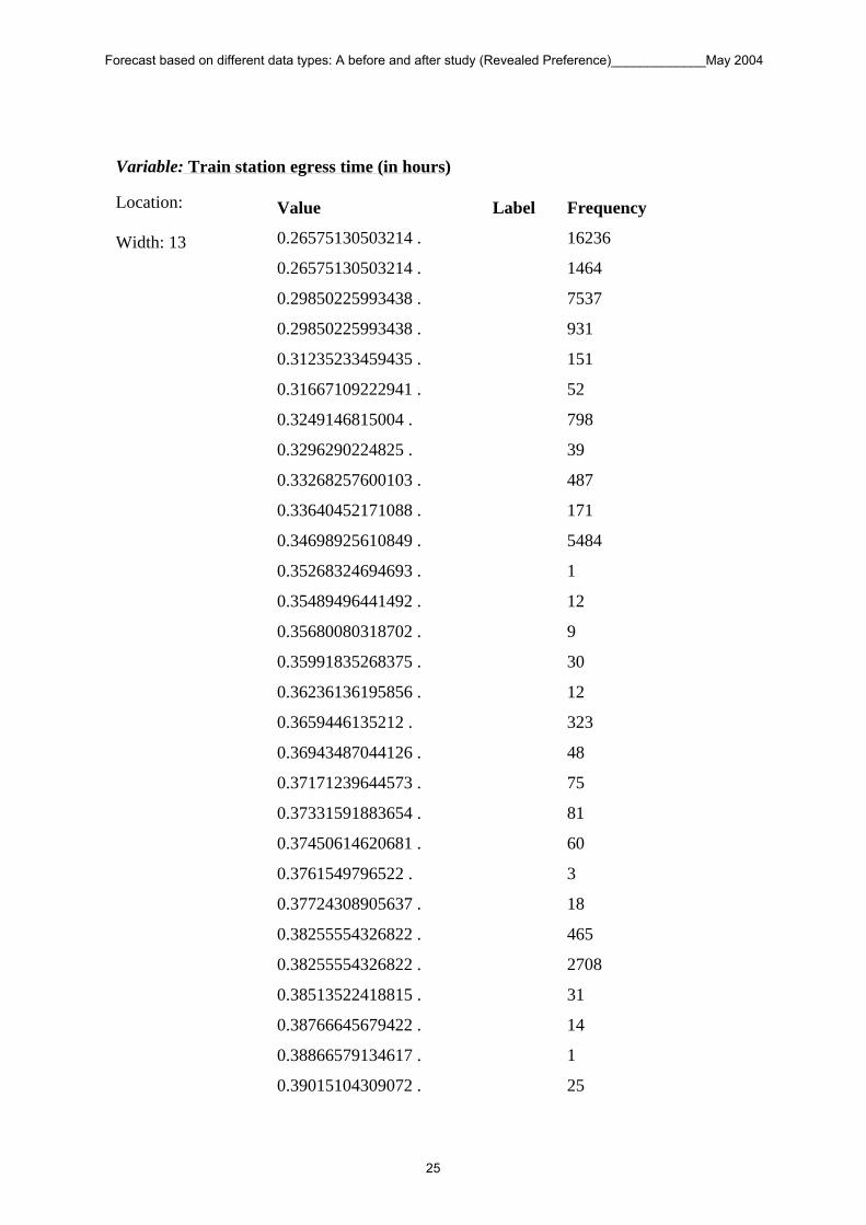
Variable: Train station egress time (in hours)
Location:
Width: 13
Value Label Frequency
0.26575130503214 . 16236
0.26575130503214 . 1464
0.29850225993438 . 7537
0.29850225993438 . 931
0.31235233459435 . 151
0.31667109222941 . 52
0.3249146815004 . 798
0.3296290224825 . 39
0.33268257600103 . 487
0.33640452171088 . 171
0.34698925610849 . 5484
0.35268324694693 . 1
0.35489496441492 . 12
0.35680080318702 . 9
0.35991835268375 . 30
0.36236136195856 . 12
0.3659446135212 . 323
0.36943487044126 . 48
0.37171239644573 . 75
0.37331591883654 . 81
0.37450614620681 . 60
0.3761549796522 . 3
0.37724308905637 . 18
0.38255554326822 . 465
0.38255554326822 . 2708
0.38513522418815 . 31
0.38766645679422 . 14
0.38866579134617 . 1
0.39015104309072 . 25
Forecast based on different data types: A before and after study (Revealed Preference)_____________May 2004
25

0.39259068656607 . 163
0.39451112867323 . 41
0.39734150785915 . 129
0.40011376999286 . 63
0.4019308298395 . 400
0.40416832165136 . 278
0.40549324989035 . 10
0.41066683551072 . 2553
0.41066683551072 . 195
0.41380265707602 . 15
0.41424475942405 . 6
0.41483199241859 . 5
0.41564986328399 . 7
0.41686748187798 . 29
0.41773055601585 . 14
0.41887283399313 . 21
0.41934039884292 . 29
0.42045601570985 . 2
0.42067047817729 . 1
0.42173772974405 . 1
0.42279664440471 . 48
0.42444412259061 . 97
0.42566672897345 . 4
0.42661008470083 . 33
0.42847734442949 . 2
0.43392978835802 . 190
0.43392978835802 . 962
0.43813945257221 . 24
0.43917180829978 . 35
0.43963848224579 . 34
0.44087517312796 . 26
Forecast based on different data types: A before and after study (Revealed Preference)_____________May 2004
26

0.44222267078712 . 8
0.44279610893152 . 1
0.444219219911 . 11
0.44618690298971 . 137
0.44748306768741 . 70
0.44908611537958 . 6
0.45048507064974 . 223
0.4537851051296 . 26
0.4537851051296 . 839
0.45545444841143 . 1
0.45639926358893 . 4
0.46078722703962 . 41
0.46148193568433 . 12
0.4627235723211 . 53
0.47111272696986 . 51
0.47111272696987 . 427
0.47708322990119 . 10
0.47791528977508 . 12
0.47952796302322 . 67
0.48054441118591 . 20
0.48071308841702 . 43
0.4815533736844 . 8
0.48354928242951 . 3
0.48527217673457 . 100
0.48648969482324 . 339
0.48648969482324 . 11
0.49125450364779 . 18
0.49158859950697 . 5
0.49203279960707 . 3
0.4993723580422 . 7
0.50031504374361 . 237
Forecast based on different data types: A before and after study (Revealed Preference)_____________May 2004
27
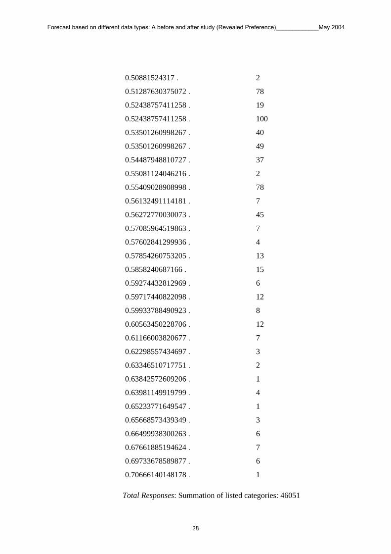
Total Responses: Summation of listed categories: 46051
0.50881524317 . 2
0.51287630375072 . 78
0.52438757411258 . 19
0.52438757411258 . 100
0.53501260998267 . 40
0.53501260998267 . 49
0.54487948810727 . 37
0.55081124046216 . 2
0.55409028908998 . 78
0.56132491114181 . 7
0.56272770030073 . 45
0.57085964519863 . 7
0.57602841299936 . 4
0.57854260753205 . 13
0.5858240687166 . 15
0.59274432812969 . 6
0.59717440822098 . 12
0.59933788490923 . 8
0.60563450228706 . 12
0.61166003820677 . 7
0.62298557434697 . 3
0.63346510717751 . 2
0.63842572609206 . 1
0.63981149919799 . 4
0.65233771649547 . 1
0.65668573439349 . 3
0.66499938300263 . 6
0.67661885194624 . 7
0.69733678589877 . 6
0.70666140148178 . 1
Forecast based on different data types: A before and after study (Revealed Preference)_____________May 2004
28

Summary Statistics:
Minimum : 0.266
Maximum : 0.707
Mean : 0.327
Standard deviation : 0.0683
Variable Format: numeric
Forecast based on different data types: A before and after study (Revealed Preference)_____________May 2004
29
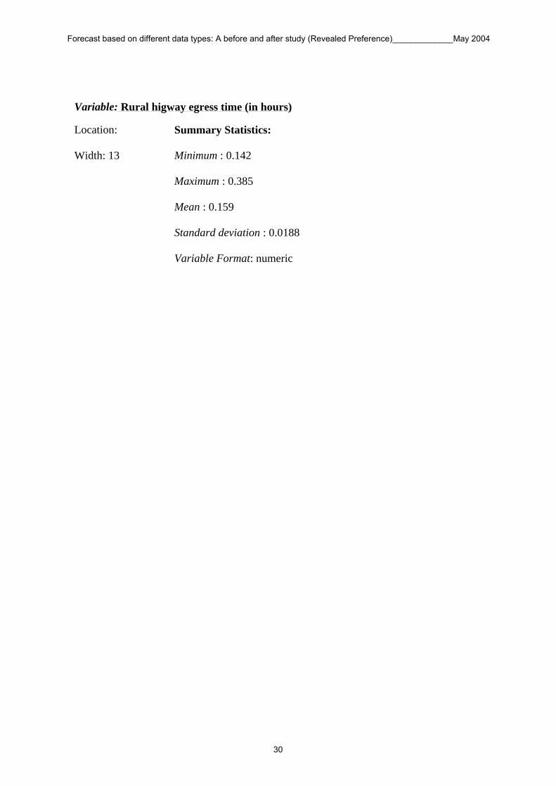
Variable: Rural higway egress time (in hours)
Location:
Width: 13
Summary Statistics:
Minimum : 0.142
Maximum : 0.385
Mean : 0.159
Standard deviation : 0.0188
Variable Format: numeric
Forecast based on different data types: A before and after study (Revealed Preference)_____________May 2004
30
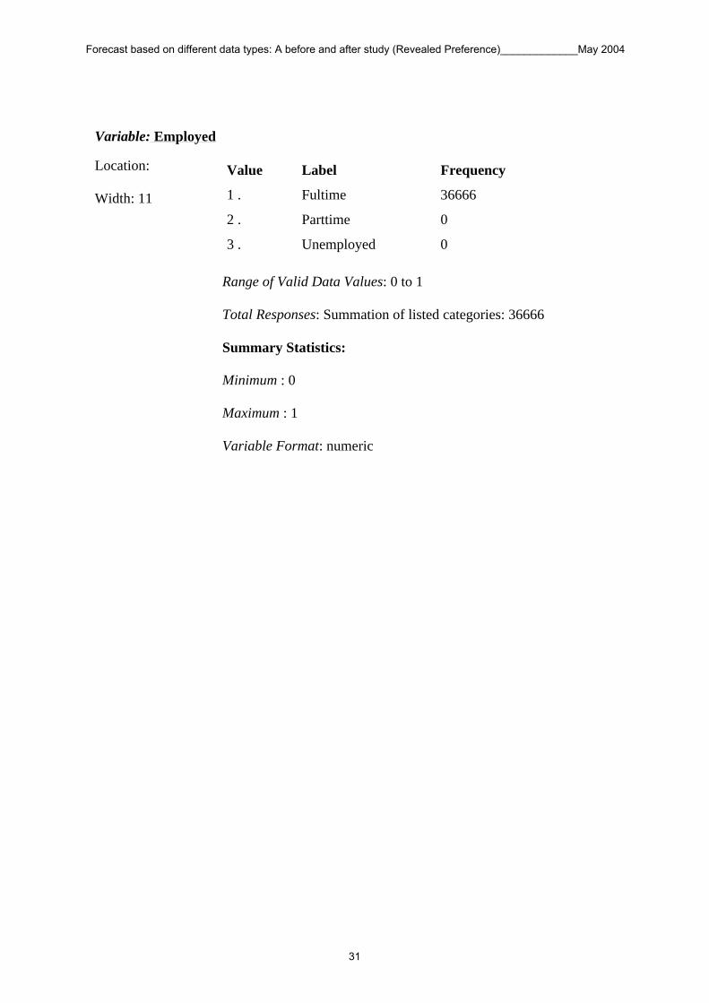
Variable: Employed
Location:
Width: 11
Range of Valid Data Values: 0 to 1
Total Responses: Summation of listed categories: 36666
Summary Statistics:
Minimum : 0
Maximum : 1
Variable Format: numeric
Value Label Frequency
1 . Fultime 36666
2 . Parttime 0
3 . Unemployed 0
Forecast based on different data types: A before and after study (Revealed Preference)_____________May 2004
31

Variable: Occupation
Location:
Width: 11
Range of Valid Data Values: 1 to 3
Total Responses: Summation of listed categories: 46051
Summary Statistics:
Minimum : 1
Maximum : 3
Variable Format: numeric
Value Label Frequency
1 . Selfemployed 3764
2 . Employee 32902
3 . No occupation 9385
Forecast based on different data types: A before and after study (Revealed Preference)_____________May 2004
32

Variable: Cars ownership
Location:
Width: 11
Range of Valid Data Values: 0 to 1
Total Responses: Summation of listed categories: 46051
Summary Statistics:
Minimum : 0
Maximum : 1
Mean : 0.927
Standard deviation : 0.26
Variable Format: numeric
Value Label Frequency
0 . 3350
1 . 42701
Forecast based on different data types: A before and after study (Revealed Preference)_____________May 2004
33
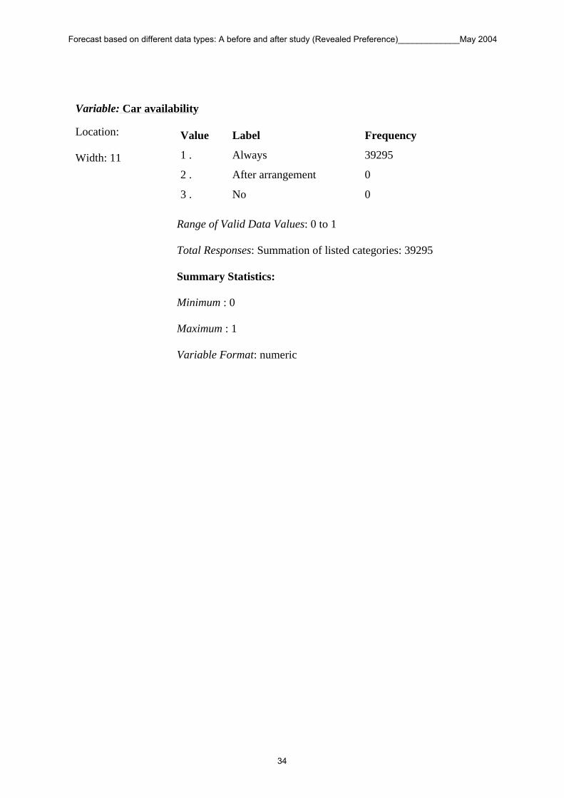
Variable: Car availability
Location:
Width: 11
Range of Valid Data Values: 0 to 1
Total Responses: Summation of listed categories: 39295
Summary Statistics:
Minimum : 0
Maximum : 1
Variable Format: numeric
Value Label Frequency
1 . Always 39295
2 . After arrangement 0
3 . No 0
Forecast based on different data types: A before and after study (Revealed Preference)_____________May 2004
34
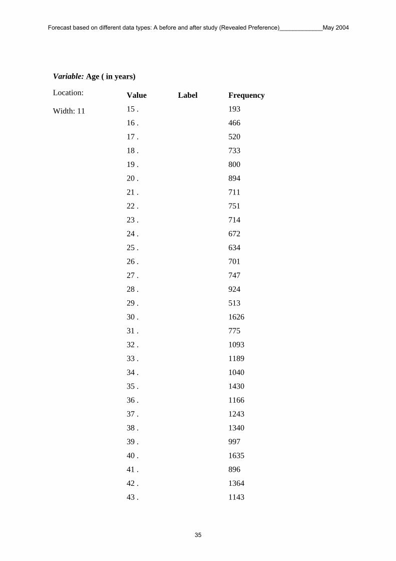
Variable: Age ( in years)
Location:
Width: 11
Value Label Frequency
15 . 193
16 . 466
17 . 520
18 . 733
19 . 800
20 . 894
21 . 711
22 . 751
23 . 714
24 . 672
25 . 634
26 . 701
27 . 747
28 . 924
29 . 513
30 . 1626
31 . 775
32 . 1093
33 . 1189
34 . 1040
35 . 1430
36 . 1166
37 . 1243
38 . 1340
39 . 997
40 . 1635
41 . 896
42 . 1364
43 . 1143
Forecast based on different data types: A before and after study (Revealed Preference)_____________May 2004
35
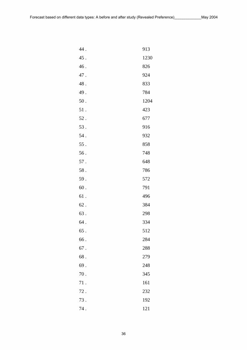
44 . 913
45 . 1230
46 . 826
47 . 924
48 . 833
49 . 784
50 . 1204
51 . 423
52 . 677
53 . 916
54 . 932
55 . 858
56 . 748
57 . 648
58 . 786
59 . 572
60 . 791
61 . 496
62 . 384
63 . 298
64 . 334
65 . 512
66 . 284
67 . 288
68 . 279
69 . 248
70 . 345
71 . 161
72 . 232
73 . 192
74 . 121
Forecast based on different data types: A before and after study (Revealed Preference)_____________May 2004
36
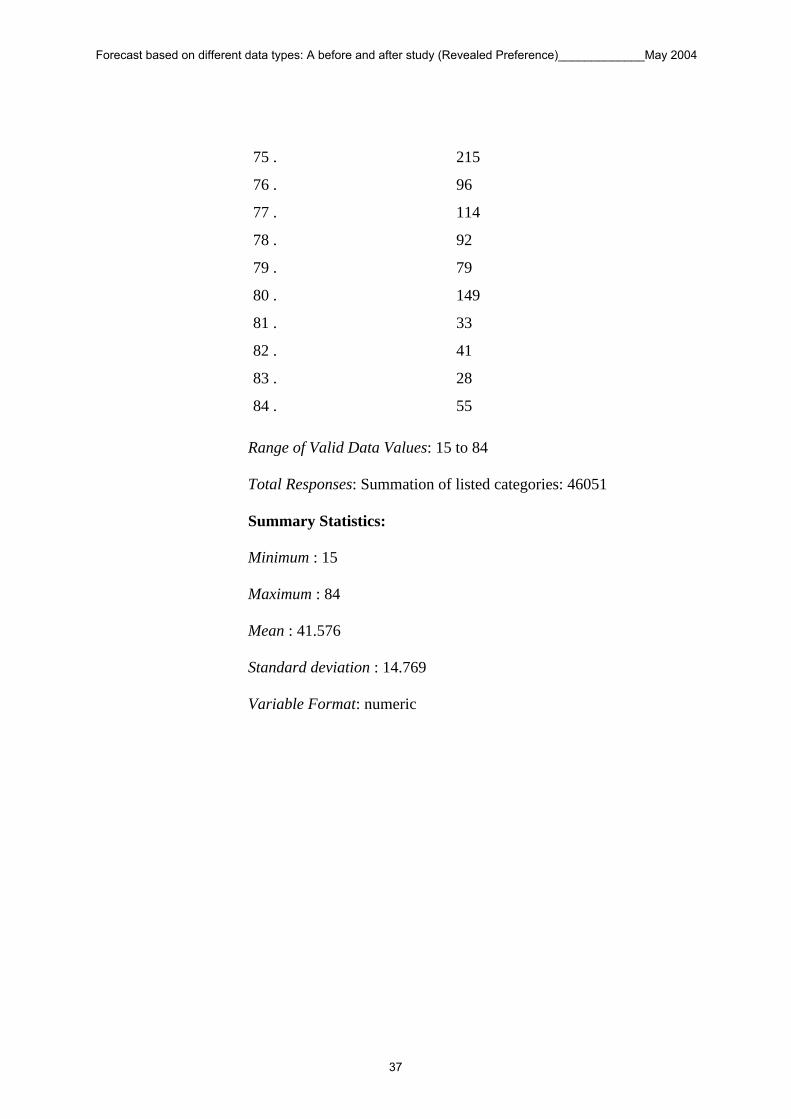
Range of Valid Data Values: 15 to 84
Total Responses: Summation of listed categories: 46051
Summary Statistics:
Minimum : 15
Maximum : 84
Mean : 41.576
Standard deviation : 14.769
Variable Format: numeric
75 . 215
76 . 96
77 . 114
78 . 92
79 . 79
80 . 149
81 . 33
82 . 41
83 . 28
84 . 55
Forecast based on different data types: A before and after study (Revealed Preference)_____________May 2004
37

Variable: Gender
Location:
Width: 11
Range of Valid Data Values: 0 to 1
Total Responses: Summation of listed categories: 46051
Summary Statistics:
Minimum : 0
Maximum : 1
Variable Format: numeric
Value Label Frequency
0 . Female 19290
1 . Male 26761
Forecast based on different data types: A before and after study (Revealed Preference)_____________May 2004
38
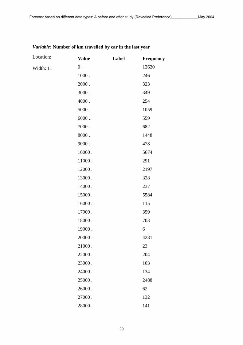
Variable: Number of km travelled by car in the last year
Location:
Width: 11
Value Label Frequency
0 . 12620
1000 . 246
2000 . 323
3000 . 349
4000 . 254
5000 . 1059
6000 . 559
7000 . 682
8000 . 1448
9000 . 478
10000 . 5674
11000 . 291
12000 . 2197
13000 . 328
14000 . 237
15000 . 5584
16000 . 115
17000 . 359
18000 . 703
19000 . 6
20000 . 4281
21000 . 23
22000 . 204
23000 . 103
24000 . 134
25000 . 2488
26000 . 62
27000 . 132
28000 . 141
Forecast based on different data types: A before and after study (Revealed Preference)_____________May 2004
39

Range of Valid Data Values: 0 to 99000
Total Responses: Summation of listed categories: 46051
Summary Statistics:
Minimum : 0
Maximum : 99000
Mean : 13413.237
Standard deviation : 14917.465
Variable Format: numeric
30000 . 2153
32000 . 8
33000 . 12
35000 . 476
38000 . 39
40000 . 754
42000 . 10
45000 . 137
46000 . 14
48000 . 26
50000 . 498
55000 . 14
60000 . 160
65000 . 13
70000 . 56
74000 . 2
75000 . 6
80000 . 80
90000 . 30
99000 . 483
Forecast based on different data types: A before and after study (Revealed Preference)_____________May 2004
40
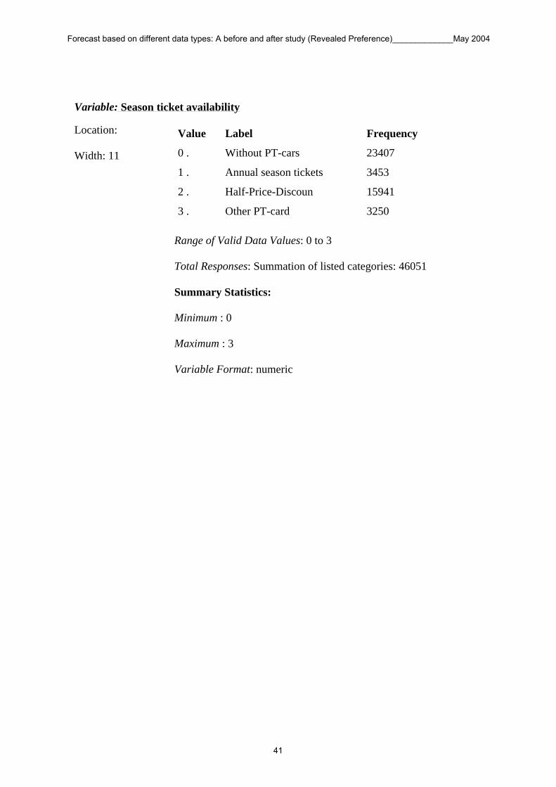
Variable: Season ticket availability
Location:
Width: 11
Range of Valid Data Values: 0 to 3
Total Responses: Summation of listed categories: 46051
Summary Statistics:
Minimum : 0
Maximum : 3
Variable Format: numeric
Value Label Frequency
0 . Without PT-cars 23407
1 . Annual season tickets 3453
2 . Half-Price-Discoun 15941
3 . Other PT-card 3250
Forecast based on different data types: A before and after study (Revealed Preference)_____________May 2004
41

Variable: Trip purpose
Location:
Width: 11
Range of Valid Data Values: 1 to 4
Total Responses: Summation of listed categories: 46051
Summary Statistics:
Minimum : 1
Maximum : 4
Variable Format: numeric
Value Label Frequency
1 . Commuters 22012
2 . Business 1363
3 . Shopping 6854
4 . Leisure/vacation 15822
Forecast based on different data types: A before and after study (Revealed Preference)_____________May 2004
42

Variable: Mode choice to train station
Location:
Width: 4
Total Responses: Summation of listed categories: 46051
Summary Statistics:
Variable Format: character
Value Label Frequency
0 . No 8023
1 . Walk 17314
2 . Urban train/bus 8948
3 . Cars as driver 6754
4 . Cars as passenger 1131
5 . Bicycle 3172
6 . Motorbike, bike 286
7 . Taxi 297
8 . Others 57
9 . Unknown 69
Forecast based on different data types: A before and after study (Revealed Preference)_____________May 2004
43

Variable: Person in household
Location:
Width: 11
Range of Valid Data Values: 1 to 13
Summary Statistics:
Minimum : 1
Maximum : 13
Mean : 2.874
Standard deviation : 1.379
Variable Format: numeric
Forecast based on different data types: A before and after study (Revealed Preference)_____________May 2004
44