0

for Salmon and Watersheds

Sampling Design and Statistical Analysis Methods for the Integrated Biological and Physical Monitoring of Oregon Streams Report Number: OPSW-ODFW-2002-07

0

The Oregon Department of Fish and Wildlife prohibits discrimination in all of its programs and services on the basis of race, color, national origin, age, sex or disability. If you believe that you have been discriminated against as described above in any program, activity, or facility, please contact the ADA Coordinator, P.O. Box 59, Portland, OR 97207, 503-872-5262. This material will be furnished in alternate format for people with disabilities if needed. Please call 541-757-4263 ext. 223 to request.

0

Sampling Design and Statistical Analysis Methods for the

Integrated Biological and Physical Monitoring of

Oregon Streams

Prepared by Don L. Stevens, Jr.

Department of Statistics Oregon State University

Corvallis, Oregon

June 2002

The research described in this article has been funded by the U.S. Environmental Protection Agency. This document has been prepared at the EPA National Health and Environmental Effects Research Laboratory, Western Ecology Division, in Corvallis, Oregon, through Contract 68-C6-0005 to Dynamac International, Inc and Cooperative Agreement CR82-9096-01 to Oregon State University. It has been subjected to Agency review and approved for publication. The conclusions and opinions are solely those of the authors and are not necessarily the views of the Agency. Mention of trade names or commercial products does not constitute endorsement or recommendation for use.

i

TABLE OF CONTENTS

PREFACE .................................................................................................................................... 1

1.0 INTRODUCTION................................................................................................................. 2

2.0 DESIGN CRITERIA............................................................................................................. 2

2.1 Spatial distribution of sample points .............................................................................. 2

2.2 Design flexibility ............................................................................................................... 3

2.3 Provision for trend detection........................................................................................... 3

2.4 Design-based variance estimator..................................................................................... 4

3.0 SAMPLING DESIGN ADULT COHO, JUVENILE COHO, AND HABITAT ASSESSMENT ............................................................................................................................ 4

3.1 Oregon DEQ Sample........................................................................................................ 7

4.0 DATA ANALYSIS AND POPULATION INFERENCE................................................... 8

4.1 Population status estimation............................................................................................ 9

4.2 Trend description ........................................................................................................... 10

REFERENCES.......................................................................................................................... 12

APPENDIX 1: ESTIMATION OF MEANS, TOTALS, AND DISTRIBUTION FUNCTIONS FROM PROBABILITY SURVEY DATA .................................................A.1.1

Statistical Framework ......................................................................................................A.1.1

Estimation of Totals and Means under Variable Probability Sampling Designs.......A.1.1

Variance Estimation.........................................................................................................A.1.2

Confidence Interval Estimation ......................................................................................A.1.5

Subpopulation Estimation ...............................................................................................A.1.6

References ........................................................................................................................ A.1.7

ii

APPENDIX 2: EXAMPLE ANALYSIS APPLIED TO NORTH COAST MONITORING AREA......................................................................................................................................A.2.1

Adjustment using an Imputation Model ........................................................................A.2.2

Adjustment using weight modification...........................................................................A.2.4

Estimates of Totals and Means........................................................................................A.2.5

Subpopulation Analyses...................................................................................................A.2.7

Cumulative Distribution Function (cdf) Estimation .....................................................A.2.9

References .......................................................................................................................A.2.12

APPENDIX 3: 1998 NORTH COAST COHO SPAWNER DATA..................................A.3.1

APPENDIX 4: ANNOTATED SPLUS COMMANDS AND FUNCTION DEFINITIONS USED IN APPENDIX 2 ........................................................................................................A.4.1

Splus commands to impute missing values using spatial interpolation via kriging:..A.4.1

Function listings for spatial imputation .........................................................................A.4.2

Splus Commands for Computing Means, Totals, and CDFs........................................A.4.4

Functions for Computing Means and CDFs ..................................................................A.4.6

1

Preface

This report describes the statistical analytical basis of an integrated monitoring program of salmonids

and their habitats in coastal watersheds of Oregon. This monitoring encompasses sampling

conducted by the Oregon Department of Fish and Wildlife for adult spawners, rearing juveniles and

physical habitat. Additionally, the statistical framework presented in this report is the basis of the

sampling design used by the Oregon Department of Environmental Quality to monitor water quality

and macro invertebrates. This monitoring effort was initiated in 1998 as part of The Oregon Plan for

Salmon and Watersheds and represents an unprecedented effort to comprehensively monitor the

status and trends of coastal salmonids and their habitats. The results of this monitoring will be a key

component in assessing the success of the Oregon Plan in restoring watershed health and natural

salmonid production.

Steve Jacobs Leader, Coastal Salmonid Inventory Project Oregon Department of Fish and Wildlife

2

1.0 Introduction The Oregon Department of Fish and Wildlife (ODFW) has conducted surveys of coho salmon spawning on Oregon coastal streams for over 50 years (Jacobs et al. 2001). The initial surveys were done on purposefully selected streams. The sampling design was switched to a stratified random probability design in 1990 (Urquhart and Kincaid, 1999). The current concern with long-term viability of coastal coho populations sparked a review of that design, with an objective of achieving an integrated sampling approach for spawning salmon, juvenile salmon, and freshwater physical habitat. For each for these populations, there was an interest not only in current status in terms of fish numbers or habitat quality, but also in regional temporal trends. In addition, the Oregon Department of Environmental Quality (DEQ) wanted a much smaller sample from the same stream population to measure water quality. The design discussed in this report addresses all of these objectives. 2.0 Design Criteria Any number of designs might be used for sampling an environmental resource. In many cases, attempting to define an a priori "optimum" design is not feasible because of lack of specific knowledge about the population, or because of competing multiple objectives. Nevertheless, there are general characteristics that a good sampling design for an environmental resource will have, and, in many cases, a design with these characteristics will compare favorably in terms of efficiency to a design optimized for any one of the objectives. Briefly, the characteristics a design should have are (1) sample points more or less evenly distributed over the extent of the population; (2) flexibility to incorporate variable probability and subsampling; (3) provision for trend detection, and (4) a design-based variance estimator. Arguments for these characteristics are given below.

2.1 Spatial distribution of sample points The spatial arrangement of the population is a crucial attribute of the population, and any satisfactory design will result in a sample that reflects that spatial arrangement. Nearby elements can interact with one another, and tend to be influenced by the same set of natural and anthropogenic factors. For example, streams in the same drainage basin are influenced by the same set of physical and meteorological conditions, the same underlying geology, and the same set of landscape disturbances. We want to both recognize and exploit the spatial context of the population as an aid in selecting the sample, and want to ensure that the resulting sample has spatial properties reminiscent of the population. Over repeated sampling, a simple random sample (SRS) , where each point is selected independently and at random from the entire population, is guaranteed to preserve and reflect all attributes of the population. The repeated sampling will faithfully reveal varying spatial density, clusters of elements, or voids. However, any single realization of an SRS may result in substantial distortion of spatial pattern. Our efforts are directed towards structuring the sample so as to ensure that a single realization will have sample spatial pattern that has strong resemblance to the population pattern, i.e., so that clusters and voids are picked up and reflected in the sample, to the resolution of the sample. Of course, the resolution depends on both the sample size and the extent of the population domain. A

3

sample of size 100 from a population spread over 10,000 km2 (a sample spatial intensity of 1 point/100 km2) has no chance of discerning 1 km2-size patches. The property that we would like to have is that the achieved random sample size in any arbitrary subregion of the population domain is close to its expected value. Using SRS as a default standard, we define "close" as having smaller substantially variance than an SRS sample of the same spatial intensity. A design that has this property will permit greater flexibility in doing subpopulation analyses, because most reasonably-sized subpopulations will have reasonably-sized samples. A related advantageous property is that having the sample points well-dispersed over the extent of the resource domain tends to result in a lower-variance estimator. This property will hold for any response variable that shows spatial pattern. Whether the pattern is an irregular mosaic or a smooth gradient, a sample point pattern that is more or less spatially regular will tend to be more efficient (lower variance for the same number of samples) than a completely random sample. (See, for example, Munholland and Borkowski (1996), Breidt (1995), Iachan (1985), Olea (1984), Bellhouse (1977), Dalenius et al. (1961), Matérn (1960), Das (1950), Quenouille (1949), Cochran (1946)).

2.2 Design flexibility Most large-scale environmental monitoring programs have identified subsets of the target population that require special attention in the form of more intensive sampling, that is, more sample points per unit of length or area. The particular interest may stem from a scientific interest (the only place where a certain species occurs); stakeholder interest (a watershed supplying a town's drinking water); an environmental health issue (an area known to have toxic contamination); or a regulatory issue (permits for timber harvest in an area inhabited by an endangered species). Furthermore, those special-interest sub-populations will often not be recognized at the time the sample is originally selected. Whatever the source of interest, the design must be able to accommodate it by allowing variable spatial density of the sample points (variable inclusion probability). The design should also provide a means for the sample to be augmented (or, perhaps, reduced) for selected subpopulations at some time after the initial sample selection. Another very common requirement is that the design be amenable to sub-sampling. In our experience, the most frequent source for this requirement has been that a variety of metrics are needed, some of which are prohibitively time-consuming or expensive. The obvious solution is to collect those metrics only on a subset of the sample, and we want to be able to pick the subsample in a manner that preserves the spatial distribution of the subset.

2.3 Provision for trend detection Environmental monitoring programs often have a dual objective of describing both current status and trend in status. An estimate of trend can be obtained from any temporal sequence of samples of the same population by estimating the population mean from each sample in the sequence, and then estimating the trend in mean value. However, a much richer and potentially more sensitive class of trend descriptions can be obtained from samples that were designed to describe both status and trend. A class of sampling designs referred to as survey designs over time (Kish, 1987) meets the dual focus on current status and trend. Rao and Graham (1964) discuss rotation designs for sampling on

4

repeated occasions. Binder and Hidiroglou (1988) review some of these alternative design and analysis approaches for sampling a population through time. Duncan and Kalton (1987) describe the characteristics of sampling designs through time, especially as they apply to human populations. Skalski (1990) recommends sampling with partial replacement designs for long-term environmental monitoring. Urquhart and Kincaid (1999) compare trend detection power for several designs over time. The essential feature of survey designs over time is an organized schedule of revisiting some units or sites from the sample, dropping others, and adding new ones as time passes. Repeat visits to the same sites allow a measurement of site change. Measurement of site change at several sites can be used to get an estimate of population change that does not include the component of variation arising from visiting different sites, e.g., spatial variation. If a site retains much of its identity from year to year, repeat visits will provide a more precise estimate of change or trend than would be available from visiting different sites each year. Moreover, repeat site measurements can lead to a broader class of trend descriptors. For example, with repeat site measurements, trend can be described by the distribution of site-specific trend, instead of only by the trend in population mean value.

2.4 Design-based variance estimator A strength of probability sampling is that the resulting data can be analyzed with minimal reliance on model assumptions. The sampling design itself provides the prescription for the analysis. Estimates of population parameters are usually obtained with little difficulty; estimates of precision can be more difficult to get, depending on the complexity of the design. We impose an explicit requirement on a sampling design that a viable estimator of sampling variance be available. One way to satisfy this requirement is to provide an explicit expression for the inclusion and pairwise joint inclusion probabilities, so that the Horvitz-Thompson (HT) estimator with its associated variance estimator may be applied (Horvitz and Thompson, 1952). If the HT estimator is not used, or the pairwise probabilities are not available, then some other explicit method for variance estimation must be available. 3.0 Sampling design adult coho, juvenile coho, and habitat assessment The design developed for sampling adult coho spawners, juvenile salmon, and habitat is based on a rotating panel concept, and is predicated on the following:

• There are two primary objectives of the sampling: describe current status and describe population trend.

• There is strong biological evidence for a 3-year life cycle for coho, so we anticipate a resemblance between cohorts corresponding to that 3-year cycle.

• There is spatial pattern in the population. • Sites are not impacted by the measurement protocol. • Population (regional) trend is described in terms of the distribution of trend statistics defined

by repeated observations at individual sites. The ODFW classifies the streams on the Oregon coast into 5 Monitoring Areas (MA). Additionally, there are three non-coastal MA's: the Willamette Valley, the Lower Columbia, and Southwest

5

Washington. Each MA forms a distinct reporting unit, and an approximately equal number of samples were allotted to each MA. A GIS coverage of streams was used as a frame for the population. The coverage was based on USGS 1:100000 topographic maps, modified by ODFW to correspond to the target population of streams for each population. The target populations for the three kinds of sample are nested, with the habitat population being the largest, and the spawner streams being the smallest. The desired sample intensity (number of samples/km of stream) is in the opposite order to population extent, with the spawner sample having the highest sample intensity, and the habitat sample the lowest. These facets were considered in designing the sample for ODFW. Because each MA forms a separate reporting unit, the MAs were treated as strata, with samples selected independently between MAs. The same design was used within each MA. To accommodate the need for repeat visits while continuing to expand the scope of the sample every year, we used a rotating panel design, where sets of panels in the design are visited on different multi-year cycles. The design consists of 40 panels, with one panel defining sites visited every year, 3 panels defining sites visited on a 3-year cycle, 9 panels defining sites visited on a 9-year cycle, and 27 panels defining sites visited on a 27-year cycle. An equal number of sites were allotted to each panel. Within each MA, we wanted a spatially well-balanced sample. The US Environmental Protection Agency�s Environmental Monitoring and Assessment Program (EMAP) (Overton, White, and Stevens, 1991; Larsen, et al., 1991; Larsen, et al., 1994; Stevens, 1994; Herlihy, et al., 2000;) uses a sample design called a Generalized Random Tessellation Stratified design (GRTS) (Stevens, 1997; Stevens & Olsen, 1999; Stevens & Olsen, 2000, Stevens & Olsen, in review, 2002) to achieve a spatially-balanced point distribution that is nonetheless random. The GRTS design captures much of the potential efficiency of a completely regular design for any spatially patterned response. Briefly, the GRTS design achieves a random, nearly-regular sample point pattern via a random function that maps 2-dimensional space, e.g., a square, onto a 1-dimensional line. The function is defined recursively in a manner that preserves some 2-dimensional proximity relationships, in particular, the images of two points that are close together in 2-dimensional space will tend to be close together in the 1-dimensional (linear) space. A systematic sample is selected in the linear space, and the sample points are mapped back into 2-dimensional space via the inverse of the random function. The resulting sample will be nearly regular in 2-dimensional space because of the proximity-preserving property of the random function. An irregular 2-dimensional object, such as an MA, can be sampled by enclosing the object in a square, constructing the random function on the square, and then discarding points outside the object. A linear object in 2-dimensional space, such as a stream network, is sampled by assigning a weight of 0 to all points that are not on the network. Details of the construction of the random function and sample selection are provided in Stevens and Olsen (in review, 2002).

6

The sample points for the panels were selected using the GRTS design applied to the ODFW stream frame. The three types of sample sites (spawners, juvenile, and habitat) were chosen as nested samples. Each panel in itself is a spatially well-distributed sample of the entire population in the year it is visited, because of the selection method. The sample selection process is illustrated with the sample for the Mid-Coast MA. The spawning domain comprises approximately 2121.3 km of streams, with about 2678.7 km and 4087.2 km in the juvenile and habitat domains, respectively. The target sample sizes were 164 spawning sites, 56 juvenile sites, and 52 habitat sites per year, so the highest sampling intensity was the spawner sample, with 164/2121.2 = .0773 samples per kilometer of stream (1 sample per 12.9 km of stream). These target sample sizes are used to establish sampling intensities on the frame. To allow for non-target sites, these target sample numbers are somewhat higher than the number of sites for which data will actually be collected. In every year, 4 panels (the panel that is visited every year, plus a 3-year, a 9-year, and a 27-year panel) are visited, with each panel having the same expected number of samples. Thus, each panel should have an expected number of 164/4 = 41 spawning sites. Since there are 40 panels altogether, a total of (40)(41) = 1640 spawning sites are needed, that is, we need 10 times as many sites in the sample as we will visit in any one year. Dividing by total length of stream in the spawning frame yields the sample intensity of 1640/2121.3 = 0.773 samples/km for entire 40 panel sample. (Since only 4 panels are visited in any year, the sample intensity for the annual sample is 0.773/10 = 0.0773 samples/km) The first step in the selection was to map the most extensive frame (the habitat frame) to a line using the random recursive function defined in the GRTS design. The total length of the line was proportional to the total length of the habitat frame, i.e., 4087.2 km. A systematic sample was selected along this line, using a sampling interval proportional to the base sampling intensity of 0.773 samples/km. This resulted in approximately (4087.2)(0.773) = 3160 sample points. These 3160 sample points were divided into 40 panels by splitting them into groups of 40 sequential points, that is, points 1 through 40 into group 1, points 41 through 80 into group 2, and so on. This resulted in 79 groups of 40 points each. The 40 points in a group were randomly assigned to the 40 panels, one to a panel. Because of the proximity-preserving property of the recursive random function, the points within each group of 40 are images from a more or less contiguous portion of the frame. Thus, each panel has a point from that more or less contiguous portion of the frame, and each panel should have about 3160/40 = 79 points that are well-distributed over the entire 4087.2 km in the habitat domain. Because the spawner domain has only 2121.3 km of stream, we expect about 79(2121.3/4087.2) = (79)(0.519) = 41 points in each panel to fall into the spawner domain. The 79 points within each panel have an order inherited from the spatial proximity preserving order of the GRTS design. Any systematic subsample using this order will result in a spatially-well-distributed sample. The juvenile sample was selected as a systematic subsample using the GRTS order. The target sample size is 52 juvenile samples per year, split between 4 panels for 13 samples

7

per panel per year. In each panel of 79 points, we expect 79(2678.7)/4087.2 = 52 points to fall into the juvenile domain. If we assign each of the 79 points a unit length, and take a systematic subsample using a sampling interval of 13(4087.2)/(79(2678.7)) = 0.2511, we expect to get 19.84 samples, of which 19.84(2678.7/4087.2) = 13 are expected to fall in the juvenile domain. Finally, the habitat sample was selected by reducing the expected 19.84 samples to an expected size of 14, again using a systematic sample along the inherited order. The three types of samples were selected as nested subsamples. However, the actual domains do not coincide, so there will be sites where only a habitat sample is taken, or only habitat and juvenile samples are taken. The different kinds of sample will coincide whenever possible, i.e., if a habitat sample is indicated on a stream where coho spawn, a juvenile and spawner sample will also be collected there. In any single year, 4 out of the 40 panels are sampled, so that the annual sample intensity is one-tenth of the overall sample intensity. Thus, for the spawner sample, the annual sample intensity is 0.773/10 = 0.0773 samples/km. This number is the inclusion density (π) used in the analysis. Equivalently, the weight is the reciprocal of the inclusion density, which gives 1/0.0777 = 12.94 km/sample, so that each spawner sample represents 12.94 km of stream.

3.1 Oregon DEQ Sample The sample selected for DEQ is a good illustration of the flexibility that is achieved with the EMAP�s spatially restricted design. The multi-panel ODFW sample design was developed in 1998. In 1998, the DEQ required an equiprobable sample of 50 sites per year from the composite of physical habitat frames of all 8 MA's. Furthermore, the DEQ sample was to be on a 6-year cycle of repeat visits instead of the 3-year base for the ODFW sample. Insofar as possible, the DEQ sites sampled in a year should coincide with the ODFW physical habitat sites sampled in that year. In 1999, the DEQ wanted to extend the frame of the ODFW sample in the Willamette Valley. Furthermore, instead of an equi-probable sample, they wanted to ensure samples on 2nd and 3rd order streams, but otherwise to take a proportional subsample of the ODFW sites in the coastal MA�s. In 2000, the DEQ was concerned that the sample sizes in the Willamette Valley were too small, and wanted to sample sites in 2000 that were scheduled for visits in later years. All of these objectives were accommodated. The 1998 requirements were met by utilizing the GRTS ordering of the stream network, and the inherited order of the ODFW habitat sample. We in effect created a sample line consisting of the physical habitat samples from all of the MAs. The samples from a single MA occupied contiguous positions on the line, in their inherited random order. Differences in inclusion density between MAs were accounted for by adjusting the length assigned to each MA to get constant proportionality between frame and population stream length. Since DEQ wanted a different re-visit schedule, we had to define another panel structure consisting of sites visited annually, sites visited on a 6-year rotation, and sites visited o a 36-year rotation. The ODFW panel structure was translated into the DEQ structure so as to maximize temporal coherence of the two samples.

8

The 1999 DEQ coastal subsample was selected by ordering the 2nd and 3rd stream order sites within MA using their GRTS random order, randomly ordering the MA's, and then systematically assigning every other site to a base sample. The sites should be roughly evenly spread over panel and MA, with almost 2 sites per panel per MA. Since 4 panels are visited each year, this should give about 4x2x5 = 40 visits per year on 2nd and 3rd order streams. The 1st order sites were selected by using the GRTS random order within MA, and randomly ordering across MA. Every 9th site was assigned systematically to the base sample. This resulted in approximately 200 sites in the base sample, or approximately 5 sites per panel. Since 4 panels are visited each year, this should give about 20 visits to 1st order streams per year in the base sample. The 1999 DEQ Willamette Valley sample was selected by adding a USGS GIS coverage to the frame used to select the ODFW sample. The procedure used was to pass the USGS frame through exactly the same sample selection procedure as used for the ODFW sample, using the same GRTS random function, the same stream order weights, and the same systematic selection procedure. This resulted in approximately 1700 sites, approximately evenly distributed among panels and approximately evenly distributed over stream order. The sites for each panel were arranged in their inherited GRTS order, with the USGS sites following the ODFW sites. A 1/13 subsample was selected using a systematic selection with a random start, independently for each panel The need to add more points in 2000 was accommodated by �collapsing� the temporal structure of the panels, so that each 9-year panel became three 3-year panels, and each 27-year panel became three 9-year panels. This action nearly doubled the sites available for sampling in 2000. 4.0 Data analysis and population inference The population status description will be accomplished using the usual EMAP descriptive analyses (Diaz-Ramos, et al., 1996). The general approach is sketched briefly here, with details in Appendices 1 through 3. Appendix 1 has the details of the statistical methodology for population inference. Appendix 2 contains details of estimates for the 1998 North Coast data set, which is provided in Appendix 3. The objective of the sampling design is to determine some attributes of a network of streams. Those attributes are quantities such as the total number of salmon spawners in the network, the average number of spawners per kilometer of stream, etc. We select the sample from the perspective that we are sampling a one-dimensional continuum (the lines comprising the stream network), and measuring the value of some function defined on that continuum. For example, the function might be the spawner density expressed as number of spawners per kilometer of stream. The integral of that function over the extent of the network will then yield the total number of spawners in the network. The spawner density function only exists in the abstract until we give it substance by defining how we are going to measure it. A common approach in EMAP for similar kinds of functions is to define a density function at a point s in the network as the total over a fixed stream length l centered on s, divided by l. One can think of the stream segment as a window containing s, so that we calculate the density at s by adding up everything within the window and dividing by the extent of the window. As

9

s moves over the extent of the network, the window moves along with it, and we end up defining a more or less continuous function representing the local average density. The only potential difficulties occur near the endpoints of segments in the network. If we are careful with our definitions at those points, then we obtain a density function with the property that its integral over the network is equal to the total of the attribute over the network (See Stevens and Urquhart, 2000, for details). The ODFW protocol is similar, but the window is not a fixed length of stream centered on the point. Instead, the stream network is broken into segments defined by physical characteristics of the stream, with the constraint that segments should all have about the same length. The "window" for a point s is taken to be the segment containing s. Every point on a segment has the same window, and thus every point on the segment is assigned the same value of the density function. It follows that he density function in this case is a step function, that is, it changes values only at the endpoints of segments, where it jumps abruptly from the average over one segment to the average over the next. Even though this function is not continuous, it nevertheless has the property that its integral over the extent of the network yields the total number in the network. The sampling scheme picks out points on the network at which values of the network attributes, e.g., the density function, are to be observed. The analysis is aimed at estimating totals, means, and distribution functions of those attributes for the network or subsets thereof. It is important to note that the sampling design and analysis is guaranteed to produce unbiased estimators of the properties of the functions that have been accumulated over the window. Those properties can be impacted by the choice of window. For example, larger windows (that is, longer stream segments) will, other things being equal, lead to a less variable response function.

4.1 Population status estimation The recommended estimator is the Horvitz-Thompson or π-estimator. It is described fully in Appendix 1. Briefly, the estimator weights the observation collected at si by the reciprocal of the inclusion density function π(si). Annual status estimates are obtained from all sites visited in that year. The design selects points on streams. Suppose point si falls on a stream segment with length li. The observation collected represents an aggregate over the entire length of the segment. Thus, if the observation is spawner count, then the entire segment is examined for spawners, and all spawners in the segment are counted. Let yi be the aggregated observation. Then an estimator of the total number of spawners

over the entire stream network is �n

iT i

ii

yY = ( )/ (s )l

π� where n is the number of samples. Moreover,

within a MA, π(s) is constant, so, letting 1c = (s)π

, the estimator becomes �n

iT

ii

yY = c ( )l� . More

details on estimation of totals, averages, and confidence limits are in Appendix 1.

From the design perspective, we can view the design for a MA as a �multi-phase� design, consisting of a number of design phases nested within one another. From this perspective, the collection of all

10

sites visited over 27 years is a single sample. Each point in the sample (the first phase) is visited at least once in the 27-year duration of the design. A subset (the second phase sample) of the first phase is visited at least three times over 27 years. The second phase consists of those sites in the 9-year, the 3-year, and the annual panels. The third phase of the design is those sites visited at least 9 times in 27 years, and consists of the 3-year and annual panels. Finally, the fourth phase consists of the annual panels, i.e., those that are visited 27 times during the 27 years. Thus, each successive phase is a subset of the preceding phase. The advantage of this viewpoint is that a variety of analysis techniques are available for multi-phase designs (see, for example, Sarndal, Swensson, and Wretman, 1992). Within the multi-phase paradigm, for example, we have (1) composite estimators of current status, which use prior years data to improve current years estimators, (2) multi-phase regression, which uses ancillary information that need not be available on all phases. This last technique could be a very powerful way of describing regional trend. Composite estimators make use of the revisit pattern to use data from previous years to improve annual status estimates. The basic concept is that we have a model that predicts the response for location s at time t+1 based on the response at time t. The model predictions from all sites visited at time t are used to estimate the mean at time t+1. Residuals at the re-visit sites are used to estimate the difference between the model-based mean and the true mean, and the estimated difference is used to correct the model-based mean. This correction term makes the adjusted model-based mean design-unbiased. We get a second design-unbiased estimate from the sites visited only at time t+1. Any convex combination of the two estimates of the mean is also design-unbiased. If the model prediction is reasonably accurate, the composite estimator will have lower variance than the estimator based solely on the sites observed at time t+1. A simple model to predict the value at t+1 for a site observed at t is simply to use the observed value. In fact, the usual application of composite estimation relies on the temporal correlation between revisits. We could extend that to draw on the space-time covariance model, or more generally, on any model that predicts a response at time t and location s based on ancillary variable and responses from previously observed times and locations. This can be done so that the resulting estimates remain design-based/model-assisted, so that even if we don�t get the model exactly right, our estimates are still design-unbiased. The utility of these estimators is that they �borrow strength� from data that are nearby in space or time. The result is that we get more precise estimators, that is, estimators with smaller variance, provided our model is reasonably accurate.

4.2 Trend description The sample design will allow description of population trend in the familiar form of a pattern of change in (population) mean value, and will also allow estimation of the distribution of trend statistics at individual sites. Specifically, we propose that multi-phase regression analyses be used to estimate the distribution of trend statistics. The analysis is sketched out below. A design-based approach to describing regional trend is to characterize the population of site-specific

11

trends. Suppose we observe a site once a year for 27 years. We could describe the trend at that site by a statistic such as the slope coefficient from a linear regression of the response on year number. We can regard the slope itself as a response variable, and think about having it available at every point in a MA. The population of slope coefficients characterizes trend for the MA, and we can summarize that population in a variety of ways, just as we would summarize any other population response. For example, we can calculate statistics such as the mean and variance; the population distribution function; or the percentage of the population that has a positive trend. Of course, our sample does not give us information at every point in the MA, but we do have one panel of sites that were visited every year. From that one panel, we can estimate population parameters. We can make use of the multi-phase aspect of the sample to utilize data from the other panels. Besides the slope statistic based on all 27 years of data, we could also calculate a �3-year� slope based on observations 3 years apart, e.g., on observation from years 1,4,7,10,13,16,19,22, and 25. We would not expect to get the same number as for the 1-year interval data (the 1-year slope), but over the entire population, we would expect the 3-year slope to be strongly correlated with the 1-year slope. From our sample, we can calculate the 1-year slope only for the sites that are observed every year (Phase 4 data), but we can calculate the 3-year slope for both annual and 3-year sites (Phase 3 data). The idea behind multi-phase regression is that we use the 3-year slope to predict the 1-year slope for the 3-year sites. Since we can calculate both the 1-year and the 3-year slopes for the annual sites, we can use the annual site data (Phase 4) to estimate regression coefficients for predicting 1-year slopes from 3-year slopes. We have 3-year slopes available for the Phase 3 sites, so we can use the regression equation to predict 1-year slopes for all of the Phase 3 sites. The predictions are then used together with the observed 1-year slopes from Phase 4 to get more precise estimates for the population of 1-year slopes. We can also carry the analysis a step further, by estimating 9-year slopes, and predicting 1-year slopes from the observed 9-year slopes. Eventually, if we go back to the 27-year sites beginning in year 28, we could also incorporate 27-year slopes. Essentially, the technique allows us to fill in trend data for sites that were not observed every year. If the correlation between the 1-year and 3-year slopes is high, then we can expect a substantial increase in precision, since we will have effectively quadrupled our sample size. Multi-phase regression works with any estimator of slope, so we are not limited to using linear least-squares regression. For example, there are several non-parametric alternatives, such as the Sen slope (Sen, 1968), or various robust/resistant estimators, such as lowness (Cleveland, 1979). One could even use a model-based estimator of slope, e.g., one based on a space-time model. The key to applying multi-phase regression to describe trend is that we regard the trend estimator based on the complete record of annual observations as the site response. Observations at sites not observed every year are used as ancillary variables to predict the response at those sites. Multi-phase regression provides the analytic framework in which to develop the population-level estimates of trend.

12

References Bellhouse, D.R. (1977). �Some optimal designs for sampling in two dimensions'. Biometrika 64,

605�611. Binder, D.A., and M.A. Hidiroglou. (1988). Sampling in Time. In: Handbook of Statistics Vol. 6,

"Sampling." P.R. Krishnaiah and C.R. Rao, eds., pp. 187-211. Elsevier Science Publishers B.V. Amsterdam, The Netherlands.

Breidt, F.J. (1995). �Markov chain designs for one-per-stratum sampling�. Survey Methodology 21:1,

63-70. Cochran, W.G. (1946). �Relative accuracy of systematic and stratified random samples for a certain

class of populations. Annals of Mathematical Statistics 17, 164�177. Cordy, C. (1993). �An extension of the Horvitz-Thompson theorem to point sampling from a

continuous universe'. Probability and Statistics Letters 18, 353�362. Cotter, J., and J. Nealon. 1987. Area Frame Design for Agricultural Surveys. Area Frame Section,

Research and Applications Division, National Agricultural Statistics Service, U.S. Department of Agriculture.

Cleveland, W. S. (1979). Robust locally weighted regression and smoothing scatterplots. Journal of

the American Statistical Association 74, 829-836 Dalenius, T., J. Hájek, and S. Zubrzycki. (1961). �On plane sampling and related geometrical

problems'. Proceedings of the 4th Berkeley Symposium on Probability and Mathematical Statistics 1, 125�150.

Diaz-Ramos, S., D.L. Stevens, Jr, and A.R. Olsen. (1996). EMAP Statistical Methods Manual.

Environmental Monitoring and Assessment Program, National Health and Environmental Effects Research Laboratory, Office of Research and Development, Corvallis, OR.

Duncan, G.J., and G. Kalton. (1987). �Issues of design and analysis of surveys across time'.

International Statistical Review 55:97-117. Gibson, L. and D. Lucas. (1982). �Spatial data processing using balanced ternary'. Proceedings of the

IEEE Computer Society Conference on Pattern Recognition and Image Processing. Silver Springs, MD: IEEE Computer Society Press.

Hájek, J. (1971). �Comment on a paper by D. Basu. In: Godambe, V. P., and Sprott, D. A. (eds.)

Foundations of Statistical Inference. Toronto: Holt, Rinehart, and Winston, p. 236.

13

Horvitz, D.G. and D.J. Thompson. (1952). �A generalization of sampling without replacement from a finite universe'. Journal of the American Statistical Association 47, 663�685.

Jacobs S., J. Firman, and G. Susac (2001). Status of Oregon coastal stocks of anadromous

salmonids, 1999-2000; Monitoring Program Report Number OPSW-ODFW-2001-3, Oregon Department of Fish and Wildlife, Portland, Oregon.

Kish, L. (1987). Statistical Designs for Research. John Wiley & Sons. New York. Mark, D.M. (1990). �Neighbor-based properties of some orderings of two-dimensional space'.

Geographical Analysis 2:145-157. Madow, W.G. (1949) �On the theory of systematic sampling, II' Annals of Mathematical Statistics

20: 333-354. Munholland, P.L., and J.J. Borkowski. (1996). �Simple Latin square sampling +1: A spatial design

using quadrats�. Biometrics 52: 125-136. Matérn, B. (1960). Spatial Variation. Stockholm, Sweden: Meddelanden från Statens

Skogsforskningsinstitut. Rao, J.N.K., and J.E. Graham. (1964). �Rotation designs for sampling on repeated occasions�. JASA

59:492-509. Saalfeld, A. (1992). �Construction of spatially articulated list frames for household surveys�. In:

Proceedings of Statistics Canada Symposium 91. Spatial Issues in Statistics. Ottawa, Ontario, Canada: Statistics Canada, 41-53.

Särndal, C., B. Swensson, and J. Wretman. (1992). Model Assisted Survey Sampling. Springer-

Verlag. New York. Sen, P.K. 1968. �Estimates of regression coefficient based on Kendall's tau�. Journal of the American

Statistical Association 63:1379-1389. Sen, A.R. (1953). �On the estimate of the variance in sampling with varying probabilities�. Journal

of the Indian Society of Agricultural Statistics 7, 119�127. Simmons, G.F. (1963) Introduction to topology and modern analysis. McGraw-Hill. New York. Skalski, J.R. (1990). �A design for long-term status and trends monitoring�. Journal of

Environmental Management 30:139-144.

14

Stevens, D. L., Jr. (1994). �Implementation of a national environmental monitoring program�. Journal of Environmental Management 42: 1�29.

Stevens, D.L., Jr. (1997). �Variable density grid-based sampling designs for continuous spatial

populations'. Environmetrics 8: 167-195. Stevens, D. L., Jr., and T. M. Kincaid. (1997). �Variance estimation for subpopulation parameters

from samples of spatial environmental populations'. Proceedings of the American Statistical Association Section on Statistics and the Environment, American Statistical Association, Alexandria, VA.

Stevens, Jr., D. L. and A. R. Olsen. (1999). �Spatially Restricted Surveys Over Time for Aquatic

Resources'. Journal of Agricultural, Biological, and Environmental Statistics 4:415-428. Stevens, Jr. D.L., and N.S. Urquhart. (2000). Response Designs and Support Regions in Sampling

Continuous Domains. Environmetrics 11:13-41 Stevens, Jr., D.L., and A. R. Olsen. (In review, 2002). �Spatially-Balanced Sampling of Natural

Resources in the Presence of Frame Imperfections� Stevens, Jr., D.L., and A. R. Olsen. (In review, 2002). �Variance Estimation for Spatially

Balanced Samples of Environmental Resources� Thompson, S.K. (1992). Sampling. New York: John Wiley & Sons. Urquhart, N.S., W.S. Overton, and D.S. Birkes. (1991). Comparing Sampling Designs for

Monitoring Ecological Status and Trends: Impact of Temporal Patterns. Technical Report 149. Department of Statistics, Oregon State University, Corvallis, Oregon.

Urquhart, N.S., and T.M. Kincaid. (1999). �Trend detection in repeated surveys of ecological

responses�. Journal of Agricultural, Biological, and Environmental Statistics 4: 404:414. White, D., A.J. Kimmerling and W.S. Overton. (1992). �Cartographic and geometric components of

a global sampling design for environmental monitoring'. Cartography and Geographic Information Systems 19, 5�22.

Wolter, K.M., and R.M. Harter (1990). �Sample maintenance based on Peano keys'. In: Proceedings

of the 1989 International Symposium: Analysis of Data in Time. Ottawa, Ontario, Canada: Statistics Canada, 21-31.

Yates, F. and P.M. Grundy. (1953). �Selection without replacement from within strata with

probability proportional to size'. Journal of the Royal Statistical Society B15, 253�261.

A.1.1

Appendix 1: Estimation of Means, Totals, and Distribution Functions from Probability Survey Data

Statistical Framework We base the development here on the case of a response z(s) defined on a region R that is a subset of a universe U, which we assume is a 2- or 3-dimensional continuum. Our objective is to estimate some properties of the response on R. In particular, we want estimates of the total ZT, the mean value

z(R )µ and the distribution function (zF x) of the response over R. We define these by TR

Z = z(s)ds� ,

Tz

Z(R ) = | R |

µ , and ( )z { s | z(s) x }R

1F (x) = I s ds| R | ≤� where |R| denotes the size (length, area, volume) of R

and IA(x) is the indicator function for A, that is, it indicates whether the point x is in the set A.

Formally, IA(x) is defined as otherwiseA

1, x AI ( x) =

0, ∈�

��

. Because ( ){ s | z(s) x }R

I s ds≤� is the size of the set

for which the response meets the condition z(s) ≤ x, the distribution function (zF x) measures the fraction of R for which the condition is met. A probability sample from R is a set S = {s1, s2,�, sn } of n random points in U. The usual requirement for a probability sample that is the probability distribution of the sample be known. We are basing the development here on the assumption that we are sampling a spatial continuum, so we assume that we know (or can calculate) the spatial sampling intensity function (also called the inclusion probability density function) π(s). The function π(s) describes the average density of our sampling points, and has units of number of points per unit length or area. Thus, for a stream sample, π(s) would have units of number of points per kilometer of stream.

Estimation of Totals and Means under Variable Probability Sampling Designs Horvitz and Thompson (HT)(1952) provided an estimator of the population total for variable-probability, without-replacement, finite-population sampling designs, along with an expression for the variance of the estimated total and a related variance estimator. Cordy (1993) showed that a version of the HT theorem holds when sampling from a continuum U. The continuous version of the HT theorem provides estimators of the total (integral) of z over R An estimate of the mean is obtained by dividing the estimated total by |R|, the size of R. An alternative estimator of the mean, called a ratio estimator, uses the estimated size of R as the divisor. As in the finite population case, the ratio estimator of the mean (also known as the Hájek estimator (Hájek, 1971; Thompson, 1992)) tends to be nearly unbiased and less variable because of positive correlation between the numerator and denominator. It is also well-suited to subpopulation estimation, as the size of subpopulation domain need not be known.

Let s1, s2, ..., sn be a sample selected from a universe U according to a design with inclusion function π(s). For an arbitrary region R ⊂ U, an unbiased estimator of ( ) T

R

z s ds Z=� is

A.1.2

A.1.1 . ) s(

) sz( ) s(I = Zi

iiRn

1 = iT π

��

An (approximately) unbiased ratio estimator of mean value of z, i.e., of | R | / z(s)ds = ) (RR

z �µ is

A.1.2 ��� ,�

nR i i T

zii = 1

Z( ) z( )s sI = / | R | = ( ) | R |s

µπ�

where )s()s(I = | R|

i

iRn

1 = i π�� .

The inclusion density specifies the number of points per unit of population, e.g., number of points per mile of stream. Its reciprocal, then, specifies the units of population per point, e.g., the miles of stream per point. Thus, the reciprocal of the inclusion density of a point specifies the amount or weight of the population represented by that point. We can use this observation to re-express A.1.1

and A.1.2 as weighted sums by letting 1( )( )i

i

w ssπ

= :

A.1.3 � ( )n

R i iiTi = 1

= ( ) w s z( )s sIZ �

and

A.1.4 ( ) ( ) ( ) �

� �( ) ( )

n

R i i ii = 1 T

z n

R i ii = 1

I s w s z sZ = = .| R | I s w s

µ�

�

The spatially restricted design used to select the ODFW sample has inclusion functions that are constant within Monitoring Areas (MAs). If the region R is an MA (or is contained within a single MA), then the ratio estimator of the mean value is identical to the usual estimator, i.e., it reduces to the sum of the observations divided by the number of observations. However, if R includes points from several MAs, that is, if all of the points do not have the same inclusion probability, then the general formula given above must be used.

Variance Estimation The spatial balance inherent in the GRTS design will give a more precise (less variable) estimate of the mean than would a simple random sample of the same size, if the response has some spatial pattern. While the spatial balance will generally lead to more precision, it also complicates estimation of that precision. Intuitively, this happens because the locations of the sample points are not independent of one another, and that dependence must be taken into account in estimating variance. Horvitz and Thompson (1952) provided a general formula for the variance of the estimated mean from a probability sample that accounts for the pairwise dependence of the points, along with an unbiased estimator of the variance. Alternative expressions for the variance and its estimator have been provided by Yates and Grundy (1953) and Sen (1953). These estimators do not work well for a

A.1.3

GRTS design because, although theoretically unbiased, they tend to be very unstable, sometimes even taking on negative values. A simplified and stable estimator for the variance of the mean can be obtained by treating the sample as if it arose from independent random sampling (IRS), where the n points are selected independently from an arbitrary density f(s) over U. In the approximation, n is the number of points in the sample from the universe, not nR, the number of points in the sample that fall in R. If we use this approximation as a variance estimator for a subpopulation, we need to recognize the fact that nR is a random variable. The most straightforward way to do that is to view the variance estimator as conditional on the achieved sample size. This changes the interpretation slightly, but it makes the computation much simpler. The difference in interpretation is that sampling variance describes the variation in the estimator over repeated selections of the sample. The sampling variance conditional on the achieved sample size describes variation in the estimator over the restricted set of repeated selections of the sample that result in the same achieved sample size for R. If we adopt this approach, and set the "n" equal to the achieved sample size in the subpopulation we are dealing with, then the IRS variance estimator for the total is

A.1.5 ,(wz)nV = )(z/nV = )Z(V SRSSRSTIRS π�� where VSRS(z/π) is the usual estimator of the population variance for an SRS design applied to z(si)/π(si) = w(si)z(si). VSRS(Χ) is the default variance estimator available in most statistical software packages. Furthermore, if the inclusion density is constant on the subpopulation (as it is within an MA), then the result further simplifies to

A.1.6 (z)Vnw = (z)/nV = )Z(V SRS

22SRSTIRS π��

as an estimator of the variance of the estimated total ZT� . It follows that the corresponding variance estimator for µ� z is the usual SRS estimator for the variance of the mean: A.1.7 . (z)/nV = )(V SRSzIRS µ��

The IRS estimator does not account for the spatially constrained nature of the design. If the response has some spatial pattern, at least to the extent that two points close together tend to be more similar than two points far apart, then the spatially balanced design will lead to more precise estimates than independent random sampling. Thus, the IRS estimator will be conservative, i.e., it will tend to overstate the variance.

A.1.4

An approximately unbiased estimator of variance can be based on the observation that the spatially constrained nature of the design ensures that any arbitrary subset of the domain will have an achieved sample size nearly equal to its expected sample size (Stevens and Olsen, in review, 2002). If we were to split the population domain up into small neighborhoods, each with an expected sample size of, say, 4 to 5 points, then every replication of the design would place some points in each of the small neighborhoods. Because we can break down the estimated total into the sum of the estimated totals in each of the small neighborhoods, we can break down the variance of the total into the sum of variances of the neighborhood totals. This is the concept behind the neighborhood variance estimator �NBV . The formula for �

NBV is

A.1.8 { }( )� �( )

i j i ik

2

j kij ikTNB

R D( ) s D( )j ks s s s

z(s ) z s( ) = w - wV Z (s ) sπ π∈ ∈ ∈� � �

In this formula, D(si) is a neighborhood around the sample point si, and the wij are weights that depend on the design. The neighborhoods are defined so that each neighborhood contains at least 4 sample points, and satisfies )sD( s )sD( s jiij ∈⇔∈ . The neighborhoods D(si) are developed by initially including the point itself plus the next 3 nearest neighbors for each point, and then adding to D(si) any points sj such that )sD( s ji ∈ . This ensures the condition that )sD( s )sD( s jiij ∈⇔∈ . The weights wij are selected using the following criteria:

1. The weight wij should be inversely proportional to π(sj) and decrease as the distance between si and sj increases.

2. 1 = w = w j i

ij i

j�� , so that the neighborhood totals are averages over the neighborhoods,

and the sum of the neighborhood totals is equal to the estimated overall total. The weights are developed by first assigning a value that decreases as the rank of the distance between sj and si among the points in D(si) increases and is inversely proportional to π(sj). The formula for the this first step is

)s())s(D(count/1) - )s(rank

j

ij

π( - 1

= w*j i

For example, if D(s1) contained 5 points, the points would be ranked 1 through 5 in order of their distance from s1. Of course, s1 receives rank 1, since it is the closest point to itself. The other 4 points would be ranked in terms of increasing distance from s1. If all of the points have the same inclusion

density, say , ) s( j ππ ≡ then the point with rank 4 would get weight ππ

2/5 = 1)/5) - (4 - (1 . The

A.1.5

weights are normalized to satisfy the constraint on the column totals by setting w

w = w *k i

)sD( s

*j i

j i

ik

�∈

~ .

There is no unique way to satisfy both constraints in criterion (2), so we select the set of weights wij that minimize ) w - w( 2

j ij ij i,

~� while satisfying criteria (2). The constrained minimization problem is

solved using Lagrange multipliers. The unconstrained minimization problem is then

1) - w( 1) - w( + )w - w( w

kj k

ll

j ii

kk

2j ij i

j ,ilkij��+��� γλγλ

~,,

min

The wij are easily eliminated from the set of linear equations obtained by setting derivatives equal to 0. The resulting set of equations in λk and γl is singular, and the Moore-Penrose generalized inverse (Rao and Mitra, 1971) is used to obtain a unique solution for λ�k and γ�l . The minimizing set of weights is

2 +

+ w = w ji*j ij i

γλ ��.

Confidence Interval Estimation A strictly correct confidence interval for an estimator would be based on the sampling distribution of the estimator, i.e., the distribution of the estimator over repeated sample selections. The sampling distribution depends on the sampling design, and on the distribution of the underlying population. There is no general, straightforward way to obtain sampling distributions when the underlying population distribution is unknown. The standard approach to getting an approximate confidence interval is to appeal to the Central Limit Theorem, which, loosely speaking, says that the distribution of a sum of random variables becomes approximately normal as the number of terms in the sum increases. Fortunately, the estimators of primary interest (totals, means, and proportions) are sums of random variables, so the Central Limit Theorem is relevant. In practice, we assume that the sampling distribution of our estimator is approximately normal, and appeal to the Central Limit Theorem to justify our assumption. Given the assumption of approximate normality of the sampling distribution (not the underlying population distribution), we can obtain approximate confidence intervals by characterizing the shape of the distribution via the variance of the estimator. The general form of the approximation is as follows. Let θ be a population characteristic we wish to estimate, �θ be our estimator, and ��V( )θ be the estimated variance. An approximate p% confidence interval is given by

A.1.9 ( )� � � �� � Z(p) V( ), + Z(p) V( ) θ θ θ θ−

A.1.6

where Z(p) denotes the appropriate percentile of the of the standard normal distribution. (For a 95% confidence interval, use Z(p) = 1.96; for a 90% confidence interval, use Z(p) = 1.65. ). The same formula holds whether θ is a total, mean, or proportion. The estimated variance will be calculated differently for the three cases, just as the estimators themselves are.

Subpopulation Estimation The estimation equations (A.1.1) through (A.1.9) can be used to estimate the proportion of a population that meets some criteria or falls within some category, along with a corresponding confidence interval. For example, we may be interested in the proportion of the Mid-Coast target population that is 1st order streams, or the proportion with spawner density less than x. To do this, we form a new response variable that takes on the value 1 if a sample site meets the criteria or is in the category, and 0 otherwise. We call this new response the indicator variable for the criteria or category. For the category {stream order = 1st}, the indicator variable is

st

st

1 order

1, if is on a 1 order segment( ) =

0, otherwise i

is

I s���

. The mean value of the indicator variable is the

proportion we want, and we estimate it and its variance using the same method as for any other

mean. Thus, for example, st1 order

sti

1 order

( ) ( )� =

( )

i i

i

I s w sp

w si

�

� would give the estimated proportion of 1st

order streams in the target population. The indicator variable technique can be used to obtain an estimate of the entire population distribution via the cumulative distribution function or cdf. The cdf for a variable z , say Fz(x), gives the proportion of the population with z value less than or equal to x. For example, if z is spawner density in spawners/km, then FZ(3) is the proportion of the population with 3 or fewer spawners per kilometer. We estimate the cdf of z by picking a set of levels x1 , x2 ,..., xk that span the range of z, and

then estimating the mean values of the indicator variables 1, if ( )

( )0, otherwise j

i jz x i

z s xI s≤

≤�= ��

, so that

A.1.10 ( ) ( )

� ( )( )

jz x i ii

z ji

i

I s w sF x

w s

≤

=�

�.

The concept of the indicator variable is very simple, but it is in fact a very powerful tool for doing exploratory and comparative analyses of a complex probability sample. For example, the formulae above show how to compute the cdf for the entire population, e.g., the entire Mid-Coast MA. But we can also use an indicator variable to estimate the cdf for a subset of the population. For example, suppose we want the cdf of spawner density for only 1st order streams. We use the "1st order" indicator variable in the cdf estimator equation to get

A.1.7

A.1.11 st

st

st

1 order

|1 order1 order

( ) ( ) ( )� ( )

( ) ( )

jz x i i ii

jzi i

i

I s I s w sF x

I s w s

≤

=�

�.

At any particular value xj, st|1 order� ( )jzF x gives the estimated proportion of the length of 1st order

stream with spawner density less than or equal to xj . We could also calculate the cdf for 2nd order streams using a "2nd order" indicator variable, and compare the two cdfs. One way to make a quick and informative visual comparison is to calculate the two subpopulation cdfs at the same levels of the x-variable (spawner density in the example), and then plot corresponding values against one another, producing a plot known as a Q-Q plot (Q for "quantile"). If the two distributions are approximately equal, then they should plot on roughly a 1-1 line. Subpopulation analyses via indicator variables also can be used to examine associations between several variables. For example, we could classify by stream order into the classes "1st", "2nd", and "3rd and higher", and then for each corresponding subpopulation, calculate the cdf of spawner density. We could further define several geographical areas, say the North, Mid-Coast, and South MAs, and then compare spawner density for all 9 subpopulations given by all combinations of stream order and MA. The complexity of the association one can examine, or the number of variables involved is limited only by the availability of data. In the above, we suggested comparing the cdfs. A cdf estimate based on fewer than 30 or so points is of questionable usefulness. With fewer than 30 points in each subpopulation, it would be advisable to compare proportions or means. In this case, the subpopulation analysis could look very much like an analysis of variance.

References Cordy, C. (1993). �An extension of the Horvitz-Thompson theorem to point sampling from a

continuous universe'. Probability and Statistics Letters 18, 353�362. Hájek, J. (1971). �Comment on a paper by D. Basu. In: Godambe, V. P., and Sprott, D. A. (eds.)

Foundations of Statistical Inference. Toronto: Holt, Rinehart, and Winston, p. 236. Horvitz, D.G. and D.J. Thompson. (1952). �A generalization of sampling without replacement from

a finite universe'. Journal of the American Statistical Association 47, 663�685. Rao, C. R. and Mitra, S. K. 1971 Generalized Inverse of Matrices and its Applications. Wiley, New

York Sen, A.R. (1953). �On the estimate of the variance in sampling with varying probabilities�. Journal

of the Indian Society of Agricultural Statistics 7, 119�127. Thompson, S.K. (1992). Sampling. New York: John Wiley & Sons.

A.1.8

Stevens, Jr., D.L., and A. R. Olsen. (In review, 2002). �Variance Estimation for Spatially

Balanced Samples of Environmental Resources� Yates, F. and P.M. Grundy. (1953). �Selection without replacement from within strata with

probability proportional to size'. Journal of the Royal Statistical Society B15, 253�261.

A.2.1

Appendix 2: Example Analysis Applied to North Coast Monitoring Area We say the sample is a sample of streams on the Oregon coast, but the sample was actually drawn from an electronic representation of those streams on a GIS. The representation used to draw the sample is called a frame, and in most real cases, this one included, there is some lack of correspondence between the tangible, physical population and the frame. Two potential sources of non-correspondence are incomplete coverage (there are streams in the landscape that don't have corresponding traces in the frame) and over-coverage (there are stream traces in the frame that do not correspond to streams with coho spawner habitat). Of the two, incomplete coverage is the more difficult to handle. The suggested approach for the time being is to have field crews identify and map any non-frame but target stream segments as they are discovered during field visits. So long as the cumulative length of such streams segments remains small relative to the total target population stream length, no correction may necessary. If the cumulative length of newly identified target streams reaches several percent of the population length, a procedure to incorporate them into the sample can be developed. Over-coverage means that there are non-target stream segments in the frame. Any such segments showing up in the sample are simply dropped and not used in the analysis; they have no other effect on the analysis. An important implication of the presence of non-target segments in the sample is that the total stream length in the population is no longer a number that is known a priori; instead, the total length must be estimated from sample information. Also, estimates of proportions, e.g., proportion of the resource with habitat in degraded condition, will be ratio estimates, that is, ratios of two random variables. Variance estimators appropriate for ratio estimators should be used to establish confidence intervals. Non-response refers to the circumstance of no response being obtained for a population element selected to be in the sample. Common causes of non-response in environmental samples include inability to physically reach the site, failure to obtain access permission from the landowner, and lost or damaged data records. Although there exist many procedures for handling non-response, none of them are completely satisfactory. Kalton and Kasprzyk (1986) stated

...all methods of handling missing survey data must depend upon untestable assumptions. If the assumptions are seriously in error, the analysis may give misleading conclusions. The only secure safeguard against serious non-response bias in survey estimates is to keep the amount of missing data small.

The two general approaches to dealing with non-response are imputation and weight modification. Imputation methods fill in missing data values using some model, often incorporating ancillary data that is available for all sites. For example, spawner count for an inaccessible segment might be imputed from a model incorporating stream order, gradient, sinuosity, and land-cover, or a model that relies on spatial pattern. Weight modification methods generally treat the realized sample, i.e., the sites for which data was obtained, as the result of a two-stage sample selection process, and model the non-response as a stochastic mechanism. The simplest weight modification method

A.2.2

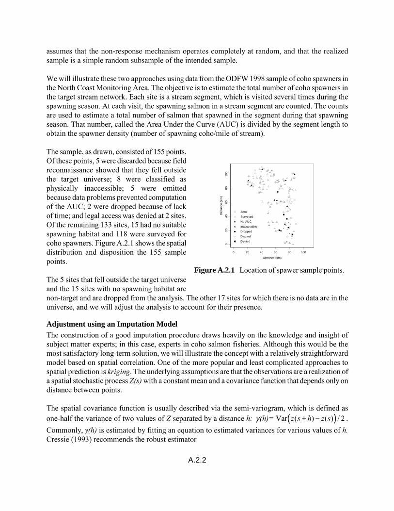
assumes that the non-response mechanism operates completely at random, and that the realized sample is a simple random subsample of the intended sample. We will illustrate these two approaches using data from the ODFW 1998 sample of coho spawners in the North Coast Monitoring Area. The objective is to estimate the total number of coho spawners in the target stream network. Each site is a stream segment, which is visited several times during the spawning season. At each visit, the spawning salmon in a stream segment are counted. The counts are used to estimate a total number of salmon that spawned in the segment during that spawning season. That number, called the Area Under the Curve (AUC) is divided by the segment length to obtain the spawner density (number of spawning coho/mile of stream). The sample, as drawn, consisted of 155 points. Of these points, 5 were discarded because field reconnaissance showed that they fell outside the target universe; 8 were classified as physically inaccessible; 5 were omitted because data problems prevented computation of the AUC; 2 were dropped because of lack of time; and legal access was denied at 2 sites. Of the remaining 133 sites, 15 had no suitable spawning habitat and 118 were surveyed for coho spawners. Figure A.2.1 shows the spatial distribution and disposition the 155 sample points. The 5 sites that fell outside the target universe and the 15 sites with no spawning habitat are non-target and are dropped from the analysis. The other 17 sites for which there is no data are in the universe, and we will adjust the analysis to account for their presence.

Adjustment using an Imputation Model The construction of a good imputation procedure draws heavily on the knowledge and insight of subject matter experts; in this case, experts in coho salmon fisheries. Although this would be the most satisfactory long-term solution, we will illustrate the concept with a relatively straightforward model based on spatial correlation. One of the more popular and least complicated approaches to spatial prediction is kriging. The underlying assumptions are that the observations are a realization of a spatial stochastic process Z(s) with a constant mean and a covariance function that depends only on distance between points. The spatial covariance function is usually described via the semi-variogram, which is defined as one-half the variance of two values of Z separated by a distance h: ( )Var ( ) ( ) / 2(h) = z s h z sγ + − . Commonly, γ(h) is estimated by fitting an equation to estimated variances for various values of h. Cressie (1993) recommends the robust estimator

0 20 40 60 80 100

Distance (km)

020

4060

8010

0

Dis

tanc

e (k

m)

#

#

#

#

#

DeniedDiscardDroppedInaccessibleNo AUCSurveyedZero

#

Figure A.2.1 Location of spawer sample points.

A.2.3

A.2.1 �4

0.5i j

N(h)

1 1 0.494(h) = | z( ) - z( ) _ 0.457 + |s s2 | N(h)| | N(h)|γ

� � � �� �� � � � � ��

�

where N(h) is the collection of data points separated by distance h, and |N(h)| is the number of points in N(h). Where the data don�t occur on a regular spacing, they are grouped into classes. For example, N(hi) might include all pairs of points (sj, sk) such that ( 1) | |i ji h s s ih− ≤ − < . In applying the model, the semi-variogram is usually represented by a parametric equation that captures the spatial dependence of the estimates given by (A.2.1), and also ensures that theoretical constraints are satisfied. For this particular example, we chose an exponential form given by

0 1exp(h) = c (1 - (-c h))γ . To get estimates of c0 and c1, we calculated (A.2.1), using 1 km distance bins, and fitted γ(h) using non-linear last squares. Figure A.2.2 shows the empirical � i( )hγ and the fitted exponential semi-variogram. The estimated coefficients are c0 = 3.63 and c1 = 0.082. The kriging estimator of the response at a point s is a linear combination of the observed responses at the points

r1 2 n, , ..., s s s of the form � ( )

i r

i i s S

z(s) = z sλ∈� where

the weights λi are estimated using the covariance matrix determined by � i(| s - |)sγ (See, for example, Cressie, 1993, pp 120-123). The results of the imputation are given in Table A.2.1. Figure A.2.3 is a perspective plot of the imputation results. Each target population point is located on the plane Z = 0,

020

4060

80100

X (km)

0

20

40

60

80

100

Y (km)

05

1015

2025

30AU

C

1

23

4 56 7

8

910

1112

1314

1516 17N

Figure A.2.3 Perspective plot of observed values (light bar) and imputed values (dark bar).

0 10 20 30 40

Point Separation (km)

02

46

810

Empi

rical

Sem

ivar

iogr

am

Figure A.2.2 Empirical semivariogram and fitted curve � 3.63 exp 0.082(h) = (1 - (- h))γ

A.2.4

Table A.2.1 Imputed values of spawner density Point Number

Status

Spawner Density

1

Denied

0.09

2

Denied

3.72

3

Dropped

0.18

4

Dropped

0

5

Inaccessible

0

6

Inaccessible

0

7

Inaccessible

0.51

8

Inaccessible

6.23

9

Inaccessible

3.74

10

Inaccessible

0.61

11

Inaccessible

5.78

12

Inaccessible

19.72

13

No AUC

0

14

No AUC

0.07

15

No AUC

0

16

No AUC

0

17

No AUC

0

and the spawner density at the point is represented by the height of the bar drawn at the point. Observed values have a gray-shaded bar; imputed values are shown with a black bar.

The sample is an equiprobable sample, so the mean of the sample is an unbiased estimator of the population mean. The mean of the 118 observed values of spawner density is 2.523 fish/mile. The mean of the 17 imputed values is 2.393, so inclusion of the imputed values does not greatly alter the estimated mean value. Each sample represents 6.075 stream miles, the estimated total number of spawning fish represented by the missing data points is (17)(2.393)(6.075) = 247, so that the estimated total number of spawning coho in the North Coast Gene Conservation Area for 1998 is (118)(2.523)(6.075) + 247 = 1809 + 247 = 2056 fish. (For details of the estimation, see Appendices 1 and 3). This result can be compared to the �weight modification� result of 2069 spawners in the North Coast derived below.

Adjustment using weight modification In this section, we develop the details of the simplest weight modification method, although we caution that it is based on assumptions that are almost surely not true. In particular, an explicit assumption is that the portion of the population represented by the non-responsive portion of the sample can reasonably be regarded as a simple random sample from the entire population. If the major reason for non-response is access refusal from generally small landowners, this assumption is probably not tenable. We do not recommend this method, but offer it as a default until a more satisfactory method is available. Suppose the intended sample consisted of np target sites Sp = { 1 2 pns , s , ..., s } with corresponding inclusion densities π(si). Further, suppose that a response was

obtained at nr sites, and let Sr be those sites for which we have a response. The two-stage selection, simple-random-sample assumption is expressed by replacing the inclusion densities π(si) with the

weight-modified inclusion densities πWM(si) given by ri iWM

p

n( ) = ( ) s sn

π π .

Note that because the weight attached to each sample point is the reciprocal of the inclusion density, this correction amounts to increasing the weight of each realized sample point.

A.2.5

Another way of viewing this adjustment is as an assumption that the mean value (e.g., number of spawners per mile of stream) is the same for the response and non-response subpopulations, and applying the estimate based on the realized sample to the entire population. An estimated total number of spawners is obtained by multiplying the estimated mean by the estimated total length of suitable stream habitat. The North Coast MA sample is equiprobable, so π(s) is constant throughout the MA, with a value of 1/6.075 = 0.1646. There were 155 total sites in the sample, of which 20 (5 sites outside the target universe plus 15 sites with no suitable habitat) were non-target, leaving np = 135 target sites. A response was obtained at nr = 118 of the 135 target sites. The modified inclusion probability is then πr = 118/(6.075*135) = 0.1439, giving a weight of 6.950 stream miles to each observed point. The estimated total number of spawners in the North Coast is given by the product of the mean value of spawner density, the number of points, and the weight per point, i.e., (2.523)(118)(6.950) = 2069 spawners in the North Coast MA in 1998.

Estimates of Totals and Means Of the sample of 155 sites, there were 20 non-target and 135 target sites. Letting S0 denote the entire sample, we can estimate the length of stream in the target population using an indicator function and the pi-weighted or Horvitz-Thompson estimator give in Appendix 1 as equation A.1.1. (An indicator function for a condition �indicates� whether or not the condition holds by taking on a value of 1 if the condition is true, and 0 if not. For example, the �target indicator function� Itarget(s) = 1 if s is a site in the target population, and is 0 otherwise.) The estimated total length of target population stream is

� 35 8200

target iT

ii S

( )sI = = (1 )(6.075) = mi .L ( )sπ∈�

Note that this total is summed over the entire sample, reflecting the assumption that the target indicator is defined for every site in the sample, even the inaccessible ones. The variance can be estimated using (A.1.6) as (155)(6.075)2 VSRS( �TL } = 647 giving a standard error of 25.4 mi, and an approximate 95% confidence interval from (A.1.7) of (770, 870) mi for the length of stream in the target population. Alternatively, we can use the neighborhood variance estimator given by (A.1.8): VNB{ �TL } = 434 giving a standard error of 20.8 mi, and an approximate 95% confidence interval from (A.1.7) of (779, 861) mi for the length of stream in the target population. In order to estimate the total number of spawners, we first, for each sampled target site, calculate the observed spawner density zi = (AUC)/(segment length in mi). We then have several ways to proceed.

A.2.6

One is to base the estimate only on observed data, that is, the data for the sites in Sr, and to restrict the reference population. In other words, we redefine the target population to coincide with the population that was actually sampled. In this case, the estimate of the total is

( )� ( )i ri r

iiT

s S s S

z s = = 6.075 z s = 1,809Z ( )si .

π ∈∈��

The sum in this case is over the 118 sites for which we have observed spawner counts. This estimates the total number of spawners in the population that we were able to sample, and we expect it to underestimate the total number in the stream network that we intended to sample. We can adjust by modifying the weight, in effect assuming that the streams that we could not sample are a simple random sample from the population that we could sample. From above, the adjusted weight is 6.950, so that the estimate of the total is

,( )� ( ) ,

i ri r

iT WM i

s S rs S

z sZ = = 6.950 z s = 2 069( )si

π ∈∈

�� .

We can get a conservative variance estimator by using the IRS (A.1.4) approximation, or we can use the approximately unbiased neighborhood estimator (A.1.6). These give, respectively,

Alternatively, we can use an imputation model to predict a value for those sites that are in the target population, but for which we have no observed value. Using the spatial imputation model developed above, we get

,( )� ( ) ,

i pi p

iiT I

s S s S

z s = = 6.075 z s = 2 056Z ( )si

π ∈∈��

Again, we have two possible variance estimators, the IRS and the NB estimator. These yield.

( )� � ,iSRS iT,IIRS( ) = (150) / ( ) = 135 122V szV Z π and � � ,T,INB( ) = 61 579 V Z .

Note that although the weight adjustment and the imputation model give nearly the same estimated total, the imputed total has a much smaller variance. To some extent, the agreement between the two estimated totals supports the �missing at random� assumption of the weight adjustment technique. The smaller variance of the imputed total is due to the stronger assumption incorporated via the spatial model. The lower variance is a valid estimator, provided the imputation model, i.e., the assumption of strong spatial pattern, is �correct� in the sense that it is a good description of reality.

( )� � iSRS r iT,WAIRS( ) = (118 ) / ( ) = 157,911V szV Z π and � � ,T,WANB( ) = 80 598 .V Z

A.2.7

We illustrate the estimation of a mean by estimating the average spawner density. By definition, the average density is the total number of spawners divided by the total stream miles. If the stream frame were perfect, it would seem that we could get the total number of stream miles from frames information, i.e., from the GIS coverage. However, it turns out that it usually better to estimate the total miles rather than use the frame total. In particular, if the frame is imperfect, (as it is the present case), if the sample size is random, or if the survey uses variable probability, then it is preferable to use an estimated total. In these three cases, there will generally be some positive correlation between the estimated response total and the estimated size of the population, e.g., between the estimated number of spawners and the estimated total stream miles. Because of the positive correlation, the ratio of the two estimated totals will generally be more precise than the ratio of the estimated response total to the true population size. Proceeding as above, the estimated mean spawner density is

�� spawners/mile.�

T, i

T

2056ZD = = = 2.51 820L

The appropriate variance estimator for the ratio estimator is obtained using ��i(z - D) in place of zi in

the neighborhood estimator, and then dividing the result by � 2TL . Because the North Coast sample is

equi-probable, this will be the same as � � � 2T, I TNB( )/V Z L . Thus,

,�� � � � 2T, I TNB NB 2

61 579(D) = ( )/ = = 0.0916V V Z L 820

Subpopulation Analyses The estimation equations (A.1.1) through (A.1.9) can be used to estimate the proportion of a population that meets some criteria or falls within some category. For example, we may be interested in the proportion of the North-Coast target population that is 1st order streams, or the proportion with spawner density less than x. To do this, we form a new response variable that takes on the value 1 if a sample site meets the criteria or is in the category, and 0 otherwise. We call this new response the indicator variable for the criteria or category. For the category {stream order = 1st}, the indicator

variable is st

sti

order i1

1, if on order segments 1( ) = s0, otherwise

I���

. The mean value of the indicator variable is the

proportion we want, and we estimate it and its variance using the same method as for any other

mean. Thus, for example, 1

1

( ) ( )�

( )

st

st

i iorderi

orderi

i

I s w sp

w s=�

� would give the estimated proportion of 1st

order streams in the target population.

A.2.8

To illustrate a subpopulation analysis, split the data on latitude, and define the "northern" subpopulation as all stream miles north of latitude 45.5°. The corresponding indicator variable is

, if latitude at > .( ) =

, otherwisei

N i

1 s 45 5I s

0���

. The indicator variable is defined for all target streams, not just

those for which we have spawner counts. We get our best estimate of total northern stream length by applying the indicator variable to the 135 target sites, not just to those with spawner counts. Let St denote the set of site ID's for the 135 target sites, and SN denote the set of site ID's for the target sites in the northern subset. There are 100 sample points in SN, so the estimated length of streams in the northern subpopulation is

� . mi .i t N

N iT, N

i i i s S S

( ) 1sI = = = (100 )(6.075) = 607 5L ( ) ( )s sπ π∈ ∈� �

Note that we use the un-adjusted inclusion density, not the inclusion density adjusted for non-response. Again, one estimator variance uses (A.1.6), giving (135)(6.075)2 VSRS{IN} = 964. This estimate is based on the assumption that the indicator value is the result of a simple random sample, and in this case is very conservative. The indicator value is actually the result of a spatially constrained sample selected from a population with a very strong spatial pattern. The sampling technique will always result in nearly 100 samples in the northern subpopulation; the only variation will be in those few samples that are near the 45.5° latitude line. The neighborhood variance estimator (A.1.8) reflects the reduced variance resulting from the strong spatial pattern in the population coupled with the spatially constrained sampling: � � .T,NNB( ) = 47 8 .V L

The estimated total number of spawners in the northern half is computed in the same manner as the overall North Coast total, except that the response is multiplied by the �northern� indicator function. We illustrate using the imputed values for spawner counts:

, ,( ) ( )� . ( )

( )i p i N

N i iT I N i

s S s Si

I s z sZ 6 075 z s 1819sπ∈ ∈

= = =� � .

The neighborhood variance estimator is the best choice. It should be applied to only those samples in SN, i.e.,

{ }, ,( )� �( )

i j i iN N k N

2

j ki j ikT I NNB

S D ( ) s D ( )j ks s s s

z(s ) z s( ) = - wwV Z (s ) sπ π∈ ∈ ∈� � � ,

where the neighborhood DN(sj) is computed with respect to SN, not S0. Technically, this estimator is conditional on the sample size in the northern subpopulation being fixed at 100. An unconditional estimator would account for the increased variance resulting from the random sample size. However,

A.2.9

there should be little variation in achieved sampled size with the spatially balanced design because the northern subpopulation is spatially contiguous. There are two proportions that we might have some interest in for this subpopulation: the proportion of the total stream length in the population, and the proportion of total spawners. These are calculated as ratios of the corresponding estimates:

, � .proportion of stream length in north = = = = .� .T N

T

607 5 100L 0 741819 45 135L

and

, ,

,

�proportion of spawners in north = = = .�

T I N

T I

Z 1819 0 8852056Z

.

Note that because the North-Coast sample is equi-probable, the weighted estimated proportion of extent, i.e., the length ratio, reduces to a simple ratio of counts.

Cumulative Distribution Function (cdf) Estimation We can view the computation of the cdf as calculating proportions for a sequence of subpopulations, where we define the subpopulations by the level of response. We pick a set of numbers x1, ..., xm to span the range of the response, and then calculate proportions for the m subpopulations defined by the criteria {response ≤ xj}. The resulting sequence of proportions is the cdf as a function of x. We illustrate with spawner density as the response. For the example, we�ll use the imputed values of spawner density for the target sites with missing data. The range of spawner density is {0, 32.1). We will calculate the cdf at 18 evenly spaced points {0, 2, 4, �, 34}. We show the details of the computation of the first two points on the cdf, and then exhibit the remainder. The first point is at the spawner density of 0, and represents the fraction of stream with no spawners. We form the indicator function,

1 0(z ) (z )x (z(s)) = (z(s))I I≤ = and use (A.1.10) to get

( ) ( )( ) ( ) . ( )� ( ) .

( ) ( )( . )

z s 0 i i z s 0 ii i

zi

i

I s w s 6 075 I s80F 0 0 5926

w s 135 6 075 135

= =

= = = =� �

�.

For 2ix = , we form the indicator function

2(z ) (z 2)x (z(s)) = (z(s))I I≤ ≤ , and, following (A.1.10), calculate the proportion

( ) ( )

( )

( ) ( ) . ( )� ( ) .

( ) ( ) ( . )( )

z s 2 i i z s 2 ii i

zz s 0 i i

i

I s w s 6 075 I s98F 2 0 7259

I s w s 6 075 135 135

≤ ≤

>

= = = =� �

�

A.2.10

Again, because we have an equi-probable sample, and we are estimating proportion of extent in a class, the estimate reduces to a ratio of counts. We take advantage of this in calculating the rest of the points on the cdf by simply counting the number of sample points with spawner density less than or equal to xj, and then dividing by 135:

jnumber of samples with spawner density x� .jZ( ) = xF 135≤

This is a ratio estimator; so we calculate the neighborhood variance estimator using (A.1.8) with �

j(z ) jx i Z(s ) - ( )xI F≤ in place of z(si). The IRS variance estimator reduces to � �( )( ( ))� �( ( )) z z

IRS zF x 1 F xV F x

135−= . We calculate confidence intervals as before. The estimated cdf and

confidence limits based on both variance estimators are exhibited in Table A.2.2 and plotted in Figure A.2.4.

0 10 20 30

Spawner Density,fish/m ile

0.0

0.2

0.4

0.6

0.8

1.0

Cum

ulat

ive

Prop

ortio

n <=

x

95% IRS Confidence Lim its

Estimated cdf

95% NB Confidence Lim its

Figure A.2.4 Cumulative distribution function of spawner density.

A.2.11

Table A.2.2 Estimated cumulative distribution function of spawner density. X

� Z(x)F

IRS 95% CI

NB 95% CI

0 0.593 0.509 0.676 0.532 0.653 2 0.726 0.65 0.801 0.67 0.782 4 0.815 0.749 0.881 0.763 0.867 6 0.844 0.783 0.906 0.796 0.893 8 0.889 0.836 0.942 0.847 0.931 10 0.911 0.863 0.959 0.875 0.948 12 0.948 0.911 0.986 0.924 0.972 14 0.963 0.931 0.995 0.941 0.985 16 0.963 0.931 0.995 0.941 0.985 18 0.963 0.931 0.995 0.941 0.985 20 0.978 0.953 1.000 0.957 0.999 22 0.985 0.965 1.000 0.968 1.000 24 0.993 0.978 1.000 0.980 1.000 26 0.993 0.978 1.000 0.980 1.000 28 0.993 0.978 1.000 0.980 1.000 30 0.993 0.978 1.000 0.980 1.000 32 0.993 0.978 1.000 0.980 1.000 34 1 1.000 1.000 1.000 1.000

A.2.12

References Cressie, N.A.C. 1993. Statistics for Spatial Data John Wiley & Sons. New York. Kalton, G., and Kasprzyk, D. 1986. The Treatment of Missing Survey Data. Survey Methodology 12, 1-16.

A.3.1

Appendix 3: 1998 North Coast Coho Spawner Data Site Number Status Latitude Longitude AUC Length (Miles) 1 Denied 45.19430 123.8978 NA 0.49 2 Denied 45.44998 123.7409 NA 0.25 3 Discard 45.21305 123.8473 NA NA 4 Discard 45.33139 123.8639 NA NA 5 Discard 45.27587 123.7353 NA NA 6 Discard 45.35199 123.8309 NA NA 7 Discard 45.91201 123.8824 NA NA 8 Dropped 45.39655 123.7970 NA 1.28 9 Dropped 45.74142 123.6335 NA 0.50 10 Inaccessible 45.63238 123.6161 NA NA 11 Inaccessible 45.63726 123.5713 NA NA 12 Inaccessible 45.55813 123.8035 NA NA 13 Inaccessible 46.03275 123.3469 NA 1.10 14 Inaccessible 45.88560 123.0917 NA NA 15 Inaccessible 45.82732 123.1500 NA NA 16 Inaccessible 45.96747 123.9436 NA 0.33 17 Inaccessible 45.88868 123.7801 NA NA 18 No AUC 45.28482 123.8226 NA 0.86 19 No AUC 45.32687 123.7618 NA 0.81 20 No AUC 45.24856 123.6659 NA 1.10 21 No AUC 45.25117 123.6590 NA 1.10 22 No AUC 45.24191 123.6899 NA 0.92 23 Surveyed 45.07003 123.9092 0 0.25 24 Surveyed 45.14209 123.8837 5 0.46 25 Surveyed 45.08865 123.8458 0 0.43 26 Surveyed 45.08115 123.8427 0 0.52 27 Surveyed 45.10587 123.7978 0 0.76 28 Surveyed 45.10403 123.7887 0 0.17 29 Surveyed 45.08813 123.7587 0 1.14 30 Surveyed 45.09421 123.7847 0 1.40 31 Surveyed 45.23323 123.9242 0 1.48 32 Surveyed 45.17754 123.8863 0 0.80 33 Surveyed 45.17145 123.8021 0 1.34 34 Surveyed 45.28146 123.8424 0 0.62 35 Surveyed 45.31145 123.7836 0 1.06 36 Surveyed 45.25946 123.8038 0 1.02 37 Surveyed 45.25472 123.6419 0 0.81 38 Surveyed 45.23841 123.5913 0 1.03 39 Surveyed 45.27449 123.5743 0 1.42 40 Surveyed 45.31051 123.4792 1 1.14 41 Surveyed 45.31665 123.4720 5 0.89 42 Surveyed 45.39421 123.8023 0 0.50 43 Surveyed 45.35359 123.5445 7 0.64 44 Surveyed 45.36397 123.5191 0 0.63 45 Surveyed 45.35406 123.4594 0 0.86 46 Surveyed 45.35648 123.6154 0 0.71 47 Surveyed 45.46830 123.4561 0 0.91 48 Surveyed 45.46748 123.4570 0 0.91 49 Surveyed 45.48418 123.7338 5 0.77 50 Surveyed 45.54923 123.4967 1 0.91 51 Surveyed 45.55271 123.4900 0 0.28 52 Surveyed 45.60014 123.6111 0 0.29 53 Surveyed 45.58581 123.5158 0 0.42 54 Surveyed 45.60914 123.4658 0 0.86

A.3.2

Site Number Status Latitude Longitude AUC Length (Miles) 55 Surveyed 45.58957 123.4523 0 0.71 56 Surveyed 45.61617 123.3500 9 0.97 57 Surveyed 45.50037 123.8110 0 0.71 58 Surveyed 45.53034 123.8331 0 0.86 59 Surveyed 45.60855 123.7536 0 0.54 60 Surveyed 45.61549 123.7516 0 1.51 61 Surveyed 45.61973 123.7293 0 1.24 62 Surveyed 45.61879 123.6884 0 0.99 63 Surveyed 45.62025 123.6948 0 1.20 64 Surveyed 45.61917 123.6772 0 1.20 65 Surveyed 45.59070 123.8743 0 0.90 66 Surveyed 45.61427 123.8898 0 0.53 67 Surveyed 45.60534 123.8454 0 1.24 68 Surveyed 45.63071 123.8102 0 1.44 69 Surveyed 45.76182 123.9041 0 0.34 70 Surveyed 45.77149 123.8947 0 1.06 71 Surveyed 45.78002 123.8606 19 1.59 72 Surveyed 45.74860 123.8374 0 0.90 73 Surveyed 45.76048 123.8396 0 0.34 74 Surveyed 45.78482 123.8487 0 0.81 75 Surveyed 45.84114 123.7666 11 0.80 76 Surveyed 45.78292 123.7183 0 0.89 77 Surveyed 45.77242 123.6593 0 0.44 78 Surveyed 45.81561 123.6959 3 0.87 79 Surveyed 45.82308 123.6844 6 1.25 80 Surveyed 45.72347 123.8344 0 0.18 81 Surveyed 45.69368 123.8445 0 0.60 82 Surveyed 45.66992 123.8384 0 1.24 83 Surveyed 45.64133 123.8629 0 0.34 84 Surveyed 45.86801 123.5994 0 1.30 85 Surveyed 45.86667 123.6364 11 1.24 86 Surveyed 45.89001 123.6195 3 1.18 87 Surveyed 45.87740 123.6526 1 1.03 88 Surveyed 45.89507 123.6411 3 1.00 89 Surveyed 45.89949 123.4524 14 1.49 90 Surveyed 45.93938 123.5078 0 1.15 91 Surveyed 45.95246 123.5052 0 1.35 92 Surveyed 45.99495 123.4913 0 1.14 93 Surveyed 46.01345 123.5114 0 0.35 94 Surveyed 46.01992 123.5261 0 1.03 95 Surveyed 45.95701 123.5686 0 1.14 96 Surveyed 45.97241 123.5621 9 0.86 97 Surveyed 45.96687 123.4365 0 1.40 98 Surveyed 46.00674 123.4334 0 0.80 99 Surveyed 46.02460 123.4538 2 1.29 100 Surveyed 45.94889 123.3204 0 0.84 101 Surveyed 45.93008 123.3071 0 0.85 102 Surveyed 45.90356 123.3361 0 1.18 103 Surveyed 46.04367 123.3795 2 0.30 104 Surveyed 46.06490 123.3387 16 0.76 105 Surveyed 46.00310 123.3307 0 1.03 106 Surveyed 46.03140 123.3005 0 0.51 107 Surveyed 46.01707 123.2140 0 1.38 108 Surveyed 45.97981 123.2163 0 1.15 109 Surveyed 45.92491 123.2455 2 1.50

A.3.3

Site Number Status Latitude Longitude AUC Length (Miles) 110 Surveyed 45.94704 123.0968 3 1.60 111 Surveyed 45.94067 123.1771 1 1.00 112 Surveyed 45.91557 123.1824 8 1.20 113 Surveyed 45.87063 123.0772 2 0.51 114 Surveyed 45.83841 123.0758 1 1.03 115 Surveyed 45.83720 123.0876 0 0.96 116 Surveyed 45.85954 123.3083 4 1.14 117 Surveyed 45.87376 123.3112 4 1.14 118 Surveyed 45.88000 123.3605 8 1.30 119 Surveyed 45.83926 123.3799 1 1.67 120 Surveyed 45.81071 123.4600 2 0.97 121 Surveyed 45.77169 123.4338 0 1.24 122 Surveyed 45.81495 123.1343 0 0.65 123 Surveyed 45.81069 123.1837 0 0.28 124 Surveyed 45.80759 123.1796 1 1.00 125 Surveyed 45.80120 123.2950 0 1.20 126 Surveyed 45.79715 123.3124 0 1.26 127 Surveyed 45.78129 123.3630 8 1.40 128 Surveyed 45.74407 123.3064 8 0.63 129 Surveyed 45.73491 123.3407 4 1.33 130 Surveyed 45.73672 123.2846 3 1.00 131 Surveyed 45.72476 123.2857 1 1.20 132 Surveyed 45.76159 123.9595 0 1.14 133 Surveyed 45.98170 123.9128 1 1.24 134 Surveyed 45.96662 123.9203 7 1.03 135 Surveyed 45.92446 123.9293 13 1.14 136 Surveyed 45.89161 123.8829 0 0.51 137 Surveyed 45.91810 123.8025 28 1.20 138 Surveyed 45.88890 123.7491 4 1.11 139 Surveyed 45.88172 123.7516 26 0.81 140 Surveyed 45.90911 123.7311 14 0.77 141 Zero 45.19656 123.9037 0 0.50 142 Zero 45.32848 123.9635 0 0.50 143 Zero 45.40703 123.8742 0 0.50 144 Zero 45.33989 123.7760 0 0.50 145 Zero 45.51399 123.8540 0 0.50 146 Zero 45.63582 123.9388 0 0.50 147 Zero 45.79270 123.6657 0 0.50 148 Zero 45.86428 123.5917 0 0.50 149 Zero 45.94048 123.5444 0 0.50 150 Zero 45.91384 123.3062 0 0.50 151 Zero 45.86676 123.1258 0 0.50 152 Zero 45.85109 123.3133 0 0.50 153 Zero 45.85098 123.1611 0 0.50 154 Zero 45.83745 123.1882 0 0.50 155 Zero 45.92331 123.9398 0 0.50

A.4.1

Appendix 4: Annotated Splus Commands and Function Definitions Used in Appendix 2

Splus commands to impute missing values using spatial interpolation via kriging: Splus commands are in italics; comments are in regular font. Initially, the North Coast 1998 data are in stored in an Splus data frame (nc.spwn.df) with 155 rows and 10 columns. Column identifiers are: names(nc.spwn.df) [1] "Year" "Status" "Latitude" "Longitude" [5] "AUC" "Miles" "x" "y" [9] "prb" "SpwnDen" The xy coordinates are in kilometers. Set up pointers to pick out all pairs of the 133 �good� data points. �kdx.lwr.fcn� is given below. idx <- rep(1:133, 133) jdx <- rep(1:133, rep(133, 133)) gpdx <- idx < jdx jdx <- jdx[gpdx] idx <- idx[gpdx] kord <- order(kdx.lwr.fcn(idx, jdx, 133)) idx <- idx[kord] jdx <- jdx[kord] Pick out the sites with non-missing AUC, compute spawner density, and get (x, y) coordinates for good points: gp <- !is.na(nc.spwn.df$AUC) sp.den <- nc.spwn.df$SpwnDen[gp] s <- cbind(nc.spwn.df$x[gp], nc.spwn.df$y[gp]) Calculate the empirical semivariogram . First, assign every pair of points to a distance class. The Splus function �dist(s)� calculates all possible distances between points; �ceiling()� is used to assign distance classes. The distance class i includes all pairs of points separated by at least (i-1) kilometers but no more than i kilometers. The vectors �idx� and �jdx� identify the points corresponding to the distance class ds.cl, that is, the points idx[i] and jdx[i] belong to distance class ds.cl[i]. Maximum separation distance was limited to 35 kilometers based on an examination of the empirical semivariogram.

A.4.2

ds.cl <- ceiling(dist(s)) svr.sp.den <- numeric(35) for(i in 1:35) {

gpi <- ds.cl == i svr.sp.den[i] <- (sum(sqrt(abs(sp.den[idx[gpi]] - sp.den[jdx[gpi]])))/sum(gpi))^

4/(0.457 + 0.494/sum(gpi))/2 }

Fit the exponential form of a theoretical semivariogram to the empirical semivariogram using non-linear least-squares. The �param� commands provide starting values for the iterative fitting algorithm �nls� ds.ft <- 1:35 - 0.5 sp.den.ft.df <- data.frame(ds.ft, svr.sp.den) param(sp.den.ft.df, "a0") <- 4 param(sp.den.ft.df, "a1") <- 0.15 sp.den.gam.ft <- nls(svr.sp.den ~ a0 * (1 - exp( - a1 * ds.ft)), sp.den.ft.df) svr.sp.den.ft <- sp.den.gam.ft$parameters[1]*(1-exp(-sp.den.gam.ft$parameters[2]*ds.ft)) Calculate the spatial covariance matrix used in the kriging predictor. �gam.fcn� is given below. The Splus function �solve� computes the matrix inverse. gam.sp.den <- gam.fcn(s, sp.den.gam.ft$parameters) gam.sp.den.inv <- solve(gam.sp.den) Calculate the kriging predictor for the missing values in the target domain. �krig.fcn� is given below. gp.msng <- is.na(nc.spwn.df$AUC) & nc.spwn.df$Status != "Discard" sp.den.pred <- krig.fcn(sp.den.gam.ft$parameters, gam.sp.den.inv, sp.den, s, nc.spwn.df$x[gp.msng], nc.spwn.df$y[gp.msng]) sp.den.pred<- pmax(0, sp.den.pred)

Function listings for spatial imputation dist2full.fcn function(dis) { # converts a lower triangular matrix stored as a vector into a full matrix

A.4.3

n <- attr(dis, "Size") full <- matrix(0, n, n) full[lower.tri(full)] <- dis full + t(full)

} gam.fcn function(s, cf) {

dst <- dist(s) gij <- cf[1] * (1 - exp( - cf[2] * dst)) gam <- dist2full.fcn(gij) diag(gam) <- 0 gam

} kdx.lwr.fcn function(i, j, n = 50.) { # computes the element index of a lower triangular matrix stored as a vector, # given the dimension of the matrix & the row & column indices. The inverse # function is "tri.ndx.fcn" # # this function must have i < j. # n * (i - 1.) + j - i - (i * (i - 1.))/2. } krig.fcn function(cf, gaminv, z, s, xpred, ypred) { # # calculates kriging predictor using exponential semivariogram # cf - coeficients of semivariogram # gaminv - inverse of gamman MAtrix # z - observed response # s - (x,y) coordinates of observed response # (xpred, ypred) - (x,y) coordinates of predictions #

A.4.4

lnprd <- length(xpred) pred <- numeric(lnprd) one <- rep(1, (dim(gaminv))[1]) for(i in 1:lnprd) {

lcgm <- cf[1] * (1 - exp( - cf[2] * sqrt((s[, 1] - xpred[i])^2 + (s[, 2] - ypred[i])^2)))

lm <- (lcgm + (one * (1 - t(one) %*% gaminv %*% lcgm))/ (t(one) %*% gaminv %*% one)) %*% gaminv

pred[i] <- sum(lm * z) } pred

}

Splus Commands for Computing Means, Totals, and CDFs Splus commands are in italics; comments are in regular font. The North Coast 1998 data are in stored in an Splus data frame (nc.spwn.df) with 155 rows and 11 columns. SpwnDen.Imp contains both observed spawner density and imputed values from spatial imputation. Column identifiers are: names(nc.spwn.df) [1] "Year" "Status" "Latitude" "Longitude" [5] "AUC" "Miles" "x" "y" [9] "prb" "SpwnDen" "SpwnDen.Imp" Below are the commands that reproduce the results given in Appendix 2. The function odfw.lcl.mean.fcn calculates estimated total number of spawners in the population that was sampled. Function listing given below. odfw.lcl.mean.fcn(nc.spwn.df[!is.na(nc.spwn.df$AUC), c(7,8,9,10)]) Total V-total-irs V-total-nb Mean V-mean-irs V-mean-nb 1808.627 120644.6 61577.01 2.522988 0.2347688 0.1198259 Adjust the weight by a factor of 135/118 and re-compute. odfw.lcl.mean.fcn(nc.spwn.df[!is.na(nc.spwn.df$AUC), c(7,8,9,10)]*rep(c(1,1,118/135,1),rep(118,4))) Total V-total-irs V-total-nb Mean V-mean-irs V-mean-nb 2069.192 157910.7 80597.6 2.522988 0.2347688 0.1198259

A.4.5

Use imputed values for spawner density: odfw.lcl.mean.fcn(nc.spwn.df[!is.na(nc.spwn.df$SpwnDen.Imp), c(7,8,9,11)]) Total V-total-irs V-total-nb Mean V-mean-irs V-mean-nb 2055.719 135121.9 61579.2 2.50656 0.2008882 0.09155093 To computed the cdf using imputed spawner density: round(odfw.lcl.cdf.fcn nc.spwn.df[!is.na(nc.spwn.df$SpwnDen.Imp), c(7,8,9,11)] , nc.zrng), 5) z CDF V-irs V-nb LCL-irs LCL-nb UCL-irs UCL-nb [1,] 0 0.59259 0.00180 0.00095 0.67579 0.65295 0.50940 0.53224 [2,] 2 0.72593 0.00148 0.00081 0.80145 0.78183 0.65040 0.67002 [3,] 4 0.81481 0.00113 0.00071 0.88059 0.86705 0.74904 0.76258 [4,] 6 0.84444 0.00098 0.00061 0.90581 0.89273 0.78308 0.79616 [5,] 8 0.88889 0.00074 0.00045 0.94210 0.93067 0.83568 0.84710 [6,] 10 0.91111 0.00060 0.00035 0.95930 0.94754 0.86293 0.87468 [7,] 12 0.94815 0.00037 0.00015 0.98569 0.97182 0.91061 0.92448 [8,] 14 0.96296 0.00027 0.00012 0.99494 0.98459 0.93099 0.94134 [9,] 16 0.96296 0.00027 0.00012 0.99494 0.98459 0.93099 0.94134 [10,] 18 0.96296 0.00027 0.00012 0.99494 0.98459 0.93099 0.94134 [11,] 20 0.97778 0.00016 0.00012 1.00000 0.99881 0.95282 0.95675 [12,] 22 0.98519 0.00011 0.00008 1.00000 1.00000 0.96473 0.96790 [13,] 24 0.99259 0.00005 0.00004 1.00000 1.00000 0.97807 0.97974 [14,] 26 0.99259 0.00005 0.00004 1.00000 1.00000 0.97807 0.97974 [15,] 28 0.99259 0.00005 0.00004 1.00000 1.00000 0.97807 0.97974 [16,] 30 0.99259 0.00005 0.00004 1.00000 1.00000 0.97807 0.97974 [17,] 32 0.99259 0.00005 0.00004 1.00000 1.00000 0.97807 0.97974 [18,] 34 1.00000 0.00000 0.00000 1.00000 1.00000 1.00000 1.00000

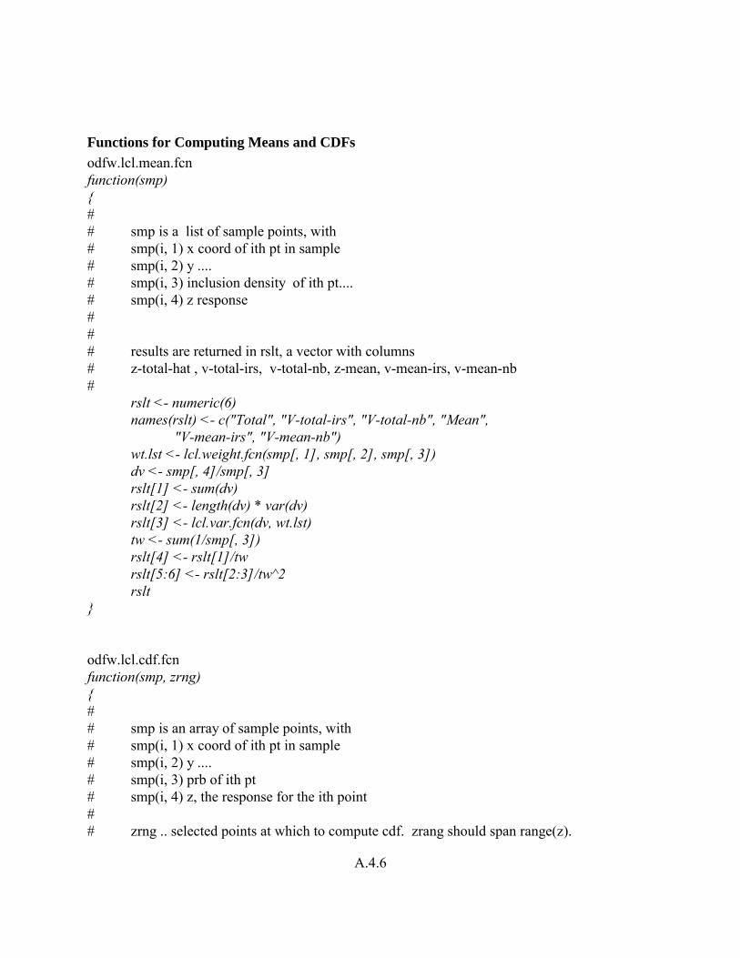
A.4.6

Functions for Computing Means and CDFs odfw.lcl.mean.fcn function(smp) { # # smp is a list of sample points, with # smp(i, 1) x coord of ith pt in sample # smp(i, 2) y .... # smp(i, 3) inclusion density of ith pt.... # smp(i, 4) z response # # # results are returned in rslt, a vector with columns # z-total-hat , v-total-irs, v-total-nb, z-mean, v-mean-irs, v-mean-nb #

rslt <- numeric(6) names(rslt) <- c("Total", "V-total-irs", "V-total-nb", "Mean",

"V-mean-irs", "V-mean-nb") wt.lst <- lcl.weight.fcn(smp[, 1], smp[, 2], smp[, 3]) dv <- smp[, 4]/smp[, 3] rslt[1] <- sum(dv) rslt[2] <- length(dv) * var(dv) rslt[3] <- lcl.var.fcn(dv, wt.lst) tw <- sum(1/smp[, 3]) rslt[4] <- rslt[1]/tw rslt[5:6] <- rslt[2:3]/tw^2 rslt

} odfw.lcl.cdf.fcn function(smp, zrng) { # # smp is an array of sample points, with # smp(i, 1) x coord of ith pt in sample # smp(i, 2) y .... # smp(i, 3) prb of ith pt # smp(i, 4) z, the response for the ith point # # zrng .. selected points at which to compute cdf. zrang should span range(z).

A.4.7

# # results are returned in rslt, an MAtrix with columns # zrng, cdf-hat, V-irs, V-nb, lwr 95% CL's for IRS & NB, upper 95% CL's #

m <- length(zrng) rslt <- matrix(0, m, 8) dimnames(rslt) <- list(NULL, c("z", "CDF", "V-irs", "V-nb",

"LCL-irs", "LCL-nb", "UCL-irs", "UCL-nb")) rslt[, 1] <- zrng n <- dim(smp)[1] ym <- matrix(rep(zrng, n), nrow = n, byrow = T) z <- smp[, 4] prb <- smp[, 3] dv <- z/prb wt <- 1/prb tw <- sum(wt) zm <- matrix(rep(z, m), nrow = n) wm <- matrix(rep(wt, m), nrow = n) cm <- ifelse(zm <= ym, 1, 0) zcdf <- rslt[, 2] <- apply(ifelse(zm <= ym, wm, 0), 2, sum)/tw dvm <- (cm - matrix(rep(zcdf, n), nrow = n, byrow = T)) * wm wt.lst <- lcl.weight.fcn(smp[, 1], smp[, 2], prb) rslt[, 3] <- (n * apply(dvm, 2, var))/tw^2 rslt[, 4] <- apply(dvm, 2, lcl.var.fcn, wt.lst)/tw^2 rslt[, 5:6] <- pmin(1, rslt[, 2] + 1.96 * sqrt(rslt[, 3:4])) rslt[, 7:8] <- pmax(0, rslt[, 2] - 1.96 * sqrt(rslt[, 3:4])) rslt

} lcl.weight.fcn function(x, y, prb) { # computes weighting matrix for local variance estimator # given vectors of x, y, and inclusion probability. # # weights are forced to be doubly stochastic # so that zb is a true local average, and conserves total. #

ldv <- length(x) # # pick out the 4 closest points to each point

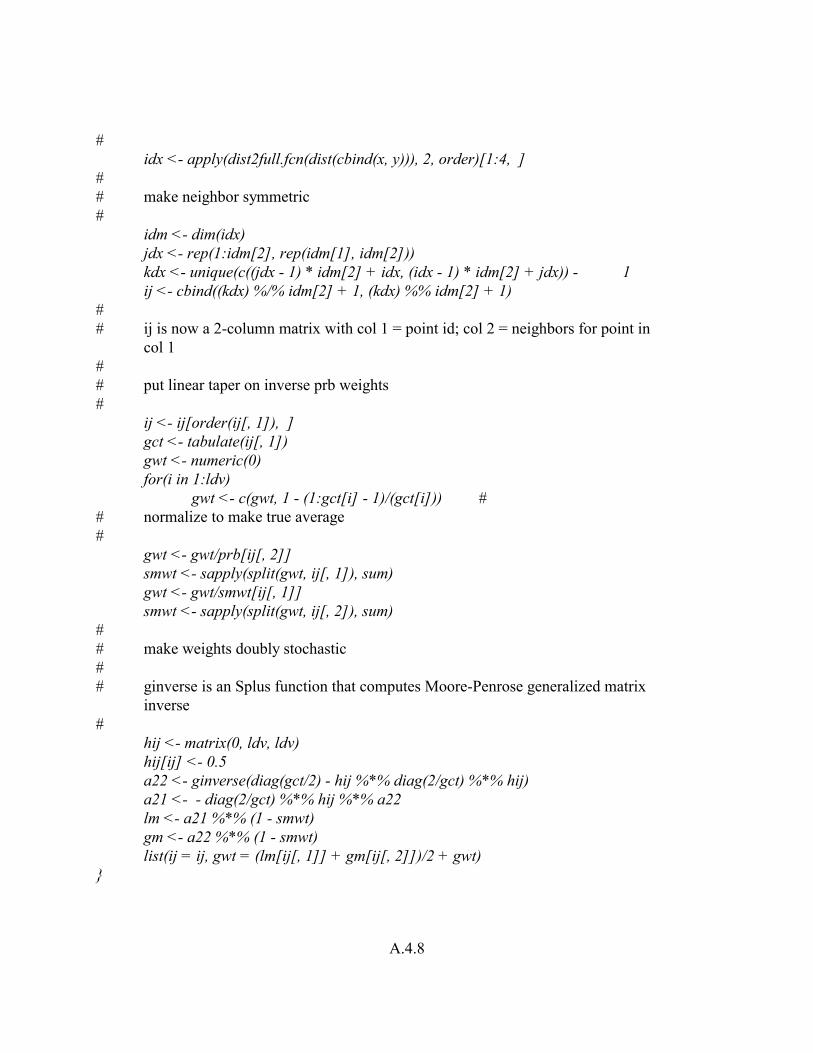
A.4.8

# idx <- apply(dist2full.fcn(dist(cbind(x, y))), 2, order)[1:4, ]

# # make neighbor symmetric #

idm <- dim(idx) jdx <- rep(1:idm[2], rep(idm[1], idm[2])) kdx <- unique(c((jdx - 1) * idm[2] + idx, (idx - 1) * idm[2] + jdx)) - 1 ij <- cbind((kdx) %/% idm[2] + 1, (kdx) %% idm[2] + 1)

# # ij is now a 2-column matrix with col 1 = point id; col 2 = neighbors for point in

col 1 # # put linear taper on inverse prb weights #

ij <- ij[order(ij[, 1]), ] gct <- tabulate(ij[, 1]) gwt <- numeric(0) for(i in 1:ldv)

gwt <- c(gwt, 1 - (1:gct[i] - 1)/(gct[i])) # # normalize to make true average #

gwt <- gwt/prb[ij[, 2]] smwt <- sapply(split(gwt, ij[, 1]), sum) gwt <- gwt/smwt[ij[, 1]] smwt <- sapply(split(gwt, ij[, 2]), sum)

# # make weights doubly stochastic # # ginverse is an Splus function that computes Moore-Penrose generalized matrix

inverse #

hij <- matrix(0, ldv, ldv) hij[ij] <- 0.5 a22 <- ginverse(diag(gct/2) - hij %*% diag(2/gct) %*% hij) a21 <- - diag(2/gct) %*% hij %*% a22 lm <- a21 %*% (1 - smwt) gm <- a22 %*% (1 - smwt) list(ij = ij, gwt = (lm[ij[, 1]] + gm[ij[, 2]])/2 + gwt)

}

A.4.9

"lcl.var.fcn"<- function(dv, wt.lst) { # calculates local variance estimator # dv is (obs - est mean)/prb # wt.lst is list with ij & weight matrix from weight lcl.weight.fcn # # #

zb <- sapply(split(dv[wt.lst$ij[, 2]] * wt.lst$gwt, wt.lst$ij[, 1]), sum)

sum(wt.lst$gwt * (dv[wt.lst$ij[, 2]] - zb[wt.lst$ij[, 1]])^2) }