Focus: A Constraint for Concentrating High Costs

Thierry Petit

To cite this version:

Thierry Petit. Focus: A Constraint for Concentrating High Costs. Proc. First InternationalWorkshop on Search Strategies and Non-standard Objectives, (CPAIOR-SSNOW’12), May2012, Nantes, France, France. 2012. <hal-00753673>

HAL Id: hal-00753673

https://hal.inria.fr/hal-00753673

Submitted on 26 Nov 2012

HAL is a multi-disciplinary open accessarchive for the deposit and dissemination of sci-entific research documents, whether they are pub-lished or not. The documents may come fromteaching and research institutions in France orabroad, or from public or private research centers.

L’archive ouverte pluridisciplinaire HAL, estdestinee au depot et a la diffusion de documentsscientifiques de niveau recherche, publies ou non,emanant des etablissements d’enseignement et derecherche francais ou etrangers, des laboratoirespublics ou prives.

FOCUS: A Constraint for Concentrating High Costs

Thierry Petit

TASC (Mines Nantes, LINA, CNRS, INRIA),

4, Rue Alfred Kastler, FR-44307 Nantes Cedex 3, France.

Thierry.Petit@mines-nantes.fr

Abstract. Many Constraint Programming models use integer cost variables ag-

gregated in an objective criterion. In this context, some constraints involving

exclusively cost variables are often imposed. Such constraints are complemen-

tary to the objective function. They characterize the solutions which are accept-

able in practice. This paper deals with the case where the set of costs is a se-

quence, in which high values should be concentrated in a few number of areas.

Representing such a property through an search heuristic may be complex and

overall not precise enough. To solve this issue, we introduce a new constraint,

FOCUS(X, yc , len , k), where X is a sequence of n integer variables, yc an in-

teger variable, and len and k are two integers. To satisfy FOCUS, the minimum

number of distinct sub-sequences of consecutive variables in X , of length at most

len and that involve exclusively values strictly greater than k, should be less than

or equal to yc . We present two examples of problems involving FOCUS. We pro-

pose a complete filtering algorithm in O(n) time complexity.

1 Introduction

Encoding optimization problems using Constraint Programming (CP) often requires to

define cost variables, which are aggregated in an objective criterion. To be compara-

ble one another, those variables have generally a totally ordered domain. They can be

represented by integer variables. In this context, some constraints on cost variables are

complementary to the objective function. They characterize the solutions which are ac-

ceptable in practice. For instance, to obtain balanced solutions several approaches have

been proposed: Balancing constraints based on statistics [6, 11], as well as classical or

dedicated cardinality constraints when the set of costs is a sequence [9, 8]. Some ap-

plications of these techniques are presented in [12, 7]. Representing such constraints,

as well as solving efficiently the related problems, form an important issue because

real-life problems are rarely “pure”. In this context, CP is a well-suited technique. CP is

generally robust to the addition of constraints, providing that they come up with filtering

algorithms which impact significantly the search process.

Conversely to balancing constraints, in some problems involving a sequence of cost

variables, the user wishes to minimize the number of sub-sequences of consecutive

variables where high cost values occur.

Example 1. We consider a problem where some activities have to be scheduled. Each

activity consumes an amount of resource. The total amount of consumption at a given

time is limited by the capacity of the machine that produces the resource. If the time

window where activities have to be scheduled is fixed, in some cases not all the activ-

ities can be scheduled, because there is not enough quantity of resource to perform all

the activities on time. Assume that, in this case, we rent a second machine to solve the

problem. In practice, it is often less costly to rent such a machine within a package, that

is, during consecutive periods of time. If you rent the machine during three consecutive

days, the price will be lesser than the price of three rents of one day in three different

weeks. Moreover, such packages are generally limited, e.g., the maximum duration of

one rent is one week. If you exceed one week then you need to sign two separate con-

tracts. Thus, to satisfy the end-user, a solution should both limit and concentrate the

exceeds of resource consumption, given a maximum rental duration. �

In Example 1, a solution minimizing the number days, but where a lot of small rents

have to be done in different periods of time, will be more costly for the end-user than

a non-minimum solution where rents are focused on a small number of periods. Such

a constraint cannot be easily simulated by defining a specific search strategy. Further-

more, to solve the instances, search heuristics should be generally guided by the under-

lying problem (in Example 1, the cumulative problem). Our contribution is a generic,

simple and effective way to solve this issue. It comes in two parts.

1. A new constraint, FOCUS(X, yc , len, k), where X is a sequence of integer variables

taking positive or null values, yc an integer variable, and len and k two integer val-

ues. yc limits the number of distinct sub-sequences in X , each of length at most

len , involving exclusively values strictly greater than k. More precisely, the min-

imum possible number of such sub-sequences should be less than or equal to yc ,

while any variable in X taking a value v > k belongs to exactly one sub-sequence.

2. A O(n) Generalized Arc-Consistency (GAC) filtering algorithm for FOCUS.

Section 2 defines the FOCUS constraint. Section 3 presents two examples of use.

In section 4, we present the O(n) complete filtering algorithm for FOCUS. Section 5

introduces some variations of FOCUS, namely the case where len is a variable and the

case where the constraint on the variable yc is more restrictive. We discuss the related

work and propose an automaton-based reformulation of FOCUS. Our experiments, in

Section 7, show the importance of providing FOCUS with a complete filtering algorithm.

2 The FOCUS constraint

Given a sequence of integer variables X = �x0, x1, . . . , xn−1� of length |X| = n, an in-

stantiation of X is a valid assignment, i.e., a sequence of values I[X] = �v0, v1, . . . vn−1�such that ∀j ∈ {0, 1, . . . , n− 1}, vj belongs to D(xj), the domain of xj .

Definition 1 (FOCUS). Given X = �x0, x1, . . . , xn−1�, let yc be an integer variable

such that 0 ≤ yc ≤ |X|, len be an integer such that 1 ≤ len ≤ |X|, and k ≥ 0 be

an integer. Given an instantiation I[X] = �v0, v1, . . . vn−1�, and a value vc assigned

to yc , FOCUS(I[X], vc, len, k) is satisfied if and only if there exists a set S of disjoint

sequences of consecutive variables in X such that three conditions are both satisfied:

1. Number of sequences: |S| ≤ vc

2. One-to-one mapping of all values strictly greater than k:

∀j ∈ {0, 1, . . . , n− 1}, vj > k ⇔ ∃si ∈ S such that xj ∈ si3. Length of a sequence in S: ∀si ∈ S, 1 ≤ |si| ≤ len .

If len = |X|, yc limits the number of disjoint maximum length sequences where all

the variables are assigned with a value strictly greater than k. Otherwise, len limits the

length of the sequences counted by yc . Example 2 illustrates the two cases.

Example 2. Let I[X] = �1, 3, 1, 0, 1, 0�. FOCUS(I[X], �2�, 6, 0) is satisfied since we

can have 2 disjoint sequences of length ≤ 6 of consecutive variables with a value > 0,

i.e., �x0, x1, x2�, and �x4�. FOCUS(I[X], �2�, 2, 0) is violated since it is not possible to

include all the strictly positive variables in X with only 2 sequences of length ≤ 2.

3 Examples of Use

Constraints and Music An important field in musical problems is automatic com-

position and harmonization. In many cases, the user wishes to obtain the maximum

length sequences of measures where her rules are minimally violated. We consider the

example of the sorting chords problem [5, 13]. The goal is to sort n distinct chords. A

chord is a set of at most p notes played simultaneously. p can vary from one chord

to another one. The sort should reduce as much as possible the number of notes

changing between two consecutive chords. The user may be particularly interested

by large sub-sequences of consecutive chords where there is at most nchange differ-

ent notes between two consecutive chords. We represent the sequence by n variables

Chords = �ch0, ch1, . . . , chn−1�, such as each variable can be instantiated with any of

the chords. The constraint ALLDIFF(Chords) [10] imposes that all chi’s are pairwise

distinct. nchange is at least 1. Therefore, we define the cost between two consecu-

tive chords in the sequence as the number of changed notes less one. It is possible to

pre-compute that cost for each pair of chords (the number of costs is n × (n − 1)/2),

and link this value with the chords through a ternary table constraint. We call such

a constraint COSTCi(chi, chi+1, costi), where costi ∈ X is the integer variable rep-

resenting the cost of the pair (chi, chi+1). Its domain is the set of distinct cost val-

ues considered when COSTCi(chi, chi+1, costi) is generated. FOCUS is imposed on

X = �cost0, cost1, . . . , costn−2�, in order to concentrate high costs (for instance costs

strictly greater than 2, that is nchange = 3) in a few number of areas. In this example,

len = |X|. The constraint model is:

ALLDIFF(Chords) ∧ ∀i ∈ {0, 1, . . . , n− 2} COSTCi(chi, chi+1, costi)∧ FOCUS(X, yc , |X|, 2) ∧ sum =

�i∈{0,1,...,n−2} costi

Two objectives can be defined: minimize(sum) and minimize(yc).

Over-Loaded Cumulative Scheduling In Example 1 of Introduction, the core of the

problem can be represented using the SOFTCUMULATIVE constraint [2]. The time win-

dow starts at time 0 and ends at a given strictly positive integer, the horizon (e.g., 160points in times which are, for instance, the total amount of hours of 4 weeks of work).

Activities ak ∈ A are represented by three variables: starting time, duration, resource

consumption. Using SOFTCUMULATIVE, some intervals of time Ii ∈ I (e.g., one day

of 8 hours), one-one to one mapped with cost variables costi ∈ X , are given by the user.

A cost measures how much the capacity capa is exceeded within the interval Ii. The

maximum value in the domain of each variable costi expresses the maximum allowed

exceed. In [2], several definitions of costs are proposed. We can for instance define costias the exceed of the maximum over-loaded hour in the interval Ii.

The constraint related to the additional machine is FOCUS(X, yc , len, 0), where

X = �cost0, cost1, . . . , cost|I|−1�. len is the maximum duration of one rent, e.g., 5days, that is, len = 40 (if the time unit is one hour). The constraint model is:

SOFTCUMULATIVE(A,X, I, horizon) ∧ FOCUS(X, yc , len, 0)

∧ sum =�

i∈{0,1,...,n−2} costiTwo objectives can be defined: minimize(sum) and minimize(yc).

4 Linear Filtering Algorithm

4.1 Characterization of Sequences

Notation 1 (Status of a variable) Let X = �x0, x1, . . . , xn−1� be a sequence of inte-

ger variables and k an integer. According to k, a variable xi ∈ X is: Penalizing (Pk) if

and only if the minimum value in its domain min(xi) is such that min(xi) > k. Neutral

(Nk) if and only if the maximum value in its domain max(xi) is such that max (xi) ≤ k.

Undetermined (Uk) if min(xi) ≤ k and max(xi) > k.

Definition 2 (Maximum σ-sequence). Let X = �x0, x1, . . . , xn−1� be a sequence of

integer variables, k an integer, and σ ⊆ {Pk,Nk,Uk}. A σ-sequence �xi, xi+1, . . . , xj�of X is a sequence of consecutive variables in X such that all variables have a status

in σ and for all status s ∈ σ there exists at least one variable in the sequence having

the satus s. It is maximum if and only if the two following conditions are both satisfied:

1. If i > 0 then the status of xi−1 is not in σ.

2. If j < n− 1 then the status of xj+1 is not in σ.

Fig. 1. X = �x0, x1 . . . , x5� is a maximum-length {N0,P0,U0}-sequence, which contains one

maximum-length {N0,P0}-sequence �x0, x1, . . . , x4�, two maximum-length {P0}-sequences

�x0, x1, x2� and �x4�, one maximum length {P0,U0}-sequence �x4, x5�, one maximum-length

{N0}-sequence �x3� and one maximum-length {U0}-sequence �x5�.

The example in Figure 1 illustrates Definition 2.

Definition 3 (Focus cardinality of a σ-sequence). Given a sequence of variables Xand len and k two integer values, the focus cardinality card(X, len, k) is the minimum

value vc such that FOCUS(X, vc, len, k) has a solution.

We can evaluate the focus cardinality according to the different classes of sequences.

Property 1. Given a {Pk}-sequence Y , card(Y, len, k) = � |Y |len

�.

Proof. � |Y |len

� is the minimum number of distinct sequences of consecutive variables of

length len within Y , and the remainder r of|Y |len

is such that 0 ≤ r < len . ��

Notation 2 Given a {Nk,Pk}-sequence X , Pk(X) denotes the set of disjoint maximum

{Pk}-sequences extracted from X .

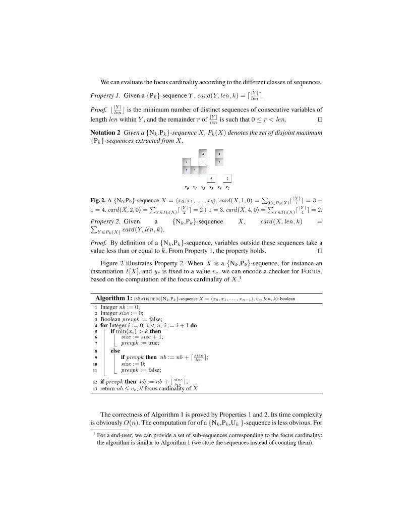
Fig. 2. A {N0,P0}-sequence X = �x0, x1, . . . , x5�. card(X, 1, 0) =�

Y ∈P0(X)�|Y |1� = 3 +

1 = 4. card(X, 2, 0) =�

Y ∈P0(X)�|Y |2� = 2+1 = 3. card(X, 4, 0) =

�Y ∈P0(X)�

|Y |4� = 2.

Property 2. Given a {Nk,Pk}-sequence X , card(X, len, k) =�Y ∈Pk(X) card(Y, len, k).

Proof. By definition of a {Nk,Pk}-sequence, variables outside these sequences take a

value less than or equal to k. From Property 1, the property holds. ��

Figure 2 illustrates Property 2. When X is a {Nk,Pk}-sequence, for instance an

instantiation I[X], and yc is fixed to a value vc, we can encode a checker for FOCUS,

based on the computation of the focus cardinality of X .1

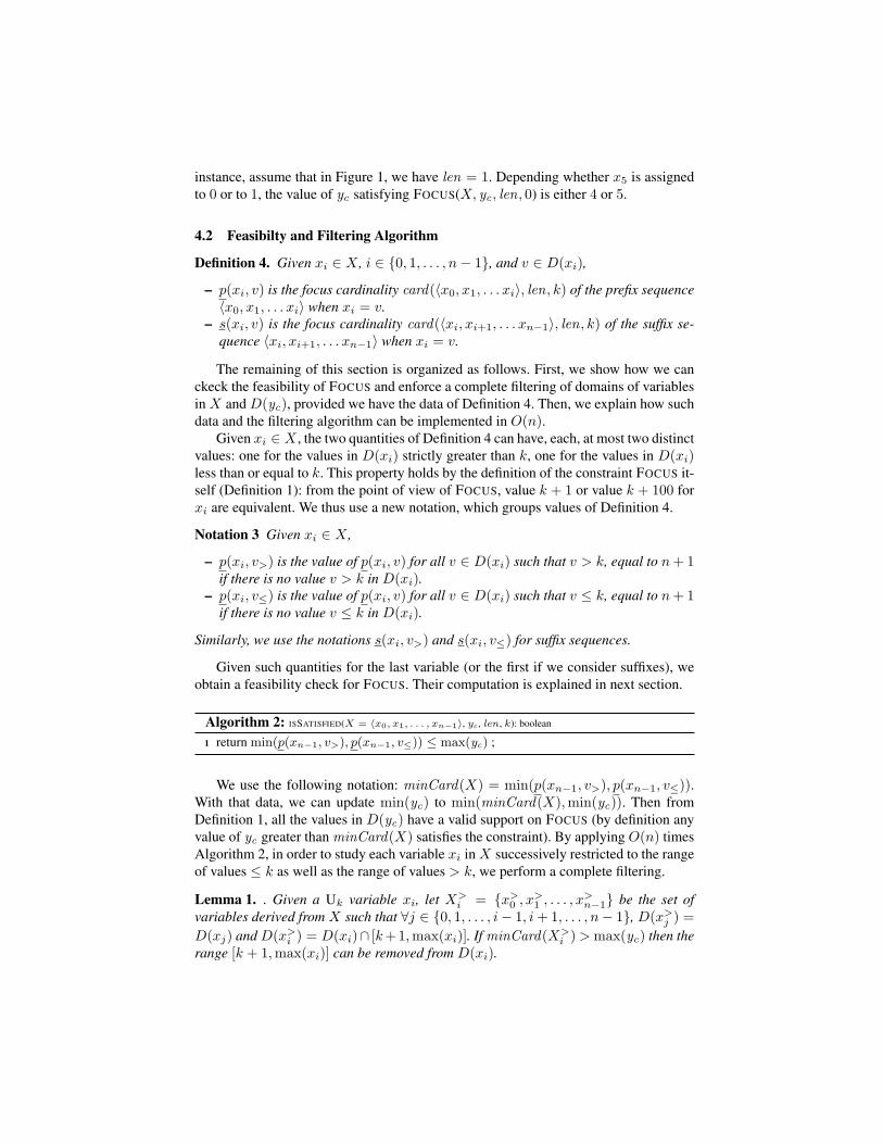
Algorithm 1: ISSATISFIED({Nk ,Pk}-sequence X = �x0, x1, . . . , xn−1�, vc, len , k): boolean

1 Integer nb := 0;2 Integer size := 0;3 Boolean prevpk := false;4 for Integer i := 0; i < n; i := i+ 1 do5 if min(xi) > k then6 size := size + 1;7 prevpk := true;

8 else9 if prevpk then nb := nb + � size

len�;

10 size := 0;11 prevpk := false;

12 if prevpk then nb := nb + � size

len�;

13 return nb ≤ vc; // focus cardinality of X

The correctness of Algorithm 1 is proved by Properties 1 and 2. Its time complexity

is obviously O(n). The computation for of a {Nk,Pk,Uk }-sequence is less obvious. For

1 For a end-user, we can provide a set of sub-sequences corresponding to the focus cardinality:

the algorithm is similar to Algorithm 1 (we store the sequences instead of counting them).

instance, assume that in Figure 1, we have len = 1. Depending whether x5 is assigned

to 0 or to 1, the value of yc satisfying FOCUS(X, yc , len, 0) is either 4 or 5.

4.2 Feasibilty and Filtering Algorithm

Definition 4. Given xi ∈ X , i ∈ {0, 1, . . . , n− 1}, and v ∈ D(xi),

– p(xi, v) is the focus cardinality card(�x0, x1, . . . xi�, len, k) of the prefix sequence

�x0, x1, . . . xi� when xi = v.

– s(xi, v) is the focus cardinality card(�xi, xi+1, . . . xn−1�, len, k) of the suffix se-

quence �xi, xi+1, . . . xn−1� when xi = v.

The remaining of this section is organized as follows. First, we show how we can

ckeck the feasibility of FOCUS and enforce a complete filtering of domains of variables

in X and D(yc), provided we have the data of Definition 4. Then, we explain how such

data and the filtering algorithm can be implemented in O(n).Given xi ∈ X , the two quantities of Definition 4 can have, each, at most two distinct

values: one for the values in D(xi) strictly greater than k, one for the values in D(xi)less than or equal to k. This property holds by the definition of the constraint FOCUS it-

self (Definition 1): from the point of view of FOCUS, value k + 1 or value k + 100 for

xi are equivalent. We thus use a new notation, which groups values of Definition 4.

Notation 3 Given xi ∈ X ,

– p(xi, v>) is the value of p(xi, v) for all v ∈ D(xi) such that v > k, equal to n+ 1if there is no value v > k in D(xi).

– p(xi, v≤) is the value of p(xi, v) for all v ∈ D(xi) such that v ≤ k, equal to n+ 1if there is no value v ≤ k in D(xi).

Similarly, we use the notations s(xi, v>) and s(xi, v≤) for suffix sequences.

Given such quantities for the last variable (or the first if we consider suffixes), we

obtain a feasibility check for FOCUS. Their computation is explained in next section.

Algorithm 2: ISSATISFIED(X = �x0, x1, . . . , xn−1�, yc , len , k): boolean

1 return min(p(xn−1, v>), p(xn−1, v≤)) ≤ max(yc) ;

We use the following notation: minCard(X) = min(p(xn−1, v>), p(xn−1, v≤)).With that data, we can update min(yc) to min(minCard(X),min(yc)). Then from

Definition 1, all the values in D(yc) have a valid support on FOCUS (by definition any

value of yc greater than minCard(X) satisfies the constraint). By applying O(n) times

Algorithm 2, in order to study each variable xi in X successively restricted to the range

of values ≤ k as well as the range of values > k, we perform a complete filtering.

Lemma 1. . Given a Uk variable xi, let X>i = {x>

0 , x>1 , . . . , x

>n−1} be the set of

variables derived from X such that ∀j ∈ {0, 1, . . . , i− 1, i+ 1, . . . , n− 1}, D(x>j ) =

D(xj) and D(x>i ) = D(xi)∩ [k+1,max(xi)]. If minCard(X>

i )>max(yc) then the

range [k + 1,max(xi)] can be removed from D(xi).

Lemma 2. Given a Uk variable xi, let X>i = {x>

0 , x>1 , . . . , x

>n−1} be the set of vari-

ables derived from X such that ∀j ∈ {0, 1, . . . , i−1, i+1, . . . , n−1}, D(x≤j ) = D(xj)

and D(x≤i ) = D(xi) ∩ [min(xi), k]. If minCard(X≤

i ) > max(yc) then the range

[k + 1,max(xi)] can be removed from D(xi).

Proof (Lemmas 1 and 2). Direct consequence of Definitions 1 and 3. ��

Given O(Φ) the time complexity of an algorithm computing minCard(X), we can

perform the complete filtering of variables in X ∪ {yc} in O(n × Φ), where n = |X|.We now show how to decrease the whole time complexity to O(n), both for computing

minCard(X) and shrink the domains of all the variables in X . Given xi ∈ X , the

idea is to compute p(xi, v>) from p(xi−1, v>) and p(xi−1, v≤). To do so, we have to

estimate the minimum length of a {Pk}-sequence containing xi, within an instantiation

of �x0, x1, . . . , xi� of focus cardinality p(xi, v>). We call this quantity plen(xi). Next

lemmas provide the values of p(xi, v>), p(xi−1, v≤) and plen(xi), from xi−1.

Lemma 3 (case of x0).

– If xi is a {Pk}-variable, p(x0, v≤) = n+ 1, p(x0, v>) = 1 and plen(x0) = 1.

– If xi is a {Nk}-variable, p(x0, v≤) = 0, p(x0, v>) = n+ 1 and plen(x0) = 0.

– If xi is a {Uk}-variable, p(x0, v≤) = 0, p(x0, v>) = 1 and plen(x0) = 1.

Proof. If x0 takes a value v > k then by Definition 4 p(x0, v>) = 1 and plen(x0) = 1.

Otherwise, there is no {Pk}-sequence containing x0 and plen(x0) = 0: We use the

convention p(x0, v>) = n+ 1 (an absurd value: the max. number of sequences in X is

n). If x0 belongs to a {Pk}-sequence then p(x0, v≤) = n+ 1. ��

Lemma 4 (computation of p(xi, v≤), 0 < i < n). If xi is a {Pk}-variable then

p(xi, v≤) = n+ 1. Otherwise, p(xi, v≤) = min(p(xi−1, v>), p(xi−1, v≤)).

Proof. If xi belongs to a {Pk}-sequence then xi does not take a value v ≤ k, thus

p(x0, v≤) = n + 1. If there exists some values less than or equal to k in D(xi),assigning one such value to xi leads to a number of {Pk}-sequences within the pre-

fix sequence �x0, x1, . . . , xi� which does not increase compared with the sequence

�x0, x1, . . . , xi−1�. Thus, p(xi, v≤) = min(p(xi−1, v>), p(xi−1, v≤)). ��

Lemma 5 (computation of p(xi, v>) and plen(xi), 0 < i < n). We have:

– If xi is a {Nk}-variable then p(xi, v>) = n+ 1 and plen(xi) = 0.

– Otherwise,

• If plen(xi−1) = len ∨ plen(xi−1) = 0 then

p(xi, v>) = min(p(xi−1, v>) + 1, p(xi−1, v≤) + 1) and plen(xi) = 1.

• Otherwise p(xi, v>) = min(p(xi−1, v>), p(xi−1, v≤) + 1) and:

∗ If p(xi−1, v>) ≤ p(xi−1, v≤) then plen(xi) = plen(xi−1) + 1.

∗ Else plen(xi) = 1.

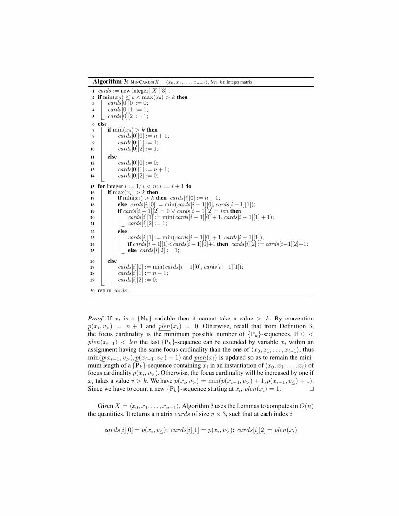
Algorithm 3: MINCARDS(X = �x0, x1, . . . , xn−1�, len, k): Integer matrix

1 cards := new Integer[|X|][3] ;2 if min(x0) ≤ k ∧ max(x0) > k then3 cards[0][0] := 0;4 cards[0][1] := 1;5 cards[0][2] := 1;

6 else7 if min(x0) > k then8 cards[0][0] := n+ 1;9 cards[0][1] := 1;

10 cards[0][2] := 1;

11 else12 cards[0][0] := 0;13 cards[0][1] := n+ 1;14 cards[0][2] := 0;

15 for Integer i := 1; i < n; i := i+ 1 do16 if max(xi) > k then17 if min(xi) > k then cards[i][0] := n+ 1;18 else cards[i][0] := min(cards[i− 1][0], cards[i− 1][1]);19 if cards[i− 1][2] = 0 ∨ cards[i− 1][2] = len then20 cards[i][1] := min(cards[i− 1][0] + 1, cards[i− 1][1] + 1);21 cards[i][2] := 1;

22 else23 cards[i][1] := min(cards[i− 1][0] + 1, cards[i− 1][1]);24 if cards[i− 1][1]<cards[i− 1][0]+1 then cards[i][2] := cards[i−1][2]+1;25 else cards[i][2] := 1;

26 else27 cards[i][0] := min(cards[i− 1][0], cards[i− 1][1]);28 cards[i][1] := n+ 1;29 cards[i][2] := 0;

30 return cards;

Proof. If xi is a {Nk}-variable then it cannot take a value > k. By convention

p(xi, v>) = n + 1 and plen(xi) = 0. Otherwise, recall that from Definition 3,

the focus cardinality is the minimum possible number of {Pk}-sequences. If 0 <plen(xi−1) < len the last {Pk}-sequence can be extended by variable xi within an

assignment having the same focus cardinality than the one of �x0, x1, . . . , xi−1�, thus

min(p(xi−1, v>), p(xi−1, v≤) + 1) and plen(xi) is updated so as to remain the mini-

mum length of a {Pk}-sequence containing xi in an instantiation of �x0, x1, . . . , xi� of

focus cardinality p(xi, v>). Otherwise, the focus cardinality will be increased by one if

xi takes a value v > k. We have p(xi, v>) = min(p(xi−1, v>) + 1, p(xi−1, v≤) + 1).Since we have to count a new {Pk}-sequence starting at xi, plen(xi) = 1. ��

Given X = �x0, x1, . . . , xn−1�, Algorithm 3 uses the Lemmas to computes in O(n)the quantities. It returns a matrix cards of size n× 3, such that at each index i:

cards[i][0] = p(xi, v≤); cards[i][1] = p(xi, v>); cards[i][2] = plen(xi)

We can then compute for each xi s(xi, v>), s(xi−1, v≤) and slen(xi) (the equiv-

alent of plen(xi) for suffixes), by using Lemmas 3, 4 and 5 with X sorted in the re-

verse order: �xn−1, xn−2, . . . , x0�. To estimate for each variable minCard(X≤i ) and

minCard(X>i ), we have to aggregate the quantities on prefixes and suffixes.

Property 3. minCard(X≤i ) = p(xi, v≤) + s(xi, v≤) and minCard(X>

i ) is equal to:

– p(xi, v>) + s(xi, v>)− 1 if and only if plen(xi) + slen(xi) −1 ≤ len .

– p(xi, v>) + s(xi, v>) otherwise.

Proof. Any pair of instantiations of focus cardinality respectively equal to p(xi, v≤)and s(xi, v≤) correspond to disjoint {Pk}-sequences (which do not contain xi). Thus

the quantities are independent and can be summed. With respect to minCard(X>i ), the

last current {Pk}-sequence taken into account in p(xi, v>) and s(xi, v>) contains xi.

Thus, their union (of length plen(xi) + slen(xi) −1) forms a unique {Pk}-sequence,

from which the maximum-length sub-sequence containing xi should not be counted

twice when it is not strictly larger than len . ��

Changing one value in an instantiation modifies its focus cardinality of at most one.

Property 4. Let I[X] = �v0, v1, . . . , vn−1� be an instantiation of focus cardinality

vc and xi ∈ X , and I �[X] = �v�0, v�1, . . . , v

�n−1� be the instantiation such that ∀j ∈

{0, 1, . . . , n − 1}, j �= i, vj = v�j and: (1) If vi > k then v�i ≤ k. (2) If vi ≤ k then

v�i > k. The focus cardinality v�c of I �[X] is such that |vc − v�c| ≤ 1.

Proof. Assume first that vi > k. xi belongs to a {Pk}-sequence p. Let s be the length

of this {Pk}-sequence within I[X]. We can split p into p1 = �xk, xk+1, . . . , xi−1�,p2 = �xi�, p3 = �xi+1, xi+1, . . . , xl� (p1 and/or p3 can be empty). Let q1, q3 and r1, r3be positive or null integers such that r1 < len, r3 < len and s = q1×len+r1+1+q3×len + r3. By construction, the maximum contribution of the variables in p to the focus

cardinality of I �[X] (that is, with xi ≤ k), is equal to q1+1 + q3+1=q1+ q3+2. With

respect to I[X], the contribution is then equal to q1 + q3 + � r1+r3+1len

�. The minimum

value of � r1+r3+1len

� is 1. In this case the property holds. The minimum contribution of

the variables in p to the focus cardinality of I �[X] is equal to q1 + q3. In this case, with

respect to I[X] the maximum value of � r1+r3+1len

� is � 1len

� = 1, the property holds.

The last intermediary case is when the contribution of the variables in p to the focus

cardinality of I �[X] is equal to q1 + q3 + 1. The minimum value of � r1+r3+1len

� is 1 and

its maximum is 2, the property holds. The reasoning for vi ≤ k is symmetrical. ��

From Property 4, we know that domains of variables in X can be pruned only once

yc is fixed since the variation coming from a single variable in X is at most one.

Algorithm 4 shrinks D(yc) as well as the domains of all variables in X in O(n). It

first calls Algorithm 3 to obtain minCard(X) from the values of min(p(xn−1, v>) and

p(xn−1, v≤)) and eventually shrink the domain of yc . Then, it computes the data for

suffixes, and uses Property 3 to reduce domains of variables in X according to max(yc).We present an implementation where the domains are not directly modified: X and ycare locally copied, and once the copies are filtered they are returned by the procedure.

The reason is that we will use this algorithm in an extension of FOCUS in Section 5).

To improve the readability, we assume that the solver raises automatically an exception

FAILEXCEPTION if a domain of one of these local copies becomes empty.

Algorithm 4: FILTER(X = �x0, x1, . . . , xn−1�, yc , len, k): Set of variables

1 cards := MINCARDS(X, len, k) ;2 Integer lb := min(cards[n− 1][0], cards[n− 1][1]);3 if min(yc) < lb then D(yc) := D(yc) \ [min(yc), lb[;4 if min(yc) = max(yc) then5 sdrac := MINCARDS(�xn−1, xn−2, . . . , x0�, len, k) ;6 for Integer i := 0; i < n; i := i+ 1 do7 if cards[i][0] + sdrac[n− 1− i][0] > max(yc) then8 D(xi) := D(xi)\ [min(xi), k];

9 Integer regret := 0;10 if cards[i][2] + sdrac[n− 1− i][2]− 1 ≤ len then regret := 1;11 if cards[i][1] + sdrac[n− 1− i][1]− regret > max(yc) then12 D(xi) := D(xi)\ ]k,max(xi)];

13 return X ∪ {yc};

Example 3. Consider FOCUS(X = �x0, x1, . . . , x4�, yc , len, 0) and D(yc) = {1, 2}.

(1) Assume len = 2 and D(x0)=D(x2)=D(x3)={1, 2}, D(x1) = {0} and D(x4)={0, 1, 2}. Line 3 of Algorithm 4 removes [1, 2[ from D(yc). Since the length of

the {Pk}-sequence �x2, x3� is equal to len , cards[4][1]=3 and cards[4][2]=1. sdrac

[5−1−4][1]=1 and sdrac[5−1−4][2]=1. regret=1 and thus 3+1−regret=3>max(yc),]0, 2] is removed from D(x4) (line 12). (2) Assume now len=3 and D(x0)=D(x2)=D(x4)={1, 2}, D(x1)={0} and D(x3)={0, 1, 2}. Line 3 of Algorithm 4 removes

[1, 2[ from D(yc). Since value 0 for x3 leads to a focus cardinality of 3 (cards[3][0] =2and sdrac[5−1−3][0]=1), strictlty greater than max(yc), �x2, x3, x4� must be a {Pk}-

sequence (of length 3 ≤ len). Algorithm 4 removes value 0 from D(x3) (line 8). �

5 Constraints Derived from FOCUS

Using a Variable for len Assume that, in Example 1 of Introduction, several com-

panies offer leases with different maximum duration. We aim at computing the best

possible configuration for each different offer, based on each maximum duration. To

deal with this case, we can extend FOCUS so as to define len as a variable, with a

discrete domain since the maximum durations of rentals are proper to each company.

Another use of this extension is the case where the end-user wishes to compare for the

same company several maximum package durations, enumerate several solutions, etc.

The filtering algorithm of this extension of FOCUS uses following principle: For

each value vl in D(len), we call FILTER(X, yc , vl, k) (Algorithm 4). If an exception

FAILEXCEPTION is raised, vl is removed from D(len). Otherwise, we store the result

of the filtering. At the end of the process, value v ∈ D(xi), xi ∈ X , is removed from its

domain if and only if it was removed by all the calls to FILTER(X, yc , vl, k) that did not

raised an exception. Algorithm 5 implements this principle. Since it calls Algorithm 4

for each value in D(len), it enforces GAC. Its time complexity is O(n× |D(len)|).

Harder constraint on yc In Definition 1, the number of sequences in S could be

constrained by an equality: |S| = vc. When the maximum value for the variable yc is

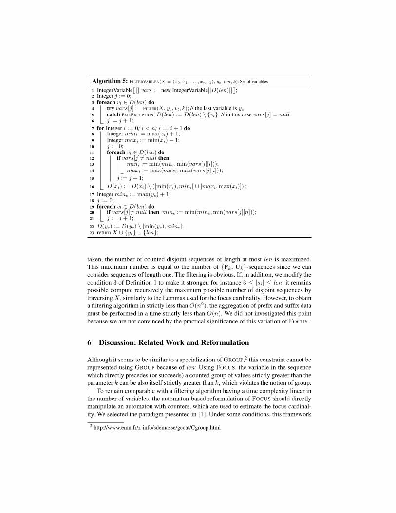
Algorithm 5: FILTERVARLEN(X = �x0, x1, . . . , xn−1�, yc , len, k): Set of variables

1 IntegerVariable[][] vars := new IntegerVariable[|D(len)|][];2 Integer j := 0;3 foreach vl ∈ D(len) do4 try vars[j] := FILTER(X, yc , vl, k); // the last variable is yc5 catch FAILEXCEPTION: D(len) := D(len) \ {vl}; // in this case vars[j] = null6 j := j + 1;

7 for Integer i := 0; i < n; i := i+ 1 do8 Integer mini := max(xi) + 1;9 Integer maxi := min(xi)− 1;

10 j := 0;11 foreach vl ∈ D(len) do12 if vars[j] �= null then13 mini := min(mini,min(vars[j][i]));14 maxi := max(maxi,max(vars[j][i]));

15 j := j + 1;

16 D(xi) := D(xi) \ ([min(xi),mini[ ∪ ]maxi,max(xi)]) ;

17 Integer minc := max(yc) + 1;18 j := 0;19 foreach vl ∈ D(len) do20 if vars[j] �= null then minc := min(minc,min(vars[j][n]));21 j := j + 1;

22 D(yc) := D(yc) \ [min(yc),minc[;23 return X ∪ {yc} ∪ {len};

taken, the number of counted disjoint sequences of length at most len is maximized.

This maximum number is equal to the number of {Pk, Uk}-sequences since we can

consider sequences of length one. The filtering is obvious. If, in addition, we modify the

condition 3 of Definition 1 to make it stronger, for instance 3 ≤ |si| ≤ len , it remains

possible compute recursively the maximum possible number of disjoint sequences by

traversing X , similarly to the Lemmas used for the focus cardinality. However, to obtain

a filtering algorithm in strictly less than O(n2), the aggregation of prefix and suffix data

must be performed in a time strictly less than O(n). We did not investigated this point

because we are not convinced by the practical significance of this variation of FOCUS.

6 Discussion: Related Work and Reformulation

Although it seems to be similar to a specialization of GROUP,2 this constraint cannot be

represented using GROUP because of len: Using FOCUS, the variable in the sequence

which directly precedes (or succeeds) a counted group of values strictly greater than the

parameter k can be also itself strictly greater than k, which violates the notion of group.

To remain comparable with a filtering algorithm having a time complexity linear in

the number of variables, the automaton-based reformulation of FOCUS should directly

manipulate an automaton with counters, which are used to estimate the focus cardinal-

ity. We selected the paradigm presented in [1]. Under some conditions, this framework

2 http://www.emn.fr/z-info/sdemasse/gccat/Cgroup.html

leads to a reformulation where a complete filtering is achieved, despite the counters.3

This paradigm is based on automata derived from constraint checkers. We propose an

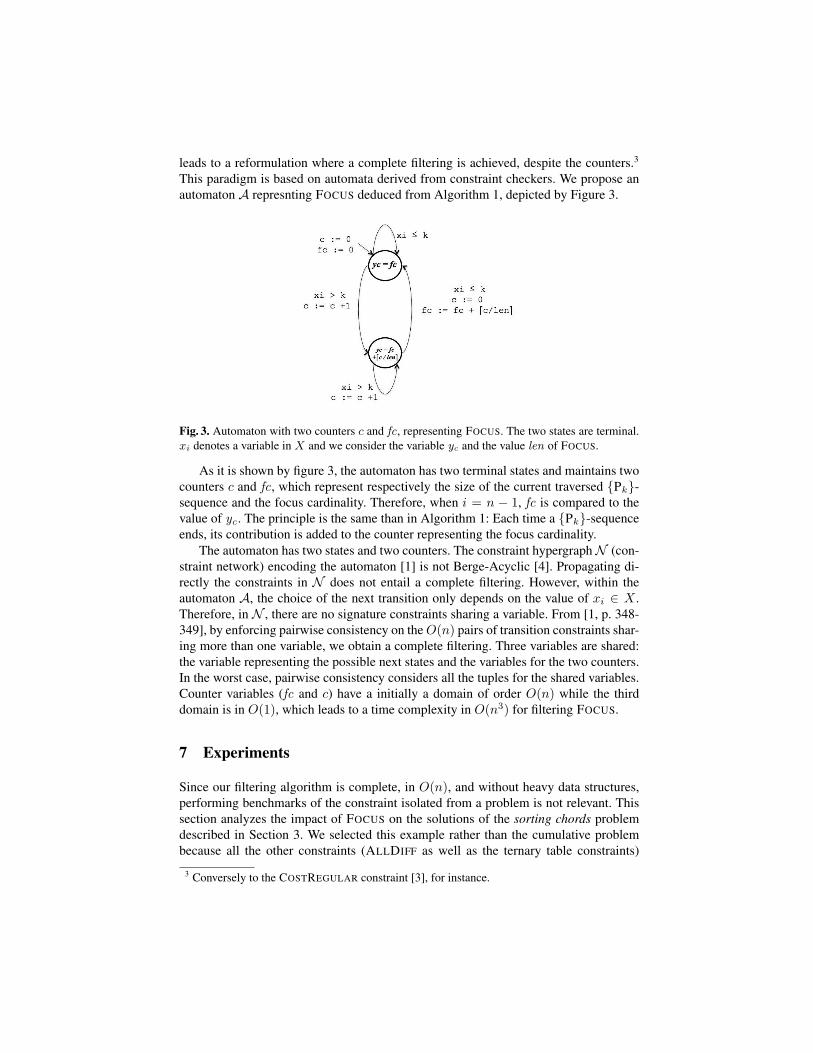
automaton A represnting FOCUS deduced from Algorithm 1, depicted by Figure 3.

Fig. 3. Automaton with two counters c and fc, representing FOCUS. The two states are terminal.

xi denotes a variable in X and we consider the variable yc and the value len of FOCUS.

As it is shown by figure 3, the automaton has two terminal states and maintains two

counters c and fc, which represent respectively the size of the current traversed {Pk}-

sequence and the focus cardinality. Therefore, when i = n − 1, fc is compared to the

value of yc . The principle is the same than in Algorithm 1: Each time a {Pk}-sequence

ends, its contribution is added to the counter representing the focus cardinality.

The automaton has two states and two counters. The constraint hypergraph N (con-

straint network) encoding the automaton [1] is not Berge-Acyclic [4]. Propagating di-

rectly the constraints in N does not entail a complete filtering. However, within the

automaton A, the choice of the next transition only depends on the value of xi ∈ X .

Therefore, in N , there are no signature constraints sharing a variable. From [1, p. 348-

349], by enforcing pairwise consistency on the O(n) pairs of transition constraints shar-

ing more than one variable, we obtain a complete filtering. Three variables are shared:

the variable representing the possible next states and the variables for the two counters.

In the worst case, pairwise consistency considers all the tuples for the shared variables.

Counter variables (fc and c) have a initially a domain of order O(n) while the third

domain is in O(1), which leads to a time complexity in O(n3) for filtering FOCUS.

7 Experiments

Since our filtering algorithm is complete, in O(n), and without heavy data structures,

performing benchmarks of the constraint isolated from a problem is not relevant. This

section analyzes the impact of FOCUS on the solutions of the sorting chords problem

described in Section 3. We selected this example rather than the cumulative problem

because all the other constraints (ALLDIFF as well as the ternary table constraints)

3 Conversely to the COSTREGULAR constraint [3], for instance.

can be provided with a complete filtering algorithm. With respect to the variable sum ,

we define it as the objective to minimize. Thus, instead of an equality we enforce

the constraint sum ≤�

cost i, which is also tractable. We use the solver Choco

(http://www.emn.fr/z-info/choco-solver/) with the default variable and value search

strategies (DomOverWDeg and MinValue), on a Mac OSX 2.2 Ghz Intel Core i7 with

8go of RAM memory. We are interested in two aspects:

1. Our constraint is used for refining an objective criterion and, from Property 4, we

know that domains of variables in X can be pruned only once yc is fixed. An

important question is the following: is our filtering algorithm significantly useful

during the search, compared with a simple checker?

2. Are the instances harder and/or the objective value of the variable sum widely

increased when we restrict the set of solutions by imposing FOCUS?

Pruning Efficacy In a first experiment, we run sets of 100 random instances of the

sorting chords problem, in order to compare the complete filtering of FOCUS with a

simple checker. For each set, the maximum value of yc is either 1 or 2, in order to

consider instances where FOCUS as a important influence. We compare the pruning ef-

ficacy of FOCUS with a light version of FOCUS, where the propagation is reduced to the

checker. Table 1 summarizes the results on 8 and 9 chords (respectively 17 and 19 vari-

ables in the problem). The instances are all satisfiable and optima were always proved.

With larger instances (≥ 10 chords), optimum cannot be proved in a reasonable num-

ber of backtracks using the checker. In the table, yc = max(yc), and len and k are the

parameters of FOCUS. nmax is the maximum possible number of changing notes be-

tween any two chords. Average values are given as integers. Table 1 shows clearly that,

even with a GAC filtering algorithm for ALLDIFF and for the ternary table constraints

COSTC(chi, chi+1, costi), we can only solve small instances without propagating FO-

CUS, some of them requiring more than one million backtracks. Conversely, the number

of backtracks for proving optimality is small and stable when Algorithm 4 is used for

propagating FOCUS. Using the filtering algorithm of FOCUS is mandatory.

Impact on the Objective Value We run sets of 100 random instances of the sort-

ing chords problem, in order to compare problems involving FOCUS with the same

problems where FOCUS is removed from the model. The goal of this experiment is to

determine whether the optimum objective value increases widely or not, as well as the

time and backtracks required to obtain such optimum values. Table 2 summarizes the

results with a number of chords varying from 6 to 20 (13 to 51 variables in the problem).

The instances are all satisfiable and optima were always found and proved. In each set,

we count the number of instances with distinct objective values. For sake of space, we

present the results for k = 0 and len = 4. Similar results were found for closed values

of k and len . Despite the instances with FOCUS are more constrained with respect to

the variables involved in the objective, Table 2 does not reveals any significant differ-

ence, both with respect to the number of backtracks (and solving time) and the optimum

objective value. We finally have differences in objective values at most equal to 2.

To complete our evaluation, we search for the first solution of larger problems, in

order to compare the scale of size that can be reached with and without using FOCUS.

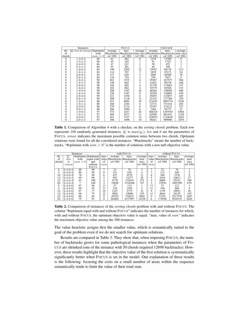
Instances FOCUS CHECKER

nb. yc -len-k-nmax #optimum average max. average average max. averageof with #backtracks #backtracks time (ms) #backtracks #backtracks time (ms)

chords sum > 0 (of 100) (of 100) (of 100) (of 100) (of 100) (of 100)8 1-4-0-3 66 61 462 11 1518 15300 178 1-4-1-3 66 45 342 1 91 1724 28 2-4-0-3 66 47 247 1 58 455 18 2-4-1-3 66 45 301 1 44 349 18 1-6-0-4 84 198 2205 12 15952 86778 2138 1-6-1-4 84 114 767 3 1819 45171 248 2-6-0-4 84 127 620 3 2069 64509 288 2-6-1-4 84 118 724 3 250 7027 48 1-8-0-5 98 261 1533 6 39307 167575 5668 1-8-1-5 98 148 662 3 11821 94738 1688 2-8-0-5 98 164 803 4 21739 173063 3178 1-8-0-5 98 183 882 4 10779 92560 1538 1-8-0-6 99 290 1187 18 46564 130058 6908 1-8-1-6 99 238 1167 11 29256 134882 4388 2-8-0-6 99 221 1458 6 29455 123857 4458 2-8-1-6 99 209 1118 13 21332 117768 3299 1-9-0-4 88 415 4003 18 214341 1095734 32449 1-9-1-4 88 268 2184 6 12731 751414 2039 2-9-0-4 88 270 2714 6 22107 374121 3379 2-9-1-4 88 266 3499 6 1364 92773 239 1-9-0-5 97 574 2437 26 360324 1355934 65849 1-9-1-5 97 404 1677 11 62956 881441 11509 2-9-0-5 97 451 3327 12 228072 1124630 42639 2-9-1-5 97 386 1698 10 58421 989900 1079

Table 1. Comparison of Algorithm 4 with a checker, on the sorting chords problem. Each row

represents 100 randomly generated instances. yc is max(yc), len and k are the parameters of

FOCUS. nmax indicates the maximum possible common notes between two chords. Optimum

solutions were found for all the considered instances. “#backtracks” means the number of back-

tracks, “#optimum with sum > 0” is the number of solutions with a non null objective value.

Instances with FOCUS without FOCUS

nb. yc #optimum #optimum max. average max. average max. average max. averageof -len with equal with value #backtracks #backtracks time value #backtracks #backtracks time

chords -k sum > 0 and of (of 100) (of 100) (ms) of (of 100) (of 100) (ms)-nmax without sum (of 100) sum (of 100)

FOCUS

6 2-4-0-4 88 99 7 23 76 3 7 22 76 18 2-4-0-4 84 95 8 131 618 4 7 115 449 310 2-4-0-4 78 98 6 457 4579 11 6 360 3376 912 2-4-0-4 69 98 5 952 12277 28 5 1010 10812 2716 2-4-0-4 43 100 4 4778 132019 153 4 6069 95531 18920 2-4-0-4 7 100 3 15650 1316296 747 3 15970 1095399 6796 2-4-0-6 97 96 13 37 113 1 13 37 121 18 2-4-0-6 99 93 11 218 1305 5 11 198 860 410 2-4-0-6 97 77 10 1247 5775 32 9 1159 10921 2612 2-4-0-6 96 75 12 5092 34098 155 11 4844 54155 14516 2-4-0-6 88 84 9 45935 724815 2002 9 73251 2517570 340720 2-4-0-6 79 91 8 264881 4157997 14236 6 174956 2918335 8284

Table 2. Comparison of instances of the sorting chords problem with and without FOCUS. The

column “#optimum equal with and without FOCUS” indicates the number of instances for which,

with and without FOCUS, the optimum objective value is equal. “max. value of sum” indicates

the maximum objective value among the 100 instances.

The value heuristic assigns first the smaller value, which is semantically suited to the

goal of the problem even if we do not search for optimum solutions.

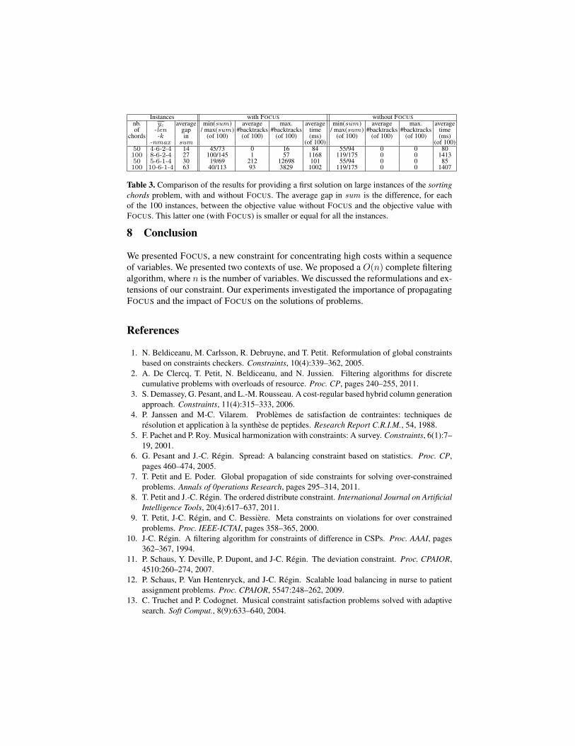
Results are compared in Table 3. They show that, when imposing FOCUS, the num-

ber of backtracks grows for some pathological instances when the parameters of FO-

CUS are shrinked (one of the instance with 50 chords required 12698 backtracks). How-

ever, these results highlight that the objective value of the first solution is systematically

significantly better when FOCUS is set in the model. One explanation of these results

is the following: focusing the costs on a small number of areas within the sequence

semantically tends to limit the value of their total sum.

Instances with FOCUS without FOCUS

nb. yc average min(sum) average max. average min(sum) average max. averageof -len gap / max(sum) #backtracks #backtracks time / max(sum) #backtracks #backtracks time

chords -k in (of 100) (of 100) (of 100) (ms) (of 100) (of 100) (of 100) (ms)-nmax sum (of 100) (of 100)

50 4-6-2-4 14 45/73 0 16 84 55/94 0 0 80100 8-6-2-4 27 100/145 1 57 1168 119/175 0 0 141350 5-6-1-4 30 19/69 212 12698 101 55/94 0 0 85100 10-6-1-4 63 40/113 93 3829 1002 119/175 0 0 1407

Table 3. Comparison of the results for providing a first solution on large instances of the sorting

chords problem, with and without FOCUS. The average gap in sum is the difference, for each

of the 100 instances, between the objective value without FOCUS and the objective value with

FOCUS. This latter one (with FOCUS) is smaller or equal for all the instances.

8 Conclusion

We presented FOCUS, a new constraint for concentrating high costs within a sequence

of variables. We presented two contexts of use. We proposed a O(n) complete filtering

algorithm, where n is the number of variables. We discussed the reformulations and ex-

tensions of our constraint. Our experiments investigated the importance of propagating

FOCUS and the impact of FOCUS on the solutions of problems.

References

1. N. Beldiceanu, M. Carlsson, R. Debruyne, and T. Petit. Reformulation of global constraints

based on constraints checkers. Constraints, 10(4):339–362, 2005.

2. A. De Clercq, T. Petit, N. Beldiceanu, and N. Jussien. Filtering algorithms for discrete

cumulative problems with overloads of resource. Proc. CP, pages 240–255, 2011.

3. S. Demassey, G. Pesant, and L.-M. Rousseau. A cost-regular based hybrid column generation

approach. Constraints, 11(4):315–333, 2006.

4. P. Janssen and M-C. Vilarem. Problemes de satisfaction de contraintes: techniques de

resolution et application a la synthese de peptides. Research Report C.R.I.M., 54, 1988.

5. F. Pachet and P. Roy. Musical harmonization with constraints: A survey. Constraints, 6(1):7–

19, 2001.

6. G. Pesant and J.-C. Regin. Spread: A balancing constraint based on statistics. Proc. CP,

pages 460–474, 2005.

7. T. Petit and E. Poder. Global propagation of side constraints for solving over-constrained

problems. Annals of 0perations Research, pages 295–314, 2011.

8. T. Petit and J.-C. Regin. The ordered distribute constraint. International Journal on Artificial

Intelligence Tools, 20(4):617–637, 2011.

9. T. Petit, J-C. Regin, and C. Bessiere. Meta constraints on violations for over constrained

problems. Proc. IEEE-ICTAI, pages 358–365, 2000.

10. J-C. Regin. A filtering algorithm for constraints of difference in CSPs. Proc. AAAI, pages

362–367, 1994.

11. P. Schaus, Y. Deville, P. Dupont, and J-C. Regin. The deviation constraint. Proc. CPAIOR,

4510:260–274, 2007.

12. P. Schaus, P. Van Hentenryck, and J-C. Regin. Scalable load balancing in nurse to patient

assignment problems. Proc. CPAIOR, 5547:248–262, 2009.

13. C. Truchet and P. Codognet. Musical constraint satisfaction problems solved with adaptive

search. Soft Comput., 8(9):633–640, 2004.