
Constraint Integer Programming - OPUS 4 · Abstract This thesis introduces the novel paradigm of...
426
Constraint Integer Programming vorgelegt von Dipl.-Math. Dipl.-Inf. Tobias Achterberg Berlin der Fakultät II – Mathematik und Naturwissenschaften der Technischen Universität Berlin zur Erlangung des akademischen Grades Doktor der Naturwissenschaften – Dr. rer. nat. – genehmigte Dissertation Berichter: Prof. Dr. Dr. h.c. Martin Grötschel Technische Universität Berlin Prof. Dr. Robert E. Bixby Rice University, Houston, USA Tag der wissenschaftlichen Aussprache: 12. Juli 2007 Berlin 2007 D 83 genehmigte Fassung: 15. Mai 2007 überarbeitete Fassung: 10. Dezember 2008
Transcript of Constraint Integer Programming - OPUS 4 · Abstract This thesis introduces the novel paradigm of...
Constraint Integer Programming
vorgelegt vonDipl.-Math. Dipl.-Inf. Tobias Achterberg
Berlin
der Fakultät II – Mathematik und Naturwissenschaftender Technischen Universität Berlin
zur Erlangung des akademischen Grades
Doktor der Naturwissenschaften– Dr. rer. nat. –
genehmigte Dissertation
Berichter: Prof. Dr. Dr. h.c. Martin GrötschelTechnische Universität Berlin
Prof. Dr. Robert E. BixbyRice University, Houston, USA
Tag der wissenschaftlichen Aussprache: 12. Juli 2007
Berlin 2007D 83
genehmigte Fassung: 15. Mai 2007
überarbeitete Fassung: 10. Dezember 2008


Für Julia


Zusammenfassung
Diese Arbeit stellt einen integrierten Ansatz aus Constraint Programming (CP) undGemischt-Ganzzahliger Programmierung (Mixed Integer Programming, MIP) vor,den wir Constraint Integer Programming (CIP) nennen. Sowohl Modellierungs- alsauch Lösungstechniken beider Felder fließen in den neuen integrierten Ansatz ein,um die unterschiedlichen Stärken der beiden Gebiete zu kombinieren. Als weite-ren Beitrag stellen wir der wissenschaftlichen Gemeinschaft die Software SCIP zurVerfügung, die ein Framework für Constraint Integer Programming darstellt undzusätzlich Techniken des SAT-Lösens beinhaltet. SCIP ist im Source Code für aka-demische und nicht-kommerzielle Zwecke frei erhältlich.
Unser Ansatz des Constraint Integer Programming ist eine Verallgemeinerungvon MIP, die zusätzlich die Verwendung beliebiger Constraints erlaubt, solange sichdiese durch lineare Bedingungen ausdrücken lassen falls alle ganzzahligen Variablenauf feste Werte eingestellt sind. Die Constraints werden von einer beliebigen Kom-bination aus CP- und MIP-Techniken behandelt. Dies beinhaltet insbesondere dieDomain Propagation, die Relaxierung der Constraints durch lineare Ungleichungen,sowie die Verstärkung der Relaxierung durch dynamisch generierte Schnittebenen.
Die derzeitige Version von SCIP enthält alle Komponenten, die für das effizienteLösen von Gemischt-Ganzzahligen Programmen benötigt werden. Die vorliegendeArbeit liefert eine ausführliche Beschreibung dieser Komponenten und bewertet ver-schiedene Varianten in Hinblick auf ihren Einfluß auf das Gesamt-Lösungsverhaltenanhand von aufwendigen praktischen Experimenten. Dabei wird besonders auf diealgorithmischen Aspekte eingegangen.
Der zweite Hauptteil der Arbeit befasst sich mit der Chip-Design-Verifikation,die ein wichtiges Thema innerhalb des Fachgebiets der Electronic Design Automa-tion darstellt. Chip-Hersteller müssen sicherstellen, dass der logische Entwurf einerSchaltung der gegebenen Spezifikation entspricht. Andernfalls würde der Chip feh-lerhaftes Verhalten aufweisen, dass zu Fehlfunktionen innerhalb des Gerätes führenkann, in dem der Chip verwendet wird. Ein wichtiges Teilproblem in diesem Feldist das Eigenschafts-Verifikations-Problem, bei dem geprüft wird, ob der gegebeneSchaltkreisentwurf eine gewünschte Eigenschaft aufweist. Wir zeigen, wie dieses Pro-blem als Constraint Integer Program modelliert werden kann und geben eine Reihevon problemspezifischen Algorithmen an, die die Struktur der einzelnen Constraintsund der Gesamtschaltung ausnutzen. Testrechnungen auf Industrie-Beispielen ver-gleichen unseren Ansatz mit den bisher verwendeten SAT-Techniken und belegenden Erfolg unserer Methode.
v

Abstract
This thesis introduces the novel paradigm of constraint integer programming (CIP),which integrates constraint programming (CP) and mixed integer programming (MIP)modeling and solving techniques. It is supplemented by the software SCIP, whichis a solver and framework for constraint integer programming that also featuresSAT solving techniques. SCIP is freely available in source code for academic andnon-commercial purposes.
Our constraint integer programming approach is a generalization of MIP thatallows for the inclusion of arbitrary constraints, as long as they turn into linearconstraints on the continuous variables after all integer variables have been fixed.The constraints, may they be linear or more complex, are treated by any combinationof CP and MIP techniques: the propagation of the domains by constraint specificalgorithms, the generation of a linear relaxation and its solving by LP methods, andthe strengthening of the LP by cutting plane separation.
The current version of SCIP comes with all of the necessary components tosolve mixed integer programs. In the thesis, we cover most of these ingredientsand present extensive computational results to compare different variants for theindividual building blocks of a MIP solver. We focus on the algorithms and theirimpact on the overall performance of the solver.
In addition to mixed integer programming, the thesis deals with chip designverification, which is an important topic of electronic design automation. Chipmanufacturers have to make sure that the logic design of a circuit conforms to thespecification of the chip. Otherwise, the chip would show an erroneous behavior thatmay cause failures in the device where it is employed. An important subproblem ofchip design verification is the property checking problem, which is to verify whethera circuit satisfies a specified property. We show how this problem can be modeledas constraint integer program and provide a number of problem-specific algorithmsthat exploit the structure of the individual constraints and the circuit as a whole.Another set of extensive computational benchmarks compares our CIP approachto the current state-of-the-art SAT methodology and documents the success of ourmethod.
vii

Acknowledgements
Working at the Zuse Institute Berlin was a great experience for me, and thanks tothe very flexible people in the administrations and management levels of ZIB andmy new employer ILOG, this experience continues. It is a pleasure to be surroundedby lots of nice colleagues, even though some of them have the nasty habit to comeinto my office (without being formally invited!) with the only purpose of wastingmy time by asking strange questions about SCIP and Cplex. And eating a pieceof sponsored cake from time to time while discussing much more interesting topicsthan optimization or mathematical programming is always a valuable distraction.Thank you, Marc!
Work on this thesis actually began already in 2000 with the work on my computerscience master’s thesis. This was about applying neural networks to learn goodbranching strategies for MIP solvers. Research on such a topic is only possible ifyou have the source code of a state-of-the-art MIP solver. Fortunately, the formerZIB member Alexander Martin made his solver SIP available to me, such that I wasrelieved from inventing the wheel a second time. With the help of Thorsten Koch,I learned a lot by analyzing his algorithms.
Since I studied both, mathematics and computer science, I always looked for atopic that combines the two fields. In 2002, it came to my mind that the integrationof integer programming and constraint programming would be a perfect candidatein this regard. Unfortunately, such an integration was way beyond the scope ofSIP, such that I had to start from scratch at the end of 2002 with a quickly growingcode that I called SCIP in order to emphasize its relation to SIP. At this point,I have to thank my advisor Martin Grötschel for his patience and for the freedomhe offered me to do whatever I liked. For almost two years, I did not publish asingle paper! Instead, I was sitting in my office, hacking the whole day on my codein order to get a basis on which I can conduct the actual research. And then, themiracle occurred, again thanks to Martin Grötschel: his connections to the group ofWolfram Büttner at Infineon (which later became the spin-off company OneSpinSolutions) resulted in the perfect project at the perfect moment: solving the chipdesign verification problem, an ideal candidate to tackle with constraint integerprogramming methods.
During the two-year period of the project, which was called Valse-XT, I learneda lot about the logic design of chips and how its correctness can be verified. I thankRaik Brinkmann for all his support. Having him as the direct contact person of theindustry partner made “my” project considerably different from most of the otherprojects we had at ZIB: I obtained lots of test and benchmark data, and I receivedthe data early enough to be useful within the duration of the project.
Another interesting person I learned to know within the project is Yakov Novikov.He is a brilliant SAT researcher from Minsk who is now working for OneSpin Solu-tions in Munich. Because the Berlin administration is a little more “flexible” thanthe one of Bavaria, he came to Berlin in order to deal with all the bureaucratic affairsregarding his entry to Germany. We first met when I picked him up at a subwaystation after he arrived with the train at Berlin-Ostbahnhof. At the Ostbahnhof,he was mugged by a gang of Russians. They thought that he is a “typical” Eastern
ix
x Acknowledgements
European who carries a lot of cash in order to buy a car in Germany. Fortunately,by showing some of his papers he could convince them that he is only a poor re-searcher who does not have any money. After telling me this story, he explained tome the key concepts in SAT solving during the remaining 10 minutes in the subwaytrain: conflict analysis and the two watched literals scheme for fast Boolean con-straint propagation. I was very excited and started with the integration of the twowatched literals scheme into the set covering constraint handler a few days later.The generalization of conflict analysis to mixed integer programming followed afterthree weeks. As conflict analysis turned out to be a key ingredient for solving thechip verification problem with constraint integer programming, I am very thankfulto Yakov for pointing me into this direction.
I thought after having implemented more than 250 000 lines of C code for SCIPand the chip verification solver, the writing of the thesis would be a piece of cake.What a mistake! The time passed by, and suddenly I exceeded my self-imposed dead-line (to be finished before my 30th birthday) without having even started to writemy thesis. Of course, SCIP improved considerably during that time, which is alsothe contribution of my great students Kati Wolter and Timo Berthold. Additionally,the public visibility of SCIP increased dramatically, thanks to Hans Mittelmann’sbenchmarking website. Nevertheless, it needed Thorsten Koch to convince me thatstarting to write things down is more important than to improve the performanceof SCIP by another 10 %. I am very thankful for this advice!
Furthermore, I am very grateful to all the proof-readers of my thesis, which areTimo Berthold, Stefan Heinz, Thorsten Koch, and Marc Pfetsch from ZIB, MarkusWedler from TU Kaiserslautern, and Lloyd Clarke and Zonghao Gu from ILOG. Allof you helped me to improve the thesis quite a bit. Most of all, I would like to thankMarc Pfetsch, who actually read (and commented on) around 75 % of the thesis.I also thank Kathleen Callaway (ILOG) for her willingness to review the grammarand punctuation, but unfortunately she became sick and could not make it in time.Therefore, the reader has to live with my language deficiencies.
Finally, I thank my ZIB colleagues Andreas Eisenblätter, Stefan Heinz, MarikaNeumann, Sebastian Orlowski, Christian Raack, Thomas Schlechte, and Steffen Wei-der, who are the ones working on machines that are identical to mine, and whoallowed me to spend their spare CPU cycles on my benchmark runs.
Am allermeisten aber danke ich Dir, Julia. Du hast mir die ganze Zeit überden Rücken freigehalten und es insbesondere in den letzten vier Monaten ertragen,dass ich fast jeden Tag erst nach Mitternacht nach Hause gekommen bin und zumTeil auch die Wochenenden am ZIB verbracht habe. Ich bedaure es sehr, dass ichDich und die Kinder in dieser Zeit kaum zu Gesicht bekommen habe. Insbesonderesind die ersten sechs Lebensmonate von Mieke ziemlich schnell an mir vorüberge-zogen. Ab jetzt werde ich aber zu einem geregelten Familienleben zurückfinden.Ich liebe Dich!
Tobias AchterbergBerlin, May 2007
Contents
Introduction 1
I Concepts 7
1 Basic Definitions 91.1 Constraint Programs . . . . . . . . . . . . . . . . . . . . . . . . . . 91.2 Satisfiability Problems . . . . . . . . . . . . . . . . . . . . . . . . . 101.3 Mixed Integer Programs . . . . . . . . . . . . . . . . . . . . . . . . 111.4 Constraint Integer Programs . . . . . . . . . . . . . . . . . . . . . . 13
2 Algorithms 152.1 Branch and Bound . . . . . . . . . . . . . . . . . . . . . . . . . . . 152.2 Cutting Planes . . . . . . . . . . . . . . . . . . . . . . . . . . . . . . 182.3 Domain Propagation . . . . . . . . . . . . . . . . . . . . . . . . . . 19
3 SCIP as a CIP Framework 233.1 Basic Concepts of SCIP . . . . . . . . . . . . . . . . . . . . . . . . . 233.2 Algorithmic Design . . . . . . . . . . . . . . . . . . . . . . . . . . . 293.3 Infrastructure . . . . . . . . . . . . . . . . . . . . . . . . . . . . . . 37
II Mixed Integer Programming 57
4 Introduction 59
5 Branching 615.1 Most Infeasible Branching . . . . . . . . . . . . . . . . . . . . . . . 625.2 Least Infeasible Branching . . . . . . . . . . . . . . . . . . . . . . . 625.3 Pseudocost Branching . . . . . . . . . . . . . . . . . . . . . . . . . . 635.4 Strong Branching . . . . . . . . . . . . . . . . . . . . . . . . . . . . 635.5 Hybrid Strong/Pseudocost Branching . . . . . . . . . . . . . . . . . 645.6 Pseudocost Branching with
Strong Branching Initialization . . . . . . . . . . . . . . . . . . . . . 655.7 Reliability Branching . . . . . . . . . . . . . . . . . . . . . . . . . . 655.8 Inference Branching . . . . . . . . . . . . . . . . . . . . . . . . . . . 665.9 Hybrid Reliability/Inference Branching . . . . . . . . . . . . . . . . 675.10 Branching Rule Classification . . . . . . . . . . . . . . . . . . . . . . 685.11 Computational Results . . . . . . . . . . . . . . . . . . . . . . . . . 69
6 Node Selection 736.1 Depth First Search . . . . . . . . . . . . . . . . . . . . . . . . . . . 736.2 Best First Search . . . . . . . . . . . . . . . . . . . . . . . . . . . . 746.3 Best First Search with Plunging . . . . . . . . . . . . . . . . . . . . 756.4 Best Estimate Search . . . . . . . . . . . . . . . . . . . . . . . . . . 76
xi
xii Contents
6.5 Best Estimate Search with Plunging . . . . . . . . . . . . . . . . . . 776.6 Interleaved Best Estimate/Best First Search . . . . . . . . . . . . . 776.7 Hybrid Best Estimate/Best First Search . . . . . . . . . . . . . . . 786.8 Computational Results . . . . . . . . . . . . . . . . . . . . . . . . . 78
7 Domain Propagation 837.1 Linear Constraints . . . . . . . . . . . . . . . . . . . . . . . . . . . . 837.2 Knapsack Constraints . . . . . . . . . . . . . . . . . . . . . . . . . . 89
7.3 Set Partitioning and Set Packing Constraints . . . . . . . . . . . . . 917.4 Set Covering Constraints . . . . . . . . . . . . . . . . . . . . . . . . 937.5 Variable Bound Constraints . . . . . . . . . . . . . . . . . . . . . . 957.6 Objective Propagation . . . . . . . . . . . . . . . . . . . . . . . . . 967.7 Root Reduced Cost Strengthening . . . . . . . . . . . . . . . . . . . 987.8 Computational Results . . . . . . . . . . . . . . . . . . . . . . . . . 99
8 Cut Separation 1018.1 Knapsack Cover Cuts . . . . . . . . . . . . . . . . . . . . . . . . . . 1018.2 Mixed Integer Rounding Cuts . . . . . . . . . . . . . . . . . . . . . 1048.3 Gomory Mixed Integer Cuts . . . . . . . . . . . . . . . . . . . . . . 105
8.4 Strong Chvátal-Gomory Cuts . . . . . . . . . . . . . . . . . . . . . 1078.5 Flow Cover Cuts . . . . . . . . . . . . . . . . . . . . . . . . . . . . . 1088.6 Implied Bound Cuts . . . . . . . . . . . . . . . . . . . . . . . . . . . 1098.7 Clique Cuts . . . . . . . . . . . . . . . . . . . . . . . . . . . . . . . 1098.8 Reduced Cost Strengthening . . . . . . . . . . . . . . . . . . . . . . 1108.9 Cut Selection . . . . . . . . . . . . . . . . . . . . . . . . . . . . . . . 111
8.10 Computational Results . . . . . . . . . . . . . . . . . . . . . . . . . 111
9 Primal Heuristics 1179.1 Rounding Heuristics . . . . . . . . . . . . . . . . . . . . . . . . . . . 1189.2 Diving Heuristics . . . . . . . . . . . . . . . . . . . . . . . . . . . . 120
9.3 Objective Diving Heuristics . . . . . . . . . . . . . . . . . . . . . . . 1239.4 Improvement Heuristics . . . . . . . . . . . . . . . . . . . . . . . . . 1259.5 Computational Results . . . . . . . . . . . . . . . . . . . . . . . . . 127
10 Presolving 13310.1 Linear Constraints . . . . . . . . . . . . . . . . . . . . . . . . . . . . 13310.2 Knapsack Constraints . . . . . . . . . . . . . . . . . . . . . . . . . . 14610.3 Set Partitioning, Set Packing, and Set Covering Constraints . . . . 15110.4 Variable Bound Constraints . . . . . . . . . . . . . . . . . . . . . . 15310.5 Integer to Binary Conversion . . . . . . . . . . . . . . . . . . . . . . 154
10.6 Probing . . . . . . . . . . . . . . . . . . . . . . . . . . . . . . . . . . 15410.7 Implication Graph Analysis . . . . . . . . . . . . . . . . . . . . . . . 15710.8 Dual Fixing . . . . . . . . . . . . . . . . . . . . . . . . . . . . . . . 15810.9 Restarts . . . . . . . . . . . . . . . . . . . . . . . . . . . . . . . . . 16010.10 Computational Results . . . . . . . . . . . . . . . . . . . . . . . . . 161
11 Conflict Analysis 16511.1 Conflict Analysis in SAT Solving . . . . . . . . . . . . . . . . . . . . 16611.2 Conflict Analysis in MIP . . . . . . . . . . . . . . . . . . . . . . . . 17011.3 Computational Results . . . . . . . . . . . . . . . . . . . . . . . . . 178
Contents xiii
III Chip Design Verification 183
12 Introduction 185
13 Formal Problem Definition 18913.1 Constraint Integer Programming Model . . . . . . . . . . . . . . . . 18913.2 Function Graph . . . . . . . . . . . . . . . . . . . . . . . . . . . . . 192
14 Operators in Detail 19514.1 Bit and Word Partitioning . . . . . . . . . . . . . . . . . . . . . . . 19614.2 Unary Minus . . . . . . . . . . . . . . . . . . . . . . . . . . . . . . . 20414.3 Addition . . . . . . . . . . . . . . . . . . . . . . . . . . . . . . . . . 20414.4 Subtraction . . . . . . . . . . . . . . . . . . . . . . . . . . . . . . . . 21014.5 Multiplication . . . . . . . . . . . . . . . . . . . . . . . . . . . . . . 21114.6 Bitwise Negation . . . . . . . . . . . . . . . . . . . . . . . . . . . . . 22814.7 Bitwise And . . . . . . . . . . . . . . . . . . . . . . . . . . . . . . . 22814.8 Bitwise Or . . . . . . . . . . . . . . . . . . . . . . . . . . . . . . . . 23114.9 Bitwise Xor . . . . . . . . . . . . . . . . . . . . . . . . . . . . . . . 23114.10 Unary And . . . . . . . . . . . . . . . . . . . . . . . . . . . . . . . . 23414.11 Unary Or . . . . . . . . . . . . . . . . . . . . . . . . . . . . . . . . . 23714.12 Unary Xor . . . . . . . . . . . . . . . . . . . . . . . . . . . . . . . . 23714.13 Equality . . . . . . . . . . . . . . . . . . . . . . . . . . . . . . . . . 24114.14 Less-Than . . . . . . . . . . . . . . . . . . . . . . . . . . . . . . . . 24614.15 If-Then-Else . . . . . . . . . . . . . . . . . . . . . . . . . . . . . . . 25114.16 Zero Extension . . . . . . . . . . . . . . . . . . . . . . . . . . . . . . 25614.17 Sign Extension . . . . . . . . . . . . . . . . . . . . . . . . . . . . . . 25714.18 Concatenation . . . . . . . . . . . . . . . . . . . . . . . . . . . . . . 25714.19 Shift Left . . . . . . . . . . . . . . . . . . . . . . . . . . . . . . . . . 25714.20 Shift Right . . . . . . . . . . . . . . . . . . . . . . . . . . . . . . . . 26414.21 Slicing . . . . . . . . . . . . . . . . . . . . . . . . . . . . . . . . . . 26414.22 Multiplex Read . . . . . . . . . . . . . . . . . . . . . . . . . . . . . 26714.23 Multiplex Write . . . . . . . . . . . . . . . . . . . . . . . . . . . . . 272
15 Presolving 27915.1 Term Algebra Preprocessing . . . . . . . . . . . . . . . . . . . . . . 27915.2 Irrelevance Detection . . . . . . . . . . . . . . . . . . . . . . . . . . 290
16 Search 29516.1 Branching . . . . . . . . . . . . . . . . . . . . . . . . . . . . . . . . 29516.2 Node Selection . . . . . . . . . . . . . . . . . . . . . . . . . . . . . . 296
17 Computational Results 29917.1 Comparison of CIP and SAT . . . . . . . . . . . . . . . . . . . . . . 29917.2 Problem Specific Presolving . . . . . . . . . . . . . . . . . . . . . . 30817.3 Probing . . . . . . . . . . . . . . . . . . . . . . . . . . . . . . . . . . 31117.4 Conflict Analysis . . . . . . . . . . . . . . . . . . . . . . . . . . . . . 316
A Computational Environment 319A.1 Computational Infrastructure . . . . . . . . . . . . . . . . . . . . . 319A.2 Mixed Integer Programming Test Set . . . . . . . . . . . . . . . . . 320A.3 Computing Averages . . . . . . . . . . . . . . . . . . . . . . . . . . 321A.4 Chip Design Verification Test Set . . . . . . . . . . . . . . . . . . . 322

xiv Contents
B Tables 325
C SCIP versus Cplex 377
D Notation 385
List of Algorithms 391
Bibliography 393
Index 405
Introduction
This thesis introduces constraint integer programming (CIP), which is a novel wayto combine constraint programming (CP) and mixed integer programming (MIP)methodologies. CIP is a generalization of MIP that supports the notion of generalconstraints as in CP. This approach is supported by the CIP framework SCIP,which also integrates techniques from SAT solving.
We demonstrate the usefulness of SCIP on two tasks. First, we apply the con-straint integer programming approach to pure mixed integer programs. Computa-tional experiments show that SCIP is almost competitive to current state-of-the-artcommercial MIP solvers, even though it incurs the overhead to support the moregeneral constraint integer programming model. We describe the fundamental build-ing blocks of MIP solvers and specify how they are implemented in SCIP. For allinvolved components, namely branching, node selection, domain propagation, cut-ting plane separation, primal heuristics, and presolving, we review existing ideasand introduce new variants that improve the runtime performance. Additionally,we generalize conflict analysis—a technique originating from the SAT community—to constraint and mixed integer programming. This novel concept in MIP solvingyields noticeable performance improvements.
As a second application, we employ the CIP framework to solve chip designverification problems as they arise in the logic design of integrated circuits. Althoughthis problem class features a substantial kernel of linear constraints that can beefficiently handled by MIP techniques, it involves a few highly non-linear constrainttypes that are very hard to handle by pure mixed integer programming solvers. Inthis setting, the CIP approach is very effective: it can apply the full sophisticatedMIP machinery to the linear part of the problem, while it is still able to deal with thenon-linear constraints outside the MIP kernel by employing constraint programmingtechniques.
The idea of combining modeling and solving techniques from CP and MIP isnot new. In the recent years, several authors showed that an integrated approachcan help to solve optimization problems that were intractable with either of the twomethods alone. For example, Timpe [205] applied a hybrid procedure to solve chem-ical industry planning problems that include lot-sizing, assignment, and sequencingas subproblems. Other examples of successful integration include the assembly linebalancing problem (Bockmayr and Pisaruk [50]) and the parallel machine schedulingproblem (Jain and Grossmann [122]).
Different approaches to integrate general constraint and mixed integer program-ming into a single framework have been proposed in the literature. For example,Bockmayr and Kasper [49] developed the framework Coupe, that unifies CP andMIP by observing that both techniques rely on branching and inference. In thissetting, cutting planes and domain propagation are just specific types of inference.Althaus et al. [10] presented the system Scil, which introduces symbolic constraintson top of mixed integer programming solvers. Aron et al. [21] developed Simpl, asystem for integrated modeling and solving. They view both, CP and MIP, as aspecial case of an infer-relax-restrict cycle in which CP and MIP techniques closelyinteract at any stage.
1
2 Introduction
Our approach differs from the existing work in the level of integration. SCIPcombines the CP, SAT, and MIP techniques on a very low level. In particular,all involved algorithms operate on a single search tree which yields a very closeinteraction. For example, MIP components can base their heuristic decisions onstatistics that have been gathered by CP algorithms or vice versa, and both canuse the dual information provided by the LP relaxation of the current subproblem.Furthermore, the SAT-like conflict analysis evaluates both the deductions discoveredby CP techniques and the information obtained through the LP relaxation.
Content of the Thesis
This thesis consists of three parts. We now describe their content in more detail.
The first part illustrates the basic concepts of constraint programming, SATsolving, and mixed integer programming. Chapter 1 defines the three model typesand gives a rough overview of how they can be solved in practice. The chapterconcludes with the definition of the constraint integer program that forms the basisof our approach to integrate the solving and modeling techniques of the three ar-eas. Chapter 2 presents the fundamental algorithms that are applied to solve CPs,MIPs, and SAT problems, namely branch-and-bound, cutting plane separation, anddomain propagation. Finally, Chapter 3 explains the design principles of the CIPsolving framework SCIP to set the stage for the description of the domain specificalgorithms in the subsequent parts. In particular, we present sophisticated mem-ory management methods, which yield an overall runtime performance improvementof 8 %.1
The second part of the thesis deals with the solution of mixed integer programs.After a general introduction to mixed integer programming in Chapter 4, we presentthe ideas and algorithms for the key components of branch-and-bound based MIPsolvers as they are implemented in SCIP. Many of the techniques are gathered fromthe literature, but some components as well as a lot of algorithmic subtleties andsmall improvements are new developments. Except the introduction, every chapterof the second part concludes with computational experiments to evaluate the impactof the discussed algorithms on the MIP solving performance. Overall, this constitutesone of the most extensive computational studies on this topic that can be found inthe literature. In total, we spent more than one CPU year on the preliminary andfinal benchmarks, solving 244 instances with 115 different parameter settings each,which totals to 28060 runs.
Chapter 5 addresses branching rules. We review the most popular strategiesand introduce a new rule called reliability branching , which generalizes many ofthe previously known strategies. We show the relations of the various other rulesto different parameter settings of reliability branching . Additionally, we propose asecond novel branching approach, which we call inference branching . This rule isinfluenced by ideas of the SAT and CP communities and is particularly tailoredfor pure feasibility problems. Using reliability branching and inference branchingin a hybrid fashion outperforms the previous state-of-the-art pseudocost branching
1We measure the performance in the geometric mean relative to the default settings of SCIP.For example, a performance improvement of 100 % for a default feature means that the solvingprocess takes twice as long in the geometric mean if the feature is disabled.
Introduction 3
with strong branching initialization rule by 8 %. On feasibility problems, we obtaina performance improvement of more than 50 %. Besides improving the branchingstrategies, we demonstrate the deficiencies of the still widely used most infeasiblebranching . Our computational experiments show that this rule, although seeminglya natural choice, is almost as poor as selecting the branching variable randomly.
Branching rules usually generate a “score” or “utility” value for the two childnodes associated to each branching candidate. The pseudocost estimates for the LPobjective changes in the two branching directions are an example for such values. Animportant aspect of the branching variable selection is the combination of these twovalues into a single score value that is used to compare the branching candidates.Commonly, one uses a convex combination
score(q−, q+) = (1− µ) ·min{q−, q+}+ µ ·max{q−, q+}
of the two child node score values q− and q+ with parameter µ ∈ [0, 1]. We proposea novel approach which employs a product based function
score(q−, q+) = max{q−, ǫ} ·max{q+, ǫ}
with ǫ = 10−6. Our computational results show that even for the best of five differentµ values, the product function outperforms the linear approach by 14 %.
Chapter 6 deals with the node selection, which together with the branchingrule forms the search component of the solver. Again, we review existing ideasand present several mixed strategies that aim to combine the advantages of theindividual methods. Here, the impact on the solving performance is not as strongas for the branching rules. Compared to the basic depth first and best first searchrules, however, the hybrid node selection strategy that we employ achieves an overallspeedup of about 30 %.
Domain propagation and cutting plane separation constitute the inference engineof the solver. Chapter 7 deals with the former and commences with a detaileddiscussion of the propagation of general linear constraints, including numerical issuesthat have to be considered. A key concept in the theory of constraint programming toevaluate domain propagation algorithms is the notion of local consistency for whichseveral variants are distinguished. Two of them are bound consistency and thestronger interval consistency. We show that bound consistency can be achieved easilyfor general linear constraints, but deciding interval consistency for linear equationsis NP-complete. However, if the constraint is a simple inequality aTx ≤ β, ouralgorithm attains interval consistency. This means, the propagation is optimal in thesense that no further deductions can be derived by only looking at one constraint ata time together with the bounds and integrality restrictions of the involved variables.
In addition to general linear inequalities and equations, Chapter 7 deals withspecial cases of linear constraints like, for example, binary knapsack and set coveringconstraints. If restricted to propagating the constraints one at a time, we cannotget better than interval consistency. The data structures and algorithms, however,can be improved to obtain smaller memory consumption and runtime costs. Inparticular, the so-called two watched literals scheme of SAT solvers can be appliedto set covering constraints.
Chapter 8 deals with the separation of cutting planes. As most of the de-tails of cutting plane separation in SCIP can be found in the diploma thesis ofKati Wolter [218] and a comprehensive survey of the theory was recently given byKlar [132], we cover the topic only very briefly. We describe the different classes ofcuts that are generated by SCIP and give a few comments on the theoretical back-ground and the implementation of the separation algorithms. As in the previous
4 Introduction
chapters, we conclude with a computational study to evaluate the effectiveness ofthe various cut separators. It turns out that cutting planes yield a performanceimprovement of more than 100 % with the complemented mixed integer roundingcuts having the largest impact. Besides the separation of the different classes ofcutting planes, it is also important to have good selection criteria in order to decidewhich of the generated cuts should actually be added to the LP relaxation. Ourexperiments show that very simple strategies like adding all the cuts that have beenfound or adding only one cut per round increase the total runtime by 70 % and 80 %,respectively, compared to a sophisticated rule that carefully selects a subset of theavailable cutting planes. More interestingly, choosing cuts which are pairwise al-most orthogonal yields a 20 % performance improvement over the common strategyof only considering the cut violations.
Chapter 9 gives an overview of the primal heuristics included in SCIP. Similarto the cutting planes we do not go into the details, since they can be found in thediploma thesis of Timo Berthold [41]. We describe only the general ideas of thevarious heuristics and conclude with a computational study. Our results indicatethat the contribution of primal heuristics to decrease the time to solve MIP instancesto optimality is rather small. Disabling all primal heuristics increases the time tofind the optimal solution and to prove that no better solution exists by only 14 %.However, proving optimality is not always the primary goal of a user. For practicalapplications, it is usually enough to find feasible solutions of reasonable qualityquickly. For this purpose, primal heuristics are a useful tool.
Chapter 10 presents the presolving techniques that are incorporated in SCIP.Besides calling the regular domain propagation algorithms for the global bounds ofthe variables as a subroutine, they comprise more sophisticated methods to alter theproblem structure with the goal of decreasing the size of the instance and strengthe-ning its LP relaxation. As for domain propagation, we first discuss the presolving ofgeneral linear constraints and continue with the special cases like binary knapsack orset covering constraints. In addition, we present four methods that can be appliedto any constraint integer program, independent from the involved constraint types.
While all of these presolving techniques are well known in the MIP commu-nity, Chapter 10 includes the additional method of restarts. This method has notbeen used by MIP solvers in the past, although it is a key ingredient in modernSAT solvers. It means to interrupt the branch-and-bound solving process, reapplypresolving, and perform another pass of branch-and-bound search. The informationabout the problem instance that was discovered in the previous solving pass can leadto additional presolving reductions and to improved decisions in the subsequent run,for example in the branching variable selection. Although SAT solvers employ pe-riodic restarts throughout the whole solving process, we concluded that in the caseof MIP it is better to restart only directly after the root node has been solved. Werestart the solving process if a certain amount of additional variable fixings have beengenerated, for example by cutting planes or strong branching. The computationalresults at the end of the chapter show that the regular presolving techniques yielda 90 % performance improvement, while restarts achieve an additional reduction ofalmost 10 %.
Finally, Chapter 11 contributes another successful integration of a SAT tech-nique into the domain of mixed integer programming, namely the idea of conflictanalysis. Using this method, one can extract structural knowledge about the prob-lem instance at hand from the infeasible subproblems that are processed during thebranch-and-bound search. We show how conflict analysis as employed for SAT canbe generalized to the much richer modeling constructs available in mixed integer pro-
Introduction 5
gramming, namely general linear constraints and integer and continuous variables.A particularly interesting aspect is the analysis of infeasible or bound exceeding
LPs for which we use dual information in order to obtain an initial starting point forthe subsequent analysis of the branchings and propagations that lead to the conflict.The computational experiments identify a performance improvement of more than10 %, which can be achieved by a reasonable effort spent on the analysis of infeasiblesubproblems.
In the third part of the thesis, we discuss the application of our constraint integerprogramming approach to the chip design verification problem. The task is to verifywhether a given logic design of a chip satisfies certain desired properties. All thetransition operators that can be used in the logic of a chip, for example addition,multiplication, shifting, or comparison of registers, are expressed as constraints of aCIP model. Verifying a property means to decide whether the CIP model is feasibleor not.
Chapter 12 gives an introduction to the application and an overview of cur-rent state-of-the-art solving techniques. The property checking problem is formallydefined in Chapter 13, and we present our CIP model together with a list of allconstraint types that can appear in the problem instances. In total, 22 differentoperators have to be considered.
In Chapter 14 we go into the details of the implementation. For each constrainttype it is explained how an LP relaxation can be constructed and how the domainpropagation and presolving algorithms exploit the special structure of the constraintclass to efficiently derive deductions. Since the semantics of some of the operatorscan be represented by constraints of a different operator type, we end up with 10non-trivial constraint handlers. In addition, we need a supplementary constraintclass that provides the link between the bit and word level representations of theproblem instance.
The most complex algorithms deal with the multiplication of two registers. Theseconstraints feature a highly involved LP relaxation using a number of auxiliary vari-ables. In addition, we implemented three domain propagation algorithms that op-erate on different representations of the constraint: the LP representation, the bitlevel representation, and a symbolic representation. For the latter, we employ termalgebra techniques and define a term rewriting system. We state a term nor-malization algorithm and prove its termination by providing a well-founded partialordering on the operations of the underlying algebraic signature.
In regular mixed integer programming, every constraint has to be modeled withlinear inequalities and equations. In contrast, in our constraint integer programmingapproach we can treat each constraint class by CP or MIP techniques alone, or we canemploy both of them simultaneously. The benefit of this flexibility is most apparentfor the shifting and slicing operators. We show, for example, that a reasonable LPrelaxation of a single shift left constraint on 64-bit registers includes 2 145 auxiliaryvariables and 6 306 linear constraints with a total of 16 834 non-zero coefficients.Therefore, a pure MIP solver would have to deal with very large problem instances.In contrast, the CIP approach can handle these constraints outside the LP relaxationby employing CP techniques alone, which yields much smaller node processing times.
Chapter 15 introduces two application specific presolving techniques. The firstis the use of a term rewriting system to generate problem reductions on a symboliclevel. As for the symbolic propagation of multiplication constraints, we presenta term normalization algorithm and prove that it terminates for all inputs. Thenormalized terms can then be compared in order to identify fixings and equivalences
6 Introduction
of variables. The second presolving technique analyzes the function graph of theproblem instance in order to identify parts of the circuit that are irrelevant forthe property that should be verified. These irrelevant parts are removed from theproblem instance, which yields a significant reduction in the problem size on someinstances.
Chapter 16 gives a short overview of the search strategies, i.e., branching andnode selection rules, that are employed for solving the property checking problem.Finally, computational results in Chapter 17 demonstrate the effectiveness of our
integrated approach by comparing its performance to the state-of-the-art in the field,which is to apply SAT techniques for modeling and solving the problem. WhileSAT solvers are usually much faster in finding counter-examples that prove theinvalidity of a property, our CIP based procedure can be—depending on the circuitand property—several orders of magnitude faster than the traditional approach.
Software
As a supplement to this thesis we provide the constraint integer programming frame-work SCIP, which is freely available in source code for academic and non-commercialuse and can be downloaded from http://scip.zib.de. It has LP solver interfacesto CLP [87], Cplex [118], Mosek [167], SoPlex [219], and Xpress [76]. The cur-rent version 0.90i consists of 223 178 lines of C code and C++ wrapper classes, whichbreaks down to 145 676 lines for the CIP framework and 77 502 lines for the variousplugins. For the special plugins dealing with the chip design verification problem,an additional 58 363 lines of C code have been implemented.
The development of SCIP started in October 2002. Most ideas and algorithms ofthe then state-of-the-art MIP solver SIP of Alexander Martin [159] were transferedinto the initial version of SCIP. Since then, many new features have been developedthat further have improved the performance and the usability of the framework. Asa stand-alone tool, SCIP in combination with SoPlex as LP solver is the fastestnon-commercial MIP solver that is currently available, see Mittelmann [166]. Us-ing Cplex 10 as LP solver, the performance of SCIP is even comparable to thetoday’s best commercial codes Cplex and Xpress: the computational results inAppendix C show that SCIP 0.90i is on average only 63 % slower than Cplex 10.
As a library, SCIP can be used to develop branch-cut-and-price algorithms, andit can be extended to support additional classes of non-linear constraints by provid-ing so-called constraint handler plugins. The solver for the chip design verificationproblem is one example of this usage. It is the hope of the author that the per-formance and the flexibility of the software combined with the availability of thesource code fosters research in the area of constraint and mixed integer program-ming. Apart from the chip design verification problem covered in this thesis, SCIPhas already been used in various other projects, see, for example, Pfetsch [187],Anders [12], Armbruster et al. [19, 20], Bley et al. [48], Joswig and Pfetsch [126],Koch [135], Nunkesser [176], Armbruster [18], Bilgen [45], Ceselli et al. [58], Dix [81],Kaibel et al. [127], Kutschka [138], or Orlowski et al. [178]. Additionally, it is usedfor teaching graduate students, see Achterberg, Grötschel, and Koch [3].

Part I
Concepts
7

Chapter 1
Basic Definitions
In this chapter, we present three model types of search problems—constraint pro-grams, satisfiability problems, and mixed integer programs. We specify the basicsolution strategies of the three fields and highlight the key ideas that make theapproaches efficient in practice. Finally, we derive a problem class which we callconstraint integer program. This problem class forms the basis of our approach tointegrate the modeling and solving techniques from the three domains into a singleframework.
1.1 Constraint Programs
The basic concept of general logical constraints was used in 1963 by Sutherland [202,203] in his interactive drawing system Sketchpad. In the 1970’s, the concept oflogic programming emerged in the artificial intelligence community in the context ofautomated theorem proving and language processing, most notably with the logicprogramming language Prolog developed by Colmerauer et al. [64, 66] and Kowal-ski [136]. In the 1980’s, constraint solving was integrated into logic programming,resulting in the so-called constraint logic programming paradigm, see, e.g., Jaffarand Lassez [121], Dincbas et al. [80], or Colmerauer [65].
In its most general form, the basic model type that is addressed by the aboveapproaches is the constraint satisfaction problem (CSP), which is defined as follows:
Definition 1.1 (constraint satisfaction problem). A constraint satisfaction prob-lem is a pair CSP = (C,D) with D = D1 × . . . × Dn representing the domains offinitely many variables xj ∈ Dj , j = 1, . . . , n, and C = {C1, . . . , Cm} being a finiteset of constraints Ci : D → {0, 1}, i = 1, . . . ,m. The task is to decide whether theset
XCSP = {x | x ∈ D, C(x)} , with C(x) :⇔ ∀i = 1, . . . ,m : Ci(x) = 1
is non-empty, i.e., to either find a solution x ∈ D satisfying C(x) or to prove thatno such solution exists. A CSP where all domains D ∈ D are finite is called a finitedomain constraint satisfaction problem (CSP(FD)).
Note that there are no further restrictions imposed on the constraint predicatesCi ∈ C. The optimization version of a constraint satisfaction problem is calledconstraint optimization program or, for short, constraint program (CP):
Definition 1.2 (constraint program). A constraint program is a triple CP =(C,D, f) and consists of solving
(CP) f⋆ = min{f(x) | x ∈ D, C(x)}
with the set of domains D = D1 × . . . × Dn, the constraint set C = {C1, . . . , Cm},and an objective function f : D → R. We denote the set of feasible solutions by
9

10 Basic Definitions
XCP = {x | x ∈ D, C(x)}. A CP where all domains D ∈ D are finite is called a finitedomain constraint program (CP(FD)).
Like the constraint predicates Ci ∈ C the objective function f may be an arbitrarymapping.
Existing constraint programming solvers like Cal [7], Chip [80], Clp(R) [121],Prolog III [65], or ILOG Solver [188] are usually restricted to finite domainconstraint programming.
To solve a CP(FD), the problem is recursively split into smaller subproblems(usually by splitting a single variable’s domain), thereby creating a branching treeand implicitly enumerating all potential solutions (see Section 2.1). At each sub-problem (i.e., node in the tree) domain propagation is performed to exclude furthervalues from the variables’ domains (see Section 2.3). These domain reductions areinferred by the single constraints (primal reductions) or by the objective functionand a feasible solution x ∈ XCP (dual reductions). If every variable’s domain isthereby reduced to a single value, a new primal solution is found. If any of thevariables’ domains becomes empty, the subproblem is discarded and a different leafof the current branching tree is selected to continue the search.
The key element for solving constraint programs in practice is the efficient im-plementation of domain propagation algorithms, which exploit the structure of theinvolved constraints. A CP solver usually includes a library of constraint types withspecifically tailored propagators. Furthermore, it provides infrastructure for manag-ing local domains and representing the subproblems in the tree, such that the usercan integrate algorithms into the CP framework in order to control the search or todeal with additional constraint classes.
1.2 Satisfiability Problems
The satisfiability problem (SAT) is defined as follows. The Boolean truth values falseand true are identified with the values 0 and 1, respectively, and Boolean formulasare evaluated correspondingly.
Definition 1.3 (satisfiability problem). Let C = C1 ∧ . . .∧Cm be a logic formulain conjunctive normal form (CNF) on Boolean variables x1, . . . , xn. Each clauseCi = ℓi1∨. . .∨ℓ
iki
is a disjunction of literals. A literal ℓ ∈ L = {x1, . . . , xn, x1, . . . , xn}is either a variable xj or the negation of a variable xj . The task of the satisfiabilityproblem (SAT) is to either find an assignment x⋆ ∈ {0, 1}n, such that the formula C
is satisfied, i.e., each clause Ci evaluates to 1, or to conclude that C is unsatisfiable,i.e., for all x ∈ {0, 1}n at least one Ci evaluates to 0.
SAT was the first problem shown to be NP-complete by Cook [68]. Since SATis a special case of a constraint satisfaction problem, CSP is NP-complete as well.Besides its theoretical relevance, SAT has many practical applications, e.g., in the
design and verification of integrated circuits or in the design of logic based intelligentsystems. We refer to Biere and Kunz [44] for an overview of SAT techniques in chipverification and to Truemper [206] for details on logic based intelligent systems.
Modern SAT solvers like BerkMin [100], Chaff [168], or MiniSat [82] rely onthe following techniques:
1.3. Mixed Integer Programs 11
⊲ using a branching scheme (the DPLL-algorithm of Davis, Putnam, Logemann,and Loveland [77, 78]) to split the problem into smaller subproblems (seeSection 2.1),
⊲ applying Boolean constraint propagation (BCP) [220] on the subproblems,which is a special form of domain propagation (see Section 2.3),
⊲ analyzing infeasible subproblems to produce conflict clauses [157], which helpto prune the search tree later on (see Chapter 11), and
⊲ restarting the search in a periodic fashion in order to revise the branchingdecisions after having gained new knowledge about the structure of the probleminstance, which is captured by the conflict clauses, see Gomes et al. [101].
The DPLL-algorithm creates two subproblems at each node of the search treeby fixing a single variable to zero and one, respectively. The nodes are processed ina depth first fashion.
1.3 Mixed Integer Programs
A mixed integer program (MIP) is defined as follows.
Definition 1.4 (mixed integer program). Given a matrix A ∈ Rm×n, vectorsb ∈ Rm, and c ∈ Rn, and a subset I ⊆ N = {1, . . . , n}, the mixed integer programMIP = (A, b, c, I) is to solve
(MIP) c⋆ = min {cTx | Ax ≤ b, x ∈ Rn, xj ∈ Z for all j ∈ I} .
The vectors in the set XMIP = {x ∈ Rn | Ax ≤ b, xj ∈ Z for all j ∈ I} are calledfeasible solutions of MIP. A feasible solution x⋆ ∈ XMIP of MIP is called optimal ifits objective value satisfies cTx⋆ = c⋆.
MIP solvers usually treat simple bound constraints lj ≤ xj ≤ uj with lj , uj ∈R∪{±∞} separately from the remaining constraints. In particular, integer variableswith bounds 0 ≤ xj ≤ 1 play a special role in the solving algorithms and are a veryimportant tool to model “yes/no” decisions. We refer to the set of these binaryvariables with B := {j ∈ I | lj = 0 and uj = 1} ⊆ I ⊆ N . In addition, we denotethe continuous variables by C := N \ I.
Common special cases of MIP are linear programs (LPs) with I = ∅, integerprograms (IPs) with I = N , mixed binary programs (MBPs) with B = I, andbinary programs (BPs) with B = I = N . The satisfiability problem is a special caseof a BP without objective function. Since SAT is NP-complete, BP, IP, and MIPare NP-hard. Nevertheless, linear programs are solvable in polynomial time, whichwas first shown by Khatchiyan [130, 131] using the so-called ellipsoid method.
Note that in contrast to constraint programming, in mixed integer programmingwe are restricted to
⊲ linear constraints,
⊲ a linear objective function, and
⊲ integer or real-valued domains.
12 Basic Definitions
Despite these restrictions in modeling, practical applications prove that MIP, IP,and BP can be very successfully applied to many real-word problems. However, itoften requires expert knowledge to generate models that can be solved with currentgeneral purpose MIP solvers. In many cases, it is even necessary to adapt the solvingprocess itself to the specific problem structure at hand. This can be done with thehelp of an MIP framework.
Like CP and SAT solvers, most modern MIP solvers recursively split the probleminto smaller subproblems, thereby generating a branching tree (see Section 2.1).However, the processing of the nodes is different. For each node of the tree, theLP relaxation is solved, which can be constructed from the MIP by removing theintegrality conditions:
Definition 1.5 (LP relaxation of an MIP). Given a mixed integer programMIP = (A, b, c, I), its LP relaxation is defined as
(LP) c = min {cTx | Ax ≤ b, x ∈ Rn} .
XLP = {x ∈ Rn | Ax ≤ b} is the set of feasible solutions of the LP relaxation. AnLP-feasible solution x ∈ XLP is called LP-optimal if cT x = c.
The LP relaxation can be strengthened by cutting planes which use the LPinformation and the integrality restrictions to derive valid inequalities that cut offthe solution of the current LP relaxation without removing integral solutions (seeSection 2.2). The objective value c of the LP relaxation provides a lower boundfor the whole subtree, and if this bound is not smaller than the value c = cT x ofthe current best primal solution x, the node and its subtree can be discarded. TheLP relaxation usually gives a much stronger bound than the one that is provided bysimple dual propagation of CP solvers. The solution of the LP relaxation usuallyrequires much more time, however.
The most important ingredients of an MIP solver implementation are a fastand numerically stable LP solver, cutting plane separators, primal heuristics, andpresolving algorithms (see Bixby et al. [46]). Additionally, the applied branchingrule is of major importance (see Achterberg, Koch, and Martin [5]). Necessaryinfrastructure includes the management of subproblem modifications, LP warm startinformation, and a cut pool.
Modern MIP solvers like CBC [86], Cplex [118], GLPK [99], Lindo [147],Minto [171, 172], Mosek [167], SIP [159], Symphony [190], or Xpress [76] offera variety of different general purpose separators which can be activated for solv-ing the problem instance at hand (see Atamtürk and Savelsbergh [26] for a featureoverview for a number of MIP solvers). It is also possible to add problem specificcuts through callback mechanisms, thus providing some of the flexibility a full MIPframework offers. These mechanisms are in many cases sufficient to solve a givenproblem instance. With the help of modeling tools like Aimms [182], Ampl [89],Gams [56], Lingo [148], Mosel [75], MPL [162], OPL [119], or Zimpl [133] itis often even possible to formulate the model in a mathematical fashion, to auto-matically transform the model and data into solver input, and to solve the instancewithin reasonable time. In this setting, the user does not need to know the internalsof the MIP solver, which is used as a black-box tool.
Unfortunately, this rapid mathematical prototyping chain (see Koch [134]) doesnot yield results in acceptable solving time for every problem class, sometimes noteven for small instances. For these problem classes, the user has to develop special
1.4. Constraint Integer Programs 13
purpose codes with problem specific algorithms. To provide the necessary infrastruc-ture like the branching tree and LP management, or to give support for standardgeneral purpose algorithms like LP based cutting plane separators or primal heuris-tics, a branch-and-cut framework like Abacus [204], the tools provided by the Coinproject [63], or the callback mechanisms provided, for example, by Cplex or Xpresscan be used. As we will see in the following, SCIP can also be used in this fashion.
1.4 Constraint Integer Programs
As described in the previous sections, most solvers for constraint programs, satisfia-bility problems, and mixed integer programs share the idea of dividing the probleminto smaller subproblems and implicitly enumerating all potential solutions. Theydiffer, however, in the way of processing the subproblems.
Because MIP is a very specific case of CP, MIP solvers can apply sophisticatedproblem specific algorithms that operate on the subproblem as a whole. Inparticular, they use the simplex algorithm invented by Dantzig [73] to solve the LPrelaxations, and cutting plane separators like the Gomory cut separator [104].
In contrast, due to the unrestricted definition of CPs, CP solvers cannot takesuch a global perspective. They have to rely on the constraint propagators, each ofthem exploiting the structure of a single constraint class. Usually, the only commu-nication between the individual constraints takes place via the variables’ domains.An advantage of CP is, however, the possibility to model the problem more directly,using very expressive constraints which contain a lot of structure. Transformingthose constraints into linear inequalities can conceal their structure from an MIPsolver, and therefore lessen the solver’s ability to draw valuable conclusions aboutthe instance or to make the right decisions during the search.
SAT is also a very specific case of CP with only one type of constraints, namelyBoolean clauses. A clause Ci = ℓi1 ∨ . . . ∨ ℓ
iki
can easily be linearized with the set
covering constraint ℓi1 + . . .+ ℓiki≥ 1. However, this LP relaxation of SAT is rather
useless, since it cannot detect the infeasibility of subproblems earlier than domainpropagation: by setting all unfixed variables to xj = 1
2 , the linear relaxations of allclauses with at least two unfixed literals are satisfied. Therefore, SAT solvers mainlyexploit the special problem structure to speed up the domain propagation algorithmand to improve the underlying data structures.
The hope of combining CP, SAT, and MIP techniques is to combine their advan-tages and to compensate for their individual weaknesses. We propose the followingslight restriction of a CP to specify our integrated approach:
Definition 1.6 (constraint integer program). A constraint integer programCIP = (C, I, c) consists of solving
(CIP) c⋆ = min{cTx | C(x), x ∈ Rn, xj ∈ Z for all j ∈ I}
with a finite set C = {C1, . . . , Cm} of constraints Ci : Rn → {0, 1}, i = 1, . . . ,m, asubset I ⊆ N = {1, . . . , n} of the variable index set, and an objective function vectorc ∈ Rn. A CIP has to fulfill the following condition:
∀xI ∈ ZI ∃(A′, b′) : {xC ∈ RC | C(xI , xC)} = {xC ∈ RC | A′xC ≤ b′} (1.1)
with C := N \ I, A′ ∈ Rk×C , and b′ ∈ Rk for some k ∈ Z≥0.
14 Basic Definitions
Restriction (1.1) ensures that the remaining subproblem after fixing the integervariables is always a linear program. This means that in the case of finite domaininteger variables, the problem can be—in principle—completely solved by enumer-ating all values of the integer variables and solving the corresponding LPs. Notethat this does not forbid quadratic or even more involved expressions. Only the re-maining part after fixing (and thus eliminating) the integer variables must be linearin the continuous variables.
The linearity restriction of the objective function can easily be compensated byintroducing an auxiliary objective variable z that is linked to the actual non-linearobjective function with a non-linear constraint z = f(x). We just demand a linearobjective function in order to simplify the derivation of the LP relaxation. Thesame holds for omitting the general variable domains D that exist in Definition 1.2of the constraint program. They can also be represented as additional constraints.Therefore, every CP that meets Condition (1.1) can be represented as constraintinteger program. In particular, we can observe the following:
Proposition 1.7. The notion of constraint integer programming generalizes finitedomain constraint programming and mixed integer programming:
(a) Every CP(FD) and CSP(FD) can be modeled as a CIP.
(b) Every MIP can be modeled as CIP.
Proof. The notion of a constraint is the same in CP as in CIP. The linear systemAx ≤ b of an MIP is a conjunction of linear constraints, each of which is a specialcase of the general constraint notion in CP and CIP. Therefore, we only have toverify Condition (1.1).
For a CSP(FD), all variables have finite domain and can therefore be equivalentlyrepresented as integers, leaving Condition (1.1) empty. In the case of a CP(FD),the only non-integer variable is the auxiliary objective variable z, i.e., xC = (z).Therefore, Condition (1.1) can be satisfied for a given xI by setting
A′ :=
(1−1
)
and b′ :=
(f(xI)−f(xI)
)
.
For an MIP, partition the constraint matrix A = (AI , AC) into the columns of theinteger variables I and the continuous variables C. For a given xI ∈ ZI set A′ := AC
and b′ := b− AI xI to meet Condition (1.1).
Like for a mixed integer program, we can define the notion of the LP relaxationfor a constraint integer program:
Definition 1.8 (LP relaxation of a CIP). Given a constraint integer programCIP = (C, I, c), a linear program
(LP) c = min {cTx | Ax ≤ b, x ∈ Rn}
is called LP relaxation of CIP if
{x ∈ Rn | Ax ≤ b} ⊇ {x ∈ Rn | C(x), xj ∈ Z for all j ∈ I}.
Chapter 2
Algorithms
This chapter presents algorithms that can be used to solve constraint programs,satisfiability problems, and mixed integer programs. All of the three problem classesare commonly solved by branch-and-bound, which is explained in Section 2.1.
State-of-the-art MIP solvers heavily rely on the linear programming (LP) relax-ation to calculate lower bounds for the subproblems of the search tree and to guidethe branching decision. The LP relaxation can be tightened to improve the lowerbounds by cutting planes, see Section 2.2.
In contrast to MIP, constraint programming is not restricted to linear constraintsto define the feasible set. This means, there usually is no canonical linear relaxationat hand that can be used to derive lower bounds for the subproblems. Therefore,one has to stick to other algorithms to prune the search tree as much as possiblein order to avoid the immense running time of complete enumeration. A methodthat is employed in practice is domain propagation, which is a restricted version ofthe so-called constraint propagation. Section 2.3 gives an overview of this approach.Note that MIP solvers are also applying domain propagation on the subproblemsin the search tree. However, the MIP community usually calls this technique “nodepreprocessing”.
Although the clauses that appear in a SAT problem can easily be representedas linear constraints, the LP relaxation of a satisfiability problem is almost uselesssince SAT has no objective function and the LP can always be satisfied by settingxj = 1
2for all variables (as long as each clause contains at least two literals).
Therefore, SAT solvers operate similar to CP solvers and rely on branching anddomain propagation.
Overall, the three algorithms presented in this chapter (branch-and-bound, LPrelaxation strengthened by cutting planes, and domain propagation) form the basicbuilding blocks of our integrated constraint integer programming solver SCIP.
2.1 Branch and Bound
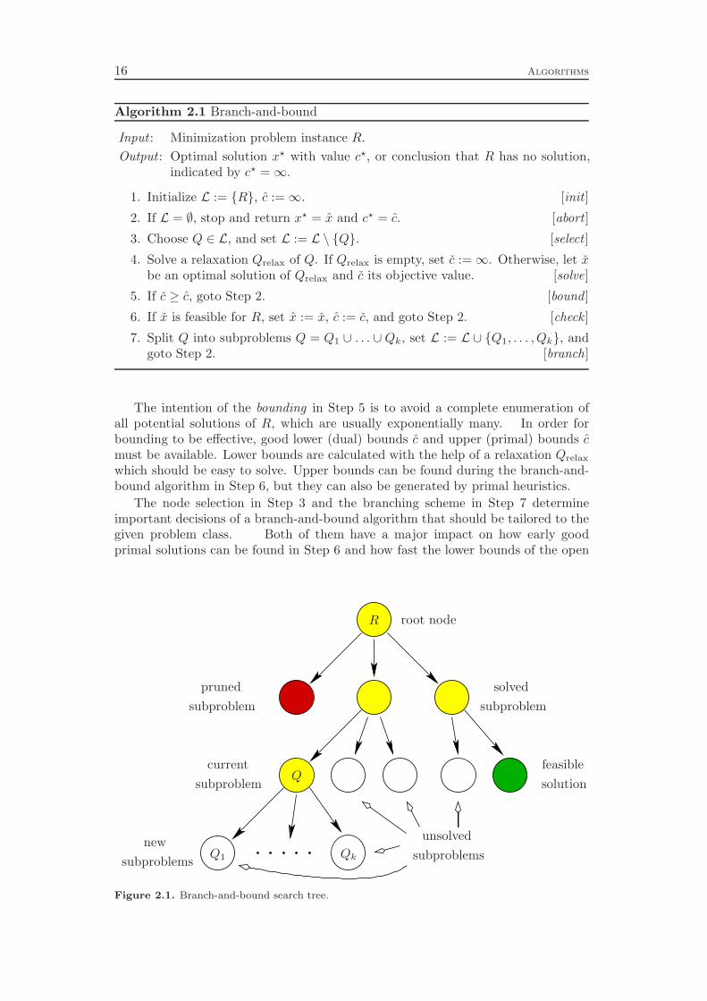
The branch-and-bound procedure is a very general and widely used method to solveoptimization problems. It is also known as implicit enumeration, divide-and-conquer,backtracking, or decomposition. The idea is to successively divide the given prob-lem instance into smaller subproblems until the individual subproblems are easy tosolve. The best of the subproblems’ solutions is the global optimum. Algorithm 2.1summarizes this procedure.
The splitting of a subproblem into two or more smaller subproblems in Step 7is called branching. During the course of the algorithm, a branching tree is createdwith each node representing one of the subproblems (see Figure 2.1). The rootof the tree corresponds to the initial problem R, while the leaves are either “easy”subproblems that have already been solved or subproblems in L that still have tobe processed.
15
16 Algorithms
Algorithm 2.1 Branch-and-bound
Input : Minimization problem instance R.
Output : Optimal solution x⋆ with value c⋆, or conclusion that R has no solution,indicated by c⋆ =∞.
1. Initialize L := {R}, c :=∞. [init ]
2. If L = ∅, stop and return x⋆ = x and c⋆ = c. [abort ]
3. Choose Q ∈ L, and set L := L \ {Q}. [select ]
4. Solve a relaxation Qrelax of Q. If Qrelax is empty, set c :=∞. Otherwise, let xbe an optimal solution of Qrelax and c its objective value. [solve]
5. If c ≥ c, goto Step 2. [bound ]
6. If x is feasible for R, set x := x, c := c, and goto Step 2. [check ]
7. Split Q into subproblems Q = Q1 ∪ . . . ∪Qk, set L := L ∪ {Q1, . . . ,Qk}, andgoto Step 2. [branch]
The intention of the bounding in Step 5 is to avoid a complete enumeration ofall potential solutions of R, which are usually exponentially many. In order forbounding to be effective, good lower (dual) bounds c and upper (primal) bounds cmust be available. Lower bounds are calculated with the help of a relaxation Qrelax
which should be easy to solve. Upper bounds can be found during the branch-and-bound algorithm in Step 6, but they can also be generated by primal heuristics.
The node selection in Step 3 and the branching scheme in Step 7 determineimportant decisions of a branch-and-bound algorithm that should be tailored to thegiven problem class. Both of them have a major impact on how early goodprimal solutions can be found in Step 6 and how fast the lower bounds of the open
R
Q
Q1 Qk
root node
pruned solved
current
subproblem
subproblem
subproblem
new unsolved
subproblemssubproblems
feasible
solution
Figure 2.1. Branch-and-bound search tree.
2.1. Branch and Bound 17
Q Q1 Q2
xx
Figure 2.2. LP based branching on a single fractional variable.
subproblems in L increase. They influence the bounding in Step 5, which shouldcut off subproblems as early as possible and thereby prune large parts of the searchtree. Even more important for a branch-and-bound algorithm to be effective is thetype of relaxation that is solved in Step 4. A reasonable relaxation must fulfill twousually opposing requirements: it should be easy to solve, and it should yield strongdual bounds.
In mixed integer programming, the most widely used relaxation is the LP relax-ation (see Definition 1.5), which proved to be very successful in practice. Currently,almost all efficient commercial and academic MIP solvers are LP relaxation basedbranch-and-bound algorithms. This includes the solvers mentioned in Section 1.3.
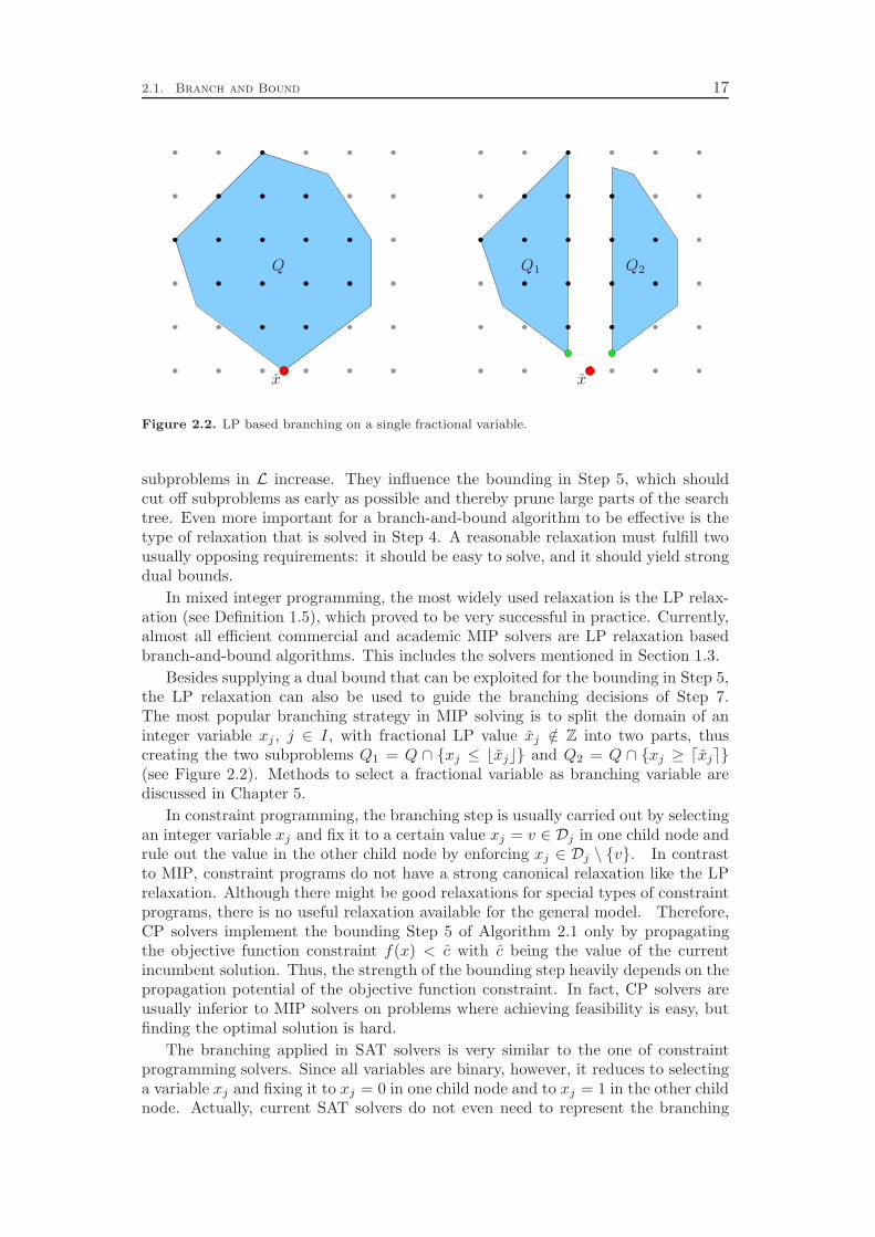
Besides supplying a dual bound that can be exploited for the bounding in Step 5,the LP relaxation can also be used to guide the branching decisions of Step 7.The most popular branching strategy in MIP solving is to split the domain of aninteger variable xj , j ∈ I, with fractional LP value xj /∈ Z into two parts, thuscreating the two subproblems Q1 = Q ∩ {xj ≤ ⌊xj⌋} and Q2 = Q ∩ {xj ≥ ⌈xj⌉}(see Figure 2.2). Methods to select a fractional variable as branching variable arediscussed in Chapter 5.
In constraint programming, the branching step is usually carried out by selectingan integer variable xj and fix it to a certain value xj = v ∈ Dj in one child node andrule out the value in the other child node by enforcing xj ∈ Dj \ {v}. In contrastto MIP, constraint programs do not have a strong canonical relaxation like the LPrelaxation. Although there might be good relaxations for special types of constraintprograms, there is no useful relaxation available for the general model. Therefore,CP solvers implement the bounding Step 5 of Algorithm 2.1 only by propagatingthe objective function constraint f(x) < c with c being the value of the currentincumbent solution. Thus, the strength of the bounding step heavily depends on thepropagation potential of the objective function constraint. In fact, CP solvers areusually inferior to MIP solvers on problems where achieving feasibility is easy, butfinding the optimal solution is hard.
The branching applied in SAT solvers is very similar to the one of constraintprogramming solvers. Since all variables are binary, however, it reduces to selectinga variable xj and fixing it to xj = 0 in one child node and to xj = 1 in the other childnode. Actually, current SAT solvers do not even need to represent the branching
18 Algorithms
Q QI
xx
Figure 2.3. A cutting plane that separates the fractional LP solution x from the convex hull QI
of integer points of Q.
decisions in a tree. Because they apply depth first search, they only need to storethe nodes on the path from the root node to the current node. This simplificationin data structures is possible since the node selection of Step 3 is performed in adepth-first fashion and conflict clauses (see Chapter 11) are generated for infeasiblesubproblems that implicitly lead the search to the opposite fixing of the branchingvariable after backtracking has been performed.
As SAT has no objective function, there is no need for the bounding Step 5 ofAlgorithm 2.1. A SAT solver can immediately abort after having found the firstfeasible solution.
2.2 Cutting Planes
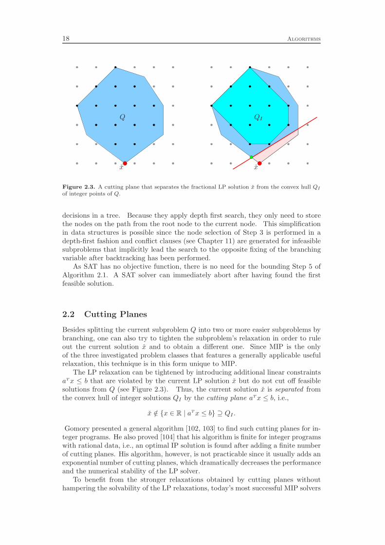
Besides splitting the current subproblem Q into two or more easier subproblems bybranching, one can also try to tighten the subproblem’s relaxation in order to ruleout the current solution x and to obtain a different one. Since MIP is the onlyof the three investigated problem classes that features a generally applicable usefulrelaxation, this technique is in this form unique to MIP.
The LP relaxation can be tightened by introducing additional linear constraintsaTx ≤ b that are violated by the current LP solution x but do not cut off feasiblesolutions from Q (see Figure 2.3). Thus, the current solution x is separated fromthe convex hull of integer solutions QI by the cutting plane aTx ≤ b, i.e.,
x /∈ {x ∈ R | aTx ≤ b} ⊇ QI .
Gomory presented a general algorithm [102, 103] to find such cutting planes for in-teger programs. He also proved [104] that his algorithm is finite for integer programswith rational data, i.e., an optimal IP solution is found after adding a finite numberof cutting planes. His algorithm, however, is not practicable since it usually adds anexponential number of cutting planes, which dramatically decreases the performanceand the numerical stability of the LP solver.
To benefit from the stronger relaxations obtained by cutting planes withouthampering the solvability of the LP relaxations, today’s most successful MIP solvers
2.3. Domain Propagation 19
combine branching and cutting plane separation in one of the following fashions:
Cut-and-branch. The LP relaxationRLP of the initial (root) problemR is strength-ened by cutting planes as long as it seems to be reasonable and does not reducenumerical stability too much. Afterwards, the problem is solved with branch-and-bound.
Branch-and-cut. The problem is solved with branch-and-bound, but the LP re-laxations QLP of all subproblems Q (including the initial problem R) might bestrengthened by cutting planes. Here one has to distinguish between globally validcuts and cuts that are only valid in a local part of the branch-and-bound search tree,i.e., cuts that were deduced by taking the branching decisions into account. Globallyvalid cuts can be used for all subproblems during the course of the algorithm, butlocal cuts have to be removed from the LP relaxation after the search leaves thesubtree for which they are valid.
Marchand et al. [154] and Fügenschuh and Martin [90] give an overview of compu-tationally useful cutting plane techniques. A recent survey of cutting plane literaturecan be found in Klar [132]. For further details, we refer to Chapter 8 and the refer-ences therein.
2.3 Domain Propagation
Constraint propagation is an integral part of every constraint programming solver.The task is to analyze the set of constraints of the current subproblem and thecurrent domains of the variables in order to infer additional valid constraints anddomain reductions, thereby restricting the search space. The special case whereonly the domains of the variables are affected by the propagation process is calleddomain propagation. If the propagation only tightens the lower and upper boundsof the domains without introducing holes it is called bound propagation or boundstrengthening.
In mixed integer programming, the concept of bound propagation is well-knownunder the term node preprocessing. One usually applies a restricted version of thepreprocessing algorithm that is used before starting the branch-and-bound processto simplify the problem instance (see, e.g., Savelsbergh [199] or Fügenschuh andMartin [90]). Besides the integrality restrictions, only linear constraints appear inmixed integer programming problems. Therefore, MIP solvers only employ a verylimited number of propagation algorithms, the most prominent being the boundstrengthening on individual linear constraints (see Section 7.1).
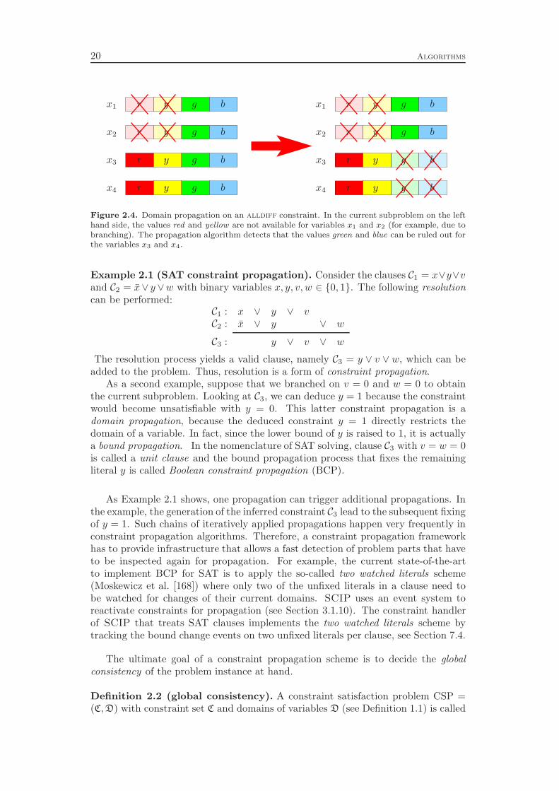
In contrast, a constraint programming model can include a large variety of con-straint classes with different semantics and structure. Thus, a CP solver providesspecialized constraint propagation algorithms for every single constraint class. Fig-ure 2.4 shows a particular propagation of the alldiff constraint, which demandsthat the involved variables have to take pairwise different values. Fast domainpropagation algorithms for alldiff constraints include the computation of maxi-mal matchings in bipartite graphs (see Régin [192]). Bound propagation algorithmsidentify so-called Hall intervals (Puget [189], López-Ortis et al. [151]).
The following example illustrates constraint propagation and domain propagationfor clauses of the satisfiability problem (see Section 1.2).
20 Algorithms
x1 x1
x2 x2
x3 x3
x4 x4
r
r
r
r
r
r
r
r
y
y
y
y
y
y
y
y
g
g
g
g
g
g
g
g
b
b
b
b
b
b
b
b
Figure 2.4. Domain propagation on an alldiff constraint. In the current subproblem on the lefthand side, the values red and yellow are not available for variables x1 and x2 (for example, due tobranching). The propagation algorithm detects that the values green and blue can be ruled out forthe variables x3 and x4.
Example 2.1 (SAT constraint propagation). Consider the clauses C1 = x∨y∨vand C2 = x∨ y∨w with binary variables x, y, v,w ∈ {0, 1}. The following resolutioncan be performed:
C1 : x ∨ y ∨ vC2 : x ∨ y ∨ w
C3 : y ∨ v ∨ w
The resolution process yields a valid clause, namely C3 = y ∨ v ∨ w, which can beadded to the problem. Thus, resolution is a form of constraint propagation.
As a second example, suppose that we branched on v = 0 and w = 0 to obtainthe current subproblem. Looking at C3, we can deduce y = 1 because the constraintwould become unsatisfiable with y = 0. This latter constraint propagation is adomain propagation, because the deduced constraint y = 1 directly restricts thedomain of a variable. In fact, since the lower bound of y is raised to 1, it is actuallya bound propagation. In the nomenclature of SAT solving, clause C3 with v = w = 0is called a unit clause and the bound propagation process that fixes the remainingliteral y is called Boolean constraint propagation (BCP).
As Example 2.1 shows, one propagation can trigger additional propagations. Inthe example, the generation of the inferred constraint C3 lead to the subsequent fixingof y = 1. Such chains of iteratively applied propagations happen very frequently inconstraint propagation algorithms. Therefore, a constraint propagation frameworkhas to provide infrastructure that allows a fast detection of problem parts that haveto be inspected again for propagation. For example, the current state-of-the-artto implement BCP for SAT is to apply the so-called two watched literals scheme(Moskewicz et al. [168]) where only two of the unfixed literals in a clause need tobe watched for changes of their current domains. SCIP uses an event system toreactivate constraints for propagation (see Section 3.1.10). The constraint handlerof SCIP that treats SAT clauses implements the two watched literals scheme bytracking the bound change events on two unfixed literals per clause, see Section 7.4.
The ultimate goal of a constraint propagation scheme is to decide the globalconsistency of the problem instance at hand.
Definition 2.2 (global consistency). A constraint satisfaction problem CSP =(C,D) with constraint set C and domains of variables D (see Definition 1.1) is called
2.3. Domain Propagation 21
globally consistent if there exists a solution x⋆ ∈ D with C(x⋆).
Since CSP is NP-complete, it is unlikely that efficient propagation schemes existthat decide global consistency. Therefore, the iterative application of constraintpropagation usually aims to achieve some form of local consistency, which is a weakerform of global consistency: a locally consistent CSP does not need to be globallyconsistent, but global consistency implies local consistency. In the following wepresent only some basic notions of local consistency that will be used in this thesis.A more thorough overview can be found in Apt [17].
Definition 2.3 (node consistency). Consider a constraint satisfaction problemCSP = (C,D) with constraint set C and domains of variables D (see Definition 1.1).A unary constraint C ∈ C on a variable xj
C : Dj → {0, 1}
is called node consistent if C(xj) = 1 for all values xj ∈ Dj . A CSP is called nodeconsistent if all of its unary constraints are node consistent.
Definition 2.4 (arc consistency). A binary constraint C ∈ C on variables xi andxj , i 6= j,
C : Di ×Dj → {0, 1},
of a constraint satisfaction problem CSP = (C,D) is called arc consistent if
∀xi ∈ Di ∃xj ∈ Dj : C(xi, xj) = 1, and
∀xj ∈ Dj ∃xi ∈ Di : C(xi, xj) = 1.
A CSP is called arc consistent if all of its binary constraints are arc consistent.
Definition 2.5 (hyper-arc consistency). An arbitrary constraint C ∈ C on vari-ables xj1 , . . . , xjk
,C : Dj1 × . . . ×Djk
→ {0, 1},
of a constraint satisfaction problem CSP = (C,D) is called hyper-arc consistent if
∀i ∈ {1, . . . , k} ∀xji∈ Dji
∃x⋆ ∈ Dj1 × . . . ×Djk: x⋆
ji= xji
∧ C(x⋆) = 1.
A CSP is called hyper-arc consistent if all of its constraints are hyper-arc consistent.
Hyper-arc consistency is the strongest possible local consistency notion withrespect to a single constraint. It demands that for each constraint C each valuein the involved domains participates in a solution which satisfies C. In other words,no further values can be excluded from the domains of the variables by consideringthe constraints individually.
An algorithm which aims to achieve hyper-arc consistency for a given constrainthas to remove all values from the domains of the involved variables that do nottake part in a solution for the constraint. For domains D ⊆ R, one usually hasto introduce holes in order to achieve hyper-arc consistency. Such algorithms canbe very time-consuming. Additionally, the LP relaxation of a constraint integerprogram can only deal with continuous intervals without holes. Therefore, we willusually regard one of the following relaxed versions of hyper-arc consistency, whichonly deal with the bounds of the interval domains:
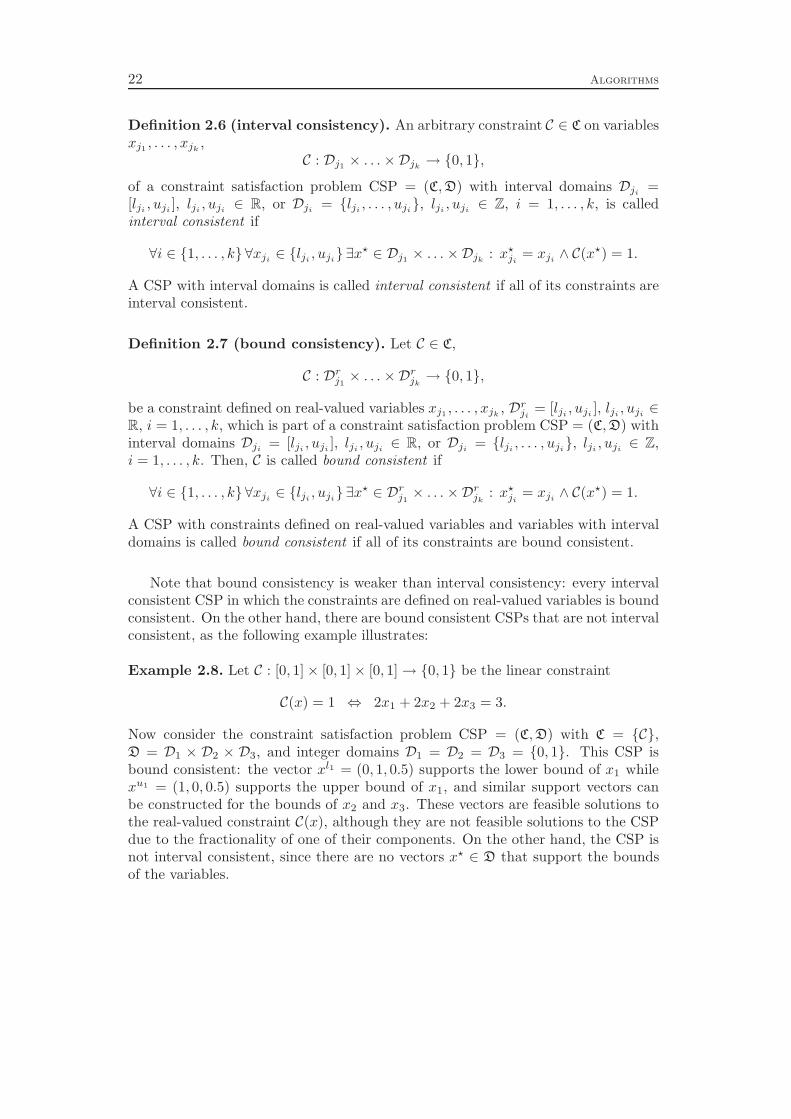
22 Algorithms
Definition 2.6 (interval consistency). An arbitrary constraint C ∈ C on variablesxj1 , . . . , xjk
,C : Dj1 × . . . ×Djk
→ {0, 1},
of a constraint satisfaction problem CSP = (C,D) with interval domains Dji=
[lji, uji
], lji, uji
∈ R, or Dji= {lji
, . . . , uji}, lji
, uji∈ Z, i = 1, . . . , k, is called
interval consistent if
∀i ∈ {1, . . . , k} ∀xji∈ {lji
, uji} ∃x⋆ ∈ Dj1 × . . . ×Djk
: x⋆ji
= xji∧ C(x⋆) = 1.
A CSP with interval domains is called interval consistent if all of its constraints areinterval consistent.
Definition 2.7 (bound consistency). Let C ∈ C,
C : Drj1× . . . ×Dr
jk→ {0, 1},
be a constraint defined on real-valued variables xj1 , . . . , xjk, Dr
ji= [lji
, uji], lji
, uji∈
R, i = 1, . . . , k, which is part of a constraint satisfaction problem CSP = (C,D) withinterval domains Dji
= [lji, uji
], lji, uji
∈ R, or Dji= {lji
, . . . , uji}, lji
, uji∈ Z,
i = 1, . . . , k. Then, C is called bound consistent if
∀i ∈ {1, . . . , k} ∀xji∈ {lji
, uji} ∃x⋆ ∈ Dr
j1× . . . ×Dr
jk: x⋆
ji= xji
∧ C(x⋆) = 1.
A CSP with constraints defined on real-valued variables and variables with intervaldomains is called bound consistent if all of its constraints are bound consistent.
Note that bound consistency is weaker than interval consistency: every intervalconsistent CSP in which the constraints are defined on real-valued variables is boundconsistent. On the other hand, there are bound consistent CSPs that are not intervalconsistent, as the following example illustrates:
Example 2.8. Let C : [0, 1]× [0, 1]× [0, 1]→ {0, 1} be the linear constraint
C(x) = 1 ⇔ 2x1 + 2x2 + 2x3 = 3.
Now consider the constraint satisfaction problem CSP = (C,D) with C = {C},D = D1 × D2 × D3, and integer domains D1 = D2 = D3 = {0, 1}. This CSP isbound consistent: the vector xl1 = (0, 1, 0.5) supports the lower bound of x1 whilexu1 = (1, 0, 0.5) supports the upper bound of x1, and similar support vectors canbe constructed for the bounds of x2 and x3. These vectors are feasible solutions tothe real-valued constraint C(x), although they are not feasible solutions to the CSPdue to the fractionality of one of their components. On the other hand, the CSP isnot interval consistent, since there are no vectors x⋆ ∈ D that support the boundsof the variables.
Chapter 3
SCIP as a CIP Framework
This chapter describes the constraint integer programming framework SCIP (anacronym for “Solving Constraint Integer Programs”). SCIP is being developed atthe Konrad-Zuse-Zentrum für Informationstechnik Berlin (ZIB) since 2001. It is thesuccessor of the mixed integer programming solver SIP of Alexander Martin [159]and adopts several ideas and algorithms of its predecessor. Nevertheless, it wasimplemented from scratch in order to obtain a much more flexible design, which iscapable of supporting constraint integer programming techniques and a wide varietyof user plugins that can be included via a callback mechanism.
Section 3.1 describes the various types of user plugins that can enrich the basicCIP framework and explains their role in the solving process. The algorithmic designand the main sequence of the solving steps are illustrated in Section 3.2. Finally,Section 3.3 covers the infrastructure which is supplied by SCIP in order to providedata structures and efficient methods to represent and access the problem data andto allow interaction and sharing of information between the plugins.
3.1 Basic Concepts of SCIP
SCIP is a constraint integer programming framework that provides the infrastruc-ture to implement very flexible branch-and-bound based search algorithms. In ad-dition, it includes a large library of default algorithms to control the search. Thesemain algorithms of SCIP are part of external plugins, which are user defined call-back objects that interact with the framework through a very detailed interface.The current distribution of SCIP contains the necessary plugins to solve MIPs (seePart II). In the following, we describe the different plugin types and their role insolving a CIP.
3.1.1 Constraint Handlers
Since a CIP consists of constraints, the central objects of SCIP are the constrainthandlers. Each constraint handler represents the semantics of a single class of con-straints and provides algorithms to handle constraints of the corresponding type.
The primary task of a constraint handler is to check a given solution for fea-sibility with respect to all constraints of its type existing in the problem instance.This feasibility test suffices to turn SCIP into an algorithm which correctly solvesCIPs with constraints of the supported type, at least if no continuous variables areinvolved. However, the resulting procedure would be a complete enumeration of allpotential solutions, because no additional information about the problem structurewould be available.
To improve the performance of the solving process constraint handlers may pro-vide additional algorithms and information about their constraints to the framework,namely
23
24 SCIP as a CIP Framework
⊲ presolving methods to simplify the problem’s representation,
⊲ propagation methods to tighten the variables’ domains,
⊲ a linear relaxation, which can be generated in advance or on the fly, thatstrengthens the LP relaxation of the problem, and
⊲ branching decisions to split the problem into smaller subproblems, using struc-tural knowledge of the constraints in order to generate a well-balanced branch-ing tree.
Example 3.1 (knapsack constraint handler). A binary knapsack constraint isa specialization of a linear constraint
aTx ≤ β (3.1)
with non-negative integral right hand side β ∈ Z≥0, non-negative integral coefficientsaj ∈ Z≥0, and binary variables xj ∈ {0, 1}, j ∈ N .
The feasibility test of the knapsack constraint handler is very simple: it onlyadds up the coefficients aj of variables xj set to 1 in the given solution and com-pares the result with the right hand side β. Presolving algorithms for knapsackconstraints include modifying the coefficients and right hand side in order to tightenthe LP relaxation, and fixing variables with aj > β to 0, see Savelsbergh [199] andSection 10.2.
The propagation method fixes additional variables to 0, that would not fit intothe knapsack together with the variables that are already fixed to 1 in the currentsubproblem.
The linear relaxation of the knapsack constraint initially consists of the knapsackinequality (3.1) itself. Additional cutting planes like lifted cover cuts (see, forexample, Balas [28], Balas and Zemel [35] or Martin and Weismantel [160]) or GUBcover cuts (see Wolsey [217]) are dynamically generated to enrich the knapsack’srelaxation and to cut off the current LP solution; see also Section 8.1.
Example 3.2 (nosubtour constraint handler). The symmetric traveling sales-man problem (TSP) on a graph G = (V,E) with edge lengths cuv ∈ R≥0, uv ∈ E,can be stated as a constraint integer program in the following way:
min∑
uv∈E
cuv xuv
s.t.∑
u∈δ(v)
xuv = 2 for all v ∈ V (3.2)
nosubtour(G,x) (3.3)
xuv ∈ {0, 1} for all uv ∈ E (3.4)
Formally, this model consists of |V | degree constraints (3.2), one nosubtour con-straint (3.3), and |E| integrality constraints (3.4). The nosubtour constraint is anon-linear constraint which is defined as
nosubtour(G,x) ⇔ ∄C ⊆ {uv ∈ E | xuv = 1} : C is a cycle of length |C| < |V |.
This constraint must be supported by a constraint handler, which for a given integralsolution x ∈ {0, 1}E checks whether the corresponding set of edges contains a subtour
3.1. Basic Concepts of SCIP 25
C. The linear relaxation of the nosubtour constraint consists of exponentiallymany subtour elimination inequalities
∑
uv∈E(S)
xuv ≤ |S| − 1 for all S ⊂ V with 2 ≤ |S| ≤ |V | − 2,
which can be separated and added on demand to the LP relaxation. Additionally,the constraint handler could separate various other classes of valid inequalities forthe traveling salesman problem that can be found in the literature, see, for exam-ple, Grötschel and Padberg [108, 109], Grötschel and Holland [107], Clochard andNaddef [62], Applegate et al. [14, 15, 16], or Naddef [169].
3.1.2 Presolvers
In addition to the constraint based (primal) presolving mechanisms provided by theindividual constraint handlers, additional presolving algorithms can be applied withthe help of presolvers, which interact with the whole set of constraints. They may,for example, perform dual presolving reductions which take the objective functioninto account.
For instance, if the value of a variable xj can always be decreased without ren-dering any constraint infeasible (an information, the constraint handlers have toprovide by setting variable locks, see Section 3.3.3), and if the objective value cj ofthe variable is non-negative, the dual fixing presolver fixes the variable to its lowerbound, see Section 10.8. In the setting of an MIP with inequality system Ax ≤ b,this condition is satisfied if and only if A·j ≥ 0 and cj ≥ 0.1
3.1.3 Cut Separators
In SCIP, we distinguish between two different types of cutting planes. The first typeare the constraint based cutting planes, that are valid inequalities or even facets ofthe polyhedron described by a single constraint or a subset of the constraints of asingle constraint class. These cutting planes may also be strengthened by liftingprocedures that take information about the full problem into account, for examplethe implication graph, see Section 3.3.5. They are generated by the constraint han-dlers of the corresponding constraint types. Prominent examples are the differenttypes of knapsack cuts that are generated in the knapsack constraint handler, seeExample 3.1, or the cuts for the traveling salesman problem like subtour elimina-tion and comb inequalities which can be separated by the nosubtour constrainthandler, see Example 3.2.
The second type of cutting planes are general purpose cuts, which are using thecurrent LP relaxation and the integrality conditions to generate valid inequalities.Generating those cuts is the task of cut separators. Examples are Gomory fractionaland Gomory mixed integer cuts (Gomory [104]), complemented mixed integer round-ing cuts (Marchand and Wolsey [155]), and strong Chvátal-Gomory cuts (Letchfordand Lodi [142]).
3.1.4 Domain Propagators
Like for cutting planes, there are two different types of domain propagations. Con-straint based (primal) domain propagation algorithms are part of the correspond-
1Here, A·j is the j’th column of the coefficient matrix A.
26 SCIP as a CIP Framework
ing constraint handlers. For example, the alldiff2 constraint handler excludescertain values of the variables’ domains with the help of a bipartite matching algo-rithm, see Regin [192], or applies bound propagation by so-called Hall intervals, seeLeconte [140], Puget [189], or López-Ortiz et al. [151].
In contrast, domain propagators provide dual propagations, i.e., propagationsthat can be applied due to the objective function and the currently best known primalsolution. An example is the simple objective function propagator of Section 7.6 thattightens the variables’ domains with respect to the objective bound
cTx < c
with c being the objective value of the currently best primal solution.
3.1.5 Variable Pricers
Several optimization problems are modeled with a huge number of variables, e.g.,with each path in a graph or each subset of a given set corresponding to a singlevariable. In this case, the full set of variables cannot be generated in advance.Instead, the variables are added dynamically to the problem whenever they mayimprove the current solution. In mixed integer programming, this technique iscalled column generation.
SCIP supports dynamic variable creation by variable pricers. They are calledduring the subproblem processing and have to generate additional variables thatreduce the lower bound of the subproblem. If they operate on the LP relaxation,they would usually calculate the reduced costs of the not yet existing variables with aproblem specific algorithm and add some or all of the variables with negative reducedcosts. Note that since variable pricers are part of the model, they are always problemclass specific. Therefore, SCIP does not contain any “default” variable pricers.
3.1.6 Branching Rules
If the LP solution of the current subproblem is fractional, the integrality constrainthandler calls the branching rules to split the problems into subproblems. Addition-ally, branching rules are called as a last resort on integral solutions that violate oneor more constraints for which the associated constraint handlers were not able toresolve the infeasibility in a more sophisticated way, see Section 3.2.8.
Usually, a branching rule creates two subproblems by splitting a single variable’sdomain. If applied on a fractional LP solution, commonly an integer variable xj
with fractional value xj is selected, and the two branches xj ≤ ⌊xj⌋ and xj ≥ ⌈xj⌉are created. The well-known most infeasible, pseudocost, reliability, and strongbranching rules are examples of this type (see Achterberg, Martin, and Koch [5] andChapter 5). It is also possible to implement much more general branching schemes,for example by creating more than two subproblems, or by adding additional con-straints to the subproblems instead of tightening the domains of the variables.
3.1.7 Node Selectors
Node selectors decide which of the leaves in the current branching tree is selectedas next subproblem to be processed. This choice can have a large impact on the
2alldiff(x1, . . . , xk) requires the integer variables x1, . . . , xk to take pairwise different values.
3.1. Basic Concepts of SCIP 27
solver’s performance, because it influences the finding of feasible solutions and thedevelopment of the global dual bound.
Constraint programming was originally developed for constraint satisfaction prob-lems (CSPs). In this setting, the solver only has to check whether there is a feasiblesolution or not. Therefore, many of the available CP solvers employ depth firstsearch. The same holds for the satisfiability problem. SAT solvers are even moretailored to depth first search, since one of their key components—conflict analysis(see Chapter 11)—is best suited for the use inside a depth first search algorithm. Amore extensive discussion of this topic can be found in Section 16.2.
With the addition of an objective function, depth first search is usually an inferiorstrategy. It tends to evaluate many nodes in the tree that could have been discardedif a good or optimal solution were known earlier. In mixed integer programming,several node selection strategies are known that try to discover good feasible solutionsearly during the search process. Examples of those strategies are best first and bestestimate search. See Chapter 6 for a comparison of node selection strategies forMIP.
3.1.8 Primal Heuristics
Feasible solutions can be found in two different ways during the traversal of thebranching tree. On the one hand, the solution of a node’s relaxation may be feasiblew.r.t. the constraints. On the other hand, feasible solutions can be discovered byprimal heuristics. They are called periodically during the search.
SCIP provides specific infrastructure for diving and probing heuristics. Div-ing heuristics iteratively resolve the LP after making a few changes to the currentsubproblem, usually aiming at driving the fractional values of integer variables tointegrality. Probing heuristics are even more sophisticated. Besides solving LPrelaxations, they may call the domain propagation algorithms of the constraint han-dlers after applying changes to the variables’ domains, and they can undo thesechanges using backtracking.
Other heuristics without special support in SCIP include local search heuristicslike tabu search [97], rounding heuristics which try to round the current fractionalLP solution to a feasible integral solution, and improvement heuristics like localbranching [85] or RINS [72], which try to generate improved solutions by inspectingone or more of the feasible solutions that have already been found. Chapter 9provides an overview of the heuristics included in SCIP to solve mixed integerprograms.
3.1.9 Relaxation Handlers
SCIP provides specific support for LP relaxations: constraint handlers implementcallback methods for generating the LP, additional cut separators may be included tofurther tighten the LP relaxation, and there are a lot of interface methods availableto access the LP information at the current subproblem.
In addition, it is also possible to include other relaxations, e.g., Lagrange re-laxations or semidefinite relaxations. This is possible through relaxation handlerplugins. The relaxation handler manages the necessary data structures and calls therelaxation solver to generate dual bounds and primal solution candidates. However,the data to define a single relaxation must either be extracted by the relaxationhandler itself (e.g., from the user defined problem data, the LP information, or the
28 SCIP as a CIP Framework
integrality conditions), or be provided by the constraint handlers. In the latter case,the constraint handlers have to be extended to support this specific relaxation.
Like with LP relaxations, support for managing warm start information is avail-able to speed up the resolves at the subproblems. At each subproblem, the usermay solve any number of relaxations, including the LP relaxation. In particular, itis possible to refrain from solving any relaxation, in which case SCIP behaves likea CP solver.
3.1.10 Event Handlers
SCIP contains a sophisticated event system, which can be used by external pluginsto be informed about certain events. These events are processed by event handlerplugins. Usually, the event handlers pass the information to other objects, e.g., toa constraint handler. It is very common in SCIP that a constraint handler closelyinteracts with an event handler in order to improve its own runtime performance.
For example, a constraint handler may want to be informed about the domainchanges of the variables involved in its constraints. This can be used to avoidunnecessary work in preprocessing and propagation: a constraint has only to beprocessed again, if at least one domain of the involved variables was changed sincethe last preprocessing or propagation call. Events can also be used to update certaininternal values (e.g., the total weight of variables currently fixed to 1 in a knapsackconstraint) in order to avoid frequent recalculations.
Other potential applications for the event system include a dynamic graphicaldisplay of the currently best solution and the online visualization of the branchingtree. These are supported by events triggered whenever a new primal solution hasbeen found or a node has been processed.
3.1.11 Conflict Handlers
Current state-of-the-art SAT solvers employ analysis of infeasible subproblems togenerate so-called conflict clauses (see Marques-Silva and Sakallah [157]). These areimplied constraints that may help to prune the branching tree. In the CP community,a generalization of those clauses is known as no-goods.
SCIP adopts this mechanism and extends it to the analysis of infeasible LPs, seeChapter 11. Whenever a conflict was found by the internal analysis algorithms, theincluded conflict handlers are called to create a conflict constraint out of the set ofconflicting variables. Conflict handlers usually cooperate with constraint handlersby calling the constraint creation method of the constraint handler and adding theconstraint to the model.
3.1.12 File Readers
File readers are called to parse an input file and generate a CIP model. They createconstraints and variables and activate variable pricers if necessary. Each file readeris hooked to a single file name extension. It is automatically called if the user wantsto read in a problem file of corresponding name. Examples of file formats arethe MPS format [117] and the Cplex LP format [118] for linear and mixed integerprograms, the CNF format for SAT instances in conjunctive normal form, and theTSP format [193] for instances of the traveling salesman problem.

3.2. Algorithmic Design 29
Init
ProblemSpecification
Transforming
Transformed
Presolving
Presolved
Init Solve
SolvingSolved
Free Solve
Free Transform
Figure 3.1. Operational stages of SCIP. The arrows represent possible transitions between stages.
3.1.13 Display Columns
While solving a constraint integer program, SCIP displays status information in acolumn-like fashion. The current number of processed branching tree nodes, thesolving time, and the relative gap between primal and dual bound are examples ofsuch display columns. There already exists a wide variety of display columns whichcan be activated or deactivated on demand. Additionally, the user can implementhis own display columns in order to track problem or algorithm specific values.
3.1.14 Dialog Handlers
SCIP comes with a command line shell which allows the user to read in probleminstances, modify the solver’s parameters, initiate the optimization, and displaycertain statistics and solution information. This shell can be extended by dialoghandlers. They are linked to the shell’s calling tree and executed whenever theuser enters the respective command. The default shell itself is also generated bydialog handlers and is therefore completely adjustable to the needs of the softwaredeveloper.
3.1.15 Message Handlers
All screen output of SCIP is passed through a message handler. By overwriting theappropriate callback methods, the user can easily redirect or suppress the output.
3.2 Algorithmic Design
Figure 3.1 shows a flow chart of the main operational stages that are traversed duringthe execution of SCIP. In this section we specify which callback methods of thedifferent plugins are executed and which operations the user may perform duringthe different stages. It is explained how the problem is represented in SCIP’s data
30 SCIP as a CIP Framework
structures and which transformations are being applied during the course of thealgorithm. Compare also the data flow illustrated in Figure 3.5 on page 37.
3.2.1 Init Stage
In the init stage, the basic data structures are allocated and initialized. The user hasto include the required plugins with calls to the SCIPinclude...() methods. Eachincluded plugin may allocate its own private data. With a call to SCIPcreateProb()
or SCIPreadProb(), the solver leaves the init stage and enters the problem specifi-cation stage, the latter one executing a file reader to create the problem instance.
3.2.2 Problem Specification Stage
During the problem specification stage, the user can define and modify the originalproblem instance that he wants to solve. He can create constraints and variablesand activate included variable pricers. A file reader that is called during the initstage switches to the problem specification stage with a call to SCIPcreateProb()
and subsequently creates the necessary problem data.
3.2.3 Transforming Stage
Before the actual solving process begins, SCIP creates a working copy of the orig-inal problem instance. The working copy is called the transformed problem andprotects the original problem instance from modifications applied during presolvingor solving. The original problem can only be modified in the problem specificationstage.
In the transforming stage, the data of variables and constraints are copied intoa separate memory area. Because SCIP does not know how the constraints arerepresented, it has to call the constraint handlers to create copies of their constraints.
3.2.4 Transformed Stage
After the copying process of the transforming stage is completed, the transformedstage is reached. This state is only an intermediate state, from which the user mayinitiate the presolving stage or free the solving process data by switching into thefree transform stage.
3.2.5 Presolving Stage
In the presolving stage, permanent problem modifications on the transformed prob-lem are applied by the presolvers and the presolving methods of the constrainthandlers. These plugins are called iteratively until no more reductions can be foundor until a specified limit is reached.
One of the main tasks of presolving is to detect fixings and aggregations ofvariables, which are stored in the variable aggregation graph, see Section 3.3.4. Fixedand aggregated variables are deleted from the transformed problem and replaced bytheir fixed value or their representing active variables, respectively.
Constraint handlers may also upgrade their constraints to a more specific con-straint type. For example, as explained in Section 10.1, the linear constraint handler

3.2. Algorithmic Design 31
provides an upgrading mechanism for its constraints
β ≤ aTx ≤ β.
Other constraint handlers can be hooked into this mechanism to be called for convert-ing linear constraints into constraints of their own type. For example, the knapsackconstraint handler (see Example 3.1) checks whether the linear constraint consists ofonly binary variables, integral weights, and only one finite side β or β. If the checksucceeds, the linear constraint is converted into a knapsack constraint, possibly bynegating some of the binary variables or inverting the inequality. Such an upgrad-ing of a constraint into a more specific type has the advantage that the specializedconstraint handler can store the constraint data in a more compact form and canemploy specialized, more efficient algorithms.
3.2.6 Presolved Stage
Like the transformed stage, the presolved stage is an intermediate stage, which isreached after the presolving is completed. Thereafter, the actual solving processmay be launched. If the presolving already solved the problem instance by detectinginfeasibility or unboundness or by fixing all variables, SCIP automatically switchesvia the init solve stage to the solved stage.
3.2.7 Init Solve Stage
In the init solve stage all necessary data structures for the solving process are setup. For example, the root node of the branching tree is created and the LP solver isinitialized. Additionally, the plugins are informed about the beginning of the solvingprocess in order to enable them to create and initialize their private data.
3.2.8 Solving Stage
If the problem was not already solved in the presolving stage, the branch-and-boundprocess is performed in the solving stage to implicitly enumerate the potential so-lutions. This stage contains the main solving loop of SCIP which consists of fivedifferent steps that are called successively until the problem is solved or the solvingprocess is interrupted (see Figure 3.2).
Node Selection
The first step of each iteration in the main solving loop is the selection of thenext subproblem. The node selector of highest priority (the active node selector) iscalled to select one of the leaves in the branching tree to be processed. It can decidebetween the current node’s children and siblings, and the “best” of the remainingleaves stored in the tree. The ordering relation of the tree’s leaves is also defined bythe active node selector.
Successively choosing a child or sibling of the current node is called plunging ordiving. Selecting the best leaf of the tree ends the current plunging sequence andstarts the next one. During plunging, the setup of the subproblems to be processedis computationally less expensive, since the children and siblings are most likely tobe closely related to the current node. Switching to the best leaf of the tree is more
32 SCIP as a CIP Framework
Node Selection
Primal Heuristics
Primal Heuristics
Primal Heuristics
Domain Propagation
Relaxation Solving
Constraint Enforcement
Figure 3.2. Main solving loop of the solving stage.
expensive, but has the advantage that the search can be brought to regions in thesearch space that are more promising to contain feasible solutions of small objectivevalue—at least if the ordering of the leaves corresponds to the subproblems’ dual(i.e., lower) bounds. Additionally, it helps to improve the global dual bound morequickly. Efficient node selectors for MIP employ a mixture of plunging and best firstsearch. SAT and CSP solvers usually perform depth first search since these twoproblems are pure feasibility problems, which do not contain an objective function.
SCIP has two different operation modes: the standard mode and the memorysaving mode. If the memory limit—given as a parameter by the user—is nearlyreached, SCIP switches to the memory saving mode in which different prioritiesfor the node selectors are applied. Usually, the depth first search node selectorhas highest priority in memory saving mode, since it does not produce as manyunprocessed nodes as strategies like best first search and tends to reduce the numberof open leaves, thereby releasing allocated memory. If the memory consumptiondecreased sufficiently, SCIP switches back to standard mode.
Primal Heuristics
Primal heuristics have different entry points during the solving process. If applicable,a primal heuristic can be called directly after the next subproblem to be processed isselected. This is particularly useful for heuristics that do not need to access the LPsolution of the current node. If such a heuristic finds a feasible solution, the leavesof the branching tree exceeding the new primal bound are pruned. It may happenthat even the current node can be cut off without solving the LP relaxation. Veryfast heuristics that require an LP solution can also be called during the “RelaxationSolving” loop, see below. Most heuristics, however, are called either after the LPrelaxation was solved or after the node has been completely processed, which meansthat the node was either cut off or a branching was applied.
Like most plugins in SCIP, primal heuristics do not need to be executed at every
3.2. Algorithmic Design 33
Node Selection
Primal Heuristics
Primal Heuristics
Primal Heuristics
Domain Propagation
Constraint Enforcement
LP Solving
Calling LP Solver
Variable Pricing
Cut Separation
Figure 3.3. Main solving loop of the solving stage with detailed LP solving loop.
single node. They are usually called with a certain frequency, i.e., at specific depthlevels in the branching tree, with the more expensive heuristics being called lessoften.
Domain Propagation
After a node is selected to be processed, the corresponding subproblem is set up,and the applicable primal heuristics have been called, the domain propagators andthe domain propagation methods of the constraint handlers are called to tightenthe variables’ local domains. This propagation is applied iteratively until no morereductions are found or a propagation limit set by the user is reached. Domainpropagation does not have to be applied at every node. Every constraint handlerand domain propagator can decide whether it wants to invest the effort of trying totighten the variables’ domains.
Relaxation Solving
The next step of the solving loop is to solve the subproblem’s relaxations, in par-ticular the LP relaxation. Like domain propagation, the solving of relaxations canbe skipped or applied as needed. If there are active variable pricers, however, theLP relaxation has to be solved in order to generate new variables and to obtain afeasible dual bound.
The LP solving consists of an inner loop as can be seen in Figure 3.3. It isexecuted as long as changes to the LP have been applied in the variable pricing orcut separation steps.
Calling LP Solver. The first step is to call the LP solver to solve the initial LPrelaxation of the subproblem. In the root node, this is defined by the relaxations ofconstraints that are marked to be initial : the constraint handlers are asked to enrich
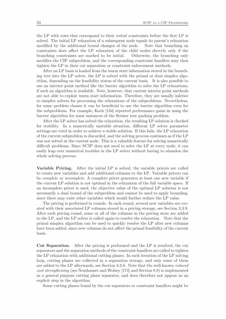
34 SCIP as a CIP Framework
the LP with rows that correspond to their initial constraints before the first LP issolved. The initial LP relaxation of a subsequent node equals its parent’s relaxationmodified by the additional bound changes of the node. Note that branching onconstraints does affect the LP relaxation of the child nodes directly only if thebranching constraints are marked to be initial. Otherwise, the branching onlymodifies the CIP subproblem, and the corresponding constraint handlers may thentighten the LP in their cut separation or constraint enforcement methods.
After an LP basis is loaded from the warm start information stored in the branch-ing tree into the LP solver, the LP is solved with the primal or dual simplex algo-rithm, depending on the feasibility status of the current basis. It is also possible touse an interior point method like the barrier algorithm to solve the LP relaxations,if such an algorithm is available. Note, however, that current interior point methodsare not able to exploit warm start information. Therefore, they are usually inferiorto simplex solvers for processing the relaxations of the subproblems. Nevertheless,for some problem classes it can be beneficial to use the barrier algorithm even forthe subproblems. For example, Koch [134] reported performance gains in using thebarrier algorithm for some instances of the Steiner tree packing problem.
After the LP solver has solved the relaxation, the resulting LP solution is checkedfor stability. In a numerically unstable situation, different LP solver parametersettings are tried in order to achieve a stable solution. If this fails, the LP relaxationof the current subproblem is discarded, and the solving process continues as if the LPwas not solved at the current node. This is a valuable feature for solving numericallydifficult problems. Since SCIP does not need to solve the LP at every node, it caneasily leap over numerical troubles in the LP solver without having to abandon thewhole solving process.
Variable Pricing. After the initial LP is solved, the variable pricers are calledto create new variables and add additional columns to the LP. Variable pricers canbe complete or incomplete. A complete pricer generates at least one new variable ifthe current LP solution is not optimal in the relaxation of the full variable space. Ifan incomplete pricer is used, the objective value of the optimal LP solution is notnecessarily a dual bound of the subproblem and cannot be used to apply bounding,since there may exist other variables which would further reduce the LP value.
The pricing is performed in rounds. In each round, several new variables are cre-ated with their associated LP columns stored in a pricing storage, see Section 3.3.9.After each pricing round, some or all of the columns in the pricing store are addedto the LP, and the LP solver is called again to resolve the relaxation. Note that theprimal simplex algorithm can be used to quickly resolve the LP after new columnshave been added, since new columns do not affect the primal feasibility of the currentbasis.
Cut Separation. After the pricing is performed and the LP is resolved, the cutseparators and the separation methods of the constraint handlers are called to tightenthe LP relaxation with additional cutting planes. In each iteration of the LP solvingloop, cutting planes are collected in a separation storage, and only some of themare added to the LP afterwards, see Section 3.3.8. Note that the well-known reducedcost strengthening (see Nemhauser and Wolsey [174] and Section 8.8) is implementedas a general purpose cutting plane separator, and does therefore not appear as anexplicit step in the algorithm.
Some cutting planes found by the cut separators or constraint handlers might be

3.2. Algorithmic Design 35
simple bound changes, i.e., cuts with only one non-zero coefficient. In particular, thereduced cost strengthening cut separator produces inequalities of this type. Needlessto say, such trivial cuts are not added as rows to the LP, but modify the localbounds of the variables directly. If bound changes have been applied, the domainpropagation is called again with the hope to tighten even more bounds. If no boundchanges, but other cutting planes have been found, the LP is resolved. The dualsimplex algorithm can be applied efficiently, since added rows and modified boundsdo not affect the dual feasibility of the current basis. If no cutting planes have beengenerated, the LP solving loop is finished, and the applicable primal heuristics arecalled.
Constraint Enforcement
After the domain propagation has been applied and the relaxations are solved, theconstraint handlers are asked to process one of the relaxations’ primal solutions.In MIP, they usually use the solution of the LP relaxation.
In contrast to the constraint handlers’ feasibility tests, which only check a givenprimal solution (generated by a primal heuristic) for feasibility, the enforcementmethods should also try to resolve an infeasibility. The constraint handler has dif-ferent options of dealing with an infeasibility (see Figure 3.4):
⊲ reducing a variable’s domain to exclude the infeasible solution from the localset of domains,
⊲ adding an additional valid constraint that can deal appropriately with theinfeasible solution,
⊲ adding a cutting plane to the LP relaxation that cuts off the infeasible solution,
⊲ creating a branching with the infeasible solution no longer being feasible in therelaxations of the child nodes,
⊲ concluding that the current subproblem is infeasible as a whole and can bepruned from the branching tree,
⊲ stating that the solution is infeasible without resolving the infeasibility.
Constraint handlers can also answer that the current solution is feasible for all of itsconstraints.
The constraint handlers’ enforcement methods are called in an order specifiedby the constraint handlers’ enforcement priorities. Depending on the result of eachconstraint enforcement method, SCIP proceeds differently. If the constraint handlertightened a variable’s domain or added a constraint, the enforcement cycle is abortedand the algorithm jumps back to domain propagation. Adding a cutting planeinvokes the LP solving again. Branching and pruning the current node finishes theprocessing of the node after which the primal heuristics are called. If the constrainthandler detects the solution to be infeasible without resolving it, or if the solutionis feasible for the constraints of the constraint handler, the next constraint handleris asked to process the current solution.
The constraint enforcement cycle can have three different outcomes:
1. A constraint handler has resolved an infeasibility, after which the node pro-cessing is continued appropriately.
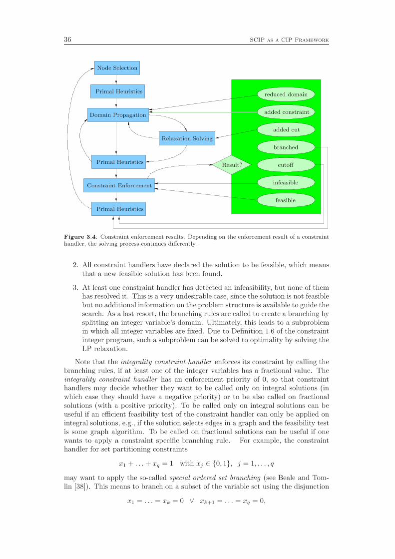
36 SCIP as a CIP Framework
Node Selection
Primal Heuristics
Primal Heuristics
Primal Heuristics
Domain Propagation
Relaxation Solving
Constraint Enforcement
Result?
reduced domain
added constraint
added cut
branched
cutoff
infeasible
feasible
Figure 3.4. Constraint enforcement results. Depending on the enforcement result of a constrainthandler, the solving process continues differently.
2. All constraint handlers have declared the solution to be feasible, which meansthat a new feasible solution has been found.
3. At least one constraint handler has detected an infeasibility, but none of themhas resolved it. This is a very undesirable case, since the solution is not feasiblebut no additional information on the problem structure is available to guide thesearch. As a last resort, the branching rules are called to create a branching bysplitting an integer variable’s domain. Ultimately, this leads to a subproblemin which all integer variables are fixed. Due to Definition 1.6 of the constraintinteger program, such a subproblem can be solved to optimality by solving theLP relaxation.
Note that the integrality constraint handler enforces its constraint by calling thebranching rules, if at least one of the integer variables has a fractional value. Theintegrality constraint handler has an enforcement priority of 0, so that constrainthandlers may decide whether they want to be called only on integral solutions (inwhich case they should have a negative priority) or to be also called on fractionalsolutions (with a positive priority). To be called only on integral solutions can beuseful if an efficient feasibility test of the constraint handler can only be applied onintegral solutions, e.g., if the solution selects edges in a graph and the feasibility testis some graph algorithm. To be called on fractional solutions can be useful if onewants to apply a constraint specific branching rule. For example, the constrainthandler for set partitioning constraints
x1 + . . . + xq = 1 with xj ∈ {0, 1}, j = 1, . . . , q
may want to apply the so-called special ordered set branching (see Beale and Tom-lin [38]). This means to branch on a subset of the variable set using the disjunction
x1 = . . . = xk = 0 ∨ xk+1 = . . . = xq = 0,
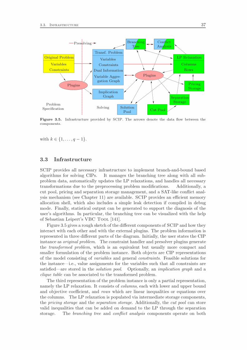
3.3. Infrastructure 37
Original ProblemVariables
Variables Constraints
Constraints
Transf. Problem
Dual Information
Variable Aggre-gation Graph
ImplicationGraph
BranchingTree
ConflictAnalysis
LP Relaxation
Columns
Rows
PricingStorage
StorageSeparation
SolutionPool
Cut Pool
Plugins
Plugins
ProblemSpecification
Presolving
Solving
Figure 3.5. Infrastructure provided by SCIP. The arrows denote the data flow between thecomponents.
with k ∈ {1, . . . , q − 1}.
3.3 Infrastructure
SCIP provides all necessary infrastructure to implement branch-and-bound basedalgorithms for solving CIPs. It manages the branching tree along with all sub-problem data, automatically updates the LP relaxations, and handles all necessarytransformations due to the preprocessing problem modifications. Additionally, acut pool, pricing and separation storage management, and a SAT-like conflict anal-ysis mechanism (see Chapter 11) are available. SCIP provides an efficient memoryallocation shell, which also includes a simple leak detection if compiled in debugmode. Finally, statistical output can be generated to support the diagnosis of theuser’s algorithms. In particular, the branching tree can be visualized with the helpof Sebastian Leipert’s VBC Tool [141].
Figure 3.5 gives a rough sketch of the different components of SCIP and how theyinteract with each other and with the external plugins. The problem information isrepresented in three different parts of the diagram. Initially, the user states the CIPinstance as original problem. The constraint handler and presolver plugins generatethe transformed problem, which is an equivalent but usually more compact andsmaller formulation of the problem instance. Both objects are CIP representationsof the model consisting of variables and general constraints. Feasible solutions forthe instance—i.e., value assignments for the variables such that all constraints aresatisfied—are stored in the solution pool. Optionally, an implication graph and aclique table can be associated to the transformed problem.
The third representation of the problem instance is only a partial representation,namely the LP relaxation. It consists of columns, each with lower and upper boundand objective coefficient, and rows which are linear inequalities or equations overthe columns. The LP relaxation is populated via intermediate storage components,the pricing storage and the separation storage. Additionally, the cut pool can storevalid inequalities that can be added on demand to the LP through the separationstorage. The branching tree and conflict analysis components operate on both
38 SCIP as a CIP Framework
representations, the CIP model of the transformed problem and the LP relaxation.The user plugins can access all of the components, although the LP relaxation canonly be modified through the pricing and separation storages.
The following sections take a closer look at the different components and describetheir role in the solving process and their interaction with the user plugins.
3.3.1 Original Problem
The original problem stores the data of the problem instance as it was entered bythe user. It consists of variables and constraints. Each variable xj has an objectivefunction coefficient cj ∈ R, a lower bound lj ∈ R and an upper bound uj ∈ R.Additionally, it is known whether the variable is of integer or continuous type. Incontrast to this explicit information about the variables, the constraints are justabstract data objects. To define their semantics, the user has to provide exter-nal plugins (constraint handlers) for each class of constraints. SCIP calls theseconstraint handlers through a callback interface at different points in the solvingprocess, see Section 3.1.1.
3.3.2 Transformed Problem
The transformed problem is created as a direct copy of the original problem. Whilethe original problem instance is retained in a separate data area, the transformedproblem is modified in the presolving and solving steps of SCIP. For example,variables and constraints of the transformed problem can be eliminated or replaced,the domains of variables can be tightened, or the constraint data can be altered.Nevertheless, the transformed problem remains equivalent to the original problemin the sense that the transformed problem is feasible if and only if the originalproblem is feasible, and that every feasible (optimal) solution of the transformedproblem can be converted into a feasible (optimal) solution of the original problem.
3.3.3 Dual Information
One main drawback of the abstract constraint approach of SCIP is the inaccessibilityof dual information about the variables. For example, a component like a presolvingplugin cannot answer the question in which constraints a variable appears, since thedata of the constraints are private to the corresponding constraint handler.
To remedy this situation, SCIP requires the constraint handlers to provide atleast a minimum of dual information which is stored in the data structures of thevariables. This information consists of the number of down-locks and up-locks foreach variable.
Definition 3.3 (variable locks). Let Ci : Rn → {0, 1} be a constraint of a con-straint integer program CIP = (C, I, c). We say that Ci down-locks (up-locks) xj
if there exist two vectors x, x ∈ Rn with Ci(x) = 1, Ci(x) = 0, xk = xk for allk 6= j, xj , xj ∈ Z if j ∈ I, and xj < xj (xj > xj). The number of constraints whichdown-lock and up-lock variable xj is denoted by ζ−j and ζ+
j , respectively.
The variable locks ζ−j and ζ+j can be interpreted as the number of constraints
that “block” the shifting of xj in direction to its lower or upper bound.
3.3. Infrastructure 39
Example 3.4 (variable locks for inequality systems). For a mixed integerprogram with constraint system Ax ≤ b, the variable lock numbers are given by thenumber of negative and positive coefficients per column: ζ−j = |{i | Aij < 0}| and
ζ+j = |{i | Aij > 0}|.
Example 3.5 (variable locks for general constraints). Consider the constraintinteger program
C1 : 3x1 +5x2− 2x3 +x4− 2x5 ≤ 8
C2 : 4x3 +3x5 = 5
C3 : alldiff( x1 , x2 , x3 )
with variables x1, x2, x3 ∈ Z≥0 and x4, x5 ∈ R≥0. The linear inequality C1 down-locks x3 and x5, and up-locks x1, x2, and x4. The equation C2 down-locks andup-locks both involved variables, x3 and x5. The alldiff constraint C3 also down-and up-locks its variables, i.e., x1, x2, and x3. The resulting lock numbers areζ−1 = 1, ζ+
1 = 2, ζ−2 = 1, ζ+2 = 2, ζ−3 = 3, ζ+
3 = 2, ζ−4 = 0, ζ+4 = 1, ζ−5 = 2, ζ+
5 = 1.Most interestingly, variable x4 has no down-locks. If its objective function coefficientc4 is non-negative, we can fix it to its lower bound. This reduction does not alter thefeasibility status of the instance, and if the instance is feasible it preserves at leastone optimal solution. It is performed by the dual fixing plugin, see Section 10.8.
3.3.4 Variable Aggregation
One of the main operations to simplify the transformed problem during presolving isthe fixing and aggregation of variables. This can delete variables from the problemby replacing their occurrences in the constraints with the corresponding counterpart,either a fixed value or an affine linear combination of active problem variables. Thefixings and aggregations are stored in a variable aggregation graph, which is usedby the framework to automatically convert any operations on those variables toequivalent ones on active problem variables. The variable aggregation graph is adirected graph which is free of directed cycles. The sinks of this graph, i.e., thenodes which do not have outgoing arcs, represent either fixed or active problemvariables.
The variable aggregation graph encodes an equation system in triangular form
y1 = f1(x)
y2 = f2(x, y1)
. . .
yk = fk(x, y1, . . . , yk−1)
with fi being affine linear functions on active problem variables x ∈ Rn−k andaggregated variables y1, . . . , yi−1 ∈ R. The automatic transformations applied bySCIP to represent a given affine linear form in terms of active problem variables iscalled crushing.
Definition 3.6 (crushed form). Let {yi = fi(x, y1, . . . , yi−1) | i = 1, . . . , k} be anequation system in triangular form with affine linear functions fi on active problemvariables x ∈ Rn−k and aggregated variables y ∈ Rk. Given an affine linear functiong = g(x, y), the crushed form τ(g) = τ(g)(x) is defined by recursively substitutingfi(x, y1, . . . , yi−1) for all occurrences of yi in g(x, y), i = k, . . . , 1.
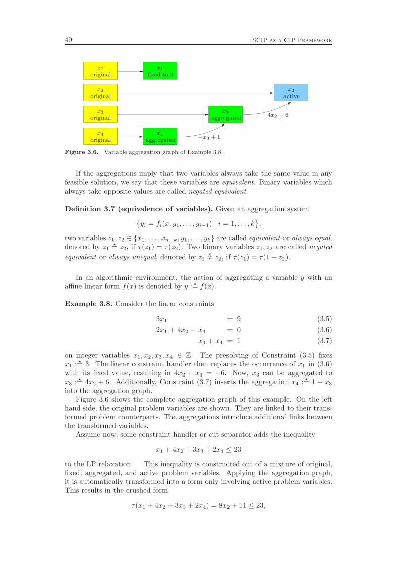
40 SCIP as a CIP Framework
x1x1
x2x2
x3x3
x4 x4−x3 + 1
4x2 + 6
original
original
original
original
aggregated
aggregated
active
fixed to 3
Figure 3.6. Variable aggregation graph of Example 3.8.
If the aggregations imply that two variables always take the same value in anyfeasible solution, we say that these variables are equivalent. Binary variables whichalways take opposite values are called negated equivalent.
Definition 3.7 (equivalence of variables). Given an aggregation system{yi = fi(x, y1, . . . , yi−1) | i = 1, . . . , k
},
two variables z1, z2 ∈ {x1, . . . , xn−k, y1, . . . , yk} are called equivalent or always equal,denoted by z1
⋆= z2, if τ(z1) = τ(z2). Two binary variables z1, z2 are called negated
equivalent or always unequal, denoted by z1 Y⋆= z2, if τ(z1) = τ(1− z2).
In an algorithmic environment, the action of aggregating a variable y with anaffine linear form f(x) is denoted by y : ⋆= f(x).
Example 3.8. Consider the linear constraints
3x1 = 9 (3.5)
2x1 + 4x2 − x3 = 0 (3.6)
x3 + x4 = 1 (3.7)
on integer variables x1, x2, x3, x4 ∈ Z. The presolving of Constraint (3.5) fixesx1 : ⋆= 3. The linear constraint handler then replaces the occurrence of x1 in (3.6)with its fixed value, resulting in 4x2 − x3 = −6. Now, x3 can be aggregated tox3 : ⋆= 4x2 + 6. Additionally, Constraint (3.7) inserts the aggregation x4 : ⋆= 1 − x3
into the aggregation graph.Figure 3.6 shows the complete aggregation graph of this example. On the left
hand side, the original problem variables are shown. They are linked to their trans-formed problem counterparts. The aggregations introduce additional links betweenthe transformed variables.
Assume now, some constraint handler or cut separator adds the inequality
x1 + 4x2 + 3x3 + 2x4 ≤ 23
to the LP relaxation. This inequality is constructed out of a mixture of original,fixed, aggregated, and active problem variables. Applying the aggregation graph,it is automatically transformed into a form only involving active problem variables.This results in the crushed form
τ(x1 + 4x2 + 3x3 + 2x4) = 8x2 + 11 ≤ 23,
3.3. Infrastructure 41
which is actually passed as 8x2 ≤ 12 to the LP solver. From this inequality, we canderive the bound change x2 ≤ 1, which also automatically produces the correspond-ing bound changes x3 ≤ 10 and x4 ≥ −9.
3.3.5 Implication Graph and Clique Table
Atamtürk, Nemhauser, and Savelsbergh [24] proposed the notion of a conflict graphto store assignment pairs (xi = vi, xj = vj) of binary variables xi, xj ∈ {0, 1} thatcannot occur in any feasible solution. Such conflicting assignments can be detectedin the presolving stage by constraint handlers or presolver plugins, in particular bythe probing presolver, see Section 10.6. The conflict graph G = (V,E) consists ofvertices V = {xj , xj | j = 1, . . . , n}, and edges E ⊆ {uv | u, v ∈ V, u = 1→ v = 0}.3
Note that this condition is symmetric and hence G is undirected. Each edge of thegraph represents one pair of conflicting variable assignments. The conflict graphdefines a stable set relaxation of the problem instance, since variable assignmentscan only occur in a feasible solution if the corresponding vertices are not adjacentin the graph. Atamtürk, Nemhauser, and Savelsbergh use this relaxation togenerate cutting planes which are known to be valid or facet defining for the stableset polytope, for example clique inequalities or odd-hole inequalities.
We take a slightly different approach. Instead of storing conflicting assignmentsin a conflict graph, we store implications in an implication graph. Additionally,we do not only store implications between binary variables, but also include impli-cations between binary and arbitrary variables. Note also, that we use the term“conflict graph” for a different object which is constructed during conflict analysis,see Chapter 11.
Definition 3.9 (implication graph). Let CIP = (C, I, c) be a CIP instance onvariables x ∈ Rn, xj ∈ Z for j ∈ I ⊆ N = {1, . . . , n}, and let B ⊆ I be the indices ofthe binary variables xj ∈ {0, 1}. Then, the implication graph for CIP is the directedinfinite graph D = (V,A) with vertices
V = {(xj ≤ v), (xj ≥ v) | j ∈ N, v ∈ R}
and arcs
A = {(xi ≤ 0, xj ≤ v) | i ∈ B, j ∈ N, v ∈ R, xi = 0→ xj ≤ v} ∪
{(xi ≤ 0, xj ≥ v) | i ∈ B, j ∈ N, v ∈ R, xi = 0→ xj ≥ v} ∪
{(xi ≥ 1, xj ≤ v) | i ∈ B, j ∈ N, v ∈ R, xi = 1→ xj ≤ v} ∪
{(xi ≥ 1, xj ≥ v) | i ∈ B, j ∈ N, v ∈ R, xi = 1→ xj ≥ v},
which represent the derivable implications xi = vi → xj ≤ vj or xi = vi → xj ≥ vj
with i ∈ B, j ∈ N , vi ∈ {0, 1}, vj ∈ R.
Since one usually does not know all implications between the variables, the graphstored during the solving process is in general only a partial version of the fullimplication graph. Furthermore, we store only those nodes and arcs that are needed
3In general, we can only construct a subset of all conflict edges, since generating the full conflictgraph is NP-hard: deciding the feasibility of a binary programming instance is NP-complete (seeGarey and Johnson [92]), and for a given binary programming instance the conflict graph is thecomplete graph if and only if the instance is infeasible.
42 SCIP as a CIP Framework
to represent the strongest implications for each binary variable assignment that areknown to the solver, i.e.,
xi = vi → xj ≤ min{vj | xi = vi → xj ≤ vj}
and
xi = vi → xj ≥ max{vj | xi = vi → xj ≥ vj}.
Note that due to Condition (1.1) of Definition 1.6, there are no implications on con-tinuous variables with strict inequalities in a constraint integer program. Therefore,the minimum and maximum above always exist or are infinite in which case thebinary variable can be fixed to the opposite value.
The implication graph includes all conflicting assignments between binary vari-ables. For such an assignment xi = 1 → xj = 0, both arcs (xi ≥ 1, xj ≤ 0) and(xj ≥ 1, xi ≤ 0) are member of the implication graph. Implications xi = vi → xj ≤vj or xi = vi → xj ≥ vj between binary variables xi and non-binary variables xj areonly included unidirectional. The other direction is implicitly stored as a variablebound of xj :
Definition 3.10 (variable bounds). Let xi, i ∈ I, be an integer variable and xj ,j ∈ N , be an arbitrary variable of a constraint integer program. Valid inequalities
xj ≥ sxi + d or xj ≤ sxi + d
with s, d ∈ R are called variable lower bounds and variable upper bounds of xj ,respectively.
Note that in the definition of the variable bounds, the variable xi does not need tobe binary. If xi is binary, however, the implications of xi are related to the variablebounds of xj .
Observation 3.11. Each implication on binary variables xi ∈ {0, 1} and arbitraryvariables xj ∈ [lj , uj ] gives rise to a variable bound of xj :
xi = 0→ xj ≤ vj ⇔ xj ≤ (uj − vj)xi + vj
xi = 0→ xj ≥ vj ⇔ xj ≥ (lj − vj)xi + vj
xi = 1→ xj ≤ vj ⇔ xj ≤ (vj − uj)xi + uj
xi = 1→ xj ≥ vj ⇔ xj ≥ (vj − lj)xi + lj
if the corresponding global bound lj or uj is finite.
SCIP stores the variable bounds in a similar data structure as the implications.This means, given a non-binary variable xj , we can find all implications with xj inthe conclusion by inspecting the list of variable bounds of xj . Whenever implicationsbetween binary variables are added, the arcs for both directions are added to theimplication graph. If an implication between a binary variable xi and a non-binaryvariable xj is added, a corresponding variable bound for xj is added to the variablebounds data structure. If a variable bound is added for xj with xi being binary,a corresponding implication between xi and xj is added to the implication graph.Furthermore, the implication graph is always maintained to be closed with respectto transitivity.
3.3. Infrastructure 43
For certain types of problem instances, in particular for set partitioning and setpacking instances, the explicit construction of the implication graph can consumehuge amounts of memory. For example, consider the set partitioning constraint
q∑
j=1
xj = 1
with xj ∈ {0, 1} for all j = 1, . . . , q. In this case, every fixing of xj = 1 leads toimplications xj = 1→ xk = 0 for all k 6= j. This means that each pair of variablesin the constraint yields an arc in the implication graph, and thus, the number ofarcs is quadratic in the number of variables. Typical set partitioning instanceshave a lot of variables, but only a few constraints. Take the instance nw04 fromMiplib 2003 [4, 6] as an example. It has 87482 variables, 36 constraints, and 636666non-zero coefficients, which gives an average of 17685 variables per constraint. Thisleads to about 11 billion implications, and with 20 bytes used for each implicationin SCIP’s data structures, this results in 220 gigabyte memory consumption.
To avoid this situation, such sets of pairwise contradicting assignments of binaryvariables are stored in a separate table. This table is called clique table, since thevariable assignments form a clique in the conflict graph as defined by Atamtürk,Nemhauser, and Savelsbergh [24]. We denote this table by Q and write Q(xj = v),v ∈ {0, 1}, to refer to the set of cliques the variable xj (v = 1) or its negation xj
(v = 0) is member of.In the example of nw04, we just have to store 36 cliques in the clique table, each
of them having 17685 members on average. Using 12 bytes per element in the clique,this yields a memory consumption of about 8 Megabyte. The small disadvantage ofthe clique table is that we now have to scan two different data structures when wewant to check for implications of a binary variable. In particular, this complicatesthe implementation of the clique cut separator, see Section 8.7.
3.3.6 Branching Tree
The subproblems that are processed during the branch-and-bound search are or-ganized as a branching tree, see Section 2.1. The root node of the tree representsthe global problem instance R. The partitioning of a problem Q into subproblemsQ1, . . . ,Qk by branching creates child nodes of Q. Except for the root node, eachnode Q has a unique parent node p(Q). Child nodes Qi, Qj with the same parentnode p(Qi) = p(Qj) are called siblings. The nodes on the path from the parent nodep(Qi) to the root node R are called ancestors of Q. If a subproblem is pruned (dueto bounding, infeasibility, or optimality), it is removed from the tree. Additionally,its ancestors are removed recursively as long as they have no other children. If theroot node is removed, the problem instance has been solved.
The search tree can be partitioned into depth levels, where the level d(Q) of anode Q is the length of the shortest path from Q to the root node R. This means,the root node is in depth level d(R) = 0, and the children Qi of a node Q are indepth level d(Qi) = d(Q) + 1.
SCIP stores the subproblem information using trailing, which means to only storethe differences to the parent node p(Q) in the subproblem Q. Therefore, to switchfrom one subproblem Q to the next subproblem Q′, one has to find the commonancestor Q of Q and Q′ of maximal depth, undo the problem changes on the pathfrom Q to Q, and apply the changes on the path from Q to Q′. An alternative totrailing is to employ copying where the whole problem information is stored at each
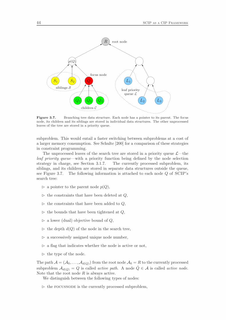
44 SCIP as a CIP Frameworkreplacemen
root node
focus node
siblings S
children C
leaf priorityqueue L
R
Q
Q1 Q2 Q3
S1 S2 L1
L2 L3
p(Q)
Figure 3.7. Branching tree data structure. Each node has a pointer to its parent. The focusnode, its children and its siblings are stored in individual data structures. The other unprocessedleaves of the tree are stored in a priority queue.
subproblem. This would entail a faster switching between subproblems at a cost ofa larger memory consumption. See Schulte [200] for a comparison of these strategiesin constraint programming.
The unprocessed leaves of the search tree are stored in a priority queue L—theleaf priority queue—with a priority function being defined by the node selectionstrategy in charge, see Section 3.1.7. The currently processed subproblem, itssiblings, and its children are stored in separate data structures outside the queue,see Figure 3.7. The following information is attached to each node Q of SCIP’ssearch tree:
⊲ a pointer to the parent node p(Q),
⊲ the constraints that have been deleted at Q,
⊲ the constraints that have been added to Q,
⊲ the bounds that have been tightened at Q,
⊲ a lower (dual) objective bound of Q,
⊲ the depth d(Q) of the node in the search tree,
⊲ a successively assigned unique node number,
⊲ a flag that indicates whether the node is active or not,
⊲ the type of the node.
The path A = (A0, . . . ,Ad(Q)) from the root nodeA0 = R to the currently processed
subproblem Ad(Q) = Q is called active path. A node Q ∈ A is called active node.Note that the root node R is always active.
We distinguish between the following types of nodes:
⊲ the focusnode is the currently processed subproblem,

3.3. Infrastructure 45
⊲ a sibling is a sibling of the focus node that was not yet stored in the leafpriority queue,
⊲ a child is a child of the focus node,
⊲ a leaf is a leaf which is stored in the leaf priority queue,
⊲ a junction is an already processed subproblem for which the LP relaxationwas not solved, and
⊲ a fork is an already processed subproblem for which the LP relaxation wassolved.
In fact, there are some more node types, namely probingnode, deadend, pseudo-fork, subroot, and refocusnode. We omit these additional node types in thepresentation, since they are only needed due to technical implementation issues.
Depending on the type of the node, additional node information is stored at asubproblem:
⊲ the number of existing children (focusnode, junction, fork),
⊲ the columns and rows that have been added to the LP relaxation (focusnode,fork),
⊲ the LP warm start information (focusnode, fork), and
⊲ a pointer to the fork parent, i.e., the ancestor of maximal depth for whichthe LP relaxation was solved (sibling, child, leaf).
The main operation that is supported by the branching tree is the switchingbetween subproblems Q and Q′, which is depicted in Algorithm 3.1. In order tofind the common ancestor Q of Q and Q′ in Step 1, we just have to follow the pathfrom Q′ to the root node R until an active node is discovered. Note that the loopalways terminates, since the root node is active. Step 2 restores the ancestor Q byundoing all problem and LP changes on the path from Q to Q in reverse direction.Since the problem and LP changes from Q to Q′ have to be applied in forwarddirection, and we can only traverse the tree in backward direction from the leaves tothe root, we have to first construct the new active path A in Step 3. Afterwards, thepath can be traversed in the desired direction in order to apply the problem changesand to construct subproblem Q′.
If the old focus node Q has children, i.e., a branching took place to solve thesubproblem, it is converted into a fork or junction node in Step 5. If the LPrelaxation was solved, the current warm start information is retrieved from the LPsolver, and the node type is set to fork. If the LP relaxation of Q was not solvedor if it was discarded due to numerical difficulties, the node type is set to junction.
If the old focus node has no children, it is either infeasible, exceeds the primalbound, or was solved to optimality. In any case, it can be pruned from the tree,thereby reducing the number of live children of its parent p(Q). If the parent nowalso has no more children, it can be deleted as well, and the deletion can be continuedrecursively.
Steps 6 to 8 update the sets of current siblings S, children C, and active leaves L.If the new focus node Q′ is a child of the old focus node Q, the former children
become siblings and the former siblings are moved to the leaf priority queue. IfQ′ is a sibling of Q, the other siblings remain siblings, and the former children are

46 SCIP as a CIP Framework
Algorithm 3.1 Node Switching
Input : current subproblem Q with siblings S = {S1, . . . , Sl} and children C ={Q1, . . . ,Qk}, active path A, and leaf priority queue L; next subproblemQ′ to be processed which is of type sibling, or child, or which is thetop-priority leaf in L.
Output : updated data structures such that the new current problem is Q′.
1. Find the common ancestor node Q of Q and Q′ of maximal depth:
(a) Set Q := Q′.
(b) While Q is not active, set Q := p(Q).
2. Undo all problem and LP changes on the path from Q to Q:
(a) Set Q := Q.
(b) While Q 6= Q:
i. Remove the columns and rows from the LP relaxation that have beenadded at Q.
ii. Add the constraints that have been deleted from Q.iii. Delete the constraints that have been added to Q.iv. Relax the bounds that have been tightened at Q.v. Set Q := p(Q).
3. Update the active path:
(a) Set Q := Q′.
(b) While Q 6= Q: Set Ad(Q) := Q, and set Q := p(Q).
4. Apply all problem changes on the path from Q to Q′:
(a) For Q = Ad(Q), . . . ,Ad(Q′):
i. Tighten the bounds that have been tightened at Q.ii. Add the constraints that have been added to Q.iii. Delete the constraints that have been deleted from Q.iv. Add the columns and rows from the LP relaxation that have been
added at Q.
5. If C 6= ∅, convert Q into a fork or junction node, depending on whetherthe LP relaxation has been solved or not. Otherwise, delete Q and all of itsancestors without live children.
6. If Q′ is of type child: Convert siblings S to type leaf, set L := L∪S, convertchildren C \ {Q′} to type sibling, and set S := C \ {Q′} and C := ∅.
7. If Q′ is of type sibling: Convert children C to type leaf, and set L := L∪C,S := S \ {Q′}, and C := ∅.
8. If Q′ is of type leaf: Convert siblings S and children C to type leaf, and setL := (L \ {Q′}) ∪ S ∪ C, S := ∅, and C := ∅.
9. Convert Q′ to type focusnode, and update Q := Q′.
10. Load the LP warm start information of the fork parent of Q.
3.3. Infrastructure 47
moved to the leaf priority queue. If the new focus node Q′ is a leaf from the priorityqueue, it is not a direct relative of the former children and siblings. Therefore, bothchildren and siblings must be moved to the leaf priority queue.
Step 9 installs node Q′ as the new focus node Q. Finally in Step 10, the LPwarm start information for the new focus node Q is loaded into the LP solver. Forsimplex solvers, this is usually the optimal simplex basis of the fork parent, butsince the warm start information is an abstract data type, which is implementedin the LP solver interface, each LP solver can store a different type of warm startinformation in the tree.
Note. The LP warm start information should be as compact as possible, since thewarm start information of a subproblem Q must stay in memory as long as thereis any active node left whose fork parent is Q. A simplex basis can be storedusing only two bits per row and column, since for each row (i.e., slack variable) andeach column we only need to know whether it is basic, on its lower, or on its upperbound. Using this information, the corresponding basic solution can be recalculatedby refactorizing the basis matrix and solving the corresponding equation systems.
Of course, it would improve the LP solving performance if we also stored thebasis matrix factorization, since this would save the effort for recalculating the initialfactorization. Unfortunately, the factorization usually consumes too much memoryto store it in the search tree for every node. A reasonable tradeoff is to apply depthfirst search or plunging node selection strategies, see Section 3.1.7 and Chapter 6.They tend to choose children of the current node as the next subproblem to beprocessed, which means that the current factorization which is still loaded in the LPsolver can be used further and does not need to be recalculated.
3.3.7 LP Relaxation
The LP relaxation stores a linear relaxation of the current subproblem. Like thestable set relaxation, given by the implication graph described in Section 3.3.5, itprovides a global view on the problem and a way of sharing information betweendifferent plugins.
We make the following notational distinctions between the CIP and its LP re-laxation. The CIP consists of variables and constraints. The variables are markedto be integer or continuous. The constraints are stored in constraint handler specificdata structures. Their semantics is unknown to the framework and only implicitlygiven by the actions performed in the constraint handlers’ callback methods. TheLP relaxation consists of columns and rows. For each column, the lower and upperbounds are known. Every column belongs to exactly one CIP variable, but not everyCIP variable needs to be represented by a column in the LP. The rows are definedas linear combinations of columns and have left and right hand sides as additionaldata. A single constraint like the TSP’s nosubtour constraint (see Example 3.2on page 24) can give rise to multiple rows in the LP, but rows can also live on theirown, e.g., if they were created by a general purpose cut separator.
The LP relaxation is created and extended by variable pricing and cutting planeseparation. Pricing of existing problem variables is performed automatically, whileunknown variables have to be treated by problem specific variable pricer plugins,see Section 3.1.5. New columns enter the LP through the pricing storage describedin Section 3.3.9. Cutting plane separation is performed by constraint handlers andseparators, see Sections 3.1.1 and 3.1.3, respectively. These linear inequalities and
48 SCIP as a CIP Framework
equations are passed to the LP relaxation via the separation storage explained inSection 3.3.8. Both variables and constraints can be marked to be initial whichmeans that their corresponding columns and rows form the initial LP of the rootnode relaxation. Afterwards, further extensions are applied in the price-and-cut loopduring the processing of the subproblems, see Section 3.2.8. The LP relaxation isautomatically updated during the switching between subproblems in the search tree,see Section 3.3.6.
For any given subproblem, the user may choose whether the LP relaxation shouldbe solved. By completely deactivating the LP relaxation, one can mimic a pureconstraint programming or SAT solver, while solving the LP relaxation at everynode is common for mixed integer programming solvers.
3.3.8 Separation Storage
Cutting planes are produced by constraint handlers and cut separators, see Sec-tions 3.1.1 and 3.1.3, respectively. After adding cuts, the LP is resolved, and theseparators are called again with the new LP solution. It turns out to be very ineffi-cient to immediately resolve the LP after the first cutting plane was found. Instead,one performs cutting plane separation in rounds. In each round, various cuttingplanes are generated to cut off the current LP solution. Since one does not wantto increase the size of the LP too much by adding all cutting planes that one canfind, they are first collected in the separation storage from which only a subset ofthe available cutting planes is selected to enter the LP.
The selection of the cuts to be added to the LP is a crucial decision which affectsthe performance and the stability of the LP solving process in the subsequent calls.In SCIP, the cuts are selected with respect to three different criteria:
⊲ the efficacy of the cuts, i.e., the distance of their corresponding hyperplanesto the current LP solution,
⊲ the orthogonality of the cuts with respect to each other, and
⊲ the parallelism of the cuts with respect to the objective function.
The first two have already been used by Balas, Ceria, and Cornuéjols [30] in thecontext of lift-and-project cuts, and by Andreello, Caprara, and Fischetti [13] for{0, 1
2}-cuts.It is tried to select a nearly orthogonal subset of cutting planes, which cut as deep
as possible into the current LP polyhedron. Cutting planes are slightly preferredif they are closer to being parallel to the objective function. The user has thepossibility to change the employed distance norm to measure the efficacy of thecuts. The default settings apply the Euclidean norm. The user can also adjust theimportance of the three criteria with respect to each other. Computational resultsto evaluate the cutting plane selection can be found in Section 8.10.
Algorithm 3.2 shows the details of the selection procedure. For each cut r ∈ Rthat was found in the current separation round, we calculate the efficacy er andthe objective function parallelism pr in Step 1. Using an initial orthogonality valueof or = 1, the initial score sr = s(er, pr, or) is computed. The score functions : R3 → R in SCIP combines the individual quality measures to produce a singlevalue by calculating a weighted sum s(er, pr, or) = weer +wppr +woor of the threeoperands with non-negative weights we, wp, wo ∈ R≥0. The weights themselves canbe adjusted by the user. The default settings are we = 1, wp = 0.1, and wo = 1.
3.3. Infrastructure 49
Algorithm 3.2 Cutting Plane Selection
Input : current LP solution x and set R of generated cutting planes; a score func-tion s : R3 → R, the minimal orthogonality minortho ∈ [0, 1], and themaximal number maxsepacuts of separated cuts per round.
Output : updated LP relaxation.
1. For all r ∈ R with r : γr ≤ dT
r x ≤ γr calculate:
(a) the efficacy er := max{γr − dT
r x, dT
r x− γr}/‖dr‖,
(b) the objective parallelism pr := |dT
r c| / (‖dr‖ · ‖c‖),
(c) the initial orthogonality or := 1, and
(d) the initial score sr := s(er, pr, or).
2. While R 6= ∅ and less than maxsepacuts cuts have been added to the LP:
(a) Add cut r⋆ ∈ R with largest score sr⋆ to the LP. Set R := R \ {r⋆}.
(b) For all cuts r ∈ R:
i. Update or := min{or, 1 − |d
T
r⋆dr| / (‖dr⋆‖ · ‖dr‖)}
.ii. If or < minortho, set R := R \ {r}.
Otherwise, update sr := s(er, pr, or).
After calculating the initial score values, the cuts are consecutively passed tothe LP relaxations in Loop 2 until the cut list is empty or a maximum numbermaxsepacuts of cuts has been added. In each iteration of the loop, a cut r⋆ withlargest score sr⋆ is selected in Step 2a and enters the LP. Afterwards, we updatethe orthogonalities or of the remaining cuts r ∈ R in Step 2b. A cut is discardedif its orthogonality falls below the threshold minortho. Otherwise, we recalculate itsscore sr.
SCIP uses a default setting of minortho = 0.5. The number of cuts generated perround is restricted to maxsepacuts = 2000 in the root node and to maxsepacuts =100 in subproblems. Using a minimal orthogonality minortho > 0 automaticallyremoves all cuts that are dominated by or are equal to parallel cuts. Strongerdomination criteria that take the current bounds of the variables into account arenot applied. However, cuts can be marked to be “removable”, which means that theywill be eliminated from the LP if they are not satisfied with equality for a numberof separation rounds or in the final LP solution. Thereby, dominated “removable”cuts are automatically deleted from the LP relaxation with a slight delay.
The results of computational experiments to evaluate various cut selection poli-cies can be found in Section 8.10 in the context of cutting plane separation for mixedinteger programs.
3.3.9 Pricing Storage
Like cutting plane separation, pricing of variables is performed in rounds. In everypricing round, the current problem variables which are not yet represented in the LPare inspected to check whether their inclusion in the LP relaxation would potentiallydecrease (i.e., improve) the LP objective value. Additionally, all activated pricerplugins are called to generate new variables. These candidate variables for enteringthe LP as columns are collected in a pricing storage.
In contrast to cutting planes, the CIP framework does not have enough informa-
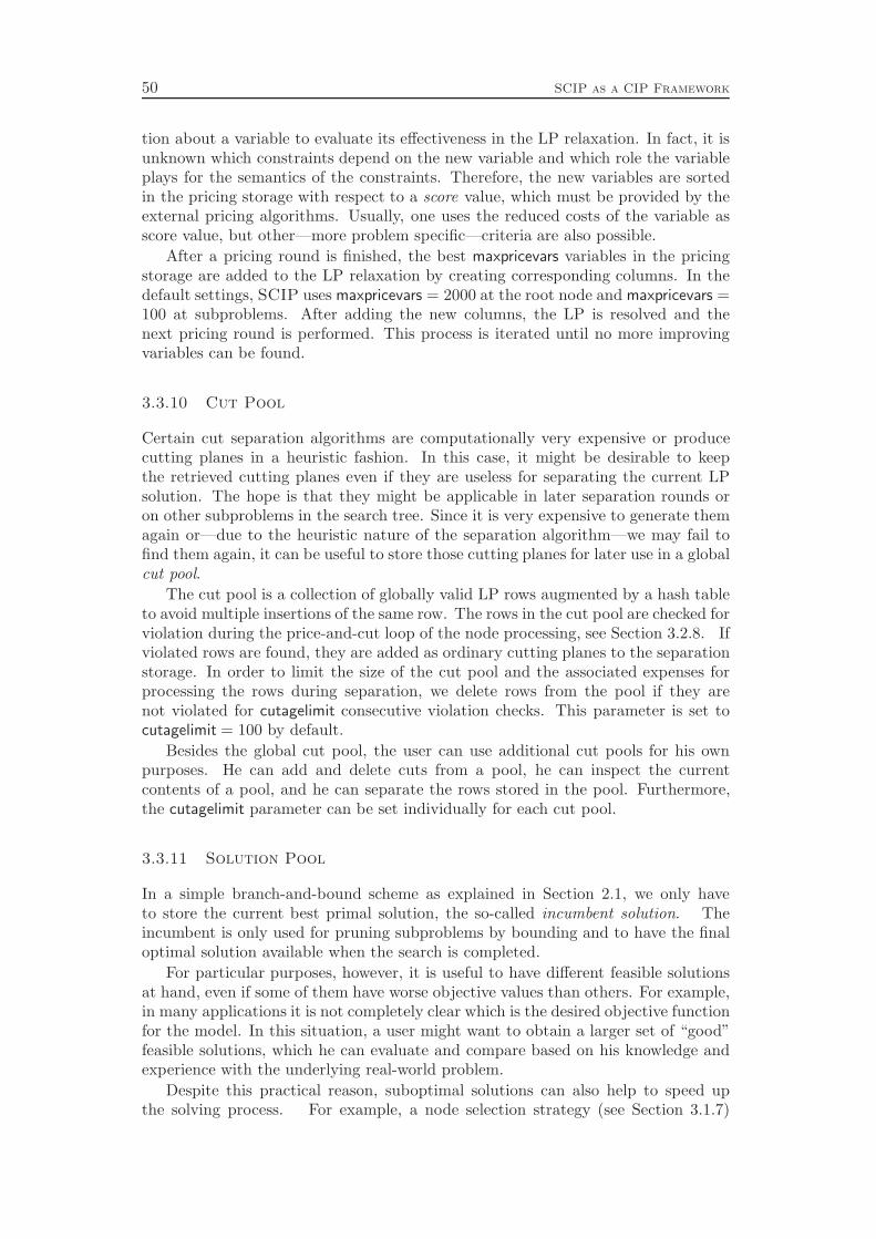
50 SCIP as a CIP Framework
tion about a variable to evaluate its effectiveness in the LP relaxation. In fact, it isunknown which constraints depend on the new variable and which role the variableplays for the semantics of the constraints. Therefore, the new variables are sortedin the pricing storage with respect to a score value, which must be provided by theexternal pricing algorithms. Usually, one uses the reduced costs of the variable asscore value, but other—more problem specific—criteria are also possible.
After a pricing round is finished, the best maxpricevars variables in the pricingstorage are added to the LP relaxation by creating corresponding columns. In thedefault settings, SCIP uses maxpricevars = 2000 at the root node and maxpricevars =100 at subproblems. After adding the new columns, the LP is resolved and thenext pricing round is performed. This process is iterated until no more improvingvariables can be found.
3.3.10 Cut Pool
Certain cut separation algorithms are computationally very expensive or producecutting planes in a heuristic fashion. In this case, it might be desirable to keepthe retrieved cutting planes even if they are useless for separating the current LPsolution. The hope is that they might be applicable in later separation rounds oron other subproblems in the search tree. Since it is very expensive to generate themagain or—due to the heuristic nature of the separation algorithm—we may fail tofind them again, it can be useful to store those cutting planes for later use in a globalcut pool.
The cut pool is a collection of globally valid LP rows augmented by a hash tableto avoid multiple insertions of the same row. The rows in the cut pool are checked forviolation during the price-and-cut loop of the node processing, see Section 3.2.8. Ifviolated rows are found, they are added as ordinary cutting planes to the separationstorage. In order to limit the size of the cut pool and the associated expenses forprocessing the rows during separation, we delete rows from the pool if they arenot violated for cutagelimit consecutive violation checks. This parameter is set tocutagelimit = 100 by default.
Besides the global cut pool, the user can use additional cut pools for his ownpurposes. He can add and delete cuts from a pool, he can inspect the currentcontents of a pool, and he can separate the rows stored in the pool. Furthermore,the cutagelimit parameter can be set individually for each cut pool.
3.3.11 Solution Pool
In a simple branch-and-bound scheme as explained in Section 2.1, we only haveto store the current best primal solution, the so-called incumbent solution. Theincumbent is only used for pruning subproblems by bounding and to have the finaloptimal solution available when the search is completed.
For particular purposes, however, it is useful to have different feasible solutionsat hand, even if some of them have worse objective values than others. For example,in many applications it is not completely clear which is the desired objective functionfor the model. In this situation, a user might want to obtain a larger set of “good”feasible solutions, which he can evaluate and compare based on his knowledge andexperience with the underlying real-world problem.
Despite this practical reason, suboptimal solutions can also help to speed upthe solving process. For example, a node selection strategy (see Section 3.1.7)

3.3. Infrastructure 51
might want to consider regions of the search tree first, that are close to a number offeasible solutions. The hope is to find more and even better solutions in this region.A branching rule (see Section 3.1.6) might want to branch on variables first that areset to the same value in all feasible solutions found so far. If the subproblem becomesinfeasible in the opposite branching direction, the variable can be fixed. The mostimportant benefits of a large pool of different feasible solutions, however, are primalheuristics, see Section 3.1.8 and Chapter 9. In particular the improvement heuristicsconsider also suboptimal solutions as a starting point from which improved solutionscan be found.
SCIP stores the best maxsol solutions with respect to the objective value in asorted array which is called the solution pool. The first element of this array is theincumbent solution. In the default settings, the size of the solution pool is restrictedto maxsol = 100.
3.3.12 Memory Management
The internal memory management of SCIP provides three different memory alloca-tion techniques:
⊲ standard memory management,
⊲ block memory management, and
⊲ memory buffers.
Depending on the type of data object and its life cycle, one of the three techniquesshould be selected to allocate the necessary memory.
Standard Memory Management
Standard memory management denotes the allocation and deallocation of memorywith the standard methods malloc() and free() of the C programming language.In fact, in optimized compilation mode, SCIP’s methods for standard memory man-agement are only synonyms for these C methods. In debugging mode, however, stan-dard memory management includes the maintenance of a list of currently allocatedmemory regions together with the source code lines at which each memory regionwas allocated. At the end of the program execution the list contains the memoryregions that were not deallocated and can therefore detect memory leaks.
Block Memory Management
During a typical run of SCIP to solve a CIP instance, many data objects of the sametype are allocated and deallocated from the memory heap of the system process. Forexample, there may exist thousands of cutting plane data structures or millions ofbranch-and-bound nodes. Using the standard malloc() and free() methods canlead to a substantial overhead caused by the free list management of this allocatorand the operating system.
A common way of improving runtime performance in memory management is toreplace the standard memory allocator with a program specific allocation method. Athorough review of allocator strategies can be found in Wilson et al. [215]. The blockmemory management of SCIP implements a suballocator (see [191]) using a segre-gated free lists scheme with exact lists (see Comfort [67]). For each memory block

52 SCIP as a CIP Framework
1
10
100
1000
10000
100000
1000000
10000000
4 16 64 256 1024 4096 16384 65536
arki001
block size
nu
mb
erof
blo
cks
1
10
100
1000
10000
100000
1000000
10000000
2 4 8 16 32 64 128 256 512 1024
markshare1
block size
nu
mb
erof
blo
cks
Figure 3.8. Histograms of block sizes allocated after processing 1 000 000 branch-and-bound nodesof the MIP instances arki001 and markshare1.
size, a single-linked list of free memory blocks is maintained. The lists themselvesare stored in a hash map referenced by the block size. If a memory block of a certainsize is allocated, the first element in the corresponding free list is unlinked from thelist and returned to the user. If the free list is empty, a new chunk of memory isallocated by calling malloc(). The chunk is split into blocks of the correspondingsize, which are added to the free list. The sizes of the chunks grow exponentiallywith the number of chunks allocated for a given block size. Thereby, the number ofmalloc() calls is logarithmic in the maximal number of simultaneously live blocks.
If a memory block is no longer needed, the user has to call the deallocationmethod of the block memory allocator, which has to add the block to the free listof the corresponding block size. Therefore, the allocator has to know the size ofthe freed block. Many existing memory allocators for C replace the malloc() andfree() calls by own implementations. This has the advantage that the user doesnot need to modify the source code. Since free() does not provide the size ofthe freed memory block as a parameter, the allocator has to retrieve the size bydifferent means. Usually, the size of a block is recorded in a header field, which isan additional word located in front of the actual data block. This means, that thememory consumption is increased by one word per memory block.
Figure 3.8 shows typical memory allocation histograms as they appear during thesolving process of MIP instances. Note that both axes are logarithmically scaled.The instance arki001 is a medium sized MIP with 1388 variables and 1048 con-straints. One can see that most memory blocks are of small size: 78 % of theallocated blocks are smaller or equal than 44 bytes, which is the size of the branch-and-bound node data structure in SCIP on a 32-bit processor. The average blocksize is 101.3 bytes. For the very small instance markshare1 with 62 variables and 6constraints, the allocation histogram shows an even larger tendency towards small
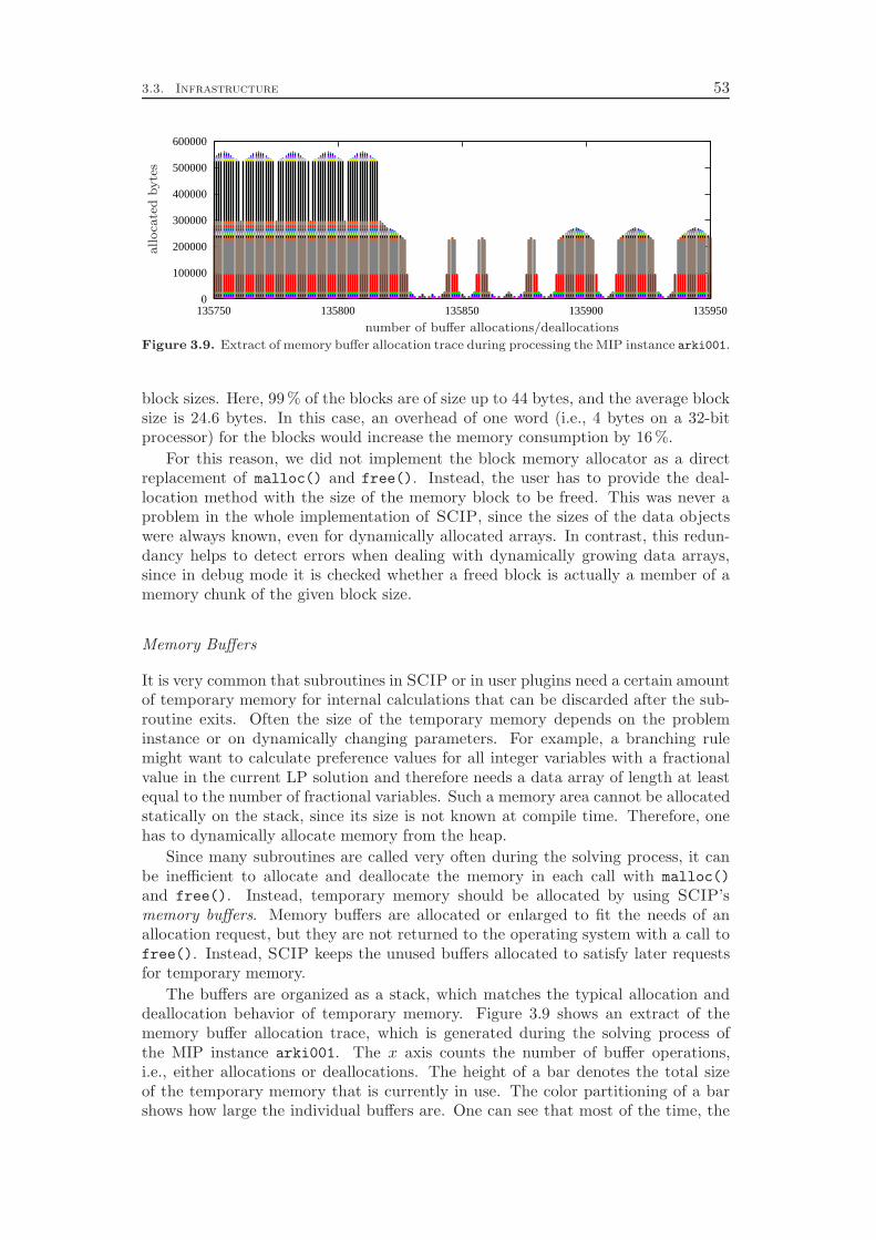
3.3. Infrastructure 53
0
100000
200000
300000
400000
500000
600000
135750 135800 135850 135900 135950
number of buffer allocations/deallocations
all
oca
ted
by
tes
Figure 3.9. Extract of memory buffer allocation trace during processing the MIP instance arki001.
block sizes. Here, 99 % of the blocks are of size up to 44 bytes, and the average blocksize is 24.6 bytes. In this case, an overhead of one word (i.e., 4 bytes on a 32-bitprocessor) for the blocks would increase the memory consumption by 16 %.
For this reason, we did not implement the block memory allocator as a directreplacement of malloc() and free(). Instead, the user has to provide the deal-location method with the size of the memory block to be freed. This was never aproblem in the whole implementation of SCIP, since the sizes of the data objectswere always known, even for dynamically allocated arrays. In contrast, this redun-dancy helps to detect errors when dealing with dynamically growing data arrays,since in debug mode it is checked whether a freed block is actually a member of amemory chunk of the given block size.
Memory Buffers
It is very common that subroutines in SCIP or in user plugins need a certain amountof temporary memory for internal calculations that can be discarded after the sub-routine exits. Often the size of the temporary memory depends on the probleminstance or on dynamically changing parameters. For example, a branching rulemight want to calculate preference values for all integer variables with a fractionalvalue in the current LP solution and therefore needs a data array of length at leastequal to the number of fractional variables. Such a memory area cannot be allocatedstatically on the stack, since its size is not known at compile time. Therefore, onehas to dynamically allocate memory from the heap.
Since many subroutines are called very often during the solving process, it canbe inefficient to allocate and deallocate the memory in each call with malloc()
and free(). Instead, temporary memory should be allocated by using SCIP’smemory buffers. Memory buffers are allocated or enlarged to fit the needs of anallocation request, but they are not returned to the operating system with a call tofree(). Instead, SCIP keeps the unused buffers allocated to satisfy later requestsfor temporary memory.
The buffers are organized as a stack, which matches the typical allocation anddeallocation behavior of temporary memory. Figure 3.9 shows an extract of thememory buffer allocation trace, which is generated during the solving process ofthe MIP instance arki001. The x axis counts the number of buffer operations,i.e., either allocations or deallocations. The height of a bar denotes the total sizeof the temporary memory that is currently in use. The color partitioning of a barshows how large the individual buffers are. One can see that most of the time, the
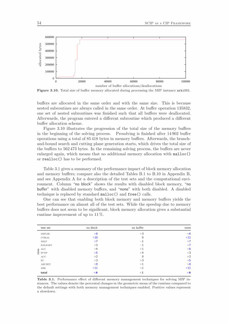
54 SCIP as a CIP Framework
0
100000
200000
300000
400000
500000
600000
0 20000 40000 60000 80000 100000
number of buffer allocations/deallocations
all
oca
ted
by
tes
Figure 3.10. Total size of buffer memory allocated during processing the MIP instance arki001.
buffers are allocated in the same order and with the same size. This is becausenested subroutines are always called in the same order. At buffer operation 135832,one set of nested subroutines was finished such that all buffers were deallocated.Afterwards, the program entered a different subroutine which produced a differentbuffer allocation scheme.
Figure 3.10 illustrates the progression of the total size of the memory buffersin the beginning of the solving process. Presolving is finished after 14 902 bufferoperations using a total of 85 418 bytes in memory buffers. Afterwards, the branch-and-bound search and cutting plane generation starts, which drives the total size ofthe buffers to 562 473 bytes. In the remaining solving process, the buffers are neverenlarged again, which means that no additional memory allocation with malloc()
or realloc() has to be performed.
Table 3.1 gives a summary of the performance impact of block memory allocationand memory buffers; compare also the detailed Tables B.1 to B.10 in Appendix B,and see Appendix A for a description of the test sets and the computational envi-ronment. Column “no block” shows the results with disabled block memory, “nobuffer” with disabled memory buffers, and “none” with both disabled. A disabledtechnique is replaced by standard malloc() and free() calls.
One can see that enabling both block memory and memory buffers yields thebest performance on almost all of the test sets. While the speedup due to memorybuffers does not seem to be significant, block memory allocation gives a substantialruntime improvement of up to 11 %.
test set no block no buffer none
tim
e
miplib +8 +3 +6
coral +10 0 +11
milp +7 −1 +7
enlight +3 −1 +7
alu +4 +1 +6
fctp +5 +4 +3
acc +2 0 +2
fc +3 +3 +5
arcset +9 +1 +8
mik +11 +1 +11
total +8 +1 +8
Table 3.1. Performance effect of different memory management techniques for solving MIP in-stances. The values denote the percental changes in the geometric mean of the runtime compared tothe default settings with both memory management techniques enabled. Positive values representa slowdown.

3.3. Infrastructure 55
Two interesting cases are the enlight and alu testsets, in which most instancesare quite small in size but require many branching nodes to solve. Thus, a com-parably large fraction of the time is spent on memory operations. One can seethat disabling block memory allocation yields a small slowdown of 3 % and 4 %,respectively, on these two test sets, but disabling memory buffers does not makeany significant difference. The comparison of columns “no block” and “none” shows,however, that with block memory turned off, memory buffers do have an impacton the performance. A possible explanation might be that with block memory, thebuffer memory allocations are almost the only remaining memory operations left,and that the standard allocator of malloc() and free() behaves very similar tothe memory buffer strategy. Without using block memory, temporary and long-termmemory allocations with malloc() are interleaved, which might negatively influencethe performance of the standard allocator.


Part II
Mixed Integer Programming
57

Chapter 4
Introduction
Integer programming and mixed integer programming emerged in the late 1950’s andearly 1960’s when researchers realized that the ability to solve mixed integer pro-gramming models would have great impact for practical applications (see Markowitzand Manne [156] and Dantzig [74]). Gomory [104] and Martin [161] discovered thefirst algorithms that can solve integer programs to optimality in a finite numberof steps. Further details on the history of integer programming can be found inGomory [105].
Mixed integer programming has applications in a large variety of domains, in-cluding scheduling, project planning, public transport, air transport, telecommuni-cations, economics and finance, timetabling, mining, and forestry. Many of theseexamples can be found in Heipcke [114].
As there is a lot of commercial interest in solving MIPs, it is not surprising thatthe development of MIP solvers soon became itself a commercial endeavor. Today’sbest tools for mixed integer programming are developed by commercial vendors,including Cplex [118], Lingo [148], and Xpress [76]. The source code of thesesolvers is proprietary, which imposes some difficulties for academic researchers toevaluate new ideas by computations within a state-of-the-art environment. Despiteits integration of CP and SAT techniques into MIP solving, the development ofSCIP can be seen as an attempt to provide the MIP research community with afreely available software, which is (almost) comparable to the current commercialcodes in terms of performance. A benchmark comparison of Cplex and SCIP canbe found in Appendix C.
In this part of the thesis we investigate the key ingredients of branch-and-boundbased MIP solvers, discuss a number of different approaches and algorithms for eachcomponent, and present some new ideas. Chapter 5 evaluates different branchingrules and subsumes a number of well-known strategies under a new and very generalparameterized rule, the reliability branching rule. Chapter 6 presents and comparesdifferent strategies to select the next subproblem from the search tree to be processed.The selected node is then subject to the domain propagation algorithms, which arediscussed in Chapter 7. A very brief overview of various cutting plane separationalgorithms to strengthen the LP relaxation of the node is given in Chapter 8.
During the node solving process, primal heuristics are called at different pointsin order to generate feasible MIP solutions. A huge amount of proposals for MIPheuristics can be found in the literature. Chapter 9 presents the ones that are im-plemented in SCIP. Chapter 10 explains the presolving techniques that are usedto simplify the problem instance and to extract additional information about theinstance before the actual solving process commences. Finally, Chapter 11 gener-alizes the idea of conflict analysis in SAT solvers to mixed integer programming.Besides its value for mixed integer programming, we will see in Part III of the thesisthat conflict analysis is a very important tool for solving the chip design verificationproblem by constraint integer programming.
59
60 Introduction
Each chapter presents computational results to compare the effectiveness of thediscussed algorithms and strategies. The test set of MIP instances that we used andthe computational environment in which the experiments have been performed aredescribed in Appendix A.
We conclude this introduction by recapitulating the basic definitions of mixedinteger programming as they have been introduced in Section 1.3.
A mixed integer program (MIP) is defined as follows.
Definition (mixed integer program). Given a matrix A ∈ Rm×n, vectors b ∈Rm, and c ∈ Rn, and a subset I ⊆ N = {1, . . . , n}, the mixed integer programMIP = (A, b, c, I) is to solve
(MIP) c⋆ = min {cTx | Ax ≤ b, x ∈ Rn, xj ∈ Z for all j ∈ I} .
The vectors in the set XMIP = {x ∈ Rn | Ax ≤ b, xj ∈ Z for all j ∈ I} are calledfeasible solutions of MIP. A feasible solution x⋆ ∈ XMIP of MIP is called optimal ifits objective value satisfies cTx⋆ = c⋆.
The bounds of the variables are denoted by lj ≤ xj ≤ uj with lj , uj ∈ R∪{±∞}.Formally, they are part of the constraint system Ax ≤ b, but in practice they aretreated outside the coefficient matrix. Depending on the integrality status andthe bounds of the variables, we define the following subsets of the variable indicesN = {1, . . . , n}:
binary variables: B := {j ∈ I | lj = 0 and uj = 1}
integer variables: I
continuous variables: C := N \ I
Specializations of MIPs are
⊲ linear programs (LPs) with I = ∅,
⊲ integer programs (IPs) with I = N ,
⊲ mixed binary programs (MBPs) with B = I, and
⊲ binary programs (BPs) with B = I = N .
If we remove the integrality restrictions from an MIP, we obtain its LP relaxation:
Definition (LP relaxation of an MIP). Given a mixed integer program MIP =(A, b, c, I), its LP relaxation is defined as
(LP) c = min {cTx | Ax ≤ b, x ∈ Rn} .
XLP = {x ∈ Rn | Ax ≤ b} is the set of feasible solutions of the LP relaxation. AnLP-feasible solution x ∈ XLP is called LP-optimal if cT x = c.
The solution set of the LP relaxation defines a polyhedron P = XLP. This LPpolyhedron is a superset of its integer hull PI ⊆ P , which is the convex hull
PI = conv{P ∩ (ZI × RN\I)} = conv{XMIP}
of the MIP feasible solutions.
Chapter 5
Branching
Most of this chapter is joint work with Thorsten Koch and Alexander Martin. Partsof it were published in Achterberg, Koch, and Martin [5].
Since branching is in the core of any branch-and-bound algorithm, finding goodstrategies was important to practical MIP solving right from the beginning, see Béni-chou et al. [39] or Mitra [165]. We refrain from giving details of all existing strategies,but concentrate on the most popular rules used in todays MIP solvers, in particularthe ones that are available in SCIP. For a comprehensive study of branch-and-boundstrategies we refer to Land and Powell [139], Linderoth and Savelsbergh [146], Fü-genschuh and Martin [90], and the references therein.
The only way to split a problem Q within an LP based branch-and-bound al-gorithm is to branch on linear inequalities in order to keep the property of havingan LP relaxation at hand. The easiest and most common inequalities are trivialinequalities, i.e., inequalities that split the feasible interval of a singleton variable,compare Figure 2.2 on page 17. To be more precise, if xj , j ∈ I, is some integervariable with a fractional value xj in the current optimal LP solution, we obtaintwo subproblems: one by adding the trivial inequality xj ≤ ⌊xj⌋ (called the leftsubproblem or left child, denoted by Q−j ) and one by adding the trivial inequality
xj ≥ ⌈xj⌉ (called the right subproblem or right child, denoted by Q+j ). This proce-
dure of branching on trivial inequalities is also called branching on variables, becauseit only requires to change the bounds of variable xj . Branching on more compli-cated inequalities or even splitting the problem into more than two subproblemsare rarely incorporated into general MIP solvers, even though it can be effectivein special cases, see, for instance, Borndörfer, Ferreira, and Martin [51], Clochardand Naddef [62], or Naddef [169]. SCIP supports general branching on constraintswith an arbitrary number of children, but all of the branching rules included in thedistribution branch on variables and create a binary search tree.
The basic algorithm for variable selection may be stated as follows:
Algorithm 5.1 Generic variable selection
Input : Current subproblem Q with an optimal LP solution x /∈ XMIP.
Output : An index j ∈ I of an integer variable xj with fractional LP value xj /∈ Z.
1. Let F = {j ∈ I | xj /∈ Z} be the set of branching candidates.
2. For all candidates j ∈ F , calculate a score value sj ∈ R.
3. Return an index j ∈ F with sj = maxk∈F{sk}.
In the following we focus on the most common variable selection rules, which areall variants of Algorithm 5.1. The difference is how the score in Step 2 is computed.
The ultimate goal is to find a computationally inexpensive branching strategythat minimizes the number of branch-and-bound nodes that need to be evaluated.
61
62 Branching
Since no global approach is known, one tries to find a branching variable that is atleast a good choice for the current branching. One way to measure the quality ofa branching is to look at the changes in the objective function of the LP relaxationsof the two children Q−i and Q+
i compared to the relaxation of the parent node Q.Recently, Patel and Chinneck [185] proposed to favor branchings that result in LPsolutions xQ
−j
and xQ+
jwith a large Euclidean distance to the current LP solution
xQ. However, we follow the traditional way of trying to improve the dual bound.
In order to compare branching candidates, for each candidate the two objectivefunction changes ∆−j := cQ−
j− cQ and ∆+
j := cQ+
j− cQ or estimates of these values
are mapped on a single score value. This is typically done by using a function of theform
score(q−, q+) = (1− µ) ·min{q−, q+}+ µ ·max{q−, q+}, (5.1)
see, for instance, Linderoth and Savelsbergh [146]. The score factor µ is somenumber between 0 and 1. It is usually an empirically determined constant, which issometimes adjusted dynamically through the course of the algorithm (in SCIP weuse a static value of µ = 1
6, which is also used in SIP [159]). In addition, SCIP
features a new idea which is to calculate the score via a product
score(q−, q+) = max{q−, ǫ} ·max{q+, ǫ} (5.2)
with ǫ = 10−6. This product is the default score function in SCIP, and the com-putational results in Section 5.11 show its superiority to the weighted sum of Equa-tion (5.1). Bounding the values by ǫ is necessary to be able to compare two pairs(∆−j ,∆
+j ) and (∆−k ,∆
+k ) where one of the values is zero for each pair. There are
a lot of MIP instances where such a behavior can be observed, typically for thedownwards changes ∆−.
In the forthcoming explanations all cases are symmetric for the left and rightsubproblem. Therefore we will only consider one direction most of the time, theother will be analogous.
5.1 Most Infeasible Branching
This still very common rule chooses the variable with fractional part closest to 0.5,i.e., sj = φ(xj) = min{xj −⌊xj⌋, ⌈xj⌉− xj}. The heuristic reason behind this choiceis that this selects a variable where the least tendency can be recognized to which“side” (up or down) the variable should be rounded. Unfortunately, as the numericalresults in Section 5.11 indicate, the performance of this rule is in general not muchbetter than selecting the variable randomly.
5.2 Least Infeasible Branching
In contrast to the most infeasible branching rule, the least infeasible branching strat-egy prefers variables that are close to integrality: sj = max{xj − ⌊xj⌋, ⌈xj⌉ − xj}.Like most infeasible branching , this strategy yields a very poor performance.
5.3. Pseudocost Branching 63
5.3 Pseudocost Branching
This is a sophisticated rule in the sense that it keeps a history of the success ofthe variables on which already has been branched. This rule goes back to Bénichouet al. [39]. In the meantime various variations of the original rule have been proposed.In the following we present the one used in SCIP and SIP [159]. For alternativessee Linderoth and Savelsbergh [146].
Let ς−j and ς+j be the objective gains per unit change in variable xj at node Qafter branching in the corresponding direction, that is
ς−j =∆−j
f−jand ς+j =
∆+j
f+j
(5.3)
with f+j = ⌈xj⌉ − xj and f−j = xj − ⌊xj⌋. Let σ+
j denote the sum of ς+j over allproblems Q, where xj has been selected as branching variable and the LP relaxationof Q+
j has already been solved and was feasible. Let η+j be the number of these
problems, and define σ−j and η−j to be the analogue values for the downwards branch.Then the pseudocosts of variable xj are calculated as the arithmetic means
Ψ−j =σ−j
η−jand Ψ+
j =σ+
j
η+j
. (5.4)
Using sj = score(f−j Ψ−j , f+j Ψ+
j ) in Algorithm 5.1 yields what is called pseudocostbranching .
Observe that at the beginning of the algorithm σ−j = η−j = σ+j = η+
j = 0 forall j ∈ I. We call the pseudocosts of a variable j ∈ I uninitialized for the upwarddirection, if η+
j = 0. Uninitialized upward pseudocosts are set to Ψ+j = Ψ+
∅, where
Ψ+∅
is the average of the initialized upward pseudocosts over all variables. Thisaverage number is set to 1 in the case that all upward pseudocosts are uninitialized.We proceed analogously with the downward direction. The pseudocosts of a variableare called uninitialized if they are uninitialized in at least one direction.
5.4 Strong Branching
The idea of strong branching was developed in the context of the traveling salesmanproblem, see Applegate et al. [14]. Soon, it became a standard ingredient in mixedinteger programming codes like Cplex. Strong branching means to test which ofthe fractional candidates gives the best progress in the dual bound before actuallybranching on any of them. This test is done by temporarily introducing an upperbound xj ≤ ⌊xj⌋ and subsequently a lower bound xj ≥ ⌈xj⌉ for variable xj withfractional LP value xj and solving the linear relaxations.
If we choose as candidate set the full set F = {j ∈ I | xj 6∈ Z} and if we solvethe resulting LPs to optimality, we call the strategy full strong branching . In otherwords, full strong branching can be viewed as finding the locally (with respect tothe given score function) best variable to branch on. We will see in Section 5.11that selecting this locally best variable usually works very well in practice w.r.t. thenumber of nodes needed to solve the problem instances.
Unfortunately the computation times per node of full strong branching are high.Accordingly, most branching rules presented in the literature, including pseudocost
64 Branching
branching , may be interpreted as an attempt to find a (fast) estimate of what fullstrong branching actually measures.
One possibility to speed up full strong branching , is to restrict the candidate setin some way, e.g., by considering only a subset F ′ ⊆ F of the fractional variables.Another idea that can be found in the literature is to only perform a few simplexiterations to estimate the changes in the objective function for a specific branchingdecision. This seems reasonable, because usually the change of the objective func-tion per iteration in the simplex algorithm decreases with an increasing number ofiterations. Thus, the parameters of strong branching to be specified are the maximalsize κ of the candidate set F ′, the maximum number γ of dual simplex iterationsto be performed for each candidate variable, and a criterion according to which thecandidate set is selected.
In SCIP as well as in SIP, the size of the candidate set is not fixed in advanceto a specific (small) value, but the candidates are evaluated with a “look ahead”strategy: if no new best candidate was found for λ = 8 successive candidates, theevaluation process is stopped. By processing variables with largest pseudocost scoresfirst, only the most promising candidates are evaluated. A maximum of κ = 100strong branching candidate evaluations is imposed as a safeguard to avoid veryexpensive computations in exceptional situations.
The iteration limit for strong branching evaluations is set to γ = 2γ with aminimal value of 10 and a maximal value of 500 iterations, where γ is the averagenumber of simplex iterations per LP needed so far. Note that for small or mediumsized instances this number only protects from unexpected long simplex runs, andthe candidate LPs will usually be solved to optimality. We observed that using sucha large iteration limit typically does not produce a significant overhead. Instead, itoften helps to produce better branching decisions or to derive variable fixings dueto infeasible strong branching LPs.
5.5 Hybrid Strong/Pseudocost Branching
Even with the speedups indicated at the end of Section 5.4, the computationalburden of strong branching is high, and the higher the speedup, the less precise thedecisions are.
On the other hand, the weakness of pseudocost branching is that at the verybeginning there is no information available, and sj basically reflects only the frac-tionalities φ(xj) for all variables j ∈ F . Many of the early nodes are located inthe upper part of the search tree where the decisions have the largest impact on thestructure of the tree and the subproblems therein. With pseudocost branching , thesedecisions are taken with respect to pseudocost values that are not useful yet.
To circumvent these drawbacks the positive aspects of pseudocost and strongbranching are put together in the combination hybrid strong/pseudocost branching ,where strong branching is applied in the upper part of the tree up to a given depthlevel d. For nodes with depth larger than d, pseudocost branching is used. Thisbranching rule is available for example in Lingo [148]. In our implementation, weuse d = 10.
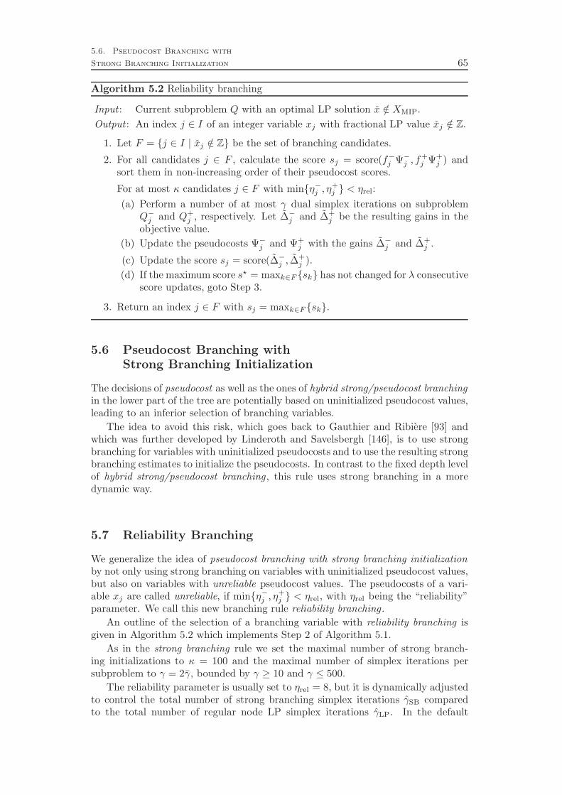
5.6. Pseudocost Branching with
Strong Branching Initialization 65
Algorithm 5.2 Reliability branching
Input : Current subproblem Q with an optimal LP solution x /∈ XMIP.
Output : An index j ∈ I of an integer variable xj with fractional LP value xj /∈ Z.
1. Let F = {j ∈ I | xj /∈ Z} be the set of branching candidates.
2. For all candidates j ∈ F , calculate the score sj = score(f−j Ψ−j , f+j Ψ+
j ) andsort them in non-increasing order of their pseudocost scores.
For at most κ candidates j ∈ F with min{η−j , η+j } < ηrel:
(a) Perform a number of at most γ dual simplex iterations on subproblemQ−j and Q+
j , respectively. Let ∆−j and ∆+j be the resulting gains in the
objective value.
(b) Update the pseudocosts Ψ−j and Ψ+j with the gains ∆−j and ∆+
j .
(c) Update the score sj = score(∆−j , ∆+j ).
(d) If the maximum score s⋆ = maxk∈F{sk} has not changed for λ consecutivescore updates, goto Step 3.
3. Return an index j ∈ F with sj = maxk∈F{sk}.
5.6 Pseudocost Branching withStrong Branching Initialization
The decisions of pseudocost as well as the ones of hybrid strong/pseudocost branchingin the lower part of the tree are potentially based on uninitialized pseudocost values,leading to an inferior selection of branching variables.
The idea to avoid this risk, which goes back to Gauthier and Ribière [93] andwhich was further developed by Linderoth and Savelsbergh [146], is to use strongbranching for variables with uninitialized pseudocosts and to use the resulting strongbranching estimates to initialize the pseudocosts. In contrast to the fixed depth levelof hybrid strong/pseudocost branching , this rule uses strong branching in a moredynamic way.
5.7 Reliability Branching
We generalize the idea of pseudocost branching with strong branching initializationby not only using strong branching on variables with uninitialized pseudocost values,but also on variables with unreliable pseudocost values. The pseudocosts of a vari-able xj are called unreliable, if min{η−j , η
+j } < ηrel, with ηrel being the “reliability”
parameter. We call this new branching rule reliability branching .
An outline of the selection of a branching variable with reliability branching isgiven in Algorithm 5.2 which implements Step 2 of Algorithm 5.1.
As in the strong branching rule we set the maximal number of strong branch-ing initializations to κ = 100 and the maximal number of simplex iterations persubproblem to γ = 2γ, bounded by γ ≥ 10 and γ ≤ 500.
The reliability parameter is usually set to ηrel = 8, but it is dynamically adjustedto control the total number of strong branching simplex iterations γSB comparedto the total number of regular node LP simplex iterations γLP. In the default
66 Branching
parameter settings our goal is to restrict the strong branching simplex iterations toa maximum of γmax
SB = 12 γLP + 100000. If they exceed γSB > γmax
SB , the reliabilityvalue is reduced to ηrel = 0 which turns off strong branching initializations such thatreliability branching becomes equivalent to pseudocost branching . Within the intervalγSB ∈
[12γmax
SB , γmaxSB
]ηrel is linearly decreased from 8 to 1, with the extreme case
ηrel = 1 corresponding to pseudocost branching with strong branching initialization.On the other hand, if γSB is very small, namely γSB < 1
2 γLP, ηrel is increased
proportionally to γLP
γSBsuch that reliability branching resembles strong branching in
the limiting case of ηrel →∞.
5.8 Inference Branching
In a CSP or SAT instance where no objective function is available it does not makesense to base the branching decision on the change in the LP relaxation’s objectivevalue. Therefore one has to use a different measure to estimate the impact of avariable to the given problem instance. One idea is to select a branching variablethat, after tightening its domain, produces the largest number of deductions on othervariables.
Like with LP objective value based branching rules, the impact of a variable interms of deductions can either be calculated directly in a strong branching fashionby explicitly propagating the bound changes of the branching candidates, or bycollecting historical information similar to the pseudocost values. For example, theSAT solver SatZ [143, 144] takes the former approach. The inference branching ruleof SCIP uses the latter idea.
The inference value of a variable xj , j ∈ I, is defined analog to the pseudocostsof Equation (5.4) as
Φ+j =
ϕ+j
ν+j
(5.5)
where ϕ+j is the total number of all inferences deduced after branching upwards
on variable xj , and ν+j is the number of corresponding subproblems Q+
j for which
domain propagation has already been applied. Note that ν+j is very similar to
the pseudocost counter η+j , but it needs not to be the same since there may be
subproblems for which only domain propagation or only LP solving is applied.Additionally, pseudocosts are also collected by strong branching evaluations, whilethe inference history can be populated by probing and other presolving techniques,see Chapter 10.
Like pseudocost branching , the inference branching rule suffers from the fact thatthe most crucial decisions at the top of the search tree are based on very little in-formation, since the inference values are collected during the search. Obviously, onecould overcome this issue by combining explicit inference calculations and historicalinformation analog to the pseudocost branching with strong branching initializationor even the reliability branching rule. However, we do not take this approach inSCIP. For general integer variables we define an uninitialized inference value to bezero. For (the usually more important) binary variables we use the informationof the implication graph and clique table, see Section 3.3.5, to define replacementsfor uninitialized inference values. Let D = (V,A) be the current implication graphas defined in Definition 3.9 and let Q(xj = 1) be the set of cliques the variable iscontained in as positive literal. Now, if an inference value of a binary variable is
5.9. Hybrid Reliability/Inference Branching 67
uninitialized, i.e., ν+j = 0, we define
Φ+j =
∣∣δ−D(xj = 1)
∣∣+ 2 ·
∣∣Q(xj = 1)
∣∣.
Note that the factor 2 applied to the number of cliques is an underestimate of theactual implications represented by the cliques since all cliques in the clique table areat least of cardinality 3.
If probing is used as a presolver, see Section 10.6, the implication graph getspopulated by all implications of binary variables. Therefore, one can see probing inthis regard as a strong branching initialization of the inference values at the rootnode for all binary variables. In this sense, our approach of dealing with uninitial-ized inference values is very similar to pseudocost branching with strong branchinginitialization.
5.9 Hybrid Reliability/Inference Branching
The hybrid reliability/inference branching rule combines the selection criteria of reli-ability branching and inference branching . Additionally, in the presence of conflictanalysis, see Chapter 11, we include the score values of a variable state independentdecaying sum (VSIDS) branching strategy as it is used in SAT solvers, see Moskewiczet al. [168]. This rule prefers variables that have been used in the conflict graphanalysis to produce recent conflict constraints. Finally, we include a score valuewhich is based on the number of infeasible or bound-exceeding subproblems (i.e.,the number of cutoffs) that have been generated due to branching on the respectivevariable.
Let srelij , sinfer
j , sconfj , and scutoff
j be the individual score values for the reliabil-ity branching , inference branching , conflict branching, and cutoff branching rules,respectively. The problem with combining these values into a single score is thatthey operate on completely different scales. In particular, the scale of sreli is highlydependent on the problem instance, namely the objective function. Therefore onehas to apply a normalization step to transform the individual score values onto aunified scale, for which we use the function
g : R≥0 → [0, 1), g(x) =x
x+ 1.
As one can see in Figure 5.1 the function g(·) has its dynamic range roughly in theregion between 0 and 4. It seems reasonable to first scale the different score valuessuch that they are mapped into the dynamic range of g(·) and apply g(·) afterwards.Therefore, we combine the four values with the formula
sj = ωrelig
(
srelij
sreli∅
)
+ ωinferg
(
sinferj
sinfer∅
)
+ ωconfg
(
sconfj
sconf∅
)
+ ωcutoffg
(
scutoffj
scutoff∅
)
in which the s∅ values are the current average values over all variables in the probleminstance. The weights are set to ωreli = 1, ωinfer = ωcutoff = 10−4, and ωconf = 10−2.
Besides the different calculation of the score values, the hybrid reliability/infe-rence branching rule is equal to reliability branching as shown in Algorithm 5.2.Thus, one can view reliability branching as a special case of hybrid reliability/infe-rence branching with ωreli = 1 and ωinfer = ωconf = ωcutoff = 0. Since g(·) is strictlymonotone, the application of g(·) to sreli does not modify the branching variableselection.
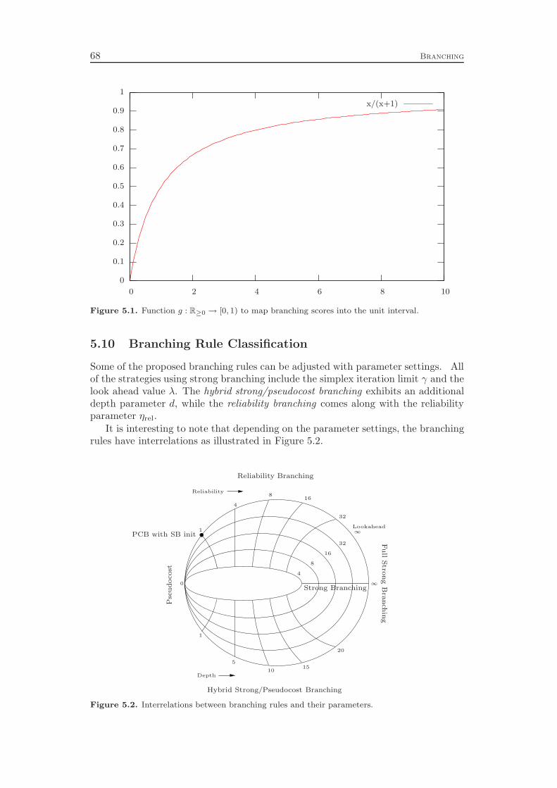
68 Branching
0
0.1
0.2
0.3
0.4
0.5
0.6
0.7
0.8
0.9
1
0 2 4 6 8 10
x/(x+1)
Figure 5.1. Function g : R≥0 → [0, 1) to map branching scores into the unit interval.
5.10 Branching Rule Classification
Some of the proposed branching rules can be adjusted with parameter settings. Allof the strategies using strong branching include the simplex iteration limit γ and thelook ahead value λ. The hybrid strong/pseudocost branching exhibits an additionaldepth parameter d, while the reliability branching comes along with the reliabilityparameter ηrel.
It is interesting to note that depending on the parameter settings, the branchingrules have interrelations as illustrated in Figure 5.2.
Reliability Branching
Pse
ud
oco
st
Hybrid Strong/Pseudocost Branching
Strong Branching
Fu
llS
tron
gB
ran
chin
g
PCB with SB init
Reliability
Depth
Lookahead
0
1
1
4
4
8
8
16
16
32
32
5
1015
20
∞
∞
Figure 5.2. Interrelations between branching rules and their parameters.
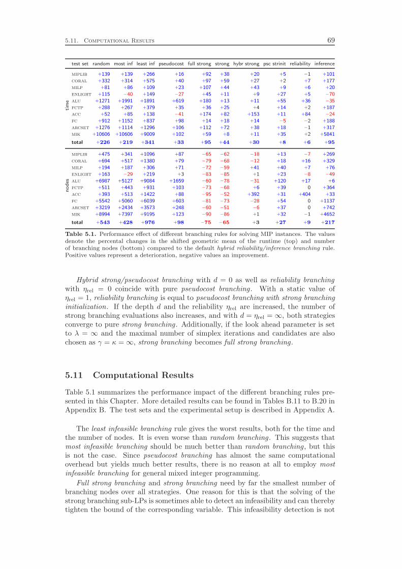
5.11. Computational Results 69
test set random most inf least inf pseudocost full strong strong hybr strong psc strinit reliability inferenceti
me
miplib +139 +139 +266 +16 +92 +38 +20 +5 −1 +101
coral +332 +314 +575 +40 +97 +59 +27 +2 +7 +177
milp +81 +86 +109 +23 +107 +44 +43 +9 +6 +20
enlight +115 −40 +149 −27 +45 +11 +9 +27 +5 −70
alu +1271 +1991 +1891 +619 +180 +13 +11 +55 +36 −35
fctp +288 +267 +379 +35 +36 +25 +4 +14 +2 +187
acc +52 +85 +138 −41 +174 +82 +153 +11 +84 −24
fc +912 +1152 +837 +98 +14 +18 +14 −5 −2 +188
arcset +1276 +1114 +1296 +106 +112 +72 +38 +18 −1 +317
mik +10606 +10606 +9009 +102 +59 +8 +11 +35 +2 +5841
total +226 +219 +341 +33 +95 +44 +30 +8 +6 +95
no
des
miplib +475 +341 +1096 +87 −65 −62 −18 +13 −7 +269
coral +694 +517 +1380 +79 −79 −68 −12 +18 +16 +329
milp +194 +187 +306 +71 −72 −59 +41 +40 +7 +76
enlight +163 −29 +219 +3 −83 −85 +1 +23 −8 −49
alu +6987 +5127 +9084 +1659 −60 −78 −31 +120 +17 +6
fctp +511 +443 +931 +103 −73 −68 +6 +39 0 +364
acc +393 +513 +1422 +88 −95 −52 +392 +31 +404 +33
fc +5542 +5060 +6039 +603 −81 −73 −28 +54 0 +1137
arcset +3219 +2434 +3573 +248 −60 −51 −6 +37 0 +742
mik +8994 +7397 +9195 +123 −90 −86 +1 +32 −1 +4652
total +543 +428 +976 +98 −75 −65 +3 +27 +9 +217
Table 5.1. Performance effect of different branching rules for solving MIP instances. The valuesdenote the percental changes in the shifted geometric mean of the runtime (top) and numberof branching nodes (bottom) compared to the default hybrid reliability/inference branching rule.Positive values represent a deterioration, negative values an improvement.
Hybrid strong/pseudocost branching with d = 0 as well as reliability branchingwith ηrel = 0 coincide with pure pseudocost branching . With a static value ofηrel = 1, reliability branching is equal to pseudocost branching with strong branchinginitialization. If the depth d and the reliability ηrel are increased, the number ofstrong branching evaluations also increases, and with d = ηrel =∞, both strategiesconverge to pure strong branching . Additionally, if the look ahead parameter is setto λ = ∞ and the maximal number of simplex iterations and candidates are alsochosen as γ = κ =∞, strong branching becomes full strong branching .
5.11 Computational Results
Table 5.1 summarizes the performance impact of the different branching rules pre-sented in this Chapter. More detailed results can be found in Tables B.11 to B.20 inAppendix B. The test sets and the experimental setup is described in Appendix A.
The least infeasible branching rule gives the worst results, both for the time andthe number of nodes. It is even worse than random branching . This suggests thatmost infeasible branching should be much better than random branching , but thisis not the case. Since pseudocost branching has almost the same computationaloverhead but yields much better results, there is no reason at all to employ mostinfeasible branching for general mixed integer programming.
Full strong branching and strong branching need by far the smallest number ofbranching nodes over all strategies. One reason for this is that the solving of thestrong branching sub-LPs is sometimes able to detect an infeasibility and can therebytighten the bound of the corresponding variable. This infeasibility detection is not
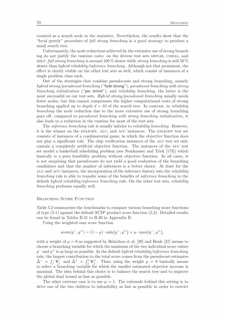
70 Branching
counted as a search node in the statistics. Nevertheless, the results show that the“local greedy” procedure of full strong branching is a good strategy to produce asmall search tree.
Unfortunately, the node reductions achieved by the extensive use of strong branch-ing do not justify the runtime costs: on the diverse test sets miplib, coral, andmilp, full strong branching is around 100 % slower while strong branching is still 50 %slower than hybrid reliability/inference branching . Although not that prominent, theeffect is clearly visible on the other test sets as well, which consist of instances of asingle problem class each.
Out of the strategies that combine pseudocosts and strong branching, namelyhybrid strong/pseudocost branching (“hybr strong”), pseudocost branching with strongbranching initialization (“psc strinit”), and reliability branching , the latter is themost successful on our test sets. Hybrid strong/pseudocost branching usually needsfewer nodes, but this cannot compensate the higher computational costs of strongbranching applied up to depth d = 10 of the search tree. In contrast, in reliabilitybranching the node reduction due to the more extensive use of strong branchingpays off: compared to pseudocost branching with strong branching initialization, italso leads to a reduction in the runtime for most of the test sets.
The inference branching rule is usually inferior to reliability branching . However,it is the winner on the enlight, alu, and acc instances. The enlight test setconsists of instances of a combinatorial game, in which the objective function doesnot play a significant role. The chip verification instances of the alu test set onlycontain a completely artificial objective function. The instances of the acc testset model a basketball scheduling problem (see Nemhauser and Trick [173]) whichbasically is a pure feasibility problem without objective function. In all cases, itis not surprising that pseudocosts do not yield a good evaluation of the branchingcandidates and that the number of inferences is a better choice. At least for thealu and acc instances, the incorporation of the inference history into the reliabilitybranching rule is able to transfer some of the benefits of inference branching to thedefault hybrid reliability/inference branching rule. On the other test sets, reliabilitybranching performs equally well.
Branching Score Function
Table 5.2 summarizes the benchmarks to compare various branching score functionsof type (5.1) against the default SCIP product score function (5.2). Detailed resultscan be found in Tables B.21 to B.30 in Appendix B.
Using the weighted sum score function
score(q−, q+) = (1− µ) ·min{q−, q+}+ µ ·max{q−, q+},
with a weight of µ = 0 as suggested by Bénichou et al. [39] and Beale [37] means tochoose a branching variable for which the minimum of the two individual score valuesq− and q+ is as large as possible. In the default hybrid reliability/inference branchingrule, the largest contribution to the total score comes from the pseudocost estimates∆− = f−j Ψ−j and ∆+ = f+
j Ψ+j . Thus, using the weight µ = 0 basically means
to select a branching variable for which the smaller estimated objective increase ismaximal. The idea behind this choice is to balance the search tree and to improvethe global dual bound as fast as possible.
The other extreme case is to use µ = 1. The rationale behind this setting is todrive one of the two children to infeasibility as fast as possible in order to restrict
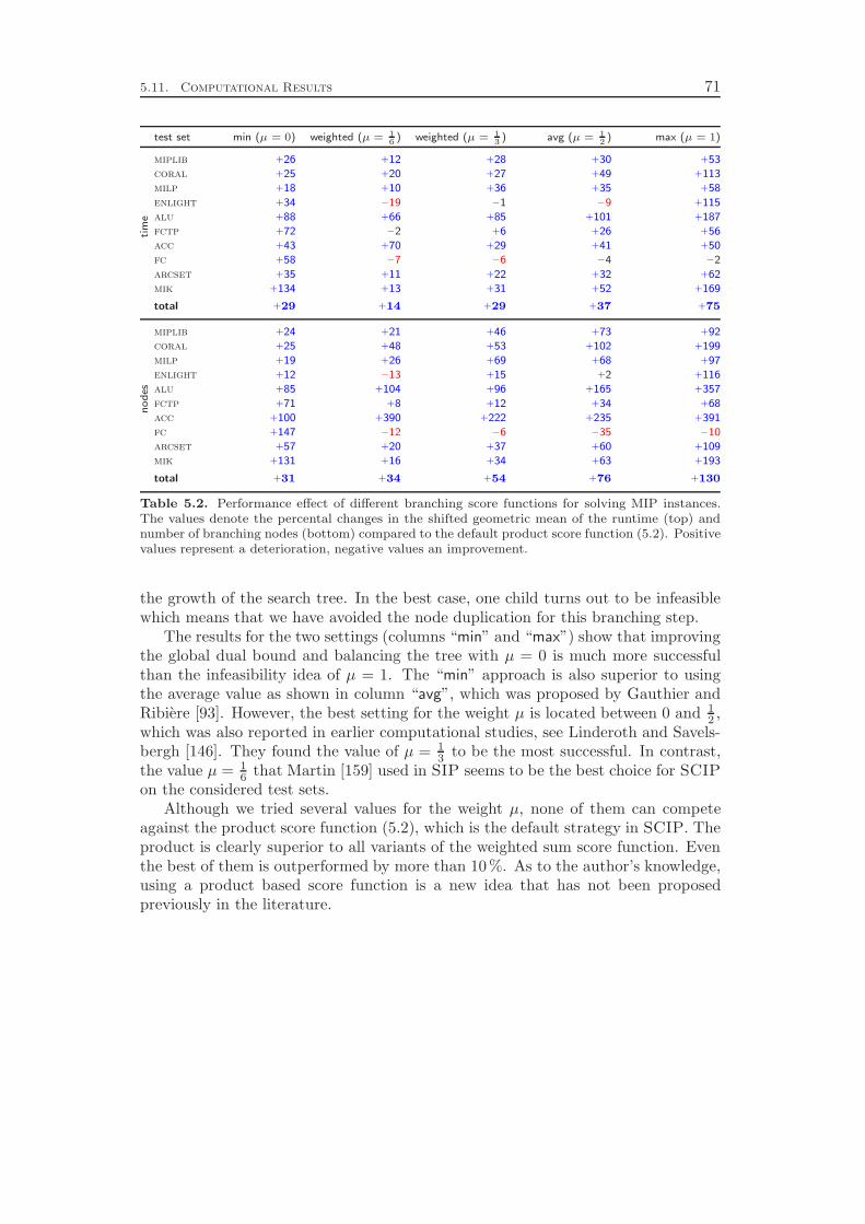
5.11. Computational Results 71
test set min (µ = 0) weighted (µ = 16
) weighted (µ = 13
) avg (µ = 12
) max (µ = 1)ti
me
miplib +26 +12 +28 +30 +53
coral +25 +20 +27 +49 +113
milp +18 +10 +36 +35 +58
enlight +34 −19 −1 −9 +115
alu +88 +66 +85 +101 +187
fctp +72 −2 +6 +26 +56
acc +43 +70 +29 +41 +50
fc +58 −7 −6 −4 −2
arcset +35 +11 +22 +32 +62
mik +134 +13 +31 +52 +169
total +29 +14 +29 +37 +75
no
des
miplib +24 +21 +46 +73 +92
coral +25 +48 +53 +102 +199
milp +19 +26 +69 +68 +97
enlight +12 −13 +15 +2 +116
alu +85 +104 +96 +165 +357
fctp +71 +8 +12 +34 +68
acc +100 +390 +222 +235 +391
fc +147 −12 −6 −35 −10
arcset +57 +20 +37 +60 +109
mik +131 +16 +34 +63 +193
total +31 +34 +54 +76 +130
Table 5.2. Performance effect of different branching score functions for solving MIP instances.The values denote the percental changes in the shifted geometric mean of the runtime (top) andnumber of branching nodes (bottom) compared to the default product score function (5.2). Positivevalues represent a deterioration, negative values an improvement.
the growth of the search tree. In the best case, one child turns out to be infeasiblewhich means that we have avoided the node duplication for this branching step.
The results for the two settings (columns “min” and “max”) show that improvingthe global dual bound and balancing the tree with µ = 0 is much more successfulthan the infeasibility idea of µ = 1. The “min” approach is also superior to usingthe average value as shown in column “avg”, which was proposed by Gauthier andRibière [93]. However, the best setting for the weight µ is located between 0 and 1
2 ,which was also reported in earlier computational studies, see Linderoth and Savels-bergh [146]. They found the value of µ = 1
3to be the most successful. In contrast,
the value µ = 16 that Martin [159] used in SIP seems to be the best choice for SCIP
on the considered test sets.Although we tried several values for the weight µ, none of them can compete
against the product score function (5.2), which is the default strategy in SCIP. Theproduct is clearly superior to all variants of the weighted sum score function. Eventhe best of them is outperformed by more than 10 %. As to the author’s knowledge,using a product based score function is a new idea that has not been proposedpreviously in the literature.

Chapter 6
Node Selection
After a subproblem has been processed, the solving process can continue with anysubproblem that is a leaf of the current search tree. The selection of the subproblemthat should be processed next has two usually opposing goals within the MIP branch-and-bound search:
1. finding good feasible MIP solutions to improve the primal (upper) bound,which helps to prune the search tree by bounding, and
2. improving the global dual (lower) bound.
Besides by employing primal heuristics, feasible MIP solutions can be found as so-lutions to LP relaxations of subproblems that happen to be integral. It can beobserved, see for example Linderoth and Savelsberg [146], that integral LP solutionsare typically found very deep in the search tree. Therefore, to quickly identify feas-ible solutions of a MIP instance, strategies like depth first search seem to be themost natural choice. The second goal, however, is completely disregarded by depthfirst search, since the nodes with the best (i.e., smallest) lower bound are usuallyclose to the root node of the search tree. To improve the global dual bound as fastas possible, one should use best first search which is to always select a leaf with thecurrently smallest dual objective value. Trying to achieve both goals at the sametime leads to a mixture of the two strategies, which is called best first search withplunging.
A variant of best first search is the so-called best estimate search. This strat-egy does not select the node with the best dual bound, but the one with the bestestimated objective value of the feasible solutions contained in the correspondingsubtree. The estimate is calculated from the dual bound and the fractionalities andpseudocost values of the variables (see Section 5.3). The goal of best estimate searchis to find a good, preferably optimal feasible solution as soon as possible. Natu-rally, this strategy can also be combined with depth first search, which leads to bestestimate search with plunging. Finally, one can combine all the three strategies intohybrid versions, for example by applying the selection rules in an interleaving fashionor by using weighted combinations of the individual node selection score values.
In the following sections, we will take a closer look at the different strategies andevaluate them by computational experiments.
6.1 Depth First Search
Depth first search was proposed by Little et al. [149] for the traveling salesmanproblem and by Dakin [71] for mixed integer programming. This node selection rulealways chooses a child of the current node as the next subproblem to be processed.If the current node is pruned and therefore has no children, the search backtracks
to the most recent ancestor that has another unprocessed child left and selects one
73
74 Node Selection
of its children. Thus, one selects always a node from the leaf queue with maximaldepth in the search tree.
Depth first search is the preferred strategy for pure feasibility problems like SATor CSP. Since these problems do not have an objective function, the solving processis solely focused on finding a feasible solution, and there is no need to increase alower objective bound. But besides its ability to identify feasible solutions, depthfirst search has a second advantage: the next subproblem to be processed is almostalways very similar to the current one. Therefore, the subproblem management isreduced to a minimum. In particular, only very small changes have to be applied tothe LP relaxation. If the branching is performed on variables by splitting a bound ofan integer variable into two parts, the only update in the LP is one bound change ofa single variable. This can be done very efficiently in simplex solvers. Most notably,the current basis matrix factorization remains valid for the child problem, therebysaving the time for basis refactorization.
A third advantage of depth first search is its small memory consumption. If thecurrent node is in depth d, then the search tree consists of at most b · d + 1 nodesthat are not yet pruned, where b is the maximal number of children of a node.This means, the number of nodes we have to store for a 2-way branching schemenever exceeds 2dmax +1, with dmax being the maximal depth of the search tree. Forbinary or mixed binary programs, the maximal depth is bounded by dmax ≤ |B| if webranch on variables, which means the memory consumption for node data structuresis linear in the number of binary variables.
Using depth first search as node selection strategy leaves open only one additionalchoice, namely which of the unsolved children of the current node should be processedfirst. SAT solvers like BerkMin [100] try to use this freedom of choice to balancetheir conflict clause databases (see Chapter 11) with respect to the appearance ofthe branching variable and its negation in the conflict clauses. This is basicallyachieved by first selecting the fixing of the branching variable that appears in thelarger number of conflict clauses, since new conflict clauses derived in this subtreecan only contain the negation of the branching variable.
The idea of Martin [159] for mixed integer programming (using the usual branch-ing on integer variables with fractional LP value) is to select the branch that pushesthe LP value of the variable further away from its value in the root node’s LP so-lution. Say, for example, that we branched on variable xj with current LP solutionxj = 2.3, which has an LP solution value of (xR)j = 2.6 in the root node’s relaxation.Martin’s idea is that on the path to the current node the value of the variable hasthe tendency to be pushed towards 2, and that the branch xj ≤ 2 should thereforebe inspected first. Although we did not verify this by thorough computational stud-ies, we experienced that this child selection strategy yields very good results andtherefore adopted it in SCIP.
6.2 Best First Search
Best first search aims at improving the global dual bound as fast as possible byalways selecting a subproblem with the smallest dual bound of all remaining leavesin the tree. As a side-effect, this strategy leads to a minimal number of nodesthat need to be processed, given that the branching rule is fixed. Note that bestfirst search is not uniquely defined as there may be multiple nodes with equal dualbound.
6.3. Best First Search with Plunging 75
Proposition 6.1. Given an instance of a constraint integer program and a fixedbranching strategy in the branch-and-bound Algorithm 2.1, there exists a node se-lection strategy of best first search type which solves the instance in a minimalnumber of nodes.
Proof. Due to the fixed branching strategy, the search tree is uniquely defined, in-cluding all nodes that could be pruned by bounding if the optimal solution value c⋆
was known. A node selection strategy σ defines an order of the nodes in the treesuch that for all nodes Qi with parent p(Qi) we have σ(p(Qi)) < σ(Qi). Let cQi
bethe lower bound of node Qi before it is processed. Certainly, cQi
≥ cp(Qi) with cQbeing the optimal value of a relaxation Qrelax of subproblem Q, for example, the LPrelaxation of Q.
Let σ⋆ be an optimal node selection strategy with respect to the number ofnodes that have to be processed. Assume that σ⋆ is not of best first search type.Then there are node indices i, j with σ(Qi) < σ(Qj) and cQi
> cQj. Since Qi is
processed in the optimal node selection strategy, the optimal value for the CIP mustbe c⋆ ≥ cQi
> cQj. Therefore, Qj cannot be pruned by bounding and must also be
processed. Thus, we can exchange Qi and Qj in the node selection order withoutincreasing the number of processed nodes. By iteratively applying this exchangeprocedure, σ⋆ can be converted into a best first search node selection strategy thatis still optimal.
Note. Although there always exists an optimal best first search node selection strat-egy, not every best first search rule processes a minimal number of nodes. As anexample, assume that L = {Q1,Q2} is the current list of open subproblems, andboth subproblems have a lower bound of cQ1
= cQ2= c < c with c being the value
of the current incumbent solution. Furthermore, suppose that we apply a best firstnode selection strategy that picks Q1 as the next subproblem. If after the processingof Q1 the relaxation value is cQ1
> cQ2, but processing of Q2 leads to cQ2
= cQ2
and the detection of a solution with value c⋆ = cQ2, then we have processed Q1
unnecessarily: if we had processed Q2 first, we would have found the solution andpruned Q1 due to cQ1
≥ c⋆ without processing it.
The best first node selection strategy can be efficiently implemented by storingthe leaves of the search tree in a priority queue, see Section 3.3.6. The questionremains which node one should select if there are multiple nodes that have dualbounds equal to the global dual bound. In order to find good feasible solutionsearly, we select the node with better estimate, see Section 6.4 below. If there arestill ties left, we try to stay close to the previous subproblem and favor child nodesof the current node over its siblings, and siblings over the remaining leaves of thetree.
6.3 Best First Search with Plunging
As said in the introduction of this chapter, best first search leads to a small numberof processed nodes, while depth first search tends to produce feasible solutions earlierand speeds up the node solving process due to the closer resemblance of successivesubproblems. The idea of plunging is to mix both strategies in order to combinetheir benefits. As long as the current node has unprocessed children, one of themis selected as the next node. Otherwise, plunging continues with one of the current
76 Node Selection
node’s siblings. If no more unprocessed children or siblings are available, the currentplunge is completed, and a leaf from the tree with best dual bound is selected.
The branching tree data structures of SCIP are specifically tailored to supportthis strategy, see Section 3.3.6. The children and the siblings of the current nodeare stored separately from the remaining leaves and can therefore easily be accessedand identified. The remaining leaves are stored in a priority queue which enablesefficient access to the best node corresponding to a certain ordering. For best firstsearch the ordering is defined by the dual bounds of the leaves.
Again, the question remains which child or sibling should be processed nextduring plunging. Usually, the child nodes inherit the dual bound of their parentnode, which means that they cannot be differentiated with respect to their dualbounds. As plunging is mainly focused on finding feasible solutions, we apply—asin depth first search—the LP solution guided rule of Martin [159]. We use Martin’srule even if strong branching (see Section 5.4) produced different dual bounds forthe child nodes, which would enable a best first selection.
The largest disadvantage of depth first search is its high risk of processing su-perfluous nodes that would have been pruned if a good solution was known earlier.Plunging has the same property, although to a much smaller extent, since aftereach plunge the search continues with a node of smallest lower bound. Neverthe-less, it might be profitable to prematurely abort a plunge if the local lower boundapproaches the primal bound. This would avoid the processing of some of the su-perfluous nodes, but the disadvantage is that one may miss small improvements inthe primal bound.
The strategy of SCIP is to mainly use plunging for its effect of faster nodeprocessing due to close resemblance of subproblems. The identification of primalsolutions is left to the primal heuristics, namely the diving heuristics which basicallycontinue the plunging outside the branching tree, but apply different variable andvalue selection rules that are particularly tailored for finding feasible solutions; seeChapter 9 for an overview of the primal heuristics included in SCIP. During eachplunge, we perform a certain minimal number of plunging steps, but we abort theplunging after a certain total number of steps or if the local relative gap
γ(Q) =cQ − c
c− c
of the current subproblem Q exceeds the threshold γmax = 0.25. Here, cQ is thelower bound of the subproblem, c is global lower bound, and c is the global upperbound, i.e., the value of the incumbent solution or infinity. The minimal and maximalnumber of plunging steps are adjusted dynamically to be equal to 0.1 · dmax and0.5 · dmax, respectively, with dmax being the maximum depth of all processed nodes.This means that in the beginning of the search almost no plunging is performed, butthe extent of plunging is increased during the course of the algorithm.
6.4 Best Estimate Search
The nodes selected by best first search have good dual bounds, but their LP solutionsare usually far away from integrality. Depth first search quickly leaves the region ofgood objective values but might be able to find feasible solutions faster. Therefore,none of the two node selection rules aims at finding good solutions. This is addressedby best estimate search. This rule calculates estimate values eQ for the feasible
6.5. Best Estimate Search with Plunging 77
solutions that might be contained in the subtrees represented by the leaves Q ofthe tree, and it selects a node that minimizes this estimate. The estimate combinesinformation about the dual bound and the integrality of the LP solution.
The literature basically proposes two different estimate schemes. The bestprojection criterion of Bénichou et al. [39] calculates an estimate
eprojQ = cQ +
(c− cRφ(xR)
)
φ(xQ),
in which cQ is the dual bound of the current subproblem, cR the dual bound of theroot node, c the incumbent solution value, xQ the current LP solution, and xR theLP solution at the root node. The fractionality φ(x) of a vector x ∈ Rn is defined asφ(x) =
∑nj=1 φ(xj) with φ(xj) = min{xj − ⌊xj⌋, ⌈xj⌉ − xj}. The interpretation of
the best projection estimate is that one calculates the objective value increase perunit decrease in the fractionality of the LP solution for the root node and assumesthat the current LP solution can be driven to integrality with the same objectivevalue increase per unit of fractionality. Note that the best projection method needsa globally valid upper bound.
The best estimate rule of Forrest et al. [88] employs the pseudocost values ofthe variables (see Section 5.3) to estimate the increase in the objective value. Thispseudocost-based estimate is defined as
eQ = cQ +∑
j∈I
min{Ψ−j f
−j ,Ψ
+j f
+j
}
with f−j = xj − ⌊xj⌋ and f+j = ⌈xj⌉− xj being the distances to the nearest integers
for the current LP solution value xj for variable xj , and Ψ−j and Ψ+j being the
pseudocost values of variable xj for rounding downwards and upwards, respectively.Assuming that the pseudocosts are reliable indicators for the per unit objectivevalue increase for shifting a variable downwards or upwards, the best estimate rulecalculates the estimated minimum value of a rounded solution.
Linderoth and Savelsbergh [146] give computational indication that the best es-timate rule is superior to the best projection rule. Therefore, we only implementedthe best estimate rule.
6.5 Best Estimate Search with Plunging
As for the best first search node selection, we can combine best estimate search withdepth first search by a plunging strategy. Again, child or sibling nodes are selecteduntil either all of them have been pruned or the plunge is aborted due to the criteriapresented in Section 6.3. As before, the goal is to transfer the node processingspeedup of depth first search regarding the closely resembled successive subproblemsto the more sophisticated best estimate search strategy.
6.6 Interleaved Best Estimate/Best First Search
The aim of best estimate search is to quickly find good feasible solutions. Afteran optimal solution has been found, the node selection strategy has (despite itsinteraction with other solver components) no more impact on the number of nodes
78 Node Selection
that have to be processed, since the remaining nodes of the tree, defined by thebranching strategy, have to be processed anyway and the order does not matter. Dueto time restrictions, however, the user might not want to wait until the optimality ofthe solution has been proven, but is already satisfied with a given quality guarantee.Therefore, the progression of the global dual bound plays a significant role. In thisregard, best estimate search can perform very poor. Suppose the node with the bestdual bound has a large fractionality measure. That would lead to a rather largeestimate for the node, which means that the node is not processed for a very longtime. The global dual bound would stay at the same level as long as this node isnot touched.
The solution to this problem is to interleave best first and best estimate searchand combine this with plunging. The resulting strategy proceeds as best estimatesearch with plunging, but every bestfreq plunge we choose a node with the bestdual bound instead of one with a best estimate as the next subproblem. We usebestfreq = 10 as default value in our implementation.
6.7 Hybrid Best Estimate/Best First Search
A second approach of increasing the importance of the global dual bound in the bestestimate node selection rule is to calculate the node selection score as a weightedsum of the best estimate and best first scores. In this rule we are selecting a node Qthat minimizes
ω eQ + (1− ω)cQ (6.1)
with ω ∈ [0, 1]. Again, this node selection strategy is combined with plunging. Wechose ω = 0.1 as the default, which means that a larger weight is put on the dualbound and the estimate eQ is only influencing the decision among nodes with verysimilar dual bounds.
6.8 Computational Results
In this section we present computational results to compare the various node selec-tion strategies on several sets of mixed integer programming instances. The test setsare described in Appendix A. Detailed results can be found in Tables B.31 to B.40in Appendix B.
Table 6.1 summarizes the benchmark results. As expected, pure best first search(“bfs”) yields the smallest search trees. Note, however, that Proposition 6.1 cannotbe applied since the branching strategy is affected by the order in which the nodesare processed. In particular, the pseudocosts at a certain node will vary for differentnode selection rules. Thus, it is not always the case that best first search needs thefewest branching nodes.
The second expected behavior can also be clearly observed: depth first search(“dfs”) produces much larger search trees than best first search but can compensatethis disadvantage by a faster node processing time. Overall, the performances ofbest first and depth first search are roughly similar.
The column labeled “bfs/plunge” shows that combining best first search and depthfirst search into the best first search with plunging strategy indeed yields the desiredresult: although not as small as for pure best first search, the search trees are much
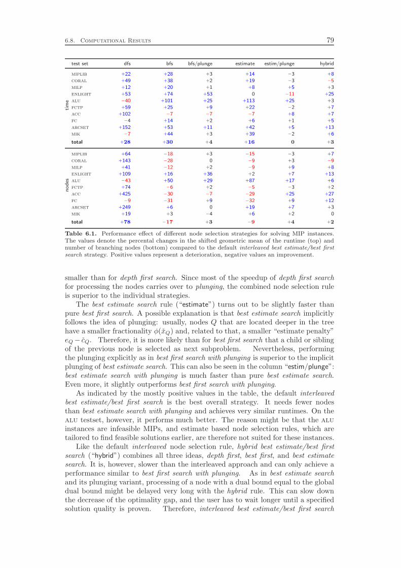
6.8. Computational Results 79
test set dfs bfs bfs/plunge estimate estim/plunge hybridti
me
miplib +22 +28 +3 +14 −3 +8
coral +49 +38 +2 +19 −3 −5
milp +12 +20 +1 +8 +5 +3
enlight +53 +74 +53 0 −11 +25
alu −40 +101 +25 +113 +25 +3
fctp +59 +25 +9 +22 −2 +7
acc +102 −7 −7 −7 +8 +7
fc −4 +14 +2 +6 +1 +5
arcset +152 +53 +11 +42 +5 +13
mik −7 +44 +3 +39 −2 +6
total +28 +30 +4 +16 0 +3
no
des
miplib +64 −18 +3 −15 −3 +7
coral +143 −28 0 −9 +3 −9
milp +41 −12 +2 −9 +9 +8
enlight +109 +16 +36 +2 +7 +13
alu −43 +50 +29 +87 +17 +6
fctp +74 −6 +2 −5 −3 +2
acc +425 −30 −7 −29 +25 +27
fc −9 −31 +9 −32 +9 +12
arcset +249 +6 0 +19 +7 +3
mik +19 +3 −4 +6 +2 0
total +78 −17 +3 −9 +4 +2
Table 6.1. Performance effect of different node selection strategies for solving MIP instances.The values denote the percental changes in the shifted geometric mean of the runtime (top) andnumber of branching nodes (bottom) compared to the default interleaved best estimate/best firstsearch strategy. Positive values represent a deterioration, negative values an improvement.
smaller than for depth first search. Since most of the speedup of depth first searchfor processing the nodes carries over to plunging, the combined node selection ruleis superior to the individual strategies.
The best estimate search rule (“estimate”) turns out to be slightly faster thanpure best first search. A possible explanation is that best estimate search implicitlyfollows the idea of plunging: usually, nodes Q that are located deeper in the treehave a smaller fractionality φ(xQ) and, related to that, a smaller “estimate penalty”eQ− cQ. Therefore, it is more likely than for best first search that a child or siblingof the previous node is selected as next subproblem. Nevertheless, performingthe plunging explicitly as in best first search with plunging is superior to the implicitplunging of best estimate search. This can also be seen in the column “estim/plunge”:best estimate search with plunging is much faster than pure best estimate search.Even more, it slightly outperforms best first search with plunging.
As indicated by the mostly positive values in the table, the default interleavedbest estimate/best first search is the best overall strategy. It needs fewer nodesthan best estimate search with plunging and achieves very similar runtimes. On thealu testset, however, it performs much better. The reason might be that the aluinstances are infeasible MIPs, and estimate based node selection rules, which aretailored to find feasible solutions earlier, are therefore not suited for these instances.
Like the default interleaved node selection rule, hybrid best estimate/best firstsearch (“hybrid”) combines all three ideas, depth first, best first, and best estimatesearch. It is, however, slower than the interleaved approach and can only achieve aperformance similar to best first search with plunging. As in best estimate searchand its plunging variant, processing of a node with a dual bound equal to the globaldual bound might be delayed very long with the hybrid rule. This can slow downthe decrease of the optimality gap, and the user has to wait longer until a specifiedsolution quality is proven. Therefore, interleaved best estimate/best first search

80 Node Selection
seems to be the better choice even though it might be possible to improve theperformance of hybrid best estimate/best first search by altering the weight ω ∈ [0, 1]in Equation (6.1).
Note. In the version of SCIP used in this thesis, there is a significant performancebottleneck associated with long leaf queues and node selection rules that are notbased on best first search. Thus, the performance of best estimate, best estimatewith plunging, hybrid best estimate/best first search, and the default interleaved bestestimate/best first search suffers from that issue on instances that take many nodesand produce large leaf queues during the run. In particular, many of the instancesin enlight, alu, and mik are of this type. Therefore, the “true” performance ofthe estimate based node selection rules on these test sets would be better than thevalues in Table 6.1 indicate.
Child Selection
As the default node selection strategy involves plunging, we have to define a childselection rule in order to decide which of the two children of the current node shouldbe processed next. The main goal of the child selection is to pick a direction whichleads to the finding of a feasible solution, preferably of small objective value. Wecompare the following strategies:
⊲ Downwards selection always chooses the downwards branch xj ≤ ⌊xj⌋.
⊲ Upwards selection always chooses the upwards branch xj ≥ ⌈xj⌉.
⊲ Pseudocost selection prefers the direction that yields a smaller pseudocost esti-mate f−j Ψ−j or f+
j Ψ+j for the LP objective value deterioration, see Section 5.3.
The idea is to guide the search into the area of better objective values.
⊲ LP value selection means to round the branching variable xj to the integer thatis closer to its current LP solution value xj . Thus, it selects the downwardsbranch if f−j = xj − ⌊xj⌋ ≤
12
and the upwards branch otherwise.
⊲ Root LP value selection denotes the idea of Martin [159] which we alreadymentioned in Section 6.1. It compares the current LP value xj of the branchingvariable to its LP value (xR)j in the root node and supports the movementof the value in its current direction: if xj ≤ (xR)j , the variable is brancheddownwards. Otherwise, the upwards branch is inspected first.
⊲ Inference selection chooses the direction in which the branching variable hasa larger inference history value Φ−j or Φ+
j . These values denote the averagenumber of deductions derived from branching the variable into the respectivedirection (see Section 5.8). The hope is that the branch with larger infer-ence history value produces more domain propagations and thus a smallersubproblem for which it is easier to either find a feasible solution or prove theinfeasibility.
⊲ Hybrid inference/root LP value selection is a combination of the inference androot LP value selection rules. It chooses the downwards branch if
(Φ−j + ǫ) · ((xR)j − xj + 1) ≥ (Φ+j + ǫ) · (xj − (xR)j + 1) (6.2)

6.8. Computational Results 81
test set down up pseudocost LP value root LP value inferenceti
me
miplib +23 0 +12 +7 0 +4
coral +10 −11 +6 −2 −5 −4
milp +14 −5 +10 +12 −8 −5
enlight −1 +3 −2 −11 −8 +3
alu −12 −3 +11 +5 +41 −12
fctp +4 −7 +4 +6 −6 −2
acc −19 −1 +20 −15 +13 −7
fc +1 −3 −5 −3 −4 −1
arcset −2 +3 +6 +1 +6 +4
mik −8 +8 +19 +17 +2 −1
total +11 −5 +9 +4 −3 −2
no
des
miplib +18 −1 −8 +1 −2 −4
coral +14 −19 −1 −9 −14 +1
milp +8 −9 +10 +15 −9 −12
enlight −4 +20 −3 −9 −3 +7
alu −6 −20 +27 +3 +29 +6
fctp +2 −11 −2 −1 −9 −2
acc −13 +35 +64 −18 +21 +27
fc +4 −1 −9 +1 −7 +3
arcset +5 −2 +5 0 +7 +3
mik +13 −5 +12 +20 +12 −5
total +10 −9 +2 +1 −6 −3
Table 6.2. Performance effect of different child selection strategies for solving MIP instances. Thevalues denote the percental changes in the shifted geometric mean of the runtime (top) and numberof branching nodes (bottom) compared to the default hybrid inference/root LP value selection.Positive values represent a deterioration, negative values an improvement.
and the upwards branch otherwise. Here, Φ−j ,Φ+j ∈ R≥0 are the inference
history values for the downwards and upwards direction, respectively, andǫ = 10−9 is the zero tolerance. The selection Inequality (6.2) means that avariable that has moved at least by one unit downwards or upwards from theroot node to the current subproblem will be pushed further into that direction,independent from the inference values. On the other hand, the inference valuesdominate the selection for variables with current LP values xj that are closeto their root LP values (xR)j .
Table 6.2 depicts a summary of the experiments. Appendix B provides detailedresults in Tables B.41 to B.50. The comparison of the pure downwards (“down”)and upwards (“up”) preferences shows that consequentially branching upwards isclearly superior, both in the solving time and the number of branching nodes. Apossible explanation is that most MIP instances contain binary variables that rep-resent decisions for which the “yes” case (i.e., setting xj = 1) has a much largerimpact on the model as the “no” case (i.e., xj = 0). It seems natural that taking thecrucial decisions early by fixing a variable to xj = 1 gives better chances to end upwith a feasible solution. In contrast, postponing the crucial decisions by first rulingout some options with xj = 0 most probably leads to a situation in which we cannotsatisfy all constraints with the remaining alternatives.
The bad performance of the pseudocost selection rule (“pseudocost”) is somewhatsurprising as it seems to be the natural choice in the spirit of best first and bestestimate search. On the other hand, many MIP models have costs associated tosetting a binary variable to xj = 1. Thus, upwards pseudocosts tend to be largerthan downwards pseudocosts, such that the pseudocost selection rule is more similarto downwards selection than to upwards selection. Therefore, the above explanationfor the inferior performance of downwards selection also applies to the pseudocost
82 Node Selection
based rule.The LP value selection, although better than pseudocost and downwards selec-
tion, is also inferior to the upwards selection rule. In contrast, the root LP valueselection strategy of Martin [159] is comparable to upwards selection but has theadvantage that it is insensitive against complementation: if we complement all inte-ger variables of a model by setting x′j := lj + uj − xj for j ∈ I (assuming that thebounds are finite), the upwards selection rule would turn into the inferior downwardsselection while the root LP value selection strategy would produce the same resultsas before—at least if all other components of the solver would behave equivalentlyin the complemented variable space.
The inference selection rule is another alternative to upwards selection of similarperformance. As the root LP value selection, it is invariant under variable com-plementation. However, it is more tailored to pure feasibility problems withoutmeaningful objective function since the inference values are based on feasibility ar-guments. In contrast, the LP solution values include both feasibility and optimalityconsiderations. The effect can be seen on the alu and acc instances. The alutest set consists of infeasible MIPs with an artificial objective function, while acc isa collection of basically pure feasibility problems without objective function. Here,inference selection performs much better than root LP value selection. For the othertest sets, however, inference selection is slightly inferior to root LP value selection.
The default strategy, hybrid inference/root LP value selection, also achieves simi-lar performance as upwards selection, root LP value selection, and inference selection.As one can see from the negative values in the columns of the other three rules, how-ever, it is slightly inferior. The attempt to combine the positive effects of root LPvalue selection and inference selection did not succeed. It might be that a differentway to combine the two ideas results in an improved performance. In particular, itseems that Inequality (6.2) is biased too much towards the inference history valuesΦ−j and Φ+
j . Therefore, one should increase the summand ǫ in the inequality to amuch larger value in order to put more weight on the root LP value difference.
Chapter 7
Domain Propagation
Domain propagation denotes the task of tightening the domains of variables byinspecting the constraints and the current domains of other variables at a localsubproblem in the search tree. In the MIP community, this process is usually callednode preprocessing. In fact, one can see domain propagation as a restricted versionof presolving, see Chapter 10. The main restriction for the operations applied tolocal nodes is that they must not modify the constraints. In particular, the deletionof variables is not allowed. Instead, one only tightens the domains of the variables,since this can be done without a large bookkeeping and LP management overhead.
Since the LP relaxation is not able to handle holes inside a domain, MIP solversare only using bound propagation, i.e., one tries to deduce tighter lower and upperbounds for the variables.
Besides the integrality restrictions, there is only one type of constraints in amixed integer program, namely the linear constraints. Therefore, the domainpropagation methods implemented in the linear constraint handler are a supersetof the methods for the more specialized constraint classes like the knapsack or theset covering constraints. The structure of these specific constraints can, however, beexploited in order to implement more efficient domain propagation algorithms.
In addition to the constraint based (primal) domain propagation techniques,SCIP features two dual domain reduction methods that are driven by the objectivefunction, namely the objective propagation and the root reduced cost strengthening.
7.1 Linear Constraints
In SCIP we treat linear constraints in the form
β ≤ aTx ≤ β
with the left and right hand sides β, β ∈ R∪{±∞} and a ∈ Rn being the coefficientsof the constraint. Obviously, equations can be modeled by β = β. For inequalitiesone has typically either β = −∞ or β = +∞, but so-called ranged rows with bothsides being finite and β < β are also possible.
Bound propagation for linear constraints in SCIP is performed as explained inthe “basic preprocessing techniques” of Savelsbergh [199]. The main idea is very sim-ple, but the implementation gets a little more involved if infinite bounds, numericalissues, and runtime performance have to be considered.
The most important notion in this regard is the concept of activity bounds:
Definition 7.1 (activity bounds). Given a linear constraint β ≤ aTx ≤ β, let
α := min{aTx | l ≤ x ≤ u} and α := max{aTx | l ≤ x ≤ u}
be the minimal and maximal activity aTx of the linear constraint with respect tothe local bounds l ≤ x ≤ u of the current subproblem Q. The values α and α are
83
84 Domain Propagation
called activity bounds. Furthermore, let
αj := min{aTx− ajxj | l ≤ x ≤ u} and αj := max{aTx− ajxj | l ≤ x ≤ u}
be the activity bound residuals for the scalar product aTx over all variables but xj .
The activity bounds and the residuals can be easily calculated by inserting thelower or upper bounds of the variables into the product aTx, depending on the signof the coefficients aj . Note that they can be infinite if the local bounds l, u of thevariables are infinite.
The propagations are based on the following observations:
1. If β ≤ α, the left hand side is redundant and can be replaced by −∞ withoutchanging the set of feasible solutions in the subproblem or worsening the dualbound of the LP relaxation.
2. If α ≤ β, the right hand side is redundant and can be replaced by +∞.
3. If β ≤ α and α ≤ β, the constraint is redundant and can be removed.
4. If β > α or α > β, the constraint cannot be satisfied within the local boundsand the current subproblem is infeasible.
5. For all j = 1, . . . , n we have
β − αj
aj
≤ xj ≤β − αj
aj
if aj > 0 and
β − αj
aj
≤ xj ≤β − αj
aj
if aj < 0,
and we can tighten the bounds of xj accordingly. If xj is an integer variable,j ∈ I, the lower bounds can be rounded up and the upper bounds can berounded down.
Inside domain propagation, we only apply Reductions 3 to 5. Despite removingsome degeneracies in the LP there is no benefit in relaxing the constraint sides,but the additional management overhead would be considerable. The redundancydetection of Reduction 3, however, is useful since we can completely ignore suchconstraints in future propagations within the whole subtree defined by the currentsubproblem.
It is easy to see that the repeated application of Reductions 4 and 5 suffices toobtain bound consistency, see Definition 2.7 on page 22. Although it is very likelythat the following propositions are old results, we did not find them in the literature.Therefore, we provide proofs.
Proposition 7.2. A linear constraint β ≤ aTx ≤ β on variables x ∈ Rn, xj ∈ Z for
j ∈ I, with bounds l ≤ x ≤ u, lj , uj ∈ R, lj , uj ∈ Z for j ∈ I, is bound consistent ifand only if Reductions 4 and 5 cannot be applied to detect infeasibility or to tightena variable’s domain.
Proof. Since all domains of the variables are non-empty, bound consistency impliesthat there is a vector x ∈ [l, u] with β ≤ aT x ≤ β. Therefore, β ≤ aT x ≤ α andα ≤ aT x ≤ β, which means that Reduction 4 cannot be applied. Assume that bound

7.1. Linear Constraints 85
consistency holds, but Reduction 5 can be applied on variable xj . Consider the case
aj > 0 and (β − αj)/aj > lj . Bound consistency yields a feasible solution x with
xj = lj . Then we have
aj lj < β − αj ≤ β − (aT x− aj xj) = β − aT x+ aj lj ≤ aj lj ,
which is a contradiction. The other three cases can be shown analogously.Now suppose that neither Reduction 4 nor Reduction 5 can be applied. In order
to prove bound consistency, we have to show that for each bound lj , uj , j ∈ N , there
exists a (potentially fractional) support vector x ∈ [l, u] with xj = lj or xj = uj ,respectively, that satisfies the constraint. Consider variable xj with aj > 0 and its
lower bound lj . Let
xmink :=
lj if k = j
lk if ak ≥ 0
uk if ak < 0
and xmaxk :=
lj if k = j
uk if ak ≥ 0
lk if ak < 0
.
Since Reduction 4 is not applicable, we have
aTxmin = aj lj + αj = α ≤ β,
and because Reduction 5 is not applicable, it follows
aTxmax = aj lj + αj ≥ β.
If one of xmin or xmax is contained in [β, β], it is a valid support vector for lj , andwe are done. Otherwise, the only remaining possibility is
aTxmin < β ≤ β < aTxmax.
In this case, consider the affine linear function
α(t) = aT (xmin + t(xmax − xmin)).
This is a continuous function α : [0, 1] → R with α(0) < β ≤ β < α(1). Therefore,there exists t⋆ ∈ (0, 1) with β ≤ α(t⋆) ≤ β, and the vector
x⋆ = xmin + t⋆(xmax − xmin)
is a valid support vector for lj . The other cases for upper bounds uj and negativecoefficients aj follow with analogous reasoning.
In the case that one of the constraint sides β or β is infinite, we can even achievethe stronger notion of interval consistency by applying Reductions 4 and 5:
Corollary 7.3. A linear constraint β ≤ aTx or aTx ≤ β on variables x ∈ Rn,xj ∈ Z for j ∈ I, with bounds l ≤ x ≤ u, lj , uj ∈ R, lj , uj ∈ Z for j ∈ I, is intervalconsistent if and only if Reductions 4 and 5 cannot be applied to detect infeasibilityor to tighten a variable’s domain.
Proof. In the proof of Proposition 7.2 the case
aTxmin < β ≤ β < aTxmax
cannot appear. If β = −∞, the vector xmin is integral for j ∈ I and supports lj . If
β = +∞, the vector xmax is integral for j ∈ I and supports lj .

86 Domain Propagation
Unfortunately, there is little hope for an efficient algorithm to achieve intervalconsistency in the general case of linear constraints:
Proposition 7.4. Deciding interval consistency for linear constraints of the formβ ≤ aTx ≤ β on variables xj ∈ [lj , uj ] and xj ∈ Z for j ∈ I is NP-complete.
Proof. We provide a reduction from the subset sum problem which is NP-complete(see Garey and Johnson [92]). Given a set of integers aj ∈ Z>0, j = 1, . . . , n, andan integer b ∈ Z, the task of the subset sum problem is to decide whether there is asubset S ⊆ N = {1, . . . , n} with
∑
j∈S aj = b. For b = 0 or b = aT1, the instance
has the trivial solutions S = ∅ or S = N , respectively, and for b < 0 or b > aT1, the
instance is obviously infeasible. Thus, we assume 0 < b < aT1.
Given such an instance (a, b) of the subset sum problem, consider the linearconstraint
0 ≤ −by − (aT1)z + aTx ≤ 0 (7.1)
with domains y, z, xj ∈ {0, 1}, j ∈ N . The vectors (y = 0, z = 0, x = 0) and (y =0, z = 1, x = 1) are feasible integral solutions that support the lower bounds ly =lz = lxj
= 0, j ∈ N , and the upper bounds uz = uxj= 1, j ∈ N , respectively. Thus,
Constraint (7.1) is interval consistent if and only if there exists a feasible integralsolution (y⋆, z⋆, x⋆) with y⋆ = 1. Such a solution must have z⋆ = 0, because b > 0.Therefore, interval consistency of Constraint (7.1) is equivalent to the existence ofx⋆ ∈ {0, 1}n with aTx⋆ = b, which in turn is equivalent to the existence of S ⊆ Nwith
∑
j∈S aj = b.
Propositions 7.2 and 7.4 provide the basic theoretical background for domainpropagation of linear constraints. In the remaining part of the section, we will focuson the implementational issues.
With respect to performance, the most crucial parts are to update the activitybounds α and α instead of recalculating them from scratch at every node and toonly process those constraints where the activity bounds have been changed sincethe last propagation round. In order to accomplish these goals, the linear constrainthandler interacts with an event handler (see Section 3.1.10) to update α and α andto mark each constraint that is affected by a bound change of a variable.
The contributions of infinite bounds lj and uj to α and α are accumulated inseparate counters. These counters are updated whenever a bound of a variableswitches between a finite and an infinite value. If the counter is positive, the actualvalue stored in α or α is ignored and instead treated as infinity.
Tightened bounds deduced by one constraint are used in the domain propagationof other constraints to deduce further bound tightenings. Due to this iterative na-ture, numerical rounding errors can easily accumulate and produce wrong results, inparticular if coefficients of very different magnitude are involved in the calculations.To avoid numerical errors, we slightly relax the newly calculated bounds lj and uj
by usinglj ← 10−5⌊105lj + δ⌋ and uj ← 10−5⌈105uj − δ⌉ (7.2)
with δ = 10−6 being the feasibility tolerance parameter. This operation rounds(within the feasibility tolerance) the values to the five most significant digits afterthe decimal point.
A risk of wasting time on iterated domain propagation originates from generalinteger variables with large domains. Consider the artificial example
0.2 ≤ x− y ≤ 0.8
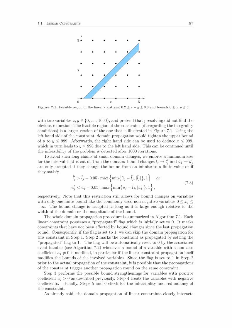
7.1. Linear Constraints 87
x
y
0
5
5
Figure 7.1. Feasible region of the linear constraint 0.2 ≤ x− y ≤ 0.8 and bounds 0 ≤ x, y ≤ 5.
with two variables x, y ∈ {0, . . . , 1000}, and pretend that presolving did not find theobvious reduction. The feasible region of the constraint (disregarding the integralityconditions) is a larger version of the one that is illustrated in Figure 7.1. Using theleft hand side of the constraint, domain propagation would tighten the upper boundof y to y ≤ 999. Afterwards, the right hand side can be used to deduce x ≤ 999,which in turn leads to y ≤ 998 due to the left hand side. This can be continued untilthe infeasibility of the problem is detected after 1000 iterations.
To avoid such long chains of small domain changes, we enforce a minimum sizefor the interval that is cut off from the domain: bound changes lj → l′j and uj → u′jare only accepted if they change the bound from an infinite to a finite value or ifthey satisfy
l′j > lj + 0.05 ·max{
min{uj − lj , |lj |
}, 1}
or
u′j < uj − 0.05 ·max{
min{uj − lj , |uj |
}, 1}
,(7.3)
respectively. Note that this restriction still allows for bound changes on variableswith only one finite bound like the commonly used non-negative variables 0 ≤ xj ≤+∞. The bound change is accepted as long as it is large enough relative to thewidth of the domain or the magnitude of the bound.
The whole domain propagation procedure is summarized in Algorithm 7.1. Eachlinear constraint possesses a “propagated” flag which is initially set to 0. It marksconstraints that have not been affected by bound changes since the last propagationround. Consequently, if the flag is set to 1, we can skip the domain propagation forthis constraint in Step 1. Step 2 marks the constraint as propagated by setting the“propagated” flag to 1. The flag will be automatically reset to 0 by the associatedevent handler (see Algorithm 7.2) whenever a bound of a variable with a non-zerocoefficient aj 6= 0 is modified, in particular if the linear constraint propagation itselfmodifies the bounds of the involved variables. Since the flag is set to 1 in Step 2prior to the actual propagation of the constraint, it is possible that the propagationsof the constraint trigger another propagation round on the same constraint.
Step 3 performs the possible bound strengthenings for variables with positivecoefficient aj > 0 as described previously. Step 4 treats the variables with negativecoefficients. Finally, Steps 5 and 6 check for the infeasibility and redundancy ofthe constraint.
As already said, the domain propagation of linear constraints closely interacts

88 Domain Propagation
Algorithm 7.1 Domain Propagation for Linear Constraints
Input : Linear constraint β ≤ aTx ≤ β, current local bounds l ≤ x ≤ u, andcurrent activity bounds α and α.
Output : Tightened local bounds for x.
1. If the constraint is already marked as propagated, abort.
2. Mark the constraint as propagated.
3. For all variables xj with aj > 0:
(a) Calculate residual activities αj := α− aj lj and αj := α− ajuj .
(b) If αj > −∞ and β < +∞:i. Set u′j := (β − αj)/aj .
ii. Set u′j := 10−5⌈105u′j − δ⌉.
iii. If j ∈ I, set u′j := ⌊u′j + δ⌋.
iv. If u′j < uj − 0.05 ·max{
min{uj − lj , |uj |
}, 1}
, tighten uj := u′j .
(c) If αj < +∞ and β > −∞:i. Set l′j := (β − αj)/aj .
ii. Set l′j := 10−5⌊105l′j + δ⌋.
iii. If j ∈ I, set l′j := ⌈l′j − δ⌉.
iv. If l′j > lj + 0.05 ·max{
min{uj − lj , |lj |
}, 1}
, tighten lj := l′j .
4. For all variables xj with aj < 0:
(a) Calculate residual activities αj := α− aj uj and αj := α− aj lj .
(b) If αj > −∞ and β < +∞:i. Set l′j := (β − αj)/aj .
ii. Set l′j := 10−5⌊105l′j + δ⌋.
iii. If j ∈ I, set l′j := ⌈l′j − δ⌉.
iv. If l′j > lj + 0.05 ·max{
min{uj − lj , |lj |
}, 1}
, tighten lj := l′j .
(c) If αj < +∞ and β > −∞:i. Set u′j := (β − αj)/aj .
ii. Set u′j := 10−5⌈105u′j − δ⌉.
iii. If j ∈ I, set u′j := ⌊u′j + δ⌋.
iv. If u′j < uj − 0.05 ·max{
min{uj − lj , |uj |
}, 1}
, tighten uj := u′j .
5. If β > α or α > β, the current subproblem is infeasible.
6. If β ≤ α and α ≤ β, delete the constraint from the current subproblem.
with an event handler, which is shown in Algorithm 7.2. This event handler catchesall bound changes that are applied on variables that appear with non-zero coefficientaj 6= 0 in the constraint. Whenever such a bound change was performed, the eventhandler updates the activity bounds and marks the constraint such that it will bepropagated again in the next propagation round.
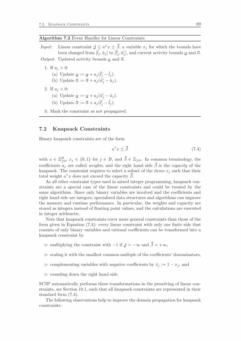
7.2. Knapsack Constraints 89
Algorithm 7.2 Event Handler for Linear Constraints
Input : Linear constraint β ≤ aTx ≤ β, a variable xj for which the bounds have
been changed from [lj , uj ] to [l′j , u′j ], and current activity bounds α and α.
Output : Updated activity bounds α and α.
1. If aj > 0:
(a) Update α := α+ aj(l′j − lj).
(b) Update α := α+ aj(u′j − uj).
2. If aj < 0:
(a) Update α := α+ aj(u′j − uj).
(b) Update α := α+ aj(l′j − lj).
3. Mark the constraint as not propagated.
7.2 Knapsack Constraints
Binary knapsack constraints are of the form
aTx ≤ β (7.4)
with a ∈ ZB≥0, xj ∈ {0, 1} for j ∈ B, and β ∈ Z≥0. In common terminology, the
coefficients aj are called weights, and the right hand side β is the capacity of theknapsack. The constraint requires to select a subset of the items xj such that theirtotal weight aTx does not exceed the capacity β.
As all other constraint types used in mixed integer programming, knapsack con-straints are a special case of the linear constraints and could be treated by thesame algorithms. Since only binary variables are involved and the coefficients andright hand side are integers, specialized data structures and algorithms can improvethe memory and runtime performance. In particular, the weights and capacity arestored as integers instead of floating point values, and the calculations are executedin integer arithmetic.
Note that knapsack constraints cover more general constraints than those of theform given in Equation (7.4): every linear constraint with only one finite side thatconsists of only binary variables and rational coefficients can be transformed into aknapsack constraint by
⊲ multiplying the constraint with −1 if β > −∞ and β = +∞,
⊲ scaling it with the smallest common multiple of the coefficients’ denominators,
⊲ complementing variables with negative coefficients by xj := 1− xj , and
⊲ rounding down the right hand side.
SCIP automatically performs these transformations in the presolving of linear con-straints, see Section 10.1, such that all knapsack constraints are represented in theirstandard form (7.4).
The following observations help to improve the domain propagation for knapsackconstraints:

90 Domain Propagation
Algorithm 7.3 Domain Propagation for Knapsack Constraints
Input : Knapsack constraint aTx ≤ β, current local bounds l ≤ x ≤ u, and currentminimal activity α.
Output : Tightened local bounds for x.
1. If the constraint is already marked as propagated, abort.
2. Mark the constraint as propagated.
3. If α > β, the current subproblem is infeasible.
4. Make sure that the coefficients are sorted such that aj1 ≥ aj2 ≥ . . ..
5. Set w0 := 0.
6. For k = 1, . . . , |B|:
(a) If ajk≤ β − α, break the loop.
(b) If ljk= 0, set ujk
:= 0 and w0 := w0 + ajk.
7. If∑
j∈B aj − w0 ≤ β, delete the constraint from the current subproblem.
1. The only propagation that can be applied is
lj = 0 ∧ α+ aj > β → uj = 0.
2. If we cannot fix a variable xj with lj = 0 to zero, it is not possible to applypropagations on variables xk with ak ≤ aj .
Due to Observation 1, we do not need to track the maximal activity α for knap-sack constraints. The maximal activity can be used to detect redundancy of theconstraint, but this does not justify the additional overhead for tracking its value.Observation 2 indicates that we should sort the variables by non-increasing weightaj and stop the propagation process if we reach an index j where α + aj ≤ β.Note that the propagation only fixes variables to zero and thus the minimal activityα does not change during the propagation. Therefore, the propagation can be im-plemented as a simple scan through the weights which fixes all variables to zero forwhich lj = 0 and aj > β − α. It is shown in Algorithm 7.3.
Steps 1 and 2 check and set the “propagate” flag as in the linear constraintpropagation. Step 3 checks for infeasibility due to the exceedance of the capacityby the variables currently fixed to one. Step 4 sorts the variables by non-increasingweight. Usually, this has only to be performed once during the whole solving process.It might, however, happen in presolving that some coefficients are modified, seeSection 10.2. Since domain propagation is called as a subroutine of the presolvingalgorithm, the sorting may therefore be performed multiple times.
The local variable w0 sums up the weights of variables that are fixed to zero. Itis initialized in Step 5 and updated during the propagation loop in Step 6. Note,however, that it is not calculated exactly if the loop is aborted prematurely. There-fore, the redundancy detection in Step 7 can miss certain cases. The advantage ofthis approach is that we usually can abort the propagation loop at the first iterationand the work spent in the domain propagation algorithm is very low.
As the linear constraint handler, the knapsack constraint handler interacts withan event handler that tracks the bound changes of the involved variables, see Algo-rithm 7.4. In contrast to the event handler for linear constraints, it only needs
7.3. Set Partitioning and Set Packing Constraints 91
Algorithm 7.4 Event Handler for Knapsack Constraints
Input : Knapsack constraint aTx ≤ β, a variable xj for which the lower bound has
been changed from lj to l′j , and current minimal activity α.
Output : Updated minimal activity α.
1. Update α := α+ aj(l′j − lj).
2. Mark the constraint as not propagated.
to catch changes on the lower bounds, because all weights are non-negative andthe maximal activity does not need to be updated. The event handler updates theminimal activity as usual and marks the constraint as not being propagated.
7.3 Set Partitioning and Set Packing Constraints
Set partitioning and set packing constraints are used to model restrictions in whichfrom a certain set of items exactly one or at most one, respectively, has to beselected. Such constraints are very common in several applications, for example tomodel the graph coloring problem (see Mehrotra and Trick [163], or Hansen, Labbé,and Schindl [113]). They can be stated as
∑
j∈S
xj = 1 (set partitioning)
and ∑
j∈S
xj ≤ 1 (set packing),
with binary variables xj ∈ {0, 1}, j ∈ S, and S ⊆ B. As for knapsack constraints,scaling of the equation or inequality and complementing some of the binary variablesmay help to convert a general linear constraint into the form of a set partitioning orset packing constraint.
As they are specializations of linear constraints, set partitioning and set packingconstraints could be dealt with by the linear constraint handler. However, since allcoefficients of included variables are 1 and the left and right hand sides are also fixed,the constraint data only consists of the set of included variables and can therefore bestored much more compactly than in the linear constraint handler. More important,domain propagation can be implemented more efficiently.
In the set packing case, there is only one possibility of domain propagation,namely
xk = 1 → ∀j ∈ S \ {k} : xj = 0.
For set partitioning, the additional propagation rule
∀j ∈ S \ {k} : xj = 0 → xk = 1
has to be considered. In order to apply these rules, we only have to count the numberof variables currently fixed to zero and one, respectively. This is done with the helpof an event handler. Having these numbers at hand, the propagation is very easy,as can be seen in Algorithm 7.5.
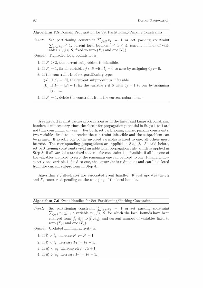
92 Domain Propagation
Algorithm 7.5 Domain Propagation for Set Partitioning/Packing Constraints
Input : Set partitioning constraint∑
j∈S xj = 1 or set packing constraint∑
j∈S xj ≤ 1, current local bounds l ≤ x ≤ u, current number of vari-ables xj , j ∈ S, fixed to zero (F0) and one (F1).
Output : Tightened local bounds for x.
1. If F1 ≥ 2, the current subproblem is infeasible.
2. If F1 = 1, fix all variables j ∈ S with lj = 0 to zero by assigning uj := 0.
3. If the constraint is of set partitioning type:
(a) If F0 = |S|, the current subproblem is infeasible.
(b) If F0 = |S| − 1, fix the variable j ∈ S with uj = 1 to one by assigning
lj := 1.
4. If F1 = 1, delete the constraint from the current subproblem.
A safeguard against useless propagations as in the linear and knapsack constrainthanders is unnecessary, since the checks for propagation potential in Steps 1 to 4 arenot time consuming anyway. For both, set partitioning and set packing constraints,two variables fixed to one render the constraint infeasible and the subproblem canbe pruned. If exactly one of the involved variables is fixed to one, all others mustbe zero. The corresponding propagations are applied in Step 2. As said before,set partitioning constraints yield an additional propagation rule, which is applied inStep 3: if all variables are fixed to zero, the constraint is infeasible; if all but one ofthe variables are fixed to zero, the remaining one can be fixed to one. Finally, if nowexactly one variable is fixed to one, the constraint is redundant and can be deletedfrom the current subproblem in Step 4.
Algorithm 7.6 illustrates the associated event handler. It just updates the F0
and F1 counters depending on the changing of the local bounds.
Algorithm 7.6 Event Handler for Set Partitioning/Packing Constraints
Input : Set partitioning constraint∑
j∈S xj = 1 or set packing constraint∑
j∈S xj ≤ 1, a variable xj , j ∈ S, for which the local bounds have been
changed from [lj , uj ] to [l′j , u′j ], and current number of variables fixed to
zero (F0) and one (F1).
Output : Updated minimal activity α.
1. If l′j > lj , increase F1 := F1 + 1.
2. If l′j < lj , decrease F1 := F1 − 1.
3. If u′j < uj , increase F0 := F0 + 1.
4. If u′j > uj , decrease F0 := F0 − 1.
7.4. Set Covering Constraints 93
7.4 Set Covering Constraints
Set covering constraints are the third type of subset selection constraints, namelythe one that demands that from a set of items at least one has to be selected. It canbe represented as
∑
j∈S
xj ≥ 1
with binary variables xj ∈ {0, 1}, j ∈ S, and S ⊆ I. Again, scaling and complemen-tation may be applied to reach this standard form.
The only propagation rule that can be used for set covering constraints is
∀j ∈ S \ {k} : xj = 0 → xk = 1.
This rule already appeared in Section 7.3 for set partitioning constraints. We treatset covering constraints in a separate section, since their propagation mechanismsubstantially differs from the one used for set partitioning and set packing con-straints. It is specifically tailored to efficiently handle large numbers of constraints.These can, for example, result from the use of conflict analysis, see Chapter 11.
Set covering constraints are equivalent to clauses ℓ1∨ . . .∨ℓ|S| of the satisfiabilityproblem, see Definition 1.3 on page 10. Moskewicz et al. [168] invented a simpleand efficient scheme to propagate SAT clauses, which they called two watched literalsscheme. The main observation is that an implication can be derived from a clauseonly if all but one of the literals are fixed to 0. Thus, a clause only needs to beconsidered for domain propagation after the number of literals fixed to 0 increasedfrom |S| − 2 to |S| − 1. If this is the case, the remaining unfixed literal is impliedand can be fixed to 1.
Instead of using a counter F0 for the number of variables fixed to zero as we didfor the set partitioning and set packing constraints, it suffices for SAT clauses (andthus for set covering constraints) to only watch the state of two arbitrarily chosenliterals of the constraint. As long as both literals remain unfixed, we do not need toprocess the constraint since no propagation can be applied. If one of the watchedliterals is fixed to 0, we inspect the other literals of the clause. If at least one of theother literals is fixed to 1, the constraint is redundant and can be removed from thesubproblem. If at least one of them is unfixed, we stop watching the fixed literaland instead use the unfixed literal as new watched literal. After this switch we haveagain two watched literals, which are unfixed. Finally, if all literals except the otherwatched literal are fixed to 0, the other watched literal is implied and can be fixedto 1.
Moskewicz et al. report a significant speedup for their SAT solver Chaff com-pared to the then state-of-the-art solvers Grasp [157] and Sato [223]. Besidesa different branching rule, the two watched literals scheme is the key element forthe performance improvements of Chaff. The main advantage of this propagationscheme is that—particularly for long clauses—one can simply ignore most of thefixings applied to the involved variables. Despite the inspection of the literals aftera watched literal was fixed to 0, the runtime of the domain propagation procedureis independent from the length of the clause. Another advantage is that we do nothave to perform any bookmarking when the search backtracks to an ancestor of thecurrent node, i.e., a more global subproblem. If the two watched literals are un-fixed in the local subproblem, they remain unfixed in the more global subproblem.If one or both watched literals are fixed in the local subproblem, they will be thefirst literals for which the fixings will be undone on the backtracking path to the
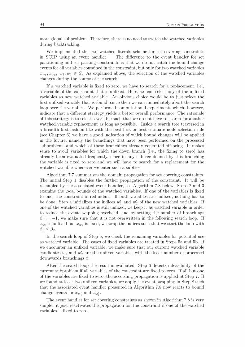
94 Domain Propagation
more global subproblem. Therefore, there is no need to switch the watched variablesduring backtracking.
We implemented the two watched literals scheme for set covering constraintsin SCIP using an event handler. The difference to the event handler for setpartitioning and set packing constraints is that we do not catch the bound changeevents for all variables contained in the constraint, but only for two watched variablesxw1
, xw2, w1, w2 ∈ S. As explained above, the selection of the watched variables
changes during the course of the search.
If a watched variable is fixed to zero, we have to search for a replacement, i.e.,a variable of the constraint that is unfixed. Here, we can select any of the unfixedvariables as new watched variable. An obvious choice would be to just select thefirst unfixed variable that is found, since then we can immediately abort the searchloop over the variables. We performed computational experiments which, however,indicate that a different strategy yields a better overall performance. The rationaleof this strategy is to select a variable such that we do not have to search for anotherwatched variable replacement as long as possible. Inside a search tree traversed ina breadth first fashion like with the best first or best estimate node selection rule(see Chapter 6) we have a good indication of which bound changes will be appliedin the future, namely the branchings that have been performed on the processedsubproblems and which of these branchings already generated offspring. It makessense to avoid variables for which the down branch (i.e., the fixing to zero) hasalready been evaluated frequently, since in any subtree defined by this branchingthe variable is fixed to zero and we will have to search for a replacement for thewatched variable whenever we enter such a subtree.
Algorithm 7.7 summarizes the domain propagation for set covering constraints.The initial Step 1 disables the further propagation of the constraint. It will bereenabled by the associated event handler, see Algorithm 7.8 below. Steps 2 and 3examine the local bounds of the watched variables. If one of the variables is fixedto one, the constraint is redundant. If both variables are unfixed, nothing has tobe done. Step 4 initializes the indices w′1 and w′2 of the new watched variables. Ifone of the watched variables is still unfixed, we keep it as watched variable in orderto reduce the event swapping overhead, and by setting the number of branchingsβi := −1, we make sure that it is not overwritten in the following search loop. Ifxw2
is unfixed but xw1is fixed, we swap the indices such that we start the loop with
β1 ≤ β2.
In the search loop of Step 5, we check the remaining variables for potential useas watched variable. The cases of fixed variables are treated in Steps 5a and 5b. Ifwe encounter an unfixed variable, we make sure that our current watched variablecandidates w′1 and w′2 are the unfixed variables with the least number of processeddownwards branchings β.
After the search loop the result is evaluated. Step 6 detects infeasibility of thecurrent subproblem if all variables of the constraint are fixed to zero. If all but oneof the variables are fixed to zero, the according propagation is applied at Step 7. Ifwe found at least two unfixed variables, we apply the event swapping in Step 8 suchthat the associated event handler presented in Algorithm 7.8 now reacts to boundchange events for xw′
1and xw′
2.
The event handler for set covering constraints as shown in Algorithm 7.8 is verysimple: it just reactivates the propagation for the constraint if one of the watchedvariables is fixed to zero.
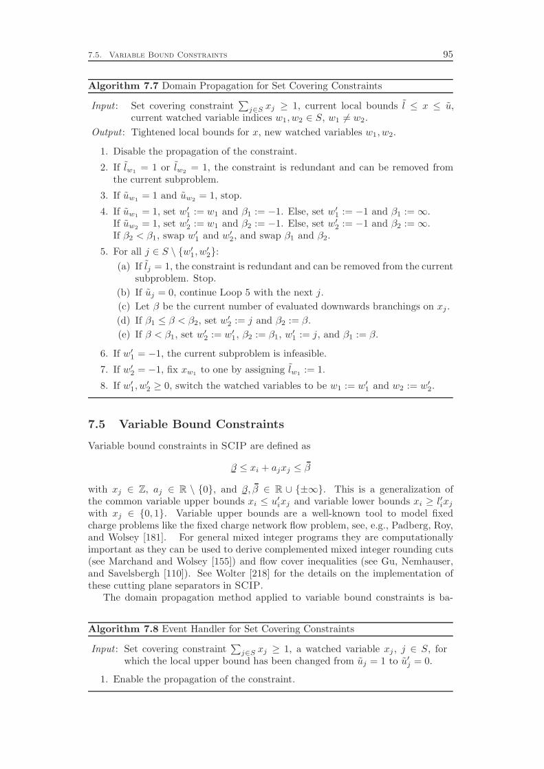
7.5. Variable Bound Constraints 95
Algorithm 7.7 Domain Propagation for Set Covering Constraints
Input : Set covering constraint∑
j∈S xj ≥ 1, current local bounds l ≤ x ≤ u,current watched variable indices w1, w2 ∈ S, w1 6= w2.
Output : Tightened local bounds for x, new watched variables w1, w2.
1. Disable the propagation of the constraint.
2. If lw1= 1 or lw2
= 1, the constraint is redundant and can be removed fromthe current subproblem.
3. If uw1= 1 and uw2
= 1, stop.
4. If uw1= 1, set w′1 := w1 and β1 := −1. Else, set w′1 := −1 and β1 :=∞.
If uw2= 1, set w′2 := w1 and β2 := −1. Else, set w′2 := −1 and β2 :=∞.
If β2 < β1, swap w′1 and w′2, and swap β1 and β2.
5. For all j ∈ S \ {w′1, w′2}:
(a) If lj = 1, the constraint is redundant and can be removed from the currentsubproblem. Stop.
(b) If uj = 0, continue Loop 5 with the next j.
(c) Let β be the current number of evaluated downwards branchings on xj .
(d) If β1 ≤ β < β2, set w′2 := j and β2 := β.
(e) If β < β1, set w′2 := w′1, β2 := β1, w′1 := j, and β1 := β.
6. If w′1 = −1, the current subproblem is infeasible.
7. If w′2 = −1, fix xw1to one by assigning lw1
:= 1.
8. If w′1, w′2 ≥ 0, switch the watched variables to be w1 := w′1 and w2 := w′2.
7.5 Variable Bound Constraints
Variable bound constraints in SCIP are defined as
β ≤ xi + ajxj ≤ β
with xj ∈ Z, aj ∈ R \ {0}, and β, β ∈ R ∪ {±∞}. This is a generalization ofthe common variable upper bounds xi ≤ u′ixj and variable lower bounds xi ≥ l′ixj
with xj ∈ {0, 1}. Variable upper bounds are a well-known tool to model fixedcharge problems like the fixed charge network flow problem, see, e.g., Padberg, Roy,and Wolsey [181]. For general mixed integer programs they are computationallyimportant as they can be used to derive complemented mixed integer rounding cuts(see Marchand and Wolsey [155]) and flow cover inequalities (see Gu, Nemhauser,and Savelsbergh [110]). See Wolter [218] for the details on the implementation ofthese cutting plane separators in SCIP.
The domain propagation method applied to variable bound constraints is ba-
Algorithm 7.8 Event Handler for Set Covering Constraints
Input : Set covering constraint∑
j∈S xj ≥ 1, a watched variable xj , j ∈ S, forwhich the local upper bound has been changed from uj = 1 to u′j = 0.
1. Enable the propagation of the constraint.

96 Domain Propagation
sically the same as for the general linear constraints of Section 7.1. As for thepreviously described specializations of linear constraints, the advantage of an indi-vidual constraint handler for variable bound constraints is the possibility of a morecompact data representation and an easier and faster propagation method.
The following propagations are applied:
xi ≥ β − ajuj for aj > 0 and xi ≥ β − aj lj for aj < 0, (7.5)
xi ≤ β − aj lj for aj > 0 and xi ≤ β − aj uj for aj < 0, (7.6)
xj ≥⌈β − ui
aj
⌉
for aj > 0 and xj ≤⌊β − ui
aj
⌋
for aj < 0, (7.7)
xj ≤⌊β − li
aj
⌋
for aj > 0 and xj ≥⌈β − li
aj
⌉
for aj < 0. (7.8)
Since these calculations are not as involved as the ones for general linear constraints,we do not need to apply a conservative rounding as in Equation (7.2) on page 86 forthe propagation of linear constraints. However, the risk of numerous iterated smalltightenings of domains of general integer or continuous variables is also presentfor variable bound constraints. Therefore, we use the same limits on the minimalfraction to cut off from domains as for linear constraints, see Inequalities (7.3).
Algorithm 7.9 recapitulates the propagation procedure for variable bound con-straints. As for linear constraints, a propagation mark controls whether the con-straint has to be considered again for propagation. This mark is reset by the asso-ciated event handler as can be seen in Algorithm 7.10.
7.6 Objective Propagation
The propagations described in the previous sections are based on primal feasibilityreasoning: a bound is tightened because setting a variable to a value outside thetightened bounds leads to an infeasible subproblem. The objective propagation ofthis section and the root reduced cost strengthening of the following section take thedual point of view. They infer bounds that are valid due to optimality considerations:if the variable takes a value outside the tightened bounds, the solution cannot bebetter than the current incumbent.
Let c = cT x be the objective value of the current incumbent solution x ∈ Rn, i.e.,the smallest objective value of all feasible solutions found so far. Then, the objectivefunction can be used to rule out inferior solutions by propagating
∑
j∈N
cjxj ≤ c− δ (7.9)
with δ ∈ R>0 being the dual feasibility tolerance or optimality tolerance. Thisobjective constraint is a regular linear constraint, and we can use Algorithm 7.1 topropagate it.
The objective cutoff, i.e., the right hand side c of Inequality (7.9), can be tightenedif the objective function value is always integral. A sufficient condition for objectiveintegrality is that
⊲ all objective coefficients are integral: cj ∈ Z for all j ∈ N , and
⊲ all objective coefficients for continuous variables are zero: cj = 0 for all j ∈ C.
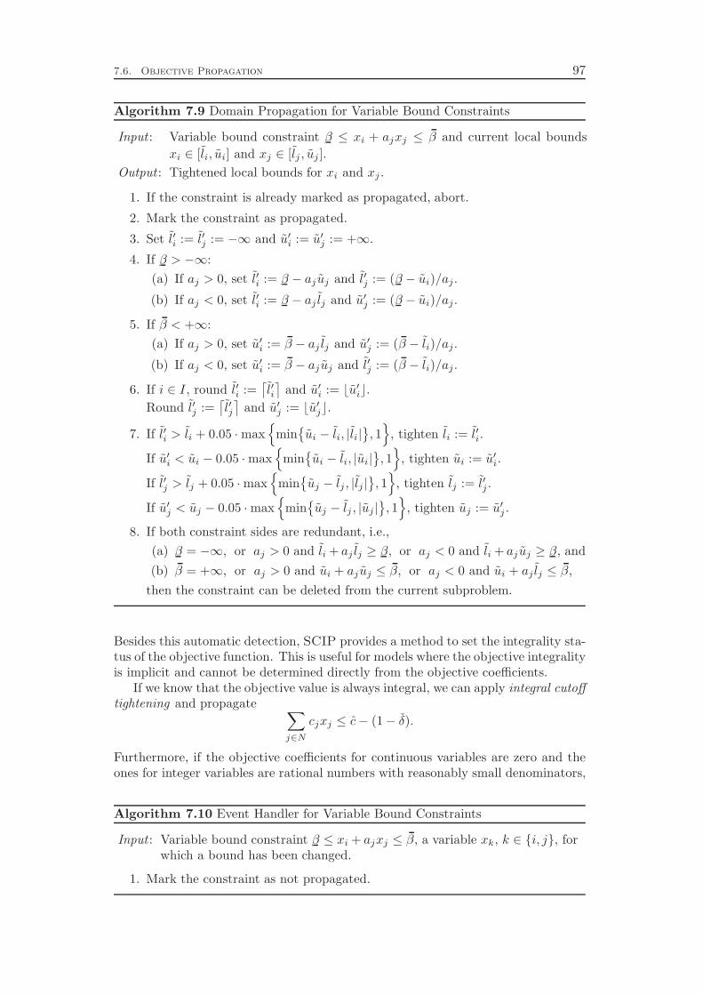
7.6. Objective Propagation 97
Algorithm 7.9 Domain Propagation for Variable Bound Constraints
Input : Variable bound constraint β ≤ xi + ajxj ≤ β and current local bounds
xi ∈ [li, ui] and xj ∈ [lj , uj ].
Output : Tightened local bounds for xi and xj .
1. If the constraint is already marked as propagated, abort.
2. Mark the constraint as propagated.
3. Set l′i := l′j := −∞ and u′i := u′j := +∞.
4. If β > −∞:
(a) If aj > 0, set l′i := β − aj uj and l′j := (β − ui)/aj .
(b) If aj < 0, set l′i := β − aj lj and u′j := (β − ui)/aj .
5. If β < +∞:
(a) If aj > 0, set u′i := β − aj lj and u′j := (β − li)/aj .
(b) If aj < 0, set u′i := β − aj uj and l′j := (β − li)/aj .
6. If i ∈ I, round l′i :=⌈l′i⌉
and u′i := ⌊u′i⌋.
Round l′j :=⌈l′j⌉
and u′j := ⌊u′j⌋.
7. If l′i > li + 0.05 ·max{
min{ui − li, |li|
}, 1}
, tighten li := l′i.
If u′i < ui − 0.05 ·max{
min{ui − li, |ui|
}, 1}
, tighten ui := u′i.
If l′j > lj + 0.05 ·max{
min{uj − lj , |lj |
}, 1}
, tighten lj := l′j .
If u′j < uj − 0.05 ·max{
min{uj − lj , |uj |
}, 1}
, tighten uj := u′j .
8. If both constraint sides are redundant, i.e.,
(a) β = −∞, or aj > 0 and li + aj lj ≥ β, or aj < 0 and li + aj uj ≥ β, and
(b) β = +∞, or aj > 0 and ui + aj uj ≤ β, or aj < 0 and ui + aj lj ≤ β,
then the constraint can be deleted from the current subproblem.
Besides this automatic detection, SCIP provides a method to set the integrality sta-tus of the objective function. This is useful for models where the objective integralityis implicit and cannot be determined directly from the objective coefficients.
If we know that the objective value is always integral, we can apply integral cutofftightening and propagate
∑
j∈N
cjxj ≤ c− (1− δ).
Furthermore, if the objective coefficients for continuous variables are zero and theones for integer variables are rational numbers with reasonably small denominators,
Algorithm 7.10 Event Handler for Variable Bound Constraints
Input : Variable bound constraint β ≤ xi + ajxj ≤ β, a variable xk, k ∈ {i, j}, forwhich a bound has been changed.
1. Mark the constraint as not propagated.
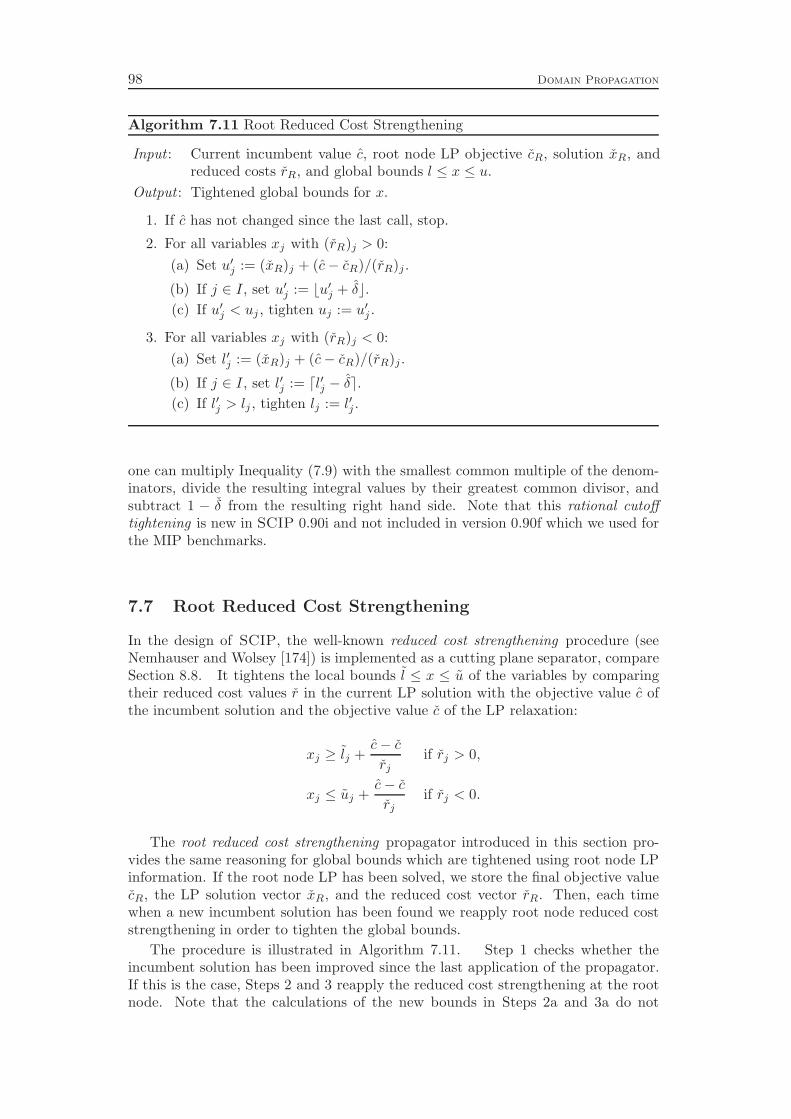
98 Domain Propagation
Algorithm 7.11 Root Reduced Cost Strengthening
Input : Current incumbent value c, root node LP objective cR, solution xR, andreduced costs rR, and global bounds l ≤ x ≤ u.
Output : Tightened global bounds for x.
1. If c has not changed since the last call, stop.
2. For all variables xj with (rR)j > 0:
(a) Set u′j := (xR)j + (c− cR)/(rR)j .
(b) If j ∈ I, set u′j := ⌊u′j + δ⌋.
(c) If u′j < uj , tighten uj := u′j .
3. For all variables xj with (rR)j < 0:
(a) Set l′j := (xR)j + (c− cR)/(rR)j .
(b) If j ∈ I, set l′j := ⌈l′j − δ⌉.
(c) If l′j > lj , tighten lj := l′j .
one can multiply Inequality (7.9) with the smallest common multiple of the denom-inators, divide the resulting integral values by their greatest common divisor, andsubtract 1 − δ from the resulting right hand side. Note that this rational cutofftightening is new in SCIP 0.90i and not included in version 0.90f which we used forthe MIP benchmarks.
7.7 Root Reduced Cost Strengthening
In the design of SCIP, the well-known reduced cost strengthening procedure (seeNemhauser and Wolsey [174]) is implemented as a cutting plane separator, compareSection 8.8. It tightens the local bounds l ≤ x ≤ u of the variables by comparingtheir reduced cost values r in the current LP solution with the objective value c ofthe incumbent solution and the objective value c of the LP relaxation:
xj ≥ lj +c− c
rjif rj > 0,
xj ≤ uj +c− c
rjif rj < 0.
The root reduced cost strengthening propagator introduced in this section pro-vides the same reasoning for global bounds which are tightened using root node LPinformation. If the root node LP has been solved, we store the final objective valuecR, the LP solution vector xR, and the reduced cost vector rR. Then, each timewhen a new incumbent solution has been found we reapply root node reduced coststrengthening in order to tighten the global bounds.
The procedure is illustrated in Algorithm 7.11. Step 1 checks whether theincumbent solution has been improved since the last application of the propagator.If this is the case, Steps 2 and 3 reapply the reduced cost strengthening at the rootnode. Note that the calculations of the new bounds in Steps 2a and 3a do not
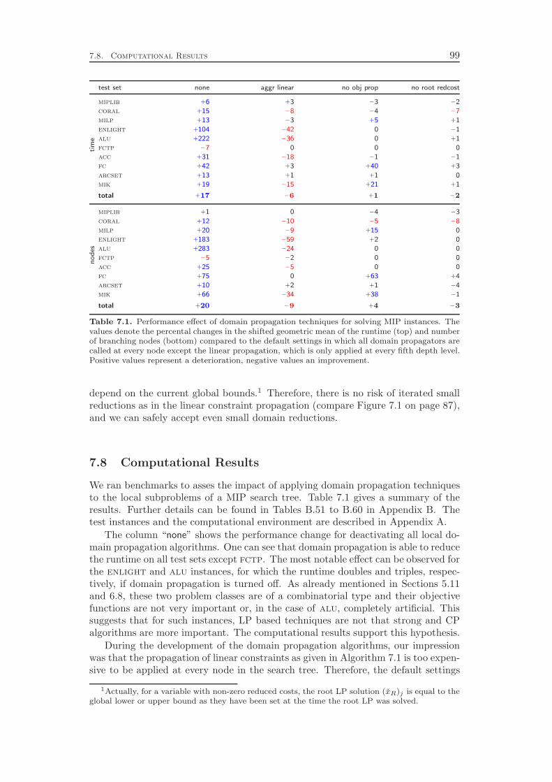
7.8. Computational Results 99
test set none aggr linear no obj prop no root redcostti
me
miplib +6 +3 −3 −2
coral +15 −8 −4 −7
milp +13 −3 +5 +1
enlight +104 −42 0 −1
alu +222 −36 0 +1
fctp −7 0 0 0
acc +31 −18 −1 −1
fc +42 +3 +40 +3
arcset +13 +1 +1 0
mik +19 −15 +21 +1
total +17 −6 +1 −2
no
des
miplib +1 0 −4 −3
coral +12 −10 −5 −8
milp +20 −9 +15 0
enlight +183 −59 +2 0
alu +283 −24 0 0
fctp −5 −2 0 0
acc +25 −5 0 0
fc +75 0 +63 +4
arcset +10 +2 +1 −4
mik +66 −34 +38 −1
total +20 −9 +4 −3
Table 7.1. Performance effect of domain propagation techniques for solving MIP instances. Thevalues denote the percental changes in the shifted geometric mean of the runtime (top) and numberof branching nodes (bottom) compared to the default settings in which all domain propagators arecalled at every node except the linear propagation, which is only applied at every fifth depth level.Positive values represent a deterioration, negative values an improvement.
depend on the current global bounds.1 Therefore, there is no risk of iterated smallreductions as in the linear constraint propagation (compare Figure 7.1 on page 87),and we can safely accept even small domain reductions.
7.8 Computational Results
We ran benchmarks to asses the impact of applying domain propagation techniquesto the local subproblems of a MIP search tree. Table 7.1 gives a summary of theresults. Further details can be found in Tables B.51 to B.60 in Appendix B. Thetest instances and the computational environment are described in Appendix A.
The column “none” shows the performance change for deactivating all local do-main propagation algorithms. One can see that domain propagation is able to reducethe runtime on all test sets except fctp. The most notable effect can be observed forthe enlight and alu instances, for which the runtime doubles and triples, respec-tively, if domain propagation is turned off. As already mentioned in Sections 5.11and 6.8, these two problem classes are of a combinatorial type and their objectivefunctions are not very important or, in the case of alu, completely artificial. Thissuggests that for such instances, LP based techniques are not that strong and CPalgorithms are more important. The computational results support this hypothesis.
During the development of the domain propagation algorithms, our impressionwas that the propagation of linear constraints as given in Algorithm 7.1 is too expen-sive to be applied at every node in the search tree. Therefore, the default settings
1Actually, for a variable with non-zero reduced costs, the root LP solution (xR)j is equal to theglobal lower or upper bound as they have been set at the time the root LP was solved.

100 Domain Propagation
are to invoke the algorithm only at every fifth depth level. The column “aggr linear”shows the effect of applying the linear domain propagation at every node. It turnsout that our concerns are unjustified: applying linear domain propagation at everynode improves the performance on almost all test sets. Again, the largest speedupcan be observed on the enlight and alu instances.
The columns “no obj prop” and “no root redcost” demonstrate the impact ofthe two dual propagation methods included in SCIP. Both techniques have onlya very small effect. However, the objective propagation considerably improves theperformance on the fc and mik test sets. As can be seen in Table B.58, the runtimeincreases by at least 10 % for 13 out of the 20 fc instances if objective propagationis disabled. In contrast, not a single instance in this test set can be solved fasterwithout objective propagation.
Chapter 8
Cut Separation
Cutting planes for integer and mixed integer programming have been studied sincethe late 1950’s. One of the most fundamental work in this area has been conductedby Gomory [102, 103, 104] who proved that integer programs with rational data canbe solved in a finite number of steps by a pure cutting plane approach without anybranching. Unfortunately, numerical issues in Gomory’s approach prevented purecutting plane methods from being effective in practice.
With the work of Balas et al. [31] in 1996 and finally with the release of Cplex 6.5in 1999, it became clear that cutting planes, in particular Gomory mixed integercuts, are very efficient if combined with branch-and-bound. The resulting algorithmis called cut-and-branch or branch-and-cut, depending on whether cutting planes areonly generated at the root node or also at local subproblems in the search tree, seeSection 2.2. Bixby et al. [46] report a speed-up of a factor of 22.3 from Cplex 6.0to Cplex 6.5, with cutting planes providing a major contribution to this success.
Since the theory of cutting planes is very well covered in the literature (see, e.g.,a recent survey by Klar [132]), this chapter focuses on the cutting plane separationmethods that are available in SCIP. We will, however, only briefly sketch the al-gorithms and the underlying theory. A detailed description, including the theoryand computational experiments that compare various SCIP parameter settings anddifferent implementations, can be found in the diploma thesis of Wolter [218]. Addi-tional information about computationally important cutting planes can, for example,be found in Marchand et al. [154] and in Fügenschuh and Martin [90].
Some of the results presented here, namely the sections about knapsack covercuts, mixed integer rounding cuts, strong Chvátal-Gomory cuts, implied bound cuts,and clique cuts are joint work with Kati Wolter. The implementation of Gomorymixed integer cuts, knapsack cover cuts, and reduced cost strengthening is basedon Alexander Martin’s implementation of SIP [159]. The SCIP algorithms for flowcover cuts have been implemented by Kati Wolter.
8.1 Knapsack Cover Cuts
The knapsack polytope is one of the most thoroughly studied polyhedrons in mathe-matical programming, see for instance Balas [28], Hammer, Johnson, and Peled [112],Padberg [179, 180], Wolsey [216], Balas and Zemel [35, 36], Weismantel [212], or Mar-tin and Weismantel [160]. Knapsack cover cuts, which are a particular family of validinequalities for the knapsack polytope, are probably one of the first cutting planesthat have been incorporated into commercial MIP solvers. For example, they areavailable in Cplex since version 3.0. Crowder, Johnson, and Padberg [70] were thefirst to successfully apply lifted knapsack cover inequalities to solve several binaryprograms that were, at the time, considered to be intractable.
In its most basic version, the knapsack cover cut can be derived as follows.
101
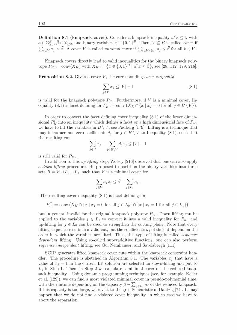
102 Cut Separation
Definition 8.1 (knapsack cover). Consider a knapsack inequality aTx ≤ β witha ∈ ZB
≥0, β ∈ Z≥0, and binary variables x ∈ {0, 1}B . Then, V ⊆ B is called cover if∑
j∈V aj > β. A cover V is called minimal cover if∑
j∈V \{k} aj ≤ β for all k ∈ V .
Knapsack covers directly lead to valid inequalities for the binary knapsack poly-tope PK := conv(XK) with XK :=
{x ∈ {0, 1}B | aTx ≤ β
}, see [28, 112, 179, 216]:
Proposition 8.2. Given a cover V , the corresponding cover inequality
∑
j∈V
xj ≤ |V | − 1 (8.1)
is valid for the knapsack polytope PK . Furthermore, if V is a minimal cover, In-equality (8.1) is facet defining for P ′K := conv
(XK ∩ {x | xj = 0 for all j ∈ B \V }
).
In order to convert the facet defining cover inequality (8.1) of the lower dimen-sional P ′K into an inequality which defines a facet or a high dimensional face of PK ,we have to lift the variables in B \ V , see Padberg [179]. Lifting is a technique thatmay introduce non-zero coefficients dj for j ∈ B \ V to Inequality (8.1), such thatthe resulting cut
∑
j∈V
xj +∑
j∈B\V
djxj ≤ |V | − 1
is still valid for PK .In addition to this up-lifting step, Wolsey [216] observed that one can also apply
a down-lifting procedure. He proposed to partition the binary variables into threesets B = V ∪ L0 ∪ L1, such that V is a minimal cover for
∑
j∈V
ajxj ≤ β −∑
j∈L1
aj .
The resulting cover inequality (8.1) is facet defining for
P ′′K := conv(XK ∩ {x | xj = 0 for all j ∈ L0} ∩ {x | xj = 1 for all j ∈ L1}
),
but in general invalid for the original knapsack polytope PK . Down-lifting can beapplied to the variables j ∈ L1 to convert it into a valid inequality for PK , andup-lifting for j ∈ L0 can be used to strengthen the cutting plane. Note that everylifting sequence results in a valid cut, but the coefficients dj of the cut depend on theorder in which the variables are lifted. Thus, this type of lifting is called sequencedependent lifting. Using so-called superadditive functions, one can also performsequence independent lifting, see Gu, Nemhauser, and Savelsbergh [111].
SCIP generates lifted knapsack cover cuts within the knapsack constraint han-dler. The procedure is sketched in Algorithm 8.1. The variables xj that have avalue of xj = 1 in the current LP solution are selected for down-lifting and put toL1 in Step 1. Then, in Step 2 we calculate a minimal cover on the reduced knap-sack inequality. Using dynamic programming techniques (see, for example, Kelleret al. [129]), we can find a most violated minimal cover in pseudo-polynomial time,with the runtime depending on the capacity β −
∑
j∈L1aj of the reduced knapsack.
If this capacity is too large, we revert to the greedy heuristic of Dantzig [74]. It mayhappen that we do not find a violated cover inequality, in which case we have toabort the separation.
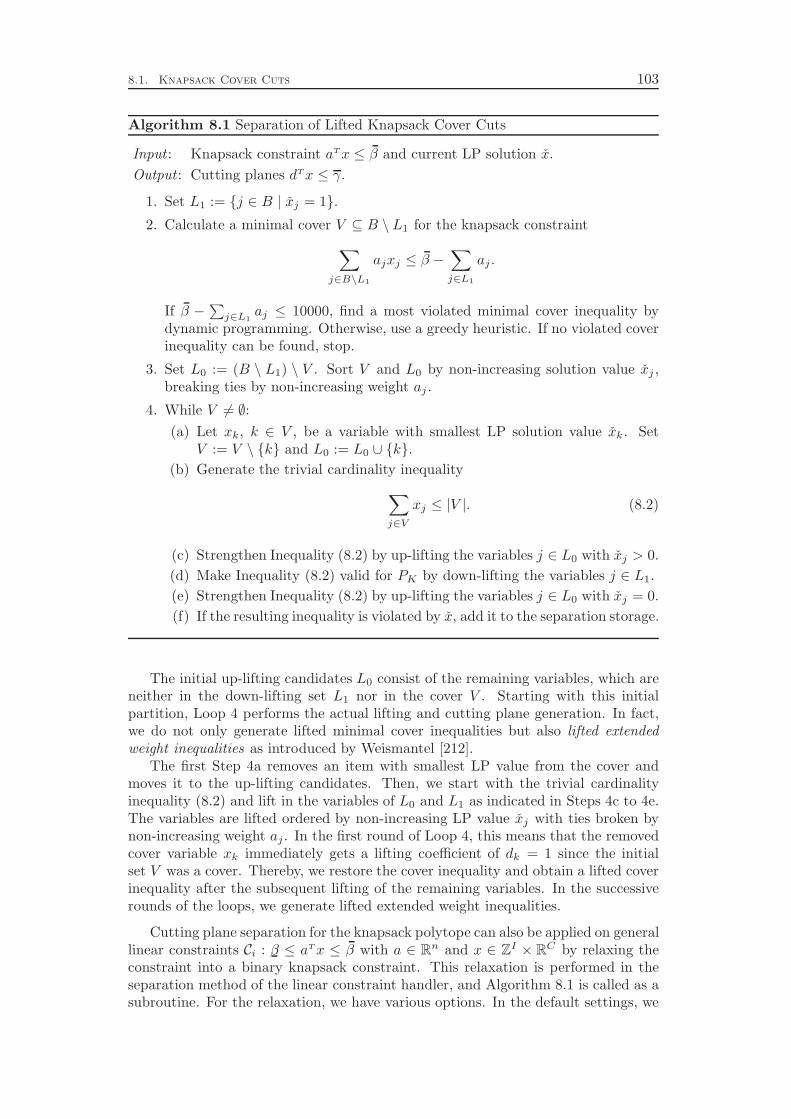
8.1. Knapsack Cover Cuts 103
Algorithm 8.1 Separation of Lifted Knapsack Cover Cuts
Input : Knapsack constraint aTx ≤ β and current LP solution x.
Output : Cutting planes dTx ≤ γ.
1. Set L1 := {j ∈ B | xj = 1}.
2. Calculate a minimal cover V ⊆ B \ L1 for the knapsack constraint
∑
j∈B\L1
ajxj ≤ β −∑
j∈L1
aj .
If β −∑
j∈L1aj ≤ 10000, find a most violated minimal cover inequality by
dynamic programming. Otherwise, use a greedy heuristic. If no violated coverinequality can be found, stop.
3. Set L0 := (B \ L1) \ V . Sort V and L0 by non-increasing solution value xj ,breaking ties by non-increasing weight aj .
4. While V 6= ∅:
(a) Let xk, k ∈ V , be a variable with smallest LP solution value xk. SetV := V \ {k} and L0 := L0 ∪ {k}.
(b) Generate the trivial cardinality inequality
∑
j∈V
xj ≤ |V |. (8.2)
(c) Strengthen Inequality (8.2) by up-lifting the variables j ∈ L0 with xj > 0.
(d) Make Inequality (8.2) valid for PK by down-lifting the variables j ∈ L1.
(e) Strengthen Inequality (8.2) by up-lifting the variables j ∈ L0 with xj = 0.
(f) If the resulting inequality is violated by x, add it to the separation storage.
The initial up-lifting candidates L0 consist of the remaining variables, which areneither in the down-lifting set L1 nor in the cover V . Starting with this initialpartition, Loop 4 performs the actual lifting and cutting plane generation. In fact,we do not only generate lifted minimal cover inequalities but also lifted extendedweight inequalities as introduced by Weismantel [212].
The first Step 4a removes an item with smallest LP value from the cover andmoves it to the up-lifting candidates. Then, we start with the trivial cardinalityinequality (8.2) and lift in the variables of L0 and L1 as indicated in Steps 4c to 4e.The variables are lifted ordered by non-increasing LP value xj with ties broken bynon-increasing weight aj . In the first round of Loop 4, this means that the removedcover variable xk immediately gets a lifting coefficient of dk = 1 since the initialset V was a cover. Thereby, we restore the cover inequality and obtain a lifted coverinequality after the subsequent lifting of the remaining variables. In the successiverounds of the loops, we generate lifted extended weight inequalities.
Cutting plane separation for the knapsack polytope can also be applied on generallinear constraints Ci : β ≤ aTx ≤ β with a ∈ Rn and x ∈ ZI × RC by relaxing theconstraint into a binary knapsack constraint. This relaxation is performed in theseparation method of the linear constraint handler, and Algorithm 8.1 is called as asubroutine. For the relaxation, we have various options. In the default settings, we
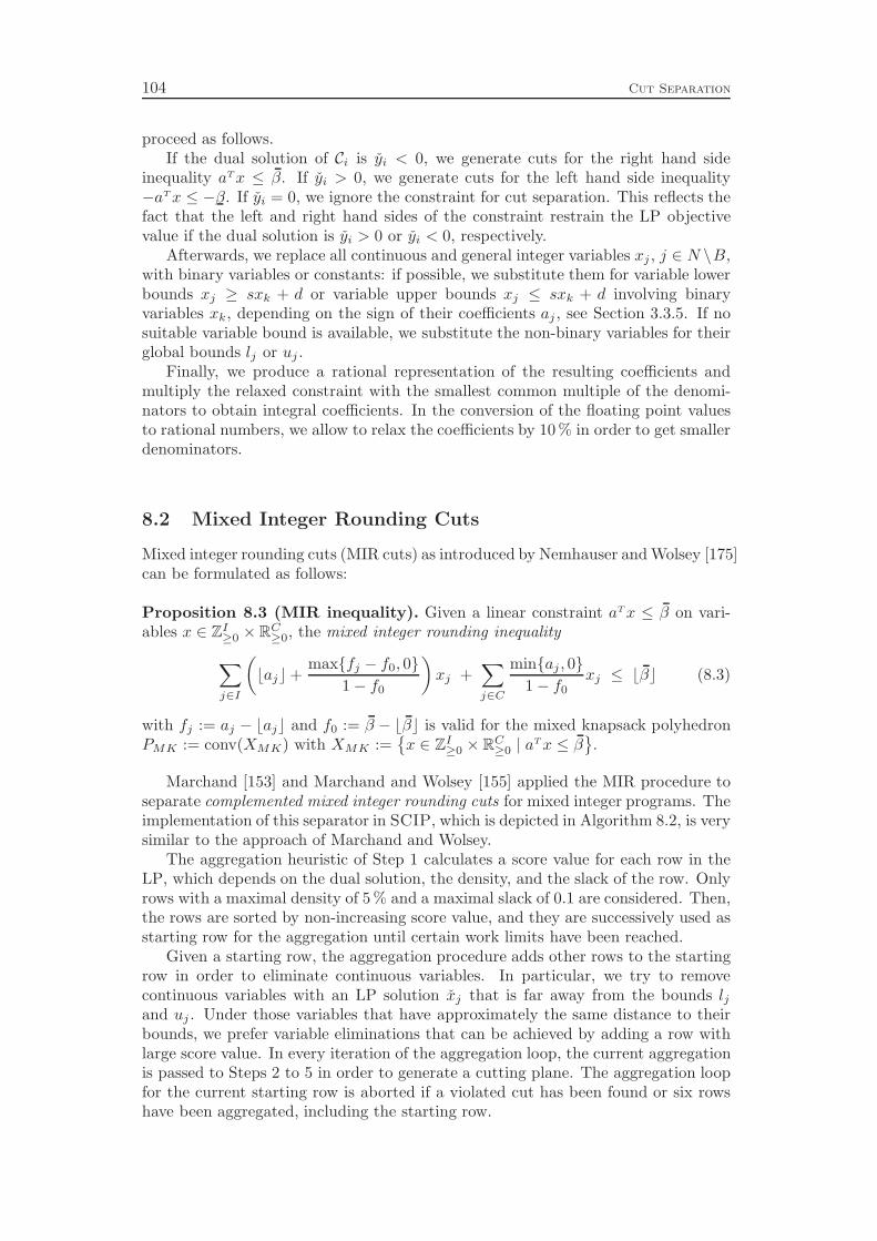
104 Cut Separation
proceed as follows.If the dual solution of Ci is yi < 0, we generate cuts for the right hand side
inequality aTx ≤ β. If yi > 0, we generate cuts for the left hand side inequality−aTx ≤ −β. If yi = 0, we ignore the constraint for cut separation. This reflects thefact that the left and right hand sides of the constraint restrain the LP objectivevalue if the dual solution is yi > 0 or yi < 0, respectively.
Afterwards, we replace all continuous and general integer variables xj , j ∈ N \B,with binary variables or constants: if possible, we substitute them for variable lowerbounds xj ≥ sxk + d or variable upper bounds xj ≤ sxk + d involving binaryvariables xk, depending on the sign of their coefficients aj , see Section 3.3.5. If nosuitable variable bound is available, we substitute the non-binary variables for theirglobal bounds lj or uj .
Finally, we produce a rational representation of the resulting coefficients andmultiply the relaxed constraint with the smallest common multiple of the denomi-nators to obtain integral coefficients. In the conversion of the floating point valuesto rational numbers, we allow to relax the coefficients by 10 % in order to get smallerdenominators.
8.2 Mixed Integer Rounding Cuts
Mixed integer rounding cuts (MIR cuts) as introduced by Nemhauser and Wolsey [175]can be formulated as follows:
Proposition 8.3 (MIR inequality). Given a linear constraint aTx ≤ β on vari-ables x ∈ ZI
≥0 × RC≥0, the mixed integer rounding inequality
∑
j∈I
(
⌊aj⌋+max{fj − f0, 0}
1− f0
)
xj +∑
j∈C
min{aj , 0}
1− f0xj ≤ ⌊β⌋ (8.3)
with fj := aj − ⌊aj⌋ and f0 := β − ⌊β⌋ is valid for the mixed knapsack polyhedronPMK := conv(XMK) with XMK :=
{x ∈ ZI
≥0 × RC≥0 | a
Tx ≤ β}
.
Marchand [153] and Marchand and Wolsey [155] applied the MIR procedure toseparate complemented mixed integer rounding cuts for mixed integer programs. Theimplementation of this separator in SCIP, which is depicted in Algorithm 8.2, is verysimilar to the approach of Marchand and Wolsey.
The aggregation heuristic of Step 1 calculates a score value for each row in theLP, which depends on the dual solution, the density, and the slack of the row. Onlyrows with a maximal density of 5 % and a maximal slack of 0.1 are considered. Then,the rows are sorted by non-increasing score value, and they are successively used asstarting row for the aggregation until certain work limits have been reached.
Given a starting row, the aggregation procedure adds other rows to the startingrow in order to eliminate continuous variables. In particular, we try to removecontinuous variables with an LP solution xj that is far away from the bounds ljand uj . Under those variables that have approximately the same distance to theirbounds, we prefer variable eliminations that can be achieved by adding a row withlarge score value. In every iteration of the aggregation loop, the current aggregationis passed to Steps 2 to 5 in order to generate a cutting plane. The aggregation loopfor the current starting row is aborted if a violated cut has been found or six rowshave been aggregated, including the starting row.
8.3. Gomory Mixed Integer Cuts 105
Algorithm 8.2 Separation of Complemented MIR Cuts
Input : LP relaxation Ax ≤ b of MIP, global bounds l ≤ x ≤ u, and current LPsolution x.
Output : Cutting planes dTx ≤ γ.
1. Aggregate linear constraints to obtain a single linear inequality aTx ≤ β.
2. Transform the variables to the canonical form x′ ≥ 0 by either
⊲ shifting to their lower bound xj ≥ lj : x′j := xj − lj ,
⊲ complementing to their upper bound xj ≤ uj : x′j := uj − xj ,
⊲ substituting with a variable lower bound xj ≥ sxk + d, k ∈ I:x′j := xj − (sxk + d), or
⊲ substituting with a variable upper bound xj ≤ sxk + d, k ∈ I:x′j := (sxk + d)− xj .
3. Divide the resulting inequality a′Tx′ ≤ β′ by δ = ±1, δ = ±max{|a′j | | j ∈ I},and δ ∈ {±a′j | j ∈ I and 0 < x′j < u′j}, and generate the corresponding MIRinequalities (8.3). Choose δ⋆ to be the δ for which the most violated MIRinequality has been produced.
4. In addition to δ⋆, check whether the MIR inequalities derived from dividinga′Tx′ ≤ β′ by 1
2δ⋆, 1
4δ⋆, and 1
8δ⋆ yield even larger violations.
5. Finally, select the most violated of the MIR inequalities, transform it back intothe space of problem variables x, substitute slack variables, and add it to theseparation storage.
The bound substitution in Step 2 always selects the bound that is closest to thecurrent LP solution xj . If the LP value of a variable bound is at least as close asthe global bound, we prefer variable bounds over global bounds.
Marchand and Wolsey [155] propose to augment the cutting plane separationprocedure with a final step of additional variable complementation in order to findan even more violated cut. This complementation would be performed after Step 4.We do not follow this approach, since it turned out to be inferior in early benchmarktests. Instead, we slightly extend the bound substitution heuristic of Step 2: if theresulting right hand side β′ is integral, we complement one additional variable oruncomplement one of the complemented variables to obtain a fractional right handside.
8.3 Gomory Mixed Integer Cuts
Besides lift-and-project cuts (see Balas, Ceria, and Cornuéjols [29, 30]), Gomorymixed integer cuts (GMI cuts) have been the first general purpose cutting planesthat were successfully employed within a branch-and-cut framework to solve mixedinteger programs, see Balas et al. [31]. They have been discovered by Gomory [103,104] in 1960, but despite their theoretical value, namely providing a method to solveinteger programs with rational data, they have been regarded as computationallyuseless. This reputation changed with the work of Balas et al., and nowadays GMI

106 Cut Separation
cuts seem to be one of the most important cutting planes employed in mixed integersolvers, see Bixby et al. [46].
Gomory mixed integer cuts can be stated as follows [103, 31]:
Proposition 8.4 (Gomory mixed integer cuts). Let B ⊆ N be an optimalsimplex basis for the LP relaxation of a MIP in equality form
c⋆ = min{cTx | Ax = b, x ≥ 0, xj ∈ Z for all j ∈ I ⊆ N},
and let N := N \ B denote the index set of non-basic variables. Furthermore, leta = (A−1
B A)i · be row i of the simplex tableau, a0 = (A−1B b)i be the right hand side
of this tableau row, and fj = aj − ⌊aj⌋ be the fractional parts of the tableau rowentries, j ∈ N ∪{0}. Then, if xi, i ∈ B∩ I, is a basic integer variable with fractionalLP solution xi = a0 /∈ Z, the Gomory mixed integer cut
∑
j∈N∩I
min{fj
f0,1− fj
1− f0
}
xj +∑
j∈N∩C
max{ aj
f0,−aj
1− f0
}
xj ≥ 1 (8.4)
is valid for the MIP and cuts off the fractional LP solution x.
The following proposition shows that GMI cuts are a subclass of MIR cuts andcan be derived by employing the MIR procedure of Proposition 8.3 to the simplextableau equation.
Proposition 8.5. The Gomory mixed integer cut (8.4) is equivalent to the mixedinteger rounding cut (8.3) applied to the simplex tableau row
xi +∑
j∈N
ajxj = a0 (8.5)
for a non-basic integer variable xi, i ∈ N ∩ I, with fractional a0 /∈ Z.
Proof. Multiplying the GMI cut (8.4) by −f0 yields the equivalent constraint
∑
j∈N∩I
max{
−fj ,−f01− fj
1− f0
}
xj +∑
j∈N∩C
min{
−aj ,ajf0
1− f0
}
xj ≤ −f0. (8.6)
Adding Inequality (8.6) to the feasible Equation (8.5) yields
xi +∑
j∈N∩I
max{
aj−fj , aj−f01− fj
1− f0
}
xj +∑
j∈N∩C
min{
0, aj +ajf0
1− f0
}
xj ≤ a0−f0,
which is equivalent to
xi +∑
j∈N∩I
(
⌊aj⌋+ max{
0,fj − f01− f0
})
xj +∑
j∈N∩C
min{
0,aj
1− f0
}
xj ≤ ⌊a0⌋.
This final inequality is exactly same as the MIR cut for the tableau row (8.5) in thedirection xi +
∑
j∈N ajxj ≤ a0.
Following Proposition 8.5, the Gomory mixed integer cut separator of SCIPjust applies Steps 1, 2, and 5 of the c-MIR cut separation Algorithm 8.2. For eachfractional integer basic variable xi, the aggregation of Step 1 is performed using theweights given by the corresponding row (A−1
B )i · in the basis inverse, such that theaggregation produces Equation 8.5, which may include slack variables. The boundsubstitution of Step 2 only complements those variables that are at their upperbounds.
8.4. Strong Chvátal-Gomory Cuts 107
8.4 Strong Chvátal-Gomory Cuts
Letchford and Lodi [142] proposed a method to strengthen Chvátal-Gomory cuts [60],which are closely related to Gomory fractional cuts [102]. Given a linear inequalityaTx ≤ β on non-negative integer variables xj ∈ Z≥0, j ∈ I = N , the Chvátal-Gomory cut (CG cut) can be derived by rounding down the coefficient vector andthe right hand side:
∑
j∈I
⌊aj⌋x ≤ ⌊β⌋. (8.7)
It is easy to see that this inequality is valid, since after rounding down the coefficientsof the inequality the activity is always integral, which also allows for rounding downthe right hand side. One way to obtain a stronger cut is to instead apply the mixedinteger rounding procedure given in Inequality (8.3). The MIR cut always dominatesthe CG cut, since their right hand sides are equal and the coefficients of the MIRcut are greater or equal to the coefficients of the CG cut. Additionally, the MIRprocedure can be applied to constraints that include continuous variables.
Letchford and Lodi suggest a different strengthening of the CG cut for inequalitiescontaining only integer variables, which is given by the following theorem [142]:
Theorem 8.6 (strong Chvátal-Gomory cut). Consider the inequality aTx ≤ βon non-negative integer variables xj ∈ Z≥0, j ∈ I = N . Suppose that f0 = β−⌊β⌋ >0 and let k ≥ 1 be the unique integer such that 1
k+1 ≤ f0 <1k
. Partition N intoclasses N0, . . . ,Nk as follows. Let N0 = {j ∈ N | fj ≤ f0} and, for p = 1, . . . , k, letNp = {j ∈ N | f0 + 1
k(p− 1)(1− f0) < fj ≤ f0 + 1
kp(1− f0)}. The inequality
k∑
p=0
∑
j∈Np
(
⌊aj⌋+p
k + 1
)
xj ≤ ⌊β⌋ (8.8)
is valid for PMK := conv(XMK) with XMK :={x ∈ ZN
≥0 | aTx ≤ β
}and dominates
the CG cut (8.7).
Note. There is no dominance relation between strong CG cuts and MIR cuts.
In the same way as Gomory mixed integer cuts are MIR cuts for a row of thesimplex tableau, Gomory fractional cuts are CG cuts for a tableau row. Followingthis similarity, our implementation of the strong CG cut separator generates cuts oftype (8.8) for simplex tableau rows that belong to fractional integer variables. Thus,our strong CG cuts are actually “strong Gomory fractional cuts”.
As for the MIR cuts, we have to perform a bound substitution and complemen-tation step in order to achieve the standard form x ≥ 0 for the bounds. Since strongCG cuts cannot handle continuous variables, we have to choose the complementationof continuous variables in such a way that their resulting coefficient in the base in-equality is non-negative. If this is possible, we can relax the inequality by removingthe continuous variables. If this is not possible, no strong CG cut can be generated.
Note. Both the MIR procedure of Proposition 8.3 and the strong CG procedure ofTheorem 8.6 can be expressed as the application of a superadditive function to alinear inequality. They only differ in the shape of this function.
As Gomory mixed integer cuts are special types of MIR cuts, the “strong Gomoryfractional cuts” produced by our strong CG cut separator are special types of the
108 Cut Separation
more general strong CG cuts. Thus, it might make sense to also generate strongCG cuts in the fashion of the c-MIR separator in Algorithm 8.2 by applying anaggregation heuristic that tries to eliminate continuous variables. Overall, insteadof having three different separators, one probably should combine the strong CGcut separator with the MIR and GMI cut separators. The combined strong CG andMIR cut separator would generate both the MIR and strong CG inequality in Steps 3and 4 of Algorithm 8.2 and keep the one with larger violation. In the same fashion,the combined strong Gomory fractional and GMI cut separator would generate bothtype of cuts for each simplex tableau row belonging to a fractional integer variablesand keep the more violated one.
8.5 Flow Cover Cuts
Flow cover cuts are based on the polyhedral study of the 0-1 single node flow problem.They have been introduced by Padberg, van Roy, and Wolsey [181] and generalizedby van Roy and Wolsey [208]. Later, Gu, Nemhauser, and Savelsbergh [110] applieda lifting procedure to strengthen flow cover cuts. Marchand [153] showed that byapplying complemented mixed integer rounding on a particular mixed knapsackrelaxation of the 0-1 single node flow set, one can obtain cuts that are equivalent tothe lifted flow cover cuts.
The 0-1 single node flow set is defined as
XSNF :={(x, y) ∈ {0, 1}n×Rn
≥0 |∑
j∈N+
yj−∑
j∈N−
yj ≤ β, yj ≤ sjxj for all j ∈ N}.
This structure can be typically found in fixed charge network flow problems, whichwas the actual origin for the flow cover cuts [181]. In this application, the continuousvariables yj correspond to the flow over arcs j of maximal capacity sj , and a non-zeroflow over an arc entails a fixed charge cost that is triggered by the binary variablexj . The sets N+ and N− consist of the incoming and outgoing arcs of a node,respectively. Then, the single node flow set imposes a constraint on the flow balancein the node.
Despite their very specific origin, flow cover inequalities are a class of cuttingplanes that can be applied to general mixed integer programs, because one canconvert any constraint of a mixed binary program into the required form. Generalinteger variables of a MIP have to be relaxed to continuous variables.
Given a single node flow set XSNF , a flow cover is defined as a pair (V +, V −)with V + ⊆ N+, V − ⊆ N−, and
∑
j∈V +
sj −∑
j∈V −
sj = β + λ
with λ > 0. Thus, a flow cover is the continuous analogon to a knapsack cover,compare Definition 8.1. It reflects a configuration in which not all of the continuousvariables can take their maximum value, i.e., not all arcs of the flow cover can beused with full capacity. The flow cover cuts that can be derived basically state thatone has to either use fewer in-flow or more out-flow. For further details, we refer tothe literature mentioned above and to the diploma thesis of Kati Wolter [218].
The SCIP version of the flow cover cut separator is an implementation of Mar-chand’s c-MIR approach [153]. We convert each individual row of the LP relaxation
8.6. Implied Bound Cuts 109
into a single node flow set and try to find a flow cover that will lead to a violatedflow cover inequality. Then, following Marchand’s suggestions, we try different sub-set selections and scaling factors, apply the c-MIR procedure for each of the choices,and add the most violated cut to the separation storage. The details of the imple-mentation are described by Wolter [218].
8.6 Implied Bound Cuts
Implied bound cuts have been first used by Savelsbergh [199] and incorporated inMinto [172, 171]. The cut separator inspects the implication graph (see Sec-tion 3.3.5) and produces cutting planes to enforce implications that are violated bythe current LP relaxation. Since the implications are consequences of the linearconstraints and the integrality conditions, they can only be violated by the currentLP solution if they contain an integer variable with fractional value. Therefore, weonly have to scan a small part of the implication graph, which makes the impliedbound cut separator very fast.
The most prominent application of the implied bound cut separator is the “on-demand” disaggregation of aggregated precedence relations, as it is shown in thefollowing example.
Example 8.7. Consider the linear constraint
x1 + x2 + x3 + x4 + x5 − 5y ≤ 0 (8.9)
with binary variables xj , y ∈ {0, 1}, j = 1, . . . , 5. This encodes the implicationsy = 0 → xj = 0 for all j = 1, . . . , 5. However, the direct representation of theseimplications as a system of linear inequalities
xj − y ≤ 0 for all j = 1, . . . , 5 (8.10)
yields a strictly stronger LP relaxation. For example, the fractional basic solutionx1 = . . . = x4 = 1, x5 = 0, y = 0.8 is feasible for the aggregated Inequality (8.9)but violates System (8.10). The main disadvantage of System (8.10) is that itcontains five instead of only one inequality, which usually slows down the LP solving.Therefore, the common approach is to initially use the aggregated Inequality (8.9)and let violated inequalities of System (8.10) be separated as implied bound cuts.
8.7 Clique Cuts
In the same paper where he introduced the implied bound cuts, Savelsbergh [199]proposed to derive clique inequalities to strengthen the LP relaxation of a MIP.The theoretical foundation of clique inequalities are described in Johnson and Pad-berg [125].
A clique inequality has the form∑
j∈Q
xj ≤ 1
with Q ⊆ B∪ B being a subset of the binary variables B ⊆ I ⊆ N and their comple-ments B. It expresses the logical constraint that at most one of the (complemented)variables in Q must be set to 1.
110 Cut Separation
In order to separate clique inequalities one considers a stable set relaxation ofthe MIP. This consists of a graph G = (V,E) with V = B ∪ B and edges euv forall pairs of (complemented) binary variables for which we know that they cannotbe both set to 1 at the same time. This graph is commonly called conflict graph inthe MIP community, see for instance Atamtürk, Nemhauser, and Savelsbergh [24].
It is constructed during presolving, in particular by probing, see Section 10.6.Each clique in the conflict graph gives rise to a clique inequality, which is valid forthe associated stable set polytope and thus also valid for the MIP. Other validinequalities for the stable set polytope like, for example, odd-hole inequalities canalso be used to strengthen the LP relaxation of the MIP, but it turned out that inpractice, only the clique inequalities are generally useful for general mixed integerprogramming.
For the separation of violated clique inequalities one uses the LP values of thebinary variables as weights for the nodes V in the conflict graph and searches forcliques with total weight larger than 1. Since the maximum weighted clique problemis NP-hard [92], one has to resort to heuristics in order to efficiently separate cliquecuts.
SCIP stores the knowledge about the incompatibility of pairs of (complemented)binary variables in the implication graph and in the clique table, see Section 3.3.5.Violated clique cuts are separated using the TClique algorithm of Borndörfer andKormos [52]. This is a branch-and-bound based method that uses a list coloringrelaxation for the bounding step. TClique is an exact algorithm and therefore ableto find the most violated clique cut. However, we use it only in a heuristic fashionand do not enumerate the full branch-and-bound search tree to decrease the runningtime of the clique separator.
8.8 Reduced Cost Strengthening
A simplex based LP solver provides reduced cost values for each column, which yielda lower bound on the change in the objective value for a unit change in the column’ssolution value. This information can be used for non-basic columns to tighten theopposite bound, a procedure that is called reduced cost strengthening (see Nemhauserand Wolsey [174]).
Since it does not cut off the current fractional LP solution, reduced cost streng-thening is not a cutting plane separation method in its classical sense. However,as the point in time when the strengthening is applied is exactly the same as forcutting plane separators, namely after the solving of an LP relaxation, it is treatedas a separator plugin in SCIP.
The procedure is very simple. Let x ∈ Rn be an optimal solution to the currentLP relaxation with value c = cT x, and let r be the associated reduced cost vector.Furthermore, suppose an incumbent solution x ∈ ZI × RC with value c = cT x isavailable. Then we can tighten the bounds for non-basic variables xj , j ∈ N , asfollows:
⊲ If rj > 0 we have xj = lj and we can deduce xj ≤ lj + 1rj
(c− c).
⊲ If rj < 0 we have xj = uj and we can deduce xj ≥ uj + 1rj
(c− c).
⊲ If j ∈ I, we can round down the upper bound and round up the lower bound.
8.9. Cut Selection 111
Note that the tightened bounds are only valid for the current subproblem Q and theunderlying subtree. Global reduced cost fixing can only be applied at the root node.Since improved incumbent solutions found during the search can yield tighter globalbounds due to additional root node reduced cost strengthening, the procedure isrepeated for the root node each time a new incumbent has been found. This is thetask of the root reduced cost strengthening propagator of Section 7.7.
An issue with the locally valid domain reductions produced by the reduced coststrengthening separator is the additional bookkeeping overhead. Since it does notcut off the current LP solution, reduced cost strengthening has no direct effect on thedual bound and often restricts only an “uninteresting” part of the problem. Usefulconsequences can only follow from subsequent domain propagations that exploit theintegrality information. Therefore, we install the new bound only if the variable is ofinteger type or if at least 20 % of the local domain of a continuous variable is cut off.Additionally, we demand for continuous variables that the new bound cuts off partsof the “active region” of the variable, which is the smallest interval that contains allLP solution values xj that have ever been produced during the branch-and-boundsearch.
8.9 Cut Selection
Almost as important as the finding of cutting planes is the selection of the cuts thatactually should enter the LP relaxation. In early years of cutting plane algorithms,one passed the cuts one by one to the LP and immediately resolved the LP afterthe addition of each cut. This was inspired by Gomory’s algorithm [102] for solvinginteger programs by a pure cutting plane approach. Nowadays, we know that it ismuch better to add cutting planes in rounds, see for instance Balas et al. [31]. Thismeans, after the solving of one LP we generate many different cuts which all cut offthe current fractional LP solution. However, as the computational experiments ofSection 8.10 show, adding all of these cuts to the LP does not yield the best overallperformance. Therefore, a selection criterion is needed in order to identify a “good”subset of the generated cuts.
Balas, Ceria, and Cornuéjols [30] and Andreello, Caprara, and Fischetti [13]proposed to base the cut selection on efficacy and orthogonality. The efficacyis the Euclidean distance of the cut hyperplane to the current LP solution, andan orthogonality bound makes sure that the cuts added to the LP form an almostpairwise orthogonal set of hyperplanes. SCIP follows these suggestions. The detailedprocedure to select the cuts is described in Section 3.3.8 on page 48.
8.10 Computational Results
In the previous sections we outlined the SCIP implementation of various cuttingplane separation algorithms. In this section we evaluate their performance impactby computational experiments. Following the analysis of Bixby et al. [46], we in-vestigate three different situations: first, we compare the default cut-and-branchalgorithm to pure branch-and-bound without cutting plane separation in order tomeasure the overall impact of cutting planes. Second, we disable only one of theseparators at a time and compare each of these settings to the defaults in which allcutting plane separators are enabled. This shows the contribution of the individual

112 Cut Separation
test set none no knap no c-MIR no Gom no SCG no flow no impl no cliq no rdcost cons Gomti
me
miplib +443 +5 +35 −15 −5 −9 +1 −6 +21 −6
coral +51 +4 +3 +12 −3 −1 −12 +2 +1 −15
milp +6 +4 +18 −4 −7 −4 −9 −7 +5 −5
enlight −47 +51 −33 −40 −13 −30 −49 −3 −1 −4
alu −21 +4 −16 −17 +16 −6 −34 −15 +11 −16
fctp +152 +12 +9 −5 −1 +14 0 +3 0 −8
acc +26 −1 −2 −28 +13 −2 +38 +150 −6 +8
fc +2433 +11 +99 −17 +5 +22 +5 0 +1 −9
arcset +104 −2 +50 +17 +1 −5 +12 0 +11 +9
mik +10606 0 +131 +46 +6 +32 +24 −2 +404 +17
total +117 +5 +18 −4 −4 −3 −7 −1 +11 −8
no
des
miplib +2958 +13 +157 −1 −2 +3 +10 +7 +20 +2
coral +290 +6 +15 +54 +1 +6 −19 +12 +3 0
milp +81 +9 +48 +3 −5 −3 −4 +5 +12 −4
enlight +34 +108 −21 −18 +13 −15 −31 0 +6 +19
alu +7 −13 −14 −25 +4 +18 −50 −14 +14 −27
fctp +898 +28 +25 +21 −2 +26 0 0 +3 +10
acc +164 0 0 −22 +31 0 +98 +304 +9 +45
fc +81239 +39 +855 −7 +16 +169 +17 0 +1 −11
arcset +717 0 +141 +96 +4 −9 +28 0 +27 +57
mik +8575 0 +211 +64 +5 +39 +32 0 +237 +23
total +526 +10 +63 +16 0 +5 −4 +10 +14 +2
Table 8.1. Performance effect of disabling individual cutting plane separators for solving MIPinstances. The values denote the percental changes in the shifted geometric mean of the runtime(top) and number of branching nodes (bottom) compared to the default settings in which all cutseparators are enabled. Positive values represent a deterioration, negative values an improvement.
cuts to the performance of cut-and-branch. Third, we enable only one of the sepa-rators and measure the difference to pure branch-and-bound in order to assess thepower of the cut separators in an isolated environment.
Table 8.1 shows the summary for the first two experiments. Detailed resultscan be found in Tables B.61 to B.70 in Appendix B. Column “none” gives theperformance ratios for disabling all separators. One can see that cutting planesyield an overall performance improvement of more than a factor of 2. The largestdeterioration can be observed for the mik instances. Here, the solving time increasesby more than a factor of 100 if cutting plane separation is disabled. In fact, noneof the 41 instances in the mik test set can be solved by pure branch-and-boundwithin the time limit of one hour, while the total time to solve all 41 instances withcut-and-branch is only 44 minutes with a geometric mean of 30 seconds per instance.
The only test sets for which cutting planes increase the solving time are theenlight and alu instances. As noted earlier, they are basically pure feasibilityproblems with unimportant or artificial objective functions. Cutting planes focus onthe region in the LP polyhedron where the LP solver has located an optimal solution.If they can only cut off a relatively small part of the polyhedron, they are usuallynot of much use for instances with artificial objective function since there wouldbe almost no gain in driving the LP solution to a different region. An exceptionwould be the case that the new LP solution is integral, but since there are only veryfew feasible solutions in the enlight instances and no solutions at all in the aluinstances, this is unlikely or impossible, respectively. Hence, it is no surprise thatcutting planes deteriorate the performance, because they increase the size of the LPrelaxations that are solved in the subproblems.
The remaining columns, except “cons Gom”, show the outcomes of the secondexperiment which is to disable individual cut separators while leaving the other sep-arators active. The first observation is that the sum of the changes in the runtime is

8.10. Computational Results 113
much smaller than the deterioration arising from disabling all separators. The sameholds for the number of branching nodes. This means, the strengths of the individualcuts overlap: the deactivation of one class of cutting planes can be compensated by adifferent cut separator. This behavior is supported by theoretical observations. Forexample, Nemhauser and Wolsey [175] showed that the elementary closures of mixedinteger rounding cuts and Gomory mixed integer cuts are identical. Cornuéjols andLi [69] provide a detailed overview of this and other relations between elementaryclosures. Another example for the overlap of cutting plane classes are the flow covercuts of SCIP, which are generated as a special case of complemented mixed integerrounding. Nevertheless, such a “special case” cut separation algorithm is not neces-sarily superfluous since most of the cuts, in particular c-MIR cuts, are separated ina heuristic fashion.
The second observation is that disabling any of the separators except the im-plied bound and strong CG cut separators leads to an overall increase in the numberof branching nodes. This does not, however, come along with an increase in theruntime in every case. By looking at the individual columns in Table 8.1 one canobserve that the performance degrades only for disabling knapsack cuts (“no knap”),c-MIR cuts (“no c-MIR”), and reduced cost strengthening (“no rdcost”). Althoughfor disabling each of the other cuts there is a test set with moderate or large deteri-oration, the totals show a small improvement compared to the default settings withall cut separators enabled. The most surprising result is the one for the Gomorymixed integer cuts (“no Gom”). Bixby et al. [46] detected these cuts to be the mosteffective in Cplex 6.5 with a sizable winning margin to knapsack cover cuts. At thistime, however, Cplex did not contain complemented mixed integer rounding cuts.
Wolter [218] observed that the implementation of Gomory cuts in an earlierversion of SCIP was inferior to the one of Cplex and CBC with respect to theobjective gap closed at the root node. Therefore, we adjusted the parameter settingsof the Gomory cut separator to be more aggressive and to produce more cuts, whichresolved the issue of the inferior root node objective gap. However, the resultsof Table 8.1 show that we overshot the mark: replacing the aggressive Gomory cutseparator of the default settings by a more conservative version (“cons Gom”), whichadds only those cuts that appear to be numerically stable, yields a performanceimprovement that goes beyond the one of just deactivating the aggressive Gomorycut separation (“no Gom”).
Table 8.2 comprises the summary of the third benchmark, which is to comparepure branch-and-bound with activating a single cutting plane separator. Detailedresults can be found in Tables B.71 to B.80 in Appendix B. It is noticeable thatall cutting plane classes help to reduce the number of branching nodes and also—with the exception of the clique cuts—to improve the runtime performance. As inthe previous experiment, the complemented mixed integer rounding cuts are theclear winner. The Gomory and flow cover cuts, however, come in second and thirdplace in Table 8.2 although their activation slightly deteriorates the overall perfor-mance if they are combined with all other separation algorithms, see Table 8.1. Wetake this as another evidence for their functionality being sufficiently covered by thec-MIR cuts. The conservative Gomory cut separator (“cons Gom”) yields, if usedin an isolated fashion, a similar performance improvement as its more aggressivevariant (“Gomory”). Nevertheless, we already saw in Table 8.1 that this situationchanges considerably if all cut separators are used simultaneously. Here, the conser-vative version improves the overall performance, while the aggressive variant leadsto a deterioration.
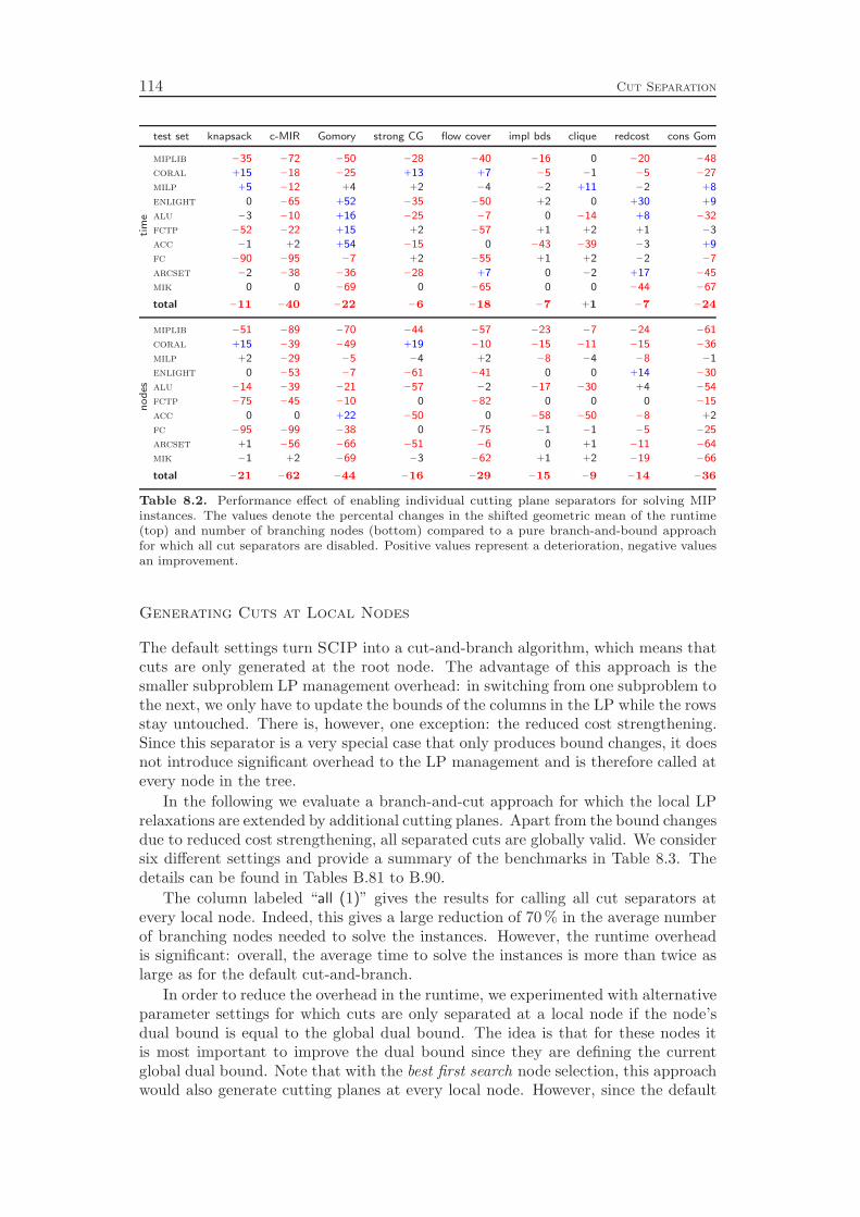
114 Cut Separation
test set knapsack c-MIR Gomory strong CG flow cover impl bds clique redcost cons Gomti
me
miplib −35 −72 −50 −28 −40 −16 0 −20 −48
coral +15 −18 −25 +13 +7 −5 −1 −5 −27
milp +5 −12 +4 +2 −4 −2 +11 −2 +8
enlight 0 −65 +52 −35 −50 +2 0 +30 +9
alu −3 −10 +16 −25 −7 0 −14 +8 −32
fctp −52 −22 +15 +2 −57 +1 +2 +1 −3
acc −1 +2 +54 −15 0 −43 −39 −3 +9
fc −90 −95 −7 +2 −55 +1 +2 −2 −7
arcset −2 −38 −36 −28 +7 0 −2 +17 −45
mik 0 0 −69 0 −65 0 0 −44 −67
total −11 −40 −22 −6 −18 −7 +1 −7 −24
no
des
miplib −51 −89 −70 −44 −57 −23 −7 −24 −61
coral +15 −39 −49 +19 −10 −15 −11 −15 −36
milp +2 −29 −5 −4 +2 −8 −4 −8 −1
enlight 0 −53 −7 −61 −41 0 0 +14 −30
alu −14 −39 −21 −57 −2 −17 −30 +4 −54
fctp −75 −45 −10 0 −82 0 0 0 −15
acc 0 0 +22 −50 0 −58 −50 −8 +2
fc −95 −99 −38 0 −75 −1 −1 −5 −25
arcset +1 −56 −66 −51 −6 0 +1 −11 −64
mik −1 +2 −69 −3 −62 +1 +2 −19 −66
total −21 −62 −44 −16 −29 −15 −9 −14 −36
Table 8.2. Performance effect of enabling individual cutting plane separators for solving MIPinstances. The values denote the percental changes in the shifted geometric mean of the runtime(top) and number of branching nodes (bottom) compared to a pure branch-and-bound approachfor which all cut separators are disabled. Positive values represent a deterioration, negative valuesan improvement.
Generating Cuts at Local Nodes
The default settings turn SCIP into a cut-and-branch algorithm, which means thatcuts are only generated at the root node. The advantage of this approach is thesmaller subproblem LP management overhead: in switching from one subproblem tothe next, we only have to update the bounds of the columns in the LP while the rowsstay untouched. There is, however, one exception: the reduced cost strengthening.Since this separator is a very special case that only produces bound changes, it doesnot introduce significant overhead to the LP management and is therefore called atevery node in the tree.
In the following we evaluate a branch-and-cut approach for which the local LPrelaxations are extended by additional cutting planes. Apart from the bound changesdue to reduced cost strengthening, all separated cuts are globally valid. We considersix different settings and provide a summary of the benchmarks in Table 8.3. Thedetails can be found in Tables B.81 to B.90.
The column labeled “all (1)” gives the results for calling all cut separators atevery local node. Indeed, this gives a large reduction of 70 % in the average numberof branching nodes needed to solve the instances. However, the runtime overheadis significant: overall, the average time to solve the instances is more than twice aslarge as for the default cut-and-branch.
In order to reduce the overhead in the runtime, we experimented with alternativeparameter settings for which cuts are only separated at a local node if the node’sdual bound is equal to the global dual bound. The idea is that for these nodes itis most important to improve the dual bound since they are defining the currentglobal dual bound. Note that with the best first search node selection, this approachwould also generate cutting planes at every local node. However, since the default
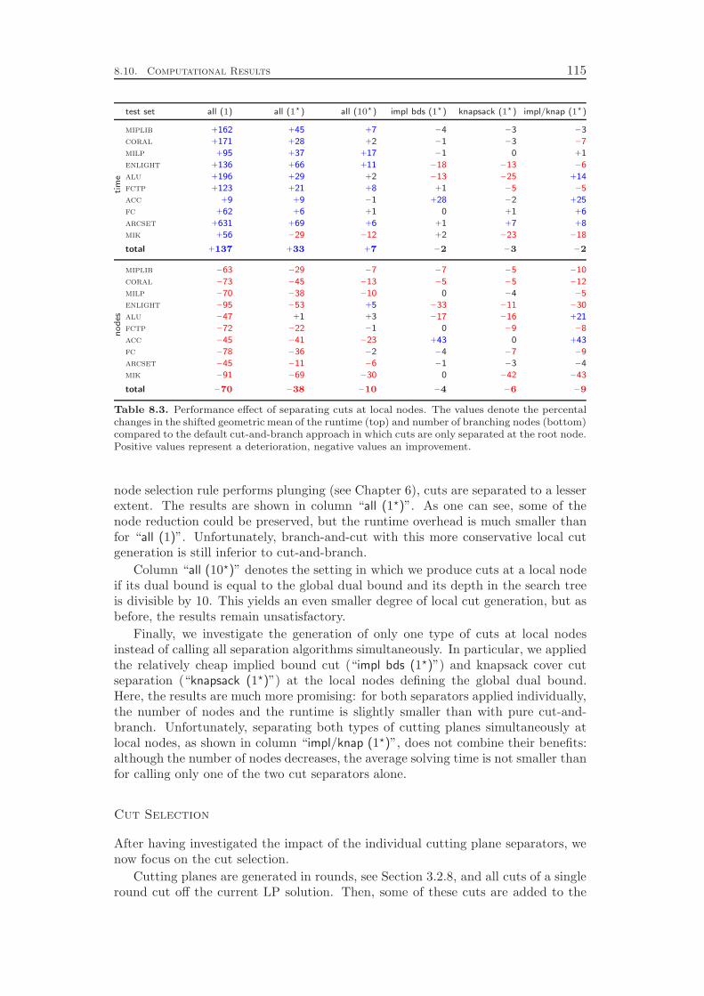
8.10. Computational Results 115
test set all (1) all (1⋆) all (10⋆) impl bds (1⋆) knapsack (1⋆) impl/knap (1⋆)ti
me
miplib +162 +45 +7 −4 −3 −3
coral +171 +28 +2 −1 −3 −7
milp +95 +37 +17 −1 0 +1
enlight +136 +66 +11 −18 −13 −6
alu +196 +29 +2 −13 −25 +14
fctp +123 +21 +8 +1 −5 −5
acc +9 +9 −1 +28 −2 +25
fc +62 +6 +1 0 +1 +6
arcset +631 +69 +6 +1 +7 +8
mik +56 −29 −12 +2 −23 −18
total +137 +33 +7 −2 −3 −2
no
des
miplib −63 −29 −7 −7 −5 −10
coral −73 −45 −13 −5 −5 −12
milp −70 −38 −10 0 −4 −5
enlight −95 −53 +5 −33 −11 −30
alu −47 +1 +3 −17 −16 +21
fctp −72 −22 −1 0 −9 −8
acc −45 −41 −23 +43 0 +43
fc −78 −36 −2 −4 −7 −9
arcset −45 −11 −6 −1 −3 −4
mik −91 −69 −30 0 −42 −43
total −70 −38 −10 −4 −6 −9
Table 8.3. Performance effect of separating cuts at local nodes. The values denote the percentalchanges in the shifted geometric mean of the runtime (top) and number of branching nodes (bottom)compared to the default cut-and-branch approach in which cuts are only separated at the root node.Positive values represent a deterioration, negative values an improvement.
node selection rule performs plunging (see Chapter 6), cuts are separated to a lesserextent. The results are shown in column “all (1⋆)”. As one can see, some of thenode reduction could be preserved, but the runtime overhead is much smaller thanfor “all (1)”. Unfortunately, branch-and-cut with this more conservative local cutgeneration is still inferior to cut-and-branch.
Column “all (10⋆)” denotes the setting in which we produce cuts at a local nodeif its dual bound is equal to the global dual bound and its depth in the search treeis divisible by 10. This yields an even smaller degree of local cut generation, but asbefore, the results remain unsatisfactory.
Finally, we investigate the generation of only one type of cuts at local nodesinstead of calling all separation algorithms simultaneously. In particular, we appliedthe relatively cheap implied bound cut (“impl bds (1⋆)”) and knapsack cover cutseparation (“knapsack (1⋆)”) at the local nodes defining the global dual bound.Here, the results are much more promising: for both separators applied individually,the number of nodes and the runtime is slightly smaller than with pure cut-and-branch. Unfortunately, separating both types of cutting planes simultaneously atlocal nodes, as shown in column “impl/knap (1⋆)”, does not combine their benefits:although the number of nodes decreases, the average solving time is not smaller thanfor calling only one of the two cut separators alone.
Cut Selection
After having investigated the impact of the individual cutting plane separators, wenow focus on the cut selection.
Cutting planes are generated in rounds, see Section 3.2.8, and all cuts of a singleround cut off the current LP solution. Then, some of these cuts are added to the

116 Cut Separation
test set one per round take all no obj paral no orthoti
me
miplib +97 +105 +4 +28
coral +98 +38 −8 +19
milp +27 +45 −7 +11
enlight +85 −17 −3 +8
alu −3 +1 +18 −16
fctp +7 +69 +6 +17
acc +1853 +351 −22 +313
fc +80 +694 +7 +102
arcset +35 +49 +6 +1
mik +247 +676 +7 +8
total +79 +71 −3 +22
no
des
miplib +3 −8 +2 −7
coral +3 −7 −9 −3
milp −4 −1 −8 −21
enlight +95 −29 −2 +10
alu −13 −24 +18 −25
fctp −10 −7 +10 +2
acc +258 +128 −32 +85
fc +140 −24 +6 +11
arcset +50 −42 +12 0
mik +312 +27 +4 −6
total +11 −5 −5 −8
Table 8.4. Performance effect of different cutting plane selection strategies for solving MIP in-stances. The values denote the percental changes in the shifted geometric mean of the runtime (top)and number of branching nodes (bottom) compared to the default procedure given in Section 3.3.8.Positive values represent a deterioration, negative values an improvement.
LP, and the modified LP is solved afterwards, followed by the next round of cuttingplane separation.
The task of the cutting plane selection is to decide which of the cuts of a singleseparation round should enter the LP and which should be discarded. Algorithm 3.2on page 49 shows the procedure that is employed by SCIP. The computationalresults for some variants of cutting plane selection can be found in the summaryTable 8.4 and in the detailed Tables B.91 to B.100.
The columns “one per round” and “take all” denote the trivial strategies of addingonly the most violated (in the Euclidean norm) or all of the generated cuts, respec-tively. As the results show, both rules are clearly inferior to the more involvedselection that is applied in the default settings. The columns “no obj paral” and“no ortho” evaluate the two supplementary criteria objective parallelism and orthog-onality of the cut selection Algorithm 3.2. In the former settings, we disabled theparallelism measurement by setting wp = 0. For the latter, we set wo = 0 andminortho = 0. One can see that the parallelism to the objective function does notplay a significant role; disabling this criterion even yields a slight performance im-provement. In contrast, the orthogonality within the set of selected cuts seems tobe crucial: selecting the cuts in this way improves the overall performance by 22 %.The largest impact can be seen on the acc and fc instances, for which the runtimesquadruple and double, respectively, if the orthogonality calculation is disabled.
Chapter 9
Primal Heuristics
The branch-and-bound algorithm to solve mixed integer programs is a so-calledcomplete procedure. This means, apart from numerical issues, it is guaranteed tofind the optimal solution for every problem instance in a finite amount of time.However, it is a very expensive method and has a worst case runtime which isexponential in the size of the problem instance.
In contrast, primal heuristics are incomplete methods. They try to find feasiblesolutions of good quality in a reasonably short period of time, but there is no guar-antee that they will succeed in finding a solution, least of all an optimal solution.Nevertheless, primal heuristics have a significant relevance as supplementary proce-dures inside a complete MIP solver: they help to find good feasible solutions earlyin the search process. An early discovering of a feasible solution has the followingadvantages:
⊲ It proves that the model is feasible, which is an indication that there is noerror in the model.
⊲ A user may already be satisfied with the quality of the heuristic solution, suchthat he can abort the solving process at an early stage.
⊲ Feasible solutions help to prune the search tree by bounding, thereby reducingthe work of the branch-and-bound algorithm.
⊲ The better the current incumbent is, the more reduced cost fixing and otherdual reductions can be applied to tighten the problem formulation, see Sec-tions 7.6 and 7.7.
There exists a large variety of mixed integer programming heuristics proposed inthe literature, including Hillier [116], Balas and Martin [33], Saltzman and Hillier [197],Glover and Laguna [95, 96, 97], Løkketangen and Glover [150], Glover et al. [98],Nediak and Eckstein [170], Balas et al. [32, 34], Fischetti and Lodi [85], Fischetti,Glover, and Lodi [84], Bertacco, Fischetti, and Lodi [40], Danna, Rothberg, andLe Pape [72], and Achterberg and Berthold [2]. Some of the heuristics available inSCIP are direct implementations of ideas found in the literature, some are variationsof the proposals, and some of them are newly developed techniques.
The primal heuristics of SCIP can be grouped into four categories:
⊲ Rounding heuristics try to round the fractional values of an LP solution suchthat the rounded integral vector stays feasible for the constraints.
⊲ Diving heuristics start from the current LP solution and iteratively fix aninteger variable to an integral value and resolve the LP.
⊲ Objective diving heuristics are similar to diving heuristics, but instead of fixingthe variables by modifying the bounds, they drive the variables into a desireddirection by modifying their objective coefficients.
117
118 Primal Heuristics
⊲ Improvement heuristics consider one or more primal feasible solutions thathave been previously found and try to construct an improved solution withbetter objective value.
We describe the individual heuristics contained in these classes only very brieflyin Sections 9.1 to 9.4 and present computational results in Section 9.5. Detaileddescriptions of the algorithms and an in-depth analysis of their computational impactcan by found in the diploma thesis of Timo Berthold [41].
RENS, Octane, and all of the improvement heuristics in Section 9.4 have beenimplemented by Timo Berthold. The implementation of the feasibility pump is jointwork with Timo Berthold. The remaining heuristics have been implemented by theauthor of this thesis.
9.1 Rounding Heuristics
Rounding heuristics start with a fractional vector x ∈ Rn that satisfies the linearconstraints ATx ≤ b and bounds l ≤ x ≤ u of the MIP but violates some of theintegrality restrictions. Usually, we take the optimal solution of the LP relaxationQLP of the current subproblem Q as starting point. Now, the task of a classicalrounding heuristic is to round the fractional values xj , j ∈ F := {j ∈ I | xj /∈ Z} ⊆ I,of the integer variables down or up such that the final integral vector x ∈ ZI × RC
still satisfies all linear constraints. More involved heuristics of this type also modifycontinuous variables or integer variables that already have integral values in orderto restore linear feasibility which has been lost due to the rounding of fractionalvariables.
9.1.1 RENS
Let x ∈ Rn be an optimal solution of the current subproblem’s LP relaxation, andlet F ⊆ I be the set of integer variables with fractional value. Then, there are2|F | possible roundings of x. The relaxation enforced neighborhood search (RENS)heuristic, which was invented by Berthold [41], constructs a sub-MIP
(MIP′) c⋆ = min {cTx | Ax ≤ b, x ∈ Rn, xj ∈ {⌊xj⌋, ⌈xj⌉} for all j ∈ I}
and solves it with SCIP in order to find the best possible feasible rounding if oneexists. Note that in this sub-MIP all integer variables with integral values are fixed,and the ones with fractional values are restricted to be rounded down or up. Thismeans, we can convert all integer variables into binary variables during presolving,see Section 10.5, to obtain a mixed binary program.
The issue with RENS is that the sub-MIP might still be very expensive to solve.Therefore, we only apply RENS at the root node of the search tree and abort thesub-MIP solving process after either a total of 5000 nodes has been processed or noimprovement of the sub-MIP incumbent has been found for 500 consecutive nodes.Additionally, we skip the heuristic if |F | > 1
2|I| since this suggests that the sub-
MIP is not sufficiently easier than the original MIP. Apart from the number ofintegral variables, which is an indicator for the “IP complexity” of the model, thetotal number of variables is also relevant for the solving speed of the sub-MIP sinceit gives a hint of the “LP complexity” of the instance. Therefore, we compare thetotal number of variables of the sub-MIP after presolving to the total number of
9.1. Rounding Heuristics 119
variables in the presolved version of the original instance. We only proceed withthe sub-MIP solving process if the number of variables has been reduced by at least25 %.
9.1.2 Simple Rounding
As the name suggests, simple rounding is a very simple and fast heuristic to rounda fractional solution to a feasible integral vector. The idea is based on the variablelock numbers, see Definition 3.3 on page 38. Consider a variable xj , j ∈ F ⊆ I, withfractional LP solution xj . If ζ−j = 0, we can safely set xj := ⌊xj⌋ without violating
any linear constraint. On the other hand, if ζ+j = 0, we can set xj := ⌈xj⌉. The
heuristic will succeed if all fractional variables j ∈ F have either ζ−j = 0 or ζ+j = 0.
Since the simple rounding heuristic is very fast, it is applied after the solvingof every LP. This includes the intermediate LPs in the cutting plane separationloop and the LPs that are solved by other heuristics such as the diving heuristics ofSection 9.2.
9.1.3 Rounding
The rounding heuristic is more involved than the simple rounding heuristic, but thesolutions found by rounding are a superset of the ones that can be found by simplerounding. The rounding is applied to all fractional variables j ∈ F , even if this leadsto an infeasibility in the linear constraints. After having generated an infeasibility ittries to select the rounding of the next variable such that the infeasibility is reducedor eliminated.
In a first step, the heuristic sets x := x and calculates the activities αi(x) =(ai)T x of the linear constraints. Then, it iterates over the set F of fractional vari-ables. If the current activity vector is feasible, i.e., β ≤ α(x) ≤ β, we select afractional variable with the largest number of variable locks max{ζ−j , ζ
+j } and round
it into the “more feasible” direction, i.e., downwards if ζ−j ≤ ζ+j and upwards other-
wise. The rationale behind this choice is to avoid the roundings that can break thefeasibility of many constraints.
If the current activity vector violates one or more constraints, we select one of theconstraints and try to find a fractional variable that can be rounded in a directionsuch that the violation of the constraint is decreased. If there is a choice, we selecta variable with a minimum number of variable locks in the corresponding directionin order to decrease the feasibility of as few other constraints as possible. If norounding can decrease the violation of the infeasible constraint, we abort.
In the default settings, rounding is also called after the solving of every LP inthe search tree, but not on the LPs that are solved inside other heuristics.
9.1.4 Shifting
The shifting heuristic is equal to the rounding heuristic, but it tries to continue in thecase that no rounding can decrease the violation of an infeasible constraint. In thiscase, we shift the value of a continuous variable or an integer variable with integralvalue in order to decrease the violation of the constraint. In the process, we haveto make sure to not run into a cycle. Therefore, we penalize the repeated shiftingin opposite directions of a variable, we randomize the selection of the infeasible row
120 Primal Heuristics
for which the violation should be reduced, and we abort after 50 successive shiftingshave been performed without decreasing the number of violated rows or the numberof fractional variables.
As shifting is already quite time consuming, we only call it in every 10’th depthlevel of the search tree.
9.1.5 Integer Shifting
Integer shifting is closely related to shifting, but it deals differently with continuousvariables. The first step is to relax all constraints in order to remove the continuousvariables. For each individual constraint aTx ≤ β the minimal contribution ajxj
of the continuous variables xj , j ∈ C, is moved to the right hand side. This isperformed by substituting the variable with its lower bound lj if aj ≥ 0 and withits upper bound uj if aj < 0.
Then, we apply the shifting heuristic in order to find an integer solution for therelaxed inequality system. If this was successful, we go back to the original MIP,fix all integer variables to their values in the solution for the relaxed system, andsolve the resulting LP to get optimal values for the continuous variables. If the LPis feasible, we have found a feasible solution for the original MIP.
9.1.6 Octane
Octane is a heuristic for pure binary programs which is due to Balas et al. [32]. Thename is an acronym for “octahedral neighborhood search”. The idea is to associateevery vertex of the hypercube [0, 1]n with the corresponding facet of the hypercube’sdual polytope, the n-dimensional octahedron. Then, starting from the point in theoctahedron that corresponds to the LP solution, rays are shot in various directions,and it is tested whether one of the facet defining hyperplanes that are hit by someray corresponds to a feasible point x ∈ {0, 1}n, Ax ≤ b. It can be exploited thatsuccessive facet hyperplanes hit by a ray correspond to 0/1 vectors that only differin one entry, which makes the updating procedure in the ray tracing algorithm veryefficient.
As Balas et al. proposed, we apply Octane only on the fractional subspace RF ,i.e., all variables xj , j ∈ I \ F , with integral value are fixed to their current val-ues. This approach significantly speeds up the computations without decreasing theheuristic’s ability to find good solutions too much. Applying Octane only on thefractional variables means to search for a rounded solution x of x. Therefore, thisversion of Octane is indeed a rounding heuristic in the classical sense.
9.2 Diving Heuristics
The general principle of diving heuristics is illustrated in Algorithm 9.1. Startingwith an optimal solution of the current subproblem’s LP relaxation, we round afractional variable, propagate the bound change, and resolve the LP. Since the LPbasis stays dual feasible after changing the bounds of the variables, the resolve can beefficiently conducted using the dual simplex algorithm. The rounding and resolvingprocedure is iterated until either the LP becomes infeasible or an integral solutionis found. One level of backtracking may optionally be applied in Step 8.
Of course, we use additional conditions to control the termination of the diving
9.2. Diving Heuristics 121
Algorithm 9.1 Generic Diving Heuristic
Input : Optimal LP solution x of current subproblem.
Output : If available, one or more feasible integral solutions.
1. Set x := x.
2. If F := {j ∈ I | xj /∈ Z} = ∅, stop and return the feasible integral solution x.
3. Apply the simple rounding heuristic of Section 9.1.2 on x to potentially producean intermediate feasible integral solution.
4. Choose a fractional variable xj , j ∈ F , and a rounding direction.
5. If down rounding is selected, tighten uj := ⌊xj⌋. Otherwise, tighten lj := ⌈xj⌉.
6. Call domain propagation to propagate the tightened bound.
7. Resolve the LP relaxation with the new bounds.
8. (optional) If the LP is infeasible, undo the previous propagations, apply theopposite rounding, propagate, and resolve the LP again.
9. If the LP is still infeasible, stop with a failure. Otherwise, let x be the newoptimal solution and goto Step 2.
loop in order to avoid too expensive dives. In SCIP, the main abort criterion isbased on the total number of simplex iterations used for the LP resolves in Steps 7and 8. For most heuristics we demand that this number must stay below 5 % of thecurrent total number of simplex iterations used for solving the regular LP relaxationsof the branch-and-bound nodes.
The only difference in the following implementations of the generic diving heuris-tic is how the selection in Step 4 is conducted. A common feature that is sharedby all diving heuristics is that variables xj are avoided in the selection that haveζ−j = 0 or ζ+
j = 0, since they can be rounded to integral values anyway by the simplerounding heuristic in Step 3. Additionally, we usually prefer binary variables overgeneral integer variables, since in most MIP models the binary variables representthe most crucial decisions.
9.2.1 Coefficient Diving
Coefficient Diving selects a variable xj in Step 4 of Algorithm 9.1 that minimizesmin{ζ−j , ζ
+j } but, as noted above, has min{ζ−j , ζ
+j } ≥ 1. The variable is rounded
in the direction of the smaller variable lock number. As a tie breaker, we chose avariable that has the smallest distance from its fractional value to the rounded value.
The rationale behind this selection is that this rounding reduces the feasibilityof only a small number of constraints and thereby hopefully leads to a small numberof violated constraints that have to be fixed by the LP resolve.
9.2.2 Fractionality Diving
In fractionality diving we select a variable with minimal fractionality φ(xj) = min{xj−⌊xj⌋, ⌈xj⌉ − xj}, which is rounded to the nearest integer. This selection rule seemsto be a very natural choice as it tries to produce a rounding that stays close to the
122 Primal Heuristics
LP solution.
9.2.3 Guided Diving
Guided diving was invented by Danna, Rothberg, and Le Pape [72]. As it needs afeasible integral solution as input, it can also be viewed as an improvement heuristic.However, it perfectly fits into the generic diving scheme of Algorithm 9.1 and istherefore presented here.
Danna et al. propose to use guided diving inside the branch-and-bound searchtree as a child selection rule during a plunge, compare Chapter 6: the variable tobranch on is selected by the regular branching rule, but the child to process next ischosen such that the value of the branching variable is driven into the direction ofthe variable’s value xj in the current incumbent solution. The hope is that thereare more feasible solutions in the vicinity of the current incumbent, and therefore,the search should be guided to that area.
In contrast, guided diving as implemented in SCIP works outside the tree justlike all other diving heuristics. Therefore, we have the additional choice of selectingthe variable to round. Similar to fractionality diving, we select the variable that isclosest to its value in the incumbent solution.
9.2.4 Line Search Diving
The line search diving heuristic converts the child selection idea of Martin [159], seeSection 6.1, into a diving heuristic: if a variable xj with value (xR)j in the root nodeof the search tree has now a value xj < (xR)j , the value of the variable seems to bepushed downwards on the path from the root node to the current node. Therefore,the idea is to further reinforce this pushing by rounding the variable down.
The geometric interpretation is as follows. We connect the root node LP solutionxR with the current solution x by a line and extend this line until we hit an integervalue for one of the fractional integer variables. The first variable for which thishappens is rounded into the corresponding direction. Algebraically spoken, we round
the variable which has the smallest distance ratioxj−⌊xj⌋(xR)j−xj
for xj < (xR)j and⌈xj⌉−xj
xj−(xR)jfor xj > (xR)j .
9.2.5 Pseudocost Diving
In Step 4 of Algorithm 9.1, pseudocost diving selects the variable with respect to thepseudocost values Ψ−j and Ψ+
j that have been collected during the search process.The pseudocosts give an estimate for each integer variable xj on how much the LPobjective value increases per unit change of the variable, see Section 5.3.
For each fractional variable xj , j ∈ F , we decide whether we want to round itdown or up. The primary criterion is similar as in the line search diving heuristic:if the difference of the current value xj to the root LP value (xR)j gives a strongindication that the variable is pushed to a certain direction, we select this directionfor the rounding. To be more specific, if xj < (xR)j − 0.4, we choose downwardsrounding, if xj > (xR)j + 0.4, we select upwards rounding. If the difference to theroot solution does not yield a decision, we look at the fractional part of the variable.If xj − ⌊xj⌋ < 0.3 we round down, if xj − ⌊xj⌋ > 0.7, we round up. If this still doesnot lead to a conclusion, we round down if Ψ−j < Ψ+
j and round up otherwise.
9.3. Objective Diving Heuristics 123
After having decided for each variable in which direction it should be rounded,we select a variable for the actual rounding that maximizes
√
⌈xj⌉ − xj ·1 + Ψ+
j
1 + Ψ−j(downwards) or
√
xj − ⌊xj⌋ ·1 + Ψ−j
1 + Ψ+j
(upwards),
respectively. This measure combines the fractionality of the variable with a pseudo-cost ratio. It prefers variables that are close to their rounded value and for whichthe estimated objective change per unit is much smaller in the selected directionthan in the opposite direction.
9.2.6 Vector Length Diving
The vector length diving heuristic is specifically tailored towards set covering and setpartitioning models, although it can also be applied to general MIPs. The idea is tochoose a rounding that covers the largest number of constraints with the smallestpossible objective value deterioration. The rounding direction for each variable isselected to be opposite to the objective function direction, i.e., we round up if cj ≥ 0and down otherwise. Since set covering or partitioning models usually have c ≥ 0we will always fix the binary variables in these models to 1.
In order to decide which fractional variable we want to round, we look at theratio
f−j cj
|A·j |+ 1(downwards) or
f+j cj
|A·j |+ 1(upwards)
of the direct objective increase and the number of constraints the variable is con-tained in. Since we always round up for set covering or partitioning models, theobjective increase would be f+
j cj , and the length of the sparse column vector |A·j |indicates how many constraints would be covered by the fixing of the variable to 1.Therefore, we select a variable with smallest ratio in order to minimize the costs percovered constraint.
9.3 Objective Diving Heuristics
In contrast to the “hard rounding” of diving heuristics that is conducted by tight-ening a bound of a variable, objective diving heuristics apply “soft rounding” byincreasing or decreasing the objective coefficient of the variable in order to push itinto the desired direction without actually forcing it to the rounded value. Such asoft rounding does not entail the risk of obtaining an infeasible LP. The downsideis that we can no longer apply domain propagation, and that the size of the LP isnot implicitly reduced as it is in regular diving due to the fixings of variables totheir lower or upper bounds. Furthermore, we have to deactivate the objective limitimposed by the current incumbent, because the objective function does no longercoincide with the objective of the MIP. Additionally, we have to find means to avoidcycling.
The general approach to objective diving is similar to Algorithm 9.1 for regulardiving. In Step 5, the tightening of the local bounds is replaced by a correspondingchange in the objective function, the domain propagation of Step 6 and the back-tracking of Step 8 are skipped, and the infeasibility of the LP is no longer an abort
124 Primal Heuristics
criterion. Note that the LPs can be resolved efficiently with the primal simplex al-gorithm, since a change in the objective function does not destroy primal feasibilityof a previously optimal simplex basis.
9.3.1 Objective Pseudocost Diving
Objective pseudocost diving shares the ideas of pseudocost diving but primarilyuses soft rounding via the objective function instead of hard rounding with boundchanges. The variable and direction are selected according to the same criterionas in pseudocost diving. If the variable xj should be rounded down, we change itsobjective coefficient to cj := 1000(d+1) · |cj| with d being the current diving depth,i.e., the number of LP resolves that have been performed during the dive. If thevariable should be rounded up, we use the negative of this value.
For each variable, we remember whether it was already soft-rounded downwardsor upwards. If a variable should be rounded a second time, we apply a hard roundinginto the other direction by changing its lower or upper bound. The rationale behindthis approach is the following: if a variable could not be driven, for example, to itslower bound by dramatically increasing its objective coefficient, we take this as anindication that fixing it to its lower bound would probably generate an infeasibleLP. Therefore, we apply a hard rounding into the opposite direction and round thevariable upwards.
After imposing a bound change, we resolve the LP with the dual simplex algo-rithm. In this case, it may happen that the modified LP turns out to be infeasible,which leads to the termination of the heuristic.
9.3.2 Root Solution Diving
The root solution diving is the objective diving analogon to the line search divingheuristic. As in objective pseudocost diving we augment the soft roundings with hardroundings in order to avoid cycling. However, the approach to combine the objectiveand bound changes is slightly different.
In each iteration, we scale the current objective function with a factor of 0.9,thereby slowly fading out the original objective coefficients. A soft rounding isapplied by increasing or decreasing the objective coefficient of the rounding variableby 0.1 · max{|c|, 1}, with c being the objective value of the LP solution at thesubproblem where the dive was started. We count the number of downwards andupwards soft roundings for each variable, and if the difference of these countersbecomes larger or equal to 10, we permanently apply a hard rounding into thepreferred direction by modifying the lower or upper bound of the variable. If atany time a variable that has already been soft-rounded becomes integral, we fix thevariable to this value by changing both of its bounds.
9.3.3 Feasibility Pump
The feasibility pump is a sophisticated objective diving heuristic that was inventedby Fischetti, Glover, and Lodi [84] for pure integer programs and generalized byBertacco, Fischetti, and Lodi [40] to mixed integer programs. Achterberg andBerthold [2] proposed a slight modification of the heuristic which they call objectivefeasibility pump and that yields feasible solutions of better objective value.
Starting as usual from the optimal solution x of the current subproblem’s LP
9.4. Improvement Heuristics 125
relaxation, the solution is rounded to a vector x = [x], with [ · ] defined by
[x]j :=
{⌊xj + 0.5⌋ if j ∈ Ixj if j ∈ C = N \ I.
(9.1)
If x is not feasible, an additional LP is solved in order to find a new point in the LPpolyhedron
P := {x ∈ Rn | Ax ≤ b, l ≤ x ≤ u}
which is, w.r.t. the integer variables I, closest to x, i.e., that minimizes
∆(x, x) :=∑
j∈I
|xj − xj |.
The procedure is iterated by using this point as new solution x ∈ P . Thereby,the algorithm creates two sequences of points: one with points x that fulfill theinequalities, and one with points x that fulfill the integrality requirements. Thealgorithm terminates if the two sequences converge or if a predefined iteration limitis reached.
In order to determine a point
x := argmin{∆(x, x) | x ∈ P} (9.2)
in P , which is nearest to x, the following LP is solved:
min∑
j∈I:xj=lj
(xj − lj) +∑
j∈I:xj=uj
(uj − xj) +∑
j∈I:lj<xj<uj
dj
s.t. Ax ≤ b
d ≥ x− x
d ≥ x− x
l ≤ x ≤ u.
(9.3)
The auxiliary variables dj are introduced to model the nonlinear function dj =|xj − xj | for integer variables xj , j ∈ I, that are not equal to one of their bounds inthe rounded solution x.
The implementation of the feasibility pump in SCIP is slightly different from theone proposed by Bertacco, Fischetti, and Lodi [40]. First, it involves the modifica-tions proposed in [2] to better guide the search into the area of solutions with goodobjective value. Second, it does not add auxiliary variables dj as in System (9.3)for general integer variables, because adding and deleting columns produces over-head for the LP solving. Instead, we set the objective coefficient to +1, −1, or 0,depending on whether we want to round the variable down or up, or leave it on itsintegral value. Of course, such an objective modification may lead to overshootingthe rounded value, and an objective of 0 does not necessarily mean that the vari-able will stay at its current value. As a third modification, we skip the expensiveenumeration phase which is performed in stage 3 of the original feasibility pumpalgorithm.
9.4 Improvement Heuristics
Starting from one or more feasible solutions, the goal of improvement heuristics is tofind feasible solutions with a better objective value. Besides the one opt heuristic,all improvement heuristics implemented in SCIP are solving a sub-MIP.

126 Primal Heuristics
The first to use sub-MIP solves inside a MIP heuristic have been Fischetti andLodi [85] with their local branching, although they did not think of it as a heuris-tic but as a different way of branching which is influenced by the current incum-bent. Danna, Rothberg, and Le Pape [72] adopted the idea of solving sub-MIPs forheuristic purposes and invented the relaxation induced neighborhood search (RINS)method, which they integrated into Cplex. Rothberg [194] continued to pursue thisapproach and developed mutation and crossover, which form the basis of Cplex’very successful “solution polishing”. Crossover was independently developed byTimo Berthold who implemented this heuristic in SCIP.
From the improvement heuristics, only one opt and crossover are active by de-fault. Berthold [41] observed that local branching deteriorates, but any of RINS,crossover, and mutation improves the performance of SCIP. However, combina-tions of these heuristics produce worse results on his test set. In total, crossoverturned out to be the most effective of the four individual sub-MIP improvementheuristics.
9.4.1 One Opt
The idea of one opt is very simple: given a feasible solution x, the value of a variablexj can be decreased for cj > 0 or increased for cj < 0 if the resulting solution x isstill feasible, i.e., Ax ≤ b and l ≤ x ≤ u. The modified solution would then have animproved objective value.
The version of one opt as implemented in SCIP first calculates a value δj ∈Z≥0 for each variable xj with j ∈ I and cj 6= 0. This value denotes how far thevariable can be shifted into the desired direction. If more than one variable can beshifted, they are sorted by non-decreasing objective improvement capability |cjδj |and consecutively shifted until no more improvements can be obtained. Finally, theinteger variables are fixed to their resulting values, and an LP is solved to obtainbest possible values for the continuous variables.
9.4.2 Local Branching
Local branching was proposed by Fischetti and Lodi [85]. It is based on the observa-tion that often primal feasible solutions have additional solutions in their vicin-ity. Therefore, Fischetti and Lodi implemented a branching scheme on top ofa MIP solver that would produce the case distinction
∑
j∈I |xj − xj | ≤ k and∑
j∈I |xj − xj | ≥ k + 1, k ∈ Z>0, with the former case being enumerated first.By dropping the requirement that the branch
∑
j∈I |xj − xj | ≤ k has to beenumerated exhaustively, the local branching scheme can be easily converted intoa primal improvement heuristic. However, some control of the neighborhood sizek is necessary. The SCIP implementation of local branching starts with k = 18.This value is increased by 50 % if a sub-MIP has been enumerated completely anddoes not contain a better solution than the current incumbent. The neighborhoodis decreased by 50 % if the sub-MIP solve was aborted due to the node limit thatwas applied.
9.4.3 RINS
The relaxation induced neighborhood search (RINS) solves sub-MIPs that are de-fined by the current incumbent solution x and the LP optimum x of the current
9.5. Computational Results 127
subproblem. RINS was invented by Danna, Rothberg, and Le Pape [72].The sub-MIP that is solved in RINS is defined as
min{cTx | Ax ≤ b, l ≤ x ≤ u, xj ∈ Z for all j ∈ I,
xj = xj for all j ∈ I with xj = xj},
which means that an integer variable is fixed if both the incumbent and the currentLP solution agree on a common value. As in the local branching heuristic, thedifficult part is to control the calling frequency and the sub-MIP node limit thatis applied to avoid spending too much time on the heuristic. Similar to the divingheuristics, the general approach in SCIP is to avoid spending more than a certainfraction (10 % in the case of RINS) of the total number of branching nodes for solvingthe sub-MIPs.
9.4.4 Mutation
Mutation and crossover are the two building blocks of a genetic algorithm. Roth-berg [194] applied this idea to mixed integer programming to develop an improve-ment heuristic, which he calls solution polishing. The mutation part as proposedby Rothberg is to start from a feasible solution and fix a certain fraction of thegeneral integer variables to their values. The actual variables to fix are selected ran-domly. Then, a sub-MIP is solved to identify the optimal values for the remainingvariables. Rothberg proposes to adjust the fixing rate dynamically. However, thecurrent implementation in SCIP chooses a static fixing rate of 80 %.
9.4.5 Crossover
A crossover of two or more feasible solutions is performed by fixing all integer vari-ables on which the solutions agree to their specific values and leaving the othervariables free in their global bounds. Thus, the more solutions participate in thecrossover, the fewer variables become fixed and the larger is the subspace that willbe enumerated in the sub-MIP. Like mutation, crossover was developed by Roth-berg [194]. Independently, it was invented by Berthold [41] and implemented inSCIP.
The crossover implementation of SCIP uses three solutions to define the sub-MIPs. By default, SCIP keeps the best 100 feasible solutions in a solution poolsorted by non-decreasing objective value. After a solution has been found that takesone of the first three slots in the pool, the crossover is performed on the best threesolutions. In the subsequent calls, a random selection of three solutions is used whichis biased towards the solutions of better objective value.
9.5 Computational Results
The following computational results assess the impact of the various primal heuristicspresented in the previous sections. We discuss the benchmarks only briefly, since avery detailed computational study of the MIP heuristics of SCIP can be found inBerthold [41].
In the default parameter settings, all primal heuristics except Octane, localbranching, RINS, and mutation are enabled. Table 9.1 yields the results for disabling
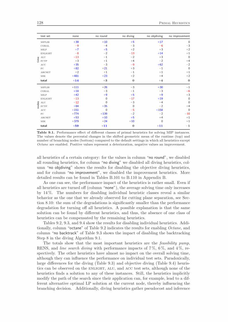
128 Primal Heuristics
test set none no round no diving no objdiving no improvementti
me
miplib +39 +10 +5 +17 0
coral −9 −4 −3 −6 −3
milp +7 +5 +2 +3 +2
enlight −8 −2 −13 +14 +1
alu −13 −1 −2 +3 0
fctp +3 +1 +4 −2 +4
acc +35 −3 −9 +62 −2
fc +82 +21 +3 −1 0
arcset +2 +1 −1 +1 +1
mik +481 +23 +2 +4 +2
total +14 +3 0 +4 0
no
des
miplib +111 +26 −3 +30 −1
coral +18 −3 −1 −3 −6
milp +42 +9 +5 +9 +3
enlight −13 0 −17 +19 0
alu −12 0 −3 −4 0
fctp +84 +35 0 −2 +4
acc +151 0 −5 +158 0
fc +774 +139 −2 −2 −10
arcset +53 +10 +5 +4 +1
mik +379 +24 +10 0 +1
total +59 +11 0 +11 −1
Table 9.1. Performance effect of different classes of primal heuristics for solving MIP instances.The values denote the percental changes in the shifted geometric mean of the runtime (top) andnumber of branching nodes (bottom) compared to the default settings in which all heuristics exceptOctane are enabled. Positive values represent a deterioration, negative values an improvement.
all heuristics of a certain category: for the values in column “no round”, we disabledall rounding heuristics, for column “no diving” we disabled all diving heuristics, col-umn “no objdiving” shows the results for disabling the objective diving heuristics,and for column “no improvement”, we disabled the improvement heuristics. Moredetailed results can be found in Tables B.101 to B.110 in Appendix B.
As one can see, the performance impact of the heuristics is rather small. Even ifall heuristics are turned off (column “none”), the average solving time only increasesby 14 %. The numbers for disabling individual heuristic classes reveal a similarbehavior as the one that we already observed for cutting plane separation, see Sec-tion 8.10: the sum of the degradations is significantly smaller than the performancedegradation for turning off all heuristics. A possible explanation is that the samesolution can be found by different heuristics, and thus, the absence of one class ofheuristics can be compensated by the remaining heuristics.
Tables 9.2, 9.3, and 9.4 show the results for disabling individual heuristics. Addi-tionally, column “octane” of Table 9.2 indicates the results for enabling Octane, andcolumn “no backtrack” of Table 9.3 shows the impact of disabling the backtrackingStep 8 in the diving Algorithm 9.1.
The totals show that the most important heuristics are the feasibility pump,RENS, and line search diving with performance impacts of 7 %, 6 %, and 4 %, re-spectively. The other heuristics have almost no impact on the overall solving time,although they can influence the performance on individual test sets. Paradoxically,large differences for the diving (Table 9.3) and objective diving (Table 9.4) heuris-tics can be observed on the enlight, alu, and acc test sets, although none of theheuristics finds a solution to any of these instances. Still, the heuristics implicitlymodify the path of the search since their application can, for example, lead to a dif-ferent alternative optimal LP solution at the current node, thereby influencing thebranching decision. Additionally, diving heuristics gather pseudocost and inference
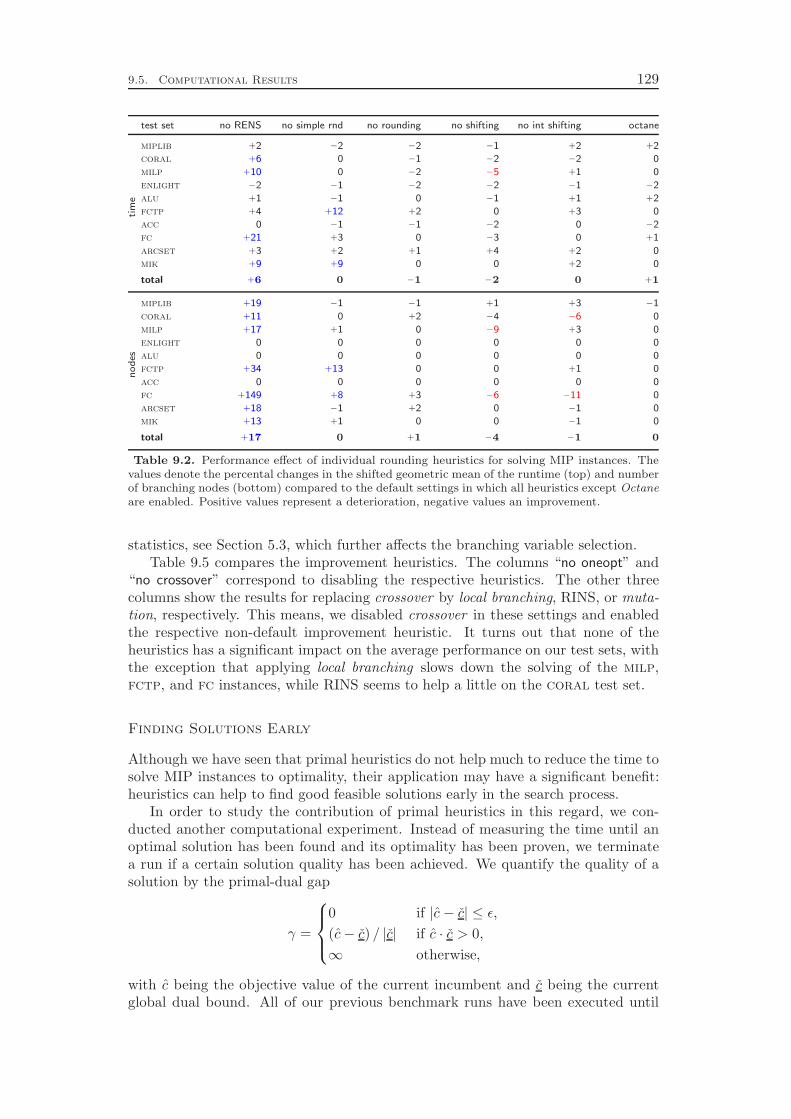
9.5. Computational Results 129
test set no RENS no simple rnd no rounding no shifting no int shifting octaneti
me
miplib +2 −2 −2 −1 +2 +2
coral +6 0 −1 −2 −2 0
milp +10 0 −2 −5 +1 0
enlight −2 −1 −2 −2 −1 −2
alu +1 −1 0 −1 +1 +2
fctp +4 +12 +2 0 +3 0
acc 0 −1 −1 −2 0 −2
fc +21 +3 0 −3 0 +1
arcset +3 +2 +1 +4 +2 0
mik +9 +9 0 0 +2 0
total +6 0 −1 −2 0 +1
no
des
miplib +19 −1 −1 +1 +3 −1
coral +11 0 +2 −4 −6 0
milp +17 +1 0 −9 +3 0
enlight 0 0 0 0 0 0
alu 0 0 0 0 0 0
fctp +34 +13 0 0 +1 0
acc 0 0 0 0 0 0
fc +149 +8 +3 −6 −11 0
arcset +18 −1 +2 0 −1 0
mik +13 +1 0 0 −1 0
total +17 0 +1 −4 −1 0
Table 9.2. Performance effect of individual rounding heuristics for solving MIP instances. Thevalues denote the percental changes in the shifted geometric mean of the runtime (top) and numberof branching nodes (bottom) compared to the default settings in which all heuristics except Octaneare enabled. Positive values represent a deterioration, negative values an improvement.
statistics, see Section 5.3, which further affects the branching variable selection.Table 9.5 compares the improvement heuristics. The columns “no oneopt” and
“no crossover” correspond to disabling the respective heuristics. The other threecolumns show the results for replacing crossover by local branching, RINS, or muta-tion, respectively. This means, we disabled crossover in these settings and enabledthe respective non-default improvement heuristic. It turns out that none of theheuristics has a significant impact on the average performance on our test sets, withthe exception that applying local branching slows down the solving of the milp,fctp, and fc instances, while RINS seems to help a little on the coral test set.
Finding Solutions Early
Although we have seen that primal heuristics do not help much to reduce the time tosolve MIP instances to optimality, their application may have a significant benefit:heuristics can help to find good feasible solutions early in the search process.
In order to study the contribution of primal heuristics in this regard, we con-ducted another computational experiment. Instead of measuring the time until anoptimal solution has been found and its optimality has been proven, we terminatea run if a certain solution quality has been achieved. We quantify the quality of asolution by the primal-dual gap
γ =
0 if |c − c| ≤ ǫ,
(c− c) / |c| if c · c > 0,
∞ otherwise,
with c being the objective value of the current incumbent and c being the currentglobal dual bound. All of our previous benchmark runs have been executed until
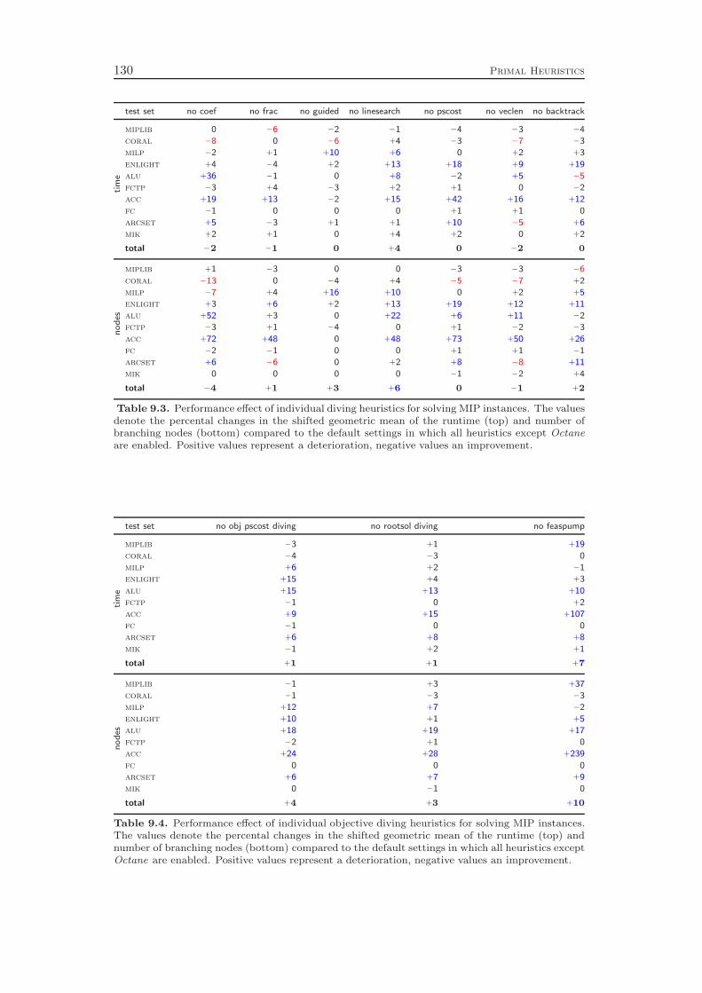
130 Primal Heuristics
test set no coef no frac no guided no linesearch no pscost no veclen no backtrackti
me
miplib 0 −6 −2 −1 −4 −3 −4
coral −8 0 −6 +4 −3 −7 −3
milp −2 +1 +10 +6 0 +2 +3
enlight +4 −4 +2 +13 +18 +9 +19
alu +36 −1 0 +8 −2 +5 −5
fctp −3 +4 −3 +2 +1 0 −2
acc +19 +13 −2 +15 +42 +16 +12
fc −1 0 0 0 +1 +1 0
arcset +5 −3 +1 +1 +10 −5 +6
mik +2 +1 0 +4 +2 0 +2
total −2 −1 0 +4 0 −2 0
no
des
miplib +1 −3 0 0 −3 −3 −6
coral −13 0 −4 +4 −5 −7 +2
milp −7 +4 +16 +10 0 +2 +5
enlight +3 +6 +2 +13 +19 +12 +11
alu +52 +3 0 +22 +6 +11 −2
fctp −3 +1 −4 0 +1 −2 −3
acc +72 +48 0 +48 +73 +50 +26
fc −2 −1 0 0 +1 +1 −1
arcset +6 −6 0 +2 +8 −8 +11
mik 0 0 0 0 −1 −2 +4
total −4 +1 +3 +6 0 −1 +2
Table 9.3. Performance effect of individual diving heuristics for solving MIP instances. The valuesdenote the percental changes in the shifted geometric mean of the runtime (top) and number ofbranching nodes (bottom) compared to the default settings in which all heuristics except Octaneare enabled. Positive values represent a deterioration, negative values an improvement.
test set no obj pscost diving no rootsol diving no feaspump
tim
e
miplib −3 +1 +19
coral −4 −3 0
milp +6 +2 −1
enlight +15 +4 +3
alu +15 +13 +10
fctp −1 0 +2
acc +9 +15 +107
fc −1 0 0
arcset +6 +8 +8
mik −1 +2 +1
total +1 +1 +7
no
des
miplib −1 +3 +37
coral −1 −3 −3
milp +12 +7 −2
enlight +10 +1 +5
alu +18 +19 +17
fctp −2 +1 0
acc +24 +28 +239
fc 0 0 0
arcset +6 +7 +9
mik 0 −1 0
total +4 +3 +10
Table 9.4. Performance effect of individual objective diving heuristics for solving MIP instances.The values denote the percental changes in the shifted geometric mean of the runtime (top) andnumber of branching nodes (bottom) compared to the default settings in which all heuristics exceptOctane are enabled. Positive values represent a deterioration, negative values an improvement.
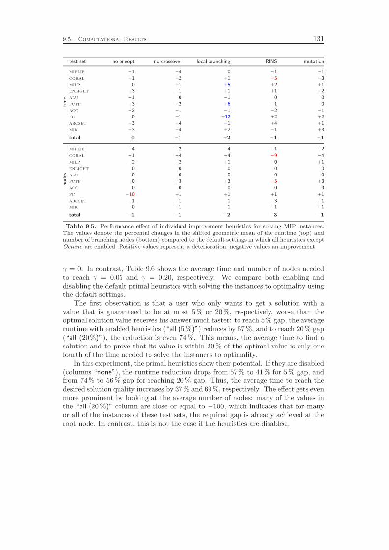
9.5. Computational Results 131
test set no oneopt no crossover local branching RINS mutationti
me
miplib −1 −4 0 −1 −1
coral +1 −2 +1 −5 −3
milp 0 +1 +5 +2 +1
enlight −3 −1 +1 +1 −2
alu −1 0 −1 0 0
fctp +3 +2 +6 −1 0
acc −2 −1 −1 −2 −1
fc 0 +1 +12 +2 +2
arcset +3 −4 −1 +4 +1
mik +3 −4 +2 −1 +3
total 0 −1 +2 −1 −1
no
des
miplib −4 −2 −4 −1 −2
coral −1 −4 −4 −9 −4
milp +2 +2 +1 0 +1
enlight 0 0 0 0 0
alu 0 0 0 0 0
fctp 0 +3 +3 −5 +3
acc 0 0 0 0 0
fc −10 +1 +1 +1 +1
arcset −1 −1 −1 −3 −1
mik 0 −1 −1 −1 −1
total −1 −1 −2 −3 −1
Table 9.5. Performance effect of individual improvement heuristics for solving MIP instances.The values denote the percental changes in the shifted geometric mean of the runtime (top) andnumber of branching nodes (bottom) compared to the default settings in which all heuristics exceptOctane are enabled. Positive values represent a deterioration, negative values an improvement.
γ = 0. In contrast, Table 9.6 shows the average time and number of nodes neededto reach γ = 0.05 and γ = 0.20, respectively. We compare both enabling anddisabling the default primal heuristics with solving the instances to optimality usingthe default settings.
The first observation is that a user who only wants to get a solution with avalue that is guaranteed to be at most 5 % or 20 %, respectively, worse than theoptimal solution value receives his answer much faster: to reach 5 % gap, the averageruntime with enabled heuristics (“all (5 %)”) reduces by 57 %, and to reach 20 % gap(“all (20 %)”), the reduction is even 74 %. This means, the average time to find asolution and to prove that its value is within 20 % of the optimal value is only onefourth of the time needed to solve the instances to optimality.
In this experiment, the primal heuristics show their potential. If they are disabled(columns “none”), the runtime reduction drops from 57 % to 41 % for 5 % gap, andfrom 74 % to 56 % gap for reaching 20 % gap. Thus, the average time to reach thedesired solution quality increases by 37 % and 69 %, respectively. The effect gets evenmore prominent by looking at the average number of nodes: many of the values inthe “all (20 %)” column are close or equal to −100, which indicates that for manyor all of the instances of these test sets, the required gap is already achieved at theroot node. In contrast, this is not the case if the heuristics are disabled.
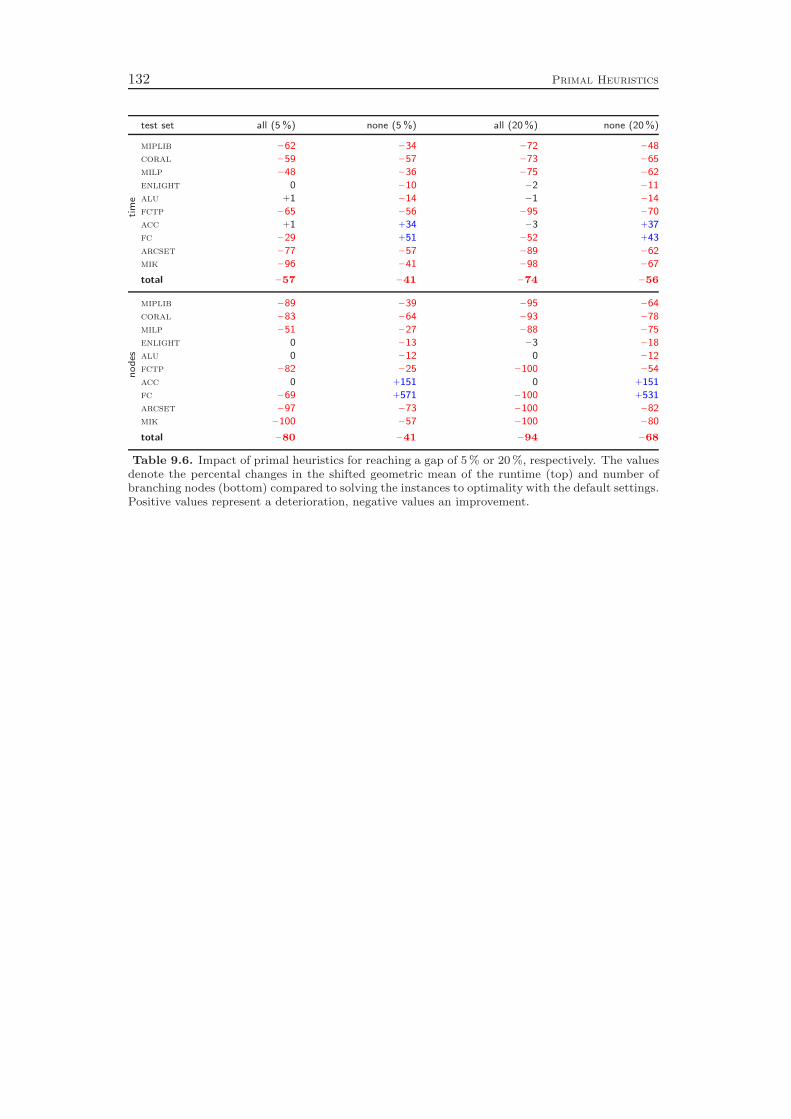
132 Primal Heuristics
test set all (5 %) none (5 %) all (20 %) none (20 %)ti
me
miplib −62 −34 −72 −48
coral −59 −57 −73 −65
milp −48 −36 −75 −62
enlight 0 −10 −2 −11
alu +1 −14 −1 −14
fctp −65 −56 −95 −70
acc +1 +34 −3 +37
fc −29 +51 −52 +43
arcset −77 −57 −89 −62
mik −96 −41 −98 −67
total −57 −41 −74 −56
no
des
miplib −89 −39 −95 −64
coral −83 −64 −93 −78
milp −51 −27 −88 −75
enlight 0 −13 −3 −18
alu 0 −12 0 −12
fctp −82 −25 −100 −54
acc 0 +151 0 +151
fc −69 +571 −100 +531
arcset −97 −73 −100 −82
mik −100 −57 −100 −80
total −80 −41 −94 −68
Table 9.6. Impact of primal heuristics for reaching a gap of 5 % or 20 %, respectively. The valuesdenote the percental changes in the shifted geometric mean of the runtime (top) and number ofbranching nodes (bottom) compared to solving the instances to optimality with the default settings.Positive values represent a deterioration, negative values an improvement.
Chapter 10
Presolving
Presolving is a way to transform the given problem instance into an equivalent in-stance that is (hopefully) easier to solve. Since many MIP instances appearing inpractice1 contain lots of irrelevant data that only slow down the solving process,all existing competitive MIP solvers feature some form of presolving. The mostfundamental presolving concepts for mixed integer programming are described inSavelsbergh [199]. Additional information can be found in Fügenschuh and Mar-tin [90].
The task of presolving is threefold: first, it reduces the size of the model byremoving irrelevant information such as redundant constraints or fixed variables.Second, it strengthens the LP relaxation of the model by exploiting integrality in-formation, e.g., to tighten the bounds of the variables or to improve coefficients inthe constraints. Third, it extracts information such as implications or cliquesfrom the model which can later be used, for example for branching or cutting planeseparation.
Applying the domain propagation of Chapter 7 to the global problem instance Ralready yields a simple form of presolving, namely the tightening of the variables’global bounds l ≤ x ≤ u. In addition to this, presolving employs more sophisticatedrules, which may alter the structure of the problem.
We distinguish between primal and dual presolving reductions. Primal reduc-tions are solely based on feasibility reasoning, while dual reductions consider theobjective function. The latter may exclude feasible solutions from the problem in-stance, as long as at least one optimal solution remains.
Sections 10.1 to 10.4 describe the presolving algorithms that are specialized to acertain type of constraints. These are implemented in the constraint handlers. Af-terwards in Sections 10.5 to 10.8, we deal with general purpose presolving algorithmsthat can be applied to any constraint integer program independently from the typeof the involved constraints. Section 10.9 presents restarts, a technique applied inSAT solvers that is new for the MIP community. The computational experimentsof Section 10.10 evaluate the impact of presolving on the overall solving process.
10.1 Linear Constraints
Recall that linear constraints in SCIP are defined as
β ≤ aTx ≤ β
with the left and right hand sides β, β ∈ R ∪ {±∞} and coefficients a ∈ Rn.The presolving of linear constraints is depicted in Algorithm 10.1. It commences
in Step 1 by looking at the individual constraints one at a time. For each constraint,
1in particular those that have been automatically generated, for example using a modelinglanguage such as Ampl [89] or Zimpl [133, 134]
133

134 Presolving
Algorithm 10.1 Presolving for Linear Constraints
1. For all linear constraints β ≤ aTx ≤ β:
(a) Normalize the constraint using Algorithm 10.2.
(b) If aj ∈ Z for all j ∈ N and aj = 0 for all j ∈ C, set β := ⌈β⌉ and β := ⌊β⌋.
(c) Tighten the bounds of the variables by calling domain propagation Algo-rithm 7.1.
(d) If α > β or α < β, the problem instance is infeasible.If α ≥ β, set β := −∞.If α ≤ β, set β := +∞.If β = −∞ and β = +∞, delete the constraint.
(e) If the constraint is a set partitioning constraint∑
j∈S xj = 1 or a setpacking constraint
∑
j∈S xj ≤ 1, xj ∈ {0, 1} for all j ∈ S, add clique Sto the clique table.
(f) For all j ∈ I with aj > 0, α+ aj ≥ β, and α− aj ≤ β:
i. Set a′j := max{β − α,α − β}.
ii. Set β := β − (aj − a′j)lj and β := β − (aj − a
′j)uj .
iii. Set aj := a′j .
For all j ∈ I with aj < 0, α− aj ≥ β, and α+ aj ≤ β:
i. Set a′j := min{α− β, β − α}.
ii. Set β := β − (aj − a′j)uj and β := β − (aj − a
′j)lj .
iii. Set aj := a′j .
(g) If the constraint or the bounds of the variables have been modified inSteps 1a to 1f, and if this loop has not already been executed 10 times,goto Step 1a.
(h) If the constraint is an equation, i.e., β = β, call Algorithm 10.3.
(i) Call the dual aggregation Algorithm 10.4.
2. If no reductions have been found yet in the current presolving round, call theconstraint pair presolving Algorithm 10.5.
3. If no reductions have been found yet in the current presolving round, call thedual bound reduction Algorithm 10.6.
4. If no reductions have been found yet in the current presolving round, callAlgorithm 10.7 for each linear constraint to upgrade it into a constraint of amore specific constraint type.
the first operation is the constraint normalization of Step 1a as illustrated in Algo-rithm 10.2. In the normalization, we remove fixed variables by subtracting theircontribution to the activity aTx of the constraint from the left and right hand sides.Aggregated and multi-aggregated variables xk
⋆=∑
j∈N sjxj + d are substituted fortheir defining affine linear expression, again subtracting the constant akd from theleft and right hand sides. Afterwards, we multiply the constraint by +1 or −1 inorder to reach a standard form, which simplifies the upgrading of the constraint intoa more specialized constraint type, see below.
In the next step of the normalization, we try to scale the constraint to obtainintegral coefficients. Since we are dealing with floating point arithmetic, this scaling
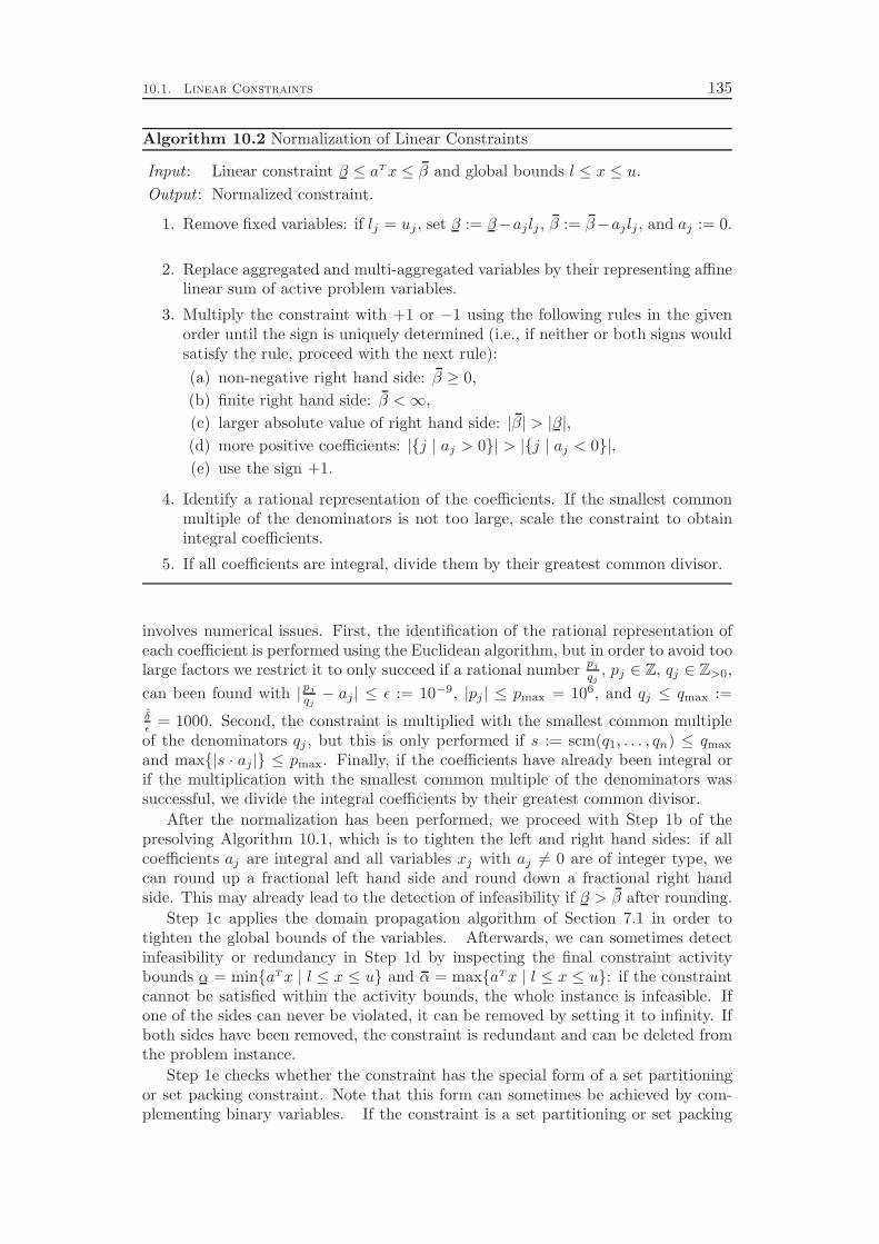
10.1. Linear Constraints 135
Algorithm 10.2 Normalization of Linear Constraints
Input : Linear constraint β ≤ aTx ≤ β and global bounds l ≤ x ≤ u.
Output : Normalized constraint.
1. Remove fixed variables: if lj = uj , set β := β−ajlj , β := β−ajlj , and aj := 0.
2. Replace aggregated and multi-aggregated variables by their representing affinelinear sum of active problem variables.
3. Multiply the constraint with +1 or −1 using the following rules in the givenorder until the sign is uniquely determined (i.e., if neither or both signs wouldsatisfy the rule, proceed with the next rule):
(a) non-negative right hand side: β ≥ 0,
(b) finite right hand side: β <∞,
(c) larger absolute value of right hand side: |β| > |β|,
(d) more positive coefficients: |{j | aj > 0}| > |{j | aj < 0}|,
(e) use the sign +1.
4. Identify a rational representation of the coefficients. If the smallest commonmultiple of the denominators is not too large, scale the constraint to obtainintegral coefficients.
5. If all coefficients are integral, divide them by their greatest common divisor.
involves numerical issues. First, the identification of the rational representation ofeach coefficient is performed using the Euclidean algorithm, but in order to avoid toolarge factors we restrict it to only succeed if a rational number
pj
qj, pj ∈ Z, qj ∈ Z>0,
can been found with |pj
qj− aj | ≤ ǫ := 10−9, |pj | ≤ pmax = 106, and qj ≤ qmax :=
δǫ
= 1000. Second, the constraint is multiplied with the smallest common multipleof the denominators qj , but this is only performed if s := scm(q1, . . . , qn) ≤ qmax
and max{|s · aj |} ≤ pmax. Finally, if the coefficients have already been integral orif the multiplication with the smallest common multiple of the denominators wassuccessful, we divide the integral coefficients by their greatest common divisor.
After the normalization has been performed, we proceed with Step 1b of thepresolving Algorithm 10.1, which is to tighten the left and right hand sides: if allcoefficients aj are integral and all variables xj with aj 6= 0 are of integer type, wecan round up a fractional left hand side and round down a fractional right handside. This may already lead to the detection of infeasibility if β > β after rounding.
Step 1c applies the domain propagation algorithm of Section 7.1 in order totighten the global bounds of the variables. Afterwards, we can sometimes detectinfeasibility or redundancy in Step 1d by inspecting the final constraint activitybounds α = min{aTx | l ≤ x ≤ u} and α = max{aTx | l ≤ x ≤ u}: if the constraintcannot be satisfied within the activity bounds, the whole instance is infeasible. Ifone of the sides can never be violated, it can be removed by setting it to infinity. Ifboth sides have been removed, the constraint is redundant and can be deleted fromthe problem instance.
Step 1e checks whether the constraint has the special form of a set partitioningor set packing constraint. Note that this form can sometimes be achieved by com-plementing binary variables. If the constraint is a set partitioning or set packing
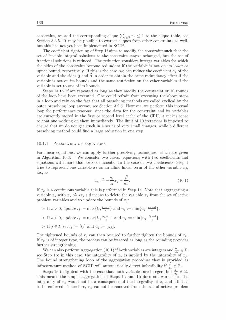
136 Presolving
constraint, we add the corresponding clique∑
j∈S xj ≤ 1 to the clique table, seeSection 3.3.5. It may be possible to extract cliques from other constraints as well,but this has not yet been implemented in SCIP.
The coefficient tightening of Step 1f aims to modify the constraint such that theset of feasible integral solutions to the constraint stays unchanged, but the set offractional solutions is reduced. The reduction considers integer variables for whichthe sides of the constraint become redundant if the variable is not on its lower orupper bound, respectively. If this is the case, we can reduce the coefficient aj of thevariable and the sides β and β in order to obtain the same redundancy effect if thevariable is not on its bounds and the same restriction on the other variables if thevariable is set to one of its bounds.
Steps 1a to 1f are repeated as long as they modify the constraint or 10 roundsof the loop have been executed. One could refrain from executing the above stepsin a loop and rely on the fact that all presolving methods are called cyclical by theouter presolving loop anyway, see Section 3.2.5. However, we perform this internalloop for performance reasons: since the data for the constraint and its variablesare currently stored in the first or second level cache of the CPU, it makes senseto continue working on them immediately. The limit of 10 iterations is imposed toensure that we do not get stuck in a series of very small changes, while a differentpresolving method could find a large reduction in one step.
10.1.1 Presolving of Equations
For linear equations, we can apply further presolving techniques, which are givenin Algorithm 10.3. We consider two cases: equations with two coefficients andequations with more than two coefficients. In the case of two coefficients, Step 1tries to represent one variable xk as an affine linear term of the other variable xj ,i.e., as
xk :⋆= −
aj
ak
xj +β
ak
. (10.1)
If xk is a continuous variable this is performed in Step 1a. Note that aggregating avariable xk with xk : ⋆= sxj +d means to delete the variable xk from the set of activeproblem variables and to update the bounds of xj :
⊲ If s > 0, update lj := max{lj ,lk−d
s} and uj := min{uj ,
uk−ds}.
⊲ If s < 0, update lj := max{lj ,uk−d
s} and uj := min{uj ,
lk−ds}.
⊲ If j ∈ I, set lj := ⌈lj⌉ and uj := ⌊uj⌋.
The tightened bounds of xj can then be used to further tighten the bounds of xk.If xk is of integer type, the process can be iterated as long as the rounding providesfurther strengthening.
We can also perform Aggregation (10.1) if both variables are integers andaj
ak∈ Z,
see Step 1b; in this case, the integrality of xk is implied by the integrality of xj .The bound strengthening loop of the aggregation procedure that is provided as
infrastructure method of SCIP will automatically detect infeasibility if βak
/∈ Z.
Steps 1c to 1g deal with the case that both variables are integers butaj
ak/∈ Z.
This means the simple aggregation of Steps 1a and 1b does not work since theintegrality of xk would not be a consequence of the integrality of xj and still hasto be enforced. Therefore, xk cannot be removed from the set of active problem
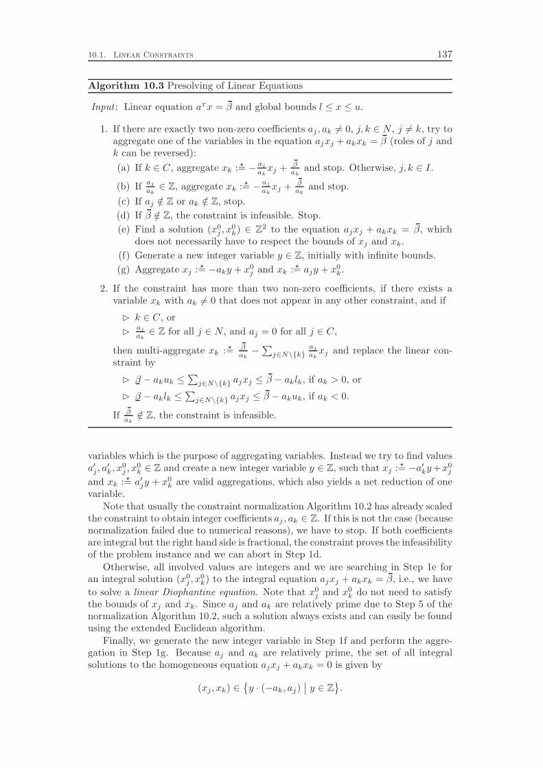
10.1. Linear Constraints 137
Algorithm 10.3 Presolving of Linear Equations
Input : Linear equation aTx = β and global bounds l ≤ x ≤ u.
1. If there are exactly two non-zero coefficients aj , ak 6= 0, j, k ∈ N , j 6= k, try toaggregate one of the variables in the equation ajxj + akxk = β (roles of j andk can be reversed):
(a) If k ∈ C, aggregate xk : ⋆= − aj
akxj + β
akand stop. Otherwise, j, k ∈ I.
(b) Ifaj
ak∈ Z, aggregate xk : ⋆= −
aj
akxj + β
akand stop.
(c) If aj /∈ Z or ak /∈ Z, stop.
(d) If β /∈ Z, the constraint is infeasible. Stop.
(e) Find a solution (x0j , x
0k) ∈ Z2 to the equation ajxj + akxk = β, which
does not necessarily have to respect the bounds of xj and xk.
(f) Generate a new integer variable y ∈ Z, initially with infinite bounds.
(g) Aggregate xj : ⋆= −aky + x0j and xk : ⋆= ajy + x0
k.
2. If the constraint has more than two non-zero coefficients, if there exists avariable xk with ak 6= 0 that does not appear in any other constraint, and if
⊲ k ∈ C, or
⊲aj
ak∈ Z for all j ∈ N , and aj = 0 for all j ∈ C,
then multi-aggregate xk : ⋆= βak−∑
j∈N\{k}aj
akxj and replace the linear con-
straint by
⊲ β − akuk ≤∑
j∈N\{k} ajxj ≤ β − aklk, if ak > 0, or
⊲ β − aklk ≤∑
j∈N\{k} ajxj ≤ β − akuk, if ak < 0.
If βak
/∈ Z, the constraint is infeasible.
variables which is the purpose of aggregating variables. Instead we try to find valuesa′j , a
′k, x
0j , x
0k ∈ Z and create a new integer variable y ∈ Z, such that xj : ⋆= −a′ky+x0
j
and xk : ⋆= a′jy + x0k are valid aggregations, which also yields a net reduction of one
variable.Note that usually the constraint normalization Algorithm 10.2 has already scaled
the constraint to obtain integer coefficients aj , ak ∈ Z. If this is not the case (becausenormalization failed due to numerical reasons), we have to stop. If both coefficientsare integral but the right hand side is fractional, the constraint proves the infeasibilityof the problem instance and we can abort in Step 1d.
Otherwise, all involved values are integers and we are searching in Step 1e foran integral solution (x0
j , x0k) to the integral equation ajxj + akxk = β, i.e., we have
to solve a linear Diophantine equation. Note that x0j and x0
k do not need to satisfythe bounds of xj and xk. Since aj and ak are relatively prime due to Step 5 of thenormalization Algorithm 10.2, such a solution always exists and can easily be foundusing the extended Euclidean algorithm.
Finally, we generate the new integer variable in Step 1f and perform the aggre-gation in Step 1g. Because aj and ak are relatively prime, the set of all integralsolutions to the homogeneous equation ajxj + akxk = 0 is given by
(xj , xk) ∈{y · (−ak, aj)
∣∣ y ∈ Z
}.
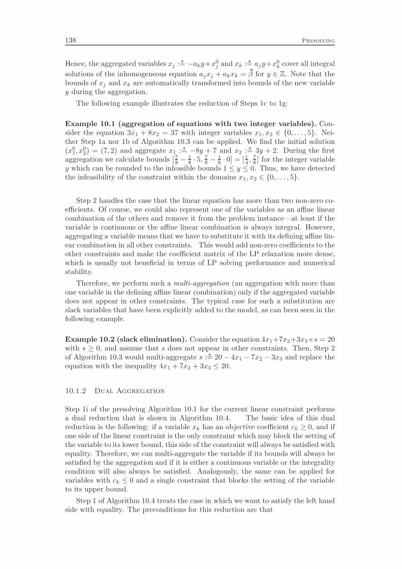
138 Presolving
Hence, the aggregated variables xj : ⋆= −aky+x0j and xk : ⋆= ajy+x0
k cover all integral
solutions of the inhomogeneous equation ajxj + akxk = β for y ∈ Z. Note that thebounds of xj and xk are automatically transformed into bounds of the new variabley during the aggregation.
The following example illustrates the reduction of Steps 1c to 1g:
Example 10.1 (aggregation of equations with two integer variables). Con-sider the equation 3x1 + 8x2 = 37 with integer variables x1, x2 ∈ {0, . . . , 5}. Nei-ther Step 1a nor 1b of Algorithm 10.3 can be applied. We find the initial solution(x0
1, x02) = (7, 2) and aggregate x1 : ⋆= −8y + 7 and x2 : ⋆= 3y + 2. During the first
aggregation we calculate bounds [78− 1
8· 5, 7
8− 1
8· 0] = [1
4, 7
8] for the integer variable
y which can be rounded to the infeasible bounds 1 ≤ y ≤ 0. Thus, we have detectedthe infeasibility of the constraint within the domains x1, x2 ∈ {0, . . . , 5}.
Step 2 handles the case that the linear equation has more than two non-zero co-efficients. Of course, we could also represent one of the variables as an affine linearcombination of the others and remove it from the problem instance—at least if thevariable is continuous or the affine linear combination is always integral. However,aggregating a variable means that we have to substitute it with its defining affine lin-ear combination in all other constraints. This would add non-zero coefficients to theother constraints and make the coefficient matrix of the LP relaxation more dense,which is usually not beneficial in terms of LP solving performance and numericalstability.
Therefore, we perform such a multi-aggregation (an aggregation with more thanone variable in the defining affine linear combination) only if the aggregated variabledoes not appear in other constraints. The typical case for such a substitution areslack variables that have been explicitly added to the model, as can been seen in thefollowing example.
Example 10.2 (slack elimination). Consider the equation 4x1+7x2+3x3+s = 20with s ≥ 0, and assume that s does not appear in other constraints. Then, Step 2of Algorithm 10.3 would multi-aggregate s : ⋆= 20− 4x1 − 7x2 − 3x3 and replace theequation with the inequality 4x1 + 7x2 + 3x3 ≤ 20.
10.1.2 Dual Aggregation
Step 1i of the presolving Algorithm 10.1 for the current linear constraint performsa dual reduction that is shown in Algorithm 10.4. The basic idea of this dualreduction is the following: if a variable xk has an objective coefficient ck ≥ 0, and ifone side of the linear constraint is the only constraint which may block the setting ofthe variable to its lower bound, this side of the constraint will always be satisfied withequality. Therefore, we can multi-aggregate the variable if its bounds will always besatisfied by the aggregation and if it is either a continuous variable or the integralitycondition will also always be satisfied. Analogously, the same can be applied forvariables with ck ≤ 0 and a single constraint that blocks the setting of the variableto its upper bound.
Step 1 of Algorithm 10.4 treats the case in which we want to satisfy the left handside with equality. The preconditions for this reduction are that

10.1. Linear Constraints 139
Algorithm 10.4 Dual Aggregation for Linear Constraints
Input : Linear constraint β ≤ aTx ≤ β.
1. If β > −∞ and there is a variable xk with
(a) β − αk ≥ min{aklk, akuk},
(b) β − αk ≤ max{aklk, akuk},
(c) with
⊲ k ∈ C or⊲
aj
ak∈ Z for all j ∈ N and aj = 0 for all j ∈ C,
(d) and with
⊲ ak > 0, ck ≥ 0, and ζ−k = 1, or⊲ ak < 0, ck ≤ 0, and ζ+
k = 1,
aggregate xk : ⋆= β
ak−∑
j 6=kaj
akxj and delete the constraint. If k ∈ I and
β
ak/∈ Z, the constraint is infeasible.
2. If β < +∞ and there is a variable xk with
(a) β − αk ≥ min{aklk, akuk},
(b) β − αk ≤ max{aklk, akuk},
(c) with
⊲ k ∈ C or⊲
aj
ak∈ Z for all j ∈ N and aj = 0 for all j ∈ C,
(d) and with
⊲ ak > 0, ck ≤ 0, and ζ+k = 1, or
⊲ ak < 0, ck ≥ 0, and ζ−k = 1,
aggregate xk : ⋆= βak−∑
j 6=kaj
akxj and delete the constraint. If k ∈ I and
βak
/∈ Z, the constraint is infeasible.
1. the resulting aggregation
xk :⋆=
β
ak
−∑
j 6=k
aj
ak
xj
satisfies the bounds of xk for all values of xj , j 6= k (Conditions 1a and 1b),
2. either the variable is continuous or the aggregation is always integral (Condi-tion 1c), and
3. the constraint at hand is the only constraint that blocks the setting of thevariable to its best bound w.r.t. the objective function (Condition 1d).
Recall that the variable lock numbers ζ−k and ζ+k queried in Condition 1d denote
the number of constraints that block the shifting of the variable in the respectivedirection, compare Definition 3.3 on page 38. For β > −∞, the conditions ak > 0and ak < 0 state that this constraint locks the variable in the corresponding directionand is therefore the reason for ζ−k = 1 or ζ+
k = 1, respectively.Step 2 treats the case where we want to satisfy the right hand side of the con-
straint with equality. It applies the same reasoning as Step 1.

140 Presolving
10.1.3 Presolving of Constraint Pairs
After the individual constraint presolving in Step 1 of Algorithm 10.1 has been ap-plied, the presolving continues with processing pairs of linear constraints as depictedin Algorithm 10.5. Since this pairwise comparison of constraints is quite expensivewith its worst case runtime of O(nm2) for dense coefficient matrices, we only applyit if no presolving method in the current presolving round found a reduction. Thefirst step of the pairwise presolving algorithm is to calculate positive and negativesignatures for all constraints. These are defined as follows:
Definition 10.3 (constraint signatures). Let Ci : β ≤ aTx ≤ β be a linearconstraint. Then, the bit vectors sig+
i , sig−i ∈ {0, 1}
64 with
(sig+i )k =
{
1 if ∃j ∈ N : max{ajlj , ajuj} > 0 ∧ (j mod 64) = k,
0 otherwise
(sig−i )k =
{
1 if ∃j ∈ N : min{ajlj , ajuj} < 0 ∧ (j mod 64) = k,
0 otherwise
for k = 0, . . . , 63 are called positive and negative signatures of constraint Ci.
The signatures are used in the remaining algorithm to quickly rule out unin-teresting pairs of constraints where no presolving reduction can be applied. Notethat they can be stored in 64 bit registers, and fast bit instructions can be used tocompare the signature vectors of two constraints. Our experience is (although notsupported with detailed computational results) that—with deactivated constraintaggregation, see below—this signature filter suffices to discard almost all constraintpairs on which no presolving can be applied, which significantly reduces the runningtime of the algorithm.
After calculating the signatures, we proceed with the pairwise comparison loopin Step 2. We perform a bookkeeping on the constraint modifications which allowsus to skip pairs for which none of the two constraints has been altered since the lastcall to the comparison algorithm.
Step 2a compares the signatures and the sides of the constraints to check whetherreductions are possible. This is the case if the constraint coefficients are equal(potentially after multiplying one of the constraints with−1), if one of the constraintsdominates one of the sides, or if at least one of the constraints is an equation, whichmay yield the possibility to aggregate the constraints. If the positive and negativesignatures of the constraints differ, the coefficients cannot be equal. If the positivesignature of one constraint differs from the negative signature of the other constraint,the coefficients cannot be negated versions of each other. The domination of the leftand right hand sides is defined as follows:
Definition 10.4 (domination of constraint sides). Let Cp : βp ≤ (ap)Tx ≤ βp
and Cq : βq ≤ (aq)Tx ≤ βq be a pair of linear constraints defined on variablesx ∈ [l, u], l, u ∈ R∪{±∞}. Then we say that the left hand side of Cp dominates thethe left hand side of Cq, if
βp ≥ βq and ∀j ∈ N ∀xj ∈ [lj , uj ] : apjxj ≤ a
qjxj .
The right hand side of Cp dominates the right hand side of Cq, if
βp ≤ βq and ∀j ∈ N ∀xj ∈ [lj , uj ] : apjxj ≥ a
qjxj .

10.1. Linear Constraints 141
Algorithm 10.5 Pairwise Presolving of Linear Constraints
1. For all linear constraints Ci calculate the signature vectors sig+i , sig
−i ∈ {0, 1}
64.
2. For all pairs (Cp, Cq), p < q, of linear constraints where at least one of the twohas been modified since the last call to Algorithm 10.5:
(a) Compare the signatures to check whether reductions are possible:
coefseq := (sig+p = sig+
q )∧ (sig−p = sig−q )
coefsneg := (sig+p = sig−q )∧ (sig−p = sig+
q )
lhsdomp := (βp ≥ βq) ∧ (sig+p ≤ sig+
q )∧ (sig−p ≥ sig+q )
lhsdomq := (βp ≤ βq) ∧ (sig+p ≥ sig+
q )∧ (sig−p ≤ sig+q )
rhsdomp := (βp ≤ βq) ∧ (sig+p ≥ sig+
q )∧ (sig−p ≤ sig+q )
rhsdomq := (βp ≥ βq) ∧ (sig+p ≤ sig+
q )∧ (sig−p ≥ sig+q )
aggr := (βp = βp) ∨ (βq = βq)
If all of these Boolean values are 0, continue Loop 2 with the next pair.
(b) For all j ∈ N , as long as one of the Boolean values of Step 2a is 1:
i. If apj 6= aq
j , set coefseq := 0.ii. If ap
j 6= −aqj , set coefsneg := 0.
iii. If apj > aq
j and lj < 0 set rhsdomp := 0 and lhsdomq := 0.iv. If ap
j > aqj and uj > 0 set lhsdomp := 0 and rhsdomq := 0.
v. If apj < aq
j and lj < 0 set lhsdomp := 0 and rhsdomq := 0.vi. If ap
j < aqj and uj > 0 set rhsdomp := 0 and lhsdomq := 0.
(c) If lhsdomp = 1, set βq := −∞. Else, if lhsdomq = 1, set βp := −∞.If rhsdomp = 1, set βq := +∞. Else, if rhsdomq = 1, set βp := +∞.
(d) If βp = −∞ and βp = +∞, delete Cp and continue Loop 2.If βq = −∞ and βq = +∞, delete Cq and continue Loop 2.
(e) If coefseq = 1, set βp := max{βp, βq}, βp := min{βp, βq}, delete Cq, andcontinue Loop 2.If coefsneg = 1, set βp := max{βp,−βq}, βp := min{βp,−βq}, delete Cq,and continue Loop 2.
(f) If βp = βp, select k ∈ N to minimize
ω⋆ := min
{
ω(
aq −aq
k
apk
ap)
| k ∈ N : apk, a
qk ∈ Z \ {0}
}
.
If ω⋆ < ω(aq) and∥∥aq
j −a
q
k
ap
k
ap∥∥∞≤∥∥aq
j
∥∥∞
, replace Cq with Cq −a
q
k
ap
k
Cp,
i.e., with
βq −aq
k
apk
βp ≤(
aq −aq
k
apk
ap)T
x ≤ βq −aq
k
apk
βp.
(g) If βp 6= βp and βq = βq, perform an analogous calculation as in Step 2f
to replace Cp with Cp −a
p
k
aq
k
Cq.
142 Presolving
The following is a simple reformulation of the domination definition:
Observation 10.5. For constraints defined as in Definition 10.4 the following holds:
1. βp dominates βq if and only if βp ≥ βq and
∀j ∈ N :((lj < 0→ ap
j ≥ aqj) ∧ (uj > 0→ ap
j ≤ aqj )).
2. βp dominates βq if and only if βp ≤ βq and
∀j ∈ N :((lj < 0→ ap
j ≤ aqj) ∧ (uj > 0→ ap
j ≥ aqj )).
The purpose of identifying constraint side dominations is to remove a redundantside by applying the following proposition:
Proposition 10.6. Let Cp and Cq be defined as in Definition 10.4. Let C−∞q :
−∞ ≤ (aq)Tx ≤ βq and C+∞q : βq ≤ (aq)Tx ≤ +∞ be relaxations of Cq, and defineC := {Cp, Cq}, C−∞ := {Cp, C
−∞q }, and C+∞ := {Cp, C
+∞q }. Then the following
holds:
1. If βp dominates βq, then C(x) = C−∞(x) for all x ∈ [l, u].
2. If βp dominates βq, then C(x) = C+∞(x) for all x ∈ [l, u].
Proof. Recall that the function C(x) : Rn → {0, 1} maps to 1 if and only if x satisfiesall constraints C ∈ C. Thus, in order to prove Statement 1 we have to show that theset of vectors which satisfy both constraints does not change if the left hand side ofCq is replaced by −∞. Since C−∞ is a relaxation of C, C(x) = 1 implies C−∞(x) = 1for all x ∈ [l, u]. To show the other direction, consider an arbitrary vector x ∈ [l, u]with C−∞(x) = 1. Then,
∑
j∈N
aqjxj ≥
∑
j∈N
apjxj ≥ βp ≥ βq
holds as a direct consequence of Definition 10.4. Therefore, Cq is satisfied and wehave C(x) = 1. Statement 2 can be shown analogously.
The constraint signatures may give a simple proof for the non-dominance of thesides: if there is a potentially positive summand ajxj in Cp for which the corres-ponding summand in Cq is always non-positive, or if there is a potentially negativesummand in Cq for which the corresponding summand in Cp is always non-negative,constraint Cp cannot dominate the left hand side. Analogous reasoning applies tothe other domination relations.
If the signatures allow for a reduction, we proceed with Step 2b, which comparesthe individual coefficients in the constraint to check exactly whether one of thepossible reductions can be applied. If applicable, the removal of redundant sides isperformed in Step 2c. If this resulted in a constraint with both sides being infinite,the constraint is deleted in Step 2d. If the coefficients of the constraints are eitherpairwise equal or pairwise negated, we can replace the two constraints by a singleconstraint. This means in particular that equations and ranged rows that have beendisaggregated by the modeler are aggregated again into a single constraint.
10.1. Linear Constraints 143
Algorithm 10.6 Dual Bound Reduction for Linear Constraints
1. Calculate redundancy bounds redlj and reduj for all j ∈ N .
2. For all variables j ∈ N :
(a) If cj ≥ 0 and xj is only down-locked by linear constraints, update uj :=min{uj , redlj}.
(b) If cj ≤ 0 and xj is only up-locked by linear constraints, update lj :=max{lj , reduj}.
Steps 2f and 2g add an equation to the other constraint in order to reduce theweighted support of the constraint. We define the weighted support of a linearconstraint to be
ω(a) =∣∣{j ∈ B | aj 6= 0}
∣∣
+4∣∣{j ∈ I \B | aj 6= 0}
∣∣
+8∣∣{j ∈ C | aj 6= 0}
∣∣,
i.e., each binary variable in the constraint counts as 1, each general integer variableas 4, and each continuous variable counts as 8. The goal is to reduce the numberof non-zero entries, in particular the ones that belong to non-binary variables. Thiscan be useful to upgrade the constraint to a more specific type in Step 4 of Algo-rithm 10.1. The additional hope is that it also helps the aggregation heuristic ofthe complemented mixed integer rounding cut separator to find more cuts, and toenable the generation of flow cover cuts, see Sections 8.2 and 8.5.
For numerical reasons, we restrict the aggregation to apply the coefficient elimi-nation only on those variables where both coefficients ap
k and aqk have integral values.
Additionally, we do not want the maximum norm of the coefficient vector to increase,since this may also lead to numerical issues, in particular after many aggregationsapplied to the same constraint. Note, however, that this aggregation of constraintsis disabled in the default settings of SCIP. Without aggregation, Algorithm 10.5can usually be executed much faster, since then we can ignore the aggr variable inStep 2a, which makes it more likely to skip the constraint pair.
10.1.4 Dual Bound Reduction
In Step 3 of the presolving Algorithm 10.1 for linear constraints, we perform an-other dual reduction that can be applied to all variables that only appear in linearconstraints. Algorithm 10.6 illustrates the procedure.
Step 1 calculates so-called redundancy bounds for each variable j ∈ N , which aredefined as follows:
Definition 10.7 (redundancy bounds). Given a set C = {C1, . . . , Cm} of linearconstraints Ci : βi ≤ (ai)Tx ≤ βi, the values redlj , reduj ∈ R ∪ {±∞} defined as
redlj := min{xj ∈ R | αij + ai
jxj ≥ βi for all Ci with aij > 0 and
αij + ai
jxj ≤ βi for all Ci with aij < 0}
reduj := max{xj ∈ R | αij + ai
jxj ≥ βi for all Ci with aij < 0 and
αij + ai
jxj ≤ βi for all Ci with aij > 0}
144 Presolving
are called redundancy bounds of variable j w.r.t. the linear constraints C. Here, αij
and αij are the activity bound residuals of (ai)Tx w.r.t. xj , see Definition 7.1 on
page 83.
The purpose of calculating these values becomes clear with the following simpleproposition:
Proposition 10.8. Let C be a set of linear constraints that only have one finite sideβ or β each, and let j ∈ N . Then the following holds:
1. All constraints Ci ∈ C that down-lock variable xj are redundant if xj ≥ redlj .
2. All constraints Ci ∈ C that up-lock variable xj are redundant if xj ≤ reduj .
Proof. Consider the inequality β ≤ aTx and assume aj > 0. Then, this constraintdown-locks variable xj , compare Definition 3.3 on page 38. For xj ≥ redlj we haveαj + ajxj ≥ β by Definition 10.7. This is equivalent to
∀{x ∈ [l, u] | xj ≥ redlj} : aTx ≥ β,
which means that the constraint is redundant if xj ≥ redlj . The remaining casescan be shown analogously.
Proposition 10.8 is applied in Step 2 of Algorithm 10.6. If the objective coeffi-cient cj is non-negative and all constraints that become “less feasible” by decreasingxj are already redundant for xj ≥ redlj , then there is no reason to set xj to a largervalue than redlj . In other words, if the problem instance is feasible and bounded,there is always an optimal solution x⋆ with x⋆
j ≤ redlj . Therefore, we can tightenthe upper bound in Step 2a and still preserve at least one optimal solution. Step 2bis analogous.
10.1.5 Upgrading of Linear Constraints
The final Step 4 of the main presolving Algorithm 10.1 is to upgrade linear con-straints into constraints of a more specific type. For this, the linear constrainthandler provides a callback mechanism which other constraint handlers can use totake over linear constraints and convert them into equivalent constraints of their owntype. The linear constraint handler calculates certain statistics for each constraintin order to simplify the upgrading process for the other constraint handlers. This isshown in Algorithm 10.7.
First, we call the normalization Algorithm 10.2 another time, since the constraintmight have been modified since the last normalization in Step 1a of Algorithm 10.1.Then, we calculate a number of statistical values for the constraint, namely the num-ber of positive and negative coefficients for binary, general integer, and continuousvariables, the number of ±1 coefficients, and the number of positive and negativeintegral and fractional coefficients. Finally, the upgrade methods of the constrainthandlers that are hooked to the linear constraint upgrading mechanism are called ina specified order, see below. The first constraint handler that calls for the constrainttransforms it into one of its own type, and the linear representation of the constraintis deleted.
The upgrade methods of other constraint handlers can use the calculated statis-tics, but can also consider the coefficient vector and left and right hand sides directly.
10.1. Linear Constraints 145
Algorithm 10.7 Upgrading of Linear Constraints
Input : Linear constraint β ≤ aTx ≤ β.
1. Call Algorithm 10.2 to normalize the constraint.
2. Calculate the following statistics:
nvars := |{j ∈ N | aj 6= 0}|
nposbin := |{j ∈ B | aj > 0}|
nnegbin := |{j ∈ B | aj < 0}|
nposgenint := |{j ∈ I \B | aj > 0}|
nneggenint := |{j ∈ I \B | aj < 0}|
nposcont := |{j ∈ C | aj > 0}|
nnegcont := |{j ∈ C | aj < 0}|
nposcoefone := |{j ∈ N | aj = 1}|
nnegcoefone := |{j ∈ N | aj = −1}|
nposcoefint := |{j ∈ N | aj ∈ Z>0 \ {1}}|
nnegcoefint := |{j ∈ N | aj ∈ Z<0 \ {−1}}|
nposcoeffrac := |{j ∈ N | aj ∈ R>0 \ Z}|
nnegcoeffrac := |{j ∈ N | aj ∈ R<0 \ Z}|
3. Call all registered constraint handlers in the given priority order until one ofthem took over the constraint. If successful, delete the linear constraint.
However, all constraint handlers for special types of linear constraints available inSCIP can decide the membership of the constraint to their class by inspecting thestatistics only. They are called in the following order and verify the given statis-tics. Note that the tests check whether it is possible to reach the standard formof the constraint by complementing some of the binary variables and optionally bymultiplying the constraint with −1.
1. set covering constraints:∑
j∈S xj ≥ 1 with S ⊆ B
⊲ nposbin + nnegbin = nvars,
⊲ nposcoefone + nnegcoefone = nvars,
⊲ β = 1− nnegcoefone or β = nposcoefone− 1, and
⊲ β = −∞ or β = +∞.
2. set packing constraints:∑
j∈S xj ≤ 1 with S ⊆ B
⊲ nposbin + nnegbin = nvars,
⊲ nposcoefone + nnegcoefone = nvars,
⊲ β = nposcoefone− 1 or β = 1− nnegcoefone, and
⊲ β = −∞ or β = +∞.
3. set partitioning constraints:∑
j∈S xj = 1 with S ⊆ B
146 Presolving
⊲ nposbin + nnegbin = nvars,
⊲ nposcoefone + nnegcoefone = nvars, and
⊲ β = β = nposcoefone− 1 or β = β = 1− nnegcoefone.
4. knapsack constraints: aTx ≤ β with aj ∈ Z≥0 for j ∈ B, aj = 0 for j ∈ N \B,and β ∈ Z≥0
⊲ nposbin + nnegbin = nvars,
⊲ nposcoefone + nnegcoefone + nposcoefint + nnegcoefint = nvars, and
⊲ β = −∞ or β = +∞.
5. variable bound constraints: β ≤ xi + ajxj ≤ β with i ∈ N \B and j ∈ I
⊲ nvars = 2,
⊲ nposbin + nnegbin ≤ 1, and
⊲ nposcont + nnegcont ≤ 1.
Note that the knapsack constraint handler does not need to check whether theresulting right hand side after transforming the coefficients into a ∈ Z≥0 is integraland non-negative. This is already ensured by the presolving of linear constraints,compare Steps 1b and 1d of Algorithm 10.1.
10.2 Knapsack Constraints
A binary knapsack constraint is a linear constraint
aTx ≤ β
with a ∈ ZB≥0, xj ∈ {0, 1} for j ∈ B, and β ∈ Z≥0. The coefficients aj are called
weights, the right hand side β is called capacity of the knapsack.To transform a linear inequality on binary variables with integral coefficients
into a knapsack constraint, it is sometimes necessary to complement some of thebinary variables using xj = 1 − xj . If we want to access or modify the weight ofa negated variable xj , we write aj . In terms of the active problem variables, sucha “complemented” coefficient means to have a negative coefficient aj = −aj and
an updated right hand side β − aj . However, it is easier to think of xj and xj asbeing two different variables with both having non-negative coefficients. For ease ofnotation, we assume that there are no complemented variables in the initial form ofthe knapsack constraint.
Presolving for knapsack constraints is much easier than for linear constraints.On the one hand, we can usually rely on the fact that all presolving methods of thelinear constraint handler have already been applied and the constraint was upgradedinto a knapsack constraint afterwards. On the other hand, knapsack constraints aremuch simpler, since they are pure inequalities that consist of only binary variablesand non-negative integral coefficients. There is one ingredient implemented inthe knapsack presolving algorithm, however, that is not available for general linearconstraints, at least not in the SCIP implementation: coefficient tightening andlifting using clique information.

10.2. Knapsack Constraints 147
Algorithm 10.8 Presolving for Knapsack Constraints
Input : Knapsack constraint aTx ≤ β with item set S := {j ∈ N | aj > 0}.
1. Remove fixed variables: if lj = uj , set β := β − aj lj , and aj := 0.
2. Calculate d := gcd(a), and set aj := aj/d and β := ⌊β/d⌋.
3. Tighten the bounds of the variables by calling the domain propagation Algo-rithm 7.3. Remove variables from S that have been fixed to zero.
4. Sort the item set S = {j1, . . . , jp} by non-increasing weight aj1 ≥ . . . ≥ ajp.
5. Let k be the largest position in S = {j1, . . . , jp} with ajk+ ajk+1
> β. If kexists, then do for all l = k + 1, . . . , p:
(a) If ajk+ajl
> β add the clique xj1 + . . .+xjk+xjl
≤ 1 to the clique table.
6. Let α := aT1. For all k = 1, . . . , p:
(a) If αjk:= α− ajk
≥ β, break the loop.
(b) Set ∆ := β − αjk, ajk
:= ajk−∆, β := β −∆, and α := α−∆.
7. Partition S into pairwise disjoint cliques S = Q1 ∪ . . . ∪ Qq using a greedyalgorithm. For each clique Ql let aQl
:= max{aj | j ∈ Ql} be the maximumweight in the clique, and let αQ :=
∑ql=1 aQl
be the sum of the maximumclique weights. Sort the cliques by non-increasing aQl
. For all l = 1, . . . , q:
(a) If αQQl
:= αQ − aQl≥ β, break the loop.
(b) Set ∆ := β − αQQl
, aj := max{aj −∆, 0} for all j ∈ Ql, β := β −∆, and
αQ := αQ −∆.
(c) If min{aj + ak | j, k ∈ Ql, j 6= k} ≤ β, add set packing constraint∑
j∈Qlxj ≤ 1 to the problem instance.
Update S to account for the coefficients which have been set to zero.
8. For all binary variables xk, k ∈ B, and values v ∈ {0, 1}:
(a) Calculate the clique residuals Cxk=vl := Cl \ {j ∈ Cl | xk = v → xj = 0}
for all cliques Cl, l = 1, . . . , q, in the clique partition of S.
(b) Let aQxk=v
l:= max{aj | j ∈ Q
xk=vl } be the maximum weight in the clique
residual, and let αQxk=v
:=∑q
l=1 aQxk=v
lbe the sum of the maximum
clique residual weights.
(c) If αQxk=v
< β, set q := q + 1, ∆ := β − αQxk=v
and
i. if v = 1, set ak := ak + ∆, Qq := {k}, and update S := S ∪ {k},ii. if v = 0, set ak := ak + ∆, Qq := {k}, and update S := S ∪ {k} with
ak being the coefficient for the complemented variable xk of xk.
9. For all pairs of complemented variables k, k ∈ S:
(a) If ak > ak, set β := β − ak, ak := ak − ak, ak := 0, and S := S \ {k}.
(b) If ak < ak, set β := β − ak, ak := ak − ak, ak := 0, and S := S \ {k}.
(c) If ak = ak, set β := β − ak, ak := 0, ak := 0, and S := S \ {k, k}.
10. Sort item set S by non-increasing weight aj : S = {j1, . . . , jq}.For all k = 1, . . . , q − 1:
(a) If ajk+ ajq
≤ β, break the loop.
(b) Set ajk:= β. If k = q − 1, set ajq
:= β.
148 Presolving
Algorithm 10.8 describes the proceeding of the presolving for a single knapsackconstraint, which is successively applied to all knapsack constraints of the probleminstance. Step 1 cleans up the constraint data by removing all fixed variablesfrom the constraint. If a variable is fixed to 1, its weight has to be subtracted fromthe capacity. Note that additionally, all variables are replaced by their uniquerepresentative, which is either an active problem variable xj , or the negation xj ofan active problem variable. In Step 2, the weights are divided by their greatestcommon divisor. Of course, the capacity has to be divided by the same value, andit can be rounded down afterwards.
In Step 3, we tighten the bounds of the variables by calling the domain propaga-tion Algorithm 7.3 on page 90 and clean up the item set by removing the variablesthat have been fixed to zero in the propagation.
10.2.1 Clique Extraction
As all constraints in SCIP, a knapsack constraint is internally represented in a sparsefashion, i.e., only the non-zero coefficients and their corresponding indices are stored.The set S denotes this index set, and we make sure in Step 4 that it is stored in anorder of non-increasing weights aj . Then in Step 5, it is easy to extract all maximalcliques induced by the knapsack constraint in order to add them to the clique tableof SCIP: they always consist of the variables with the k largest coefficients and oneadditional variable.
Definition 10.9 (maximal induced clique). Let C : Rn → {0, 1} be a constrainton variables xj , j ∈ N , and let B ⊆ N be the subset of binary variables. Then,Q ⊆ B is called induced clique of C if
C(x) = 1 ⇒∑
j∈Q
xj ≤ 1.
An induced clique Q of C is called maximal induced clique of C if
C(x) = 1 6⇒∑
j∈Q∪{q}
xj ≤ 1
for all q ∈ B \Q.
Proposition 10.10 (maximal induced cliques of knapsacks). Let aTx ≤ β bea knapsack constraint on binary variables xj , j ∈ S := {1, . . . , p} ⊆ B, with positiveintegral coefficients a1 ≥ . . . ≥ ap and a1 ≤ β. Then, Q ⊆ S with |Q| ≥ 2 is amaximal induced clique of the knapsack constraint if and only if
1. Q = {1, . . . , k} ∪ {l} with 1 ≤ k < l ≤ p,
2. ak + al > β, and
3. k = p− 1 or ak+1 + ak+2 ≤ β.
Proof. Let Q = {1, . . . , k} ∪ {l}, 1 ≤ k < l ≤ p, with ak + al > β. Then, for alli, j ∈ Q, i 6= j, we have
ai + aj ≥ ak + al > β,
which means that all variables in Q are pairwise contradictory and Q is a clique. Ifk = p− 1 then Q = S, and the clique is maximal because due to a1 ≤ β no variable
10.2. Knapsack Constraints 149
j ∈ B \ S (i.e., aj = 0) can be a member of an induced clique. Otherwise, assumeak+1 + ak+2 ≤ β, and suppose that Q is not a maximal induced clique. Then, thereexists l′ ∈ S \Q with aj + al′ > β for all j ∈ Q. In particular, al + al′ > β. Froml′ ∈ S \Q and Q = {1, . . . , k} ∪ {l} it follows that either l = k + 1 and l′ ≥ k + 2 orl ≥ k + 2 and l′ ≥ k + 1. In both cases we have
β < al + al′ ≤ ak+1 + ak+2 ≤ β,
which is a contradiction. This completes the proof of the maximality of clique Q.To prove the other direction of the proposition, assume that Q is a maximal
induced clique of the knapsack constraint and there are more than two variablesafter the first “hole” in the index set Q, i.e., there exist k ∈ S \Q and l, l′ ∈ Q withk < l < l′. Since Q is an induced clique, we have aj + al′ > β for all j ∈ Q \ {l′}. Itfollows that
aj + ak ≥ aj + al′ > β
for all j ∈ Q \ {l′} andak + al′ ≥ al + al′ > β.
Therefore, Q ∪ {k} is an induced clique, which contradicts the maximality of Q.Thus, Condition 1 holds. Condition 2 holds because Q is a clique, and Condition 3follows from the maximality of Q.
10.2.2 Coefficient Tightening
Steps 6 and 7 of Algorithm 10.8 tighten the weights of the knapsack constraint,which means to modify the weights and the capacity such that the set of feasibleintegral solutions to the knapsack constraint stays unaffected, but the LP relaxationis improved.
Step 6 performs the easy modifications that are already justified only by theweights and capacity. If the sum of all weights except ak is at most the capacityβ, the constraint is redundant for xk = 0. If this sum αk is smaller than β, wecan decrease the weight and the capacity by the difference ∆ = β − αk, since then,the constraint is also redundant for xk = 0, and it has the same remaining capacityβ−ak for xk = 1. However, the LP relaxation becomes stronger: if all other variablesj 6= k are set to xj = 1, the LP value of xk is forced to be 0 instead of having the
possibility to be anywhere in[0, β−αk
ak
].
Example 10.11 (coefficient tightening for knapsacks). Consider the knapsackconstraint
12x1 + 10x2 + 7x3 + 7x4 + 5x5 + 4x6 + 3x7 + x8 ≤ 42.
The sum of all weights is α = 49. The maximal residual activity bound for x1 isα1 = 49−12 = 37 < 42. Therefore, we can reduce a1 and β by 42−37 = 5 to obtain
7x1 + 10x2 + 7x3 + 7x4 + 5x5 + 4x6 + 3x7 + x8 ≤ 37
and an updated weight sum of α = 44. For the next item x2, the maximal residualactivity bound is α2 = 44− 10 = 34 < 37. We can reduce a2 and β by 37 − 34 = 3to obtain
7x1 + 7x2 + 7x3 + 7x4 + 5x5 + 4x6 + 3x7 + x8 ≤ 34.
For x3 we have α3 = 41− 7 = 34 = β and the algorithm aborts.
150 Presolving
Step 7 applies the same reasoning as Step 6, but takes more information intoaccount, namely the clique table provided by SCIP. Thus, the reductions of Step 7are a superset of the ones of Step 6. However, if the knapsack consists of more than|S| > 1000 items, we skip Step 7 since it gets too expensive: the greedy algorithmwhich is used to partition S into cliques has a worst case runtime of O(|S|2 · |Q|)with Q being the set of cliques stored in the clique table.
The reasoning for coefficient tightening using a clique partition S = Q1∪ . . .∪Qq
is the following. First, it is clear that from each clique Ql only one variable can be setto one. This means the maximum activity of the knapsack constraint is αQ, which isthe sum of the cliques’ maximum weights. If there is a clique Ql with residual activitybound αQ
Ql:= αQ − aQl
≤ β, the knapsack constraint becomes redundant if we do
not set any of the variables in Ql to one. As in Step 6, if αQQl< β, we can decrease
the weights of the clique elements and the capacity by the excess ∆ := β − αQQl
inorder to tighten the LP relaxation. Note that this may reduce the weights of somevariables to negative values. These weights can be replaced by zero, which furthertightens the LP relaxation of the knapsack constraint.
Note that all reductions of Step 7 are only valid if the feasibility of the involvedcliques is enforced. For a technical reason, the membership of the clique in the cliquetable does not suffice to ensure that it will not be violated by a solution. Therefore,we have to manually add corresponding set packing constraints in Step 7c to enforcecliques that are not implied anymore by the knapsack constraint itself. As thefollowing example shows, this may lead to the complete disaggregation of an aggre-gated precedence constraint, which is usually not desirable in presolving: althoughthe disaggregation tightens the LP relaxation, it can produce lots of additional con-straints, which slow down the LP solving process. Therefore, Step 7 can be disabledvia a parameter setting.
Example 10.12 (disaggregation of precedence constraints). Consider theconstraint qy + x1 + . . . + xq ≤ q with y, x1, . . . , xq ∈ {0, 1}. The cliques ex-tracted from this constraint are {y, xl}, l = 1, . . . , q. In the first round of the mainpresolving loop, Step 7 of Algorithm 10.8 partitions the indices into the cliquesQ1 = {y, x1},Q2 = {x2}, . . . ,Qq = {xq}. Note that the last q − 1 cliques are not
maximal. The algorithm determines that αQQ1
= q − 1 < q which leads to thereplacement of the knapsack constraint with
(q − 1)y + x2 + . . . + xq ≤ q − 1 and y + x1 ≤ 1.
This is repeated in the subsequent presolving rounds with the other cliques {y, xl}such that, finally, the single knapsack constraint has been disaggregated into the qset packing constraints y + xl ≤ 1, l = 1, . . . , q.
10.2.3 Clique Lifting
Step 8 of Algorithm 10.8 increases the weights of the knapsack items and lifts ad-ditional variables into the knapsack, i.e., assigns positive weights to variables xj ,j ∈ B \ S. This is performed by exploiting the implication graph and clique tableof SCIP, see Section 3.3.5, and using the clique partition S = Q1 ∪ . . . ∪Qq calcu-lated in Step 7. As already said, calculating the clique partition can be expensive ifthere are many items in the knapsack. Therefore, we skip this step if |S| > 1000.
For each binary variable xk, k ∈ B, and for their complements xk we propagatethe implications and cliques after tentatively fixing the (complemented) variable
10.3. Set Partitioning, Set Packing, and Set Covering Constraints 151
to 1. This means, we remove all items of the cliques Ql in the clique partition thatare implied to be 0 by xk = 1 or xk = 0, which yields the clique residuals Qxk=1
l
and Qxk=0l , respectively. Thus, if xk = v ∈ {0, 1}, the maximum activity αQxk=v
of the knapsack constraint is equal to the sum of the maximum weights aQxk=v
lin
the clique residuals. If this sum is smaller than the capacity β, we can increase theweight of the (complemented) variable xk (xk) by ∆ := β − αQxk=v
in order to fillup the slack of the redundant inequality.
Note that the modification of the weight affects the clique partition and themaximum weights therein. For simplicity, we treat each modification as an additionof a new item with weight ∆ to the knapsack and extend the clique partition by a newclique Qq+1 = {k} or Qq+1 = {k}. Thus, a previously modified weight affects thecalculation of the subsequent weight liftings. Therefore, the procedure is sequencedependent. Currently, we just use the ordering of the binary variables as it is givenin the data structures of SCIP.
Since the clique lifting of Step 8 might add complemented versions of variablesthat are already contained in the knapsack, we should clean up the constraint inthe follow-up Step 9. A pair (xk, xk) of complemented variables will always con-tribute with at least the minimum min{ak, ak} of their weights to the activity of theknapsack. Therefore, we can subtract this minimum from the capacity and the twoweights, leaving at most one of the two items with positive weight in the knapsack.
Finally, Step 10 is a less expensive version of the clique lifting of Step 8, whichonly considers the cliques implied by the knapsack constraint itself. If the selectionof one item forces all other variables in the knapsack to be zero, the weight of thisitem can be increased to be equal to the capacity. This property is very easy toverify, since we only have to check for each weight ajk
, k < q, whether ajk+ajq
> β.Due to the processing of the items in a non-increasing order of their weights, we canimmediately stop if the condition is no longer satisfied.
10.3 Set Partitioning, Set Packing, and Set Covering Con-straints
Set partitioning, packing, and covering constraints (“sppc constraints”) model re-strictions which demand that exactly one, at most one, or at least one item of a setof items is selected. They are of the form
∑
j∈S
xj = 1 (set partitioning)
∑
j∈S
xj ≤ 1 (set packing)
∑
j∈S
xj ≥ 1 (set covering)
with S ⊆ B. As for knapsack constraints, some of the binary variables may becomplemented in order to achieve these standard representations.
The presolving possibilities for sppc constraints are rather limited, since thestructure of a single constraint is not very rich: the equation or inequality itselfdefines the only non-trivial facet of the associated polyhedron. This is becausecoefficient matrices A ∈ {0, 1}m×n with m ≤ 2 are always totally unimodular. It is,
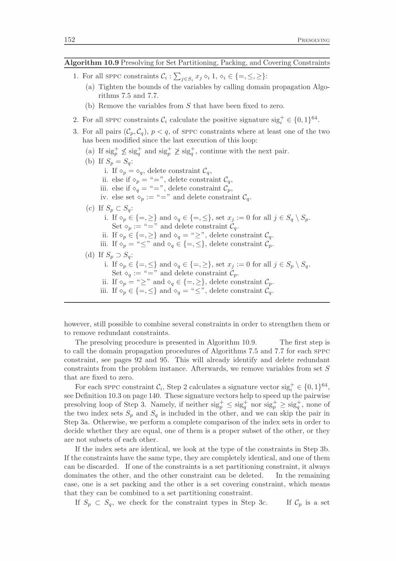
152 Presolving
Algorithm 10.9 Presolving for Set Partitioning, Packing, and Covering Constraints
1. For all sppc constraints Ci :∑
j∈Sixj ⋄i 1, ⋄i ∈ {=,≤,≥}:
(a) Tighten the bounds of the variables by calling domain propagation Algo-rithms 7.5 and 7.7.
(b) Remove the variables from S that have been fixed to zero.
2. For all sppc constraints Ci calculate the positive signature sig+i ∈ {0, 1}
64.
3. For all pairs (Cp, Cq), p < q, of sppc constraints where at least one of the twohas been modified since the last execution of this loop:
(a) If sig+p 6≤ sig+
q and sig+p 6≥ sig+
q , continue with the next pair.
(b) If Sp = Sq:
i. If ⋄p = ⋄q, delete constraint Cq,ii. else if ⋄p = “=”, delete constraint Cq,iii. else if ⋄q = “=”, delete constraint Cp,iv. else set ⋄p := “=” and delete constraint Cq.
(c) If Sp ⊂ Sq:
i. If ⋄p ∈ {=,≥} and ⋄q ∈ {=,≤}, set xj := 0 for all j ∈ Sq \ Sp.Set ⋄p := “=” and delete constraint Cq.
ii. If ⋄p ∈ {=,≥} and ⋄q = “≥”, delete constraint Cq.iii. If ⋄p = “≤” and ⋄q ∈ {=,≤}, delete constraint Cp.
(d) If Sp ⊃ Sq:
i. If ⋄p ∈ {=,≤} and ⋄q ∈ {=,≥}, set xj := 0 for all j ∈ Sp \ Sq.Set ⋄q := “=” and delete constraint Cp.
ii. If ⋄p = “≥” and ⋄q ∈ {=,≥}, delete constraint Cp.iii. If ⋄p ∈ {=,≤} and ⋄q = “≤”, delete constraint Cq.
however, still possible to combine several constraints in order to strengthen them orto remove redundant constraints.
The presolving procedure is presented in Algorithm 10.9. The first step isto call the domain propagation procedures of Algorithms 7.5 and 7.7 for each sppcconstraint, see pages 92 and 95. This will already identify and delete redundantconstraints from the problem instance. Afterwards, we remove variables from set Sthat are fixed to zero.
For each sppc constraint Ci, Step 2 calculates a signature vector sig+i ∈ {0, 1}
64,see Definition 10.3 on page 140. These signature vectors help to speed up the pairwisepresolving loop of Step 3. Namely, if neither sig+
p ≤ sig+q nor sig+
p ≥ sig+q , none of
the two index sets Sp and Sq is included in the other, and we can skip the pair inStep 3a. Otherwise, we perform a complete comparison of the index sets in order todecide whether they are equal, one of them is a proper subset of the other, or theyare not subsets of each other.
If the index sets are identical, we look at the type of the constraints in Step 3b.If the constraints have the same type, they are completely identical, and one of themcan be discarded. If one of the constraints is a set partitioning constraint, it alwaysdominates the other, and the other constraint can be deleted. In the remainingcase, one is a set packing and the other is a set covering constraint, which meansthat they can be combined to a set partitioning constraint.
If Sp ⊂ Sq, we check for the constraint types in Step 3c. If Cp is a set
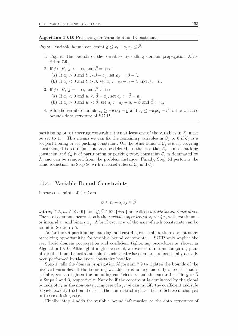
10.4. Variable Bound Constraints 153
Algorithm 10.10 Presolving for Variable Bound Constraints
Input : Variable bound constraint β ≤ xi + ajxj ≤ β.
1. Tighten the bounds of the variables by calling domain propagation Algo-rithm 7.9.
2. If j ∈ B, β > −∞, and β = +∞:
(a) If aj > 0 and li > β − aj , set aj := β − li.
(b) If aj < 0 and li > β, set aj := aj + li − β and β := li.
3. If j ∈ B, β = −∞, and β < +∞:
(a) If aj < 0 and ui < β − aj , set aj := β − ui.
(b) If aj > 0 and ui < β, set aj := aj + ui − β and β := ui.
4. Add the variable bounds xi ≥ −ajxj + β and xi ≤ −ajxj + β to the variablebounds data structure of SCIP.
partitioning or set covering constraint, then at least one of the variables in Sp mustbe set to 1. This means we can fix the remaining variables in Sq to 0 if Cq is aset partitioning or set packing constraint. On the other hand, if Cq is a set coveringconstraint, it is redundant and can be deleted. In the case that Cp is a set packingconstraint and Cq is of partitioning or packing type, constraint Cp is dominated byCq and can be removed from the problem instance. Finally, Step 3d performs thesame reductions as Step 3c with reversed roles of Cp and Cq.
10.4 Variable Bound Constraints
Linear constraints of the form
β ≤ xi + ajxj ≤ β
with xj ∈ Z, aj ∈ R\{0}, and β, β ∈ R∪{±∞} are called variable bound constraints.The most common incarnation is the variable upper bound xi ≤ u
′i xj with continuous
or integral xi and binary xj . A brief overview of the uses of such constraints can befound in Section 7.5.
As for the set partitioning, packing, and covering constraints, there are not manypresolving opportunities for variable bound constraints. SCIP only applies thevery basic domain propagation and coefficient tightening procedures as shown inAlgorithm 10.10. Although it might be useful, we even refrain from comparing pairsof variable bound constraints, since such a pairwise comparison has usually alreadybeen performed by the linear constraint handler.
Step 1 calls the domain propagation Algorithm 7.9 to tighten the bounds of theinvolved variables. If the bounding variable xj is binary and only one of the sidesis finite, we can tighten the bounding coefficient aj and the constraint side β or βin Steps 2 and 3, respectively. Namely, if the constraint is dominated by the globalbounds of xi in the non-restricting case of xj , we can modify the coefficient and sideto yield exactly the bound of xi in the non-restricting case, but to behave unchangedin the restricting case.
Finally, Step 4 adds the variable bound information to the data structures of
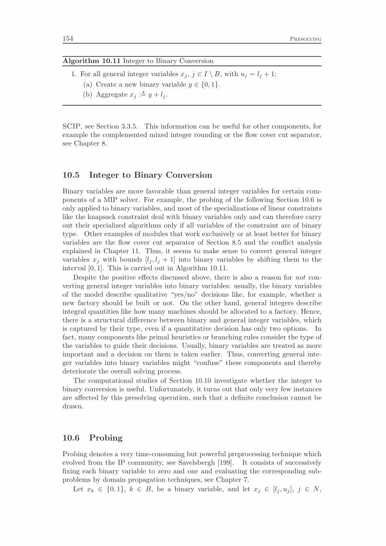
154 Presolving
Algorithm 10.11 Integer to Binary Conversion
1. For all general integer variables xj , j ∈ I \B, with uj = lj + 1:
(a) Create a new binary variable y ∈ {0, 1}.
(b) Aggregate xj : ⋆= y + lj .
SCIP, see Section 3.3.5. This information can be useful for other components, forexample the complemented mixed integer rounding or the flow cover cut separator,see Chapter 8.
10.5 Integer to Binary Conversion
Binary variables are more favorable than general integer variables for certain com-ponents of a MIP solver. For example, the probing of the following Section 10.6 isonly applied to binary variables, and most of the specializations of linear constraintslike the knapsack constraint deal with binary variables only and can therefore carryout their specialized algorithms only if all variables of the constraint are of binarytype. Other examples of modules that work exclusively or at least better for binaryvariables are the flow cover cut separator of Section 8.5 and the conflict analysisexplained in Chapter 11. Thus, it seems to make sense to convert general integervariables xj with bounds [lj , lj + 1] into binary variables by shifting them to theinterval [0, 1]. This is carried out in Algorithm 10.11.
Despite the positive effects discussed above, there is also a reason for not con-verting general integer variables into binary variables: usually, the binary variablesof the model describe qualitative “yes/no” decisions like, for example, whether anew factory should be built or not. On the other hand, general integers describeintegral quantities like how many machines should be allocated to a factory. Hence,there is a structural difference between binary and general integer variables, whichis captured by their type, even if a quantitative decision has only two options. Infact, many components like primal heuristics or branching rules consider the type ofthe variables to guide their decisions. Usually, binary variables are treated as moreimportant and a decision on them is taken earlier. Thus, converting general inte-ger variables into binary variables might “confuse” these components and therebydeteriorate the overall solving process.
The computational studies of Section 10.10 investigate whether the integer tobinary conversion is useful. Unfortunately, it turns out that only very few instancesare affected by this presolving operation, such that a definite conclusion cannot bedrawn.
10.6 Probing
Probing denotes a very time-consuming but powerful preprocessing technique whichevolved from the IP community, see Savelsbergh [199]. It consists of successivelyfixing each binary variable to zero and one and evaluating the corresponding sub-problems by domain propagation techniques, see Chapter 7.
Let xk ∈ {0, 1}, k ∈ B, be a binary variable, and let xj ∈ [lj , uj ], j ∈ N ,
10.6. Probing 155
denote some other (binary or non-binary) variable. Let l0j and u0j be the lower and
upper bounds of xj that have been deduced from xk = 0. Let l1j and u1j be the
corresponding bounds of xj deduced from xk = 1. The following observations canbe made:
⊲ If one of the fixings of xk leads to an infeasible subproblem, xk can be per-manently fixed to the opposite value and removed from the problem instance.
⊲ If l0j = u0j and l1j = u1
j , xj can be aggregated as xj : ⋆= l0j + (l1j − l0j )xk.
⊲ l′j := min{l0j , l1j } and u′j := max{u0
j , u1j} are valid global bounds of xj .
⊲ xk = 0 → l0j ≤ xj ≤ u0j and xk = 1 → l1j ≤ xj ≤ u1
j are valid implicationsthat can be stored in the implication graph of SCIP, see Section 3.3.5, andexploited during the solving process, e.g., in other preprocessing algorithms orin the branching variable selection.
The problematic issue with probing is its runtime complexity. In its full version,we have to execute the complete domain propagation loop twice for each binaryvariable. In order to avoid spending too much time on probing, one usually employsonly a limited version of probing. One possible limitation is to restrict the number ofrounds in each domain propagation loop. This can be done in SCIP via a parametersetting, but the default value of this parameter is to execute the domain propagationloop with an unlimited number of rounds, i.e., until no more deductions have beenfound.
Another possibility to speed up the algorithm is to not apply probing to all binaryvariables, but only to a subset of promising candidates. This approach is used inSCIP. The binary variables are sorted such that the most promising candidatesare evaluated first. If the probing does not produce any useful information forsome number of consecutive evaluated candidates, the probing algorithm is aborted.Additionally, we interrupt the probing loop after fixings or aggregations have beenfound in order to apply the other, less expensive presolving methods. The hope isthat they are able to further reduce the size of the problem instance and to increasethe chances for probing to find additional reductions. Afterwards, probing continueswith the next candidate in its sorted list of binary variables.
Algorithm 10.12 depicts the details of the probing procedure. Note with defaultsettings, probing is called in a “delayed” fashion, which means that it is skipped aslong as other presolving components found reductions that trigger another round ofpresolving.
Step 1 of the algorithm checks whether the probing loop was aborted due toexcessive useless probings, compare Step 4f. If this is the case, and no relevantchanges have been applied to the instance by other presolving methods since the lastprobing call, we exit again. Otherwise, we reduce the “useless” counters by 10 % inStep 2 to allow for some more probings, even if the probing loop was aborted duringthe last call due to too many successive useless probings.
If the binary variables have not already been sorted, this is performed in Step 3.The score sj of a variable xj estimates the impact of fixing xj to 0 or 1. It considersthe following statistics:
⊲ the number of constraints ζ−j and ζ+j that get “less feasible” by setting xj to
0 and 1, respectively (in a MIP, the sum ζ−j + ζ+j is equal to the total number

156 Presolving
Algorithm 10.12 Probing
Input : Current values of counters startidx, nuseless, and ntotaluseless.
1. If probing was aborted in the last call, no variables have been fixed or aggre-gated, and no domains have been tightened since the last call, abort.
2. Set nuseless := 0.9 · nuseless and ntotaluseless := 0.9 · ntotaluseless.
3. If not already performed, generate a sorted list S = {k1, . . . , kq} of the binaryvariables xki
, ki ∈ B: sort variables by non-increasing score
sj = ζ−j + ζ+j +
∣∣δ−D(xj = 0)
∣∣+∣∣δ−D(xj = 1)
∣∣+ 5
∣∣Q(xj = 0)
∣∣+ 5
∣∣Q(xj = 1)
∣∣.
with D = (V,A) being the implication graph and Q being the clique table.
4. For i = startidx, . . . , q:
(a) If xkihas been fixed or aggregated, continue Loop 4 with the next can-
didate.
(b) For v = 0, 1:
i. Tentatively fix xki:= v.
ii. Propagate implications δ−D(xki= v) and cliques Q(xki
= v) to obtain
implied bounds [lv, uv ] ⊆ [l, u].
iii. Call domain propagation to obtain implied bounds [lv, uv] ⊆ [lv, uv].iv. Reset lki
:= 0, uki:= 1, and undo all implied bound changes.
(c) If propagation of xki= 0 deduced a conflict, fix xki
:= 1.If propagation of xki
= 1 deduced a conflict, fix xki:= 0.
(d) For all j = 1, . . . , n, j 6= ki:
i. Set lj := min{l0j , l1j } and uj := max{u0
j , u1j}.
ii. If l0j = u0j and l1j = u1
j , aggregate xj : ⋆= l0j + (l1j − l0j )xki
.
iii. If l0j > lj , add xki= 0→ xj ≥ l
0j to the implication graph.
If u0j < uj , add xki
= 0→ xj ≤ u0j to the implication graph.
If l1j > lj , add xki= 1→ xj ≥ l
1j to the implication graph.
If u1j < uj , add xki
= 1→ xj ≤ u1j to the implication graph.
(e) Increase nuseless and ntotaluseless. If a variable has been fixed or aggre-gated in Loop 4d, reset nuseless := 0 and ntotaluseless := 0. If a boundhas been tightened in Loop 4d, reset ntotaluseless := 0.
(f) If nuseless ≥ 2000 or ntotaluseless ≥ 100, abort Loop 4.
(g) If at least 50 variables have been fixed or aggregated in this probing call,interrupt Loop 4.
5. Set startidx := i+ 1.
10.7. Implication Graph Analysis 157
of constraints the variable is contained in, counting equations and ranged rowstwice), see Definition 3.3 on page 38,
⊲ the number of implications that are triggered by xj = 0 and xj = 1, and
⊲ the number of cliques |Q(xj = v)| the variable is contained in as negative(v = 0) or positive (v = 1) literal, see Section 3.3.5.
We count each clique as 5 implications, which means we estimate the average cliquesize to be 6.
Step 4 represents the main probing loop in which the probing is applied to theindividual candidates xki
of the sorted candidate list S. At first, we check in Step 4awhether the candidate is still an active variable. If it has been fixed or aggregatedsince the candidate list was generated, we skip the candidate. Step 4b performsthe actual work of propagating the settings xki
= 0 and xki= 1. Note that we
first propagate the known implications in the implication graph and clique table inorder to be able to identify unknown implications in the evaluation of Step 4(d)iii.Otherwise, we would generate the same implications over and over again and wastea considerable amount of time in the implication graph management. After havingperformed the implication and clique propagation we propagate the constraints.
Steps 4c and 4d evaluate the results of the probing. If one of the tentativefixings lead to an infeasibility, the probing variable can be fixed to the other valuein Step 4c. If both probing directions produced a conflict, we conclude that theinstance is infeasible and can abort the solving process. Note that if xki
has beenfixed to xki
:= v, we can immediately tighten the bounds of the other variablesto l := lv and u := uv. Otherwise, we inspect the bound deductions in Loop 4d.First, we can tighten the bounds of each variable xj as indicated in Step 4(d)i. Ifthis leads to a fixed variable lj = uj , we can skip the remaining steps and continueLoop 4d with the next variable. If the variable xj is forced to one of its bounds inboth probing directions, we can aggregate it in Step 4(d)ii. Otherwise, we compare
the deduced bounds [lvj , uvj ] with the known implied bounds [lvj , u
vj ] in Step 4(d)iii
and add previously unknown implications to the implication graph of SCIP.Step 4e updates the nuseless and ntotaluseless counters. We call a probing useless
if it did not produce any fixings or aggregations of variables. If it even did not help totighten a bound of a variable, we call it totally useless. We abort the probing loop inStep 4f if 2000 successive useless probings or 100 successive totally useless probingshave been conducted. As mentioned above, we interrupt the probing process inStep 4g if it seems beneficial to further reduce the problem instance by applyingother, less expensive presolving techniques. In the default settings of SCIP, probingis interrupted after a total number of 50 fixings or aggregations have been found inLoop 4. Finally, in Step 5 we record the index of the candidate with which we wantto continue the probing loop in the next execution of the algorithm.
10.7 Implication Graph Analysis
As mentioned in the previous section, probing is a very time-consuming presolvingtechnique and is therefore delayed until all other presolving components failed to findmore reductions. Additionally, probing may be aborted prematurely. However, onepart of probing can be implemented much more efficiently, namely the extraction offixings and aggregations out of the implication graph. Therefore, this part of probingis replicated in an additional presolving plugin: the implication graph analysis.
158 Presolving
Algorithm 10.13 Implication Graph Analysis
1. For all binary variables xk, k ∈ B, and all variables xj , j ∈ N , that are impliedvariables in both implication lists, δ−D(xk = 0) and δ−D(xk = 1):
(a) If xk = 0→ xj ≥ l0j and xk = 1→ xj ≥ l
1j , tighten lj := min{l0j , l
1j }.
(b) If xk = 0→ xj ≤ u0j and xk = 1→ xj ≤ u
1j , tighten uj := max{u0
j , u1j}.
(c) If xk = 0→ xj ≤ lj and xk = 1→ xj ≥ uj , aggr. xj : ⋆= lj + (uj − lj)xk.
(d) If xk = 0→ xj ≥ uj and xk = 1→ xj ≤ lj , aggr. xj : ⋆= uj − (uj − lj)xk.
The idea is to compare for each binary variable xk, k ∈ B, the list of implicationsδ−D(xk = 0) and δ−D(xk = 1). Since these lists are sorted by the index of the impliedvariable, they can be scanned in linear time w.r.t. the sum of their lengths in orderto identify variables xj that appear in both lists. The following conclusions can bemade, which are similar to Steps 4(d)i and 4(d)ii of the probing Algorithm 10.12:
xk = 0→ xj ≥ l0j ∧ xk = 1→ xj ≥ l
1j ⇒ xj ≥ min{l0j , l
1j}
xk = 0→ xj ≤ u0j ∧ xk = 1→ xj ≤ u
1j ⇒ xj ≤ max{u0
j , u1j}
xk = 0→ xj = lj ∧ xk = 1→ xj = uj ⇒ xj⋆= lj + (uj − lj)xk
xk = 0→ xj = uj ∧ xk = 1→ xj = lj ⇒ xj⋆= uj − (uj − lj)xk
The procedure is summarized in Algorithm 10.13. Note that the implicationgraph stores only non-redundant implications. This means the implied bounds arealways tighter than the global bounds, and we do not have to check whether theminimum or maximum of the implied bounds used in Steps 1a and 1b is indeedbetter than the current global bound lj or uj , respectively.
10.8 Dual Fixing
Despite a few steps in the linear constraint presolving, all presolving techniquespresented so far are so-called primal presolving algorithms. They are purely based onfeasibility arguments and are therefore valid independently of the objective function.
In contrast, the reasoning of dual presolving techniques is based on optimalityconsiderations. For example, if we can prove that for every optimal solution x⋆
there exists a solution x with the same objective value c⋆ = cTx⋆ = cT x in whicha certain variable xj has a specific value xj = v, we can fix xj := v. Thereby, wemay rule out a number of feasible solutions, but we are still sure that the feasibilitystatus of the instance does not change and that an optimal solution for the presolvedinstance is also optimal in the original instance.
Dual presolving can be interpreted as primal presolving in the dual space. Forexample, like for primal variables, bound tightening can also be applied in the dualspace for the dual variables and the reduced costs. If we find out that a dualvariable yi of a linear constraint Ci : aTx ≤ β is always negative, we can conclude bythe complementary slackness that the corresponding primal slack variable is alwayszero and the inequality is always satisfied with equality, i.e., aTx = β. As anadditional example, if we can prove that a reduced cost rj is always positive, wecan again by the complementary slackness conclude that the primal variable xj willalways be at its lower bound, and we can fix xj := lj . Other dual reductions exploit
10.8. Dual Fixing 159
Algorithm 10.14 Dual Fixing
1. For all variables xj , j ∈ N :
(a) If cj ≥ 0 and ζ−j = 0, fix xj := lj .
(b) If cj ≤ 0 and ζ+j = 0, fix xj := uj .
(c) If the variable xj has been fixed to an infinite value and cj 6= 0, concludethat the instance is either unbounded or infeasible.
column domination (which is the dual analogon of constraint domination, compareStep 2d of the pairwise linear constraint presolving Algorithm 10.5 on page 141) andsymmetric sets of variables.
The common property of dual presolving algorithms is that they look at thecolumns A·j of the coefficient matrix of the MIP. Unfortunately, the constraintbased approach of SCIP does not support such a dual view of the problem instance,since the constraint data are stored in private data structures of the constraint han-dlers. This means, the necessary problem information is not accessible via frameworkmethods, and even each constraint handler has only partial information about theproblem.
A small step to remedy this situation is that SCIP explicitly collects a limitedamount of dual information, which has to be provided by the constraint handlers, seeSection 3.3.3. This information exists in the form of variable locks, see Definition 3.3on page 38. For a MIP with inequality system Ax ≤ b, the down-locks ζ−j count
the number of negative entries in the column A·j , while the up-locks ζ+j are the
number of positive entries in A·j . More generally, for a constraint integer programthe variable locks ζ−j and ζ+
j count the number of constraints that get “less feasible”by decreasing or increasing the value of xj , respectively.
Having this information at hand, we can perform the so-called dual fixing, whichmeans to fix a variable to its lower or upper bound whenever this is neither harm-ful to the objective function value nor to the feasibility of the constraints. Thisstraightforward procedure is depicted in Algorithm 10.14.
For each variable xj , Step 1a checks whether we can safely fix the variable toits lower bound without increasing the objective function value or increasing theviolation of a constraint. Step 1b applies the same reasoning for the upper bound.It may happen that the variable gets fixed to an “infinite” value, since the boundsdo not need to be finite. From a practical point of view, this is not a big issue: wejust fix the variable to a very large value which is considered as infinity. Then, allconstraints will be deleted as redundant that contain this variable. If the objectivecoefficient cj of such a variable is non-zero, however, we end up with an infiniteobjective function value. This means, the instance is either unbounded or infeasible,depending on whether there is a feasible solution for the remaining constraints andvariables. As other MIP solvers like Cplex [118] or Xpress [76], SCIP terminatesin this situation with the undecided status “infeasible or unbounded”. In orderto decide the feasibility status of the instance, one can solve the model withoutobjective function by setting c := 0.
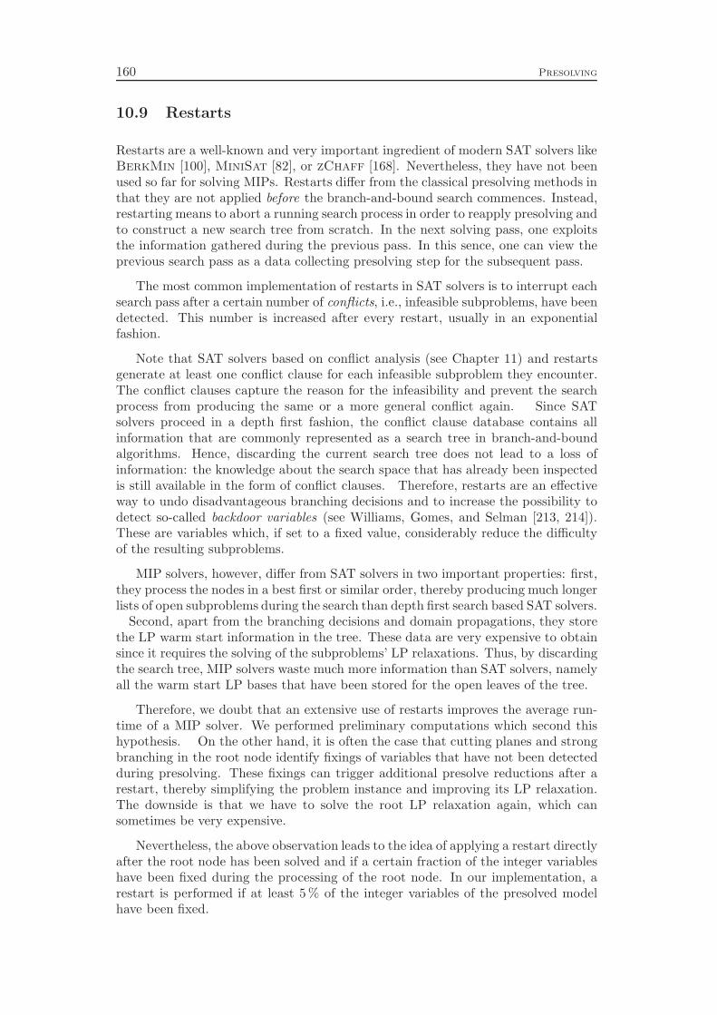
160 Presolving
10.9 Restarts
Restarts are a well-known and very important ingredient of modern SAT solvers likeBerkMin [100], MiniSat [82], or zChaff [168]. Nevertheless, they have not beenused so far for solving MIPs. Restarts differ from the classical presolving methods inthat they are not applied before the branch-and-bound search commences. Instead,restarting means to abort a running search process in order to reapply presolving andto construct a new search tree from scratch. In the next solving pass, one exploitsthe information gathered during the previous pass. In this sence, one can view theprevious search pass as a data collecting presolving step for the subsequent pass.
The most common implementation of restarts in SAT solvers is to interrupt eachsearch pass after a certain number of conflicts, i.e., infeasible subproblems, have beendetected. This number is increased after every restart, usually in an exponentialfashion.
Note that SAT solvers based on conflict analysis (see Chapter 11) and restartsgenerate at least one conflict clause for each infeasible subproblem they encounter.The conflict clauses capture the reason for the infeasibility and prevent the searchprocess from producing the same or a more general conflict again. Since SATsolvers proceed in a depth first fashion, the conflict clause database contains allinformation that are commonly represented as a search tree in branch-and-boundalgorithms. Hence, discarding the current search tree does not lead to a loss ofinformation: the knowledge about the search space that has already been inspectedis still available in the form of conflict clauses. Therefore, restarts are an effectiveway to undo disadvantageous branching decisions and to increase the possibility todetect so-called backdoor variables (see Williams, Gomes, and Selman [213, 214]).These are variables which, if set to a fixed value, considerably reduce the difficultyof the resulting subproblems.
MIP solvers, however, differ from SAT solvers in two important properties: first,they process the nodes in a best first or similar order, thereby producing much longerlists of open subproblems during the search than depth first search based SAT solvers.
Second, apart from the branching decisions and domain propagations, they storethe LP warm start information in the tree. These data are very expensive to obtainsince it requires the solving of the subproblems’ LP relaxations. Thus, by discardingthe search tree, MIP solvers waste much more information than SAT solvers, namelyall the warm start LP bases that have been stored for the open leaves of the tree.
Therefore, we doubt that an extensive use of restarts improves the average run-time of a MIP solver. We performed preliminary computations which second thishypothesis. On the other hand, it is often the case that cutting planes and strongbranching in the root node identify fixings of variables that have not been detectedduring presolving. These fixings can trigger additional presolve reductions after arestart, thereby simplifying the problem instance and improving its LP relaxation.The downside is that we have to solve the root LP relaxation again, which cansometimes be very expensive.
Nevertheless, the above observation leads to the idea of applying a restart directlyafter the root node has been solved and if a certain fraction of the integer variableshave been fixed during the processing of the root node. In our implementation, arestart is performed if at least 5 % of the integer variables of the presolved modelhave been fixed.
10.10. Computational Results 161
test set none no linear pairs aggreg linear pairs no knap disaggregti
me
miplib +65 −2 +2 −1
coral +93 −3 −5 +10
milp +82 +4 +10 +8
enlight −7 −1 −2 −2
alu +248 −6 −10 −1
fctp +130 +3 +2 0
acc +112 +7 +16 +19
fc +372 +1 +1 0
arcset +72 +24 −1 +2
mik +458 +9 +2 −1
total +91 +1 +2 +5
no
des
miplib +163 +2 −2 +3
coral +126 −4 −6 +11
milp +128 +10 +14 +1
enlight +50 0 0 0
alu +398 −23 −43 0
fctp +402 0 0 0
acc +233 +35 +33 +62
fc +2589 −8 −4 0
arcset +114 +60 +8 0
mik +204 −1 0 0
total +162 +3 +1 +6
Table 10.1. Performance effect of various presolving methods for solving MIP instances. Thevalues denote the percental changes in the shifted geometric mean of the runtime (top) and num-ber of branching nodes (bottom) compared to the default settings. Positive values represent adeterioration, negative values an improvement.
10.10 Computational Results
In this section we present benchmarks that evaluate various aspects of MIP presolv-ing. Table 10.1 and 10.2 show the effect of disabling particular presolving methods.Detailed results can be found in Tables B.161 to B.180.
Column “none” of Table 10.1 yields the results for disabling presolving com-pletely. Apart from the enlight instances, presolving significantly improves theperformance on all test sets. Overall, disabling presolving almost leads to a dou-bling of the runtime and to an even larger increase in the number of branching nodesthat have to be processed.
The remaining columns of Table 10.1 deal with certain subroutines in the linearand knapsack presolving. Disabling the presolving of pairs of linear constraints asdepicted in Algorithm 10.5 yields the average performance ratios shown in column“no linear pairs”. Besides the arcset, mik, and acc test sets, the impact of thismethod is rather weak.
The constraint aggregation Steps 2f and 2g of Algorithm 10.5 are disabled inthe default settings. This decreases the runtime overhead of the pairwise presolvingalgorithm, since we can also rule out constraint pairs by the signature check inStep 2a that include equations. Activating this rather expensive step yields theresults shown in column “aggreg linear pairs”. The constraint aggregation can onlyimprove the performance on the coral and alu instances by a significant amount,even if we consider the number of nodes instead of the runtime. Overall, it leads toa slight deterioration.
The column labeled “no knap disaggreg” shows the benchmarks for disabling theknapsack clique disaggregation. This means, the coefficient tightening Step 7 of theknapsack presolving Algorithm 10.8 is skipped. Although it has been argued byother researchers, for example Bixby et al. [46] and Fügenschuh and Martin [90],
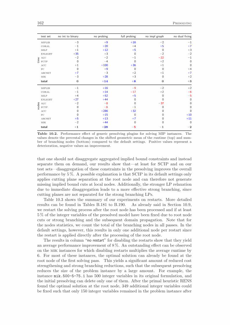
162 Presolving
test set no int to binary no probing full probing no impl graph no dual fixingti
me
miplib −3 +9 +16 −2 −1
coral −1 +20 +4 +5 +7
milp +1 +12 +5 0 +3
enlight +35 +3 0 −2 −2
alu −2 −2 −1 −22 −1
fctp 0 −4 0 +2 0
acc +1 +100 +36 +1 0
fc 0 +9 0 0 +4
arcset +7 −3 +2 +1 +7
mik −3 +28 +3 0 +2
total 0 +14 +8 0 +3
no
des
miplib −1 +16 −9 −2 +2
coral −1 +14 −17 +2 −6
milp +4 +52 +5 0 −5
enlight +27 +44 0 0 0
alu −2 −8 0 −37 0
fctp 0 −6 −1 0 0
acc 0 +286 +32 0 0
fc 0 +15 0 0 +10
arcset +5 +13 +7 0 +11
mik −2 +44 0 0 0
total +1 +28 −5 −1 −2
Table 10.2. Performance effect of generic presolving plugins for solving MIP instances. Thevalues denote the percental changes in the shifted geometric mean of the runtime (top) and num-ber of branching nodes (bottom) compared to the default settings. Positive values represent adeterioration, negative values an improvement.
that one should not disaggregate aggregated implied bound constraints and insteadseparate them on demand, our results show that—at least for SCIP and on ourtest sets—disaggregation of these constraints in the presolving improves the overallperformance by 5 %. A possible explanation is that SCIP in its default settings onlyapplies cutting plane separation at the root node and can therefore not generatemissing implied bound cuts at local nodes. Additionally, the stronger LP relaxationdue to immediate disaggregation leads to a more effective strong branching, sincecutting planes are not separated for the strong branching LPs.
Table 10.3 shows the summary of our experiments on restarts. More detailedresults can be found in Tables B.181 to B.190. As already said in Section 10.9,we restart the solving process after the root node has been processed and if at least5 % of the integer variables of the presolved model have been fixed due to root nodecuts or strong branching and the subsequent domain propagation. Note that forthe nodes statistics, we count the total of the branching nodes in all passes. In thedefault settings, however, this results in only one additional node per restart sincethe restart is applied directly after the processing of the root node.
The results in column “no restart” for disabling the restarts show that they yieldan average performance improvement of 8 %. An outstanding effect can be observedon the mik instances for which disabling restarts multiplies the average runtime by6. For most of these instances, the optimal solution can already be found at theroot node of the first solving pass. This yields a significant amount of reduced coststrengthening and strong branching reductions, such that the subsequent presolvingreduces the size of the problem instance by a large amount. For example, theinstance mik.500-5-75.1 has 500 integer variables in its original formulation, andthe initial presolving can delete only one of them. After the primal heuristic RENSfound the optimal solution at the root node, 349 additional integer variables couldbe fixed such that only 150 integer variables remained in the problem instance after

10.10. Computational Results 163
test set no restart sub restart aggr sub restartti
me
miplib +3 +2 +4
coral −1 0 +2
milp +10 +12 +14
enlight −1 −1 −1
alu 0 +1 0
fctp +3 +2 +1
acc +3 −1 +1
fc +1 +1 +2
arcset +9 −1 +1
mik +500 0 +1
total +8 +4 +6
no
des
miplib −4 +3 +2
coral −4 +3 +2
milp +19 +15 +21
enlight 0 0 0
alu 0 0 −13
fctp 0 0 0
acc 0 0 0
fc +8 −2 −8
arcset +4 −6 −3
mik +310 0 0
total +7 +6 +6
Table 10.3. Performance effect of using restarts for solving MIP instances. The values denotethe percental changes in the shifted geometric mean of the runtime (top) and number of branchingnodes (bottom) compared to the default settings. Positive values represent a deterioration, negativevalues an improvement.
the restart. Additionally, the second presolving reduced the number of rows in theLP from 324 to 249, although the dual bound at the root node improved.
We also experimented with applying a restart during the branch-and-boundsearch after a certain fraction of the integer variables has been globally fixed.Such global fixings can be identified, for example, by the root reduced cost streng-thening, see Section 7.7, or if one of the two subtrees of the root node has beenprocessed completely and has therefore been cut off from the tree.
Unfortunately, the results are inferior to the default settings. Column “sub restart”gives the results for applying an additional restart each time when the number ofglobally fixed integer variables exceeded 10 % of the total number of integer vari-ables in the presolved model. The settings used to produce the results of column“aggr sub restart” are even more aggressive: here, the solving process is alreadyrestarted if 5 % of the integer variables have been globally fixed. A cursory inspec-tion of the log files indicates that global variable fixings happen very infrequentlyduring the processing of the subproblems, and if a significant amount of additionalvariables has been globally fixed, the search is usually almost finished such that arestart at this point is very disadvantegeous. Therefore, in order to make good useof delayed restarts, one has to invent different criteria for their application.

Chapter 11
Conflict Analysis
The branch-and-bound algorithm to solve mixed integer programs divides the givenproblem instance into smaller subproblems and iterates this process recursively untilan optimal solution of the respective subproblem can be identified or the subproblemis detected to be infeasible or to exceed the primal bound. It seems that currentstate-of-the-art MIP solvers like Cplex [118], Lingo [148], SIP [159], or Xpress [76]simply discard infeasible and bound-exceeding subproblems without paying furtherattention to them.
The satisfiability problem can also be solved by a branch-and-bound decompo-sition scheme, which was originally proposed in this context by Davis, Putnam,Logemann, and Loveland [77, 78], hence the name DPLL algorithm. In contrast toMIP solvers, modern SAT solvers try to learn from infeasible subproblems, whichis an idea due to Marques-Silva and Sakallah [157]. The infeasibilities are ana-lyzed in order to generate so-called conflict clauses. These are implied clauses thathelp to prune the search tree. They also enable the solver to apply so-called non-chronological backtracking.
The idea of conflict analysis is to identify a reason for the infeasibility of thecurrent subproblem and to exploit this knowledge later in the search. In SAT solving,such a reason is a subset of the current variable fixings that already suffices to triggera chain of logical deductions that ends in a contradiction. This means, the fixing ofthe variables of this conflict set renders the problem instance infeasible. The conflictclause that can be learned from this conflict states that at least one of the variablesin the conflict set has to take the opposite truth value. This clause is added tothe clause database and can then be used at other subproblems to find additionalimplications in domain propagation, thereby pruning the search tree.
A similar idea of conflict analysis are the so-called no-goods, which emergedfrom the constraint programming community, see, e.g., Stallman and Sussman [201],Ginsberg [94], and Jiang, Richards, and Richards [124]. They can be seen as ageneralization of conflict clauses to the domain of constraint programming.
In this chapter, we describe a generalization of conflict analysis to branch-and-bound based mixed integer programming and constraint integer programming. Thesame generalization was independently developed by Sandholm and Shields [198].Parts of this chapter have been published in Achterberg [1].
Suppose a subproblem in the branch-and-bound search tree is detected to beinfeasible or to exceed the primal bound. We will show that this situation can beanalyzed with similar techniques as in SAT solving: a conflict graph is constructedfrom which conflict constraints can be extracted. These constraints can be usedas cutting planes and in domain propagation to strengthen the relaxations of othersubproblems in the tree.
Note that the term “conflict graph” is used differently in the SAT and MIPcommunities. In MIP solving, the conflict graph consists of implications betweentwo binary variables each, see e.g., Atamtürk, Nemhauser, and Savelsbergh [24]. Itrepresents a vertex-packing relaxation of the MIP instance and can, for instance,
165
166 Conflict Analysis
be used to derive cutting planes like clique cuts, see Section 8.7. In SAT solving,and also in this chapter, the conflict graph represents the deductions that have beenperformed in order to prove the infeasibility of the current subproblem.
There are two main differences of MIP and SAT solving in the context of conflictanalysis. First, the variables of an MIP need not to be of binary type; we alsohave to deal with general integer and continuous variables. Furthermore, theinfeasibility of a subproblem in the MIP search tree usually has its sources in thelinear programming (LP) relaxation of the subproblem. In this case, we first haveto find a (preferably simple) reason for the LP’s infeasibility before we can applythe SAT conflict analysis techniques for generating conflict constraints.
This chapter is organized as follows. Section 11.1 reviews conflict graph analysisof SAT solvers. For an infeasible subproblem, it is shown how to generate the conflictgraph and how to extract valid conflict clauses out of this graph. Section 11.2deals with the generalization of these techniques to mixed integer programming.We explain how infeasible and bound-exceeding linear programs can be analyzed inorder to detect a conflict in the local bounds of the variables. This conflict is usedas starting point to construct the conflict graph from which conflict constraints canbe extracted with the techniques explained in Section 11.1. Additionally, we discusshow we generalize the notion of the conflict graph in the presence of non-binaryvariables. Experimental results in Section 11.3 demonstrate that conflict analysisleads to savings in the average number of branching nodes and the average timeneeded to solve MIPs. As the results of Chapter 17 show, conflict analysis is a keyingredient for solving the chip design verification problem with our constraint integerprogramming approach.
11.1 Conflict Analysis in SAT Solving
In this section we review the conflict analysis techniques used in SAT solving, seee.g., Marques-Silva and Sakallah [157] or Zhang et al. [224]. We recapitulate thedefinition of the satisfiability problem (SAT), see Section 1.2.
Definition (satisfiability problem). Let C = C1 ∧ . . . ∧ Cm be a logic formulain conjunctive normal form (CNF) on Boolean variables x1, . . . , xn. Each clauseCi = ℓi1∨. . .∨ℓ
iki
is a disjunction of literals. A literal ℓ ∈ L = {x1, . . . , xn, x1, . . . , xn}is either a variable xj or the negation of a variable xj . The task of the satisfiabilityproblem (SAT) is to either find an assignment x⋆ ∈ {0, 1}n, such that the formula C
is satisfied, i.e., each clause Ci evaluates to 1, or to conclude that C is unsatisfiable,i.e., for all x ∈ {0, 1}n at least one Ci evaluates to 0.
The DPLL-algorithm to solve SAT problems fixes one of the binary variables to0 or 1 at each node in the search tree. Then, Boolean constraint propagation (BCP)deduces further fixings by applying the domain propagation rule
∀j ∈ {1, . . . , ki} \ {p} : ℓij = 0 → ℓip = 1
on the clauses Ci = ℓi1 ∨ . . . ∨ ℓiki
, i = 1, . . . ,m, compare the domain propagation ofset covering constraints in Section 7.4. This rule is triggered if the deletion of falseliterals reduces a still unsatisfied clause to a single literal, a so-called unit clause. Inthis case, the remaining literal can be fixed to 1. BCP is applied iteratively until no
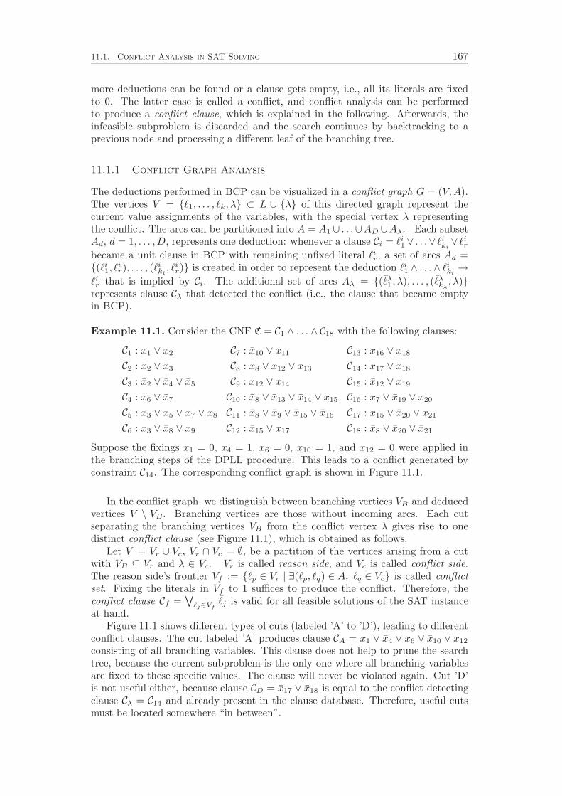
11.1. Conflict Analysis in SAT Solving 167
more deductions can be found or a clause gets empty, i.e., all its literals are fixedto 0. The latter case is called a conflict, and conflict analysis can be performedto produce a conflict clause, which is explained in the following. Afterwards, theinfeasible subproblem is discarded and the search continues by backtracking to aprevious node and processing a different leaf of the branching tree.
11.1.1 Conflict Graph Analysis
The deductions performed in BCP can be visualized in a conflict graph G = (V,A).The vertices V = {ℓ1, . . . , ℓk, λ} ⊂ L ∪ {λ} of this directed graph represent thecurrent value assignments of the variables, with the special vertex λ representingthe conflict. The arcs can be partitioned into A = A1 ∪ . . .∪AD ∪Aλ. Each subsetAd, d = 1, . . . ,D, represents one deduction: whenever a clause Ci = ℓi1∨ . . .∨ ℓ
iki∨ ℓir
became a unit clause in BCP with remaining unfixed literal ℓir, a set of arcs Ad ={(ℓi1, ℓ
ir), . . . , (ℓ
iki, ℓir)} is created in order to represent the deduction ℓi1 ∧ . . . ∧ ℓ
iki→
ℓir that is implied by Ci. The additional set of arcs Aλ = {(ℓλ1 , λ), . . . , (ℓλkλ, λ)}
represents clause Cλ that detected the conflict (i.e., the clause that became emptyin BCP).
Example 11.1. Consider the CNF C = C1 ∧ . . . ∧ C18 with the following clauses:
C1 : x1 ∨ x2 C7 : x10 ∨ x11 C13 : x16 ∨ x18
C2 : x2 ∨ x3 C8 : x8 ∨ x12 ∨ x13 C14 : x17 ∨ x18
C3 : x2 ∨ x4 ∨ x5 C9 : x12 ∨ x14 C15 : x12 ∨ x19
C4 : x6 ∨ x7 C10 : x8 ∨ x13 ∨ x14 ∨ x15 C16 : x7 ∨ x19 ∨ x20
C5 : x3 ∨ x5 ∨ x7 ∨ x8 C11 : x8 ∨ x9 ∨ x15 ∨ x16 C17 : x15 ∨ x20 ∨ x21
C6 : x3 ∨ x8 ∨ x9 C12 : x15 ∨ x17 C18 : x8 ∨ x20 ∨ x21
Suppose the fixings x1 = 0, x4 = 1, x6 = 0, x10 = 1, and x12 = 0 were applied inthe branching steps of the DPLL procedure. This leads to a conflict generated byconstraint C14. The corresponding conflict graph is shown in Figure 11.1.
In the conflict graph, we distinguish between branching vertices VB and deducedvertices V \ VB . Branching vertices are those without incoming arcs. Each cutseparating the branching vertices VB from the conflict vertex λ gives rise to onedistinct conflict clause (see Figure 11.1), which is obtained as follows.
Let V = Vr ∪ Vc, Vr ∩ Vc = ∅, be a partition of the vertices arising from a cutwith VB ⊆ Vr and λ ∈ Vc. Vr is called reason side, and Vc is called conflict side.The reason side’s frontier Vf := {ℓp ∈ Vr | ∃(ℓp, ℓq) ∈ A, ℓq ∈ Vc} is called conflictset. Fixing the literals in Vf to 1 suffices to produce the conflict. Therefore, theconflict clause Cf =
∨
ℓj∈Vfℓj is valid for all feasible solutions of the SAT instance
at hand.Figure 11.1 shows different types of cuts (labeled ’A’ to ’D’), leading to different
conflict clauses. The cut labeled ’A’ produces clause CA = x1 ∨ x4 ∨ x6 ∨ x10 ∨ x12
consisting of all branching variables. This clause does not help to prune the searchtree, because the current subproblem is the only one where all branching variablesare fixed to these specific values. The clause will never be violated again. Cut ’D’is not useful either, because clause CD = x17 ∨ x18 is equal to the conflict-detectingclause Cλ = C14 and already present in the clause database. Therefore, useful cutsmust be located somewhere “in between”.
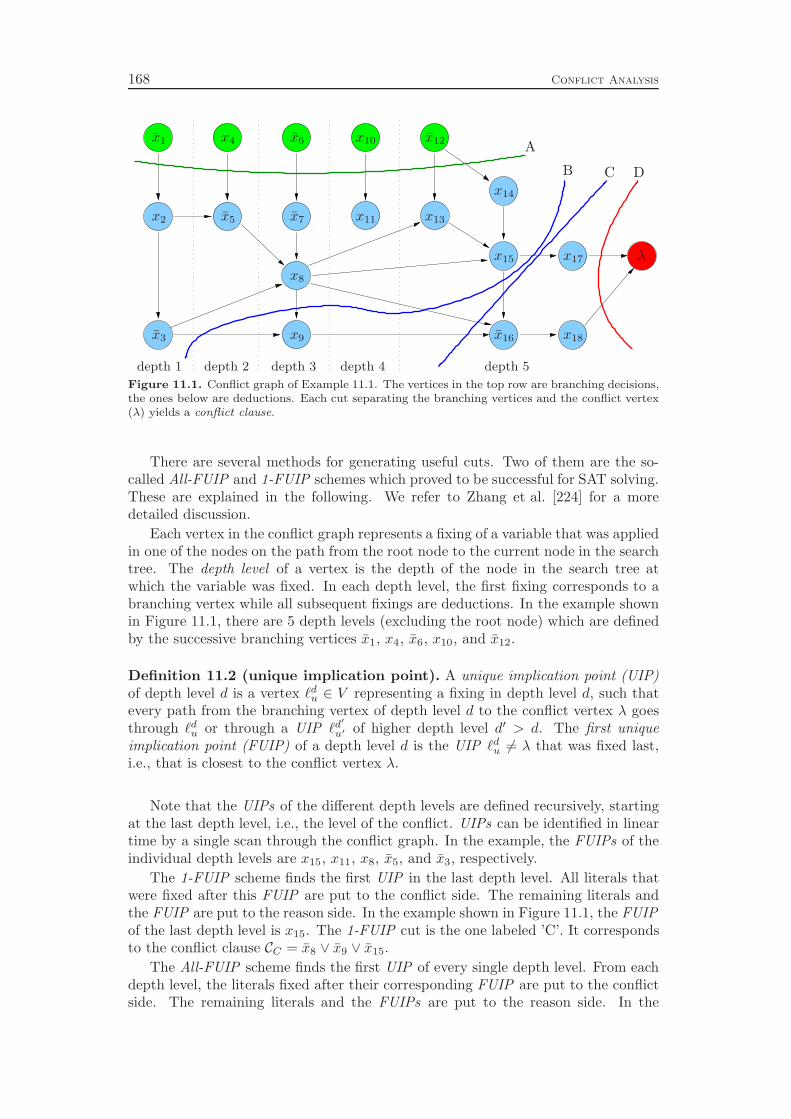
168 Conflict Analysis
x1
x2
x3
x4
x5
x6
x7
x8
x9
x10
x11
x12
x13
x14
x15
x16
x17
x18
λ
A
B C D
depth 1 depth 2 depth 3 depth 4 depth 5
Figure 11.1. Conflict graph of Example 11.1. The vertices in the top row are branching decisions,the ones below are deductions. Each cut separating the branching vertices and the conflict vertex(λ) yields a conflict clause.
There are several methods for generating useful cuts. Two of them are the so-called All-FUIP and 1-FUIP schemes which proved to be successful for SAT solving.These are explained in the following. We refer to Zhang et al. [224] for a moredetailed discussion.
Each vertex in the conflict graph represents a fixing of a variable that was appliedin one of the nodes on the path from the root node to the current node in the searchtree. The depth level of a vertex is the depth of the node in the search tree atwhich the variable was fixed. In each depth level, the first fixing corresponds to abranching vertex while all subsequent fixings are deductions. In the example shownin Figure 11.1, there are 5 depth levels (excluding the root node) which are definedby the successive branching vertices x1, x4, x6, x10, and x12.
Definition 11.2 (unique implication point). A unique implication point (UIP)of depth level d is a vertex ℓdu ∈ V representing a fixing in depth level d, such thatevery path from the branching vertex of depth level d to the conflict vertex λ goesthrough ℓdu or through a UIP ℓd
′
u′ of higher depth level d′ > d. The first uniqueimplication point (FUIP) of a depth level d is the UIP ℓdu 6= λ that was fixed last,i.e., that is closest to the conflict vertex λ.
Note that the UIPs of the different depth levels are defined recursively, startingat the last depth level, i.e., the level of the conflict. UIPs can be identified in lineartime by a single scan through the conflict graph. In the example, the FUIPs of theindividual depth levels are x15, x11, x8, x5, and x3, respectively.
The 1-FUIP scheme finds the first UIP in the last depth level. All literals thatwere fixed after this FUIP are put to the conflict side. The remaining literals andthe FUIP are put to the reason side. In the example shown in Figure 11.1, the FUIPof the last depth level is x15. The 1-FUIP cut is the one labeled ’C’. It correspondsto the conflict clause CC = x8 ∨ x9 ∨ x15.
The All-FUIP scheme finds the first UIP of every single depth level. From eachdepth level, the literals fixed after their corresponding FUIP are put to the conflictside. The remaining literals and the FUIPs are put to the reason side. In the

11.1. Conflict Analysis in SAT Solving 169
x1
x2
x3
x4
x5
x6
x7
x8
x9
x10
x11
x12
x13
x14
x15
x16
x17
x18
λ
Figure 11.2. The cut separating the branching vertices (top row) and a deduced vertex (x15)yields the reconvergence clause x8 ∨ x12 ∨ x15.
example, this results in cut ’B’ and the conflict clause CB = x3 ∨ x8 ∨ x15.
11.1.2 Reconvergence Cuts
In the previous section it was shown that each cut separating the branching verticesfrom the conflict vertex gives rise to a conflict clause, which contains the literals ofthe reason side’s frontier. By dropping the requirement that the cut must separatethe conflict vertex from the branching vertices, we get a different class of cuts whichare called cuts not involving conflicts (see Zhang et al. [224]). These cuts can alsobe used to derive valid clauses from the conflict graph. In order to apply non-chronological backtracking, which is explained in Section 11.1.3, one has to generatesome of these cuts, in particular the UIP reconvergence cuts of the last depth level(see below).
Figure 11.2 gives an example of a cut not involving conflicts. In conflict graphanalysis, the conflict vertex λ is substituted by an arbitrary vertex ℓu representinga literal. In the example, ℓu = x15 was chosen, which is the first unique implicationpoint of the last depth level.
Each cut separating the branching vertices VB from the vertex ℓu by partitioningthe vertices V into Vr ⊇ VB and Vc ∋ ℓu gives rise to a clause Cu = (
∨
ℓi∈Vfℓi) ∨ ℓu.
Again, Vf consists of the vertices at the reason side’s frontier of the cut. However,such a clause is only useful if Vc ∪ Vf contains an ℓu-reconvergence, i.e., a vertexℓi ∈ Vc ∪Vf with two different paths from ℓi to ℓu. Otherwise, it can be proven thatall possible deductions of Cu can already be found by iterated BCP on the currentclause database.
The cut shown in Figure 11.2 is a UIP reconvergence cut, which connects the twosuccessive UIPs x12 and x15 of depth level 5: by applying all fixings of lower depthlevels, Cu = x8 ∨ x12 ∨ x15 reduces to the implication x12 → x15. Note that BCPcan now also deduce x15 → x12, which is not possible without using Cu.
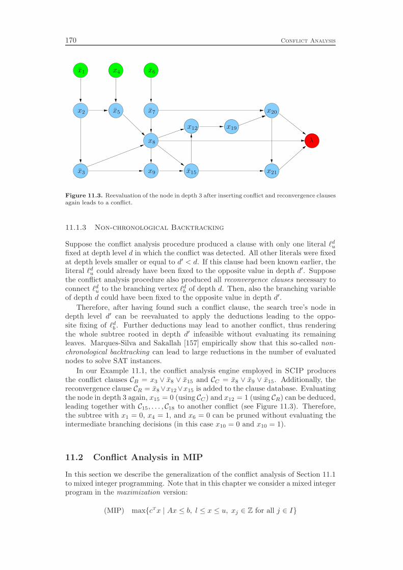
170 Conflict Analysis
replacemen
x1
x2
x3
x4
x5
x6
x7
x8
x9
x12
x15
x19
x20
x21
λ
Figure 11.3. Reevaluation of the node in depth 3 after inserting conflict and reconvergence clausesagain leads to a conflict.
11.1.3 Non-chronological Backtracking
Suppose the conflict analysis procedure produced a clause with only one literal ℓdufixed at depth level d in which the conflict was detected. All other literals were fixedat depth levels smaller or equal to d′ < d. If this clause had been known earlier, theliteral ℓdu could already have been fixed to the opposite value in depth d′. Supposethe conflict analysis procedure also produced all reconvergence clauses necessary toconnect ℓdu to the branching vertex ℓdb of depth d. Then, also the branching variableof depth d could have been fixed to the opposite value in depth d′.
Therefore, after having found such a conflict clause, the search tree’s node indepth level d′ can be reevaluated to apply the deductions leading to the oppo-site fixing of ℓdb . Further deductions may lead to another conflict, thus renderingthe whole subtree rooted in depth d′ infeasible without evaluating its remainingleaves. Marques-Silva and Sakallah [157] empirically show that this so-called non-chronological backtracking can lead to large reductions in the number of evaluatednodes to solve SAT instances.
In our Example 11.1, the conflict analysis engine employed in SCIP producesthe conflict clauses CB = x3 ∨ x8 ∨ x15 and CC = x8 ∨ x9 ∨ x15. Additionally, thereconvergence clause CR = x8∨x12∨x15 is added to the clause database. Evaluatingthe node in depth 3 again, x15 = 0 (using CC) and x12 = 1 (using CR) can be deduced,leading together with C15, . . . , C18 to another conflict (see Figure 11.3). Therefore,the subtree with x1 = 0, x4 = 1, and x6 = 0 can be pruned without evaluating theintermediate branching decisions (in this case x10 = 0 and x10 = 1).
11.2 Conflict Analysis in MIP
In this section we describe the generalization of the conflict analysis of Section 11.1to mixed integer programming. Note that in this chapter we consider a mixed integerprogram in the maximization version:
(MIP) max{cTx | Ax ≤ b, l ≤ x ≤ u, xj ∈ Z for all j ∈ I}
11.2. Conflict Analysis in MIP 171
with A ∈ Rm×n, b ∈ Rm, c, l, u ∈ Rn, and I ⊆ N = {1, . . . , n}. A branch-and-boundbased MIP solver decomposes the problem instance into subproblems typically bymodifying the bounds l and u of the variables. These branching decisions may entailfurther deductions on the bounds of other variables, which are generated by domainpropagation, see Chapter 7.
Suppose we detected a subproblem in the branch-and-bound search tree to beinfeasible, either because a deduction leads to a variable with empty domain orbecause the LP relaxation is infeasible. To analyze this conflict, we proceed in thesame fashion as in SAT solving: we construct a conflict graph, choose a cut in thisgraph, and produce a conflict constraint which consists of the variables in the conflictset, i.e., in the cut’s frontier. Because an MIP may contain non-binary variables, wehave to extend the concept of the conflict graph: it has to represent bound changesinstead of fixings of variables. This generalization is described in Section 11.2.1.
A conflict in SAT solving is always detected due to a single clause that becameempty during the Boolean constraint propagation process (see Section 11.1). Thisconflict-detecting clause provides the links from the vertices in the conflict graphthat represent fixings of variables to the conflict vertex λ. In contrast, in an LPbased branch-and-bound algorithm to solve mixed integer programs, infeasibility ofa subproblem is almost always detected due to the infeasibility of its LP relaxationor due to the LP exceeding the primal bound. In this case the LP relaxation asa whole is responsible for the infeasibility. There is no single conflict-detectingconstraint that defines the predecessors of the conflict vertex in the conflict graph.To cope with this situation, we have to analyze the LP in order to identify a subset ofthe bound changes that suffices to render the LP infeasible or bound-exceeding. Theconflict vertex can then be connected to the vertices of this subset. Section 11.2.2explains how to analyze infeasible LPs and how to identify an appropriate subset ofthe bound changes. The case of LPs having exceeded the objective bound is treatedin Section 11.2.3.
Note that the LP analysis is related to the separation of Dantzig cuts, see Bowmanand Nemhauser [53] or Rubin and Graves [195], which are known to be computation-ally ineffective. However, the latter include all non-basic variables of a fractionalLP solution, while the LP analysis selects only a (hopefully very small) subset ofthe variables in an infeasible or bound-exceeding solution as starting point for theconflict graph analysis.
After the conflict graph has been constructed, we have to choose a cut in thegraph in order to define the conflict set and the resulting conflict constraint. In thecase of a binary program, i.e., B = I = N , l = 0, u = 1, the conflict graph can beanalyzed by the same algorithms as described in Section 11.1 to produce a conflictclause Cf =
∨
ℓj∈Vfℓj . This clause can be linearized by the set covering constraint
∑
j:xj∈Vf
(1− xj) +∑
j:xj∈Vf
xj ≥ 1, (11.1)
and added to the MIP’s constraint set. However, in the presence of non-binaryvariables, the analysis of the conflict graph may produce a conflict set that containsbound changes on non-binary variables. In this case the conflict constraint cannot belinearized by the set covering constraint (11.1). Section 11.2.4 shows how non-binaryvariables can be incorporated into the conflict constraints.
172 Conflict Analysis
11.2.1 Generalized Conflict Graph
If general integer or continuous variables are present in the problem, a bound ona specific variable could have been changed more than once on the path from theroot node to the current subproblem in the search tree. A local bound change ona non-binary variable can be both reason and consequence of a deduction, similarto a fixing of a binary variable. Therefore, we generalize the concept of the conflictgraph: the vertices now represent bound changes instead of fixings. Note that therecan now exist multiple vertices corresponding to the same non-binary variable in theconflict graph, each vertex representing one change of the variable’s bounds.
Example 11.3. Consider the following constraints of an integer program with vari-ables x1, . . . , x7 ∈ {0, 1} and z1, . . . , z5 ∈ Z≥0.
2x1 + 3z1 +2z2 ≤ 9 (11.2)
+ 9x2 − z1 − 2z2 ≤ 0 (11.3)
− 3x2 + 5x3 − 3x4 ≤ 4 (11.4)
− 3x2 + 9x4 − 2z3 ≤ 6 (11.5)
+ 9x5 − z2 + 2z3 ≤ 8 (11.6)
− 4x6 − 7x7 + 2z3 ≤ 3 (11.7)
+ 5x7 − 2z2 ≤ 2 (11.8)
− x5 + 5x7 +4z2 − 5z3 ≤ 2 (11.9)
x1 − x2 + x3 − 2x5 + x6 − z1 − 2z2 + z3 − 2z4 + 4z5 ≤ 1 (11.10)
+ 2x2 − x4 + 3x5 − 2x6 − z1 +5z2 + z3 +2z4 − 6z5 ≤ 2 (11.11)
−2x1 − 2x3 + x4 + x5 + z1 +2z2 − 2z3 +2z4 − 2z5 ≤ 1 (11.12)
By the basic bound-strengthening techniques of Savelsbergh [199], see also Chapter 7,we can deduce upper bounds z1 ≤ 3, z2 ≤ 4, z3 ≤ 6, z4 ≤ 23, and z5 ≤ 15on the general integer variables. Assume we branched on x1 = 1. By applyingbound-strengthening on constraint (11.2) we can deduce z1 ≤ 2 and z2 ≤ 3 (seeFigure 11.4). Using constraint (11.3) and the new bounds on z1 and z2 it followsx2 = 0. By inserting the bound on z2 into constraint (11.6) we can also infer z3 ≤ 5.After branching on x3 = 1 and x6 = 0 and applying the deductions that follow fromthese branching decisions we arrive at the situation depicted in Figure 11.4 with theLP relaxation being infeasible. Note that the non-binary variables zi appear morethan once in the conflict graph. For example, the upper bound of z3 was changedonce and the lower bound was changed twice. The implications on variables z4 andz5 are not included in the figure. The bounds of these variables can be tightened to7 ≤ z4 ≤ 11 and 4 ≤ z5 ≤ 6.
We use the following notation in the rest of the chapter. Let BL = {B1, . . . , BK}with hyperplanes
Bk = Lµk
jk:= {x ∈ Rn | xjk
≥ µk} or
Bk = Uµk
jk:= {x ∈ Rn | xjk
≤ µk},
with 1 ≤ jk ≤ n and ljk≤ µk ≤ ujk
for k = 1, . . . ,K. The set BL corresponds tothe additional bounds imposed on the variables in the local subproblem. Thus, thesubproblem is defined as
(MIP′) max{
cTx | Ax ≤ b, l ≤ x ≤ u, xj ∈ Z for all j ∈ I, x ∈⋂
B∈BL
B}
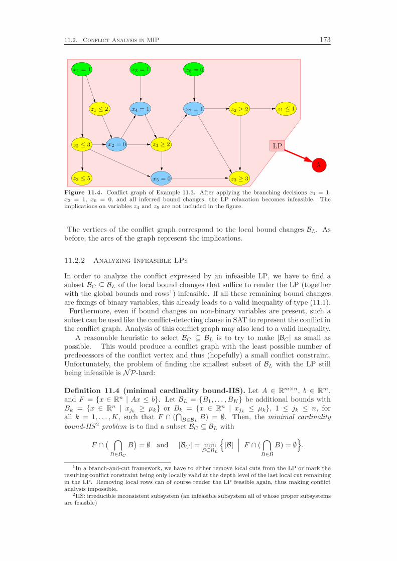
11.2. Conflict Analysis in MIP 173
x1 = 1
x2 = 0
x3 = 1
x4 = 1
x5 = 0
x6 = 0
x7 = 1z1 ≤ 2
z2 ≤ 3
z3 ≤ 5
z3 ≥ 2
z2 ≥ 2
z3 ≥ 3
z1 ≤ 1
λ
LP
Figure 11.4. Conflict graph of Example 11.3. After applying the branching decisions x1 = 1,x3 = 1, x6 = 0, and all inferred bound changes, the LP relaxation becomes infeasible. Theimplications on variables z4 and z5 are not included in the figure.
The vertices of the conflict graph correspond to the local bound changes BL. Asbefore, the arcs of the graph represent the implications.
11.2.2 Analyzing Infeasible LPs
In order to analyze the conflict expressed by an infeasible LP, we have to find asubset BC ⊆ BL of the local bound changes that suffice to render the LP (togetherwith the global bounds and rows1) infeasible. If all these remaining bound changesare fixings of binary variables, this already leads to a valid inequality of type (11.1).
Furthermore, even if bound changes on non-binary variables are present, such asubset can be used like the conflict-detecting clause in SAT to represent the conflict inthe conflict graph. Analysis of this conflict graph may also lead to a valid inequality.
A reasonable heuristic to select BC ⊆ BL is to try to make |BC | as small aspossible. This would produce a conflict graph with the least possible number ofpredecessors of the conflict vertex and thus (hopefully) a small conflict constraint.Unfortunately, the problem of finding the smallest subset of BL with the LP stillbeing infeasible is NP-hard:
Definition 11.4 (minimal cardinality bound-IIS). Let A ∈ Rm×n, b ∈ Rm,and F = {x ∈ Rn | Ax ≤ b}. Let BL = {B1, . . . , BK} be additional bounds withBk = {x ∈ Rn | xjk
≥ µk} or Bk = {x ∈ Rn | xjk≤ µk}, 1 ≤ jk ≤ n, for
all k = 1, . . . ,K, such that F ∩ (⋂
B∈BLB) = ∅. Then, the minimal cardinality
bound-IIS2 problem is to find a subset BC ⊆ BL with
F ∩( ⋂
B∈BC
B)
= ∅ and |BC | = minB⊆BL
{
|B|∣∣∣ F ∩ (
⋂
B∈B
B) = ∅}
.
1In a branch-and-cut framework, we have to either remove local cuts from the LP or mark theresulting conflict constraint being only locally valid at the depth level of the last local cut remainingin the LP. Removing local rows can of course render the LP feasible again, thus making conflictanalysis impossible.
2IIS: irreducible inconsistent subsystem (an infeasible subsystem all of whose proper subsystemsare feasible)
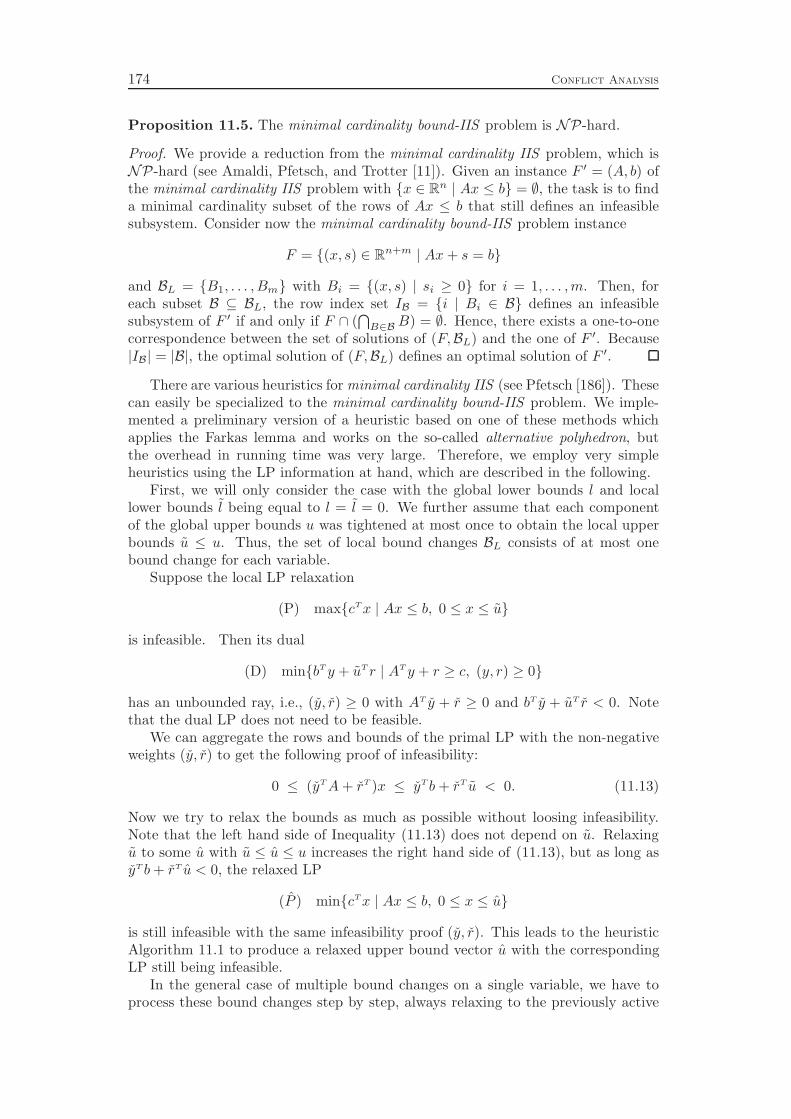
174 Conflict Analysis
Proposition 11.5. The minimal cardinality bound-IIS problem is NP-hard.
Proof. We provide a reduction from the minimal cardinality IIS problem, which isNP-hard (see Amaldi, Pfetsch, and Trotter [11]). Given an instance F ′ = (A, b) ofthe minimal cardinality IIS problem with {x ∈ Rn | Ax ≤ b} = ∅, the task is to finda minimal cardinality subset of the rows of Ax ≤ b that still defines an infeasiblesubsystem. Consider now the minimal cardinality bound-IIS problem instance
F = {(x, s) ∈ Rn+m | Ax+ s = b}
and BL = {B1, . . . , Bm} with Bi = {(x, s) | si ≥ 0} for i = 1, . . . ,m. Then, foreach subset B ⊆ BL, the row index set IB = {i | Bi ∈ B} defines an infeasiblesubsystem of F ′ if and only if F ∩ (
⋂
B∈B B) = ∅. Hence, there exists a one-to-onecorrespondence between the set of solutions of (F,BL) and the one of F ′. Because|IB| = |B|, the optimal solution of (F,BL) defines an optimal solution of F ′.
There are various heuristics for minimal cardinality IIS (see Pfetsch [186]). Thesecan easily be specialized to the minimal cardinality bound-IIS problem. We imple-mented a preliminary version of a heuristic based on one of these methods whichapplies the Farkas lemma and works on the so-called alternative polyhedron, butthe overhead in running time was very large. Therefore, we employ very simpleheuristics using the LP information at hand, which are described in the following.
First, we will only consider the case with the global lower bounds l and locallower bounds l being equal to l = l = 0. We further assume that each componentof the global upper bounds u was tightened at most once to obtain the local upperbounds u ≤ u. Thus, the set of local bound changes BL consists of at most onebound change for each variable.
Suppose the local LP relaxation
(P) max{cTx | Ax ≤ b, 0 ≤ x ≤ u}
is infeasible. Then its dual
(D) min{bTy + uT r | ATy + r ≥ c, (y, r) ≥ 0}
has an unbounded ray, i.e., (y, r) ≥ 0 with AT y + r ≥ 0 and bT y + uT r < 0. Notethat the dual LP does not need to be feasible.
We can aggregate the rows and bounds of the primal LP with the non-negativeweights (y, r) to get the following proof of infeasibility:
0 ≤ (yTA+ rT )x ≤ yT b+ rT u < 0. (11.13)
Now we try to relax the bounds as much as possible without loosing infeasibility.Note that the left hand side of Inequality (11.13) does not depend on u. Relaxingu to some u with u ≤ u ≤ u increases the right hand side of (11.13), but as long asyT b+ rT u < 0, the relaxed LP
(P ) min{cTx | Ax ≤ b, 0 ≤ x ≤ u}
is still infeasible with the same infeasibility proof (y, r). This leads to the heuristicAlgorithm 11.1 to produce a relaxed upper bound vector u with the correspondingLP still being infeasible.
In the general case of multiple bound changes on a single variable, we have toprocess these bound changes step by step, always relaxing to the previously active

11.2. Conflict Analysis in MIP 175
Algorithm 11.1 Infeasible LP Analysis
Input : An infeasible LP max{cTx | Ax ≤ b, 0 ≤ x ≤ u ≤ u} with dual ray (y, r).
Output : Relaxed upper bounds u ≥ u such that the LP is still infeasible.
1. Set u := u, and calculate the infeasibility measure d := yT b+ rT u < 0.
2. Select a variable j with uj < uj and dj := d + rj(uj − uj) < 0. If no suchvariable exists, stop.
3. Set uj := uj , update d := dj , and go to Step 2.
bound. In the presence of non-zero lower bounds the reduced costs r may also benegative. In this case, we can split up the reduced cost values into r = ru − rl
with ru, rl ≥ 0. It follows from the Farkas lemma that ru · rl = 0. The infeasibilitymeasure d of the dual ray has to be defined in Step 1 as d := yT b+ (ru)T u+ (rl)T l.A local lower bound l can be relaxed in the same way as an upper bound u, whereu has to be replaced by l in the formulas of Steps 2 and 3.
Example 11.6 (continued from Example 11.3). After applying the deductionson the bounds of the variables in Example 11.3, the LP relaxation is infeasible. Lety(i) denote the dual variable of constraint (i) and rj the reduced cost value of variablej. Then the dual ray y(11.10) = 2, y(11.11) = 1, y(11.12) = 1, rz1
= 2, rz2= −3,
rz3= −1, and the remaining coefficients set to zero proves the infeasibility of the
LP. In Step 1 of Algorithm 11.1 the infeasibility measure is calculated as
d = y(11.10)b(11.10) + y(11.11)b(11.11) + y(11.12)b(11.12) + ruz1uz1− rl
z2lz2− rl
z3lz3
= 2 · 1 + 1 · 2 + 1 · 1 + 2 · 1 − 3 · 2 − 1 · 3
= −2.
In Step 2, all local bounds except the upper bound of z1 and the lower bounds ofz2 and z3 can be relaxed to the corresponding global bounds, because their reducedcost values in the dual ray are zero. Additionally, the lower bound of z3 can berelaxed from 3 to 2, which was the lower bound before z3 ≥ 3 was deduced. Thisrelaxation increases d by 1 to d = −1. No further relaxations are possible withoutincreasing d to d ≥ 0. Thus, the local bounds z1 ≤ 1, z2 ≥ 2, and z3 ≥ 2 areidentified as initial reason for the conflict, and the “global” arc from the LP to theconflict vertex in Figure 11.4 can be replaced by three arcs as shown in Figure 11.5.The 1-FUIP scheme applied to the resulting conflict graph yields the cut labeled
’A’ and the conflict constraint
(z2 ≤ 1) ∨ (z3 ≤ 1).
Note that the involved variables z2 and z3 are non-binary. Section 11.2.4 shows howto proceed in this situation.
11.2.3 Analyzing LPs Exceeding the Primal Bound
In principle, the case of an LP exceeding the primal bound can be handled as inthe previous section by adding an appropriate objective bound inequality to theconstraint system. In the implementation, however, we use the dual solution directly
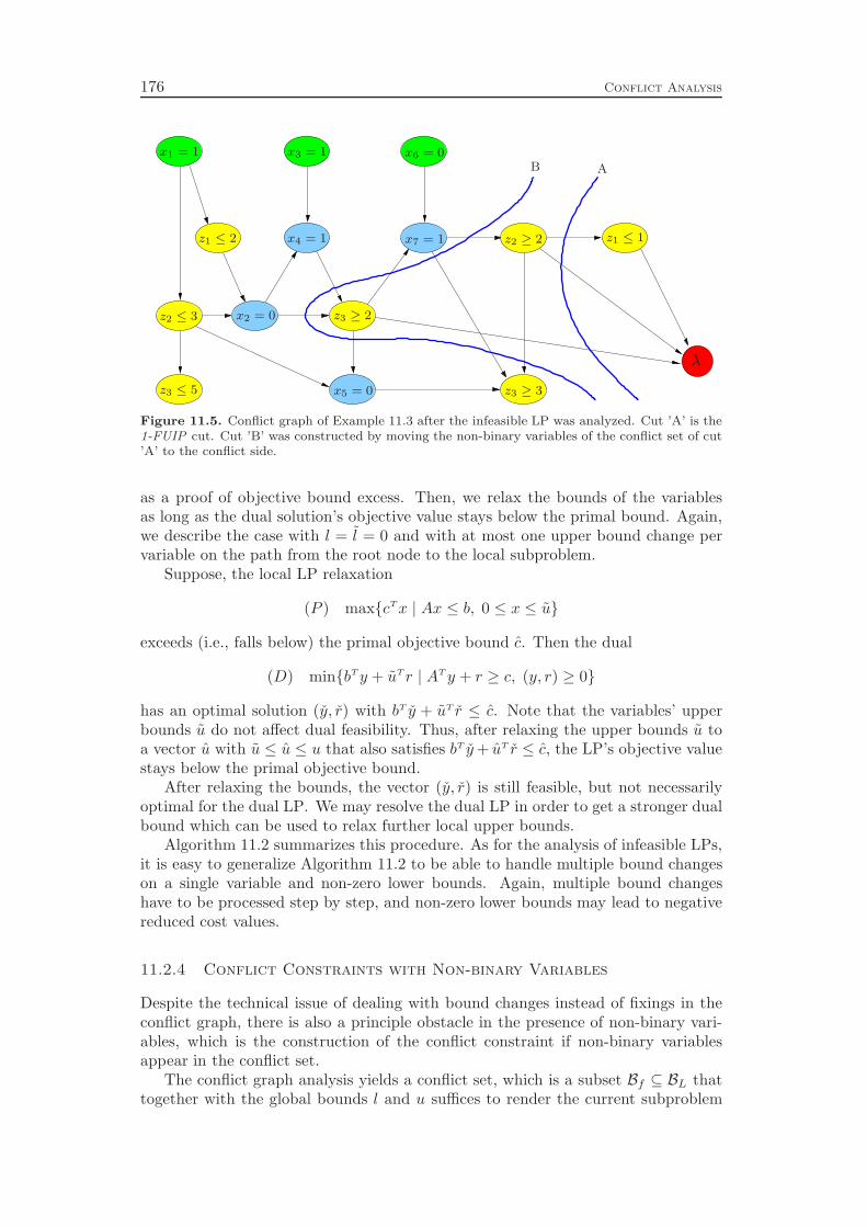
176 Conflict Analysis
x1 = 1
x2 = 0
x3 = 1
x4 = 1
x5 = 0
x6 = 0
x7 = 1z1 ≤ 2
z2 ≤ 3
z3 ≤ 5
z3 ≥ 2
z2 ≥ 2
z3 ≥ 3
z1 ≤ 1
λ
AB
Figure 11.5. Conflict graph of Example 11.3 after the infeasible LP was analyzed. Cut ’A’ is the1-FUIP cut. Cut ’B’ was constructed by moving the non-binary variables of the conflict set of cut’A’ to the conflict side.
as a proof of objective bound excess. Then, we relax the bounds of the variablesas long as the dual solution’s objective value stays below the primal bound. Again,we describe the case with l = l = 0 and with at most one upper bound change pervariable on the path from the root node to the local subproblem.
Suppose, the local LP relaxation
(P ) max{cTx | Ax ≤ b, 0 ≤ x ≤ u}
exceeds (i.e., falls below) the primal objective bound c. Then the dual
(D) min{bTy + uTr | ATy + r ≥ c, (y, r) ≥ 0}
has an optimal solution (y, r) with bT y + uT r ≤ c. Note that the variables’ upperbounds u do not affect dual feasibility. Thus, after relaxing the upper bounds u toa vector u with u ≤ u ≤ u that also satisfies bT y+ uT r ≤ c, the LP’s objective valuestays below the primal objective bound.
After relaxing the bounds, the vector (y, r) is still feasible, but not necessarilyoptimal for the dual LP. We may resolve the dual LP in order to get a stronger dualbound which can be used to relax further local upper bounds.
Algorithm 11.2 summarizes this procedure. As for the analysis of infeasible LPs,it is easy to generalize Algorithm 11.2 to be able to handle multiple bound changeson a single variable and non-zero lower bounds. Again, multiple bound changeshave to be processed step by step, and non-zero lower bounds may lead to negativereduced cost values.
11.2.4 Conflict Constraints with Non-binary Variables
Despite the technical issue of dealing with bound changes instead of fixings in theconflict graph, there is also a principle obstacle in the presence of non-binary vari-ables, which is the construction of the conflict constraint if non-binary variablesappear in the conflict set.
The conflict graph analysis yields a conflict set, which is a subset Bf ⊆ BL thattogether with the global bounds l and u suffices to render the current subproblem
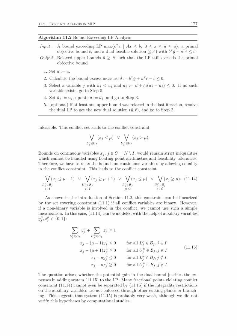
11.2. Conflict Analysis in MIP 177
Algorithm 11.2 Bound Exceeding LP Analysis
Input : A bound exceeding LP max{cTx | Ax ≤ b, 0 ≤ x ≤ u ≤ u}, a primalobjective bound c, and a dual feasible solution (y, r) with bT y + uT r ≤ c.
Output : Relaxed upper bounds u ≥ u such that the LP still exceeds the primalobjective bound.
1. Set u := u.
2. Calculate the bound excess measure d := bT y + uT r − c ≤ 0.
3. Select a variable j with uj < uj and dj := d + rj(uj − uj) ≤ 0. If no suchvariable exists, go to Step 5.
4. Set uj := uj , update d := dj , and go to Step 3.
5. (optional) If at least one upper bound was relaxed in the last iteration, resolvethe dual LP to get the new dual solution (y, r), and go to Step 2.
infeasible. This conflict set leads to the conflict constraint
∨
Lµj ∈Bf
(xj < µ) ∨∨
Uµj ∈Bf
(xj > µ).
Bounds on continuous variables xj , j ∈ C = N \ I, would remain strict inequalitieswhich cannot be handled using floating point arithmetics and feasibility tolerances.Therefore, we have to relax the bounds on continuous variables by allowing equalityin the conflict constraint. This leads to the conflict constraint
∨
Lµj ∈Bf
j∈I
(xj ≤ µ− 1) ∨∨
Uµj ∈Bf
j∈I
(xj ≥ µ+ 1) ∨∨
Lµj ∈Bf
j∈C
(xj ≤ µ) ∨∨
Uµj ∈Bf
j∈C
(xj ≥ µ). (11.14)
As shown in the introduction of Section 11.2, this constraint can be linearizedby the set covering constraint (11.1) if all conflict variables are binary. However,if a non-binary variable is involved in the conflict, we cannot use such a simplelinearization. In this case, (11.14) can be modeled with the help of auxiliary variablesyµ
j , zµj ∈ {0, 1}:
∑
Lµj ∈Bf
yµj +
∑
Uµj ∈Bf
zµj ≥ 1
xj − (µ− 1)yµj ≤ 0 for all Lµ
j ∈ Bf , j ∈ I
xj − (µ+ 1)zµj ≥ 0 for all Uµ
j ∈ Bf , j ∈ I
xj − µyµj ≤ 0 for all Lµ
j ∈ Bf , j /∈ I
xj − µzµj ≥ 0 for all Uµ
j ∈ Bf , j /∈ I
(11.15)
The question arises, whether the potential gain in the dual bound justifies the ex-penses in adding system (11.15) to the LP. Many fractional points violating conflictconstraint (11.14) cannot even be separated by (11.15) if the integrality restrictionson the auxiliary variables are not enforced through other cutting planes or branch-ing. This suggests that system (11.15) is probably very weak, although we did notverify this hypotheses by computational studies.
178 Conflict Analysis
We have the following two possibilities to avoid adding system (11.15) to the LP:either we use conflict constraints involving non-binary variables only for domainpropagation but not for cutting plane separation, or we prevent the generation ofconflict constraints with non-binary variables. The former demands the possibility ofincluding non-linear constraints into the underlying MIP framework. This is possiblesince SCIP provides support for arbitrary constraints. For the latter option wehave to modify the cut selection rules in the conflict graph analysis such that thenon-binary variables are not involved in the resulting conflict set. This can beachieved by moving the bound changes on non-binary variables from the reasonside’s frontier to the conflict side of the cut. The following example illustrates thisidea.
Example 11.7 (continued from Examples 11.3 and 11.6). Figure 11.5 showsthe conflict graph of Example 11.3 after branching on x1 = 1, x3 = 1, and x6 = 0.The analysis of the LP relaxation identified z1 ≤ 1, z2 ≥ 2, and z3 ≥ 2 as sufficient tocause an infeasibility in the LP (see Example 11.6). The 1-FUIP cut selection schemeleads to the cut labeled ’A’ in the figure. The corresponding conflict constraint is
(z2 ≤ 1) ∨ (z3 ≤ 1).
Because there are non-binary variables involved in the conflict constraint, it cannotbe linearized by the set covering constraint (11.1). To avoid the introduction of theauxiliary variables of System (11.15), the bound changes z2 ≥ 2 and z3 ≥ 2 are putto the conflict side, resulting in cut ’B’. Thus, the conflict constraint that is addedto the constraint database is
(x2 = 1) ∨ (x4 = 0) ∨ (x7 = 0),
which can be written as
x2 + (1− x4) + (1− x7) ≥ 1
in terms of a set covering constraint.
Since branching vertices must be located on the reason side, the bound changesrepresenting branching decisions on non-binary variables cannot be moved to theconflict side. In this case, we can just remove the bound change from the conflictset in order to obtain a set covering conflict constraint. However, we thereby destroythe global validity of the resulting conflict clause. The clause can therefore only beadded to the local subtree which is rooted at the node where the bound change onthe non-binary variable was applied.
11.3 Computational Results
In the following, we present the computational experiments that we conducted inorder to assess the performance impact of conflict analysis on solving mixed integerprograms. With the parameter settings we used for the experiments, we produce oneFUIP conflict constraint for every depth level in the conflict graph, see Section 11.1.1.This includes the 1-FUIP and All-FUIP schemes as extreme cases. In addition, wegenerate all reconvergence constraints, see Section 11.1.2, that are needed to link theFUIPs of the individual depth levels to the respective branching vertex. However, we
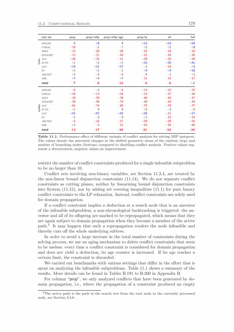
11.3. Computational Results 179
test set prop prop/inflp prop/inflp/age prop/lp all fullti
me
miplib 0 +6 0 +12 +14 +24
coral −10 −1 −7 +2 +2 +8
milp −13 −26 −28 −31 −24 −18
enlight −11 −21 −49 −21 −26 −26
alu −28 −35 −11 −39 −39 −38
fctp +1 +2 +1 +23 +20 +41
acc +19 +21 +17 −2 −19 +5
fc +1 +1 −1 +9 +9 +18
arcset +1 −6 −6 −4 −1 +1
mik +7 +4 +7 −11 −15 −17
total −7 −8 −12 −8 −6 +1
no
des
miplib −6 −1 −9 −14 −10 −15
coral −20 −13 −29 −22 −27 −36
milp −16 −29 −36 −48 −45 −47
enlight −29 −48 −79 −49 −49 −49
alu −61 −74 −80 −75 −78 −77
fctp +1 0 0 +2 −3 −8
acc +51 +57 +52 +20 −21 +17
fc −1 −3 −3 +1 −15 −24
arcset −5 −16 −17 −29 −29 −34
mik +1 −5 −12 −53 −55 −60
total −14 −17 −28 −31 −32 −36
Table 11.1. Performance effect of different variants of conflict analysis for solving MIP instances.The values denote the percental changes in the shifted geometric mean of the runtime (top) andnumber of branching nodes (bottom) compared to disabling conflict analysis. Positive values rep-resent a deterioration, negative values an improvement.
restrict the number of conflict constraints produced for a single infeasible subproblemto be no larger than 10.
Conflict sets involving non-binary variables, see Section 11.2.4, are treated bythe non-linear bound disjunction constraints (11.14). We do not separate conflictconstraints as cutting planes, neither by linearizing bound disjunction constraintsinto System (11.15), nor by adding set covering inequalities (11.1) for pure binaryconflict constraints to the LP relaxation. Instead, conflict constraints are solely usedfor domain propagation.
If a conflict constraint implies a deduction at a search node that is an ancestorof the infeasible subproblem, a non-chronological backtracking is triggered: the an-cestor and all of its offspring are marked to be repropagated, which means that theyare again subject to domain propagation when they become a member of the activepath.3 It may happen that such a repropagation renders the node infeasible andthereby cuts off the whole underlying subtree.
In order to avoid a large increase in the total number of constraints during thesolving process, we use an aging mechanism to delete conflict constraints that seemto be useless: every time a conflict constraint is considered for domain propagationand does not yield a deduction, its age counter is increased. If its age reaches acertain limit, the constraint is discarded.
We carried out benchmarks with various settings that differ in the effort that isspent on analyzing the infeasible subproblems. Table 11.1 shows a summary of theresults. More details can be found in Tables B.191 to B.200 in Appendix B.
For column “prop”, we only analyzed conflicts that have been generated by do-main propagation, i.e., where the propagation of a constraint produced an empty
3The active path is the path in the search tree from the root node to the currently processednode, see Section 3.3.6.
180 Conflict Analysis
domain for a variable. This already achieves a significant performance improvementfor most of the test sets. Most notably, the average number of branch-and-boundnodes needed to prove the infeasibility of the alu instances reduces by more than60 %, which translates into a runtime reduction of almost 30 %.
Column “prop/inflp” shows the results for applying Algorithm 11.1 to analyzesubproblems for which the LP relaxation was infeasible in addition to the propaga-tion conflict analysis of column “prop”. The results are quite similar to using onlypropagation conflict analysis: for some test sets, namely milp, enlight, alu, andarcset, the performance improves, but one can observe a considerable deteriorationon the miplib and coral instances. The differences in the average number of nodesfor the “prop” and “prop/inflp” settings are strongly correlated to the differencesin the solving time. This indicates that the computational costs for the additionalanalysis of infeasible LP relaxations are negligible.
The “prop/inflp/age” settings differ from the ones used in column “prop/inflp” inthe aging rule that is used to discard seemingly useless conflict constraints. Here,conflict constraints are kept longer, which leads to a larger overhead in the constraintmanagement but also to more deductions in domain propagation. It turns outthat this less aggressive constraint removal policy does not only reduce the averagenumber of nodes but also the average solving time for almost all test sets. The onlycounter-examples are the alu and mik instances. In particular for the alu test set,the additional reduction in the number of nodes does not compensate the highercosts for constraint management and propagation: the average number of nodes is25 % smaller than for the default aging policy, but the average runtime is 37 % larger.
In addition to conflicting propagations and infeasible LP relaxations, the “prop/lp”settings employ Algorithm 11.2 to analyze LPs that exceed the primal bound. Foreach conflict, the optional LP resolving in Step 5 is executed at most twice, eachtime performing at most 10 dual simplex iterations. Compared to the “prop/inflp”settings, analyzing bound-exceeding LPs yields an even larger reduction in the aver-age number of nodes to solve the instances. Unfortunately, it does not improve theoverall runtime performance.
The results on the alu instances deserve an explanation. As noted earlier, theseMIP instances are infeasible. Therefore, there will never be any incumbent solutionduring the solving process, and it seems strange that the results differ if boundexceeding LPs are analyzed. However, even though there is no feasible solution athand, SCIP sets a cutoff bound for the LP solver, namely the trivial bound
c⋆ ≤ max{cTx | l ≤ x ≤ u} =∑
cj<0
cjlj +∑
cj>0
cjuj .
Therefore, it may happen that the dual simplex algorithm hits the cutoff boundbefore it detects the infeasibility of the LP relaxation.
The settings used in column “all” extend the conflict analysis of “prop/lp” toinfeasible or bound-exceeding LP relaxations encountered during the strong branch-ing evaluation of branching candidates, see Section 5.4. Compared to “prop/lp”, anotable difference in the number of branching nodes can only be observed for theacc and fc instances. The average runtime performance gets slightly worse by usingstrong branching LP conflict analysis, which is mostly due to the inferior result onthe milp test set.
Analyzing infeasible or bound-exceeding strong branching LPs involves a tech-nical issue that is related to the API of Cplex. Strong branching is performedby calling the special purpose method CPXstrongbranch(). Unfortunately, this
11.3. Computational Results 181
method does not return the necessary dual information that is needed to analyzean infeasible or bound-exceeding strong branching LP. Therefore, we have to solvethese LPs again with the regular CPXdualopt() method before we can analyze theconflict. This imposes a small artificial runtime overhead, but it is unlikely that thisoverhead influences the benchmark results in a significant way.
Finally, the “full” conflict analysis settings achieve the largest reduction in theaverage number of branching nodes. In these settings, we produce conflict constraintsfor conflicting domain propagations, infeasible and bound-exceeding LP relaxations,and strong branching LPs. In Algorithm 11.2, which analyzes bound-exceeding LPs,we apply the LP resolving Step 5 as often as possible and do not impose any limiton the number of simplex iterations. Additionally, there is no limit on the numberof constraints produced for each conflict.
Compared to the “all” settings, this very aggressive use of conflict analysis in-creases the average runtime on almost all test sets, with the most notable perfor-mance deterioration on the miplib, fctp, acc, and fc instances. With the exceptionof alu and acc, however, the average number of nodes needed to solve the instancesis reduced. This indicates that such an extensive use of conflict analysis is too timeconsuming and leads to an unreasonable overhead in the constraint management.
We conclude from our experiments that conflict analysis is indeed a useful toolto improve the performance of MIP solvers. The largest speedup can be achievedfor infeasible MIPs like the alu instances and models of combinatorial nature as theones in the enlight test set. The details of the implementation, however, have to beconsidered carefully in order to avoid a large runtime overhead for the analysis andthe conflict constraint management. In particular, the policy to discard seeminglyuseless conflict constraints seems to be an important factor.


Part III
Chip Design Verification
183

Chapter 12
Introduction
This part of the thesis addresses the property checking problem arising in the formalverification of integrated circuit designs. This problem was treated in work pack-age 1 of the BMBF1 project Valse-XT2 in cooperation with Infineon3, OneSpinSolutions4, and TU Kaiserslautern5. The introduction is joint work with RaikBrinkmann and Markus Wedler.
A recent trend in the semiconductor industry is to produce so-called Systems-on-Chips (SoCs). These are circuits which integrate large parts of the functionalityof complete electronic systems. They are employed in cell phones, car controls,digital televisions, network processors, video games, and many other devices (see,e.g., Jerraya and Wolf [123]).
Due to the complexity of SoCs, it is a very challenging task to ensure the cor-rectness of the chip design. The following quotation is taken from ITRS 2005 [120],the International Technology Roadmap for Semiconductors:
Design verification is the task of establishing that a given design accu-rately implements the intended behavior. Today, the verification of mod-ern computing systems has grown to dominate the cost of electronic sys-tem design, often with limited success, as designs continue to be releasedwith latent bugs. In fact, in many application domains, the verificationportion has become the predominant component of a project development,in terms of time, cost and human resources dedicated to it. In currentprojects verification engineers outnumber designers, with this ratio reach-ing two or three to one for the most complex designs. Design conceptionand implementation are becoming mere preludes to the main activity ofverification.
According to Infineon [207], 60 % to 80 % of the expenses in SoC chip design arespent on verification. The goal of the Valse-XT project was to improve the currentstate-of-the-art in chip design verification in order to cope with the ever increasingcomplexity of integrated circuits.
SoCs are composed of several smaller circuit modules. It is a natural idea toverify the correctness of the chip design in a hierarchical fashion. This imposesvery strong quality restrictions on the individual modules. For example, if the SoCcontains 100 modules with each of them behaving correctly on 99.9 % of the inputpatterns, the behavior of the SoC as a whole is only correct in about 90 % of thecases (at least if the modules fail on different inputs). Therefore, it is necessary toprove the correctness of the individual modules, thereby showing 100 % correctnessof their input-output behavior.
1Bundesministerium für Bildung und Forschung, http://www.bmbf.de2BMBF-Ekompass Project No. 01 M 3069 A, http://www.edacentrum.de/ekompass/3http://www.infineon.com4http://www.onespin-solutions.com5http://www-eda.eit.uni-kl.de
185
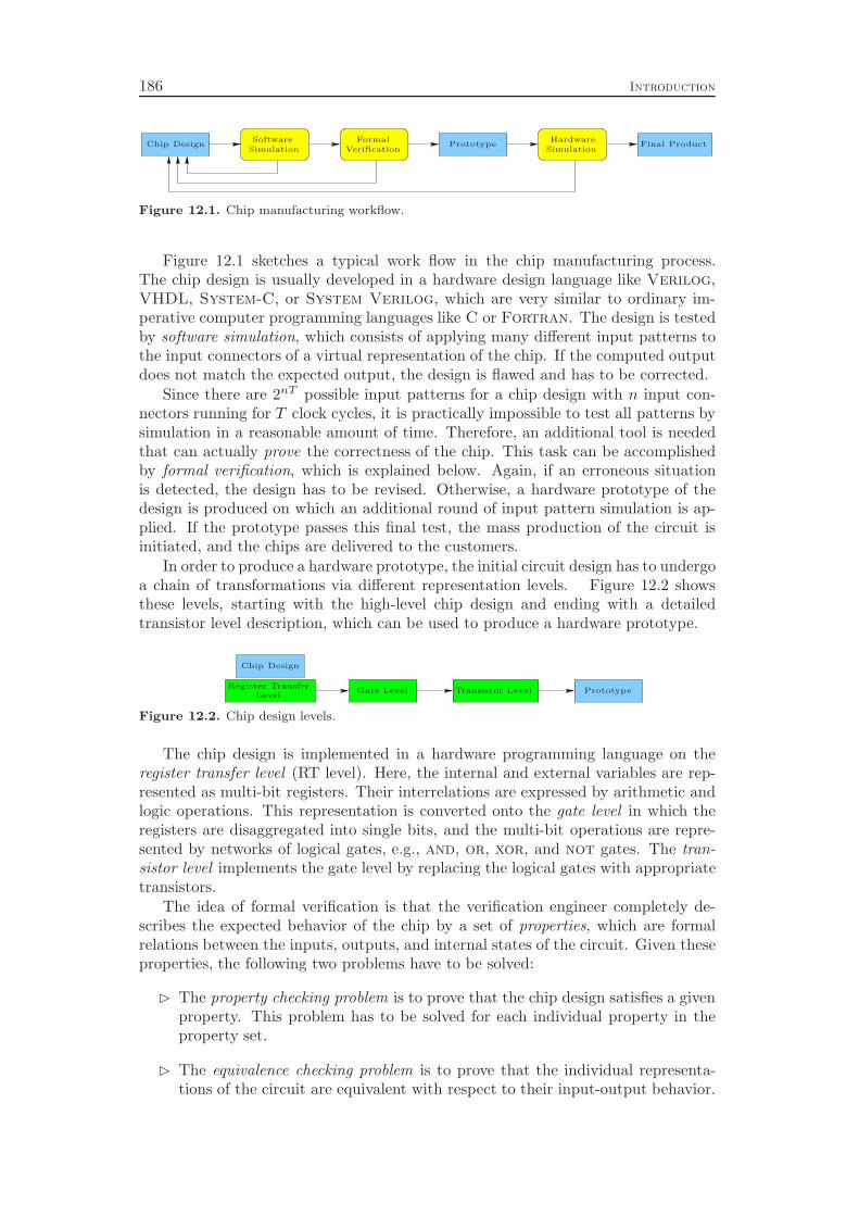
186 Introduction
Chip DesignSoftware
SimulationSimulation
Formal
VerificationPrototype
HardwareFinal Product
Figure 12.1. Chip manufacturing workflow.
Figure 12.1 sketches a typical work flow in the chip manufacturing process.The chip design is usually developed in a hardware design language like Verilog,VHDL, System-C, or System Verilog, which are very similar to ordinary im-perative computer programming languages like C or Fortran. The design is testedby software simulation, which consists of applying many different input patterns tothe input connectors of a virtual representation of the chip. If the computed outputdoes not match the expected output, the design is flawed and has to be corrected.
Since there are 2nT possible input patterns for a chip design with n input con-nectors running for T clock cycles, it is practically impossible to test all patterns bysimulation in a reasonable amount of time. Therefore, an additional tool is neededthat can actually prove the correctness of the chip. This task can be accomplishedby formal verification, which is explained below. Again, if an erroneous situationis detected, the design has to be revised. Otherwise, a hardware prototype of thedesign is produced on which an additional round of input pattern simulation is ap-plied. If the prototype passes this final test, the mass production of the circuit isinitiated, and the chips are delivered to the customers.
In order to produce a hardware prototype, the initial circuit design has to undergoa chain of transformations via different representation levels. Figure 12.2 showsthese levels, starting with the high-level chip design and ending with a detailedtransistor level description, which can be used to produce a hardware prototype.
Chip Design
Register Transfer
LevelGate Level Transistor Level Prototype
Figure 12.2. Chip design levels.
The chip design is implemented in a hardware programming language on theregister transfer level (RT level). Here, the internal and external variables are rep-resented as multi-bit registers. Their interrelations are expressed by arithmetic andlogic operations. This representation is converted onto the gate level in which theregisters are disaggregated into single bits, and the multi-bit operations are repre-sented by networks of logical gates, e.g., and, or, xor, and not gates. The tran-sistor level implements the gate level by replacing the logical gates with appropriatetransistors.
The idea of formal verification is that the verification engineer completely de-scribes the expected behavior of the chip by a set of properties, which are formalrelations between the inputs, outputs, and internal states of the circuit. Given theseproperties, the following two problems have to be solved:
⊲ The property checking problem is to prove that the chip design satisfies a givenproperty. This problem has to be solved for each individual property in theproperty set.
⊲ The equivalence checking problem is to prove that the individual representa-tions of the circuit are equivalent with respect to their input-output behavior.
Introduction 187
The equivalence ensures that no errors are introduced during the transforma-tion chain from chip design to transistor level.
If the chip design satisfies all of the given properties and all representations areequivalent, the chip design and the transistor model of the hardware circuit areprovably correct. In the remainder of the thesis we focus on the property checkingproblem.
Constraint Integer Programming Approach
Properties can be defined in a language similar to the ones used to design the chip.Like the chip design, a property can be transformed to the different representationlevels shown in Figure 12.2. Given that the equivalence checking has already beensuccessfully accomplished, one can deal with the property checking problem at anysuitable representation level.
Current state-of-the-art property checking algorithms operate on the gate leveldescription. At this level, the design and the property can be converted into aninstance of the satisfiability problem (see Section 1.2), which is then solved by ablack-box SAT solver. In order to obtain a finite set of variables, one has to applybounded model checking (Biere et al. [42]), which means to define a sufficiently largebut finite time horizon T . Biere et al. fix the initial state at t = 0 to be the resetstate of the circuit. In contrast, we leave the initial state of the circuit undefined,such that we can also identify errors that can only be reached after more than Ttime steps from the reset stage. The disadvantage is that we may report errors thatresult from an initial state t = 0, which is not reachable from the reset state andthat can therefore never appear.
The reduction of the property checking problem to a SAT instance facilitatesformal verification of industrial circuit designs far beyond the scope of classicalmodel checking techniques like BDD6 based approaches (see Biere et al. [43] orBjesse et al. [47]). However, it is well known that SAT solvers have problems whendealing with instances derived from the verification of arithmetic circuits (as opposedto logic oriented circuits). Hence, although SAT based property checking can oftenbe applied successfully to the control part of a design, it typically fails on data pathswith large arithmetic blocks.
This motivated the development of word level solvers using integer program-ming (IP) [55, 83, 222] or constraint programming (CP) [221] that can be appliedat the register transfer level where the structure of the arithmetic operations is stillvisible. Current IP and CP solvers, however, do not learn conflict clauses during thesearch like SAT solvers (see Chapter 11). Therefore, they usually perform poorly onthe control part of a design. Moreover, in order to obtain highly optimized circuitsdesigners often implement arithmetic functions at the bit level such that word levelsolvers are not adequate. Thus, a combination of word level and Boolean solvers hasto be developed. Two promising ways of integrating IP and SAT have been proposedby Chai and Kuehlmann [59] and Audemard et al. [27]. Chai and Kuehlmann usepseudo-Boolean constraints (PBCs) as clauses in a branch-and-bound based solver,and Audemard et al. use linear equations as propositions. The reasoning of PBCsolvers, however, is still limited to the bit level and the benefit of the stronger searchspace pruning due to learned PBCs usually does not justify the overhead for han-dling these more complex constraints. On the other hand, using IP techniques at
6binary decision diagram, see Akers [8], Bryant [57], or Madre and Billon [152]
188 Introduction
the leaves of a decision tree without learning from infeasibilities sacrifices pruningpotential in the logic part of the circuit.
Recently two alternative approaches called DPLL(T) [91] and HDPLL [184, 183]for integrating different theories into a unified DPLL7-style decision procedure havebeen proposed. DPLL(T) combines the theory of Boolean logic with the theory ofuninterpreted functions with equality. In fact, there is no mechanism for learningacross theories in DPLL(T). It can handle only comparisons with equality, whichmakes it currently unsuitable for RT level property checking. On the other hand,HDPLL combines the DPLL algorithm with techniques from CP and IP, namelydomain propagation and Fourier-Motzkin elimination.
Like the mentioned word level solvers, we address the property checking problemat the register transfer level and try to exploit the structural information therein.Our approach differs from previous work in the techniques that are employed. Weformulate the problem as a constraint integer program (CIP) and utilize a highlyintegrated combination of methods from CP, IP, and SAT solving, namely domainpropagation (see Section 2.3), linear programming (LP) based branch-and-cut (seeSections 2.1 and 2.2), and generalized LP based conflict analysis (see Chapter 11).For each RT operation, a specific domain propagation algorithm is applied, us-ing both bit and word level representations. We also provide reverse propagationalgorithms to support conflict analysis at the RT level. In addition, we presentlinearizations for most of the RT operators in order to construct the LP relaxation.
In HDPLL, Fourier-Motzkin elimination is only used as a last resort to check thefeasibility on the data path after all binary variables have been fixed. In contrast,we solve an LP relaxation at every subproblem in the search tree. Using the dualsimplex algorithm the LPs can be resolved efficiently after applying changes to thevariables’ bounds. Due to the “global” view of the LP, infeasibilities of a subproblemcan be detected much higher in the search tree than with CP or SAT techniquesalone. In addition, a feasible LP solution can either yield a counter-example for theproperty, or can be used to control the next branching decision, thereby guiding thesearch (see Chapter 5).
The remaining part of the thesis is organized as follows. Chapter 13 gives a for-mal definition of the property checking problem as a CIP. Chapter 14 discusses theimplementation of the different RT operators in detail. In particular, this includesdescriptions of the operator specific LP relaxations, domain propagation procedures,and presolving algorithms. Chapter 15 explains additional global preprocessing tech-niques, while Chapter 16 describes the branching and node selection strategy that weemploy. Finally, in Chapter 17 we give computational results on industrial bench-marks provided by OneSpin Solutions and Infineon, which demonstrate theeffectiveness of our approach compared to state-of-the-art SAT based methods.
7Davis, Putnam, Logemann, and Loveland [77, 78]: branching algorithm for SAT, see Section 1.2.
Chapter 13
Formal Problem Definition
The property checking problem at register transfer level can be defined as follows:
Definition 13.1 (property checking problem). The property checking problemPCP is a triple PCP = (C, P,D) with D = D1 × . . . ×Dn representing the domainsDj = {0, . . . , 2βj−1} of register variables j ∈ Dj with bit width βj ∈ N, j = 1, . . . , n,C = {C1, . . . , Cm} being a finite set of constraints Ci : D → {0, 1}, i = 1, . . . ,m, de-scribing the behavior of the circuit, and P : D→ {0, 1} being a constraint describingthe property to be verified. The task is to decide whether
∀ ∈ D : C()→ P () (13.1)
holds, i.e., to either find a counter-example satisfying C() but violating P () orto prove that no such counter-example exists.
In order to verify Condition (13.1) we search for a counter-example using theequivalence
∀ ∈ D : C()→ P () ⇔ ¬ (∃ ∈ D : C() ∧ ¬P ()) . (13.2)
The right hand side of (13.2) is a finite domain constraint satisfaction problemCSP = (C∪{¬P},D), see Definition 1.1. Every feasible solution ⋆ ∈ D of the CSPcorresponds to a counter-example of the property. Therefore, the property is validif and only if the CSP is infeasible.
13.1 Constraint Integer Programming Model
As shown in Proposition 1.7, any finite domain constraint satisfaction problem canbe modeled as a constraint integer program (CIP). In the property checking CSP,the constraints Ci(r
i, xi, yi, zi) resemble circuit operations ri = opi(xi, yi, zi) with upto three input registers xi, yi, zi, and an output register ri. We consider the circuitoperations shown in Table 13.1 (see Brinkmann [54]). Their semantics is explainedin detail in Chapter 14. Additionally, for each register variable j , we introducesingle bit variables jb ∈ {0, 1}, b = 0, . . . , βj − 1, for which linking constraints
j =
βj−1∑
b=0
2bjb (13.3)
189
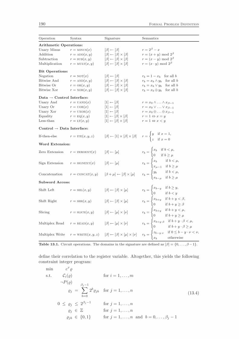
190 Formal Problem Definition
Operation Syntax Signature Semantics
Arithmetic Operations:
Unary Minus r = minus(x) [β]← [β] r = 2β − x
Addition r = add(x, y) [β]← [β]× [β] r = (x + y) mod 2β
Subtraction r = sub(x, y) [β]← [β]× [β] r = (x− y) mod 2β
Multiplication r = mult(x, y) [β]← [β]× [β] r = (x · y) mod 2β
Bit Operations:
Negation r = not(x) [β]← [β] rb = 1− xb for all b
Bitwise And r = and(x, y) [β]← [β]× [β] rb = xb ∧ yb for all b
Bitwise Or r = or(x, y) [β]← [β]× [β] rb = xb ∨ yb for all b
Bitwise Xor r = xor(x, y) [β]← [β]× [β] rb = xb⊕ yb for all b
Data → Control Interface:
Unary And r = uand(x) [1]← [β] r = x0 ∧ . . . ∧ xβ−1
Unary Or r = uor(x) [1]← [β] r = x0 ∨ . . . ∨ xβ−1
Unary Xor r = uxor(x) [1]← [β] r = x0⊕ . . .⊕xβ−1
Equality r = eq(x, y) [1]← [β]× [β] r = 1⇔ x = y
Less-than r = lt(x, y) [1]← [β]× [β] r = 1⇔ x < y
Control → Data Interface:
If-then-else r = ite(x, y, z) [β]← [1]× [β]× [β] r =
(
y if x = 1,
z if x = 0
Word Extension:
Zero Extension r = zeroext(x) [β]← [µ] rb =
(
xb if b < µ,
0 if b ≥ µ
Sign Extension r = signext(x) [β]← [µ] rb =
(
xb if b < µ,
xµ−1 if b ≥ µ
Concatenation r = concat(x, y) [β + µ]← [β]× [µ] rb =
(
yb if b < µ,
xb−µ if b ≥ µ
Subword Access:
Shift Left r = shl(x, y) [β]← [β]× [µ] rb =
(
xb−y if b ≥ y,
0 if b < y
Shift Right r = shr(x, y) [β]← [β]× [µ] rb =
(
xb+y if b + y < β,
0 if b + y ≥ β
Slicing r = slice(x, y) [β]← [µ]× [ν] rb =
(
xb+y if b + y < µ,
0 if b + y ≥ µ
Multiplex Read r = read(x, y) [β]← [µ]× [ν] rb =
(
xb+y·β if b + y · β < µ,
0 if b + y · β ≥ µ
Multiplex Write r = write(x, y, z) [β]← [β]× [µ]× [ν] rb =
(
zb−y·ν if 0 ≤ b− y · ν < ν,
xb otherwise
Table 13.1. Circuit operations. The domains in the signature are defined as [β] = {0, . . . , β−1}.
define their correlation to the register variable. Altogether, this yields the followingconstraint integer program:
min cT
s.t. Ci() for i = 1, . . . ,m
¬P ()
j =
βj−1∑
b=0
2bjb for j = 1, . . . , n
0 ≤ j ≤ 2βj−1 for j = 1, . . . , n
j ∈ Z for j = 1, . . . , n
jb ∈ {0, 1} for j = 1, . . . , n and b = 0, . . . , βj − 1
(13.4)
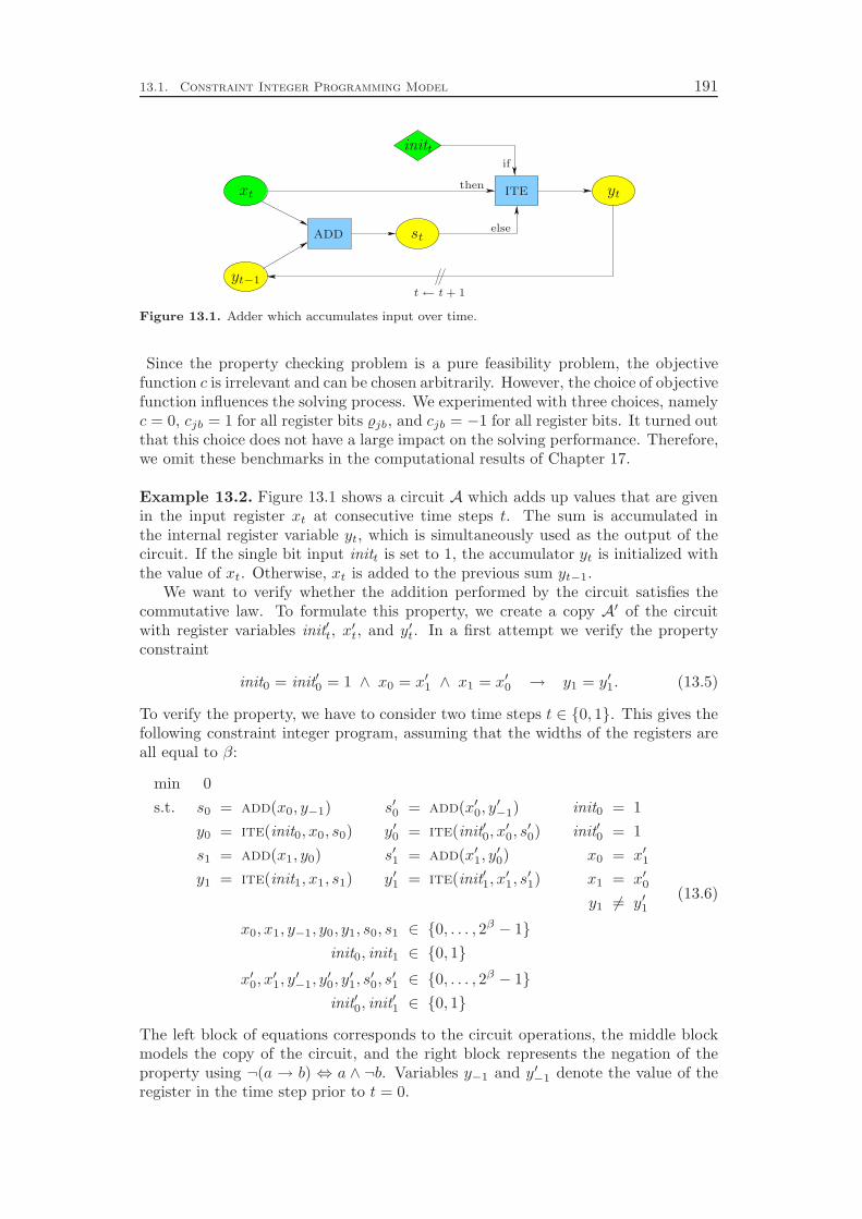
13.1. Constraint Integer Programming Model 191
xt
initt
yt−1
st
yt
add
ite
if
then
else
t← t + 1
Figure 13.1. Adder which accumulates input over time.
Since the property checking problem is a pure feasibility problem, the objectivefunction c is irrelevant and can be chosen arbitrarily. However, the choice of objectivefunction influences the solving process. We experimented with three choices, namelyc = 0, cjb = 1 for all register bits jb, and cjb = −1 for all register bits. It turned outthat this choice does not have a large impact on the solving performance. Therefore,we omit these benchmarks in the computational results of Chapter 17.
Example 13.2. Figure 13.1 shows a circuit A which adds up values that are givenin the input register xt at consecutive time steps t. The sum is accumulated inthe internal register variable yt, which is simultaneously used as the output of thecircuit. If the single bit input initt is set to 1, the accumulator yt is initialized withthe value of xt. Otherwise, xt is added to the previous sum yt−1.
We want to verify whether the addition performed by the circuit satisfies thecommutative law. To formulate this property, we create a copy A′ of the circuitwith register variables init′t, x
′t, and y′t. In a first attempt we verify the property
constraint
init0 = init′0 = 1 ∧ x0 = x′1 ∧ x1 = x′0 → y1 = y′1. (13.5)
To verify the property, we have to consider two time steps t ∈ {0, 1}. This gives thefollowing constraint integer program, assuming that the widths of the registers areall equal to β:
min 0
s.t. s0 = add(x0, y−1) s′0 = add(x′0, y′−1) init0 = 1
y0 = ite(init0, x0, s0) y′0 = ite(init′0, x′0, s′0) init′0 = 1
s1 = add(x1, y0) s′1 = add(x′1, y′0) x0 = x′1
y1 = ite(init1, x1, s1) y′1 = ite(init′1, x′1, s′1) x1 = x′0
y1 6= y′1
x0, x1, y−1, y0, y1, s0, s1 ∈ {0, . . . , 2β − 1}
init0, init1 ∈ {0, 1}
x′0, x′1, y′−1, y
′0, y′1, s′0, s′1 ∈ {0, . . . , 2
β − 1}
init′0, init′1 ∈ {0, 1}
(13.6)
The left block of equations corresponds to the circuit operations, the middle blockmodels the copy of the circuit, and the right block represents the negation of theproperty using ¬(a → b) ⇔ a ∧ ¬b. Variables y−1 and y′−1 denote the value of theregister in the time step prior to t = 0.

192 Formal Problem Definition
CIP (13.6) is feasible, for example with the input init0 = init′0 = init1 = init′1 = 1,x0 = x′1 = 0, and x1 = x′0 = 1, and the initial internal state y−1 = y′−1 = 0, whichyields the values s0 = y0 = 0, s1 = y1 = 1, s′0 = y′0 = s′1 = 1, and y′1 = 0 for theconstrained variables. This proves that the circuit violates Property (13.5). However,this does not necessarily mean that the circuit is flawed. In our case, the source ofthe error is the incorrect model of the property. To verify the commutativity law,we do not only have to fix init0 = init′0 = 1, but we also have to ensure that the initregister is 0 in the following time step. This yields the revised property
init0 = init′0 = 1 ∧ init1 = init′1 = 0 ∧ x0 = x′1 ∧ x1 = x′0 → y1 = y′1, (13.7)
which introduces the two additional fixings init1 = 0 and init′1 = 0 to System (13.6).The modified CIP is infeasible, which proves the validity of Property (13.7).
13.2 Function Graph
The circuit operations link up to three input registers x, y, and z to an outputregister r. The output is uniquely defined by the input, since the circuit operatorsare well-defined mappings. In every circuit, each register can be the output of atmost one operation. Registers that are not output of any operation are the inputregisters of the circuit, while the ones that are constrained by a circuit operationare internal or output registers. Therefore, the circuit as a whole is a well-definedmapping of input registers to internal and output registers.
This mapping can be represented as a function graph, which is a directed bipartitegraph G = (V ∪ VC, A) with two different types of nodes, namely register nodesV = {1, . . . , n} and constraint nodes VC = {C1, . . . , Cm}. The arc set is defined as
A = {(j , Ci) | register j is input of circuit operation Ci}
∪ {(Ci, j) | register j is output of circuit operation Ci}.
As the graph represents a chip design and therefore a well-defined mapping of inputsto outputs, it does not contain directed cycles.
If the input registers are fixed to certain values, the values of the internal and out-put registers can easily be calculated by forward propagation of the registers throughthe constraints, just like the chip would do in hardware. The property, however, mayrestrict the domains of internal and output registers, add other constraints, and canleave input registers unspecified. Therefore, an assignment of values to the unspeci-fied input registers may result in conflicting assignments for the internal and outputvariables.
Example 13.3. Figure 13.2 shows the function graph for the adder of Example 13.2including the invalid negated Property (13.5), which corresponds to the CIP (13.6).The left hand side part represents the time-expanded original circuit A, while theright hand side part represents the copy A′. The property is included by fixingthe input init0 in both circuits to init0 = init′0 = 1 and adding the constraints1 = eq(x0, x
′1), 1 = eq(x1, x
′0), and 0 = eq(y1, y
′1).
The function graph contains the complete structure of the circuit and the prop-erty. We use this concept in the irrelevance detection described in Section 15.2 to
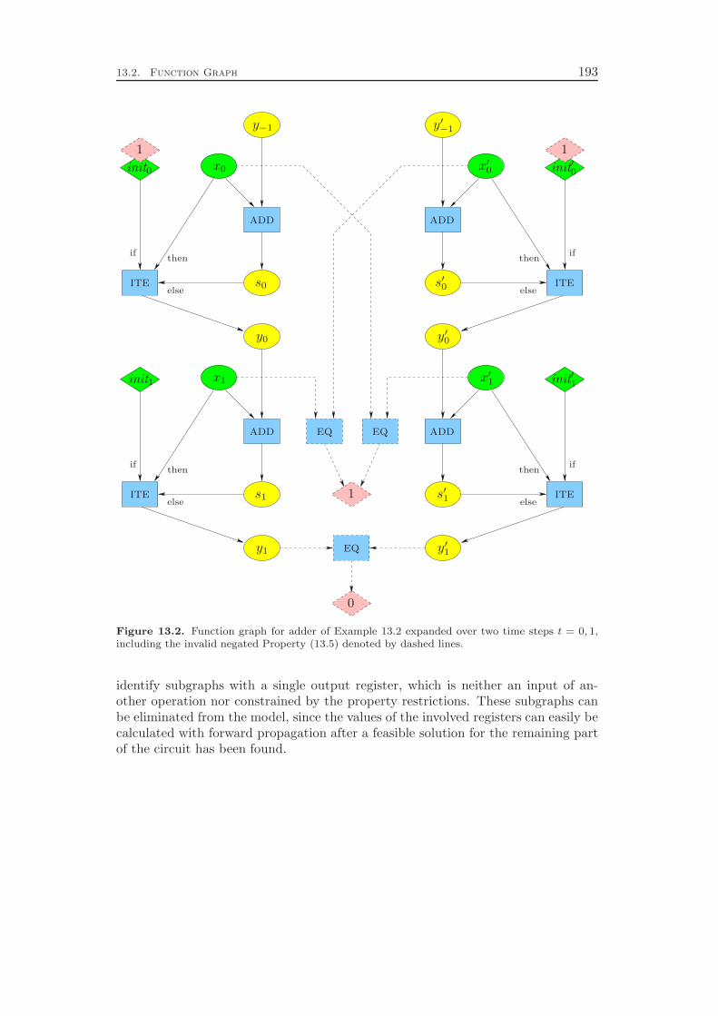
13.2. Function Graph 193
x′0 init′0
y′−1
s′0
y′0
x′1 init′1
s′1
y′1
x0init0
y−1
s0
y0
x1init1
s1
y1
0
11
1
add
addadd
add
ite
ite ite
ite
eq
eqeq
if if
ifif
then then
thenthen
else else
elseelse
Figure 13.2. Function graph for adder of Example 13.2 expanded over two time steps t = 0, 1,including the invalid negated Property (13.5) denoted by dashed lines.
identify subgraphs with a single output register, which is neither an input of an-other operation nor constrained by the property restrictions. These subgraphs canbe eliminated from the model, since the values of the involved registers can easily becalculated with forward propagation after a feasible solution for the remaining partof the circuit has been found.

Chapter 14
Operators in Detail
We solve the property checking CIP (13.4) with our branch-and-bound based con-straint integer programming framework SCIP. The problem instance is successivelydivided into subproblems by splitting the domains of the register variables into twodisjunctive parts: either by fixing a certain bit of a register to jb = 0 and jb = 1,respectively, or by introducing local upper bounds j ≤ v and local lower boundsj ≥ v + 1 on the individual registers.
At each node in the resulting search tree, we apply methods of constraint pro-gramming (Section 1.1), SAT solving (Section 1.2), and integer programming (Sec-tion 1.3) to tighten the local subproblem and to prune the search tree. Thisincludes domain propagation (Section 2.3), solving an LP relaxation with the op-tional possibility to add cutting planes (Section 2.2), and applying conflict analysis(Chapter 11) on infeasible subproblems.
The most important task in creating a SCIP application to solve a specific con-straint integer programming model is to implement the constraint handlers (seeSection 3.1.1) for the individual constraint classes that can appear in the model.
In our case of property checking, these are the circuit operator constraints ofTable 13.1 and the bit linking constraints (13.3). Each constraint handler definesthe semantics, constructs the LP relaxation, and provides domain propagation andreverse propagation algorithms for the constraint class for which it is responsible.Additionally, presolving algorithms specialized to the individual constraint classesreduce the complexity of the problem instance and detect inherent relations, whichcan be exploited during the solving process.
In the following, we will take a detailed look at the different circuit operatorsand describe the algorithms dealing with the corresponding constraints. For eachoperator, we present the linear equations and inequalities that are used to modelthe operator within the linear programming relaxation, and we describe the do-main propagation and presolving algorithms. The presentation is rather detailedand technical. It tries to convey the main algorithmic ideas to developers of chipdesign verification tools. For those who are not interested in the very details of thealgorithms, it suffices to read the introduction paragraphs of the individual circuitoperator sections in which we explain the main issues and difficulties associated withthe respective constraint class.
Table 14.1 gives a summary of the linear relaxations used for the circuit opera-tors. Very large coefficients like 2βr in the add linearization or in the bit linkingconstraints (13.3) can lead to numerical difficulties in the LP relaxation. Therefore,we split the register variables into words of W = 16 bits and apply the linearizationto the individual words. The linkage between the words is established in a properfashion. For example, the overflow bit of a word in an addition is added to the righthand side of the next word’s linearization (see Section 14.3.1). The partitioning ofregisters into words and bits is explained in detail in Section 14.1. The relaxationof the mult constraint involves additional variables y〈l〉 and r〈l〉 which are “nibbles”
195
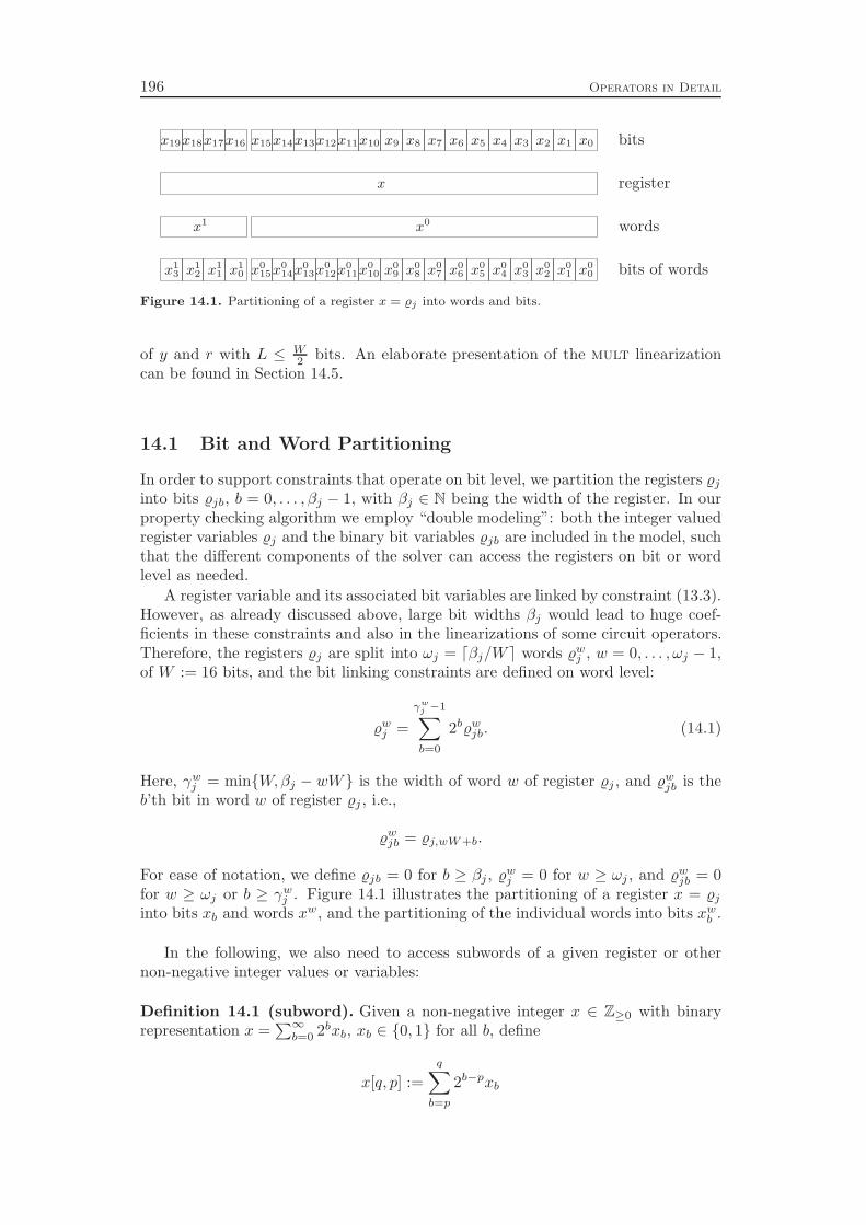
196 Operators in Detail
bits
register
words
bits of words
x19x18x17x16 x15x14x13x12x11x10 x9 x8 x7 x6 x5 x4 x3 x2 x1 x0
x
x0x1
x015x
014x
013x
012x
011x
010 x
09 x0
8 x07 x0
6 x05 x0
4 x03 x0
2 x01 x0
0x13 x1
2 x11 x1
0
Figure 14.1. Partitioning of a register x = j into words and bits.
of y and r with L ≤ W2
bits. An elaborate presentation of the mult linearizationcan be found in Section 14.5.
14.1 Bit and Word Partitioning
In order to support constraints that operate on bit level, we partition the registers j
into bits jb, b = 0, . . . , βj − 1, with βj ∈ N being the width of the register. In ourproperty checking algorithm we employ “double modeling”: both the integer valuedregister variables j and the binary bit variables jb are included in the model, suchthat the different components of the solver can access the registers on bit or wordlevel as needed.
A register variable and its associated bit variables are linked by constraint (13.3).However, as already discussed above, large bit widths βj would lead to huge coef-ficients in these constraints and also in the linearizations of some circuit operators.Therefore, the registers j are split into ωj = ⌈βj/W ⌉ words w
j , w = 0, . . . , ωj − 1,of W := 16 bits, and the bit linking constraints are defined on word level:
wj =
γwj −1∑
b=0
2bwjb. (14.1)
Here, γwj = min{W,βj − wW} is the width of word w of register j , and w
jb is theb’th bit in word w of register j , i.e.,
wjb = j,wW+b.
For ease of notation, we define jb = 0 for b ≥ βj , wj = 0 for w ≥ ωj , and w
jb = 0for w ≥ ωj or b ≥ γw
j . Figure 14.1 illustrates the partitioning of a register x = j
into bits xb and words xw, and the partitioning of the individual words into bits xwb .
In the following, we also need to access subwords of a given register or othernon-negative integer values or variables:
Definition 14.1 (subword). Given a non-negative integer x ∈ Z≥0 with binaryrepresentation x =
∑∞b=0 2bxb, xb ∈ {0, 1} for all b, define
x[q, p] :=
q∑
b=p
2b−pxb
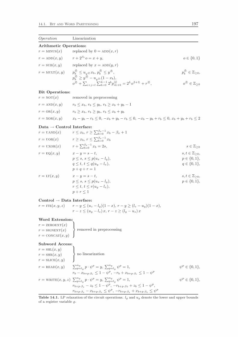
14.1. Bit and Word Partitioning 197
Operation Linearization
Arithmetic Operations:
r = minus(x) replaced by 0 = add(x, r)
r = add(x, y) r + 2βro = x+ y, o ∈ {0, 1}
r = sub(x, y) replaced by x = add(y, r)
r = mult(x, y) p〈l〉b ≤ uy〈l〉xb, p
〈l〉b ≤ y〈l〉, p
〈l〉b ∈ Z≥0,
p〈l〉b ≥ y〈l〉 − uy〈l〉(1 − xb),
o〈l〉 +P
i+j=l
PL−1
b=02bp
〈j〉iL+b = 2Lo〈l+1〉 + r〈l〉, o〈l〉 ∈ Z≥0
Bit Operations:
r = not(x) removed in preprocessing
r = and(x, y) rb ≤ xb, rb ≤ yb, rb ≥ xb + yb − 1
r = or(x, y) rb ≥ xb, rb ≥ yb, rb ≤ xb + yb
r = xor(x, y) xb − yb − rb ≤ 0, −xb + yb − rb ≤ 0, −xb − yb + rb ≤ 0, xb + yb + rb ≤ 2
Data → Control Interface:
r = uand(x) r ≤ xb, r ≥Pβx−1
b=0xb − βx + 1
r = uor(x) r ≥ xb, r ≤Pβx−1
b=0xb
r = uxor(x) r +Pβx−1
b=0xb = 2s, s ∈ Z≥0
r = eq(x, y) x− y = s− t, s, t ∈ Z≥0,
p ≤ s, s ≤ p(ux − ly), p ∈ {0, 1},
q ≤ t, t ≤ q(uy − lx), q ∈ {0, 1},
p+ q + r = 1
r = lt(x, y) x− y = s− t, s, t ∈ Z≥0,
p ≤ s, s ≤ p(ux − ly), p ∈ {0, 1},
r ≤ t, t ≤ r(uy − lx),
p+ r ≤ 1
Control → Data Interface:
r = ite(x, y, z) r − y ≤ (uz − ly)(1 − x), r − y ≥ (lz − uy)(1 − x),
r − z ≤ (uy − lz)x, r − z ≥ (ly − uz)x
Word Extension:
r = zeroext(x)
r = signext(x)
r = concat(x, y)
9
>
=
>
;
removed in preprocessing
Subword Access:
r = shl(x, y)
r = shr(x, y)
r = slice(x, y)
9
>
=
>
;
no linearization
r = read(x, y)Puy
p=lyp · ψp = y,
Puy
p=lyψp = 1, ψp ∈ {0, 1},
rb − xb+p·βr ≤ 1 − ψp, −rb + xb+p·βr ≤ 1 − ψp
r = write(x, y, z)Puy
p=lyp · ψp = y,
Puy
p=lyψp = 1, ψp ∈ {0, 1},
rb+p·βz − zb ≤ 1 − ψp, −rb+p·βz + zb ≤ 1 − ψp,
rb+p·βz − xb+p·βz ≤ ψp, −rb+p·βz + xb+p·βz ≤ ψp
Table 14.1. LP relaxation of the circuit operations. l and u denote the lower and upper boundsof a register variable .
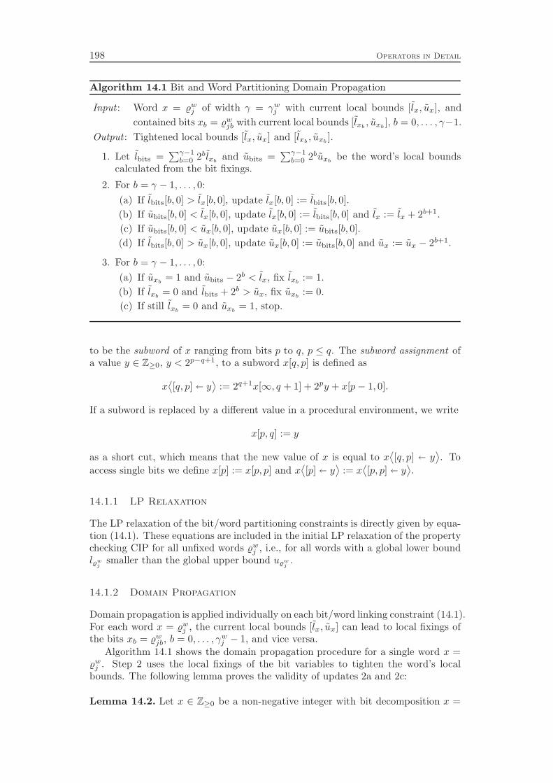
198 Operators in Detail
Algorithm 14.1 Bit and Word Partitioning Domain Propagation
Input : Word x = wj of width γ = γw
j with current local bounds [lx, ux], and
contained bits xb = wjb with current local bounds [lxb
, uxb], b = 0, . . . , γ−1.
Output : Tightened local bounds [lx, ux] and [lxb, uxb
].
1. Let lbits =∑γ−1
b=0 2blxband ubits =
∑γ−1b=0 2buxb
be the word’s local boundscalculated from the bit fixings.
2. For b = γ − 1, . . . , 0:
(a) If lbits[b, 0] > lx[b, 0], update lx[b, 0] := lbits[b, 0].
(b) If ubits[b, 0] < lx[b, 0], update lx[b, 0] := lbits[b, 0] and lx := lx + 2b+1.
(c) If ubits[b, 0] < ux[b, 0], update ux[b, 0] := ubits[b, 0].
(d) If lbits[b, 0] > ux[b, 0], update ux[b, 0] := ubits[b, 0] and ux := ux − 2b+1.
3. For b = γ − 1, . . . , 0:
(a) If uxb= 1 and ubits − 2b < lx, fix lxb
:= 1.
(b) If lxb= 0 and lbits + 2b > ux, fix uxb
:= 0.
(c) If still lxb= 0 and uxb
= 1, stop.
to be the subword of x ranging from bits p to q, p ≤ q. The subword assignment ofa value y ∈ Z≥0, y < 2p−q+1, to a subword x[q, p] is defined as
x⟨[q, p] � y
⟩:= 2q+1x[∞, q + 1] + 2py + x[p− 1, 0].
If a subword is replaced by a different value in a procedural environment, we write
x[p, q] := y
as a short cut, which means that the new value of x is equal to x⟨[q, p] � y
⟩. To
access single bits we define x[p] := x[p, p] and x⟨[p] � y
⟩:= x
⟨[p, p] � y
⟩.
14.1.1 LP Relaxation
The LP relaxation of the bit/word partitioning constraints is directly given by equa-tion (14.1). These equations are included in the initial LP relaxation of the propertychecking CIP for all unfixed words w
j , i.e., for all words with a global lower boundlw
jsmaller than the global upper bound uw
j.
14.1.2 Domain Propagation
Domain propagation is applied individually on each bit/word linking constraint (14.1).For each word x = w
j , the current local bounds [lx, ux] can lead to local fixings ofthe bits xb = w
jb, b = 0, . . . , γwj − 1, and vice versa.
Algorithm 14.1 shows the domain propagation procedure for a single word x =w
j . Step 2 uses the local fixings of the bit variables to tighten the word’s localbounds. The following lemma proves the validity of updates 2a and 2c:
Lemma 14.2. Let x ∈ Z≥0 be a non-negative integer with bit decomposition x =

14.1. Bit and Word Partitioning 199
∑∞b=0 2bxb. If lx ≤ x ≤ ux and lxb
≤ xb ≤ uxbfor all b, then
x ≥ lx⟨[b, 0] � lbits[b, 0]
⟩and x ≤ ux
⟨[b, 0] � ubits[b, 0]
⟩for all b ∈ Z≥0
with lbits =∑∞
b=0 2blxband ubits =
∑∞b=0 2buxb
being the integer values composedof the bounds for the bits of x.
Proof. We prove the case for the lower bound. Due to x ≥ lx it follows x[∞, b+1] ≥lx[∞, b + 1]. This leads to
x = 2bx[∞, b + 1] + x[b, 0]
≥ 2blx[∞, b+ 1] + lbits[b, 0]
= lx⟨[b, 0] � lbits[b, 0]
⟩.
The proof for the upper bound is analogous.
The reasoning in updates 2b and 2d is slightly different since they also includethe opposite bound:
Lemma 14.3. Let x ∈ Z≥0 be a non-negative integer with bit decomposition x =∑∞
b=0 2bxb. If lx ≤ x ≤ ux and lxb≤ xb ≤ uxb
for all b, then
ubits[b, 0] < lx[b, 0] ⇒ x ≥ lx⟨[b, 0] � lbits[b, 0]
⟩+ 2b+1
andlbits[b, 0] > ux[b, 0] ⇒ x ≤ ux
⟨[b, 0] � ubits[b, 0]
⟩− 2b+1
for all b ∈ Z≥0.
Proof. We prove the first implication. Let ubits[b, 0] < lx[b, 0] and assume x[∞, b +1] = lx[∞, b + 1]. From the bounds of the individual bits we know that x[b, 0] ≤ubits[b, 0]. Hence, x[b, 0] < lx[b, 0] which means x < lx, a contradiction. Therefore,x[∞, b + 1] > lx[∞, b+ 1], which means
x ≥ 2b+1(lx[∞, b+ 1] + 1
)= lx
⟨[b, 0] � 0
⟩+ 2b+1.
Lemma 14.2 yields
x ≥(lx⟨[b, 0] � 0
⟩+ 2b+1
)⟨[b, 0] � lbits[b, 0]
⟩
which is equivalent to
x ≥ lx⟨[b, 0] � lbits[b, 0]
⟩+ 2b+1
since the addition of 2b+1 does not influence the lower significant bits 0 to b. Theproof of the second implication is analogous.
The following lemma shows that changes made in iteration b = b′ of Step 2 donot enable further updates on the same or more significant bits b ≥ b′. Therefore,the loop of Step 2 only needs to be executed once.
Lemma 14.4. After Step 2 of Algorithm 14.1 was performed for all bits b > b′,subsequent bound changes deduced in Step 2 for bit b′ cannot enable additionaldeductions of the types of Step 2 for bits b ≥ b′.

200 Operators in Detail
Proof. Let b′ be the first (most significant) bit for which a deduction in Step 2 isperformed, and let lx ≤ x ≤ ux and lxb
≤ xb ≤ uxb, b = 0, . . . , γ − 1, be the bounds
before iteration b = b′ of Step 2 is executed. Then, we have lbits[b, 0] ≤ lx[b, 0] ≤ubits[b, 0] and lbits[b, 0] ≤ ux[b, 0] ≤ ubits[b, 0] for all b > b′, because no deductionswere applied for b > b′. It follows that also for the subwords up to bit b′+1 we have
lbits[b, b′ + 1] ≤ lx[b, b′ + 1] ≤ ubits[b, b
′ + 1] for all b > b′ (14.2)
andlbits[b, b
′ + 1] ≤ ux[b, b′ + 1] ≤ ubits[b, b′ + 1] for all b > b′.
A deduction for b = b′ in Step 2a fixes lx[b′, 0] := lbits[b′, 0]. This update has no
influence on deductions of type 2c and 2d, and due to (14.2), it also does not enableany further deductions of type 2a for bits b ≥ b′. If no infeasibility is detected, afterthe update we have lx[b, 0] = lbits[b, 0] ≤ ubits[b, 0] for all b ≤ b′, and again due to(14.2) no further deductions of type 2b are possible for b ≥ b′.
Now suppose that a deduction for b = b′ was applied in Step 2b. Again, theupdates on lx do not influence Steps 2c and 2d. If Step 2b can be applied at themost significant bit b′ = γ − 1, the constraint is proven to be infeasible. Therefore,it suffices to look at the case b′ < γ − 1.
At first, assume ubits[b′ + 1] ≤ lx[b′ + 1]. This implies that ubits[b
′ + 1, 0] <lx[b′ + 1, 0] would already have been satisfied in the previous iteration and Step 2bwould have been applied for bit b = b′+1. This contradicts the definition of b′ beingthe first iteration for which a deduction is performed. Therefore, the assumption iswrong and instead ubits[b
′ + 1] > lx[b′ + 1] must hold which gives ubits[b′ + 1] = 1
and lx[b′ + 1] = 0.It follows that even after adding 2b′+1 to lx, inequality (14.2) stays valid. Like
before, this shows that also the update of Step 2b cannot enable subsequent deduc-tions for b ≥ b′. With analogous reasoning it can be shown that also the updates ofSteps 2c and 2d do not trigger additional deductions for b ≥ b′. The case that b′ isnot the first iteration for which an update was applied follows by induction.
Corollary 14.5. After Step 2 of Algorithm 14.1 was performed completely, a secondrun of Step 2 would not produce any additional deductions. In particular, the boundssatisfy lbits[b, 0] ≤ lx[b, 0] ≤ ubits[b, 0] and lbits[b, 0] ≤ ux[b, 0] ≤ ubits[b, 0] for allb = 0, . . . , γ − 1.
In Step 3 of Algorithm 14.1 we check whether a fixing of a bit to a certain valuewould violate the word’s bounds, and in this case fix the bit to the opposite value.If a bit remains unfixed, no more less significant bits can be fixed with the reasoningof Steps 3a and 3b:
Lemma 14.6. If an unfixed bit xb was not fixed in Steps 3a or 3b of Algorithm 14.1,the conditions ubits − 2b′ < lx and lbits + 2b′ > ux do not hold for all less significantbits xb′ , b
′ < b.
Proof. First, suppose b′ is the most significant unfixed bit smaller than b. Since xb
was not fixed in Loop 3, we have lx ≤ ubits− 2b and ux ≥ lbits +2b. Because no newfixings have been found since bit xb was processed, lx, ux, lbits, and ubits were notchanged at the time xb′ is considered. It follows
ubits − 2b′ > ubits − 2b ≥ lx and lbits + 2b′ < lbits + 2b ≤ ux.
The case of an arbitrary position b′ < b follows by induction.
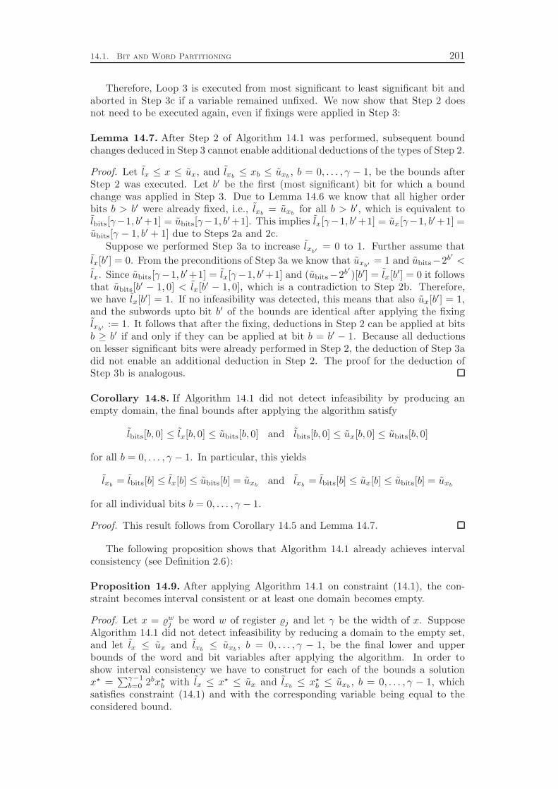
14.1. Bit and Word Partitioning 201
Therefore, Loop 3 is executed from most significant to least significant bit andaborted in Step 3c if a variable remained unfixed. We now show that Step 2 doesnot need to be executed again, even if fixings were applied in Step 3:
Lemma 14.7. After Step 2 of Algorithm 14.1 was performed, subsequent boundchanges deduced in Step 3 cannot enable additional deductions of the types of Step 2.
Proof. Let lx ≤ x ≤ ux, and lxb≤ xb ≤ uxb
, b = 0, . . . , γ − 1, be the bounds afterStep 2 was executed. Let b′ be the first (most significant) bit for which a boundchange was applied in Step 3. Due to Lemma 14.6 we know that all higher orderbits b > b′ were already fixed, i.e., lxb
= uxbfor all b > b′, which is equivalent to
lbits[γ−1, b′+1] = ubits[γ−1, b′+1]. This implies lx[γ−1, b′+1] = ux[γ−1, b′+1] =ubits[γ − 1, b′ + 1] due to Steps 2a and 2c.
Suppose we performed Step 3a to increase lxb′= 0 to 1. Further assume that
lx[b′] = 0. From the preconditions of Step 3a we know that uxb′= 1 and ubits−2b′ <
lx. Since ubits[γ−1, b′+1] = lx[γ−1, b′+1] and (ubits−2b′)[b′] = lx[b′] = 0 it followsthat ubits[b
′ − 1, 0] < lx[b′ − 1, 0], which is a contradiction to Step 2b. Therefore,we have lx[b′] = 1. If no infeasibility was detected, this means that also ux[b′] = 1,and the subwords upto bit b′ of the bounds are identical after applying the fixinglxb′
:= 1. It follows that after the fixing, deductions in Step 2 can be applied at bitsb ≥ b′ if and only if they can be applied at bit b = b′ − 1. Because all deductionson lesser significant bits were already performed in Step 2, the deduction of Step 3adid not enable an additional deduction in Step 2. The proof for the deduction ofStep 3b is analogous.
Corollary 14.8. If Algorithm 14.1 did not detect infeasibility by producing anempty domain, the final bounds after applying the algorithm satisfy
lbits[b, 0] ≤ lx[b, 0] ≤ ubits[b, 0] and lbits[b, 0] ≤ ux[b, 0] ≤ ubits[b, 0]
for all b = 0, . . . , γ − 1. In particular, this yields
lxb= lbits[b] ≤ lx[b] ≤ ubits[b] = uxb
and lxb= lbits[b] ≤ ux[b] ≤ ubits[b] = uxb
for all individual bits b = 0, . . . , γ − 1.
Proof. This result follows from Corollary 14.5 and Lemma 14.7.
The following proposition shows that Algorithm 14.1 already achieves intervalconsistency (see Definition 2.6):
Proposition 14.9. After applying Algorithm 14.1 on constraint (14.1), the con-straint becomes interval consistent or at least one domain becomes empty.
Proof. Let x = wj be word w of register j and let γ be the width of x. Suppose
Algorithm 14.1 did not detect infeasibility by reducing a domain to the empty set,and let lx ≤ ux and lxb
≤ uxb, b = 0, . . . , γ − 1, be the final lower and upper
bounds of the word and bit variables after applying the algorithm. In order toshow interval consistency we have to construct for each of the bounds a solutionx⋆ =
∑γ−1b=0 2bx⋆
b with lx ≤ x⋆ ≤ ux and lxb≤ x⋆
b ≤ uxb, b = 0, . . . , γ − 1, which
satisfies constraint (14.1) and with the corresponding variable being equal to theconsidered bound.
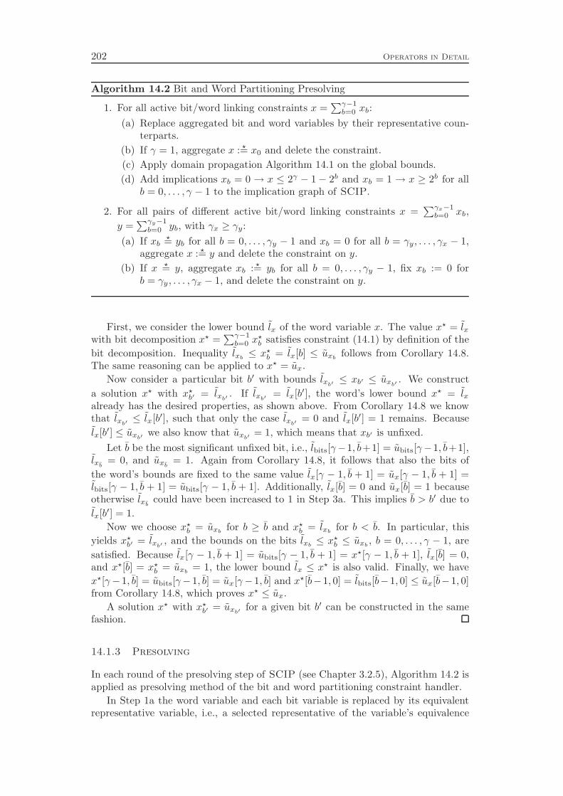
202 Operators in Detail
Algorithm 14.2 Bit and Word Partitioning Presolving
1. For all active bit/word linking constraints x =∑γ−1
b=0 xb:
(a) Replace aggregated bit and word variables by their representative coun-terparts.
(b) If γ = 1, aggregate x : ⋆= x0 and delete the constraint.
(c) Apply domain propagation Algorithm 14.1 on the global bounds.
(d) Add implications xb = 0 → x ≤ 2γ − 1− 2b and xb = 1 → x ≥ 2b for allb = 0, . . . , γ − 1 to the implication graph of SCIP.
2. For all pairs of different active bit/word linking constraints x =∑γx−1
b=0 xb,
y =∑γy−1
b=0 yb, with γx ≥ γy:
(a) If xb⋆= yb for all b = 0, . . . , γy − 1 and xb = 0 for all b = γy, . . . , γx − 1,
aggregate x : ⋆= y and delete the constraint on y.
(b) If x ⋆= y, aggregate xb : ⋆= yb for all b = 0, . . . , γy − 1, fix xb := 0 forb = γy , . . . , γx − 1, and delete the constraint on y.
First, we consider the lower bound lx of the word variable x. The value x⋆ = lxwith bit decomposition x⋆ =
∑γ−1b=0 x
⋆b satisfies constraint (14.1) by definition of the
bit decomposition. Inequality lxb≤ x⋆
b = lx[b] ≤ uxbfollows from Corollary 14.8.
The same reasoning can be applied to x⋆ = ux.
Now consider a particular bit b′ with bounds lxb′≤ xb′ ≤ uxb′
. We construct
a solution x⋆ with x⋆b′ = lxb′
. If lxb′= lx[b′], the word’s lower bound x⋆ = lx
already has the desired properties, as shown above. From Corollary 14.8 we knowthat lxb′
≤ lx[b′], such that only the case lxb′= 0 and lx[b′] = 1 remains. Because
lx[b′] ≤ uxb′we also know that uxb′
= 1, which means that xb′ is unfixed.
Let b be the most significant unfixed bit, i.e., lbits[γ−1, b+1] = ubits[γ−1, b+1],lxb
= 0, and uxb= 1. Again from Corollary 14.8, it follows that also the bits of
the word’s bounds are fixed to the same value lx[γ − 1, b + 1] = ux[γ − 1, b + 1] =lbits[γ − 1, b + 1] = ubits[γ − 1, b + 1]. Additionally, lx[b] = 0 and ux[b] = 1 becauseotherwise lxb
could have been increased to 1 in Step 3a. This implies b > b′ due to
lx[b′] = 1.
Now we choose x⋆b = uxb
for b ≥ b and x⋆b = lxb
for b < b. In particular, this
yields x⋆b′ = lxb′
, and the bounds on the bits lxb≤ x⋆
b ≤ uxb, b = 0, . . . , γ − 1, are
satisfied. Because lx[γ − 1, b + 1] = ubits[γ − 1, b + 1] = x⋆[γ − 1, b + 1], lx[b] = 0,and x⋆[b] = x⋆
b = uxb= 1, the lower bound lx ≤ x⋆ is also valid. Finally, we have
x⋆[γ−1, b] = ubits[γ−1, b] = ux[γ−1, b] and x⋆[b−1, 0] = lbits[b−1, 0] ≤ ux[b−1, 0]from Corollary 14.8, which proves x⋆ ≤ ux.
A solution x⋆ with x⋆b′ = uxb′
for a given bit b′ can be constructed in the samefashion.
14.1.3 Presolving
In each round of the presolving step of SCIP (see Chapter 3.2.5), Algorithm 14.2 isapplied as presolving method of the bit and word partitioning constraint handler.
In Step 1a the word variable and each bit variable is replaced by its equivalentrepresentative variable, i.e., a selected representative of the variable’s equivalence
14.1. Bit and Word Partitioning 203
class, see Section 3.3.4. Thereby, the constraint is normalized and two equivalentconstraints would contain exactly the same variables. This property is needed for afast equivalence detection in Step 2.
If the word consists of only one bit, the word variable x is equivalent to the bitvariable x0 and they are aggregated in Step 1b. Thereby, the equivalence classes ofx and x0 are implicitly united, see again Section 3.3.4. Since after the aggregation,the constraint x = x0 is always valid, we can delete the constraint from the problemformulation.
Step 1c calls Algorithm 14.1 as a subroutine to perform domain propagationon the global bounds. Afterwards, we enrich the implication graph of SCIP (seeSection 3.3.5) with the deductions on the word variable if a single bit is fixed to acertain value.
In Step 2 all pairs of bit/word linking constraints are processed. If all bitvariables (counting non-existing ones as being fixed to zero) of the two constraintsare equivalent, the word variables can be aggregated since they are also equivalent.If on the other hand the word variables are equivalent, the individual pairs of bitvariables can be aggregated, and the excessive bit variables of the wider word can befixed to zero. In both cases, one of the constraints can be deleted from the problemformulation.
14.1.4 Equivalence of Registers
Within the framework of constraint integer programming, the bit/word linking con-straints (14.1) are just ordinary constraints without any special meaning. In thechip verification application, these constraints are tightly connected to the abstractobjects of registers. Although being constraints in the CIP context, the registersappear as variables in the definitions of the circuit operations.
Like ordinary CIP variables, registers can be equivalent to each other, therebyforming equivalence classes with each of them being represented by a unique repre-sentative, see Section 3.3.4.
Definition 14.10 (equivalence of registers). We call two registers i and j
equivalent if the binary variables in their respective bit decomposition are pairwiseequivalent:
i⋆= j ⇔ ∀b ∈ Z≥0 : ib
⋆= jb (14.3)
with ib = 0 if b ≥ βi and jb = 0 if b ≥ βj . In an algorithmic environment, wedenote by
i :⋆= j ⇔ ∀b ∈ Z≥0 : ib :
⋆= jb
the aggregation of register i to j , which means to aggregate the individual pairsof binary variables in the bit decompositions of the registers.
For example, if we already know that y = 0, the addition constraint r = add(x, y)would detect that r and x are equivalent, which means that the individual word andbit variables of r = i are equivalent to their respective counterparts of x = j .Besides aggregating x : ⋆= r, we could in principle also identify the two register nodesx and r in the function graph, see Section 13.2, and replace all occurrences of x byr in the circuit constraints of the problem instance. Nevertheless, the identificationof register nodes in the function graph can destroy the structure of the graph. Forexample, if two output registers are identified, the two operations producing these

204 Operators in Detail
outputs receive an artificial connection through the unified output register that didnot exist in the original function graph. Consequently, loose ends of the graph,which are identified by the irrelevance detection of Section 15.2, may get lost, andthe performance of the presolving deteriorates. For this reason, we do not replaceregisters with the representative of their equivalence class in the circuit constraintsand in the function graph. Instead, equivalence of registers is always tested bychecking the individual bits for pairwise equivalence.
Just like detecting equivalences between registers it might happen that the globalinequality of two registers x and y is discovered. For example, if the constraintr = eq(x, y) is included in the problem and we know already that r = 0, we canconclude that x and y can never take the same value. We denote this fact by writingx Y
⋆= y:
Definition 14.11 (inequality of registers). We call two registers i and j un-equal if for each feasible solution of the property checking CIP (13.4) there is at leastone pair of binary variables in the bit decomposition of the registers with oppositevalues:
i Y⋆= j ⇔ ∀⋆ : C(⋆) ∧ ¬P (⋆) ∃b ∈ Z≥0 : ⋆
ib 6= ⋆jb (14.4)
with ⋆ib = 0 if b ≥ βi and ⋆
jb = 0 if b ≥ βj .
For each register x we store the set of registers y with x Y⋆= y as a sorted list
on which a binary search can be performed. Note that for two registers x and y itmay neither x ⋆= y nor x Y
⋆= y, since Y
⋆= is not the negated relation of ⋆=. However,
x ⋆= y ∧ x Y⋆= y proves the infeasibility of the problem instance.
14.2 Unary Minus
The unary minus operator
minus : [β]→ [β], x 7→ r = minus(x)
calculates the two’s complement of input register x, which is defined as
r = minus(x) ⇔ r = 2β − x.
This is equivalent to r+x = 2β, and due to the truncation of the overflow in the addoperand, the constraint can be represented as 0 = add(x, r). This transformationis applied in the presolving stage of SCIP, such that we do not need to implementany specific algorithms for the minus operator.
14.3 Addition
The two’s complement addition of two numbers x, y ∈ {0, . . . , 2β − 1} is defined as
add : [β]× [β]→ [β], (x, y) 7→ r = add(x, y)
withr = add(x, y) ⇔ r = (x+ y) mod 2β.
14.3. Addition 205
To overcome the numerical difficulties caused by very large coefficients, the LPrelaxation of addition constraints is defined on word level. Each word addition pro-duces an overflow that is passed to the next word’s calculations. The final overflowis ignored, which models the modulus operation in the above definition of the addoperator.
The domain propagation is applied on bit level and exploits knowledge aboutfixings and equivalences of the involved register bits. The word level and bit levelrepresentations interact by means of the bit/word linking constraints (14.1). Pre-solving operates on both representations simultaneously. In addition to the domainpropagation, it exploits global knowledge of equality or inequality of registers totighten the bounds of the bit and word variables. It also compares pairs of addconstraints to detect further problem simplifications.
14.3.1 LP Relaxation
Since for the input registers we have x, y ≤ 2β − 1, we know that the sum x + y isbounded by x + y ≤ 2β. Therefore, the sum can be completely described by β + 1bits, and the addition operand add just means to strip the most significant bit,called overflow bit, from the result. The LP relaxation of the constraint could bestated as
x+ y = r + 2βo with o ∈ {0, 1}, (14.5)
but for large bit widths β this would lead to numerical difficulties in the floating pointcalculations. The default parameter value for the feasibility tolerance for floatingpoint operations in SCIP is δ = 10−6. This value is also used for solving the LPrelaxations. Equality of floating point numbers in this sense is defined as
x.= y ⇔
|x− y|
max{|x|, |y|, 1}≤ δ. (14.6)
This means, for example, that for β = 20, x = y = 219, r = 1, and o = 1 we havex+ y = 220 6= 220 + 1 = r + 220o, but x+ y
.= r + 220o because
|220 − (220 + 1)|
max{|220|, |220 + 1|, 1}=
1
220 + 1≈ 9.5 · 10−7 < δ = 10−6.
Therefore, the invalid solution 1 = add(219, 219) would be accepted as feasible bythe LP solver.
In order to avoid these numerical difficulties, we restrict the coefficients in thelinear relaxation (14.5) to be not larger than 216, which can be achieved by splittingthe registers into words of W = 16 bits, as described in Section 14.1. For each wordw = 0, . . . , ω− 1, ω = ⌈β/W ⌉, of width γw = min{W,β−wW} we add the equation
xw + yw + ow = rw + 2γw
ow+1 with ow, ow+1 ∈ {0, 1} (14.7)
to the LP relaxation. Here, the overflow for a word is passed to the left hand sideof the next word’s equation. Note that the least significant overflow is fixed toow = 0. The system of equations (14.7) for all words w together with the bit/wordlinking constraints (14.1) is equivalent to equation (14.5) but rules out invalid integer
solutions even if the floating point equality (14.6) with feasibility tolerance δ = 10−6
is applied.

206 Operators in Detail
+
=
x18x17x16 x15x14x13x12x11x10 x9 x8 x7 x6 x5 x4 x3 x2 x1 x0
y18 y17 y16 y15 y14 y13 y12 y11 y10 y9 y8 y7 y6 y5 y4 y3 y2 y1 y0
o19 o18 o17 o16 o15 o14 o13 o12 o11 o10 o9 o8 o7 o6 o5 o4 o3 o2 o1 o0
r18 r17 r16 r15 r14 r13 r12 r11 r10 r9 r8 r7 r6 r5 r4 r3 r2 r1 r0
first input
second input
overflow
resultant
Figure 14.2. Bit level addition scheme.
14.3.2 Domain Propagation
Domain propagation for the addition operand is applied on bit level using the usualbit level addition scheme depicted in Figure 14.2. For each bit b = 0, . . . , β − 1 wepropagate the equation
xb + yb + ob = rb + 2ob+1. (14.8)
Note that o0 = 0, since there is no overflow passed to the least significant column.Observe also that the overflow ow of a word w in the LP relaxation (14.7) is alwaysequal to the bit overflow owW at the word boundary because wordwise addition andbitwise addition are equivalent, which can be seen by adding up equations (14.8) fora word w ∈ {0, . . . , ω − 1} of width γw:
xwW+0 + ywW+0 + 20owW+0 = rwW+0 + 2owW+1
∣∣ · 20
. . .
xwW+γw−1 + ywW+γw−1 + owW+γw−1 = rwW+γw−1 + 2owW+γw
∣∣ · 2γw−1
xw + yw +
γw−1∑
b=0
2bowW+b = rw +
γw
∑
b=1
2bowW+b
which is equivalent to
xw + yw + owW = rw + 2γw
owW+γw .
Subtracting equation (14.7) yields
owW − ow = 2γw
(owW+γw − ow+1),
and since the variables are binary and γw ≥ 1, it follows ow = owW and ow+1 =owW+γw . Thus, we can aggregate
ow :⋆= owW for all words w = 0, . . . , ω − 1, (14.9)
andoω :
⋆= oβ (14.10)
for the most significant overflow.Algorithm 14.3 illustrates the domain propagation method applied to add con-
straints. In fact, the deductions performed in Step 1 are just the usual boundtightening operations for the linear constraint (14.8), and the deductions of Step 2are equal to the ones for the linear constraint (14.7), see Section 7.1.
14.3. Addition 207
Algorithm 14.3 Addition Domain Propagation
Input : Addition constraint r = add(x, y) on registers r, x, and y of width βwith current local word bounds lrw ≤ rw ≤ urw , lxw ≤ xw ≤ uxw , andlyw ≤ yw ≤ uyw , and bit bounds lrb
≤ rb ≤ urb, lxb
≤ xb ≤ uxb, and
lyb≤ yb ≤ uyb
.
Output : Tightened local bounds for words rw, xw, yw, and bits rb, xb, yb.
1. For b = 0, . . . , β − 1:
(a) If three out of the four variables xb, yb, ob, and rb in the addition columnb are fixed, the fourth variable and the overflow ob+1 can be deduced byinspecting equation (14.8).
(b) If uxb+ uyb
+ uob− lrb
≤ 1, deduce ob+1 = 0.
(c) If lxb+ lyb
+ lob− urb
≥ 1, deduce ob+1 = 1.
(d) If uob+1= 0 and urb
= 0, deduce xb = yb = ob = 0.
(e) If lob+1= 1 and lrb
= 1, deduce xb = yb = ob = 1.
(f) If uob+1= 0 and one out of the three variables xb, yb, ob is fixed to one,
we can fix rb = 1 and the other two variables can be deduced to zero.
(g) If lob+1= 1 and one out of the three variables xb, yb, ob is fixed to zero,
we can fix rb = 0 and the other two variables can be deduced to one.
2. For w = 0, . . . , ω − 1: If ow+1 is fixed, deduce
lrw − uyw − uow + 2γw
ow+1 ≤ xw ≤ urw − lyw − low + 2γw
ow+1
lrw − uxw − uow + 2γw
ow+1 ≤ yw ≤ urw − lxw − low + 2γw
ow+1
lxw + lyw + low − 2γw
ow+1 ≤ rw ≤ uxw + uyw + uow − 2γw
ow+1
Because the word overflow variables ow are aggregated with the bit overflow vari-ables at the word boundaries, see (14.9) and (14.10), the propagations on the twoequations (14.8) and (14.7) can interact with each other. Additionally, the propa-gations on the overflow bits of Step 1 can influence the previous and next columnin the addition scheme of Figure 14.2. Furthermore, fixings of the bits and tight-enings of the words’ bounds can lead to even more implications in the propagationAlgorithm 14.1 for the bit/word linking constraints (14.1). SCIP exploits theseinterdependencies automatically by iteratively calling the individual domain prop-agation algorithms as long as additional deductions were found, see Section 3.1.4.Therefore, we can refrain from iterating Steps 1 and 2 inside Algorithm 14.3.
14.3.3 Presolving
In the presolving stage of SCIP, Algorithm 14.4 is executed to process the activeaddition constraints. Step 1a checks whether one of the two operands x and yis fixed to zero, which means that the resultant can be aggregated with the otheroperand. If on the other hand, one of the operands is proven to be non-zero, theresultant cannot be equal to the other operand and the sets of unequal registersfor the resultant and the other operand can be extended in Step 1b. Consequently,we can fix an operand to zero in Step 1c whenever the resultant is detected to be

208 Operators in Detail
Algorithm 14.4 Addition Presolving
1. For all active addition constraints r = add(x, y):
(a) If x = 0, aggregate r : ⋆= y and delete the constraint.If y = 0, aggregate r : ⋆= x and delete the constraint.
(b) If lxw ≥ 1 for any word w, deduce r Y⋆= y.
If lyw ≥ 1 for any word w, deduce r Y⋆= x.
(c) If r ⋆= x, fix y := 0 and delete the constraint.If r ⋆= y, fix x := 0 and delete the constraint.
(d) If r Y⋆= x and ωy = 1, deduce y0 ≥ 1.
If r Y⋆= y and ωx = 1, deduce x0 ≥ 1.
(e) If x ⋆= y, replace the constraint by r = shl(x, 1).
(f) If β = 1, replace the constraint by r = xor(x, y).
(g) Apply domain propagation Algorithm 14.3 on the global bounds.
(h) If two of the binary variables in equation (14.8) are equivalent or negatedequivalent, the others can be aggregated as shown in Algorithm 14.5.
(i) Add implications on binary variables using Algorithm 14.6.
2. For all pairs of active addition constraints r = add(x, y) and r′ = add(x′, y′)with βr ≥ βr′ :
(a) For all b = 0, . . . , βr′ :If (χb, ψb, φb) and (χ′b, ψ
′b, φ′b) are permutations of (xb, yb, ob) and
(x′b, y′b, o′b) such that χb
⋆= χ′b and ψb⋆= ψ′b, and
i. if φb⋆= φ′b, aggregate rb : ⋆= r′b and ob+1 : ⋆= o′b+1,
ii. if rb⋆= r′b, aggregate φb : ⋆= φ′b and ob+1 : ⋆= o′b+1,
iii. if rb Y⋆= r′b or ob+1 Y
⋆= o′b+1, aggregate φb : ⋆= 1− φ′b,
iv. if φb Y⋆= φ′b or ob+1 Y
⋆= o′b+1, aggregate rb : ⋆= 1− r′b.
(b) If Steps 2(a)i or 2(a)ii were successfully applied to all bits b = 0, . . . , βr′ ,delete constraint r′ = add(x′, y′).
(c) If βr = βr′ , x ⋆= x′, but r Y⋆= r′, deduce y Y
⋆= y′.
If βr = βr′ , y ⋆= y′, but r Y⋆= r′, deduce x Y
⋆= x′.
(d) If βr = βr′ , x ⋆= y′, but r Y⋆= r′, deduce y Y
⋆= x′.
If βr = βr′ , y ⋆= x′, but r Y⋆= r′, deduce x Y
⋆= y′.
always equal to the other operand. Step 1d deals with the backward implication ofStep 1a. If we know that the resultant is always unequal to one of the operands, wecan conclude that the other operand cannot be zero. However, it is impossible toexpress an inequality like y ≥ 1 for a register y in terms of bounds of CIP variables,since registers represent a collection of bit and word variables. We can only concludethat at least one of the words and one of the bits must be non-zero. Therefore, weare only able to deduce a bound change, if the register consists of a single word, i.e.,ω = 1.
In the case that the two operands are always equal, we can replace the addconstraint in Step 1e by an shl constraint, because add(x, x) = mult(x, 2) =shl(x, 1) for all x ∈ Z≥0. Of course, the presolving algorithm for the shl constraintwith the second operand fixed to one aggregates the bits to r0 := 0 and rb : ⋆= xb−1
14.3. Addition 209
Algorithm 14.5 Addition Presolving – Bit Aggregation
Considering equation (14.8), we can apply the following aggregations:
1. If xb⋆= yb aggregate ob : ⋆= rb and ob+1 : ⋆= xb.
2. If xb Y⋆= yb aggregate ob : ⋆= 1− rb and ob+1 : ⋆= ob.
3. If xb⋆= ob aggregate yb : ⋆= rb and ob+1 : ⋆= xb.
4. If xb Y⋆= ob aggregate yb : ⋆= 1− rb and ob+1 : ⋆= yb.
5. If xb⋆= rb aggregate ob : ⋆= yb and ob+1 : ⋆= yb.
6. If xb Y⋆= rb aggregate ob : ⋆= 1− yb and ob+1 : ⋆= xb.
7. If yb⋆= ob aggregate xb : ⋆= rb and ob+1 : ⋆= yb.
8. If yb Y⋆= ob aggregate xb : ⋆= 1− rb and ob+1 : ⋆= xb.
9. If yb⋆= rb aggregate ob : ⋆= xb and ob+1 : ⋆= xb.
10. If yb Y⋆= rb aggregate ob : ⋆= 1− xb and ob+1 : ⋆= yb.
11. If ob⋆= rb aggregate xb : ⋆= yb and ob+1 : ⋆= yb.
12. If ob Y⋆= rb aggregate xb : ⋆= 1− yb and ob+1 : ⋆= ob.
13. If xb Y⋆= ob+1 aggregate yb : ⋆= ob+1, ob : ⋆= ob+1, and rb : ⋆= xb.
14. If yb Y⋆= ob+1 aggregate xb : ⋆= ob+1, ob : ⋆= ob+1, and rb : ⋆= yb.
15. If ob Y⋆= ob+1 aggregate xb : ⋆= ob+1, yb : ⋆= ob+1, and rb : ⋆= ob.
16. If rb⋆= ob+1 aggregate xb : ⋆= rb, yb : ⋆= rb, and ob : ⋆= rb.
for b = 1, . . . , βr − 1, see Step 1e of Algorithm 14.28.In the very special case that the registers are single bits, i.e., β = 1, truncated
addition is equivalent to exclusive or, such that the constraint r = add(x, y) can bereplaced by r = xor(x, y) in Step 1f. The bitwise exclusive or constraint describedin Section 14.9 comes with a stronger LP relaxation than equation (14.5) becausethe introduction of the auxiliary binary overflow variable o can be avoided.
It may happen that two of the bit variables in equation (14.8) are equivalentor negated equivalent. The latter means that the two bits always take oppositevalues. For each bit b, there are
(52
)= 10 different pairs out of the five variables
involved in equation (14.8), which gives 20 combinations of potential equivalent ornegated equivalent binary variables. We can draw useful conclusions from 16 ofthese relationships, as shown in Algorithm 14.5. For the remaining four, namelyxb
⋆= ob+1, yb⋆= ob+1, ob
⋆= ob+1, and rb Y⋆= ob+1, we cannot deduce any further
equivalence or negated equivalence relations between two variables. For example, ifxb
⋆= ob+1, there are still the six solutions
(xb, yb, ob, rb, ob+1) ∈{(0, 0, 0, 0, 0), (0, 1, 0, 1, 0), (0, 0, 1, 1, 0),
(1, 1, 0, 0, 1), (1, 0, 1, 0, 1), (1, 1, 1, 1, 1)}
possible, and none of yb⋆= ob, yb
⋆= rb, ob⋆= rb, yb Y
⋆= ob, yb Y
⋆= rb, and ob Y
⋆= rb holds.
Note that Algorithm 14.5 would also find the fixings and aggregations of Steps 1aand 1c of Algorithm 14.4. Thus, the only additional value of those steps is thedeletion of the constraint.
The final task for each bit b in Loop 1 of Algorithm 14.4 is to add implicationsto the implication graph of SCIP, see Section 3.3.5. Algorithm 14.6 subsumes the
210 Operators in Detail
Algorithm 14.6 Addition Presolving – Implications
Considering equation (14.8), we can add the following implications to the implicationgraph of SCIP:
1. If xb = 0, add yb = 0→ ob+1 = 0 and ob = 0→ ob+1 = 0.
2. If xb = 1, add yb = 1→ ob+1 = 1 and ob = 1→ ob+1 = 1.
3. If yb = 0, add xb = 0→ ob+1 = 0 and ob = 0→ ob+1 = 0.
4. If yb = 1, add xb = 1→ ob+1 = 1 and ob = 1→ ob+1 = 1.
5. If ob = 0, add xb = 0→ ob+1 = 0 and yb = 0→ ob+1 = 0.
6. If ob = 1, add xb = 1→ ob+1 = 1 and yb = 1→ ob+1 = 1.
7. If ob+1 = 0, add xb = 1→ yb = 0, xb = 1→ ob = 0, and yb = 1→ ob = 0.
8. If ob+1 = 1, add xb = 0→ yb = 1 and xb = 0→ ob = 1, and yb = 0→ ob = 1.
implications that we can generate for each addition column, given that a certain bitin the column is already fixed.
Step 2 of Algorithm 14.4 compares all pairs of active addition constraints r =add(x, y) and r′ = add(x′, y′). Suppose two of the variables in {xb, yb, ob} arepairwise equivalent to two of {x′b, y
′b, o′b}. We call the remaining variables φb and φ′b,
respectively. Then, subtracting the bit equations (14.8) from each other yields
φb − φ′b = rb − r
′b + 2(ob+1 − o
′b+1).
Since all involved variables are binary, we can deduce the aggregations of Steps 2(a)ito 2(a)iv. Note that 2(a)iii and 2(a)iv are just the inverse implications of 2(a)iand 2(a)ii. If the equivalence of the bit equations (14.8) is detected for all bitsb = 0, . . . , βr′ by successful applications of Rules 2(a)i or 2(a)ii, the constraint onthe smaller or equally wide registers can be deleted in Step 2b, since its semanticsis already captured by the other constraint.
The trivial implications
βr ≥ βr′ ∧ (x⋆= x′) ∧ (y
⋆= y′) → r[βr′ − 1, 0]
⋆= r′ and
βr ≥ βr′ ∧ (x⋆= y′) ∧ (y
⋆= x′) → r[βr′ − 1, 0]
⋆= r′
are already covered by Step 2a. Steps 2c and 2d apply these implications in theopposite direction to deduce inequalities of operands. Note that we can only concludethat the operands are unequal if the resultants are of equal width. Otherwise, theinequality of the resultants may result from the different truncation of the sum. Analternative approach would be to check whether r[βr′ − 1, 0] Y
⋆= r′, but we do not
store inequalities between subwords of registers in our data structures.
14.4 Subtraction
The subtraction operator
sub : [β]× [β]→ [β], (x, y) 7→ r = sub(x, y)
yields the difference of the two input registers x and y in the two’s complementrepresentation. It is defined as
r = sub(x, y) ⇔ r = (x− y) mod 2β.
14.5. Multiplication 211
Because the integers modulo 2β together with the truncated addition and multipli-cation form a ring, we have x = (r + y) mod 2β. Therefore, we can replace eachsubtraction constraint by an equivalent addition constraint, which is performed inthe presolving stage of SCIP.
14.5 Multiplication
The multiplication operator
mult : [β]× [β]→ [β], (x, y) 7→ r = mult(x, y)
with
r = mult(x, y) ⇔ r = (x · y) mod 2β
is the most complex operator in terms of the algorithms involved to process the con-straints. Our implementation contains more than 7000 lines of C source code, whilethe implementation of the algorithms for addition, which is the second largest code,consists of only around 3500 lines. This corresponds to the observation, that SATand BDD based techniques often fail on circuits that involve lots of multiplications,which can also be seen in the computational results of Chapter 17.
The LP relaxation of multiplication constraints is quite involved. Like in writtenmultiplication learned in school, we multiply each digit of one operand by the digits ofthe other operand and align the results with respect to the significance of the involveddigits. Afterwards, these partial products are added up to yield the resultant of themultiplication constraint. Since a multiplication of two variables is a non-linearoperation, we cannot use it directly inside a linear relaxation. However, a productof a binary variable with another variable can be linearized by three inequalities.Therefore, the “digits” of one of the operands are given by its bit decomposition,while for the “digits” of the other operand we use half-words, so called nibbles.This asymmetric treatment of the two operands in a commutative operation raisesthe question which operand should be split into bits and which should be splitinto nibbles. This question is addressed in the presolving algorithm explained inSection 14.5.3.
We employ three different types of domain propagation algorithms for multconstraints. The first operates on the multiplication table of the LP relaxation andthe involved auxiliary variables, namely the partial products and overflows. Thesecond is applied on the bit level, again on a table similar to written multiplication.It involves a second set of auxiliary variables and propagates fixings of registerbits and auxiliary variables. The third domain propagation algorithm constructsthe symbolic terms for the intermediate bits of the binary multiplication table andsimplifies them, exploiting fixings and equivalences of the register bits. This mayyield additional deductions that cannot be found by the standard bit level domainpropagation alone.
The presolving on mult constraints also uses both representations, the bit/nibbleand the bit/bit multiplication table. In addition to the domain propagation, itperforms aggregations and detects implications. In particular, the terms constructedin the symbolic propagation are compared with each other, and the correspondingvariables are aggregated if the terms are equal.
212 Operators in Detail
14.5.1 LP Relaxation
In order to express the multiplication r = mult(x, y) of two registers x and y withlinear constraints, we decompose x into the bits xb, b = 0, . . . , β − 1, and y and rinto half-words, or nibbles, of L = W/2 bits:
Definition 14.12 (nibble). A register j =∑βj−1
b=0 2bjb is subdivided into ηj =⌈βj/L⌉ nibbles
〈l〉j = j
[δ〈l〉j − 1, lL
]=
δ〈l〉j −1∑
b=0
2bj,lL+b, l = 0, . . . , ηj − 1, (14.11)
of L bits with δ〈l〉j = min{L, βj − lL} being the width of nibble l.
We do not include the nibbles as additional problem variables into the CIP model.
Instead, we use 〈l〉j only as a shortcut for the subword expressed as a sum of bit
variables as in equation (14.11). Therefore, the bounds of the nibble 〈l〉j are also
only shortcuts for
l〈l〉j
=
δ〈l〉j −1∑
b=0
2blj,lL+band u
〈l〉j
=
δ〈l〉j −1∑
b=0
2buj,lL+b. (14.12)
We model the relevant partial products p〈l〉b = xb · y
〈l〉 of bits xb and nibbles y〈l〉
with the following system of linear inequalities:
p〈l〉b ≤ uy〈l〉 · xb (14.13)
p〈l〉b ≤ y
〈l〉 (14.14)
p〈l〉b ≥ y
〈l〉 − uy〈l〉 · (1− xb) (14.15)
Equation (14.13) enforces the implication xb = 0→ p〈l〉b = 0, while Equations (14.14)
and (14.15) are redundant for xb = 0, but ensure p〈l〉b = y〈l〉 for xb = 1. For every
integral solution (x, y) the above system of equations ensures p〈l〉b ∈ Z≥0 for all b
and l. Therefore, we do not need to include p〈l〉b ∈ Z≥0 as an additional integrality
restriction. Instead, we mark the partial product variables to be implicitly integral.Such variables are not used as branching variables, but their integrality can beexploited in presolving, domain propagation, and cutting plane separation.
In order to calculate the resultant r of the multiplication, we have to add up thepartial products as shown in Figure 14.3. A nibble r〈l〉 of the resultant is equal to
the sum of all partial products p〈j〉b with ⌊b/L⌋+ j = l and the overflow nibble o〈l〉 of
the previous addition column. In the example of Figure 14.3, we have to add up thedark shaded partial products in their respective significance and the overflow o〈2〉 tocalculate r〈2〉 and the corresponding overflow o〈3〉. The summations are described bythe equation
o〈l〉 +∑
i+j=l
δ〈i〉x −1∑
b=0
2bp〈j〉iL+b = 2Lo〈l+1〉 + r〈l〉 (14.16)
for l = 0, . . . , ηr − 1. The upper bound of the overflow variables can be calculatedrecursively as follows:
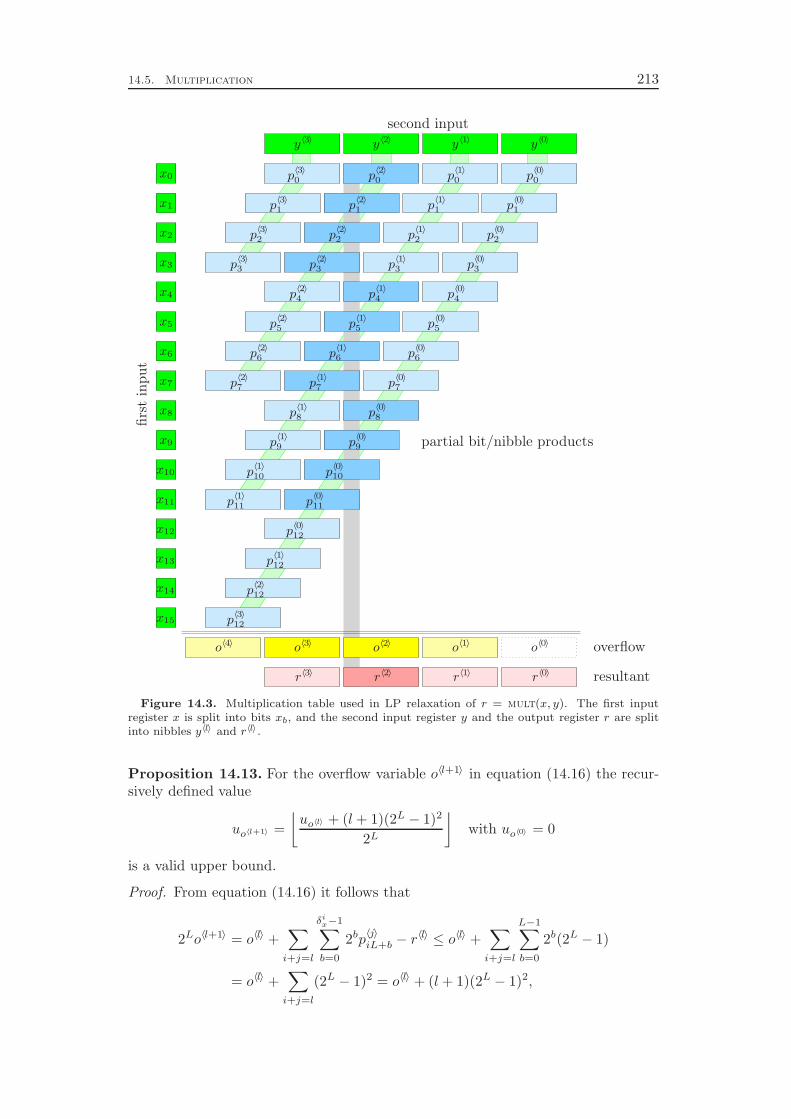
14.5. Multiplication 213
y〈0〉y〈1〉y〈2〉y〈3〉
x0
x1
x2
x3
x4
x5
x6
x7
x8
x9
x10
x11
x12
x13
x14
x15
o〈0〉o〈1〉o〈2〉o〈3〉o〈4〉
r〈0〉r〈1〉r〈2〉r〈3〉
p〈0〉0p
〈1〉0p
〈2〉0p
〈3〉0
p〈0〉1p
〈1〉1p
〈2〉1p
〈3〉1
p〈0〉2p
〈1〉2p
〈2〉2p
〈3〉2
p〈0〉3p
〈1〉3p
〈2〉3p
〈3〉3
p〈0〉4p
〈1〉4p
〈2〉4
p〈0〉5p
〈1〉5p
〈2〉5
p〈0〉6p
〈1〉6p
〈2〉6
p〈0〉7p
〈1〉7p
〈2〉7
p〈0〉8p
〈1〉8
p〈0〉9p
〈1〉9
p〈0〉10p
〈1〉10
p〈0〉11p
〈1〉11
p〈0〉12
p〈1〉12
p〈2〉12
p〈3〉12
firs
tin
put
second input
partial bit/nibble products
overflow
resultant
Figure 14.3. Multiplication table used in LP relaxation of r = mult(x, y). The first inputregister x is split into bits xb, and the second input register y and the output register r are splitinto nibbles y〈l〉 and r〈l〉.
Proposition 14.13. For the overflow variable o〈l+1〉 in equation (14.16) the recur-sively defined value
uo〈l+1〉 =
⌊uo〈l〉 + (l + 1)(2L − 1)2
2L
⌋
with uo〈0〉 = 0
is a valid upper bound.
Proof. From equation (14.16) it follows that
2Lo〈l+1〉 = o〈l〉 +∑
i+j=l
δix−1∑
b=0
2bp〈j〉iL+b − r
〈l〉 ≤ o〈l〉 +∑
i+j=l
L−1∑
b=0
2b(2L − 1)
= o〈l〉 +∑
i+j=l
(2L − 1)2 = o〈l〉 + (l + 1)(2L − 1)2,
214 Operators in Detail
which, together with the integrality of o〈l+1〉, proves the claim.
Note. The upper bounds on the first seven overflow variables are u〈0〉 = 0, u〈1〉 = 254,u〈2〉 = 509, u〈3〉 = 764, u〈4〉 = 1019, u〈5〉 = 1274, and u〈6〉 = 1529.
As a summary, the LP relaxation of a multiplication constraint r = mult(x, y)is given by equations (14.13), (14.14), and (14.15) for all b and l with ⌊b/L⌋+ l < ηr,and equation (14.16) for l = 0, . . . , ηr − 1. We have to introduce auxiliary variables
p〈l〉b ∈ R≥0 for ⌊b/L⌋ + l < ηr with bounds 0 ≤ p
〈l〉b ≤ uy〈l〉 , and o〈l〉 ∈ Z≥0 for
l = 0, . . . , ηr with bounds 0 ≤ o〈l〉 ≤ uo〈l〉 as defined in Proposition 14.13.
14.5.2 Domain Propagation
The propagation of multiplication constraints r = mult(x, y) is performed in threestages. The first stage applies domain propagation on the LP formulation stated
in Section 14.5.1 and its auxiliary variables p〈l〉b and o〈l〉. In the second stage, we
perform domain propagation on a multiplication table consisting of binary partialproducts pij = xi · yj , i.e., on a formulation that can be expressed with binaryvariables only. The third stage applies a symbolic propagation on this binarymultiplication table by using a term rewriting system.
Propagation on the LP Relaxation
In this stage of the propagation, we try to deduce tighter bounds for the bits xb, the
nibbles y〈l〉 and r〈l〉, and the auxiliary variables p〈l〉b and o〈l〉, which are used in the
LP relaxation presented in Section 14.5.1. Since it can yield tighter bounds for thepropagation, we also look at the current bounds of the partial bit product variablespij = xi · yj ∈ {0, 1} that are used in the next stage of the domain propagation.
As already noted in Section 14.5.1, the bounds of the nibbles y〈l〉 and r〈l〉 are onlyshortcuts for the sums of the corresponding bit bounds, see equation (14.12). Thesebounds get strengthened in presolving and domain propagation whenever one of theinvolved bits is fixed. Conversely, a strengthening of a nibble bound corresponds tofixings of the involved bits. However, for given deduced nibble bounds l ≤ y〈l〉 ≤ u,we can only fix the most significant bits ylL+b, namely ylL+b = 1 for bits b with∑δ−1
i=0 2iuylL+i−2buylL+b
< l, and ylL+b = 0 for bits b with∑δ−1
i=0 2ilylL+i−2blylL+b
+
2b > u. If we deduce l ≤ y〈l〉 ≤ u in an algorithm, we mean to fix as many bitvariables as possible in this fashion. The same holds for deduced nibble bounds onr〈l〉. Note that variables o〈l〉 are actual problem variables for which the bounds canbe deduced normally.
Algorithm 14.7 shows how the deductions on the registers x, y, and r, and theauxiliary variables of the LP relaxation are performed. Step 1 processes the partial
product equation p〈l〉b = xb · y
〈l〉. If xb = 0 we can conclude p〈l〉b = 0 in Step 1a. If on
the other hand xb = 1, we can tighten the bounds of p〈l〉b and y〈l〉 using p
〈l〉b = y〈l〉 in
Step 1b. Independent from the value of xb, the partial product p〈l〉b cannot be larger
than y〈l〉, and the upper bound of p〈l〉b and the lower bound of y〈l〉 can be tightened
correspondingly in Step 1c.
Step 1d provides the link to the auxiliary partial bit product variables pij = xi ·yj
which are used in the second stage of the domain propagation, see Algorithm 14.8.
14.5. Multiplication 215
Algorithm 14.7 Multiplication Domain Propagation – LP Propagation
Input : Multiplication constraint r = mult(x, y) on registers r, x, and y of widthβ with current local word bounds lrw ≤ rw ≤ urw , lxw ≤ xw ≤ uxw , andlyw ≤ yw ≤ uyw , and bit bounds lrb
≤ rb ≤ urb, lxb
≤ xb ≤ uxb, and lyb
≤
yb ≤ uyb; current local bounds on auxiliary variables l
p〈l〉b
≤ p〈l〉b ≤ u
p〈l〉b
,
lpij≤ pij ≤ upij
, and lo〈l〉 ≤ o〈l〉 ≤ uo〈l〉 .
Output : Tightened local bounds for words rw, xw, yw, bits rb, xb, yb, and auxiliary
variables p〈l〉b and o〈l〉.
1. For all b = 0, . . . , β − 1 and all l = 0, . . . , η − 1:
(a) If uxb= 0, deduce p
〈l〉b = 0.
(b) If lxb= 1, deduce p
〈l〉b ≥ ly〈l〉 and y〈l〉 ≤ u
p〈l〉b
.
(c) Deduce p〈l〉b ≤ uy〈l〉 and y〈l〉 ≥ l
p〈l〉b
.
(d) Deduce p〈l〉b ≤
∑L−1i=0 2iupb,lL+i
.
(e) If lp〈l〉b
≥ 1, deduce xb = 1.
(f) If up〈l〉b
< ly〈l〉 , deduce xb = 0.
2. For l = 0, . . . , η − 1, tighten the bounds using equation (14.16):
lr〈l〉 −∑
i+j=l
δix−1∑
b=0
2bup〈j〉iL+b
+ 2Llo〈l+1〉 ≤ o〈l〉 ≤ ur〈l〉 −∑
i+j=l
δix−1∑
b=0
2b lp〈j〉iL+b
+ 2Luo〈l+1〉
lo〈l〉 +∑
i+j=l
δix−1∑
b=0
2b lp〈j〉iL+b
− 2Luo〈l+1〉 ≤ r〈l〉 ≤ uo〈l〉 +∑
i+j=l
δix−1∑
b=0
2bup〈j〉iL+b
− 2Llo〈l+1〉
⌈ lo〈l〉 +∑
i+j=l
δix−1∑
b=0
2blp〈j〉iL+b
− ur〈l〉
2L
⌉
≤ o〈l+1〉 ≤
⌊ uo〈l〉 +∑
i+j=l
δix−1∑
b=0
2bup〈j〉iL+b
− lr〈l〉
2L
⌋
By the definition of the partial products, we know that p〈l〉b =
∑L−1i=0 2ipb,lL+i. There-
fore, we can deduce a corresponding upper bound for p〈l〉b in Step 1d. The lower bound
of p〈l〉b does not need to be tightened, because if
∑L−1i=0 2i lpb,lL+i
> 0 we can deduce
xb = 1 in Algorithm 14.8, and the lower bound of p〈l〉b is already tightened in a subse-
quent Step 1b of Algorithm 14.7. Note that after Algorithm 14.8 was performed, wehave
∑L−1i=0 2iupb,lL+i
≤ uy〈l〉 , which means that Step 1c is redundant in subsequentiterations.
Steps 1e and 1f are the inverse implications of Steps 1a and 1b, respectively. If
p〈l〉b > 0, the bit xb must be one, and if p
〈l〉b < y〈l〉, we know that xb = 0. Additional
conclusions like p〈l〉b = 0 if p
〈l〉b < y〈l〉 are automatically drawn in Steps 1a and 1b of
the subsequent iteration.
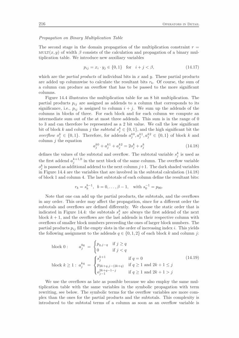
216 Operators in Detail
Propagation on Binary Multiplication Table
The second stage in the domain propagation of the multiplication constraint r =mult(x, y) of width β consists of the calculation and propagation of a binary mul-tiplication table. We introduce new auxiliary variables
pij = xi · yj ∈ {0, 1} for i+ j < β, (14.17)
which are the partial products of individual bits in x and y. These partial productsare added up columnwise to calculate the resultant bits rb. Of course, the sum ofa column can produce an overflow that has to be passed to the more significantcolumns.
Figure 14.4 illustrates the multiplication table for an 8 bit multiplication. Thepartial products pij are assigned as addends to a column that corresponds to itssignificance, i.e., pij is assigned to column i + j. We sum up the addends of thecolumns in blocks of three. For each block and for each column we compute anintermediate sum out of the at most three addends. This sum is in the range of 0to 3 and can therefore be represented as a 2 bit value. We call the low significantbit of block k and column j the subtotal sk
j ∈ {0, 1}, and the high significant bit the
overflow okj ∈ {0, 1}. Therefore, for addends ak0
j , ak1j , ak2
j ∈ {0, 1} of block k andcolumn j the equation
ak0j + ak1
j + ak2j = 2ok
j + skj (14.18)
defines the values of the subtotal and overflow. The subtotal variable skj is used as
the first addend ak+1,0j in the next block of the same column. The overflow variable
okj is passed as additional addend to the next column j+1. The dark shaded variables
in Figure 14.4 are the variables that are involved in the subtotal calculation (14.18)of block 1 and column 4. The last subtotals of each column define the resultant bits:
rb = sb−1b , b = 0, . . . , β − 1, with s−1
0 = p00.
Note that one can add up the partial products, the subtotals, and the overflowsin any order. This order may affect the propagation, since for a different order thesubtotals and overflows are defined differently. We choose the static order that isindicated in Figure 14.4: the subtotals sk
j are always the first addend of the nextblock k + 1, and the overflows are the last addends in their respective column withoverflows of smaller block numbers preceeding the ones of larger block numbers. Thepartial products pij fill the empty slots in the order of increasing index i. This yieldsthe following assignment to the addends q ∈ {0, 1, 2} of each block k and column j:
block 0 : a0qj =
{
pq,j−q if j ≥ q
0 if j < q
block k ≥ 1 : akqj =
sk+1j if q = 0
p2k+q,j−(2k+q) if q ≥ 1 and 2k + 1 ≤ j
o2k+q−1−jj−1 if q ≥ 1 and 2k + 1 > j
(14.19)
We use the overflows as late as possible because we also employ the same mul-tiplication table with the same variables in the symbolic propagation with termrewriting, see below. The symbolic terms for the overflow variables are more com-plex than the ones for the partial products and the subtotals. This complexity isintroduced to the subtotal terms of a column as soon as an overflow variable is
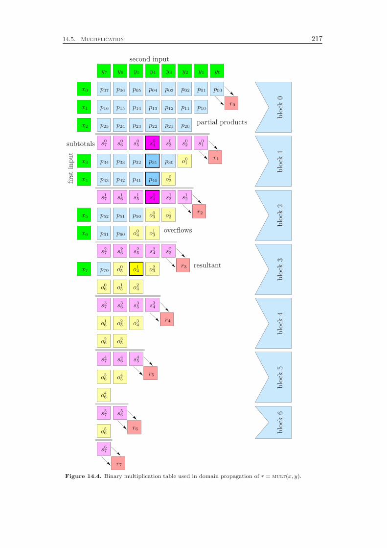
14.5. Multiplication 217
x0
x1
x2
x3
x4
x5
x6
x7
y0y1y2y3y4y5y6y7
r0
r1
r2
r3
r4
r5
r6
r7
p00p01p02p03p04p05p06p07
p10p11p12p13p14p15p16
p20p21p22p23p24p25
p30p31p32p33p34
p40p41p42p43
p50p51p52
p60p61
p70
s01s02s03s04s05s06s07
s12s13s14s15s16s17
s23s24s25s26s27
s34s35s36s37
s45s46s47
s56s57
s67
o01
o02
o03
o04
o05
o06
o12
o13
o14
o15
o16
o23
o24
o25
o26
o34
o35
o36 o45
o46
o56
blo
ck0
blo
ck1
blo
ck2
blo
ck3
blo
ck4
blo
ck5
blo
ck6
firs
tin
put
second input
partial products
subtotals
overflows
resultant
Figure 14.4. Binary multiplication table used in domain propagation of r = mult(x, y).
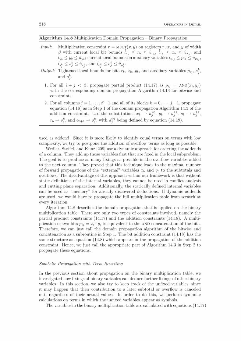
218 Operators in Detail
Algorithm 14.8 Multiplication Domain Propagation – Binary Propagation
Input : Multiplication constraint r = mult(x, y) on registers r, x, and y of widthβ with current local bit bounds lrb
≤ rb ≤ urb, lxb
≤ xb ≤ uxb, and
lyb≤ yb ≤ uyb
; current local bounds on auxiliary variables lpij≤ pij ≤ upij
,
lskj≤ sk
j ≤ uskj, and lok
j≤ ok
j ≤ uokj.
Output : Tightened local bounds for bits rb, xb, yb, and auxiliary variables pij , skj ,
and okj .
1. For all i + j < β, propagate partial product (14.17) as pij = and(xi, yj)with the corresponding domain propagation Algorithm 14.13 for bitwise andconstraints.
2. For all columns j = 1, . . . , β−1 and all of its blocks k = 0, . . . , j−1, propagateequation (14.18) as in Step 1 of the domain propagation Algorithm 14.3 of theaddition constraint. Use the substitutions xb → ak0
j , yb → ak1j , ob → ak2
j ,
rb → skj , and ob+1 → ok
j , with akqj being defined by equation (14.19).
used as addend. Since it is more likely to identify equal terms on terms with lowcomplexity, we try to postpone the addition of overflow terms as long as possible.
Wedler, Stoffel, and Kunz [209] use a dynamic approach for ordering the addendsof a column. They add up those variables first that are fixed in the local subproblem.The goal is to produce as many fixings as possible in the overflow variables addedto the next column. They proved that this technique leads to the maximal numberof forward propagations of the “external” variables xb and yb to the subtotals andoverflows. The disadvantage of this approach within our framework is that withoutstatic definitions of the internal variables, they cannot be used in conflict analysisand cutting plane separation. Additionally, the statically defined internal variablescan be used as “memory” for already discovered deductions. If dynamic addendsare used, we would have to propagate the full multiplication table from scratch atevery iteration.
Algorithm 14.8 describes the domain propagation that is applied on the binarymultiplication table. There are only two types of constraints involved, namely thepartial product constraints (14.17) and the addition constraints (14.18). A multi-plication of two bits pij = xi · yj is equivalent to the and concatenation of the bits.Therefore, we can just call the domain propagation algorithm of the bitwise andconcatenation as a subroutine in Step 1. The bit addition constraint (14.18) has thesame structure as equation (14.8) which appears in the propagation of the additionconstraint. Hence, we just call the appropriate part of Algorithm 14.3 in Step 2 topropagate these equations.
Symbolic Propagation with Term Rewriting
In the previous section about propagation on the binary multiplication table, weinvestigated how fixings of binary variables can deduce further fixings of other binaryvariables. In this section, we also try to keep track of the unfixed variables, sinceit may happen that their contribution to a later subtotal or overflow is canceledout, regardless of their actual values. In order to do this, we perform symboliccalculations on terms in which the unfixed variables appear as symbols.
The variables in the binary multiplication table are calculated with equations (14.17)

14.5. Multiplication 219
and (14.18), i.e.,
pij = xi · yj and 2okj + sk
j = ak0j + ak1
j + ak2j ,
with akqj being either a partial product p, a subtotal s, or an overflow o. Now we
express the equations to calculate p, s, and o as logical terms over xi and yj :
pij = xi ∧ yj (14.20)
skj = ak0
j ⊕ ak1j ⊕ a
k2j (14.21)
okj = (ak0
j ∧ ak1j ) ∨ (ak0
j ∧ ak2j ) ∨ (ak1
j ∧ ak2j )
= (ak0j ∧ a
k1j )⊕(ak0
j ∧ ak2j )⊕(ak1
j ∧ ak2j ). (14.22)
We can replace the disjunction ∨ by the exclusive or ⊕ in the equation of okj , because
it cannot happen that exactly two of the three subterms are true, and in the otherthree cases (0, 1, or 3 terms are true), both operators yield the same result:
Observation 14.14. For all x, y, z ∈ {0, 1}, the equivalence
(x ∨ y ∨ z 6= x⊕ y⊕ z) ⇔ (x+ y + z = 2)
holds.
Proof. We only have to evaluate the four cases x + y + z ∈ {0, 1, 2, 3}, since bothoperators ∨ and ⊕ are associative and commutative.
Due to Observation 14.14, we can express all emerging expressions for internalvariables in the binary multiplication table as terms over ∧ and ⊕. We call theresulting algebra the binary multiplication term algebra:
Definition 14.15 (binary multiplication signature). The algebraic signatureΣ = (B,O) with the sort B and operations O = O0 ∪ O2 with 0-ary symbolsO0 = {0, 1, x0, . . . , xβ−1, y0, . . . , yβ−1} and binary operators O2 = {∧,⊕},
0 :→ B, 1 :→ B, xb :→ B, yb :→ B, ∧ : B ×B → B, ⊕ : B × B → B
with b = 0, . . . , β − 1 is called binary multiplication signature. We call TΣ the termalgebra of Σ, which consists of all terms that can be generated from the symbols inΣ and which fit to the arity of the operators.
By applying the distributivity law
(s⊕ t) ∧ u = (s ∧ u)⊕(t ∧ u), s ∧ (t⊕u) = (s ∧ t)⊕(s ∧ u)
for terms s, t, u ∈ TΣ we can rewrite any term t ∈ TΣ as an equivalent term indisjunctive normal form
t ≡ πn⊕ . . .⊕π1, πi = zimi∧ . . . ∧ zi1, zij ∈ O0
for i = 1, . . . , n and j = 1, . . . ,mi. Due to commutativity and associativity of ∧, theindividual conjunctions can be reordered in a second step such that
πi = zimi∧ . . . ∧ zi1 with zimi
� . . . � zi1

220 Operators in Detail
holds for the precedence relation ≻ on the symbols O of Σ, which is defined as thetransitive closure of
∧ ≻ ⊕ ≻ yβ−1 ≻ . . . ≻ y0 ≻ xβ−1 ≻ . . . ≻ x0 ≻ 1 ≻ 0. (14.23)
Afterwards, we apply the equations
z ∧ 0 = 0, z ∧ 1 = z, z ∧ z = z
on the conjunctions which yields equivalent conjunctions in normal form. The ad-dends πi of a term t ∈ TΣ in disjunctive normal form with normalized conjunctionsare then reordered using commutativity and associativity of ⊕ such that
t ≡ πn⊕ . . .⊕π1, πi = zimi∧ . . . ∧ zi1, zij ∈ O0
and (zimi, . . . , zi1) �lex (zjmj
, . . . , zj1) for i > j. The relation ≻lex is the lexico-graphic (right-left) ordering with respect to ≻:
Definition 14.16 (lexicographic ordering). Given an ordering ≻⊆ O × O on aset O, the relation ≻lex⊆ O
⋆ × O⋆ on the strings O⋆ with
(tn, . . . , t1) ≻lex (sm, . . . , s1)
⇔ (i) n > m, or
(ii) n = m and t1 ≻ s1, or
(iii) n = m and t1 = s1 and (tn, . . . , t2) ≻lex (sm, . . . , s2)
is called lexicographic (right-left) ordering with respect to ≻ on strings O⋆.
Note. The literature distinguishes between two versions of the lexicographic order-ing: the left-right ordering ≻lexlr and the right-left ordering ≻lexrl. Since we onlyneed the right-left variant, we abbreviate ≻lexrl by ≻lex and call this version thelexicographic ordering as a shortcut.
After having reordered the addends of the disjunction, we simplify the term byapplying the equations
π⊕ 0 = π and π⊕π = 0.
We call the resulting term t′ the normal form of t if t ≡ t′.Algorithm 14.9 subsumes this procedure in a more formal fashion. In Step 1
we apply the distributivity law to achieve disjunctive normal form. Step 2 reordersthe symbols in the conjunctions πi, and Step 3 applies the simplifications for the ∧operator. Note that these simplifications do not destroy the ordering property ofthe conjunctions. In Step 4 we reorder the resulting addends of the xor expression,and finally, in Step 5 the simplifications on the ⊕ operator are applied. The replace-ment 5b replaces the innermost two addends of the term by the symbol “0”, whichhas to be moved to the right by applying Step 4 again to restore the lexicographicordering.
In the definition of the commutativity rewriting Rules 4b and 4c we used theconcept of the lexicographic recursive path ordering (see Kamin and Levy [128] andDershowitz [79]):

14.5. Multiplication 221
Algorithm 14.9 Multiplication Domain Propagation – Term Normalization
Input : Term t ∈ TΣOutput : Term t′ ≡ t in normal form
1. Until no more replacements are possible:
(a) Replace subterms (t3⊕ t2) ∧ t1 → (t3 ∧ t1)⊕(t2 ∧ t1).
(b) Replace subterms t3 ∧ (t2⊕ t1)→ (t3 ∧ t2)⊕(t3 ∧ t1).
2. Until no more replacements are possible:
(a) Replace subterms π3 ∧ (π2 ∧ π1)→ (π3 ∧ π2) ∧ π1.
(b) Replace subterms z1 ∧ z2 → z2 ∧ z1 if z1, z2 ∈ O0 and z2 ≻ z1.
(c) Replace subterms (π ∧ z1)∧ z2 → (π ∧ z2)∧ z1 if z1, z2 ∈ O0 and z2 ≻ z1.
3. Until no more replacements are possible:
(a) Replace subterms π ∧ 0→ 0.
(b) Replace subterms π ∧ 1→ π.
(c) Replace subterms z ∧ z → z with z ∈ O0.
(d) Replace subterms (π ∧ z) ∧ z → π ∧ z with z ∈ O0.
4. Until no more replacements are possible:
(a) Replace subterms π3⊕(π2⊕π1)→ (π3⊕π2)⊕π1.
(b) Replace subterms π1⊕π2 → π2⊕ π1 if π2 ≻lrpo π1.
(c) Replace subterms (π3⊕ π1)⊕π2 → (π3⊕ π2)⊕π1 if π2 ≻lrpo π1.
5. Until no more replacements are possible:
(a) Replace subterms π⊕ 0→ π.
(b) Replace subterms π⊕π → 0; if applied, goto Step 4.
(c) Replace subterms (π2⊕ π1)⊕π1 → π2.
Definition 14.17 (lexicographic recursive path ordering). Let Σ = (S,O) bean algebraic signature and ≻⊆ O×O be a partial ordering on the operator symbolsof Σ. Then ≻lrpo⊆ TΣ × TΣ with
g(tn, . . . , t1) ≻lrpo f(sm, . . . , s1)
⇔ (i) tj �lrpo f(sm, . . . , s1) for some j ∈ {1, . . . , n}, or
(ii) g ≻ f and g(tn, . . . , t1) ≻lrpo si for all i ∈ {1, . . . ,m}, or
(iii) g = f, g(tn, . . . , t1) ≻lrpo si for all i ∈ {1, . . . ,m},
and (tn, . . . , t1) (≻lrpo)lex (sm, . . . , s1)
is called the lexicographic recursive path ordering of Σ with respect to ≻.
Note again, that we employ the right-left variant of the lexicographic ordering inour definition of ≻lrpo.
The lexicographic recursive path ordering is a very useful tool for proving thetermination of term rewriting systems. In the following, we employ this concept toprove the termination of Algorithm 14.9.
222 Operators in Detail
Lemma 14.18. Let Σ = (S,O) be an algebraic signature and ≻⊆ O × O a partialordering on the operator symbols. If s ∈ TΣ is a proper subterm of t ∈ TΣ thent ≻lrpo s.
Proof. We prove the claim by induction on the depth d ∈ Z>0 of s in the treerepresentation of t = g(tn, . . . , t1). If s = tj for any j ∈ {1, . . . , n}, i.e., d = 1, wehave t ≻lrpo s by Condition (i) of Definition 14.17. Otherwise, let tj be the subtermof t that contains s. Then, s is in depth d − 1 of the tree representation of tj , andwe have tj ≻lrpo s by induction. Again by Condition (i), it follows t ≻lrpo s.
Definition 14.19 (well-founded ordering). A partial ordering ≻⊆ S × S ona set S is called well-founded if there does not exist an infinite descending chains1 ≻ s2 ≻ . . . of elements si ∈ S.
Definition 14.20 (monotonic ordering). Given an algebraic signature Σ = (S,O)with term algebra TΣ, a partial ordering ≻⊆ TΣ × TΣ on the terms is called mono-tonic, if
s ≻ s′ ⇒ g(tn, . . . , s, . . . , t1) ≻ g(tn, . . . , s′, . . . , t1)
for all n ∈ Z≥0, n-ary symbols g ∈ O, and terms s, s′, t1, . . . , tn ∈ TΣ.
Theorem 14.21 (Dershowitz [79]). If≻⊆ O×O is a well-founded partial orderingon the operations of a finite algebraic signature Σ = (S,O), then the lexicographicrecursive path ordering ≻lrpo⊆ TΣ×TΣ is a well-founded monotonic partial orderingon the terms TΣ.
For our precedence relation≻ defined by (14.23), the lexicographic recursive pathordering ≻lrpo⊆ TΣ × TΣ of Σ with respect to ≻ is given by
z2 ≻lrpo z1 if z2 ≻ z1 (a)
t2⊕ t1 ≻lrpo z (b)
t2 ∧ t1 ≻lrpo z (c)
t2⊕ t1 ≻lrpo s2⊕ s1 if t1 �lrpo s2⊕ s1 or t2 �lrpo s2⊕ s1 (d)
t2⊕ t1 ≻lrpo s2 ∧ s1 if t1 �lrpo s2 ∧ s1 or t2 �lrpo s2 ∧ s1 (e)
t2 ∧ t1 ≻lrpo s2⊕ s1 if t1 �lrpo s2⊕ s1 or t2 �lrpo s2⊕ s1 (f)
t2 ∧ t1 ≻lrpo s2 ∧ s1 if t1 �lrpo s2 ∧ s1 or t2 �lrpo s2 ∧ s1 (g)
t2 ∧ t1 ≻lrpo s2⊕ s1 if t2 ∧ t1 ≻lrpo si for i = 1, 2 (h)
t2⊕ t1 ≻lrpo s2⊕ s1 if t2⊕ t1 ≻lrpo si for i = 1, 2, and t1 ≻lrpo s1 (i)
t2⊕ t1 ≻lrpo s2⊕ s1 if t2⊕ t1 ≻lrpo si for i = 1, 2, and t1 = s1, t2 ≻lrpo s2 (j)
t2 ∧ t1 ≻lrpo s2 ∧ s1 if t2 ∧ t1 ≻lrpo si for i = 1, 2, and t1 ≻lrpo s1 (k)
t2 ∧ t1 ≻lrpo s2 ∧ s1 if t2 ∧ t1 ≻lrpo si for i = 1, 2, and t1 = s1, t2 ≻lrpo s2 (l)
for all z, z1, z2 ∈ O0, s1, s2, t1, t2 ∈ TΣ.
Proposition 14.22. Algorithm 14.9 terminates.
Proof. The relation ≻ is obviously a well-founded partial ordering (in fact, even atotal ordering) on O. By Theorem 14.21 ≻lrpo is a well-founded monotonic partial
14.5. Multiplication 223
ordering on TΣ. Therefore, to show the termination of Algorithm 14.9 it sufficesto prove that each replacement rule reduces the order of the term t, i.e., if t isreplaced by t′, then t ≻lrpo t
′. Due to the monotonicity, it even suffices to show thisimplication for the subterms on which the replacements are applied.
Step 1a reduces the order due to condition (h) since (t3⊕ t2) ∧ t1 ≻lrpo t3 ∧ t1and (t3⊕ t2) ∧ t1 ≻lrpo t2 ∧ t1 by condition (l) and Lemma 14.18. The same is truefor Step 1b by condition (h), condition (k), and Lemma 14.18. Step 2a reduces theorder due to (k) and Lemma 14.18. Step 2b is due to (k), (a), and Lemma 14.18,and the order reduction of Step 2c follows from (k), (a), (l), and Lemma 14.18.
The replacements in Step 3 reduce the order of the term due to Lemma 14.18.The proof for the replacements in Step 4 is analogous to the one for Step 2. Theorder reduction of Step 5a and 5c is again due to Lemma 14.18 and follows forStep 5b by condition (b).
Corollary 14.23. Algorithm 14.9 would also terminate if the term rewriting ruleswere applied in an arbitrary order.
Proof. Since each individual rewriting rule reduces the order of the term, terminationis not dependent on the order in which they are applied.
After having defined our term rewriting system in Algorithm 14.9 to normalizearbitrary terms t ∈ TΣ, we are ready to present the term algebra domain propagationalgorithm for mult constraints, which is illustrated in Algorithm 14.10. Thealgorithm consists of a loop over the columns and addition blocks of the binarymultiplication table of Figure 14.4, i.e., over the individual equations (14.18). Theterms are calculated and processed in Steps 2 to 6. If deductions or substitutions inthe terms have been found, the loop counters are reset in Step 8 to reevaluate theaffected additions.
In Step 2 we identify the addends that are used in the sum calculated in thecurrent part of the addition table. If an addend is a partial product, we constructthe corresponding term, normalize it, and propagate the variable-term equation inStep 3. If an addend is a subtotal or an overflow, we already constructed andprocessed the term in a previous iteration of the loop. Steps 4, 5, and 6 performthis term construction, normalization, and processing for the current subtotal andoverflow.
If in the local subproblem only a few variables are fixed such that only a fewpropagations and substitutions can be performed, the terms for the subtotals andoverflows can grow very quickly. This results in a large consumption of memory andprocessing time. In order to avoid such a large resource consumption, we abort thealgorithm if the number of addends in a normalized subtotal term exceeds a certainvalue. In our implementation, we use the limit maxaddends = 20.
The propagation of a variable-term equation ξ = t(z1, . . . , zm), t ∈ TΣ, which isperformed in Steps 3c and 6 of Algorithm 14.10 is depicted in Algorithm 14.11. Ifthe term is equal to t = 0 or t = 1, the variable ξ can be fixed to the correspondingvalue in Step 1. If the term consists of only one variable symbol z1 and the variableξ is fixed, we can also fix z1 to the same value in Step 2a. If ξ = 1, we can evenfix all term variables to zi = 1 in Step 2b if the term has only one addend. If theterm only consists of one addend π1 but no fixings could be deduced, we can at leastreplace all occurrences of π1 in the other terms produced by Algorithm 14.10 withξ. This substitution is performed in Step 2c. Since 1⊕π = ¬π, we can also apply

224 Operators in Detail
Algorithm 14.10 Multiplication Domain Propagation – Symbolic Propagation
Input : Multiplication constraint r = mult(x, y) on registers r, x, and y of widthβ with current local bit bounds lrb
≤ rb ≤ urb, lxb
≤ xb ≤ uxb, and
lyb≤ yb ≤ uyb
; current local bounds on auxiliary variables lpij≤ pij ≤ upij
,
lskj≤ sk
j ≤ uskj, and lok
j≤ ok
j ≤ uokj; Parameter maxaddends ∈ N.
Output : Tightened local bounds for bits rb, xb, yb, and auxiliary variables pij , skj ,
and okj .
1. Set j := 0 and k := 0.
2. Identify the addends ak0j , ak1
j , ak2j of column j, block k by equation (14.19).
3. For all q with akqj = pbb′ for bits b and b′:
(a) Assign the term t[pbb′ ] := xb ∧ yb′ as in (14.20).
(b) Normalize t[pbb′ ] by calling Algorithm 14.9.
(c) Propagate pbb′ = t[pbb′ ] with Algorithm 14.11.
4. Assign the terms
t[skj ] := t[ak0
j ]⊕ t[ak1j ]⊕ t[ak2
j ]
and t[okj ] := (t[ak0
j ] ∧ t[ak1j ])⊕(t[ak0
j ] ∧ t[ak2j ])⊕(t[ak1
j ] ∧ t[ak2j ])
as in (14.21) and (14.22).
5. Normalize t[skj ] and o[sk
j ] by calling Algorithm 14.9.
6. Propagate skj = t[sk
j ] and okj = t[ok
j ] with Algorithm 14.11.
7. If t[skj ] = π1⊕ . . .⊕ πn and n > maxaddends, stop.
8. If at least one of the calls of Algorithm 14.11 produced a fixing of a variableor a substitution in a term, set j to be the minimal column and set k to bethe minimal block number in this column for which a participating term wasaffected.
Otherwise, set k := k + 1. If k ≥ j, set j := j + 1 and k := 0.
9. If j < β, goto Step 2.
the reasoning of Step 2 to t = 1⊕ π2, which is done in Step 3. However, we have toconsider ξ in its negated version since
ξ = 1⊕π2(z1, . . . , zm) ⇔ ¬ ξ = π2(z1, . . . , zm).
If t = π1⊕ π2 consists of exactly two addends and ξ is fixed, we can draw thefollowing conclusions in Step 4. If ξ = 0, it follows π1 = π2 which allows propagationin Step 4a or substitution in Step 4c, depending on whether π1 is a single variablesymbol or not. If ξ = 1, analogous reasoning can be applied in Steps 4b and 4d.Again, a term t = 1⊕π2⊕π3 can be processed in the same fashion by negating thevalue of ξ, which is performed in the final Step 5.

14.5. Multiplication 225
Algorithm 14.11 Multiplication Domain Propagation – Variable-Term Equation
Input : Equation ξ = t(z1, . . . , zm) with ξ being a binary CIP variable and t ∈ TΣbeing a normalized term t = π1⊕ . . .⊕ πn with 0-ary symbols z1, . . . , zm ∈O0; current local bit bounds lξ ≤ ξ ≤ uξ and lzj
≤ zj ≤ uzjfor the CIP
variables corresponding to the involved 0-ary symbols.
Output : Tightened local bounds for bits ξ, z1, . . . , zm; Modifications of the termss ∈ T produced by Algorithm 14.10.
1. If t = 0, deduce ξ = 0.If t = 1, deduce ξ = 1.
2. If t = π1:
(a) If π1 = z1 and uξ = 0, deduce z1 = 0.
(b) If π1 = z1 ∧ . . . ∧ zm and lξ = 1, deduce zj = 1 for all j = 1, . . . ,m.
(c) If neither 2a nor 2b was applied and ξ ∈ O0, substitute t→ ξ in all termss ∈ T .
3. If t = 1⊕π2:
(a) If π2 = z1 and lξ = 1, deduce z1 = 0.
(b) If π2 = z1 ∧ . . . ∧ zm and uξ = 0, deduce zj = 1 for all j = 1, . . . ,m.
(c) If neither 3a nor 3b was applied and ξ ∈ O0, substitute t→ ξ in all termss ∈ T .
4. If t = π1⊕π2:
(a) If π1 = zj and uξ = 0, propagate zj = π2 as in Step 2.
(b) If π1 = zj and lξ = 1, propagate zj = 1⊕π2 as in Step 3.
(c) If π1 /∈ O0 and uξ = 0, substitute π2 → π1 in all terms s ∈ T .
(d) If π1 /∈ O0 and lξ = 1, substitute π2 → 1⊕π1 in all terms s ∈ T .
5. If t = 1⊕π2⊕π3:
(a) If π2 = zj and lξ = 1, propagate zj = π3 as in Step 2.
(b) If π2 = zj and uξ = 0, propagate zj = 1⊕π3 as in Step 3.
(c) If π2 /∈ O0 and lξ = 1, substitute π3 → π2 in all terms s ∈ T .
(d) If π2 /∈ O0 and uξ = 0, substitute π3 → 1⊕π2 in all terms s ∈ T .
14.5.3 Presolving
The presolving of multiplication constraints is performed as illustrated in Algo-rithm 14.12. Similar to the presolving of addition constraints, we first check forvery easy situations. If one of the operands is fixed to zero, the resultant can alsobe fixed to zero in Step 1a, and the multiplication constraint can be deleted. If anoperand is fixed to one, the resultant must always be equal to the other operand.They are aggregated in Step 1b, which also leads to the deletion of the constraint.If the resultant is zero, we could conclude that one of the operands must be zero ifthe constraint would be an ordinary multiplication r = x · y. However, this is notnecessarily true in the truncated multiplication. We can only fix an operand to zeroin Step 1c if the least significant bit of the other operand is one:

226 Operators in Detail
Algorithm 14.12 Multiplication Presolving
1. For all active multiplication constraints r = mult(x, y):
(a) If x = 0, fix r := 0 and delete the constraint.If y = 0, fix r := 0 and delete the constraint.
(b) If x = 1, aggregate r : ⋆= y and delete the constraint.If y = 1, aggregate r : ⋆= x and delete the constraint.
(c) If r = 0 and x0 = 1, fix y := 0 and delete the constraint.If r = 0 and y0 = 1, fix x := 0 and delete the constraint.
(d) If r ⋆= x and x0 = 1, fix y := 1 and delete the constraint.If r ⋆= y and y0 = 1, fix x := 1 and delete the constraint.
(e) If β = 1, replace the constraint by r = and(x, y).
(f) If maximal non-zero bit of y is less significant than the one of x, i.e.,max{b | uyb
= 1} < max{b | uxb= 1}, replace the constraint by r =
mult(y, x).
(g) Apply LP domain propagation Algorithm 14.7 on the global bounds.
(h) Apply binary domain propagation Algorithm 14.8 on the global bounds,but additionally:
i. For all partial products pij = xi · yj , i + j < β, apply presolvingAlgorithm 14.14 for and constraints.
ii. For all columns j and blocks k in the binary multiplication table ofFigure 14.4, apply bit aggregation Algorithm 14.5 of add constraints.
(i) Apply symbolic domain propagation Algorithm 14.10 on the globalbounds. Whenever a substitution t→ u in Algorithm 14.11 is applied:
i. If t = ξ1 and u = ξ2, or t = 1⊕ ξ1 and u = 1⊕ ξ2 with CIP variablesξ1, ξ2, aggregate ξ1 : ⋆= ξ2.
ii. If t = ξ1 and u = 1⊕ ξ2, or t = 1⊕ ξ1 and u = ξ2 with CIP variablesξ1, ξ2, aggregate ξ1 : ⋆= 1− ξ2.
2. For all pairs of active multiplication constraints r = mult(x, y) and r′ =mult(x′, y′) with βr ≥ βr′ :
(a) For all b = 0, . . . , βr′ − 1:i. If x[b, 0] ⋆= x′[b, 0] and y[b, 0] ⋆= y′[b, 0], aggregate r[b, 0] : ⋆= r′[b, 0].
ii. If x[b, 0] ⋆= y′[b, 0] and y[b, 0] ⋆= x′[b, 0], aggregate r[b, 0] : ⋆= r′[b, 0].
(b) If Step 2(a)i or 2(a)ii was successfully applied for b = βr′ − 1, delete theconstraint r′ = mult(x′, y′).
(c) If βr = βr′ , x ⋆= x′, but r Y⋆= r′, deduce y Y
⋆= y′.
If βr = βr′ , y ⋆= y′, but r Y⋆= r′, deduce x Y
⋆= x′.
(d) If βr = βr′ , x ⋆= y′, but r Y⋆= r′, deduce y Y
⋆= x′.
If βr = βr′ , y ⋆= x′, but r Y⋆= r′, deduce x Y
⋆= y′.
14.5. Multiplication 227
Proposition 14.24. Let β ∈ Z>0 and p, q ∈ Z≥0 be two integers with p being odd,q < 2β, and 0 = (p · q) mod 2β. Then, it follows q = 0.
Proof. By definition of the modulus operator we have
0 = (p · q) mod 2β ⇔ ∃k ∈ Z : 2βk = p · q.
Since p is odd and 2βk is even for any k ∈ Z, q must be even. For β = 1 this meansq = 0. For larger β we divide both sides of the equation by 2, which yields
∃k ∈ Z : 2β−1k = p ·q
2⇔ 0 = (p ·
q
2) mod 2β−1.
Since q2 ∈ Z≥0 and q
2 < 2β−1, it follows q2 = 0 by induction and therefore q = 0.
If r = 0 and b ≥ 1 is the least significant bit for which xb = 1, we can onlyconclude that y[β−1− b, 0] = 1, since the more significant bits in y do not affect theresultant if xb′ = 0 for all b′ < b. Such deductions are already detected in Step 1h.Therefore, we only consider the cases x0 = 1 and y0 = 1 in Step 1c which in additionto the fixings allow the deletion of the multiplication constraint.
The equivalences r ⋆= x and r ⋆= y are treated in Step 1d. For r ⋆= x we canconclude
x = mult(x, y) ⇔ x = (x · y) mod 2β ⇔ 0 =(x · (y − 1)
)mod 2β,
and by Proposition 14.24 it follows y = 1 if the least significant bit of x is x0 = 1.Again, the deductions for xb = 1 with b ≥ 1 are performed in Step 1h.
The special situation of a single-bit multiplication is addressed in Step 1e. Forβ = 1 we have mult(x, y) = and(x, y). Since the and constraint comes with an LPrelaxation without auxiliary variables (see Section 14.7.1) and features a much lesscumbersome propagation algorithm, we replace single-bit mult constraints by andconstraints.
In the LP relaxation of the multiplication constraint r = mult(x, y), the secondoperand y is split into nibbles while the first operand x is used in its bit represen-tation. Thus, the interchange of the operands leads to a different LP relaxation.
Different behavior can also appear in the domain propagation algorithms, sincefor r = mult(y, x) the multiplication tables of Figures 14.3 and 14.4 would changeas well as the definition of the auxiliary variables. We experimented with differentheuristic strategies for switching operands. The results indicated that the best strat-egy is to select the first operand x to be the one that has more high-significant bitsfixed to zero. Therefore, the constraint r = mult(x, y) is replaced by r = mult(y, x)in Step 1f if the position of the highest bit not fixed to zero is smaller in y than inx.
Step 1g applies domain propagation on the multiplication table of the LP re-laxation. We do not perform additional aggregations on the auxiliary variables ofthe LP relaxation for the following reason. The nibbles are not represented as CIPvariables. Instead, they are only shortcuts for a subword of the register’s bit string.Therefore, most of the possible aggregations would be multi-aggregations which areaggregations with more than one variable on the right hand side. In the currentversion of SCIP it is not possible to apply local bound changes to multi-aggregatedvariables, since this can only be realized by changing the left and right hand sidesof the corresponding inequality, which is not supported by the data structures of
SCIP. Take the aggregation p〈l〉b
⋆= y〈l〉 as an example, which could be applied if
228 Operators in Detail
xb = 1. In fact, this means to multi-aggregate p〈l〉b
⋆=∑δ−1
i=0 2iylL+i, which producesthe additional constraint
lp〈l〉b
≤δ−1∑
i=0
2iylL+i ≤ up〈l〉b
(14.24)
to reflect the bounds of p〈l〉b . Changing the local bounds of p
〈l〉b means to modify the
left and right hand side of inequality (14.24).In Step 1h of Algorithm 14.12 we perform the domain propagation on the binary
multiplication table. Additionally, aggregations are possible for the partial prod-uct equations (14.17) and the subtotal equations (14.18). In the symbolic domainpropagation of Step 1i, we can also perform aggregations whenever a substitutionwas found that identifies two terms containing only a single register bit or auxiliarybinary variable each.
Pairs of mult constraints are compared in Step 2. We can aggregate the sub-words of the resultants r[b, 0] : ⋆= r′[b, 0] in Step 2a if the corresponding subwordsof the operands in the two constraints are pairwise equivalent in any order. If thisaggregation was successfully performed on the full width of r′, we can delete thesecond constraint in Step 2b. Steps 2c and 2d deduce the inequality of the operandsby applying the implications of 2(a)i and 2(a)ii in the opposite direction. This isonly possible if the resultants are of equal width. Otherwise, the inequality of theresultants may result from the different truncation of the product.
14.6 Bitwise Negation
The bitwise negation operation
not : [β]→ [β], x 7→ r = not(x)
negates each individual bit such that
r = not(x) ⇔ ∀b ∈ {0, . . . , β − 1} : rb = 1− xb.
In order to implement such a constraint, we just have to aggregate the variablesrb : ⋆= 1 − xb, b = 0, . . . , β − 1, in the presolving stage of SCIP. Afterwards, theconstraint can be deleted from the problem formulation.
14.7 Bitwise And
The bitwise and combination of two bit vectors x, y ∈ {0, . . . , 2β−1} with x =∑β−1
b=0 2bxb and y =∑β−1
b=0 2byb, xb, yb ∈ {0, 1} for all b, is defined as
and : [β]× [β]→ [β], (x, y) 7→ r = and(x, y)
withr = and(x, y) ⇔ ∀ ∈ {0, . . . , β − 1} : rb = xb ∧ yb.
Note that the individual bits of an and constraint are completely independent.This is reflected in the LP relaxation and the domain propagation and presolvingalgorithms presented in this section. In fact, in our implementation bitwise andconstraints are actually disaggregated into separate single-bit and constraints onbinary variables, which are supported by SCIP. Nevertheless, we will treat themhere in their aggregated form in favor of a unified presentation of the operators.
14.7. Bitwise And 229
xb
yb
rb
Figure 14.5. LP relaxation of rb = xb ∧ yb.
14.7.1 LP Relaxation
We use the following well-known LP relaxation of bitwise and constraints r =and(x, y), see, e.g., Brinkmann and Drechsler [55]:
rb − xb ≤ 0 for all b = 0, . . . , β − 1
rb − yb ≤ 0 for all b = 0, . . . , β − 1
−rb + xb + yb ≤ 1 for all b = 0, . . . , β − 1.
(14.25)
The first inequality models the implication xb = 0→ rb = 0, the second one modelsyb = 0→ rb = 0, and the third inequality models xb = 1 ∧ yb = 1→ rb = 1.
Figure 14.5 shows the convex hull of the integer feasible point for a single bitequation rb = xb ∧ yb. One can see that the facets of the polyhedron are given byinequalities (14.25) and the lower bound rb ≥ 0 of the resultant bit. In this sense,the LP relaxation (14.25) is “optimal”, since it completely describes the non-trivialfacets of the substructure represented by the constraint.
14.7.2 Domain Propagation
The domain propagation of bitwise and constraints is straightforward. For each bitb we propagate the equation
rb = xb ∧ yb. (14.26)
This is illustrated in Algorithm 14.13. If one of the operand bits is zero, the resultantbit can be also fixed to zero in Step 1a. If both operands are one, the resultant mustalso be one, see Step 1b. Conversely, if the resultant bit is fixed to one, both operandbits can be fixed to one in Step 1c. Finally, if the resultant bit is zero and one ofthe operands is one, then the other operand must be zero, see Step 1d.
14.7.3 Presolving
Like the domain propagation and the LP relaxation, the presolving algorithm isapplied independently on each bit of the registers involved in the bitwise and con-straints. Algorithm 14.14 illustrates the procedure. As usual in the presolving
230 Operators in Detail
Algorithm 14.13 Bitwise And Domain Propagation
Input : Bitwise and constraint r = and(x, y) on registers r, x, and y of widthβ with current local bit bounds lrb
≤ rb ≤ urb, lxb
≤ xb ≤ uxb, and
lyb≤ yb ≤ uyb
.
Output : Tightened local bounds for bits rb, xb, yb.
1. For all b = 0, . . . , β − 1:
(a) If uxb= 0 or uyb
= 0, deduce rb = 0.
(b) If lxb= 1 and lyb
= 1, deduce rb = 1.
(c) If lrb= 1, deduce xb = 1 and yb = 1.
(d) If urb= 0 and lxb
= 1, deduce yb = 0.If urb
= 0 and lyb= 1, deduce xb = 0.
stage, we apply domain propagation for the global bounds, which is performed inStep 1. If one of the operand bits is fixed to one, the resultant is always equal to theother operand and can be aggregated in Step 2a. If the operand bits are equivalent,the resultant must also take the same value, and the constraint can be deleted inStep 2b. Conversely, if the operand bits are negated equivalent, the resultant is al-ways zero and can be fixed in Step 2c. Steps 2d and 2e add the derivable implicationsto the implication graph of SCIP, see Section 3.3.5.
Step 3 compares all pairs of existing single-bit equations (14.26). If the operandbits turn out to be pairwise equivalent in any order, the resultant bits can be aggre-gated. Note that there seem to be additional presolving possibilities in comparingtwo single-bit equations that have equal or negated resultants. For example, from
Algorithm 14.14 Bitwise And Presolving
1. Apply domain propagation Algorithm 14.13 on the global bounds.
2. For all active bitwise and constraints r = and(x, y) and all involved bitsb = 0, . . . , βr − 1:
(a) If xb = 1, aggregate rb : ⋆= yb.If yb = 1, aggregate rb : ⋆= xb.
(b) If xb⋆= yb, aggregate rb : ⋆= xb and delete the constraint.
(c) If xb Y⋆= yb, fix rb := 0 and delete the constraint.
(d) If rb = 0, add implication xb = 1 → yb = 0 to the implication graph ofSCIP.
(e) Add implications rb = 1→ xb = 1 and rb = 1→ yb = 1 to the implicationgraph of SCIP.
3. For all pairs of active bitwise and constraints r = and(x, y) and r′ =and(x′, y′), including pairs with equal constraints, and all b = 0, . . . , βr − 1and b′ = 0, . . . , βr′ − 1:
(a) If xb⋆= x′b′ and yb
⋆= y′b′ , aggregate rb : ⋆= r′b′ .If xb
⋆= y′b′ and yb⋆= x′b′ , aggregate rb : ⋆= r′b′ .
14.8. Bitwise Or 231
the equationsrb = xb ∧ yb and ¬ rb = xb ∧ y
′b
we can conclude xb = 1. However, such deductions are automatically detected bythe implication graph analysis of SCIP after the implications rb = 1 → xb = 1and rb = 0 → xb = 1 have been added to the implication graph in Step 2e, seeSection 10.7. The same holds in situations where an operator bit is negated in oneof the two constraints which are equal in all other respects, e.g.,
rb = xb ∧ yb and rb = xb ∧ ¬ yb.
In this case, we can conclude rb = 0 and xb = 0. Again, the implication graphanalysis automatically detects rb = 0 due to the implications rb = 1 → yb = 1 andrb = 1→ yb = 0. Then, the new implications xb = 1→ yb = 0 and xb = 1→ yb = 1are added in Step 2d of Algorithm 14.14, such that the implication graph analysiscan conclude xb = 0.
14.8 Bitwise Or
The bitwise or combination of two bit vectors x, y ∈ {0, . . . , 2β−1} with x =∑β−1
b=0 2bxb and y =∑β−1
b=0 2byb, xb, yb ∈ {0, 1} for all b, is defined as
or : [β]× [β]→ [β], (x, y) 7→ r = or(x, y)
withr = or(x, y) ⇔ ∀b ∈ {0, . . . , β − 1} : rb = xb ∨ yb.
For each individual bit we can transform the constraint to
rb = xb ∨ yb ⇔ ¬ rb = ¬xb ∧ ¬ yb. (14.27)
In terms of circuit operators, we can rewrite
r = or(x, y) ⇔ not(r) = and(not(x),not(y)).
This symmetry is also reflected in the convex hull of the feasible points of the single-bit equations (14.27). Comparing Figures 14.5 and 14.6, one can see that they arepoint-symmetric to each other with ( 1
2 ,12 ,
12 ) being the reflection center.
Like bitwise and constraints, bitwise or constraints are disaggregated into sep-arate single-bit or constraints on binary variables which are supported by SCIP.Afterwards, SCIP automatically rewrites them as bitwise and constraints on thenegated variables. This has the advantage, that both and and or constraints takepart in the pairwise presolving Step 3 of the and presolving Algorithm 14.14.
14.9 Bitwise Xor
Analogous to the and and or operators, the bitwise xor combination of two bitvectors x, y ∈ {0, . . . , 2β−1} with x =
∑β−1b=0 2bxb and y =
∑β−1b=0 2byb, xb, yb ∈ {0, 1}
for all b, is defined as
xor : [β]× [β]→ [β], (x, y) 7→ r = xor(x, y)
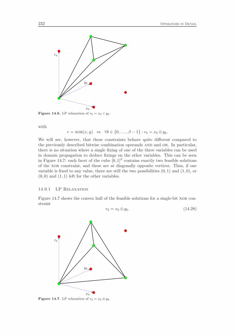
232 Operators in Detail
xb
yb
rb
Figure 14.6. LP relaxation of rb = xb ∨ yb.
withr = xor(x, y) ⇔ ∀b ∈ {0, . . . , β − 1} : rb = xb⊕ yb.
We will see, however, that these constraints behave quite different compared tothe previously described bitwise combination operands and and or. In particular,there is no situation where a single fixing of one of the three variables can be usedin domain propagation to deduce fixings on the other variables. This can be seenin Figure 14.7: each facet of the cube [0, 1]3 contains exactly two feasible solutionsof the xor constraint, and these are at diagonally opposite vertices. Thus, if onevariable is fixed to any value, there are still the two possibilities (0, 1) and (1, 0), or(0, 0) and (1, 1) left for the other variables.
14.9.1 LP Relaxation
Figure 14.7 shows the convex hull of the feasible solutions for a single-bit xor con-straint
rb = xb⊕ yb. (14.28)
xb
yb
rb
Figure 14.7. LP relaxation of rb = xb⊕ yb.

14.9. Bitwise Xor 233
Algorithm 14.15 Bitwise Xor Domain Propagation
Input : Bitwise xor constraint r = xor(x, y) on registers r, x, and y of widthβ with current local bit bounds lrb
≤ rb ≤ urb, lxb
≤ xb ≤ uxb, and
lyb≤ yb ≤ uyb
.
Output : Tightened local bounds for bits rb, xb, yb.
1. For all b = 0, . . . , β − 1:
(a) If two of the three bits in equation (14.28) are fixed, deduce the corres-ponding value for the remaining variable.
All of the four facets are non-trivial, i.e., they are not orthogonal to a unit vec-tor. Therefore, we need four “real” inequalities (as opposed to the bounds of thevariables) to describe the LP relaxation of the constraint:
rb − xb − yb ≤ 0
−rb + xb − yb ≤ 0
−rb − xb + yb ≤ 0
rb + xb + yb ≤ 2.
(14.29)
Each inequality cuts off one infeasible vertex of the unit cube. The first inequalitycuts off (1, 0, 0), the second (0, 1, 0), the third (0, 0, 1), and the fourth inequalitycuts off (1, 1, 1). Again, the LP relaxation (14.29) is “optimal” in the sense that itdescribes all facets of the convex hull of feasible solutions for the xor constraint.
14.9.2 Domain Propagation
As already mentioned, the domain propagation of the xor constraint is ratherweak. The value of a variable cannot be decided until all other variables are fixed.Therefore, the domain propagation consists of only one step, as depicted in Algo-rithm 14.15.
14.9.3 Presolving
The presolving of bitwise xor constraints is illustrated in Algorithm 14.16. Sincerb = xb⊕ yb ⇔ 0 = rb⊕xb⊕ yb, the resultant bit rb does not play a special role asin the and constraint. If any pair of variables is equivalent, the third variable canbe fixed to zero in Step 1a. On the other hand, if any pair of variables is negatedequivalent, the third variable can be fixed to one in Step 1b. If any of the bits isfixed to zero, the other two have to be equal and can be aggregated in Step 1c.Conversely, if any of the bits is fixed to one, the other two must be opposite andcan be aggregated accordingly in Step 1d. The domain propagation Algorithm 14.15does not need to be called since the deductions applied therein are already coveredby Steps 1c and 1d.
The presolving in Step 2 for pairs of constraints is slightly more involved thanthe one for bitwise and constraints. As before, we treat the constraints for each bitb in the form 0 = rb⊕xb⊕ yb and compare all pairs of those equations. If there aretwo pairs of equivalent or negated equivalent binary variables, the remaining pair ofvariables can be aggregated.

234 Operators in Detail
Algorithm 14.16 Bitwise Xor Presolving
1. For all active bitwise xor constraints r = xor(x, y):
(a) If rb⋆= xb, fix yb := 0.
If rb⋆= yb, fix xb := 0.
If xb⋆= yb, fix rb := 0.
(b) If rb Y⋆= xb, fix yb := 1.
If rb Y⋆= yb, fix xb := 1.
If xb Y⋆= yb, fix rb := 1.
(c) If rb = 0, aggregate xb : ⋆= yb.If xb = 0, aggregate rb : ⋆= yb.If yb = 0, aggregate rb : ⋆= xb.
(d) If rb = 1, aggregate xb : ⋆= 1− yb.If xb = 1, aggregate rb : ⋆= 1− yb.If yb = 1, aggregate rb : ⋆= 1− xb.
2. For all pairs of active bitwise xor constraints r = xor(x, y) and r′ =xor(x′, y′), including pairs with equal constraints, and all b = 0, . . . , βr − 1and b′ = 0, . . . , βr′ − 1:
If (ξ, ψ, ϕ) is any permutation of (rb, xb, yb), (ξ′, ψ′, ϕ′) is any permutation of(r′b, x
′b, y′b), and
(a) if ξ ⋆= ξ′ and ψ ⋆= ψ′, aggregate ϕ : ⋆= ϕ′,
(b) if ξ ⋆= ξ′ and ψ Y⋆= ψ′, aggregate ϕ : ⋆= 1− ϕ′,
(c) if ξ Y⋆= ξ′ and ψ Y
⋆= ψ′, aggregate ϕ : ⋆= ϕ′.
14.10 Unary And
The unary logic operators uand, uor, and uxor combine all bits of one register to calculate a single resultant bit. Thus, they are the first operators described herethat provide a link from multi-bit registers of the data path to single-bit registers ofthe control logic of a circuit. The uand constraint
uand : [β]→ [1], x 7→ r = uand(x)
is defined by
r = uand(x) ⇔ r = x0 ∧ . . . ∧ xβ−1.
As mentioned in Section 14.7, the binary bitwise and constraints are disaggregatedinto β single-bit constraints rb = xb ∧ yb. In this regard, the unary uand constraintis just a generalization of this single-bit equation to arbitrary many variables in theconjunction. In fact, in SCIP we only treat the general case
r = x0 ∧ . . . ∧ xk−1
of conjunctions of binary variables. The equations for the individual bits in a binarybitwise and constraint are just conjunctions with k = 2, while uand constraints areconjunctions with k = β. Therefore, the LP relaxation and the domain propagationand presolving algorithms of Section 14.7 are just special incarnations of the LPrelaxation and algorithms described below.

14.10. Unary And 235
Algorithm 14.17 Unary And Domain Propagation
Input : Unary and constraint r = uand(x) on single-bit register r and multi-bit register x of width β with current local bit bounds lr ≤ r ≤ ur andlxb≤ xb ≤ uxb
, b = 0, . . . , β − 1.
Output : Tightened local bounds for bits r and xb.
1. If uxb= 0 for any b ∈ {0, . . . , β − 1}, deduce r = 0.
2. If lxb= 1 for all b = 0, . . . , β − 1, deduce r = 1.
3. If lr = 1, deduce xb = 1 for all b = 0, . . . , β − 1.
4. If ur = 0 and lxb= 1 for all b 6= k, k ∈ {0, . . . , β − 1}, deduce xk = 0.
14.10.1 LP Relaxation
The LP relaxation of a uand constraint r = uand(x) can be stated as
r − xb ≤ 0 for all b = 0, . . . , β − 1 (14.30)
−r +
β−1∑
b=0
xb ≤ β − 1. (14.31)
The first inequality enforces the implication xb = 0→ r = 0 for all bits b, while thesecond inequality represents the implication (∀b : xb = 1)→ r = 1.
Lemma 14.25. The convex hull Puand = conv{(r, x) | r ∈ {0, 1}, x ∈ {0, 1}β, r =uand(x)} of the feasible solutions for the uand constraint is full-dimensional ifβ ≥ 2.
Proof. The feasible solutions (r = 0, x = 0), (r = 0, xb = 1, xi = 0 for i 6= b),b = 0, . . . , β − 1, and (r = 1, x = 1) define β + 2 affinely independent vectors inRβ+1. Thus, the dimension of Puand is dim(Puand) = β + 1.
Proposition 14.26. Inequalities (14.30) and (14.31) and the lower bound r ≥ 0define facets of Puand if β ≥ 2.
Proof. Puand is full-dimensional as shown in Lemma 14.25. Thus, it suffices foreach inequality to provide β + 1 affinely independent feasible solution vectors thatfulfill the inequality with equality. The solutions (r = 0, x = 0), (r = 0, xi =1, xj = 0 for j 6= i), i ∈ {0, . . . , β − 1} \ {b}, and (r = 1, x = 1) are affinelyindependent and fulfill inequality (14.30) for bit b with equality. The solutions(r = 0, xb = 0, xi = 1 for i 6= b), b = 0, . . . , β − 1, and (r = 1, x = 1) are also affinelyindependent and fulfill inequality (14.31) with equality. The solutions (r = 0, x = 0)and (r = 0, xb = 1, xi = 0 for i 6= b), b = 0, . . . , β − 1, are affinely independent andfulfill r ≥ 0 with equality.
14.10.2 Domain Propagation
The domain propagation Algorithm 14.17 is the canonical generalization of Algo-rithm 14.13. If a bit in the operand is zero, the resultant can be fixed to zero inStep 1. If all bits of the operand are one, the resultant must also be one, see Step 2.Conversely, if the resultant is fixed to one, all bits of the operand can be fixed to
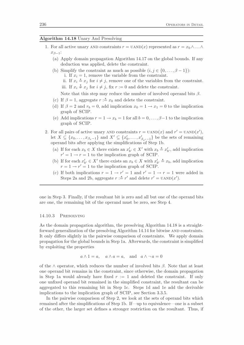
236 Operators in Detail
Algorithm 14.18 Unary And Presolving
1. For all active unary and constraints r = uand(x) represented as r = x0∧ . . .∧xβ−1:
(a) Apply domain propagation Algorithm 14.17 on the global bounds. If anydeduction was applied, delete the constraint.
(b) Simplify the constraint as much as possible (i, j ∈ {0, . . . , β − 1}):i. If xi = 1, remove the variable from the constraint.
ii. If xi⋆= xj for i 6= j, remove one of the variables from the constraint.
iii. If xi Y⋆= xj for i 6= j, fix r := 0 and delete the constraint.
Note that this step may reduce the number of involved operand bits β.
(c) If β = 1, aggregate r : ⋆= x0 and delete the constraint.
(d) If β = 2 and rb = 0, add implication x0 = 1→ x1 = 0 to the implicationgraph of SCIP.
(e) Add implications r = 1→ xb = 1 for all b = 0, . . . , β−1 to the implicationgraph of SCIP.
2. For all pairs of active unary and constraints r = uand(x) and r′ = uand(x′),let X ⊆ {x0, . . . , xβx−1} and X ′ ⊆ {x′0, . . . , x
′βx′−1} be the sets of remaining
operand bits after applying the simplifications of Step 1b.
(a) If for each xb ∈ X there exists an x′b′ ∈ X′ with xb
⋆= x′b′ , add implicationr′ = 1→ r = 1 to the implication graph of SCIP.
(b) If for each x′b′ ∈ X′ there exists an xb ∈ X with x′b′
⋆= xb, add implicationr = 1→ r′ = 1 to the implication graph of SCIP.
(c) If both implications r = 1 → r′ = 1 and r′ = 1 → r = 1 were added inSteps 2a and 2b, aggregate r : ⋆= r′ and delete r′ = uand(x′).
one in Step 3. Finally, if the resultant bit is zero and all but one of the operand bitsare one, the remaining bit of the operand must be zero, see Step 4.
14.10.3 Presolving
As the domain propagation algorithm, the presolving Algorithm 14.18 is a straight-forward generalization of the presolving Algorithm 14.14 for bitwise and constraints.It only differs slightly in the pairwise comparison of constraints. We apply domainpropagation for the global bounds in Step 1a. Afterwards, the constraint is simplifiedby exploiting the properties
a ∧ 1 = a, a ∧ a = a, and a ∧ ¬ a = 0
of the ∧ operator, which reduces the number of involved bits β. Note that at leastone operand bit remains in the constraint, since otherwise, the domain propagationin Step 1a would already have fixed r := 1 and deleted the constraint. If onlyone unfixed operand bit remained in the simplified constraint, the resultant can beaggregated to this remaining bit in Step 1c. Steps 1d and 1e add the derivableimplications to the implication graph of SCIP, see Section 3.3.5.
In the pairwise comparison of Step 2, we look at the sets of operand bits whichremained after the simplifications of Step 1b. If—up to equivalence—one is a subsetof the other, the larger set defines a stronger restriction on the resultant. Thus, if
14.11. Unary Or 237
the resultant for the larger set is one, then the other resultant must also be one. Ifboth sets are equal up to equivalence, the resultants can be aggregated and one ofthe constraints can be deleted.
14.11 Unary Or
The unary or constraint is defined similar to the unary and constraint as
uor : [β]→ [1], x 7→ r = uor(x)
withr = uor(x) ⇔ r = x0 ∨ . . . ∨ xβ−1.
By using the equivalence
r = x0 ∨ . . . ∨ xβ−1 ⇔ ¬ r = ¬x0 ∧ . . . ∧ ¬xβ−1
we can transform any uor constraint into an equivalent uand constraint. Thistransformation is applied in the presolving stage of SCIP. As already mentioned inSection 14.8, it is advantageous for the pairwise constraint comparison in the pre-solving algorithm to represent all and, or, uand, and uor constraints as constraintsof the same type.
14.12 Unary Xor
The unary exclusive or operator
uxor : [β]→ [1], x 7→ r = uxor(x)
withr = uxor(x) ⇔ r = x0⊕ . . .⊕xβ−1
is the generalization of equation (14.28) for the individual bits in a bitwise xorconstraint as discussed in Section 14.9. It inherits the poor domain propagationpotential of equation (14.28): a variable involved in a uxor constraint can onlybe fixed to a certain value after all other variables have been fixed. In contrastto the unary and and unary or constraints, the canonical LP relaxation of uxorconstraints consists of exponentially many inequalities. To avoid a blow-up of the LPrelaxation, we add an integer auxiliary variable, such that a single equation sufficesto model the uxor constraint. Unfortunately, this relaxation is almost useless if theintegrality of the auxiliary variable is not exploited by cutting planes, branching, orconflict analysis.
14.12.1 LP Relaxation
The number of inequalities in the LP relaxation of uand and uor constraints islinear in the number of operand bits β. Unfortunately, this is not true for uxorconstraints. Using the equivalence
r = x0⊕ . . .⊕xβ−1 ⇔ 0 = x0⊕ . . .⊕xβ−1 ⊕ r

238 Operators in Detail
and identifying xβ : ⋆= r, the LP relaxation of a uxor constraint can be stated as
∑
b∈S
xb −∑
b∈X\S
xb ≤ 2k for all k = 0, . . . ,⌊β
2
⌋, S ⊆ X with |S| = 2k + 1 (14.32)
with X = {0, . . . , β}. Here, each inequality cuts off only one of the infeasible {0, 1}-vectors, such that we need exponentially many inequalities. We cannot do betterwith inequalities defined in the space RX of problem variables, since all inequalitiesof type (14.32) represent facets of the convex hull
Puxor = conv{(r, x) ∈ {0, 1}X | r = uxor(x)
}
of integer points that satisfy the constraint:
Lemma 14.27. The convex hull Puxor of the feasible solutions for the uxor con-straint is full-dimensional if β ≥ 2.
Proof. The feasible solutions (r = 0, x = 0), (r = 1, xb = 1, xi = 0 for i 6= b),b = 0, . . . , β − 1, and (r = 0, x0 = 1, x1 = 1, xb = 0 for b = 2, . . . , β − 1) define β + 2affinely independent vectors in Rβ+1. Thus, the dimension of Puxor is dim(Puxor) =β + 1.
Proposition 14.28. Each inequality (14.32) defines a facet of Puxor if β ≥ 2. Thebounds xb ≥ 0 and xb ≤ 1 define facets of Puxor for all b ∈ X if β ≥ 3.
Proof. Puxor is full-dimensional as shown in Lemma 14.27. Thus, it suffices foreach inequality to provide β+1 affinely independent solution vectors that fulfill theinequality with equality.
Let k ∈{0, . . . , ⌊β
2⌋}
and S ⊆ X with |S| = 2k + 1. For β ≥ 2, the vectors
xb = (xbi)i=0,...,β with xb
i =
{
1 if i ∈ S \ {b}
0 otherwise,
b = 0, . . . , β, are β + 1 affinely independent solutions of 0 = x0⊕ . . .⊕xβ thatfulfill inequality (14.32) for the given k and S with equality. For β ≥ 3, the vector(0, . . . , 0), the vectors
xb = (xbi)i=0,...,β with xb
i =
{
1 if i ∈ {1, b}
0 otherwise,
b = 2, . . . , β, and the vector (0, . . . , 0, 1, 1) are β + 1 affinely independent solutionsof 0 = x0⊕ . . .⊕xβ that fulfill the lower bound x0 ≥ 0 with equality. For β ≥ 3,the upper bound x0 ≤ 1 is fulfilled with equality by the β + 1 affine independentsolution vectors
xb = (xbi)i=0,...,β with xb
i =
{
1 if i ∈ {0, b}
0 otherwise,
b = 1, . . . , β and (1, 1, 1, 1, 0, . . . , 0). If β ≥ 3, the other bounds are facets foranalogous reasons.
Corollary 14.29. The number of facets of the convex hull Puxor of feasible solutionsof the uxor constraint is exponential in the number of variables.

14.12. Unary Xor 239
Algorithm 14.19 Unary Xor Domain Propagation
Input : Unary xor constraint r = uxor(x) on single-bit register r and multi-bit register x of width β with current local bit bounds lr ≤ r ≤ ur andlxb≤ xb ≤ uxb
, b = 0, . . . , β − 1.
Output : Tightened local bounds for bits r and xb.
1. If all variables except one are fixed, deduce the corresponding value for theremaining variable.
In order to avoid the exponential blow-up of the LP relaxation, we use sys-tem (14.32) only if β = 2. Otherwise, we introduce an auxiliary integer variableq ∈
{0, . . . , ⌈β
2⌉}
and state by the single equation
r + x0 + . . . + xβ−1 = 2q (14.33)
that the number of variables set to one in an uxor constraint must be even. Thedisadvantage of equation (14.33) and the introduction of the auxiliary variable q isthat this LP relaxation is much weaker than the exponentially large system (14.32).For example, in the case β = 2, the polyhedron defined by equation (14.33) and thebounds of the variables has the vertices
(r, x0, x1, q) ∈{(0, 0, 0, 0), (0, 1, 1, 1), (1, 0, 1, 1), (1, 1, 0, 1),
(0, 0, 1, 0.5), (0, 1, 0, 0.5), (1, 0, 0, 0.5)}
with the last three being invalid solutions of the constraint. Without enforcing theintegrality of q, the LP relaxation 14.33 is almost useless. However, it may becomeuseful during the course of the solution process, if q starts to appear in cutting planesor conflict constraints or if it is selected as branching variable.
14.12.2 Domain Propagation
As already mentioned above, we only apply a single type of propagation to uxorconstraints: if all but one of the variables are fixed, we can deduce the correspondingvalue for the remaining variable. This procedure is depicted in Algorithm 14.19,which is a generalization of the propagation Step 1a of Algorithm 14.15.
14.12.3 Presolving
The presolving of unary xor constraints is illustrated in Algorithm 14.20. It isa generalization of Algorithm 14.16 to exclusive disjunctions with arbitrary manyaddends. In Step 1a we simplify the constraint by removing variables fixed to zeroand pairs of equivalent or negated equivalent variables, exploiting the properties
a⊕ 0 = a, a⊕ a = 0, and a⊕¬ a = 1
of the ⊕ operator. The “⊕ 1” addends appended by rule 1(a)iii are treated likevariables which are fixed to one. Thus, if there exists another variable fixed toone in the constraint or if rule 1(a)iii is applied multiple times, the “⊕ 1” addendscancel each other by rule 1(a)ii. Thus, at most one fixed variable remains in the
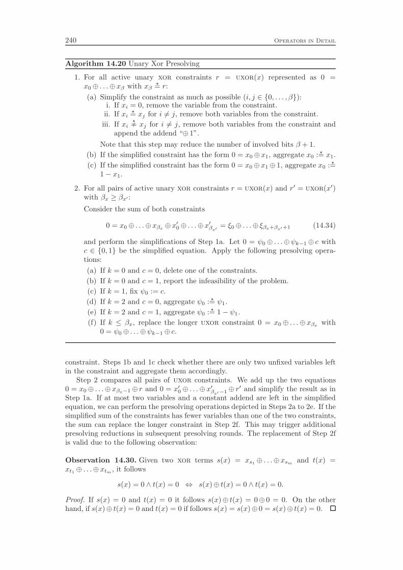
240 Operators in Detail
Algorithm 14.20 Unary Xor Presolving
1. For all active unary xor constraints r = uxor(x) represented as 0 =x0⊕ . . .⊕xβ with xβ
⋆= r:
(a) Simplify the constraint as much as possible (i, j ∈ {0, . . . , β}):i. If xi = 0, remove the variable from the constraint.
ii. If xi⋆= xj for i 6= j, remove both variables from the constraint.
iii. If xi Y⋆= xj for i 6= j, remove both variables from the constraint and
append the addend “⊕ 1”.
Note that this step may reduce the number of involved bits β + 1.
(b) If the simplified constraint has the form 0 = x0⊕x1, aggregate x0 : ⋆= x1.
(c) If the simplified constraint has the form 0 = x0⊕ x1⊕ 1, aggregate x0 : ⋆=1− x1.
2. For all pairs of active unary xor constraints r = uxor(x) and r′ = uxor(x′)with βx ≥ βx′ :
Consider the sum of both constraints
0 = x0⊕ . . .⊕xβx⊕x′0⊕ . . .⊕x
′βx′
= ξ0⊕ . . .⊕ ξβx+βx′+1 (14.34)
and perform the simplifications of Step 1a. Let 0 = ψ0⊕ . . .⊕ψk−1⊕ c withc ∈ {0, 1} be the simplified equation. Apply the following presolving opera-tions:
(a) If k = 0 and c = 0, delete one of the constraints.
(b) If k = 0 and c = 1, report the infeasibility of the problem.
(c) If k = 1, fix ψ0 := c.
(d) If k = 2 and c = 0, aggregate ψ0 : ⋆= ψ1.
(e) If k = 2 and c = 1, aggregate ψ0 : ⋆= 1− ψ1.
(f) If k ≤ βx, replace the longer uxor constraint 0 = x0⊕ . . .⊕xβxwith
0 = ψ0⊕ . . .⊕ψk−1⊕ c.
constraint. Steps 1b and 1c check whether there are only two unfixed variables leftin the constraint and aggregate them accordingly.
Step 2 compares all pairs of uxor constraints. We add up the two equations0 = x0⊕ . . .⊕ xβx−1⊕ r and 0 = x′0⊕ . . .⊕x
′βx′−1⊕ r
′ and simplify the result as inStep 1a. If at most two variables and a constant addend are left in the simplifiedequation, we can perform the presolving operations depicted in Steps 2a to 2e. If thesimplified sum of the constraints has fewer variables than one of the two constraints,the sum can replace the longer constraint in Step 2f. This may trigger additionalpresolving reductions in subsequent presolving rounds. The replacement of Step 2fis valid due to the following observation:
Observation 14.30. Given two xor terms s(x) = xs1⊕ . . .⊕ xsm
and t(x) =xt1 ⊕ . . .⊕ xtm
, it follows
s(x) = 0 ∧ t(x) = 0 ⇔ s(x)⊕ t(x) = 0 ∧ t(x) = 0.
Proof. If s(x) = 0 and t(x) = 0 it follows s(x)⊕ t(x) = 0⊕ 0 = 0. On the otherhand, if s(x)⊕ t(x) = 0 and t(x) = 0 if follows s(x) = s(x)⊕ 0 = s(x)⊕ t(x) = 0.
14.13. Equality 241
14.13 Equality
The equality operator
eq : [β]× [β]→ [1], (x, y) 7→ r = eq(x, y)
withr = eq(x, y) ⇔ r ↔ (x = y)
provides a very important link from the data path to the control logic of the circuit.Often, x and y are results of some arithmetic computations, and the behavior of thecontrol logic depends on whether the two results are equal or not.
Many property checking problems are modeled like Example 13.2, where theoutput of a copy of the circuit with different input assignments is compared to theoutput of the original circuit by an equality constraint. Other common propertiescompare the circuit with a reference implementation and check whether the twooutputs are always equal. In both cases, the property states that equality of theoutputs must hold. This means, that in the corresponding CIP model which includesthe negated property, the resultant of the equality constraint is fixed to zero, andwe search for a counter-example where the outputs are unequal. Unfortunately, thedomain propagation behavior of eq constraints is much worse for r = 0 than for r =1, see Section 14.13.2. The same holds for presolving as discussed in Section 14.13.3.If the resultant is fixed to r = 1, we can apply pairwise aggregation of the bits inthe two operands and delete the constraint from the model. For r = 0, we can onlyconclude that x Y
⋆= y, which is a very weak information.
The LP relaxation is defined on word level and contains a number of auxiliaryvariables. Additionally, two “big-M” coefficients are included with values up to 2W ,with W = 16 being the width of the words.
14.13.1 LP Relaxation
We use an LP relaxation of the constraint r = eq(x, y) on the word level which usesfour auxiliary variables sw, tw ∈ Z≥0, and pw, qw ∈ {0, 1} per word:
xw − yw = sw − tw for all w = 0, . . . , ω − 1 (14.35)
sw ≤ (uxw − lyw ) · pw for all w = 0, . . . , ω − 1 (14.36)
tw ≤ (uyw − lxw ) · qw for all w = 0, . . . , ω − 1 (14.37)
pw − sw ≤ 0 for all w = 0, . . . , ω − 1 (14.38)
qw − tw ≤ 0 for all w = 0, . . . , ω − 1 (14.39)
r + pw + qw ≤ 1 for all w = 0, . . . , ω − 1 (14.40)
r +ω−1∑
w=0
(pw + qw) ≥ 1 (14.41)
If ω = 1, we can replace (14.40) and (14.41) by the equation r + p0 + q0 = 1.Equation (14.35) splits the difference xw − yw into the positive part sw and
the negative part tw. The binary variable pw should be one if and only if sw > 0which means xw > yw. The binary variable qw should be one if and only if tw >0 which means xw < yw. Thus, the variables pw and qw reflect the sign of thedifference xw − yw. These relations are ensured by inequalities (14.36) to (14.39).Inequality (14.36) models the implication pw = 0 → sw = 0. Inequality (14.37)
242 Operators in Detail
ensures qw = 0 → tw = 0. Both inequalities are redundant for pw = 1 or qw = 1,respectively. Inequalities (14.38) and (14.39) model pw = 1→ sw ≥ 1 and qw = 1→tw ≥ 1. The last inequality (14.40) introduced for all words w ensures that at mostone of sw and tw can be positive, and if r = 1 both have to be zero, which meansthat xw = yw. Finally, the single inequality (14.41) reflects the opposite implication(∀w : xw = yw)→ r = 1.
14.13.2 Domain Propagation
As already noted in the introduction of this section, the domain propagation of theequality constraint is very unbalanced comparing the cases that r is fixed to zeroor one. In the case r = 1, we can immediately conclude that each pair of bits xb
and yb in the operators must have the same value, i.e., xb = yb. If one of the bits isfixed, we can deduce the corresponding value for the other bit. In the case r = 0,however, we can conclude almost nothing. Only if for all pairs except one the bitshave the same value and one variable of the remaining pair is already fixed, we canconclude that the other variable must take the opposite value in order to enforce theinequality of the two registers.
In the other direction, we can conclude r = 0 immediately after a bit pair withopposite values is detected. The deduction of r = 1 can only be carried out if alloperand bits are fixed to pairwise equal values.
Algorithm 14.21 illustrates this procedure. Step 1a implements the implicationr = 1 → ∀b : xb = yb, while Step 1b propagates the implication in the oppositedirection (∃b : xb 6= yb)→ r = 0. Steps 2 and 3 apply the very weak deduction rules(∀b : xb = yb)→ r = 1 and r = 0→ ∃b : xb 6= yb, respectively.
The auxiliary variables are propagated in Steps 4 to 6. If the resultant is fixedto r = 1, we can fix all sign variables pw and qw to zero in Step 4a. If one ofthe sign variables is fixed for an individual word w, we can apply the correspondingdeductions in Step 4b. Propagating the bounds on tw = yw−xw means to iterativelytighten the bounds of the variables by
lyw − uxw ≤ tw ≤ uyw − lxw
lyw − utw ≤ xw ≤ uyw − ltw
ltw + lxw ≤ yw ≤ utw + uxw
as long as no more bounds can be tightened or an infeasibility is detected. If weknow that one of the variables sw or tw is either zero or non-zero, we can drawthe appropriate conclusions on the sign variables in Step 4c. Note that afterwardsadditional deductions are performed in the next iteration in Step 4b. From the lowerand upper bounds of the word variables xw and yw, we can also deduce fixings ofpw and qw as shown in Step 4d. We could already tighten the lower bounds of sw
and tw, but this will automatically happen in Step 4b of the next iteration of thedomain propagation loop. The upper bounds of sw and tw, however, are tightenedin Step 4e.
If the sign variables pw and qw are zero for all words, we can deduce r = 1.Note that this deduction does not automatically follow from rules 4b and 2, becausealthough we already know that sw = tw = 0 in Step 4b, we usually cannot fix thebounds of xw and yw to a specific value which is necessary to deduce fixings of thebit variables in the domain propagation Algorithm 14.1 of the bit/word partitioningconstraints. Finally in Step 6, if the sign variables pw and qw are zero for all words

14.13. Equality 243
Algorithm 14.21 Equality Domain Propagation
Input : Equality constraint r = eq(x, y) on single-bit register r and multi-bit reg-isters x and y of width β with current local bit bounds lr ≤ r ≤ ur,lxb≤ xb ≤ uxb
, and lyb≤ yb ≤ uyb
, b = 0, . . . , β − 1; current local bounds
on auxiliary variables lsw ≤ sw ≤ usw , ltw ≤ tw ≤ utw , lpw ≤ pw ≤ upw ,
and lqw ≤ qw ≤ uqw , w = 0, . . . , ω − 1.
Output : Tightened local bounds for bits r, xb, yb, and auxiliary variables sw, tw,pw, and qw.
1. For all b = 0, . . . , β − 1:
(a) If lr = 1 and uxb= 0, deduce y = 0.
If lr = 1 and lxb= 1, deduce y = 1.
If lr = 1 and uyb= 0, deduce x = 0.
If lr = 1 and lyb= 1, deduce x = 1.
(b) If uxb= 0 and lyb
= 1, deduce r = 0.
If lxb= 1 and uyb
= 0, deduce r = 0.
2. If for all bits b ∈ {0, . . . , β− 1} we have uxb= uyb
= 0 or lxb= lyb
= 1, deducer = 1.
3. If for all bits b ∈ {0, . . . , β − 1} \ {k} we have uxb= uyb
= 0 or lxb= lyb
= 1,and if ur = 0, and
(a) if lxk= 1, deduce yk = 0,
(b) if uxk= 0, deduce yk = 1,
(c) if lyk= 1, deduce xk = 0,
(d) if uyk= 0, deduce xk = 1.
4. For all w = 0, . . . , ω − 1:
(a) If lr = 1, deduce pw = 0 and qw = 0.
(b) If lpw = 1, deduce r = 0, qw = 0, and sw ≥ 1.
If lqw = 1, deduce r = 0, pw = 0, and tw ≥ 1.If upw = 0, deduce sw = 0 and propagate bounds on tw = yw − xw.If uqw = 0, deduce tw = 0 and propagate bounds on sw = xw − yw.
(c) If lsw ≥ 1, deduce pw = 1.If ltw ≥ 1, deduce qw = 1.If usw = 0, deduce pw = 0.If utw = 0, deduce qw = 0.
(d) If lxw > uyw , deduce pw = 1.
If lxw ≥ uyw , deduce qw = 0.
If uxw < lyw , deduce qw = 1.
If uxw ≤ lyw , deduce pw = 0.
(e) Tighten bounds sw ≤ uxw − lyw and tw ≤ uyw − lxw .
5. If upw = uqw = 0 for all w ∈ {0, . . . , ω − 1}, deduce r = 1.
6. If upw = uqw = 0 for all w ∈ {0, . . . , ω − 1} \ {k} and ur = 0, and
(a) if upk = 0, deduce qk = 1,
(b) if uqk = 0, deduce pk = 1.
244 Operators in Detail
except word k, but the resultant is fixed to r = 0, we can propagate the equationpk + qk = 1, since one of the two variables must be non-zero.
14.13.3 Presolving
The presolving of equality constraints suffers from the same limitations as the domainpropagation. If the resultant r is fixed to one, we can aggregate all pairs of bits, butif the resultant is fixed to zero, we usually cannot apply any problem reductions.
Algorithm 14.22 shows the presolving steps that are performed on equality con-straints. If the resultant bit is one, we can aggregate the bits of the operandsaccordingly in Step 1b. Conversely, if the operands are equivalent, the resultant isfixed to one in Step 1c. In both cases the equality constraint becomes redundantand can be deleted.
In the opposite situation of r = 0, we can conclude that the operands cannot beequal. Therefore, we add in Step 1d each operand to the list of unequal registersof the other operand, see Section 14.1.4. On the other hand, if we know that theoperand registers cannot be equal because they appear in each other’s list of unequalregisters, we can fix r = 0 in Step 1e. Note that in both cases the constraintcannot be deleted, since the inequality x Y
⋆= y of registers is only an information
stored in the register data structures. The inequality is not enforced automaticallyduring the solving process. In particular, the constraint itself may have detected theinequality and has to be kept active in order to enforce the inequality. In contrast, theequivalence of registers means that the bits are pairwise aggregated in the variableaggregation graph of SCIP, see Section 3.3.4. Thus, they are represented in allother constraints by a unique representative, and the deletion of the constraint inSteps 1b and 1c is valid, since the whole information of the constraint is capturedby the aggregations.
Step 1f is a special case of Step 1e where the inequality of the operands is provenby a pair of bits that are negated equivalent, i.e., for which the equivalence xb
⋆= 1−yb
is stored in the variable aggregation tree. In this case, we can delete the constraintin addition to fix r := 0.
Step 1g is similar to Step 3 of the domain propagation Algorithm 14.21. If thereis only one bit pair k for which equivalence was not detected, and if one of theremaining three variables r, xk, and yk is fixed, we can aggregate the other twovariables accordingly. Of course, we do not need to treat the fixing r = 1, becausethis is already captured by Step 1b.
Step 1h corresponds to Step 6 of the domain propagation Algorithm 14.21. Ifthere is only one word k for which the sign variables pw and qw are not fixed tozero, two of the three variables r, pk, and qk can be aggregated, if the third variableis fixed to zero. Note that we cannot delete the constraint, since the link of theauxiliary variables pk and qk to the external variables xw and yw has still to beenforced.
For each fixed operand bit, we can add an implication to the implication graphof SCIP in Step 1i which states that if the other operand’s bit takes the oppositevalue, the resultant must be zero.
Pairs of equality constraints are processed in Step 2. If each pair of bits {x′b′ , y′b′}
of constraint r′ = eq(x′, y′) appears also as bit pair or as negated bit pair in con-straint r = eq(x, y), the equality of x and y implies the equality of x′ and y′.Therefore, we can in this case derive the implication r = 1 → r′ = 1 in Step 2a.If this is detected with interchanged roles of the constraints, the corresponding im-

14.13. Equality 245
Algorithm 14.22 Equality Presolving
1. For all active equality constraints r = eq(x, y):
(a) Apply domain propagation Algorithm 14.21 on the global bounds.
(b) If r = 1, aggregate x : ⋆= y and delete the constraint.
(c) If x ⋆= y, fix r := 1 and delete the constraint.
(d) If r = 0, deduce x Y⋆= y.
(e) If x Y⋆= y, fix r := 0.
(f) If for any bit b ∈ {0, . . . , β− 1} we have xb Y⋆= yb, fix r := 0 and delete the
constraint.
(g) If for all bits b ∈ {0, . . . , β − 1} \ {k} we have xb⋆= yb, and
i. if r = 0, aggregate xk : ⋆= 1− yk and delete the constraint,ii. if xk = 0, aggregate r : ⋆= 1− yk and delete the constraint,iii. if xk = 1, aggregate r : ⋆= yk and delete the constraint,iv. if yk = 0, aggregate r : ⋆= 1− xk and delete the constraint,v. if yk = 1, aggregate r : ⋆= xk and delete the constraint.
(h) If for all words w ∈ {0, . . . , ω − 1} \ {k} we have pw = qw = 0, andi. if r = 0, aggregate pk : ⋆= 1− qk,
ii. if pk = 0, aggregate r : ⋆= 1− qk,iii. if qk = 0, aggregate r : ⋆= 1− pk.
(i) For all b = 0, . . . , β − 1:i. If xb = 0, add implication yb = 1→ r = 0 to the implication graph.
ii. If xb = 1, add implication yb = 0→ r = 0 to the implication graph.iii. If yb = 0, add implication xb = 1→ r = 0 to the implication graph.iv. If yb = 1, add implication xb = 0→ r = 0 to the implication graph.
2. For all pairs of active equality constraints r = eq(x, y) and r′ = eq(x′, y′)with βx ≥ βx′ :
(a) If for all b′ ∈ {0, . . . , βx′ − 1} there exists b ∈ {0, . . . , βx − 1} such thati. xb
⋆= x′b′ and yb⋆= y′b′ , or
ii. xb⋆= y′b′ and yb
⋆= x′b′ , or
iii. xb Y⋆= x′b′ and yb Y
⋆= y′b′ , or
iv. xb Y⋆= y′b′ and yb Y
⋆= x′b′ ,
add the implication r = 1→ r′ = 1 to the implication graph of SCIP.
(b) If for all b ∈ {0, . . . , βx− 1} there exists b′ ∈ {0, . . . , βx′ − 1} such that atleast one of 2(a)i to 2(a)iv holds, add the implication r′ = 1 → r = 1 tothe implication graph of SCIP.
(c) If both Steps 2a and 2b were successfully applied, aggregate r : ⋆= r′ anddelete the constraint r = eq(x, y).
(d) If x ⋆= x′ and r Y⋆= r′, deduce y Y
⋆= y′.
If x ⋆= y′ and r Y⋆= r′, deduce y Y
⋆= x′.
If y ⋆= x′ and r Y⋆= r′, deduce x Y
⋆= y′.
If y ⋆= y′ and r Y⋆= r′, deduce x Y
⋆= x′.
(e) If x ⋆= x′ and y Y⋆= y′, add r = 1→ r′ = 0 to the implication graph.
If x ⋆= y′ and x Y⋆= y′, add r = 1→ r′ = 0 to the implication graph.
If x Y⋆= x′ and y ⋆= y′, add r = 1→ r′ = 0 to the implication graph.
If x Y⋆= y′ and y ⋆= x′, add r = 1→ r′ = 0 to the implication graph.
246 Operators in Detail
plication is added to the implication graph of SCIP in Step 2b. Having detectedboth implications for a pair of constraints means that the resultants are equivalent.Consequently, one of the constraints can be deleted in Step 2c.
Steps 2d and 2e exploit our knowledge about the inequality of registers. If oneof the operand in the first constraint is equivalent to an operand of the secondconstraint, but the resultants are negated equivalent, the remaining operand pairmust be unequal, which is detected in Step 2d. Conversely, if one pair of operandsis equivalent but the other pair of operands is unequal, we can conclude in Step 2ethat at least one of the resultants must be zero.
14.14 Less-Than
Like the equality constraint, the less-than operator
lt : [β]× [β]→ [1], (x, y) 7→ r = lt(x, y)
defined by
r = lt(x, y) ⇔ r ↔ (x < y)
provides a link from the data path to the control logic of the circuit. By negating theresultant and exchanging the operands, one can also model the other three inequalityoperands:
not(r) = lt(y, x) ⇔ r ↔ (x ≤ y)
r = lt(y, x) ⇔ r ↔ (x > y)
not(r) = lt(x, y) ⇔ r ↔ (x ≥ y)
Although the LP relaxation of lt constraints is very similar to the relaxation ofeq constraints, the domain propagation behavior of the less-than operator is evenworse than the one of the equality operator. The propagation performance of afixed resultant value is symmetric in lt constraints: in both cases, we usually cannot deduce anything. The same holds for presolving. Due to the transitivity of the< operator, however, we have additional possibilities to discover inequality relationsbetween registers in the pairwise comparison of lt constraints.
14.14.1 LP Relaxation
The LP relaxation for less-than constraints r = lt(x, y) differs only slightly fromthe relaxation of eq constraints. It is also defined on the word level and uses four
14.14. Less-Than 247
auxiliary variables sw, tw ∈ Z≥0, and pw, qw ∈ {0, 1} per word:
xw − yw = sw − tw for all w = 0, . . . , ω − 1 (14.42)
sw ≤ (uxw − lyw ) · pw for all w = 0, . . . , ω − 1 (14.43)
tw ≤ (uyw − lxw ) · qw for all w = 0, . . . , ω − 1 (14.44)
pw − sw ≤ 0 for all w = 1, . . . , ω − 1 (14.45)
qw − tw ≤ 0 for all w = 0, . . . , ω − 1 (14.46)
pw + qw ≤ 1 for all w = 1, . . . , ω − 1 (14.47)
p0 + q0 = 1 (14.48)
r + pw −ω−1∑
k=w+1
qk ≤ 1 for all w = 0, . . . , ω − 1 (14.49)
−r + qw −ω−1∑
k=w+1
pk ≤ 0 for all w = 0, . . . , ω − 1 (14.50)
As before, constraints (14.42) to (14.47) split the difference xw−yw into the positivepart sw and the negative part tw with pw = 1 if and only if xw > yw and qw = 1 ifand only if xw < yw (with a slight deviation for the least significant word w = 0, seebelow). As opposed to the equality constraint, the position of the operand wordsplay an important role: a less significant word can only influence the resultant, ifall more significant words of x and y are pairwise equal. Therefore, the resultant ris not necessarily affected by all words and does not appear in inequality (14.47).Instead, the significance of the words and their relation to the resultant is capturedby inequalities (14.49) and (14.50). For the most significant word w = ω − 1, thesums are empty and the inequalities are reduced to
r + pω−1 ≤ 1 and − r + qω−1 ≤ 0,
which model the valid implications pω−1 = 1 → r = 0 and qω−1 = 1 → r = 1,respectively. Only if pω−1 = qω−1 = 0, i.e., xω−1 = yω−1, the value of the resultantis determined by the lower significant words. Thus, we had to include the sums intoinequalities (14.49) and (14.50) to render them redundant whenever the resultantis already determined on higher significant words. Altogether, inequality (14.49)represents the implication
(∀k > w : qk = 0) ∧ pw = 1→ r = 0,
and inequality (14.50) models
(∀k > w : pk = 0) ∧ qw = 1→ r = 1
for words w = 0, . . . , ω − 1.
The least significant word w = 0 plays a slightly different role than the otherwords. The equality x0 = y0 is, with respect to the value of the resultant, equivalentto x0 > y0: in both cases the resultant is zero if all more significant words arepairwise equal. Therefore, we define p0 to be one if and only if x0 ≥ y0, in contrast toxw > yw for the other words. This turns inequality (14.47) into the equation (14.48)and makes inequality (14.45) invalid for word w = 0. Of course, we can immediatelyaggregate p0 : ⋆= 1− q0 and replace the occurrences of p0 accordingly.
248 Operators in Detail
14.14.2 Domain Propagation
The domain propagation for less-than constraints is depicted in Algorithm 14.23.Steps 1 and 2 apply domain propagation on the bits of the operand registers x andy. We iterate over the bits from most significant to least significant bit, since lesssignificant bits might be irrelevant if the value of the resultant is already determinedby the more significant bits.
If we know that in the current local bounds xb < yb holds for a bit b and ifxj ≤ yj for all higher significant bits j > b, the fixings at bit b prove that x < y,and we can deduce r = 1 in Step 1a. Conversely, if for a bit b we have xb > yb andxj ≥ yj for all j > b, it clearly follows x > y and thus r = 0, which is deduced inStep 1b.
Steps 1c and 1d apply this reasoning in the other way. If we already know thatr = 1 but there is a bit b with xb > yb and we have xj ≥ yj for all more significantbits j > b except for a single bit k, we can conclude in Step 1c that the inequalityx < y must hold due to bit k. Thus, it follows xk < yk which means xk = 0 andyk = 1. On the other hand, if we know that r = 0 but xb < yb for a bit b withxj ≤ yj for all j > b except for bit k, we can deduce xk > yk, i.e., xk = 1 and yk = 0in Step 1d.
If r = 1 but for the highest significant bits j ≥ b we have xj ≥ yj , it must bexj = yj for all j ≥ b. This deduction is iteratively applied at Step 1e while the bitsare scanned from b = β− 1 down to b = 0, such that we only need to fix the currentbits xb and yb. Conversely, if r = 0 but xj ≤ yj for all j ≥ b, we can concludexj = yj for all j ≥ b in Step 1f.
If we detected during the loop of Step 1 that xb ≥ yb for all bits, we have x ≥ yand can conclude r = 0 in Step 2.
Steps 3 and 4 propagate the auxiliary variables for the operand words. Again,we iterate from most significant to least significant word. Steps 3a to 3f are verysimilar to the bit level propagations of Step 1. If for a word w we have qw = 1 andpj = 0 for all j > w, we know that xw < yw and xj ≤ yj for all j > w. It followsx < y and thus r = 1, which is deduced in Step 3a. Conversely, if pw = 1 and qj = 0for all j > w, we have x > y (or x ≥ y if w = 0) and we can conclude r = 0 inStep 3b. If we know that r = 1 but pw = 1 and qj = 0 for all words j > w exceptword k, it must be qk = 1, which is deduced in Step 3c. On the other hand, if r = 0but qw = 1 and pj = 0 for all words j > w except word k, we can conclude pk = 1in Step 3d. If r = 1 and qj = 0 for all j ≥ w, it must also be pj = 0 for all j ≥ w.This deduction is performed successively in Step 3e. Step 3f applies the oppositepropagation: if r = 0 and pj = 0 for all j ≥ w, it follows qj = 0 for all j ≥ w.
Steps 3g to 3j apply the same reasoning as Steps 4b to 4e of the domain prop-agation Algorithm 14.21 for equality constraints, except that the different meaningof p0 must be regarded. Finally, if in the loop of Step 3 we detected qw = 0 for allwords w, we can conclude r = 0 in Step 4.
14.14.3 Presolving
The presolving Algorithm 14.24 for less-than constraints does not consist of muchmore than to call the domain propagation on the global bounds in Step 1a. However,if a propagation on the external variables was applied that completely determinedthe status of the constraint, we can delete the constraint from the model. If theoperands are equivalent, we can clearly deduce r = 0 in Step 1b and delete theconstraint. If on the other hand, the resultant is fixed to r = 1 in Step 1c, the

14.14. Less-Than 249
Algorithm 14.23 Less-Than Domain Propagation
Input : Less-than constraint r = lt(x, y) on single-bit register r and multi-bitregisters x and y of width β with current local bit bounds lr ≤ r ≤ ur,lxb≤ xb ≤ uxb
, and lyb≤ yb ≤ uyb
, b = 0, . . . , β − 1; current local bounds
on auxiliary variables lsw ≤ sw ≤ usw , ltw ≤ tw ≤ utw , lpw ≤ pw ≤ upw ,
and lqw ≤ qw ≤ uqw , w = 0, . . . , ω − 1.
Output : Tightened local bounds for bits r, xb, yb, and auxiliary variables sw, tw,pw, and qw.
1. For all b = β − 1, . . . , 0:
(a) If uxb= 0, lyb
= 1, and uxj≤ lyj
for all j > b, deduce r = 1.
(b) If lxb= 1, uyb
= 0, and lxj≥ uyj
for all j > b, deduce r = 0.
(c) If lr = 1, lxb= 1, uyb
= 0, and lxj≥ uyj
for all j ∈ {b+1, . . . , β−1}\{k},deduce xk = 0 and yk = 1.
(d) If ur = 0, uxb= 0, lyb
= 1, and uxj≤ lyj
for all j ∈ {b+1, . . . , β−1}\{k},deduce xk = 1 and yk = 0.
(e) If lr = 1, and lxj≥ uyj
for all j ≥ b, deduce xb ≤ uyband yb ≥ lxb
.
(f) If ur = 0, and uxj≤ lyj
for all j ≥ b, deduce xb ≥ lyband yb ≤ uxb
.
2. If lxb≥ uyb
for all b = 0, . . . , β − 1, deduce r = 0.
3. For all w = ω − 1, . . . , 0:
(a) If lqw = 1 and upj = 0 for all j > w, deduce r = 1.
(b) If lpw = 1 and uqj = 0 for all j > w, deduce r = 0.
(c) If lr = 1, lpw = 1, and uqj = 0 for all j ∈ {w+1, . . . , ω− 1} \ {k}, deduceqk = 1.
(d) If lr = 0, lqw = 1, and upj = 0 for all j ∈ {w+1, . . . , ω− 1} \ {k}, deducepk = 1.
(e) If lr = 1, and uqj = 0 for all j ≥ w, deduce pw = 0.
(f) If lr = 0, and upj = 0 for all j ≥ w, deduce qw = 0.
(g) If lpw = 1, deduce qw = 0, and if additionally w ≥ 1, deduce sw ≥ 1.
If lqw = 1, deduce pw = 0 and tw ≥ 1.If upw = 0, deduce sw = 0 and propagate bounds on tw = yw − xw.If uqw = 0, deduce tw = 0 and propagate bounds on sw = xw − yw.
(h) If lsw ≥ 1, deduce pw = 1.If ltw ≥ 1, deduce qw = 1.If usw = 0 and w ≥ 1, deduce pw = 0.If utw = 0, deduce qw = 0.
(i) If lxw > uyw , deduce pw = 1.
If lxw ≥ uyw , deduce qw = 0.
If uxw < lyw , deduce qw = 1.
If uxw ≤ lyw and w ≥ 1, deduce pw = 0.
(j) Tighten bounds sw ≤ uxw − lyw and tw ≤ uyw − lxw .
4. If uqw = 0 for all w = 0, . . . , ω − 1, deduce r = 0.
250 Operators in Detail
Algorithm 14.24 Less-Than Presolving
1. For all active less-than constraints r = lt(x, y):
(a) Apply domain propagation Algorithm 14.23 on the global bounds. If anyof rules 1a to 1d or rule 2 was applied, delete the constraint.
(b) If x ⋆= y, fix r := 0 and delete the constraint.
(c) If r = 1, deduce x Y⋆= y.
(d) For all b = β − 1, . . . , 0:If xj
⋆= yj for all j ∈ {b+ 1, . . . , β − 1} \ {k}, andi. if xb = 0, yb = 1, and xk = 1, aggregate r : ⋆= yk,
ii. if xb = 0, yb = 1, and yk = 0, aggregate r : ⋆= 1− xk.iii. if xb = 1, yb = 0, and xk = 0, aggregate r : ⋆= yk,iv. if xb = 1, yb = 0, and yk = 1, aggregate r : ⋆= 1− xk.
If any of the aggregations was performed, delete the constraint.
2. For all pairs of active less-than constraints r = lt(x, y) and r′ = lt(x′, y′):
(a) If x ⋆= x′ and y ⋆= y′, aggregate r : ⋆= r′ and delete constraint r = lt(x, y).
(b) If x ⋆= y′ and y ⋆= x′, add r = 1 → r′ = 0 to the implication graph ofSCIP.
(c) If x ⋆= x′ and r Y⋆= r′, deduce y Y
⋆= y′.
If y ⋆= y′ and r Y⋆= r′, deduce x Y
⋆= x′.
(d) If r = 1, r′ = 1, and y ⋆= x′, deduce x Y⋆= y′.
If r = 1, r′ = 1, and x ⋆= y′, deduce y Y⋆= x′.
If r = 1, r′ = 0, and y ⋆= y′, deduce x Y⋆= x′.
If r = 1, r′ = 0, and x ⋆= x′, deduce y Y⋆= y′.
If r = 0, r′ = 1, and x ⋆= x′, deduce y Y⋆= y′.
If r = 0, r′ = 1, and y ⋆= y′, deduce x Y⋆= x′.
operands cannot be equal and we can remember the inequality x Y⋆= y in our register
data structures, see Section 14.1.4. Note that in this case the constraint must notbe deleted, since the inequality of the operands has still to be enforced. Finally, ifin the most significant part of the operands there are only two bit pairs k > b ofnon-equivalent bits, and if the lesser significant bits xb and yb are fixed to oppositevalues, the value of the resultant would be determined if the more significant bitsxk and yk were equal. Thus, if one of the bits xk or yk is fixed, the resultant can beaggregated to the other operand’s bit variable in Step 1d. Afterwards, the constraintcan be deleted.
The presolving procedure for pairs of less-than constraints in Step 2 is also ratherweak. We can aggregate the two resultants in Step 2a if the operands are pairwiseequivalent in the same order. If they are pairwise equivalent but in opposite order,i.e., x ⋆= y′ and y ⋆= x′, we can only conclude that at most one of the resultants canbe one. Thus, in Step 2b we add the corresponding implication to the implicationgraph of SCIP. If only one of the operand pairs is equivalent but the resultant isnegated equivalent, the other pair of operands is detected to be unequal in Step 2c.
14.15. If-Then-Else 251
Step 2d applies the transitivity law of the < and ≤ operators:
x < y⋆= x′ < y′ ⇒ x < y′ ⇒ x Y
⋆= y′
x′ < y′⋆= x < y ⇒ x′ < y ⇒ y Y
⋆= x′
x < y⋆= y′ ≤ x′ ⇒ x < x′ ⇒ x Y
⋆= x′
y′ ≤ x′⋆= x < y ⇒ y′ < y ⇒ y Y
⋆= y′
y ≤ x⋆= x′ < y′ ⇒ y < y′ ⇒ y Y
⋆= y′
x′ < y′⋆= y ≤ x ⇒ x′ < x ⇒ x Y
⋆= x′
Note that we cannot deduce any inequality relations if r = 0 and r′ = 0, since inthis case it is possible that all operands are equal.
14.15 If-Then-Else
The unary logic operators uand, uor, and uxor, and the comparison operatorseq and lt provide links from the data path to the control logic of the circuit. Theif-then-else operator
ite : [1]× [β]× [β]→ [β], (x, y, z) 7→ r = ite(x, y, z)
with
r = ite(x, y, z) ⇔ r =
{
y if x = 1
z if x = 0
addresses the reverse direction: the control logic bit x influences which part ofthe data path (y or z) should be passed to the resultant r. One example for theapplication of the ite operator is the “opcode” selection in an arithmetical logic unit(ALU). For each supported operation, an internal variable stores the result of thecorresponding combination of the input registers. Afterwards, a case split consistingof equality and if-then-else constraints selects the variable that should be passedto the output register of the circuit. Thus, a very simple ALU which supports theoperations “+”, “−”, and “×” can look as illustrated in Figure 14.8.
If-then-else constraints have interesting domain propagation and presolving pos-sibilities. They share an aspect with the equality constraints, namely that we canexploit the implications x = 1 → ∀b : rb = yb and x = 0 → ∀b : rb = zb. On theother hand, if we know yb = zb we can already conclude rb = yb without knowingthe value of x. As explained in Chapter 15.2, if-then-else constraints are the mainreason for the detection of irrelevant parts of the circuit.
14.15.1 LP Relaxation
The LP relaxation of if-then-else constraints is defined on word level. It consists offour inequalities per word:
rw − yw ≤ (uzw − lyw ) · (1− x) for all w = 0, . . . , ω − 1 (14.51)
rw − yw ≥ (lzw − uyw ) · (1− x) for all w = 0, . . . , ω − 1 (14.52)
rw − zw ≤ (uyw − lzw) · x for all w = 0, . . . , ω − 1 (14.53)
rw − zw ≥ (lyw − uzw) · x for all w = 0, . . . , ω − 1 (14.54)
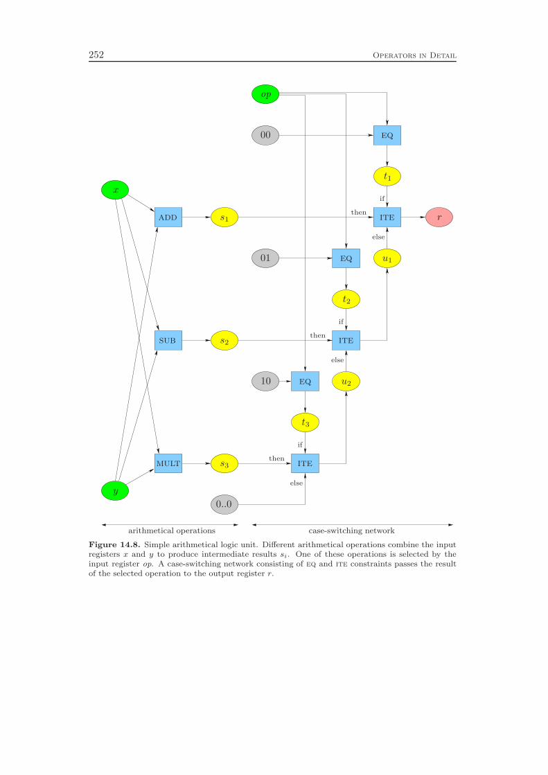
252 Operators in Detail
x
y
op
s1
s2
s3
t1
t2
t3
u1
u2
radd
sub
mult
eq
eq
eq
ite
ite
ite
if
if
if
then
then
then
else
else
else
00
01
10
0..0
arithmetical operations case-switching network
Figure 14.8. Simple arithmetical logic unit. Different arithmetical operations combine the inputregisters x and y to produce intermediate results si. One of these operations is selected by theinput register op. A case-switching network consisting of eq and ite constraints passes the resultof the selected operation to the output register r.
14.15. If-Then-Else 253
In the case x = 1, inequalities (14.51) and (14.52) imply rw = yw, and inequal-ities (14.53) and (14.54) are redundant. Conversely, in the case x = 0, inequal-ities (14.53) and (14.54) force rw = zw and inequalities (14.51) and (14.52) areredundant.
Lemma 14.31. The convex hull Pite = conv{(r, x, y, z) | x ∈ {0, 1}, r, y, z ∈ Z, ly ≤y ≤ uy, lz ≤ z ≤ uz , r = ite(x, y, z)} of the feasible solutions for an ite constraintis full-dimensional if ly < uy, lz < uz , ly < uz , and lz < uy.
Proof. The feasible solutions
(r, x, y, z) ∈{(lz, 0, ly , lz), (lz, 0, uy , lz), (uz, 0, ly , uz), (ly, 1, ly , lz), (uy, 1, uy , lz)
}
define five affinely independent vectors in R4. Thus, the dimension of Pite isdim(Pite) = 4.
Proposition 14.32. Inequalities (14.51) to (14.54) define facets of Pite if ly < uy,lz < uz , ly < uz , and lz < uy.
Proof. Pite is full-dimensional as shown in Lemma 14.31. Thus, it suffices for eachinequality to provide four affinely independent solution vectors that fulfill the in-equality with equality. For inequality (14.51), the solutions
(r, x, y, z) ∈{(ly, 1, ly , lz), (ly, 1, ly , uz), (uy, 1, uy , lz), (uz, 0, ly , uz)
}
meet this criterion. The affinely independent solution vectors
(r, x, y, z) ∈{(ly, 1, ly , lz), (ly, 1, ly , uz), (uy, 1, uy , lz), (lz, 0, uy , lz)
}
fulfill inequality (14.52) with equality. Corresponding solution vectors for inequali-ties (14.53) and (14.54) can be constructed analogously.
14.15.2 Domain Propagation
The domain propagation for if-then-else constraint is depicted in Algorithm 14.25.Step 1 compares the bits of the resultant and the operands y and z. If yb = zb,
we can deduce rb = yb independently from the value of x in Step 1a. If the selectorbit is fixed to x = 1, Step 1b propagates rb = yb. In the other case of x = 0, wecan propagate the equation rb = zb in Step 1c. Steps 1d and 1e apply the inversereasoning of Steps 1b and 1c: if for a bit b we find rb 6= yb, we can conclude x = 0,and if rb 6= zb, we can deduce x = 1.
Step 2 applies exactly the same rules as Step 1 on word level. Independent fromx, the bounds of rw can be tightened in Step 2a. If x is fixed, we can propagaterw = yw or rw = zw in Steps 1b and 1c, respectively. If the bounds of the wordsmake a certain selector value impossible, the selector bit x is fixed to the oppositevalue in Steps 2d and 2e.
14.15.3 Presolving
Presolving for if-then-else constraints applies the same rules as domain propagation,but can also find aggregations of variables. Additionally, we exploit our knowledgeabout equality or inequality of registers. Like for other constraints, we comparepairs of ite constraints to detect further simplifications.
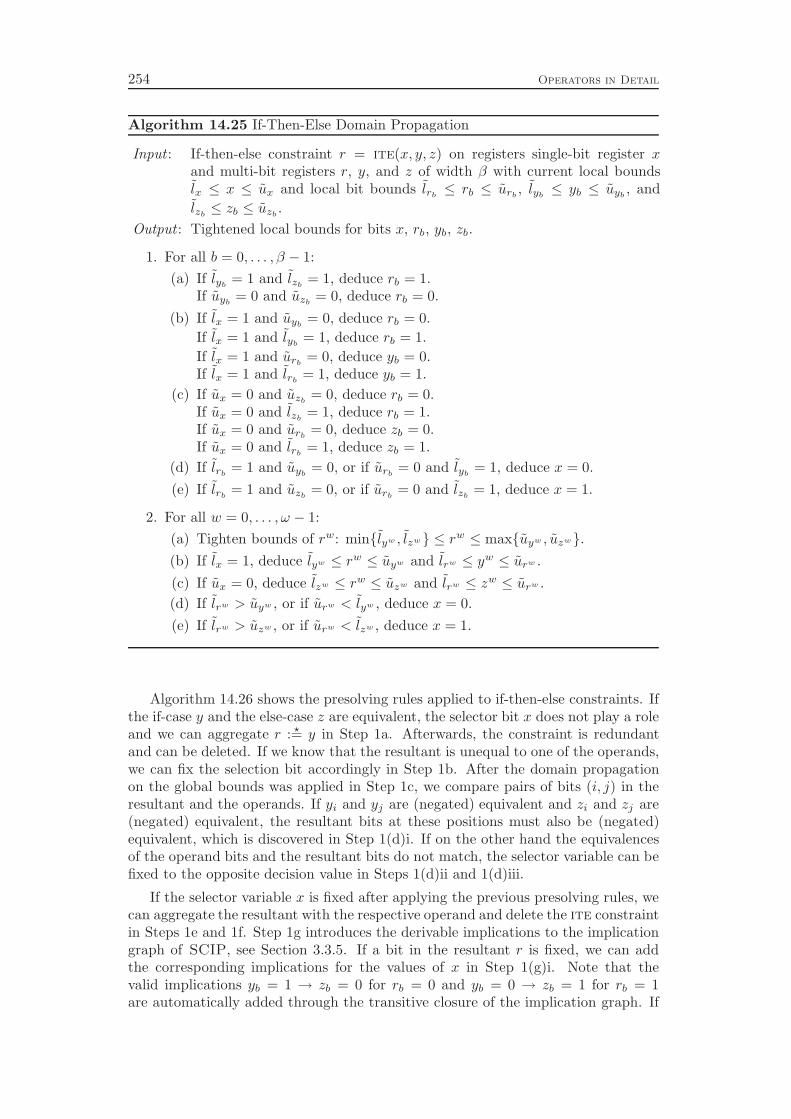
254 Operators in Detail
Algorithm 14.25 If-Then-Else Domain Propagation
Input : If-then-else constraint r = ite(x, y, z) on registers single-bit register xand multi-bit registers r, y, and z of width β with current local boundslx ≤ x ≤ ux and local bit bounds lrb
≤ rb ≤ urb, lyb
≤ yb ≤ uyb, and
lzb≤ zb ≤ uzb
.
Output : Tightened local bounds for bits x, rb, yb, zb.
1. For all b = 0, . . . , β − 1:
(a) If lyb= 1 and lzb
= 1, deduce rb = 1.If uyb
= 0 and uzb= 0, deduce rb = 0.
(b) If lx = 1 and uyb= 0, deduce rb = 0.
If lx = 1 and lyb= 1, deduce rb = 1.
If lx = 1 and urb= 0, deduce yb = 0.
If lx = 1 and lrb= 1, deduce yb = 1.
(c) If ux = 0 and uzb= 0, deduce rb = 0.
If ux = 0 and lzb= 1, deduce rb = 1.
If ux = 0 and urb= 0, deduce zb = 0.
If ux = 0 and lrb= 1, deduce zb = 1.
(d) If lrb= 1 and uyb
= 0, or if urb= 0 and lyb
= 1, deduce x = 0.
(e) If lrb= 1 and uzb
= 0, or if urb= 0 and lzb
= 1, deduce x = 1.
2. For all w = 0, . . . , ω − 1:
(a) Tighten bounds of rw: min{lyw , lzw} ≤ rw ≤ max{uyw , uzw}.
(b) If lx = 1, deduce lyw ≤ rw ≤ uyw and lrw ≤ yw ≤ urw .
(c) If ux = 0, deduce lzw ≤ rw ≤ uzw and lrw ≤ zw ≤ urw .
(d) If lrw > uyw , or if urw < lyw , deduce x = 0.
(e) If lrw > uzw , or if urw < lzw , deduce x = 1.
Algorithm 14.26 shows the presolving rules applied to if-then-else constraints. Ifthe if-case y and the else-case z are equivalent, the selector bit x does not play a roleand we can aggregate r : ⋆= y in Step 1a. Afterwards, the constraint is redundantand can be deleted. If we know that the resultant is unequal to one of the operands,we can fix the selection bit accordingly in Step 1b. After the domain propagationon the global bounds was applied in Step 1c, we compare pairs of bits (i, j) in theresultant and the operands. If yi and yj are (negated) equivalent and zi and zj are(negated) equivalent, the resultant bits at these positions must also be (negated)equivalent, which is discovered in Step 1(d)i. If on the other hand the equivalencesof the operand bits and the resultant bits do not match, the selector variable can befixed to the opposite decision value in Steps 1(d)ii and 1(d)iii.
If the selector variable x is fixed after applying the previous presolving rules, wecan aggregate the resultant with the respective operand and delete the ite constraintin Steps 1e and 1f. Step 1g introduces the derivable implications to the implicationgraph of SCIP, see Section 3.3.5. If a bit in the resultant r is fixed, we can addthe corresponding implications for the values of x in Step 1(g)i. Note that thevalid implications yb = 1 → zb = 0 for rb = 0 and yb = 0 → zb = 1 for rb = 1are automatically added through the transitive closure of the implication graph. If

14.15. If-Then-Else 255
Algorithm 14.26 If-Then-Else Presolving
1. For all active if-then-else constraints r = ite(x, y, z):
(a) If y ⋆= z, aggregate r : ⋆= y and delete the constraint.
(b) If r Y⋆= z, fix x := 1.
If r Y⋆= y, fix x := 0.
(c) Apply domain propagation Algorithm 14.25 on the global bounds.
(d) For all i, j ∈ {0, . . . , β − 1} with i < j:i. If yi
⋆= yj and zi⋆= zj , aggregate ri : ⋆= rj .
If yi Y⋆= yj and zi Y
⋆= zj , aggregate ri : ⋆= 1− rj .
ii. If yi⋆= yj and ri Y
⋆= rj , fix x := 0.
If yi Y⋆= yj and ri
⋆= rj , fix x := 0.
iii. If zi⋆= zj and ri Y
⋆= rj , fix x := 1.
If zi Y⋆= zj and ri
⋆= rj , fix x := 1.
(e) If x = 1, aggregate r : ⋆= y and delete the constraint.
(f) If x = 0, aggregate r : ⋆= z and delete the constraint.
(g) For all b = 0, . . . , β − 1, add the following implications to the implicationgraph of SCIP:
i. If rb = 0, add implications x = 1→ yb = 0 and x = 0→ zb = 0.If rb = 1, add implications x = 1→ yb = 1 and x = 0→ zb = 1.
ii. If yb = 0, add implications x = 1→ rb = 0 and zb = 0→ rb = 0.If yb = 1, add implications x = 1→ rb = 1 and zb = 1→ rb = 1.
iii. If zb = 0, add implications x = 0→ rb = 0 and yb = 0→ rb = 0.If zb = 1, add implications x = 0→ rb = 1 and yb = 1→ rb = 1.
2. For all pairs of active if-then-else constraints r = ite(x, y, z) and r′ =eq(x′, y′, z′) with βr ≥ βr′ :
(a) For all b = 0, . . . , βr − 1:i. If x ⋆= x′, yb
⋆= y′b, and zb⋆= z′b, aggregate rb : ⋆= r′b.
If x ⋆= x′, yb Y⋆= y′b, and zb Y
⋆= z′b, aggregate rb : ⋆= 1− r′b.
ii. If x Y⋆= x′, yb
⋆= z′b, and zb⋆= y′b, aggregate rb : ⋆= r′b.
If x Y⋆= x′, yb Y
⋆= z′b, and zb Y
⋆= y′b, aggregate rb : ⋆= 1− r′b.
If all of the resultant bits were aggregated, delete r′ = eq(x′, y′, z′).
(b) If βr = βr′ and r Y⋆= r′, add the following implications to the implication
graph of SCIP:i. If y ⋆= y′, add x = 1→ x′ = 0.
ii. If z ⋆= z′, add x = 0→ x′ = 1.iii. If y ⋆= z′, add x = 1→ x′ = 1.iv. If z ⋆= y′, add x = 0→ x′ = 0.
(c) If y ⋆= r′ and x = 1→ x′ = 1 holds, replace y by y′.If y ⋆= r′ and x = 1→ x′ = 0 holds, replace y by z′.
(d) If z ⋆= r′ and x = 0→ x′ = 1 holds, replace z by y′.If z ⋆= r′ and x = 0→ x′ = 0 holds, replace z by z′.
(e) If y′ ⋆= r and x′ = 1→ x = 1 holds, replace y′ by y.If y′ ⋆= r and x′ = 1→ x = 0 holds, replace y′ by z.
(f) If z′ ⋆= r and x′ = 0→ x = 1 holds, replace z′ by y.If z′ ⋆= r and x′ = 0→ x = 0 holds, replace z′ by z.
256 Operators in Detail
one of the operand bits is fixed, similar implications can be added in Steps 1(g)iiand 1(g)iii.
In the pairwise presolving Step 2 we can also look at the individual bits of thetwo constraints in Step 2a. As usual, we define r′b = y′b = z′b = 0 if b ≥ βr′ .Now if the two selector variables x and x′ are equivalent, the bits of the if-cases yb
and y′b are equivalent, and the bits of the else-cases zb and z′b are also equivalent,the resultant bits rb and r′b must also be equivalent. If the operand bits arepairwise negated equivalent, the resultant bits must also be negated equivalent.Conversely, if the selector variables are negated equivalent and the operand bitsare (negated) equivalent with interchanged roles, the resultant bits must also be(negated) equivalent.
If we know that the resultants have the same width but are unequal, the implica-tions of Step 2b can be deduced: if an operand from the first constraint is equivalentto an operand of the second constraint, the selector bits x and x′ cannot both selectthis operand, since otherwise, the resultants would also be equivalent. Note that theimplications of Steps 2(b)i and 2(b)ii immediately fix the selector bits if x ⋆= x′, and
Steps 2(b)iii and 2(b)iv fix them if x Y⋆= x′. Due to Steps 1e and 1f, this would also
lead to the aggregation of the resultants and the deletion of the two constraints.Steps 2c to 2f check for chainings of ite constraints. If the resultant r′ of one con-
straint r′ = ite(x′, y′, z′) appears as operand in another constraint r = ite(x, y, z),and if there is a matching implication between the selection variables x and x′, wecan substitute the resultant r′ by the corresponding operand y′ or z′ in the sec-ond constraint. Thereby, we avoid the unnecessary detour via r′ and the first iteconstraint. For example, if there are two constraints
r = ite(x, r′, z) and r′ = ite(x, y′, z′),
we can replace r′ by y′ in the first constraint which gives
r = ite(x, y′, z) and r′ = ite(x, y′, z′).
This substitution simplifies the structure of the function graph, see Section 13.2,and offers additional potential for the irrelevance detection of Section 15.2. Forexample, suppose r′ is not used in other constraints. Then we can delete the secondconstraint from the problem because it is not relevant for the validity of the property.If after the deletion of the constraint z′ does only appear as the resultant of a singleconstraint, it can also be deleted from the problem instance for the same reason.This can trigger a chain of problem reductions with the possibility to delete a wholesubtree from the function graph.
14.16 Zero Extension
With the zero extension operator
zeroext : [µ]→ [β], x 7→ r = zeroext(x)
a register x is copied into a (usually wider) register r with the excessive bits of rfixed to zero. Although usually β > µ we define the constraint for general registerwidths:
r = zeroext(x) ⇔ ∀b ∈ {0, . . . , β − 1} : rb =
{
xb if b < µ,
0 if b ≥ µ.
14.17. Sign Extension 257
Thereby it is possible with β < µ to extract a low-significant subword of a register.Nevertheless, the zero extension operator can easily be implemented by performingthe corresponding aggregations rb : ⋆= xb for b < µ and fixings rb := 0 for b ≥ µ inthe presolving stage of SCIP. Afterwards, the constraint can be deleted from theproblem formulation.
14.17 Sign Extension
Like the zero extension, the sign extension operator
signext : [µ]→ [β], x 7→ r = signext(x)
copies a register x into a register r. But in this case, the excessive bits of r are allequal to the most significant bit of x, thereby preserving the signed value in the two’scomplement representation. The constraint is defined for general register widths µand β as
r = signext(x) ⇔ ∀b ∈ {0, . . . , β − 1} : rb =
{
xb if b < µ,
xµ−1 if b ≥ µ.
Again, we can implement the operator by performing the corresponding aggregationsrb : ⋆= xb for b < µ and rb : ⋆= xµ−1 for b ≥ µ in the presolving stage of SCIP anddeleting the constraint afterwards.
14.18 Concatenation
Concatenation with the operator
concat : [β]× [µ]→ [β + µ], (x, y) 7→ r = concat(x, y)
means to form a single register bit string out of the two input registers by chaining uptheir individual bits. The bits of the first input register x form the high-significantpart of the result, while the bits of the second input register y are used in thelow-significant part:
r = concat(x, y) ⇔ ∀b ∈ {0, . . . , β + µ− 1} : rb =
{
yb if b < µ,
xb−µ if b ≥ µ.
Like the other word extension operators, concatenation can be implemented byperforming the necessary presolving aggregations rb : ⋆= yb for b < µ and rb : ⋆= xb−µ
for b ≥ µ and deleting the constraint afterwards.
14.19 Shift Left
The shift left operation
shl : [β]× [µ]→ [β], (x, y) 7→ r = shl(x, y)
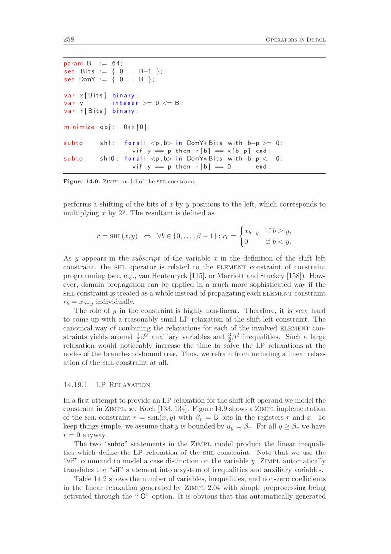
258 Operators in Detail
param B := 64 ;s e t B i t s := { 0 . . B−1 } ;s e t DomY := { 0 . . B } ;
va r x [ B i t s ] b i n a r y ;va r y i n t e g e r >= 0 <= B;va r r [ B i t s ] b i n a r y ;
min imize ob j : 0∗ x [ 0 ] ;
subto s h l : f o r a l l <p , b> i n DomY∗ B i t s w i th b−p >= 0 :v i f y == p then r [ b ] == x [ b−p ] end ;
subto s h l 0 : f o r a l l <p , b> i n DomY∗ B i t s w i th b−p < 0 :v i f y == p then r [ b ] == 0 end ;
Figure 14.9. Zimpl model of the shl constraint.
performs a shifting of the bits of x by y positions to the left, which corresponds tomultiplying x by 2y. The resultant is defined as
r = shl(x, y) ⇔ ∀b ∈ {0, . . . , β − 1} : rb =
{
xb−y if b ≥ y,
0 if b < y.
As y appears in the subscript of the variable x in the definition of the shift leftconstraint, the shl operator is related to the element constraint of constraintprogramming (see, e.g., van Hentenryck [115], or Marriott and Stuckey [158]). How-ever, domain propagation can be applied in a much more sophisticated way if theshl constraint is treated as a whole instead of propagating each element constraintrb = xb−y individually.
The role of y in the constraint is highly non-linear. Therefore, it is very hardto come up with a reasonably small LP relaxation of the shift left constraint. Thecanonical way of combining the relaxations for each of the involved element con-straints yields around 1
2β2 auxiliary variables and 3
2β2 inequalities. Such a large
relaxation would noticeably increase the time to solve the LP relaxations at thenodes of the branch-and-bound tree. Thus, we refrain from including a linear relax-ation of the shl constraint at all.
14.19.1 LP Relaxation
In a first attempt to provide an LP relaxation for the shift left operand we model theconstraint in Zimpl, see Koch [133, 134]. Figure 14.9 shows a Zimpl implementationof the shl constraint r = shl(x, y) with βr = B bits in the registers r and x. Tokeep things simple, we assume that y is bounded by uy = βr. For all y ≥ βr we haver = 0 anyway.
The two “subto” statements in the Zimpl model produce the linear inequali-ties which define the LP relaxation of the shl constraint. Note that we use the“vif” command to model a case distinction on the variable y. Zimpl automaticallytranslates the “vif” statement into a system of inequalities and auxiliary variables.
Table 14.2 shows the number of variables, inequalities, and non-zero coefficientsin the linear relaxation generated by Zimpl 2.04 with simple preprocessing beingactivated through the “-O” option. It is obvious that this automatically generated
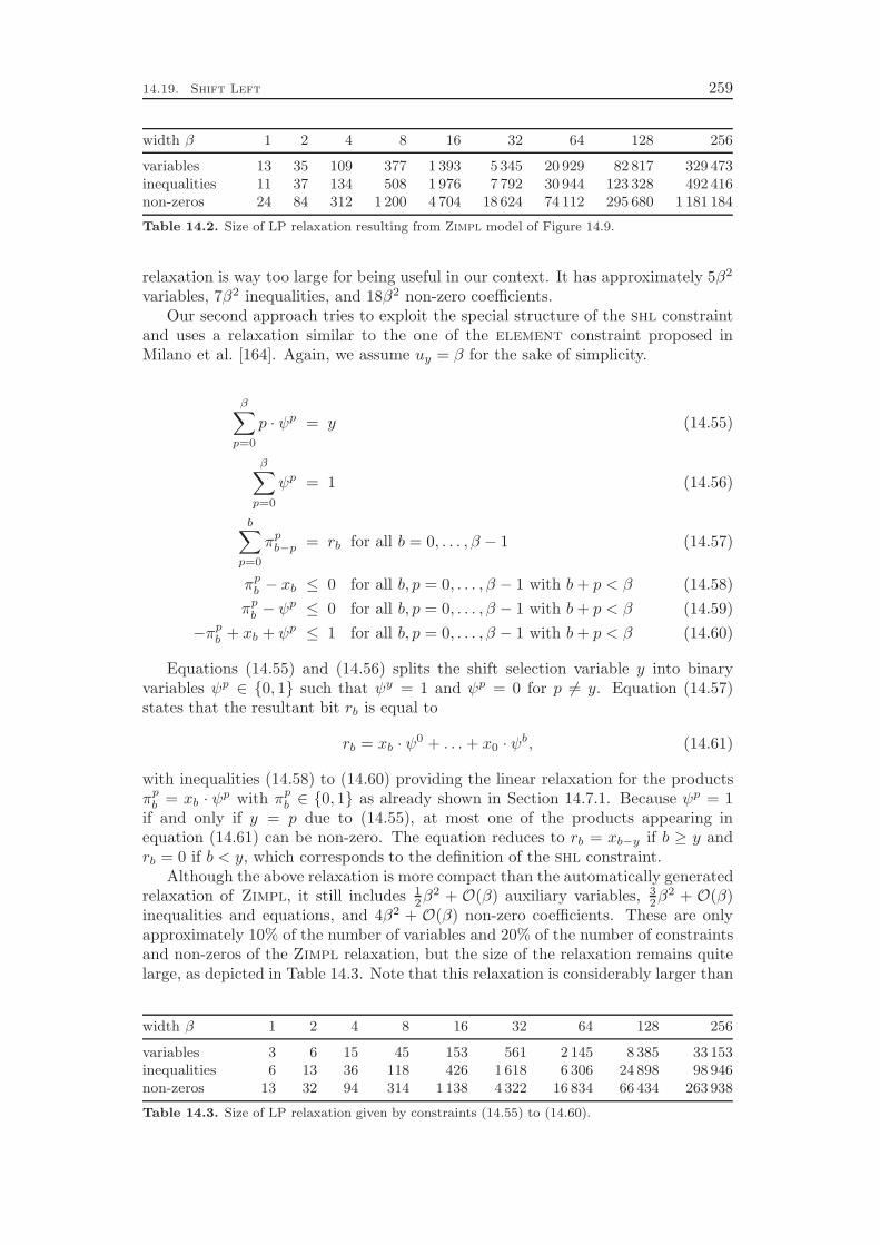
14.19. Shift Left 259
width β 1 2 4 8 16 32 64 128 256
variables 13 35 109 377 1 393 5 345 20 929 82 817 329 473inequalities 11 37 134 508 1 976 7 792 30 944 123 328 492 416non-zeros 24 84 312 1 200 4 704 18 624 74 112 295 680 1 181 184
Table 14.2. Size of LP relaxation resulting from Zimpl model of Figure 14.9.
relaxation is way too large for being useful in our context. It has approximately 5β2
variables, 7β2 inequalities, and 18β2 non-zero coefficients.Our second approach tries to exploit the special structure of the shl constraint
and uses a relaxation similar to the one of the element constraint proposed inMilano et al. [164]. Again, we assume uy = β for the sake of simplicity.
β∑
p=0
p · ψp = y (14.55)
β∑
p=0
ψp = 1 (14.56)
b∑
p=0
πpb−p = rb for all b = 0, . . . , β − 1 (14.57)
πpb − xb ≤ 0 for all b, p = 0, . . . , β − 1 with b+ p < β (14.58)
πpb − ψ
p ≤ 0 for all b, p = 0, . . . , β − 1 with b+ p < β (14.59)
−πpb + xb + ψp ≤ 1 for all b, p = 0, . . . , β − 1 with b+ p < β (14.60)
Equations (14.55) and (14.56) splits the shift selection variable y into binaryvariables ψp ∈ {0, 1} such that ψy = 1 and ψp = 0 for p 6= y. Equation (14.57)states that the resultant bit rb is equal to
rb = xb · ψ0 + . . . + x0 · ψ
b, (14.61)
with inequalities (14.58) to (14.60) providing the linear relaxation for the productsπp
b = xb · ψp with πp
b ∈ {0, 1} as already shown in Section 14.7.1. Because ψp = 1if and only if y = p due to (14.55), at most one of the products appearing inequation (14.61) can be non-zero. The equation reduces to rb = xb−y if b ≥ y andrb = 0 if b < y, which corresponds to the definition of the shl constraint.
Although the above relaxation is more compact than the automatically generatedrelaxation of Zimpl, it still includes 1
2β2 + O(β) auxiliary variables, 3
2β2 + O(β)
inequalities and equations, and 4β2 + O(β) non-zero coefficients. These are onlyapproximately 10% of the number of variables and 20% of the number of constraintsand non-zeros of the Zimpl relaxation, but the size of the relaxation remains quitelarge, as depicted in Table 14.3. Note that this relaxation is considerably larger than
width β 1 2 4 8 16 32 64 128 256
variables 3 6 15 45 153 561 2 145 8 385 33 153inequalities 6 13 36 118 426 1 618 6 306 24 898 98 946non-zeros 13 32 94 314 1 138 4 322 16 834 66 434 263 938
Table 14.3. Size of LP relaxation given by constraints (14.55) to (14.60).
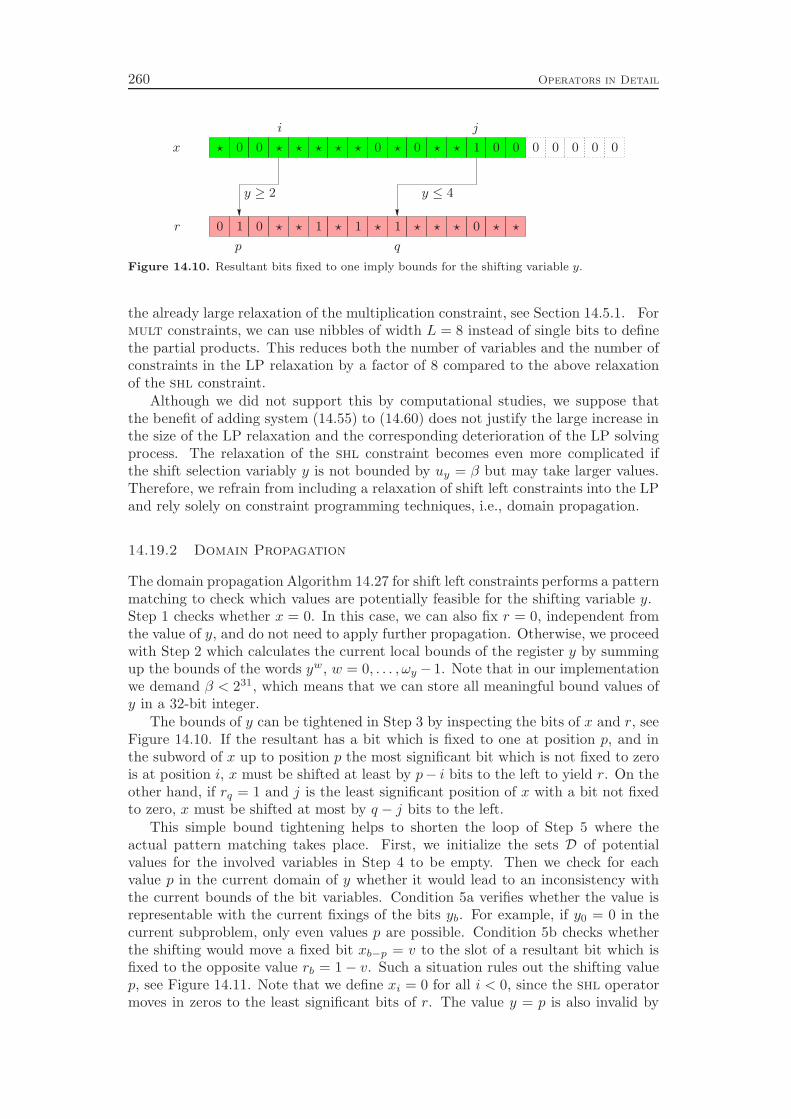
260 Operators in Detail
000
000000 00000
1111
1
⋆⋆⋆⋆⋆⋆⋆⋆⋆
⋆⋆⋆⋆⋆⋆⋆⋆⋆x
r
i j
p q
y ≥ 2 y ≤ 4
Figure 14.10. Resultant bits fixed to one imply bounds for the shifting variable y.
the already large relaxation of the multiplication constraint, see Section 14.5.1. Formult constraints, we can use nibbles of width L = 8 instead of single bits to definethe partial products. This reduces both the number of variables and the number ofconstraints in the LP relaxation by a factor of 8 compared to the above relaxationof the shl constraint.
Although we did not support this by computational studies, we suppose thatthe benefit of adding system (14.55) to (14.60) does not justify the large increase inthe size of the LP relaxation and the corresponding deterioration of the LP solvingprocess. The relaxation of the shl constraint becomes even more complicated ifthe shift selection variably y is not bounded by uy = β but may take larger values.Therefore, we refrain from including a relaxation of shift left constraints into the LPand rely solely on constraint programming techniques, i.e., domain propagation.
14.19.2 Domain Propagation
The domain propagation Algorithm 14.27 for shift left constraints performs a patternmatching to check which values are potentially feasible for the shifting variable y.Step 1 checks whether x = 0. In this case, we can also fix r = 0, independent fromthe value of y, and do not need to apply further propagation. Otherwise, we proceedwith Step 2 which calculates the current local bounds of the register y by summingup the bounds of the words yw, w = 0, . . . , ωy − 1. Note that in our implementationwe demand β < 231, which means that we can store all meaningful bound values ofy in a 32-bit integer.
The bounds of y can be tightened in Step 3 by inspecting the bits of x and r, seeFigure 14.10. If the resultant has a bit which is fixed to one at position p, and inthe subword of x up to position p the most significant bit which is not fixed to zerois at position i, x must be shifted at least by p− i bits to the left to yield r. On theother hand, if rq = 1 and j is the least significant position of x with a bit not fixedto zero, x must be shifted at most by q − j bits to the left.
This simple bound tightening helps to shorten the loop of Step 5 where theactual pattern matching takes place. First, we initialize the sets D of potentialvalues for the involved variables in Step 4 to be empty. Then we check for eachvalue p in the current domain of y whether it would lead to an inconsistency withthe current bounds of the bit variables. Condition 5a verifies whether the value isrepresentable with the current fixings of the bits yb. For example, if y0 = 0 in thecurrent subproblem, only even values p are possible. Condition 5b checks whetherthe shifting would move a fixed bit xb−p = v to the slot of a resultant bit which isfixed to the opposite value rb = 1− v. Such a situation rules out the shifting valuep, see Figure 14.11. Note that we define xi = 0 for all i < 0, since the shl operatormoves in zeros to the least significant bits of r. The value y = p is also invalid by

14.19. Shift Left 261
Algorithm 14.27 Shift Left Domain Propagation
Input : Shift left constraint r = shl(x, y) on registers r and x of width βr = βx = βwith current local bit bounds lrb
≤ rb ≤ urband lxb
≤ xb ≤ uxb, and y
of width βy = µ with current local bit bounds lyb≤ yb ≤ uyb
and word
bounds lyw ≤ yw ≤ uyw .
Output : Tightened local bounds for bits rb, xb, and yb, and words yw.
1. If uxb= 0 for all b = 0, . . . , β−1, deduce rb = 0 for all b and abort propagation.
2. Calculate bounds for the register y from the words’ bounds:
ly :=
ωy−1∑
w=0
2wW lyw and uy :=
ωy−1∑
w=0
2wW uyw .
3. Let br=1min := min{b | lrb
= 1} and br=1max := max{b | lrb
= 1}.
Let bx6=0min := min{b | uxb
= 1} and bx6=0max := max{b | uxb
= 1 and b ≤ br=1max}.
Tighten ly := max{ly, b
r=1max − b
x6=0max
}and uy := min
{uy , b
r=1min − b
x6=0min
}.
4. Initialize Dxb:= ∅ and Drb
:= ∅ for all b = 0, . . . , β − 1, Dyb:= ∅ for all
b = 0, . . . , µ− 1, and Dy := ∅.
5. For all p = ly, . . . , uy :
Let p =∑µ−1
b=0 2bpb be the bit decomposition of p. If the following holds:
(a) pb ∈ {lyb, uyb} for all b = 0, . . . , µ− 1,
(b) Db := {lrb, urb} ∩ {lxb−p
, uxb−p} 6= ∅ for all b = 0, . . . , β − 1, and
(c) there is no bit b ∈ {0, . . . , β − 1} with rb Y⋆= xb−p,
the shifting value y = p is valid. In this case, update
(a) Dy := Dy ∪ {p},
(b) Dyb:= Dyb
∪ {pb} for all b = 0, . . . , µ− 1,
(c) Drb:= Drb
∪ Db for all b = 0, . . . , β − 1,
(d) Dxb:= Dxb
∪ Db+p for all b = 0, . . . , β − 1− p, and
(e) Dxb:= {lxb
, uxb} for all b = β − p, . . . , β − 1.
6. Tighten word bounds of yw, w = 0, . . . , ωy − 1, corresponding to the registerbounds min{Dy} ≤ y ≤ max{Dy}.
7. For all b = 0, . . . , µ− 1: Tighten min{Dyb} ≤ yb ≤ max{Dyb
}.For all b = 0, . . . , β − 1: Tighten min{Drb
} ≤ rb ≤ max{Drb}.
For all b = 0, . . . , β − 1: Tighten min{Dxb} ≤ xb ≤ max{Dxb
}.
0
000000
00
000000 00
000000 0000
0001
1111
1
1
⋆⋆⋆⋆⋆⋆⋆⋆⋆
⋆⋆⋆⋆⋆⋆⋆⋆⋆
⋆⋆⋆⋆⋆⋆⋆⋆⋆
⋆⋆⋆⋆⋆⋆⋆⋆⋆
x
r
y = 2
y = 3
y = 4
Figure 14.11. Pattern matching to identify potential values of y.
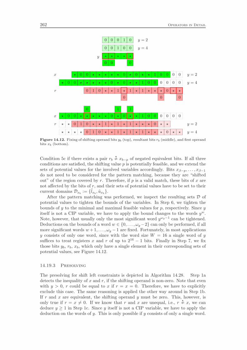
262 Operators in Detail
000000
0 0 0
000
000
0
000
000
000000 0000
000000 00
0000
0000
00001
1 1 1 1
1111
1111
11
1
1
1
1
⋆⋆⋆⋆
⋆⋆ ⋆
⋆
⋆ ⋆⋆⋆⋆⋆
⋆⋆ ⋆ ⋆ ⋆
⋆⋆⋆⋆⋆⋆⋆⋆
⋆ ⋆⋆⋆⋆⋆⋆⋆⋆
⋆⋆⋆⋆⋆
⋆⋆
⋆⋆
⋆⋆
⋆⋆⋆⋆⋆⋆⋆⋆⋆
⋆⋆⋆⋆⋆⋆⋆⋆⋆
y
x
x
r
r
y = 2
y = 2
y = 2
y = 4
y = 4
y = 4
Figure 14.12. Fixing of shifting operand bits yb (top), resultant bits rb (middle), and first operandbits xb (bottom).
Condition 5c if there exists a pair rb Y⋆= xb−p of negated equivalent bits. If all three
conditions are satisfied, the shifting value p is potentially feasible, and we extend thesets of potential values for the involved variables accordingly. Bits xβ−p, . . . , xβ−1
do not need to be considered for the pattern matching, because they are “shiftedout” of the region covered by r. Therefore, if p is a valid match, these bits of x arenot affected by the bits of r, and their sets of potential values have to be set to theircurrent domains Dxb
:= {lxb, uxb}.
After the pattern matching was performed, we inspect the resulting sets D ofpotential values to tighten the bounds of the variables. In Step 6, we tighten thebounds of y to the minimal and maximal feasible values for p, respectively. Since yitself is not a CIP variable, we have to apply the bound changes to the words yw.Note, however, that usually only the most significant word yωy−1 can be tightened.Deductions on the bounds of a word w ∈ {0, . . . , ωy−2} can only be performed, if allmore significant words w+1, . . . , ωy − 1 are fixed. Fortunately, in most applicationsy consists of only one word, since with the word size W = 16 a single word of ysuffices to treat registers x and r of up to 216 − 1 bits. Finally in Step 7, we fixthose bits yb, rb, xb, which only have a single element in their corresponding sets ofpotential values, see Figure 14.12.
14.19.3 Presolving
The presolving for shift left constraints is depicted in Algorithm 14.28. Step 1adetects the inequality of x and r, if the shifting operand is non-zero. Note that evenwith y > 0, r could be equal to x if r = x = 0. Therefore, we have to explicitlyexclude this case. The same reasoning is applied the other way around in Step 1b.If r and x are equivalent, the shifting operand y must be zero. This, however, isonly true if r = x 6= 0. If we know that r and x are unequal, i.e., r Y
⋆= x, we can
deduce y ≥ 1 in Step 1c. Since y itself is not a CIP variable, we have to apply thededuction on the words of y. This is only possible if y consists of only a single word.
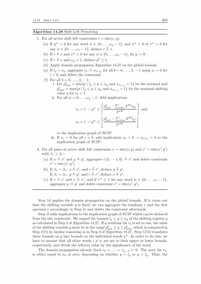
14.19. Shift Left 263
Algorithm 14.28 Shift Left Presolving
1. For all active shift left constraints r = shl(x, y):
(a) If yw > 0 for any word w ∈ {0, . . . , ωy − 1}, and xw > 0 or rw > 0 for
any w ∈ {0, . . . , ωx − 1}, deduce r Y⋆= x.
(b) If r ⋆= x and xw > 0 for any w ∈ {0, . . . , ωx − 1}, fix y := 0.
(c) If r Y⋆= x and ωy = 1, deduce y0 ≥ 1.
(d) Apply domain propagation Algorithm 14.27 on the global bounds.
(e) If ly = uy, aggregate rb : ⋆= xb−ly for all b = 0, . . . , βr − 1 using xi = 0 fori < 0, and delete the constraint.
(f) For all b = 0, . . . , βr − 1:i. Let pb
min = min{p | ly ≤ p ≤ uy and uxb−p= 1} be the minimal and
pbmax = max{p | ly ≤ p ≤ uy and uxb−p
= 1} be the maximal shiftingvalue y for rb = 1.
ii. For all w = 0, . . . , ωy − 1: Add implications
rb = 1→ yw ≥
⌈
pbmin −
∑
i 6=w 2iWuyi
2wW
⌉
and
rb = 1→ yw ≤
⌊
pbmax −
∑
i 6=w 2iW lyi
2wW
⌋
to the implication graph of SCIP.iii. If xi = 0 for all i < b, add implication xb = 0 → rb+ly = 0 to the
implication graph of SCIP.
2. For all pairs of active shift left constraints r = shl(x, y) and r′ = shl(x′, y′)with βr ≥ βr′ :
(a) If x ⋆= x′ and y ⋆= y′, aggregate r[βr′ − 1, 0] : ⋆= r′ and delete constraintr′ = shl(x′, y′).
(b) If βr = βr′ , x ⋆= x′, and r Y⋆= r′, deduce y Y
⋆= y′.
If βr = βr′ , y ⋆= y′, and r Y⋆= r′, deduce x Y
⋆= x′.
(c) If r ⋆= r′ and x ⋆= x′, and if rw ≥ 1 for any word w ∈ {0, . . . , ωr − 1},aggregate y : ⋆= y′ and delete constraint r′ = shl(x′, y′).
Step 1d applies the domain propagation on the global bounds. If it turns outthat the shifting variable y is fixed, we can aggregate the resultant r and the firstoperand x accordingly in Step 1e and delete the constraint afterwards.
Step 1f adds implications to the implication graph of SCIP which can be deducedfrom the shl constraint. We regard the bounds ly ≤ y ≤ uy of the shifting register yas calculated in Step 2 of Algorithm 14.27. If a resultant bit rb is set to one, the valueof the shifting variable y must be in the range pb
min ≤ y ≤ pbmax, which is computed in
Step 1(f)i by similar reasoning as in Step 3 of Algorithm 14.27. Step 1(f)ii translatesthese bounds on y into bounds on the individual words yw. In order to do this, wehave to assume that all other words i 6= w are set to their upper or lower bounds,respectively, and divide the leftover value by the significance of the word.
The domain propagation already fixed r0 = . . . = rly−1 = 0. The next bit rlyis either equal to x0 or zero, depending on whether y = ly or y > ly. Thus, the
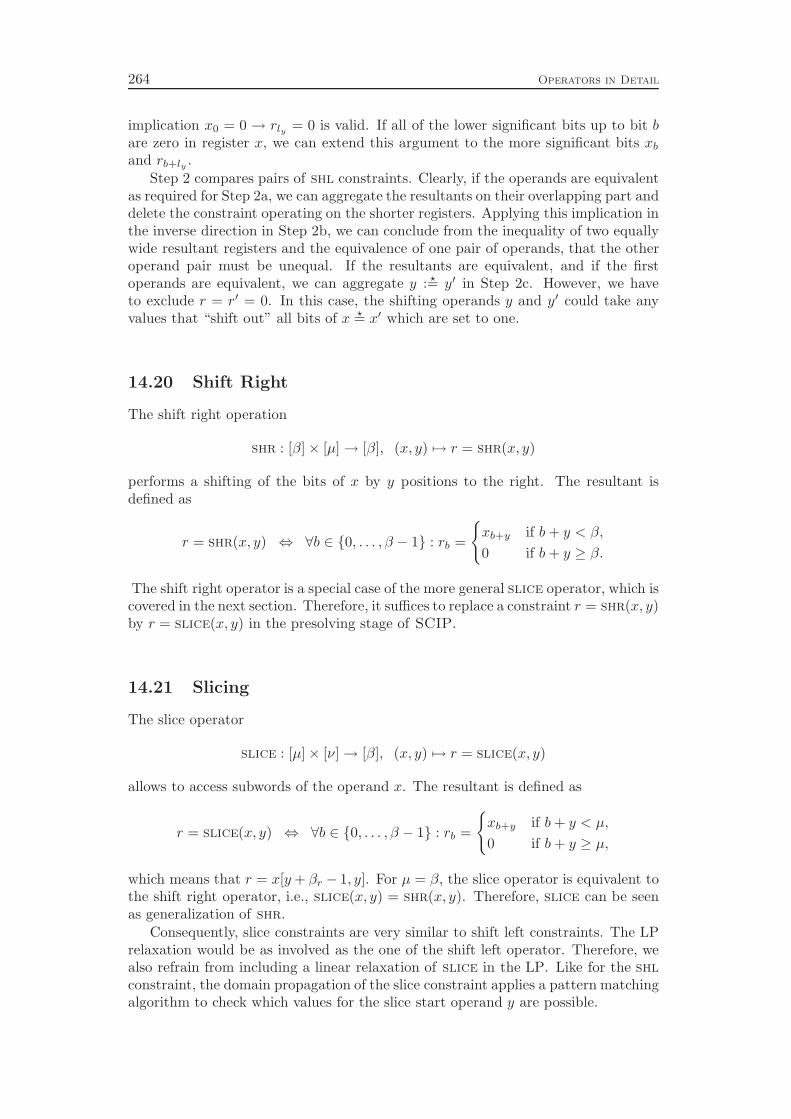
264 Operators in Detail
implication x0 = 0 → rly = 0 is valid. If all of the lower significant bits up to bit bare zero in register x, we can extend this argument to the more significant bits xb
and rb+ly .Step 2 compares pairs of shl constraints. Clearly, if the operands are equivalent
as required for Step 2a, we can aggregate the resultants on their overlapping part anddelete the constraint operating on the shorter registers. Applying this implication inthe inverse direction in Step 2b, we can conclude from the inequality of two equallywide resultant registers and the equivalence of one pair of operands, that the otheroperand pair must be unequal. If the resultants are equivalent, and if the firstoperands are equivalent, we can aggregate y : ⋆= y′ in Step 2c. However, we haveto exclude r = r′ = 0. In this case, the shifting operands y and y′ could take anyvalues that “shift out” all bits of x ⋆= x′ which are set to one.
14.20 Shift Right
The shift right operation
shr : [β]× [µ]→ [β], (x, y) 7→ r = shr(x, y)
performs a shifting of the bits of x by y positions to the right. The resultant isdefined as
r = shr(x, y) ⇔ ∀b ∈ {0, . . . , β − 1} : rb =
{
xb+y if b+ y < β,
0 if b+ y ≥ β.
The shift right operator is a special case of the more general slice operator, which iscovered in the next section. Therefore, it suffices to replace a constraint r = shr(x, y)by r = slice(x, y) in the presolving stage of SCIP.
14.21 Slicing
The slice operator
slice : [µ]× [ν]→ [β], (x, y) 7→ r = slice(x, y)
allows to access subwords of the operand x. The resultant is defined as
r = slice(x, y) ⇔ ∀b ∈ {0, . . . , β − 1} : rb =
{
xb+y if b+ y < µ,
0 if b+ y ≥ µ,
which means that r = x[y+ βr − 1, y]. For µ = β, the slice operator is equivalent tothe shift right operator, i.e., slice(x, y) = shr(x, y). Therefore, slice can be seenas generalization of shr.
Consequently, slice constraints are very similar to shift left constraints. The LPrelaxation would be as involved as the one of the shift left operator. Therefore, wealso refrain from including a linear relaxation of slice in the LP. Like for the shlconstraint, the domain propagation of the slice constraint applies a pattern matchingalgorithm to check which values for the slice start operand y are possible.
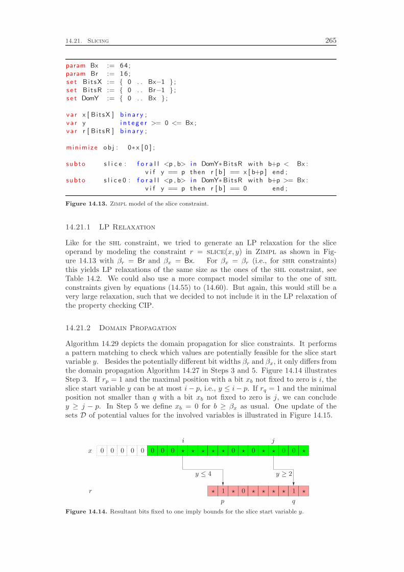
14.21. Slicing 265
param Bx := 64 ;param Br := 16 ;s e t Bi t sX := { 0 . . Bx−1 } ;s e t Bi t sR := { 0 . . Br−1 } ;s e t DomY := { 0 . . Bx } ;
va r x [ B i t sX ] b i n a r y ;va r y i n t e g e r >= 0 <= Bx ;va r r [ B i t sR ] b i n a r y ;
min imize ob j : 0∗ x [ 0 ] ;
subto s l i c e : f o r a l l <p , b> i n DomY∗Bit sR with b+p < Bx :v i f y == p then r [ b ] == x [ b+p ] end ;
subto s l i c e 0 : f o r a l l <p , b> i n DomY∗Bit sR with b+p >= Bx :v i f y == p then r [ b ] == 0 end ;
Figure 14.13. Zimpl model of the slice constraint.
14.21.1 LP Relaxation
Like for the shl constraint, we tried to generate an LP relaxation for the sliceoperand by modeling the constraint r = slice(x, y) in Zimpl as shown in Fig-ure 14.13 with βr = Br and βx = Bx. For βx = βr (i.e., for shr constraints)this yields LP relaxations of the same size as the ones of the shl constraint, seeTable 14.2. We could also use a more compact model similar to the one of shlconstraints given by equations (14.55) to (14.60). But again, this would still be avery large relaxation, such that we decided to not include it in the LP relaxation ofthe property checking CIP.
14.21.2 Domain Propagation
Algorithm 14.29 depicts the domain propagation for slice constraints. It performsa pattern matching to check which values are potentially feasible for the slice startvariable y. Besides the potentially different bit widths βr and βx, it only differs fromthe domain propagation Algorithm 14.27 in Steps 3 and 5. Figure 14.14 illustratesStep 3. If rp = 1 and the maximal position with a bit xb not fixed to zero is i, theslice start variable y can be at most i− p, i.e., y ≤ i− p. If rq = 1 and the minimalposition not smaller than q with a bit xb not fixed to zero is j, we can concludey ≥ j − p. In Step 5 we define xb = 0 for b ≥ βx as usual. One update of thesets D of potential values for the involved variables is illustrated in Figure 14.15.
0000000
0
00000
11
⋆⋆⋆⋆⋆⋆⋆⋆⋆
⋆⋆⋆⋆⋆⋆⋆
x
r
i j
p q
y ≥ 2y ≤ 4
Figure 14.14. Resultant bits fixed to one imply bounds for the slice start variable y.

266 Operators in Detail
Algorithm 14.29 Slice Domain Propagation
Input : Slice constraint r = slice(x, y) on registers r, x, and y with current localbit bounds lrb
≤ rb ≤ urb, lxb
≤ xb ≤ uxb, and lyb
≤ yb ≤ uyb, and current
local word bounds lyw ≤ yw ≤ uyw .
Output : Tightened local bounds for bits rb, xb, and yb, and words yw.
1. If uxb= 0 for all b = 0, . . . , βx − 1, deduce rb = 0 for all b = 0, . . . , βr − 1 and
abort the propagation.
2. Calculate bounds for the register y from the words’ bounds:
ly :=
ωy−1∑
w=0
2wW lyw and uy :=
ωy−1∑
w=0
2wW uyw .
3. Let br=1min := min{b | lrb
= 1} and br=1max := max{b | lrb
= 1}.
Let bx6=0min := min{b | uxb
= 1 and b ≥ br=1min} and bx6=0
max := max{b | uxb= 1}.
Tighten ly := max{ly, b
x6=0min − b
r=1min
}and uy := min
{uy, b
x6=0max − b
r=1max
}.
4. Initialize Dxb:= ∅ for all b = 0, . . . , βx − 1, Drb
:= ∅ for all b = 0, . . . , βr − 1,Dyb
:= ∅ for all b = 0, . . . , βy − 1, and Dy := ∅.
5. For all p = ly, . . . , uy :
Let p =∑βy−1
b=0 2bpb be the bit decomposition of p. If the following holds:
(a) pb ∈ {lyb, uyb} for all b = 0, . . . , βy − 1,
(b) Db := {lrb, urb} ∩ {lxb+p
, uxb+p} 6= ∅ for all b = 0, . . . , βr − 1, and
(c) there is no bit b ∈ {0, . . . , βr − 1} with rb Y⋆= xb+p,
the slice start value y = p is valid. In this case, update
(a) Dy := Dy ∪ {p},
(b) Dyb:= Dyb
∪ {pb} for all b = 0, . . . , βy − 1,
(c) Drb:= Drb
∪ Db for all b = 0, . . . , βr − 1,
(d) Dxb:= Dxb
∪ Db−p for all b = p, . . . , np − 1, and
(e) Dxb:= {lxb
, uxb} for all b = 0, . . . , p− 1 and all b = np, . . . , βx − 1,
with np = min{βr + p, βx}.
6. Tighten word bounds of yw, w = 0, . . . , ωy − 1, corresponding to the registerbounds min{Dy} ≤ y ≤ max{Dy}.
7. For all b = 0, . . . , βy − 1: Tighten min{Dyb} ≤ yb ≤ max{Dyb
}.For all b = 0, . . . , βr − 1: Tighten min{Drb
} ≤ rb ≤ max{Drb}.
For all b = 0, . . . , βx − 1: Tighten min{Dxb} ≤ xb ≤ max{Dxb
}.
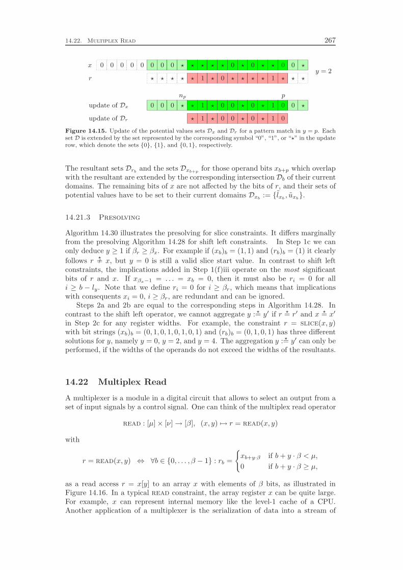
14.22. Multiplex Read 267
00000000
0000
0
000000000000
11
11
11
⋆⋆⋆⋆⋆⋆
⋆ ⋆⋆
⋆⋆⋆⋆
⋆⋆⋆⋆⋆⋆⋆
⋆⋆⋆⋆⋆⋆⋆⋆⋆
⋆⋆ ⋆
x
r
np p
update of Dx
update of Dr
y = 2
Figure 14.15. Update of the potential values sets Dx and Dr for a pattern match in y = p. Eachset D is extended by the set represented by the corresponding symbol “0”, “1”, or “⋆” in the updaterow, which denote the sets {0}, {1}, and {0, 1}, respectively.
The resultant sets Drband the sets Dxb+p
for those operand bits xb+p which overlapwith the resultant are extended by the corresponding intersection Db of their currentdomains. The remaining bits of x are not affected by the bits of r, and their sets ofpotential values have to be set to their current domains Dxb
:= {lxb, uxb}.
14.21.3 Presolving
Algorithm 14.30 illustrates the presolving for slice constraints. It differs marginallyfrom the presolving Algorithm 14.28 for shift left constraints. In Step 1c we canonly deduce y ≥ 1 if βr ≥ βx. For example if (xb)b = (1, 1) and (rb)b = (1) it clearly
follows r Y⋆= x, but y = 0 is still a valid slice start value. In contrast to shift left
constraints, the implications added in Step 1(f)iii operate on the most significantbits of r and x. If xβx−1 = . . . = xb = 0, then it must also be ri = 0 for alli ≥ b − ly. Note that we define ri = 0 for i ≥ βr, which means that implicationswith consequents xi = 0, i ≥ βr, are redundant and can be ignored.
Steps 2a and 2b are equal to the corresponding steps in Algorithm 14.28. Incontrast to the shift left operator, we cannot aggregate y : ⋆= y′ if r ⋆= r′ and x ⋆= x′
in Step 2c for any register widths. For example, the constraint r = slice(x, y)with bit strings (xb)b = (0, 1, 0, 1, 0, 1, 0, 1) and (rb)b = (0, 1, 0, 1) has three differentsolutions for y, namely y = 0, y = 2, and y = 4. The aggregation y : ⋆= y′ can only beperformed, if the widths of the operands do not exceed the widths of the resultants.
14.22 Multiplex Read
A multiplexer is a module in a digital circuit that allows to select an output from aset of input signals by a control signal. One can think of the multiplex read operator
read : [µ]× [ν]→ [β], (x, y) 7→ r = read(x, y)
with
r = read(x, y) ⇔ ∀b ∈ {0, . . . , β − 1} : rb =
{
xb+y·β if b+ y · β < µ,
0 if b+ y · β ≥ µ,
as a read access r = x[y] to an array x with elements of β bits, as illustrated inFigure 14.16. In a typical read constraint, the array register x can be quite large.For example, x can represent internal memory like the level-1 cache of a CPU.Another application of a multiplexer is the serialization of data into a stream of
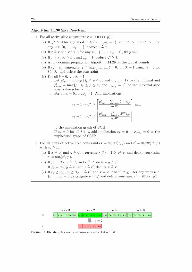
268 Operators in Detail
Algorithm 14.30 Slice Presolving
1. For all active slice constraints r = slice(x, y):
(a) If yw > 0 for any word w ∈ {0, . . . , ωy − 1}, and xw > 0 or rw > 0 for
any w ∈ {0, . . . , ωx − 1}, deduce r Y⋆= x.
(b) If r ⋆= x and xw > 0 for any w ∈ {0, . . . , ωx − 1}, fix y := 0.
(c) If r Y⋆= x, βr ≥ βx, and ωy = 1, deduce y0 ≥ 1.
(d) Apply domain propagation Algorithm 14.29 on the global bounds.
(e) If ly = uy, aggregate rb : ⋆= xb+ly for all b = 0, . . . , βr − 1 using xi = 0 fori ≥ βx, and delete the constraint.
(f) For all b = 0, . . . , βr − 1:i. Let pb
min = min{p | ly ≤ p ≤ uy and uxb+p= 1} be the minimal and
pbmax = max{p | ly ≤ p ≤ uy and uxb+p
= 1} be the maximal slicestart value y for rb = 1.
ii. For all w = 0, . . . , ωy − 1: Add implications
rb = 1→ yw ≥
⌈
pbmin −
∑
i 6=w 2iWuyi
2wW
⌉
and
rb = 1→ yw ≤
⌊
pbmax −
∑
i 6=w 2iW lyi
2wW
⌋
to the implication graph of SCIP.iii. If xi = 0 for all i > b, add implication xb = 0 → rb−ly = 0 to the
implication graph of SCIP.
2. For all pairs of active slice constraints r = slice(x, y) and r′ = slice(x′, y′)with βr ≥ βr′ :
(a) If x ⋆= x′ and y ⋆= y′, aggregate r[βr′ − 1, 0] : ⋆= r′ and delete constraintr′ = shl(x′, y′).
(b) If βr = βr′ , x ⋆= x′, and r Y⋆= r′, deduce y Y
⋆= y′.
If βr = βr′ , y ⋆= y′, and r Y⋆= r′, deduce x Y
⋆= x′.
(c) If βr ≥ βx, βr′ ≥ βx′ , r ⋆= r′, and x ⋆= x′, and if rw ≥ 1 for any word w ∈{0, . . . , ωr − 1}, aggregate y : ⋆= y′ and delete constraint r′ = shl(x′, y′).
x19x18x17x16x15 x14x13x12x11x10 x9 x8 x7 x6 x5 x4 x3 x2 x1 x0
r4 r3 r2 r1 r0
y = 2
block 0block 1block 2block 3
x
r
Figure 14.16. Multiplex read with array elements of β = 5 bits.
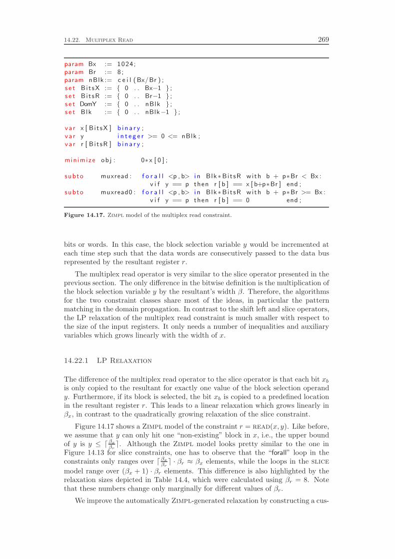
14.22. Multiplex Read 269
param Bx := 1024;param Br := 8 ;param nBlk := c e i l (Bx/Br ) ;s e t Bi t sX := { 0 . . Bx−1 } ;s e t Bi t sR := { 0 . . Br−1 } ;s e t DomY := { 0 . . nBlk } ;s e t Blk := { 0 . . nBlk−1 } ;
va r x [ B i t sX ] b i n a r y ;va r y i n t e g e r >= 0 <= nBlk ;va r r [ B i t sR ] b i n a r y ;
min imize ob j : 0∗x [ 0 ] ;
subto muxread : f o r a l l <p , b> i n Blk∗Bit sR with b + p∗Br < Bx :v i f y == p then r [ b ] == x [ b+p∗Br ] end ;
subto muxread0 : f o r a l l <p , b> i n Blk∗Bit sR with b + p∗Br >= Bx :v i f y == p then r [ b ] == 0 end ;
Figure 14.17. Zimpl model of the multiplex read constraint.
bits or words. In this case, the block selection variable y would be incremented ateach time step such that the data words are consecutively passed to the data busrepresented by the resultant register r.
The multiplex read operator is very similar to the slice operator presented in theprevious section. The only difference in the bitwise definition is the multiplication ofthe block selection variable y by the resultant’s width β. Therefore, the algorithmsfor the two constraint classes share most of the ideas, in particular the patternmatching in the domain propagation. In contrast to the shift left and slice operators,the LP relaxation of the multiplex read constraint is much smaller with respect tothe size of the input registers. It only needs a number of inequalities and auxiliaryvariables which grows linearly with the width of x.
14.22.1 LP Relaxation
The difference of the multiplex read operator to the slice operator is that each bit xb
is only copied to the resultant for exactly one value of the block selection operandy. Furthermore, if its block is selected, the bit xb is copied to a predefined locationin the resultant register r. This leads to a linear relaxation which grows linearly inβx, in contrast to the quadratically growing relaxation of the slice constraint.
Figure 14.17 shows a Zimpl model of the constraint r = read(x, y). Like before,we assume that y can only hit one “non-existing” block in x, i.e., the upper boundof y is y ≤ ⌈βx
βr⌉. Although the Zimpl model looks pretty similar to the one in
Figure 14.13 for slice constraints, one has to observe that the “forall” loop in theconstraints only ranges over ⌈βx
βr⌉ · βr ≈ βx elements, while the loops in the slice
model range over (βx + 1) · βr elements. This difference is also highlighted by therelaxation sizes depicted in Table 14.4, which were calculated using βr = 8. Notethat these numbers change only marginally for different values of βr.
We improve the automatically Zimpl-generated relaxation by constructing a cus-
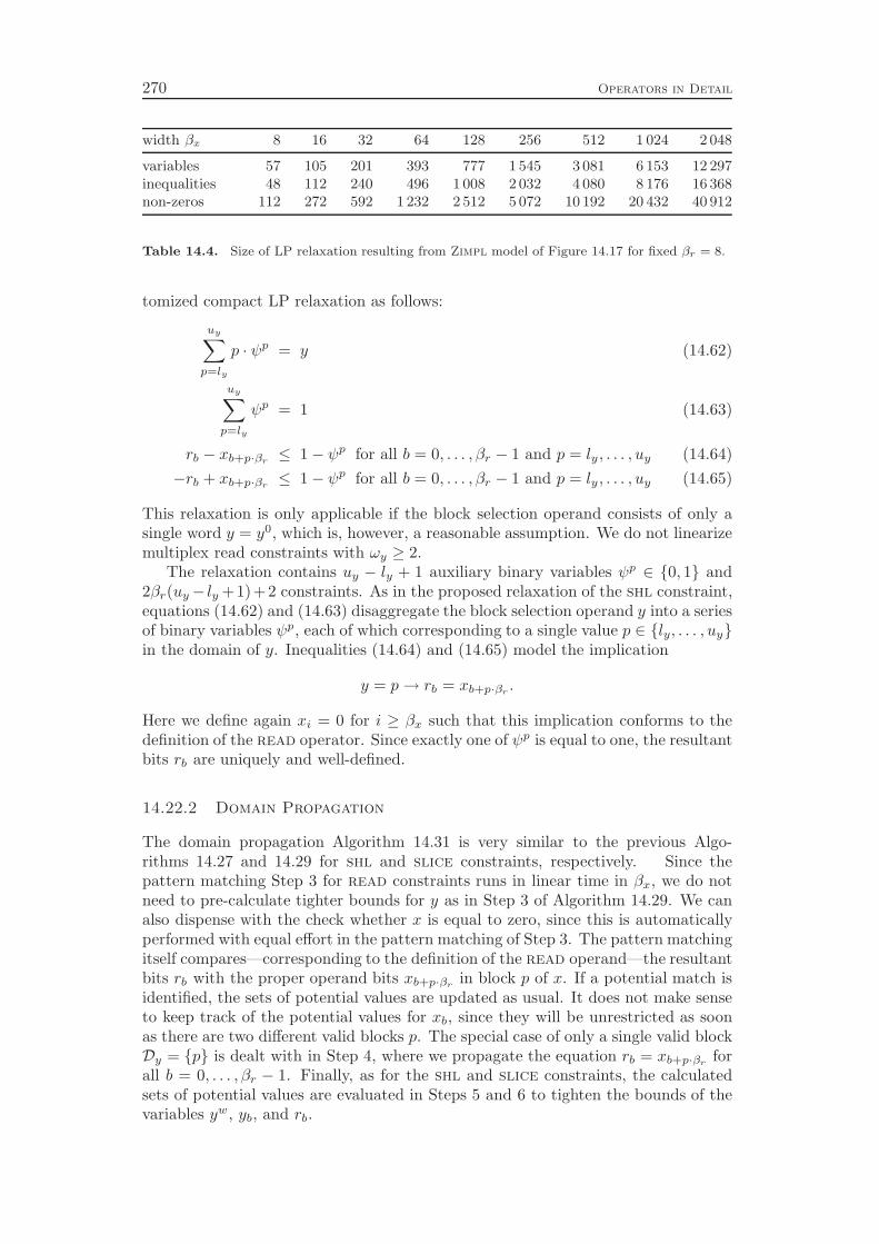
270 Operators in Detail
width βx 8 16 32 64 128 256 512 1 024 2 048
variables 57 105 201 393 777 1 545 3 081 6 153 12 297inequalities 48 112 240 496 1 008 2 032 4 080 8 176 16 368non-zeros 112 272 592 1 232 2 512 5 072 10 192 20 432 40 912
Table 14.4. Size of LP relaxation resulting from Zimpl model of Figure 14.17 for fixed βr = 8.
tomized compact LP relaxation as follows:
uy∑
p=ly
p · ψp = y (14.62)
uy∑
p=ly
ψp = 1 (14.63)
rb − xb+p·βr≤ 1− ψp for all b = 0, . . . , βr − 1 and p = ly , . . . , uy (14.64)
−rb + xb+p·βr≤ 1− ψp for all b = 0, . . . , βr − 1 and p = ly , . . . , uy (14.65)
This relaxation is only applicable if the block selection operand consists of only asingle word y = y0, which is, however, a reasonable assumption. We do not linearizemultiplex read constraints with ωy ≥ 2.
The relaxation contains uy − ly + 1 auxiliary binary variables ψp ∈ {0, 1} and2βr(uy− ly +1)+2 constraints. As in the proposed relaxation of the shl constraint,equations (14.62) and (14.63) disaggregate the block selection operand y into a seriesof binary variables ψp, each of which corresponding to a single value p ∈ {ly, . . . , uy}in the domain of y. Inequalities (14.64) and (14.65) model the implication
y = p→ rb = xb+p·βr.
Here we define again xi = 0 for i ≥ βx such that this implication conforms to thedefinition of the read operator. Since exactly one of ψp is equal to one, the resultantbits rb are uniquely and well-defined.
14.22.2 Domain Propagation
The domain propagation Algorithm 14.31 is very similar to the previous Algo-rithms 14.27 and 14.29 for shl and slice constraints, respectively. Since thepattern matching Step 3 for read constraints runs in linear time in βx, we do notneed to pre-calculate tighter bounds for y as in Step 3 of Algorithm 14.29. We canalso dispense with the check whether x is equal to zero, since this is automaticallyperformed with equal effort in the pattern matching of Step 3. The pattern matchingitself compares—corresponding to the definition of the read operand—the resultantbits rb with the proper operand bits xb+p·βr
in block p of x. If a potential match isidentified, the sets of potential values are updated as usual. It does not make senseto keep track of the potential values for xb, since they will be unrestricted as soonas there are two different valid blocks p. The special case of only a single valid blockDy = {p} is dealt with in Step 4, where we propagate the equation rb = xb+p·βr
forall b = 0, . . . , βr − 1. Finally, as for the shl and slice constraints, the calculatedsets of potential values are evaluated in Steps 5 and 6 to tighten the bounds of thevariables yw, yb, and rb.

14.22. Multiplex Read 271
Algorithm 14.31 Multiplex Read Domain Propagation
Input : Multiplex read constraint r = read(x, y) on registers r, x, and y withcurrent local bit bounds lrb
≤ rb ≤ urb, lxb
≤ xb ≤ uxb, and lyb
≤ yb ≤ uyb,
and current local word bounds lyw ≤ yw ≤ uyw .
Output : Tightened local bounds for bits rb, xb, and yb, and words yw.
1. Calculate bounds for the register y from the words’ bounds:
ly :=
ωy−1∑
w=0
2wW lyw and uy :=
ωy−1∑
w=0
2wW uyw .
2. Initialize Drb:= ∅ for all b = 0, . . . , βr − 1, Dyb
:= ∅ for all b = 0, . . . , βy − 1,and Dy := ∅.
3. For all p = ly, . . . , uy :
Let p =∑βy−1
b=0 2bpb be the bit decomposition of p. If the following holds:
(a) pb ∈ {lyb, uyb} for all b = 0, . . . , βy − 1,
(b) Db := {lrb, urb} ∩ {lxb+p·βr
, uxb+p·βr} 6= ∅ for all b = 0, . . . , βr − 1, and
(c) there is no bit b ∈ {0, . . . , βr − 1} with rb Y⋆= xb+p·βr
,
the block selection value y = p is valid. In this case, update
(a) Dy := Dy ∪ {p},
(b) Dyb:= Dyb
∪ {pb} for all b = 0, . . . , βy − 1, and
(c) Drb:= Drb
∪ Db for all b = 0, . . . , βr − 1.
4. If Dy = {p}, then for all b = 0, . . . , βr − 1:
(a) If lrb= urb
, deduce xb+p·βr= lrb
.
(b) If lxb+p·βr= uxb+p·βr
, deduce rb = lxb+p·βr.
5. Tighten word bounds of yw, w = 0, . . . , ωy − 1, corresponding to the registerbounds min{Dy} ≤ y ≤ max{Dy}.
6. For all b = 0, . . . , βy − 1: Tighten min{Dyb} ≤ yb ≤ max{Dyb
}.For all b = 0, . . . , βr − 1: Tighten min{Drb
} ≤ rb ≤ max{Drb}.
14.22.3 Presolving
Like the domain propagation, the presolving for multiplex read constraints does notdiffer much from the presolving of slice constraints. Algorithm 14.32 illustrates theprocedure. We do not apply Step 1c of Algorithm 14.30. Although the reasoningis valid for read constraints as well, the condition βr ≥ βx will never be satisfied,since in every reasonable multiplexer the array x has more bits than the resultant r.Of course, the aggregations in Step 1d and the calculations in Step 1(e)i are adaptedto the definition of the read operator. Due to the blockwise selection of the inputbits xb by the operand y we cannot generate implications like the ones of Step 1(f)iiiof Algorithm 14.30.
Pairs of read constraints are only compared in Step 2 if their resultants havethe same width. Otherwise, the partitioning of x into blocks would be different andthe values of the block selection operands y and y′ would have different meaning.
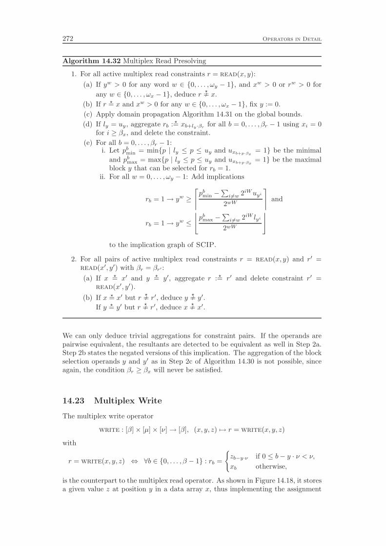
272 Operators in Detail
Algorithm 14.32 Multiplex Read Presolving
1. For all active multiplex read constraints r = read(x, y):
(a) If yw > 0 for any word w ∈ {0, . . . , ωy − 1}, and xw > 0 or rw > 0 for
any w ∈ {0, . . . , ωx − 1}, deduce r Y⋆= x.
(b) If r ⋆= x and xw > 0 for any w ∈ {0, . . . , ωx − 1}, fix y := 0.
(c) Apply domain propagation Algorithm 14.31 on the global bounds.
(d) If ly = uy , aggregate rb : ⋆= xb+ly ·βrfor all b = 0, . . . , βr − 1 using xi = 0
for i ≥ βx, and delete the constraint.
(e) For all b = 0, . . . , βr − 1:i. Let pb
min = min{p | ly ≤ p ≤ uy and uxb+p·βx= 1} be the minimal
and pbmax = max{p | ly ≤ p ≤ uy and uxb+p·βx
= 1} be the maximalblock y that can be selected for rb = 1.
ii. For all w = 0, . . . , ωy − 1: Add implications
rb = 1→ yw ≥
⌈
pbmin −
∑
i 6=w 2iWuyi
2wW
⌉
and
rb = 1→ yw ≤
⌊
pbmax −
∑
i 6=w 2iW lyi
2wW
⌋
to the implication graph of SCIP.
2. For all pairs of active multiplex read constraints r = read(x, y) and r′ =read(x′, y′) with βr = βr′ :
(a) If x ⋆= x′ and y ⋆= y′, aggregate r : ⋆= r′ and delete constraint r′ =read(x′, y′).
(b) If x ⋆= x′ but r Y⋆= r′, deduce y Y
⋆= y′.
If y ⋆= y′ but r Y⋆= r′, deduce x Y
⋆= x′.
We can only deduce trivial aggregations for constraint pairs. If the operands arepairwise equivalent, the resultants are detected to be equivalent as well in Step 2a.Step 2b states the negated versions of this implication. The aggregation of the blockselection operands y and y′ as in Step 2c of Algorithm 14.30 is not possible, sinceagain, the condition βr ≥ βx will never be satisfied.
14.23 Multiplex Write
The multiplex write operator
write : [β]× [µ]× [ν]→ [β], (x, y, z) 7→ r = write(x, y, z)
with
r = write(x, y, z) ⇔ ∀b ∈ {0, . . . , β − 1} : rb =
{
zb−y·ν if 0 ≤ b− y · ν < ν,
xb otherwise,
is the counterpart to the multiplex read operator. As shown in Figure 14.18, it storesa given value z at position y in a data array x, thus implementing the assignment
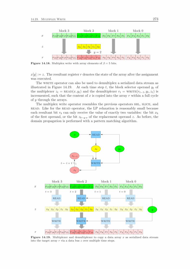
14.23. Multiplex Write 273
x19x18x17x16x15 x14x13x12x11x10 x9 x8 x7 x6 x5 x4 x3 x2 x1 x0
z4 z3 z2 z1 z0
y = 2
r19 r18 r17 r16 r15 r14 r13 r12 r11 r10 r9 r8 r7 r6 r5 r4 r3 r2 r1 r0
block 0block 1block 2block 3
x
z
r
Figure 14.18. Multiplex write with array elements of β = 5 bits.
x[y] := z. The resultant register r denotes the state of the array after the assignmentwas executed.
The write operator can also be used to demultiplex a serialized data stream asillustrated in Figure 14.19. At each time step t, the block selector operand yt ofthe multiplexer zt = read(x, yt) and the demultiplexer rt = write(rt−1, yt, zt) isincremented, such that the content of x is copied into the array r within a full cycleof y through the arrays.
The multiplex write operator resembles the previous operators shl, slice, andread. Like for the read operator, the LP relaxation is reasonably small becauseeach resultant bit rb can only receive the value of exactly two variables: the bit xb
of the first operand, or the bit zb−y·ν of the replacement operand z. As before, thedomain propagation is performed with a pattern matching algorithm.
x19x18x17x16x15 x14x13x12x11x10 x9 x8 x7 x6 x5 x4 x3 x2 x1 x0
z4z4z4z4 z3z3z3z3 z2z2z2z2 z1z1z1z1 z0z0z0z0
r19 r18 r17 r16 r15 r14 r13 r12 r11 r10 r9 r8 r7 r6 r5 r4 r3 r2 r1 r0
block 0block 1block 2block 3
x
x
z
r
y
ytzt
rt
rt−1
t← t + 1
t = 0t = 1t = 2t = 3
read read readread
read
writewritewrite write
write
Figure 14.19. Multiplexer and demultiplexer to copy a data array x as serialized data streaminto the target array r via a data bus z over multiple time steps.
274 Operators in Detail
14.23.1 LP Relaxation
Analogously to the read operator relaxation, we define the relaxation of writeconstraints as follows:
uy∑
p=ly
p · ψp = y (14.66)
uy∑
p=ly
ψp = 1 (14.67)
rb+p·βz− zb ≤ 1− ψp for all b = 0, . . . , βz − 1 and p = ly, . . . , uy (14.68)
−rb+p·βz + zb ≤ 1− ψp for all b = 0, . . . , βz − 1 and p = ly, . . . , uy (14.69)
rb+p·βz− xb+p·βz
≤ ψp for all b = 0, . . . , βz − 1 and p = ly, . . . , uy (14.70)
−rb+p·βz+ xb+p·βz
≤ ψp for all b = 0, . . . , βz − 1 and p = ly, . . . , uy (14.71)
As before, by equations (14.66) and (14.67) we split the block selection operand yinto a series of binary variables ψp ∈ {0, 1}, each of which represents one value inthe domain y ∈ {ly, . . . , uy}. For this being valid, we assume that y = y0 consistsof only one word, i.e., ωy = 1. We do not linearize multiplex write constraints withωy ≥ 2.
Inequalities (14.68) to (14.71) model the constraint rb+p·βz= ite(ψp, zb, xb+p·βz
),compare the LP relaxation of if-then-else constraints in Section 14.15.1. The firsttwo inequalities ensure
ψp = 1→ rb+p·βz= zb,
while the latter two force
ψp = 0→ rb+p·βz= xb+p·βz
.
Note that the bits in the blocks p < ly or p > uy that cannot be selected byvariable y are aggregated as rb+p·βz
: ⋆= xb+p·βzfor b = 0, . . . , βz − 1 in Step 1(b)iii
of the presolving Algorithm 14.34. Thus, we do not need additional inequalities oftypes (14.70) and (14.71) for p /∈ {ly, . . . , uy}.
14.23.2 Domain Propagation
The domain propagation Algorithm 14.33 for multiplex write constraints is some-what different than the one for the read operator. After the bounds for the blockselection operand y are calculated as usual in Step 1, we perform a first check inStep 2 whether there is an inconsistency of bits rb 6= xb in block p =
⌊b
βz
⌋. In this
situation rb must have been overwritten by z, and y can therefore be fixed to p.The pattern matching of Step 4 runs as usual with the additional update 4d: if
the overlapping bits zb and xi, i = b+ p · βz, for block p are fixed to the same value,the corresponding resultant bit ri must also take this value. In the special case thatonly one possible matching Dy = {p} was found, we can propagate rb+p·βz
= zb inStep 5 for all b = 0, . . . , βz − 1. Step 6 processes all blocks where z does not matchto the corresponding part of r. For the bits b in these blocks it must be rb = xb.Finally, Steps 7 and 8 apply our knowledge about the potential values of y, yb, andzb to tighten the corresponding word and bit variables.

14.23. Multiplex Write 275
Algorithm 14.33 Multiplex Write Domain Propagation
Input : Multiplex write constraint r = write(x, y, z) on registers r, x, y, and zwith current local bit bounds lrb
≤ rb ≤ urb, lxb≤ xb ≤ uxb
, and lyb≤ yb ≤
uyb, and lzb
≤ zb ≤ uzb, and current local word bounds lyw ≤ yw ≤ uyw .
Output : Tightened local bounds for bits rb, xb, yb, and zb, and words yw.
1. Calculate bounds for the register y from the words’ bounds:
ly :=
ωy−1∑
w=0
2wW lyw and uy :=
ωy−1∑
w=0
2wW uyw .
2. For all b = 0, . . . , βr − 1:If lrb
> uxb, urb
< lxb, or rb Y
⋆= xb, set ly := uy := ⌊ b
βz⌋ and abort the loop.
3. Initialize Dzb:= ∅ for all b = 0, . . . , βz − 1, Dyb
:= ∅ for all b = 0, . . . , βy − 1,and Dy := ∅.
4. For all p = ly, . . . , uy :
Let p =∑βy−1
b=0 2bpb be the bit decomposition of p. If the following holds:
(a) pb ∈ {lyb, uyb} for all b = 0, . . . , βy − 1,
(b) Db := {lrb+p·βz, urb+p·βz
} ∩ {lzb, uzb} 6= ∅ for all b = 0, . . . , βz − 1, and
(c) there is no bit b ∈ {0, . . . , βz − 1} with rb+p·βzY⋆= zb,
the block selection value y = p is valid. In this case, update
(a) Dy := Dy ∪ {p},
(b) Dyb:= Dyb
∪ {pb} for all b = 0, . . . , βy − 1,
(c) Dzb:= Dzb
∪ Db for all b = 0, . . . , βz − 1, and
(d) if lzb= uzb
= lxb+p·βz= uxb+p·βz
, deduce rb+p·βz= lzb
.
5. If Dy = {p}, then for all b = 0, . . . , βz − 1:
(a) If lzb= uzb
, deduce rb+p·βz= lzb
.
(b) If lrb+p·βz= urb+p·βz
, deduce zb = lrb+p·βz.
6. For all b = 0, . . . , βr − 1 with⌊
bβz
⌋/∈ Dy:
(a) If lxb= uxb
, deduce rb = lxb.
(b) If lrb= urb
, deduce xb = lrb.
7. Tighten word bounds of yw, w = 0, . . . , ωy − 1, corresponding to the registerbounds min{Dy} ≤ y ≤ max{Dy}.
8. For all b = 0, . . . , βy − 1: Tighten min{Dyb} ≤ yb ≤ max{Dyb
}.For all b = 0, . . . , βz − 1: Tighten min{Dzb
} ≤ zb ≤ max{Dzb}.

276 Operators in Detail
Algorithm 14.34 Multiplex Write Presolving
1. For all active multiplex write constraints r = write(x, y):
(a) If r ⋆= z, zw > 0 for any w ∈ {0, . . . , ωz − 1}, and uy <⌈
βr
βz
⌉, fix y := 0.
(b) Apply domain propagation Algorithm 14.33 on the global bounds withthe following modifications:
i. Instead of Update 4d, if xb+p·βz
⋆= zb, aggregate rb+p·βz: ⋆= zb.
ii. In Step 5, aggregate rb+p·βz: ⋆= zb instead of only deducing bounds.
iii. In Step 6, aggregate rb : ⋆= xb instead of only deducing bounds.
(c) For all p = ly, . . . , uy and all b = 0, . . . , βz−1, define j = b+p·βz to be thecorresponding bit position in x and r, and add the following implicationsto the implication graph of SCIP:
i. If xj = 0, add implications rj = 1→ zb = 1 and rj = 1→ y = p.If xj = 1, add implications rj = 0→ zb = 0 and rj = 0→ y = p.
ii. If rj = 0, add implications xj = 1→ zb = 0 and xj = 1→ y = p.If rj = 1, add implications xj = 0→ zb = 1 and xj = 0→ y = p.
iii. If zb = 0, add implication xj = 0→ rj = 0.If zb = 1, add implication xj = 1→ rj = 1.
iv. If rj = 0, p = ly, and ωy = 1, add implication zb = 1→ y ≥ ly + 1.If rj = 1, p = ly, and ωy = 1, add implication zb = 0→ y ≥ ly + 1.If rj = 0, p = uy, and ωy = 1, add implication zb = 1→ y ≤ uy − 1.If rj = 1, p = uy, and ωy = 1, add implication zb = 0→ y ≤ uy − 1.
v. If zb = 0, p = ly, and ωy = 1, add implication rj = 1→ y ≥ ly + 1.If zb = 1, p = ly, and ωy = 1, add implication rj = 0→ y ≥ ly + 1.If zb = 0, p = uy, and ωy = 1, add implication rj = 1→ y ≤ uy − 1.If zb = 1, p = uy, and ωy = 1, add implication rj = 0→ y ≤ uy − 1.
2. For all pairs of active multiplex write constraints r = write(x, y, z) and r′ =write(x′, y′, z′) with βz = βz′ and βr ≥ βr′ :
(a) If x ⋆= x′, y ⋆= y′, and z ⋆= z′, aggregate r[βr′ − 1, 0] : ⋆= r′ and delete theconstraint r′ = write(x′, y′, z′).
(b) If βr = βr′ , x ⋆= x′, y ⋆= y′, but r Y⋆= r′, deduce z Y
⋆= z′.
If βr = βr′ , x ⋆= x′, z ⋆= z′, but r Y⋆= r′, deduce y Y
⋆= y′.
If βr = βr′ , y ⋆= y′, z ⋆= z′, but r Y⋆= r′, deduce x Y
⋆= x′.
(c) If r ⋆= r′, y ⋆= y′, and uy <⌈
min{βr ,β′r}
βz
⌉
, aggregate z : ⋆= z′.
(d) If z Y⋆= z′, y ⋆= y′, and uy <
⌈min{βr ,β′
r}βz
⌉
, deduce r Y⋆= r′.
14.23.3 Presolving
The presolving of multiplex write constraints as depicted in Algorithm 14.34 startsby checking in Step 1a whether the resultant is equivalent to the write operand z. Ifthe latter is non-zero, and if the upper bound of the block selection operand y ensuresthat the complete bit string of z is written into r, z must be written into block 0 ofr, and we can fix y := 0. The main part of the algorithm consists of calling thedomain propagation Algorithm 14.33 on the global bounds in Step 1b. However,we replace the steps that propagate the equality of two registers by a correspondingaggregation. Step 1c considers all potential values of the block selection operand yand identifies implications that can be added to the implication graph of SCIP. If
14.23. Multiplex Write 277
xj , zb, and rj are the bits that belong together in the current block p, Steps 1(c)ito 1(c)iii apply the implication
xj 6= rj → rj = zb ∧ y = p (14.72)
for all fixings of a single variable. In particular, the implication xj = zb → rj = xj
used in Step 1(c)iii follows from (14.72), since
(xj = zb) ∧ (xj 6= rj → rj = zb) ⇒ (xj 6= rj → rj = xj) ⇒ rj = xj .
Steps 1(c)iv and 1(c)v apply the same implication reorganized to the form
rj 6= zb → y 6= p.
Such an inequality y 6= p (which is a disjunction y < p ∨ y > p) in the conclusionof an implication cannot be stored in the implication graph of SCIP. Therefore, wecan only exploit this situation in the blocks p corresponding to the lower and upperbounds of the block selection variable y, where the inequality becomes y ≤ p− 1 ory ≥ p+ 1, respectively. Additionally, we can only use these implications if the blockselection operand consists of only a single word. Otherwise, the conclusion wouldbe a disjunction on the different word variables yw.
The pairwise presolving of Step 2 can only be applied for write constraintsof equal βz. Otherwise, the partitioning of x and r into array elements would bedifferent. Step 2a applies the trivial aggregation which states that two constraintswith equivalent operands must have equivalent resultant bits. Step 2b executes thisrule in the inverse direction. Step 2c is a bit more interesting: if the resultants andthe block selection operands are pairwise equivalent, we can deduce that the writtenvalue z must also be equivalent. This is, however, only true if z would be absorbedcompletely by r, i.e., if the upper bound of the block selection operand y is smallenough. The inverse implication of this rule is stated in Step 2d: if unequal valuesare written to the same position, and if all of these bits will affect the resultants,the resultants must be unequal.


Chapter 15
Presolving
In the previous chapter, we presented the algorithms used in the constraint han-dlers of our property checking tool to process the different circuit operators. Oneimportant ingredient of a constraint handler is the presolving component. Theseconstraint based presolving algorithms try to simplify the problem instance by con-sidering the constraints of a single constraint class independently from all otherconstraints. Even more, most of the reductions are deduced from a single constraintand the bounds of the involved variables. The only “global” information exploitedis our knowledge about the equality or inequality of variables and—to a smallerextent—the discovered implications between the variables which are stored in theimplication graph, see Section 3.3.5.
In addition to the presolving of linear constraints and its specializations, Chap-ter 10 introduced a few general purpose presolving techniques that can be appliedindependent of an individual constraint class. They can be used not only for mixedinteger programs but for any constraint integer program. These concepts, in par-ticular probing and implication graph analysis, are also employed here. In the fol-lowing, we present two additional presolving techniques that are specifically tailoredto the property checking problem. The term algebra preprocessing features a termreplacement system to exploit the commutativity, associativity, and distributivityof the arithmetic constraints add and mult. The irrelevance detection discardsparts of the circuit that are not relevant for the property at hand. This does nothelp to tighten the domains of the variables but reduces the effort spent on theindividual subproblems during the solving process. Furthermore, removing irrele-vant constraints and variables can help the branching strategy to concentrate onthe relevant part on the circuit where the crucial decisions have to be taken, seeSection 16.1.
As described in Section 3.2.5, the preprocessing algorithms of the constraintsand the global presolving algorithms are applied periodically until no more problemreductions can be found. Whenever a new fixing, aggregation, domain reduction, orimplication was found by one of the preprocessing algorithms, presolving is appliedagain to the affected constraints. More expensive presolving operations like probingor term algebra preprocessing are delayed until the other algorithms failed to producefurther reductions.
15.1 Term Algebra Preprocessing
Analog to the symbolic propagation with term rewriting applied in the domain prop-agation of multiplication constraints, see Section 14.5.2, we employ a term rewritingsystem as a global presolving engine. Recall that the symbolic propagation for mul-tiplication constraints was defined on a simple signature consisting of binary variablesymbols B and the operations ∧ : B × B → B and ⊕ : B × B → B. In contrast,the term algebra preprocessing operates on a more complex signature of low signifi-
279
280 Presolving
cant register subwords, truncated addition, and truncated multiplication operators.The goal is to exploit the commutativity, associativity, and distributivity of the twooperators in order to identify equivalent subword-defining terms, thereby concludingthat the subwords themselves must be equivalent.
We need the following preliminaries to justify the term rewriting rules that wewant to employ. A comprehensive introduction on group and ring theory can befound in Allenby [9].
Definition 15.1 (ring homomorphism). If (R,+R, ·R) and (S,+S , ·S) are rings,a ring homomorphism is a mapping f : R→ S such that
1. f(a+R b) = f(a) +S f(b) for all a, b ∈ R, and
2. f(a ·R b) = f(a) ·S f(b) for all a, b ∈ R.
A ring homomorphism f : R→ S on unitary rings (R,+R, ·R, 1R) and (S,+S , ·S , 1S)which satisfies
3. f(1R) = 1S
is called unitary ring homomorphism.
Proposition 15.2. For all n,m ∈ Z>0 with nm∈ Z, the modulus operation
mod m : Zn → Zm, a 7→ a mod m
is a unitary ring homomorphism from the unitary ring (Zn,+n, ·n, 1) to the unitaryring (Zm,+m, ·m, 1) with Zk = {0, . . . , k − 1}, a+k b = (a+ b) mod k, and a ·k b =(a · b) mod k.
Proof. To show Conditions 1 and 2 of Definition 15.1, let ◦ ∈ {+, ·} be either mul-tiplication or addition. Let a, b ∈ Zn and c = (a ◦n b) = (a ◦ b) mod n. Define k ∈ Zto be the unique value with a ◦ b = c + kn. Let a′ = a mod m, b′ = b mod m, andc′ = c mod m. We have to show c′ = a′ ◦m b′. Let p, q, r ∈ Z be the unique valuessuch that a = a′ + pm, b = b′ + qm, and c = c′ + rm. Then, for ◦ = + we have
c′ = c− rm = a+ b− kn− rm = a′ + b′ +(p+ q − k
n
m− r)m = a′ +m b′,
and for ◦ = · it follows
c′ = c− rm = a · b− kn− rm = a′ · b′ +(pq + aq + bp− k
n
m− r)m = a′ ·m b′,
since nm∈ Z by assumption and c′ ∈ Zm. The validity of Condition 3 is obvious.
Corollary 15.3. Truncated addition and truncated multiplication respect the sub-word property, i.e.,
r = add(x, y) ⇒ r[b, 0] = add(x[b, 0], y[b, 0])
r = mult(x, y) ⇒ r[b, 0] = mult(x[b, 0], y[b, 0])
for all b = 0, . . . , βr − 1.
15.1. Term Algebra Preprocessing 281
Our term rewriting system operates on terms composed of the constants 0 and1, the register bits jb and their negations ¯jb, the concatenations of these constantsymbols into bit strings, the truncation of bit strings to shorter strings, and the addand mult operators. In order to obtain a finite signature, we impose a maximumβmax ∈ Z>0 on the width of the bit strings on which the operators are defined. Onecan think of βmax as the maximal width of the registers contained in the propertychecking instance at hand.
Definition 15.4 (bit string arithmetics signature). Let βmax ∈ Z>0 and B ={1, . . . , βmax}. The algebraic signature Σ = (S,O) with the sorts S = {[β] |β ∈ B}and the following operators O = O0 ∪O1 ∪O2:
O0: 0 : → [1]
1 : → [1]
jb : → [1] with j = 1, . . . , n and b = 0, . . . , βj− 1
¯jb : → [1] with j = 1, . . . , n and b = 0, . . . , βj− 1
O1: −β : [β]→ [β]
|βµ: [µ]→ [β] with β, µ ∈ B and µ ≥ β
O2: ⊗βµ : [β − µ]× [µ]→ [β] with β, µ ∈ B and β > µ
· β : [β]× [β]→ [β] with β ∈ B
+β : [β]× [β]→ [β] with β ∈ B
is called bit string arithmetics signature. We call TΣ the term algebra of Σ, whichconsists of all terms that can be generated from the symbols in Σ and which fit tothe arity of the operators. The terms of sort [β] are denoted by T[β]. Thus, T[β]
contains all terms t ∈ TΣ whose outermost operator has codomain [β].
Whenever it is non-ambiguous, we will omit the domain subscripts of the oper-ators. We want to interpret the bit string arithmetics signature to be in line withthe definition of the circuit operators. In particular, the signature operators −, |β ,⊗, · , and + should reflect the properties of the minus, slice( · , 0), concat, mult,and add operators, respectively. Formally, we have to introduce equations E to thesignature Σ in order to describe the relevant properties of the circuit operators. Westart with the associative law, which is valid for the three binary operators:
tν ⊗ (tµ ⊗ tβ) = (tν ⊗ tµ)⊗ tβ
tβ3 · (tβ2 · t
β1 ) = (tβ3 · t
β2 ) · tβ1
tβ3 + (tβ2 + tβ1 ) = (tβ3 + tβ2 ) + tβ1
(15.1)
Here we have tβ, tβi ∈ T[β], tµ ∈ T[µ], and tν ∈ T[ν]. These equations allow to simplify
the notation by removing the brackets with the implicit meaning that the operatorsfrom left to right represent innermost to outermost operations. Now we extend

282 Presolving
system (15.1) by the following equations to yield the final set of equations E:
−(−tβ) = tβ
(cµ−1 ⊗ · · · ⊗ c0)|β = cβ−1 ⊗ · · · ⊗ c0
tβ · (0⊗ · · · ⊗ 0) = 0⊗ · · · ⊗ 0
tβ · (0⊗ · · · ⊗ 0⊗ 1) = tβ
tβ1 · (tβ−12 ⊗ 0) = (tβ1 |β−1 · t
β−12 )⊗ 0
tβ1 · tβ2 = tβ2 · t
β1
(tβ3 · tβ1 ) · tβ2 = (tβ3 · t
β2 ) · tβ1
(tµ2 · tµ1 )|β = (tµ2 |β) · (tµ1 |β)
tβ2 · (−tβ1 ) = −(tβ2 · t
β1 )
(−tβ2 ) · tβ1 = −(tβ2 · tβ1 )
− (0⊗ · · · ⊗ 0) = 0⊗ · · · ⊗ 0
(−tβ)⊗ 0 = − (tβ ⊗ 0)
tβ + (0⊗ · · · ⊗ 0) = tβ
(tβ1 + tβ2 )⊗ 0 = (tβ1 ⊗ 0) + (tβ2 ⊗ 0)
tβ1 + tβ2 = tβ2 + tβ1
(tβ3 + tβ1 ) + tβ2 = (tβ3 + tβ2 ) + tβ1(tµ2 + tµ1 )|β = (tµ2 |β) + (tµ1 |β)
tβ + (−tβ) = 0⊗ · · · ⊗ 0
tβ3 · (tβ2 + tβ1 ) = (tβ3 · t
β2 ) + (tβ3 · t
β1 )
(tβ3 + tβ2 ) · tβ1 = (tβ3 · tβ1 ) + (tβ2 · t
β1 )
with ci ∈ O0 being constant symbols. These equations define an equivalence relation≡E ⊆ TΣ × TΣ which identifies terms s ≡E t, s, t ∈ TΣ, that would always yield thesame results when evaluated with circuit operators. We can apply these equationsto terms t ∈ TΣ in order to transform them into normal form.
Definition 15.5 (normal form). We call a term t ∈ T[β] to be in normal form ifit has the form
t = (am + . . . + a1)
with ai = [−]((fimi
· . . . · fi1)⊗ 0⊗ · · · ⊗ 0︸ ︷︷ ︸
si times
)for i = 1, . . . ,m,
and fij = cij,β−si−1 ⊗ · · · ⊗ cij,0 for i = 1, . . . ,m, and j = 1, . . . ,mi
with si ∈ {0, . . . , β − 1}, cij,k ∈ O0, cij,0 6= 0, i = 1, . . . ,m, j = 1, . . . ,mi, k =0, . . . , β − si − 1. The minus symbol enclosed in brackets [−] is optional.
Note. Observe that the number si of appended “⊗ 0”s may be zero, which meansthat no “⊗” operator is contained in ai.
Note. We cannot transform all terms t ∈ TΣ into normal form using equations E.For example, no equation can be applied on the term t = (1 + 1) ⊗ 1, although itis not in normal form. In our presolving algorithm, however, we will only produceterms that can be transformed into normal form.
The normalization of a term t ∈ TΣ is accomplished by executing term rewritingrules R = {le → re | e ∈ E} in an arbitrary order until no more rules are applicable,see Algorithm 15.1. In this definition, le and re are the left and right hand sides ofthe equations e ∈ E. In order to ensure the termination of this rewriting process,we have to restrict the use of the commutativity Rules 2e, 2f, 3d, and 3e. Let ≻ be

15.1. Term Algebra Preprocessing 283
Algorithm 15.1 Term Algebra Preprocessing – Term Normalization
Input : Term t ∈ TΣOutput : Term t′ ≡E t in normal form
Apply the following subterm rewriting rules in any order until no more rules areapplicable, with tk, tki ∈ T[β], and ci ∈ O0 being subterms of t:
1. Minus, Truncation, and Concatenation:
(a) −(− tβ
)→ tβ
(b) − (0⊗ · · · ⊗ 0) → 0⊗ · · · ⊗ 0
(c)(− tβ
)⊗ 0 → −
(tβ ⊗ 0
)
(d)(cµ−1 ⊗ · · · ⊗ c0
)|β → cβ−1 ⊗ · · · ⊗ c0
(e) tν ⊗(tµ ⊗ tβ
)→(tν ⊗ tµ
)⊗ tβ
2. Multiplication:
(a) tβ3 ·(tβ2 · t
β1
)→(tβ3 · t
β2
)· tβ1
(b) tβ ·(0⊗ · · · ⊗ 0
)→ 0⊗ · · · ⊗ 0
(c) tβ ·(0⊗ · · · ⊗ 0⊗ 1
)→ tβ
(d) tβ1 ·(tβ−12 ⊗ 0
)→(tβ1 |β−1 · t
β−12
)⊗ 0
(e) tβ1 · tβ2 → tβ2 · t
β1
(if tβ2 ≻lrpo t
β1
)
(f)(tβ3 · t
β1
)· tβ2 →
(tβ3 · t
β2
)· tβ1
(if tβ2 ≻lrpo t
β1
)
(g)(tµ2 · t
µ1
)|β → tµ2 |β · t
µ1 |β
(h) tβ2 ·(− tβ1
)→ −
(tβ2 · t
β1
)
(i)(− tβ2
)· tβ1 → −
(tβ2 · t
β1
)
3. Addition:
(a) tβ3 +(tβ2 + tβ1
)→(tβ3 + tβ2
)+ tβ1
(b) tβ +(0⊗ · · · ⊗ 0
)→ tβ
(c)(tβ1 + tβ2
)⊗ 0 →
(tβ1 ⊗ 0
)+(tβ2 ⊗ 0
)
(d) tβ1 + tβ2 → tβ2 + tβ1(if tβ2 ≻lrpo t
β1
)
(e)(tβ3 + tβ1
)+ tβ2 →
(tβ3 + tβ2
)+ tβ1
(if tβ2 ≻lrpo t
β1
)
(f)(tµ2 + tµ1
)|β → tµ2 |β + tµ1 |β
(g) tβ +(− tβ
)→ 0⊗ · · · ⊗ 0
4. Distributivity:
(a) tβ3 ·(tβ2 + tβ1
)→ tβ3 · t
β2 + tβ3 · t
β1
(b)(tβ3 + tβ2
)· tβ1 → tβ3 · t
β1 + tβ2 · t
β1
284 Presolving
the precedence relation defined as the transitive closure of
µ > β ⇒ ◦µ ≻ •β for all ◦, • ∈ {|·, · ,⊗,−,+},
|β ≻ · β ≻ ⊗β ≻ −β ≻ +β for all β ∈ B \ {1},
|1 ≻ · 1 ≻ −1 ≻ +1 ≻ ¯jb ≻ j′b′ ≻ 1 ≻ 0,
|βµ≻ |βν
⇔ µ > ν,
⊗βµ ≻ ⊗βν ⇔ µ > ν,
¯jb ≻ ¯j′b′
jb ≻ j′b′
}
⇔ j > j′ ∨ (j = j′ ∧ b > b′)
(15.2)
As in the termination proof of the binary multiplication term normalization Algo-rithm 14.9, see Section 14.5.2, we define ≻lrpo to be the lexicographic recursive pathordering of Σ with respect to ≻. Recall that ≻lrpo is defined in Definition 14.17 as
g(tn, . . . , t1) ≻lrpo f(sm, . . . , s1)
⇔ (i) tj �lrpo f(sm, . . . , s1) for some j ∈ {1, . . . , n}, or
(ii) g ≻ f and g(tn, . . . , t1) ≻lrpo si for all i ∈ {1, . . . ,m}, or
(iii) g = f, g(tn, . . . , t1) ≻lrpo si for all i ∈ {1, . . . ,m},
and (tn, . . . , t1) (≻lrpo)lex (sm, . . . , s1)
Now, the commutativity rules are only applicable if tβ2 ≻lrpo tβ1 . In order to treat
Rule 3g in the termination proof below, we need the following lemma:
Lemma 15.6. For all β, µ ∈ B, µ ≥ β, and all t ∈ T[µ] the relation t �lrpo 0⊗· · ·⊗0 ∈T[β] is valid.
Proof. Let d(t) ∈ Z≥0 be the depth of the tree representation of term t. We provethe claim by induction on β and on d(t). For t = 0⊗· · ·⊗ 0 ∈ T[β] nothing has to beshown. Thus, let T ′[µ] = T[µ] \ {0 ⊗ · · · ⊗ 0} and consider t ∈ T ′[µ]. We have to showthat t ≻lrpo 0⊗ · · · ⊗ 0 ∈ T[β].
Assume β = 1 and let µ ≥ β be arbitrary. Because t 6= 0 it follows t ≻lrpo 0 dueto Condition (ii) of Definition 14.17 since 0 is the smallest symbol with respect to≻.
Now let µ ≥ β ≥ 2. Assume that we have already shown the claim for all β′ < βon arbitrary terms t and for all β′ = β on all terms t′ with d(t′) < d(t).
Suppose the outermost operation of t is “⊗”, i.e., t = t2 ⊗ t1 with t1 ∈ T[µ1],t2 ∈ T[µ2], and µ1 + µ2 = µ. Then we have t2 ⊗ t1 ≻lrpo (0 ⊗ · · · ⊗ 0) ⊗ 0 ∈ T[β]
by Condition (iii) of Definition 14.17 since t2 ⊗ t1 ≻lrpo 0 ∈ T[1] and t2 ⊗ t1 ≻lrpo
0⊗ · · · ⊗ 0 ∈ T[β−1] by induction and (t2, t1) (≻lrpo)lex (0⊗ · · · ⊗ 0, 0) because eithert1 6= 0 and therefore t1 ≻lrpo 0 or t2 ∈ T
′[µ−1] and therefore t2 ≻lrpo 0⊗· · ·⊗0 ∈ T[β−1]
by induction.If “⊗” is not the outermost operation of t, we either have t = −t1, t = t1|µ, t =
t1 · t2, or t = t1 + t2 with t1, t2 ∈ T[ν] and ν ≥ µ. In all cases, t ≻lrpo 0⊗· · ·⊗0 ∈ T[β]
follows from Condition (i) of Definition 14.17 since t1 �lrpo t by induction becaused(t1) = d(t)− 1 < d(t).
Proposition 15.7. Algorithm 15.1 terminates.
Proof. Obviously, the relation ≻ is a well-founded partial ordering (in fact, evena total ordering) on O, compare Definition 14.19. Thus, by Theorem 14.21, the
15.1. Term Algebra Preprocessing 285
lexicographic recursive path ordering ≻lrpo is a well-founded monotonic ordering onTΣ, and we only have to show that for each rewriting rule t→ t′ the relation t ≻lrpo t
′
holds.
Rule 1a reduces the term order by Lemma 14.18 which states that for subtermst of s we always have s ≻lrpo t. The same holds for Rules 1b, 2b, 2c, and 3b. ForRule 1c we can apply Conditions (ii) and (iii) of Definition 14.17 and Lemma 14.18.The truncation Rule 1d reduces the term order due to iterated application of Con-dition (ii) and Lemma 14.18. The reduction properties of the associativity Rules 1e,2a, and 3a follow from a twofold application of Condition (iii) and Lemma 14.18.
We have tβ1 · (tβ−12 ⊗ 0) ≻lrpo (tβ1 |β−1 · t
β−12 ) ⊗ 0 in Rule 2d due to Condition (ii),
Lemma 14.18, and because tβ1 · (tβ−12 ⊗ 0) ≻lrpo tβ1 |β−1 · t
β−12 , which is due to
Condition (iii), Condition (ii), and Lemma 14.18 since · β ≻ |β−1. The commu-tativity Rules 2e, 2f, 3d, and 3e reduce the term order due to Condition (iii) andLemma 14.18. For the truncation distributivity Rules 2g and 3f we have to applyCondition (ii), Condition (iii), and Lemma 14.18. This is also the case for Rules 2h,2i, and 3c, and for the distributivity Rules 4a and 4b. Finally, Rule 3g reduces theterm order due to Lemma 15.6.
After having shown how one can normalize bit string arithmetic terms, we areready to present the term algebra presolving procedure. Each constraint of the prop-erty checking problem instance defines an equation between the resultant registerand a term which includes the operand registers. The registers are now treated asvariables. By substituting the operand registers with their defining terms and byapplying the term replacement rules of Algorithm 15.1, we can extract equalitiesof terms or subterms and thereby equalities of the corresponding resultant registerstrings or substrings.
The details of this procedure are depicted in Algorithm 15.2. At first in Step 1,we collect all add and mult constraints from the problem instance. We can alsouse uxor and uand constraints since they are equivalent to βx-ary add and multconstraints on single bit variables, respectively. Note that this includes bitwise xorand and constraints since each of these constraints is converted into βr constraintsusing the unary operators uxor and uand, respectively, see Sections 14.7 and 14.9.The bitwise or and unary uor operators are also considered since they are auto-matically converted to corresponding uand constraints on negated bit variables, seeSections 14.8 and 14.11. The assembled constraints are stored as term equations{r = t} in a set T .
Note. Observe that the term equations are collected only in the first call of the algo-rithm during the global presolving loop of SCIP, see Section 3.2.5. In all subsequentpresolving rounds, we keep the term equation database T as it was at the end of theprevious call of the algorithm. Since the term algebra preprocessing is delayed aslong as other presolving methods find problem reductions, the term data base repre-sents an already thoroughly preprocessed constraint set. Therefore, the disregardingof constraints generated after the first call to the term algebra preprocessing shouldbe of marginal influence. Furthermore, variable fixings and aggregations found infuture presolving rounds are exploited in term algebra presolving. We implic-itly identify constant symbols c1, c2 ∈ O0 of the bit string arithmetics signature Σ ifc1 ≡ c2, i.e., if the corresponding variables or constants are equivalent in the variableaggregation graph of SCIP (see Section 3.3.4). We replace each constant symbolc ∈ O0 by a representative of its equivalence class during term normalization.
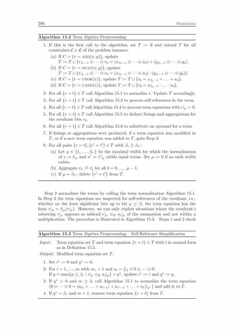
286 Presolving
Algorithm 15.2 Term Algebra Preprocessing
1. If this is the first call to the algorithm, set T := ∅ and extend T for allconstraints C ∈ C of the problem instance:
(a) If C = {r = add(x, y)}, updateT := T ∪ {rβr−1 ⊗ · · · ⊗ r0 = (xβr−1 ⊗ · · · ⊗ x0) + (yβr−1 ⊗ · · · ⊗ y0).
(b) If C = {r = mult(x, y)}, updateT := T ∪ {rβr−1 ⊗ · · · ⊗ r0 = (xβr−1 ⊗ · · · ⊗ x0) · (yβr−1 ⊗ · · · ⊗ y0)}.
(c) If C = {r = uxor(x)}, update T := T ∪ {r0 = xβx−1 + . . . + x0}.
(d) If C = {r = uand(x)}, update T := T ∪ {r0 = xβx−1 · . . . · x0}.
2. For all {r = t} ∈ T call Algorithm 15.1 to normalize t. Update T accordingly.
3. For all {r = t} ∈ T call Algorithm 15.3 to process self-references in the term.
4. For all {r = t} ∈ T call Algorithm 15.4 to process term equations with r|µ = 0.
5. For all {r = t} ∈ T call Algorithm 15.5 to deduce fixings and aggregations forthe resultant bits rb.
6. For all {r = t} ∈ T call Algorithm 15.6 to substitute an operand for a term.
7. If fixings or aggregations were produced, if a term equation was modified inT , or if a new term equation was added to T , goto Step 3.
8. For all pairs {r = t}, {r′ = t′} ∈ T with βr ≥ βr′ :
(a) Let µ ∈ {1, . . . , βr′} be the maximal width for which the normalizationof s := t|µ and s′ := t′|µ yields equal terms. Set µ := 0 if no such widthexists.
(b) Aggregate rb : ⋆= r′b for all b = 0, . . . , µ− 1.
(c) If µ = βr′ , delete {r′ = t′} from T .
Step 2 normalizes the terms by calling the term normalization Algorithm 15.1.In Step 3 the term equations are inspected for self-references of the resultant, i.e.,whether on the least significant bits up to bit µ ≤ βr the term equation has theform r|µ = t|µ(r|µ). However, we can only exploit situations where the resultant’ssubstring r|µ appears as addend r|µ ≡E ai|µ of the summation and not within amultiplication. The procedure is illustrated in Algorithm 15.3. Steps 1 and 2 check
Algorithm 15.3 Term Algebra Preprocessing – Self-Reference Simplification
Input : Term equation set T and term equation {r = t} ∈ T with t in normal formas in Definition 15.5.
Output : Modified term equation set T .
1. Set i⋆ := 0 and q⋆ := 0.
2. For i = 1, . . . ,m with mi = 1 and ai = fi1 ⊗ 0⊗ · · · ⊗ 0:If q = max{µ ≤ βr | r|µ ≡E ai|µ} > q⋆, update i⋆ := i and q⋆ := q.
3. If q⋆ > 0 and m ≥ 2, call Algorithm 15.1 to normalize the term equation{0⊗ · · · ⊗ 0 = (am + . . . + ai⋆+1 + ai⋆−1 + . . . + a1)|q⋆} and add it to T .
4. If q⋆ = βr and m = 1, remove term equation {r = t} from T .
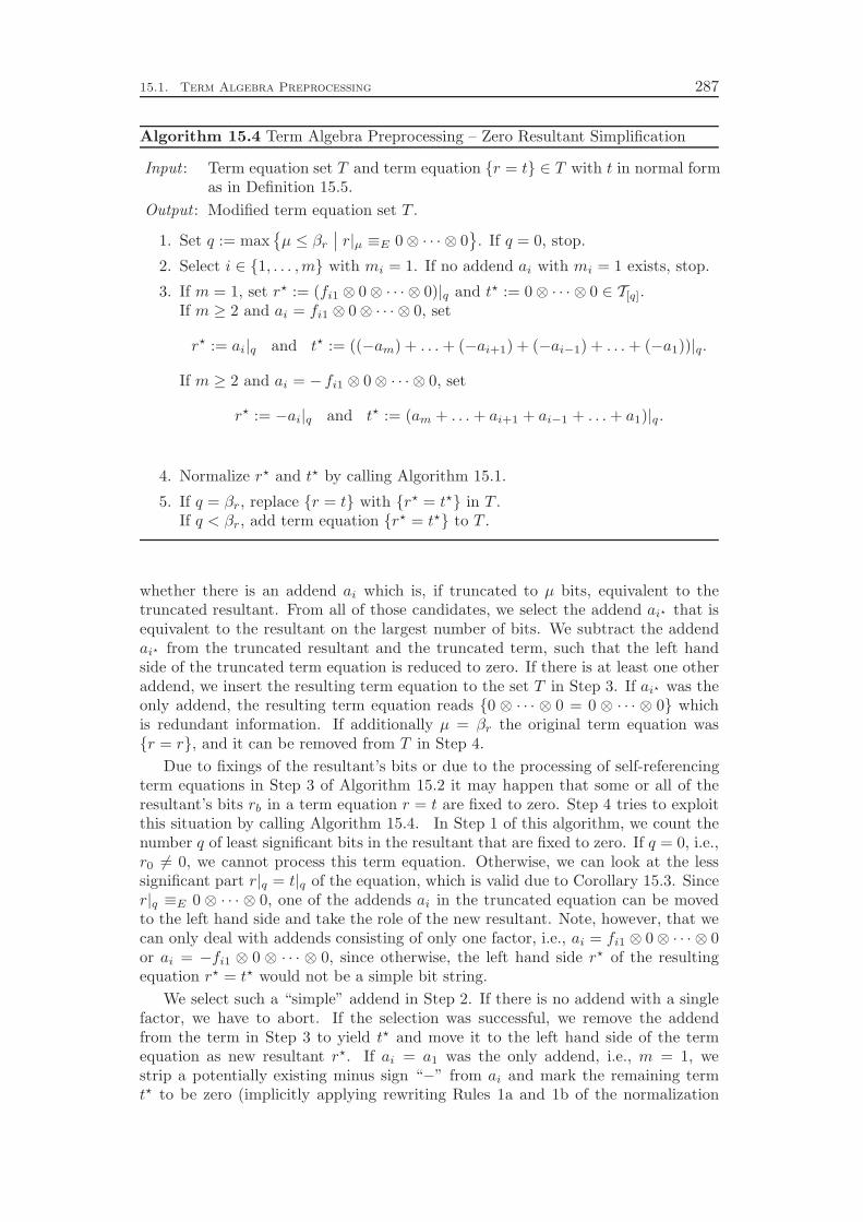
15.1. Term Algebra Preprocessing 287
Algorithm 15.4 Term Algebra Preprocessing – Zero Resultant Simplification
Input : Term equation set T and term equation {r = t} ∈ T with t in normal formas in Definition 15.5.
Output : Modified term equation set T .
1. Set q := max{µ ≤ βr
∣∣ r|µ ≡E 0⊗ · · · ⊗ 0
}. If q = 0, stop.
2. Select i ∈ {1, . . . ,m} with mi = 1. If no addend ai with mi = 1 exists, stop.
3. If m = 1, set r⋆ := (fi1 ⊗ 0⊗ · · · ⊗ 0)|q and t⋆ := 0⊗ · · · ⊗ 0 ∈ T[q].If m ≥ 2 and ai = fi1 ⊗ 0⊗ · · · ⊗ 0, set
r⋆ := ai|q and t⋆ := ((−am) + . . . + (−ai+1) + (−ai−1) + . . .+ (−a1))|q.
If m ≥ 2 and ai = − fi1 ⊗ 0⊗ · · · ⊗ 0, set
r⋆ := −ai|q and t⋆ := (am + . . . + ai+1 + ai−1 + . . . + a1)|q.
4. Normalize r⋆ and t⋆ by calling Algorithm 15.1.
5. If q = βr, replace {r = t} with {r⋆ = t⋆} in T .If q < βr, add term equation {r⋆ = t⋆} to T .
whether there is an addend ai which is, if truncated to µ bits, equivalent to thetruncated resultant. From all of those candidates, we select the addend ai⋆ that isequivalent to the resultant on the largest number of bits. We subtract the addendai⋆ from the truncated resultant and the truncated term, such that the left handside of the truncated term equation is reduced to zero. If there is at least one otheraddend, we insert the resulting term equation to the set T in Step 3. If ai⋆ was theonly addend, the resulting term equation reads {0 ⊗ · · · ⊗ 0 = 0 ⊗ · · · ⊗ 0} whichis redundant information. If additionally µ = βr the original term equation was{r = r}, and it can be removed from T in Step 4.
Due to fixings of the resultant’s bits or due to the processing of self-referencingterm equations in Step 3 of Algorithm 15.2 it may happen that some or all of theresultant’s bits rb in a term equation r = t are fixed to zero. Step 4 tries to exploitthis situation by calling Algorithm 15.4. In Step 1 of this algorithm, we count thenumber q of least significant bits in the resultant that are fixed to zero. If q = 0, i.e.,r0 6= 0, we cannot process this term equation. Otherwise, we can look at the lesssignificant part r|q = t|q of the equation, which is valid due to Corollary 15.3. Sincer|q ≡E 0 ⊗ · · · ⊗ 0, one of the addends ai in the truncated equation can be movedto the left hand side and take the role of the new resultant. Note, however, that wecan only deal with addends consisting of only one factor, i.e., ai = fi1 ⊗ 0⊗ · · · ⊗ 0or ai = −fi1 ⊗ 0 ⊗ · · · ⊗ 0, since otherwise, the left hand side r⋆ of the resultingequation r⋆ = t⋆ would not be a simple bit string.
We select such a “simple” addend in Step 2. If there is no addend with a singlefactor, we have to abort. If the selection was successful, we remove the addendfrom the term in Step 3 to yield t⋆ and move it to the left hand side of the termequation as new resultant r⋆. If ai = a1 was the only addend, i.e., m = 1, westrip a potentially existing minus sign “−” from ai and mark the remaining termt⋆ to be zero (implicitly applying rewriting Rules 1a and 1b of the normalization
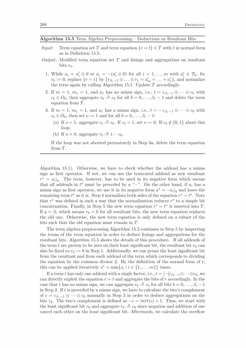
288 Presolving
Algorithm 15.5 Term Algebra Preprocessing – Deductions on Resultant Bits
Input : Term equation set T and term equation {r = t} ∈ T with t in normal formas in Definition 15.5.
Output : Modified term equation set T and fixings and aggregations on resultantbits rb.
1. While ai = a′i ⊗ 0 or ai = −(a′i ⊗ 0) for all i = 1, . . . ,m with a′i ∈ TΣ, fixr0 := 0, replace {r = t} by {rβr−1 ⊗ . . . ⊗ r1 = a′m + . . . + a′1}, and normalizethe term again by calling Algorithm 15.1. Update T accordingly.
2. If m = 1, m1 = 1, and a1 has no minus sign, i.e., t = cβr−1 ⊗ · · · ⊗ c0 withcb ∈ O0, then aggregate rb : ⋆= cb for all b = 0, . . . , βr − 1 and delete the termequation from T .
3. If m = 1, m1 = 1, and a1 has a minus sign, i.e., t = − cβr−1 ⊗ · · · ⊗ c0 withcb ∈ O0, then set o := 1 and for all b = 0, . . . , βr − 1:
(a) If o = 1, aggregate rb : ⋆= cb. If cb = 1, set o := 0. If cb /∈ {0, 1} abort thisloop.
(b) If o = 0, aggregate rb : ⋆= 1− cb.
If the loop was not aborted prematurely in Step 3a, delete the term equationfrom T .
Algorithm 15.1). Otherwise, we have to check whether the addend has a minussign as first operator. If not, we can use the truncated addend as new resultantr⋆ = ai|q. The term, however, has to be used in its negative form which meansthat all addends in t⋆ must be preceded by a “−”. On the other hand, if ai has aminus sign as first operator, we use it in its negative form a⋆ = −ai|q and leave theremaining term t⋆ as it is. Step 4 normalizes both sides of the equation r⋆ = t⋆. Notethat r⋆ was defined in such a way that the normalization reduces r⋆ to a simple bitconcatenation. Finally, in Step 5 the new term equation r⋆ = t⋆ is inserted into T .If q = βr which means rb = 0 for all resultant bits, the new term equation replacesthe old one. Otherwise, the new term equation is only defined on a subset of thebits such that the old equation must remain in T .
The term algebra preprocessing Algorithm 15.2 continues in Step 5 by inspectingthe terms of the term equation in order to deduce fixings and aggregations for theresultant bits. Algorithm 15.5 shows the details of this procedure. If all addends ofthe term t are proven to be zero on their least significant bit, the resultant bit r0 canalso be fixed to r0 := 0 in Step 1. Additionally, we can prune the least significant bitfrom the resultant and from each addend of the term which corresponds to dividingthe equation by the common divisor 2. By the definition of the normal form of t,this can be applied iteratively s⋆ = min{si | i ∈ {1, . . . ,m}} times.
If a term t has only one addend with a single factor, i.e., t = [−]cβr−1⊗· · ·⊗c0, wecan directly exploit the equation r = t and aggregate the bits of r accordingly. In thecase that t has no minus sign, we can aggregate rb : ⋆= cb for all bits b = 0, . . . , βr − 1in Step 2. If t is preceded by a minus sign, we have to calculate the two’s complementof c = cβr−1 ⊗ · · · ⊗ c0 manually in Step 3 in order to deduce aggregations on thebits rb. The two’s complement is defined as −c = not(c) + 1. Thus, we start withthe least significant bit r0 and aggregate r0 : ⋆= c0 since negation and addition of onecancel each other on the least significant bit. Afterwards, we calculate the overflow
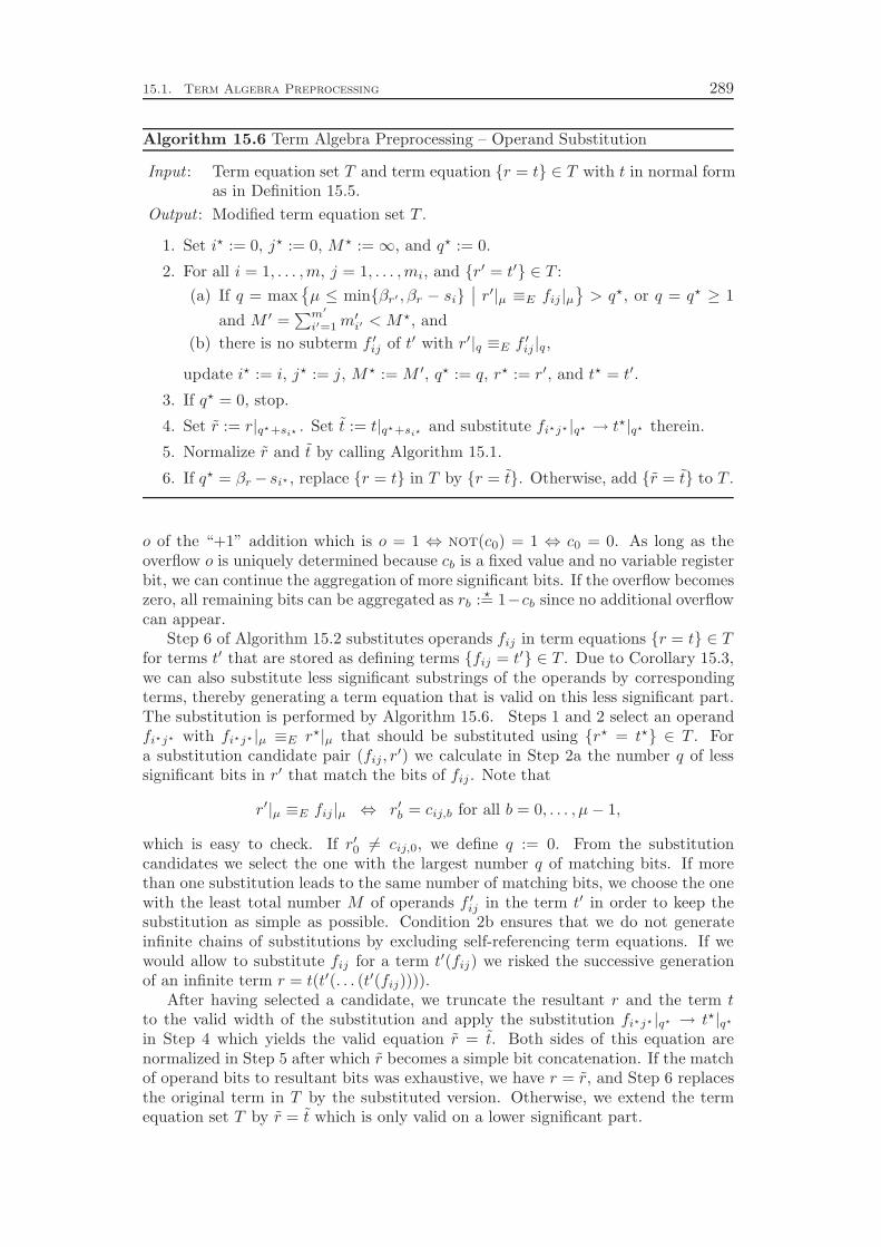
15.1. Term Algebra Preprocessing 289
Algorithm 15.6 Term Algebra Preprocessing – Operand Substitution
Input : Term equation set T and term equation {r = t} ∈ T with t in normal formas in Definition 15.5.
Output : Modified term equation set T .
1. Set i⋆ := 0, j⋆ := 0, M⋆ :=∞, and q⋆ := 0.
2. For all i = 1, . . . ,m, j = 1, . . . ,mi, and {r′ = t′} ∈ T :
(a) If q = max{µ ≤ min{βr′ , βr − si}
∣∣ r′|µ ≡E fij |µ
}> q⋆, or q = q⋆ ≥ 1
and M ′ =∑m′
i′=1m′i′ < M⋆, and
(b) there is no subterm f ′ij of t′ with r′|q ≡E f ′ij |q,
update i⋆ := i, j⋆ := j, M⋆ := M ′, q⋆ := q, r⋆ := r′, and t⋆ = t′.
3. If q⋆ = 0, stop.
4. Set r := r|q⋆+si⋆ . Set t := t|q⋆+si⋆ and substitute fi⋆j⋆ |q⋆ → t⋆|q⋆ therein.
5. Normalize r and t by calling Algorithm 15.1.
6. If q⋆ = βr− si⋆ , replace {r = t} in T by {r = t}. Otherwise, add {r = t} to T .
o of the “+1” addition which is o = 1 ⇔ not(c0) = 1 ⇔ c0 = 0. As long as theoverflow o is uniquely determined because cb is a fixed value and no variable registerbit, we can continue the aggregation of more significant bits. If the overflow becomeszero, all remaining bits can be aggregated as rb : ⋆= 1−cb since no additional overflowcan appear.
Step 6 of Algorithm 15.2 substitutes operands fij in term equations {r = t} ∈ Tfor terms t′ that are stored as defining terms {fij = t′} ∈ T . Due to Corollary 15.3,we can also substitute less significant substrings of the operands by correspondingterms, thereby generating a term equation that is valid on this less significant part.The substitution is performed by Algorithm 15.6. Steps 1 and 2 select an operandfi⋆j⋆ with fi⋆j⋆ |µ ≡E r⋆|µ that should be substituted using {r⋆ = t⋆} ∈ T . Fora substitution candidate pair (fij, r
′) we calculate in Step 2a the number q of lesssignificant bits in r′ that match the bits of fij . Note that
r′|µ ≡E fij |µ ⇔ r′b = cij,b for all b = 0, . . . , µ− 1,
which is easy to check. If r′0 6= cij,0, we define q := 0. From the substitutioncandidates we select the one with the largest number q of matching bits. If morethan one substitution leads to the same number of matching bits, we choose the onewith the least total number M of operands f ′ij in the term t′ in order to keep thesubstitution as simple as possible. Condition 2b ensures that we do not generateinfinite chains of substitutions by excluding self-referencing term equations. If wewould allow to substitute fij for a term t′(fij) we risked the successive generationof an infinite term r = t(t′(. . . (t′(fij)))).
After having selected a candidate, we truncate the resultant r and the term tto the valid width of the substitution and apply the substitution fi⋆j⋆ |q⋆ → t⋆|q⋆
in Step 4 which yields the valid equation r = t. Both sides of this equation arenormalized in Step 5 after which r becomes a simple bit concatenation. If the matchof operand bits to resultant bits was exhaustive, we have r = r, and Step 6 replacesthe original term in T by the substituted version. Otherwise, we extend the termequation set T by r = t which is only valid on a lower significant part.
290 Presolving
Steps 3 to 6 of the term algebra preprocessing Algorithm 15.2 are called itera-tively until no more problem reductions or term substitutions were applied. After-wards we inspect the final term equation database T in Step 8 to find pairs of termequations r = t and r′ = t′ for which the terms t and t′ are equivalent at least ona subset of the bits. Step 8a calculates the maximal width µ up to which the twoterms are equivalent. In Step 8b the corresponding resultant bits are aggregated. Ifall bits up to the full width βr′ of the shorter or equal resultant r′ were aggregated,the term equation r′ = t′ can be deleted from T in Step 8c.
Remark 15.8. Due to the fixings and aggregations of register bits jb and dueto the constraint rewritings performed in other presolving algorithms, our termrewriting system is not restricted to add, mult, and, or, xor, uand, uor, anduxor constraints. Instead, we also implicitly consider most of the other circuitoperators, namely minus, sub, not, zeroext, signext, and concat, as well asshl, shr, slice, read, and write if the offset operand is fixed.
In the current version of our code, we do not exploit the distributivity law, andwe do not mix addition and multiplication constraints in the substitution step. Weexpect that further preprocessing improvements can be achieved by incorporatingother constraints like eq, lt, ite or the subword access operators with variable offsetoperand into the term algebra and by exploiting rewriting rules like the distributivitylaw which link different operations.
15.2 Irrelevance Detection
In order to prove the validity of a given property, often only a part of the circuit hasto be considered. For example, if a property on an arithmetical logical unit (ALU)describes a certain aspect of the addition operation, the other operations of theALU are irrelevant. Suppose that ite constraints select the operation of the ALUby routing the output of the desired operation to the output register of the circuit,compare Figure 14.8 of Section 14.15 on page 252. The calculated values of the otheroperations are linked to the discarded inputs of the ite constraints and thereby donot contribute to the output of the circuit. These irrelevant constraints and theinvolved intermediate registers have no influence on the validity of the property andcan therefore be removed from the problem instance.
The detection of irrelevant parts of the circuit can also be applied to the localsubproblems during the branch-and-bound search. In particular, irrelevant registervariables need not to be considered as branching candidates. Disregarding locallyirrelevant variables in the branching decision can be seen as replacement for the moreindirect method of selecting the next branching variable under the literals involvedin the recent conflict clauses, which is employed in state-of-the-art SAT solvers [100].
The identification and removal of irrelevant parts of the circuit is also known aslocalization reduction which was developed by Kurshan [137] or cone of influencereduction, which is explained, for example, in Biere et al. [43] and Clarke et al. [61].Similar ideas can be found in the program slicing technique of Weiser [210, 211]for decomposing software systems. However, these techniques are employed for SATbased property checking only in presolving and not during the traversal of the searchtree. Current state-of-the-art SAT solvers rely on a very fast processing of the indi-vidual subproblems, spending most of the time for Boolean constraint propagation.Incorporating local cone of influence reduction would lead to a large increase in the
15.2. Irrelevance Detection 291
subproblem processing time. Thus, the performance of SAT solvers would mostlikely deteriorate. In contrast, our constraint integer programming solver spendsmuch more time on each individual subproblem with the hope that this will becompensated by a much smaller search tree. The additional overhead to furtherprune locally irrelevant parts of the circuit is negligible, in particular compared tothe time needed to solve the LP relaxations and to execute the domain propagationalgorithms.
We implemented the irrelevance detection as part of the domain propagation andpresolving algorithms of the circuit constraint handlers, see Chapter 14. The basicreasoning is as follows: whenever a register j is only used in a single constraintCi, and for all values of the other registers involved in Ci there exists a value forj such that the constraint is feasible, we can delete Ci from the problem. If acounter-example for the property is found, we can calculate a valid value for j ina postprocessing stage. Because all circuit operations are totally defined, we canin particular delete constraints for which the resultant r is not used in any otherconstraint. For certain operators, however, irrelevance detection can also be appliedto input registers.
The irrelevance detection procedure is illustrated in Algorithm 15.7. In Step 1the function graph G = (V,A) is created. Recall that this is a directed bipartitegraph G = (V ∪ VC, A) with two different types of nodes, namely register nodesV = {1, . . . , n} and constraint nodes VC = {C1, . . . , Cm}. The arc set is defined as
A = {(j , Ci) | register j is input of circuit operation Ci}
∪ {(Ci, j) | register j is output of circuit operation Ci}.
Note that although and and xor constraints are replaced in presolving by acorresponding number of unary uand and uxor constraints, they are still repre-sented as binary and and xor constraints in the function graph in order to preservethe structure of the graph. Additionally, whenever a constraint is deleted from theproblem because the register bits are fixed in a way such that the constraint willalways be feasible, its representative in the function graph is retained.
Constant registers in the property checking problem cannot be set to a matchingvalue while postprocessing a partial solution. Therefore, we have to make sure thatthey are not used to detect the irrelevance of a constraint. This is achieved by addingan extra node λ to the vertex set of G and linking it to the constant register verticesj in Step 2, thereby increasing their degree d(j) := d+(j) + d−(j).
Step 3 processes special situations in mult and ite constraints. If one of theinput registers of a mult constraint r = mult(x, y) is fixed to zero, the resultant rwill always be zero, independently from the value of the other operand. Therefore,we can unlink the other operand from the constraint vertex. If the selection operandx of an ite constraint r = ite(x, y, z) is fixed, the operand that is not selected by xdoes not contribute to the resultant. Again, it can be unlinked from the constraintvertex. If the two input registers y and z are equivalent, the resultant r will alsobe equal to this single value, independently from the selection operand x. Thus, wecan unlink x from the ite constraint.
Finally, in Step 4 we check for irrelevant constraints. If the degree d(r) of theresultant vertex of a constraint is equal to one, the resultant register is not usedin any other constraint and is detected by Condition 4a to be irrelevant for thevalidity of the property. We can delete the constraint and its resultant registerfrom the problem and calculate the register’s value in a postprocessing step if acounter-example has been found.
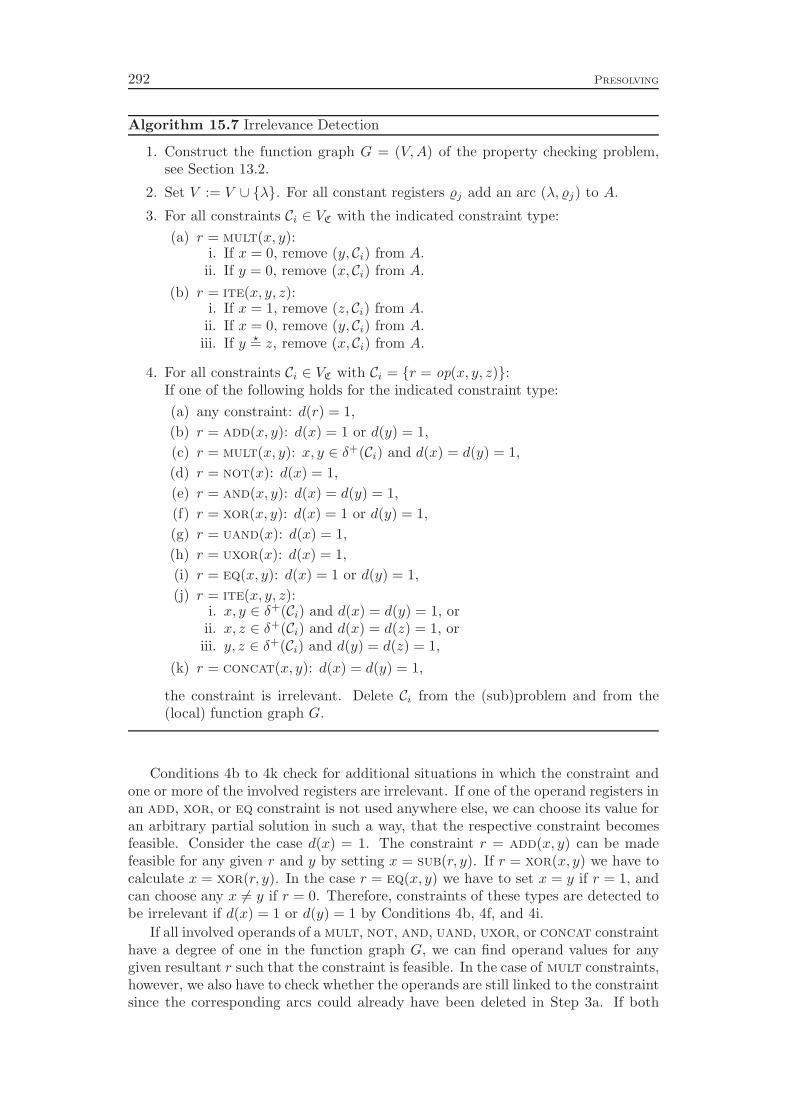
292 Presolving
Algorithm 15.7 Irrelevance Detection
1. Construct the function graph G = (V,A) of the property checking problem,see Section 13.2.
2. Set V := V ∪ {λ}. For all constant registers j add an arc (λ, j) to A.
3. For all constraints Ci ∈ VC with the indicated constraint type:
(a) r = mult(x, y):i. If x = 0, remove (y, Ci) from A.
ii. If y = 0, remove (x, Ci) from A.
(b) r = ite(x, y, z):i. If x = 1, remove (z, Ci) from A.
ii. If x = 0, remove (y, Ci) from A.iii. If y ⋆= z, remove (x, Ci) from A.
4. For all constraints Ci ∈ VC with Ci = {r = op(x, y, z)}:If one of the following holds for the indicated constraint type:
(a) any constraint: d(r) = 1,
(b) r = add(x, y): d(x) = 1 or d(y) = 1,
(c) r = mult(x, y): x, y ∈ δ+(Ci) and d(x) = d(y) = 1,
(d) r = not(x): d(x) = 1,
(e) r = and(x, y): d(x) = d(y) = 1,
(f) r = xor(x, y): d(x) = 1 or d(y) = 1,
(g) r = uand(x): d(x) = 1,
(h) r = uxor(x): d(x) = 1,
(i) r = eq(x, y): d(x) = 1 or d(y) = 1,
(j) r = ite(x, y, z):i. x, y ∈ δ+(Ci) and d(x) = d(y) = 1, or
ii. x, z ∈ δ+(Ci) and d(x) = d(z) = 1, oriii. y, z ∈ δ+(Ci) and d(y) = d(z) = 1,
(k) r = concat(x, y): d(x) = d(y) = 1,
the constraint is irrelevant. Delete Ci from the (sub)problem and from the(local) function graph G.
Conditions 4b to 4k check for additional situations in which the constraint andone or more of the involved registers are irrelevant. If one of the operand registers inan add, xor, or eq constraint is not used anywhere else, we can choose its value foran arbitrary partial solution in such a way, that the respective constraint becomesfeasible. Consider the case d(x) = 1. The constraint r = add(x, y) can be madefeasible for any given r and y by setting x = sub(r, y). If r = xor(x, y) we have tocalculate x = xor(r, y). In the case r = eq(x, y) we have to set x = y if r = 1, andcan choose any x 6= y if r = 0. Therefore, constraints of these types are detected tobe irrelevant if d(x) = 1 or d(y) = 1 by Conditions 4b, 4f, and 4i.
If all involved operands of a mult, not, and, uand, uxor, or concat constrainthave a degree of one in the function graph G, we can find operand values for anygiven resultant r such that the constraint is feasible. In the case of mult constraints,however, we also have to check whether the operands are still linked to the constraintsince the corresponding arcs could already have been deleted in Step 3a. If both
15.2. Irrelevance Detection 293
links still exist, we can always choose x = r and y = 1 to yield a valid constraintr = mult(x, y). Analogous postprocessings for a given resultant value r can beperformed for the other constraints:
⊲ x = not(r) for not constraints,
⊲ x = y = r for and constraints,
⊲ x = 0 if r = 0 and x = (1, . . . , 1) if r = 1 for uand constraints,
⊲ x = 0 if r = 0 and x = (0, . . . , 0, 1) if r = 1 for uxor constraints, and
⊲ x = (rβr−1, . . . , rβy) and y = (rβy−1, . . . , r0) for concat constraints.
For an ite constraint r = ite(x, y, z) we can detect irrelevance in the followingsituations. If the selection operand x and one of the case operands y or z haveboth a degree of one and are still linked to the constraint, irrelevance is detectedby Conditions 4(j)i or 4(j)ii, respectively. Assume d(x) = d(y) = 1. For a givenresultant value r and operand value z, we can always set x = 1 and y = r to turnr = ite(x, y, z) into a feasible constraint. On the other hand, if d(x) = d(z) = 1we just have to set x = 0 and z = r and do not have to care about the given valueof y. If neither of y and z is appearing in the remaining problem instance, i.e.,y, z ∈ δ+(Ci) and d(y) = d(z) = 1, we can postprocess y = z = r independently ofthe given value of x.

Chapter 16
Search
A branch-and-bound algorithm mainly consists of three steps that are iterated untilthe given problem instance has been solved, see Section 2.1:
1. Select a subproblem.
2. Process the subproblem.
3. If not pruned, split the subproblem into smaller parts.
The subproblem processing Step 2 for the property checking problem is covered inChapter 14. The current chapter explains the branching strategy for Step 3 and thenode selection rule for Step 1 that we employ.
16.1 Branching
The branching strategy in a branch-and-bound algorithm defines how the problemis recursively split into smaller subproblems, compare Section 2.1 and Chapter 5.Therefore, it is the most important component for determining the shape of thesearch tree. The ultimate goal of the branching strategy is to partition the probleminstance in such a way that it can be solved by processing only a minimal numberof subproblems. This global objective, however, is practically impossible to achieve.Instead, since we have to make our branching decision locally at each subproblem,we can at best try to follow some local criteria and hope that this yields a smallsearch tree for the global problem.
As mentioned in Section 2.1, the most popular branching strategy is to branchon variables, i.e., split the domain of a single variable into two parts. Since inbranch-and-bound solvers the domains of the variables are usually treated implic-itly, branching on variables has the advantage that one does not have to explicitlyadd constraints to the subproblems, thereby avoiding overhead in the subproblemmanagement. In particular, this is true for mixed integer programming and forSAT solving. For the same reason, we also apply branching on variables to theconstraint integer programming model of the property checking problem.
In mixed integer programming, the branching selection is mostly guided by theLP relaxation. Branching takes place on integer variables that have a fractionalvalue in the current LP solution. The idea is that the LP relaxation is undecidedabout these variables and we have to help the LP by forcing a decision. Indeed, onecan very often either find an integral LP solution after only a very few (comparedto the number of integer variables) branching steps or drive the LP relaxation toinfeasibility. Since we also have an LP relaxation at hand for the property checkingCIP, we adopt this idea and branch on integer variables with fractional LP solutionvalue. In contrast to mixed integer programming, an integral LP solution is notnecessarily a feasible CIP solution for the property checking problem, because notall circuit operators are linearized. Therefore, if the LP solution is integral but still
295
296 Search
not feasible, we have to branch on an integer variable with integral LP solutionvalue.
We saw in Chapter 5 that for mixed integer programming the change in theobjective value of the LP relaxation is a good indicator for selecting the branchingvariable. The full strong branching strategy yields very good results in the num-ber of branching nodes needed to solve the problem instances. In this strategy, weevaluate the impact of a potential branching decision by solving the two correspond-ing branching LPs. This is performed for every integer variable with fractional LPvalue. Then, we choose the variable for which the objective value of the branchingLPs increased the most. Unfortunately, full strong branching is very expensive suchthat the reduction in the number of branching nodes is usually outweighed by thetime needed to choose the branching variables. Therefore, one tries to approximatefull strong branching by less expensive methods, for example by estimating the LPobjective increase instead of calculating it by solving the branching LPs.
In contrast to most mixed integer programs, the property checking problem doesnot contain an objective function. As we model the problem as constraint integerprogram, we have to specify objective function coefficients for the variables, butthese are just artificial values. Therefore, it seems unlikely that the increase in theobjective value of the LP relaxations gives meaningful hints about the quality of thebranching candidates.
The satisfiability problem does not contain an objective function either. Cur-rent SAT solvers usually select the branching variable by some variant of the vari-able state independent decaying sum (VSIDS) strategy, see Moskewicz et al. [168].
This branching rule basically prefers variables that appear in the recently gener-ated conflict clauses. Goldberg and Novikov [100] improved this scheme in theirsolver BerkMin by noting that not only the variables in the final conflict clausesshould be regarded as promising branching candidates but also all other variablesinvolved in the conflicts, i.e., all variables on the conflict side of the conflict graphs,see Chapter 11.
In our property checking solver, we use a mixture of MIP and SAT branchingstrategies. Like in MIP, we select the branching variable under all integer variableswith fractional LP values. If the LP solution is integral but still not feasible for theCIP, we consider all unfixed integer variables (i.e., integer variables with at least twovalues in their current domain) as branching candidates. From these candidates wechoose the branching variable in a SAT-like manner by applying the VSIDS strategyof BerkMin. Additionally, we exploit our knowledge about the structure of thecircuit by disregarding variables that belong to registers which are irrelevant forthe current subproblem. Such registers are identified by the irrelevance detectiondescribed in Section 15.2.
16.2 Node Selection
The node selection strategy in a branch-and-bound solver determines in which orderthe nodes of the search tree, defined by the branching rule, are traversed. In mixedinteger programming one usually employs a mixture of best first and depth firstsearch, see Chapter 6. Best first search aims to improve the global dual bound asfast as possible by always selecting the subproblem with the lowest dual bound asnext subproblem to be processed. In fact, for a fixed branching strategy, a purebest first search traversal of the tree would solve the problem instance with the
16.2. Node Selection 297
minimal number of branching nodes. The disadvantage of best first search is thatit entails a large amount of switching between subproblems that are very far awayfrom each other in the search tree. This involves significant subproblem managementoverhead. Therefore, the best first search strategy is supplemented with depth firstsearch elements: after a best subproblem was selected, the search continues with afew iterations of depth first search, after which again a best subproblem is selected.
Since SAT does not contain an objective function, best first search does notmake sense for SAT. Indeed, state-of-the-art SAT solvers employ pure depth firstsearch. This has several advantages in the context of SAT. First, the subproblemmanagement is reduced to a minimum. In fact, SAT solvers completely avoid theexplicit generation of the search tree. Instead, they only keep track of the path tothe current subproblem and process the tree implicitly by using backtracking andby generating conflict clauses, see Chapter 11. The second advantage is that themanagement of conflict clauses is much easier. Most conflict clauses are only usefulin a certain part of the search tree, namely in the close vicinity of the node forwhich they were generated. Since depth first search completely solves the nodes inthis part of the tree before moving on to other regions, one can effectively identifyconflict clauses that are no longer useful and delete them from the clause database,see Goldberg and Novikov [100] for details. Nevertheless, depth first search entailsthe risk of getting stuck in an infeasible region of the search tree while there arelots of easy to find feasible solutions in other parts of the tree. To avoid such asituation, SAT solvers perform frequent restarts, which means to completely undoall branching decisions and start the search from scratch. Since conflict clauses areretained, the information gathered during the search is preserved.
Like the satisfiability problem, the property checking problem does not containan objective function. Therefore, we mainly employ depth first search. The problemof getting stuck in infeasible or fruitless parts of the tree, however, cannot be resolvedby restarts as easily as in SAT solvers. Because the effort in solving the LPs wouldbe lost, restarts were too costly. Therefore, we enrich the depth first search strategyby a small amount of best first search: after every 100 nodes of depth first search, weselect a best node from the tree and continue depth first search from this node. Thesubproblem management overhead for this combined strategy is marginal, the effectis similar to the restarts of SAT solvers, but the LP relaxations of the processednodes do not have to be solved again. A disadvantage compared to actual restartsis that we cannot undo our branching decisions.

Chapter 17
Computational Results
In this chapter we examine the computational effectiveness of the described con-straint integer programming techniques on industrial benchmarks obtained from ver-ification projects conducted by OneSpin Solutions. The instances are describedin Appendix A.4.
In a first series of benchmarks, we compare the CIP approach with the currentstate-of-the-art technology, which is to apply a SAT solver to the gate level represen-tation of the circuit and property. Before the SAT solver is called, a preprocessingstep is executed to simplify the instance at the gate level, which is based on binarydecision diagrams (BDDs). We use MiniSat 2.0 [82] to solve the resulting SAT in-stances. We also tried MiniSat 1.14, Siege v4 [196], and zChaff 2004.11.15 [168],but MiniSat 2.0 turned out to perform best on most of the instances of our test set.
A second set of benchmarks evaluates the impact of the problem specific presolv-ing methods that we described in Chapter 15, of probing as explained in Section 10.6,and of conflict analysis, which is described in Chapter 11. We also performed ad-ditional benchmark tests to assess the performance impact of other components likethe branching and node selection strategies, or the specification of the objectivefunction, but the alternative settings that we tried did not have a strong influenceon the performance.
17.1 Comparison of CIP and SAT
Tables 17.1 and 17.2 present the comparison of MiniSat and the CIP approach onan arithmetical logical unit (ALU). This circuit is able to perform add, sub, shl,shr, and signed and unsigned mult operations on two input registers. We considermultiple versions of the circuit which differ in the width of the input registers. Thewidth is depicted in the second column of the tables. Apart from the number ofbranching nodes and the time in CPU seconds needed to solve each instance, theother entries of the tables show the number of clauses and variables of the SATrepresentations in conjunctive normal form (CNF) and the number of constraintsand variables of the CIP instances. Note that the registers in the CIP formulationare represented as words and bits which are linked via special constraints, see Sec-tion 14.1. Thus, each register in the register transfer level description gives rise toone additional constraint, and the number of variables shown in the tables equalsthe total number of bits in the registers plus the number of 16-bit words that coverthe registers.
Overall, we investigated 11 different properties of the ALU circuit. Six of themturned out to be trivial for both, the SAT and the CIP solver, and they are notlisted in the tables. From the remaining five properties, two are invalid and threeare valid.
The results on the invalid properties are shown in Table 17.1. Recall that forsuch instances the task is to find a feasible solution, i.e., a counter-example to the
299
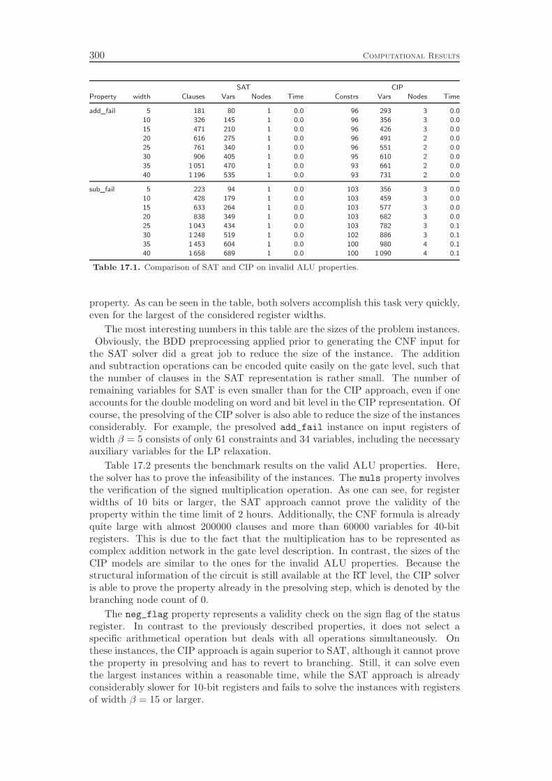
300 Computational Results
SAT CIP
Property width Clauses Vars Nodes Time Constrs Vars Nodes Time
add_fail 5 181 80 1 0.0 96 293 3 0.0
10 326 145 1 0.0 96 356 3 0.0
15 471 210 1 0.0 96 426 3 0.0
20 616 275 1 0.0 96 491 2 0.0
25 761 340 1 0.0 96 551 2 0.0
30 906 405 1 0.0 95 610 2 0.0
35 1 051 470 1 0.0 93 661 2 0.0
40 1 196 535 1 0.0 93 731 2 0.0
sub_fail 5 223 94 1 0.0 103 356 3 0.0
10 428 179 1 0.0 103 459 3 0.0
15 633 264 1 0.0 103 577 3 0.0
20 838 349 1 0.0 103 682 3 0.0
25 1 043 434 1 0.0 103 782 3 0.1
30 1 248 519 1 0.0 102 886 3 0.1
35 1 453 604 1 0.0 100 980 4 0.1
40 1 658 689 1 0.0 100 1 090 4 0.1
Table 17.1. Comparison of SAT and CIP on invalid ALU properties.
property. As can be seen in the table, both solvers accomplish this task very quickly,even for the largest of the considered register widths.
The most interesting numbers in this table are the sizes of the problem instances.Obviously, the BDD preprocessing applied prior to generating the CNF input for
the SAT solver did a great job to reduce the size of the instance. The additionand subtraction operations can be encoded quite easily on the gate level, such thatthe number of clauses in the SAT representation is rather small. The number ofremaining variables for SAT is even smaller than for the CIP approach, even if oneaccounts for the double modeling on word and bit level in the CIP representation. Ofcourse, the presolving of the CIP solver is also able to reduce the size of the instancesconsiderably. For example, the presolved add_fail instance on input registers ofwidth β = 5 consists of only 61 constraints and 34 variables, including the necessaryauxiliary variables for the LP relaxation.
Table 17.2 presents the benchmark results on the valid ALU properties. Here,the solver has to prove the infeasibility of the instances. The muls property involvesthe verification of the signed multiplication operation. As one can see, for registerwidths of 10 bits or larger, the SAT approach cannot prove the validity of theproperty within the time limit of 2 hours. Additionally, the CNF formula is alreadyquite large with almost 200000 clauses and more than 60000 variables for 40-bitregisters. This is due to the fact that the multiplication has to be represented ascomplex addition network in the gate level description. In contrast, the sizes of theCIP models are similar to the ones for the invalid ALU properties. Because thestructural information of the circuit is still available at the RT level, the CIP solveris able to prove the property already in the presolving step, which is denoted by thebranching node count of 0.
The neg_flag property represents a validity check on the sign flag of the statusregister. In contrast to the previously described properties, it does not select aspecific arithmetical operation but deals with all operations simultaneously. Onthese instances, the CIP approach is again superior to SAT, although it cannot provethe property in presolving and has to revert to branching. Still, it can solve eventhe largest instances within a reasonable time, while the SAT approach is alreadyconsiderably slower for 10-bit registers and fails to solve the instances with registersof width β = 15 or larger.
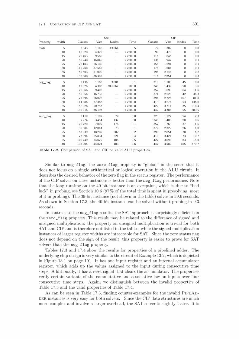
17.1. Comparison of CIP and SAT 301
SAT CIP
Property width Clauses Vars Nodes Time Constrs Vars Nodes Time
muls 5 3 343 1 140 13 864 0.5 79 302 0 0.0
10 12 828 4 325 — >7200.0 99 470 0 0.0
15 28 463 9 560 — >7200.0 116 646 0 0.0
20 50 248 16 845 — >7200.0 136 947 0 0.1
25 78 183 26 180 — >7200.0 156 1 294 0 0.1
30 112 268 37 565 — >7200.0 176 1 684 0 0.1
35 152 503 51 000 — >7200.0 196 2 144 0 0.2
40 198 888 66 485 — >7200.0 216 2 651 0 0.3
neg_flag 5 3 436 1 166 3 081 0.1 318 1 103 45 0.8
10 12 826 4 306 941 867 100.0 340 1 439 50 3.6
15 28 366 9 496 — >7200.0 352 1 693 64 11.6
20 50 056 16 736 — >7200.0 374 2 220 42 36.3
25 77 896 26 026 — >7200.0 394 2 726 107 81.8
30 111 886 37 366 — >7200.0 413 3 274 53 136.6
35 152 026 50 756 — >7200.0 422 3 714 35 218.4
40 198 316 66 196 — >7200.0 442 4 385 55 383.5
zero_flag 5 3 119 1 109 79 0.0 323 1 127 54 2.3
10 9 974 3 454 137 0.0 345 1 485 28 0.6
15 20 729 7 099 176 0.1 357 1 763 37 1.6
20 35 384 12 044 73 0.1 379 2 322 26 4.0
25 53 939 18 289 202 0.2 399 2 851 78 6.2
30 76 394 25 834 221 0.4 418 3 424 73 10.7
35 102 749 34 679 185 0.5 427 3 895 63 15.6
40 133 004 44 824 103 0.6 447 4 589 185 379.7
Table 17.2. Comparison of SAT and CIP on valid ALU properties.
Similar to neg_flag, the zero_flag property is “global” in the sense that itdoes not focus on a single arithmetical or logical operation in the ALU circuit. Itdescribes the desired behavior of the zero flag in the status register. The performanceof the CIP solver on these instances is better than the neg_flag performance. Notethat the long runtime on the 40-bit instance is an exception, which is due to “badluck” in probing, see Section 10.6 (97 % of the total time is spent in presolving, mostof it in probing). The 39-bit instance (not shown in the table) solves in 39.6 seconds.As shown in Section 17.3, the 40-bit instance can be solved without probing in 9.3seconds.
In contrast to the neg_flag results, the SAT approach is surprisingly efficient onthe zero_flag property. This result may be related to the difference of signed andunsigned multiplication: the property on unsigned multiplication is trivial for bothSAT and CIP and is therefore not listed in the tables, while the signed multiplicationinstances of larger register widths are intractable for SAT. Since the zero status flagdoes not depend on the sign of the result, this property is easier to prove for SATsolvers than the neg_flag property.
Tables 17.3 and 17.4 show the results for properties of a pipelined adder. Theunderlying chip design is very similar to the circuit of Example 13.2, which is depictedin Figure 13.1 on page 191. It has one input register and an internal accumulatorregister, which adds up the values assigned to the input during consecutive timesteps. Additionally, it has a reset signal that clears the accumulator. The propertiesverify certain variants of the commutative and associative law on inputs over fourconsecutive time steps. Again, we distinguish between the invalid properties ofTable 17.3 and the valid properties of Table 17.4.
As can be seen in Table 17.3, finding counter-examples for the invalid PipeAd-der instances is very easy for both solvers. Since the CIP data structures are muchmore complex and involve a larger overhead, the SAT solver is slightly faster. It is
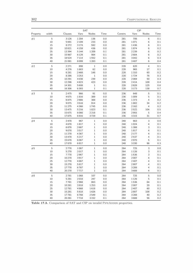
302 Computational Results
SAT CIP
Property width Clauses Vars Nodes Time Constrs Vars Nodes Time
#1 5 3 126 1 204 136 0.0 281 706 6 0.1
10 5 691 2 189 233 0.0 281 1 071 6 0.1
15 8 272 3 174 592 0.0 281 1 436 6 0.1
20 10 821 4 159 436 0.0 281 1 874 6 0.2
25 13 394 5 144 1 209 0.1 281 2 239 6 0.2
30 15 967 6 129 984 0.1 281 2 604 6 0.2
35 18 524 7 114 1 552 0.1 281 3 042 6 0.3
40 21 081 8 099 1 283 0.1 281 3 407 6 0.4
#2 5 2 271 898 1 0.0 228 620 4 0.1
10 4 276 1 683 62 0.0 228 965 17 0.1
15 6 281 2 468 148 0.0 228 1 310 60 0.2
20 8 286 3 253 1 0.0 228 1 724 76 0.3
25 10 291 4 038 239 0.0 228 2 069 50 0.3
30 12 296 4 823 423 0.0 228 2 414 109 0.4
35 14 301 5 608 1 0.1 228 2 828 125 0.6
40 16 306 6 393 1 0.1 228 3 173 138 0.7
#3 5 2 475 966 91 0.0 236 648 5 0.1
10 4 675 1 816 389 0.0 236 1 009 5 0.1
15 6 875 2 666 388 0.0 236 1 373 4 0.2
20 9 075 3 516 914 0.0 236 1 802 34 0.2
25 11 275 4 366 1 745 0.0 236 2 162 4 0.2
30 13 475 5 216 1 823 0.1 236 2 522 104 0.5
35 15 675 6 066 2 218 0.1 236 2 955 5 0.4
40 17 875 6 916 3 729 0.1 236 3 315 31 0.7
#4 5 2 478 967 1 0.0 248 663 3 0.0
10 4 678 1 817 1 0.0 248 1 024 4 0.1
15 6 878 2 667 1 0.0 248 1 388 3 0.1
20 9 078 3 517 1 0.0 248 1 817 4 0.1
25 11 278 4 367 1 0.0 248 2 177 4 0.1
30 13 478 5 217 1 0.0 248 2 537 4 0.1
35 15 678 6 067 1 0.0 248 2 970 5 0.1
40 17 878 6 917 1 0.0 248 3 330 96 0.3
#5 5 2 778 1 067 1 0.0 264 725 3 0.0
10 5 278 2 017 1 0.0 264 1 126 3 0.1
15 7 778 2 967 1 0.0 264 1 536 3 0.1
20 10 278 3 917 1 0.0 264 2 007 4 0.1
25 12 778 4 867 1 0.0 264 2 407 4 0.1
30 15 278 5 817 1 0.0 264 2 807 4 0.1
35 17 778 6 767 1 0.0 264 3 288 4 0.1
40 20 278 7 717 1 0.0 264 3 688 4 0.1
#8 5 2 781 1 068 107 0.0 264 725 5 0.0
10 5 281 2 018 247 0.0 264 1 126 5 0.1
15 7 781 2 968 863 0.0 264 1 536 64 0.1
20 10 281 3 918 1 253 0.0 264 2 007 20 0.1
25 12 781 4 868 1 618 0.0 264 2 407 60 0.2
30 15 281 5 818 1 626 0.0 264 2 807 108 0.2
35 17 781 6 768 2 549 0.1 264 3 288 40 0.2
40 20 281 7 718 3 152 0.1 264 3 688 56 0.2
Table 17.3. Comparison of SAT and CIP on invalid PipeAdder properties.
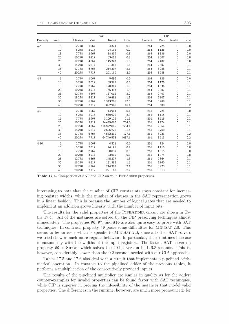
17.1. Comparison of CIP and SAT 303
SAT CIP
Property width Clauses Vars Nodes Time Constrs Vars Nodes Time
#6 5 2 778 1 067 4 321 0.0 264 725 0 0.0
10 5 278 2 017 24 195 0.2 264 1 126 0 0.0
15 7 778 2 967 58 839 0.5 264 1 536 0 0.0
20 10 278 3 917 83 615 0.8 264 2 007 0 0.0
25 12 778 4 867 145 377 1.3 264 2 407 0 0.0
30 15 278 5 817 191 388 1.6 264 2 807 0 0.1
35 17 778 6 767 214 307 2.1 264 3 288 0 0.1
40 20 278 7 717 291 160 2.9 264 3 688 0 0.1
#7 5 2 778 1 067 5 696 0.0 264 725 0 0.0
10 5 278 2 017 59 387 0.6 264 1 126 0 0.1
15 7 778 2 967 128 369 1.3 264 1 536 0 0.1
20 10 278 3 917 165 433 1.9 264 2 007 0 0.1
25 12 778 4 867 187 012 2.2 264 2 407 0 0.1
30 15 278 5 817 149 481 1.7 264 2 807 0 0.1
35 17 778 6 767 1 343 206 22.5 264 3 288 0 0.1
40 20 278 7 717 892 946 16.4 264 3 688 0 0.2
#9 5 2 778 1 067 14 901 0.1 261 724 0 0.0
10 5 278 2 017 630 929 8.9 261 1 115 0 0.1
15 7 778 2 967 1 109 126 21.3 261 1 515 0 0.1
20 10 278 3 917 24 485 660 764.0 261 1 974 0 0.1
25 12 778 4 867 119 922 885 5554.4 261 2 364 0 0.1
30 15 278 5 817 2 696 270 81.6 261 2 760 0 0.1
35 17 778 6 767 4 562 830 177.1 261 3 223 0 0.2
40 20 278 7 717 64 749 573 4087.1 261 3 613 0 0.2
#10 5 2 778 1 067 4 321 0.0 261 724 0 0.0
10 5 278 2 017 24 195 0.2 261 1 115 0 0.0
15 7 778 2 967 58 839 0.5 261 1 515 0 0.0
20 10 278 3 917 83 615 0.8 261 1 974 0 0.0
25 12 778 4 867 145 377 1.3 261 2 364 0 0.1
30 15 278 5 817 191 388 1.6 261 2 760 0 0.1
35 17 778 6 767 214 307 2.1 261 3 223 0 0.1
40 20 278 7 717 291 160 2.9 261 3 613 0 0.1
Table 17.4. Comparison of SAT and CIP on valid PipeAdder properties.
interesting to note that the number of CIP constraints stays constant for increas-ing register widths, while the number of clauses in the SAT representation growsin a linear fashion. This is because the number of logical gates that are needed toimplement an addition grows linearly with the number of input bits.
The results for the valid properties of the PipeAdder circuit are shown in Ta-ble 17.4. All of the instances are solved by the CIP presolving techniques almostimmediately. The properties #6, #7, and #10 are also quite easy to prove with SATtechniques. In contrast, property #9 poses some difficulties for MiniSat 2.0. Thisseems to be an issue which is specific to MiniSat 2.0, since all other SAT solverswe tried show a much more regular behavior. In particular, their runtimes increasemonotonously with the widths of the input registers. The fastest SAT solver onproperty #9 is Siege, which solves the 40-bit version in 146.8 seconds. This is,however, considerably slower than the 0.2 seconds needed with our CIP approach.
Tables 17.5 and 17.6 also deal with a circuit that implements a pipelined arith-metical operation. In contrast to the pipelined adder of the previous tables, itperforms a multiplication of the consecutively provided inputs.
The results of the pipelined multiplier are similar in quality as for the adder:counter-examples for invalid properties can be found faster with SAT techniques,while CIP is superior in proving the infeasibility of the instances that model validproperties. The differences in the runtime, however, are much more pronounced: for
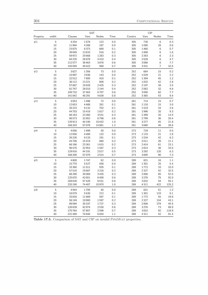
304 Computational Results
SAT CIP
Property width Clauses Vars Nodes Time Constrs Vars Nodes Time
#1 5 4 254 1 578 122 0.0 305 730 6 0.3
10 11 994 4 288 187 0.0 305 1 095 28 0.6
15 23 875 8 373 669 0.1 305 1 460 6 0.7
20 39 849 13 833 516 0.2 305 1 898 6 1.6
25 59 972 20 668 1 283 0.3 305 2 263 6 2.3
30 84 220 28 878 4 410 0.4 305 2 628 6 4.7
35 112 577 38 463 3 876 0.6 305 3 066 6 7.7
40 145 059 49 423 569 0.7 305 3 431 7 10.5
#2 5 3 627 1 356 73 0.0 252 664 15 0.2
10 10 997 3 936 143 0.0 252 1 029 21 2.2
15 22 512 7 895 418 0.1 252 1 394 45 1.2
20 38 112 13 221 808 0.2 252 1 832 42 2.8
25 57 867 19 928 2 425 0.3 252 2 197 39 3.5
30 81 747 28 010 2 144 0.4 252 2 562 32 4.6
35 109 732 37 463 6 707 0.6 252 3 000 82 7.7
40 141 842 48 291 4 639 0.8 252 3 365 43 9.4
#3 5 4 053 1 498 72 0.0 261 714 15 0.7
10 12 653 4 488 281 0.1 261 1 118 15 3.0
15 26 223 9 132 702 0.1 261 1 519 33 2.6
20 44 703 15 418 1 817 0.2 261 1 996 20 9.3
25 68 163 23 360 3 531 0.3 261 2 399 20 13.5
30 96 573 32 952 6 798 0.6 261 2 799 36 20.4
35 129 913 44 190 10 432 1.0 261 3 277 45 21.8
40 168 203 57 078 14 881 1.2 261 3 680 46 28.8
#4 5 4 056 1 499 50 0.0 273 729 11 0.5
10 12 656 4 489 132 0.0 273 1 133 21 2.8
15 26 226 9 133 191 0.1 273 1 534 42 6.2
20 44 706 15 419 880 0.2 273 2 011 28 11.1
25 68 166 23 361 1 615 0.2 273 2 414 61 23.1
30 96 576 32 953 1 587 0.3 273 2 814 38 33.0
35 129 916 44 191 2 517 0.5 273 3 292 120 6.3
40 168 206 57 079 2 514 0.7 273 3 695 90 7.3
#5 5 4 800 1 747 62 0.0 289 821 16 1.1
10 15 770 5 527 558 0.0 289 1 301 25 5.4
15 33 360 11 511 935 0.1 289 1 772 33 15.0
20 57 510 19 687 2 216 0.2 289 2 327 42 32.5
25 88 290 30 069 3 435 0.3 289 2 806 85 52.0
30 125 670 42 651 6 458 0.6 289 3 276 75 92.0
35 169 630 57 429 8 531 0.8 289 3 832 44 55.1
40 220 190 74 407 10 970 1.0 289 4 311 422 125.2
#8 5 4 944 1 795 40 0.0 289 821 51 1.2
10 16 079 5 630 212 0.1 289 1 301 133 8.1
15 33 834 11 669 587 0.1 289 1 772 55 19.8
20 58 149 19 900 1 597 0.2 289 2 327 154 43.1
25 89 094 30 337 1 727 0.3 289 2 806 279 45.5
30 126 639 42 974 2 530 0.6 289 3 276 73 89.9
35 170 764 57 807 2 596 0.7 289 3 832 92 118.9
40 221 489 74 840 6 834 1.1 289 4 311 42 91.4
Table 17.5. Comparison of SAT and CIP on invalid PipeMult properties.
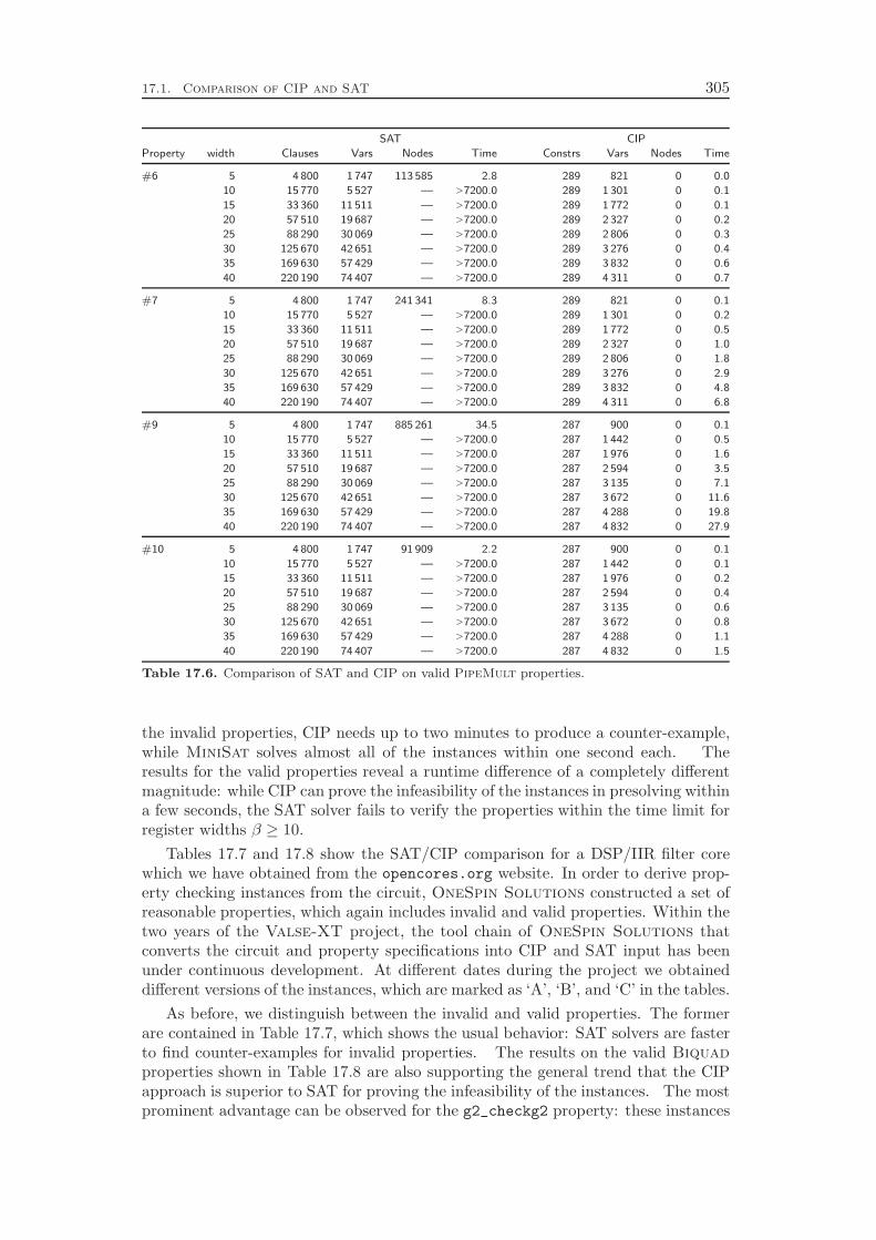
17.1. Comparison of CIP and SAT 305
SAT CIP
Property width Clauses Vars Nodes Time Constrs Vars Nodes Time
#6 5 4 800 1 747 113 585 2.8 289 821 0 0.0
10 15 770 5 527 — >7200.0 289 1 301 0 0.1
15 33 360 11 511 — >7200.0 289 1 772 0 0.1
20 57 510 19 687 — >7200.0 289 2 327 0 0.2
25 88 290 30 069 — >7200.0 289 2 806 0 0.3
30 125 670 42 651 — >7200.0 289 3 276 0 0.4
35 169 630 57 429 — >7200.0 289 3 832 0 0.6
40 220 190 74 407 — >7200.0 289 4 311 0 0.7
#7 5 4 800 1 747 241 341 8.3 289 821 0 0.1
10 15 770 5 527 — >7200.0 289 1 301 0 0.2
15 33 360 11 511 — >7200.0 289 1 772 0 0.5
20 57 510 19 687 — >7200.0 289 2 327 0 1.0
25 88 290 30 069 — >7200.0 289 2 806 0 1.8
30 125 670 42 651 — >7200.0 289 3 276 0 2.9
35 169 630 57 429 — >7200.0 289 3 832 0 4.8
40 220 190 74 407 — >7200.0 289 4 311 0 6.8
#9 5 4 800 1 747 885 261 34.5 287 900 0 0.1
10 15 770 5 527 — >7200.0 287 1 442 0 0.5
15 33 360 11 511 — >7200.0 287 1 976 0 1.6
20 57 510 19 687 — >7200.0 287 2 594 0 3.5
25 88 290 30 069 — >7200.0 287 3 135 0 7.1
30 125 670 42 651 — >7200.0 287 3 672 0 11.6
35 169 630 57 429 — >7200.0 287 4 288 0 19.8
40 220 190 74 407 — >7200.0 287 4 832 0 27.9
#10 5 4 800 1 747 91 909 2.2 287 900 0 0.1
10 15 770 5 527 — >7200.0 287 1 442 0 0.1
15 33 360 11 511 — >7200.0 287 1 976 0 0.2
20 57 510 19 687 — >7200.0 287 2 594 0 0.4
25 88 290 30 069 — >7200.0 287 3 135 0 0.6
30 125 670 42 651 — >7200.0 287 3 672 0 0.8
35 169 630 57 429 — >7200.0 287 4 288 0 1.1
40 220 190 74 407 — >7200.0 287 4 832 0 1.5
Table 17.6. Comparison of SAT and CIP on valid PipeMult properties.
the invalid properties, CIP needs up to two minutes to produce a counter-example,while MiniSat solves almost all of the instances within one second each. Theresults for the valid properties reveal a runtime difference of a completely differentmagnitude: while CIP can prove the infeasibility of the instances in presolving withina few seconds, the SAT solver fails to verify the properties within the time limit forregister widths β ≥ 10.
Tables 17.7 and 17.8 show the SAT/CIP comparison for a DSP/IIR filter corewhich we have obtained from the opencores.org website. In order to derive prop-erty checking instances from the circuit, OneSpin Solutions constructed a set ofreasonable properties, which again includes invalid and valid properties. Within thetwo years of the Valse-XT project, the tool chain of OneSpin Solutions thatconverts the circuit and property specifications into CIP and SAT input has beenunder continuous development. At different dates during the project we obtaineddifferent versions of the instances, which are marked as ‘A’, ‘B’, and ‘C’ in the tables.
As before, we distinguish between the invalid and valid properties. The formerare contained in Table 17.7, which shows the usual behavior: SAT solvers are fasterto find counter-examples for invalid properties. The results on the valid Biquadproperties shown in Table 17.8 are also supporting the general trend that the CIPapproach is superior to SAT for proving the infeasibility of the instances. The mostprominent advantage can be observed for the g2_checkg2 property: these instances
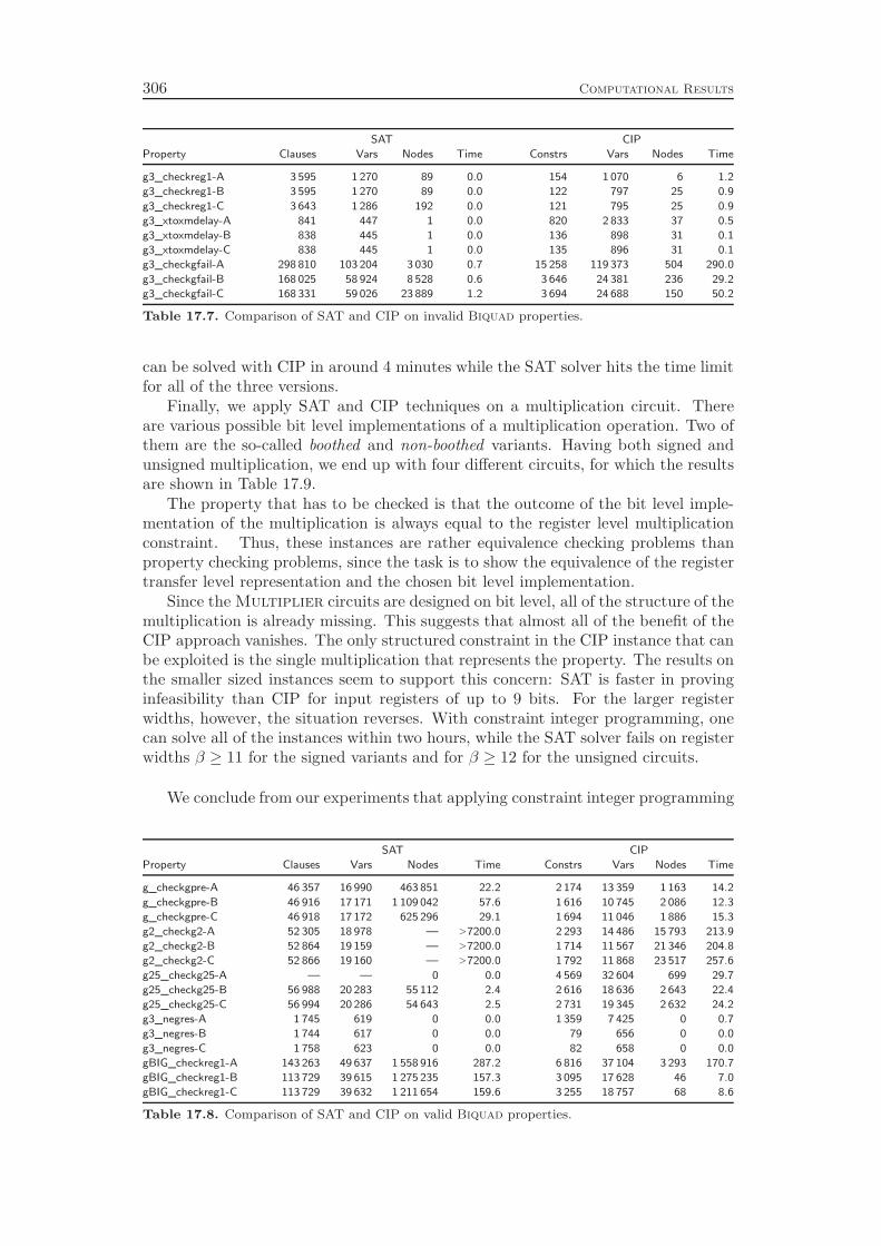
306 Computational Results
SAT CIP
Property Clauses Vars Nodes Time Constrs Vars Nodes Time
g3_checkreg1-A 3 595 1 270 89 0.0 154 1 070 6 1.2
g3_checkreg1-B 3 595 1 270 89 0.0 122 797 25 0.9
g3_checkreg1-C 3 643 1 286 192 0.0 121 795 25 0.9
g3_xtoxmdelay-A 841 447 1 0.0 820 2 833 37 0.5
g3_xtoxmdelay-B 838 445 1 0.0 136 898 31 0.1
g3_xtoxmdelay-C 838 445 1 0.0 135 896 31 0.1
g3_checkgfail-A 298 810 103 204 3 030 0.7 15 258 119 373 504 290.0
g3_checkgfail-B 168 025 58 924 8 528 0.6 3 646 24 381 236 29.2
g3_checkgfail-C 168 331 59 026 23 889 1.2 3 694 24 688 150 50.2
Table 17.7. Comparison of SAT and CIP on invalid Biquad properties.
can be solved with CIP in around 4 minutes while the SAT solver hits the time limitfor all of the three versions.
Finally, we apply SAT and CIP techniques on a multiplication circuit. Thereare various possible bit level implementations of a multiplication operation. Two ofthem are the so-called boothed and non-boothed variants. Having both signed andunsigned multiplication, we end up with four different circuits, for which the resultsare shown in Table 17.9.
The property that has to be checked is that the outcome of the bit level imple-mentation of the multiplication is always equal to the register level multiplicationconstraint. Thus, these instances are rather equivalence checking problems thanproperty checking problems, since the task is to show the equivalence of the registertransfer level representation and the chosen bit level implementation.
Since the Multiplier circuits are designed on bit level, all of the structure of themultiplication is already missing. This suggests that almost all of the benefit of theCIP approach vanishes. The only structured constraint in the CIP instance that canbe exploited is the single multiplication that represents the property. The results onthe smaller sized instances seem to support this concern: SAT is faster in provinginfeasibility than CIP for input registers of up to 9 bits. For the larger registerwidths, however, the situation reverses. With constraint integer programming, onecan solve all of the instances within two hours, while the SAT solver fails on registerwidths β ≥ 11 for the signed variants and for β ≥ 12 for the unsigned circuits.
We conclude from our experiments that applying constraint integer programming
SAT CIP
Property Clauses Vars Nodes Time Constrs Vars Nodes Time
g_checkgpre-A 46 357 16 990 463 851 22.2 2 174 13 359 1 163 14.2
g_checkgpre-B 46 916 17 171 1 109 042 57.6 1 616 10 745 2 086 12.3
g_checkgpre-C 46 918 17 172 625 296 29.1 1 694 11 046 1 886 15.3
g2_checkg2-A 52 305 18 978 — >7200.0 2 293 14 486 15 793 213.9
g2_checkg2-B 52 864 19 159 — >7200.0 1 714 11 567 21 346 204.8
g2_checkg2-C 52 866 19 160 — >7200.0 1 792 11 868 23 517 257.6
g25_checkg25-A — — 0 0.0 4 569 32 604 699 29.7
g25_checkg25-B 56 988 20 283 55 112 2.4 2 616 18 636 2 643 22.4
g25_checkg25-C 56 994 20 286 54 643 2.5 2 731 19 345 2 632 24.2
g3_negres-A 1 745 619 0 0.0 1 359 7 425 0 0.7
g3_negres-B 1 744 617 0 0.0 79 656 0 0.0
g3_negres-C 1 758 623 0 0.0 82 658 0 0.0
gBIG_checkreg1-A 143 263 49 637 1 558 916 287.2 6 816 37 104 3 293 170.7
gBIG_checkreg1-B 113 729 39 615 1 275 235 157.3 3 095 17 628 46 7.0
gBIG_checkreg1-C 113 729 39 632 1 211 654 159.6 3 255 18 757 68 8.6
Table 17.8. Comparison of SAT and CIP on valid Biquad properties.
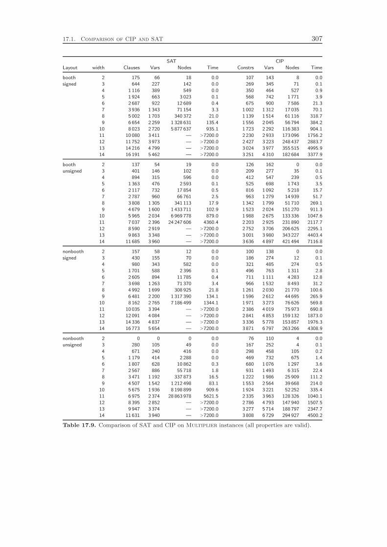
17.1. Comparison of CIP and SAT 307
SAT CIP
Layout width Clauses Vars Nodes Time Constrs Vars Nodes Time
booth 2 175 66 18 0.0 107 143 8 0.0
signed 3 644 227 142 0.0 269 345 71 0.1
4 1 116 389 549 0.0 350 464 527 0.9
5 1 924 663 3 023 0.1 568 742 1 771 3.9
6 2 687 922 12 689 0.4 675 900 7 586 21.3
7 3 936 1 343 71 154 3.3 1 002 1 312 17 035 70.1
8 5 002 1 703 340 372 21.0 1 139 1 514 61 116 318.7
9 6 654 2 259 1 328 631 135.4 1 556 2 045 56 794 384.2
10 8 023 2 720 5 877 637 935.1 1 723 2 292 116 383 904.1
11 10 080 3 411 — >7200.0 2 230 2 933 173 096 1756.2
12 11 752 3 973 — >7200.0 2 427 3 223 248 437 2883.7
13 14 216 4 799 — >7200.0 3 024 3 977 355 515 4995.9
14 16 191 5 462 — >7200.0 3 251 4 310 182 684 3377.9
booth 2 137 54 19 0.0 126 162 0 0.0
unsigned 3 401 146 102 0.0 209 277 35 0.1
4 894 315 596 0.0 412 547 239 0.5
5 1 363 476 2 593 0.1 525 698 1 743 3.5
6 2 117 732 17 854 0.5 816 1 092 5 218 15.7
7 2 787 960 66 761 2.5 963 1 279 14 939 51.7
8 3 808 1 305 341 113 17.9 1 342 1 799 51 710 269.1
9 4 679 1 600 1 433 711 102.9 1 523 2 024 151 270 911.3
10 5 965 2 034 6 969 778 879.0 1 988 2 675 133 336 1047.6
11 7 037 2 396 24 247 606 4360.4 2 203 2 925 231 890 2117.7
12 8 590 2 919 — >7200.0 2 752 3 706 206 625 2295.1
13 9 863 3 348 — >7200.0 3 001 3 980 343 227 4403.4
14 11 685 3 960 — >7200.0 3 636 4 897 421 494 7116.8
nonbooth 2 157 58 12 0.0 100 138 0 0.0
signed 3 430 155 70 0.0 186 274 12 0.1
4 980 343 582 0.0 321 485 274 0.5
5 1 701 588 2 396 0.1 496 763 1 311 2.8
6 2 605 894 11 785 0.4 711 1 111 4 283 12.8
7 3 698 1 263 71 370 3.4 966 1 532 8 493 31.2
8 4 992 1 699 308 925 21.8 1 261 2 030 21 770 100.6
9 6 481 2 200 1 317 390 134.1 1 596 2 612 44 695 265.9
10 8 162 2 765 7 186 499 1344.1 1 971 3 273 76 626 569.8
11 10 035 3 394 — >7200.0 2 386 4 019 75 973 690.8
12 12 091 4 084 — >7200.0 2 841 4 853 159 132 1873.0
13 14 336 4 837 — >7200.0 3 336 5 778 153 857 1976.3
14 16 773 5 654 — >7200.0 3 871 6 797 263 266 4308.9
nonbooth 2 0 0 0 0.0 76 110 4 0.0
unsigned 3 280 105 49 0.0 167 252 4 0.1
4 671 240 416 0.0 298 458 105 0.2
5 1 179 414 2 288 0.0 469 732 675 1.4
6 1 807 628 10 862 0.3 680 1 076 1 297 3.6
7 2 567 886 55 718 1.8 931 1 493 6 315 22.4
8 3 471 1 192 337 873 16.5 1 222 1 986 25 909 111.2
9 4 507 1 542 1 212 498 83.1 1 553 2 564 39 668 214.0
10 5 675 1 936 8 198 899 909.6 1 924 3 221 52 252 335.4
11 6 975 2 374 28 863 978 5621.5 2 335 3 963 128 326 1040.1
12 8 395 2 852 — >7200.0 2 786 4 793 147 940 1507.5
13 9 947 3 374 — >7200.0 3 277 5 714 188 797 2347.7
14 11 631 3 940 — >7200.0 3 808 6 729 294 927 4500.2
Table 17.9. Comparison of SAT and CIP on Multiplier instances (all properties are valid).
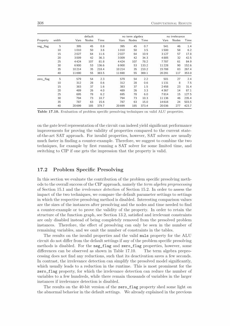
308 Computational Results
default no term algebra no irrelevance
Property width Vars Nodes Time Vars Nodes Time Vars Nodes Time
neg_flag 5 395 45 0.8 395 45 0.7 541 46 1.4
10 1 010 50 3.6 1 010 50 3.5 1 500 58 6.2
15 2 027 64 11.6 2 027 64 10.9 3 127 57 17.8
20 3 009 42 36.3 3 009 42 34.3 4 885 32 42.5
25 4 424 107 81.8 4 424 107 78.2 7 787 61 84.9
30 6 900 53 136.6 6 900 53 133.2 11 228 90 152.6
35 10 214 35 218.4 10 214 35 210.2 15 788 83 267.4
40 11 690 55 383.5 11 690 55 369.1 20 291 117 353.0
zero_flag 5 579 54 2.3 579 54 2.2 501 27 2.4
10 312 28 0.6 312 28 0.6 1 131 8 7.5
15 383 37 1.6 383 37 1.5 2 458 23 31.4
20 489 26 4.0 489 26 3.3 4 367 14 87.1
25 695 78 6.2 695 78 6.0 7 814 15 127.5
30 794 73 10.7 794 73 10.3 11 136 46 235.4
35 787 63 15.6 787 63 15.0 14 616 24 503.5
40 20 699 185 379.7 20 699 185 373.4 20 036 277 423.7
Table 17.10. Evaluation of problem specific presolving techniques on valid ALU properties.
on the gate level representation of the circuit can indeed yield significant performanceimprovements for proving the validity of properties compared to the current state-of-the-art SAT approach. For invalid properties, however, SAT solvers are usuallymuch faster in finding a counter-example. Therefore, we suggest to combine the twotechniques, for example by first running a SAT solver for some limited time, andswitching to CIP if one gets the impression that the property is valid.
17.2 Problem Specific Presolving
In this section we evaluate the contribution of the problem specific presolving meth-ods to the overall success of the CIP approach, namely the term algebra preprocessingof Section 15.1 and the irrelevance detection of Section 15.2. In order to assess theimpact of the two techniques, we compare the default parameter settings to settingsin which the respective presolving method is disabled. Interesting comparison valuesare the sizes of the instances after presolving and the nodes and time needed to finda counter-example or to prove the validity of the property. In order to retain thestructure of the function graph, see Section 13.2, satisfied and irrelevant constraintsare only disabled instead of being completely removed from the presolved probleminstances. Therefore, the effect of presolving can only be seen in the number ofremaining variables, and we omit the number of constraints in the tables.
The results on the invalid properties and the valid muls property for the ALUcircuit do not differ from the default settings if any of the problem specific presolvingmethods is disabled. For the neg_flag and zero_flag properties, however, somedifferences can be observed as shown in Table 17.10. The term algebra prepro-cessing does not find any reductions, such that its deactivation saves a few seconds.In contrast, the irrelevance detection can simplify the presolved model significantly,which usually leads to a reduction in the runtime. This is most prominent for thezero_flag property, for which the irrelevance detection can reduce the number ofvariables to a few hundreds, while there remain thousands of variables in the largerinstances if irrelevance detection is disabled.
The results on the 40-bit version of the zero_flag property shed some light onthe abnormal behavior in the default settings. We already explained in the previous
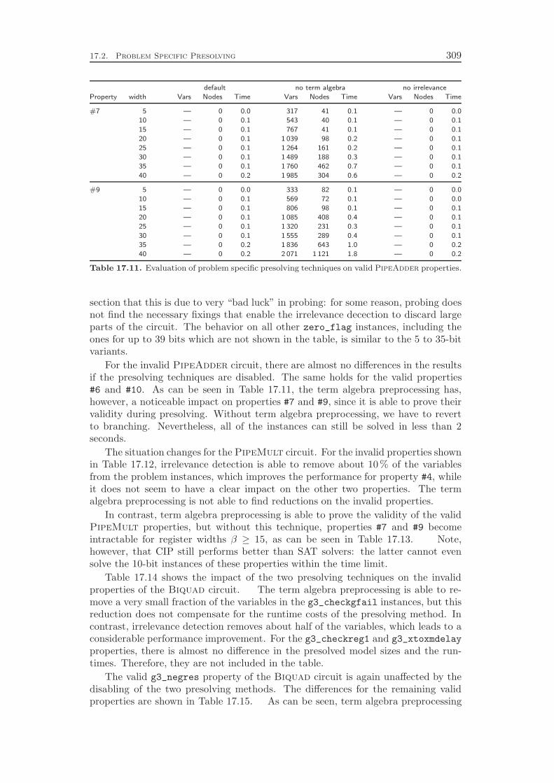
17.2. Problem Specific Presolving 309
default no term algebra no irrelevance
Property width Vars Nodes Time Vars Nodes Time Vars Nodes Time
#7 5 — 0 0.0 317 41 0.1 — 0 0.0
10 — 0 0.1 543 40 0.1 — 0 0.1
15 — 0 0.1 767 41 0.1 — 0 0.1
20 — 0 0.1 1 039 98 0.2 — 0 0.1
25 — 0 0.1 1 264 161 0.2 — 0 0.1
30 — 0 0.1 1 489 188 0.3 — 0 0.1
35 — 0 0.1 1 760 462 0.7 — 0 0.1
40 — 0 0.2 1 985 304 0.6 — 0 0.2
#9 5 — 0 0.0 333 82 0.1 — 0 0.0
10 — 0 0.1 569 72 0.1 — 0 0.0
15 — 0 0.1 806 98 0.1 — 0 0.1
20 — 0 0.1 1 085 408 0.4 — 0 0.1
25 — 0 0.1 1 320 231 0.3 — 0 0.1
30 — 0 0.1 1 555 289 0.4 — 0 0.1
35 — 0 0.2 1 836 643 1.0 — 0 0.2
40 — 0 0.2 2 071 1 121 1.8 — 0 0.2
Table 17.11. Evaluation of problem specific presolving techniques on valid PipeAdder properties.
section that this is due to very “bad luck” in probing: for some reason, probing doesnot find the necessary fixings that enable the irrelevance decection to discard largeparts of the circuit. The behavior on all other zero_flag instances, including theones for up to 39 bits which are not shown in the table, is similar to the 5 to 35-bitvariants.
For the invalid PipeAdder circuit, there are almost no differences in the resultsif the presolving techniques are disabled. The same holds for the valid properties#6 and #10. As can be seen in Table 17.11, the term algebra preprocessing has,however, a noticeable impact on properties #7 and #9, since it is able to prove theirvalidity during presolving. Without term algebra preprocessing, we have to revertto branching. Nevertheless, all of the instances can still be solved in less than 2seconds.
The situation changes for the PipeMult circuit. For the invalid properties shownin Table 17.12, irrelevance detection is able to remove about 10 % of the variablesfrom the problem instances, which improves the performance for property #4, whileit does not seem to have a clear impact on the other two properties. The termalgebra preprocessing is not able to find reductions on the invalid properties.
In contrast, term algebra preprocessing is able to prove the validity of the validPipeMult properties, but without this technique, properties #7 and #9 becomeintractable for register widths β ≥ 15, as can be seen in Table 17.13. Note,however, that CIP still performs better than SAT solvers: the latter cannot evensolve the 10-bit instances of these properties within the time limit.
Table 17.14 shows the impact of the two presolving techniques on the invalidproperties of the Biquad circuit. The term algebra preprocessing is able to re-move a very small fraction of the variables in the g3_checkgfail instances, but thisreduction does not compensate for the runtime costs of the presolving method. Incontrast, irrelevance detection removes about half of the variables, which leads to aconsiderable performance improvement. For the g3_checkreg1 and g3_xtoxmdelay
properties, there is almost no difference in the presolved model sizes and the run-times. Therefore, they are not included in the table.
The valid g3_negres property of the Biquad circuit is again unaffected by thedisabling of the two presolving methods. The differences for the remaining validproperties are shown in Table 17.15. As can be seen, term algebra preprocessing
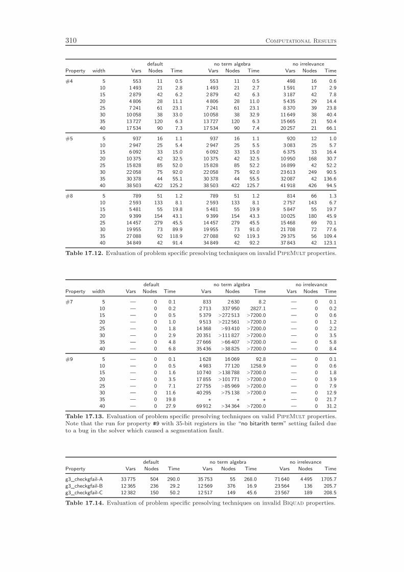
310 Computational Results
default no term algebra no irrelevance
Property width Vars Nodes Time Vars Nodes Time Vars Nodes Time
#4 5 553 11 0.5 553 11 0.5 498 16 0.6
10 1 493 21 2.8 1 493 21 2.7 1 591 17 2.9
15 2 879 42 6.2 2 879 42 6.3 3 187 42 7.8
20 4 806 28 11.1 4 806 28 11.0 5 435 29 14.4
25 7 241 61 23.1 7 241 61 23.1 8 370 39 23.8
30 10 058 38 33.0 10 058 38 32.9 11 649 38 40.4
35 13 727 120 6.3 13 727 120 6.3 15 665 21 50.4
40 17 534 90 7.3 17 534 90 7.4 20 257 21 66.1
#5 5 937 16 1.1 937 16 1.1 920 12 1.0
10 2 947 25 5.4 2 947 25 5.5 3 083 25 5.7
15 6 092 33 15.0 6 092 33 15.0 6 375 33 16.4
20 10 375 42 32.5 10 375 42 32.5 10 950 168 30.7
25 15 828 85 52.0 15 828 85 52.2 16 899 42 52.2
30 22 058 75 92.0 22 058 75 92.0 23 613 249 90.5
35 30 378 44 55.1 30 378 44 55.5 32 087 42 136.6
40 38 503 422 125.2 38 503 422 125.7 41 918 426 94.5
#8 5 789 51 1.2 789 51 1.2 814 66 1.3
10 2 593 133 8.1 2 593 133 8.1 2 757 143 6.7
15 5 481 55 19.8 5 481 55 19.9 5 847 55 19.7
20 9 399 154 43.1 9 399 154 43.3 10 025 180 45.9
25 14 457 279 45.5 14 457 279 45.5 15 468 69 70.1
30 19 955 73 89.9 19 955 73 91.0 21 708 72 77.6
35 27 088 92 118.9 27 088 92 119.3 29 375 56 109.4
40 34 849 42 91.4 34 849 42 92.2 37 843 42 123.1
Table 17.12. Evaluation of problem specific presolving techniques on invalid PipeMult properties.
default no term algebra no irrelevance
Property width Vars Nodes Time Vars Nodes Time Vars Nodes Time
#7 5 — 0 0.1 833 2 630 8.2 — 0 0.1
10 — 0 0.2 2 713 337 950 2827.1 — 0 0.2
15 — 0 0.5 5 379 >272 513 >7200.0 — 0 0.6
20 — 0 1.0 9 513 >212 561 >7200.0 — 0 1.2
25 — 0 1.8 14 368 >93 410 >7200.0 — 0 2.2
30 — 0 2.9 20 351 >111 827 >7200.0 — 0 3.5
35 — 0 4.8 27 666 >66 407 >7200.0 — 0 5.8
40 — 0 6.8 35 436 >38 825 >7200.0 — 0 8.4
#9 5 — 0 0.1 1 628 16 069 92.8 — 0 0.1
10 — 0 0.5 4 983 77 120 1258.9 — 0 0.6
15 — 0 1.6 10 740 >138 788 >7200.0 — 0 1.8
20 — 0 3.5 17 855 >101 771 >7200.0 — 0 3.9
25 — 0 7.1 27 755 >85 969 >7200.0 — 0 7.9
30 — 0 11.6 40 295 >75 138 >7200.0 — 0 12.9
35 — 0 19.8 ⋆ ⋆ ⋆ — 0 21.7
40 — 0 27.9 69 912 >34 364 >7200.0 — 0 31.2
Table 17.13. Evaluation of problem specific presolving techniques on valid PipeMult properties.Note that the run for property #9 with 35-bit registers in the “no bitarith term” setting failed dueto a bug in the solver which caused a segmentation fault.
default no term algebra no irrelevance
Property Vars Nodes Time Vars Nodes Time Vars Nodes Time
g3_checkgfail-A 33 775 504 290.0 35 753 55 268.0 71 640 4 495 1705.7
g3_checkgfail-B 12 365 236 29.2 12 569 376 16.9 23 564 136 205.7
g3_checkgfail-C 12 382 150 50.2 12 517 149 45.6 23 567 189 208.5
Table 17.14. Evaluation of problem specific presolving techniques on invalid Biquad properties.
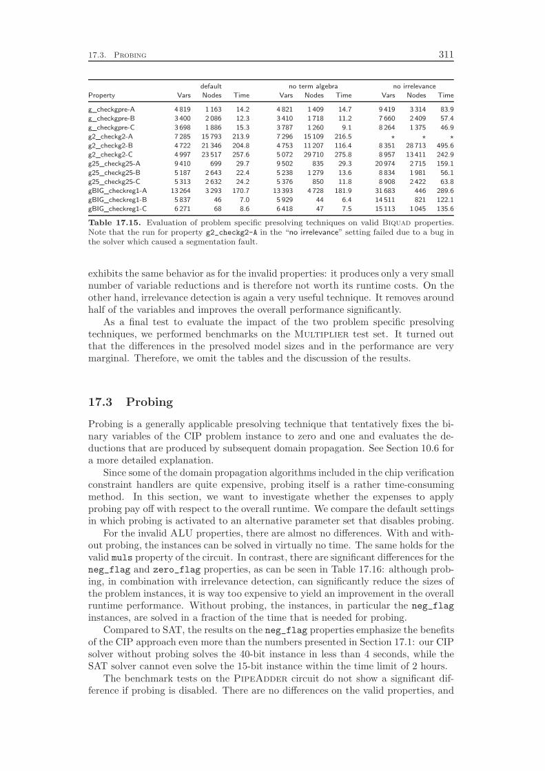
17.3. Probing 311
default no term algebra no irrelevance
Property Vars Nodes Time Vars Nodes Time Vars Nodes Time
g_checkgpre-A 4 819 1 163 14.2 4 821 1 409 14.7 9 419 3 314 83.9
g_checkgpre-B 3 400 2 086 12.3 3 410 1 718 11.2 7 660 2 409 57.4
g_checkgpre-C 3 698 1 886 15.3 3 787 1 260 9.1 8 264 1 375 46.9
g2_checkg2-A 7 285 15 793 213.9 7 296 15 109 216.5 ⋆ ⋆ ⋆
g2_checkg2-B 4 722 21 346 204.8 4 753 11 207 116.4 8 351 28 713 495.6
g2_checkg2-C 4 997 23 517 257.6 5 072 29 710 275.8 8 957 13 411 242.9
g25_checkg25-A 9 410 699 29.7 9 502 835 29.3 20 974 2 715 159.1
g25_checkg25-B 5 187 2 643 22.4 5 238 1 279 13.6 8 834 1 981 56.1
g25_checkg25-C 5 313 2 632 24.2 5 376 850 11.8 8 908 2 422 63.8
gBIG_checkreg1-A 13 264 3 293 170.7 13 393 4 728 181.9 31 683 446 289.6
gBIG_checkreg1-B 5 837 46 7.0 5 929 44 6.4 14 511 821 122.1
gBIG_checkreg1-C 6 271 68 8.6 6 418 47 7.5 15 113 1 045 135.6
Table 17.15. Evaluation of problem specific presolving techniques on valid Biquad properties.Note that the run for property g2_checkg2-A in the “no irrelevance” setting failed due to a bug inthe solver which caused a segmentation fault.
exhibits the same behavior as for the invalid properties: it produces only a very smallnumber of variable reductions and is therefore not worth its runtime costs. On theother hand, irrelevance detection is again a very useful technique. It removes aroundhalf of the variables and improves the overall performance significantly.
As a final test to evaluate the impact of the two problem specific presolvingtechniques, we performed benchmarks on the Multiplier test set. It turned outthat the differences in the presolved model sizes and in the performance are verymarginal. Therefore, we omit the tables and the discussion of the results.
17.3 Probing
Probing is a generally applicable presolving technique that tentatively fixes the bi-nary variables of the CIP problem instance to zero and one and evaluates the de-ductions that are produced by subsequent domain propagation. See Section 10.6 fora more detailed explanation.
Since some of the domain propagation algorithms included in the chip verificationconstraint handlers are quite expensive, probing itself is a rather time-consumingmethod. In this section, we want to investigate whether the expenses to applyprobing pay off with respect to the overall runtime. We compare the default settingsin which probing is activated to an alternative parameter set that disables probing.
For the invalid ALU properties, there are almost no differences. With and with-out probing, the instances can be solved in virtually no time. The same holds for thevalid muls property of the circuit. In contrast, there are significant differences for theneg_flag and zero_flag properties, as can be seen in Table 17.16: although prob-ing, in combination with irrelevance detection, can significantly reduce the sizes ofthe problem instances, it is way too expensive to yield an improvement in the overallruntime performance. Without probing, the instances, in particular the neg_flag
instances, are solved in a fraction of the time that is needed for probing.Compared to SAT, the results on the neg_flag properties emphasize the benefits
of the CIP approach even more than the numbers presented in Section 17.1: our CIPsolver without probing solves the 40-bit instance in less than 4 seconds, while theSAT solver cannot even solve the 15-bit instance within the time limit of 2 hours.
The benchmark tests on the PipeAdder circuit do not show a significant dif-ference if probing is disabled. There are no differences on the valid properties, and

312 Computational Results
default no probing
Property width Vars Nodes Time Vars Nodes Time
neg_flag 5 395 45 0.8 751 37 0.1
10 1 010 50 3.6 2 007 55 0.2
15 2 027 64 11.6 3 956 40 0.2
20 3 009 42 36.3 6 638 39 0.5
25 4 424 107 81.8 10 013 49 0.8
30 6 900 53 136.6 13 955 79 1.7
35 10 214 35 218.4 18 738 69 2.3
40 11 690 55 383.5 24 147 64 3.9
zero_flag 5 579 54 2.3 792 54 0.1
10 312 28 0.6 2 084 173 0.5
15 383 37 1.6 4 068 66 0.3
20 489 26 4.0 6 795 256 2.0
25 695 78 6.2 10 206 94 1.4
30 794 73 10.7 14 183 113 2.6
35 787 63 15.6 19 011 136 3.5
40 20 699 185 379.7 24 456 211 9.3
Table 17.16. Impact of probing on valid ALU properties.
also without probing, counter-examples to the invalid properties can be found in lessthan a second. The tables with the benchmark results are omitted.
For the PipeMult test set, the situation is different, as can be seen in Ta-bles 17.17 and 17.18. In both cases, one can observe the same behavior as for theALU instances: probing turns out to be a waste of time, although the number ofvariables for the invalid properties can be slightly reduced in most of the cases.
Tables 17.19 and 17.20 show the results on the Biquad circuits. There are nodifferences associated to probing on the valid g3_negres property, which is why itis missing in Table 17.20.
Our previous poor impression of probing carries forward to the invalid Biquadproperties: Table 17.19 clearly shows that probing deteriorates the performance. Onthe other hand, the results of Table 17.20 are much more promising. In particular forthe g_checkpre instances, the reduction in the problem size obtained by probingdecreases the runtime approximately by 60 to 80 %. Another large performanceimprovement can be observed for gBIG_checkreg1-A, but there are other instances,for example g2_checkg2-B and g25_checkg25-B, that show a deterioration.
Our final benchmarks on the Multiplier circuit conveys a better impression ofprobing. As can be seen in Table 17.21, disabling probing yields almost consistentlyan increase in the runtime. In particular, three of the instances cannot be solvedanymore within the time limit. An explanation is that due to the large node counts,the time spent on probing becomes a relatively small portion of the overall time.Additionally, these instances contain only one constraint, namely the multiplicationin the property part of the model, that features an expensive domain propagationalgorithm. Therefore, probing is, compared to the size of the instance, relativelycheap.
We conclude from the benchmark results of this section that it may be better todisable probing in our CIP based chip design verification algorithm. The results onthe valid Biquad and Multiplier instances, however, are in favor of this presolvingtechnique. Overall, a better strategy is needed to control the effort which is spenton probing.
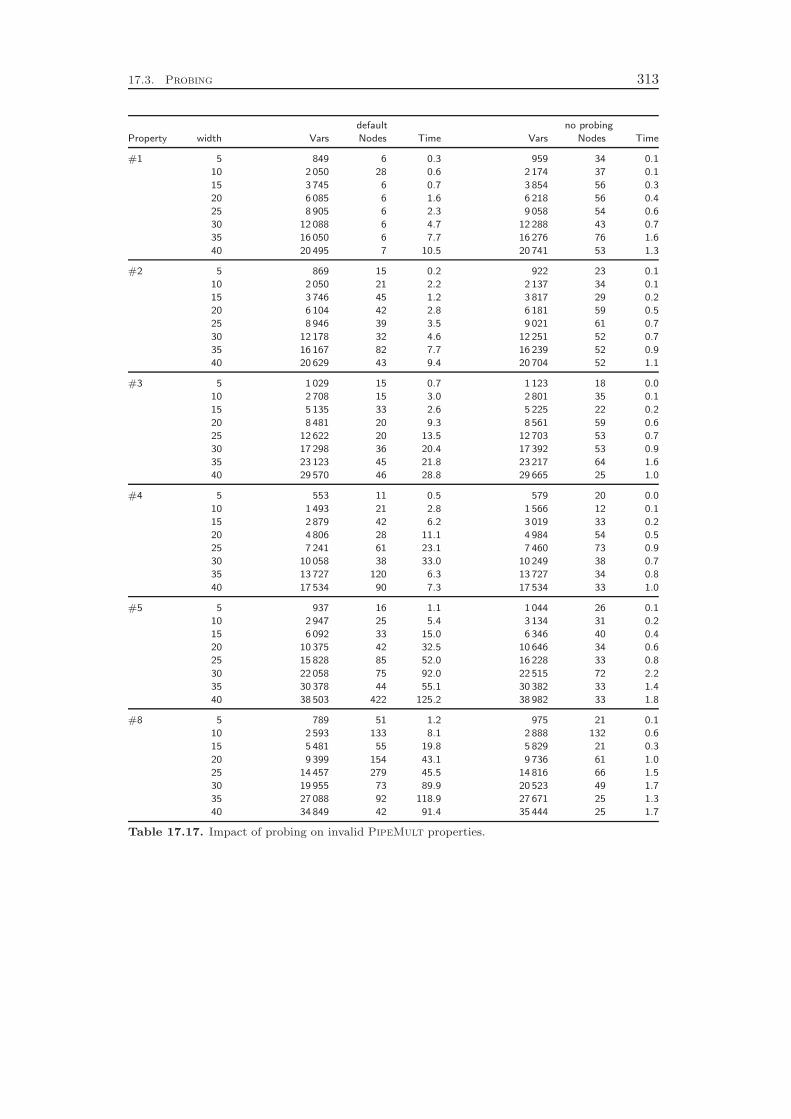
17.3. Probing 313
default no probing
Property width Vars Nodes Time Vars Nodes Time
#1 5 849 6 0.3 959 34 0.1
10 2 050 28 0.6 2 174 37 0.1
15 3 745 6 0.7 3 854 56 0.3
20 6 085 6 1.6 6 218 56 0.4
25 8 905 6 2.3 9 058 54 0.6
30 12 088 6 4.7 12 288 43 0.7
35 16 050 6 7.7 16 276 76 1.6
40 20 495 7 10.5 20 741 53 1.3
#2 5 869 15 0.2 922 23 0.1
10 2 050 21 2.2 2 137 34 0.1
15 3 746 45 1.2 3 817 29 0.2
20 6 104 42 2.8 6 181 59 0.5
25 8 946 39 3.5 9 021 61 0.7
30 12 178 32 4.6 12 251 52 0.7
35 16 167 82 7.7 16 239 52 0.9
40 20 629 43 9.4 20 704 52 1.1
#3 5 1 029 15 0.7 1 123 18 0.0
10 2 708 15 3.0 2 801 35 0.1
15 5 135 33 2.6 5 225 22 0.2
20 8 481 20 9.3 8 561 59 0.6
25 12 622 20 13.5 12 703 53 0.7
30 17 298 36 20.4 17 392 53 0.9
35 23 123 45 21.8 23 217 64 1.6
40 29 570 46 28.8 29 665 25 1.0
#4 5 553 11 0.5 579 20 0.0
10 1 493 21 2.8 1 566 12 0.1
15 2 879 42 6.2 3 019 33 0.2
20 4 806 28 11.1 4 984 54 0.5
25 7 241 61 23.1 7 460 73 0.9
30 10 058 38 33.0 10 249 38 0.7
35 13 727 120 6.3 13 727 34 0.8
40 17 534 90 7.3 17 534 33 1.0
#5 5 937 16 1.1 1 044 26 0.1
10 2 947 25 5.4 3 134 31 0.2
15 6 092 33 15.0 6 346 40 0.4
20 10 375 42 32.5 10 646 34 0.6
25 15 828 85 52.0 16 228 33 0.8
30 22 058 75 92.0 22 515 72 2.2
35 30 378 44 55.1 30 382 33 1.4
40 38 503 422 125.2 38 982 33 1.8
#8 5 789 51 1.2 975 21 0.1
10 2 593 133 8.1 2 888 132 0.6
15 5 481 55 19.8 5 829 21 0.3
20 9 399 154 43.1 9 736 61 1.0
25 14 457 279 45.5 14 816 66 1.5
30 19 955 73 89.9 20 523 49 1.7
35 27 088 92 118.9 27 671 25 1.3
40 34 849 42 91.4 35 444 25 1.7
Table 17.17. Impact of probing on invalid PipeMult properties.
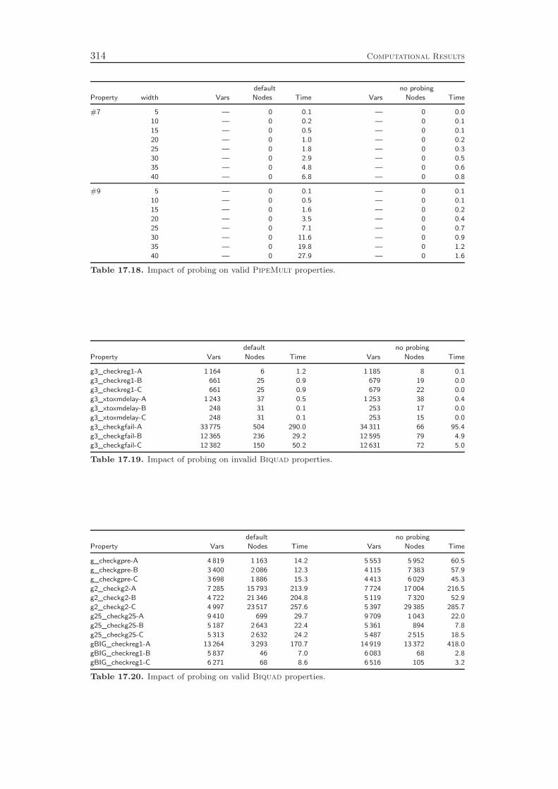
314 Computational Results
default no probing
Property width Vars Nodes Time Vars Nodes Time
#7 5 — 0 0.1 — 0 0.0
10 — 0 0.2 — 0 0.1
15 — 0 0.5 — 0 0.1
20 — 0 1.0 — 0 0.2
25 — 0 1.8 — 0 0.3
30 — 0 2.9 — 0 0.5
35 — 0 4.8 — 0 0.6
40 — 0 6.8 — 0 0.8
#9 5 — 0 0.1 — 0 0.1
10 — 0 0.5 — 0 0.1
15 — 0 1.6 — 0 0.2
20 — 0 3.5 — 0 0.4
25 — 0 7.1 — 0 0.7
30 — 0 11.6 — 0 0.9
35 — 0 19.8 — 0 1.2
40 — 0 27.9 — 0 1.6
Table 17.18. Impact of probing on valid PipeMult properties.
default no probing
Property Vars Nodes Time Vars Nodes Time
g3_checkreg1-A 1 164 6 1.2 1 185 8 0.1
g3_checkreg1-B 661 25 0.9 679 19 0.0
g3_checkreg1-C 661 25 0.9 679 22 0.0
g3_xtoxmdelay-A 1 243 37 0.5 1 253 38 0.4
g3_xtoxmdelay-B 248 31 0.1 253 17 0.0
g3_xtoxmdelay-C 248 31 0.1 253 15 0.0
g3_checkgfail-A 33 775 504 290.0 34 311 66 95.4
g3_checkgfail-B 12 365 236 29.2 12 595 79 4.9
g3_checkgfail-C 12 382 150 50.2 12 631 72 5.0
Table 17.19. Impact of probing on invalid Biquad properties.
default no probing
Property Vars Nodes Time Vars Nodes Time
g_checkgpre-A 4 819 1 163 14.2 5 553 5 952 60.5
g_checkgpre-B 3 400 2 086 12.3 4 115 7 383 57.9
g_checkgpre-C 3 698 1 886 15.3 4 413 6 029 45.3
g2_checkg2-A 7 285 15 793 213.9 7 724 17 004 216.5
g2_checkg2-B 4 722 21 346 204.8 5 119 7 320 52.9
g2_checkg2-C 4 997 23 517 257.6 5 397 29 385 285.7
g25_checkg25-A 9 410 699 29.7 9 709 1 043 22.0
g25_checkg25-B 5 187 2 643 22.4 5 361 894 7.8
g25_checkg25-C 5 313 2 632 24.2 5 487 2 515 18.5
gBIG_checkreg1-A 13 264 3 293 170.7 14 919 13 372 418.0
gBIG_checkreg1-B 5 837 46 7.0 6 083 68 2.8
gBIG_checkreg1-C 6 271 68 8.6 6 516 105 3.2
Table 17.20. Impact of probing on valid Biquad properties.
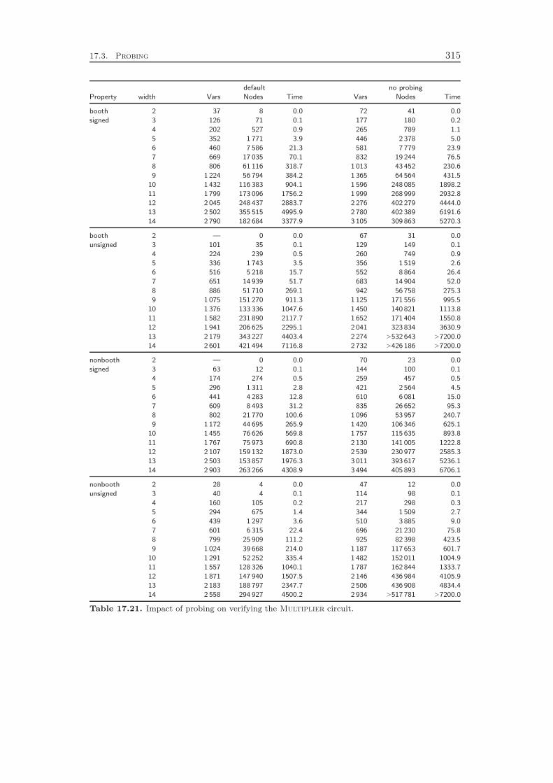
17.3. Probing 315
default no probing
Property width Vars Nodes Time Vars Nodes Time
booth 2 37 8 0.0 72 41 0.0
signed 3 126 71 0.1 177 180 0.2
4 202 527 0.9 265 789 1.1
5 352 1 771 3.9 446 2 378 5.0
6 460 7 586 21.3 581 7 779 23.9
7 669 17 035 70.1 832 19 244 76.5
8 806 61 116 318.7 1 013 43 452 230.6
9 1 224 56 794 384.2 1 365 64 564 431.5
10 1 432 116 383 904.1 1 596 248 085 1898.2
11 1 799 173 096 1756.2 1 999 268 999 2932.8
12 2 045 248 437 2883.7 2 276 402 279 4444.0
13 2 502 355 515 4995.9 2 780 402 389 6191.6
14 2 790 182 684 3377.9 3 105 309 863 5270.3
booth 2 — 0 0.0 67 31 0.0
unsigned 3 101 35 0.1 129 149 0.1
4 224 239 0.5 260 749 0.9
5 336 1 743 3.5 356 1 519 2.6
6 516 5 218 15.7 552 8 864 26.4
7 651 14 939 51.7 683 14 904 52.0
8 886 51 710 269.1 942 56 758 275.3
9 1 075 151 270 911.3 1 125 171 556 995.5
10 1 376 133 336 1047.6 1 450 140 821 1113.8
11 1 582 231 890 2117.7 1 652 171 404 1550.8
12 1 941 206 625 2295.1 2 041 323 834 3630.9
13 2 179 343 227 4403.4 2 274 >532 643 >7200.0
14 2 601 421 494 7116.8 2 732 >426 186 >7200.0
nonbooth 2 — 0 0.0 70 23 0.0
signed 3 63 12 0.1 144 100 0.1
4 174 274 0.5 259 457 0.5
5 296 1 311 2.8 421 2 564 4.5
6 441 4 283 12.8 610 6 081 15.0
7 609 8 493 31.2 835 26 652 95.3
8 802 21 770 100.6 1 096 53 957 240.7
9 1 172 44 695 265.9 1 420 106 346 625.1
10 1 455 76 626 569.8 1 757 115 635 893.8
11 1 767 75 973 690.8 2 130 141 005 1222.8
12 2 107 159 132 1873.0 2 539 230 977 2585.3
13 2 503 153 857 1976.3 3 011 393 617 5236.1
14 2 903 263 266 4308.9 3 494 405 893 6706.1
nonbooth 2 28 4 0.0 47 12 0.0
unsigned 3 40 4 0.1 114 98 0.1
4 160 105 0.2 217 298 0.3
5 294 675 1.4 344 1 509 2.7
6 439 1 297 3.6 510 3 885 9.0
7 601 6 315 22.4 696 21 230 75.8
8 799 25 909 111.2 925 82 398 423.5
9 1 024 39 668 214.0 1 187 117 653 601.7
10 1 291 52 252 335.4 1 482 152 011 1004.9
11 1 557 128 326 1040.1 1 787 162 844 1333.7
12 1 871 147 940 1507.5 2 146 436 984 4105.9
13 2 183 188 797 2347.7 2 506 436 908 4834.4
14 2 558 294 927 4500.2 2 934 >517 781 >7200.0
Table 17.21. Impact of probing on verifying the Multiplier circuit.

316 Computational Results
default no conflict analysis
Property width Nodes Time Nodes Time
neg_flag 5 45 0.8 309 0.9
10 50 3.6 619 4.1
15 64 11.6 597 11.7
20 42 36.3 939 36.9
25 107 81.8 573 80.9
30 53 136.6 885 139.0
35 35 218.4 1 665 225.5
40 55 383.5 1 991 387.3
zero_flag 5 54 2.3 141 2.3
10 28 0.6 45 0.7
15 37 1.6 83 1.6
20 26 4.0 57 3.3
25 78 6.2 185 6.2
30 73 10.7 197 10.6
35 63 15.6 129 15.1
40 185 379.7 2 715 421.4
Table 17.22. Impact of conflict analysis on valid ALU properties.
17.4 Conflict Analysis
Conflict analysis is a technique to analyze infeasible subproblems that are encoun-tered during the branch-and-bound search. It can produce additional valid con-straints that can be used later in the solving process to prune the search tree.Conflict analysis has originated in the SAT community and is particularly suitedfor proving the infeasibility of a problem instance. Chapter 11 explains how conflictanalysis can be generalized to mixed integer programming, which easily extends toconstraint integer programming.
In order to use conflict analysis for arbitrary constraints, each constraint handlerhas to implement a so-called reverse propagation method. This method has to pro-vide the “reasons” for a deduction that the constraint handler’s domain propagationmethod has produced earlier during the search, compare Section 11.1. Given therather complex domain propagation algorithms of our chip verification constrainthandlers, this is not an easy task. Nevertheless, we equipped the constraint han-dlers with the necessary algorithms such that almost all of the possible propagationscan be “reverse propagated”.
In this section, we evaluate the impact of conflict analysis on solving propertychecking problems. Since counter-examples to the invalid ALU properties can befound in at most 4 branch-and-bound nodes, conflict analysis does not have anyinfluence on these instances. The same holds for all instances that can already besolved in the presolving stage, which includes the muls property of the ALU circuit.The results for the remaining two valid ALU instances are shown in Table 17.22.It turns out that the number of branching nodes needed to prove the infeasibilityof the instances gets significantly larger if conflict analysis is disabled. This doesnot, however, increase the runtime by a significant amount. In fact, almost all ofthe runtime is spent in presolving, such that the time that can be saved by conflictanalysis is very limited.
Similar to the invalid ALU instances, finding counter-examples for the invalidPipeAdder and PipeMult properties is so easy that conflict analysis cannot yieldsignificant performance improvements. The correctness of the valid properties ofthese circuits is already shown in presolving. Therefore, we skip the tables with thePipeAdder and PipeMult results.
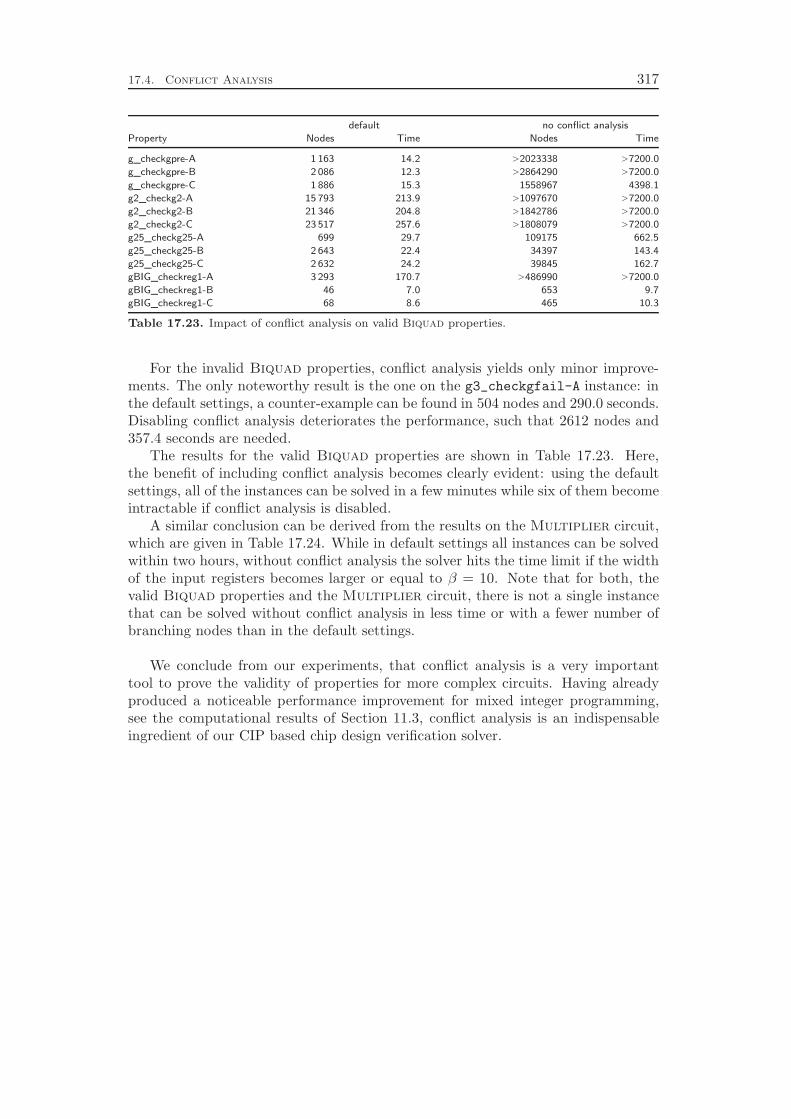
17.4. Conflict Analysis 317
default no conflict analysis
Property Nodes Time Nodes Time
g_checkgpre-A 1 163 14.2 >2023338 >7200.0
g_checkgpre-B 2 086 12.3 >2864290 >7200.0
g_checkgpre-C 1 886 15.3 1558967 4398.1
g2_checkg2-A 15 793 213.9 >1097670 >7200.0
g2_checkg2-B 21 346 204.8 >1842786 >7200.0
g2_checkg2-C 23 517 257.6 >1808079 >7200.0
g25_checkg25-A 699 29.7 109175 662.5
g25_checkg25-B 2 643 22.4 34397 143.4
g25_checkg25-C 2 632 24.2 39845 162.7
gBIG_checkreg1-A 3 293 170.7 >486990 >7200.0
gBIG_checkreg1-B 46 7.0 653 9.7
gBIG_checkreg1-C 68 8.6 465 10.3
Table 17.23. Impact of conflict analysis on valid Biquad properties.
For the invalid Biquad properties, conflict analysis yields only minor improve-ments. The only noteworthy result is the one on the g3_checkgfail-A instance: inthe default settings, a counter-example can be found in 504 nodes and 290.0 seconds.Disabling conflict analysis deteriorates the performance, such that 2612 nodes and357.4 seconds are needed.
The results for the valid Biquad properties are shown in Table 17.23. Here,the benefit of including conflict analysis becomes clearly evident: using the defaultsettings, all of the instances can be solved in a few minutes while six of them becomeintractable if conflict analysis is disabled.
A similar conclusion can be derived from the results on the Multiplier circuit,which are given in Table 17.24. While in default settings all instances can be solvedwithin two hours, without conflict analysis the solver hits the time limit if the widthof the input registers becomes larger or equal to β = 10. Note that for both, thevalid Biquad properties and the Multiplier circuit, there is not a single instancethat can be solved without conflict analysis in less time or with a fewer number ofbranching nodes than in the default settings.
We conclude from our experiments, that conflict analysis is a very importanttool to prove the validity of properties for more complex circuits. Having alreadyproduced a noticeable performance improvement for mixed integer programming,see the computational results of Section 11.3, conflict analysis is an indispensableingredient of our CIP based chip design verification solver.
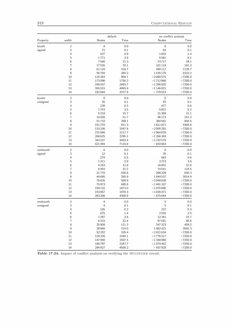
318 Computational Results
default no conflict analysis
Property width Nodes Time Nodes Time
booth 2 8 0.0 9 0.0
signed 3 71 0.1 83 0.1
4 527 0.9 1 603 1.4
5 1 771 3.9 5 581 6.1
6 7 586 21.3 23 717 34.1
7 17 035 70.1 101 119 181.3
8 61 116 318.7 499 117 1129.7
9 56 794 384.2 1 435 175 4322.2
10 116 383 904.1 >2 080 575 >7200.0
11 173 096 1756.2 >1 712 966 >7200.0
12 248 437 2883.7 >1 298 920 >7200.0
13 355 515 4995.9 >1 146 821 >7200.0
14 182 684 3377.9 > 729 553 >7200.0
booth 2 0 0.0 0 0.0
unsigned 3 35 0.1 55 0.1
4 239 0.5 477 0.6
5 1 743 3.5 5 821 6.2
6 5 218 15.7 21 389 31.1
7 14 939 51.7 96 173 151.2
8 51 710 269.1 384 581 858.5
9 151 270 911.3 1 811 671 4469.6
10 133 336 1047.6 >2 005 291 >7200.0
11 231 890 2117.7 >1 964 676 >7200.0
12 206 625 2295.1 >1 266 363 >7200.0
13 343 227 4403.4 >1 232 579 >7200.0
14 421 494 7116.8 > 834 663 >7200.0
nonbooth 2 0 0.0 0 0.0
signed 3 12 0.1 25 0.1
4 274 0.5 563 0.6
5 1 311 2.8 3 273 3.6
6 4 283 12.8 16 951 22.8
7 8 493 31.2 74 541 124.5
8 21 770 100.6 298 209 640.3
9 44 695 265.9 1 044 537 3014.9
10 76 626 569.8 >2 048 638 >7200.0
11 75 973 690.8 >1 491 337 >7200.0
12 159 132 1873.0 >1 075 690 >7200.0
13 153 857 1976.3 >1 026 471 >7200.0
14 263 266 4308.9 > 675 644 >7200.0
nonbooth 2 4 0.0 5 0.0
unsigned 3 4 0.1 5 0.1
4 105 0.2 237 0.3
5 675 1.4 2 535 2.5
6 1 297 3.6 12 341 15.7
7 6 315 22.4 67 581 96.6
8 25 909 111.2 247 323 459.2
9 39 668 214.0 1 082 421 2691.3
10 52 252 335.4 >2 421 634 >7200.0
11 128 326 1040.1 >1 776 217 >7200.0
12 147 940 1507.5 >1 348 860 >7200.0
13 188 797 2347.7 >1 074 452 >7200.0
14 294 927 4500.2 > 937 928 >7200.0
Table 17.24. Impact of conflict analysis on verifying the Multiplier circuit.
Appendix A
Computational Environment
In the following we characterize the computational infrastructure and the environ-ment under which our computational experiments have been conducted. Afterwards,we describe the various test sets on which the computations have been performed.
A.1 Computational Infrastructure
All benchmark runs have been executed on Dell Precision 370 desktop PCs with2 GB RAM and a 3.8 GHz Intel Pentium 4 CPU with 1 MB second-level cache.They have been distributed to eight equivalent machines. We used Suse Linux 10.2as operating system and Gcc 4.1.2 with the -O3 optimizer option to compile thesource code.
All timings are reported in CPU seconds. As time measurements, in particularfor hyperthreading CPUs, are very dependent on the CPU load caused by otherprocesses running in the background, the author did his best to run the tests onlyon unloaded machines and to rerun suspicious benchmarks. Small variations in theruntime, however, cannot be avoided. Our experience for the reported mean valuesis that differences of up to 2 % in the average runtime can be attributed to variationsin the timing.
For the MIP benchmarks, we used a time limit of one hour, while we allowed twohour runs on the chip verification test sets. If the time limit was hit, we treat thetime limit and the current number of processed nodes as the resulting benchmarkvalues. Thus, we pretend that the instance was solved at this moment. Note thatthis provides an advantage to the runs in which the time limit was hit, since theaccounted values are smaller than the actual time and number of nodes neededto solve the respective instances. On the other hand, it has the benefit that theinfluence on the overall statistics due to a failure on a single instance is limited.
We imposed a memory limit of 1.5 GB in order to avoid swapping. If the memorylimit was hit, we treat the run as if it hit the time limit. The accounted number ofnodes is scaled accordingly, as if the nodes per time ratio stayed constant throughoutthe solving process. An excess of the memory limit happened only very infrequentlyin our computations. In total, only 180 out of the 28060 MIP runs have beenaborted due to the memory limit, most of them for the mik test set, in particularwith random branching , most infeasible branching , least infeasible branching , andinference branching . All of the chip verification runs stayed within the memorylimit.
We used two unofficial versions of SCIP in the benchmark runs that the authorwill make available on request. For the MIP benchmarks, we employed SCIP 0.90f,while the chip verification benchmarks have been conducted using SCIP 0.90i asCIP framework. SCIP 0.90i is the more recent version of the two. It is very similarto version 1.0, which will be published shortly after this thesis. We linked SCIP toCplex 10.0.1 [118] in order to solve the underlying LP relaxations.
319
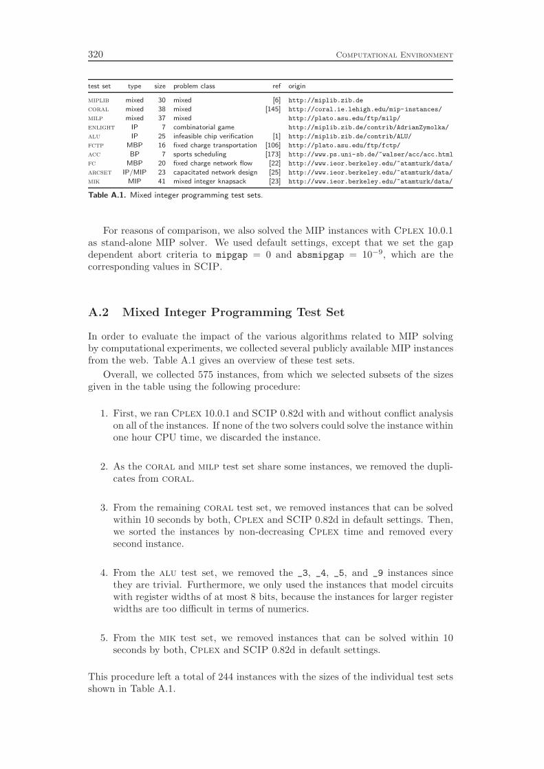
320 Computational Environment
test set type size problem class ref origin
miplib mixed 30 mixed [6] http://miplib.zib.de
coral mixed 38 mixed [145] http://coral.ie.lehigh.edu/mip-instances/
milp mixed 37 mixed http://plato.asu.edu/ftp/milp/
enlight IP 7 combinatorial game http://miplib.zib.de/contrib/AdrianZymolka/
alu IP 25 infeasible chip verification [1] http://miplib.zib.de/contrib/ALU/
fctp MBP 16 fixed charge transportation [106] http://plato.asu.edu/ftp/fctp/
acc BP 7 sports scheduling [173] http://www.ps.uni-sb.de/~walser/acc/acc.html
fc MBP 20 fixed charge network flow [22] http://www.ieor.berkeley.edu/~atamturk/data/
arcset IP/MIP 23 capacitated network design [25] http://www.ieor.berkeley.edu/~atamturk/data/
mik MIP 41 mixed integer knapsack [23] http://www.ieor.berkeley.edu/~atamturk/data/
Table A.1. Mixed integer programming test sets.
For reasons of comparison, we also solved the MIP instances with Cplex 10.0.1as stand-alone MIP solver. We used default settings, except that we set the gapdependent abort criteria to mipgap = 0 and absmipgap = 10−9, which are thecorresponding values in SCIP.
A.2 Mixed Integer Programming Test Set
In order to evaluate the impact of the various algorithms related to MIP solvingby computational experiments, we collected several publicly available MIP instancesfrom the web. Table A.1 gives an overview of these test sets.
Overall, we collected 575 instances, from which we selected subsets of the sizesgiven in the table using the following procedure:
1. First, we ran Cplex 10.0.1 and SCIP 0.82d with and without conflict analysison all of the instances. If none of the two solvers could solve the instance withinone hour CPU time, we discarded the instance.
2. As the coral and milp test set share some instances, we removed the dupli-cates from coral.
3. From the remaining coral test set, we removed instances that can be solvedwithin 10 seconds by both, Cplex and SCIP 0.82d in default settings. Then,we sorted the instances by non-decreasing Cplex time and removed everysecond instance.
4. From the alu test set, we removed the _3, _4, _5, and _9 instances sincethey are trivial. Furthermore, we only used the instances that model circuitswith register widths of at most 8 bits, because the instances for larger registerwidths are too difficult in terms of numerics.
5. From the mik test set, we removed instances that can be solved within 10seconds by both, Cplex and SCIP 0.82d in default settings.
This procedure left a total of 244 instances with the sizes of the individual test setsshown in Table A.1.
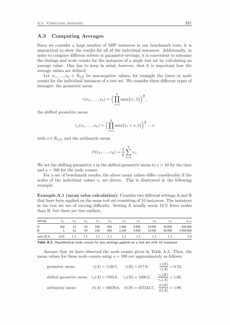
A.3. Computing Averages 321
A.3 Computing Averages
Since we consider a large number of MIP instances in our benchmark tests, it isunpractical to show the results for all of the individual instances. Additionally, inorder to compare different solvers or parameter settings, it is convenient to subsumethe timings and node counts for the instances of a single test set by calculating anaverage value. One has to keep in mind, however, that it is important how theaverage values are defined.
Let v1, . . . , vk ∈ R≥0 be non-negative values, for example the times or nodecounts for the individual instances of a test set. We consider three different types ofaverages: the geometric mean
γ(v1, . . . , vk) =( k∏
i=1
max{vi, 1}) 1
k
,
the shifted geometric mean
γs(v1, . . . , vk) =( k∏
i=1
max{vi + s, 1}) 1
k
− s
with s ∈ R≥0, and the arithmetic mean
∅(v1, . . . , vk) =1
k
k∑
i=1
vi.
We set the shifting parameter s in the shifted geometric mean to s = 10 for the timeand s = 100 for the node counts.
For a set of benchmark results, the above mean values differ considerably if thescales of the individual values vi are divers. This is illustrated in the followingexample:
Example A.1 (mean value calculation). Consider two different settings A and Bthat have been applied on the same test set consisting of 10 instances. The instancesin the test set are of varying difficulty. Setting A usually needs 10 % fewer nodesthan B, but there are two outliers.
setting n1 n2 n3 n4 n5 n6 n7 n8 n9 n10
A 100 10 50 100 500 1 000 5 000 10 000 50 000 500 000
B 1 11 55 110 550 1 100 5 500 11 000 55 000 1 000 000
ratio B/A 0.01 1.1 1.1 1.1 1.1 1.1 1.1 1.1 1.1 2.0
Table A.2. Hypothetical node counts for two settings applied on a test set with 10 instances.
Assume that we have observed the node counts given in Table A.2. Then, themean values for these node counts using s = 100 are approximately as follows:
geometric mean: γ(A) = 1120.7, γ(B) = 817.9,γ(B)
γ(A)= 0.73,
shifted geometric mean: γs(A) = 1783.6, γs(B) = 1890.2,γs(B)
γs(A)= 1.06,
arithmetic mean: ∅(A) = 56676.0, ∅(B) = 107332.7,∅(B)
∅(A)= 1.89.
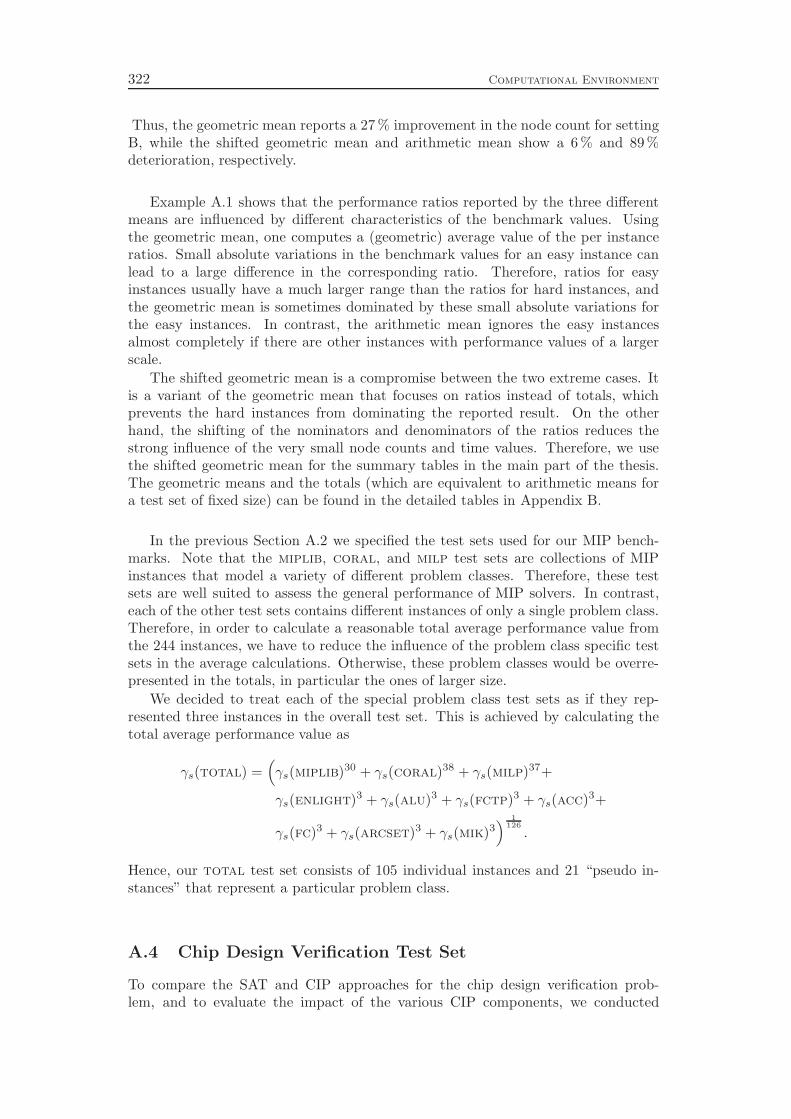
322 Computational Environment
Thus, the geometric mean reports a 27 % improvement in the node count for settingB, while the shifted geometric mean and arithmetic mean show a 6 % and 89 %deterioration, respectively.
Example A.1 shows that the performance ratios reported by the three differentmeans are influenced by different characteristics of the benchmark values. Usingthe geometric mean, one computes a (geometric) average value of the per instanceratios. Small absolute variations in the benchmark values for an easy instance canlead to a large difference in the corresponding ratio. Therefore, ratios for easyinstances usually have a much larger range than the ratios for hard instances, andthe geometric mean is sometimes dominated by these small absolute variations forthe easy instances. In contrast, the arithmetic mean ignores the easy instancesalmost completely if there are other instances with performance values of a largerscale.
The shifted geometric mean is a compromise between the two extreme cases. Itis a variant of the geometric mean that focuses on ratios instead of totals, whichprevents the hard instances from dominating the reported result. On the otherhand, the shifting of the nominators and denominators of the ratios reduces thestrong influence of the very small node counts and time values. Therefore, we usethe shifted geometric mean for the summary tables in the main part of the thesis.The geometric means and the totals (which are equivalent to arithmetic means fora test set of fixed size) can be found in the detailed tables in Appendix B.
In the previous Section A.2 we specified the test sets used for our MIP bench-marks. Note that the miplib, coral, and milp test sets are collections of MIPinstances that model a variety of different problem classes. Therefore, these testsets are well suited to assess the general performance of MIP solvers. In contrast,each of the other test sets contains different instances of only a single problem class.Therefore, in order to calculate a reasonable total average performance value fromthe 244 instances, we have to reduce the influence of the problem class specific testsets in the average calculations. Otherwise, these problem classes would be overre-presented in the totals, in particular the ones of larger size.
We decided to treat each of the special problem class test sets as if they rep-resented three instances in the overall test set. This is achieved by calculating thetotal average performance value as
γs(total) =(
γs(miplib)30 + γs(coral)38 + γs(milp)37+
γs(enlight)3 + γs(alu)3 + γs(fctp)3 + γs(acc)3+
γs(fc)3 + γs(arcset)3 + γs(mik)3) 1
126
.
Hence, our total test set consists of 105 individual instances and 21 “pseudo in-stances” that represent a particular problem class.
A.4 Chip Design Verification Test Set
To compare the SAT and CIP approaches for the chip design verification prob-lem, and to evaluate the impact of the various CIP components, we conducted

A.4. Chip Design Verification Test Set 323
experiments on the following sets of property checking instances, which have beengenerated by OneSpin Solutions:
⊲ ALU: an arithmetical logical unit which is able to perform add, sub, shl,shr, and signed and unsigned mult operations.
⊲ PipeAdder: an adder with a 4-stage pipeline to add up four values.
⊲ PipeMult: a multiplier with a 4-stage pipeline to multiply four values.
⊲ Biquad: a DSP/IIR filter core obtained from [177] in different representationswith some valid and invalid properties.
⊲ Multiplier: boothed and non-boothed gate level architectures of signed andunsigned multiplication networks, for which the correctness has to be proven.These instances are rather equivalence checking instances than property check-ing problems.
All test sets except the Multiplier set involve valid and invalid properties. Thewidth of the input registers in the ALU, PipeAdder and PipeMult sets rangefrom 5 to 40 bits. For the Multiplier instances the width ranges from 2 to 14 bits.
We converted these instances into a register transfer level description and anequivalent gate level representation using proprietary tools of OneSpin Solutions.The former representation is used as input for our CIP solver, the latter for a SATsolver.
Note that the tools of OneSpin Solutions perform an additional presolvingstep during the transformation to the gate level, which can simplify or sometimeseven completely solve the instances. Therefore, some instances are not available asSAT input, which is marked by reporting a node count of 0 and a runtime of 0.0 inthe benchmark results. The time needed for the gate level transformation and thepresolving is not included in the timings reported in the result tables. However, thistime is usually neglectable.


Appendix B
Tables
This appendix chapter presents detailed result tables for our benchmark tests onmixed integer programming. Each table contains statistics for using various differentparameter settings on the instances of a single test set. The column “setting” lists thesettings that we have tried. In column “T” one can find the number of instances forwhich the solver hit the time or memory limit if called with the respective parametersettings. The columns “fst” and “slw” indicate, how many instances have been solvedat least 10 % faster or slower, respectively, than with the reference settings of thefirst row (which usually are the default settings).
The ngm, nsgm, and ntot values represent the geometric means, shifted geometricmeans, and total numbers of branching nodes, respectively, that have been spent onsolving the instances of the test set. The numbers are given as percental relativedifferences to the reference settings: if S0 are the reference settings, the number incolumn ngm for setting i is equal to
nigm = 100 ·
(
γ(ni1, . . . , n
ik)
γ(n01, . . . , n
0k)− 1
)
, (B.1)
with nij being the node count on instance j for settings Si. Analogous formulas are
used for the other entries of the table.The tgm, tsgm, and ttot values are the geometric means, shifted geometric means,
and totals of the time needed to solve the instances of the test set. Again, we listpercental relative differences to the reference settings that are calculated in a similarway as in Equation (B.1). Note that the numbers shown in the summary tables inthe main part of the thesis are the shifted geometric means, i.e., we have copiedcolumns nsgm and tsgm of the “all instances” block into the summary tables.
In order to evaluate the impact and the computational costs of a certain strategy,it is sometimes useful to distinguish between the models that are affected by thechange in the solving strategy and the ones for which the solving process proceedsin exactly the same way as for the reference settings. This distinction yields the“different path” and “equal path” blocks of the tables. While the “all instances”block shows the average values for all instances in the test set (with the numberof instances indicated in brackets), the average values in the “different path” blockare calculated on only those instances for which the solving path for the respectivesettings is different to the one of the reference settings. Since it is very hard toactually compare the paths in the search tree, we assume that the solving path oftwo runs is equal if and only if both runs spent the same number of branching nodesand the same total number of simplex iterations to process the instance. Of course,this may declare some runs to have the same path although they were different.However, this seems to be very unlikely.
The “#” columns in these blocks show the number of instances that fall intothe respective category. Note that we only include instances that were solved tooptimality within the time and memory limit by both, the reference settings and thesettings of the respective row. Therefore, the sum of the “different” and “equal path”
325

326 Tables
instances is only equal to the total number of instances in the test set if none of thetwo involved settings hit the time or memory limit. Note also that the comparisonof the different settings does not make sense in the “different path” and “equal path”blocks, since the values are usually averages over a different subset of the instances.
The full tables with all results of the individual instances and the complete logfiles of the runs can be found in the web at http://scip.zib.de.
Memory Management
all instances (30) different path equal path
setting T fst slw ngm nsgm ntot tgm tsgm ttot # tgm tsgm ttot # tgm tsgm ttot
default 1 0 0 0 0 0 0 0 0 0 — — — 29 0 0 0
no block 2 0 9 −1 −1 −7 +9 +8 +16 0 — — — 28 +8 +7 +15
no buffer 1 1 5 0 0 −1 +6 +3 +1 0 — — — 29 +6 +3 +2
none 2 0 7 −1 −1 −7 +7 +6 +15 0 — — — 28 +6 +5 +12
Table B.1. Evaluation of memory management on test set miplib.
all instances (38) different path equal path
setting T fst slw ngm nsgm ntot tgm tsgm ttot # tgm tsgm ttot # tgm tsgm ttot
default 3 0 0 0 0 0 0 0 0 0 — — — 35 0 0 0
no block 3 0 13 0 0 −1 +10 +10 +10 0 — — — 35 +11 +11 +19
no buffer 3 0 0 0 0 0 0 0 0 0 — — — 35 0 0 0
none 3 0 13 0 0 −1 +12 +11 +12 0 — — — 35 +13 +12 +24
Table B.2. Evaluation of memory management on test set coral.
all instances (36) different path equal path
setting T fst slw ngm nsgm ntot tgm tsgm ttot # tgm tsgm ttot # tgm tsgm ttot
default 7 0 0 0 0 0 0 0 0 0 — — — 29 0 0 0
no block 7 0 10 −1 −1 −7 +8 +7 +4 0 — — — 29 +10 +9 +10
no buffer 7 0 0 0 0 0 −1 −1 0 0 — — — 29 −1 −1 −1
none 7 0 10 −1 −1 −7 +7 +7 +3 0 — — — 29 +9 +8 +9
Table B.3. Evaluation of memory management on test set milp.
all instances (7) different path equal path
setting T fst slw ngm nsgm ntot tgm tsgm ttot # tgm tsgm ttot # tgm tsgm ttot
default 0 0 0 0 0 0 0 0 0 0 — — — 7 0 0 0
no block 0 0 0 0 0 0 +4 +3 +8 0 — — — 7 +4 +3 +8
no buffer 0 0 0 0 0 0 +1 −1 −2 0 — — — 7 +1 −1 −2
none 0 0 3 0 0 0 +11 +7 +19 0 — — — 7 +11 +7 +19
Table B.4. Evaluation of memory management on test set enlight.
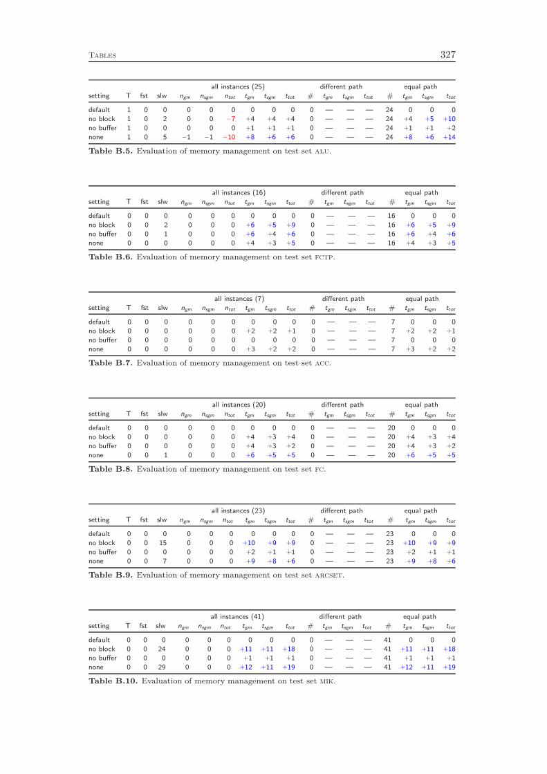
Tables 327
all instances (25) different path equal path
setting T fst slw ngm nsgm ntot tgm tsgm ttot # tgm tsgm ttot # tgm tsgm ttot
default 1 0 0 0 0 0 0 0 0 0 — — — 24 0 0 0
no block 1 0 2 0 0 −7 +4 +4 +4 0 — — — 24 +4 +5 +10
no buffer 1 0 0 0 0 0 +1 +1 +1 0 — — — 24 +1 +1 +2
none 1 0 5 −1 −1 −10 +8 +6 +6 0 — — — 24 +8 +6 +14
Table B.5. Evaluation of memory management on test set alu.
all instances (16) different path equal path
setting T fst slw ngm nsgm ntot tgm tsgm ttot # tgm tsgm ttot # tgm tsgm ttot
default 0 0 0 0 0 0 0 0 0 0 — — — 16 0 0 0
no block 0 0 2 0 0 0 +6 +5 +9 0 — — — 16 +6 +5 +9
no buffer 0 0 1 0 0 0 +6 +4 +6 0 — — — 16 +6 +4 +6
none 0 0 0 0 0 0 +4 +3 +5 0 — — — 16 +4 +3 +5
Table B.6. Evaluation of memory management on test set fctp.
all instances (7) different path equal path
setting T fst slw ngm nsgm ntot tgm tsgm ttot # tgm tsgm ttot # tgm tsgm ttot
default 0 0 0 0 0 0 0 0 0 0 — — — 7 0 0 0
no block 0 0 0 0 0 0 +2 +2 +1 0 — — — 7 +2 +2 +1
no buffer 0 0 0 0 0 0 0 0 0 0 — — — 7 0 0 0
none 0 0 0 0 0 0 +3 +2 +2 0 — — — 7 +3 +2 +2
Table B.7. Evaluation of memory management on test set acc.
all instances (20) different path equal path
setting T fst slw ngm nsgm ntot tgm tsgm ttot # tgm tsgm ttot # tgm tsgm ttot
default 0 0 0 0 0 0 0 0 0 0 — — — 20 0 0 0
no block 0 0 0 0 0 0 +4 +3 +4 0 — — — 20 +4 +3 +4
no buffer 0 0 0 0 0 0 +4 +3 +2 0 — — — 20 +4 +3 +2
none 0 0 1 0 0 0 +6 +5 +5 0 — — — 20 +6 +5 +5
Table B.8. Evaluation of memory management on test set fc.
all instances (23) different path equal path
setting T fst slw ngm nsgm ntot tgm tsgm ttot # tgm tsgm ttot # tgm tsgm ttot
default 0 0 0 0 0 0 0 0 0 0 — — — 23 0 0 0
no block 0 0 15 0 0 0 +10 +9 +9 0 — — — 23 +10 +9 +9
no buffer 0 0 0 0 0 0 +2 +1 +1 0 — — — 23 +2 +1 +1
none 0 0 7 0 0 0 +9 +8 +6 0 — — — 23 +9 +8 +6
Table B.9. Evaluation of memory management on test set arcset.
all instances (41) different path equal path
setting T fst slw ngm nsgm ntot tgm tsgm ttot # tgm tsgm ttot # tgm tsgm ttot
default 0 0 0 0 0 0 0 0 0 0 — — — 41 0 0 0
no block 0 0 24 0 0 0 +11 +11 +18 0 — — — 41 +11 +11 +18
no buffer 0 0 0 0 0 0 +1 +1 +1 0 — — — 41 +1 +1 +1
none 0 0 29 0 0 0 +12 +11 +19 0 — — — 41 +12 +11 +19
Table B.10. Evaluation of memory management on test set mik.

328 Tables
Branching
all instances (30) different path equal path
setting T fst slw ngm nsgm ntot tgm tsgm ttot # tgm tsgm ttot # tgm tsgm ttot
default 1 0 0 0 0 0 0 0 0 0 — — — 29 0 0 0
random 8 1 22 +808 +475 +42 +162 +139 +180 19 +134 +112 +227 3 −2 −1 −1
most inf 7 2 20 +569 +341 +16 +153 +139 +169 20 +147 +139 +356 3 −2 −2 −2
least inf 10 1 22 +1804 +1096 +100 +325 +266 +268 17 +322 +268 +790 3 0 0 0
pseudocost 1 5 13 +183 +87 −11 +20 +16 +27 26 +23 +19 +40 3 0 0 0
full strong 3 1 18 −71 −65 −82 +95 +92 +128 24 +107 +105 +165 3 −1 0 0
strong 2 1 13 −64 −62 −78 +38 +38 +46 19 +52 +49 +36 9 +1 +1 0
hybr strong 1 2 11 −24 −18 +3 +19 +20 +23 22 +27 +27 +34 7 −1 −1 −2
psc strinit 1 8 6 +31 +13 −2 +5 +5 −3 25 +6 +6 −5 4 −2 −1 −2
reliability 1 4 4 −10 −7 −9 −1 −1 −6 21 −1 −1 −8 8 −1 −1 −1
inference 7 1 20 +483 +269 +53 +108 +101 +171 20 +84 +79 +377 3 0 0 0
Table B.11. Evaluation of branching on test set miplib.
all instances (37) different path equal path
setting T fst slw ngm nsgm ntot tgm tsgm ttot # tgm tsgm ttot # tgm tsgm ttot
default 2 0 0 0 0 0 0 0 0 0 — — — 35 0 0 0
random 18 4 27 +758 +694 +148 +332 +332 +298 17 +114 +123 +222 2 0 0 0
most inf 15 4 26 +529 +517 +125 +312 +314 +275 20 +132 +141 +232 2 +1 +1 +1
least inf 21 2 29 +1586 +1380 +195 +598 +575 +369 14 +242 +238 +330 2 −2 −2 −1
pseudocost 3 9 19 +84 +79 +68 +38 +40 +50 31 +37 +39 +70 2 0 0 +1
full strong 4 3 28 −85 −79 −34 +98 +97 +86 30 +115 +114 +115 2 −2 −2 −1
strong 3 2 23 −73 −68 −35 +59 +59 +65 31 +68 +69 +96 3 −1 −1 −1
hybr strong 4 8 14 −19 −12 +32 +27 +27 +43 31 +16 +16 +28 2 +1 +1 +2
psc strinit 1 14 9 +17 +18 −18 +2 +2 −7 33 +6 +6 +11 2 −2 −2 −1
reliability 2 11 8 +14 +16 −14 +6 +7 +13 31 +7 +8 +23 4 +2 +2 +2
inference 12 4 25 +381 +329 +105 +179 +177 +192 23 +103 +103 +153 2 −1 0 0
Table B.12. Evaluation of branching on test set coral.
all instances (35) different path equal path
setting T fst slw ngm nsgm ntot tgm tsgm ttot # tgm tsgm ttot # tgm tsgm ttot
default 6 0 0 0 0 0 0 0 0 0 — — — 29 0 0 0
random 14 5 16 +304 +194 +19 +86 +81 +65 16 +48 +41 +47 5 +1 0 +1
most inf 16 5 16 +269 +187 +22 +93 +86 +75 14 +14 +6 −6 5 0 0 0
least inf 16 5 16 +488 +306 +32 +113 +109 +84 14 +47 +42 +53 5 0 0 0
pseudocost 10 7 13 +105 +71 +18 +23 +23 +30 20 +17 +15 +35 5 −1 −1 −1
full strong 12 4 19 −79 −72 −68 +115 +107 +72 15 +198 +177 +212 5 0 0 +1
strong 7 4 18 −58 −59 −80 +46 +44 +22 17 +111 +105 +99 9 +2 +1 +1
hybr strong 10 1 18 +45 +41 +24 +47 +43 +33 17 +73 +64 +66 8 0 0 −1
psc strinit 8 7 8 +37 +40 +9 +8 +9 +14 18 −1 0 −1 9 0 0 0
reliability 6 7 8 +11 +7 −4 +5 +6 +7 17 +4 +6 +6 10 +1 +1 +2
inference 8 8 11 +122 +76 +1 +20 +20 +25 21 +25 +26 +67 5 −2 −1 0
Table B.13. Evaluation of branching on test set milp.
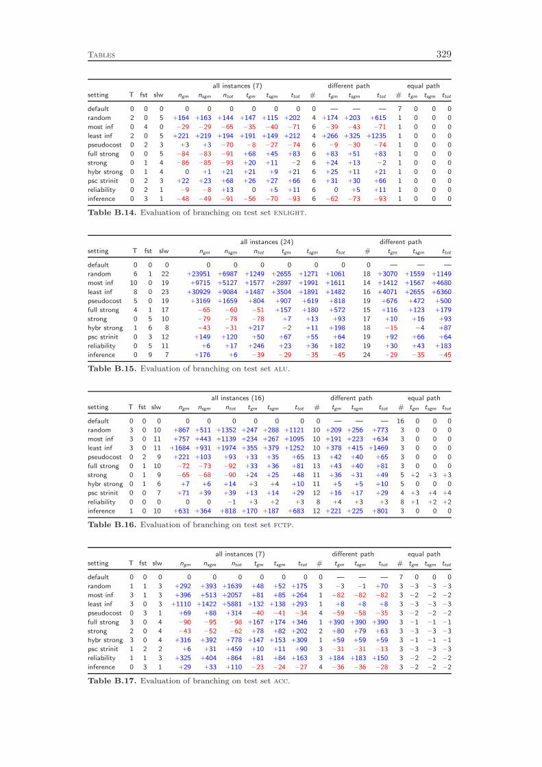
Tables 329
all instances (7) different path equal path
setting T fst slw ngm nsgm ntot tgm tsgm ttot # tgm tsgm ttot # tgm tsgm ttot
default 0 0 0 0 0 0 0 0 0 0 — — — 7 0 0 0
random 2 0 5 +164 +163 +144 +147 +115 +202 4 +174 +203 +615 1 0 0 0
most inf 0 4 0 −29 −29 −65 −35 −40 −71 6 −39 −43 −71 1 0 0 0
least inf 2 0 5 +221 +219 +194 +191 +149 +212 4 +266 +325 +1235 1 0 0 0
pseudocost 0 2 3 +3 +3 −70 −8 −27 −74 6 −9 −30 −74 1 0 0 0
full strong 0 0 5 −84 −83 −91 +68 +45 +83 6 +83 +51 +83 1 0 0 0
strong 0 1 4 −86 −85 −93 +20 +11 −2 6 +24 +13 −2 1 0 0 0
hybr strong 0 1 4 0 +1 +21 +21 +9 +21 6 +25 +11 +21 1 0 0 0
psc strinit 0 2 3 +22 +23 +68 +26 +27 +66 6 +31 +30 +66 1 0 0 0
reliability 0 2 1 −9 −8 +13 0 +5 +11 6 0 +5 +11 1 0 0 0
inference 0 3 1 −48 −49 −91 −56 −70 −93 6 −62 −73 −93 1 0 0 0
Table B.14. Evaluation of branching on test set enlight.
all instances (24) different path
setting T fst slw ngm nsgm ntot tgm tsgm ttot # tgm tsgm ttot
default 0 0 0 0 0 0 0 0 0 0 — — —
random 6 1 22 +23951 +6987 +1249 +2655 +1271 +1061 18 +3070 +1559 +1149
most inf 10 0 19 +9715 +5127 +1577 +2897 +1991 +1611 14 +1412 +1567 +4680
least inf 8 0 23 +30929 +9084 +1487 +3504 +1891 +1482 16 +4071 +2655 +6360
pseudocost 5 0 19 +3169 +1659 +804 +907 +619 +818 19 +676 +472 +500
full strong 4 1 17 −65 −60 −51 +157 +180 +572 15 +116 +123 +179
strong 0 5 10 −79 −78 −78 +7 +13 +93 17 +10 +16 +93
hybr strong 1 6 8 −43 −31 +217 −2 +11 +198 18 −15 −4 +87
psc strinit 0 3 12 +149 +120 +50 +67 +55 +64 19 +92 +66 +64
reliability 0 5 11 +6 +17 +246 +23 +36 +182 19 +30 +43 +183
inference 0 9 7 +176 +6 −39 −29 −35 −45 24 −29 −35 −45
Table B.15. Evaluation of branching on test set alu.
all instances (16) different path equal path
setting T fst slw ngm nsgm ntot tgm tsgm ttot # tgm tsgm ttot # tgm tsgm ttot
default 0 0 0 0 0 0 0 0 0 0 — — — 16 0 0 0
random 3 0 10 +867 +511 +1352 +247 +288 +1121 10 +209 +256 +773 3 0 0 0
most inf 3 0 11 +757 +443 +1139 +234 +267 +1095 10 +191 +223 +634 3 0 0 0
least inf 3 0 11 +1684 +931 +1974 +355 +379 +1252 10 +378 +415 +1469 3 0 0 0
pseudocost 0 2 9 +221 +103 +93 +33 +35 +65 13 +42 +40 +65 3 0 0 0
full strong 0 1 10 −72 −73 −92 +33 +36 +81 13 +43 +40 +81 3 0 0 0
strong 0 1 9 −65 −68 −90 +24 +25 +48 11 +36 +31 +49 5 +2 +3 +3
hybr strong 0 1 6 +7 +6 +14 +3 +4 +10 11 +5 +5 +10 5 0 0 0
psc strinit 0 0 7 +71 +39 +39 +13 +14 +29 12 +16 +17 +29 4 +3 +4 +4
reliability 0 0 0 0 0 −1 +3 +2 +3 8 +4 +3 +3 8 +1 +2 +2
inference 1 0 10 +631 +364 +818 +170 +187 +683 12 +221 +225 +801 3 0 0 0
Table B.16. Evaluation of branching on test set fctp.
all instances (7) different path equal path
setting T fst slw ngm nsgm ntot tgm tsgm ttot # tgm tsgm ttot # tgm tsgm ttot
default 0 0 0 0 0 0 0 0 0 0 — — — 7 0 0 0
random 1 1 3 +292 +393 +1639 +48 +52 +175 3 −3 −1 +70 3 −3 −3 −3
most inf 3 1 3 +396 +513 +2057 +81 +85 +264 1 −82 −82 −82 3 −2 −2 −2
least inf 3 0 3 +1110 +1422 +5881 +132 +138 +293 1 +8 +8 +8 3 −3 −3 −3
pseudocost 0 3 1 +69 +88 +314 −40 −41 −34 4 −59 −58 −35 3 −2 −2 −2
full strong 3 0 4 −90 −95 −98 +167 +174 +346 1 +390 +390 +390 3 −1 −1 −1
strong 2 0 4 −43 −52 −62 +78 +82 +202 2 +80 +79 +63 3 −3 −3 −3
hybr strong 3 0 4 +316 +392 +778 +147 +153 +309 1 +59 +59 +59 3 −1 −1 −1
psc strinit 1 2 2 +6 +31 +459 +10 +11 +90 3 −31 −31 −13 3 −3 −3 −3
reliability 1 1 3 +325 +404 +864 +81 +84 +163 3 +184 +183 +150 3 −2 −2 −2
inference 0 3 1 +29 +33 +110 −23 −24 −27 4 −36 −36 −28 3 −2 −2 −2
Table B.17. Evaluation of branching on test set acc.
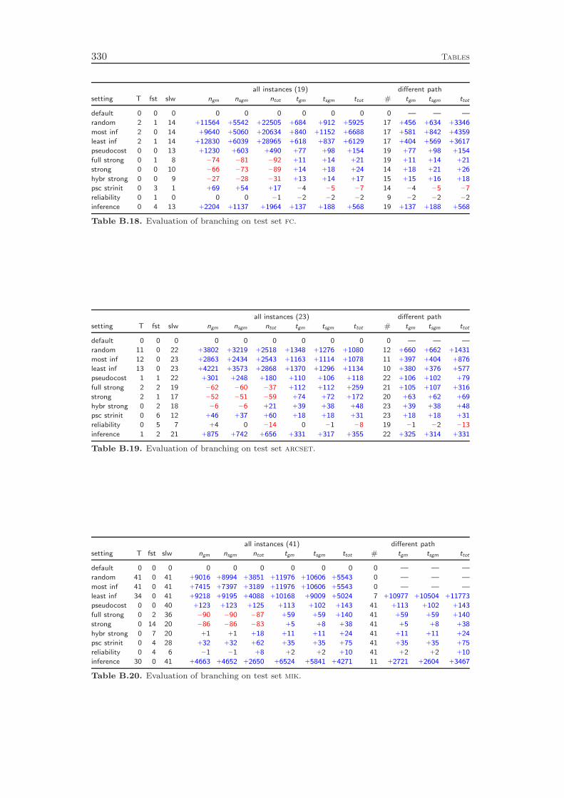
330 Tables
all instances (19) different path
setting T fst slw ngm nsgm ntot tgm tsgm ttot # tgm tsgm ttot
default 0 0 0 0 0 0 0 0 0 0 — — —
random 2 1 14 +11564 +5542 +22505 +684 +912 +5925 17 +456 +634 +3346
most inf 2 0 14 +9640 +5060 +20634 +840 +1152 +6688 17 +581 +842 +4359
least inf 2 1 14 +12830 +6039 +28965 +618 +837 +6129 17 +404 +569 +3617
pseudocost 0 0 13 +1230 +603 +490 +77 +98 +154 19 +77 +98 +154
full strong 0 1 8 −74 −81 −92 +11 +14 +21 19 +11 +14 +21
strong 0 0 10 −66 −73 −89 +14 +18 +24 14 +18 +21 +26
hybr strong 0 0 9 −27 −28 −31 +13 +14 +17 15 +15 +16 +18
psc strinit 0 3 1 +69 +54 +17 −4 −5 −7 14 −4 −5 −7
reliability 0 1 0 0 0 −1 −2 −2 −2 9 −2 −2 −2
inference 0 4 13 +2204 +1137 +1964 +137 +188 +568 19 +137 +188 +568
Table B.18. Evaluation of branching on test set fc.
all instances (23) different path
setting T fst slw ngm nsgm ntot tgm tsgm ttot # tgm tsgm ttot
default 0 0 0 0 0 0 0 0 0 0 — — —
random 11 0 22 +3802 +3219 +2518 +1348 +1276 +1080 12 +660 +662 +1431
most inf 12 0 23 +2863 +2434 +2543 +1163 +1114 +1078 11 +397 +404 +876
least inf 13 0 23 +4221 +3573 +2868 +1370 +1296 +1134 10 +380 +376 +577
pseudocost 1 1 22 +301 +248 +180 +110 +106 +118 22 +106 +102 +79
full strong 2 2 19 −62 −60 −37 +112 +112 +259 21 +105 +107 +316
strong 2 1 17 −52 −51 −59 +74 +72 +172 20 +63 +62 +69
hybr strong 0 2 18 −6 −6 +21 +39 +38 +48 23 +39 +38 +48
psc strinit 0 6 12 +46 +37 +60 +18 +18 +31 23 +18 +18 +31
reliability 0 5 7 +4 0 −14 0 −1 −8 19 −1 −2 −13
inference 1 2 21 +875 +742 +656 +331 +317 +355 22 +325 +314 +331
Table B.19. Evaluation of branching on test set arcset.
all instances (41) different path
setting T fst slw ngm nsgm ntot tgm tsgm ttot # tgm tsgm ttot
default 0 0 0 0 0 0 0 0 0 0 — — —
random 41 0 41 +9016 +8994 +3851 +11976 +10606 +5543 0 — — —
most inf 41 0 41 +7415 +7397 +3189 +11976 +10606 +5543 0 — — —
least inf 34 0 41 +9218 +9195 +4088 +10168 +9009 +5024 7 +10977 +10504 +11773
pseudocost 0 0 40 +123 +123 +125 +113 +102 +143 41 +113 +102 +143
full strong 0 2 36 −90 −90 −87 +59 +59 +140 41 +59 +59 +140
strong 0 14 20 −86 −86 −83 +5 +8 +38 41 +5 +8 +38
hybr strong 0 7 20 +1 +1 +18 +11 +11 +24 41 +11 +11 +24
psc strinit 0 4 28 +32 +32 +62 +35 +35 +75 41 +35 +35 +75
reliability 0 4 6 −1 −1 +8 +2 +2 +10 41 +2 +2 +10
inference 30 0 41 +4663 +4652 +2650 +6524 +5841 +4271 11 +2721 +2604 +3467
Table B.20. Evaluation of branching on test set mik.

Tables 331
Branching Score Function
all instances (30) different path equal path
setting T fst slw ngm nsgm ntot tgm tsgm ttot # tgm tsgm ttot # tgm tsgm ttot
default 1 0 0 0 0 0 0 0 0 0 — — — 29 0 0 0
min (µ = 0) 2 1 12 +22 +24 −5 +26 +26 +40 24 +32 +32 +66 4 +1 +1 0
weighted (µ = 16
) 2 4 9 +27 +21 +2 +12 +12 +23 24 +10 +10 +5 4 −1 −1 −1
weighted (µ = 13
) 3 4 10 +58 +46 +24 +26 +28 +61 23 +21 +23 +35 4 −1 −1 −1
avg (µ = 12
) 2 0 14 +88 +73 +9 +29 +30 +50 24 +29 +29 +42 4 −1 −1 −2
max (µ = 1) 4 1 16 +109 +92 +41 +53 +53 +80 22 +57 +58 +92 4 −1 −1 −1
Table B.21. Evaluation of branching score functions on test set miplib.
all instances (37) different path equal path
setting T fst slw ngm nsgm ntot tgm tsgm ttot # tgm tsgm ttot # tgm tsgm ttot
default 2 0 0 0 0 0 0 0 0 0 — — — 35 0 0 0
min (µ = 0) 3 7 19 +23 +25 +4 +26 +25 +30 31 +31 +31 +51 2 +1 +1 +1
weighted (µ = 16
) 5 8 13 +49 +48 +7 +21 +20 +43 30 +11 +10 +8 2 −1 −1 −1
weighted (µ = 13
) 4 12 12 +47 +53 +6 +26 +27 +42 30 +23 +25 +40 2 −3 −3 −2
avg (µ = 12
) 5 7 20 +119 +102 +27 +50 +49 +66 30 +45 +44 +62 2 +1 +1 +1
max (µ = 1) 7 5 23 +220 +199 +94 +113 +113 +135 28 +87 +88 +155 2 +1 +1 +1
Table B.22. Evaluation of branching score functions on test set coral.
all instances (35) different path equal path
setting T fst slw ngm nsgm ntot tgm tsgm ttot # tgm tsgm ttot # tgm tsgm ttot
default 6 0 0 0 0 0 0 0 0 0 — — — 29 0 0 0
min (µ = 0) 8 4 11 +28 +19 −13 +18 +18 +15 18 +26 +27 +34 8 0 0 0
weighted (µ = 16
) 7 5 10 +36 +26 −11 +10 +10 +6 19 +10 +8 −8 8 0 0 0
weighted (µ = 13
) 8 3 12 +80 +69 +5 +37 +36 +25 19 +52 +50 +62 7 +2 +2 +3
avg (µ = 12
) 10 4 13 +67 +68 +22 +36 +35 +33 20 +39 +37 +47 5 +1 +1 +1
max (µ = 1) 11 2 16 +106 +97 +17 +59 +58 +48 19 +74 +73 +94 5 +2 +2 +3
Table B.23. Evaluation of branching score functions on test set milp.
all instances (7) different path equal path
setting T fst slw ngm nsgm ntot tgm tsgm ttot # tgm tsgm ttot # tgm tsgm ttot
default 0 0 0 0 0 0 0 0 0 0 — — — 7 0 0 0
min (µ = 0) 0 1 4 +10 +12 +67 +26 +34 +73 6 +31 +38 +73 1 0 0 0
weighted (µ = 16
) 0 3 2 −13 −13 −48 −10 −19 −52 6 −11 −21 −52 1 0 0 0
weighted (µ = 13
) 0 2 3 +14 +15 −23 +18 −1 −30 6 +21 −1 −30 1 0 0 0
avg (µ = 12
) 0 3 2 +2 +2 −9 0 −9 −22 6 0 −10 −22 1 0 0 0
max (µ = 1) 0 1 4 +115 +116 +194 +113 +115 +172 6 +141 +135 +172 1 0 0 0
Table B.24. Evaluation of branching score functions on test set enlight.
all instances (25) different path equal path
setting T fst slw ngm nsgm ntot tgm tsgm ttot # tgm tsgm ttot # tgm tsgm ttot
default 1 0 0 0 0 0 0 0 0 0 — — — 24 0 0 0
min (µ = 0) 3 3 13 +70 +85 +108 +78 +88 +161 17 +79 +86 +188 5 0 0 0
weighted (µ = 16
) 1 3 12 +117 +104 +53 +76 +66 +48 19 +111 +90 +111 5 0 0 0
weighted (µ = 13
) 2 2 13 +94 +96 +92 +79 +85 +116 18 +73 +71 +139 5 0 0 0
avg (µ = 12
) 2 3 14 +195 +165 +86 +116 +101 +108 19 +116 +88 +121 4 0 0 0
max (µ = 1) 3 1 16 +499 +357 +135 +239 +187 +185 19 +256 +183 +250 3 0 0 0
Table B.25. Evaluation of branching score functions on test set alu.
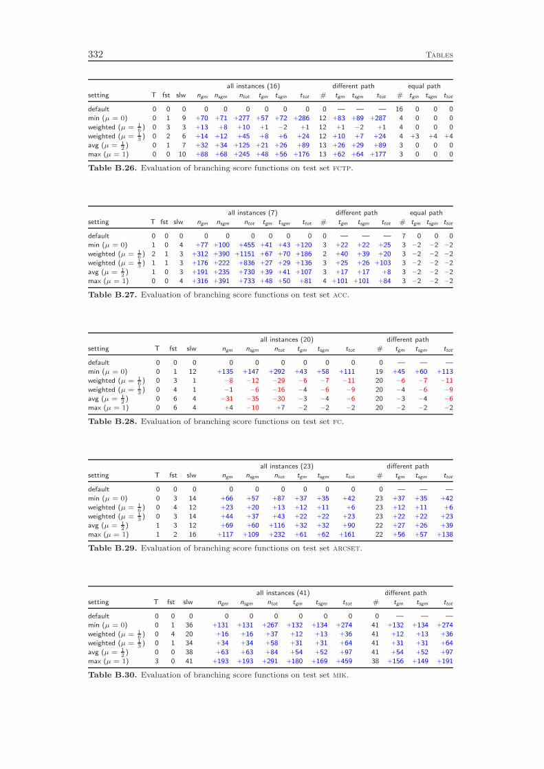
332 Tables
all instances (16) different path equal path
setting T fst slw ngm nsgm ntot tgm tsgm ttot # tgm tsgm ttot # tgm tsgm ttot
default 0 0 0 0 0 0 0 0 0 0 — — — 16 0 0 0
min (µ = 0) 0 1 9 +70 +71 +277 +57 +72 +286 12 +83 +89 +287 4 0 0 0
weighted (µ = 16
) 0 3 3 +13 +8 +10 +1 −2 +1 12 +1 −2 +1 4 0 0 0
weighted (µ = 13
) 0 2 6 +14 +12 +45 +8 +6 +24 12 +10 +7 +24 4 +3 +4 +4
avg (µ = 12
) 0 1 7 +32 +34 +125 +21 +26 +89 13 +26 +29 +89 3 0 0 0
max (µ = 1) 0 0 10 +88 +68 +245 +48 +56 +176 13 +62 +64 +177 3 0 0 0
Table B.26. Evaluation of branching score functions on test set fctp.
all instances (7) different path equal path
setting T fst slw ngm nsgm ntot tgm tsgm ttot # tgm tsgm ttot # tgm tsgm ttot
default 0 0 0 0 0 0 0 0 0 0 — — — 7 0 0 0
min (µ = 0) 1 0 4 +77 +100 +455 +41 +43 +120 3 +22 +22 +25 3 −2 −2 −2
weighted (µ = 16
) 2 1 3 +312 +390 +1151 +67 +70 +186 2 +40 +39 +20 3 −2 −2 −2
weighted (µ = 13
) 1 1 3 +176 +222 +836 +27 +29 +136 3 +25 +26 +103 3 −2 −2 −2
avg (µ = 12
) 1 0 3 +191 +235 +730 +39 +41 +107 3 +17 +17 +8 3 −2 −2 −2
max (µ = 1) 0 0 4 +316 +391 +733 +48 +50 +81 4 +101 +101 +84 3 −2 −2 −2
Table B.27. Evaluation of branching score functions on test set acc.
all instances (20) different path
setting T fst slw ngm nsgm ntot tgm tsgm ttot # tgm tsgm ttot
default 0 0 0 0 0 0 0 0 0 0 — — —
min (µ = 0) 0 1 12 +135 +147 +292 +43 +58 +111 19 +45 +60 +113
weighted (µ = 16
) 0 3 1 −8 −12 −29 −6 −7 −11 20 −6 −7 −11
weighted (µ = 13
) 0 4 1 −1 −6 −16 −4 −6 −9 20 −4 −6 −9
avg (µ = 12
) 0 6 4 −31 −35 −30 −3 −4 −6 20 −3 −4 −6
max (µ = 1) 0 6 4 +4 −10 +7 −2 −2 −2 20 −2 −2 −2
Table B.28. Evaluation of branching score functions on test set fc.
all instances (23) different path
setting T fst slw ngm nsgm ntot tgm tsgm ttot # tgm tsgm ttot
default 0 0 0 0 0 0 0 0 0 0 — — —
min (µ = 0) 0 3 14 +66 +57 +87 +37 +35 +42 23 +37 +35 +42
weighted (µ = 16
) 0 4 12 +23 +20 +13 +12 +11 +6 23 +12 +11 +6
weighted (µ = 13
) 0 3 14 +44 +37 +43 +22 +22 +23 23 +22 +22 +23
avg (µ = 12
) 1 3 12 +69 +60 +116 +32 +32 +90 22 +27 +26 +39
max (µ = 1) 1 2 16 +117 +109 +232 +61 +62 +161 22 +56 +57 +138
Table B.29. Evaluation of branching score functions on test set arcset.
all instances (41) different path
setting T fst slw ngm nsgm ntot tgm tsgm ttot # tgm tsgm ttot
default 0 0 0 0 0 0 0 0 0 0 — — —
min (µ = 0) 0 1 36 +131 +131 +267 +132 +134 +274 41 +132 +134 +274
weighted (µ = 16
) 0 4 20 +16 +16 +37 +12 +13 +36 41 +12 +13 +36
weighted (µ = 13
) 0 1 34 +34 +34 +58 +31 +31 +64 41 +31 +31 +64
avg (µ = 12
) 0 0 38 +63 +63 +84 +54 +52 +97 41 +54 +52 +97
max (µ = 1) 3 0 41 +193 +193 +291 +180 +169 +459 38 +156 +149 +191
Table B.30. Evaluation of branching score functions on test set mik.

Tables 333
Node Selection
all instances (30) different path equal path
setting T fst slw ngm nsgm ntot tgm tsgm ttot # tgm tsgm ttot # tgm tsgm ttot
default 1 0 0 0 0 0 0 0 0 0 — — — 29 0 0 0
dfs 2 5 8 +60 +64 +81 +22 +22 +36 18 +26 +22 +4 9 −2 −2 −2
bfs 1 3 15 −24 −18 −15 +30 +28 +25 25 +37 +34 +37 4 −2 −2 −2
bfs/plunge 1 2 6 +5 +3 +24 +4 +3 +4 20 +7 +5 +7 9 0 0 0
estimate 1 3 13 −18 −15 +24 +15 +14 +12 23 +20 +18 +18 6 0 0 −1
estim/plunge 1 6 3 −3 −3 +15 −3 −3 −10 18 −6 −5 −15 11 0 0 0
hybrid 2 3 7 +7 +7 +26 +8 +8 +18 18 +5 +4 −10 10 −2 −1 −2
Table B.31. Evaluation of node selection on test set miplib.
all instances (38) different path equal path
setting T fst slw ngm nsgm ntot tgm tsgm ttot # tgm tsgm ttot # tgm tsgm ttot
default 3 0 0 0 0 0 0 0 0 0 — — — 35 0 0 0
dfs 7 13 15 +145 +143 +38 +51 +49 +69 28 +11 +12 +31 3 +1 +1 +1
bfs 5 6 20 −41 −28 −1 +37 +38 +46 30 +31 +33 +52 3 +3 +3 +4
bfs/plunge 2 6 18 −1 0 −12 +2 +2 −10 30 +15 +15 +10 5 +2 +2 +2
estimate 4 9 19 −23 −9 −5 +19 +19 +17 30 +24 +25 +29 3 0 0 0
estim/plunge 2 8 10 +3 +3 −9 −3 −3 −11 30 +1 +1 +4 5 +2 +2 +2
hybrid 2 7 10 −9 −9 0 −5 −5 −10 30 +4 +4 +10 5 +3 +2 +2
Table B.32. Evaluation of node selection on test set coral.
all instances (35) different path equal path
setting T fst slw ngm nsgm ntot tgm tsgm ttot # tgm tsgm ttot # tgm tsgm ttot
default 6 0 0 0 0 0 0 0 0 0 — — — 29 0 0 0
dfs 6 5 13 +57 +41 +8 +12 +12 +7 18 +13 +13 +10 9 +1 +1 +1
bfs 6 5 12 −24 −12 −6 +20 +20 +13 20 +39 +38 +57 8 0 0 −1
bfs/plunge 4 4 8 +3 +2 +9 +2 +1 −4 17 +8 +8 +8 11 +1 +1 +2
estimate 5 6 12 −19 −9 +9 +9 +8 +3 20 +17 +15 +16 8 −1 0 −1
estim/plunge 4 3 7 +9 +9 +18 +5 +5 +2 16 +11 +11 +14 13 +3 +2 +2
hybrid 6 2 8 +9 +8 +28 +4 +3 0 18 +6 +5 −1 11 +2 +2 +3
Table B.33. Evaluation of node selection on test set milp.
all instances (7) different path equal path
setting T fst slw ngm nsgm ntot tgm tsgm ttot # tgm tsgm ttot # tgm tsgm ttot
default 0 0 0 0 0 0 0 0 0 0 — — — 7 0 0 0
dfs 0 1 4 +109 +109 +51 +73 +53 +9 6 +90 +61 +9 1 0 0 0
bfs 0 1 4 +14 +16 +61 +78 +74 +136 6 +95 +86 +136 1 0 0 0
bfs/plunge 1 1 4 +35 +36 +200 +42 +53 +173 5 +39 +57 +275 1 0 0 0
estimate 0 2 3 +1 +2 −52 +24 0 −49 6 +28 0 −49 1 0 0 0
estim/plunge 0 2 1 +7 +7 −11 −5 −11 −29 6 −5 −12 −29 1 0 0 0
hybrid 0 2 3 +12 +13 +113 +20 +25 +108 6 +24 +28 +108 1 0 0 0
Table B.34. Evaluation of node selection on test set enlight.
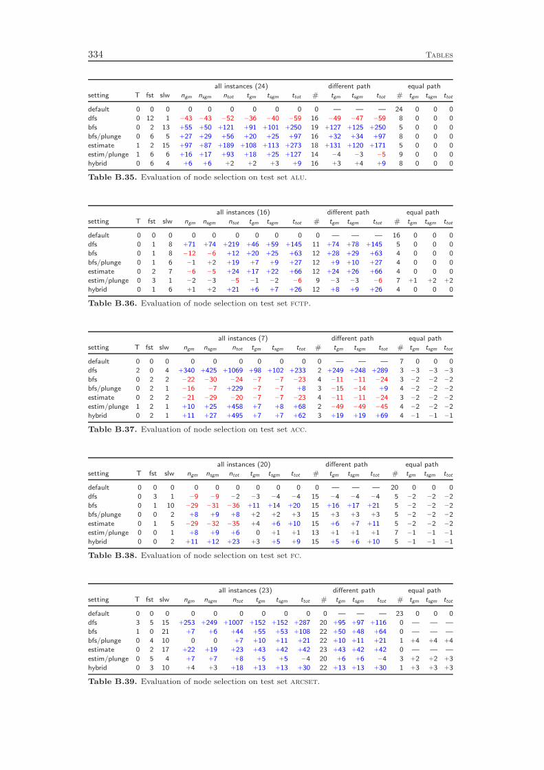
334 Tables
all instances (24) different path equal path
setting T fst slw ngm nsgm ntot tgm tsgm ttot # tgm tsgm ttot # tgm tsgm ttot
default 0 0 0 0 0 0 0 0 0 0 — — — 24 0 0 0
dfs 0 12 1 −43 −43 −52 −36 −40 −59 16 −49 −47 −59 8 0 0 0
bfs 0 2 13 +55 +50 +121 +91 +101 +250 19 +127 +125 +250 5 0 0 0
bfs/plunge 0 6 5 +27 +29 +56 +20 +25 +97 16 +32 +34 +97 8 0 0 0
estimate 1 2 15 +97 +87 +189 +108 +113 +273 18 +131 +120 +171 5 0 0 0
estim/plunge 1 6 6 +16 +17 +93 +18 +25 +127 14 −4 −3 −5 9 0 0 0
hybrid 0 6 4 +6 +6 +2 +2 +3 +9 16 +3 +4 +9 8 0 0 0
Table B.35. Evaluation of node selection on test set alu.
all instances (16) different path equal path
setting T fst slw ngm nsgm ntot tgm tsgm ttot # tgm tsgm ttot # tgm tsgm ttot
default 0 0 0 0 0 0 0 0 0 0 — — — 16 0 0 0
dfs 0 1 8 +71 +74 +219 +46 +59 +145 11 +74 +78 +145 5 0 0 0
bfs 0 1 8 −12 −6 +12 +20 +25 +63 12 +28 +29 +63 4 0 0 0
bfs/plunge 0 1 6 −1 +2 +19 +7 +9 +27 12 +9 +10 +27 4 0 0 0
estimate 0 2 7 −6 −5 +24 +17 +22 +66 12 +24 +26 +66 4 0 0 0
estim/plunge 0 3 1 −2 −3 −5 −1 −2 −6 9 −3 −3 −6 7 +1 +2 +2
hybrid 0 1 6 +1 +2 +21 +6 +7 +26 12 +8 +9 +26 4 0 0 0
Table B.36. Evaluation of node selection on test set fctp.
all instances (7) different path equal path
setting T fst slw ngm nsgm ntot tgm tsgm ttot # tgm tsgm ttot # tgm tsgm ttot
default 0 0 0 0 0 0 0 0 0 0 — — — 7 0 0 0
dfs 2 0 4 +340 +425 +1069 +98 +102 +233 2 +249 +248 +289 3 −3 −3 −3
bfs 0 2 2 −22 −30 −24 −7 −7 −23 4 −11 −11 −24 3 −2 −2 −2
bfs/plunge 0 2 1 −16 −7 +229 −7 −7 +8 3 −15 −14 +9 4 −2 −2 −2
estimate 0 2 2 −21 −29 −20 −7 −7 −23 4 −11 −11 −24 3 −2 −2 −2
estim/plunge 1 2 1 +10 +25 +458 +7 +8 +68 2 −49 −49 −45 4 −2 −2 −2
hybrid 0 2 1 +11 +27 +495 +7 +7 +62 3 +19 +19 +69 4 −1 −1 −1
Table B.37. Evaluation of node selection on test set acc.
all instances (20) different path equal path
setting T fst slw ngm nsgm ntot tgm tsgm ttot # tgm tsgm ttot # tgm tsgm ttot
default 0 0 0 0 0 0 0 0 0 0 — — — 20 0 0 0
dfs 0 3 1 −9 −9 −2 −3 −4 −4 15 −4 −4 −4 5 −2 −2 −2
bfs 0 1 10 −29 −31 −36 +11 +14 +20 15 +16 +17 +21 5 −2 −2 −2
bfs/plunge 0 0 2 +8 +9 +8 +2 +2 +3 15 +3 +3 +3 5 −2 −2 −2
estimate 0 1 5 −29 −32 −35 +4 +6 +10 15 +6 +7 +11 5 −2 −2 −2
estim/plunge 0 0 1 +8 +9 +6 0 +1 +1 13 +1 +1 +1 7 −1 −1 −1
hybrid 0 0 2 +11 +12 +23 +3 +5 +9 15 +5 +6 +10 5 −1 −1 −1
Table B.38. Evaluation of node selection on test set fc.
all instances (23) different path equal path
setting T fst slw ngm nsgm ntot tgm tsgm ttot # tgm tsgm ttot # tgm tsgm ttot
default 0 0 0 0 0 0 0 0 0 0 — — — 23 0 0 0
dfs 3 5 15 +253 +249 +1007 +152 +152 +287 20 +95 +97 +116 0 — — —
bfs 1 0 21 +7 +6 +44 +55 +53 +108 22 +50 +48 +64 0 — — —
bfs/plunge 0 4 10 0 0 +7 +10 +11 +21 22 +10 +11 +21 1 +4 +4 +4
estimate 0 2 17 +22 +19 +23 +43 +42 +42 23 +43 +42 +42 0 — — —
estim/plunge 0 5 4 +7 +7 +8 +5 +5 −4 20 +6 +6 −4 3 +2 +2 +3
hybrid 0 3 10 +4 +3 +18 +13 +13 +30 22 +13 +13 +30 1 +3 +3 +3
Table B.39. Evaluation of node selection on test set arcset.
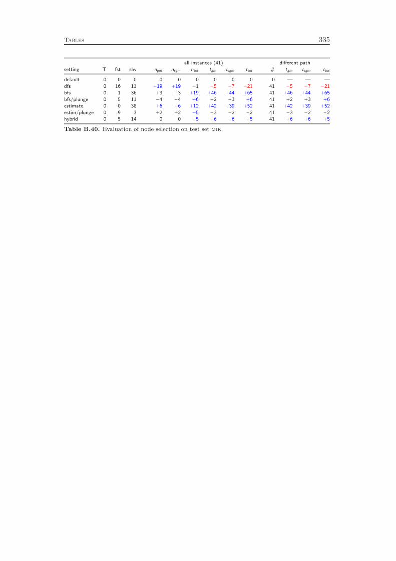
Tables 335
all instances (41) different path
setting T fst slw ngm nsgm ntot tgm tsgm ttot # tgm tsgm ttot
default 0 0 0 0 0 0 0 0 0 0 — — —
dfs 0 16 11 +19 +19 −1 −5 −7 −21 41 −5 −7 −21
bfs 0 1 36 +3 +3 +19 +46 +44 +65 41 +46 +44 +65
bfs/plunge 0 5 11 −4 −4 +6 +2 +3 +6 41 +2 +3 +6
estimate 0 0 38 +6 +6 +12 +42 +39 +52 41 +42 +39 +52
estim/plunge 0 9 3 +2 +2 +5 −3 −2 −2 41 −3 −2 −2
hybrid 0 5 14 0 0 +5 +6 +6 +5 41 +6 +6 +5
Table B.40. Evaluation of node selection on test set mik.

336 Tables
Child Selection
all instances (30) different path equal path
setting T fst slw ngm nsgm ntot tgm tsgm ttot # tgm tsgm ttot # tgm tsgm ttot
default 1 0 0 0 0 0 0 0 0 0 — — — 29 0 0 0
down 1 2 11 +20 +18 +5 +22 +23 +27 22 +31 +32 +40 7 −1 −1 −1
up 1 5 4 +3 −1 −6 0 0 +2 23 0 0 +3 6 −1 −1 −2
pseudocost 2 6 7 −11 −8 −15 +11 +12 +20 22 +13 +15 +24 6 −2 −2 −2
LP value 1 9 9 +5 +1 −20 +7 +7 +3 22 +10 +10 +5 7 −1 0 −1
root LP value 1 3 6 +2 −2 −6 +1 0 +1 25 +2 0 +1 4 0 0 0
inference 1 4 4 −5 −4 +6 +4 +4 +1 19 +6 +6 +2 10 +1 0 0
Table B.41. Evaluation of child selection on test set miplib.
all instances (38) different path equal path
setting T fst slw ngm nsgm ntot tgm tsgm ttot # tgm tsgm ttot # tgm tsgm ttot
default 3 0 0 0 0 0 0 0 0 0 — — — 35 0 0 0
down 3 10 13 +11 +14 +5 +11 +10 +12 30 +6 +4 +10 4 0 0 0
up 3 14 4 −27 −19 +65 −12 −11 +3 31 −14 −13 +7 4 +1 +1 +1
pseudocost 4 14 9 −7 −1 +20 +5 +6 +17 30 −4 −3 −2 3 −2 −2 −2
LP value 2 11 10 −13 −9 +5 −2 −2 −5 32 +1 +1 +10 3 −1 −1 0
root LP value 4 15 5 −19 −14 −11 −6 −5 +9 31 −10 −9 +1 3 0 0 0
inference 3 13 5 +3 +1 −7 −3 −4 −4 30 −4 −5 −8 5 −1 −1 −1
Table B.42. Evaluation of child selection on test set coral.
all instances (35) different path equal path
setting T fst slw ngm nsgm ntot tgm tsgm ttot # tgm tsgm ttot # tgm tsgm ttot
default 6 0 0 0 0 0 0 0 0 0 — — — 29 0 0 0
down 5 4 10 +7 +8 −6 +15 +14 +11 20 +31 +30 +45 9 +1 +1 +1
up 4 8 3 −11 −9 +5 −5 −5 0 19 −9 −9 +10 10 +3 +2 +2
pseudocost 5 8 10 +7 +10 −9 +11 +10 +7 20 +24 +23 +50 8 +1 +1 +1
LP value 5 5 12 +11 +15 −4 +13 +12 +14 21 +23 +22 +48 8 0 +1 +1
root LP value 5 9 4 −10 −9 −1 −8 −8 −5 20 −13 −13 −12 9 0 +1 0
inference 3 5 6 −15 −12 +3 −4 −5 −8 17 −6 −7 −10 12 +1 +1 +2
Table B.43. Evaluation of child selection on test set milp.
all instances (7) different path equal path
setting T fst slw ngm nsgm ntot tgm tsgm ttot # tgm tsgm ttot # tgm tsgm ttot
default 0 0 0 0 0 0 0 0 0 0 — — — 7 0 0 0
down 0 1 3 −5 −4 +16 +2 −1 +11 6 +3 −1 +11 1 0 0 0
up 0 1 3 +20 +20 −12 +17 +3 −16 6 +20 +4 −16 1 0 0 0
pseudocost 0 2 2 −3 −3 +34 +1 −2 +22 6 +1 −2 +22 1 0 0 0
LP value 0 3 1 −9 −9 −17 −9 −11 −28 6 −10 −12 −28 1 0 0 0
root LP value 0 2 1 −3 −3 −11 −5 −8 −16 6 −6 −8 −16 1 0 0 0
inference 0 2 3 +7 +7 +27 +10 +3 +22 6 +11 +4 +22 1 0 0 0
Table B.44. Evaluation of child selection on test set enlight.
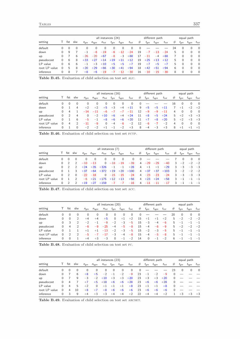
Tables 337
all instances (24) different path equal path
setting T fst slw ngm nsgm ntot tgm tsgm ttot # tgm tsgm ttot # tgm tsgm ttot
default 0 0 0 0 0 0 0 0 0 0 — — — 24 0 0 0
down 0 9 7 −1 −6 −19 −6 −12 −24 19 −7 −13 −24 5 0 0 0
up 0 7 6 −26 −20 +67 −8 −3 +88 17 −11 −4 +88 7 0 0 0
pseudocost 0 6 8 +33 +27 +14 +19 +11 +12 19 +25 +13 +12 5 0 0 0
LP value 0 6 6 −1 +3 +10 +5 +5 +7 19 +7 +5 +7 5 0 0 0
root LP value 0 5 8 +20 +29 +66 +30 +41 +94 18 +42 +51 +94 6 0 0 0
inference 0 8 7 +8 +6 −19 −7 −12 −30 16 −10 −15 −30 8 0 0 0
Table B.45. Evaluation of child selection on test set alu.
all instances (16) different path equal path
setting T fst slw ngm nsgm ntot tgm tsgm ttot # tgm tsgm ttot # tgm tsgm ttot
default 0 0 0 0 0 0 0 0 0 0 — — — 16 0 0 0
down 0 1 4 +2 +2 +5 +3 +4 +11 9 +5 +5 +11 7 +1 +2 +2
up 0 4 1 −14 −11 −6 −7 −7 −11 12 −9 −9 −11 4 0 0 0
pseudocost 0 2 4 0 −2 +10 +6 +4 +24 11 +8 +5 +24 5 +2 +3 +3
LP value 0 1 6 −5 −1 +8 +6 +6 +20 11 +7 +8 +20 5 +2 +3 +3
root LP value 0 4 2 −11 −9 0 −4 −6 −2 12 −6 −7 −2 4 0 0 0
inference 0 1 0 −2 −2 +1 −1 −2 +3 8 −4 −3 +3 8 +1 +1 +1
Table B.46. Evaluation of child selection on test set fctp.
all instances (7) different path equal path
setting T fst slw ngm nsgm ntot tgm tsgm ttot # tgm tsgm ttot # tgm tsgm ttot
default 0 0 0 0 0 0 0 0 0 0 — — — 7 0 0 0
down 0 2 2 −10 −13 0 −18 −19 −39 4 −29 −29 −40 3 −2 −2 −2
up 0 2 2 +24 +35 +326 −1 −1 +28 4 +1 +1 +29 3 −3 −3 −3
pseudocost 0 1 3 +37 +64 +372 +19 +20 +100 4 +37 +37 +103 3 −2 −2 −2
LP value 0 2 0 −22 −18 0 −15 −15 −24 4 −23 −23 −24 3 −3 −3 −3
root LP value 0 1 2 −6 +21 +175 +12 +13 +56 4 +23 +24 +58 3 −1 −1 −1
inference 0 2 2 +19 +27 +159 −7 −7 −16 4 −11 −11 −17 3 −1 −1 −1
Table B.47. Evaluation of child selection on test set acc.
all instances (20) different path equal path
setting T fst slw ngm nsgm ntot tgm tsgm ttot # tgm tsgm ttot # tgm tsgm ttot
default 0 0 0 0 0 0 0 0 0 0 — — — 20 0 0 0
down 0 0 2 +4 +4 +5 0 +1 +2 15 +1 +1 +2 5 −2 −2 −2
up 0 3 2 −2 −1 −9 −2 −3 −5 15 −3 −4 −6 5 −1 −1 −1
pseudocost 0 4 2 −6 −9 −25 −4 −5 −8 15 −4 −6 −9 5 −2 −2 −2
LP value 0 1 1 +1 +1 −13 −2 −3 −5 15 −2 −3 −5 5 −1 −1 −1
root LP value 0 2 2 −5 −7 −17 −3 −4 −8 15 −4 −5 −8 5 −1 −1 −1
inference 0 0 1 +4 +3 −3 0 −1 −2 14 0 −1 −2 6 −1 −1 −1
Table B.48. Evaluation of child selection on test set fc.
all instances (23) different path equal path
setting T fst slw ngm nsgm ntot tgm tsgm ttot # tgm tsgm ttot # tgm tsgm ttot
default 0 0 0 0 0 0 0 0 0 0 — — — 23 0 0 0
down 0 7 6 +8 +5 −2 −1 −2 −9 23 −1 −2 −9 0 — — —
up 0 7 9 −3 −2 +10 +3 +3 +20 23 +3 +3 +20 0 — — —
pseudocost 0 4 7 +7 +5 +18 +6 +6 +28 23 +6 +6 +28 0 — — —
LP value 0 4 5 +2 0 +1 +1 +1 +8 23 +1 +1 +8 0 — — —
root LP value 0 4 10 +8 +7 +8 +6 +6 +6 23 +6 +6 +6 0 — — —
inference 0 3 9 +4 +3 +3 +4 +4 +2 22 +4 +4 +2 1 +3 +3 +3
Table B.49. Evaluation of child selection on test set arcset.

338 Tables
all instances (41) different path
setting T fst slw ngm nsgm ntot tgm tsgm ttot # tgm tsgm ttot
default 0 0 0 0 0 0 0 0 0 0 — — —
down 0 24 9 +13 +13 +4 −9 −8 −15 41 −9 −8 −15
up 0 6 18 −5 −5 −4 +8 +8 +9 41 +8 +8 +9
pseudocost 0 4 23 +12 +12 +18 +19 +19 +34 41 +19 +19 +34
LP value 0 1 24 +20 +20 +19 +17 +17 +24 41 +17 +17 +24
root LP value 0 11 14 +12 +12 +25 +1 +2 +15 41 +1 +2 +15
inference 0 9 3 −5 −5 −3 −1 −1 +2 41 −1 −1 +2
Table B.50. Evaluation of child selection on test set mik.
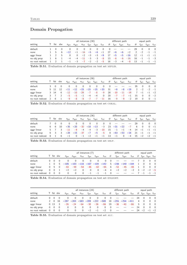
Tables 339
Domain Propagation
all instances (30) different path equal path
setting T fst slw ngm nsgm ntot tgm tsgm ttot # tgm tsgm ttot # tgm tsgm ttot
default 1 0 0 0 0 0 0 0 0 0 — — — 29 0 0 0
none 1 5 6 +12 +1 −16 +5 +6 +1 27 +6 +6 +2 2 −2 −1 −1
aggr linear 1 2 5 0 0 +2 +3 +3 +9 17 +5 +5 +16 12 +1 +1 +1
no obj prop 1 6 1 −4 −4 −11 −3 −3 −8 13 −6 −6 −16 16 −1 −1 −3
no root redcost 1 2 1 −1 −3 −7 −2 −2 −5 16 −3 −4 −8 13 −1 −1 −1
Table B.51. Evaluation of domain propagation on test set miplib.
all instances (38) different path equal path
setting T fst slw ngm nsgm ntot tgm tsgm ttot # tgm tsgm ttot # tgm tsgm ttot
default 3 0 0 0 0 0 0 0 0 0 — — — 35 0 0 0
none 5 11 12 +11 +12 +15 +15 +15 +33 31 +8 +8 +19 2 −2 −2 −1
aggr linear 3 14 6 −12 −10 −29 −7 −8 −9 28 −10 −11 −19 7 +1 +1 +2
no obj prop 3 7 2 −5 −5 −1 −4 −4 0 20 −7 −7 +1 15 0 0 −2
no root redcost 2 6 1 −9 −8 −8 −7 −7 −11 16 −9 −9 −2 19 0 0 −1
Table B.52. Evaluation of domain propagation on test set coral.
all instances (36) different path equal path
setting T fst slw ngm nsgm ntot tgm tsgm ttot # tgm tsgm ttot # tgm tsgm ttot
default 7 0 0 0 0 0 0 0 0 0 — — — 29 0 0 0
none 6 6 10 +35 +20 −32 +18 +13 −3 23 +31 +22 −7 6 0 0 +1
aggr linear 5 7 3 −11 −9 −4 −4 −3 −10 15 −1 +1 −4 14 +1 +1 +1
no obj prop 6 3 3 +28 +15 −37 +7 +5 −5 8 +63 +53 +18 21 +1 +1 +1
no root redcost 8 1 6 +1 0 −1 +2 +1 +1 13 +1 0 −4 15 +2 +2 +1
Table B.53. Evaluation of domain propagation on test set milp.
all instances (7) different path equal path
setting T fst slw ngm nsgm ntot tgm tsgm ttot # tgm tsgm ttot # tgm tsgm ttot
default 0 0 0 0 0 0 0 0 0 0 — — — 7 0 0 0
none 1 0 5 +185 +183 +118 +167 +104 +142 5 +238 +140 +184 1 0 0 0
aggr linear 0 5 0 −61 −59 −54 −46 −42 −65 6 −51 −45 −65 1 0 0 0
no obj prop 0 0 1 +2 +2 0 0 0 −4 4 +2 +2 −2 3 −2 −2 −5
no root redcost 0 0 0 0 0 0 −1 −1 −1 0 — — — 7 −1 −1 −1
Table B.54. Evaluation of domain propagation on test set enlight.
all instances (24) different path equal path
setting T fst slw ngm nsgm ntot tgm tsgm ttot # tgm tsgm ttot # tgm tsgm ttot
default 0 0 0 0 0 0 0 0 0 0 — — — 24 0 0 0
none 2 0 16 +287 +283 +583 +209 +222 +508 18 +255 +254 +411 4 0 0 0
aggr linear 0 13 3 −26 −24 −64 −30 −36 −66 19 −36 −40 −66 5 0 0 0
no obj prop 0 0 0 0 0 0 0 0 0 0 — — — 24 0 0 0
no root redcost 0 0 0 0 0 0 +2 +1 +2 0 — — — 24 +2 +1 +2
Table B.55. Evaluation of domain propagation on test set alu.
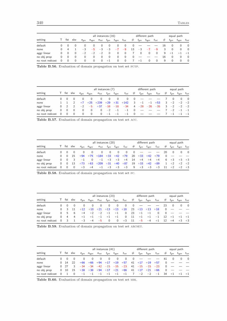
340 Tables
all instances (16) different path equal path
setting T fst slw ngm nsgm ntot tgm tsgm ttot # tgm tsgm ttot # tgm tsgm ttot
default 0 0 0 0 0 0 0 0 0 0 — — — 16 0 0 0
none 0 4 1 −3 −5 −3 −3 −7 −9 13 −3 −7 −9 3 0 0 0
aggr linear 0 0 0 −2 −2 −2 0 0 0 7 0 0 0 9 +1 +1 +1
no obj prop 0 0 0 0 0 0 0 0 0 0 — — — 16 0 0 0
no root redcost 0 0 0 0 0 0 +1 0 0 7 +1 0 0 9 0 0 0
Table B.56. Evaluation of domain propagation on test set fctp.
all instances (7) different path equal path
setting T fst slw ngm nsgm ntot tgm tsgm ttot # tgm tsgm ttot # tgm tsgm ttot
default 0 0 0 0 0 0 0 0 0 0 — — — 7 0 0 0
none 1 1 2 +7 +25 +239 +29 +31 +142 3 −1 −1 +53 3 −2 −2 −2
aggr linear 0 2 2 −2 −5 +37 −18 −18 −34 4 −28 −28 −35 3 −2 −2 −2
no obj prop 0 0 0 0 0 0 −2 −1 −1 0 — — — 7 −2 −1 −1
no root redcost 0 0 0 0 0 0 −1 −1 −1 0 — — — 7 −1 −1 −1
Table B.57. Evaluation of domain propagation on test set acc.
all instances (20) different path equal path
setting T fst slw ngm nsgm ntot tgm tsgm ttot # tgm tsgm ttot # tgm tsgm ttot
default 0 0 0 0 0 0 0 0 0 0 — — — 20 0 0 0
none 0 0 15 +94 +75 +184 +33 +42 +79 20 +33 +42 +79 0 — — —
aggr linear 0 0 3 −1 0 −1 +3 +3 +4 14 +4 +4 +4 6 +3 +3 +3
no obj prop 0 0 13 +73 +63 +209 +31 +40 +87 19 +33 +42 +89 1 +2 +2 +2
no root redcost 0 0 0 +3 +4 +1 +3 +3 +3 9 +3 +3 +3 11 +2 +2 +3
Table B.58. Evaluation of domain propagation on test set fc.
all instances (23) different path equal path
setting T fst slw ngm nsgm ntot tgm tsgm ttot # tgm tsgm ttot # tgm tsgm ttot
default 0 0 0 0 0 0 0 0 0 0 — — — 23 0 0 0
none 0 3 11 +12 +10 +21 +13 +13 +18 23 +13 +13 +18 0 — — —
aggr linear 0 5 6 +4 +2 −2 +1 +1 0 23 +1 +1 0 0 — — —
no obj prop 0 4 4 +1 +1 −1 +1 +1 0 11 +1 +1 −1 12 +1 +1 +1
no root redcost 0 3 1 −3 −4 −5 0 0 +3 11 −5 −4 +1 12 +4 +3 +3
Table B.59. Evaluation of domain propagation on test set arcset.
all instances (41) different path equal path
setting T fst slw ngm nsgm ntot tgm tsgm ttot # tgm tsgm ttot # tgm tsgm ttot
default 0 0 0 0 0 0 0 0 0 0 — — — 41 0 0 0
none 0 14 22 +66 +66 +94 +17 +19 +57 41 +17 +19 +57 0 — — —
aggr linear 0 27 3 −34 −34 −42 −15 −15 −23 41 −15 −15 −23 0 — — —
no obj prop 0 10 15 +38 +38 +94 +17 +21 +66 41 +17 +21 +66 0 — — —
no root redcost 0 1 0 −1 −1 −1 +1 +1 +1 7 −2 −2 −1 34 +1 +1 +1
Table B.60. Evaluation of domain propagation on test set mik.

Tables 341
Cutting Plane Separation
all instances (30) different path equal path
setting T fst slw ngm nsgm ntot tgm tsgm ttot # tgm tsgm ttot # tgm tsgm ttot
default 1 0 0 0 0 0 0 0 0 0 — — — 29 0 0 0
none 6 6 22 +6599 +2958 +159 +592 +443 +220 24 +335 +273 +195 0 — — —
no knap 1 5 4 +19 +13 +1 +3 +5 +1 13 +11 +14 +3 16 −2 −2 −2
no c-MIR 1 8 6 +302 +157 0 +51 +35 +13 13 +167 +133 +89 16 −2 −1 −1
no Gom 1 17 4 +11 −1 −15 −18 −15 −19 24 −22 −19 −31 5 −5 −3 −3
no SCG 1 10 1 −10 −2 −4 −6 −5 −4 12 −13 −11 −14 17 −2 −1 −1
no flow 1 13 3 +32 +3 −16 −14 −9 −7 17 −19 −13 −31 12 −8 −6 −2
no impl 1 2 4 +36 +10 0 +1 +1 +5 9 +7 +9 +29 20 −2 −2 −2
no cliq 1 4 2 +15 +7 +1 −6 −6 +3 7 −19 −17 +19 22 −2 −2 −1
no rdcost 3 2 13 +38 +20 +28 +22 +21 +38 25 +21 +20 +30 2 −2 −2 −2
cons Gom 1 15 3 +14 +2 −15 −8 −6 −15 24 −11 −8 −25 5 +4 +3 +3
Table B.61. Evaluation of cut separation on test set miplib.
all instances (37) different path equal path
setting T fst slw ngm nsgm ntot tgm tsgm ttot # tgm tsgm ttot # tgm tsgm ttot
default 3 0 0 0 0 0 0 0 0 0 — — — 34 0 0 0
none 9 20 13 +342 +290 +164 +48 +51 +106 27 −4 −2 +45 1 −46 −46 −46
no knap 3 4 2 +15 +6 +32 +4 +4 +15 7 +24 +27 +158 27 −1 −1 0
no c-MIR 2 9 7 +16 +15 +7 +4 +3 +18 19 +44 +41 +109 15 0 0 +2
no Gom 4 14 11 +64 +54 +29 +10 +12 +31 31 +9 +11 +56 2 −2 −2 −1
no SCG 3 9 3 −1 +1 −19 −2 −3 −4 12 −2 −6 −19 21 0 0 +1
no flow 3 14 4 +15 +6 +14 −3 −1 +16 17 −1 +1 +61 17 −5 −4 −2
no impl 2 5 5 −19 −19 −20 −12 −12 −14 12 −3 −2 +13 22 +2 +2 +2
no cliq 3 3 4 +17 +12 +2 +1 +2 +3 9 +4 +7 +41 25 0 0 0
no rdcost 3 6 9 +2 +3 +29 +1 +1 +6 28 +1 +1 +15 6 +2 +2 +3
cons Gom 2 17 8 +3 0 −14 −16 −15 −17 32 −14 −13 −7 2 −1 −1 0
Table B.62. Evaluation of cut separation on test set coral.
all instances (34) different path equal path
setting T fst slw ngm nsgm ntot tgm tsgm ttot # tgm tsgm ttot # tgm tsgm ttot
default 6 0 0 0 0 0 0 0 0 0 — — — 28 0 0 0
none 6 13 14 +191 +81 −2 +8 +6 −5 25 +15 +12 +4 1 −3 −3 −3
no knap 6 0 3 +9 +9 +1 +4 +4 +2 3 +52 +52 +114 25 0 0 0
no c-MIR 6 7 7 +66 +48 +10 +20 +18 +8 12 +82 +75 +77 15 −7 −6 −5
no Gom 6 10 8 +29 +3 +6 −3 −4 −7 21 −10 −12 −25 5 +1 +1 +1
no SCG 5 7 3 +4 −5 −1 −7 −7 −9 11 −17 −19 −41 17 0 0 −1
no flow 4 7 1 −4 −3 −5 −4 −4 −8 8 −10 −9 −31 20 0 0 +1
no impl 4 5 1 −3 −4 −12 −8 −9 −16 8 −7 −8 −22 20 −1 −1 −1
no cliq 5 5 5 +22 +5 +1 −3 −7 −8 12 −11 −20 −46 16 +3 +2 +2
no rdcost 5 5 6 +5 +12 −9 +5 +5 +2 20 +9 +9 +8 8 −1 0 +1
cons Gom 4 11 8 0 −4 −9 −5 −5 −16 23 −1 0 −14 5 +3 +2 +2
Table B.63. Evaluation of cut separation on test set milp.
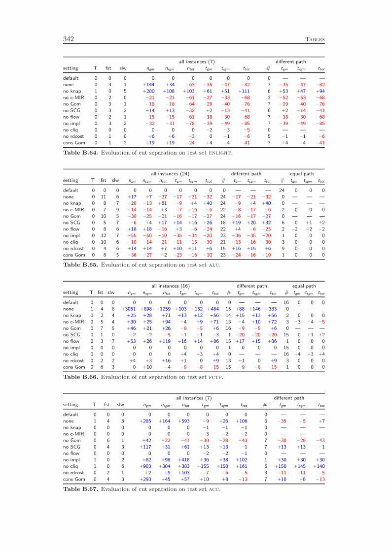
342 Tables
all instances (7) different path
setting T fst slw ngm nsgm ntot tgm tsgm ttot # tgm tsgm ttot
default 0 0 0 0 0 0 0 0 0 0 — — —
none 0 3 1 +144 +34 −63 −35 −47 −82 7 −35 −47 −82
no knap 1 0 5 +280 +108 +103 +61 +51 +111 6 +53 +47 +94
no c-MIR 0 2 0 −21 −21 −61 −27 −33 −68 3 −52 −53 −68
no Gom 0 3 1 −18 −18 −64 −29 −40 −76 7 −29 −40 −76
no SCG 0 3 2 +14 +13 −32 +2 −13 −41 6 +2 −14 −41
no flow 0 2 1 −15 −15 −61 −18 −30 −68 7 −18 −30 −68
no impl 0 3 2 −32 −31 −78 −39 −49 −85 7 −39 −49 −85
no cliq 0 0 0 0 0 0 −2 −3 −5 0 — — —
no rdcost 0 1 0 +6 +6 +3 0 −1 −6 5 −1 −1 −6
cons Gom 0 1 2 +19 +19 −24 +4 −4 −41 7 +4 −4 −41
Table B.64. Evaluation of cut separation on test set enlight.
all instances (24) different path equal path
setting T fst slw ngm nsgm ntot tgm tsgm ttot # tgm tsgm ttot # tgm tsgm ttot
default 0 0 0 0 0 0 0 0 0 0 — — — 24 0 0 0
none 0 11 6 +17 +7 −27 −17 −21 −32 24 −17 −21 −32 0 — — —
no knap 0 8 7 −28 −13 +61 −9 +4 +40 24 −9 +4 +40 0 — — —
no c-MIR 0 7 9 −14 −14 +3 −7 −16 −6 22 −8 −17 −6 2 0 0 0
no Gom 0 10 5 −30 −25 −21 −16 −17 −27 24 −16 −17 −27 0 — — —
no SCG 0 5 7 −6 +4 +17 +14 +16 +26 18 +19 +20 +32 6 0 +1 +2
no flow 0 8 6 +18 +18 −16 +3 −6 −24 22 +4 −6 −25 2 −2 −2 −2
no impl 0 12 7 −55 −50 −10 −35 −34 −20 23 −36 −35 −20 1 0 0 0
no cliq 0 10 6 −10 −14 −21 −11 −15 −30 21 −13 −16 −30 3 0 0 0
no rdcost 0 4 6 +14 +14 +7 +10 +11 +6 15 +16 +15 +6 9 0 0 0
cons Gom 0 8 5 −36 −27 −2 −23 −16 −10 23 −24 −16 −10 1 0 0 0
Table B.65. Evaluation of cut separation on test set alu.
all instances (16) different path equal path
setting T fst slw ngm nsgm ntot tgm tsgm ttot # tgm tsgm ttot # tgm tsgm ttot
default 0 0 0 0 0 0 0 0 0 0 — — — 16 0 0 0
none 1 4 8 +3051 +898 +1259 +103 +152 +484 15 +88 +146 +383 0 — — —
no knap 0 2 4 +25 +28 +71 +13 +12 +56 14 +15 +13 +56 2 0 0 0
no c-MIR 0 5 4 +30 +25 +94 −4 +9 +71 13 −4 +10 +72 3 −3 −4 −5
no Gom 0 7 5 +46 +21 +26 −9 −5 +6 16 −9 −5 +6 0 — — —
no SCG 0 1 0 −2 −2 −5 −1 −1 −3 1 −20 −20 −20 15 0 +1 +2
no flow 0 3 7 +53 +26 +119 +16 +14 +86 15 +17 +15 +86 1 0 0 0
no impl 0 0 0 0 0 0 0 0 0 1 0 0 0 15 0 0 0
no cliq 0 0 0 0 0 0 +4 +3 +4 0 — — — 16 +4 +3 +4
no rdcost 0 2 2 +4 +3 +16 +1 0 +9 13 +1 0 +9 3 0 0 0
cons Gom 0 6 3 0 +10 −4 −9 −8 −15 15 −9 −8 −15 1 0 0 0
Table B.66. Evaluation of cut separation on test set fctp.
all instances (7) different path
setting T fst slw ngm nsgm ntot tgm tsgm ttot # tgm tsgm ttot
default 0 0 0 0 0 0 0 0 0 0 — — —
none 1 4 3 +285 +164 +593 −9 +26 +106 6 −35 −5 +7
no knap 0 0 0 0 0 0 −1 −1 −1 0 — — —
no c-MIR 0 0 0 0 0 0 −3 −2 −2 0 — — —
no Gom 0 6 1 +42 −22 −41 −30 −28 −43 7 −30 −28 −43
no SCG 0 4 3 +117 +31 +61 +13 +13 −1 7 +13 +13 −1
no flow 0 0 0 0 0 0 −2 −2 −1 0 — — —
no impl 1 0 2 +82 +98 +418 +36 +38 +102 1 +30 +30 +30
no cliq 1 0 6 +903 +304 +383 +155 +150 +161 6 +150 +145 +140
no rdcost 0 2 1 +2 +9 +103 −7 −6 −5 3 −11 −11 −5
cons Gom 0 4 3 +293 +45 +57 +10 +8 −13 7 +10 +8 −13
Table B.67. Evaluation of cut separation on test set acc.
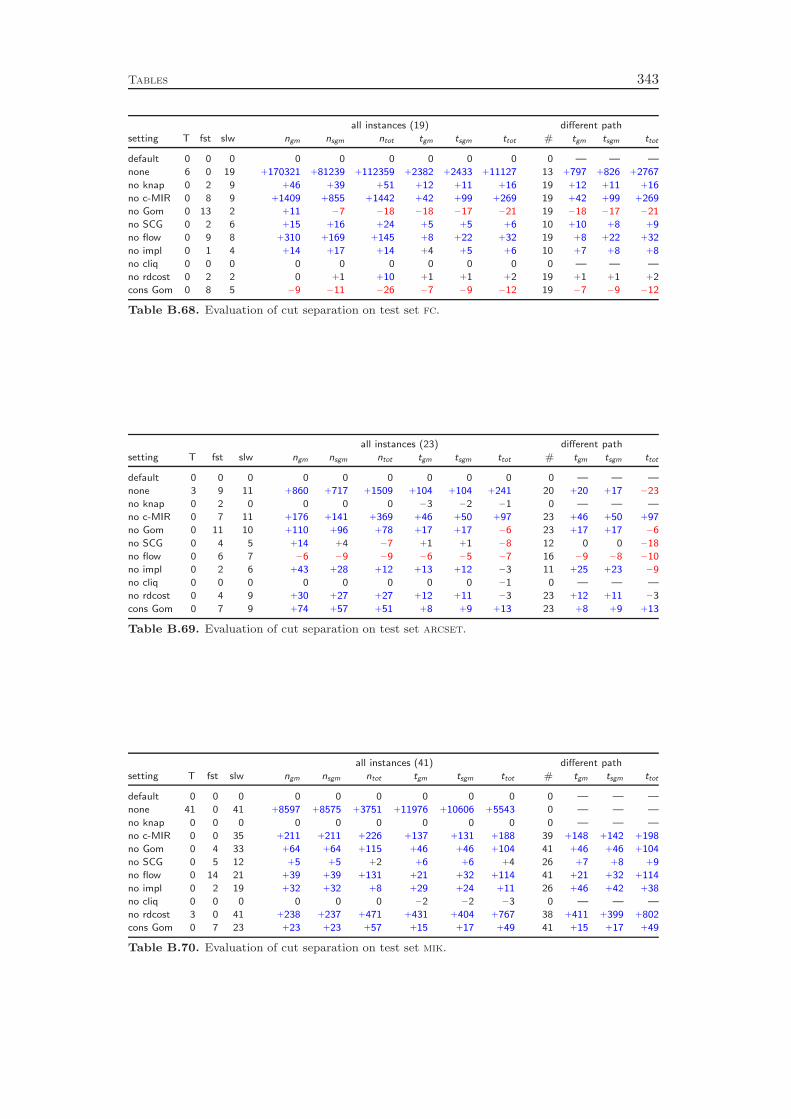
Tables 343
all instances (19) different path
setting T fst slw ngm nsgm ntot tgm tsgm ttot # tgm tsgm ttot
default 0 0 0 0 0 0 0 0 0 0 — — —
none 6 0 19 +170321 +81239 +112359 +2382 +2433 +11127 13 +797 +826 +2767
no knap 0 2 9 +46 +39 +51 +12 +11 +16 19 +12 +11 +16
no c-MIR 0 8 9 +1409 +855 +1442 +42 +99 +269 19 +42 +99 +269
no Gom 0 13 2 +11 −7 −18 −18 −17 −21 19 −18 −17 −21
no SCG 0 2 6 +15 +16 +24 +5 +5 +6 10 +10 +8 +9
no flow 0 9 8 +310 +169 +145 +8 +22 +32 19 +8 +22 +32
no impl 0 1 4 +14 +17 +14 +4 +5 +6 10 +7 +8 +8
no cliq 0 0 0 0 0 0 0 0 0 0 — — —
no rdcost 0 2 2 0 +1 +10 +1 +1 +2 19 +1 +1 +2
cons Gom 0 8 5 −9 −11 −26 −7 −9 −12 19 −7 −9 −12
Table B.68. Evaluation of cut separation on test set fc.
all instances (23) different path
setting T fst slw ngm nsgm ntot tgm tsgm ttot # tgm tsgm ttot
default 0 0 0 0 0 0 0 0 0 0 — — —
none 3 9 11 +860 +717 +1509 +104 +104 +241 20 +20 +17 −23
no knap 0 2 0 0 0 0 −3 −2 −1 0 — — —
no c-MIR 0 7 11 +176 +141 +369 +46 +50 +97 23 +46 +50 +97
no Gom 0 11 10 +110 +96 +78 +17 +17 −6 23 +17 +17 −6
no SCG 0 4 5 +14 +4 −7 +1 +1 −8 12 0 0 −18
no flow 0 6 7 −6 −9 −9 −6 −5 −7 16 −9 −8 −10
no impl 0 2 6 +43 +28 +12 +13 +12 −3 11 +25 +23 −9
no cliq 0 0 0 0 0 0 0 0 −1 0 — — —
no rdcost 0 4 9 +30 +27 +27 +12 +11 −3 23 +12 +11 −3
cons Gom 0 7 9 +74 +57 +51 +8 +9 +13 23 +8 +9 +13
Table B.69. Evaluation of cut separation on test set arcset.
all instances (41) different path
setting T fst slw ngm nsgm ntot tgm tsgm ttot # tgm tsgm ttot
default 0 0 0 0 0 0 0 0 0 0 — — —
none 41 0 41 +8597 +8575 +3751 +11976 +10606 +5543 0 — — —
no knap 0 0 0 0 0 0 0 0 0 0 — — —
no c-MIR 0 0 35 +211 +211 +226 +137 +131 +188 39 +148 +142 +198
no Gom 0 4 33 +64 +64 +115 +46 +46 +104 41 +46 +46 +104
no SCG 0 5 12 +5 +5 +2 +6 +6 +4 26 +7 +8 +9
no flow 0 14 21 +39 +39 +131 +21 +32 +114 41 +21 +32 +114
no impl 0 2 19 +32 +32 +8 +29 +24 +11 26 +46 +42 +38
no cliq 0 0 0 0 0 0 −2 −2 −3 0 — — —
no rdcost 3 0 41 +238 +237 +471 +431 +404 +767 38 +411 +399 +802
cons Gom 0 7 23 +23 +23 +57 +15 +17 +49 41 +15 +17 +49
Table B.70. Evaluation of cut separation on test set mik.
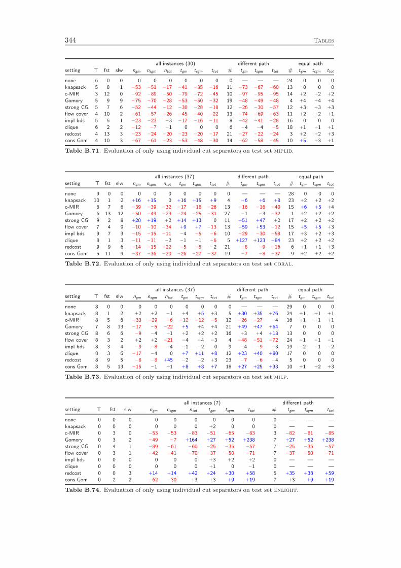
344 Tables
all instances (30) different path equal path
setting T fst slw ngm nsgm ntot tgm tsgm ttot # tgm tsgm ttot # tgm tsgm ttot
none 6 0 0 0 0 0 0 0 0 0 — — — 24 0 0 0
knapsack 5 8 1 −53 −51 −17 −41 −35 −16 11 −73 −67 −60 13 0 0 0
c-MIR 3 12 0 −92 −89 −50 −79 −72 −45 10 −97 −95 −95 14 +2 +2 +2
Gomory 5 9 9 −75 −70 −28 −53 −50 −32 19 −48 −49 −48 4 +4 +4 +4
strong CG 5 7 6 −52 −44 −12 −30 −28 −18 12 −26 −30 −57 12 +3 +3 +3
flow cover 4 10 2 −61 −57 −26 −45 −40 −22 13 −74 −69 −63 11 +2 +2 +1
impl bds 5 5 1 −23 −23 −3 −17 −16 −11 8 −42 −41 −28 16 0 0 0
clique 6 2 2 −12 −7 −1 0 0 0 6 −4 −4 −5 18 +1 +1 +1
redcost 4 13 3 −23 −24 −20 −23 −20 −17 21 −27 −22 −24 3 +2 +2 +3
cons Gom 4 10 3 −67 −61 −23 −53 −48 −30 14 −62 −58 −45 10 +5 +3 +1
Table B.71. Evaluation of only using individual cut separators on test set miplib.
all instances (37) different path equal path
setting T fst slw ngm nsgm ntot tgm tsgm ttot # tgm tsgm ttot # tgm tsgm ttot
none 9 0 0 0 0 0 0 0 0 0 — — — 28 0 0 0
knapsack 10 1 2 +16 +15 0 +16 +15 +9 4 +6 +6 +8 23 +2 +2 +2
c-MIR 6 7 6 −39 −39 −32 −17 −18 −26 13 −16 −16 −40 15 +6 +5 +4
Gomory 6 13 12 −50 −49 −29 −24 −25 −31 27 −1 −3 −32 1 +2 +2 +2
strong CG 9 2 8 +20 +19 +2 +14 +13 0 11 +51 +47 +2 17 +2 +2 +2
flow cover 7 4 9 −10 −10 −34 +9 +7 −13 13 +59 +53 −12 15 +5 +5 +3
impl bds 9 7 3 −15 −15 −11 −4 −5 −6 10 −29 −30 −58 17 +3 +2 +3
clique 8 1 3 −11 −11 −2 −1 −1 −6 5 +127 +123 +84 23 +2 +2 +2
redcost 9 9 6 −14 −15 −22 −5 −5 −2 21 −8 −9 −16 6 +1 +1 +3
cons Gom 5 11 9 −37 −36 −20 −26 −27 −37 19 −7 −8 −37 9 +2 +2 +2
Table B.72. Evaluation of only using individual cut separators on test set coral.
all instances (37) different path equal path
setting T fst slw ngm nsgm ntot tgm tsgm ttot # tgm tsgm ttot # tgm tsgm ttot
none 8 0 0 0 0 0 0 0 0 0 — — — 29 0 0 0
knapsack 8 1 2 +2 +2 −1 +4 +5 +3 5 +30 +35 +76 24 +1 +1 +1
c-MIR 8 5 6 −33 −29 −6 −12 −12 −5 12 −26 −27 −4 16 +1 +1 +1
Gomory 7 8 13 −17 −5 −22 +5 +4 +4 21 +49 +47 +64 7 0 0 0
strong CG 8 6 6 −9 −4 +1 +2 +2 +2 16 +3 +4 +13 13 0 0 0
flow cover 8 3 2 +2 +2 −21 −4 −4 −3 4 −48 −51 −72 24 −1 −1 −1
impl bds 8 3 4 −9 −8 +4 −1 −2 0 9 −4 −9 −3 19 −2 −1 −2
clique 8 3 6 −17 −4 0 +7 +11 +8 12 +23 +40 +80 17 0 0 0
redcost 8 9 5 −8 −8 +45 −2 −2 +3 23 −7 −6 −4 5 0 0 0
cons Gom 8 5 13 −15 −1 +1 +8 +8 +7 18 +27 +25 +33 10 +1 +2 +3
Table B.73. Evaluation of only using individual cut separators on test set milp.
all instances (7) different path
setting T fst slw ngm nsgm ntot tgm tsgm ttot # tgm tsgm ttot
none 0 0 0 0 0 0 0 0 0 0 — — —
knapsack 0 0 0 0 0 0 +2 0 0 0 — — —
c-MIR 0 3 0 −53 −53 −83 −51 −65 −83 3 −82 −81 −85
Gomory 0 3 2 −49 −7 +164 +27 +52 +238 7 +27 +52 +238
strong CG 0 4 1 −89 −61 −60 −25 −35 −57 7 −25 −35 −57
flow cover 0 3 1 −42 −41 −70 −37 −50 −71 7 −37 −50 −71
impl bds 0 0 0 0 0 0 +3 +2 +2 0 — — —
clique 0 0 0 0 0 0 +1 0 −1 0 — — —
redcost 0 0 3 +14 +14 +42 +24 +30 +58 5 +35 +38 +59
cons Gom 0 2 2 −62 −30 +3 +3 +9 +19 7 +3 +9 +19
Table B.74. Evaluation of only using individual cut separators on test set enlight.
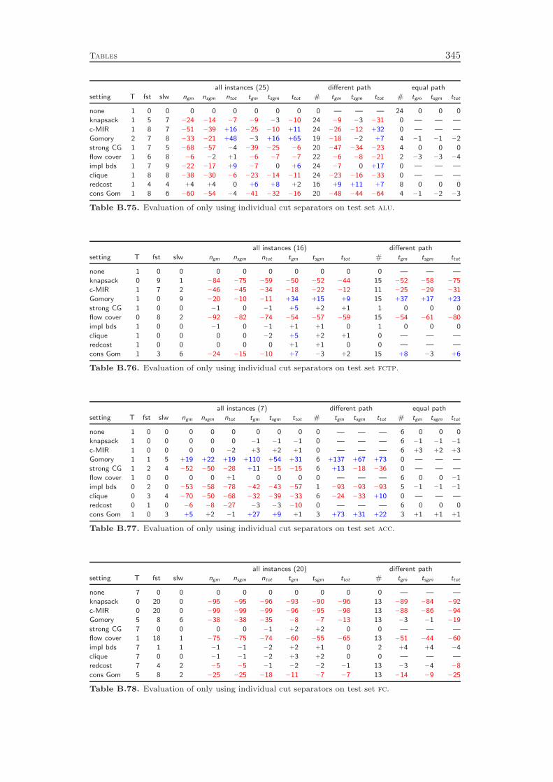
Tables 345
all instances (25) different path equal path
setting T fst slw ngm nsgm ntot tgm tsgm ttot # tgm tsgm ttot # tgm tsgm ttot
none 1 0 0 0 0 0 0 0 0 0 — — — 24 0 0 0
knapsack 1 5 7 −24 −14 −7 −9 −3 −10 24 −9 −3 −31 0 — — —
c-MIR 1 8 7 −51 −39 +16 −25 −10 +11 24 −26 −12 +32 0 — — —
Gomory 2 7 8 −33 −21 +48 −3 +16 +65 19 −18 −2 +7 4 −1 −1 −2
strong CG 1 7 5 −68 −57 −4 −39 −25 −6 20 −47 −34 −23 4 0 0 0
flow cover 1 6 8 −6 −2 +1 −6 −7 −7 22 −6 −8 −21 2 −3 −3 −4
impl bds 1 7 9 −22 −17 +9 −7 0 +6 24 −7 0 +17 0 — — —
clique 1 8 8 −38 −30 −6 −23 −14 −11 24 −23 −16 −33 0 — — —
redcost 1 4 4 +4 +4 0 +6 +8 +2 16 +9 +11 +7 8 0 0 0
cons Gom 1 8 6 −60 −54 −4 −41 −32 −16 20 −48 −44 −64 4 −1 −2 −3
Table B.75. Evaluation of only using individual cut separators on test set alu.
all instances (16) different path
setting T fst slw ngm nsgm ntot tgm tsgm ttot # tgm tsgm ttot
none 1 0 0 0 0 0 0 0 0 0 — — —
knapsack 0 9 1 −84 −75 −59 −50 −52 −44 15 −52 −58 −75
c-MIR 1 7 2 −46 −45 −34 −18 −22 −12 11 −25 −29 −31
Gomory 1 0 9 −20 −10 −11 +34 +15 +9 15 +37 +17 +23
strong CG 1 0 0 −1 0 −1 +5 +2 +1 1 0 0 0
flow cover 0 8 2 −92 −82 −74 −54 −57 −59 15 −54 −61 −80
impl bds 1 0 0 −1 0 −1 +1 +1 0 1 0 0 0
clique 1 0 0 0 0 −2 +5 +2 +1 0 — — —
redcost 1 0 0 0 0 0 +1 +1 0 0 — — —
cons Gom 1 3 6 −24 −15 −10 +7 −3 +2 15 +8 −3 +6
Table B.76. Evaluation of only using individual cut separators on test set fctp.
all instances (7) different path equal path
setting T fst slw ngm nsgm ntot tgm tsgm ttot # tgm tsgm ttot # tgm tsgm ttot
none 1 0 0 0 0 0 0 0 0 0 — — — 6 0 0 0
knapsack 1 0 0 0 0 0 −1 −1 −1 0 — — — 6 −1 −1 −1
c-MIR 1 0 0 0 0 −2 +3 +2 +1 0 — — — 6 +3 +2 +3
Gomory 1 1 5 +19 +22 +19 +110 +54 +31 6 +137 +67 +73 0 — — —
strong CG 1 2 4 −52 −50 −28 +11 −15 −15 6 +13 −18 −36 0 — — —
flow cover 1 0 0 0 0 +1 0 0 0 0 — — — 6 0 0 −1
impl bds 0 2 0 −53 −58 −78 −42 −43 −57 1 −93 −93 −93 5 −1 −1 −1
clique 0 3 4 −70 −50 −68 −32 −39 −33 6 −24 −33 +10 0 — — —
redcost 0 1 0 −6 −8 −27 −3 −3 −10 0 — — — 6 0 0 0
cons Gom 1 0 3 +5 +2 −1 +27 +9 +1 3 +73 +31 +22 3 +1 +1 +1
Table B.77. Evaluation of only using individual cut separators on test set acc.
all instances (20) different path
setting T fst slw ngm nsgm ntot tgm tsgm ttot # tgm tsgm ttot
none 7 0 0 0 0 0 0 0 0 0 — — —
knapsack 0 20 0 −95 −95 −96 −93 −90 −96 13 −89 −84 −92
c-MIR 0 20 0 −99 −99 −99 −96 −95 −98 13 −88 −86 −94
Gomory 5 8 6 −38 −38 −35 −8 −7 −13 13 −3 −1 −19
strong CG 7 0 0 0 0 −1 +2 +2 0 0 — — —
flow cover 1 18 1 −75 −75 −74 −60 −55 −65 13 −51 −44 −60
impl bds 7 1 1 −1 −1 −2 +2 +1 0 2 +4 +4 −4
clique 7 0 0 −1 −1 −2 +3 +2 0 0 — — —
redcost 7 4 2 −5 −5 −1 −2 −2 −1 13 −3 −4 −8
cons Gom 5 8 2 −25 −25 −18 −11 −7 −7 13 −14 −9 −25
Table B.78. Evaluation of only using individual cut separators on test set fc.
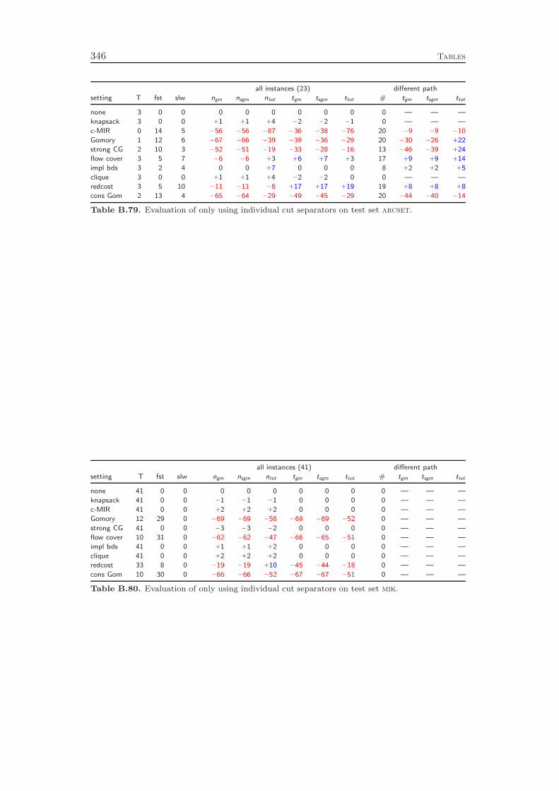
346 Tables
all instances (23) different path
setting T fst slw ngm nsgm ntot tgm tsgm ttot # tgm tsgm ttot
none 3 0 0 0 0 0 0 0 0 0 — — —
knapsack 3 0 0 +1 +1 +4 −2 −2 −1 0 — — —
c-MIR 0 14 5 −56 −56 −87 −36 −38 −76 20 −9 −9 −10
Gomory 1 12 6 −67 −66 −39 −39 −36 −29 20 −30 −26 +22
strong CG 2 10 3 −52 −51 −19 −33 −28 −16 13 −46 −39 +24
flow cover 3 5 7 −6 −6 +3 +6 +7 +3 17 +9 +9 +14
impl bds 3 2 4 0 0 +7 0 0 0 8 +2 +2 +5
clique 3 0 0 +1 +1 +4 −2 −2 0 0 — — —
redcost 3 5 10 −11 −11 −6 +17 +17 +19 19 +8 +8 +8
cons Gom 2 13 4 −65 −64 −29 −49 −45 −29 20 −44 −40 −14
Table B.79. Evaluation of only using individual cut separators on test set arcset.
all instances (41) different path
setting T fst slw ngm nsgm ntot tgm tsgm ttot # tgm tsgm ttot
none 41 0 0 0 0 0 0 0 0 0 — — —
knapsack 41 0 0 −1 −1 −1 0 0 0 0 — — —
c-MIR 41 0 0 +2 +2 +2 0 0 0 0 — — —
Gomory 12 29 0 −69 −69 −56 −69 −69 −52 0 — — —
strong CG 41 0 0 −3 −3 −2 0 0 0 0 — — —
flow cover 10 31 0 −62 −62 −47 −66 −65 −51 0 — — —
impl bds 41 0 0 +1 +1 +2 0 0 0 0 — — —
clique 41 0 0 +2 +2 +2 0 0 0 0 — — —
redcost 33 8 0 −19 −19 +10 −45 −44 −18 0 — — —
cons Gom 10 30 0 −66 −66 −52 −67 −67 −51 0 — — —
Table B.80. Evaluation of only using individual cut separators on test set mik.
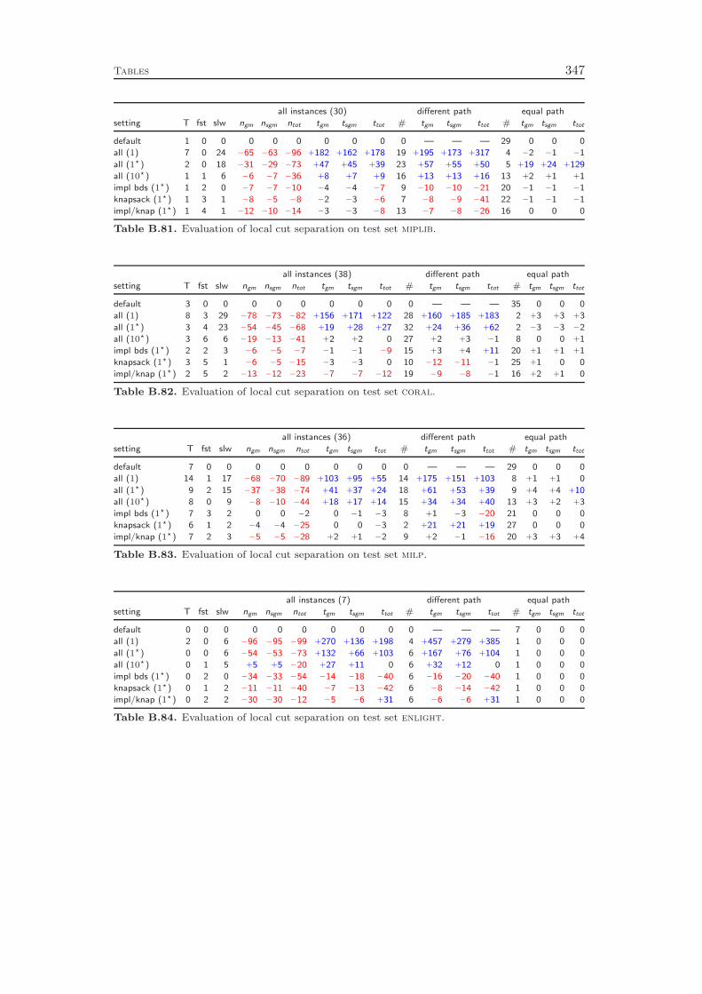
Tables 347
all instances (30) different path equal path
setting T fst slw ngm nsgm ntot tgm tsgm ttot # tgm tsgm ttot # tgm tsgm ttot
default 1 0 0 0 0 0 0 0 0 0 — — — 29 0 0 0
all (1) 7 0 24 −65 −63 −96 +182 +162 +178 19 +195 +173 +317 4 −2 −1 −1
all (1⋆) 2 0 18 −31 −29 −73 +47 +45 +39 23 +57 +55 +50 5 +19 +24 +129
all (10⋆) 1 1 6 −6 −7 −36 +8 +7 +9 16 +13 +13 +16 13 +2 +1 +1
impl bds (1⋆) 1 2 0 −7 −7 −10 −4 −4 −7 9 −10 −10 −21 20 −1 −1 −1
knapsack (1⋆) 1 3 1 −8 −5 −8 −2 −3 −6 7 −8 −9 −41 22 −1 −1 −1
impl/knap (1⋆) 1 4 1 −12 −10 −14 −3 −3 −8 13 −7 −8 −26 16 0 0 0
Table B.81. Evaluation of local cut separation on test set miplib.
all instances (38) different path equal path
setting T fst slw ngm nsgm ntot tgm tsgm ttot # tgm tsgm ttot # tgm tsgm ttot
default 3 0 0 0 0 0 0 0 0 0 — — — 35 0 0 0
all (1) 8 3 29 −78 −73 −82 +156 +171 +122 28 +160 +185 +183 2 +3 +3 +3
all (1⋆) 3 4 23 −54 −45 −68 +19 +28 +27 32 +24 +36 +62 2 −3 −3 −2
all (10⋆) 3 6 6 −19 −13 −41 +2 +2 0 27 +2 +3 −1 8 0 0 +1
impl bds (1⋆) 2 2 3 −6 −5 −7 −1 −1 −9 15 +3 +4 +11 20 +1 +1 +1
knapsack (1⋆) 3 5 1 −6 −5 −15 −3 −3 0 10 −12 −11 −1 25 +1 0 0
impl/knap (1⋆) 2 5 2 −13 −12 −23 −7 −7 −12 19 −9 −8 −1 16 +2 +1 0
Table B.82. Evaluation of local cut separation on test set coral.
all instances (36) different path equal path
setting T fst slw ngm nsgm ntot tgm tsgm ttot # tgm tsgm ttot # tgm tsgm ttot
default 7 0 0 0 0 0 0 0 0 0 — — — 29 0 0 0
all (1) 14 1 17 −68 −70 −89 +103 +95 +55 14 +175 +151 +103 8 +1 +1 0
all (1⋆) 9 2 15 −37 −38 −74 +41 +37 +24 18 +61 +53 +39 9 +4 +4 +10
all (10⋆) 8 0 9 −8 −10 −44 +18 +17 +14 15 +34 +34 +40 13 +3 +2 +3
impl bds (1⋆) 7 3 2 0 0 −2 0 −1 −3 8 +1 −3 −20 21 0 0 0
knapsack (1⋆) 6 1 2 −4 −4 −25 0 0 −3 2 +21 +21 +19 27 0 0 0
impl/knap (1⋆) 7 2 3 −5 −5 −28 +2 +1 −2 9 +2 −1 −16 20 +3 +3 +4
Table B.83. Evaluation of local cut separation on test set milp.
all instances (7) different path equal path
setting T fst slw ngm nsgm ntot tgm tsgm ttot # tgm tsgm ttot # tgm tsgm ttot
default 0 0 0 0 0 0 0 0 0 0 — — — 7 0 0 0
all (1) 2 0 6 −96 −95 −99 +270 +136 +198 4 +457 +279 +385 1 0 0 0
all (1⋆) 0 0 6 −54 −53 −73 +132 +66 +103 6 +167 +76 +104 1 0 0 0
all (10⋆) 0 1 5 +5 +5 −20 +27 +11 0 6 +32 +12 0 1 0 0 0
impl bds (1⋆) 0 2 0 −34 −33 −54 −14 −18 −40 6 −16 −20 −40 1 0 0 0
knapsack (1⋆) 0 1 2 −11 −11 −40 −7 −13 −42 6 −8 −14 −42 1 0 0 0
impl/knap (1⋆) 0 2 2 −30 −30 −12 −5 −6 +31 6 −6 −6 +31 1 0 0 0
Table B.84. Evaluation of local cut separation on test set enlight.
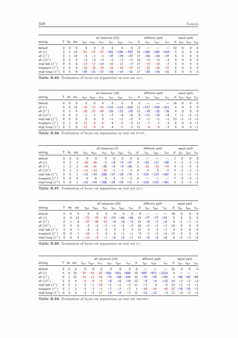
348 Tables
all instances (22) different path equal path
setting T fst slw ngm nsgm ntot tgm tsgm ttot # tgm tsgm ttot # tgm tsgm ttot
default 0 0 0 0 0 0 0 0 0 0 — — — 22 0 0 0
all (1) 2 2 13 −51 −47 −47 +201 +196 +537 15 +290 +249 +510 5 0 0 0
all (1⋆) 0 1 14 −4 +1 −3 +37 +29 +37 17 +50 +34 +37 5 0 0 0
all (10⋆) 0 2 3 +3 +3 +3 +2 +2 +3 13 +4 +3 +3 9 0 0 0
impl bds (1⋆) 0 4 8 −15 −17 +13 −10 −13 +7 17 −13 −14 +7 5 0 0 0
knapsack (1⋆) 0 6 4 −10 −16 −18 −16 −25 −27 17 −20 −28 −27 5 0 0 0
impl/knap (1⋆) 0 6 8 +26 +21 +17 +26 +14 +31 17 +35 +16 +31 5 0 0 0
Table B.85. Evaluation of local cut separation on test set alu.
all instances (16) different path equal path
setting T fst slw ngm nsgm ntot tgm tsgm ttot # tgm tsgm ttot # tgm tsgm ttot
default 0 0 0 0 0 0 0 0 0 0 — — — 16 0 0 0
all (1) 0 0 12 −76 −72 −92 +115 +123 +310 12 +177 +158 +311 4 0 0 0
all (1⋆) 0 2 9 −26 −22 −40 +25 +21 +35 12 +35 +25 +35 4 0 0 0
all (10⋆) 0 0 3 −1 −1 −5 +7 +8 +8 9 +11 +10 +8 7 +1 +2 +2
impl bds (1⋆) 0 0 0 0 0 0 +1 +1 +2 3 +1 +1 +1 13 +1 +1 +2
knapsack (1⋆) 0 2 0 −12 −9 −5 −4 −5 −3 11 −7 −7 −3 5 0 0 +1
impl/knap (1⋆) 0 2 0 −12 −8 −5 −4 −5 −2 11 −6 −6 −2 5 0 0 +1
Table B.86. Evaluation of local cut separation on test set fctp.
all instances (7) different path equal path
setting T fst slw ngm nsgm ntot tgm tsgm ttot # tgm tsgm ttot # tgm tsgm ttot
default 0 0 0 0 0 0 0 0 0 0 — — — 7 0 0 0
all (1) 0 2 2 −46 −45 −2 +8 +9 +57 4 +16 +17 +58 3 −2 −2 −2
all (1⋆) 1 2 2 −44 −41 +25 +8 +9 +66 3 −34 −34 −43 3 −3 −3 −3
all (10⋆) 0 2 1 −21 −23 −20 −1 −1 −3 4 0 0 −3 3 −2 −2 −2
impl bds (1⋆) 0 0 1 +21 +43 +288 +27 +28 +75 2 +124 +127 +307 5 +1 +1 +1
knapsack (1⋆) 0 0 0 0 0 0 −3 −2 −2 0 — — — 7 −3 −2 −2
impl/knap (1⋆) 0 0 1 +21 +43 +288 +24 +25 +71 2 +120 +122 +301 5 −2 −2 −2
Table B.87. Evaluation of local cut separation on test set acc.
all instances (20) different path equal path
setting T fst slw ngm nsgm ntot tgm tsgm ttot # tgm tsgm ttot # tgm tsgm ttot
default 0 0 0 0 0 0 0 0 0 0 — — — 20 0 0 0
all (1) 0 0 13 −72 −78 −91 +53 +62 +86 15 +77 +77 +93 5 0 0 0
all (1⋆) 0 1 6 −37 −36 −51 +6 +6 +5 15 +8 +7 +6 5 −1 −1 −1
all (10⋆) 0 0 0 −2 −2 −1 +1 +1 +2 10 +2 +2 +3 10 0 0 0
impl bds (1⋆) 0 0 1 −4 −4 0 0 0 0 11 0 0 +1 9 0 0 0
knapsack (1⋆) 0 0 1 −10 −7 0 0 +1 +1 8 +1 +2 +4 12 0 0 0
impl/knap (1⋆) 0 0 4 −13 −9 −1 +6 +6 +7 14 +6 +6 +8 6 +3 +3 +4
Table B.88. Evaluation of local cut separation on test set fc.
all instances (23) different path equal path
setting T fst slw ngm nsgm ntot tgm tsgm ttot # tgm tsgm ttot # tgm tsgm ttot
default 0 0 0 0 0 0 0 0 0 0 — — — 23 0 0 0
all (1) 4 0 23 −47 −45 −47 +681 +631 +600 19 +697 +671 +1223 0 — — —
all (1⋆) 0 1 22 −10 −11 −16 +75 +69 +106 22 +75 +70 +106 1 +65 +65 +65
all (10⋆) 0 0 4 −6 −6 −6 +6 +6 +14 13 +8 +8 +15 10 +2 +2 +3
impl bds (1⋆) 0 2 1 0 −1 −10 +1 +1 −3 11 +1 0 −8 12 +1 +1 +1
knapsack (1⋆) 0 1 2 −3 −3 −1 +7 +7 +7 1 −40 −40 −40 22 +10 +10 +7
impl/knap (1⋆) 0 3 6 −3 −4 −11 +8 +8 +2 11 +13 +13 +3 12 +4 +3 +2
Table B.89. Evaluation of local cut separation on test set arcset.

Tables 349
all instances (41) different path
setting T fst slw ngm nsgm ntot tgm tsgm ttot # tgm tsgm ttot
default 0 0 0 0 0 0 0 0 0 0 — — —
all (1) 0 6 29 −91 −91 −93 +63 +56 +30 41 +63 +56 +30
all (1⋆) 0 26 5 −69 −69 −74 −28 −29 −42 41 −28 −29 −42
all (10⋆) 0 21 3 −30 −30 −25 −12 −12 −13 41 −12 −12 −13
impl bds (1⋆) 0 0 0 0 0 0 +2 +2 +2 12 +2 +2 +2
knapsack (1⋆) 0 24 4 −43 −42 −38 −25 −23 −29 41 −25 −23 −29
impl/knap (1⋆) 0 22 11 −43 −43 −38 −20 −18 −24 41 −20 −18 −24
Table B.90. Evaluation of local cut separation on test set mik.
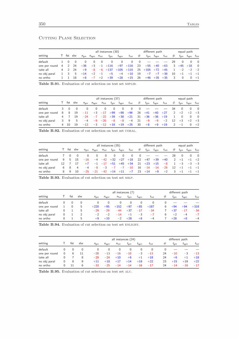
350 Tables
Cutting Plane Selection
all instances (30) different path equal path
setting T fst slw ngm nsgm ntot tgm tsgm ttot # tgm tsgm ttot # tgm tsgm ttot
default 1 0 0 0 0 0 0 0 0 0 — — — 29 0 0 0
one per round 4 2 24 +36 +3 −1 +116 +97 +116 23 +55 +40 +63 3 +45 +18 0
take all 4 2 24 +9 −8 −6 +137 +105 +110 25 +105 +72 +45 1 −2 −2 −2
no obj paral 1 3 5 +14 +2 −1 +5 +4 +10 19 +7 +7 +38 10 +1 +1 +1
no ortho 1 1 18 +8 −7 +2 +39 +28 +15 26 +46 +35 +35 3 0 0 +1
Table B.91. Evaluation of cut selection on test set miplib.
all instances (37) different path equal path
setting T fst slw ngm nsgm ntot tgm tsgm ttot # tgm tsgm ttot # tgm tsgm ttot
default 3 0 0 0 0 0 0 0 0 0 — — — 34 0 0 0
one per round 8 8 19 −11 +3 −17 +99 +98 +96 26 +41 +40 +27 2 +2 +2 +3
take all 4 7 19 −24 −7 −22 +39 +38 +21 31 +36 +36 +19 1 0 0 0
no obj paral 3 9 5 −4 −9 −20 −8 −8 −4 21 −9 −9 −2 12 +3 +2 +3
no ortho 4 10 19 −12 −3 −12 +18 +19 +25 30 +8 +9 +19 2 −1 0 +2
Table B.92. Evaluation of cut selection on test set coral.
all instances (35) different path equal path
setting T fst slw ngm nsgm ntot tgm tsgm ttot # tgm tsgm ttot # tgm tsgm ttot
default 7 0 0 0 0 0 0 0 0 0 — — — 28 0 0 0
one per round 9 5 15 −16 −4 −42 +32 +27 +18 22 +47 +39 +40 2 +1 +1 +2
take all 12 7 17 +7 −1 −17 +51 +45 +34 21 +23 +15 −8 1 −3 −3 −3
no obj paral 6 8 4 −4 −8 −3 −7 −7 −10 16 −14 −14 −25 12 +1 +1 +1
no ortho 8 9 10 −25 −21 −42 +14 +11 +7 23 +14 +9 +2 3 +1 +1 +1
Table B.93. Evaluation of cut selection on test set milp.
all instances (7) different path
setting T fst slw ngm nsgm ntot tgm tsgm ttot # tgm tsgm ttot
default 0 0 0 0 0 0 0 0 0 0 — — —
one per round 1 0 5 +220 +95 +152 +97 +85 +187 6 +94 +94 +318
take all 0 1 5 −29 −29 −44 +37 −17 −34 7 +37 −17 −34
no obj paral 0 1 2 −2 −2 −14 +1 −3 −7 6 +2 −4 −7
no ortho 0 1 5 +9 +10 −2 +28 +8 −4 7 +28 +8 −4
Table B.94. Evaluation of cut selection on test set enlight.
all instances (24) different path
setting T fst slw ngm nsgm ntot tgm tsgm ttot # tgm tsgm ttot
default 0 0 0 0 0 0 0 0 0 0 — — —
one per round 0 6 11 −20 −13 −16 −10 −3 −13 24 −10 −3 −13
take all 0 7 8 −29 −24 +10 +6 +1 +18 24 +6 +1 +18
no obj paral 0 8 9 +11 +18 +17 +14 +18 +22 23 +15 +19 +22
no ortho 0 11 6 −33 −25 −14 −14 −16 −17 24 −14 −16 −17
Table B.95. Evaluation of cut selection on test set alu.
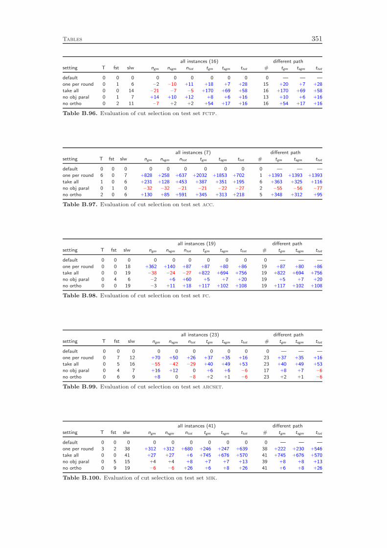
Tables 351
all instances (16) different path
setting T fst slw ngm nsgm ntot tgm tsgm ttot # tgm tsgm ttot
default 0 0 0 0 0 0 0 0 0 0 — — —
one per round 0 1 6 −2 −10 +11 +18 +7 +28 15 +20 +7 +28
take all 0 0 14 −21 −7 −5 +170 +69 +58 16 +170 +69 +58
no obj paral 0 1 7 +14 +10 +12 +8 +6 +16 13 +10 +6 +16
no ortho 0 2 11 −7 +2 +2 +54 +17 +16 16 +54 +17 +16
Table B.96. Evaluation of cut selection on test set fctp.
all instances (7) different path
setting T fst slw ngm nsgm ntot tgm tsgm ttot # tgm tsgm ttot
default 0 0 0 0 0 0 0 0 0 0 — — —
one per round 6 0 7 +828 +258 +637 +2032 +1853 +702 1 +1393 +1393 +1393
take all 1 0 6 +231 +128 +453 +387 +351 +195 6 +363 +325 +116
no obj paral 0 1 0 −32 −32 −21 −21 −22 −27 2 −55 −56 −77
no ortho 2 0 6 +130 +85 +591 +345 +313 +218 5 +348 +312 +95
Table B.97. Evaluation of cut selection on test set acc.
all instances (19) different path
setting T fst slw ngm nsgm ntot tgm tsgm ttot # tgm tsgm ttot
default 0 0 0 0 0 0 0 0 0 0 — — —
one per round 0 0 18 +362 +140 +87 +87 +80 +86 19 +87 +80 +86
take all 0 0 19 −38 −24 −27 +822 +694 +756 19 +822 +694 +756
no obj paral 0 4 6 −2 +6 +60 +5 +7 +20 19 +5 +7 +20
no ortho 0 0 19 −3 +11 +18 +117 +102 +108 19 +117 +102 +108
Table B.98. Evaluation of cut selection on test set fc.
all instances (23) different path
setting T fst slw ngm nsgm ntot tgm tsgm ttot # tgm tsgm ttot
default 0 0 0 0 0 0 0 0 0 0 — — —
one per round 0 7 12 +70 +50 +26 +37 +35 +16 23 +37 +35 +16
take all 0 5 16 −55 −42 −29 +40 +49 +53 23 +40 +49 +53
no obj paral 0 4 7 +16 +12 0 +6 +6 −6 17 +8 +7 −6
no ortho 0 6 9 +8 0 −8 +2 +1 −6 23 +2 +1 −6
Table B.99. Evaluation of cut selection on test set arcset.
all instances (41) different path
setting T fst slw ngm nsgm ntot tgm tsgm ttot # tgm tsgm ttot
default 0 0 0 0 0 0 0 0 0 0 — — —
one per round 3 2 38 +312 +312 +680 +246 +247 +639 38 +222 +230 +546
take all 0 0 41 +27 +27 +6 +745 +676 +570 41 +745 +676 +570
no obj paral 0 5 15 +4 +4 +8 +7 +7 +13 39 +8 +8 +13
no ortho 0 9 19 −6 −6 +26 +6 +8 +26 41 +6 +8 +26
Table B.100. Evaluation of cut selection on test set mik.
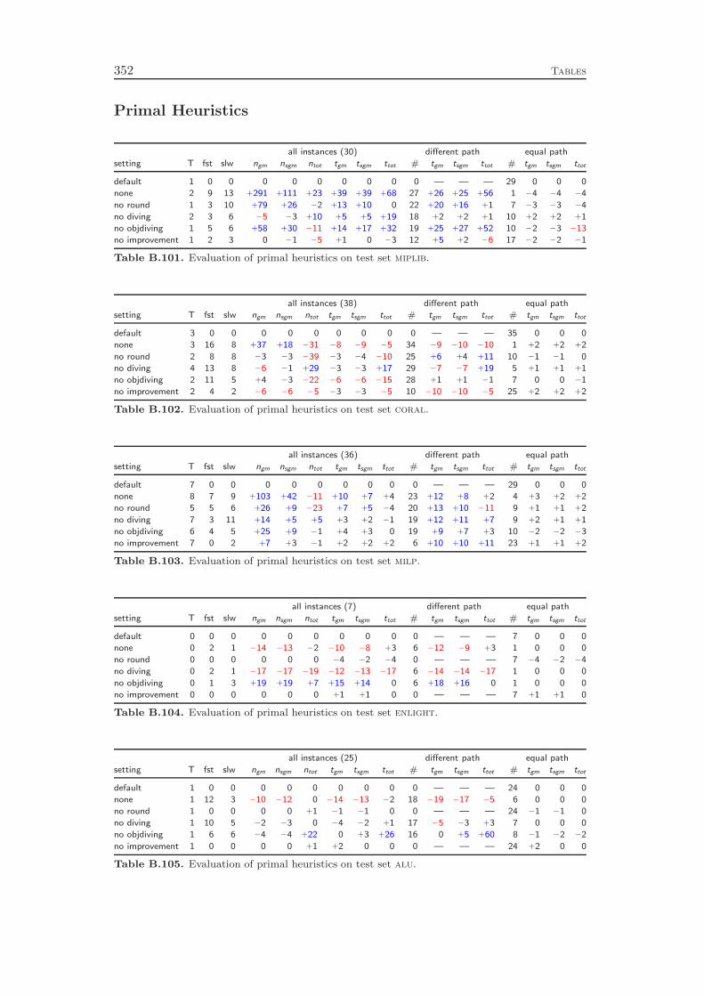
352 Tables
Primal Heuristics
all instances (30) different path equal path
setting T fst slw ngm nsgm ntot tgm tsgm ttot # tgm tsgm ttot # tgm tsgm ttot
default 1 0 0 0 0 0 0 0 0 0 — — — 29 0 0 0
none 2 9 13 +291 +111 +23 +39 +39 +68 27 +26 +25 +56 1 −4 −4 −4
no round 1 3 10 +79 +26 −2 +13 +10 0 22 +20 +16 +1 7 −3 −3 −4
no diving 2 3 6 −5 −3 +10 +5 +5 +19 18 +2 +2 +1 10 +2 +2 +1
no objdiving 1 5 6 +58 +30 −11 +14 +17 +32 19 +25 +27 +52 10 −2 −3 −13
no improvement 1 2 3 0 −1 −5 +1 0 −3 12 +5 +2 −6 17 −2 −2 −1
Table B.101. Evaluation of primal heuristics on test set miplib.
all instances (38) different path equal path
setting T fst slw ngm nsgm ntot tgm tsgm ttot # tgm tsgm ttot # tgm tsgm ttot
default 3 0 0 0 0 0 0 0 0 0 — — — 35 0 0 0
none 3 16 8 +37 +18 −31 −8 −9 −5 34 −9 −10 −10 1 +2 +2 +2
no round 2 8 8 −3 −3 −39 −3 −4 −10 25 +6 +4 +11 10 −1 −1 0
no diving 4 13 8 −6 −1 +29 −3 −3 +17 29 −7 −7 +19 5 +1 +1 +1
no objdiving 2 11 5 +4 −3 −22 −6 −6 −15 28 +1 +1 −1 7 0 0 −1
no improvement 2 4 2 −6 −6 −5 −3 −3 −5 10 −10 −10 −5 25 +2 +2 +2
Table B.102. Evaluation of primal heuristics on test set coral.
all instances (36) different path equal path
setting T fst slw ngm nsgm ntot tgm tsgm ttot # tgm tsgm ttot # tgm tsgm ttot
default 7 0 0 0 0 0 0 0 0 0 — — — 29 0 0 0
none 8 7 9 +103 +42 −11 +10 +7 +4 23 +12 +8 +2 4 +3 +2 +2
no round 5 5 6 +26 +9 −23 +7 +5 −4 20 +13 +10 −11 9 +1 +1 +2
no diving 7 3 11 +14 +5 +5 +3 +2 −1 19 +12 +11 +7 9 +2 +1 +1
no objdiving 6 4 5 +25 +9 −1 +4 +3 0 19 +9 +7 +3 10 −2 −2 −3
no improvement 7 0 2 +7 +3 −1 +2 +2 +2 6 +10 +10 +11 23 +1 +1 +2
Table B.103. Evaluation of primal heuristics on test set milp.
all instances (7) different path equal path
setting T fst slw ngm nsgm ntot tgm tsgm ttot # tgm tsgm ttot # tgm tsgm ttot
default 0 0 0 0 0 0 0 0 0 0 — — — 7 0 0 0
none 0 2 1 −14 −13 −2 −10 −8 +3 6 −12 −9 +3 1 0 0 0
no round 0 0 0 0 0 0 −4 −2 −4 0 — — — 7 −4 −2 −4
no diving 0 2 1 −17 −17 −19 −12 −13 −17 6 −14 −14 −17 1 0 0 0
no objdiving 0 1 3 +19 +19 +7 +15 +14 0 6 +18 +16 0 1 0 0 0
no improvement 0 0 0 0 0 0 +1 +1 0 0 — — — 7 +1 +1 0
Table B.104. Evaluation of primal heuristics on test set enlight.
all instances (25) different path equal path
setting T fst slw ngm nsgm ntot tgm tsgm ttot # tgm tsgm ttot # tgm tsgm ttot
default 1 0 0 0 0 0 0 0 0 0 — — — 24 0 0 0
none 1 12 3 −10 −12 0 −14 −13 −2 18 −19 −17 −5 6 0 0 0
no round 1 0 0 0 0 +1 −1 −1 0 0 — — — 24 −1 −1 0
no diving 1 10 5 −2 −3 0 −4 −2 +1 17 −5 −3 +3 7 0 0 0
no objdiving 1 6 6 −4 −4 +22 0 +3 +26 16 0 +5 +60 8 −1 −2 −2
no improvement 1 0 0 0 0 +1 +2 0 0 0 — — — 24 +2 0 0
Table B.105. Evaluation of primal heuristics on test set alu.

Tables 353
all instances (16) different path equal path
setting T fst slw ngm nsgm ntot tgm tsgm ttot # tgm tsgm ttot # tgm tsgm ttot
default 0 0 0 0 0 0 0 0 0 0 — — — 16 0 0 0
none 0 2 6 +208 +84 +19 +13 +3 −2 13 +16 +3 −2 3 0 0 0
no round 0 4 4 +71 +35 −1 +9 +1 −2 12 +12 +1 −2 4 0 0 0
no diving 0 1 6 0 0 +5 +6 +4 +3 9 +8 +6 +3 7 +3 +5 +5
no objdiving 0 3 0 −2 −2 −2 0 −2 0 8 −3 −3 0 8 +3 +4 +4
no improvement 0 1 3 +4 +4 0 +5 +4 +5 6 +8 +6 +5 10 +4 +3 +5
Table B.106. Evaluation of primal heuristics on test set fctp.
all instances (7) different path equal path
setting T fst slw ngm nsgm ntot tgm tsgm ttot # tgm tsgm ttot # tgm tsgm ttot
default 0 0 0 0 0 0 0 0 0 0 — — — 7 0 0 0
none 0 2 5 +957 +151 +427 +42 +35 +48 7 +42 +35 +48 0 — — —
no round 0 0 0 0 0 0 −3 −3 −4 0 — — — 7 −3 −3 −4
no diving 0 2 1 −15 −5 +330 −9 −9 +35 3 −18 −17 +38 4 −1 −1 −1
no objdiving 0 2 5 +1094 +158 +262 +70 +62 +33 7 +70 +62 +33 0 — — —
no improvement 0 0 0 0 0 0 −2 −2 −2 0 — — — 7 −2 −2 −2
Table B.107. Evaluation of primal heuristics on test set acc.
all instances (20) different path equal path
setting T fst slw ngm nsgm ntot tgm tsgm ttot # tgm tsgm ttot # tgm tsgm ttot
default 0 0 0 0 0 0 0 0 0 0 — — — 20 0 0 0
none 0 0 20 +1761 +774 +536 +83 +82 +107 20 +83 +82 +107 0 — — —
no round 0 1 13 +274 +139 +60 +19 +21 +24 18 +22 +23 +26 2 −6 −6 −6
no diving 0 0 0 −2 −2 −1 +3 +3 +3 10 +3 +3 +3 10 +3 +3 +3
no objdiving 0 1 0 −2 −2 −6 0 −1 −3 8 −3 −3 −4 12 +2 +2 +2
no improvement 0 2 1 −10 −10 −7 0 0 0 12 −1 −1 0 8 +2 +2 +2
Table B.108. Evaluation of primal heuristics on test set fc.
all instances (23) different path equal path
setting T fst slw ngm nsgm ntot tgm tsgm ttot # tgm tsgm ttot # tgm tsgm ttot
default 0 0 0 0 0 0 0 0 0 0 — — — 23 0 0 0
none 0 10 6 +72 +53 +42 +2 +2 −14 23 +2 +2 −14 0 — — —
no round 0 5 5 +18 +10 −9 +1 +1 −9 23 +1 +1 −9 0 — — —
no diving 0 4 7 +6 +5 −5 0 −1 −18 23 0 −1 −18 0 — — —
no objdiving 0 6 5 +5 +4 +12 +1 +1 +6 19 +1 +1 +6 4 −1 −1 0
no improvement 0 5 5 0 +1 +5 +1 +1 −1 13 +3 +3 −2 10 −1 −1 +1
Table B.109. Evaluation of primal heuristics on test set arcset.
all instances (41) different path equal path
setting T fst slw ngm nsgm ntot tgm tsgm ttot # tgm tsgm ttot # tgm tsgm ttot
default 0 0 0 0 0 0 0 0 0 0 — — — 41 0 0 0
none 2 0 41 +380 +379 +551 +524 +481 +832 39 +519 +487 +950 0 — — —
no round 0 16 21 +24 +24 −8 +29 +23 −1 41 +29 +23 −1 0 — — —
no diving 0 11 6 +10 +10 +22 0 +2 +16 41 0 +2 +16 0 — — —
no objdiving 0 6 10 0 0 +7 +4 +4 +11 41 +4 +4 +11 0 — — —
no improvement 0 1 3 +1 +1 +8 +1 +2 +10 23 +1 +2 +11 18 +1 +1 +1
Table B.110. Evaluation of primal heuristics on test set mik.
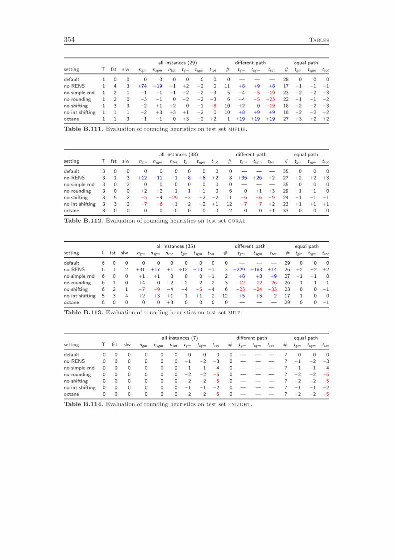
354 Tables
all instances (29) different path equal path
setting T fst slw ngm nsgm ntot tgm tsgm ttot # tgm tsgm ttot # tgm tsgm ttot
default 1 0 0 0 0 0 0 0 0 0 — — — 28 0 0 0
no RENS 1 4 3 +74 +19 −1 +2 +2 0 11 +8 +9 +8 17 −1 −1 −1
no simple rnd 1 2 1 −1 −1 +1 −2 −2 −3 5 −4 −5 −19 23 −2 −2 −3
no rounding 1 2 0 +3 −1 0 −2 −2 −3 6 −4 −5 −23 22 −1 −1 −2
no shifting 1 3 3 −2 +1 +2 0 −1 −8 10 +2 0 −19 18 −2 −2 −3
no int shifting 1 1 1 +2 +3 +3 +1 +2 0 10 +8 +9 +9 18 −2 −2 −2
octane 1 1 3 −1 −1 0 +3 +2 +2 1 +19 +19 +19 27 +3 +2 +2
Table B.111. Evaluation of rounding heuristics on test set miplib.
all instances (38) different path equal path
setting T fst slw ngm nsgm ntot tgm tsgm ttot # tgm tsgm ttot # tgm tsgm ttot
default 3 0 0 0 0 0 0 0 0 0 — — — 35 0 0 0
no RENS 3 1 3 +12 +11 −1 +8 +6 +2 8 +36 +26 +2 27 +2 +2 +3
no simple rnd 3 0 2 0 0 0 0 0 0 0 — — — 35 0 0 0
no rounding 3 0 0 +2 +2 −1 −1 −1 0 6 0 +1 +3 29 −1 −1 0
no shifting 3 5 2 −5 −4 −29 −3 −2 −2 11 −6 −6 −9 24 −1 −1 −1
no int shifting 3 3 2 −7 −6 +1 −2 −2 +1 12 −7 −7 +2 23 +1 +1 +1
octane 3 0 0 0 0 0 0 0 0 2 0 0 +1 33 0 0 0
Table B.112. Evaluation of rounding heuristics on test set coral.
all instances (35) different path equal path
setting T fst slw ngm nsgm ntot tgm tsgm ttot # tgm tsgm ttot # tgm tsgm ttot
default 6 0 0 0 0 0 0 0 0 0 — — — 29 0 0 0
no RENS 6 1 2 +31 +17 +1 +12 +10 +1 3 +229 +183 +14 26 +2 +2 +2
no simple rnd 6 0 0 +1 +1 0 0 0 +1 2 +8 +8 +9 27 −1 −1 0
no rounding 6 1 0 +4 0 −2 −2 −2 −2 3 −12 −12 −26 26 −1 −1 −1
no shifting 6 2 1 −7 −9 −4 −4 −5 −4 6 −23 −24 −33 23 0 0 −1
no int shifting 5 3 4 +2 +3 +1 +1 +1 −2 12 +5 +5 −2 17 −1 0 0
octane 6 0 0 0 0 +3 0 0 0 0 — — — 29 0 0 −1
Table B.113. Evaluation of rounding heuristics on test set milp.
all instances (7) different path equal path
setting T fst slw ngm nsgm ntot tgm tsgm ttot # tgm tsgm ttot # tgm tsgm ttot
default 0 0 0 0 0 0 0 0 0 0 — — — 7 0 0 0
no RENS 0 0 0 0 0 0 −1 −2 −3 0 — — — 7 −1 −2 −3
no simple rnd 0 0 0 0 0 0 −1 −1 −4 0 — — — 7 −1 −1 −4
no rounding 0 0 0 0 0 0 −2 −2 −5 0 — — — 7 −2 −2 −5
no shifting 0 0 0 0 0 0 −2 −2 −5 0 — — — 7 −2 −2 −5
no int shifting 0 0 0 0 0 0 −1 −1 −2 0 — — — 7 −1 −1 −2
octane 0 0 0 0 0 0 −2 −2 −5 0 — — — 7 −2 −2 −5
Table B.114. Evaluation of rounding heuristics on test set enlight.
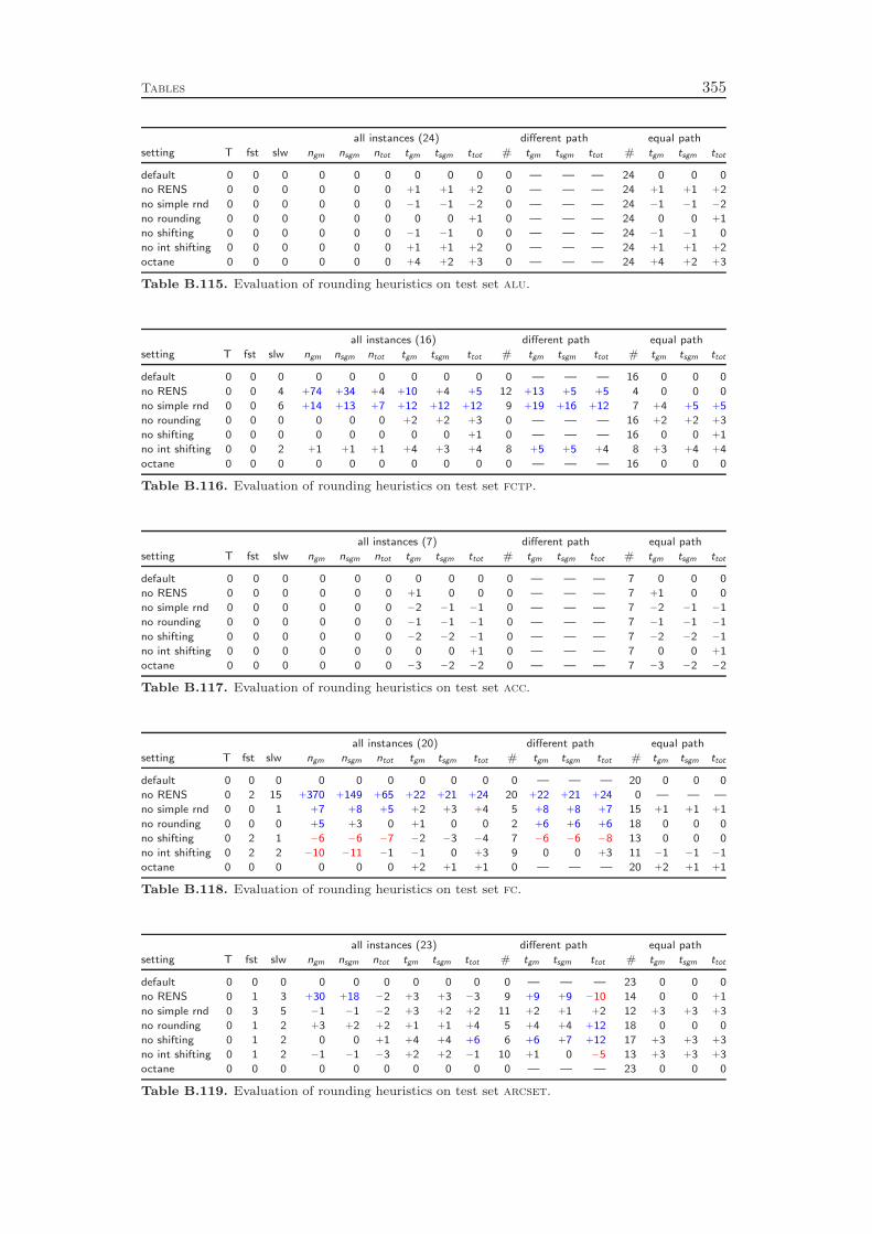
Tables 355
all instances (24) different path equal path
setting T fst slw ngm nsgm ntot tgm tsgm ttot # tgm tsgm ttot # tgm tsgm ttot
default 0 0 0 0 0 0 0 0 0 0 — — — 24 0 0 0
no RENS 0 0 0 0 0 0 +1 +1 +2 0 — — — 24 +1 +1 +2
no simple rnd 0 0 0 0 0 0 −1 −1 −2 0 — — — 24 −1 −1 −2
no rounding 0 0 0 0 0 0 0 0 +1 0 — — — 24 0 0 +1
no shifting 0 0 0 0 0 0 −1 −1 0 0 — — — 24 −1 −1 0
no int shifting 0 0 0 0 0 0 +1 +1 +2 0 — — — 24 +1 +1 +2
octane 0 0 0 0 0 0 +4 +2 +3 0 — — — 24 +4 +2 +3
Table B.115. Evaluation of rounding heuristics on test set alu.
all instances (16) different path equal path
setting T fst slw ngm nsgm ntot tgm tsgm ttot # tgm tsgm ttot # tgm tsgm ttot
default 0 0 0 0 0 0 0 0 0 0 — — — 16 0 0 0
no RENS 0 0 4 +74 +34 +4 +10 +4 +5 12 +13 +5 +5 4 0 0 0
no simple rnd 0 0 6 +14 +13 +7 +12 +12 +12 9 +19 +16 +12 7 +4 +5 +5
no rounding 0 0 0 0 0 0 +2 +2 +3 0 — — — 16 +2 +2 +3
no shifting 0 0 0 0 0 0 0 0 +1 0 — — — 16 0 0 +1
no int shifting 0 0 2 +1 +1 +1 +4 +3 +4 8 +5 +5 +4 8 +3 +4 +4
octane 0 0 0 0 0 0 0 0 0 0 — — — 16 0 0 0
Table B.116. Evaluation of rounding heuristics on test set fctp.
all instances (7) different path equal path
setting T fst slw ngm nsgm ntot tgm tsgm ttot # tgm tsgm ttot # tgm tsgm ttot
default 0 0 0 0 0 0 0 0 0 0 — — — 7 0 0 0
no RENS 0 0 0 0 0 0 +1 0 0 0 — — — 7 +1 0 0
no simple rnd 0 0 0 0 0 0 −2 −1 −1 0 — — — 7 −2 −1 −1
no rounding 0 0 0 0 0 0 −1 −1 −1 0 — — — 7 −1 −1 −1
no shifting 0 0 0 0 0 0 −2 −2 −1 0 — — — 7 −2 −2 −1
no int shifting 0 0 0 0 0 0 0 0 +1 0 — — — 7 0 0 +1
octane 0 0 0 0 0 0 −3 −2 −2 0 — — — 7 −3 −2 −2
Table B.117. Evaluation of rounding heuristics on test set acc.
all instances (20) different path equal path
setting T fst slw ngm nsgm ntot tgm tsgm ttot # tgm tsgm ttot # tgm tsgm ttot
default 0 0 0 0 0 0 0 0 0 0 — — — 20 0 0 0
no RENS 0 2 15 +370 +149 +65 +22 +21 +24 20 +22 +21 +24 0 — — —
no simple rnd 0 0 1 +7 +8 +5 +2 +3 +4 5 +8 +8 +7 15 +1 +1 +1
no rounding 0 0 0 +5 +3 0 +1 0 0 2 +6 +6 +6 18 0 0 0
no shifting 0 2 1 −6 −6 −7 −2 −3 −4 7 −6 −6 −8 13 0 0 0
no int shifting 0 2 2 −10 −11 −1 −1 0 +3 9 0 0 +3 11 −1 −1 −1
octane 0 0 0 0 0 0 +2 +1 +1 0 — — — 20 +2 +1 +1
Table B.118. Evaluation of rounding heuristics on test set fc.
all instances (23) different path equal path
setting T fst slw ngm nsgm ntot tgm tsgm ttot # tgm tsgm ttot # tgm tsgm ttot
default 0 0 0 0 0 0 0 0 0 0 — — — 23 0 0 0
no RENS 0 1 3 +30 +18 −2 +3 +3 −3 9 +9 +9 −10 14 0 0 +1
no simple rnd 0 3 5 −1 −1 −2 +3 +2 +2 11 +2 +1 +2 12 +3 +3 +3
no rounding 0 1 2 +3 +2 +2 +1 +1 +4 5 +4 +4 +12 18 0 0 0
no shifting 0 1 2 0 0 +1 +4 +4 +6 6 +6 +7 +12 17 +3 +3 +3
no int shifting 0 1 2 −1 −1 −3 +2 +2 −1 10 +1 0 −5 13 +3 +3 +3
octane 0 0 0 0 0 0 0 0 0 0 — — — 23 0 0 0
Table B.119. Evaluation of rounding heuristics on test set arcset.
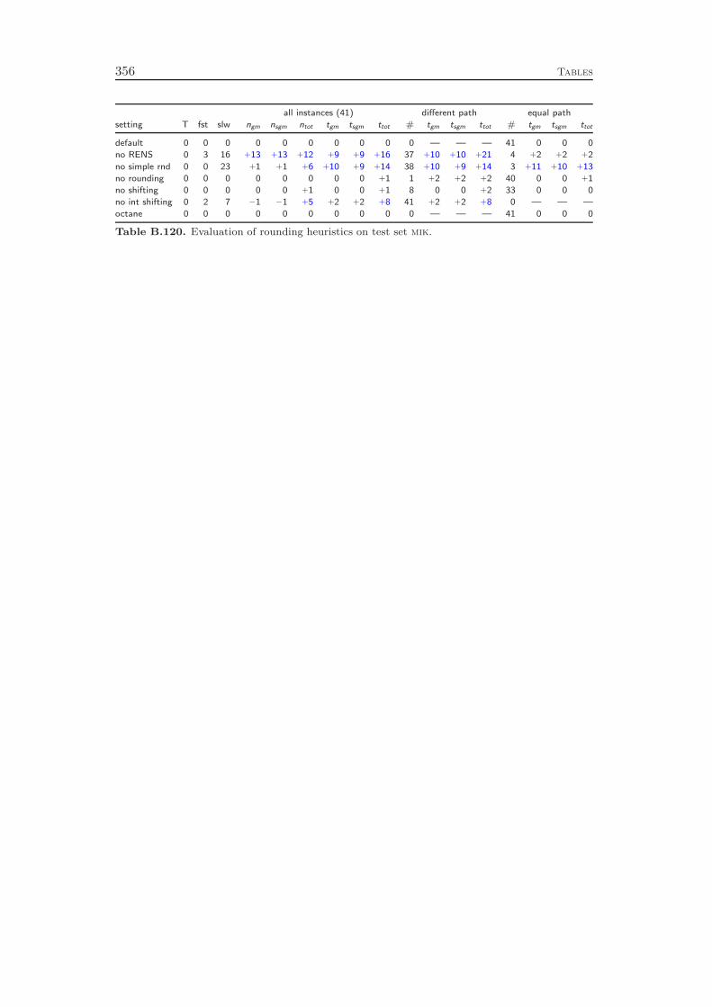
356 Tables
all instances (41) different path equal path
setting T fst slw ngm nsgm ntot tgm tsgm ttot # tgm tsgm ttot # tgm tsgm ttot
default 0 0 0 0 0 0 0 0 0 0 — — — 41 0 0 0
no RENS 0 3 16 +13 +13 +12 +9 +9 +16 37 +10 +10 +21 4 +2 +2 +2
no simple rnd 0 0 23 +1 +1 +6 +10 +9 +14 38 +10 +9 +14 3 +11 +10 +13
no rounding 0 0 0 0 0 0 0 0 +1 1 +2 +2 +2 40 0 0 +1
no shifting 0 0 0 0 0 +1 0 0 +1 8 0 0 +2 33 0 0 0
no int shifting 0 2 7 −1 −1 +5 +2 +2 +8 41 +2 +2 +8 0 — — —
octane 0 0 0 0 0 0 0 0 0 0 — — — 41 0 0 0
Table B.120. Evaluation of rounding heuristics on test set mik.

Tables 357
all instances (30) different path equal path
setting T fst slw ngm nsgm ntot tgm tsgm ttot # tgm tsgm ttot # tgm tsgm ttot
default 1 0 0 0 0 0 0 0 0 0 — — — 29 0 0 0
no coef 1 3 6 +1 +1 +3 +1 0 +3 19 +2 +1 +4 10 −1 −1 −2
no frac 1 5 2 −3 −3 −14 −6 −6 −13 18 −9 −9 −20 11 −1 −1 −1
no guided 1 3 1 0 0 −7 −2 −2 −9 14 −3 −3 −13 15 −2 −2 −7
no linesearch 1 1 1 0 0 +1 −1 −1 +1 14 0 0 +3 15 −2 −2 −8
no pscost 1 5 2 −3 −3 −7 −4 −4 −9 19 −6 −6 −13 10 −2 −1 −1
no veclen 1 5 1 −3 −3 −3 −3 −3 −3 16 −5 −4 −4 13 −2 −2 −8
no backtrack 1 6 3 −6 −6 −6 −4 −4 −6 18 −5 −6 −9 11 −2 −1 −1
Table B.121. Evaluation of diving heuristics on test set miplib.
all instances (38) different path equal path
setting T fst slw ngm nsgm ntot tgm tsgm ttot # tgm tsgm ttot # tgm tsgm ttot
default 3 0 0 0 0 0 0 0 0 0 — — — 35 0 0 0
no coef 3 15 4 −18 −13 −10 −8 −8 −1 30 −10 −10 −2 5 0 0 0
no frac 3 7 4 −1 0 −12 0 0 0 28 −1 −1 −1 7 +3 +3 +3
no guided 2 9 2 −4 −4 −14 −6 −6 −5 24 −9 −9 −9 11 −1 −1 −1
no linesearch 2 5 6 +4 +4 −4 +4 +4 −1 26 +7 +6 +5 9 +3 +3 +3
no pscost 3 10 3 −9 −5 −12 −3 −3 −3 29 −4 −4 −7 6 −1 −1 −1
no veclen 2 10 4 −8 −7 −22 −7 −7 −15 27 +1 +2 +1 8 0 0 0
no backtrack 3 11 4 +3 +2 −16 −1 −3 −4 29 −2 −3 −7 6 −1 −1 −1
Table B.122. Evaluation of diving heuristics on test set coral.
all instances (35) different path equal path
setting T fst slw ngm nsgm ntot tgm tsgm ttot # tgm tsgm ttot # tgm tsgm ttot
default 6 0 0 0 0 0 0 0 0 0 — — — 29 0 0 0
no coef 6 5 4 −7 −7 +2 −2 −2 +1 18 −8 −8 −10 10 0 0 0
no frac 5 4 4 +4 +4 +2 +1 +1 −1 16 +4 +4 +3 13 −1 0 0
no guided 5 1 8 +16 +16 +2 +11 +10 +9 15 +25 +25 +33 14 +2 +2 +2
no linesearch 6 0 8 +9 +10 0 +6 +6 +5 15 +15 +14 +17 14 0 0 0
no pscost 6 2 4 0 0 −1 +1 0 −1 16 +2 +1 −2 13 −1 −1 −1
no veclen 6 2 2 +2 +2 +6 +1 +2 +2 15 +3 +3 +7 14 0 0 0
no backtrack 5 2 5 +5 +5 +4 +3 +3 0 17 +7 +6 +1 12 +1 +1 +2
Table B.123. Evaluation of diving heuristics on test set milp.
all instances (7) different path equal path
setting T fst slw ngm nsgm ntot tgm tsgm ttot # tgm tsgm ttot # tgm tsgm ttot
default 0 0 0 0 0 0 0 0 0 0 — — — 7 0 0 0
no coef 0 2 3 +3 +3 +6 +4 +4 +1 6 +5 +4 +1 1 0 0 0
no frac 0 1 2 +6 +6 −12 +3 −4 −17 6 +4 −5 −17 1 0 0 0
no guided 0 0 0 +2 +2 +2 +2 +2 +2 4 +4 +4 +8 3 0 −1 −1
no linesearch 0 1 2 +12 +13 +30 +10 +13 +28 6 +11 +14 +28 1 0 0 0
no pscost 0 0 3 +19 +19 +11 +19 +18 +11 6 +22 +20 +11 1 0 0 0
no veclen 0 0 3 +12 +12 +17 +10 +9 +14 6 +12 +10 +14 1 0 0 0
no backtrack 0 2 3 +10 +11 +29 +16 +19 +30 6 +19 +21 +30 1 0 0 0
Table B.124. Evaluation of diving heuristics on test set enlight.

358 Tables
all instances (25) different path equal path
setting T fst slw ngm nsgm ntot tgm tsgm ttot # tgm tsgm ttot # tgm tsgm ttot
default 1 0 0 0 0 0 0 0 0 0 — — — 24 0 0 0
no coef 1 2 10 +54 +52 +24 +35 +36 +42 17 +56 +53 +97 7 0 0 0
no frac 1 2 8 +3 +3 +3 0 −1 +3 16 0 −2 +6 8 0 0 0
no guided 1 0 0 0 0 +1 0 0 0 0 — — — 24 0 0 +1
no linesearch 1 4 9 +25 +22 +3 +11 +8 +4 16 +17 +11 +9 8 0 0 0
no pscost 1 5 6 +8 +6 −1 0 −2 −6 16 +1 −3 −14 8 0 0 0
no veclen 1 4 7 +11 +11 +4 +6 +5 +8 16 +9 +7 +19 8 0 0 0
no backtrack 1 8 5 −1 −2 0 −4 −5 +2 16 −6 −7 +4 8 0 0 0
Table B.125. Evaluation of diving heuristics on test set alu.
all instances (16) different path equal path
setting T fst slw ngm nsgm ntot tgm tsgm ttot # tgm tsgm ttot # tgm tsgm ttot
default 0 0 0 0 0 0 0 0 0 0 — — — 16 0 0 0
no coef 0 2 1 −3 −3 −1 −2 −3 −3 9 −5 −5 −3 7 +1 +2 +2
no frac 0 0 3 +1 +1 +4 +5 +4 +8 8 +5 +5 +8 8 +4 +5 +6
no guided 0 2 0 −3 −4 −1 −2 −3 −1 8 −5 −5 −1 8 +1 +1 +1
no linesearch 0 0 1 0 0 0 +2 +2 +2 8 +2 +2 +2 8 +2 +3 +3
no pscost 0 0 1 +1 +1 +3 +1 +1 +2 8 +2 +2 +2 8 +1 +1 +1
no veclen 0 2 1 −2 −2 −3 +1 0 +1 8 0 −1 +1 8 +3 +4 +4
no backtrack 0 1 0 −3 −3 −7 0 −2 −4 8 −2 −3 −4 8 +3 +4 +4
Table B.126. Evaluation of diving heuristics on test set fctp.
all instances (7) different path equal path
setting T fst slw ngm nsgm ntot tgm tsgm ttot # tgm tsgm ttot # tgm tsgm ttot
default 0 0 0 0 0 0 0 0 0 0 — — — 7 0 0 0
no coef 0 1 2 +37 +72 +498 +18 +19 +95 3 +53 +54 +105 4 −3 −3 −3
no frac 1 1 2 +28 +48 +458 +12 +13 +77 2 −39 −39 −31 4 −2 −2 −2
no guided 0 0 0 0 0 0 −2 −2 −2 0 — — — 7 −2 −2 −2
no linesearch 1 2 1 +29 +48 +582 +14 +15 +78 2 −34 −34 −30 4 −3 −3 −3
no pscost 1 1 2 +49 +73 +441 +40 +42 +142 2 +30 +30 +57 4 −2 −2 −2
no veclen 0 0 2 +35 +50 +135 +16 +16 +30 3 +40 +40 +33 4 +1 +1 0
no backtrack 0 2 1 +14 +26 +314 +12 +12 +39 3 +27 +27 +43 4 +1 +1 +1
Table B.127. Evaluation of diving heuristics on test set acc.
all instances (20) different path equal path
setting T fst slw ngm nsgm ntot tgm tsgm ttot # tgm tsgm ttot # tgm tsgm ttot
default 0 0 0 0 0 0 0 0 0 0 — — — 20 0 0 0
no coef 0 1 0 −2 −2 −8 −1 −1 −2 10 −2 −2 −3 10 0 0 0
no frac 0 0 0 0 −1 0 0 0 0 10 0 0 0 10 0 0 0
no guided 0 0 0 0 0 −1 0 0 0 6 0 0 −1 14 0 0 0
no linesearch 0 0 0 0 0 −1 0 0 0 6 0 0 0 14 0 0 0
no pscost 0 0 0 +1 +1 +2 0 +1 +1 10 +1 +1 +2 10 0 0 0
no veclen 0 0 1 +1 +1 +8 +1 +1 +2 8 +1 +1 +2 12 +1 +1 0
no backtrack 0 1 0 −1 −1 −3 0 0 −1 8 0 −1 −1 12 +1 +1 +1
Table B.128. Evaluation of diving heuristics on test set fc.
all instances (23) different path equal path
setting T fst slw ngm nsgm ntot tgm tsgm ttot # tgm tsgm ttot # tgm tsgm ttot
default 0 0 0 0 0 0 0 0 0 0 — — — 23 0 0 0
no coef 0 6 6 +7 +6 +12 +6 +5 −7 23 +6 +5 −7 0 — — —
no frac 0 5 2 −6 −6 −9 −3 −3 −8 20 −3 −3 −8 3 +1 +1 +1
no guided 0 4 3 0 0 −4 +1 +1 −4 16 0 0 −4 7 +2 +2 +2
no linesearch 0 4 4 +2 +2 0 +1 +1 0 16 0 +1 0 7 +1 +1 +1
no pscost 0 3 5 +8 +8 +18 +9 +10 +5 20 +10 +11 +5 3 +3 +3 +3
no veclen 0 6 3 −7 −8 −3 −5 −5 +4 20 −6 −6 +4 3 0 0 0
no backtrack 0 5 6 +11 +11 +12 +6 +6 +4 22 +6 +6 +4 1 +2 +2 +2
Table B.129. Evaluation of diving heuristics on test set arcset.

Tables 359
all instances (41) different path
setting T fst slw ngm nsgm ntot tgm tsgm ttot # tgm tsgm ttot
default 0 0 0 0 0 0 0 0 0 0 — — —
no coef 0 5 9 0 0 +6 +2 +2 +7 41 +2 +2 +7
no frac 0 6 9 0 0 +3 +2 +1 +6 41 +2 +1 +6
no guided 0 2 1 0 0 +1 +1 0 +1 20 0 0 +2
no linesearch 0 5 6 0 0 +11 +3 +4 +15 41 +3 +4 +15
no pscost 0 4 7 −1 −1 +8 +2 +2 +11 41 +2 +2 +11
no veclen 0 7 6 −2 −2 +1 0 0 +3 41 0 0 +3
no backtrack 0 4 10 +4 +4 +7 +2 +2 +7 41 +2 +2 +7
Table B.130. Evaluation of diving heuristics on test set mik.
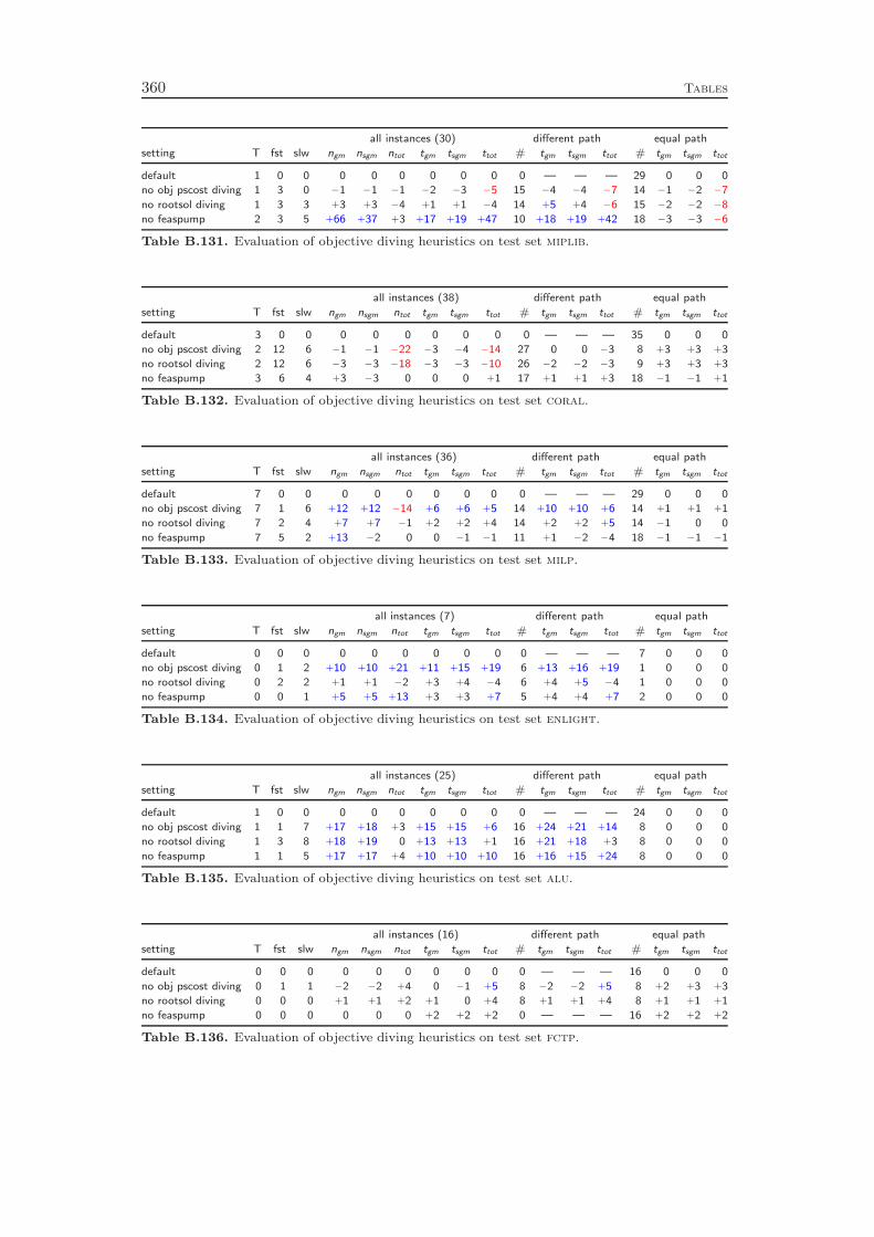
360 Tables
all instances (30) different path equal path
setting T fst slw ngm nsgm ntot tgm tsgm ttot # tgm tsgm ttot # tgm tsgm ttot
default 1 0 0 0 0 0 0 0 0 0 — — — 29 0 0 0
no obj pscost diving 1 3 0 −1 −1 −1 −2 −3 −5 15 −4 −4 −7 14 −1 −2 −7
no rootsol diving 1 3 3 +3 +3 −4 +1 +1 −4 14 +5 +4 −6 15 −2 −2 −8
no feaspump 2 3 5 +66 +37 +3 +17 +19 +47 10 +18 +19 +42 18 −3 −3 −6
Table B.131. Evaluation of objective diving heuristics on test set miplib.
all instances (38) different path equal path
setting T fst slw ngm nsgm ntot tgm tsgm ttot # tgm tsgm ttot # tgm tsgm ttot
default 3 0 0 0 0 0 0 0 0 0 — — — 35 0 0 0
no obj pscost diving 2 12 6 −1 −1 −22 −3 −4 −14 27 0 0 −3 8 +3 +3 +3
no rootsol diving 2 12 6 −3 −3 −18 −3 −3 −10 26 −2 −2 −3 9 +3 +3 +3
no feaspump 3 6 4 +3 −3 0 0 0 +1 17 +1 +1 +3 18 −1 −1 +1
Table B.132. Evaluation of objective diving heuristics on test set coral.
all instances (36) different path equal path
setting T fst slw ngm nsgm ntot tgm tsgm ttot # tgm tsgm ttot # tgm tsgm ttot
default 7 0 0 0 0 0 0 0 0 0 — — — 29 0 0 0
no obj pscost diving 7 1 6 +12 +12 −14 +6 +6 +5 14 +10 +10 +6 14 +1 +1 +1
no rootsol diving 7 2 4 +7 +7 −1 +2 +2 +4 14 +2 +2 +5 14 −1 0 0
no feaspump 7 5 2 +13 −2 0 0 −1 −1 11 +1 −2 −4 18 −1 −1 −1
Table B.133. Evaluation of objective diving heuristics on test set milp.
all instances (7) different path equal path
setting T fst slw ngm nsgm ntot tgm tsgm ttot # tgm tsgm ttot # tgm tsgm ttot
default 0 0 0 0 0 0 0 0 0 0 — — — 7 0 0 0
no obj pscost diving 0 1 2 +10 +10 +21 +11 +15 +19 6 +13 +16 +19 1 0 0 0
no rootsol diving 0 2 2 +1 +1 −2 +3 +4 −4 6 +4 +5 −4 1 0 0 0
no feaspump 0 0 1 +5 +5 +13 +3 +3 +7 5 +4 +4 +7 2 0 0 0
Table B.134. Evaluation of objective diving heuristics on test set enlight.
all instances (25) different path equal path
setting T fst slw ngm nsgm ntot tgm tsgm ttot # tgm tsgm ttot # tgm tsgm ttot
default 1 0 0 0 0 0 0 0 0 0 — — — 24 0 0 0
no obj pscost diving 1 1 7 +17 +18 +3 +15 +15 +6 16 +24 +21 +14 8 0 0 0
no rootsol diving 1 3 8 +18 +19 0 +13 +13 +1 16 +21 +18 +3 8 0 0 0
no feaspump 1 1 5 +17 +17 +4 +10 +10 +10 16 +16 +15 +24 8 0 0 0
Table B.135. Evaluation of objective diving heuristics on test set alu.
all instances (16) different path equal path
setting T fst slw ngm nsgm ntot tgm tsgm ttot # tgm tsgm ttot # tgm tsgm ttot
default 0 0 0 0 0 0 0 0 0 0 — — — 16 0 0 0
no obj pscost diving 0 1 1 −2 −2 +4 0 −1 +5 8 −2 −2 +5 8 +2 +3 +3
no rootsol diving 0 0 0 +1 +1 +2 +1 0 +4 8 +1 +1 +4 8 +1 +1 +1
no feaspump 0 0 0 0 0 0 +2 +2 +2 0 — — — 16 +2 +2 +2
Table B.136. Evaluation of objective diving heuristics on test set fctp.
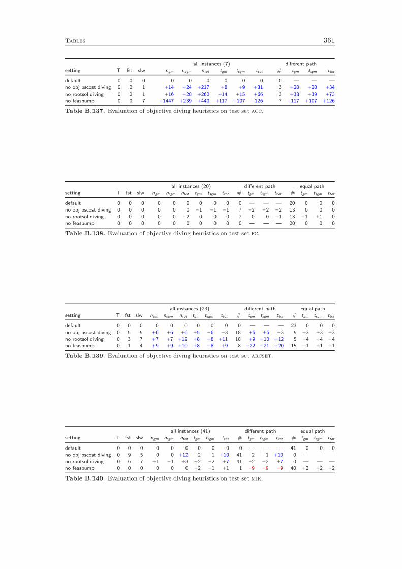
Tables 361
all instances (7) different path
setting T fst slw ngm nsgm ntot tgm tsgm ttot # tgm tsgm ttot
default 0 0 0 0 0 0 0 0 0 0 — — —
no obj pscost diving 0 2 1 +14 +24 +217 +8 +9 +31 3 +20 +20 +34
no rootsol diving 0 2 1 +16 +28 +262 +14 +15 +66 3 +38 +39 +73
no feaspump 0 0 7 +1447 +239 +440 +117 +107 +126 7 +117 +107 +126
Table B.137. Evaluation of objective diving heuristics on test set acc.
all instances (20) different path equal path
setting T fst slw ngm nsgm ntot tgm tsgm ttot # tgm tsgm ttot # tgm tsgm ttot
default 0 0 0 0 0 0 0 0 0 0 — — — 20 0 0 0
no obj pscost diving 0 0 0 0 0 0 −1 −1 −1 7 −2 −2 −2 13 0 0 0
no rootsol diving 0 0 0 0 0 −2 0 0 0 7 0 0 −1 13 +1 +1 0
no feaspump 0 0 0 0 0 0 0 0 0 0 — — — 20 0 0 0
Table B.138. Evaluation of objective diving heuristics on test set fc.
all instances (23) different path equal path
setting T fst slw ngm nsgm ntot tgm tsgm ttot # tgm tsgm ttot # tgm tsgm ttot
default 0 0 0 0 0 0 0 0 0 0 — — — 23 0 0 0
no obj pscost diving 0 5 5 +6 +6 +6 +5 +6 −3 18 +6 +6 −3 5 +3 +3 +3
no rootsol diving 0 3 7 +7 +7 +12 +8 +8 +11 18 +9 +10 +12 5 +4 +4 +4
no feaspump 0 1 4 +9 +9 +10 +8 +8 +9 8 +22 +21 +20 15 +1 +1 +1
Table B.139. Evaluation of objective diving heuristics on test set arcset.
all instances (41) different path equal path
setting T fst slw ngm nsgm ntot tgm tsgm ttot # tgm tsgm ttot # tgm tsgm ttot
default 0 0 0 0 0 0 0 0 0 0 — — — 41 0 0 0
no obj pscost diving 0 9 5 0 0 +12 −2 −1 +10 41 −2 −1 +10 0 — — —
no rootsol diving 0 6 7 −1 −1 +3 +2 +2 +7 41 +2 +2 +7 0 — — —
no feaspump 0 0 0 0 0 0 +2 +1 +1 1 −9 −9 −9 40 +2 +2 +2
Table B.140. Evaluation of objective diving heuristics on test set mik.

362 Tables
all instances (30) different path equal path
setting T fst slw ngm nsgm ntot tgm tsgm ttot # tgm tsgm ttot # tgm tsgm ttot
default 1 0 0 0 0 0 0 0 0 0 — — — 29 0 0 0
no oneopt 1 2 2 −3 −4 −11 0 −1 −6 8 +4 −1 −22 21 −2 −2 −3
no crossover 1 2 1 −2 −2 −6 −4 −4 −7 5 −15 −17 −18 24 −1 −1 −1
local branching 1 2 5 −4 −4 −7 +1 0 −4 7 −8 −10 −16 22 +4 +4 +7
RINS 1 1 2 −1 −1 −8 −1 −1 −7 8 −1 −3 −15 21 −1 −1 −2
mutation 1 3 1 −2 −2 −9 0 −1 −7 9 −5 −7 −16 20 +2 +1 +3
Table B.141. Evaluation of improvement heuristics on test set miplib.
all instances (37) different path equal path
setting T fst slw ngm nsgm ntot tgm tsgm ttot # tgm tsgm ttot # tgm tsgm ttot
default 3 0 0 0 0 0 0 0 0 0 — — — 34 0 0 0
no oneopt 3 1 1 −1 −1 −2 +1 +1 +1 4 −6 −7 −13 30 +2 +2 +2
no crossover 3 3 1 −4 −4 0 −2 −2 0 8 −12 −12 −3 26 +1 +1 +2
local branching 3 2 3 −4 −4 0 +1 +1 +1 8 −6 −6 +2 26 +3 +3 +2
RINS 2 4 0 −9 −9 −10 −5 −5 −13 10 −8 −7 −3 24 +2 +2 +3
mutation 3 3 0 −4 −4 −1 −3 −3 −1 10 −10 −9 −5 24 0 0 +1
Table B.142. Evaluation of improvement heuristics on test set coral.
all instances (35) different path equal path
setting T fst slw ngm nsgm ntot tgm tsgm ttot # tgm tsgm ttot # tgm tsgm ttot
default 6 0 0 0 0 0 0 0 0 0 — — — 29 0 0 0
no oneopt 6 0 0 +5 +2 +1 −1 0 0 2 +2 +2 +1 27 −1 −1 −1
no crossover 6 0 2 +2 +2 0 +1 +1 +2 5 +9 +9 +11 24 0 0 0
local branching 6 0 8 +1 +1 −2 +6 +5 +4 6 +14 +14 +16 23 +5 +5 +4
RINS 6 0 2 0 0 −2 +2 +2 +2 7 +5 +5 +9 22 +1 +1 +1
mutation 6 0 1 +1 +1 +7 +2 +1 +1 5 +4 +4 +3 24 +1 +1 +2
Table B.143. Evaluation of improvement heuristics on test set milp.
all instances (7) different path equal path
setting T fst slw ngm nsgm ntot tgm tsgm ttot # tgm tsgm ttot # tgm tsgm ttot
default 0 0 0 0 0 0 0 0 0 0 — — — 7 0 0 0
no oneopt 0 0 0 0 0 0 −3 −3 −6 0 — — — 7 −3 −3 −6
no crossover 0 0 0 0 0 0 +1 −1 −2 0 — — — 7 +1 −1 −2
local branching 0 0 1 0 0 0 +6 +1 −1 0 — — — 7 +6 +1 −1
RINS 0 0 0 0 0 0 +2 +1 +2 0 — — — 7 +2 +1 +2
mutation 0 0 0 0 0 0 −2 −2 −5 0 — — — 7 −2 −2 −5
Table B.144. Evaluation of improvement heuristics on test set enlight.
all instances (24) different path equal path
setting T fst slw ngm nsgm ntot tgm tsgm ttot # tgm tsgm ttot # tgm tsgm ttot
default 0 0 0 0 0 0 0 0 0 0 — — — 24 0 0 0
no oneopt 0 0 0 0 0 0 −1 −1 −1 0 — — — 24 −1 −1 −1
no crossover 0 0 0 0 0 0 +1 0 +1 0 — — — 24 +1 0 +1
local branching 0 0 0 0 0 0 −1 −1 −1 0 — — — 24 −1 −1 −1
RINS 0 0 0 0 0 0 0 0 0 0 — — — 24 0 0 0
mutation 0 0 0 0 0 0 +1 0 +1 0 — — — 24 +1 0 +1
Table B.145. Evaluation of improvement heuristics on test set alu.
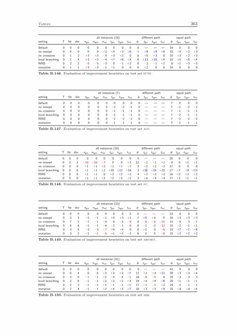
Tables 363
all instances (16) different path equal path
setting T fst slw ngm nsgm ntot tgm tsgm ttot # tgm tsgm ttot # tgm tsgm ttot
default 0 0 0 0 0 0 0 0 0 0 — — — 16 0 0 0
no oneopt 0 0 0 0 0 +2 +4 +3 +6 1 +9 +9 +9 15 +4 +2 +3
no crossover 0 1 2 +3 +3 −4 +3 +2 0 6 +5 +3 0 10 +3 +2 +3
local branching 0 1 4 +3 +3 −4 +7 +6 +4 6 +13 +10 +4 10 +4 +5 +4
RINS 0 2 2 −5 −5 −3 0 −1 +2 8 −2 −1 +2 8 +2 +3 +3
mutation 0 1 1 +3 +3 −1 +1 0 0 6 +2 0 0 10 0 0 0
Table B.146. Evaluation of improvement heuristics on test set fctp.
all instances (7) different path equal path
setting T fst slw ngm nsgm ntot tgm tsgm ttot # tgm tsgm ttot # tgm tsgm ttot
default 0 0 0 0 0 0 0 0 0 0 — — — 7 0 0 0
no oneopt 0 0 0 0 0 0 −2 −2 −2 0 — — — 7 −2 −2 −2
no crossover 0 0 0 0 0 0 −1 −1 −1 0 — — — 7 −1 −1 −1
local branching 0 0 0 0 0 0 −2 −1 −1 0 — — — 7 −2 −1 −1
RINS 0 0 0 0 0 0 −2 −2 −2 0 — — — 7 −2 −2 −2
mutation 0 0 0 0 0 0 −1 −1 −1 0 — — — 7 −1 −1 −1
Table B.147. Evaluation of improvement heuristics on test set acc.
all instances (20) different path equal path
setting T fst slw ngm nsgm ntot tgm tsgm ttot # tgm tsgm ttot # tgm tsgm ttot
default 0 0 0 0 0 0 0 0 0 0 — — — 20 0 0 0
no oneopt 0 2 1 −10 −10 −7 0 0 +1 12 −1 −1 +1 8 0 +1 +1
no crossover 0 0 0 +1 +1 +2 +1 +1 +1 3 +2 +2 +2 17 0 0 0
local branching 0 0 8 +1 +1 +2 +10 +12 +16 3 +26 +24 +22 17 +7 +9 +13
RINS 0 0 0 +1 +1 0 +2 +2 +2 4 +2 +2 +2 16 +2 +2 +2
mutation 0 0 0 +1 +1 +2 +2 +2 +2 3 +4 +4 +4 17 +2 +1 +1
Table B.148. Evaluation of improvement heuristics on test set fc.
all instances (23) different path equal path
setting T fst slw ngm nsgm ntot tgm tsgm ttot # tgm tsgm ttot # tgm tsgm ttot
default 0 0 0 0 0 0 0 0 0 0 — — — 23 0 0 0
no oneopt 0 2 3 −1 −1 −1 +4 +3 +1 7 +5 +4 0 16 +3 +3 +3
no crossover 0 7 2 −1 −1 −4 −4 −4 −9 8 −6 −6 −14 15 −4 −3 −1
local branching 0 6 4 −1 −1 −4 −1 −1 −6 8 −1 −2 −12 15 −2 −1 +1
RINS 0 3 5 −3 −3 −7 +5 +4 0 8 +2 0 −5 15 +7 +7 +6
mutation 0 3 2 −1 −1 −5 +1 +1 −2 8 0 0 −6 15 +2 +2 +2
Table B.149. Evaluation of improvement heuristics on test set arcset.
all instances (41) different path equal path
setting T fst slw ngm nsgm ntot tgm tsgm ttot # tgm tsgm ttot # tgm tsgm ttot
default 0 0 0 0 0 0 0 0 0 0 — — — 41 0 0 0
no oneopt 0 0 4 0 0 +3 +3 +3 +7 11 +2 +3 +11 30 +3 +3 +4
no crossover 0 3 0 −1 −1 +2 −4 −4 −1 16 −6 −5 0 25 −3 −3 −3
local branching 0 2 8 −1 −1 +2 +2 +2 +3 16 +4 +4 +6 25 +1 +1 +1
RINS 0 2 2 −1 −1 +1 −1 −1 +1 17 −1 −1 +2 24 −1 −1 −1
mutation 0 2 4 −1 −1 +2 +4 +3 +7 16 +3 +3 +9 25 +4 +4 +4
Table B.150. Evaluation of improvement heuristics on test set mik.
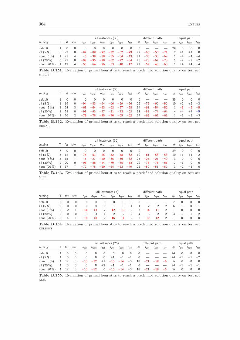
364 Tables
all instances (30) different path equal path
setting T fst slw ngm nsgm ntot tgm tsgm ttot # tgm tsgm ttot # tgm tsgm ttot
default 1 0 0 0 0 0 0 0 0 0 — — — 29 0 0 0
all (5 %) 0 23 0 −97 −89 −92 −72 −62 −79 27 −66 −55 −71 2 +1 +1 0
none (5 %) 1 21 4 −6 −39 −88 −35 −34 −43 27 −33 −33 −62 1 −4 −4 −4
all (20 %) 0 25 0 −99 −95 −98 −82 −72 −84 28 −78 −67 −78 1 −2 −2 −2
none (20 %) 1 19 4 −50 −64 −96 −53 −48 −47 27 −52 −48 −68 1 +4 +4 +4
Table B.151. Evaluation of primal heuristics to reach a predefined solution quality on test setmiplib.
all instances (38) different path equal path
setting T fst slw ngm nsgm ntot tgm tsgm ttot # tgm tsgm ttot # tgm tsgm ttot
default 3 0 0 0 0 0 0 0 0 0 — — — 35 0 0 0
all (5 %) 1 19 0 −94 −83 −94 −66 −59 −56 25 −75 −66 −56 10 +2 +2 +3
none (5 %) 1 24 3 −63 −64 −93 −63 −57 −58 34 −61 −54 −56 1 −5 −5 −5
all (20 %) 1 28 0 −98 −93 −97 −81 −73 −62 31 −83 −74 −64 4 +4 +4 +5
none (20 %) 1 26 2 −79 −78 −95 −70 −65 −62 34 −68 −62 −63 1 −3 −3 −3
Table B.152. Evaluation of primal heuristics to reach a predefined solution quality on test setcoral.
all instances (36) different path equal path
setting T fst slw ngm nsgm ntot tgm tsgm ttot # tgm tsgm ttot # tgm tsgm ttot
default 7 0 0 0 0 0 0 0 0 0 — — — 29 0 0 0
all (5 %) 5 12 0 −74 −51 −25 −52 −48 −32 19 −61 −58 −53 10 +1 +1 +2
none (5 %) 5 15 7 −5 −27 −40 −35 −36 −32 25 −25 −27 −40 3 0 0 0
all (20 %) 2 20 0 −95 −88 −44 −79 −75 −63 22 −78 −75 −65 7 −1 0 0
none (20 %) 3 17 7 −72 −75 −50 −64 −62 −49 25 −50 −51 −52 3 −2 −1 0
Table B.153. Evaluation of primal heuristics to reach a predefined solution quality on test setmilp.
all instances (7) different path equal path
setting T fst slw ngm nsgm ntot tgm tsgm ttot # tgm tsgm ttot # tgm tsgm ttot
default 0 0 0 0 0 0 0 0 0 0 — — — 7 0 0 0
all (5 %) 0 0 0 0 0 0 +1 0 −1 1 −2 −2 −2 6 +1 0 −1
none (5 %) 0 2 1 −14 −13 −2 −12 −10 −2 6 −14 −11 −2 1 0 0 0
all (20 %) 0 0 0 −3 −3 −1 −2 −2 −2 4 −3 −2 −2 3 −1 −1 −2
none (20 %) 0 4 1 −18 −18 −2 −16 −11 −2 6 −19 −12 −2 1 0 0 0
Table B.154. Evaluation of primal heuristics to reach a predefined solution quality on test setenlight.
all instances (25) different path equal path
setting T fst slw ngm nsgm ntot tgm tsgm ttot # tgm tsgm ttot # tgm tsgm ttot
default 1 0 0 0 0 0 0 0 0 0 — — — 24 0 0 0
all (5 %) 1 0 0 0 0 0 +1 +1 +1 0 — — — 24 +1 +1 +2
none (5 %) 1 12 3 −10 −12 +1 −15 −14 −3 18 −21 −18 −6 6 0 0 0
all (20 %) 1 0 0 0 0 +2 −1 −1 −1 0 — — — 24 −1 −1 −1
none (20 %) 1 12 3 −10 −12 0 −15 −14 −3 18 −21 −18 −6 6 0 0 0
Table B.155. Evaluation of primal heuristics to reach a predefined solution quality on test setalu.

Tables 365
all instances (16) different path equal path
setting T fst slw ngm nsgm ntot tgm tsgm ttot # tgm tsgm ttot # tgm tsgm ttot
default 0 0 0 0 0 0 0 0 0 0 — — — 16 0 0 0
all (5 %) 0 12 0 −96 −82 −90 −62 −65 −83 14 −67 −67 −83 2 0 0 0
none (5 %) 0 9 4 +23 −25 −78 −40 −56 −80 13 −47 −59 −80 3 0 0 0
all (20 %) 0 12 0 −100 −100 −100 −89 −95 −98 16 −89 −95 −98 0 — — —
none (20 %) 0 9 4 −22 −54 −90 −54 −70 −89 13 −62 −73 −89 3 0 0 0
Table B.156. Evaluation of primal heuristics to reach a predefined solution quality on test setfctp.
all instances (7) different path
setting T fst slw ngm nsgm ntot tgm tsgm ttot # tgm tsgm ttot
default 0 0 0 0 0 0 0 0 0 0 — — —
all (5 %) 0 0 0 0 0 0 +1 +1 +1 0 — — —
none (5 %) 0 2 5 +957 +151 +427 +40 +34 +45 7 +40 +34 +45
all (20 %) 0 0 0 0 0 0 −3 −3 −3 0 — — —
none (20 %) 0 2 5 +957 +151 +427 +44 +37 +49 7 +44 +37 +49
Table B.157. Evaluation of primal heuristics to reach a predefined solution quality on test setacc.
all instances (20) different path
setting T fst slw ngm nsgm ntot tgm tsgm ttot # tgm tsgm ttot
default 0 0 0 0 0 0 0 0 0 0 — — —
all (5 %) 0 17 0 −90 −69 −70 −29 −29 −33 20 −29 −29 −33
none (5 %) 0 1 19 +1316 +571 +372 +54 +51 +58 20 +54 +51 +58
all (20 %) 0 20 0 −99 −100 −100 −49 −52 −58 20 −49 −52 −58
none (20 %) 0 2 18 +1234 +531 +313 +48 +43 +44 20 +48 +43 +44
Table B.158. Evaluation of primal heuristics to reach a predefined solution quality on test set fc.
all instances (23) different path
setting T fst slw ngm nsgm ntot tgm tsgm ttot # tgm tsgm ttot
default 0 0 0 0 0 0 0 0 0 0 — — —
all (5 %) 0 23 0 −100 −97 −87 −86 −77 −68 23 −86 −77 −68
none (5 %) 0 20 0 −75 −73 −64 −62 −57 −67 23 −62 −57 −67
all (20 %) 0 23 0 −100 −100 −100 −95 −89 −88 23 −95 −89 −88
none (20 %) 0 20 0 −85 −82 −77 −66 −62 −76 23 −66 −62 −76
Table B.159. Evaluation of primal heuristics to reach a predefined solution quality on test setarcset.
all instances (41) different path
setting T fst slw ngm nsgm ntot tgm tsgm ttot # tgm tsgm ttot
default 0 0 0 0 0 0 0 0 0 0 — — —
all (5 %) 0 41 0 −100 −100 −100 −97 −96 −98 41 −97 −96 −98
none (5 %) 0 27 9 −57 −57 −73 −40 −41 −58 41 −40 −41 −58
all (20 %) 0 41 0 −100 −100 −100 −98 −98 −99 41 −98 −98 −99
none (20 %) 0 36 4 −80 −80 −85 −69 −67 −78 41 −69 −67 −78
Table B.160. Evaluation of primal heuristics to reach a predefined solution quality on test setmik.
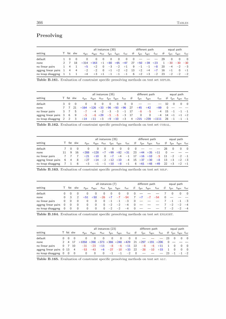
366 Tables
Presolving
all instances (30) different path equal path
setting T fst slw ngm nsgm ntot tgm tsgm ttot # tgm tsgm ttot # tgm tsgm ttot
default 1 0 0 0 0 0 0 0 0 0 — — — 29 0 0 0
none 2 7 18 +314 +163 +1 +80 +65 +47 27 +50 +39 +23 1 −30 −30 −30
no linear pairs 1 4 1 +5 +2 0 −3 −2 +1 9 −1 −1 +8 20 −4 −2 −3
aggreg linear pairs 1 4 4 −2 −2 0 +1 +2 +2 13 +2 +4 +7 16 +1 0 +1
no knap disaggreg 1 1 1 +4 +3 +1 −1 −1 −1 6 +2 +3 −2 23 −2 −2 −2
Table B.161. Evaluation of constraint specific presolving methods on test set miplib.
all instances (35) different path equal path
setting T fst slw ngm nsgm ntot tgm tsgm ttot # tgm tsgm ttot # tgm tsgm ttot
default 3 0 0 0 0 0 0 0 0 0 — — — 32 0 0 0
none 7 7 21 +164 +126 +33 +96 +93 +96 27 +45 +42 +69 0 — — —
no linear pairs 3 7 5 −7 −4 −2 −3 −3 −1 17 −6 −5 −4 15 −1 −1 −1
aggreg linear pairs 3 6 9 −5 −6 +29 −5 −5 −3 17 0 0 −4 14 +1 +1 +2
no knap disaggreg 2 2 3 +14 +11 +3 +9 +10 +3 4 +215 +239 +1111 28 −1 −1 −1
Table B.162. Evaluation of constraint specific presolving methods on test set coral.
all instances (35) different path equal path
setting T fst slw ngm nsgm ntot tgm tsgm ttot # tgm tsgm ttot # tgm tsgm ttot
default 7 0 0 0 0 0 0 0 0 0 — — — 28 0 0 0
none 11 9 16 +288 +128 +7 +99 +82 +31 23 +44 +35 +11 0 — — —
no linear pairs 7 7 7 +21 +10 0 +7 +4 −1 17 +16 +10 −5 11 −2 −2 −1
aggreg linear pairs 6 4 8 +27 +14 −2 +12 +10 −4 15 +37 +30 +8 13 +3 +2 +3
no knap disaggreg 7 1 6 +3 +1 −1 +10 +8 +1 6 +61 +48 +49 22 +3 +2 +1
Table B.163. Evaluation of constraint specific presolving methods on test set milp.
all instances (7) different path equal path
setting T fst slw ngm nsgm ntot tgm tsgm ttot # tgm tsgm ttot # tgm tsgm ttot
default 0 0 0 0 0 0 0 0 0 0 — — — 7 0 0 0
none 0 3 2 +51 +50 −26 +7 −7 −54 7 +7 −7 −54 0 — — —
no linear pairs 0 0 0 0 0 0 −1 −1 −3 0 — — — 7 −1 −1 −3
aggreg linear pairs 0 0 0 0 0 0 −2 −2 −4 0 — — — 7 −2 −2 −4
no knap disaggreg 0 0 0 0 0 0 −2 −2 −4 0 — — — 7 −2 −2 −4
Table B.164. Evaluation of constraint specific presolving methods on test set enlight.
all instances (23) different path equal path
setting T fst slw ngm nsgm ntot tgm tsgm ttot # tgm tsgm ttot # tgm tsgm ttot
default 0 0 0 0 0 0 0 0 0 0 — — — 23 0 0 0
none 2 4 17 +1058 +398 +373 +366 +248 +429 21 +297 +191 +206 0 — — —
no linear pairs 0 7 10 −31 −23 +13 −8 −6 +11 22 −8 −6 +11 1 0 0 0
aggreg linear pairs 0 13 4 −53 −43 +6 −27 −10 +33 22 −28 −10 +33 1 0 0 0
no knap disaggreg 0 0 0 0 0 0 −1 −1 −2 0 — — — 23 −1 −1 −2
Table B.165. Evaluation of constraint specific presolving methods on test set alu.
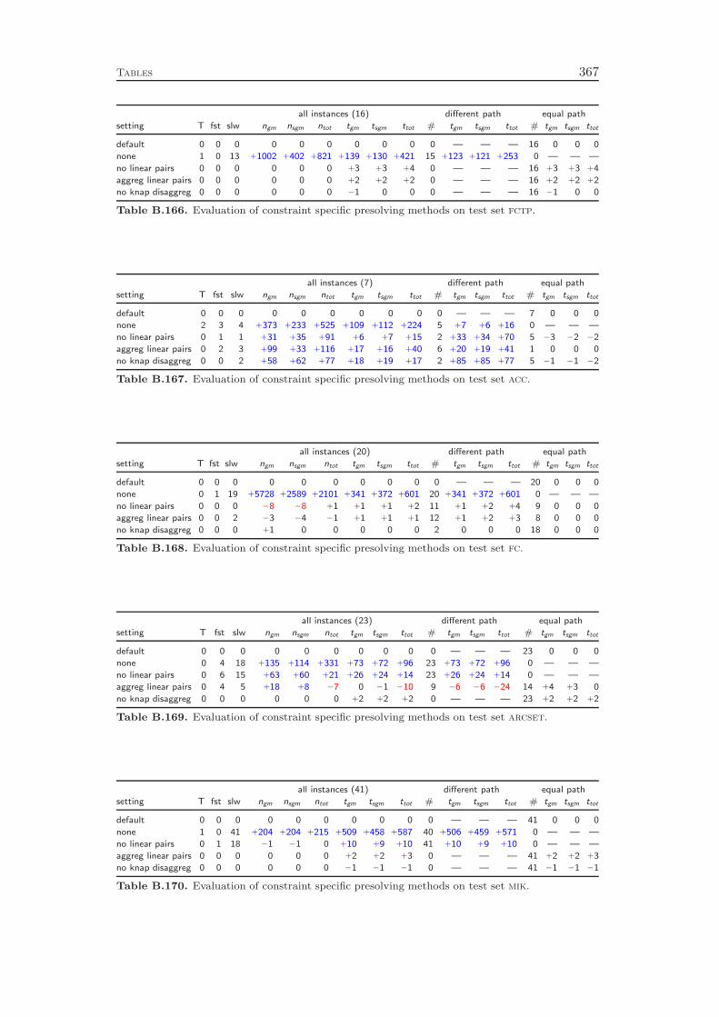
Tables 367
all instances (16) different path equal path
setting T fst slw ngm nsgm ntot tgm tsgm ttot # tgm tsgm ttot # tgm tsgm ttot
default 0 0 0 0 0 0 0 0 0 0 — — — 16 0 0 0
none 1 0 13 +1002 +402 +821 +139 +130 +421 15 +123 +121 +253 0 — — —
no linear pairs 0 0 0 0 0 0 +3 +3 +4 0 — — — 16 +3 +3 +4
aggreg linear pairs 0 0 0 0 0 0 +2 +2 +2 0 — — — 16 +2 +2 +2
no knap disaggreg 0 0 0 0 0 0 −1 0 0 0 — — — 16 −1 0 0
Table B.166. Evaluation of constraint specific presolving methods on test set fctp.
all instances (7) different path equal path
setting T fst slw ngm nsgm ntot tgm tsgm ttot # tgm tsgm ttot # tgm tsgm ttot
default 0 0 0 0 0 0 0 0 0 0 — — — 7 0 0 0
none 2 3 4 +373 +233 +525 +109 +112 +224 5 +7 +6 +16 0 — — —
no linear pairs 0 1 1 +31 +35 +91 +6 +7 +15 2 +33 +34 +70 5 −3 −2 −2
aggreg linear pairs 0 2 3 +99 +33 +116 +17 +16 +40 6 +20 +19 +41 1 0 0 0
no knap disaggreg 0 0 2 +58 +62 +77 +18 +19 +17 2 +85 +85 +77 5 −1 −1 −2
Table B.167. Evaluation of constraint specific presolving methods on test set acc.
all instances (20) different path equal path
setting T fst slw ngm nsgm ntot tgm tsgm ttot # tgm tsgm ttot # tgm tsgm ttot
default 0 0 0 0 0 0 0 0 0 0 — — — 20 0 0 0
none 0 1 19 +5728 +2589 +2101 +341 +372 +601 20 +341 +372 +601 0 — — —
no linear pairs 0 0 0 −8 −8 +1 +1 +1 +2 11 +1 +2 +4 9 0 0 0
aggreg linear pairs 0 0 2 −3 −4 −1 +1 +1 +1 12 +1 +2 +3 8 0 0 0
no knap disaggreg 0 0 0 +1 0 0 0 0 0 2 0 0 0 18 0 0 0
Table B.168. Evaluation of constraint specific presolving methods on test set fc.
all instances (23) different path equal path
setting T fst slw ngm nsgm ntot tgm tsgm ttot # tgm tsgm ttot # tgm tsgm ttot
default 0 0 0 0 0 0 0 0 0 0 — — — 23 0 0 0
none 0 4 18 +135 +114 +331 +73 +72 +96 23 +73 +72 +96 0 — — —
no linear pairs 0 6 15 +63 +60 +21 +26 +24 +14 23 +26 +24 +14 0 — — —
aggreg linear pairs 0 4 5 +18 +8 −7 0 −1 −10 9 −6 −6 −24 14 +4 +3 0
no knap disaggreg 0 0 0 0 0 0 +2 +2 +2 0 — — — 23 +2 +2 +2
Table B.169. Evaluation of constraint specific presolving methods on test set arcset.
all instances (41) different path equal path
setting T fst slw ngm nsgm ntot tgm tsgm ttot # tgm tsgm ttot # tgm tsgm ttot
default 0 0 0 0 0 0 0 0 0 0 — — — 41 0 0 0
none 1 0 41 +204 +204 +215 +509 +458 +587 40 +506 +459 +571 0 — — —
no linear pairs 0 1 18 −1 −1 0 +10 +9 +10 41 +10 +9 +10 0 — — —
aggreg linear pairs 0 0 0 0 0 0 +2 +2 +3 0 — — — 41 +2 +2 +3
no knap disaggreg 0 0 0 0 0 0 −1 −1 −1 0 — — — 41 −1 −1 −1
Table B.170. Evaluation of constraint specific presolving methods on test set mik.
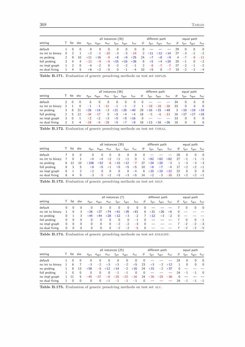
368 Tables
all instances (30) different path equal path
setting T fst slw ngm nsgm ntot tgm tsgm ttot # tgm tsgm ttot # tgm tsgm ttot
default 1 0 0 0 0 0 0 0 0 0 — — — 29 0 0 0
no int to binary 0 2 1 +2 −1 −10 −3 −3 −14 2 +11 +12 +14 27 −3 −2 −2
no probing 2 9 10 +11 +16 −9 +8 +9 +25 24 +7 +8 +9 4 −7 −9 −11
full probing 2 4 4 −12 −9 −9 +15 +16 +38 8 +5 +4 +20 20 −1 0 −2
no impl graph 1 2 0 −4 −2 0 −2 −2 −1 2 −8 −7 −7 27 −2 −1 −2
no dual fixing 1 4 5 +6 +2 −9 0 −1 −4 10 +5 0 −7 19 −2 −2 −4
Table B.171. Evaluation of generic presolving methods on test set miplib.
all instances (36) different path equal path
setting T fst slw ngm nsgm ntot tgm tsgm ttot # tgm tsgm ttot # tgm tsgm ttot
default 2 0 0 0 0 0 0 0 0 0 — — — 34 0 0 0
no int to binary 2 1 0 −1 −1 −11 −1 −1 −2 1 −18 −18 −18 33 0 0 0
no probing 3 8 21 +26 +14 +3 +21 +20 +40 29 +16 +15 +49 3 +19 +19 +19
full probing 2 5 12 −34 −17 0 +5 +4 +4 18 −5 −6 −13 16 +17 +17 +19
no impl graph 3 0 1 +2 +2 +3 +5 +5 +16 0 — — — 33 0 0 0
no dual fixing 2 3 4 −18 −6 −28 +5 +7 +8 16 +13 +16 +26 18 0 0 0
Table B.172. Evaluation of generic presolving methods on test set coral.
all instances (35) different path equal path
setting T fst slw ngm nsgm ntot tgm tsgm ttot # tgm tsgm ttot # tgm tsgm ttot
default 7 0 0 0 0 0 0 0 0 0 — — — 28 0 0 0
no int to binary 7 0 1 +4 +4 +2 +1 +1 0 1 +62 +62 +62 27 −1 −1 −1
no probing 6 12 10 +108 +52 −6 +15 +12 −7 27 +24 +20 −3 1 −3 −3 −3
full probing 8 3 5 +9 +5 +1 +5 +5 +5 10 +6 +7 −4 17 +2 +2 +1
no impl graph 6 1 2 +2 0 0 0 0 −4 6 +10 +10 +12 22 0 0 0
no dual fixing 8 4 9 −3 −5 +2 +5 +3 +5 14 +2 −3 −18 13 +2 +2 +1
Table B.173. Evaluation of generic presolving methods on test set milp.
all instances (7) different path equal path
setting T fst slw ngm nsgm ntot tgm tsgm ttot # tgm tsgm ttot # tgm tsgm ttot
default 0 0 0 0 0 0 0 0 0 0 — — — 7 0 0 0
no int to binary 1 0 3 +26 +27 +74 +41 +35 +81 6 +31 +26 +6 0 — — —
no probing 0 1 3 +44 +44 +28 +12 +3 −2 7 +12 +3 −2 0 — — —
full probing 0 0 0 0 0 0 0 0 −1 0 — — — 7 0 0 −1
no impl graph 0 0 0 0 0 0 −2 −2 −3 0 — — — 7 −2 −2 −3
no dual fixing 0 0 0 0 0 0 −2 −2 −5 0 — — — 7 −2 −2 −5
Table B.174. Evaluation of generic presolving methods on test set enlight.
all instances (25) different path equal path
setting T fst slw ngm nsgm ntot tgm tsgm ttot # tgm tsgm ttot # tgm tsgm ttot
default 1 0 0 0 0 0 0 0 0 0 — — — 24 0 0 0
no int to binary 1 6 7 −3 −2 +3 +3 −2 +5 23 +3 −2 +12 1 0 0 0
no probing 1 8 13 +58 −8 +12 +14 −2 +16 24 +15 −2 +37 0 — — —
full probing 1 0 0 0 0 0 −1 −1 0 0 — — — 24 −1 −1 0
no impl graph 1 11 5 −45 −37 −8 −25 −22 −16 24 −26 −25 −36 0 — — —
no dual fixing 1 0 0 0 0 +1 −1 −1 −1 0 — — — 24 −1 −1 −1
Table B.175. Evaluation of generic presolving methods on test set alu.

Tables 369
all instances (16) different path equal path
setting T fst slw ngm nsgm ntot tgm tsgm ttot # tgm tsgm ttot # tgm tsgm ttot
default 0 0 0 0 0 0 0 0 0 0 — — — 16 0 0 0
no int to binary 0 0 0 0 0 0 0 0 0 0 — — — 16 0 0 0
no probing 0 2 2 −3 −6 −3 −3 −4 −3 11 −4 −5 −3 5 0 0 0
full probing 0 2 1 −1 −1 −1 +1 0 +3 8 +1 0 +3 8 +1 +2 +2
no impl graph 0 0 0 0 0 0 +2 +2 +3 0 — — — 16 +2 +2 +3
no dual fixing 0 0 0 0 0 0 0 0 0 0 — — — 16 0 0 0
Table B.176. Evaluation of generic presolving methods on test set fctp.
all instances (7) different path equal path
setting T fst slw ngm nsgm ntot tgm tsgm ttot # tgm tsgm ttot # tgm tsgm ttot
default 0 0 0 0 0 0 0 0 0 0 — — — 7 0 0 0
no int to binary 0 0 0 0 0 0 +1 +1 +1 0 — — — 7 +1 +1 +1
no probing 3 1 3 +212 +286 +940 +95 +100 +268 1 −67 −67 −67 3 −3 −3 −3
full probing 0 0 2 +265 +32 +7 +41 +36 +4 3 +129 +139 +195 4 −2 −2 −2
no impl graph 0 0 0 0 0 0 +1 +1 +2 0 — — — 7 +1 +1 +2
no dual fixing 0 0 0 0 0 0 0 0 0 0 — — — 7 0 0 0
Table B.177. Evaluation of generic presolving methods on test set acc.
all instances (20) different path
setting T fst slw ngm nsgm ntot tgm tsgm ttot # tgm tsgm ttot
default 0 0 0 0 0 0 0 0 0 0 — — —
no int to binary 0 0 0 0 0 0 0 0 0 0 — — —
no probing 0 3 7 +13 +15 +29 +7 +9 +10 20 +7 +9 +10
full probing 0 0 0 0 0 0 0 0 0 0 — — —
no impl graph 0 0 0 0 0 0 0 0 0 0 — — —
no dual fixing 0 5 8 +9 +10 0 +7 +4 +2 20 +7 +4 +2
Table B.178. Evaluation of generic presolving methods on test set fc.
all instances (23) different path
setting T fst slw ngm nsgm ntot tgm tsgm ttot # tgm tsgm ttot
default 0 0 0 0 0 0 0 0 0 0 — — —
no int to binary 0 0 3 +6 +5 +2 +8 +7 +6 4 +26 +26 +30
no probing 0 5 7 +27 +13 +3 −3 −3 −12 14 −5 −5 −24
full probing 0 4 6 +19 +7 −14 +4 +2 −12 12 +5 +2 −30
no impl graph 0 0 0 0 0 0 +1 +1 +1 0 — — —
no dual fixing 0 9 10 +23 +11 +6 +7 +7 −5 23 +7 +7 −5
Table B.179. Evaluation of generic presolving methods on test set arcset.
all instances (41) different path equal path
setting T fst slw ngm nsgm ntot tgm tsgm ttot # tgm tsgm ttot # tgm tsgm ttot
default 0 0 0 0 0 0 0 0 0 0 — — — 41 0 0 0
no int to binary 0 11 5 −2 −2 +1 −4 −3 −1 26 −6 −4 −1 15 −2 −1 −1
no probing 0 6 25 +44 +44 +15 +34 +28 +16 41 +34 +28 +16 0 — — —
full probing 0 0 0 0 0 0 +3 +3 +2 0 — — — 41 +3 +3 +2
no impl graph 0 0 0 0 0 0 0 0 0 0 — — — 41 0 0 0
no dual fixing 0 0 0 0 0 0 +2 +2 +3 1 +8 +8 +8 40 +2 +2 +3
Table B.180. Evaluation of generic presolving methods on test set mik.
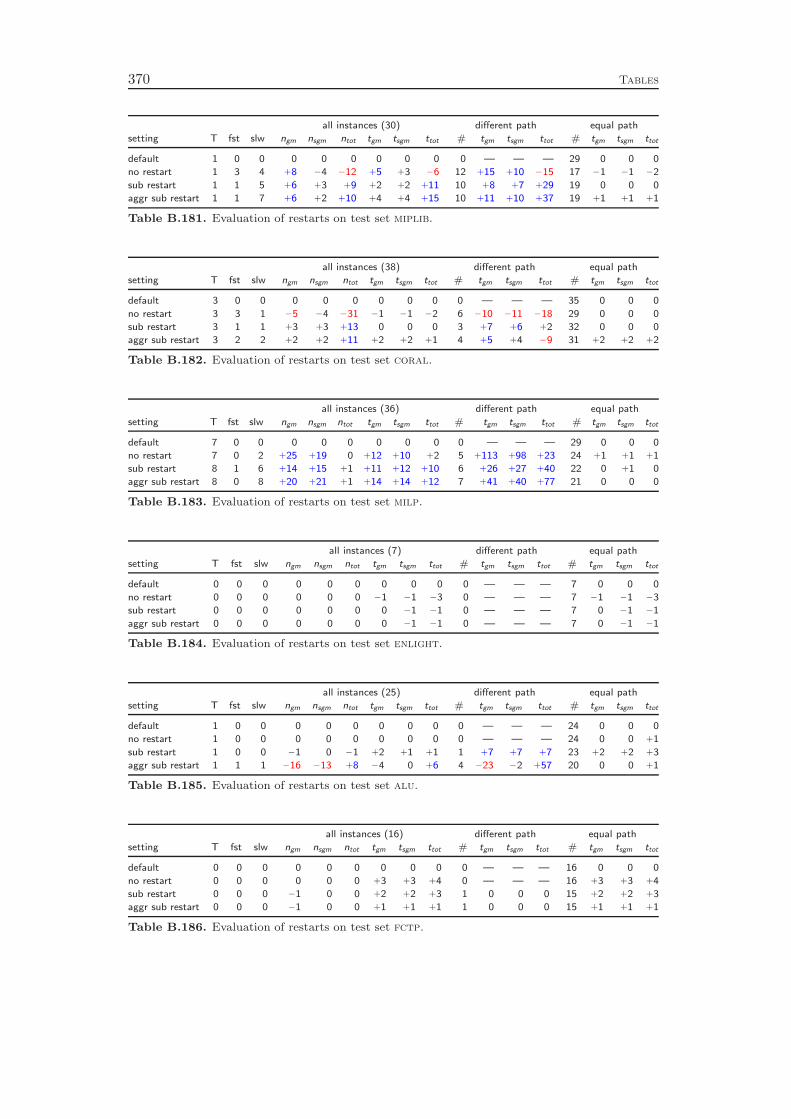
370 Tables
all instances (30) different path equal path
setting T fst slw ngm nsgm ntot tgm tsgm ttot # tgm tsgm ttot # tgm tsgm ttot
default 1 0 0 0 0 0 0 0 0 0 — — — 29 0 0 0
no restart 1 3 4 +8 −4 −12 +5 +3 −6 12 +15 +10 −15 17 −1 −1 −2
sub restart 1 1 5 +6 +3 +9 +2 +2 +11 10 +8 +7 +29 19 0 0 0
aggr sub restart 1 1 7 +6 +2 +10 +4 +4 +15 10 +11 +10 +37 19 +1 +1 +1
Table B.181. Evaluation of restarts on test set miplib.
all instances (38) different path equal path
setting T fst slw ngm nsgm ntot tgm tsgm ttot # tgm tsgm ttot # tgm tsgm ttot
default 3 0 0 0 0 0 0 0 0 0 — — — 35 0 0 0
no restart 3 3 1 −5 −4 −31 −1 −1 −2 6 −10 −11 −18 29 0 0 0
sub restart 3 1 1 +3 +3 +13 0 0 0 3 +7 +6 +2 32 0 0 0
aggr sub restart 3 2 2 +2 +2 +11 +2 +2 +1 4 +5 +4 −9 31 +2 +2 +2
Table B.182. Evaluation of restarts on test set coral.
all instances (36) different path equal path
setting T fst slw ngm nsgm ntot tgm tsgm ttot # tgm tsgm ttot # tgm tsgm ttot
default 7 0 0 0 0 0 0 0 0 0 — — — 29 0 0 0
no restart 7 0 2 +25 +19 0 +12 +10 +2 5 +113 +98 +23 24 +1 +1 +1
sub restart 8 1 6 +14 +15 +1 +11 +12 +10 6 +26 +27 +40 22 0 +1 0
aggr sub restart 8 0 8 +20 +21 +1 +14 +14 +12 7 +41 +40 +77 21 0 0 0
Table B.183. Evaluation of restarts on test set milp.
all instances (7) different path equal path
setting T fst slw ngm nsgm ntot tgm tsgm ttot # tgm tsgm ttot # tgm tsgm ttot
default 0 0 0 0 0 0 0 0 0 0 — — — 7 0 0 0
no restart 0 0 0 0 0 0 −1 −1 −3 0 — — — 7 −1 −1 −3
sub restart 0 0 0 0 0 0 0 −1 −1 0 — — — 7 0 −1 −1
aggr sub restart 0 0 0 0 0 0 0 −1 −1 0 — — — 7 0 −1 −1
Table B.184. Evaluation of restarts on test set enlight.
all instances (25) different path equal path
setting T fst slw ngm nsgm ntot tgm tsgm ttot # tgm tsgm ttot # tgm tsgm ttot
default 1 0 0 0 0 0 0 0 0 0 — — — 24 0 0 0
no restart 1 0 0 0 0 0 0 0 0 0 — — — 24 0 0 +1
sub restart 1 0 0 −1 0 −1 +2 +1 +1 1 +7 +7 +7 23 +2 +2 +3
aggr sub restart 1 1 1 −16 −13 +8 −4 0 +6 4 −23 −2 +57 20 0 0 +1
Table B.185. Evaluation of restarts on test set alu.
all instances (16) different path equal path
setting T fst slw ngm nsgm ntot tgm tsgm ttot # tgm tsgm ttot # tgm tsgm ttot
default 0 0 0 0 0 0 0 0 0 0 — — — 16 0 0 0
no restart 0 0 0 0 0 0 +3 +3 +4 0 — — — 16 +3 +3 +4
sub restart 0 0 0 −1 0 0 +2 +2 +3 1 0 0 0 15 +2 +2 +3
aggr sub restart 0 0 0 −1 0 0 +1 +1 +1 1 0 0 0 15 +1 +1 +1
Table B.186. Evaluation of restarts on test set fctp.

Tables 371
all instances (7) different path equal path
setting T fst slw ngm nsgm ntot tgm tsgm ttot # tgm tsgm ttot # tgm tsgm ttot
default 0 0 0 0 0 0 0 0 0 0 — — — 7 0 0 0
no restart 0 0 1 0 0 0 +3 +3 +4 0 — — — 7 +3 +3 +4
sub restart 0 0 0 0 0 0 −2 −1 −1 0 — — — 7 −2 −1 −1
aggr sub restart 0 0 0 0 0 0 +1 +1 +1 0 — — — 7 +1 +1 +1
Table B.187. Evaluation of restarts on test set acc.
all instances (20) different path equal path
setting T fst slw ngm nsgm ntot tgm tsgm ttot # tgm tsgm ttot # tgm tsgm ttot
default 0 0 0 0 0 0 0 0 0 0 — — — 20 0 0 0
no restart 0 3 2 +28 +8 +6 −1 +1 +4 12 −2 +2 +10 8 0 0 0
sub restart 0 0 1 −3 −2 0 +1 +1 +1 2 +11 +11 +12 18 0 0 0
aggr sub restart 0 0 2 −10 −8 −14 +3 +2 +1 5 +7 +3 −1 15 +2 +2 +2
Table B.188. Evaluation of restarts on test set fc.
all instances (23) different path equal path
setting T fst slw ngm nsgm ntot tgm tsgm ttot # tgm tsgm ttot # tgm tsgm ttot
default 0 0 0 0 0 0 0 0 0 0 — — — 23 0 0 0
no restart 0 0 1 +4 +4 +5 +10 +9 +6 1 +238 +238 +238 22 +4 +4 +4
sub restart 0 2 1 −8 −6 −7 −1 −1 +1 3 −27 −27 −40 20 +3 +3 +3
aggr sub restart 0 1 1 −5 −3 +1 0 +1 +2 4 −4 +1 +10 19 +1 +1 +1
Table B.189. Evaluation of restarts on test set arcset.
all instances (41) different path equal path
setting T fst slw ngm nsgm ntot tgm tsgm ttot # tgm tsgm ttot # tgm tsgm ttot
default 0 0 0 0 0 0 0 0 0 0 — — — 41 0 0 0
no restart 3 0 41 +311 +310 +403 +553 +500 +697 38 +533 +494 +604 0 — — —
sub restart 0 0 0 0 0 0 0 0 0 0 — — — 41 0 0 0
aggr sub restart 0 0 0 0 0 0 +2 +1 +1 0 — — — 41 +2 +1 +1
Table B.190. Evaluation of restarts on test set mik.

372 Tables
Conflict Analysis
all instances (30) different path equal path
setting T fst slw ngm nsgm ntot tgm tsgm ttot # tgm tsgm ttot # tgm tsgm ttot
default 1 0 0 0 0 0 0 0 0 0 — — — 29 0 0 0
prop 2 4 1 −7 −6 +7 −1 0 +15 13 −6 −5 −7 15 −2 −1 −1
prop/inflp 2 1 7 −1 −1 +14 +7 +6 +19 14 +4 +3 +1 14 +5 +2 0
prop/inflp/age 1 4 2 −9 −9 −33 0 0 +7 14 −2 −2 +1 14 −1 −1 −1
prop/lp 3 2 9 −15 −14 −22 +13 +12 +33 18 +13 +11 +14 9 +2 +2 +3
all 3 1 8 −11 −10 −19 +14 +14 +35 21 +14 +13 +20 6 −1 −1 −2
full 2 1 17 −15 −15 −27 +26 +24 +29 22 +33 +31 +42 6 +2 +1 +1
Table B.191. Evaluation of conflict analysis on test set miplib.
all instances (37) different path equal path
setting T fst slw ngm nsgm ntot tgm tsgm ttot # tgm tsgm ttot # tgm tsgm ttot
default 2 0 0 0 0 0 0 0 0 0 — — — 35 0 0 0
prop 1 10 3 −21 −20 −23 −10 −10 −8 21 −9 −8 +22 14 +3 +3 +2
prop/inflp 2 12 5 −16 −13 −21 −1 −1 +7 26 −3 −4 +3 8 0 0 0
prop/inflp/age 2 11 7 −31 −29 −48 −7 −7 0 26 −2 −3 +12 8 +3 +3 +2
prop/lp 3 11 8 −25 −22 −42 +3 +2 +19 30 −1 −2 +10 4 +1 +1 +2
all 2 9 16 −29 −27 −46 +3 +2 +8 32 +11 +10 +25 2 +2 +2 +2
full 2 5 21 −38 −36 −48 +9 +8 +15 32 +18 +17 +38 2 +2 +2 +2
Table B.192. Evaluation of conflict analysis on test set coral.
all instances (35) different path equal path
setting T fst slw ngm nsgm ntot tgm tsgm ttot # tgm tsgm ttot # tgm tsgm ttot
default 6 0 0 0 0 0 0 0 0 0 — — — 29 0 0 0
prop 4 2 2 −16 −16 −21 −13 −13 −11 11 −12 −12 −7 18 +1 +1 +2
prop/inflp 3 4 1 −29 −29 −35 −26 −26 −23 12 −14 −15 −14 17 0 0 0
prop/inflp/age 3 7 1 −35 −36 −40 −28 −28 −25 12 −19 −20 −18 17 +2 +2 +2
prop/lp 4 8 5 −47 −48 −51 −31 −31 −32 16 −21 −21 −33 12 +3 +2 +3
all 5 5 8 −44 −45 −46 −24 −24 −23 18 −6 −6 −18 10 +1 +1 +1
full 3 7 12 −46 −47 −58 −19 −18 −23 18 +16 +15 +12 10 −1 0 0
Table B.193. Evaluation of conflict analysis on test set milp.
all instances (7) different path equal path
setting T fst slw ngm nsgm ntot tgm tsgm ttot # tgm tsgm ttot # tgm tsgm ttot
default 0 0 0 0 0 0 0 0 0 0 — — — 7 0 0 0
prop 0 2 1 −30 −29 −25 −12 −11 −7 6 −14 −12 −7 1 0 0 0
prop/inflp 0 4 1 −49 −48 −53 −25 −21 −37 6 −29 −23 −37 1 0 0 0
prop/inflp/age 0 5 0 −79 −79 −96 −46 −49 −79 6 −51 −52 −79 1 0 0 0
prop/lp 0 4 1 −50 −49 −55 −24 −21 −38 6 −28 −23 −38 1 0 0 0
all 0 5 0 −50 −49 −63 −26 −26 −52 6 −30 −28 −52 1 0 0 0
full 0 5 0 −50 −49 −64 −26 −26 −53 6 −29 −28 −53 1 0 0 0
Table B.194. Evaluation of conflict analysis on test set enlight.
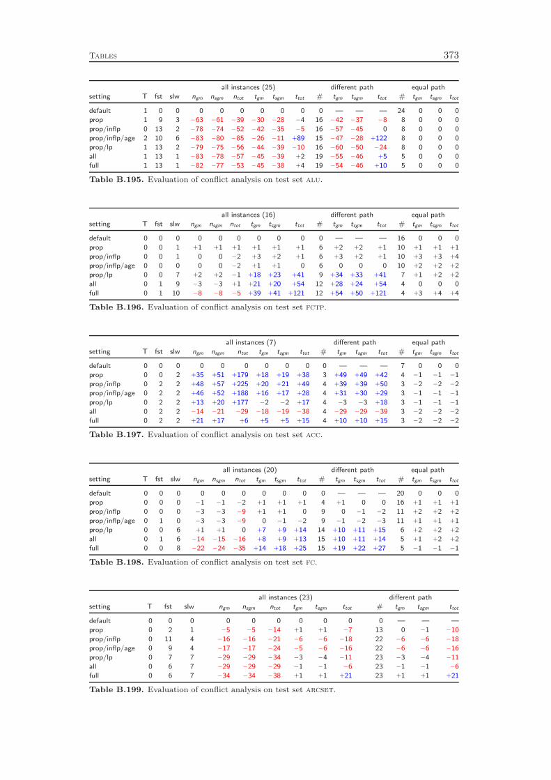
Tables 373
all instances (25) different path equal path
setting T fst slw ngm nsgm ntot tgm tsgm ttot # tgm tsgm ttot # tgm tsgm ttot
default 1 0 0 0 0 0 0 0 0 0 — — — 24 0 0 0
prop 1 9 3 −63 −61 −39 −30 −28 −4 16 −42 −37 −8 8 0 0 0
prop/inflp 0 13 2 −78 −74 −52 −42 −35 −5 16 −57 −45 0 8 0 0 0
prop/inflp/age 2 10 6 −83 −80 −85 −26 −11 +89 15 −47 −28 +122 8 0 0 0
prop/lp 1 13 2 −79 −75 −56 −44 −39 −10 16 −60 −50 −24 8 0 0 0
all 1 13 1 −83 −78 −57 −45 −39 +2 19 −55 −46 +5 5 0 0 0
full 1 13 1 −82 −77 −53 −45 −38 +4 19 −54 −46 +10 5 0 0 0
Table B.195. Evaluation of conflict analysis on test set alu.
all instances (16) different path equal path
setting T fst slw ngm nsgm ntot tgm tsgm ttot # tgm tsgm ttot # tgm tsgm ttot
default 0 0 0 0 0 0 0 0 0 0 — — — 16 0 0 0
prop 0 0 1 +1 +1 +1 +1 +1 +1 6 +2 +2 +1 10 +1 +1 +1
prop/inflp 0 0 1 0 0 −2 +3 +2 +1 6 +3 +2 +1 10 +3 +3 +4
prop/inflp/age 0 0 0 0 0 −2 +1 +1 0 6 0 0 0 10 +2 +2 +2
prop/lp 0 0 7 +2 +2 −1 +18 +23 +41 9 +34 +33 +41 7 +1 +2 +2
all 0 1 9 −3 −3 +1 +21 +20 +54 12 +28 +24 +54 4 0 0 0
full 0 1 10 −8 −8 −5 +39 +41 +121 12 +54 +50 +121 4 +3 +4 +4
Table B.196. Evaluation of conflict analysis on test set fctp.
all instances (7) different path equal path
setting T fst slw ngm nsgm ntot tgm tsgm ttot # tgm tsgm ttot # tgm tsgm ttot
default 0 0 0 0 0 0 0 0 0 0 — — — 7 0 0 0
prop 0 0 2 +35 +51 +179 +18 +19 +38 3 +49 +49 +42 4 −1 −1 −1
prop/inflp 0 2 2 +48 +57 +225 +20 +21 +49 4 +39 +39 +50 3 −2 −2 −2
prop/inflp/age 0 2 2 +46 +52 +188 +16 +17 +28 4 +31 +30 +29 3 −1 −1 −1
prop/lp 0 2 2 +13 +20 +177 −2 −2 +17 4 −3 −3 +18 3 −1 −1 −1
all 0 2 2 −14 −21 −29 −18 −19 −38 4 −29 −29 −39 3 −2 −2 −2
full 0 2 2 +21 +17 +6 +5 +5 +15 4 +10 +10 +15 3 −2 −2 −2
Table B.197. Evaluation of conflict analysis on test set acc.
all instances (20) different path equal path
setting T fst slw ngm nsgm ntot tgm tsgm ttot # tgm tsgm ttot # tgm tsgm ttot
default 0 0 0 0 0 0 0 0 0 0 — — — 20 0 0 0
prop 0 0 0 −1 −1 −2 +1 +1 +1 4 +1 0 0 16 +1 +1 +1
prop/inflp 0 0 0 −3 −3 −9 +1 +1 0 9 0 −1 −2 11 +2 +2 +2
prop/inflp/age 0 1 0 −3 −3 −9 0 −1 −2 9 −1 −2 −3 11 +1 +1 +1
prop/lp 0 0 6 +1 +1 0 +7 +9 +14 14 +10 +11 +15 6 +2 +2 +2
all 0 1 6 −14 −15 −16 +8 +9 +13 15 +10 +11 +14 5 +1 +2 +2
full 0 0 8 −22 −24 −35 +14 +18 +25 15 +19 +22 +27 5 −1 −1 −1
Table B.198. Evaluation of conflict analysis on test set fc.
all instances (23) different path
setting T fst slw ngm nsgm ntot tgm tsgm ttot # tgm tsgm ttot
default 0 0 0 0 0 0 0 0 0 0 — — —
prop 0 2 1 −5 −5 −14 +1 +1 −7 13 0 −1 −10
prop/inflp 0 11 4 −16 −16 −21 −6 −6 −18 22 −6 −6 −18
prop/inflp/age 0 9 4 −17 −17 −24 −5 −6 −16 22 −6 −6 −16
prop/lp 0 7 7 −29 −29 −34 −3 −4 −11 23 −3 −4 −11
all 0 6 7 −29 −29 −29 −1 −1 −6 23 −1 −1 −6
full 0 6 7 −34 −34 −38 +1 +1 +21 23 +1 +1 +21
Table B.199. Evaluation of conflict analysis on test set arcset.
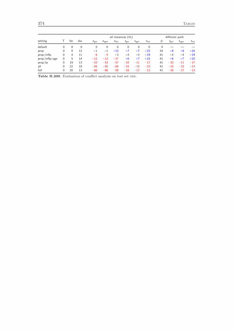
374 Tables
all instances (41) different path
setting T fst slw ngm nsgm ntot tgm tsgm ttot # tgm tsgm ttot
default 0 0 0 0 0 0 0 0 0 0 — — —
prop 0 0 12 +1 +1 +13 +7 +7 +22 34 +8 +8 +24
prop/inflp 0 4 11 −6 −5 +3 +4 +4 +19 41 +4 +4 +19
prop/inflp/age 0 5 14 −12 −12 −17 +6 +7 +15 41 +6 +7 +15
prop/lp 0 19 13 −53 −53 −57 −10 −11 −17 41 −10 −11 −17
all 0 22 10 −56 −55 −60 −15 −15 −23 41 −15 −15 −23
full 0 20 13 −60 −60 −59 −16 −17 −13 41 −16 −17 −13
Table B.200. Evaluation of conflict analysis on test set mik.

Tables 375
Comparison to Cplex
all instances (30) different path
setting T fst slw ngm nsgm ntot tgm tsgm ttot # tgm tsgm ttot
Cplex 10.0.1 1 0 0 0 0 0 0 0 0 0 — — —
SCIP 0.90f 1 5 25 −68 −38 −6 +131 +51 +1 28 +202 +94 +25
SCIP 0.90i 1 5 24 −62 −41 −21 +108 +44 −2 28 +164 +81 +12
Table B.201. Evaluation of Cplex 10.0.1, SCIP 0.90f, and SCIP 0.90i on test set miplib.
all instances (37) different path
setting T fst slw ngm nsgm ntot tgm tsgm ttot # tgm tsgm ttot
Cplex 10.0.1 4 0 0 0 0 0 0 0 0 0 — — —
SCIP 0.90f 3 8 27 +30 −1 +58 +237 +117 −1 30 +289 +147 +27
SCIP 0.90i 2 13 24 −35 −43 −66 +121 +54 −29 31 +196 +103 +3
Table B.202. Evaluation of Cplex 10.0.1, SCIP 0.90f, and SCIP 0.90i on test set coral.
all instances (36) different path
setting T fst slw ngm nsgm ntot tgm tsgm ttot # tgm tsgm ttot
Cplex 10.0.1 1 0 0 0 0 0 0 0 0 0 — — —
SCIP 0.90f 7 5 28 −5 +40 +220 +295 +256 +240 28 +183 +151 +152
SCIP 0.90i 3 9 25 −43 −20 +62 +176 +149 +115 32 +170 +143 +129
Table B.203. Evaluation of Cplex 10.0.1, SCIP 0.90f, and SCIP 0.90i on test set milp.
all instances (7) different path
setting T fst slw ngm nsgm ntot tgm tsgm ttot # tgm tsgm ttot
Cplex 10.0.1 1 0 0 0 0 0 0 0 0 0 — — —
SCIP 0.90f 0 1 4 −56 −26 −55 +9 −12 −49 6 +42 +20 +31
SCIP 0.90i 0 3 1 −97 −89 −98 −61 −73 −95 6 −43 −66 −94
Table B.204. Evaluation of Cplex 10.0.1, SCIP 0.90f, and SCIP 0.90i on test set enlight.
all instances (24) different path
setting T fst slw ngm nsgm ntot tgm tsgm ttot # tgm tsgm ttot
Cplex 10.0.1 1 0 0 0 0 0 0 0 0 0 — — —
SCIP 0.90f 0 9 12 −90 −70 −75 −14 −10 −64 23 −8 −1 −48
SCIP 0.90i 0 11 8 −99 −97 −97 −68 −63 −71 23 −59 −50 −45
Table B.205. Evaluation of Cplex 10.0.1, SCIP 0.90f, and SCIP 0.90i on test set alu.
all instances (16) different path
setting T fst slw ngm nsgm ntot tgm tsgm ttot # tgm tsgm ttot
Cplex 10.0.1 0 0 0 0 0 0 0 0 0 0 — — —
SCIP 0.90f 0 0 12 −1 +10 +1 +109 +82 +49 16 +109 +82 +49
SCIP 0.90i 0 0 12 −12 +11 +11 +90 +72 +50 16 +90 +72 +50
Table B.206. Evaluation of Cplex 10.0.1, SCIP 0.90f, and SCIP 0.90i on test set fctp.
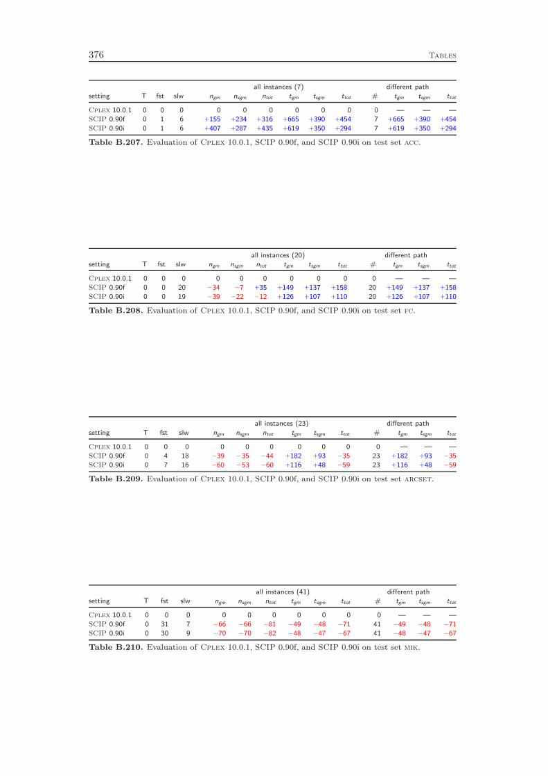
376 Tables
all instances (7) different path
setting T fst slw ngm nsgm ntot tgm tsgm ttot # tgm tsgm ttot
Cplex 10.0.1 0 0 0 0 0 0 0 0 0 0 — — —
SCIP 0.90f 0 1 6 +155 +234 +316 +665 +390 +454 7 +665 +390 +454
SCIP 0.90i 0 1 6 +407 +287 +435 +619 +350 +294 7 +619 +350 +294
Table B.207. Evaluation of Cplex 10.0.1, SCIP 0.90f, and SCIP 0.90i on test set acc.
all instances (20) different path
setting T fst slw ngm nsgm ntot tgm tsgm ttot # tgm tsgm ttot
Cplex 10.0.1 0 0 0 0 0 0 0 0 0 0 — — —
SCIP 0.90f 0 0 20 −34 −7 +35 +149 +137 +158 20 +149 +137 +158
SCIP 0.90i 0 0 19 −39 −22 −12 +126 +107 +110 20 +126 +107 +110
Table B.208. Evaluation of Cplex 10.0.1, SCIP 0.90f, and SCIP 0.90i on test set fc.
all instances (23) different path
setting T fst slw ngm nsgm ntot tgm tsgm ttot # tgm tsgm ttot
Cplex 10.0.1 0 0 0 0 0 0 0 0 0 0 — — —
SCIP 0.90f 0 4 18 −39 −35 −44 +182 +93 −35 23 +182 +93 −35
SCIP 0.90i 0 7 16 −60 −53 −60 +116 +48 −59 23 +116 +48 −59
Table B.209. Evaluation of Cplex 10.0.1, SCIP 0.90f, and SCIP 0.90i on test set arcset.
all instances (41) different path
setting T fst slw ngm nsgm ntot tgm tsgm ttot # tgm tsgm ttot
Cplex 10.0.1 0 0 0 0 0 0 0 0 0 0 — — —
SCIP 0.90f 0 31 7 −66 −66 −81 −49 −48 −71 41 −49 −48 −71
SCIP 0.90i 0 30 9 −70 −70 −82 −48 −47 −67 41 −48 −47 −67
Table B.210. Evaluation of Cplex 10.0.1, SCIP 0.90f, and SCIP 0.90i on test set mik.
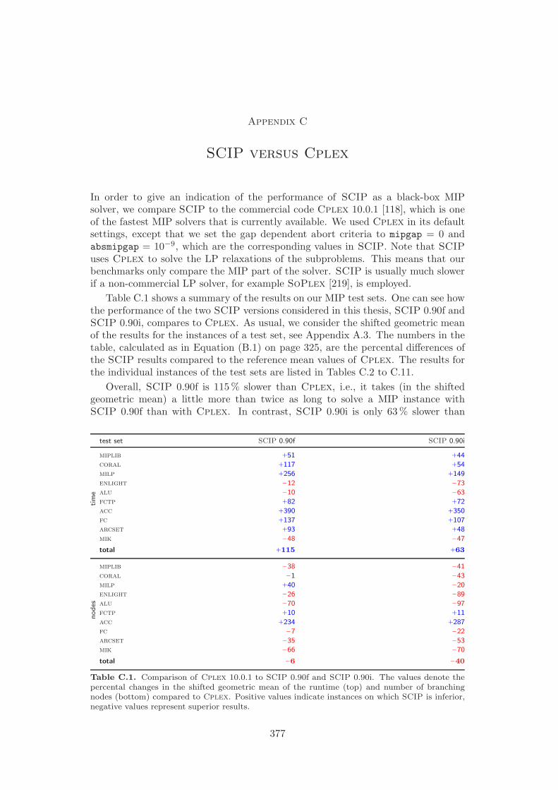
Appendix C
SCIP versus Cplex
In order to give an indication of the performance of SCIP as a black-box MIPsolver, we compare SCIP to the commercial code Cplex 10.0.1 [118], which is oneof the fastest MIP solvers that is currently available. We used Cplex in its defaultsettings, except that we set the gap dependent abort criteria to mipgap = 0 andabsmipgap = 10−9, which are the corresponding values in SCIP. Note that SCIPuses Cplex to solve the LP relaxations of the subproblems. This means that ourbenchmarks only compare the MIP part of the solver. SCIP is usually much slowerif a non-commercial LP solver, for example SoPlex [219], is employed.
Table C.1 shows a summary of the results on our MIP test sets. One can see howthe performance of the two SCIP versions considered in this thesis, SCIP 0.90f andSCIP 0.90i, compares to Cplex. As usual, we consider the shifted geometric meanof the results for the instances of a test set, see Appendix A.3. The numbers in thetable, calculated as in Equation (B.1) on page 325, are the percental differences ofthe SCIP results compared to the reference mean values of Cplex. The results forthe individual instances of the test sets are listed in Tables C.2 to C.11.
Overall, SCIP 0.90f is 115 % slower than Cplex, i.e., it takes (in the shiftedgeometric mean) a little more than twice as long to solve a MIP instance withSCIP 0.90f than with Cplex. In contrast, SCIP 0.90i is only 63 % slower than
test set SCIP 0.90f SCIP 0.90i
tim
e
miplib +51 +44
coral +117 +54
milp +256 +149
enlight −12 −73
alu −10 −63
fctp +82 +72
acc +390 +350
fc +137 +107
arcset +93 +48
mik −48 −47
total +115 +63
no
des
miplib −38 −41
coral −1 −43
milp +40 −20
enlight −26 −89
alu −70 −97
fctp +10 +11
acc +234 +287
fc −7 −22
arcset −35 −53
mik −66 −70
total −6 −40
Table C.1. Comparison of Cplex 10.0.1 to SCIP 0.90f and SCIP 0.90i. The values denote thepercental changes in the shifted geometric mean of the runtime (top) and number of branchingnodes (bottom) compared to Cplex. Positive values indicate instances on which SCIP is inferior,negative values represent superior results.
377

378 SCIP versus Cplex
Cplex 10.0.1 SCIP 0.90f SCIP 0.90i
Nodes Time Nodes Time Nodes Time
modglob 245 0.5 13 2.0 241 2.6
fiber 72 0.5 29 2.8 10 1.7
p2756 16 0.5 95 5.1 37 4.6
gesa2 39 0.5 3 5.9 8 5.6
set1ch 326 0.5 10 3.3 23 2.6
fixnet6 132 1.0 11 5.3 23 2.6
pp08a 618 1.1 1 196 3.0 1 20 2.9
vpm2 3 269 1.1 5 846 6.8 723 2.2
pp08aCUTS 1 372 2.0 817 3.7 426 2.8
10teams 22 4.4 1 374 43.1 538 39.8
gesa2-o 3 380 4.8 1 8.6 7 8.3
misc07 11 49 9.7 20 982 30.8 25 256 39.3
air05 288 12.4 291 124.8 342 90.9
air04 128 14.8 19 233.6 258 214.6
cap6000 4 565 15.8 3 165 8.6 3 65 8.8
nw04 126 20.1 7 73.1 5 77.7
aflow30a 11 832 30.5 2 180 33.8 2 426 30.2
qiu 2 371 31.6 10 567 185.4 8 697 110.0
mzzv42z 183 52.4 1 404 599.0 1 91 823.8
mod011 45 70.1 2 769 279.7 2 731 200.5
pk1 338 108 83.3 233 736 113.7 228 745 136.4
rout 41 345 91.8 12 542 55.0 28 669 79.1
mas76 660 320 122.5 414 423 142.3 347 197 134.9
disctom 50 195.2 1 98.8 1 94.7
mzzv11 1 873 219.0 1 786 1291.6 3 271 1148.3
harp2 1 71 588 1033.8 1 727 702 1415.0 >4 925 65 >3600.0
mas74 4 451 916 1267.3 4 86 233 2515.1 3 272 670 1477.8
noswot 4 717 721 1528.3 >5 203 78 >3600.0 983 43 2210.9
fast0507 13 997 3141.7 1 424 749.4 1 445 772.8
manna81 >1 177 281 >3600.0 1 4.6 2 5.6
geom. mean 2 556 20.7 818 47.8 963 43.1
sh. geom. mean 3 662 46.8 2 271 70.9 2 178 67.7
arithm. mean 417 142 385.2 391 56 388.1 327 901 377.7
Table C.2. Detailed benchmark results on the miplib test set. Values printed in red and blueindicate a difference of at least a factor of 2 to the reference Cplex results.
Cplex, which is an almost 25 % performance improvement with respect to the olderversion SCIP 0.90f. Thus, the conclusions we draw from our computational experi-ments and the resulting changes in the default settings indeed lead to a substantialenhancement in the MIP solving capabilities of SCIP. As a conclusion of the com-parison to Cplex, we take the results as evidence that the algorithms of SCIP areclose to the state-of-the-art in MIP solving, which substantiates the significance ofour computational experiments on SCIP.

SCIP versus Cplex 379
Cplex 10.0.1 SCIP 0.90f SCIP 0.90i
Nodes Time Nodes Time Nodes Time
neos-583731 1 0.5 2 71 134.8 185 63.2
neos-612125 2 0.9 215 67.6 341 55.7
neos-633273 1 1.1 4 48 1209.2 2 673 481.5
neos-612143 15 1.2 441 92.7 407 56.3
neos-494568 40 1.4 142 22.4 91 45.5
neos-584851 40 2.3 1 408 101.1 521 76.4
neos-717614 734 2.7 >932 392 >3600.0 174 879 710.1
neos-498623 80 3.7 79 38.4 306 54.9
neos-555001 470 4.7 140 7.0 1 4.1
neos-807639 5 90 7.0 16 284 150.6 13 650 147.6
neos-585467 973 9.9 347 23.2 189 17.0
neos-565815 8 11.3 3 26.9 1 41.7
aligninq 1 918 15.0 715 31.6 1 905 24.3
neos-570431 1 124 17.6 1 456 31.6 2 105 38.1
neos-504815 11 72 28.2 10 420 70.5 6 896 52.1
prod1 61 292 34.6 26 784 33.6 25 439 43.0
neos-738098 1 49.9 >199 >3600.0 >68 >3600.0
neos-480878 17 603 57.1 11 512 109.5 7 266 82.7
binkar10_1 7 992 63.4 205 358 844.6 259 288 974.3
neos-512201 21 202 69.5 15 772 179.2 10 720 131.1
neos-538916 55 938 72.6 40 693 113.7 12 731 61.2
neos-530627 823 990 77.6 2 405 10 1146.3 3 0.5
neos-796608 701 625 96.5 4 366 657 1691.7 — —
neos-538867 124 697 119.5 155 214 298.8 42 468 162.2
neos-791021 129 140.0 1 147.7 34 230.6
neos-686190 12 11 155.9 6 320 237.2 6 21 328.3
neos-506422 6 113 163.1 7 233 246.4 1 894 112.0
bienst1 7 918 219.6 12 24 339.0 12 473 55.8
prod2 276 396 299.3 107 299 207.3 69 191 173.9
neos-585192 28 262 476.1 1 690 69.5 903 62.4
neos-476283 3 710 587.8 1 66 1154.3 1 294 1209.1
neos-808072 53 464 1109.4 478 106.1 444 151.6
neos-787933 >20 469 >1967.8 1 102.6 1 99.7
neos-503737 50 438 2087.1 2 53 192.6 4 838 347.6
lrn 365 796 2742.3 >49 410 >3600.0 >66 579 >3600.0
bienst2 >109 661 >3600.0 113 376 1168.9 81 708 344.9
neos-551991 >8 19 >3600.0 3 444 496.4 6 542 785.2
neos-595925 >691 192 >3600.0 232 871 531.9 111 587 348.5
geom. mean 2 323 52.9 2 995 176.4 1 486 116.0
sh. geom. mean 4 720 88.2 4 608 189.3 2 659 134.7
arithm. mean 74 807 578.4 118 53 555.0 25 17 399.3
Table C.3. Detailed benchmark results on the coral test set. Values printed in red and blueindicate a difference of at least a factor of 2 to the reference Cplex results.
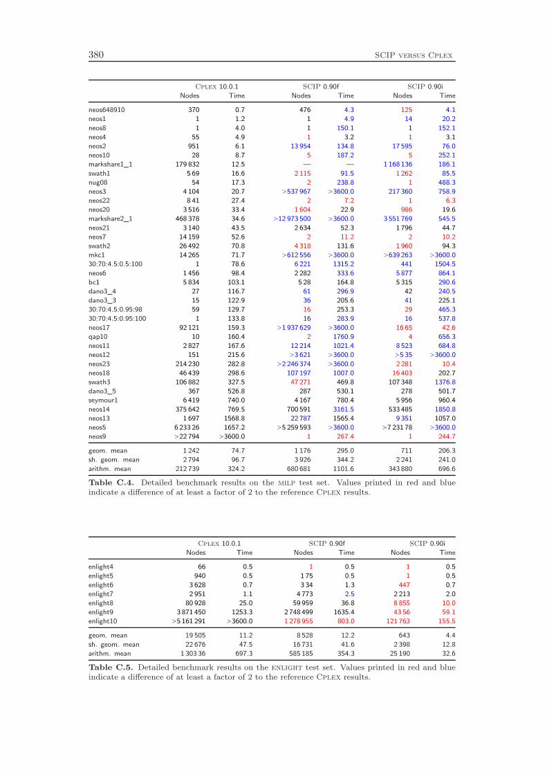
380 SCIP versus Cplex
Cplex 10.0.1 SCIP 0.90f SCIP 0.90i
Nodes Time Nodes Time Nodes Time
neos648910 370 0.7 476 4.3 125 4.1
neos1 1 1.2 1 4.9 14 20.2
neos8 1 4.0 1 150.1 1 152.1
neos4 55 4.9 1 3.2 1 3.1
neos2 951 6.1 13 954 134.8 17 595 76.0
neos10 28 8.7 5 187.2 5 252.1
markshare1_1 179 832 12.5 — — 1 168 136 186.1
swath1 5 69 16.6 2 115 91.5 1 262 85.5
nug08 54 17.3 2 238.8 1 488.3
neos3 4 104 20.7 >537 967 >3600.0 217 360 758.9
neos22 8 41 27.4 2 7.2 1 6.3
neos20 3 516 33.4 1 604 22.9 986 19.6
markshare2_1 468 378 34.6 >12 973 500 >3600.0 3 551 769 545.5
neos21 3 140 43.5 2 634 52.3 1 796 44.7
neos7 14 159 52.6 2 11.2 2 10.2
swath2 26 492 70.8 4 318 131.6 1 960 94.3
mkc1 14 265 71.7 >612 556 >3600.0 >639 263 >3600.0
30:70:4.5:0.5:100 1 78.6 6 221 1315.2 441 1504.5
neos6 1 456 98.4 2 282 333.6 5 877 864.1
bc1 5 834 103.1 5 28 164.8 5 315 290.6
dano3_4 27 116.7 61 296.9 42 240.5
dano3_3 15 122.9 36 205.6 41 225.1
30:70:4.5:0.95:98 59 129.7 16 253.3 29 465.3
30:70:4.5:0.95:100 1 133.8 16 283.9 16 537.8
neos17 92 121 159.3 >1 937 629 >3600.0 16 65 42.6
qap10 10 160.4 2 1760.9 4 656.3
neos11 2 827 167.6 12 214 1021.4 8 523 684.8
neos12 151 215.6 >3 621 >3600.0 >5 35 >3600.0
neos23 214 230 282.8 >2 246 374 >3600.0 2 281 10.4
neos18 46 439 298.6 107 197 1007.0 16 403 202.7
swath3 106 882 327.5 47 271 469.8 107 348 1376.8
dano3_5 367 526.8 287 530.1 278 501.7
seymour1 6 419 740.0 4 167 780.4 5 956 960.4
neos14 375 642 769.5 700 591 3161.5 533 485 1850.8
neos13 1 697 1568.8 22 787 1565.4 9 351 1057.0
neos5 6 233 26 1657.2 >5 259 593 >3600.0 >7 231 78 >3600.0
neos9 >22 794 >3600.0 1 267.4 1 244.7
geom. mean 1 242 74.7 1 176 295.0 711 206.3
sh. geom. mean 2 794 96.7 3 926 344.2 2 241 241.0
arithm. mean 212 739 324.2 680 681 1101.6 343 880 696.6
Table C.4. Detailed benchmark results on the milp test set. Values printed in red and blueindicate a difference of at least a factor of 2 to the reference Cplex results.
Cplex 10.0.1 SCIP 0.90f SCIP 0.90i
Nodes Time Nodes Time Nodes Time
enlight4 66 0.5 1 0.5 1 0.5
enlight5 940 0.5 1 75 0.5 1 0.5
enlight6 3 628 0.7 3 34 1.3 447 0.7
enlight7 2 951 1.1 4 773 2.5 2 213 2.0
enlight8 80 928 25.0 59 959 36.8 8 855 10.0
enlight9 3 871 450 1253.3 2 748 499 1635.4 43 56 59.1
enlight10 >5 161 291 >3600.0 1 278 955 803.0 121 763 155.5
geom. mean 19 505 11.2 8 528 12.2 643 4.4
sh. geom. mean 22 676 47.5 16 731 41.6 2 398 12.8
arithm. mean 1 303 36 697.3 585 185 354.3 25 190 32.6
Table C.5. Detailed benchmark results on the enlight test set. Values printed in red and blueindicate a difference of at least a factor of 2 to the reference Cplex results.
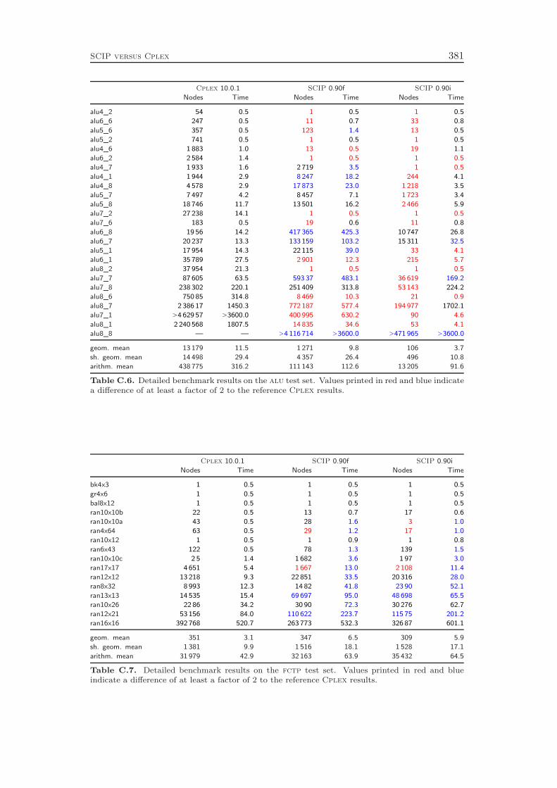
SCIP versus Cplex 381
Cplex 10.0.1 SCIP 0.90f SCIP 0.90i
Nodes Time Nodes Time Nodes Time
alu4_2 54 0.5 1 0.5 1 0.5
alu6_6 247 0.5 11 0.7 33 0.8
alu5_6 357 0.5 123 1.4 13 0.5
alu5_2 741 0.5 1 0.5 1 0.5
alu4_6 1 883 1.0 13 0.5 19 1.1
alu6_2 2 584 1.4 1 0.5 1 0.5
alu4_7 1 933 1.6 2 719 3.5 1 0.5
alu4_1 1 944 2.9 8 247 18.2 244 4.1
alu4_8 4 578 2.9 17 873 23.0 1 218 3.5
alu5_7 7 497 4.2 8 457 7.1 1 723 3.4
alu5_8 18 746 11.7 13 501 16.2 2 466 5.9
alu7_2 27 238 14.1 1 0.5 1 0.5
alu7_6 183 0.5 19 0.6 11 0.8
alu6_8 19 56 14.2 417 365 425.3 10 747 26.8
alu6_7 20 237 13.3 133 159 103.2 15 311 32.5
alu5_1 17 954 14.3 22 115 39.0 33 4.1
alu6_1 35 789 27.5 2 901 12.3 215 5.7
alu8_2 37 954 21.3 1 0.5 1 0.5
alu7_7 87 605 63.5 593 37 483.1 36 619 169.2
alu7_8 238 302 220.1 251 409 313.8 53 143 224.2
alu8_6 750 85 314.8 8 469 10.3 21 0.9
alu8_7 2 386 17 1450.3 772 187 577.4 194 977 1702.1
alu7_1 >4 629 57 >3600.0 400 995 630.2 90 4.6
alu8_1 2 240 568 1807.5 14 835 34.6 53 4.1
alu8_8 — — >4 116 714 >3600.0 >471 965 >3600.0
geom. mean 13 179 11.5 1 271 9.8 106 3.7
sh. geom. mean 14 498 29.4 4 357 26.4 496 10.8
arithm. mean 438 775 316.2 111 143 112.6 13 205 91.6
Table C.6. Detailed benchmark results on the alu test set. Values printed in red and blue indicatea difference of at least a factor of 2 to the reference Cplex results.
Cplex 10.0.1 SCIP 0.90f SCIP 0.90i
Nodes Time Nodes Time Nodes Time
bk4x3 1 0.5 1 0.5 1 0.5
gr4x6 1 0.5 1 0.5 1 0.5
bal8x12 1 0.5 1 0.5 1 0.5
ran10x10b 22 0.5 13 0.7 17 0.6
ran10x10a 43 0.5 28 1.6 3 1.0
ran4x64 63 0.5 29 1.2 17 1.0
ran10x12 1 0.5 1 0.9 1 0.8
ran6x43 122 0.5 78 1.3 139 1.5
ran10x10c 2 5 1.4 1 682 3.6 1 97 3.0
ran17x17 4 651 5.4 1 667 13.0 2 108 11.4
ran12x12 13 218 9.3 22 851 33.5 20 316 28.0
ran8x32 8 993 12.3 14 82 41.8 23 90 52.1
ran13x13 14 535 15.4 69 697 95.0 48 698 65.5
ran10x26 22 86 34.2 30 90 72.3 30 276 62.7
ran12x21 53 156 84.0 110 622 223.7 115 75 201.2
ran16x16 392 768 520.7 263 773 532.3 326 87 601.1
geom. mean 351 3.1 347 6.5 309 5.9
sh. geom. mean 1 381 9.9 1 516 18.1 1 528 17.1
arithm. mean 31 979 42.9 32 163 63.9 35 432 64.5
Table C.7. Detailed benchmark results on the fctp test set. Values printed in red and blueindicate a difference of at least a factor of 2 to the reference Cplex results.
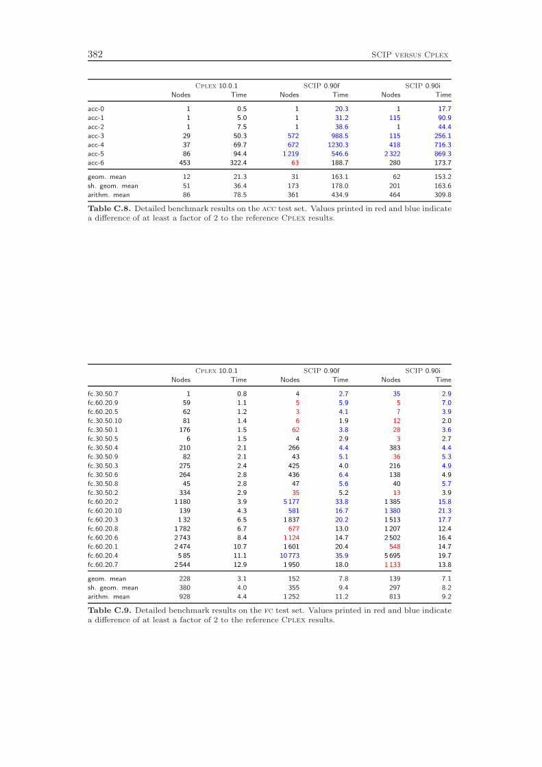
382 SCIP versus Cplex
Cplex 10.0.1 SCIP 0.90f SCIP 0.90i
Nodes Time Nodes Time Nodes Time
acc-0 1 0.5 1 20.3 1 17.7
acc-1 1 5.0 1 31.2 115 90.9
acc-2 1 7.5 1 38.6 1 44.4
acc-3 29 50.3 572 988.5 115 256.1
acc-4 37 69.7 672 1230.3 418 716.3
acc-5 86 94.4 1 219 546.6 2 322 869.3
acc-6 453 322.4 63 188.7 280 173.7
geom. mean 12 21.3 31 163.1 62 153.2
sh. geom. mean 51 36.4 173 178.0 201 163.6
arithm. mean 86 78.5 361 434.9 464 309.8
Table C.8. Detailed benchmark results on the acc test set. Values printed in red and blue indicatea difference of at least a factor of 2 to the reference Cplex results.
Cplex 10.0.1 SCIP 0.90f SCIP 0.90i
Nodes Time Nodes Time Nodes Time
fc.30.50.7 1 0.8 4 2.7 35 2.9
fc.60.20.9 59 1.1 5 5.9 5 7.0
fc.60.20.5 62 1.2 3 4.1 7 3.9
fc.30.50.10 81 1.4 6 1.9 12 2.0
fc.30.50.1 176 1.5 62 3.8 28 3.6
fc.30.50.5 6 1.5 4 2.9 3 2.7
fc.30.50.4 210 2.1 266 4.4 383 4.4
fc.30.50.9 82 2.1 43 5.1 36 5.3
fc.30.50.3 275 2.4 425 4.0 216 4.9
fc.30.50.6 264 2.8 436 6.4 138 4.9
fc.30.50.8 45 2.8 47 5.6 40 5.7
fc.30.50.2 334 2.9 35 5.2 13 3.9
fc.60.20.2 1 180 3.9 5 177 33.8 1 385 15.8
fc.60.20.10 139 4.3 581 16.7 1 380 21.3
fc.60.20.3 1 32 6.5 1 837 20.2 1 513 17.7
fc.60.20.8 1 782 6.7 677 13.0 1 207 12.4
fc.60.20.6 2 743 8.4 1 124 14.7 2 502 16.4
fc.60.20.1 2 474 10.7 1 601 20.4 548 14.7
fc.60.20.4 5 85 11.1 10 773 35.9 5 695 19.7
fc.60.20.7 2 544 12.9 1 950 18.0 1 133 13.8
geom. mean 228 3.1 152 7.8 139 7.1
sh. geom. mean 380 4.0 355 9.4 297 8.2
arithm. mean 928 4.4 1 252 11.2 813 9.2
Table C.9. Detailed benchmark results on the fc test set. Values printed in red and blue indicatea difference of at least a factor of 2 to the reference Cplex results.
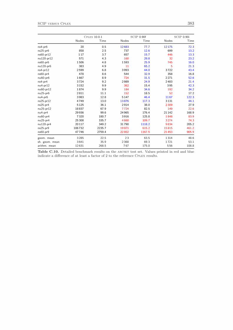
SCIP versus Cplex 383
Cplex 10.0.1 SCIP 0.90f SCIP 0.90i
Nodes Time Nodes Time Nodes Time
ns4-pr6 20 0.5 12 683 77.7 12 175 72.3
ns25-pr6 858 2.5 737 12.6 699 13.2
ns60-pr12 1 17 3.7 657 15.7 446 13.3
nu120-pr12 571 4.3 160 29.8 32 23.2
ns60-pr6 1 506 4.8 1 593 25.9 745 16.0
nu120-pr6 383 4.9 11 65.2 5 21.3
ns4-pr12 2 599 6.8 3 993 44.0 3 722 43.4
ns60-pr4 478 8.6 544 32.9 358 16.8
nu60-pr6 1 667 8.9 724 31.5 2 271 52.6
ns4-pr4 3 724 9.2 2 989 24.9 2 483 21.4
nu4-pr12 3 152 9.9 362 15.4 3 95 42.3
nu60-pr12 1 874 9.9 184 34.6 192 34.2
nu25-pr6 2 811 11.1 152 18.5 52 17.2
nu4-pr6 3 983 12.8 5 147 46.4 11 67 122.3
ns25-pr12 4 749 13.0 13 876 117.3 3 131 44.1
ns25-pr4 5 125 36.1 2 914 38.0 2 309 27.9
nu25-pr12 18 837 67.9 7 724 82.5 149 22.6
nu4-pr4 29 936 99.6 24 965 176.4 21 142 168.9
nu60-pr4 7 320 180.7 3 916 125.8 1 848 83.9
nu25-pr4 25 308 335.7 4 660 109.7 3 274 74.3
nu120-pr4 20 117 349.2 31 790 1118.2 9 834 205.2
ns25-pr9 106 732 2235.7 19 971 615.2 15 815 461.2
ns60-pr9 47 746 2759.4 22 802 1167.5 21 453 905.9
geom. mean 3 285 22.5 2 3 63.5 1 314 48.6
sh. geom. mean 3 641 35.9 2 368 69.3 1 721 53.1
arithm. mean 12 631 268.5 7 67 175.0 5 56 108.8
Table C.10. Detailed benchmark results on the arcset test set. Values printed in red and blueindicate a difference of at least a factor of 2 to the reference Cplex results.
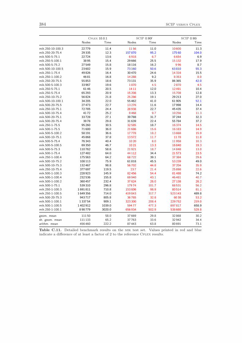
384 SCIP versus Cplex
Cplex 10.0.1 SCIP 0.90f SCIP 0.90i
Nodes Time Nodes Time Nodes Time
mik.250-10-100.3 22 779 11.4 11 56 11.0 10 600 11.3
mik.250-20-75.4 29 335 12.3 157 870 95.2 175 60 104.0
mik.500-5-75.1 22 724 13.6 6 918 6.7 6 654 6.9
mik.250-5-100.1 38 95 15.4 29 666 25.5 15 132 17.9
mik.500-5-75.2 27 549 15.8 18 116 16.2 9 96 8.7
mik.500-10-100.5 23 602 15.9 73 160 50.6 63 810 55.3
mik.250-1-75.4 49 826 16.4 30 470 24.6 14 316 15.5
mik.250-1-100.2 46 81 16.8 14 288 9.2 8 353 8.0
mik.250-20-75.5 55 853 18.6 73 131 35.9 86 365 42.0
mik.500-5-100.3 33 967 19.6 1 870 4.5 2 870 4.5
mik.250-5-75.1 61 46 20.5 14 11 12.0 12 491 10.4
mik.250-5-75.4 65 293 20.9 15 208 13.3 15 708 12.8
mik.250-10-75.2 56 824 21.8 25 286 19.1 29 213 27.0
mik.500-10-100.1 34 205 22.0 55 462 41.0 61 905 52.1
mik.500-20-75.5 27 473 22.7 13 276 11.6 17 998 14.4
mik.250-10-75.1 72 785 24.4 28 938 22.7 45 435 37.4
mik.500-10-75.4 41 72 25.2 9 468 9.7 10 256 11.3
mik.500-20-75.1 33 728 27.1 39 788 31.7 37 244 32.3
mik.500-20-75.4 39 78 29.8 31 639 22.4 55 784 37.2
mik.250-1-75.5 95 260 30.5 32 585 18.7 16 374 14.5
mik.500-1-75.5 71 600 36.0 21 686 15.6 16 183 14.9
mik.500-5-100.2 58 191 36.6 17 778 18.2 13 888 15.9
mik.500-10-75.1 45 868 37.8 13 572 11.7 11 78 11.8
mik.500-5-75.4 76 343 40.4 10 20 8.0 11 958 10.3
mik.500-5-100.5 69 350 46.7 10 21 13.3 16 840 19.3
mik.500-5-75.3 110 762 58.6 21 921 18.7 14 848 13.0
mik.500-1-75.4 127 482 64.0 44 112 34.4 21 573 23.5
mik.250-1-100.4 175 563 64.2 68 722 39.1 37 384 29.6
mik.500-10-75.2 108 113 75.9 61 818 45.5 53 239 49.0
mik.500-10-75.3 132 467 98.8 56 702 44.8 37 204 35.9
mik.250-10-75.4 377 697 119.5 23 7 21.4 25 898 22.6
mik.500-1-100.3 228 923 145.9 82 456 54.4 81 488 74.2
mik.500-1-100.4 232 536 155.8 69 940 43.1 46 481 40.7
mik.500-1-100.2 360 457 232.4 37 624 26.0 27 138 26.2
mik.500-1-75.1 539 310 296.8 179 74 101.7 68 531 56.2
mik.250-1-100.3 1 691 811 710.8 153 606 98.9 80 514 81.1
mik.250-1-100.5 1 649 356 714.0 419 843 317.7 523 143 489.8
mik.500-20-75.3 943 717 805.8 36 765 32.8 60 38 53.2
mik.500-1-100.1 1 337 54 909.1 323 300 208.4 229 752 219.0
mik.500-1-100.5 1 402 912 1039.0 594 77 477.3 697 817 658.9
mik.250-1-100.1 8 98 779 3020.0 656 934 502.9 538 680 529.8
geom. mean 111 50 58.0 37 669 29.8 32 868 30.2
sh. geom. mean 111 133 65.2 37 763 33.6 32 942 34.4
arithm. mean 456 460 222.2 87 443 63.8 80 691 73.1
Table C.11. Detailed benchmark results on the mik test set. Values printed in red and blueindicate a difference of at least a factor of 2 to the reference Cplex results.
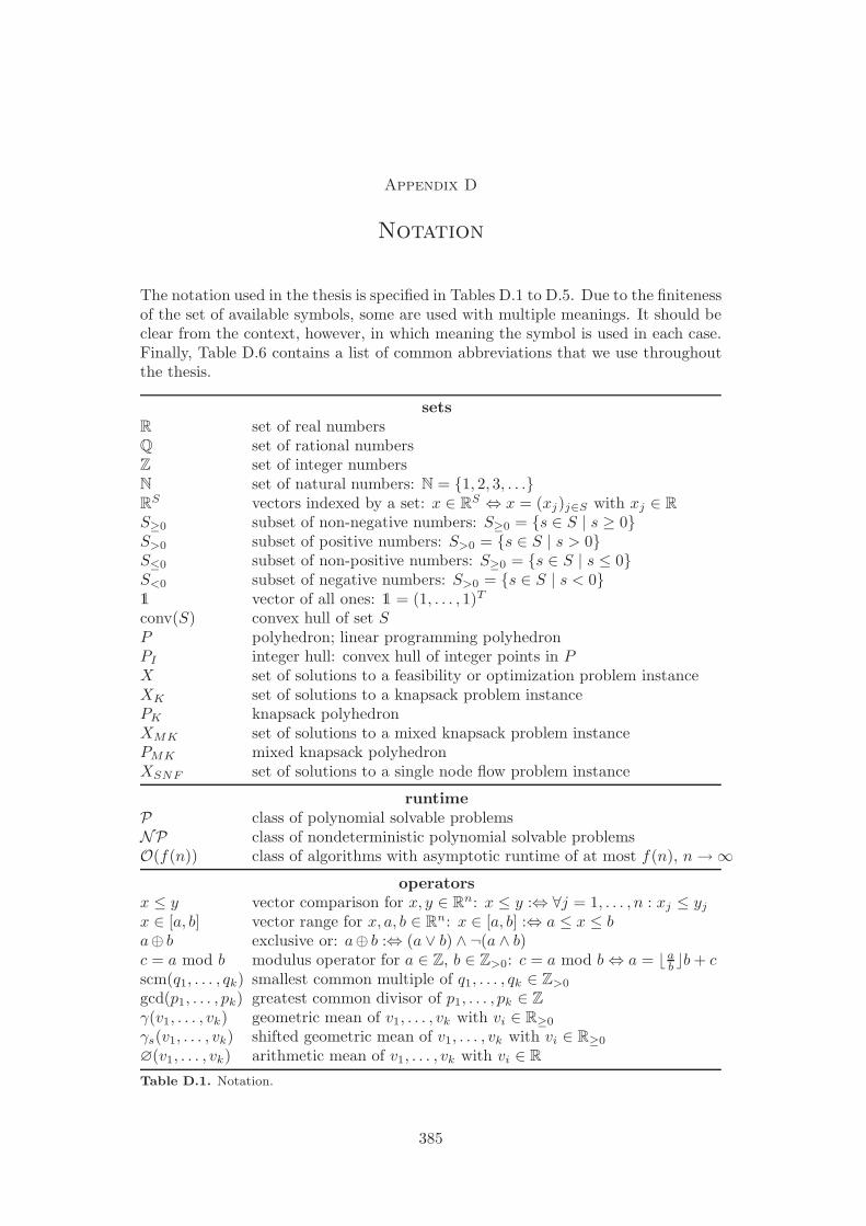
Appendix D
Notation
The notation used in the thesis is specified in Tables D.1 to D.5. Due to the finitenessof the set of available symbols, some are used with multiple meanings. It should beclear from the context, however, in which meaning the symbol is used in each case.Finally, Table D.6 contains a list of common abbreviations that we use throughoutthe thesis.
setsR set of real numbersQ set of rational numbersZ set of integer numbersN set of natural numbers: N = {1, 2, 3, . . .}RS vectors indexed by a set: x ∈ RS ⇔ x = (xj)j∈S with xj ∈ RS≥0 subset of non-negative numbers: S≥0 = {s ∈ S | s ≥ 0}S>0 subset of positive numbers: S>0 = {s ∈ S | s > 0}S≤0 subset of non-positive numbers: S≥0 = {s ∈ S | s ≤ 0}S<0 subset of negative numbers: S>0 = {s ∈ S | s < 0}1 vector of all ones: 1 = (1, . . . , 1)T
conv(S) convex hull of set SP polyhedron; linear programming polyhedronPI integer hull: convex hull of integer points in PX set of solutions to a feasibility or optimization problem instanceXK set of solutions to a knapsack problem instancePK knapsack polyhedronXMK set of solutions to a mixed knapsack problem instancePMK mixed knapsack polyhedronXSNF set of solutions to a single node flow problem instance
runtimeP class of polynomial solvable problemsNP class of nondeterministic polynomial solvable problemsO(f(n)) class of algorithms with asymptotic runtime of at most f(n), n→∞
operatorsx ≤ y vector comparison for x, y ∈ Rn: x ≤ y :⇔ ∀j = 1, . . . , n : xj ≤ yj
x ∈ [a, b] vector range for x, a, b ∈ Rn: x ∈ [a, b] :⇔ a ≤ x ≤ ba⊕ b exclusive or: a⊕ b :⇔ (a ∨ b) ∧ ¬(a ∧ b)c = a mod b modulus operator for a ∈ Z, b ∈ Z>0: c = a mod b⇔ a = ⌊a
b⌋b+ c
scm(q1, . . . , qk) smallest common multiple of q1, . . . , qk ∈ Z>0
gcd(p1, . . . , pk) greatest common divisor of p1, . . . , pk ∈ Zγ(v1, . . . , vk) geometric mean of v1, . . . , vk with vi ∈ R≥0
γs(v1, . . . , vk) shifted geometric mean of v1, . . . , vk with vi ∈ R≥0
∅(v1, . . . , vk) arithmetic mean of v1, . . . , vk with vi ∈ R
Table D.1. Notation.
385
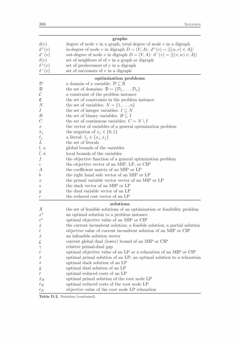
386 Notation
graphsd(v) degree of node v in a graph, total degree of node v in a digraphd+(v) in-degree of node v in digraph D = (V,A): d+(v) = |{(u, v) ∈ A}|d−(v) out-degree of node v in digraph D = (V,A): d−(v) = |{(v,w) ∈ A}|δ(v) set of neighbors of of v in a graph or digraphδ+(v) set of predecessors of v in a digraphδ−(v) set of successors of v in a digraph
optimization problemsD a domain of a variable: D ⊆ RD the set of domains: D = {D1, . . . ,Dn}C a constraint of the problem instanceC the set of constraints in the problem instanceN the set of variables: N = {1, . . . , n}I the set of integer variables: I ⊆ NB the set of binary variables: B ⊆ IC the set of continuous variables: C = N \ Ix the vector of variables of a general optimization problemxj the negation of xj ∈ {0, 1}ℓj a literal: ℓj ∈ {xj , xj}L the set of literalsl, u global bounds of the variables
l, u local bounds of the variablesf the objective function of a general optimization problemc the objective vector of an MIP, LP, or CIPA the coefficient matrix of an MIP or LPb the right hand side vector of an MIP or LPx the primal variable vector vector of an MIP or LPs the slack vector of an MIP or LPy the dual variable vector of an LPr the reduced cost vector of an LP
solutionsX the set of feasible solutions of an optimization or feasibility problemx⋆ an optimal solution to a problem instancec⋆ optimal objective value of an MIP or CIPx the current incumbent solution; a feasible solution; a partial solutionc objective value of current incumbent solution of an MIP or CIPx an infeasible solution vectorc current global dual (lower) bound of an MIP or CIPγ relative primal-dual gapc optimal objective value of an LP or a relaxation of an MIP or CIPx optimal primal solution of an LP; an optimal solution to a relaxations optimal slack solution of an LPy optimal dual solution of an LPr optimal reduced costs of an LPxR optimal primal solution of the root node LPrR optimal reduced costs of the root node LPcR objective value of the root node LP relaxation
Table D.2. Notation (continued).

Notation 387
numerics
δ primal feasibility tolerance of SCIP (default is δ = 10−6)δ dual feasibility (LP optimality) tolerance of SCIP (default is δ = 10−9)ǫ zero tolerance of SCIP (default is ǫ = 10−9)
x.= y equality within feasibility tolerance: x
.= y ⇔ |x−y|
max{|x|,|y|,1} ≤ δ
constraintsalldiff all-different constraint: all variables must take a different valueelement element constraint: selects a single element of a listnosubtour no-subtour constraint: forbids subtours in a TSP instancesppc set packing, partitioning, or covering constraint
β, β left and right hand sides of a linear constraint β ≤ aTx ≤ βa coefficient vector of a linear constraintα current activity of a linear constraint: α(x) = aTxα, α activity bounds of a linear constraint w.r.t. the variables’ boundsF0 current number of variables of a sppc constraint that are fixed to 0F1 current number of variables of a sppc constraint that are fixed to 1
branch-and-boundR global problem, root of the search treeQ current subproblemS sibling of the current subproblemp(Q) parent node of subproblem QL leaf subproblem in the search treeS list of siblings of the current subproblemC list of children of the current subproblemL list of open subproblems; leaves in the search treeA active path from the root node to the current subproblemQrelax relaxation of subproblem QQLP LP relaxation of subproblem Q
simplex algorithmB set of basic variablesN set of non-basic variablesa row in the simplex tableau A = A−1
B A
data structuresQ clique: set of binary variables of which at most one can set to 1Q clique table
Table D.3. Notation (continued).
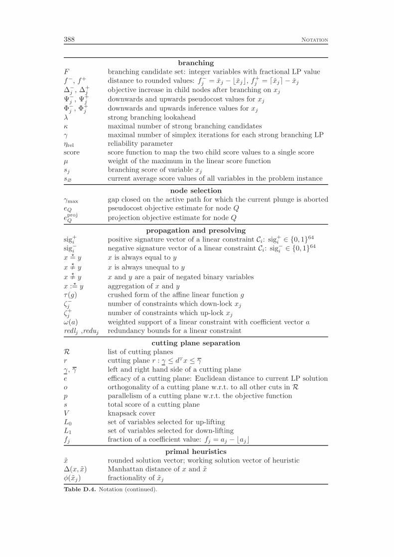
388 Notation
branchingF branching candidate set: integer variables with fractional LP valuef−, f+ distance to rounded values: f−j = xj − ⌊xj⌋, f
+j = ⌈xj⌉ − xj
∆−j , ∆+j objective increase in child nodes after branching on xj
Ψ−j , Ψ+j downwards and upwards pseudocost values for xj
Φ−j , Φ+j downwards and upwards inference values for xj
λ strong branching lookaheadκ maximal number of strong branching candidatesγ maximal number of simplex iterations for each strong branching LPηrel reliability parameterscore score function to map the two child score values to a single scoreµ weight of the maximum in the linear score functionsj branching score of variable xj
s∅ current average score values of all variables in the problem instance
node selectionγmax gap closed on the active path for which the current plunge is abortedeQ pseudocost objective estimate for node Q
eprojQ projection objective estimate for node Q
propagation and presolvingsig+
i positive signature vector of a linear constraint Ci: sig+i ∈ {0, 1}
64
sig−i negative signature vector of a linear constraint Ci: sig−i ∈ {0, 1}64
x ⋆= y x is always equal to y
x Y⋆= y x is always unequal to y
x Y⋆= y x and y are a pair of negated binary variables
x : ⋆= y aggregation of x and yτ(g) crushed form of the affine linear function gζ−j number of constraints which down-lock xj
ζ+j number of constraints which up-lock xj
ω(a) weighted support of a linear constraint with coefficient vector aredlj ,reduj redundancy bounds for a linear constraint
cutting plane separationR list of cutting planesr cutting plane r : γ ≤ dTx ≤ γγ, γ left and right hand side of a cutting planee efficacy of a cutting plane: Euclidean distance to current LP solutiono orthogonality of a cutting plane w.r.t. to all other cuts in Rp parallelism of a cutting plane w.r.t. the objective functions total score of a cutting planeV knapsack coverL0 set of variables selected for up-liftingL1 set of variables selected for down-liftingfj fraction of a coefficient value: fj = aj − ⌊aj⌋
primal heuristicsx rounded solution vector; working solution vector of heuristic∆(x, x) Manhattan distance of x and xφ(xj) fractionality of xj
Table D.4. Notation (continued).
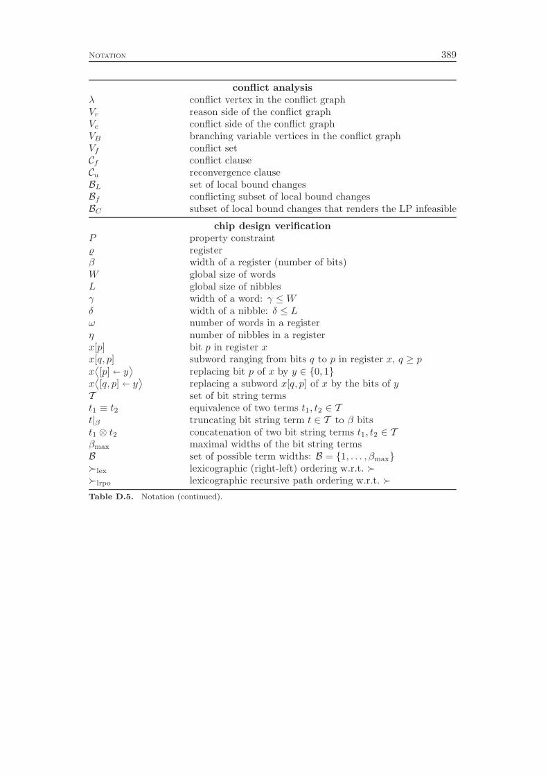
Notation 389
conflict analysisλ conflict vertex in the conflict graphVr reason side of the conflict graphVc conflict side of the conflict graphVB branching variable vertices in the conflict graphVf conflict setCf conflict clauseCu reconvergence clauseBL set of local bound changesBf conflicting subset of local bound changesBC subset of local bound changes that renders the LP infeasible
chip design verificationP property constraint registerβ width of a register (number of bits)W global size of wordsL global size of nibblesγ width of a word: γ ≤ Wδ width of a nibble: δ ≤ Lω number of words in a registerη number of nibbles in a registerx[p] bit p in register xx[q, p] subword ranging from bits q to p in register x, q ≥ px⟨[p] � y
⟩replacing bit p of x by y ∈ {0, 1}
x⟨[q, p] � y
⟩replacing a subword x[q, p] of x by the bits of y
T set of bit string termst1 ≡ t2 equivalence of two terms t1, t2 ∈ Tt|β truncating bit string term t ∈ T to β bitst1 ⊗ t2 concatenation of two bit string terms t1, t2 ∈ Tβmax maximal widths of the bit string termsB set of possible term widths: B = {1, . . . , βmax}≻lex lexicographic (right-left) ordering w.r.t. ≻≻lrpo lexicographic recursive path ordering w.r.t. ≻
Table D.5. Notation (continued).
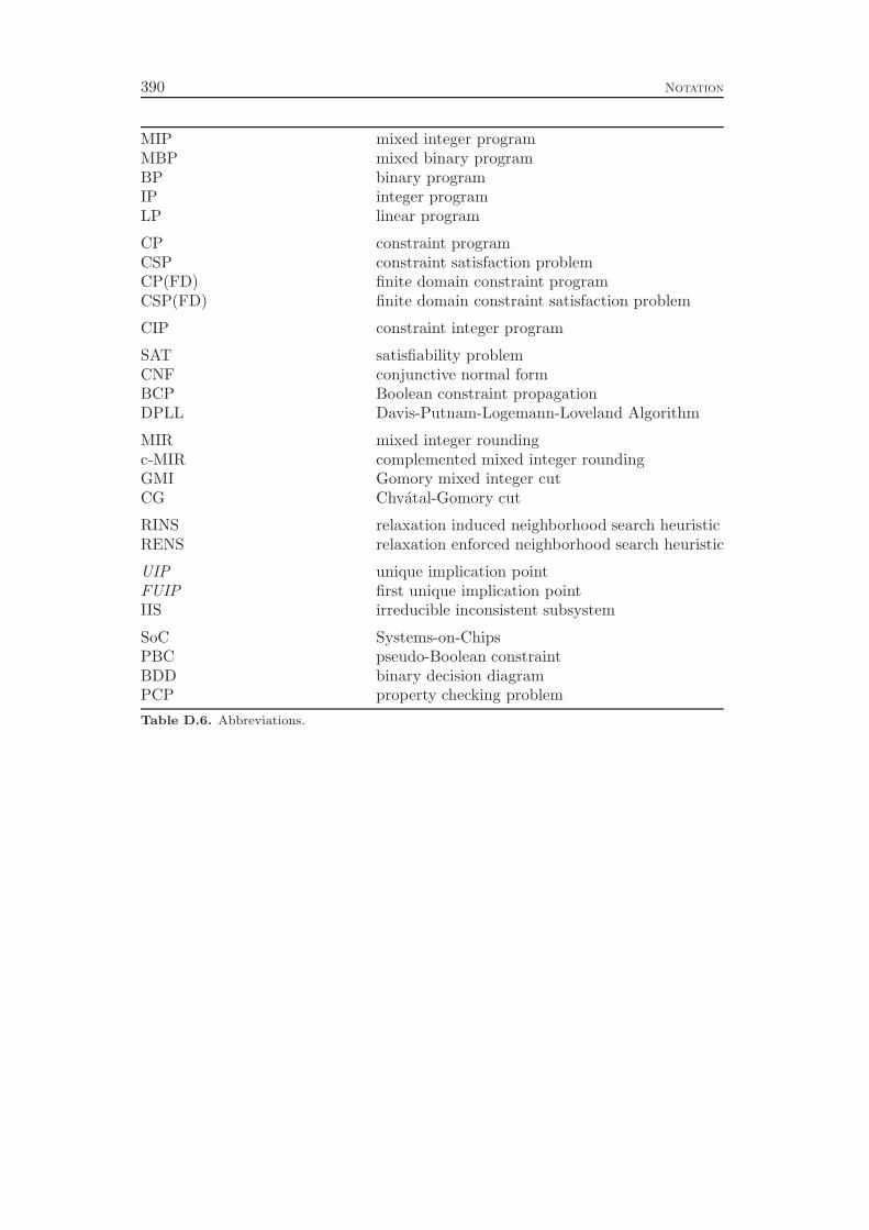
390 Notation
MIP mixed integer programMBP mixed binary programBP binary programIP integer programLP linear program
CP constraint programCSP constraint satisfaction problemCP(FD) finite domain constraint programCSP(FD) finite domain constraint satisfaction problem
CIP constraint integer program
SAT satisfiability problemCNF conjunctive normal formBCP Boolean constraint propagationDPLL Davis-Putnam-Logemann-Loveland Algorithm
MIR mixed integer roundingc-MIR complemented mixed integer roundingGMI Gomory mixed integer cutCG Chvátal-Gomory cut
RINS relaxation induced neighborhood search heuristicRENS relaxation enforced neighborhood search heuristic
UIP unique implication pointFUIP first unique implication pointIIS irreducible inconsistent subsystem
SoC Systems-on-ChipsPBC pseudo-Boolean constraintBDD binary decision diagramPCP property checking problem
Table D.6. Abbreviations.
List of Algorithms
2.1 Branch-and-bound . . . . . . . . . . . . . . . . . . . . . . . . . . . . 163.1 Node Switching . . . . . . . . . . . . . . . . . . . . . . . . . . . . . . 463.2 Cutting Plane Selection . . . . . . . . . . . . . . . . . . . . . . . . . 495.1 Generic variable selection . . . . . . . . . . . . . . . . . . . . . . . . 615.2 Reliability branching . . . . . . . . . . . . . . . . . . . . . . . . . . . 657.1 Domain Propagation for Linear Constraints . . . . . . . . . . . . . . 887.2 Event Handler for Linear Constraints . . . . . . . . . . . . . . . . . . 897.3 Domain Propagation for Knapsack Constraints . . . . . . . . . . . . 907.4 Event Handler for Knapsack Constraints . . . . . . . . . . . . . . . . 917.5 Domain Propagation for Set Partitioning/Packing Constraints . . . . 927.6 Event Handler for Set Partitioning/Packing Constraints . . . . . . . 927.7 Domain Propagation for Set Covering Constraints . . . . . . . . . . 957.8 Event Handler for Set Covering Constraints . . . . . . . . . . . . . . 957.9 Domain Propagation for Variable Bound Constraints . . . . . . . . . 977.10 Event Handler for Variable Bound Constraints . . . . . . . . . . . . 977.11 Root Reduced Cost Strengthening . . . . . . . . . . . . . . . . . . . 988.1 Separation of Lifted Knapsack Cover Cuts . . . . . . . . . . . . . . . 1038.2 Separation of Complemented MIR Cuts . . . . . . . . . . . . . . . . 1059.1 Generic Diving Heuristic . . . . . . . . . . . . . . . . . . . . . . . . . 12110.1 Presolving for Linear Constraints . . . . . . . . . . . . . . . . . . . . 13410.2 Normalization of Linear Constraints . . . . . . . . . . . . . . . . . . 13510.3 Presolving of Linear Equations . . . . . . . . . . . . . . . . . . . . . 13710.4 Dual Aggregation for Linear Constraints . . . . . . . . . . . . . . . . 13910.5 Pairwise Presolving of Linear Constraints . . . . . . . . . . . . . . . 14110.6 Dual Bound Reduction for Linear Constraints . . . . . . . . . . . . . 14310.7 Upgrading of Linear Constraints . . . . . . . . . . . . . . . . . . . . 14510.8 Presolving for Knapsack Constraints . . . . . . . . . . . . . . . . . . 14710.9 Presolving for Set Partitioning, Packing, and Covering Constraints . 15210.10Presolving for Variable Bound Constraints . . . . . . . . . . . . . . . 15310.11Integer to Binary Conversion . . . . . . . . . . . . . . . . . . . . . . 15410.12Probing . . . . . . . . . . . . . . . . . . . . . . . . . . . . . . . . . . 15610.13Implication Graph Analysis . . . . . . . . . . . . . . . . . . . . . . . 15810.14Dual Fixing . . . . . . . . . . . . . . . . . . . . . . . . . . . . . . . . 15911.1 Infeasible LP Analysis . . . . . . . . . . . . . . . . . . . . . . . . . . 17511.2 Bound Exceeding LP Analysis . . . . . . . . . . . . . . . . . . . . . . 17714.1 Bit and Word Partitioning Domain Propagation . . . . . . . . . . . 19814.2 Bit and Word Partitioning Presolving . . . . . . . . . . . . . . . . . 20214.3 Addition Domain Propagation . . . . . . . . . . . . . . . . . . . . . . 20714.4 Addition Presolving . . . . . . . . . . . . . . . . . . . . . . . . . . . 20814.5 Addition Presolving – Bit Aggregation . . . . . . . . . . . . . . . . . 20914.6 Addition Presolving – Implications . . . . . . . . . . . . . . . . . . . 21014.7 Multiplication Domain Propagation – LP Propagation . . . . . . . . 21514.8 Multiplication Domain Propagation – Binary Propagation . . . . . . 21814.9 Multiplication Domain Propagation – Term Normalization . . . . . . 221
391
392 List of Algorithms
14.10Multiplication Domain Propagation – Symbolic Propagation . . . . . 22414.11Multiplication Domain Propagation – Variable-Term Equation . . . 22514.12Multiplication Presolving . . . . . . . . . . . . . . . . . . . . . . . . 22614.13Bitwise And Domain Propagation . . . . . . . . . . . . . . . . . . . . 23014.14Bitwise And Presolving . . . . . . . . . . . . . . . . . . . . . . . . . 23014.15Bitwise Xor Domain Propagation . . . . . . . . . . . . . . . . . . . . 23314.16Bitwise Xor Presolving . . . . . . . . . . . . . . . . . . . . . . . . . . 23414.17Unary And Domain Propagation . . . . . . . . . . . . . . . . . . . . 23514.18Unary And Presolving . . . . . . . . . . . . . . . . . . . . . . . . . . 23614.19Unary Xor Domain Propagation . . . . . . . . . . . . . . . . . . . . 23914.20Unary Xor Presolving . . . . . . . . . . . . . . . . . . . . . . . . . . 24014.21Equality Domain Propagation . . . . . . . . . . . . . . . . . . . . . . 24314.22Equality Presolving . . . . . . . . . . . . . . . . . . . . . . . . . . . . 24514.23Less-Than Domain Propagation . . . . . . . . . . . . . . . . . . . . . 24914.24Less-Than Presolving . . . . . . . . . . . . . . . . . . . . . . . . . . . 25014.25If-Then-Else Domain Propagation . . . . . . . . . . . . . . . . . . . . 25414.26If-Then-Else Presolving . . . . . . . . . . . . . . . . . . . . . . . . . 25514.27Shift Left Domain Propagation . . . . . . . . . . . . . . . . . . . . . 26114.28Shift Left Presolving . . . . . . . . . . . . . . . . . . . . . . . . . . . 26314.29Slice Domain Propagation . . . . . . . . . . . . . . . . . . . . . . . . 26614.30Slice Presolving . . . . . . . . . . . . . . . . . . . . . . . . . . . . . . 26814.31Multiplex Read Domain Propagation . . . . . . . . . . . . . . . . . . 27114.32Multiplex Read Presolving . . . . . . . . . . . . . . . . . . . . . . . . 27214.33Multiplex Write Domain Propagation . . . . . . . . . . . . . . . . . 27514.34Multiplex Write Presolving . . . . . . . . . . . . . . . . . . . . . . . 27615.1 Term Algebra Preprocessing – Term Normalization . . . . . . . . . . 28315.2 Term Algebra Preprocessing . . . . . . . . . . . . . . . . . . . . . . . 28615.3 Term Algebra Preprocessing – Self-Reference Simplification . . . . . 28615.4 Term Algebra Preprocessing – Zero Resultant Simplification . . . . . 28715.5 Term Algebra Preprocessing – Deductions on Resultant Bits . . . . . 28815.6 Term Algebra Preprocessing – Operand Substitution . . . . . . . . . 28915.7 Irrelevance Detection . . . . . . . . . . . . . . . . . . . . . . . . . . . 292

Bibliography
[1] T. Achterberg, Conflict analysis in mixed integer programming, Discrete Optimiza-tion 4, no. 1 (2007), pp. 4–20. Special issue: Mixed Integer Programming.
[2] T. Achterberg and T. Berthold, Improving the feasibility pump, Discrete Opti-mization 4, no. 1 (2007), pp. 77–86. Special issue: Mixed Integer Programming.
[3] T. Achterberg, M. Grötschel, and T. Koch, Teaching MIP modeling and solv-ing, ORMS Today 33, no. 6 (2006), pp. 14–15.
[4] T. Achterberg, T. Koch, and A. Martin, The mixed integer programming library:Miplib 2003. Zuse Institute Berlin, http://miplib.zib.de.
[5] T. Achterberg, T. Koch, and A. Martin, Branching rules revisited, OperationsResearch Letters 33 (2005), pp. 42–54.
[6] T. Achterberg, T. Koch, and A. Martin, MIPLIB 2003, Operations ResearchLetters 34, no. 4 (2006), pp. 1–12.
[7] A. Aiba, K. Sakai, Y. Sato, D. J. Hawley, and R. Hasegawa, Constraint logicprogramming language CAL, in FGCS-88: Proceedings of the International Confer-ence on Fifth Generation Computer Systems, Tokyo, 1988, pp. 263–276.
[8] S. B. Akers, Binary decision diagrams, IEEE Transactions on Computers C-27,no. 6 (1978), pp. 509–516.
[9] R. B. J. T. Allenby, Rings, Fields and Groups, Arnold, 1991.
[10] E. Althaus, A. Bockmayr, M. Elf, M. Jünger, T. Kasper, and K. Mehlhorn,SCIL – symbolic constraints in integer linear programming, Tech. Report ALCOMFT-TR-02-133, MPI Saarbrücken, May 2002.
[11] E. Amaldi, M. E. Pfetsch, and L. E. Trotter, Jr., On the maximum feasiblesubsystem problem, IISs, and IIS-hypergraphs, Mathematical Programming 95, no. 3(2003), pp. 533–554.
[12] C. Anders, Das Chordalisierungspolytop und die Berechnung der Baumweite einesGraphen, master’s thesis, Technische Universität Berlin, 2006.
[13] G. Andreello, A. Caprara, and M. Fischetti, Embedding cuts in a branch&cutframework: a computational study with {0, 1
2}-cuts, INFORMS Journal on Comput-
ing (2007).
[14] D. Applegate, R. E. Bixby, V. Chvátal, and W. Cook, Finding cuts in theTSP, Tech. Report 95-05, DIMACS, March 1995.
[15] D. Applegate, R. E. Bixby, V. Chvátal, and W. Cook, On the solution oftraveling salesman problems, Documenta Mathematica ICM III (1998), pp. 645–656.
[16] D. Applegate, R. E. Bixby, V. Chvátal, and W. Cook, TSP cuts which do notconform to the template paradigm, in Computational Combinatorial Optimization,M. Jünger and D. Naddef, eds., Springer, Heidelberg, Germany, 2001, pp. 261–304.
[17] K. R. Apt, Principles of Constraint Programming, Cambridge University Press,2003.
[18] M. Armbruster, Branch-and-Cut for a Semidefinite Relaxation of the MinimumBisection Problem, PhD thesis, Technische Universität Chemnitz, 2007.
[19] M. Armbruster, M. Fügenschuh, C. Helmberg, and A. Martin, Experimentswith linear and semidefinite relaxations for solving the minimum graph bisection prob-lem, tech. report, Darmstadt University of Technology, November 2006.
393
394 Bibliography
[20] M. Armbruster, M. Fügenschuh, C. Helmberg, and A. Martin, On the bisec-tion cut polytope, preprint, Darmstadt University of Technology, November 2006.
[21] I. D. Aron, J. N. Hooker, and T. H. Yunes, SIMPL: A system for integratingoptimization techniques, in Integration of AI and OR Techniques in Constraint Pro-gramming for Combinatorial Optimization Problems, First International Conference,CPAIOR 2004, J.-C. Régin and M. Rueher, eds., Lecture Notes in Computer Science3011, Nice, France, April 2004, Springer, pp. 21–36.
[22] A. Atamtürk, Flow pack facets of the single node fixed-charge flow polytope, Oper-ations Research Letters 29 (2001), pp. 107–114.
[23] A. Atamtürk, On the facets of the mixed–integer knapsack polyhedron, MathematicalProgramming 98 (2003), pp. 145–175.
[24] A. Atamtürk, G. L. Nemhauser, and M. W. P. Savelsbergh, Conflict graphs ininteger programming, European Journal of Operations Research 121 (2000), pp. 40–55.
[25] A. Atamtürk and D. Rajan, On splittable and unsplittable capacitated networkdesign arc-set polyhedra, Mathematical Programming 92 (2002), pp. 315–333.
[26] A. Atamtürk and M. W. P. Savelsbergh, Integer-programming software systems,Annals of Operations Research 140, no. 1 (2005), pp. 67–124.
[27] G. Audemard, P. Bertoli, A. Cimatti, A. Kornilowicz, and R. Sebastiani,A SAT-based approach for solving formulas over boolean and linear mathematicalpropositions, in Proc. Conference on Automated Deduction (CADE), 2002, pp. 195–210.
[28] E. Balas, Facets of the knapsack polytope, Mathematical Programming 8 (1975),pp. 146–164.
[29] E. Balas, S. Ceria, and G. Cornuéjols, A lift-and-project cutting plane algorithmfor mixed 0-1 programs, Mathematical Programming 58 (1993), pp. 295–324.
[30] E. Balas, S. Ceria, and G. Cornuéjols, Mixed 0-1 programming by lift-and-project in a branch-and-cut framework, Management Science 42 (1996), pp. 1229–1246.
[31] E. Balas, S. Ceria, G. Cornuéjols, and N. Natraj, Gomory cuts revisited,Operations Research Letters 19 (1996), pp. 1–9.
[32] E. Balas, S. Ceria, M. Dawande, F. Margot, and G. Pataki, OCTANE: A newheuristic for pure 0-1 programs, Operations Research 49, no. 2 (2001), pp. 207–225.
[33] E. Balas and C. H. Martin, Pivot-and-complement: A heuristic for 0-1 program-ming, Management Science 26, no. 1 (1980), pp. 86–96.
[34] E. Balas, S. Schmieta, and C. Wallace, Pivot and shift - a mixed integer pro-gramming heuristic, Discrete Optimization 1, no. 1 (2004), pp. 3–12.
[35] E. Balas and E. Zemel, Facets of the knapsack polytope from minimal covers, SIAMJournal on Applied Mathematics 34 (1978), pp. 119–148.
[36] E. Balas and E. Zemel, Lifting and complementing yields all the facets of positivezero-one programming polytopes, in Proceedings of the International Conference onMathematical Programming, Rio de Janeiro, 1981, R. W. Cottle, M. I. Kelmanson,and B. Korte, eds., Elsevier Science Publishers, 1984, pp. 13–24.
[37] E. M. L. Beale, Branch and bound methods for mathematical programming systems,in Discrete Optimization II, P. L. Hammer, E. L. Johnson, and B. H. Korte, eds.,North Holland Publishing Co., 1979, pp. 201–219.
[38] E. M. L. Beale and J. A. Tomlin, Special facilities in a general mathemati-cal programming system for non-convex problems using ordered sets of variables, inOR 69: Proceedings of the Fifth International Conference on Operations Research,J. Lawrence, ed., London, 1970, Tavistock Publications, pp. 447–454.
Bibliography 395
[39] M. Bénichou, J. M. Gauthier, P. Girodet, G. Hentges, G. Ribière, andO. Vincent, Experiments in mixed-integer linear programming, Mathematical Pro-gramming 1 (1971), pp. 76–94.
[40] L. Bertacco, M. Fischetti, and A. Lodi, A feasibility pump heuristic for generalmixed-integer problems, Tech. Report OR/05/5, DEIS – Università di Bologna, Italy,May 2005.
[41] T. Berthold, Primal heuristics for mixed integer programs, master’s thesis, Tech-nische Universität Berlin, 2006.
[42] A. Biere, A. Cimatti, E. M. Clarke, M. Fujita, and Y. Zhu, Symbolic modelchecking using SAT procedures instead of BDDs, in Proceedings of the InternationalDesign Automation Conference (DAC-99), June 1999, pp. 317–320.
[43] A. Biere, E. M. Clarke, R. Raimi, and Y. Zhu, Verifying safety properties of aPower PC microprocessor using symbolic model checking without BDDs, in Computer-Aided Verification, Lecture Notes in Computer Science 1633, Springer, 1999, pp. 60–71.
[44] A. Biere and W. Kunz, SAT and ATPG: Boolean engines for formal hardwareverification, in ACM/IEEE Intl. Conf. on Computer-Aided Design (ICCAD), SanJose, November 2002.
[45] E. Bilgen, Personalkostenminimierung bei der Einsatzplanung von parallelen iden-tischen Bearbeitungszentren in der Motorradproduktion, master’s thesis, TechnischeUniversität Chemnitz, 2007.
[46] R. E. Bixby, M. Fenelon, Z. Gu, E. Rothberg, and R. Wunderling, MIP: The-ory and practice – closing the gap, in Systems Modelling and Optimization: Methods,Theory, and Applications, M. Powell and S. Scholtes, eds., Kluwer, 2000, pp. 19–49.
[47] P. Bjesse, T. Leonard, and A. Mokkedem, Finding bugs in an Alpha micropro-cessor using satisfiability solvers, in Computer-Aided Verification, Lecture Notes inComputer Science 2102, Springer, 2001, pp. 454–464.
[48] A. Bley, F. Kupzog, and A. Zymolka, Auslegung heterogener Kommunikation-snetze nach Performance und Wirtschaftlichkeit, in Proceedings of 11th KasselerSymposium Energie-Systemtechnik: Energie und Kommunikation, Kassel, Novem-ber 2006, pp. 84–97.
[49] A. Bockmayr and T. Kasper, Branch-and-infer: A unifying framework for integerand finite domain constraint programming, INFORMS Journal on Computing 10,no. 3 (1998), pp. 287–300.
[50] A. Bockmayr and N. Pisaruk, Solving assembly line balancing problems by com-bining IP and CP. Sixth Annual Workshop of the ERCIM Working Group on Con-straints, June 2001.
[51] R. Borndörfer, C. E. Ferreira, and A. Martin, Decomposing matrices intoblocks, SIAM Journal on Optimization 9 (1998), pp. 236–269.
[52] R. Borndörfer and Z. Kormos, An algorithm for maximum cliques. Manuscript,1997.
[53] V. J. Bowman and G. L. Nemhauser, A finiteness proof for the modified Dantzigcuts in integer programming, Naval Research Logistics Quarterly 17 (1970), pp. 309–313.
[54] R. Brinkmann, Preprocessing for Property Checking of Sequential Circuit on theRegister Transfer Level, PhD thesis, University of Kaiserslautern, Kaiserslautern,Germany, 2003.
[55] R. Brinkmann and R. Drechsler, RTL-datapath verification using integer linearprogramming, in Proceedings of the IEEE VLSI Design Conference, 2002, pp. 741–746.
396 Bibliography
[56] A. Brooke, D. Kendrick, A. Meeraus, R. Raman, and R. E. Rosenthal,GAMS - a user’s guide, December 1998. GAMS Developement Corporation, http://
www.gams.com.
[57] R. E. Bryant, Graph-based algorithms for Boolean function manipulation, IEEETransactions on Computers C-35, no. 8 (1986), pp. 677–691.
[58] A. Ceselli, M. Gatto, M. Lübbecke, M. Nunkesser, and H. Schilling, Opt-mizing the cargo express service of swiss federal railways. submitted to TransportationScience, 2007.
[59] D. Chai and A. Kuehlmann, A fast pseudo-boolean constraint solver, in Proceedingsof the Design Automation Conference (DAC-03), 2003, pp. 830–835.
[60] V. Chvátal, Edmonds polytopes and a hierarchy of combinatorial problems, DiscreteMathematics 4 (1973), pp. 305–337.
[61] E. Clarke, A. Biere, R. Raimi, and Y. Zhu, Bounded model checking usingsatisfiability solving, Formal Methods in System Design 19, no. 1 (2001).
[62] J. M. Clochard and D. Naddef, Using path inequalities in a branch-and-cut codefor the symmetric traveling salesman problem, in Proceedings on the Third IPCOConference, L. Wolsey and G. Rinaldi, eds., 1993, pp. 291–311.
[63] COIN-OR, Computational infrastructure for operations research. http://www.
coin-or.org.
[64] A. Colmerauer, Total precedence relations, Journal of the ACM 17, no. 1 (1970),pp. 14–30.
[65] A. Colmerauer, An introduction to Prolog III, Communications of the ACM 33,no. 7 (1990), pp. 69–90.
[66] A. Colmerauer, H. Kanoui, R. Pasero, and P. Roussel, Un système de com-munication en français, tech. report, Groupe Intelligence Artificielle, Université Aix-Marseille II, France, 1972.
[67] W. T. Comfort, Multiword list items, Communications of the ACM 7, no. 6 (1964),pp. 357–362.
[68] S. A. Cook, The complexity of theorem proving procedures, in Proceedings of 3rdAnnual ACM Symposium on the Theory of Computing, 1971, pp. 151–158.
[69] G. Cornuéjols and Y. Li, Elementary closures for integer programs, OperationsResearch Letters 28, no. 1 (2001), pp. 1–8.
[70] H. Crowder, E. L. Johnson, and M. W. Padberg, Solving large scale zero-onelinear programming problems, Operations Research 31 (1983), pp. 803–834.
[71] R. J. Dakin, A tree search algorithm for mixed integer programs, Computer Journal8, no. 3 (1965), pp. 250–255.
[72] E. Danna, E. Rothberg, and C. Le Pape, Exploring relaxation induced neigh-borhoods to improve MIP solutions, Mathematical Programming 102, no. 1 (2005),pp. 71–90.
[73] G. B. Dantzig, Maximization of a linear function of variables subject to linear in-equalities, in Activity Analysis of Production and Allocation, T. Koopmans, ed., JohnWiley & Sons, New York, 1951, pp. 339–347.
[74] G. B. Dantzig, Linear programming and extensions, Princeton University Press,Princeton, New Jersey, 1963.
[75] Dash Optimization, Xpress-Mosel. http://www.dashoptimization.com.
[76] Dash Optimization, Xpress-MP. http://www.dashoptimization.com.
[77] M. Davis, G. Logemann, and D. Loveland, A machine program for theoremproving, Communications of the ACM 5 (1962), pp. 394–397.

Bibliography 397
[78] M. Davis and H. Putnam, A computing procedure for quantification theory, Journalof the Association for Computing Machinery 7 (1960), pp. 201–215.
[79] N. Dershowitz, Orderings for term-rewriting systems, Theoretical Computer Sci-ence 17, no. 3 (1982), pp. 279–301.
[80] M. Dincbas, P. van Hentenryck, H. Simonis, A. Aggoun, T. Graf, andF. Berthier, The constraint logic programming language CHiP, in FGCS-88: Pro-ceedings of the International Conference on Fifth Generation Computer Systems,Tokyo, 1988, pp. 693–702.
[81] A. Dix, Das Statische Linienplanungsproblem, master’s thesis, Technische Univer-sität Berlin, 2007.
[82] N. Eén and N. Sörensson, An extensible SAT-solver, in Proceedings of SAT 2003,E. Giunchiglia and A. Tacchella, eds., Springer, 2003, pp. 502–518.
[83] F. Fallah, S. Devadas, and K. Keutzer, Functional vector generation for HDLmodels using linear programming and boolean satisfiability, IEEE Transactions onCAD CAD-20, no. 8 (2001), pp. 994–1002.
[84] M. Fischetti, F. Glover, and A. Lodi, The feasibility pump, Mathematical Pro-gramming 104, no. 1 (2005), pp. 91–104.
[85] M. Fischetti and A. Lodi, Local branching, Mathematical Programming 98, no. 1-3(2003), pp. 23–47.
[86] J. J. H. Forrest, COIN branch and cut. COIN-OR, http://www.coin-or.org.
[87] J. J. H. Forrest, D. de la Nuez, and R. Lougee-Heimer, CLP user guide.COIN-OR, http://www.coin-or.org/Clp/userguide.
[88] J. J. H. Forrest, J. P. H. Hirst, and J. A. Tomlin, Practical solution of largescale mixed integer programming problems with UMPIRE, Management Science 20,no. 5 (1974), pp. 736–773.
[89] R. Fourer, D. M. Gay, and B. W. Kernighan, AMPL: A Modelling Languagefor Mathematical Programming, Duxbury Press, Brooks/Cole Publishing Company,2nd ed., November 2002.
[90] A. Fügenschuh and A. Martin, Computational integer programming and cuttingplanes, in Discrete Optimization, K. Aardal, G. L. Nemhauser, and R. Weismantel,eds., Handbooks in Operations Research and Management Science 12, Elsevier, 2005,ch. 2, pp. 69–122.
[91] H. Ganzinger, G. Hagen, R. Nieuwenhuis, A. Oliveras, and C. Tinelli,DPLL(T): Fast decision procedures, in Proceedings of the International Conferenceon Computer Aided Verification (CAV-04), July 2004, pp. 26–37.
[92] M. R. Garey and D. S. Johnson, Computers and Intractability: A Guide to theTheory of NP-Completeness, W.H. Freeman and Company, New York, 1979.
[93] J. M. Gauthier and G. Ribière, Experiments in mixed-integer linear programmingusing pseudocosts, Mathematical Programming 12, no. 1 (1977), pp. 26–47.
[94] M. L. Ginsberg, Dynamic backtracking, Journal of Artificial Intelligence Research1 (1993), pp. 25–46.
[95] F. Glover and M. Laguna, General purpose heuristics for integer programming -part I, Journal of Heuristics 3 (1997).
[96] F. Glover and M. Laguna, General purpose heuristics for integer programming -part II, Journal of Heuristics 3 (1997).
[97] F. Glover and M. Laguna, Tabu Search, Kluwer Academic Publisher, Boston,Dordrecht, London, 1997.

398 Bibliography
[98] F. Glover, A. Løkketangen, and D. L. Woodruff, Scatter search to generatediverse MIP solutions, in OR Computing Tools for Modeling, Optimization and Sim-ulation: Interfaces in Computer Science and Operations Research, M. Laguna andJ. González-Velarde, eds., Kluwer Academic Publishers, 2000, pp. 299–317.
[99] GNU, The GNU linear programming kit. http://www.gnu.org/software/glpk/.
[100] E. Goldberg and Y. Novikov, Berkmin: A fast and robust SAT solver, in DesignAutomation and Test in Europe (DATE), 2002, pp. 142–149.
[101] C. Gomes, B. Selman, and H. Kautz, Boosting combinatorial search through ran-domization, in Proceedings of the Fifteenth National Conference on Artificial Intelli-gence (AAAI-98), July 1998.
[102] R. E. Gomory, Outline of an algorithm for integer solutions to linear programs,Bulletin of the American Society 64 (1958), pp. 275–278.
[103] R. E. Gomory, Solving linear programming problems in integers, in CombinatorialAnalysis, R. Bellman and J. M. Hall, eds., Symposia in Applied Mathematics X,Providence, RI, 1960, American Mathematical Society, pp. 211–215.
[104] R. E. Gomory, An algorithm for integer solutions to linear programming, in RecentAdvances in Mathematical Programming, R. L. Graves and P. Wolfe, eds., New York,1963, McGraw-Hill, pp. 269–302.
[105] R. E. Gomory, Early integer programming, Operations Research 50, no. 1 (2002),pp. 78–81.
[106] J. Gottlieb and L. Paulmann, Genetic algorithms for the fixed charge transporta-tion problem, in Proceedings of the 1998 IEEE International Conference on Evolu-tionary Computation, IEEE Press, 1998, pp. 330–335.
[107] M. Grötschel and O. Holland, Solution of large-scale symmetric travelling sales-man problems, Mathematical Programming 51, no. 2 (1991), pp. 141–202.
[108] M. Grötschel and M. W. Padberg, On the symmetric traveling salesman problemI: Inequalities, Mathematical Programming 16 (1979), pp. 265–280.
[109] M. Grötschel and M. W. Padberg, On the symmetric traveling salesman problemII: Lifting theorems and facets, Mathematical Programming 16 (1979), pp. 281–302.
[110] Z. Gu, G. L. Nemhauser, and M. W. P. Savelsbergh, Lifted flow covers for mixed0-1 integer programs, Mathematical Programming 85, no. 3 (1999), pp. 439–467.
[111] Z. Gu, G. L. Nemhauser, and M. W. P. Savelsbergh, Sequence independentlifting in mixed integer programming, Journal of Combinatorial Optimization 4, no. 1(2000), pp. 109–129.
[112] P. L. Hammer, E. L. Johnson, and U. N. Peled, Facets of regular 0-1 polytopes,Mathematical Programming 8 (1975), pp. 179–206.
[113] P. Hansen, M. Labbé, and D. Schindl, Set covering and packing formulations ofgraph coloring: algorithms and first polyhedral results, tech. report, GERAD, 2005.
[114] S. Heipcke, Applications of Optimization with Xpress-MP, Dash Optimization, Blis-worth, U.K., 2002.
[115] P. V. Hentenryck, Constraint satisfaction in logic programming, MIT Press, Cam-bridge, MA, USA, 1989.
[116] F. S. Hillier, Efficient heuristic procedures for integer linear programming with aninterior, Operations Research 17 (1969), pp. 600–637.
[117] IBM Corp., Mathematical Programming System Extended/370 (MPSX/370) pro-gram reference manual, 1979. SH19-1095-3, 4th Ed.
[118] ILOG, Cplex. http://www.ilog.com/products/cplex.
[119] ILOG, OPL: Optimization programming language. http://www.ilog.com/
products/oplstudio.
Bibliography 399
[120] International technology roadmap for semiconductors, 2005. http://public.itrs.
net.
[121] J. Jaffar and J.-L. Lassez, Constraint logic programming, in Proceedings of the14th ACM Symposium on Principles of Programming Languages, Munich, 1987,pp. 111–119.
[122] V. Jain and I. E. Grossmann, Algorithms for hybrid MILP/CP models for a class ofoptimization problems, INFORMS Journal on Computing 13, no. 4 (2001), pp. 258–276.
[123] A. A. Jerraya and W. Wolf, Multiprocessor Systems-on-Chips, The Morgan Kauf-mann Series in Systems on Silicon, Elsevier / Morgan Kaufman, 2004.
[124] Y. Jiang, T. Richards, and B. Richards, No-good backmarking with min-conflictrepair in constraint satisfaction and optimization, in Principles and Practice of Con-straint Programming, Lecture Notes in Computer Science 874, 1994, pp. 21–39.
[125] E. L. Johnson and M. W. Padberg, Degree-two inequalities, clique facets, andbiperfect graphs, Annals of Discrete Mathematics 16 (1982), pp. 169–187.
[126] M. Joswig and M. E. Pfetsch, Computing optimal Morse matchings, SIAM Jour-nal on Discrete Mathematics 20, no. 1 (2006), pp. 11–25.
[127] V. Kaibel, M. Peinhardt, and M. E. Pfetsch, Orbitopal fixing, in Proceedings ofthe 12th Integer Programming and Combinatorial Optimization conference (IPCO),M. Fischetti and D. Williamson, eds., LNCS 4513, Springer-Verlag, 2007, pp. 74–88.
[128] S. Kamin and J.-J. Lévy, Two generalizations of the recursive path ordering. Un-published note, Department of Computer Science, University of Illinois, Urbana,IL. Available from http://www.ens-lyon.fr/LIP/REWRITING/OLD_PUBLICATIONS_
ON_TERMINATION/KAMIN_LEVY/kamin-levy80spo.pdf, February 1980.
[129] H. Keller, U. Pferschy, and D. Pisinger, Knapsack Problems, Springer-Verlag,Berlin, 2004.
[130] L. G. Khachiyan, A polynomial algorithm in linear programming, Doklady AkademiiNauk SSSR 244 (1979), pp. 1093–1096. in Russian.
[131] L. G. Khachiyan, A polynomial algorithm in linear programming, Soviet Mathemat-ics Doklady 20 (1979), pp. 191–194. English translation.
[132] A. Klar, Cutting planes in mixed integer programming, master’s thesis, TechnischeUniversität Berlin, 2006.
[133] T. Koch, Zimpl user guide, Tech. Report 01-20, Zuse Institute Berlin, 2001. http://
www.zib.de/koch/zimpl.
[134] T. Koch, Rapid Mathematical Prototyping, PhD thesis, Technische UniversitätBerlin, 2004.
[135] T. Koch, Rapid mathematical programming or how to solve sudoku puzzles in a fewseconds, in Operations Research Proceedings 2005, H.-D. Haasis, H. Kopfer, andJ. Schönberger, eds., 2006, pp. 21–26.
[136] R. A. Kowalski, Predicate logic as programming language, in Proceedings of theSixth IFIP Congress, J. L. Rosenfeld, ed., Information Processing 74, Stockholm,Sweden, August 1974, pp. 569–574.
[137] R. P. Kurshan, Computer-Aided Verification of Coordinating Processes: TheAutomata-Theoretic Approach, Princeton Series in Computer Science, Princeton Uni-versity Press, Princeton, New Jersey, 1994, ch. 8, pp. 170–172.
[138] M. Kutschka, Algorithmen zur Separierung von {0, 1
2}-Schnitten, master’s thesis,
Technische Universität Berlin, 2007.
[139] A. Land and S. Powell, Computer codes for problems of integer programming,Annals of Discrete Mathematics 5 (1979), pp. 221–269.
400 Bibliography
[140] M. Leconte, A bounds-based reduction scheme for constraints of difference, in Pro-ceedings of the Constraint-96, Second International Workshop on Constraint-basedReasoning, Key West, Florida, 1996, pp. 19–28.
[141] S. Leipert, The tree interface – version 1.0 user manual, Tech. Report 96.242, Insti-tut für Informatik, Universität zu Köln, 1996. http://www.informatik.uni-koeln.
de/ls_juenger/research/vbctool.
[142] A. N. Letchford and A. Lodi, Strengthening Chvátal-Gomory cuts and Gomoryfractional cuts, Operations Research Letters 30, no. 2 (2002), pp. 74–82.
[143] C. M. Li and Anbulagan, Heuristics based on unit propagation for satisfiabilityproblems, in Proceedings of 15th International Joint Conference on Artificial Interl-ligence (IJCAI 1997), Japan, 1997, Morgan Kaufmann, pp. 366–371.
[144] C. M. Li and Anbulagan, Look-ahead versus look-back for satisfiability problems, inProceedings of third international conference on Principles and Practice of ConstraintProgramming (CP 1997), Autriche, 1997, Springer, pp. 342–356.
[145] J. T. Linderoth and T. K. Ralphs, Noncommercial software for mixed-integerlinear programming, in Integer Programming: Theory and Practice, J. Karlof, ed.,Operations Research Series, CRC Press, 2005, pp. 253–303.
[146] J. T. Linderoth and M. W. P. Savelsbergh, A computational study of searchstrategies for mixed integer programming, INFORMS Journal on Computing 11(1999), pp. 173–187.
[147] LINDO Systems, Inc., Lindo. http://www.lindo.com.
[148] LINDO Systems, Inc., Lingo. http://www.lindo.com.
[149] J. D. C. Little, K. G. Murty, D. W. Sweeney, and C. Karel, An algorithmfor the traveling salesman problem, Operations Research 21 (1963), pp. 972–989.
[150] A. Løkketangen and F. Glover, Solving zero/one mixed integer programmingproblems using tabu search, European Journal of Operations Research 106 (1998),pp. 624–658.
[151] A. López-Ortiz, C.-G. Quimper, J. Tromp, and P. van Beek, A fast and sim-ple algorithm for bounds consistency of the alldifferent constraint, in Proceedings ofthe 18th International Joint Conference on Artificial Intelligence, Acapulco, Mexico,August 2003, pp. 245–250.
[152] J. C. Madre and J. P. Billon, Proving circuit correctness using formal comparisonbetween expected and extracted behavior, in Proceedings of the 25th Design Automa-tion Conference, June 1988, pp. 205–210.
[153] H. Marchand, A polyhedral study of the mixed knapsack set and its use to solve mixedinteger programs, PhD thesis, Faculté des Sciences Appliquées, Université catholiquede Louvain, 1998.
[154] H. Marchand, A. Martin, R. Weismantel, and L. A. Wolsey, Cutting planesin integer and mixed integer programming, Discrete Applied Mathematics 123/124(2002), pp. 391–440.
[155] H. Marchand and L. A. Wolsey, Aggregation and mixed integer rounding to solveMIPs, Operations Research 49, no. 3 (2001), pp. 363–371.
[156] H. M. Markowitz and A. S. Manne, On the solution of discrete programmingproblems, Econometrica 25 (1957), pp. 84–110.
[157] J. P. Marques-Silva and K. A. Sakallah, GRASP: A search algorithm for propo-sitional satisfiability, IEEE Transactions of Computers 48 (1999), pp. 506–521.
[158] K. Marriott and P. J. Stuckey, Programming with Constraints: An Introduction,MIT Press, 1998.
[159] A. Martin, Integer programs with block structure. Habilitations-Schrift, TechnischeUniversität Berlin, 1998. http://www.zib.de/Publications/abstracts/SC-99-03/.
Bibliography 401
[160] A. Martin and R. Weismantel, The intersection of knapsack polyhedra and ex-tensions, in Integer Programming and Combinatorial Optimization, R. E. Bixby,E. Boyd, and R.Z.Ríos-Mercado, eds., Proceedings of the 6th IPCO Conference,1998, pp. 243–256. http://www.zib.de/Publications/abstracts/SC-97-61/.
[161] G. T. Martin, An accelerated euclidean algorithm for integer linear programming, inRecent Advances in Mathematical Programming, R. Graves and P. Wolfe, eds., NewYork, 1963, McGraw-Hill, pp. 311–317.
[162] Maximal Software, Inc., MPL modelling system. http://www.maximal-usa.com/
mpl.
[163] A. Mehrotra and M. A. Trick, A column generation approach for graph coloring,INFORMS Journal on Computing 8, no. 4 (1996), pp. 344–354.
[164] M. Milano, G. Ottosson, P. Refalo, and E. S. Thorsteinsson, The role ofinteger programming techniques in constraint programming’s global constraints, IN-FORMS Journal on Computing 14, no. 4 (2002).
[165] G. Mitra, Investigations of some branch and bound strategies for the solution ofmixed integer linear programs, Mathematical Programming 4 (1973), pp. 155–170.
[166] H. Mittelmann, Decision tree for optimization software: Benchmarks for optimiza-tion software. http://plato.asu.edu/bench.html.
[167] Mosek, Mosek optimization tools. http://www.mosek.com.
[168] M. W. Moskewicz, C. F. Madigan, Y. Zhao, L. Zhang, and S. Malik, Chaff:Engineering an efficient SAT solver, in Proceedings of the Design Automation Con-ference, July 2001.
[169] D. Naddef, Polyhedral theory and branch-and-cut algorithms for the symmetric TSP,in The Traveling Salesman Problem and its Variations, G. Gutin and A. Punnen, eds.,Kluwer, 2002.
[170] M. Nediak and J. Eckstein, Pivot, cut, and dive: A heuristic for 0-1 mixed integerprogramming, Tech. Report RRR 53-2001, Rutgers University, 2001.
[171] G. L. Nemhauser and M. W. P. Savelsbergh, MINTO. http://coral.ie.
lehigh.edu/~minto.
[172] G. L. Nemhauser, M. W. P. Savelsbergh, and G. C. Sigismondi, MINTO, aMixed INTeger Optimizer, Operations Research Letters 15 (1994), pp. 47–58.
[173] G. L. Nemhauser and M. A. Trick, Scheduling a major college basketball confer-ence, Operations Research 46, no. 1 (1998), pp. 1–8.
[174] G. L. Nemhauser and L. A. Wolsey, Integer and Combinatorial Optimization,John Wiley & Sons, 1988.
[175] G. L. Nemhauser and L. A. Wolsey, A recursive procedure to generate all cuts for0-1 mixed integer programs, Mathematical Programming 46, no. 3 (1990), pp. 379–390.
[176] M. Nunkesser, Algorithm design and analysis of problems in manufacturing, logistic,and telecommunications: An algorithmic jam session, PhD thesis, EidgenössischeTechnische Hochschule ETH Zürich, 2006.
[177] http://www.opencores.org.
[178] S. Orlowski, A. M. C. A. Koster, C. Raack, and R. Wessäly, Two-layer net-work design by branch-and-cut featuring MIP-based heuristics, in Proceedings of theThird International Network Optimization Conference (INOC 2007), Spa, Belgium,2007.
[179] M. W. Padberg, A note on zero-one programming, Operations Research 23 (1975),pp. 833–837.
402 Bibliography
[180] M. W. Padberg, (1,k)-configurations and facets for packing problems, MathematicalProgramming 18 (1980), pp. 94–99.
[181] M. W. Padberg, T. J. van Roy, and L. A. Wolsey, Valid inequalities for fixedcharge problems, Operations Research 33, no. 4 (1985), pp. 842–861.
[182] Paragon Decision Technology, Aimms. http://www.aimms.com.
[183] G. Parthasarathy, M. K. Iyer, K. T. Cheng, and F. Brewer, RTL SAT sim-plification by boolean and interval arithmetic reasoning, in Proceedings of the Inter-national Conference on Computer-Aided Design (ICCAD-05), 2005.
[184] G. Parthasarathy, M. K. Iyer, K. T. Cheng, and L. C. Wang, An efficientfinite-domain constraint solver for RTL circuits, in Proceedings of the InternationalDesign Automation Conference (DAC-04), June 2004.
[185] J. Patel and J. W. Chinneck, Active-constraint variable ordering for faster feasibil-ity of mixed integer linear programs, Mathematical Programming (2006). to appear.
[186] M. E. Pfetsch, The Maximum Feasible Subsystem Problem and Vertex-Facet Inci-dences of Polyhedra, PhD thesis, Technische Universität Berlin, 2002.
[187] M. E. Pfetsch, Branch-and-cut for the maximum feasible subsystem problem, Report05–46, ZIB, 2005.
[188] J.-F. Puget, A C++ implementation of CLP, Tech. Report 94-01, ILOG S.A., Gen-tilly, France, 1994.
[189] J.-F. Puget, A fast algorithm for the bound consistency of alldiff constraints, inProceedings of the Fifteenth National Conference on Artificial Intelligence, Madison,WI, July 1998, pp. 359–366.
[190] T. K. Ralphs, SYMPHONY version 5.0 user’s manual, Tech. Report 04T-020,Lehigh University Industrial and Systems Engineering, 2004. http://branchandcut.
org/SYMPHONY.
[191] Ravenbrook, The memory management reference. http://www.memorymanagement.
org/.
[192] J.-C. Régin, A filtering algorithm for constraints of difference in CSP, in AAAI-94:Proceedings of the 12th National Conference on Artificial Intelligence, 1994,pp. 362–367.
[193] G. Reinelt, TSPLIB 95, 1995. Institut für Angewandte Mathematik, Univer-sität Heidelberg, http://www.iwr.uni-heidelberg.de/groups/comopt/software/
TSPLIB95.
[194] E. Rothberg, An evolutionary algorithm for polishing mixed integer programmingsolutions, INFORMS Journal on Computing 19 (2007), pp. 534–541.
[195] D. S. Rubin and R. L. Graves, Strengthened Dantzig cuts for integer programming,ORSA 20 (1972), pp. 178–182.
[196] L. Ryan, Efficient algorithms for clause-learning SAT solvers, master’s thesis, SimonFraser University, 2004.
[197] R. M. Saltzman and F. S. Hillier, A heuristic ceiling point algorithm for generalinteger linear programming, Management Science 38, no. 2 (1992), pp. 263–283.
[198] T. Sandholm and R. Shields, Nogood learning for mixed integer programming,Tech. Report CMU-CS-06-155, Carnegie Mellon University, Computer Science De-partment, September 2006.
[199] M. W. P. Savelsbergh, Preprocessing and probing techniques for mixed integerprogramming problems, ORSA Journal on Computing 6 (1994), pp. 445–454.
[200] C. Schulte, Comparing trailing and copying for constraint programming, in Pro-ceedings of the 1999 International Conference on Logic Programming, D. D. Schreye,ed., Las Cruces, NM, USA, November 1999, MIT Press, pp. 275–289.
Bibliography 403
[201] R. M. Stallman and G. J. Sussman, Forward reasoning and dependency directedbacktracking in a system for computer-aided circuit analysis, Artificial Intelligence 9(1977), pp. 135–196.
[202] I. E. Sutherland, Sketchpad: A Man-Machine Graphical Communication System,PhD thesis, Massachusetts Institute of Technology, Lincoln Lab, 1963.
[203] I. E. Sutherland, Sketchpad: A man-machine graphical communication system, inProceedings of the 1963 Spring Joint Computer Conference, E. Johnson, ed., AFIPSConference Proceedings 23, Baltimore, MD, 1963, American Federation of Informa-tion Processing Societies, Spartan Books Inc., pp. 329–346.
[204] S. Thienel, ABACUS - A Branch-and-Cut System, PhD thesis, Institut für Infor-matik, Universität zu Köln, 1995.
[205] C. Timpe, Solving planning and scheduling problems with combined integer and con-straint programming, OR Spectrum 24, no. 4 (2002), pp. 431–448.
[206] K. Truemper, Design of Logic-based Intelligent Systems, John Wiley & Sons, Hobo-ken, New Jersey, 2004.
[207] VALSE-XT: Eine integrierte Lösung für die SoC-Verifikation, 2005. http://www.
edacentrum.de/ekompass/projektflyer/pf-valse-xt.pdf.
[208] T. J. van Roy and L. A. Wolsey, Valid inequalities for mixed 0-1 programs, Dis-crete Applied Mathematics 14, no. 2 (1986), pp. 199–213.
[209] M. Wedler, D. Stoffel, and W. Kunz, Arithemetik reasoning in DPLL-basedSAT solving, in Proc. Conference on Design, Automation and Test in Europe (DATE-04), Paris, France, February 2004.
[210] M. Weiser, Program slices, formal, psychological and practical investigations of anautomatic program abstraction method, PhD thesis, University of Michigan, Ann Ar-bor, MI, 1979.
[211] M. Weiser, Program slicing, IEEE Transactions on Software Engineering SE-10,no. 4 (1984), pp. 352–357.
[212] R. Weismantel, On the 0/1 knapsack polytope, Mathematical Programming 77(1997), pp. 49–68.
[213] R. Williams, C. Gomes, and B. Selman, Backdoors to typical case complexity,in Proceedings of the Eighteenth International Joint Conference on Artificial Intelli-gence, IJCAI 2003, 2003.
[214] R. Williams, C. Gomes, and B. Selman, On the connections between backdoors,restarts, and heavytailedness in combinatorial search, in Sixth International Con-ference on Theory and Applications of Satisfiability Testing, SAT 2003, InformalProceedings, 2003, pp. 222–230.
[215] P. R. Wilson, M. S. Johnstone, M. Neely, and D. Boles, Dynamic storageallocation: A survey and critical review, in Proceedings of the International Workshopon Memory Management, Kinross Scotland (UK), 1995.
[216] L. A. Wolsey, Faces for a linear inequality in 0-1 variables, Mathematical Program-ming 8 (1975), pp. 165–178.
[217] L. A. Wolsey, Valid inequalities for 0-1 knapsacks and MIPs with generalized upperbound constraints, Discrete Applied Mathematics 29 (1990), pp. 251–261.
[218] K. Wolter, Implementation of cutting plane separators for mixed integer programs,master’s thesis, Technische Universität Berlin, 2006.
[219] R. Wunderling, Paralleler und objektorientierter Simplex-Algorithmus, PhD thesis,Technische Universität Berlin, 1996. http://www.zib.de/Publications/abstracts/
TR-96-09/.

404 Bibliography
[220] R. Zabih and D. A. McAllester, A rearrangement search strategy for determiningpropositional satisfiability, in Proceedings of the National Conference on ArtificialIntelligence, 1988, pp. 155–160.
[221] Z. Zeng, M. Ciesielski, and B. Rouzeyre, Functional test generation using con-straint logic programming, in Proceedings of IFIP International Conference on VeryLarge Scale Integration (IFIP VLSI-SOC 2001), Montpellier, France, 2001.
[222] Z. Zeng, P. Kalla, and M. Ciesielski, LPSAT: A unified approach to RTL sat-isfiability, in Proceedings of Conference on Design, Automation and Test in Europe(DATE-01), Munich, Germany, March 2001.
[223] H. Zhang, SATO: An efficient propositional prover, in Proceedings of the Interna-tional Conference on Automated Deduction, July 1997, pp. 272–275.
[224] L. Zhang, C. F. Madigan, M. W. Moskewicz, and S. Malik, Efficient conflictdriven learning in boolean satisfiability solver, in ICCAD, 2001, pp. 279–285.
Index
1-FUIP, see unique implication point
Abacus, 13active problem variable, 39, 40, 135, 146, 148,
157activity, 83, 90, 119, 134activity bound residuals, 84, 88, 144, 149–
151activity bounds, 83, 84, 86, 88–91, 134, 135aggregated precedence relation, 109, 150aggregated variable, see variable aggregationaggregation, see variable aggregationaggregation of constraints, see constraintaging, 179, 180Aimms, 12algebraic signature, 5, 219–222, 279, 281All-FUIP, see unique implication pointalldiff constraint, see constraintAmpl, 12, 133arithmetical logical unit, 290, 299–301, 308,
311, 312, 316
backdoor variable, 160backtracking, see branch-and-boundbarrier algorithm, 34basis, see simplex algorithmBCP, see Boolean constraint propagationBDD, see binary decision diagramBerkMin, 10, 74, 160, 296best estimate search, see node selectionbest first search, see node selectionbest first search with plunging, see node se-
lectionbest projection, see estimatebinary decision diagram, 187, 211, 299, 300,
390binary multiplication signature, 219binary multiplication term algebra, 219binary program, 11, 60, 74, 120, 171binary variable, 11, 60, 154, 155, 157, 158bipartite graph, 19, 26bit linkinig constraint, see constraintbit string arithmetics signature, 281, 285bit/word partitioning constraint, see constraintBMBF, 185BMC, see bounded model checkingBoolean constraint propagation, 11, 20, 166,
167, 169, 171, 290, 390bound consistency, see consistencybound propagation, 19, 20, 83, 84, 87bound strengthening, see bound propagationbounded model checking, 187bounding, 15–17, 50, 175, 177branch-and-bound, 2, 4, 15, 16, 17–19, 23,
27, 31, 37, 43, 50–52, 54, 59, 61,73, 75, 101, 110–114, 117, 121, 122,160, 163, 165, 171, 180, 187, 195,258, 290, 295, 296, 316, 387
branch-and-cut, 13, 19, 101, 105, 114, 115,173, 188
branch-cut-and-price, 6branching, 2, 6, 10, 12, 15–18, 24, 32, 34–36,
45, 61, 74, 94, 133, 160, 290on constraints, 61on special ordered sets, 36on variables, 61, 74
branching candidate, 62–66branching rule, 26, 36, 51, 53, 61, 68, 69, 77,
78, 154, 295, 296, 299full strong branching, 63, 64, 69, 70,
296hybrid reliability/inference branching,
67, 69, 70hybrid strong/pseudocost branching, 64,
65, 68–70inference branching, 2, 66, 67, 69, 70,
319least infeasible branching, 62, 69, 319most infeasible branching, 3, 26, 62, 69,
319pseudocost branching, 3, 26, 63, 64–70pseudocost branching with strong branch-
ing initialization, 3, 65, 66, 67, 69,70
random branching, 3, 69, 319reliability branching, 2, 26, 65, 66–70strong branching, 3, 4, 26, 63, 64–70,
160, 162, 180, 296variable state independent decaying sum,
296branching score, 3, 62, 65, 67, 70, 71branching tree, 15, 16, 19, 27–29, 34, 37, 43,
44–47, 50, 64, 66, 73, 74, 76, 160,165, 168, 295
active node, 44, 45active path, 44–46ancestor, 43, 45, 46, 73, 93child node, 3, 17, 31, 34, 35, 43–47, 61,
62, 73, 75–77, 79dead end, 45depth level, 33, 43, 44, 64, 65, 99, 120,
168–170, 178focus node, 44–47fork, 45–47junction, 45, 46leaf node, 15, 26, 31, 32, 44–46, 73–76,
160leaf priority queue, 44–46, 75, 76node switching, 46parent node, 43, 44, 62probing node, 45pseudo fork, 45refocus node, 45root node, 15, 18, 31, 33, 43–45, 74, 77,
80, 82, 98, 101, 160, 162
405

406 Index
sibling, 31, 43–46, 75–77, 79subroot node, 45
c-MIR, see cutting planeCal, 10CBC, 12, 113Chaff, 10, 93child selection, see node selectionChip, 10chip design, 10, 185–187chip design verification, 1, 5, 10, 70, 185–187chip verification, see chip design verificationChvátal-Gomory cut, see cutting planeCIP, see constraint integer programcircuit design, see chip designcircuit operator, 5, 189, 192, 195
add, 190, 191, 193, 195, 197, 203–210,226, 252, 279–281, 285, 286, 290,292, 299, 323
and, 186, 190, 197, 218, 226–237, 285,290–293
concat, 190, 197, 257, 281, 290, 292,293
domain propagation, see domain prop-agation
eq, 190, 192, 193, 197, 204, 241, 243–246, 251, 252, 255, 290, 292
ite, 190, 191, 193, 197, 251–256, 274,290–293
LP relaxation, see linear programminglt, 190, 197, 246, 249–251, 290minus, 190, 197, 204, 281, 290mult, 5, 190, 195–197, 208, 211–218,
223, 224, 226–228, 252, 260, 279–281, 285, 286, 290–293, 299, 323
not, 186, 190, 197, 228, 231, 246, 288–290, 292, 293
or, 186, 190, 197, 231, 232, 237, 285,290
presolving, see presolvingread, 190, 197, 267, 269–274, 290shl, 5, 190, 197, 208, 257–261, 263–265,
268, 270, 273, 290, 299, 323shr, 190, 197, 264, 265, 290, 299, 323signext, 190, 197, 257, 290slice, 5, 190, 197, 264–270, 273, 281,
290sub, 190, 197, 210, 252, 290, 292, 299,
323uand, 190, 197, 234–237, 251, 285, 286,
290–293uor, 190, 197, 234, 237, 251, 285, 290uxor, 190, 197, 234, 237–240, 251, 285,
286, 290–293write, 190, 197, 272–277, 290xor, 186, 190, 197, 208, 209, 220, 231–
234, 237, 239, 240, 285, 290–292zeroext, 190, 197, 256, 290
clause, see constraintclique cut, see cutting planeclique disaggregation, see constraintclique inequality, see cutting planeclique lifting, see presolvingclique partition, 147, 150, 151
clique residual, 147, 151clique table, 37, 41, 43, 66, 110, 134, 135,
146–148, 150, 156, 157CLP, 6Clp(R), 10coefficient diving, see primal heuristiccoefficient tightening, see presolvingCoin, 13column domination, 158column generation, 26comb inequality, see cutting planecomplementary slackness, 158complemented mixed integer rounding, see
cutting planecomputational results, 2–6, 54, 69–71, 78–82,
99, 100, 111–116, 127–132, 161–163, 178–181, 299–301, 303, 305,306, 308, 309, 311, 312, 316, 317
cone of influence reduction, 290conflict analysis, 4, 11, 27, 28, 37, 41, 59, 67,
93, 154, 160, 165, 166, 170, 171,176, 178–181, 187, 188, 195, 296,297, 316, 317
conflict clause, 18, 28, 74, 160, 165, 167–170,178, 296, 297
conflict constraint, 28, 67, 165, 166, 171, 173,175–179
conflict graph, 41, 67, 110, 165, 167, 168,169, 171–173, 175, 176, 178
conflict handler, 28conflict set, 165, 167, 169, 171, 176, 178, 179conflict side, 167–169, 178, 296conflict-detecting clause, 167, 171, 173conjunctive normal form, 10, 28, 299consistency, 20
arc consistency, 21bound consistency, 3, 22, 84global consistency, 20hyper-arc consistency, 21interval consistency, 3, 22, 85, 86, 201,
202local consistency, 3, 21node consistency, 21
constraint, 14, 23, 38, 44, 47, 50, 83aggregation, 141–143, 161alldiff, 19, 20, 26, 39, 387bit linking, 5, 189, 195, 196, 202, 205bound disjunction, 177, 179clause, 10, 13, 15, 19, 20, 93disaggregation, 150, 161domination, 140, 142, 158element, 258, 259, 387integrality, 26, 36knapsack, 24, 25, 31, 83, 89–91, 101–
103, 146–151, 161linear, 14, 19, 30, 83–91, 99, 100, 103,
104, 107, 133–146, 158nosubtour, 24, 25, 47, 387pseudo-Boolean, 187, 390set covering, 13, 83, 93–95, 145, 151,
152, 171, 177, 178set packing, 91–94, 134, 135, 145, 147,
150–153
Index 407
set partitioning, 36, 91–94, 134, 135,145, 151, 152
signature, 140, 141, 142, 152, 161sppc, 36, 151, 152, 387upgrading, 30, 134, 143–146variable bound, 95–97, 146, 153
constraint enforcement, 34, 35, 36constraint handler, 23, 24, 25, 27, 28, 30, 33–
38, 40, 41, 47, 48, 86, 90, 91, 96,102, 103, 133, 144, 159, 195, 279
constraint integer program, 13, 21, 24, 47,189
constraint integer programming, 1, 5, 15, 23,188, 295, 299
constraint logic programming, 9constraint optimization program, see constraint
programconstraint program, 9, 15constraint programming, 1, 14, 15, 17, 19,
20, 27, 28, 48, 99, 187, 195constraint propagation, 13, 15, 17, 19, 20constraint satisfaction problem, 9, 21, 22, 27,
32, 66, 189continuous variable, 11, 60convex hull, 18, 60, 102, 104, 107, 229, 231–
233, 235, 238, 253, 385copying, 43Coupe, 1cover cut, see cutting planeCP, see constraint programCplex, ix, 6, 12, 13, 28, 59, 63, 101, 113, 126,
159, 165, 180, 319, 320, 375–384crossover heuristic, see primal heuristiccrushed form, 39, 40cut pool, 37, 50cut-and-branch, 19, 101, 111, 112, 114, 115cutting plane, 3, 12, 13, 15, 18, 19, 24, 25,
33–35, 41, 48, 50, 101, 160, 165,195
clique cut, 41, 43, 109, 110, 133–135,147
comb inequality, 25cover cut, 24, 101, 102–104, 108Dantzig cut, 171efficacy, 48, 49, 111extended weight inequality, 103flow cover cut, 95, 108, 113, 143, 154globally valid, 19Gomory cut, 13, 18, 25, 101, 105, 106,
107, 111GUB cover cut, 24implied bound cut, 109, 161lift-and-project, 105locally valid, 19mixed integer rounding, 4, 25, 95, 104,
105–108, 113, 143, 154objective parallelism, 116odd-hole cut, 41odd-hole inequality, 110orthogonality, 4, 48, 49, 111, 116parallelism, 48, 49selection, 4, 48, 49, 111, 115, 116separation, 48–50, 54, 101, 119, 133
separator, 25, 27, 34, 40, 43, 47, 48,103, 105, 110–115
strong Chvátal-Gomory cut, 25, 107subtour elimination inequality, 25
Dantzig cut, see cutting planedata path, 187, 188, 234, 241, 246, 251demultiplexer, see multiplexerdepth first search, see node selectiondepth level, see branching treedialog handler, 29Diophantine equation, 137disaggregation of constraints, see constraintdisjunctive normal form, 219–221display colum, 29divide-and-conquer, see branch-and-bounddiving, see node selectiondiving heuristic, see primal heuristicdomain propagation, 3, 4, 10, 11, 15, 19, 20,
24, 25, 27, 28, 33, 35, 66, 80, 83,99, 111, 121, 123, 133, 154–157,160, 165, 171, 179, 188, 192, 195
add, 205–208, 218and, 218, 229, 230bit linking constraint, 198–203, 207circuit operator, 5, 195, 291, 316clause, 19eq, 242, 243integral cutoff tightening, 97ite, 253, 254knapsack constraint, 83, 89, 90, 147,
148linear constraint, 83, 84, 86–88, 95, 96,
99, 100, 134, 135lt, 248, 249mult, 211, 214–221, 223–225, 227, 228,
279objective propagation, 17, 83, 96, 100rational cutoff tightening, 98read, 270, 271root reduced cost strengthening, 83, 96,
98, 100, 111, 163set covering constraint, 83, 93, 94, 95,
152, 166set packing constraint, 91, 92, 152set partitioning constraint, 91, 92, 152shl, 260–262slice, 265, 266sppc constraint, 152uand, 235, 236uxor, 239variable bound constraint, 95, 96, 97,
153write, 274, 275xor, 233
domain propagator, 25, 33domination of columns, see column domina-
tiondomination of constraints, see constraintdouble modeling, 196down-locks, see variable locksDPLL, 11, 165–167, 188, 390DPLL(T), 188DPLL-algorithm, 10, 11
408 Index
dual bound, 12, 15–17, 26, 27, 29, 31–34, 44,62, 71, 73–79, 114, 296
dual fixing, see presolvingdual linear program, see linear programdual presolving, see presolvingdual ray, 174, 175dual reduction, see presolvingdual simplex, see simplex algorithmdual solution, 5, 104, 175, 176dynamic programming, 102
efficacy, see cutting planeelement constraint, see constraintsellipsoid method, 11equivalence checking problem, 186, 187, 306equivalence of registers, see registerequivalence of variables, 40, 203, 208–210,
230, 233, 239, 244, 256, 260, 285estimate, 73, 75, 76
best projection, 77pseudocost-based estimate, 77, 80
Euclidean algorithm, 135, 137event handler, 20, 28, 86–92, 94–97
facet, 25, 41, 102, 120, 151, 229, 232, 233,235, 238, 253
feasibility, 5, 32, 82, 112, 117, 129, 131, 159feasibility pump, see primal heuristicfeasibility test, 35feasible solution, 18, 50, 74, 76, 77, 80, 158
of a CP, 9of a MIP, 11, 60, 73of an LP, 12, 60
file reader, 28, 30finite domain constraint program, 9finite domain constraint satisfaction problem,
9fixed charge network flow problem, 95, 108fixed variable, 40, 133–135, 147, 148, 152floating point arithmetic, see numerical sta-
bilityformal verification, see chip design verifica-
tionFourier-Motzkin elimination, 188fractionality diving, see primal heuristicFUIP, see unique implication pointfull strong branching, see branching rulefunction graph, 6, 192, 203, 256, 291, 292,
308
Gams, 12gap, 29, 76, 79, 129gate level, 186, 187, 300GLPK, 12Gomory cut, see cutting planegraph coloring problem, 91Grasp, 93group, 280GUB cover cut, see cutting planeguided diving, see primal heuristic
Hall interval, 19, 26hardware simulation, see simulationHDPLL, 188
heuristic, see primal heuristichybrid node selection, see node selectionhybrid reliability/inference branching, see branch-
ing rulehybrid strong/pseudocost branching, see branch-
ing rule
IIS, see irreducible inconsistent subsystemILOG Solver, 10implication, 41, 42, 109, 133, 150, 155, 157implication graph, 25, 37, 41, 42, 47, 66, 67,
109, 110, 150, 155–158, 203, 209,210, 230, 231, 236, 244, 245, 250,254–256, 263, 267, 268, 272, 276,279
implication graph analysis, see presolvingimplicit enumeration, see branch-and-boundimprovement heuristic, see primal heuristicincumbent solution, 17, 50, 51, 96, 98, 110induced clique, 148inequality of registers, see registerinfeasibility, 4, 5, 18, 28, 43, 79, 80, 82, 87,
90, 92, 94, 95, 134, 135, 137, 157,159, 160, 165–167, 170, 171, 173–176, 189, 295, 300, 316
inference branching, see branching ruleinference value, 66, 80, 82, 128Infineon, ix, 185, 188init solve stage, 31init stage, 30initial constraint, 33integer hull, 60integer program, 11, 18, 60integer programming, see mixed integer pro-
gramminginteger shifting, see primal heuristicinteger variable, 11, 60, 154integral cutoff tightening, see domain prop-
agationintegrality constraint, see constraintintegrated circuit design, see chip designinterior point algorithm, 34interval consistency, see consistencyIP, see integer programirreducible inconsistent subsystem, 173, 174irrelevance detection, see presolving
knapsack constraint, see constraintknapsack cover cut, see cutting plane
Lagrange relaxation, 27least infeasible branching, see branching rulelexicographic ordering, see orderinglexicographic recursive path ordering, see or-
deringlifted cover cut, see cutting planelifting, 25, 101–103, 108, 146, 150, 151Lindo, 12line search diving, see primal heuristiclinear constraint, see constraintlinear program, 11, 28, 60
dual, 174linear programming relaxation, 4, 12, 13, 15,
17–19, 24, 25, 27, 28, 32–35, 37,
Index 409
45, 47, 48, 50, 66, 74, 83, 98, 118,120, 121, 133, 138, 160, 166, 171,173, 174, 176, 177, 295
add, 205and, 229bit linking constraint, 198CIP, 14, 47circuit operator, 5, 195CP, 17dual, 176eq, 241ite, 251lt, 246, 247MIP, 17, 60, 62, 73mult, 211–214, 227read, 269, 270SAT, 13, 15shl, 258–260slice, 265uand, 235uxor, 237–239write, 274xor, 232
Lingo, 12, 59, 64, 165literal, 10, 93local branching, see primal heuristiclocal search, see primal heuristiclocalization reduction, 290logic programming, 9lower bound, see dual boundLP, see linear program
matching, 19, 26maximal induced clique, see induced cliquemaximum weighted clique problem, 110memory limit, 32memory management, 2, 51, 52–54memory saving mode, 32message handler, 29minimal cardinality bound-IIS, see irreducible
inconsistent subsystemminimal cover, see cutting planeMiniSat, 10, 160, 299, 303, 305Minto, 12, 109MIP, see mixed integer programMiplib, 43mixed binary program, 11, 60, 74mixed integer program, 11, 15, 28, 60mixed integer programming, 1, 2, 14, 15, 17,
19, 23, 26, 27, 32, 35, 48, 59, 170,187, 195, 295
mixed integer rounding, see cutting planemodeling language, 12modulus operation, 280Mosek, 6, 12Mosel, 12most infeasible branching, see branching ruleMPL, 12multi-aggregated variable, see variable ag-
gregationmultiplexer, 267, 272, 273multiplication, see circuit operatormultiplication table, 211, 213, 214, 216–219,
223, 226–228
mutation heuristic, see primal heuristic
negated equivalence of variables, see equiva-lence of variables
nibble, 211, 212, 213, 214, 227, 260no-good, see conflict analysisnode preprocessing, 15, 19, 83node selection, 3, 6, 16, 31, 44, 47, 50, 73,
78, 296, 299best estimate search, 27, 73, 76, 77–79,
81, 94best estimate search with plunging, 73,
77, 79best first search, 3, 27, 32, 73, 74, 75–
79, 81, 94, 114, 160, 296, 297best first search with plunging, 73, 75,
78, 79child selection, 74, 76, 80, 81, 122depth first search, 3, 11, 18, 27, 32, 47,
73, 74–79, 160, 296, 297diving, 31hybrid best estimate/best first search,
78, 79hybrid node selection, 73interleaved best estimate/best first search,
77, 79plunging, 31, 32, 47, 114, 122
node selector, 26, 31, 32non-chronological backtracking, 165, 169, 170,
179normal form of a term, 282nosubtour constraint, see constraintNP-complete, 3, 10, 11, 21, 41, 86NP-hard, 11, 41, 110, 173, 174numerical stability, 34, 86, 96, 134, 137, 138,
143, 195, 196, 205
objective cutoff, 96objective diving heuristic, see primal heuris-
ticobjective feasibility pump, see primal heuris-
ticobjective function, 25–27, 32, 74, 82, 96, 99,
112, 123, 124, 158, 159, 191, 296,297, 299
non-linear, 14objective propagation, see domain propaga-
tionobjective pseudocost diving, see primal heuris-
ticOctane, see primal heuristicodd-hole inequality, see cutting planeone opt heuristic, see primal heuristicOneSpin Solutions, ix, 185, 188, 299, 305,
323operational stage, 29–31operators, see circuit operatorOPL, 12optimal solution, 77, 158, 162
of a MIP, 11, 60of an LP, 12, 60
optimality gap, see gapordering
lexicographic, 220, 221
410 Index
lexicographic recursive path, 220, 221,222, 284
monotonic, 222, 284partial, 220–222, 284well-founded, 222, 284
original problem, 30, 37, 38original variable, 40orthogonality, see cutting planeoverflow, 195, 204–207, 209, 211–213, 216,
218, 288
parallelism, see cutting planepartial product, 211–214, 216, 218, 226, 260pattern matching, 260, 265, 266, 270, 271,
274, 275PCP, see property checking problemplugin, 23, 25–31, 38, 47plunging, see node selectionpolyhedron, 60precedence relation, 282preprocessing, see presolvingpresolved stage, 31presolver, 25, 30, 37, 41presolving, 4, 19, 23–25, 28, 30, 37–39, 41,
54, 66, 83, 89, 90, 110, 118, 133,160–162, 279, 300, 303
add, 207–210and, 229, 230bit linking constraint, 202, 203chip verification, 5circuit operator, 5, 195, 291clique lifting, 150, 151coefficient tightening, 134, 136, 146, 147,
149, 150, 153concat, 257dual fixing, 25, 39, 158, 159dual reduction, 10, 133, 138, 139, 143,
144, 158, 159eq, 244–246implication graph analysis, 157, 158, 279irrelevance detection, 6, 192, 204, 256,
279, 290–293, 296, 308, 309ite, 253–256knapsack constraint, 146–151, 161linear constraint, 133–146, 158, 161lt, 248, 250minus, 204mult, 211, 225–228not, 228primal reduction, 10, 133, 158probing, 41, 66, 67, 110, 154–157, 279,
301, 308, 311, 312read, 271, 272set covering constraint, 151, 152set packing constraint, 151–153set partitioning constraint, 151, 152shl, 208, 262–264shr, 264signext, 257slack variable elimination, 138slice, 267, 268sppc constraint, 151, 152sub, 211
term algebra preprocessing, 279, 282,283, 285–289, 308, 309
uand, 236uor, 237uxor, 239, 240variable bound constraint, 153write, 276, 277xor, 233, 234zeroext, 257
presolving stage, 30pricing, see variable pricerpricing storage, 34, 37, 47, 49primal bound, 16, 26, 27, 29, 45, 73, 76, 77,
176primal heuristic, 4, 16, 27, 32, 35, 51, 73, 76,
117, 127–132, 154coefficient diving, 121crossover, 126, 127diving heuristic, 27, 76, 117, 119, 120feasibility pump, 118, 124, 125fractionality diving, 121guided diving, 122improvement heuristic, 27, 51, 117, 122,
125integer shifting, 120line search diving, 122, 124local branching, 27, 125, 126, 127local search, 27mutation, 126, 127objective diving heuristic, 117, 123objective pseudocost diving, 124Octane, 118, 120one opt, 125, 126probing heuristic, 27pseudocost diving, 122, 124RENS, 118, 162RINS, 126root solution diving, 124rounding, 119rounding heuristic, 27, 117, 118shifting, 119, 120simple rounding, 119, 121solution polishing, 126, 127tabu search, 27vector length diving, 123
primal presolving, see presolvingprimal reduction, see presolvingprimal simplex, see simplex algorithmprimal solution, 16probing, see presolvingprobing heuristic, see primal heuristicproblem specification stage, 30program slicing, 290Prolog, 9, 10propagator, see domain propagationproperty, 186, 187, 192, 279property checking problem, 5, 185–188, 189,
191, 195, 295, 297, 299, 306, 390pruning, 12, 43, 50, 73, 75, 92, 165, 167, 170,
195pseudo-Boolean constraint, see constraintpseudocost branching, see branching rulepseudocost diving, see primal heuristic
Index 411
pseudocosts, 2, 3, 63, 64–66, 70, 77, 78, 80,81, 122, 124, 128
random branching, see branching ruleranged row, 83, 142rapid mathematical prototyping, 12rational cutoff tightening, see domain prop-
agationreason side, 167–169, 178reconvergence, 169, 170, 178reduced cost strengthening, 34, 35, 98, 110,
111, 114, 162, 163reduced costs, 26, 110, 158, 175, 176redundancy, 87, 90, 93–95, 97, 133–136, 141,
142, 144, 149, 152redundancy bounds, 143, 144register, 186, 189, 192, 195, 196, 203–205,
208, 212, 281equivalence, 203, 204, 205, 207, 208,
211, 226, 227, 246, 248, 250, 253–256, 263, 264, 267, 268, 280, 285,286, 291
inequality, 204, 205, 207, 208, 210, 228,244, 246, 248, 250, 253–256, 262–264, 268
subword, 196, 210, 212, 257, 264, 280register transfer level, 186–189, 300relaxation, 16–18, 27relaxation enforced neighborhood search, see
primal heuristicrelaxation handler, 27relaxation induced neighborhood search, see
primal heuristicreliability branching, see branching ruleRENS, see primal heuristicresidual activities, see activity bound resid-
ualsresolution, 20restart, 4, 11, 160, 162, 163, 297reverse propagation, 316ring, 280ring homomorphism, 280RINS, see primal heuristicroot reduced cost strengthening, see domain
propagationroot solution diving, see primal heuristicrounding heuristic, see primal heuristic
SAT, see satisfiability problemsatisfiability problem, 6, 10, 11, 15, 17, 19,
27, 28, 32, 48, 66, 93, 160, 165,166, 187, 195, 295–297, 299
Sato, 93SatZ, 66Scil, 1SCIP, v, vii, ix, x, 1–4, 6, 13, 15, 20, 23,
25–32, 34, 35, 37–39, 42–44, 48–53, 59, 61–64, 66, 70, 71, 74, 76,80, 83, 89, 94, 95, 97, 98, 100–102,104, 106, 108, 110, 111, 113, 114,116–118, 121, 122, 125–127, 133,136, 143, 145, 146, 148, 150, 151,153–155, 157, 159, 162, 170, 178,195, 202–205, 207, 209–211, 227,
228, 230, 231, 234, 236, 237, 244–246, 250, 254, 255, 257, 263, 264,268, 272, 276, 277, 285, 319, 320,375–384, 387
search tree, see branching treesemidefinite relaxation, 27separation, see cutting planeseparation storage, 34, 37, 47, 48, 50set covering constraint, see constraintset covering problem, 123set packing constraint, see constraintset packing problem, 42set partitioning constraint, see constraintset partitioning problem, 42, 123shift left, see circuit operatorshifting heuristic, see primal heuristicSiege, 299, 303signature, see algebraic signaturesignature of a constraint, see constraintSimpl, 1simple rounding heuristic, see primal heuris-
ticsimplex algorithm, 13, 34, 35, 64, 65, 68, 74,
110, 121, 124, 188basis, 34, 35, 47, 74, 106, 110, 120, 124
simulation, 186SIP, ix, 6, 12, 23, 62–64, 71, 101, 165Sketchpad, 9slack variable elimination, see presolvingslice, see circuit operatorSoC, see systems on chipsoftware simulation, see simulationsolution polishing, see primal heuristicsolution pool, 37, 50, 51solving stage, 31SoPlex, 6, 377special ordered set branching, see branchingsppc constraint, see constraintstable set polytope, 41, 110stable set relaxation, 41, 47, 109standard mode, 32Steiner tree packing problem, 34strong branching, see branching rulestrong Chvátal-Gomory cut, see cutting planesubset sum problem, 86subtour elimination inequality, see cutting
planesubword, see registersuperadditive function, 102, 107symbolic propagation, 5, 214, 216, 218, 219,
223–226, 228symmetry, 158Symphony, 12System Verilog, 186System-C, 186systems on chip, 185, 390
tabu search, see primal heuristicTClique, 110term algebra, 5, 219, 279, 281term algebra preprocessing, see presolvingterm normalization, 5, 282–289term rewriting, 5, 214, 216, 218–221, 223–
225, 279–282, 285, 290
412 Index
termination, 5, 221, 223, 284trailing, 43transformed problem, 30, 37–39transformed stage, 30transforming stage, 30transistor level, 186traveling salesman problem, 24, 25, 28, 63,
73trivial inequality, 61two watched literals scheme, 3, 20, 93, 94, 95two’s complement, 288
UIP, see unique implication pointunbounded ray, see dual rayunique implication point, 168, 169, 175, 176,
178, 390unique representative of a variable, 148unit clause, 20, 166, 167unitary ring, see ringunitary ring homomorphism, see ring homo-
morphismup-locks, see variable locksupgrading of constraints, see constraintupper bound, see primal bound
Valse-XT, ix, 185, 305variable aggregation, 39, 40, 134–139, 154–
157, 202, 203, 207–209, 227, 228variable aggregation graph, 30, 39, 40, 244,
285variable bound, 42, 104, 105, 153variable bound constraint, see constraintvariable domination, see column dominationvariable lock, 25, 38, 119, 121, 139, 144, 155,
159variable lower bound, see variable boundvariable pricer, 26, 28, 30, 33, 34, 47, 49variable state independent decaying sum, see
branching rulevariable upper bound, see variable boundVBC Tool, 37vector length diving, see primal heuristicVerilog, 186VHDL, 186
warm start, 28, 34, 45–47, 160watched literal, see two watched literals schemewell-founded partial ordering, 5
Xpress, 6, 12, 13, 59, 159, 165
zChaff, 160, 299Zimpl, 12, 133, 258, 259, 265, 269, 270


![TEMPORAL CONCURRENT CONSTRAINT PROGRAMMING: …fvalenci/papers/journal-ntcc.pdf1.1 Concurrent constraint programming: the ccp model Concurrent constraint programming [Saraswat 1993]](https://static.fdocuments.us/doc/165x107/5f097f847e708231d4271ca5/temporal-concurrent-constraint-programming-fvalencipapersjournal-ntccpdf-11.jpg)