Solving the bandwidth coloring problem applyingconstraint and integer programming techniquesI

Bruno Diasa, Rosiane de Freitasa,b,∗, Nelson Maculanc, Philippe Michelond

aPrograma de Pos-Graduacao em Informatica (PPGI/UFAM), Universidade Federal doAmazonas, Manaus, Brazil

bInstituto de Computacao (IComp/UFAM), Universidade Federal do Amazonas, Manaus,Brazil

cPESC/COPPE, Universidade Federal do Rio de Janeiro (UFRJ), Rio de Janeiro - RJ,Brazil

dCentre d’Enseignement et de Recherche en Informatique, Universite d’Avignon et des Paysde Vaucluse, Avignon, France

Abstract

In this paper, constraint and integer programming formulations are applied

to solve Bandwidth Coloring Problem (BCP) and Bandwidth Multicoloring

Problem (BMCP). The problems are modeled using distance geometry (DG)

approaches, which are then used to construct the constraint programming for-

mulation. The integer programming formulation is based on a previous for-

mulation for the related Minimum Span Frequency Assignment Problem (MS-

FAP), which is modified in order to reduce its size and computation time. The

two exact approaches are implemented with available solvers and applied to

well-known sets of instances from the literature, GEOM and Philadelphia-like

problems. Using these models, some heuristic solutions from previous works

are proven to be optimal, a new upper bound for an instance is given and all

optimal solutions for the Philadelphia-like problems are presented. A discussion

is also made on the performance of constraint and integer programming for each

considered coloring problem, and the best approach is suggested for each one of

ISupported by CAPES (Coordenacao de Aperfeicoamento de Pessoal de Ensino Supe-rior), CNPq (Conselho Nacional de Desenvolvimento Cientıfico e Tecnologico and FAPEAM(Fundacao de Amparo a Pesquisa do Estado do Amazonas) - Brazil.

∗Corresponding authorEmail addresses: bruno.dias@icomp.ufam.edu.br (Bruno Dias),

rosiane@icomp.ufam.edu.br (Rosiane de Freitas), maculan@cos.ufrj.br (Nelson Maculan),philippe.michelon@univ-avignon.fr (Philippe Michelon)

Preprint submitted to Computers and Operations Research June 27, 2016

them.

Keywords: bandwidth coloring, channel assignment, distance coloring, graph

theory, integer and constraint programming, multicoloring.

1. Introduction

LetG = (V,E) be an undirected graph. A k-coloring ofG is an assignment of

colors {1, 2, . . . , k} to the vertices of G so no two adjacent vertices share the same

color. The chromatic number χG of a graph is the minimum value of k for which

G is k-colorable. The classic graph coloring problem, which consists in finding5

the chromatic number of a graph, is a well-known combinatorial optimization

problem which belongs to NP-hard complexity class [1].

One of the main applications of such problems consists of assigning channels

to transmitters in a mobile wireless network. Each transmitter is responsible

for the calls made in the area it covers and the communication among devices10

is made through a channel consisting of a discrete slice of the electromagnetic

spectrum. However, the channels cannot be assigned to calls in an arbitrary way,

since there is the problem of interference among devices located near each other

using approximate channels. Given this scenario, channels must be assigned to

calls so interference is avoided and the spectrum usage is minimized [2, 3, 4].15

Thus, the channel assignment scenario can be modeled as a graph coloring

problem by considering each transmitter as a vertex in a simple undirected graph

and the channels to be assigned as the colors the vertices will receive. Some more

general graph coloring problems were proposed in the literature in order to take

the separation among channels into account, such as the T-coloring problem,20

also known as the Generalized Coloring Problem (GCP) [5, 6], which was one of

the first combinatorial optimization approaches to channel assignment, where,

for each edge, the absolute difference between colors assigned to each vertex

must not be in a given forbidden set.

A special case of T-coloring consists of forbidden sets containing only con-25

secutive integer numbers starting from zero (that is, sets of form {0, 1, 2, ..., α},

2

1

2

34

5

2

1

3

3

2

2

45

21

2

2

2

3

3

1

3

Figure 1: Example of channel assignment and its modeling as a graph coloring problem.

1

2

34

5

2

1

3

3

2

2

45

21

2

2

2

3

3

1

3

Vertex 1:Color 2

Vertex 2:Color 1

Vertex 3:Color 5

Vertex 5:Color 6

Vertex 5:Color 3

Station 1:Channel 2

Station 2:Channel 1

Station 3:Channel 5

Station 4:Channel 6

Station 5:Channel 3

Figure 2: Solution for the example of Figure 1.

or, equivalently, intervals [0, α] ⊂ Z), which means the absolute difference be-

tween colors assigned to each vertex must be greater or equal a certain value.

This case is known in the literature as the Bandwidth Coloring Problem (BCP)

[7, 8, 9, 10], since this requirement occurs with respect to frequency bands in30

a wireless network. An example of channel assignment and its corresponding

graph coloring model is shown in Figure 1, where its solution is presented in

Figure 2.

The separation constraints in the BCP can be seen as a type of distance

constraint, so we can see the channel assignment as a type of distance geometry35

(DG) problem, since we have to place the channels in the transmitters respect-

3

ing some distances imposed in the edges [11, 12, 13]. This theoretical model can

be used to derive integer and constraint programming models based on charac-

teristics from the problem as well as previous works with similar problems.

The main contribution of this paper consists of the use of integer and con-40

straint programming models to provide exact solutions to BCP, applying them

to existing instances, including ones based on real channel assignment scenarios.

There are many algorithms for BCP in the literature, including some based on

classic metaheuristics, including simulated annealing [14, 15], local search [16],

evolutionary algorithms [8] and tabu search [6, 10]. However, there is no opti-45

mality guarantee in these methods. Using integer and constraint programming

approaches, we were able to prove the optimality of some solutions found by

heuristic methods, such as the multistart iterated tabu search proposed in [10],

and obtain better upper bounds for some problems, including optimal solutions

for open instances. In this process, we also found some inconsistencies in the lit-50

erature with respect to the quality of some approximate algorithms, where the

heuristic presented solutions better than the optimal ones found by an exact

method.

The remainder of this paper is organized as follows. Section 2 formally

defines the Bandwidth Coloring Problem and discusses its characteristics. Sec-55

tion 3 gives a mathematical formulation in constraint programming based on

theoretical distance geometry models, and also gives an integer programming

formulation for comparison. Section 4 shows results of some experiments done

with implementations of the mathematical models. Finally, in Section 5, final

remarks are made and next steps of ongoing research are stated.60

2. Bandwith Coloring definitions and models

Bandwidth Coloring Problem (BCP) can be stated as follows. Given an

undirected graph G = (V,E) where, for each edge (i, j) ∈ E, there is a positive

integer di,j , each vertex i must receive a color c(i) and, for each edge (i, j) ∈ E,

the condition |c(i)− c(j)| ≥ di,j must hold.65

4

This problem is a special case of T-coloring [5], since we can build a T-

coloring instance from any BCP instance by setting the forbidden set of an edge

(i, j) ∈ E to Ti,j = {0, 1, . . . , di,j}, The constraint |c(i) − c(j)| /∈ Ti,j is, then,

the same as the one from BCP, that is, the former corresponds to a T-coloring

instance with forbidden sets consisting of consecutive values.70

The constraints imposed on BCP are a kind of distance constraint, so it can

be seen as a distance geometry (DG) problem [11, 12, 13]. A DG model for BCP

is based on the Discretizable Molecular Distance Geometry Problem (DMDGP),

which is a special case of the Molecular Distance Geometry Problem, introduced

in [17], where, given a graph G = (V,E) and, for each edge (i, j) ∈ E, a distance75

di,j , an embedding x : V → R3 must be found such that ||x(i) − x(j)|| = di,j

for all (i, j) ∈ E.

By relaxing the equality constraint in DMDGP into an inequality and con-

sidering only one dimension for the embedding (that is, R1), a DG model for

BCP can be derived, as defined below.80

Definition 1. Minimum Greater than Equal Coloring Distance

Geometry Problem - MinGEQ-CDGP [18]: Given a simple weighted undi-

rected graph G = (V,E), where, for each (i, j) ∈ E, there is a weight di,j ∈ N,

find an embedding x : V → R such that |x(i) − x(j)| ≥ di,j for each (i, j) ∈ E

whose span (maxi∈V

x(i)) is the minimum possible.85

The MinGEQ-CDGP is equivalent to BCP, since, for each vertex i ∈ V ,

the color c(i) to be assigned in BCP is equal to the point x(i) in MinGEQ-

CDGP. A special case when, for all (i, j) ∈ E, we have di,j = β, where β ∈ N.

When β = 1, we have the classic graph coloring problem, where colors between

adjacent vertices must only be different among each other. The input graph can90

be stated only by its vertices, edges and the β value. The corresponding DG

model is stated below and exemplified in Figure 3.

Definition 2. Minimum Greater than Equal Coloring Distance

Geometry Problem with Constant Distances - MinGEQ-CDGP-Unif

[18]: Given a simple weighted undirected graph G = (V,E), and a nonnegative95

5

4

2

≥ 1

≥ 1

≥ 3

≥ 2

x(1) = 1

x(2) = 2 3

≥ 3

1

x(4) = 2

x(3) = 5

(a) MinGEQ-CDGP.

4

2

≥ 1 ≥ 1

x(1) = 1

x(2) = 2

3

1

x(3) = 3

≥ 1

≥ 1

≥ 1

x(2) = 2

(b) MinGEQ-CDGP-Unif.

Figure 3: Examples of instances for MinGEQ-CDGP (BCP) and MinGEQ-CDGP-Unif prob-lems. Note that the MinGEQ-CDGP-Unif instance used is a classic graph coloring problem.

integer β, find an embedding x : V → R such that |x(i) − x(j)| ≥ β for each

(i, j) ∈ E whose span (maxi∈V x(i)) is the minimum possible.

A variation of BCP is the Bandwidth Multicoloring Problem (BMCP), where

the vertex i has an associated color demand qi and a weight di,i, such that it

receives qi colors (instead of just one). Let x(i, k) be the k-th color assigned to100

vertex i (with 1 ≤ k ≤ qi). Then, for each pair of colors x(i, k) and x(i,m) asso-

ciated to i, the constraint |x(i, k)− x(i,m)| ≥ di,i must be respected in BMCP.

An equivalent problem to BMCP is the minimum span frequency assignment

(MS-FAP) [2, 3], where channels correspond to colors and devices to vertices.

However, the input consists of positions for these devices and reuse distances,105

where, based on the distance between two devices, the separation between colors

is calculated. If this input is converted into a graph where edges are weighted

according to this separation, then it becomes a BMCP instance.

For BMCP, we can extend MinGEQ-CDGP as shown below.

Definition 3. Minimum Greater than Equal Multicoloring Distance110

Geometry Problem - MinGEQ-Multi-CDGP: Given a simple weighted

undirected graph G = (V,E), where, for each (i, j) ∈ E, there is a weight

di,j ∈ N, and, for each vertex i ∈ V , there are weights w(i), di,i ∈ N find an

embedding x : V → P(R) such that (letting x(i, k) be the k-th color assigned to

6

4

2

≥ 1

≥ 2

≥ 2

≥ 3 ≥ 3

3

≥ 5

≥ 5

1x(1, 1) = 1x(1, 2) = 6

x(3, 1) = 9x(3, 2) = 14x(3, 3) = 19

x(2, 1) = 2

x(4, 1) = 3

(a) Original MinGEQ-Multi-CDGP in-stance.

x(3, 1) = 9x(3, 2) = 14x(3, 3) = 19

x(2, 1) = 2

x(4, 1) = 3

x(1, 1) = 1x(1, 2) = 6

1,1

1,2

3,1

3,2 3,3

≥ 1

≥ 5

≥ 5

≥ 5

4,1

2,1

≥ 1

≥ 2

≥ 2

≥ 2

≥ 3

≥ 3

≥ 3

≥ 3≥ 3

≥ 3

≥ 3

≥ 3

≥ 2

≥ 2

≥ 3

≥ 5

(b) Transformation to MinGEQ-CDGP.

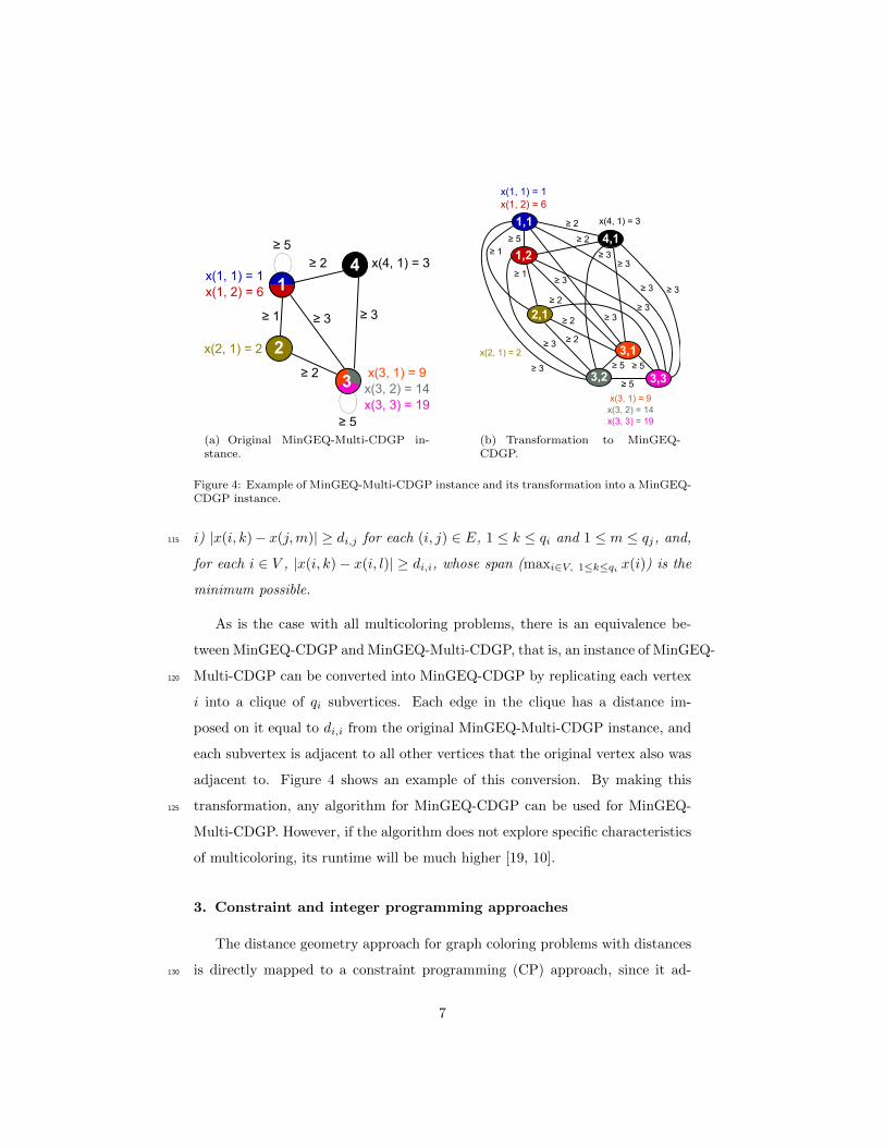
Figure 4: Example of MinGEQ-Multi-CDGP instance and its transformation into a MinGEQ-CDGP instance.

i) |x(i, k)− x(j,m)| ≥ di,j for each (i, j) ∈ E, 1 ≤ k ≤ qi and 1 ≤ m ≤ qj, and,115

for each i ∈ V , |x(i, k)− x(i, l)| ≥ di,i, whose span (maxi∈V, 1≤k≤qi x(i)) is the

minimum possible.

As is the case with all multicoloring problems, there is an equivalence be-

tween MinGEQ-CDGP and MinGEQ-Multi-CDGP, that is, an instance of MinGEQ-

Multi-CDGP can be converted into MinGEQ-CDGP by replicating each vertex120

i into a clique of qi subvertices. Each edge in the clique has a distance im-

posed on it equal to di,i from the original MinGEQ-Multi-CDGP instance, and

each subvertex is adjacent to all other vertices that the original vertex also was

adjacent to. Figure 4 shows an example of this conversion. By making this

transformation, any algorithm for MinGEQ-CDGP can be used for MinGEQ-125

Multi-CDGP. However, if the algorithm does not explore specific characteristics

of multicoloring, its runtime will be much higher [19, 10].

3. Constraint and integer programming approaches

The distance geometry approach for graph coloring problems with distances

is directly mapped to a constraint programming (CP) approach, since it ad-130

7

dresses the graph coloring problem with distances as an embedding of the graph

in one dimension, that is, a labeling of the vertices with natural numbers in-

dicating its projection on the line of real numbers, such that the distances of

the segments defined by the edge weights of the graph are met, and such that

the total range is minimized (the span of colors is minimized). In this way, a135

mathematical technique that handles these segments or distance constraints is

the desired, which happens through the constraint programming model. We

also present a traditional integer programming formulation, to compare both

approaches.

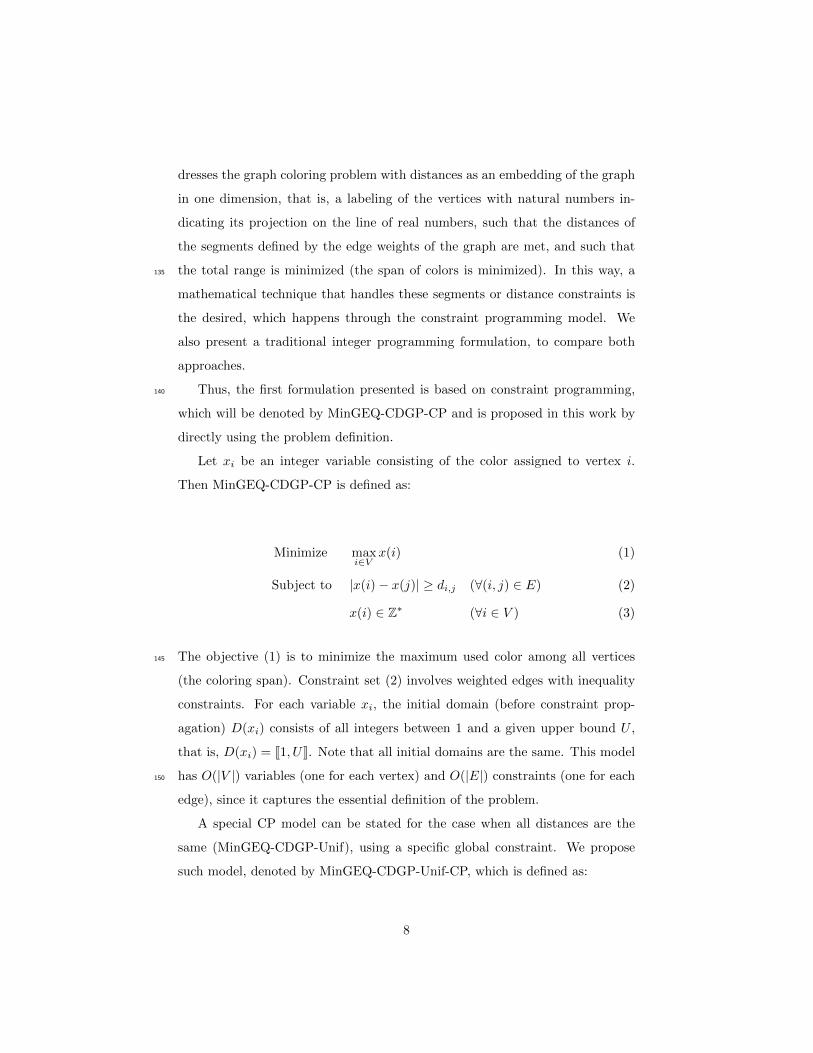
Thus, the first formulation presented is based on constraint programming,140

which will be denoted by MinGEQ-CDGP-CP and is proposed in this work by

directly using the problem definition.

Let xi be an integer variable consisting of the color assigned to vertex i.

Then MinGEQ-CDGP-CP is defined as:

Minimize maxi∈V

x(i) (1)

Subject to |x(i)− x(j)| ≥ di,j (∀(i, j) ∈ E) (2)

x(i) ∈ Z∗ (∀i ∈ V ) (3)

The objective (1) is to minimize the maximum used color among all vertices145

(the coloring span). Constraint set (2) involves weighted edges with inequality

constraints. For each variable xi, the initial domain (before constraint prop-

agation) D(xi) consists of all integers between 1 and a given upper bound U ,

that is, D(xi) = J1, UK. Note that all initial domains are the same. This model

has O(|V |) variables (one for each vertex) and O(|E|) constraints (one for each150

edge), since it captures the essential definition of the problem.

A special CP model can be stated for the case when all distances are the

same (MinGEQ-CDGP-Unif), using a specific global constraint. We propose

such model, denoted by MinGEQ-CDGP-Unif-CP, which is defined as:

8

Minimize maxi∈V

x(i) (4)

Subject to allMinDistance({x(j) : (i, j) ∈ E}, β) (∀i ∈ V ) (5)

x(i) ∈ Z∗ (∀i ∈ V ) (6)

The allMinDistance global constraint used in 5 takes as its arguments a set155

of variables and a constant w, and ensures that, for all pairs of variables y and z

in the set, the condition |y−z| ≥ w is valid, which is the case for each vertex and

its neighbors. This special case has O(|V |) variables and also O(|V |) constraints.

Since, for most connected graphs, we have |V | ≤ |E|, this formulation has fewer

constraints and is able to use specialized propagators in the search.160

For MinGEQ-Multi-CDGP, a CP formulation can be constructed by using

characteristics from both previously shown models. As discussed in Section 2,

a multicoloring problem can be converted into a coloring with single demands

by transforming a vertex i into a clique of qi vertices, each adjacent to all other

vertices that were adjacent to i. By using this, we have that, essentially, each165

vertex consists of a small MinGEQ-CDGP-Unif subinstance, where the larger

graph (that is, considering the constraints imposed on the original edges between

different vertices), if its multicoloring demands are ignored, is a MinGEQ-CDGP

instance. Based on this combination, we propose the following CP formulation,

denoted by MinGEQ-Multi-CDGP-CP:170

9

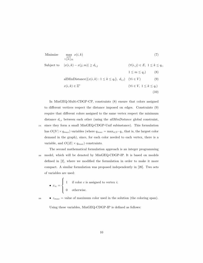
Minimize maxi∈V

1≤k≤qi

x(i, k) (7)

Subject to |x(i, k)− x(j,m)| ≥ di,j (∀(i, j) ∈ E, 1 ≤ k ≤ qi,

1 ≤ m ≤ qj) (8)

allMinDistance({x(i, k) : 1 ≤ k ≤ qi}, di,i) (∀i ∈ V ) (9)

x(i, k) ∈ Z∗ (∀i ∈ V, 1 ≤ k ≤ qi)

(10)

In MinGEQ-Multi-CDGP-CP, constraints (8) ensure that colors assigned

to different vertices respect the distance imposed on edges. Constraints (9)

require that different colors assigned to the same vertex respect the minimum

distance di,i between each other (using the allMinDistance global constraint,

since they form a small MinGEQ-CDGP-Unif subinstance). This formulation175

has O(|V |× qmax) variables (where qmax = maxi∈V ′ qi, that is, the largest color

demand in the graph), since, for each color needed to each vertex, there is a

variable, and O(|E| × qmax) constraints.

The second mathematical formulation approach is an integer programming

model, which will be denoted by MinGEQ-CDGP-IP. It is based on models180

defined in [2], where we modified the formulation in order to make it more

compact. A similar formulation was proposed independently in [20]. Two sets

of variables are used:

• xic =

1 if color c is assigned to vertex i;

0 otherwise.

• zmax = value of maximum color used in the solution (the coloring span).185

Using these variables, MinGEQ-CDGP-IP is defined as follows:

10

Minimize zmax (11)

Subject to

U∑c=1

xic = 1 (∀i ∈ V ) (12)

xic + xje ≤ 1 (∀(i, j) ∈ E; 1 ≤ c, e ≤ U | |c− e| < di,j) (13)

zmax ≥ cxic (∀i ∈ V ; 1 ≤ c ≤ U) (14)

xic ∈ {0, 1} (∀i ∈ V ; 1 ≤ c ≤ U) (15)

zmax ∈ R (16)

In MinGEQ-CDGP-IP, the objective (11) is to minimize the value of variable

zmax, which will be the coloring span. Constraint set (12) ensures that all

vertices must be colored. Constraint set (13) ensures that the absolute difference

between the colors assigned to adjacent vertices is less than the distance given by190

the weight of the respective edge, then only one of the vertices can receive that

color. Constraints (14) require that variable zmax be greater than or equal to

any color used, so it will be the maximum color used. Constraints (15) require

that variables in the set xic use only values 0 and 1, while constraint (16)

states that zmax is a free variable, although its value will always be an integer,195

since, at the optimal solution, zmax = cxic for some i ∈ V and c ∈ J1, UK.

The value U denotes the upper bound for colors to be used, since variables are

indexed by vertex and color, so the color set must be limited. This IP model has

O(U×|V |) variables (one for each pair of color and vertex) and O(U×(|E|+|V |))

constraints, that is, it has pseudopolynomial size.200

For MinGEQ-Multi-CDGP, the integer programming model can also be mod-

ified to accomodate multicoloring demands. We propose such formulation by

making two modifications must be made for the new model, which will be de-

noted as MinGEQ-Multi-CDGP-IP. The first one is changing the RHS of con-

straints (12) from 1 to qi, which ensures that, instead of receiving only one205

color, each vertex i will receive qi colors. The second one is expanding the set

11

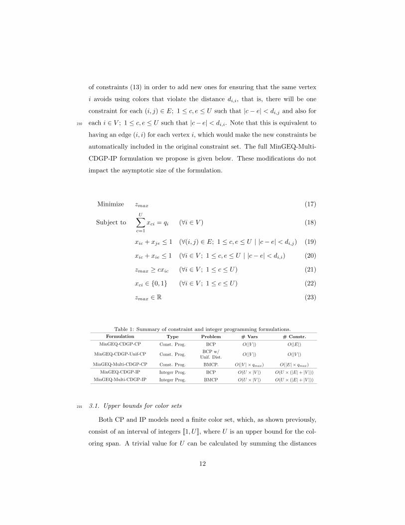
of constraints (13) in order to add new ones for ensuring that the same vertex

i avoids using colors that violate the distance di,i, that is, there will be one

constraint for each (i, j) ∈ E; 1 ≤ c, e ≤ U such that |c− e| < di,j and also for

each i ∈ V ; 1 ≤ c, e ≤ U such that |c− e| < di,i. Note that this is equivalent to210

having an edge (i, i) for each vertex i, which would make the new constraints be

automatically included in the original constraint set. The full MinGEQ-Multi-

CDGP-IP formulation we propose is given below. These modifications do not

impact the asymptotic size of the formulation.

Minimize zmax (17)

Subject to

U∑c=1

xci = qi (∀i ∈ V ) (18)

xic + xje ≤ 1 (∀(i, j) ∈ E; 1 ≤ c, e ≤ U | |c− e| < di,j) (19)

xic + xie ≤ 1 (∀i ∈ V ; 1 ≤ c, e ≤ U | |c− e| < di,i) (20)

zmax ≥ cxic (∀i ∈ V ; 1 ≤ c ≤ U) (21)

xci ∈ {0, 1} (∀i ∈ V ; 1 ≤ c ≤ U) (22)

zmax ∈ R (23)

Table 1: Summary of constraint and integer programming formulations.

Formulation Type Problem # Vars # Constr.

MinGEQ-CDGP-CP Const. Prog. BCP O(|V |) O(|E|)

MinGEQ-CDGP-Unif-CP Const. Prog.BCP w/

Unif. Dist.O(|V |) O(|V |)

MinGEQ-Multi-CDGP-CP Const. Prog. BMCP. O(|V | × qmax) O(|E| × qmax)

MinGEQ-CDGP-IP Integer Prog. BCP O(U × |V |) O(U × (|E|+ |V |))MinGEQ-Multi-CDGP-IP Integer Prog. BMCP O(U × |V |) O(U × (|E|+ |V |))

3.1. Upper bounds for color sets215

Both CP and IP models need a finite color set, which, as shown previously,

consist of an interval of integers J1, UK, where U is an upper bound for the col-

oring span. A trivial value for U can be calculated by summing the distances

12

imposed on all edges plus 1, that is, U =∑

(i,j)∈Edi,j + 1. However, this upper

bound is very weak, since, by summing all distances, we are ignoring the fact220

that colors can be reused by vertices not adjacent to each other, which makes

the coloring span become a large value far from optimum. This also makes the

color set have a large cardinality, which has a huge impact on the computing

performance of these models, especially the IP model, since the number of vari-

ables and constraints are proportional to the upper bound, which can lead to225

out-of-memory scenarios.

A better value for U is given by preprocessing the input graph, where an

heuristic which does not need an explicit upper bound is applied to it. The

span of the resulting solution is used as the value U when assembling CP and

IP models for the input graph. A greedy algorithm for coloring the input graph230

can be used for this, where the vertices are processed following an order based on

their color demands - vertices with higher demands are colored first. A color for

a vertice i is determined by first setting its color candidate as numCol[i]×di,i+1,

where numCol[i] is the number of colors already assigned to i, and checking if it

violates any separation constraint with any of its neighbor vertices. If a violation235

occurs, the color candidate is incremented by 1 and this checking is made again

until a feasible color is found. The color is then assigned to i and, if its demands

are not fully satisfied, an additional color is calculated and assigned to it. This is

repeated until the graph is fully colored. Algorithm 1 gives pseudocode for this

greedy heuristic. The upper bound is, then, the span of the solution returned240

by this method.

4. Computational experiments

The constraint and integer programming formulations were implemented in

C++ using IBM/ILOG CPLEX solver, version 12.5.1, and its CP Optimizer

component. The resulting programs were executed in a Microsoft Azure A9245

Virtual Machine, consisting of Intel Xeon E5-2670 processors (16 cores @ 2.6

GHz), 112GB of RAM and Ubuntu Linux 14.04.1 LTS operating system. Both

13

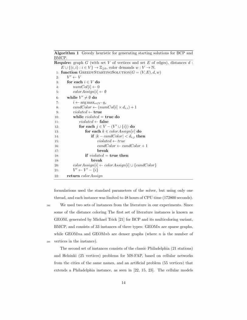
Algorithm 1 Greedy heuristic for generating starting solutions for BCP andBMCP.Require: graph G (with set V of vertices and set E of edges), distances d :

E ∪ {(i, i) : i ∈ V } → Z≥0, color demands w : V → N.1: function GreedyStartingSolution(G = (V,E), d, w)2: V ′ ← V3: for each i ∈ V do4: numCol[i]← 05: colorAssign[i]← ∅6: while V ′ 6= ∅ do7: i← arg maxv∈V ′ qv8: candColor ← (numCol[i]× di,i) + 19: violated← true

10: while violated = true do11: violated← false12: for each j ∈ V − (V ′ ∪ {i}) do13: for each k ∈ colorAssign[v] do14: if |k − candColor| < di,j then15: violated← true16: candColor ← candColor + 117: break18: if violated = true then19: break20: colorAssign[i]← colorAssign[i] ∪ {candColor}21: V ′ ← V ′ − {i}22: return colorAssign

formulations used the standard parameters of the solver, but using only one

thread, and each instance was limited to 48 hours of CPU time (172800 seconds).

We used two sets of instances from the literature in our experiments. Since250

some of the distance coloring The first set of literature instances is known as

GEOM, generated by Michael Trick [21] for BCP and its multicoloring variant,

BMCP, and consists of 33 instances of three types: GEOMn are sparse graphs,

while GEOMna and GEOMnb are denser graphs (where n is the number of

vertices in the instance).255

The second set of instances consists of the classic Philadelphia (21 stations)

and Helsinki (25 vertices) problems for MS-FAP, based on cellular networks

from the cities of the same names, and an artificial problem (55 vertices) that

extends a Philadelphia instance, as seen in [22, 15, 23]. The cellular models

14

1 32 4 56 7 8 9 10 11 12

13 14 15 16 17 1819 20 21

(a) Philadelphia.

1 32 4 5 67 8 9 10 11 12

15 16 17 18 19 20 21

13 14

22 23 24 25 26 27 28 2930 31 32 33 34 35 36 37 38

39 40 41 42 43 44 45 46 4748 49 50 51 52 53 54 55

(b) Artificial.

Figure 5: Examples of instances for MinGEQ-CDGP (BCP) and MinGEQ-CDGP-Unif prob-lems. Note that the MinGEQ-CDGP-Unif instance used is a classic graph coloring problem.

(hexagonal cells) for Philadelphia and artificial instances are given in Figure260

Since these instances are defined for BMCP only, we applied the suggestion by

the authors of the GEOM instances in these as well to generate BCP instances.

When constructing the models for each instance, we executed the prepro-

cessing discussed in Subsection 3.1 in order to obtain a feasible solution and an

upper bound. To further help the solvers, we fed the entire starting solution to265

them, namely, we passed the solution as a starting point to CP Optimizer and

as a MIP start to CPLEX, instead of only using the span as an upper bound.

This is especially important for CPLEX, since it guarantees that an optimality

gap is calculated as soon as the enumeration starts.

The first results presented are for BCP. Table 2 shows the results for the270

GEOM BCP instances. Since the BCP variants are also used in the literature,

we compared our results with the Discropt heuristic framework in [7] and the

multistart iterated tabu search heuristic in [10] to verify the correctness of the

solutions by the CP and IP formulations. For all sparse instances (the ones

without ’a’ or ’b’ in the name), the constraint programming implementation275

was able to prove optimality. However, we emphasize that, for some instances,

no method achieved the best solution presented in [7]. As noted in [10], no

other work has obtained the same results, while our exact approaches reached

the same best solutions for these instances obtained by other authors, which

leads us to believe there is a mistake in [7], as marked in Table 2.280

15

Time limit (48h) Time limit (48h)

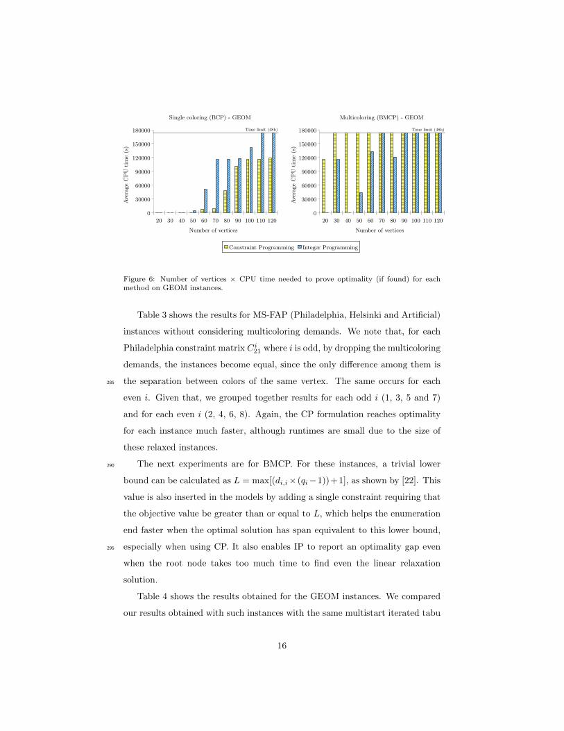
Figure 6: Number of vertices × CPU time needed to prove optimality (if found) for eachmethod on GEOM instances.

Table 3 shows the results for MS-FAP (Philadelphia, Helsinki and Artificial)

instances without considering multicoloring demands. We note that, for each

Philadelphia constraint matrix Ci21 where i is odd, by dropping the multicoloring

demands, the instances become equal, since the only difference among them is

the separation between colors of the same vertex. The same occurs for each285

even i. Given that, we grouped together results for each odd i (1, 3, 5 and 7)

and for each even i (2, 4, 6, 8). Again, the CP formulation reaches optimality

for each instance much faster, although runtimes are small due to the size of

these relaxed instances.

The next experiments are for BMCP. For these instances, a trivial lower290

bound can be calculated as L = max[(di,i× (qi−1))+1], as shown by [22]. This

value is also inserted in the models by adding a single constraint requiring that

the objective value be greater than or equal to L, which helps the enumeration

end faster when the optimal solution has span equivalent to this lower bound,

especially when using CP. It also enables IP to report an optimality gap even295

when the root node takes too much time to find even the linear relaxation

solution.

Table 4 shows the results obtained for the GEOM instances. We compared

our results obtained with such instances with the same multistart iterated tabu

16

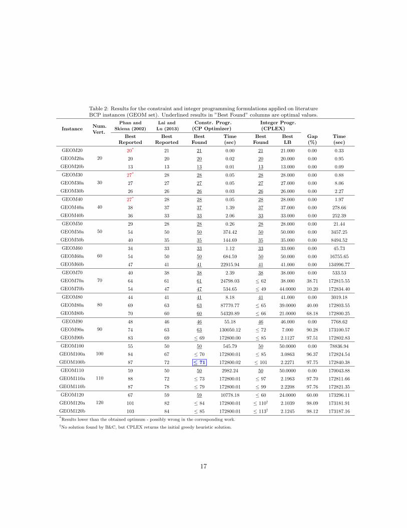
Table 2: Results for the constraint and integer programming formulations applied on literatureBCP instances (GEOM set). Underlined results in ”Best Found” columns are optimal values.

InstanceNum.Vert.

Phan and

Skiena (2002)

Lai and

Lu (2013)

Constr. Progr.(CP Optimizer)

Integer Progr.(CPLEX)

BestReported

BestReported

BestFound

Time(sec)

BestFound

BestLB

Gap(%)

Time(sec)

GEOM20

20

20* 21 21 0.00 21 21.000 0.00 0.33

GEOM20a 20 20 20 0.02 20 20.000 0.00 0.95

GEOM20b 13 13 13 0.01 13 13.000 0.00 0.09

GEOM30

30

27* 28 28 0.05 28 28.000 0.00 0.88

GEOM30a 27 27 27 0.05 27 27.000 0.00 8.06

GEOM30b 26 26 26 0.03 26 26.000 0.00 2.27

GEOM40

40

27* 28 28 0.05 28 28.000 0.00 1.97

GEOM40a 38 37 37 1.39 37 37.000 0.00 278.66

GEOM40b 36 33 33 2.06 33 33.000 0.00 252.39

GEOM50

50

29 28 28 0.26 28 28.000 0.00 21.44

GEOM50a 54 50 50 374.42 50 50.000 0.00 3457.25

GEOM50b 40 35 35 144.69 35 35.000 0.00 8494.52

GEOM60

60

34 33 33 1.12 33 33.000 0.00 45.73

GEOM60a 54 50 50 684.59 50 50.000 0.00 16755.65

GEOM60b 47 41 41 22915.94 41 41.000 0.00 134996.77

GEOM70

70

40 38 38 2.39 38 38.000 0.00 533.53

GEOM70a 64 61 61 24798.03 ≤ 62 38.000 38.71 172815.55

GEOM70b 54 47 47 534.65 ≤ 49 44.0000 10.20 172834.40

GEOM80

80

44 41 41 8.18 41 41.000 0.00 3019.18

GEOM80a 69 63 63 87770.77 ≤ 65 39.0000 40.00 172803.55

GEOM80b 70 60 60 54320.89 ≤ 66 21.0000 68.18 172800.25

GEOM90

90

48 46 46 55.18 46 46.000 0.00 7768.62

GEOM90a 74 63 63 130050.12 ≤ 72 7.000 90.28 173100.57

GEOM90b 83 69 ≤ 69 172800.00 ≤ 85 2.1127 97.51 172802.83

GEOM100

100

55 50 50 545.79 50 50.0000 0.00 78836.94

GEOM100a 84 67 ≤ 70 172800.01 ≤ 85 3.0863 96.37 172824.54

GEOM100b 87 72 ≤ 71 172800.02 ≤ 101 2.2271 97.75 172840.38

GEOM110

110

59 50 50 2982.24 50 50.0000 0.00 170043.88

GEOM110a 88 72 ≤ 73 172800.01 ≤ 97 2.1963 97.70 172811.66

GEOM110b 87 78 ≤ 79 172800.01 ≤ 99 2.2208 97.76 172821.35

GEOM120

120

67 59 59 10778.18 ≤ 60 24.0000 60.00 173296.11

GEOM120a 101 82 ≤ 84 172800.01 ≤ 110† 2.1039 98.09 173181.91

GEOM120b 103 84 ≤ 85 172800.01 ≤ 113† 2.1245 98.12 173187.16*Results lower than the obtained optimum - possibly wrong in the corresponding work.

†No solution found by B&C, but CPLEX returns the initial greedy heuristic solution.

17

Table 3: Results for the constraint and integer programming formulations applied on litera-ture MS-FAP instances (Philadelphia, Helsinki and Artificial) without multicoloring demands.Since IP reaches all optimal solutions, the best LB has been omitted in the table.

Const. matrixNum.Vert.

Constr. Progr.(CP Optimizer)

Integer Progr.(CPLEX - B&C)

BestFound

Time(sec)

BestFound

Time(sec)

C121, C3

21, C521 and C7

2121

7 0.40 7 0.87

C221, C4

21, C621 and C8

21 9 0.06 9 2.66

C125 25 8 4.71 8 1.90

C155 55 7 0.79 7 30.63

search heuristic from [10], where the algorithm for BCP is applied to BMCP300

instances by expanding the vertices into cliques as shown in Section 2, and also

with the general purpose heuristic system (Discropt) used in [7]. We also used

the MS-FAP (Philadelphia, Helsinki and Artificial) instances in their original

forms (that is, including multicoloring) and compared with the constructive

heuristic from [22], the local search algorithm from [23] and the memetic algo-305

rithm from [24].

For BMCP, the efficiency between CP and IP is practically reversed: most in-

stances are solved to optimality faster with IP than CP. In fact, for the MS-FAP

instances, we were able to obtain all optimal values using IP. This is explained

by taking into account, as discussed in Section 3, that the IP model is able to310

consider multicoloring demands without expanding the number of vertices, only

having to change a set of constraints and add another set for the different colors

for each vertex. However, the CP model has to grow more, since, essentially, a

BMCP instance is treated as a special BCP one, since the number of variables

increases and a new set of constraints is introduced. Figure 6 shows this dif-315

ference in efficiency between methods. However, CP still has an advantage in

BMCP: when it is unable to solve a problem to optimality in the given time

limit, the solution that it returns has a better quality than the one found by IP

(that is, the coloring span of the solution found by CP is lower than the one

found by IP). This happens because CP has explicit information about which320

colors each vertex can assume, instead of calculating such colors.

18

We also detected a mistake in [22], where the heuristic result presented in

it for constraint matrix C125 and demand vector D4

25 is better (with objective

function value 121) than the exact solutions obtained by both CP and IP (with

objective function value 200). In fact, no other work in the literature obtained325

a solution with span lower than 200.

Table 4: Results for the constraint and integer programming formulations applied on literatureBMCP instances (GEOM set).

InstanceNum.Vert.

TrivialLB

Lai and

Lu (2013)

Constr. Progr.(CP Optimizer)

Integer Progr.(CPLEX - B&C)

BestReported

BestFound

Time(sec)

BestFound

BestLB

Gap(%)

Time(sec)

GEOM20

20

91 149 ≤ 149 172800.01 149 149.0000 0.00 15.17

GEOM20a 91 169 ≤ 169 172800.01 169 169.0000 0.00 18.49

GEOM20b 21 44 44 476.92 44 44.0000 0.00 1.58

GEOM30

30

91 160 ≤ 160 172800.01 ≤ 160 159.0000 0.62 172830.72

GEOM30a 91 209 ≤ 215 172800.01 ≤ 211 189.0000 10.43 172813.47

GEOM30b 21 77 ≤ 77 172800.00 77 77.0000 0.00 41.87

GEOM40

40

91 167 ≤ 168 172800.01 167 167.0000 0.00 1192.28

GEOM40a 91 213 ≤ 225 172800.01 213 213.0000 0.00 111262.08

GEOM40b 21 74 ≤ 74 172800.00 74 74.0000 0.00 17027.77

GEOM50

50

91 224 ≤ 226 172800.02 224 224.0000 0.00 52450.85

GEOM50a 91 314 ≤ 332 172800.03 ≤ 361 95.5218 73.54 172820.13

GEOM50b 21 83 ≤ 85 172800.00 ≤ 87 52.0000 40.23 172819.47

GEOM60

60

91 258 ≤ 259 172800.02 258 258.0000 0.00 156987.80

GEOM60a 91 356 ≤ 380 172800.03 ≤ 448 93.5801 78.93 172813.01

GEOM60b 21 113 ≤ 117 172800.01 ≤ 125 34.0000 72.80 172897.07

GEOM70

70

91 270 ≤ 284 172800.03 ≤ 305 94.2092 69.11 172804.56

GEOM70a 91 467 ≤ 483 172800.05 ≤ 578 91.0000 84.26 172839.51

GEOM70b 21 116 ≤ 123 172800.01 ≤ 134 22.7359 83.03 172805.88

GEOM80

80

91 381 ≤ 395 172800.04 ≤ 511 95.2644 80.19 172809.70

GEOM80a 91 361 ≤ 382 172800.05 ≤ 479 91.0000 81.00 172885.02

GEOM80b 21 139 ≤ 145 172800.01 ≤ 170 23.0547 86.44 172820.56

GEOM90

90

91 330 ≤ 342 172800.05 ≤ 423 93.2736 77.73 172811.82

GEOM90a 91 375 ≤ 392 172800.07 ≤ 452 91.0000 79.87 172830.60

GEOM90b 21 144 ≤ 156 172800.01 ≤ 212 22.2574 89.50 172844.07

GEOM100

100

91 404 ≤ 426 172800.07 ≤ 493 94.2797 80.88 173190.69

GEOM100a 91 442 ≤ 465 172800.08 ≤ 596 91.0000 84.73 172871.84

GEOM100b 21 156 ≤ 169 172800.02 ≤ 220 21.0000 90.45 172810.33

GEOM110

110

91 381 ≤ 399 172800.07 ≤ 500 91.0000 81.80 172840.98

GEOM110a 91 488 ≤ 527 172800.10 ≤ 610 91.0000 85.08 173095.42

GEOM110b 21 204 ≤ 207 172800.01 ≤ 250 22.0001 91.20 172835.82

GEOM120

120

91 396 ≤ 427 172800.06 ≤ 505 93.9762 81.39 172923.18

GEOM120a 91 554 ≤ 585 172800.16 ≤ 641 91.0000 85.80 173312.14

GEOM120b 21 189 ≤ 202 172800.01 ≤ 247 21.8723 91.14 172852.82

19

Table 5: Results for the constraint and integer programming formulations applied on litera-ture MS-FAP instances (Philadelphia, Helsinki and Artificial). Since IP reaches all optimalsolutions, the best LB has been omitted in the table.

Const.matr.

Demd.vect.

Num.Vert.

LowerBound

Chakraborty

(2001)

Kendall and

Mohamad

(2005)

Kim et al.

(2007)

Constr. Progr.(CP Optimizer)

Integer Progr.(CPLEX - B&C)

BestReported

BestReported

BestReported

BestFound

Time(sec)

BestFound

Time(sec)

C121 D1

21

21

533 533 533 533 533 4.20 533 0.50

C121 D2

21 309 309 309 309 309 1.34 309 1.22

C221 D1

21 533 533 533 533 533 10.53 533 308.04

C221 D2

21 309 309 309 309 309 625.93 309 165.54

C321 D1

21 457 457 457 – 457 3.96 457 0.39

C321 D2

21 265 265 265 – 265 3.54 265 1.52

C421 D1

21 457 457 457 – 457 41.24 457 202.01

C421 D2

21 265 265 265 – ≤ 266 172800.06 265 214.01

C521 D1

21 381 381 381 381 381 3.23 381 0.29

C521 D2

21 221 221 221 221 221 100.81 221 5.09

C621 D1

21 381 463 435 427 ≤ 449 172800.08 427 6827.49

C621 D2

21 221 273 268 253 ≤ 266 172800.04 253 2026.67

C721 D1

21 305 305 305 – 305 12.85 305 1.10

C721 D2

21 177 197 185 – ≤ 180 172800.06 180 24.54

C821 D1

21 305 465 444 – ≤ 435 172800.07 427 1185.27

C821 D2

21 177 278 271 – ≤ 267 172800.06 253 1116.45

C125 D3

25 2521 73 73 – ≤ 73 172800.00 73 1.10

C125 D4

25 89 121* 200 – ≤ 200 172800.07 200 2.18

C155 D5

55 55309 309 309 – 309 11078.95 309 460.12

C155 D6

55 71 79 72 – 71 6.33 71 28.56*Results lower than the obtained optimum - possibly wrong in the corresponding work.

Finally, the numbers of branches and paths that do not reach a solution in

the CP enumeration and generated cuts of each type in the IP enumeration are

given in Tables 6 and 7 for instances with unit color demands and in Tables

Tables 8 and 9 for instances with multicoloring demands. We note that there is330

not a clear correlation between the instance size and this data, indicating that

these parts of the algorithms are sensitive to the individual values of distances

and demands in the instances. We also conjecture that the input graph layout

also impacts in the enumeration, since some known cuts applied to coloring

problems, such as clique cuts [25], are derived according to the graph to be335

colored.

20

Table 6: Number of branches and fails (for CP) and of global cuts of each type (for IP) appliedto GEOM instances with unit demands.

InstanceNum.Vert.

Const. Prog. (CP Optimizer) Integer Progr. (CPLEX)

# Branches # Fails# Clique

Cuts

# ImpliedBoundCuts

# MIPRounding

Cuts

#Zero-Half

Cuts

# GomoryFractional

Cuts

GEOM20

20

972 462 9 15 0 8 10

GEOM20a 4667 2298 3 27 0 2 9

GEOM20b 2224 1096 14 7 0 5 0

GEOM30

30

10102 4782 13 62 0 4 31

GEOM30a 9024 4353 25 473 0 20 60

GEOM30b 6651 3210 9 194 0 11 49

GEOM40

40

9965 4699 13 130 0 3 56

GEOM40a 206960 98635 43 4 117 3 1

GEOM40b 275519 131721 14 543 0 30 15

GEOM50

50

57869 27159 27 0 0 9 0

GEOM50a 40966958 19591854 227 13 138 12 0

GEOM50b 14438962 6973218 564 3 6 18 0

GEOM60

60

178478 82471 63 0 0 0 2

GEOM60a 59350249 28292260 241 19 182 28 24

GEOM60b 1700740733 807817043 1691 25 176 23 0

GEOM70

70

320560 148877 128 0 12 3 1

GEOM70a 1662200599 781294815 881 6 192 20 0

GEOM70b 301138496 143985463 1171 21 226 46 5

GEOM80

80

2173324 1008986 372 5 131 19 0

GEOM80a 8859155916 4149659761 761 30 389 85 5

GEOM80b 3687195162 1739030200 480 29 303 138 0

GEOM90

90

3841482 1748958 471 2 223 31 9

GEOM90a 8424930433 3953124503 143 3 411 349 0

GEOM90b 6454145085 3036820947 317 11 417 93 0

GEOM100

100

33141115 15198269 702 11 221 54 27

GEOM100a 6622094014 3084753118 330 2 1367 2162 245

GEOM100b 5409742123 2511274478 130 301 0 567 136

GEOM110

110

12496119255 5760860721 426 16 320 54 2

GEOM110a 5930484572 2724545532 151 501 0 619 79

GEOM110b 4177753606 1922426902 118 754 0 460 0

GEOM120

120

637959908 289378147 1015 19 357 128 8

GEOM120a 5560296354 2542244856 172 782 0 678 0

GEOM120b 4003420813 1841115383 273 1258 0 959 0

Table 7: Number of branches and fails (for CP) and of global cuts of each type (for IP) appliedto MS-FAP instances (Philadelphia, Helsinki and Artificial) without multicoloring demands.

InstanceNum.Vert.

Const. Prog. (CP Optimizer) Integer Progr. (CPLEX)

# Branches # Fails# Clique

Cuts

# ImpliedBoundCuts

# MIPRounding

Cuts

#Zero-Half

Cuts

# GomoryFractional

Cuts

C121, C3

21, C521 and C7

2121

49177 24602 3 5 0 9 0

C221, C4

21, C621 and C8

21 6033 2970 5 5 0 58 3

C125 25 176565 87496 0 0 0 0 0

C155 55 49096 24214 0 0 0 0 0

21

Table 8: Number of branches and fails (for CP) and of global cuts of each type (for IP) appliedto GEOM instances with multicoloring demands.

InstanceNum.Vert.

Const. Prog. (CP Optimizer) Integer Progr. (CPLEX)

# Branches # Fails# Clique

Cuts

# ImpliedBoundCuts

# MIPRounding

Cuts

#Zero-Half

Cuts

# GomoryFractional

Cuts

GEOM20

20

1847656377 823996186 26 33 0 22 0

GEOM20a 2060224899 926128135 35 378 0 92 91

GEOM20b 23433594 11236673 19 28 0 47 49

GEOM30

30

1594445634 702092983 345 1 7 29 0

GEOM30a 778845728 343378790 1234 6 189 3 0

GEOM30b 4336696005 2043720645 23 96 0 17 53

GEOM40

40

1101215203 477955956 186 287 0 158 0

GEOM40a 853750393 376905743 131 7 322 4 0

GEOM40b 2915214186 1378502269 361 1 4 2 0

GEOM50

50

858223844 366277155 575 0 79 31 0

GEOM50a 373860395 159472193 183 446 0 235 4

GEOM50b 2205618883 1031493835 1498 2 295 7 0

GEOM60

60

884613825 374341633 468 1 34 38 0

GEOM60a 327100218 135221648 1109 335 0 1213 0

GEOM60b 1625337918 741993923 143 3 456 7 0

GEOM70

70

480579106 200225715 497 1363 0 275 0

GEOM70a 178618063 71625162 0 0 0 0 0

GEOM70b 1153010252 520892432 133 2 645 165 29

GEOM80

80

491579072 131225337 786 1842 0 1343 85

GEOM80a 206713326 84260206 0 0 0 0 0

GEOM80b 972753631 434139515 328 1065 0 690 97

GEOM90

90

289804704 110251804 1321 0 0 1894 0

GEOM90a 203904382 82252836 0 0 0 0 0

GEOM90b 677312582 300211365 344 481 0 877 0

GEOM100

100

219953270 80390988 0 0 0 0 0

GEOM100a 134018202 52245146 0 0 0 0 0

GEOM100b 511570190 224573165 0 0 0 0 0

GEOM110

110

170668054 64299043 0 0 0 0 0

GEOM110a 113908674 41331333 0 0 0 0 0

GEOM110b 409339582 177985395 0 0 0 0 0

GEOM120

120

207980564 81060477 0 0 0 0 0

GEOM120a 82058712 30432596 0 0 0 0 0

GEOM120b 386743755 164997551 0 0 0 0 0

22

Table 9: Number of branches and fails (for CP) and of global cuts of each type (for IP) appliedto MS-FAP instances (Philadelphia, Helsinki and Artificial).

Const.Matr.

Demd.Vect.

Num.Vert.

Const. Prog. (CP Optimizer) Integer Progr. (CPLEX)

# Branches # Fails# Clique

Cuts

# ImpliedBoundCuts

# MIPRounding

Cuts

#Zero-Half

Cuts

# GomoryFractional

Cuts

C121 D1

21

21

2555 504 0 0 0 0 0

C121 D2

21 469 4 0 0 0 0 0

C221 D1

21 6610 1505 0 0 0 0 0

C221 D2

21 822377 309790 0 0 0 0 0

C321 D1

21 2451 504 0 0 0 0 0

C321 D2

21 2874 505 0 0 0 0 0

C421 D1

21 20982 5811 0 0 0 0 0

C421 D2

21 44845827 17108454 0 0 0 0 0

C521 D1

21 2305 504 0 0 0 0 0

C521 D2

21 158368 50239 0 0 0 0 0

C621 D1

21 180812651 65917318 160 4 210 116 0

C621 D2

21 347622756 121153772 170 1 37 159 0

C721 D1

21 4106 505 0 0 0 0 0

C721 D2

21 352244757 132070514 4 0 0 8 35

C821 D1

21 199948906 75399919 163 1 379 224 0

C821 D2

21 451729822 146753868 225 204 0 190 0

C125 D3

25 252435656356 1064961796 2 134 0 81 143

C125 D4

25 374343491 115700707 0 0 0 0 0

C155 D5

55 557809104 2371461 0 0 0 0 0

C155 D6

55 27897 9552 0 0 0 0 0

5. Concluding remarks

In this paper, we addressed channel assignment in wireless networks as spe-

cial graph coloring with distance constraints, and explored some feasibility prop-

erties on them, by proving some specific graph classes which admit or do not340

admit solutions. The special coloring problems with distance constraints were

modeled by distance geometry being considered as the general problem. We

have assigned the vertices on the real line, according to the distances between

adjacent vertices. Beyond that, we have described feasibility conditions for some

classes of graphs.345

We employed constraint and integer programming formulations, which were

implemented using computational OR tools, and applied them to instances from

the literature and new random ones in order to verify which mathematical mod-

eling tool is best for these distance coloring models. Since the constraints from

the problems are naturally transported to constraint programming, its imple-350

23

mentation reaches the optimal solution much faster than the integer program-

ming one.

Ongoing and future works include improving the CP formulation by domain

reduction and more specific constraints, and also use hybrid methods, combining

both CP and IP, as well as heuristics, in order to solve the distance coloring355

models faster. The study of the problems posed to specific classes of graphs,

in order to establish the characterization of feasibility conditions for them, is

subject of the research in progress.

References

[1] R. Karp, Reducibility Among Combinatorial Problems, in: R. E. Miller,360

J. W. Thatcher (Eds.), Complexity of Computer Computations, Plenum

Press, 1972, pp. 85–103.

[2] A. Koster, Frequency assignment: models and algorithms, Ph.D. thesis,

Universiteit Maastricht, the Netherlands (1999).

[3] G. Audhya, K. Sinha, S. Ghosh, B. Sinha, A survey on the channel assign-365

ment problem in wireless networks, Wireless Communications and Mobile

Computing 11 (2011) 583–609.

[4] K. Gokbayrak, E. A. Yıldırım, Joint gateway selection, transmission slot

assignment, routing and power control for wireless mesh networks, Com-

puters & Operations Research 40 (7) (2013) 1671–1679.370

[5] W. Hale, Frequency assignment: Theory and applications, Proceedings of

the IEEE 25 (1980) 1497–1514.

[6] R. Dorne, J. Hao, Tabu search for graph coloring, t-coloring and set t-

colorings, in: S. Voss, S. Martello, I. Osman, C. Roucairol (Eds.), Meta-

heuristics: advances and trends in local search paradigms for optimization,375

Kluver Academic Publishers, 1998, pp. 77–92.

24

[7] V. Phan, S. Skiena, Coloring graphs with a general heuristic search engine,

in: Computational Symposium on Graph Coloring and Its Generalizations,

2002, pp. 92–99.

[8] E. Malaguti, P. Toth, An evolutionary approach for bandwidth multicol-380

oring problems, European Journal of Operational Research 189 (3) (2008)

638–651. doi:10.1016/j.ejor.2006.09.095.

[9] E. Malaguti, P. Toth, A survey on vertex coloring problems, International

Transactions in Operational Research 17 (1) (2010) 1–34. doi:10.1111/

j.1475-3995.2009.00696.x.385

[10] X. Lai, Z. Lu, Multistart Iterated Tabu Search for Bandwidth Coloring

Problem, Computers & Operations Research 40 (2013) 1401–1409.

[11] B. Dias, Theoretical models and algorithms for optimizing channel assign-

ment in wireless mobile networks, Master’s thesis, Federal University of

Amazonas, Brazil, in portuguese (2014).390

[12] B. Dias, R. Freitas, J. Szwarcfiter, On graph coloring problems with dis-

tance constraints, in: Proceedings of I Workshop on Distance Geometry

and Applications (DGA 2013), 2013.

[13] B. Dias, R. Freitas, N. Maculan, Alocacao de canais em redes celulares sem

fio: algoritmos e modelos teoricos em grafos e escalonamento, in: Proceed-395

ings of the XVI Latin-Ibero-American Conference on Operations Research

/ XLIV Brazilian Symposium of Operations Research, Brazilian Society of

Operations Research (SOBRAPO), 2012, in portuguese.

[14] D. Costa, On the use of some known methods for T-coloring of graphs,

Annals of Operations Research 41 (1999) 343–358.400

[15] B. Dias, R. Freitas, N. Maculan, Simulated annealing para a alocacao de

canais em redes moveis celulares, in: Proceedings of the XLV Brazilian

Symposium on Operations Research, Sociedade Brasileira de Pesquisa Op-

eracional (SOBRAPO), 2013, in portuguese.

25

[16] P. Galinier, A. Hertz, A survey of local search methods for graph coloring,405

Computers & Operations Research 33 (2006) 2547–2562.

[17] C. Lavor, L. Liberti, N. Maculan, A. Mucherino, The discretizable molecu-

lar distance geometry problem, European Journal of Operational Research

52 (1) (2012) 115–146.

[18] B. Dias, R. de Freitas, N. Maculan, J. Szwarcfiter, Distance geometry ap-410

proach for special graph coloring problems, International Transactions in

Operational Research (submitted, 2015).

[19] A. Mehrotra, M. A. Trick, A Branch-And-Price Approach for Graph Multi-

Coloring, in: E. Baker, A. Joseph, A. Mehrotra, M. A. Trick (Eds.), Ex-

tending the Horizons: Advances in Computing, Optimization, and Decision415

Technologies, Vol. 37 of Operations Research/Computer Science Interfaces

Series, Springer, 2007, pp. 15–29.

[20] V. Mak, Polyhedral studies for minimum-span graph labelling with integer

distance constraints, International Transactions in Operational Research

14 (2) (2007) 105–121. doi:10.1111/j.1475-3995.2007.00577.x.420

[21] M. Trick, A. Mehrotra, D. Johnson, COLOR02/03/04: Graph Coloring

and its Generalizations, http://mat.gsia.cmu.edu/COLOR02/ (2002).

[22] G. Chakraborty, An Efficient Heuristic Algorithm for Channel Assignment

Problem in Cellular Radio Networks, IEEE Transactions on Vehicular Tech-

nology 50 (6) (2001) 1528–1539.425

[23] G. Kendall, M. Mohamad, Solving the Fixed Channel Assignment Problem

in Cellular Communications Using an Adaptive Local Search, in: E. Burke,

M. Trick (Eds.), 5th International Conference for the Practice and Theory

of Automated Timetabling (PATAT 2004), Lecture Notes in Computer

Science, vol. 3616, Springer, Heidelberg, 2005.430

26

[24] S.-S. Kim, A. E. Smith, J.-H. Lee, A memetic algorithm for channel as-

signment in wireless {FDMA} systems, Computers & Operations Research

34 (6) (2007) 1842 – 1856.

[25] I. Mendez-Dıaz, P. Zabala, A Branch-and-Cut algorithm for graph coloring,

Discrete Applied Mathematics 154 (2006) 826–847.435

27