FLUID DYNAMICS OF LITHIUM ION BATTERY VENTINGFAILURES

by

FRANK AUSTIN MIER

Submitted in Partial Fulfillmentof the Requirements for the Degree of

Doctor of Philosophy in Mechanical Engineeringwith Dissertation in Intelligent Energetic Systems

New Mexico Institute of Mining and TechnologySocorro, New Mexico

August, 2020

ABSTRACT

Lithium batteries have a well documented tendency to fail violently un-der abuse conditions which can result in venting of flammable and otherwisehazardous material. The 18650 format batteries of interest here have a perforatedvent cap incorporated in the positive terminal which is designed to burst beforefull case rupture under pressure build up. Here, the fluid dynamics of vent-initiated failures is considered from pressure build up during thermal runawayto the subsequent pressure driven venting flow. The characterization of the fail-ures leads to improved safety for identifying cell failures and the impact on thesurrounding environment. Increasing the basic understanding of venting flowslinks internal battery hazards and the safety of the surrounding environment.

Battery case strain and temperature were measured on cells under thermalabuse which was used to calculate internal pressure via hoop and longitudinalstress relations. Strain measurement is a non-invasive approach with no impacton the chemical decomposition within batteries that leads to thermal runaway.The experimental methodology and test apparatus were developed and validatedthrough predictable, representative test specimens of open cases and pressurizedgas cylinders. Live battery experiments reliably captured the final pressure risebefore venting onset. The pressure build up was observed to coincide with thebeginning of thermal runaway.

Vented material leaves the battery cells as a complex multiphase, reactiveflow. Experiments were performed to address droplet spray and interactions be-tween nearby, steady gas jets representative of actual battery vents. Battery ventswere pressurized until failure with carbon dioxide and sucrose solution to repre-sent electrolyte. High speed schlieren imaging visualized the droplet spray andsurrounding gas flow immediately after burst. The resulting droplet spray wasfound to vary in characteristics depending on the fluid dynamic properties ofthe liquid material. The resulting droplet flow spreads to angles wider than thegaseous portions of the jet and are projected into the atmosphere. Image process-ing methods were developed to extract droplet flow paths from the gas jets.

In the 18650 battery vent cap studied here, venting consists of four indi-vidual jets. Fundamental fluid dynamic experiments were developed to study theinteraction between nearby gas jets, in a simplified geometry of two outwardlyoriented gas jets issuing into a quiescent environment. Particle Image Velocime-try (PIV) measured the interaction between the jets which was quantified in termsof mean velocity and turbulence strength profiles. A semi-analytical model wasdeveloped to predict the combined jet velocity profiles and interactions. Jets ofsmall offset angles and orifice spacings demonstrated greater interaction in the

i

combined flow field, and jets oriented outward at angles of more than 20° wereobserved to not interact. Results of the experiments identify the flow field cre-ated during vent failures which can be used to validate or enhance simulationsof mixing during venting failures and the evolution of the potentially flammableenvironment created outside of the cell. The work presented here provides quan-tifications to the broad scenario of venting flows which assists the characteriza-tion of battery failures.

Keywords: Lithium ion battery; Safety; Venting failure; Internal pressure; Jetinteraction

ii

ACKNOWLEDGMENTS

I would like to thank research advisor Dr. Michael J. Hargather for hisguidance and expertise throughout this and previous work. I am grateful forthe research experiences I have had with the Shock and Gas Dynamics Labo-ratory since I joined the lab as an undergraduate student. The research in Dr.Hargather’s lab from all students has been captivating, and I look forward tofinishing my graduate studies here.

Funding from Dr. Summer Ferreira and Dr. Joshua Lamb at Sandia Na-tional Laboratories under PO 1989037, PO 1859922, and PO 1739875 has madethis research possible over the past 4 years. Dr. Ferreira and Dr. Lamb have pro-vided research guidance and collaboration on the experiments presented here. Iappreciate the opportunity to collaborate and interact with everyone at Sandiaand especially learning from Dr. Lamb about the battery abuse lab. Dr. HeatherBarkholtz and Armando Fresquez have been instrumental in assisting the trans-fer of battery vent caps and state of charge established cells to New Mexico Techwhich were used in these experiments.

My friends and lab mates have provided constant assistance from every-day tasks to operating the data acquisition system during the experiments pre-sented here. James, Josh, Stewart, Jeff, Kyle W., Rudy, Cara, John, Raj, Kyle B.,Sara, Calla, Veronica, Sivana, Sean, Dylan, Christian, and Simone, I am thankfulfor all of your help.

I am most grateful for the constant support of my parents, Frank andNaomi, and my sister, Mariah. My family has provided every opportunity possi-ble and given me more support than I ever could have asked for, and I know thatI am very fortunate to have them.

Julissa, you have been an incredible partner throughout this process. Yournever ending patience and support has made an immeasurable difference to myprogress. Thank you for always being here for me.

iii

CONTENTS

LIST OF TABLES vii

LIST OF FIGURES viii

NOMENCLATURE 1

1. INTRODUCTION 51.1 Research motivation . . . . . . . . . . . . . . . . . . . . . . . . . . . 51.2 Lithium ion battery technologies and abuse testing . . . . . . . . . . 61.3 Jet characteristics and multiphase droplet spray . . . . . . . . . . . 101.4 Present research objectives . . . . . . . . . . . . . . . . . . . . . . . . 13

2. THEORY AND VALIDATION OF STRAIN-BASED INTERNAL PRES-SURE MEASUREMENT 152.1 Theoretical basis of experiment . . . . . . . . . . . . . . . . . . . . . 15

2.1.1 Thin walled method . . . . . . . . . . . . . . . . . . . . . . . 152.1.2 Thick wall method . . . . . . . . . . . . . . . . . . . . . . . . 172.1.3 Comparison of the thin and thick wall methods . . . . . . . 182.1.4 Considerations and anticipated limitations . . . . . . . . . . 20

2.2 Expected strain measurement range . . . . . . . . . . . . . . . . . . 212.3 Strain measurement corrections . . . . . . . . . . . . . . . . . . . . . 222.4 Design of laboratory test setup . . . . . . . . . . . . . . . . . . . . . 242.5 Heating rate calibration series . . . . . . . . . . . . . . . . . . . . . . 272.6 Uncertainty estimation for strain based pressure measurement . . . 282.7 Validation experiments . . . . . . . . . . . . . . . . . . . . . . . . . . 30

2.7.1 Measurement of thermal response from 18650 battery case . 302.7.2 Internal pressure rise from constant volume heating of a

carbon dioxide cartridge . . . . . . . . . . . . . . . . . . . . . 32

iv

3. RESULTS FROM LIVE 18650 THERMAL ABUSE EXPERIMENTS INTHE INTERNAL PRESSURE MEASUREMENT CALORIMETER 373.1 Strain measurements from individual tests . . . . . . . . . . . . . . 403.2 Pressure build up versus time and temperature . . . . . . . . . . . . 433.3 Correlating pressure rise to self heating and thermal runaway . . . 44

4. SIMPLIFIED BATTERY VENTING MODEL FOR INFORMING FLOWBOUNDARY CONDITIONS 49

5. OPTICAL MEASUREMENT TECHNIQUES FOR TRANSIENT, MUL-TIPHASE VENTING FLOW 525.1 Principals of high speed schlieren and equipment used . . . . . . . 525.2 Vent cap burst fixture with visualization capability . . . . . . . . . . 535.3 Sucrose solution as an electrolyte substitute . . . . . . . . . . . . . . 55

6. EXPERIMENTAL RESULTS AND DATA ANALYSIS OF SIMULATEDVENTING EXPERIMENTS 57

7. PARTICLE IMAGE VELOCIMETRY (PIV) MEASUREMENT FOR STEADYMULTIPLE-JET VENTING FLOW 677.1 Steady state gas venting test apparatus . . . . . . . . . . . . . . . . . 677.2 Modular orifice plate holder and series of two jet geometries . . . . 727.3 PIV imaging equipment and software . . . . . . . . . . . . . . . . . 757.4 Stagnation pressure and temperature data acquisition . . . . . . . . 76

8. PREDICTING JET INTERACTION WITH A SEMI-ANALYTICAL MEANVELOCITY FIELD MODEL 798.1 The single jet mean flow field . . . . . . . . . . . . . . . . . . . . . . 798.2 Particle Image Velocimetry (PIV) results from a single jet to inform

scenario-specific model constants . . . . . . . . . . . . . . . . . . . . 818.3 Combining multiple single jet profiles to predict multiple jet flow . 828.4 Describing metrics to characterize the intensity of jet interaction in

the mean velocity field . . . . . . . . . . . . . . . . . . . . . . . . . . 868.5 Outwardly oriented gas jet interaction predictions for fabricated

orifice plates . . . . . . . . . . . . . . . . . . . . . . . . . . . . . . . . 89

v

9. EXPERIMENTAL RESULTS AND DATA ANALYSIS OF STEADY STATETWO JET VELOCITY FIELDS 929.1 Steady state PIV test series . . . . . . . . . . . . . . . . . . . . . . . . 929.2 Mean velocity field measurements . . . . . . . . . . . . . . . . . . . 95

9.2.1 Centerline velocity changes in the axial direction . . . . . . . 1029.2.2 Tracking local peak velocity in the mean flow field . . . . . . 107

9.3 Turbulence strength observations . . . . . . . . . . . . . . . . . . . . 1099.4 Estimated mass flow entrainment from experimentally observed

flow fields . . . . . . . . . . . . . . . . . . . . . . . . . . . . . . . . . 1149.4.1 Estimating three-dimensional flow field from two-dimensional

PIV data . . . . . . . . . . . . . . . . . . . . . . . . . . . . . . 1149.4.2 Mass flow entrainment observations for pairs of outwardly

angled jet pairs . . . . . . . . . . . . . . . . . . . . . . . . . . 117

10. CONCLUSIONS 12010.1 General remarks on non-invasive pressure monitoring and the sub-

sequent venting dynamics . . . . . . . . . . . . . . . . . . . . . . . . 12010.2 Findings specific to lithium ion battery safety . . . . . . . . . . . . . 12210.3 Future work . . . . . . . . . . . . . . . . . . . . . . . . . . . . . . . . 122

BIBLIOGRAPHY 124

vi

LIST OF TABLES

2.1 Approximate tool steel properties used in battery case construction 212.2 Thermal output coefficients for Vishay WK-06-120WT-350 strain

gauges . . . . . . . . . . . . . . . . . . . . . . . . . . . . . . . . . . . 232.3 Volume (V) and mass (m) measurements of Crossman brand car-

bon dioxide cartridges to calculate carbon dioxide density (ρ) . . . 33

3.1 Indicated burst vent burst pressure . . . . . . . . . . . . . . . . . . . 433.2 Battery surface temperature at venting onset . . . . . . . . . . . . . 44

5.1 Properties of ethylene carbonate electrolyte and sucrose solutions . 55

7.1 Two jet orifice plate configurations . . . . . . . . . . . . . . . . . . . 74

8.1 Experimentally determined constants used in Equation 8.1 [1] . . . 80

9.1 Exit velocities for PIV trials calculated from stagnation propertymeasurements . . . . . . . . . . . . . . . . . . . . . . . . . . . . . . . 93

vii

LIST OF FIGURES

1.1 Schematic representation of the components in an 18650 formatbattery. . . . . . . . . . . . . . . . . . . . . . . . . . . . . . . . . . . . 7

1.2 (a) Axial and (b) side view schlieren images of a LG MG1 (NMC)battery venting after being heated with two cartridge heaters placedadjacent to the outer battery case. These heaters were electricallypowered at a rate of 75 W. . . . . . . . . . . . . . . . . . . . . . . . . 10

1.3 Schematic representation of an 18650 cell and the approximate lo-cation of the four radially grouped jets issuing from the vent capas based in the locations of vent cap openings. Intact and openimages show where the burst disk lifts allowing venting to occur. . 11

2.1 A schematic representing the arrangement of two stacked straingauges mounted to a pressurized cylinder for measurement of hoopand longitudinal strain. The specific example of a cylindrical bat-tery is presented. . . . . . . . . . . . . . . . . . . . . . . . . . . . . . 16

2.2 The ratio of respective stress components calculated via thick andthin wall methods as a function of the ratio of case thickness toouter diameter. . . . . . . . . . . . . . . . . . . . . . . . . . . . . . . 20

2.3 Images of the test setup installed at New Mexico Tech including (a)the test chamber, (b) instrumentation end cap, (c) insulation struc-ture, and (d) battery holder. . . . . . . . . . . . . . . . . . . . . . . . 25

2.4 Micro-Measurements brand, model WK-06-120WT-350 strain gauges.Two strain gauges are incorporated into a single unit and are ar-ranged at right angles to allow simultaneous measurement in thehoop and longitudinal directions. . . . . . . . . . . . . . . . . . . . . 27

2.5 (a) Gas temperature increase versus time and linear fits for theheating rate calibration test series, and (b) plotting the nominalheating rate versus electrical power input for these tests. . . . . . . 28

2.6 Open 18650 size battery case with strain gauge and data acquisi-tion wiring attached. . . . . . . . . . . . . . . . . . . . . . . . . . . . 31

2.7 Raw and corrected strain measurement values versus temperaturefor the first open battery case thermal expansion validation trial . . 32

2.8 Raw and corrected strain measurement values versus temperaturefor the second open battery case thermal expansion validation trial 33

viii

2.9 Indicated pressure as a function of temperature for the open casevalidation trials . . . . . . . . . . . . . . . . . . . . . . . . . . . . . . 34

2.10 Internal pressure versus temperature for carbon dioxide with aconstant density of 840 kg/m3. . . . . . . . . . . . . . . . . . . . . . 35

2.11 Carbon dioxide cartridge with strain gauge mounted (a) beforetesting and (b-c) after burst from two perspectives. . . . . . . . . . . 35

2.12 Pressure versus temperature for pressurized and pierced carbondioxide cartridges heated until failure or test fixture temperaturelimits. . . . . . . . . . . . . . . . . . . . . . . . . . . . . . . . . . . . . 36

3.1 Images of an 18650 battery (a) before abuse testing with straingauge and electrical connections bonded to the surface and (b) thesame cell after testing. . . . . . . . . . . . . . . . . . . . . . . . . . . 38

3.2 Battery surface temperature and test chamber pressure throughoutthe four live battery tests. . . . . . . . . . . . . . . . . . . . . . . . . 39

3.3 Hoop and longitudinal strain measurements and the correspond-ing indicated internal pressure for the first 4.8°C/min trial. . . . . . 40

3.4 Hoop and longitudinal strain measurements and the correspond-ing indicated internal pressure for the repeated 4.8°C/min trial. . . 41

3.5 Hoop and longitudinal strain measurements and the correspond-ing indicated internal pressure for the 3.6°C/min trial. . . . . . . . 41

3.6 Hoop and longitudinal strain measurements and the correspond-ing indicated internal pressure for the 2.4°C/min trial. . . . . . . . 42

3.7 Comparing indicated internal battery pressure versus time betweenthe four trials. . . . . . . . . . . . . . . . . . . . . . . . . . . . . . . . 44

3.8 Comparing indicated internal battery pressure versus temperaturebetween the four trials. . . . . . . . . . . . . . . . . . . . . . . . . . . 45

3.9 Battery surface temperature heating rate versus time. The begin-ning of self heating is annotated with colored stars. . . . . . . . . . 46

3.10 The second time derivative of battery surface temperature versustime indicating the concavity of the surface temperature curve andallowing inference of the beginning of self heating which is anno-tated with colored stars. . . . . . . . . . . . . . . . . . . . . . . . . . 47

3.11 Indicated internal pressure curves with the beginning of self heat-ing indicated with colored stars. Pressure traces have been verti-cally shifted so the self heating onset moment lies at zero internalgauge pressure to demonstrate the comparable magnitude of thefinal pressure build up between all trials. . . . . . . . . . . . . . . . 48

4.1 Battery internal pressure versus time after burst showing the re-gions in which the current vent burst and steady state PIV experi-ments are applicable. . . . . . . . . . . . . . . . . . . . . . . . . . . . 51

ix

5.1 (a) A schematic representation of the schlieren setup used, and (b)a representative image of the schlieren images recorded of simu-lated battery venting. . . . . . . . . . . . . . . . . . . . . . . . . . . . 53

5.2 (a) The burst fixture installed in the laboratory, and (b) a schematicof the setup showing the construction of the vent holder and thefield of view. . . . . . . . . . . . . . . . . . . . . . . . . . . . . . . . . 54

5.3 High speed schlieren images of (a) a NMC chemistry 18650 batteryventing under thermal abuse, (b) atomization of 26% sucrose so-lution, and (c) wind-induced breakup of the 69% sucrose solution.The live cell failure image was taken 2,800 µs after venting onsetwhile the two simulated burst images were recorded 2,792 µs afteronset. . . . . . . . . . . . . . . . . . . . . . . . . . . . . . . . . . . . . 56

6.1 Schematic cross section showing the location of the sucrose solu-tion within vent burst test apparatus prior to venting onset. . . . . 58

6.2 High speed schlieren images from gas-only burst trial showing theinitial jet propagation into the environment. . . . . . . . . . . . . . . 58

6.3 High speed schlieren images from all three trials. . . . . . . . . . . . 606.4 Liquid detection image processing steps including (a) raw steady-

state schlieren images, (b) mean steady gas venting, (c) multiphaseventing image with mean schlieren subtracted, and (d) liquid por-tions of the flow determined by thresholding (c) and highlightingin red. The raw droplet spray image processed in parts (c) and (d)is the low viscosity, t = 5.0 ms frame shown in Figure 6.3. . . . . . . 61

6.5 (a) Single high speed image of the flow identifying axial and radiallocations where streak images are created, and (b) a radial streakimage created from the column at Lc = 10. . . . . . . . . . . . . . . 62

6.6 Streak images showing 12 ms of venting after burst for all threescenarios showing how the flow field evolves in the radial direc-tion at distances of 2Lc, 10Lc, and 18Lc. . . . . . . . . . . . . . . . . . 63

6.7 Droplet spray cone angle (θL) versus time for both high and lowviscosity trials. . . . . . . . . . . . . . . . . . . . . . . . . . . . . . . . 65

6.8 Flow front tracking image processing methodology. . . . . . . . . . 656.9 Flow front propagation through time for three burst scenarios. . . . 666.10 Time-of-arrival maps depicting when venting flow was first noted

at a given location near the vent cap. . . . . . . . . . . . . . . . . . . 66

7.1 Annotated image of laboratory setup for steady state PIV measure-ment of venting flow. . . . . . . . . . . . . . . . . . . . . . . . . . . . 68

7.2 Flow rate requirements for steady state venting as a function ofnormalized stagnation pressure. . . . . . . . . . . . . . . . . . . . . 69

x

7.3 Stagnation pressure versus time from the experiment measuringthe steady state gas venting. After t = 0 the flow was steady. . . . . 70

7.4 (a) Acrylic PIV enclosure installed in the laboratory, and (b) modelof the enclosure showing anticipated cones of venting flow (blue)and laser sheet (green). . . . . . . . . . . . . . . . . . . . . . . . . . . 72

7.5 Vent cap holder installed on steady state PIV test fixture. . . . . . . 737.6 Annotated images of (a) the orifice plate holder installed in the

laboratory and (b) an orifice plate with two twist drills insertedinto the plate’s openings to show the jet spacing (D/a) and offsetangle (θ). . . . . . . . . . . . . . . . . . . . . . . . . . . . . . . . . . . 74

7.7 A sample PIV image of two jets interacting with the computationalregion of interest showed as a white dashed line. . . . . . . . . . . . 77

7.8 The National Instruments cDAQ 9188 installed in the laboratory. . 78

8.1 (a) Streamwise velocity normalized by the local peak velocity asa function of the location parameter (η) as calculated from Equa-tion 8.1, (b) local peak velocity decay downstream normalized byexit velocity as calculated with Equation 8.3, and (c) a schematicrepresentation of geometry and specifically named velocities. . . . 80

8.2 (a) Experimental velocity field PIV measurements for a single jetand (b) predicted velocity field for a single jet with optimized modelconstants. . . . . . . . . . . . . . . . . . . . . . . . . . . . . . . . . . . 82

8.3 A comparison of experimental versus predicted flow at variousdownstream distances. . . . . . . . . . . . . . . . . . . . . . . . . . . 83

8.4 Annotated two jet flow field schematic with coordinate systemsand applicable velocities. . . . . . . . . . . . . . . . . . . . . . . . . . 84

8.5 (a-c) Centerline velocity versus axial position in combined flowfield at various spacings and angles. . . . . . . . . . . . . . . . . . . 88

8.6 Inward shift of peak velocity in combined flow field. . . . . . . . . . 898.7 (a, c, e) Centerline to local peak velocity ratio versus axial position

in combined flow field for various jet spacings and offset angles,and (b, d, f) local peak velocity location (solid lines) versus axialposition compared to the streamwise axis trajectory (dashed lines)demonstrating inward peak shift and jet combination. . . . . . . . . 90

8.8 Jet interaction map depicting the location of first significant inter-action and predicted jet combination region at various combina-tions of jet spacing and offset angle. . . . . . . . . . . . . . . . . . . 91

9.1 (a-d) Still frames recorded during a PIV trial which were processedto create (e, f) instantaneous velocity fields. . . . . . . . . . . . . . . 94

xi

9.2 Contour plot comparison between (a and c) experimentally recordedand (b and d) predicted mean velocity fields for jets with an orificespacing or D/a = 3 and offset angles of 0°and 10°. . . . . . . . . . . 96

9.3 Contour plot comparison between (a and c) experimentally recordedand (b and d) predicted mean velocity fields for jets with an orificespacing or D/a = 3 and offset angles of 20°and 30°. . . . . . . . . . 97

9.4 Contour plot comparison between (a and c) experimentally recordedand (b and d) predicted mean velocity fields for jets with an orificespacing or D/a = 6 and offset angles of 0°and 10°. . . . . . . . . . . 98

9.5 Contour plot comparison between (a and c) experimentally recordedand (b and d) predicted mean velocity fields for jets with an orificespacing or D/a = 6 and offset angles of 20°and 30°. . . . . . . . . . 99

9.6 Contour plot comparison between (a, c, e, g) experimentally recordedand (b, d, f, h) predicted mean velocity fields for jets with an orificespacing or D/a = 12 and offset angles of 0°, 10°, and 20°. . . . . . . 100

9.7 Local mean axial velocity uncertainty contour for the D/a = 6,θ = 0 trial which has the largest uncertainty value observed here. 102

9.8 Axial velocity profile comparison between PIV measurements andmodel predictions at various axial locations for jets with orificespacing of D/a = 3. . . . . . . . . . . . . . . . . . . . . . . . . . . . . 103

9.9 Axial velocity profile comparison between PIV measurements andmodel predictions at various axial locations for jets with orificespacing of D/a = 6. . . . . . . . . . . . . . . . . . . . . . . . . . . . . 104

9.10 Axial velocity profile comparison between PIV measurements andmodel predictions at various axial locations for jets with orificespacing of D/a = 12. . . . . . . . . . . . . . . . . . . . . . . . . . . . 105

9.11 Measured and predicted centerline to local peak velocity ratio pro-gression for spacings of (a) D/a = 3, (b) D/a = 6, and (c) D/a = 12.106

9.12 Measured and predicted local peak velocity location progressionfor spacings of (a) D/a = 3, (b) D/a = 6, and (c) D/a = 12. . . . . . 108

9.13 (a, c, e, g) Turbulence strength contours and (b, d, f, h) profiles forPIV trials with orifice spacing of D/a = 3. . . . . . . . . . . . . . . . 111

9.14 (a, c, e, g) Turbulence strength contours and (b, d, f, h) profiles forPIV trials with orifice spacing of D/a = 6. . . . . . . . . . . . . . . . 112

9.15 (a, c, e) Turbulence strength contours and (b, d, f) profiles for PIVtrials with orifice spacing of D/a = 12. . . . . . . . . . . . . . . . . . 113

9.16 Comparing predicted mass flow rate from the single jet velocityfield model to approximations based on the measured PIV velocityfield. . . . . . . . . . . . . . . . . . . . . . . . . . . . . . . . . . . . . 115

xii

9.17 (a) Schematic representation demonstrating how two dimensionalPIV data is used to reconstruct and approximate the full three di-mensional flow field. (b) Velocity is approximated in the yz-planeat each axial (x/a) location using using PIV data at z = 0 in theplane and a (c) jet profile to approximate the velocity field varia-tion in the z-direction . . . . . . . . . . . . . . . . . . . . . . . . . . . 116

9.18 Mass flow rate versus axial position approximated from PIV mea-sured velocity fields for the (a) D/a = 3 and (b) D/a = 6 testgeometries. Mass flow rate is normalized by the flow rate at the jetorifices as determined from stagnation pressure and temperature. . 118

9.19 Mass flow rate versus axial position approximated from PIV mea-sured velocity fields for the (a) D/a = 3 and (b) D/a = 6 testgeometries. Mass flow rate is normalized by the flow rate at thex/a = 10 flow cross section to minimize vertical deviations be-tween tests. . . . . . . . . . . . . . . . . . . . . . . . . . . . . . . . . . 118

xiii

This thesis is accepted on behalf of the faculty of the Institute by the followingcommittee:

Michael J. HargatherAdvisor

Summer R. Ferreira

Joshua Lamb

Tie Wei

Andrei Zagrai

I release this document to the New Mexico Institute of Mining and Technology.

Frank Austin Mier August 13, 2020

NOMENCLATURE

List of symbols, subscripts, and modifiers

General symbols

Symbol Descriptionm MassP Pressuret TimeT TemperatureV Volumeρ Density

Symbols specific to internal pressure measurement experiment

Symbol DescriptionA Thermal output correction polynomial constantb Case thicknessc Circumferenced Outer case diameterE Youngs ModulusGF Gauge factorh Thickness (for strain gauge application)Kt Transverse sensitivityl Case lengthr Case radiusR Substrate radius of curvatureV Voltageα Thermal expansion coefficientδ Case shape factorε Strainν Poissons ratioσ Strain

1

φ Strain gauge rotation misalignment angle

Subscripts specific to internal pressure measurement experiment

Symbol DescriptionA Strain gauge adhesiveB Strain gauge backingEX ExcitationH Hoop direction, thin methodH, t Hoop direction, thick methodi Innerint InitialL Longitudinal direction, thin methodL, t Longitudinal direction, thick methodo OuterOUTPUT Strain gauge outputt Thick methodT/O Thermal output

Symbols specific to venting flow experiments

Symbol Descriptiona Orifice diameterA Jet velocity profile constantAe Exit areaB Velocity decay constantC Jet velocity profile constantCd Discharge coefficientD Orifice spacingdp Seeding particle diameterk Gladstone-Dale constantL Stokes number characteristic lengthLc Droplet spray characteristic lengthM Mach numbern Index of refractionN Number of frame pairs in data setnjets Number of jets from vent capR Gas constant

2

r Spanwise coordinates Streamwise coordinates0 Virtual origin locationStk Stokes numberU Axial exit velocityu Mean local axial velocityuj Mean local streamwise velocityUj Streamwise exit velocityUu Mean velocity uncertaintyu′ Turbulent velocityu(t) Instantaneous axial velocityv Mean local radial velocityx Axial coordinatey Radial coordinateγ Ratio of specific heatsθ Jet offset angleθL Liquid droplet spray angleµ Dynamic viscosityρp Seeding particle densityσu(t) Instantaneous velocity standard deviation

Subscripts specific to venting flow experiments

Symbol Description0 Stagnation property1 Referring to jet 12 Referring to jet 2η Jet location parameteratm Atmosphericc Flow centerlinee Exit propertyj Jet centric coordinatesout Out of control volumep Local peakrms Root-mean-square

Modifiers

3

Modifier of property x Descriptiondx Differential quantity∆x Finite changex Time rate of changex(t) Instantaneous property value at time tx′ Turbulent value (instantaneous value less mean value)

List of abbreviations

Abbreviation Abbreviated textBMS Battery management systemCID Current interrupt deviceCO2 Carbon dioxideCT Computer tomographyFTIR Fourier Transform-Infrared SpectroscopyLCO Lithium cobalt oxideLDA Laser Doppler AnemometryLFP Lithium iron phosphateMTI Material Technology International CorporationNCA Nickel-cobalt-aluminumNd:YAG neodymium-doped yttrium aluminum garnetNI National InstrumentsNIST National Institute of Standards and TechnologyNMC Nickel-manganese-cobaltNPT National pipe taperPEEK Polyether ether ketonePIV Particle Image VelocimetryPTC Positive temperature coefficientPTV Particle Tracking VelocimetrySMD Sauter Mean DiameterSOC State of chargeSTP Spray tip penetrationTSI Thermo-Systems Engineering Co.UNC Unified National Coarse Thread

4

CHAPTER 1

INTRODUCTION

1.1 Research motivation

Energy storage in electrochemical batteries is integral to most systems inthe modern world. Batteries are used on widely ranging scales from personalelectronics and vehicles to large grid-scale applications. Worldwide lithium ionbattery production for portable electronics and vehicles has been consistently in-creasing over time [2]. Gaining popularity, battery-based energy storage systemsfor power grid applications are generally tasked with duties such as resiliency,peak-shaving, frequency regulation, and arbitrage [3]. Similar to small scale bat-tery use, total capacity of energy storage systems on the power grid in the UnitedStates has been increasing exponentially over recent years [4].

While lithium ion batteries have favorable performance characteristics inmany applications, these cells have the tendency to fail violently under variousabuse conditions which necessitates research into processes involved in these fail-ures. Of the concerns surrounding the often explosion-like failure of lithium ionbatteries, flammability of the vented material is of high importance. Examples ofhighly publicized battery fires include popular cellular telephones and onboardequipment of commercial aircraft [5, 6]. The persistent and ongoing need to mit-igate the risks of lithium ion batteries is well documented in timelines of real-world failures, and the overall number of incidents is increasing as individualdevices become more popular [7, 8]. Eventhough the size and application of bat-teries varies greatly, the unifying factor between failures is that the mechanismlinking a fault within a cell to the safety of the surrounding environment is thefluid dynamics of the vented material.

While aspects of battery technology are multidiscipline in nature, charac-terizing the external fluid dynamics of individual cell failures can be systemat-ically approached by describing the physics in three unique processes: internalpressure buildup from gas generation, vent mechanism burst, and external vent-ing. Internal gas generation is driven by the breakdown of internal cell com-ponents which has been extensively studied with calorimetry experiments, butquantification of the internal pressure has not been achieved and would providea novel ability to describe the chemical processes involved in thermal runaway asthe reactions could be described as both functions of temperature and pressure.Buildup of internal pressure leads to vent burst which becomes the motive force

5

and a boundary condition of the subsequent transient venting flow. The inter-nal state of the cell at the moment when the vent mechanism bursts is the initialcondition, and certain measurable flow parameters of the battery vent providethe remaining information for a simple description of the flow [9]. The externalfluid dynamics of the venting flow is further complicated by being multiphase,and commercial battery vents have a unique orifice design. As such, experimen-tal measurements of battery venting are also necessary to fully describe the fluiddynamics. Of specific interest here is the 18650 format battery because it is themost widely used and produced size lithium ion battery [10].

1.2 Lithium ion battery technologies and abuse testing

Conditions which can lead to battery failures include overcharge, over-discharge, high temperature, low temperature, over-current, internal defects, me-chanical loading (shock, crush, and penetration), and age [11]. Abuse conditionsgenerally initiate a rise in temperature which drives exothermic reactions withinthe cell. If these reactions become self sustaining, the battery is said to be in ther-mal runaway [12]. Experiments have shown that the onset of thermal runawaygenerally occurs below 125 °C [13]. These conditions can become a safety concernwhen the failure is not able to be contained within the cell and a venting eventoccurs. The primary diver behind cell venting is the generation of gases internalto the cell. Oxygen gas is generated at the cathode of common cell chemistries in-cluding lithium-cobalt-oxide (LCO), nickel-cobalt-aluminum (NCA), and nickel-manganese-cobalt (NMC) [14]. Reactions within the electrolyte can lead to gener-ation of hydrocarbons which are flammable and further increase pressure withinthe cell [12]. The combination of oxygen and hydrocarbons creates a scenariowhere combustion is possible regardless of the external atmosphere composition.

In typical lithium ion battery construction, an anode, cathode, and sepa-rator are tightly wound and placed inside the battery case along with a liquidelectrolyte. As shown in Figure 1.1, the positive terminal of the cell is crimpedin place at the end of the cell. Safety features located at this terminal includethe burst disk and vent, positive temperature coefficient (PTC) element, and cur-rent interrupt device (CID) which is connected to the cathode via a foil tab [15].The foil tab is connected to the vent cap at a perforated plate which generallyhas varied geometry based on the manufacturer of the cell. Aside from to be-ing referred to as a vent cap in this study, this assembly is sometimes called an“Anti-Explosive Cap” [16]. While designed with safety measures to combat theeffects of abuse conditions, thermal runaway can still occur in some instances.If the pressure within the cell becomes too great, these vent caps are the com-ponents intended to fail in order to prevent complete case rupture or explosions.Vent caps have been tested separately from the battery to create a more controlledexperiment [9].

Safety mechanisms are designed and fabricated into lithium ion batteriesto mitigate the potential for catastrophic failures at the cell level. CIDs electrically

6

Figure 1.1: Schematic representation of the components in an 18650 format bat-tery.

disconnect the electrochemical components of a battery from external circuitry ifconditions within the cell present high venting failure risk [17]. Cylindrical bat-teries usually have a current interrupt device which physically breaks an elec-trical connection when significant pressure is applied to an internal diaphragm,rendering the battery permanently disconnected from external circuits [15]. PTCelements are components which increase in electrical resistance at elevated tem-peratures. Generally located at a terminal, a PTC can effectively prevent currentflow into or out of a battery, and thus provides good protection from electricalabuse conditions. Similar to the PTC, thermal fuses can be used to permanentlydisconnect a battery from external circuits at elevated temperatures. The phe-nomena of separator shutdown, which is technically a material failure withinthe battery, can act as a passive safety element to protect against high internalcell temperatures. Separator shutdown blocks ion transport when the tempera-ture becomes higher than the melting point of the polymer separator, causing itto melt and effectively stopping additional charging or discharge. However, iftemperature continues to rise, large holes in the separator can form and lead toenergetic failures as an internal short circuit is created [18].

General testing procedures have been created to provide abuse testingguidelines for lithium ion battery abuse testing under the United States AdvancedBattery Consortium [19]. These guidelines provide comparison between cells,and a baseline for more specialized tests. Abuse testing addresses the potentiallydangerous conditions batteries may be exposed to, but thermal and mechanicalabuse are prevalent and uniquely difficult to prevent.

Thermal abuse occurs whenever a battery is exposed to temperatures out-side of its specified operating range and is typically related to environmental con-ditions. Thermal abuse testing is performed when evaluating the thermal run-away process, chemical composition of vented material, or flammability risk of agiven cell. The 18650 format cell is frequently used in laboratory scale calorime-

7

try where the relations between state of charge (SOC), calorimeter pressure, peaktemperature, and test duration are compared. In general, experiments have shownincreased calorimeter pressures, peak temperature, and decreased time beforethermal runaway as SOC is increased [20]. Calorimetry experiments have beenused to subject cells to extreme conditions with failure modes such as “jelly roll”ejection where the vent completely fails and the electrochemical components ofthe battery exit the case [21]. Cone calorimetry tests on LCO 18650 cells have beenused for sampling of vented material throughout thermal abuse testing whichshowed increased concentrations of vented carbon monoxide and carbon dioxidefor cells at higher initial SOC [22]. Imaging within cells during thermal abuse test-ing has been achieved by real time computer tomography (CT) scanning. Whencoupled with infrared imaging of the surface of an 18650 cell, the internal failurelocation was noted to correspond with a hot spot on the outside of the batterycase [23].

Electrochemical components in battery are kept in very close proximityfor maximized capacity and performance but are carefully separated to avoidinternal short circuits which easily trigger thermal runaway. Battery cases areintended to keep these components safe, but mechanical abuse may overcomethis protection. In mechanical abuse tests, initial failures are highly localized viaan internal short within the battery. CT imaging has been used after testing on18650 cells subjected to blunt rod and nail penetration tests to visualize internalshorts [24]. Mechanical abuse testing on larger cells has suggested that torsion isa weakness within cell construction beyond the traditional penetration tests [25].

The cell chemistry plays a large role in the relative safety and response ofdifferent cell to various abuse conditions. With the interest in developing safercathode chemistries, lithium-iron-phosphate (LFP) cell chemistries have been ex-tensively evaluated. LFP cells are more thermally stable than metal oxide chemistriesand have a flatter discharge voltage curve, but they have a lower nominal volt-age which is a challenge to accommodate in portable power applications [26]. Inthermal abuse testing of LFP cells, there was less heat generation measured whencompared to LCO [27]. Other thermal runaway experiments showed that likeLCO and NMC cells, LFP battery venting contained hydrogen gas [28]. Lithiumiron phosphate (LFP) cells have been tested at various SOC values where theventing of hydrocarbons was measured. In the presence of an ignition source,this vented material had a high likelihood of combusting [29]. In other experi-ments, thermal abuse tests on LFP have implemented Fourier Transform-InfraredSpectroscopy (FTIR) which measured potentially dangerous levels of hydrogenfluoride gas [30]. While LFP cells are generally considered more safe than metaloxide based batteries, there are still serious flammability risks involved. Someresearch has gone into moving towards a sodium based chemistry (NaxFePO4F)which has been demonstrated as cost effective and less hazardous than currentchemistries [31].

Most applications of lithium batteries require multiple individual cells tobe arranged into a larger pack based on voltage, current, and capacity demands.Experiments performed on battery packs have generally been similar to thoseperformed on single cells. Examples include thermal abuse via fire testing which

8

led to venting and combustion of vented material [32]. Additional research hasincluded chemical analysis of vented material via FTIR [33]. Experiments havealso been performed to demonstrate the propagation of failure from one cell toothers in a battery back. These cascading battery failures occur as a cell in ther-mal runaway can be the source of thermal abuse to adjacent cells in the pack[34]. In these tests, cylindrical cells have shown reduced risk of failure propaga-tion than pouch cells because of less efficient heat transfer between cells [35]. Tomitigate risks in battery packs, recent research and development has focused onthermal management, evaluating air cooling, liquid cooling, and inclusion of aphase change material between cells [36, 37, 38].

Another key aspect of battery safety focuses on ensuring the safe operationof batteries by avoiding abuse conditions all together. Incorporated within bat-tery powered systems, a battery management system (BMS) is generally taskedwith preventing overcharge, overdischarge, and over temperature conditions [39].Modern BMS also use various methods to quantify state-of-health (SOH) andSOC [40]. Under circumstances with high power demands, thermal managementis key in allowing cells to operate efficiently, safely, and responsibly for the long-term preservation of battery performance [41]. These thermal management sys-tems may incorporate basic lumped capacitance heat transfer models to ignoreconduction within cells and focus on external convective cooling [42, 43]. How-ever, increased accuracy may be achieved by considering the anisotropic thermalconductivity within cylindrical cells [44]. By considering the health of batterieswhile they are in use, steps can be taken to avoid hazardous conditions with thepotential to lead to cell failures.

High-speed schlieren imaging was used to observe the external dynamicsof lithium ion battery venting under thermal abuse and overcharge from multiplecell formats and chemistries as shown in Figure 1.2 [45]. Battery voltage, current,and case temperature were recorded simultaneously with high speed imaging.This previous work demonstrated the complex fluid dynamics of battery failuresand provides the foundation for investigating external multiphase venting char-acteristics.

While extensive work has been performed on understanding and man-aging the relative risks of different cell chemistries and how broadly differentbattery pack configurations respond to abuse, a detailed analysis of how indi-vidual features in the construction of the ubiquitous 18650 format battery relateto battery failure characteristics has not yet been performed. Constraints havebeen applied when analyzing battery venting including a stated burst pressureof 3,448 kPa [46]. However, more recent experimental work has measured burstpressures between 1,829 kPa and 2,364 kPa [9]. This has been further applied tomodel the venting process from 18650 cells using isentropic flow equations andan initially choked flow [47]. However, expanding the level to which venting pa-rameters are quantified will assist the evaluation of battery failures regardless ofabuse condition or cell chemistry.

9

Figure 1.2: (a) Axial and (b) side view schlieren images of a LG MG1 (NMC)battery venting after being heated with two cartridge heaters placed adjacent tothe outer battery case. These heaters were electrically powered at a rate of 75 W.

1.3 Jet characteristics and multiphase droplet spray

The venting flow from an 18650 format lithium ion battery should be gov-erned by the vent geometry, internal pressure, and fluid properties. The venton 18650 batteries is not a single opening, but rather four individual openingswithin the positive terminal. This results in the production of four radially ar-ranged turbulent jets with roughly equal orifice shapes and sizes as shown inFigure 1.3. The jet phenomena may be first approximates as a simple, single-phase free shear flow entering a quiescent environment. A simple jet flow maybe described within three distinct regions as the axial velocity profile evolvesfrom a top-hat shape at the nozzle or orifice, to a transitional region with someremaining plateaued core velocity, and finally to a Gaussian distribution in thefar field [48].

Identifying the outer boundary of a jet is important to understand prop-agation and mixing into the ambient environment. The spreading is generallyconical with a given spreading angle measured as the half-angle of the cone.To establish the outer boundary of the jet, multiple early experimental studiesdemonstrated a linear expansion within a cone shaped jet with spreading anglesranging from 7°to 20°[49]. Tollmien provided an analytical solution based on thework by Prandtl which gave a spreading angle of 12°[50]. More recent experi-mental works implementing Particle Image Velocimetry (PIV) and Laser DopplerAnemometry (LDA) have demonstrated an ambiguity in determining the outer-most boundary of the flow with demonstrated spreading angle differences forcircular and annular jets [51].

By measuring the Gaussian velocity distribution in the far field, the evo-lution of the jet half width, the radius where local mean velocity is half the cen-terline velocity, may be used as a more consistent spreading metric. Spreading

10

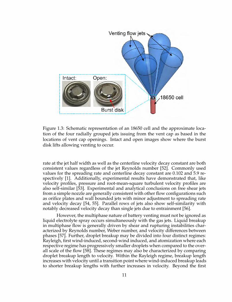
Figure 1.3: Schematic representation of an 18650 cell and the approximate loca-tion of the four radially grouped jets issuing from the vent cap as based in thelocations of vent cap openings. Intact and open images show where the burstdisk lifts allowing venting to occur.

rate at the jet half width as well as the centerline velocity decay constant are bothconsistent values regardless of the jet Reynolds number [52]. Commonly usedvalues for the spreading rate and centerline decay constant are 0.102 and 5.9 re-spectively [1]. Additionally, experimental results have demonstrated that, likevelocity profiles, pressure and root-mean-square turbulent velocity profiles arealso self-similar [53]. Experimental and analytical conclusions on free shear jetsfrom a simple nozzle are generally consistent with other flow configurations suchas orifice plates and wall bounded jets with minor adjustment to spreading rateand velocity decay [54, 55]. Parallel rows of jets also show self-similarity withnotably decreased velocity decay than single jets due to entrainment [56].

However, the multiphase nature of battery venting must not be ignored asliquid electrolyte spray occurs simultaneously with the gas jets. Liquid breakupin multiphase flow is generally driven by shear and rupturing instabilities char-acterized by Reynolds number, Weber number, and velocity differences betweenphases [57]. Further, droplet breakup may be divided into four distinct regimes:Rayleigh, first wind-induced, second-wind induced, and atomization where eachrespective regime has progressively smaller droplets when compared to the over-all scale of the flow [58]. These regimes may also be characterized by comparingdroplet breakup length to velocity. Within the Rayleigh regime, breakup lengthincreases with velocity until a transition point where wind-induced breakup leadsto shorter breakup lengths with further increases in velocity. Beyond the first

11

wind-induced regime, the second wind-induced regime shows breakup down-stream or the orifice while atomization occurs at the orifice itself [59].

In the case of battery failures, previous work has visualized the high ve-locity flow resulting in droplet atomization [45], and the bulk geometry of such aspray is of importance. Within the atomization regime, spray angle is a functionof fluid densities, nozzle or orifice geometry, and Taylor parameter which itselfis a function of Reynolds and Weber numbers [60]. The geometric parameter fordetermining the spray angle shows some trends within similar designs, but gen-erally is determined for each unique nozzle or orifice design [61]. The spray angleis not greatly affected by the gas momentum within the flow [62]. The velocityprofile of droplets within a spray follows similar trends to that of a free shear jet,but increases in the droplet Stokes number have been demonstrated to increasethe potential core velocity profile and significantly delay spreading [63].

Combustible spray systems pose additional challenges and parameters tobe characterized. Characterization of relative performance between combustablesprays often relies on experimental characterization of spray tip penetration (STP),Sauter Mean Diameter (SMD), and mean velocity distributions [64]. High-speedschlieren imaging with digital image post-processing have effectively visualizeddroplet spray characteristics including STP, cone angle, and projected area [65].

Experimental measurement of the particle and velocity fields can be per-formed using various techniques, but PIV has become nearly an industry stan-dard. This experimental method provides full field velocity measurements bycorrelating groups of particles between time-resolved image pairs and quantify-ing their displacement within the field of view [66]. Stokes number is used todescribe whether a particle closely follows the surrounding flow and is definedas the ratio of the relaxation time of the particle to a characteristic timescale of theflow. In PIV applications, a Stokes number much smaller than unity is desired.Using the Stokes flow approximation, the relaxation time of the particle is a func-tion of diameter, particle density, and surrounding fluid viscosity [67]. Depend-ing on the flow conditions, illumination hardware, and camera specifications,various solid or liquid particles with different sizes and densities may be chosenfor different PIV applications. Experimental work has determined the accuracyof tracing in terms of maximum relative slip velocity between the particle andflow as a function of Stokes number [68]. In general, it is desirable to have trac-ing particle diameters on the order of 1 µm in turbulent and high speed flows, butporous or hollow particles with low density may also be used [69]. Oil dropletson this diameter scale have been successfully used for PIV measurement of thevelocity profile of Mach 1.5 impinging jets within 1% of the velocity predicted byisentropic flow relations [70]. Other applications with high speed flows measuredby PIV include flow over wings in supersonic wind tunnels and shock boundarylayer interactions [71, 72]. The related technique of Particle Tracking Velocimetry(PTV) technique can be used in a similar way to PIV with more sparse particleseeding by tracking individual particles [73]. While seeding particles may beadded to follow a transparent, gaseous flow, PIV can also be used to visualizedroplets within a spray. In this way, PIV techniques are especially well suited for

12

characterization of lithium ion battery venting.

1.4 Present research objectives

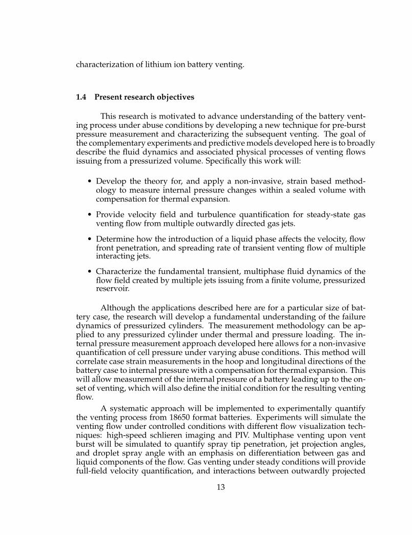
This research is motivated to advance understanding of the battery vent-ing process under abuse conditions by developing a new technique for pre-burstpressure measurement and characterizing the subsequent venting. The goal ofthe complementary experiments and predictive models developed here is to broadlydescribe the fluid dynamics and associated physical processes of venting flowsissuing from a pressurized volume. Specifically this work will:

• Develop the theory for, and apply a non-invasive, strain based method-ology to measure internal pressure changes within a sealed volume withcompensation for thermal expansion.

• Provide velocity field and turbulence quantification for steady-state gasventing flow from multiple outwardly directed gas jets.

• Determine how the introduction of a liquid phase affects the velocity, flowfront penetration, and spreading rate of transient venting flow of multipleinteracting jets.

• Characterize the fundamental transient, multiphase fluid dynamics of theflow field created by multiple jets issuing from a finite volume, pressurizedreservoir.

Although the applications described here are for a particular size of bat-tery case, the research will develop a fundamental understanding of the failuredynamics of pressurized cylinders. The measurement methodology can be ap-plied to any pressurized cylinder under thermal and pressure loading. The in-ternal pressure measurement approach developed here allows for a non-invasivequantification of cell pressure under varying abuse conditions. This method willcorrelate case strain measurements in the hoop and longitudinal directions of thebattery case to internal pressure with a compensation for thermal expansion. Thiswill allow measurement of the internal pressure of a battery leading up to the on-set of venting, which will also define the initial condition for the resulting ventingflow.

A systematic approach will be implemented to experimentally quantifythe venting process from 18650 format batteries. Experiments will simulate theventing flow under controlled conditions with different flow visualization tech-niques: high-speed schlieren imaging and PIV. Multiphase venting upon ventburst will be simulated to quantify spray tip penetration, jet projection angles,and droplet spray angle with an emphasis on differentiation between gas andliquid components of the flow. Gas venting under steady conditions will providefull-field velocity quantification, and interactions between outwardly projected

13

jets will be described in terms of parameterized spreading rates and velocity de-cay constants. Additional analysis of steady state venting will include turbulencestatistics and description of jet interactions in the velocity fields. The fluid dy-namic investigations here ultimately develop a fundamental understanding ofhow multiple transient turbulent jets interact and how multiphase flow alters thejet behavior and transient development.

Optical flow measurements provide a more thorough characterization ofthe fluid dynamics of a battery failure than previously attained. Primarily, agreater scientific knowledge of lithium ion battery safety will be developed asthe physical mechanism contributing to their greatest hazards will be uniquelyunderstood.

14

CHAPTER 2

THEORY AND VALIDATION OF STRAIN-BASED INTERNALPRESSURE MEASUREMENT

Under abuse conditions, batteries exhibit a contained build up of pressureuntil the moment of vent mechanism burst. Pressure build up is the result of thethermal runaway process. The ability to measure this pressure rise is importantto understand the onset of venting and the processes that lead up to it. Tightlywound, delicate electrochemical components within the cell make accessing theinside of the battery case for direct pressure measurement virtually impossiblewithout damaging the battery or affecting how it responds to abuse. Here, mea-surement of the cylindrical case’s mechanical response to the build up of internalpressure avoids these limitations. Experiments were performed to demonstratehow strain gauges may used to perform noninvasive pressure measurement ofbatteries under thermal abuse conditions. Further, this experimental methodol-ogy may be applied to any pressurized cylinder.

2.1 Theoretical basis of experiment

Pressure contained within an enclosed cylinder will cause mechanical stressalong its length and around its circumference in what are referred to as longitu-dinal and hoop components, respectively. To measure these stress components,two strain gauges are adhesively bonded to the outside of the cylinder wall. Eachstrain gauge has a resistive grid which is oriented in the direction of the stresscomponent it measures as shown in Figure 2.1.

2.1.1 Thin walled method

Typical 18650 battery cases have a wall thickness that is much smaller thantheir diameter. Analysis of thin walled cylinders treats stress within a small finiteregion of the outer case of a cylindrical, pressurized vessel as two dimensionaland planar with stress components around the circumference (hoop) and alongthe length (longitudinal) of the cylinder. For a thin walled cylinder, analytic ex-pressions relate hoop (σH) and longitudinal (σL) stress to the internal pressure (P)within the cell as described by:

15

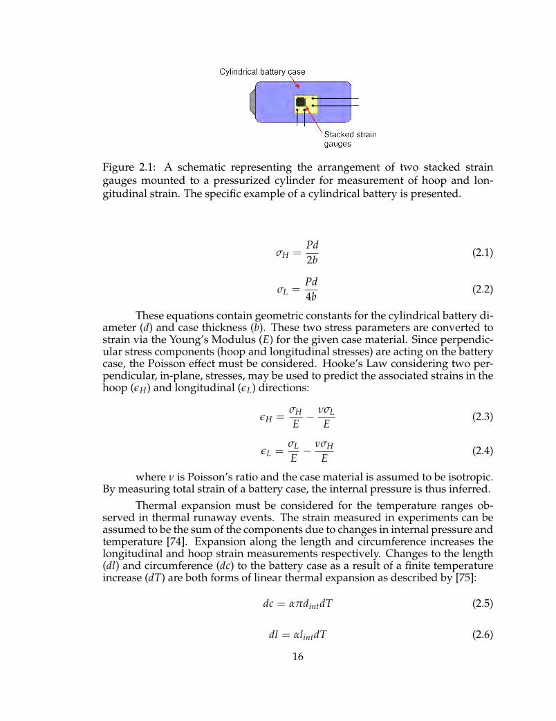
Figure 2.1: A schematic representing the arrangement of two stacked straingauges mounted to a pressurized cylinder for measurement of hoop and lon-gitudinal strain. The specific example of a cylindrical battery is presented.

σH =Pd2b

(2.1)

σL =Pd4b

(2.2)

These equations contain geometric constants for the cylindrical battery di-ameter (d) and case thickness (b). These two stress parameters are converted tostrain via the Young’s Modulus (E) for the given case material. Since perpendic-ular stress components (hoop and longitudinal stresses) are acting on the batterycase, the Poisson effect must be considered. Hooke’s Law considering two per-pendicular, in-plane, stresses, may be used to predict the associated strains in thehoop (εH) and longitudinal (εL) directions:

εH =σH

E− νσL

E(2.3)

εL =σL

E− νσH

E(2.4)

where ν is Poisson’s ratio and the case material is assumed to be isotropic.By measuring total strain of a battery case, the internal pressure is thus inferred.

Thermal expansion must be considered for the temperature ranges ob-served in thermal runaway events. The strain measured in experiments can beassumed to be the sum of the components due to changes in internal pressure andtemperature [74]. Expansion along the length and circumference increases thelongitudinal and hoop strain measurements respectively. Changes to the length(dl) and circumference (dc) to the battery case as a result of a finite temperatureincrease (dT) are both forms of linear thermal expansion as described by [75]:

dc = απdintdT (2.5)

dl = αlintdT (2.6)

16

The subscript int denotes the initial battery length and diameter. The co-efficient of thermal expansion (α) is a material property and assumed constantover the temperature changes expected. By noting that engineering strain (ε)is defined as the change in length to the original length of an object, Equations2.5 and 2.6 may be rearranged to show that the component of case strain due tochanges in temperature may be expressed as the product of the thermal expan-sion coefficient and the finite temperature change.

Summing the components of strain due to internal pressure and tempera-ture increases gives [76]:

εH =σH

E− νσL

E+ αdT (2.7)

εL =σL

E− νσH

E+ αdT (2.8)

Equations 2.7 and 2.8 represent the measurements that would be recordedby strain gauges mounted to a battery in the hoop and longitudinal directions asit undergoes thermal abuse. These two equations may be subtracted from oneanother to eliminate the effects of thermal expansion giving:

εH − εL =1 + ν

E(σH − σL) (2.9)

Substituting the expressions for hoop and longitudinal stress from Equa-tions 2.1 and 2.2 gives:

εH − εL =1 + ν

E

(Pd2b− Pd

4b

)(2.10)

Solving the above equation for internal pressure gives:

P =4Eb

d(1 + ν)(εH − εL) (2.11)

This expression states that the internal pressure is proportional to the dif-ference of the two strain measurements.

2.1.2 Thick wall method

As the assumption of a thin cylindrical shell becomes less applicable aswall thickness increases, additional analytical expressions exist for a thick wallscenario [77]. In particular, the hoop (subscript H, t) and longitudinal (subscriptL, t) stress relationships for a thick wall on the outer surface are:

17

σH,t =2Pr2

ir2

o − r2i

(2.12)

σL,t =Pr2

ir2

o − r2i

(2.13)

where ro and ri are the outer and inner cylinder radii respectively. For clar-ity the geometric relationships d = 2ro and b = ro − ri hold true, but expressingthick wall hoop and longitudinal stress in terms of diameter (d) and case thick-ness (b) in a manner similar to the thin wall equations is cumbersome.

Noting that the relationship in Equation 2.9 is determined from plane stressand linear thermal expansion relationships and not the thin wall method itself, asimilar equation can be written by replacing σH and σL with σH,t and σL,t respec-tively:

εH,t − εL,t =1 + ν

E(σH,t − σL,t) (2.14)

Substituting Equations 2.12 and 2.13 into Equation 2.14 gives:

εH,t − εL,t =1 + ν

E

(2Pr2

ir2

o − r2i−

Pr2i

r2o − r2

i

)(2.15)

which may be solved for a pressure relationship similar to Equation 2.11for the thick wall method as:

Pt =E

1 + ν

(r2

o − r2i

r2i

)(εH,t − εL,t) (2.16)

where pressure (Pt for thick wall method) is again proportional to the dif-ference in the strain measurements, but the coefficient has changed from the thinwall method.

2.1.3 Comparison of the thin and thick wall methods

It can be noted from Equations 2.1, 2.2, 2.12, and 2.13, that hoop stressis always twice the longitudinal stress within both analytical models. The onlydifference between the relationships is how the parameters related to cylindergeometry are treated. The cylinder geometry in the thin wall case affects straincomponents via the parameter:

18

db

(2.17)

whereas the geometry affects thick wall case stress via:

r2i

r2o − r2

i(2.18)

Through substitution of the geometric relationships between radius (innerand outer), diameter, and thickness, it can be shown that:

r2i

r2o − r2

i=

db

(d2/4− db + b2

d2 − db

)(2.19)

Since the term within the parenthesis in Equation 2.19 defines the rela-tionship between thin and thick wall stress relationships, this parameter may becalled a relative shape factor and given the symbol δ. Accordingly:

r2i

r2o − r2

i=

db(δ) (2.20)

with:

δ =d2/4− db + b2

d2 − db(2.21)

Using this relative shape factor, the hoop and longitudinal stress relation-ships for the thick wall method can be rewritten in terms of their respective com-ponents from the thin wall method as (by letting P = Pt):

σH,t = 2P(

db

δ

)= 4δ

Pd2b

= 4δσH (2.22)

σL,t = P(

db

δ

)= 4δ

Pd4b

= 4δσL (2.23)

In both of the above equations, the ratio of corresponding stress compo-nents from the two analysis methods is consistently 4δ. Symbolically:

σH,t

σH=

σL,t

σL= 4δ (2.24)

Examining the shape factor δ at a case thickness of zero:

19

Figure 2.2: The ratio of respective stress components calculated via thick and thinwall methods as a function of the ratio of case thickness to outer diameter.

d2/4− d(0) + (0)2

d2 − d(0)=

14

(2.25)

demonstrates that Equations 2.22 and 2.23 reduce to σH,t = σH and σL,t =σL respectively. Thus, the thick and thin wall stress methods are equivalent whencase thickness is zero. As the case thickness increases towards b/d = 0.5, asolid cylinder, the ratio between thick method stress and thin method stress ap-proaches zero as shown in Figure 2.2

For completeness, the ratio of internal pressures calculated from Equations2.11 and 2.16 yields:

Pthin method

Pthick method=

PPt

= 4δ (2.26)

The thin wall method will thus underrepresent the internal pressure con-tained within a cylinder as the thickness increases. In most scenarios, including18650 format batteries, the thin wall stress method is acceptable and results ina discrepancy of approximately 2%. Selection of thin versus thick method forindividual tests is discussed further in Section 2.7.

2.1.4 Considerations and anticipated limitations

Values for cell diameter, case thickness, Poisson’s Ratio, and Young’s Mod-ulus can be measured directly with material testing. However, these parameters

20

may be estimated if experimental strain data can be fixed to a known pressurestate of the cell. This could be the battery state at the moment of venting onsetwhere strain is expected to reach a maximum value which can be related to theexpected burst pressure as reported in the literature [78]. Variability in this esti-mation between pressure and strain states would be influenced by the results ofdirect vent pressurization testing.

Limitations of this approach include localized failures within the cell. Thiscould include deformations of interior battery components associated with eventssuch as an internal short. Gas generation can also be localized within the cell priorto failure (e.g. trapped between anode and cathode layers), leading to nonuni-form pressure distribution. To address this, initial tests were performed withmultiple sets of strain gauges on a single cell.

Variable case thickness or other geometric irregularities leading to strainconcentrations will have an effect on the accuracy of Equation 2.11. Hoop andlongitudinal strain relations are derived for an even internal pressure. Thus, in-consistent internal pressure or the presence of other force loading on the cylin-drical shell will decrease the accuracy of pressure calculations. To address this,initial tests will be performed with multiple sets of strain gauges on a single cell.

2.2 Expected strain measurement range

Using Equation 2.11 for internal pressure and Equations 2.7 and 2.8 forstrain, approximations can be made to identify the range of strain measurementsanticipated. This informed data acquisition techniques and equipment used. Pre-vious work determined that 18650 format cells generally begin venting before aninternal pressure of 3 MPa and temperature of 200 °C [9, 47, 13]. Battery cases areoften constructed from tool steels such as A3 which has properties listed in Table2.1 [16, 79, 80]. Typical empty battery cases sold as components have diametersof 18 mm with a thickness of 0.25 mm.

Table 2.1: Approximate tool steel properties used in battery case constructionProperty Symbol Value

Young’s Modulus E 200 GPaPoisson’s Ratio ν 0.285

Thermal expansion coefficient α 10.7 · 10−6 1/°C

From Equation 2.9, hoop strain must always be larger than longitudinalstrain. By substituting a pressure of 3 MPa and temperature of 200 °C into Equa-tion 2.7, the maximum reasonable hoop strain measurement is 2,600 µε. At thissame temperature and pressure, Equation 2.8 provides a maximum reasonablelongitudinal strain measurement of 2,260 µε. For both of these strain measure-ments the portion of strain due to thermal loading is 2,140 µε.

21

For clarity, microstrain (µε) is used here to specify engineering strain (ε)without repeatedly noting multiplication by 10−6. Engineering strain in the lon-gitudinal direction (εL) is:

εL =∆llint

(2.27)

where ∆l is elongation due to internal pressure build up and lint originallength. Similarly in the hoop direction, engineering strain is:

εH =∆ccint

=∆ddint

(2.28)

where cint original circumference and ∆c is the change in circumferenceafter internal pressure has increased. Hoop strain is thought of as a change incircumference for consistency with the planar stress assumptions of the thin wallmethod, but hoop strain may also be considered in terms of original diameter(dint) and diameter change (∆d).

2.3 Strain measurement corrections

While ideal strain gauges and experimental conditions would provide straindata which are immediately able to be used for internal pressure measurement,real limitations exist regarding thermal output, substrate curvature, transversesensitivity, and gauge misalignment. To fully correct for these errors, the rawdata is initially corrected for thermal output and the incremental thermal outputassociated with substrate curvature which occurs in the hoop direction. Thesetwo thermal outputs are mainly related to relative thermal expansion betweenthe gauge and test specimen. This step is done initially because these errors area function of the gauge and test specimen combination and are not affected bythe experimental stress state. The second correction for transverse sensitivity re-moves any numerical dependence between the hoop and longitudinal strain val-ues. Last, gauge misalignment is accounted for via a simple coordinate rotation.

Thermal output is caused by a relative thermal expansion mismatch be-tween the strain gauge and the substrate along with electrical material propertychanges at elevated temperatures. While care was taken in selection of straingauges to match the steel substrates used throughout testing, this factor cannotbe eliminated entirely at the temperatures associated with battery abuse testing.As such, a thermal output correction function was used as provided by the man-ufacturer in the form: [81]

εT/O = A0 + A1T + A2T2 + A3T3 + A4T4 + A5T5 (2.29)

22

where A0 through A5 are constants provided with each gauge design andT is the temperature in degrees Celsius. For the strain gauges used in these ex-periments, the thermal output correction coefficients are listed in Table 2.2.

Table 2.2: Thermal output coefficients for Vishay WK-06-120WT-350 straingauges

Coefficient ValueA0 −4.63× 101 µεA1 2.38× 100 µε/°CA2 −1.80× 10−2 µε/°C2

A3 2.84× 10−5 µε/°C3

A4 1.15× 10−7 µε/°C4

A5 −3.70× 10−10 µε/°C5

The thermal output (εT/O) is given as a strain to be subtracted from themeasured strain such that:

εthermal corrected = εmeasured − εT/O (2.30)

In the hoop direction specifically, the cylindrical substrate is sufficientlycurved such that an additional thermal output correction is needed. This incre-mental thermal output (∆εT/O) is calculated from the equation:

∆εT/O =1R[(1 + 2νA−B) (hAαA + hBαB)− 2νA−BαS (hA + hB)]∆T (2.31)

where R is the radius of curvature of the substrate (here the radius of cur-vature of the battery case is used), νA−B is the average Poisson’s ratio of the ad-hesive and backing, hA is adhesive thickness, hB is gauge backing thickness, αAis the thermal expansion coefficient of the adhesive, αB is the thermal expansioncoefficient of the gauge backing, αS is the thermal expansion coefficient of thesubstrate, and ∆T is the change in temperature from reference temperature [82].All of these coefficients are provided by the strain gauge manufacturer [81].

In the configuration of interest here with perpendicular measurements ofhoop and longitudinal strain, the thermal output corrected values are correctedfor transverse sensitivity via Equations 2.32 and 2.33 [83]. Transverse sensitiv-ity arises because foil grid style gauges (as used here) change resistance whenstrained in any direction. While the grid is designed to maximize sensitivity inthe desired measurement axis, the electrical connections at the ends of these runsdisplay small resistive changes under strain in the perpendicular direction. Ofnote, ν0 is the substrate’s Poisson’s ratio, and Kt is the manufacturer providedtransverse sensitivity factor.

23

εH, transverse, thermal corrected =(1− ν0Kt) (εH, thermal corrected − KtεL, thermal corrected)

1− K2t

(2.32)

εL, transverse, thermal corrected =(1− ν0Kt) (εL, thermal corrected − KtεH, thermal corrected)

1− K2t

(2.33)The last correction performed is an in-plane rotation through angle θ to

correct for any misalignment of the gauges which may occur during the bondingor adhesive curing phases of gauge mounting. The angle φ is measured afterthe gauge mounting process where the rotation is observed as a misalignmentbetween alignment markings on the strain gauge and a burnished layout linealong the length of the test specimen. The equations below are used to arrive atfinal corrected strain values from the transverse/thermal corrected strains:

εH, final = εH, transverse, thermal corrected cos2 φ

+ εL, transverse, thermal corrected sin2 φ + 2τHL sin θ cos φ(2.34)

εL, final = εL, transverse, thermal corrected cos2 φ

+ εH, transverse, thermal corrected sin2 φ + 2τHL sin φ cos φ(2.35)

where the shear term τHL is given by:

τHL =12

tan (2φ) (εH, transverse/thermal corrected − εL, transverse/thermal corrected) (2.36)

2.4 Design of laboratory test setup

A test facility was designed and constructed to measure the external casestrain of 18650 format batteries under thermal abuse conditions. The test setupconsists of a heated cylindrical chamber with ports for instrumentation and aviewing window shown in Figure 2.3(a). A 4-NPT-size, Schedule 160, steel pipesection is used to create the body of the chamber, and standard pipe flanges arethreaded to the ends to provide rigid mounting points for removable end caps.The chamber interior space is 87 mm in diameter by 305 mm long. End caps incor-porate instrumentation pass-throughs on one side of the chamber and a battery

24

Figure 2.3: Images of the test setup installed at New Mexico Tech including (a)the test chamber, (b) instrumentation end cap, (c) insulation structure, and (d)battery holder.

viewing window on the other. Figure 2.3(b) shows the completed instrumen-tation end cap which has ports for a thermocouple probe to measure chambergas temperature, three reconfigurable passthroughs for thermocouples and straingauge leads, and an inlet and outlet for a remote purge system. Thermocouplesare embedded into the main body of the test chamber to measure the temperaturegradient within the steel, thus allowing calculation of heat flux into the chamber.

The chamber body is evenly wrapped with three electrical rope heaters(Hotwatt brand, model: GR30-120/960w120v/sf1-6) each capable of outputting960 W (2,880 W total) to create even heating within the chamber interior. Achiev-ing high heating rates in the chamber is important to be able to subject batteries todifferent abuse scenarios. A flexible insulation wrap made of fiberglass, ceramicfiber, and Nomex is placed around the test chamber body immediately outside ofthe rope heaters and secured with stainless steel pipe clamps. The test chamberitself is placed inside of a rigid insulation structure shown in Figure 2.3(c). Thisstructure is fabricated from laser cut acrylic sheeting and has a modular designof double-pane panels. A final step taken in improving heat transfer to batteries

25

is the use of a helium environment inside the chamber. This improves heat trans-fer significantly as helium has a high thermal conductivity value of 0.142 W/mKcompared to a value of 0.024 W/mK for air.

During an initial heating test there was an unpredicted cascading failureof the rope heaters at a chamber temperature of 275 °C. All subsequent tests werelimited to a maximum chamber temperature of 225 °C while the heaters were onto provide a safety margin for the resiliency of the test apparatus.

A battery holder was designed and fabricated to securely hold a cell priorto and during venting within the center of the test chamber. Shown in Figure2.3(d), the holder uses laser cut, high temperature silicone rubber cradles with aseries of aluminum rings and standoffs. This holder fits within the inner diame-ter of the test chamber with minimal movement. The cradle shape of the siliconeis designed to allow the battery to expand freely throughout testing and to notcause any stress concentrations which would negatively affect strain measure-ments. Two small silicone rubber rings are laser cut and placed on one side of thebattery case adjacent to the two sides of a silicone holder to minimize movementduring positioning. The strain these rings places near the end of the battery caseare negligible.

Data acquisition is performed with a National Instruments (NI) cDAQ sys-tem and controlled through LabVIEW. The system is configured to record tem-perature, strain, and pressure data as well as control the operation of inlet andexit valves used for remote purge of the gas within the chamber after a test. FourJ-type thermocouples are embedded in pairs on opposite sides of the chamberwall. Each pair has a thermocouple at a depth of 3.3 mm and 10.1 mm whichcorrespond to roughly 25% and 75% of the wall thickness, respectively. K-typethermocouples are used to measure interior chamber gas temperature and surfacetemperature of the battery on the side of the case and on the positive terminal atthe end of the vent cap. Chamber static pressure is also recorded and monitoredthroughout testing.

Micro-Measurements brand perpendicularly oriented, stacked strain gauges,shown in Figure 2.4, are bonded to the outer surface of the test specimens with ahigh temperature, two part epoxy which cures at room temperature (HBM brand,X280 adhesive). Mounted at 90° to each other, the stacked gauge configurationallows mounting over a single location on the cylinder. These gauges have anominal gauge factor (GF) of 2.02. Each strain gauge is wired in a three-wire,quarter bridge configuration with 350 Ω resistors using RJ50 style circuit comple-tion breakouts from a NI 9237 strain gauge measurement card. The quarter bridgearrangement provides adequate thermal compensation as hoop and longitudinalstrain values are to be subtracted from each other as previously discussed. Thismeasurement card has an input range of ±25 mV/V in terms of the ratio of mea-surement voltage to excitation voltage with a 24-bit resolution. This correspondsto a measurement precision of 3.0 · 10−6 mV/V. To complete the quarter bridgewiring configuration, solder pads are bonded to the test specimen surface simi-larly to the strain gauge. These solder pads provide a secure electrical connectionand strain relief to prevent damage to gauges while being installed into the test

26

chamber.

Figure 2.4: Micro-Measurements brand, model WK-06-120WT-350 strain gauges.Two strain gauges are incorporated into a single unit and are arranged at rightangles to allow simultaneous measurement in the hoop and longitudinal direc-tions.

The ratio of measurement voltage (VOUTPUT) to excitation voltage (VEX)for a quarter bridge configuration is [84]:

VOUTPUT

VEX= −GF · ε

4

(1

1 + GF · ε2

)(2.37)

With the previously calculated maximum anticipated strain values of 2,600 µεin the hoop direction and 2,260 µε in the longitudinal direction, the largest volt-age ratio measurements will be -1.31 mV/V and -1.14 mV/V respectively. Bysubstituting the precision of the voltage ratio measurement into Equation 2.37,the strain measurement precision is 5.9 · 10−3 µε.

2.5 Heating rate calibration series

A necessary step in the validation of the test setup was calibrating thesystem to have predictable interior heating rates as a function of the electricalpower output of the heaters. Calibration tests were performed on the test cham-ber at electrical power values ranging from 576 W to 2,308 W by varying the in-put voltage to the electrical heaters with a variable autotransformer. Three tests

27

were conducted at power settings corresponding to 20%, 50%, and 80%. Each testheated the chamber for 60 min or until a chamber gas temperature measurementof 225 °C was reached. All tests started with zero gauge pressure and the chamberat room temperature. Temperature and pressure data were recorded throughout.Interior gas temperature increases and associated linear fits for this calibrationtesting are shown in Figure 2.5(a). Temperature increases were approximated aslinear to provide a nominal heating rate useful in comparison to other calorime-try testing. Linear fits are calculated as regressions of chamber temperature froma time of 5 min to the end of the test. The nominal heating rates for the calibrationtests follow a linear relationship with the heater setting as shown in Figure 2.5(b).Extrapolation of the data yields a maximum possible rate of 9.57 °C/min at themaximum heater setting of 2,880 W. However, tests were kept below this rate tominimize the risk of heater failures.

Figure 2.5: (a) Gas temperature increase versus time and linear fits for the heat-ing rate calibration test series, and (b) plotting the nominal heating rate versuselectrical power input for these tests.

2.6 Uncertainty estimation for strain based pressure measurement

Uncertainty propagation calculations were performed on the final internalpressure measurement equations developed for thin and thick wall cylinders toaccount for uncertainty in strain measurements, geometry, and material proper-ties. Uncertainty for the thin and thick wall internal pressure measurements wererespectively calculated as [85]:

28

∆P =

((∂P∂E

∆E)2

+

(∂P∂ν

∆ν

)2

+

(∂P∂b

∆b)2

+

(∂P∂d

∆d)2

+

(∂P

∂εH∆εH

)2

+

(∂P∂εL

∆εL

)2)1/2 (2.38)

and

∆Pt =

((∂Pt

∂E∆E)2

+

(∂Pt

∂ν∆ν

)2

+

(∂Pt

∂b∆b)2

+

(∂Pt

∂d∆d)2

+

(∂Pt

∂εH∆εH

)2

+

(∂Pt

∂εL∆εL

)2)1/2 (2.39)

where the partial differential terms are easily calculated from Equations2.11 and 2.16. Since both strain measurements varied throughout each experi-ment, many of the partial differential terms varied accordingly, and uncertaintywas calculated continuously throughout each experiment. In general, as strainmeasurements increased throughout experiments exhibiting a pressure build up,the uncertainty also increased.

Individual parameter uncertainty values in Equations 2.38 and 2.39 wereapproximated for each of the parameters used to calculate internal pressure un-certainty (∆P or ∆Pt). Uncertainty in case thickness (b), diameter (d), outer radius(ro), and inner radius (ri) are all approximated to be equivalent to the 0.01 mm de-gree of measurement of the digital calipers used to perform these measurements.Strain measurement uncertainty in both directions was calculated as 2.8 µε. Thisvalue corresponds to twice the standard deviation of strain measurement noisebands recorded on static, unheated test samples. Material properties were not ex-pected to vary significantly between similar samples in both validation and livecell tests, and were estimated at 5% for incorporation in uncertainty propagation.These uncertainty calculations were used to apply error bars on internal pressuremeasurement traces for both validation experiments and live battery abuse testsas reported in Figures 2.9, 2.12, and 3.8.

While material properties including Young’s Modulus and Poisson’s Ratiowere not expected to vary significantly between similar samples, these proper-ties demonstrated the largest potential source of systematic error in the measure-ments which is attributed to a lack of precise manufacturer specified properties.Thin steel specimens of various grades demonstrated variances of up to approx-imately 20% from typical, approximately 200 GPa Young’s Modulus values [86].Similarly, Poissons Ratio is approximated to vary up to 0.015 (unitless) [87]. These

29

variances from typical values were not included in this uncertainty approxima-tion because they represented a systematic error causing a change in the slopeof entire pressure trends rather than a continually varying, random uncertaintyassociated with the recorded measurements.

2.7 Validation experiments

2.7.1 Measurement of thermal response from 18650 battery case

Two validation experiments were conducted to demonstrate the strain basedinternal pressure measurement approach. The first experiment involved heatingan empty 18650 battery case to demonstrate the thermal expansion componentwithin the strain measurements. The empty 18650 battery case was purchased asan unassembled cell component and was simply a thin-walled cylinder with oneend closed and the other end open. There were no electrochemical componentsinstalled, and there was no vent cap crimped into place. Since the cylinder wasopen, no pressure built up. As such, hoop and longitudinal strain measurementsas described in Equations 2.7 and 2.8 reduce to the thermal expansion term. Thehoop and longitudinal strain measurements were thus expected to be identical inthis scenario.

The thermal expansion validation was performed at a heater power of 50%which corresponds to a nominal heating rate of 4.8°C/min until a maximum sur-face temperature of 180°C was observed. The trial was run in duplicate to addressrepeatability. Shown in Figure 2.6, the strain gauge was mounted to the center ofthe battery case, and no de-lamination was noted during or after testing. Slightdarkening of the epoxy adhesive and a hazing of the PEEK plastic insulation onthe strain gauge lead wires were noted, but were not correlated to any lack inmeasurement performance.

Shown in Figures 2.7 and 2.8 hoop and longitudinal strain were mea-sured throughout the heating process. The dashed lines represent the raw dataas recorded in LabVIEW while the solid lines have been corrected for thermal,curvature, transverse sensitivity, and misalignment effects as described in Sec-tion 2.3. In both trials, the corrected values report strain values closer to zerothan the raw data. While thermal output correction attempts to remove mosterroneous measurement, strain typically increases with some notable non-lineartrends throughout the heating of the battery case. Strain values in both trials, inhoop and longitudinal directions, show an initial linear increase in strain as tem-perature increases prior to a broad peak between 60°C and 100°C followed bysubsequent fluctuations. Since hoop and longitudinal strain measurements fol-low somewhat similar, even if highly non-linear, trends, pressure measurementsretain a degree of confidence because it is calculated from the more consistentdifference between the two measured values.

30

Figure 2.6: Open 18650 size battery case with strain gauge and data acquisitionwiring attached.

Both trials show trends on the same order of magnitude, but the measuredthermal effects were greatest in the first trial (Figure 2.7). This is attributed to un-known residual stresses within the battery case which were a result of the cold-worked fabrication method of the steel. As metal was heated, there may havebeen some internal stress relief in the battery case which resulted in lower effectsobserved in the second thermal expansion trial which was performed with thesame case. Another uncertainty which was systematically minimized in subse-quent tests was the screw connections between the soldered in place strain gaugewires and the permanent data acquisition wires. Since these wires are connectedvia a screw connection, the compression of the crimped wire ferrules on the straingauge leads may have a slightly variable contact resistance. This is further com-pounded with the compression of the ferrules potentially changing as differentialthermal expansion may have occurred between dissimilar metals in the electricaljunctions. In the second trial, the screw connections were tightened until the fer-rules completely crushed and the screws were unable to be tightened further.This should provide more consistent contact resistance between tests.

The raw and corrected strain measurements from Figures 2.7 and 2.8 wereused to calculate an indicated pressure in both open case trials. As shown inFigure 2.9, the data show a nonzero internal pressure. Since the case is open,this indicated pressure is clearly nonphysical and is presented to demonstratean upper bound of the measurement uncertainty. Corrected strain values fromboth trials demonstrate a range of pressure uncertainty of approximately 400 kPawhere the indicated pressure increases during the first trial and fluctuated aroundzero for the second. The open 18650 battery case trials demonstrate the ability toimprove measurement uncertainty via the corrections described in Section 2.3,and provide a means to bound the certainty of measurements taken in live celltests.

31

Figure 2.7: Raw and corrected strain measurement values versus temperature forthe first open battery case thermal expansion validation trial

2.7.2 Internal pressure rise from constant volume heating of a carbondioxide cartridge

A second more rigorous demonstration of the system capabilities was per-formed in which a carbon dioxide cartridge was heated until failure. These car-tridges are small, pressurized cylinders containing nominally 12 g of carbon diox-ide common in bicycle tire inflators and compressed gas pellet guns. The de-formation of these cartridges is governed by the same hoop and longitudinalstress relations as a cylindrical battery. Under increased temperature, the pres-sure within the cartridge must increase predictably according to the Ideal GasLaw as plotted in Figure 2.10. The pressure increase as a function of temper-ature is calculated here as a constant volume heating from the National Insti-tute of Standards and Technology (NIST) REFPROP database [88]. Throughoutthis process, the contained volume of carbon dioxide is at a constant density, be-cause there is a fixed mass at fixed volume, which must be known to define thepressure-temperature curve.

In addition to the internal pressure measurement technique validation,this experiment is designed demonstrate the containment capability of the calorime-ter fixture and cradle, as the carbon dioxide cartridge is likely to fail and vent attemperatures lower than the venting onset point for many 18650 format batteries.

Density within a Crossman brand carbon dioxide cartridge was calculatedto an average value of 840 kg/m3. This was calculated by measuring the volumeof the cartridges via water displacement then measuring mass before and after

32

Figure 2.8: Raw and corrected strain measurement values versus temperature forthe second open battery case thermal expansion validation trial

piercing the case and venting the carbon dioxide. Using a density of 7,860 kg/m3,the volume of the steel case was calculated. The volume difference between thetotal cartridge and the steel case is the carbon dioxide volume, and the differencein the two mass measurements is the amount of carbon dioxide originally con-tained within the cartridge. Five samples were tested and are reported in Table2.3.

Table 2.3: Volume (V) and mass (m) measurements of Crossman brand carbondioxide cartridges to calculate carbon dioxide density (ρ)

Sample Cartridge Cartridge Steel case Steel case CO2 CO2 CO2V (mL) m (g) V (mL) m (g) V (mL) m (g) ρ (kg/m3)

1 19.0 43.71 3.90 30.69 15.1 13.02 8632 19.5 43.47 3.91 30.72 15.6 12.75 8183 19.0 42.79 3.84 30.21 15.2 12.58 8304 19.0 43.65 3.92 30.83 15.1 12.82 8505 19.0 43.20 3.88 30.53 15.1 12.67 838

Mean 19.1 43.36 3.89 30.59 15.2 12.77 840

After determining the carbon dioxide density contained within one of thecartridges, strain gauges were bonded to four samples from the same productionbatch as shown in Figure 2.11(a). Three of the sample cartridges were tested aspurchased while another was pierced at the reduced diameter end to relieve pres-

33

Figure 2.9: Indicated pressure as a function of temperature for the open case val-idation trials

sure and create an unpressurized baseline reference. Each cartridge was heateduntil failure or a surface temperature of 180°C at a rate of 4.8°C/min. Failure ofthe pressurized cartridges occurred at temperatures between 80°C and 100°C forall three full cartridges. The failures all manifested as longitudinal splits runningalong the length of the main cylindrical body of the sample as shown in Figure2.11(b) and (c). These splits appeared to begin at the spherically domed end ofthe cartridge. During each failure, the strain gauge was torn and delaminatedfrom the cartridge.

Internal pressure build up was then calculated for each of these four vali-dation trials. The thick wall pressure equations were used because the case thick-ness (b) of 0.83 mm and outer diameter (d) of 18.6 mm would lead to the thinwall pressure calculation method underreporting the internal pressure by 13% asdetermined from Equation 2.26. Since the manufacturer of the cartridges did notdisclose specific material composition or properties for the steel case, the samematerial properties listed in Table 2.1 which correspond to the battery case ma-terial were used. Since the strain measurements are only capable of capturingpressure build up from when they were mounted, each of the pressurized trialswas fixed to the NIST database pressure value of CO2 at 30°C. This also avoidscomplications due to initial erratic behavior as seen in the second pressurizedcartridge trial associated with potential residual stresses in the cartridge walls.Figure 2.12 shows the measured internal pressure build up for each of the threepressurized cartridges, the unpressurized baseline, and the NIST reference datafor a constant volume heating of carbon dioxide.

Throughout the majority of the heating process, both pierced and pressur-

34

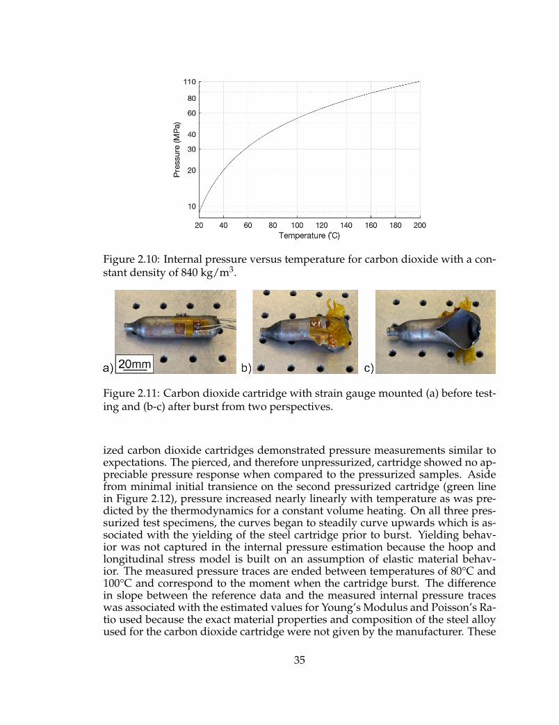
Figure 2.10: Internal pressure versus temperature for carbon dioxide with a con-stant density of 840 kg/m3.

Figure 2.11: Carbon dioxide cartridge with strain gauge mounted (a) before test-ing and (b-c) after burst from two perspectives.

ized carbon dioxide cartridges demonstrated pressure measurements similar toexpectations. The pierced, and therefore unpressurized, cartridge showed no ap-preciable pressure response when compared to the pressurized samples. Asidefrom minimal initial transience on the second pressurized cartridge (green linein Figure 2.12), pressure increased nearly linearly with temperature as was pre-dicted by the thermodynamics for a constant volume heating. On all three pres-surized test specimens, the curves began to steadily curve upwards which is as-sociated with the yielding of the steel cartridge prior to burst. Yielding behav-ior was not captured in the internal pressure estimation because the hoop andlongitudinal stress model is built on an assumption of elastic material behav-ior. The measured pressure traces are ended between temperatures of 80°C and100°C and correspond to the moment when the cartridge burst. The differencein slope between the reference data and the measured internal pressure traceswas associated with the estimated values for Young’s Modulus and Poisson’s Ra-tio used because the exact material properties and composition of the steel alloyused for the carbon dioxide cartridge were not given by the manufacturer. These

35

Figure 2.12: Pressure versus temperature for pressurized and pierced carbondioxide cartridges heated until failure or test fixture temperature limits.

two material properties define a constant coefficient E/(1 + ν) which propor-tionally relates internal pressure to the strain measurements. Differences in thisterm caused a change in slope between the NIST reference and measured pres-sure traces. The majority of the material property uncertainty was attributed tothe potential Young’s Modulus variation which has been reported up to 20% forthin samples of steels of various grades [86]. The slope difference between pre-dicted and measured pressure trends is smaller than this possible 20% variancein material property. In spite of this uncertainty, the general trends between in-ternal pressure and temperature measurements compare well to what would beexpected from a constant volume heating.

The carbon dioxide cartridge validation experiments were significantlyless susceptible to measurement uncertainty than live battery tests. The previ-ously described validation experiment with empty 18650 cases demonstrated anuncertainty band of approximately 0.4 MPa for an unpressurized specimen. Inthe compressed carbon dioxide cartridge validation, the material yielded at aninternal pressure near 40 MPa, but live cells are expected to begin venting near2 MPa. Given the much higher pressure responses from the carbon dioxide car-tridge validation experiments, the results presented here represent a more idealexample of the capabilities of this measurement methodology.

36

CHAPTER 3

RESULTS FROM LIVE 18650 THERMAL ABUSEEXPERIMENTS IN THE INTERNAL PRESSURE

MEASUREMENT CALORIMETER

Live battery abuse tests focused on determining the ability to implementthe internal pressure measurement methodology during thermal abuse testingand quantitatively describing the trends of the internal pressure build up priorto venting onset. LG brand, model HE2 batteries were tested because the lithiumcobalt oxide cathode chemistry has well documented and demonstrated ventingfailures under thermal abuse [13]. LG branded vent caps, generic across multiplecell chemistries, have an experimentally determined burst pressure of 1.906 MPa[9]. The known burst pressure is a reference to evaluate the accuracy of the strain-based internal pressure measurement. State of charge was established at 100%and confirmed prior to testing by collaborators at Sandia National Laboratories,and all cells tested were from the same manufacturing lot for consistency betweentrials. Measuring when and how gas generation occurred prior to venting onsetprovides a deeper understanding of how a battery fails under thermal abuse.

The same stacked strain gauges used in validation trials were bonded tothe four live battery test samples using the same X280 room temperature cur-ing epoxy adhesive along with solder pads for circuit protection and strain re-lief as shown in Figure 3.1(a). Trials were performed at nominal heating ratesof 2.4°C/min, 3.6°C/min, and 4.8°C/min. The highest heating rate test, whichwas the same rate that validation experiments were performed at, was tested induplicate. Tests began at room temperature and were performed until batteryfailure. Venting onset occurred between 138°C and 151°C for all four live celltests, but the vents quickly became clogged and heating was applied until a sec-ond, much larger failure occurred. Strain data was unable to be recorded afterthe initial venting because the strain gauges, and particularly the soldered cir-cuit completion joints, typically failed during the first venting event. Heatingwas applied until the second venting event to ensure that battery decomposi-tion was as complete as possible to minimize the risk to test operators after theexperiment. Batteries vented gas along with a significant amount of solid partic-ulate likely associated with the second failure event which typically melted holesthrough the end of the cell opposite the vent mechanism. After each test, thestrain gauge and electrical connections were completely delaminated from thebattery surface, shown in Figure 3.1(b). Due to the destructive nature of these

37

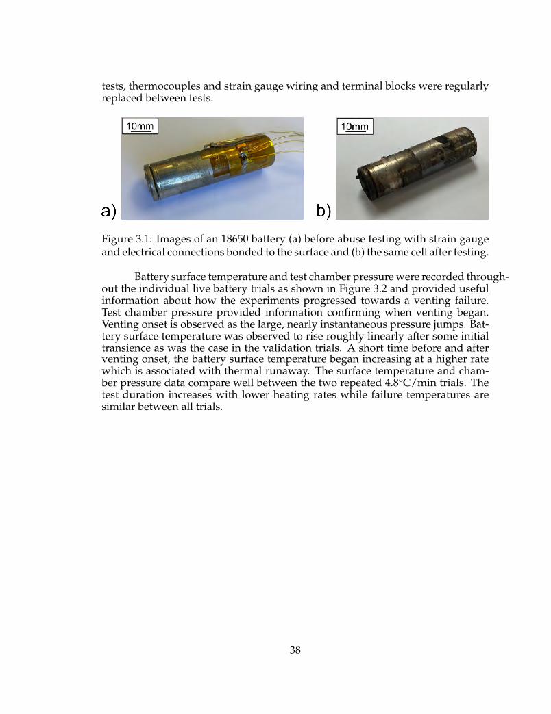
tests, thermocouples and strain gauge wiring and terminal blocks were regularlyreplaced between tests.

Figure 3.1: Images of an 18650 battery (a) before abuse testing with strain gaugeand electrical connections bonded to the surface and (b) the same cell after testing.

Battery surface temperature and test chamber pressure were recorded through-out the individual live battery trials as shown in Figure 3.2 and provided usefulinformation about how the experiments progressed towards a venting failure.Test chamber pressure provided information confirming when venting began.Venting onset is observed as the large, nearly instantaneous pressure jumps. Bat-tery surface temperature was observed to rise roughly linearly after some initialtransience as was the case in the validation trials. A short time before and afterventing onset, the battery surface temperature began increasing at a higher ratewhich is associated with thermal runaway. The surface temperature and cham-ber pressure data compare well between the two repeated 4.8°C/min trials. Thetest duration increases with lower heating rates while failure temperatures aresimilar between all trials.

38

Figure 3.2: Battery surface temperature and test chamber pressure throughoutthe four live battery tests.

39

3.1 Strain measurements from individual tests

Hoop and longitudinal strain measurements were recorded during all fourlive battery thermal abuse tests. Shown in Figures 3.3 through 3.6 hoop andlongitudinal strain values varied widely between individual trials and demon-strate some initial unpredictable behavior before an ultimate rise before failure.All data traces shown have a restricted domain to the moment venting was firstnoted via chamber pressure measurement. After first venting, the strain mea-surement tended to jump between the maximum and minimum of the potentialmeasurement range as determined by the NI cDAQ measurement card. This isindicative of failing electrical connections in the strain gauge circuit completionwhich would coincide with strain gauge delimitation as was observed after allfour live battery tests. Reported internal pressure values were calculated via thethin wall method given the 0.12 mm measured case thickness of the LG brandbatteries and the outer diameter of 18.0 mm.

Figure 3.3: Hoop and longitudinal strain measurements and the correspondingindicated internal pressure for the first 4.8°C/min trial.

40

Figure 3.4: Hoop and longitudinal strain measurements and the correspondingindicated internal pressure for the repeated 4.8°C/min trial.

Figure 3.5: Hoop and longitudinal strain measurements and the correspondingindicated internal pressure for the 3.6°C/min trial.

41

Figure 3.6: Hoop and longitudinal strain measurements and the correspondingindicated internal pressure for the 2.4°C/min trial.

42

All four tests demonstrated some erratic behavior in early strain measure-ments (typically below 100°C). This behavior manifested as an apparent or in-dicated internal pressure build up. Much of these early indicated pressures areclearly non-physical as they reached negative values multiple times larger thanatmospheric pressure. This phenomena is attributed to potential interactionsbetween internal battery components and the case along with relief of residualstresses from the forming process of the battery case. In the higher heating rate ofboth 4.8°C/min tests, these affects appear to have been minimized. While initialstrain measurement trends appeared unpredictable, the difference between thetwo measurements provided the information needed to calculate internal pres-sure and was typically more consistent than individual measurements.

In all tests, a final rise in strain measurements and a growing differencebetween hoop and longitudinal values was noticed. This manifested as a risinginternal battery pressure immediately prior to venting onset. The onset of thispre-venting pressure build up began at different moments for each trial, but allcells showed an accelerating rate of pressure build up until the battery vent ulti-mately opened. The final indicated burst pressure for each trail is listed in Table3.1. Vents from LG branded batteries have an experimentally determined meanburst pressure of 1.906 MPa [9] which is comparable to these final pressures in allbut the 3.6°C/min trial. The uncharacteristically low value for the strain basedburst pressure measurement on this trial is attributed to the large negative in-dicated internal pressure before the final pressure build up. When consideringthe 2.06 MPa difference between the minimum (−1.63 MPa) and final indicatedinternal pressures for this trial, the pressure built up at the end of this trial is com-parable to the burst pressure of an LG brand battery vent. Of note, the spread ofthese measured burst pressures can be accounted for by variability in vent mech-anism burst pressure and the roughly 0.4 MPa measurement uncertainty rangedemonstrated in empty battery case validation experiments.

Table 3.1: Indicated burst vent burst pressureHeating rate Pressure (MPa)4.8°C/min 2.50

4.8°C/min (repeat) 1.843.6°C/min 0.4352.4°C/min 2.16

3.2 Pressure build up versus time and temperature

Due to the wide range of heating rates, the total test duration varied sig-nificantly between trials as shown in Figure 3.7. The final pressure build uptime duration was also longer for lower heating rate tests. Time to failure and

43

Figure 3.7: Comparing indicated internal battery pressure versus time betweenthe four trials.

the beginning of accelerated pressure build up are similar between the repeated4.8°C/min trials.

To demonstrate similarities between the trials in the internal pressure pro-gression leading up to venting, measured pressure build up was plotted againstbattery surface temperature as shown in Figure 3.8. Here, it is clear that all batter-ies began venting at similar temperatures as tabulated in Table 3.2. Additionally,the final pressure rise began in all trials between 80°C and 110 °C. As such, rate offinal pressure build up with respect to temperature was similar between all fourtrials. In all trials, the pressure build up appeared to accelerate somewhat beforeventing onset.

Table 3.2: Battery surface temperature at venting onsetHeating rate Temperature (°C)4.8°C/min 151.3

4.8°C/min (repeat) 150.83.6°C/min 143.22.4°C/min 138.2

3.3 Correlating pressure rise to self heating and thermal runaway

From the battery surface temperature traces first reported above in Figure3.2, careful observation shows a slight upwards concavity to these trends which

44

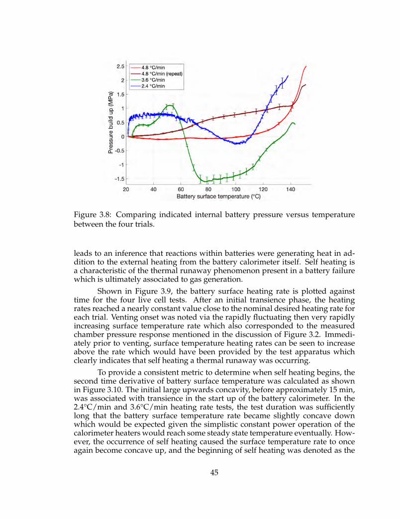
Figure 3.8: Comparing indicated internal battery pressure versus temperaturebetween the four trials.

leads to an inference that reactions within batteries were generating heat in ad-dition to the external heating from the battery calorimeter itself. Self heating isa characteristic of the thermal runaway phenomenon present in a battery failurewhich is ultimately associated to gas generation.

Shown in Figure 3.9, the battery surface heating rate is plotted againsttime for the four live cell tests. After an initial transience phase, the heatingrates reached a nearly constant value close to the nominal desired heating rate foreach trial. Venting onset was noted via the rapidly fluctuating then very rapidlyincreasing surface temperature rate which also corresponded to the measuredchamber pressure response mentioned in the discussion of Figure 3.2. Immedi-ately prior to venting, surface temperature heating rates can be seen to increaseabove the rate which would have been provided by the test apparatus whichclearly indicates that self heating a thermal runaway was occurring.

To provide a consistent metric to determine when self heating begins, thesecond time derivative of battery surface temperature was calculated as shownin Figure 3.10. The initial large upwards concavity, before approximately 15 min,was associated with transience in the start up of the battery calorimeter. In the2.4°C/min and 3.6°C/min heating rate tests, the test duration was sufficientlylong that the battery surface temperature rate became slightly concave downwhich would be expected given the simplistic constant power operation of thecalorimeter heaters would reach some steady state temperature eventually. How-ever, the occurrence of self heating caused the surface temperature rate to onceagain become concave up, and the beginning of self heating was denoted as the

45

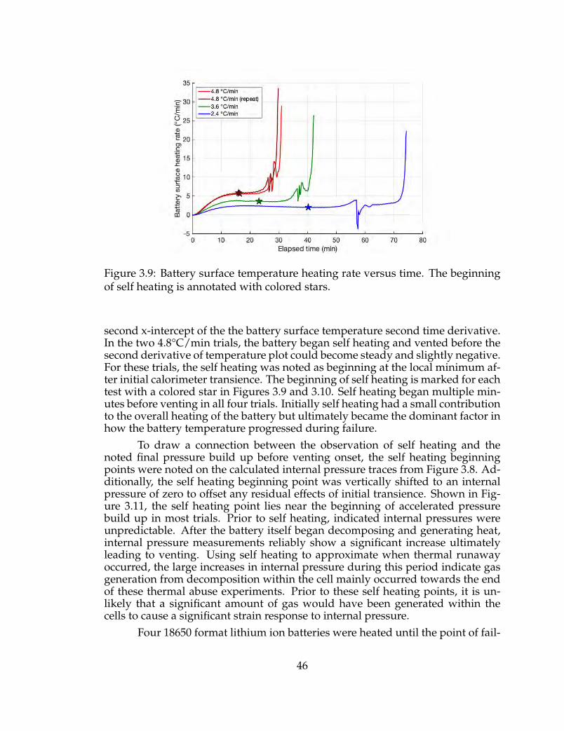
Figure 3.9: Battery surface temperature heating rate versus time. The beginningof self heating is annotated with colored stars.

second x-intercept of the the battery surface temperature second time derivative.In the two 4.8°C/min trials, the battery began self heating and vented before thesecond derivative of temperature plot could become steady and slightly negative.For these trials, the self heating was noted as beginning at the local minimum af-ter initial calorimeter transience. The beginning of self heating is marked for eachtest with a colored star in Figures 3.9 and 3.10. Self heating began multiple min-utes before venting in all four trials. Initially self heating had a small contributionto the overall heating of the battery but ultimately became the dominant factor inhow the battery temperature progressed during failure.

To draw a connection between the observation of self heating and thenoted final pressure build up before venting onset, the self heating beginningpoints were noted on the calculated internal pressure traces from Figure 3.8. Ad-ditionally, the self heating beginning point was vertically shifted to an internalpressure of zero to offset any residual effects of initial transience. Shown in Fig-ure 3.11, the self heating point lies near the beginning of accelerated pressurebuild up in most trials. Prior to self heating, indicated internal pressures wereunpredictable. After the battery itself began decomposing and generating heat,internal pressure measurements reliably show a significant increase ultimatelyleading to venting. Using self heating to approximate when thermal runawayoccurred, the large increases in internal pressure during this period indicate gasgeneration from decomposition within the cell mainly occurred towards the endof these thermal abuse experiments. Prior to these self heating points, it is un-likely that a significant amount of gas would have been generated within thecells to cause a significant strain response to internal pressure.

Four 18650 format lithium ion batteries were heated until the point of fail-

46

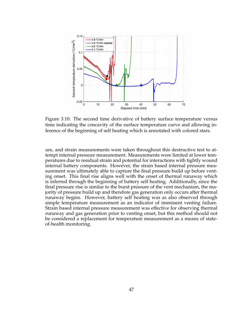
Figure 3.10: The second time derivative of battery surface temperature versustime indicating the concavity of the surface temperature curve and allowing in-ference of the beginning of self heating which is annotated with colored stars.

ure, and strain measurements were taken throughout this destructive test to at-tempt internal pressure measurement. Measurements were limited at lower tem-peratures due to residual strain and potential for interactions with tightly woundinternal battery components. However, the strain based internal pressure mea-surement was ultimately able to capture the final pressure build up before vent-ing onset. This final rise aligns well with the onset of thermal runaway whichis inferred through the beginning of battery self heating. Additionally, since thefinal pressure rise is similar to the burst pressure of the vent mechanism, the ma-jority of pressure build up and therefore gas generation only occurs after thermalrunaway begins. However, battery self heating was as also observed throughsimple temperature measurement as an indicator of imminent venting failure.Strain based internal pressure measurement was effective for observing thermalrunaway and gas generation prior to venting onset, but this method should notbe considered a replacement for temperature measurement as a means of state-of-health monitoring.

47

Figure 3.11: Indicated internal pressure curves with the beginning of self heatingindicated with colored stars. Pressure traces have been vertically shifted so theself heating onset moment lies at zero internal gauge pressure to demonstrate thecomparable magnitude of the final pressure build up between all trials.

48

CHAPTER 4

SIMPLIFIED BATTERY VENTING MODEL FOR INFORMINGFLOW BOUNDARY CONDITIONS

A simplified, one-dimensional venting model is defined here to demon-strate the relation between pressure build up within a finite volume and ventmechanism parameters to describe how pressure varies with time. By predictingcell pressure as a function of time throughout venting, the applicability of the PIVand high speed schlieren experiments may be described.

Previous experimental work at New Mexico Tech by the author has exper-imentally determined the boundary and initial conditions for a simplified tran-sient venting model able to describe the battery internal pressure after burst alongwith mass flow rate [78]. Mean values the statistical distribution of burst pressure(Pb), opening area (Ae), and discharge coefficient (Cd) were measured for ventcaps including the MTI brand vents used here [9]. This model is intended to in-form under what circumstances simulated venting flows may be representativeof actual live cells venting under abuse conditions.

Beginning with conservation of mass within a control volume surroundinga hypothetical venting 18650 format cell, the rate of change of mass containedwithin the battery ( dm

dt ) is equivalent to the negative of the mass flow rate out ofthe cell (mout):

dmdt

= −mout (4.1)

Assuming constant properties within the cell and using the Ideal Gas Law,the mass within the cell is:

m =P0

RT0V (4.2)

where P0 and T0 are the stagnation pressure and temperature, respectively.The pressurized volume of fluid is V which is approximated as 1.52 · 10−6 m3 [47].Taking the time derivative allows rewriting of the left hand side of Equation 4.1:

dmdt

=V

RT0

dP0

dt(4.3)

49

Further, the actual mass flow rate out of the cell is equal to the productof discharge coefficient and the maximum theoretically possible flow rate whichoccurs under isentropic conditions. The right hand side of Equation 4.1 can bewritten as:

mout = Cd ·P0√RT0

Ae√

γMe

(1 +

γ− 12

M2e

) γ+12−2γ

(4.4)

where Me is the Mach number at the vent cap exit. If the ratio of stagna-tion pressure to atmospheric pressure (P0/Patm) is greater than 1.892, the flow ischoked, the Mach number at the vent cap exit is fixed at unity. In this circum-stance, the exit pressure is greater than atmospheric, so the flow is described asunder expanded. At P0/Patm = 1.892, the exit pressure will reach atmosphericpressure and this choked flow is said to be perfectly expanded. Once P0/Patmdrops below 1.892, exit pressure will be assumed to be equal to atmospheric pres-sure and the flow will be un-choked. To calculate the exit Mach number of anun-choked flow the equation:

P0

Patm=

(1 +

γ− 12

M2e

) γγ−1

(4.5)

will be solved for Me.By substituting Equations 4.3 and 4.4 into Equation 4.1 and simplifying, a

differential equation for pressure as a function of time is achieved:

dP0

dt= −Cd ·

P0√

RT0

VAe√

γMe

(1 +

γ− 12

M2e

) γ+12−2γ

(4.6)

The initial condition P0(t = 0) = Pb is applied to determine the singleconstant of integration necessary. Solving this equation as an exponential decaywould be trivial under constant parameters, but previous testing has demon-strated that discharge coefficient is a function of stagnation pressure and the exitMach number clearly changes as the flow becomes un-choked [78, 47]. In practice,Equation 4.6 is solved numerically with a fourth-order Runge-Kutta differentialequation solver in MATLAB (“ode45” function). The mean burst pressure andopening area of MTI brand vent caps are 2.158 MPa and 8.967 mm2 respectively.The mean discharge coefficient profile versus pressure is approximated as a con-stant value of Cd = 0.75 below a normalized stagnation pressure of P0/Patm = 2.2and Cd = 0.95 above P0/Patm = 3.2 with a linearly varying section in the middle.To accommodate for discharge coefficient and Mach number both being piece-wise functions of stagnation pressure, an intermediate function recalculates val-ues for both parameters every time the Runge-Kutta solver calculates dP0/dt. Toavoid complex valued exit Mach number values, Mach number is automaticallyset to zero when stagnation pressure reaches atmospheric pressure. The volume

50

of the pressure reservoir within the battery was approximated as 1.52 cm3 [28].Venting calculations are made with γ = 1.4 representing air and a constant stag-nation temperature of 293 K to represent the steady state gas venting describedin Chapter 7.

Figure 4.1 shows stagnation pressure as a function of time after ventingonset. The region of interest immediately after burst is experimentally simulatedwith the test apparatus described in Chapters 5 and 6. However, as time pro-gresses, the experimental flow no longer accurately represents an actual batteryfailure because gas is still supplied from an upstream pressurized cylinder. Vent-ing at stagnation pressures lower than 345 MPa is simulated by trials at discretestagnation pressure set points. While the burst trials with simulated electrolyteare transient and multiphase in nature, these steady, fixed point gas venting ex-periments provide accurate velocity distributions without the flow field. By test-ing under steady conditions, trial length can be as long as desired which allowsenough data to be recorded to accurately quantify the mean velocity field andturbulence strength.

Figure 4.1: Battery internal pressure versus time after burst showing the regionsin which the current vent burst and steady state PIV experiments are applicable.

51

CHAPTER 5

OPTICAL MEASUREMENT TECHNIQUES FOR TRANSIENT,MULTIPHASE VENTING FLOW

5.1 Principals of high speed schlieren and equipment used

Schlieren imaging is a technique within a family of flow visualization meth-ods including shadowgraphy and background oriented schlieren which allow thevisualization of changes in refractive index within a transparent media [89]. Inthe case of gaseous flows, index of refraction disturbances are generally causedby variable density or multiple gas species. As such, schlieren and the otherrefractive imaging techniques are able to visualize flow features such as shockwaves and compressible turbulence with density gradients or mixing betweenmultiple gas species. For a gas, refractive index varies linearly with density viathe Gladstone-Dale Law:

n = kρ + 1 (5.1)

where n is the index of refraction, k is a material constant which varies bychemical species, and ρ is density.

A parallel-light schlieren system was implemented here for visualizing gasventing from battery cells, as depicted in Figure 5.1(a). Light from a point sourceplaced at the focal length of a convex lens was collimated into a test section wherethe simulated battery venting test fixture was placed. Beyond the collimated testsection, a second convex lens collects the light and refocuses it to a point. Atthis point, a knife edge is carefully placed to block approximately half of the lightbefore it enters the high-speed camera’s lens. Since the knife edge cutoff is placedat the focus of the light, it does not distort the image the camera collects but ratherprovides an even darkening effect throughout the field of view. When a schlierenobject (a feature which refracts light) is introduced to the test section, the refractedlight rays will focus to a different location. Light which focuses on the knife edgecreates dark regions within images while the refracted light which now misses thecutoff creates light regions. This leads to the light-to-dark gradients across flowstructures which is characteristic to schlieren images as shown in Figure 5.1(b). Ofnote, opaque regions within the test section block light and appear black withinschlieren images. Schlieren imaging can be performed without the need for aspecialized camera and provides intuitively-understandable flow visualizationswhich allow various measurements and insights into flow features.

52

Figure 5.1: (a) A schematic representation of the schlieren setup used, and (b) arepresentative image of the schlieren images recorded of simulated battery vent-ing.

All schlieren images recorded in this work were taken with a Photron SA-X2 high speed digital camera. Camera resolution was set to 384 by 584 pixels (px)with a spatial calibration between 0.1 mm/px and 0.15 mm/px depending on theindividual trial and camera lens focal length. Images were generally recorded ata frame rate of 48 kHz with an exposure of 0.29 µs, but this was changed asneeded. The lenses used to collimate and collect light were a matched pair of127-mm-diameter parabolic telescope objectives with an aperture of f /5. Pointsource illumination was provided by a SugarCUBE brand light emitting diode(LED) illuminator with adjustable intensity output.

Here, carbon dioxide was chosen as a substitute for the mixture of gasespresent in battery venting as it is generally the most prevalent species withinthese flows without being combustable or highly toxic. Depending on cell chem-istry, carbon dioxide has been measured to account for between 24.9% and 53.0%of vented gas material [28]. The other significant components of gas venting arehydrogen and carbon monoxide. Carbon dioxide also has the added benefit ofhaving relatively high visibility in schlieren imaging in an air atmosphere.

5.2 Vent cap burst fixture with visualization capability

Intact vent caps, sourced as components, are placed within the vent burstpressure test fixture shown installed in the laboratory in Figure 5.2(a). The fixturewas designed and fabricated predominantly from commercially available off-the-shelf components for simplicity. The vent cap is placed within a parallel lightschlieren system for visualization of both gas and liquid components of the flow.

Brass and steel pipe fittings were used to construct the vent cap hold-ing fixture without needing complicated machining. Carbon dioxide is suppliedfrom a siphon-less compressed gas cylinder via a 12.7 mm outer diameter tubewhich is connected to the fixture with a stainless steel Swagelok tube fitting.The gas supply was then directed through a ball valve to the main fixture body.

53

Figure 5.2: (a) The burst fixture installed in the laboratory, and (b) a schematic ofthe setup showing the construction of the vent holder and the field of view.

This main structure was constructed from galvanized steel pipe nipples and Teeswhich allow for pressure measurement ports. The ball valve was used to stop theflow of gas once the vent cap opened to end the test, but it is left open duringtesting. All pipe fittings used either tapered NPT threads or Swagelok style com-pression fittings, up to the main body of the fixture, after which straight threadswere used to allow variability in vent cap thickness.

A brass 3/8 NPT to 1-8 UNC straight thread fitting with a custom designedaluminum cap was used to secure the battery vent cap. A silicone gasket andlaser cut acrylic gasket retaining ring are placed adjacent to the vent cap to createa seal for the pressurized gas prior to burst. A cutaway model view of the testapparatus is shown in Figure 5.2(b). The aluminum cap was machined to hold thevent cap in place while minimizing obstructions within the field of view adjacentto the vent openings. The only obstructions within the field of view are the twocantilevered tabs on the holding ring which keep the vent cap sealed against thesilicone gasket. These tabs also provide a spatial calibration as their outer cornersare 25.4 mm apart. The front of the vent cap sits 0.5 mm past the front of thecompression nut to ensure that the test apparatus is minimally obstructing thefield of view.

The vent cap holding fixture was mounted to an acrylic plate which is sup-ported by four posts on an optical table. A length of high-pressure rated nylontubing connects the vent cap holder to the compressed air supply which can beregulated between 0 MPa and 3.45 MPa. The pressure regulator was operatedmanually to increase pressure to failure during testing, and a dial type pressuregauge was used on the outlet of the regulator to confirm the reading from thepressure transducer installed on the vent cap holder. A follower-hand on thedownstream pressure gauge showed the maximum pressure in each test, corre-sponding to the vent burst pressure. A compressed air cylinder was used for vent

54

testing as it could supply sufficiently high pressures.

5.3 Sucrose solution as an electrolyte substitute

Common liquid electrolytes in lithium ion batteries contain mixtures of or-ganic hydrocarbons such as ethylene carbonate, dimethyl carbonate, and propy-lene carbonate [33]. To avoid flammability concerns with using these compounds,sucrose solutions were tailored to match individual properties of ethylene car-bonate. Exact electrolyte formulations are generally proprietary and differing be-tween different cell chemistries and manufacturers, so the simulated electrolyteis formulated to roughly approximate electrolyte spray characteristics while mea-surement techniques are being developed. Table 5.1 compares the applicablefluid dynamic properties of ethylene carbonate to the two sucrose solution mix-tures [90, 91, 92]. Both sucrose solutions were created in warmed, distilled waterwith a small amount of food coloring to promote differentiation from gas ventingin schlieren images and sucrose.

Table 5.1: Properties of ethylene carbonate electrolyte and sucrose solutionsSample Density (g/cm3) Viscosity (cP)

Ethylene carbonate 1.34 2.5626% sucrose/water 1.11 2.5769% sucrose/water 1.34 329

While no sucrose solution will provide perfect similarity to hydrocarbonelectrolytes, the different mixtures were compared to evaluate which parameterwas most critical for matching the results in previous schlieren imaging of livebattery failures. Figure 5.3 shows schlieren images of simulated vent burst com-pared to a live cell failure at approximately 2.8 ms after burst. Both the 26%sucrose solution and the live cell failure show a similar spray with clear atomiza-tion while the 69% sucrose solution shows droplet breakup characteristics of thesecond wind-induced regime. The main visually observable differences betweenthese two flow regimes is the different droplet sizes where atomized particleswere significantly smaller than those in the second wind-induced regime [58].The wind-blown particles in Figure 5.3(c) also demonstrated breakup outside ofthe vent orifice and at downstream locations in the flow [59]. Atomized flowbroke apart at the orifice itself [59].

55

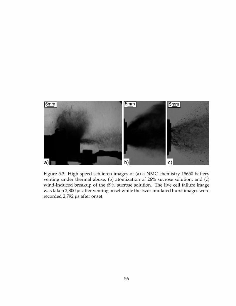
Figure 5.3: High speed schlieren images of (a) a NMC chemistry 18650 batteryventing under thermal abuse, (b) atomization of 26% sucrose solution, and (c)wind-induced breakup of the 69% sucrose solution. The live cell failure imagewas taken 2,800 µs after venting onset while the two simulated burst images wererecorded 2,792 µs after onset.

56

CHAPTER 6

EXPERIMENTAL RESULTS AND DATA ANALYSIS OFSIMULATED VENTING EXPERIMENTS

Using the previously described vent burst testing fixture and high speedschlieren imaging technique, experiments were conducted to:

• Determine how the introduction of a liquid phase affects the velocity, flowfront penetration, and spreading rate of transient venting flow.

• Characterize the fundamental transient, multiphase fluid dynamics of theflow field created by multiple jets issuing from a finite volume, pressurizedreservoir.

Three trials were performed to evaluate the role of the liquid componentin venting flow immediately after vent mechanism burst: a baseline gas ventingcase and two trials with sucrose solutions which simulate the electrolyte portionof venting. In these experiments, carbon dioxide was used as the gas compo-nent of the venting flow for improved visibility in the schlieren imaging and toreplicate the properties of gases vented from batteries. The initial portion of theventing flow represents the transience associated vent burst, but, unlike ventingfrom a finite volume, experiments reach a steady state venting condition oncegas flow becomes choked within the upstream pressure regulator. As such, theseexperiments are only representative of battery venting in early time scales.

All trials were performed with the vent cap in a vertical orientation toallow even spread of the 1 mL of simulated electrolyte against the burst disk.The schematic representation of the text fixture seen in Figure 5.2(b) shows howthe schlieren field of view is reported in data throughout this chapter, but Figure6.1 shows how the fixture was oriented in the lab and the location of the sucrosesolution before vent burst. Care was taken to pipette the sucrose solution directlyonto the burst disk rather than the inner surface of the test fixture, and the initialdepth of the liquid was 6.1 mm.

The baseline trial, with a series of recorded schlieren imaging frames inFigures 6.2 and 6.3, had clearly identifiable individual jets correlated to the lo-cation of each of the openings in the vent’s electrical terminal. Imaged with acollimated light schlieren setup, this image is the path integrated refraction oflight passing through the test section. The image appears to show three individ-ual jets, one directed upward, downward, and horizontally. The horizontal jet is

57

Figure 6.1: Schematic cross section showing the location of the sucrose solutionwithin vent burst test apparatus prior to venting onset.

actually the projection of the two separate jets which are aligned in this viewingorientation. The parallel light schlieren system precludes any depth resolution inthe image so the jets appear as one combined jet. The initial image series in Fig-ure 6.2 shows the initial formation of the individual jets along with a weak shockwave associated with the opening of the burst disk. In the later timescales shownin Figure 6.3, jetting appears to have consistent projection and spreading anglesonce the flow has established.

Figure 6.2: High speed schlieren images from gas-only burst trial showing theinitial jet propagation into the environment.

The other two tests vented the sucrose solutions described in Section 5.3along with gaseous carbon dioxide. Shown in Figure 6.3, the low viscosity su-crose solution formed an atomized spray while the larger droplets of the highviscosity solution with ligament formation is characteristic of the second wind-induced breakup regime [58]. Both flows showed a droplet spray that was ini-tially wider in the radial direction than gas venting alone, but the droplet spraywas continually narrowing as the liquid within each cap was vented. After the

58

sucrose solutions were vented, the gas venting established with steady projectionand spreading angles similar to the gas-only trial. Unevenness, as noted in thebottom jet from the low viscosity solution trial, is attributed to the burst disk re-maining attached within the vent mechanism at a single point which blocked aportion of the corresponding opening in the vent’s electrical terminal. The indi-vidual droplets in the atomized spray were too small to be resolved individually,but these particles were densely populated and darkened the schlieren images.The atomized flow blocked schlieren visibility until most of the liquid withinthe vent had been exhausted. The high viscosity wind-induced flow performedsimilarly, but larger gaps between particles allowed more visibility for the gascomponent of the flow.

59

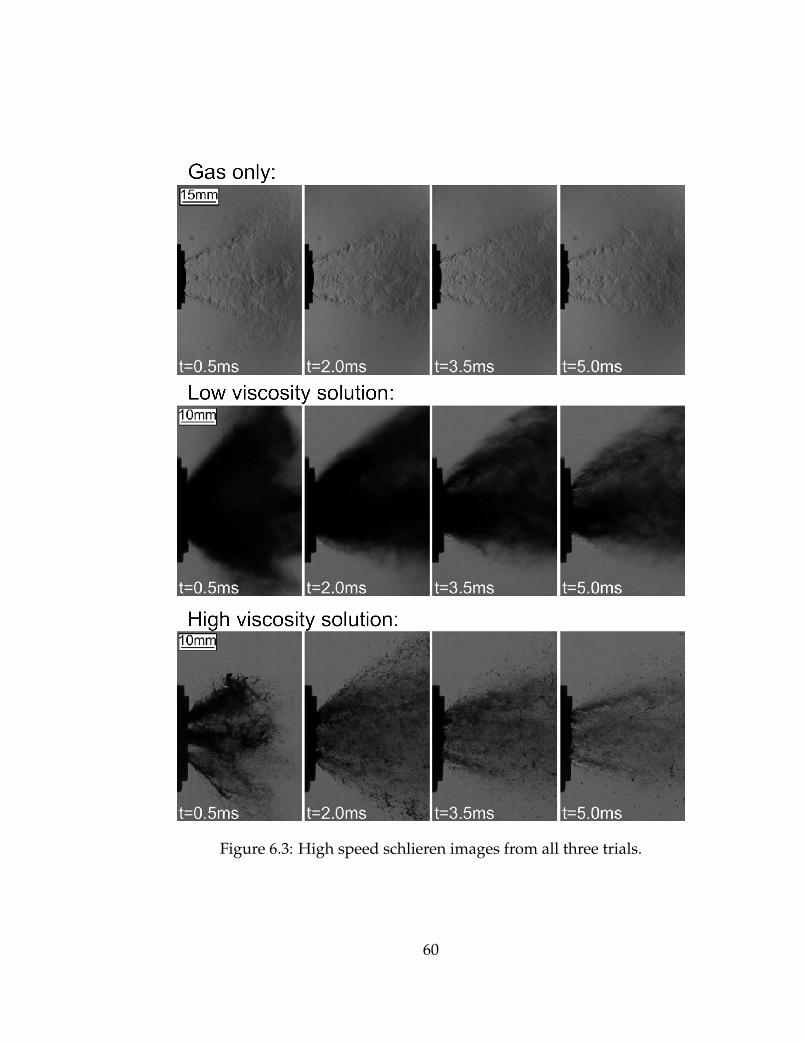
Figure 6.3: High speed schlieren images from all three trials.

60

An image processing routine was written in MATLAB to isolate the liquidventing components from the gas within the high speed schlieren images. Theability to distinguish between liquid and gas portions of the flow is necessaryto understand the fluid dynamics of multiphase venting. Liquid droplets willinteract with the flow and carry momentum in different ways based on the sprayregime and the corresponding particle sizes. From a battery safety perspective,flammable electrolyte droplets also contain significant chemical potential energyand may coat surfaces near venting cells.

A mean gas flow image was created from the steady venting portion ofthe high speed schlieren image sets after the carbon dioxide portion of the flowchoked within the regulator. This was mean image is calculated via pixel by pixelaveraging from 480 schlieren images for each trial since there were slight flowfield differences related to unpredictable burst disk opening characteristics. Thismean flow image was then subtracted from each transient test image to minimizethe intensity of the schlieren effect caused by the gas flow. To be able to visualizethese mean-subtracted images, pixel intensities were rescaled such that no changebetween the transient and mean images was represented a 50% gray. The darkestregions of these subtracted images were isolated as they represent the location ofthe liquid droplets. These liquid portions of the flow were then highlighted withred pixels. If the intensity difference between the mean schlieren gas venting andthe transient spray image at a given pixel location was larger than 0.1, the flowwas assumed to be liquid. The steps of this image processing routine are shownin Figure 6.4.

Figure 6.4: Liquid detection image processing steps including (a) raw steady-state schlieren images, (b) mean steady gas venting, (c) multiphase venting imagewith mean schlieren subtracted, and (d) liquid portions of the flow determined bythresholding (c) and highlighting in red. The raw droplet spray image processedin parts (c) and (d) is the low viscosity, t = 5.0 ms frame shown in Figure 6.3.

Streak images were created to analyze how the venting flow changed withtime along one-dimensional axes within the recorded schlieren images. Streakimages are compiled by removing the same row or column of interest (some-times along with adjacent rows or columns to visually assist with distinguishing

61

flow features) from successive high speed images [93]. These one-dimensionalimage intensity vectors are then concatenated into a larger image which repre-sents position on one axis and time on the other as shown in Figure 6.5.

Figure 6.5: (a) Single high speed image of the flow identifying axial and radiallocations where streak images are created, and (b) a radial streak image createdfrom the column at Lc = 10.

Streak images were created from the high-speed schlieren images alongthe axial direction and radial direction, perpendicular to the vent exits. A charac-teristic length Lc scale has been defined:

Lc =

√Ae

njets(6.1)

for the MTI brand vent caps tested. With an exit area (Ae) of 8.967 mm2

and number of jets (njets) of 4, the characteristic length is 1.497 mm2. Relativelocations for 2Lc, 10Lc, and 18Lc are shown in Figure 6.5(a).

Figure 6.6 compares the radial streak images created from the high speedschlieren images recorded in the three simulated vent burst trials. Gas jet pro-jection and spreading angles were constant through time which was visualizedas horizontal bands in the streak images. From further inspection, gas spread-ing and projection, when discernible from the liquid portion of the flow, wereunaffected by the introduction of the droplet spray.

Projection and jet spreading angles are calculated by noting the verticallocation of the center and edges of the jets within streak images in Figure 6.6 atdifferent known distances from the vent cap. The gas experiment was used todetermine the outward projection of the jets which was measured at 21° fromthe axial direction normal to the vent cap. The individual gas jet width spreadingangle was measured as 12°. From this, the entire gas flow field spreads within acone with a full angle of 66°.

62

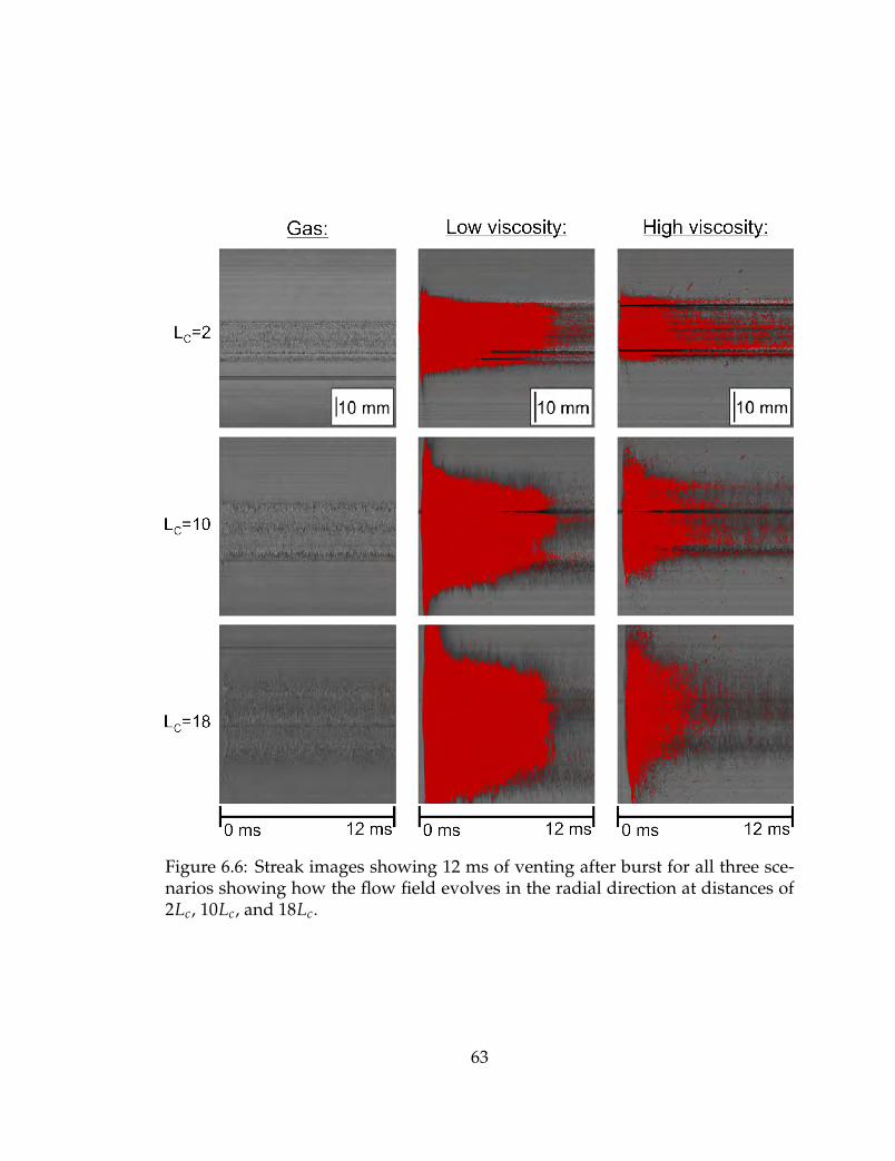
Figure 6.6: Streak images showing 12 ms of venting after burst for all three sce-narios showing how the flow field evolves in the radial direction at distances of2Lc, 10Lc, and 18Lc.

63

For both trials with a liquid component to the venting flow, the streak im-ages in Figure 6.6 demonstrate that droplet spray governed the extent of the flowfield and initial penetration into the quiescent environment. Generally, the lowviscosity, atomized spray was wider than the high viscosity, wind-blown spray.As time progressed and the amount of liquid remaining in the burst pressuretest fixture decreased, the flow field became less densely populated by liquiddroplets. Even though the total width of the initial droplet spray was greaterthan the gas venting radial width, the droplet spray narrowed with time, even-tually tending to a spreading angle of zero as the liquid was exhausted. Sincethe liquid spray width was decreasing with time while the gas venting remainedconstant, the outer edge of the entire flow field transitioned from being com-prised of droplets to gas at 2.5 ms and 5.0 ms after burst for the high viscosityand low viscosity trials, respectively. Qualitatively, the low viscosity, atomizedspray occupied more of the flow field for longer than the high viscosity, wind-blown spray.

Unlike the gas venting case, the liquid spreading angle clearly varies sig-nificantly with time as seen in the streak images in Figure 6.6. Here liquid spread-ing angle (θL) was calculated as the tip angle of a cone enveloping the dropletspray at a distance of 10Lc and a was calculated as:

tan(

θL

2

)=

0.5 · (Droplet Spray Width)10Lc

(6.2)

The distance of 10Lc was chosen because it this was the furthest down-stream location where both trials’ droplet spray remained within the camerafield-of-view. The droplet spray width is defined as the radial distance betweenthe top and bottom edges of the detected liquid spray at a given time. The spread-ing angle of a cone bounding the entire flow is shown in Figure 6.7. The initial riseof spray angle was due to the fact that the spray angle measurement was taken ata distance of 10Lc from the vent cap. These values simply represent the center jetpenetrating to this distance. Once the maximum spray angle measurement wasreached, droplet spray angle steadily decreased with time until the liquid com-ponent of the venting was exhausted. Both sucrose solutions exhibited nearlyidentical total venting time suggesting that viscosity and density variation didnot significantly affect the liquid flow rate. Throughout venting, the low viscos-ity solution demonstrated a wider spray than the high viscosity solution which isdirectly associated with the differences in the two demonstrated spray regimes.This was consistent with previous experimental work which noted higher con-centrations of high Stokes number particles closer to the center of a jet whilelower Stokes number particles spread further towards the edges of the jet [63].The larger droplets from the high viscosity spray showed some spray angle oscil-lations later in the venting process while the atomized flow was more consistentin the spray angle decrease.

To evaluate spray penetration into the quiescent environment immediatelyafter burst, the axial streak images created from the vent centerline row were usedto track the flow front. Of note, the venting flow front is comprised entirely of

64

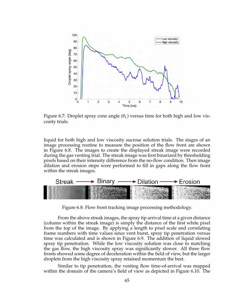
Figure 6.7: Droplet spray cone angle (θL) versus time for both high and low vis-cosity trials.

liquid for both high and low viscosity sucrose solution trials. The stages of animage processing routine to measure the position of the flow front are shownin Figure 6.8. The images to create the displayed streak image were recordedduring the gas venting trial. The streak image was first binarized by thresholdingpixels based on their intensity difference from the no-flow condition. Then imagedilation and erosion steps were performed to fill in gaps along the flow frontwithin the streak images.

Figure 6.8: Flow front tracking image processing methodology.

From the above streak images, the spray tip arrival time at a given distance(column within the streak image) is simply the distance of the first white pixelfrom the top of the image. By applying a length to pixel scale and correlatingframe numbers with time values since vent burst, spray tip penetration versustime was calculated and is shown in Figure 6.9. The addition of liquid slowedspray tip penetration. While the low viscosity solution was close to matchingthe gas flow, the high viscosity spray was significantly slower. All three flowfronts showed some degree of deceleration within the field of view, but the largerdroplets from the high viscosity spray retained momentum the best.

Similar to tip penetration, the venting flow time-of-arrival was mappedwithin the domain of the camera’s field of view as depicted in Figure 6.10. The

65

Figure 6.9: Flow front propagation through time for three burst scenarios.

same trends noted in the axial spray tip penetration measurements were notedfor the full-field time-of-arrival plot. The gas and low viscosity venting flowswere observed to establish the extent of their flow field within approximately0.5 ms while the high viscosity flow took closer to 1 ms. Of note, the later timeof arrival between and at the edges jets in the gas flow field was due to turbulentfluctuations in the flow field.

Figure 6.10: Time-of-arrival maps depicting when venting flow was first noted ata given location near the vent cap.

66

CHAPTER 7

PARTICLE IMAGE VELOCIMETRY (PIV) MEASUREMENTFOR STEADY MULTIPLE-JET VENTING FLOW

7.1 Steady state gas venting test apparatus

Steady state, simulated gas venting experiments are performed with a testapparatus specifically designed and fabricated for use with 18650 format ventcaps and custom geometry orifice plates. While the experiments presented inChapter 9 only utilize orifice plates, the laboratory system was designed withmodularity and robust capabilities for future experiments beyond the scope ofthis body of work. The majority of the test apparatus and associated fixturesare constructed from off-the-shelf components, but custom-fabricated parts weremade where necessary.

Major components of this fixture include the orifice plate or vent cap holder,stilling chamber, and two chamber inlet flow paths as identified in Figure 7.1. Inone inlet, particle seeded air for PIV is supplied from compressed air which flowsthrough an atomizer containing a reservoir of olive oil. The other inlet suppliesdry compressed air from gas cylinders at the flow rates required to maintainsteady venting. The test apparatus is centered around a 74.3 L stilling cham-ber which allows precise measurement of stagnation properties, mixing betweenboth inlet flows, and allows for a simple and short flow path for the acceleratedflow to pass through before exiting the fixture. Throughout the test apparatus,care is made to minimize the length of tubing to minimize frictional losses whichallows the assumption of isentropic flow to remain accurate. The stilling chamberdry air inlet and venting outlet use high flow coefficient ball valves to minimizefrictional losses as well. All cross sections are much larger than the opening areaof a typical 18650 vent cap to ensure that flow is choked at the exit of the vent it-self, and all orifice plates have opening areas smaller than the typical 18650 vent.

Dry air is supplied to the stilling chamber separately from the particleseeded flow because of the relatively high flow rates required for steady opera-tion. Compressed air is used in testing to minimize cost and health considerationswhile still simulating the fluid dynamics of battery venting. A low humidity sup-ply is used as initial testing with compressed, un-dried air showed a tendency forwater to freeze at the vent cap openings due to the drop in temperature as the gasis accelerated. To achieve the desired flow rates through a single pressure regula-tor, high pressure gas cylinders are used. Supply pressure effect, where regulator

67

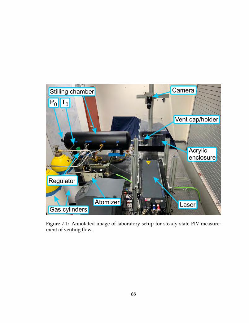
Figure 7.1: Annotated image of laboratory setup for steady state PIV measure-ment of venting flow.

68

output pressure increases as upstream pressure decreases, is reduced by using amanifold of two K-size gas cylinders each with an internal volume of 49.9 L.

Since gas flow must be able to be supplied at various pressures to accu-rately represent battery venting, a pressure regulator was specified to meet theflow rate requirements without itself choking the flow. An upper limit to systemflow rate demands was calculated with isentropic flow relations. Opening areasconsidered include the mean, minimum, and maximum seen in previous MaterialTechnology International Corporation (MTI) brand vent cap testing with valuesof 8.967 mm2, 7.845 mm2, and 9.773 mm2 respectively. Stagnation temperaturewas 20 °C, and atmospheric pressure was 86 kPa measured at the laboratory lo-cated at a 1,400 m elevation. A Swagelok high sensitivity, high flow rate regulator(model KHF1FRF818A20000) with a 0 kPa to 689 kPa control range was used inthese experiments. Figure 7.2 shows the system requirements at various stagna-tion pressure set points (within the stilling tank) compared to the maximum pos-sible flow rate through the regulator with an upstream gas cylinder pressure of3.45 MPa or higher. Per the manufacturer datasheet, maximum flow rates wereinterpolated between known points [94]. At stagnation pressure ratios greaterthan 1.2, the regulator will not choke the flow. However, lower stagnation pres-sures cause the regulator to choke before enough flow is supplied to the stillingchamber. At lower, unchoked stagnation pressures a different two-stage pres-sure regulator (Swagelok model KCY1DRF412A0000) was used for more precisecontrol and to avoid lock up issues associated with the lower flow rates.

Figure 7.2: Flow rate requirements for steady state venting as a function of nor-malized stagnation pressure.

To demonstrate the steady state capability of the test apparatus, Figure 7.3shows a plot of stagnation pressure versus time. Both dry air and particle laden

69

streams were simultaneously run through an MTI brand vent cap. After open-ing the outlet valve on the stilling tank, steady state venting was achieved after35 s. Over the 35.8 s duration of the steady state venting, a mean absolute stag-nation pressure of 261.6 kPa was recorded with a standard deviation of 0.20 kPa.Small steps in pressure of around 0.35 kPa, distinctly larger than the measure-ment resolution, are noticed to occur every 5 to 10 s, but these are negligible whencompared to the standard deviation of the pressure measurements. Further, nopressure change from the initial 10.3 MPa was discernible on the analog pressuregauge attached to the compressed air cylinders. Due to supply pressure effect,the regulator outlet pressure increases as the upstream pressure reservoir in thecompressed gas cylinders is depleted. This causes stagnation pressure to increaseby approximately 1.75 Pa/s as determined by a linear regression fit to the pres-sure data. The rate of stagnation pressure increase is insignificant compared tothe standard deviation in the data. Of note, this rate is ultimately a function ofregulator set point, flow rate, and gas cylinder pressure.

Figure 7.3: Stagnation pressure versus time from the experiment measuring thesteady state gas venting. After t = 0 the flow was steady.

Ample particle seeding is necessary for PIV measurements. The stillingchamber is continuously supplied with particles during venting. The environ-ment surrounding the vent cap was also seeded with tracer particles to aid ve-locity measurements near the periphery of the flow. Seeding in the environmentprior to each trial allows for measurements of entrained flow and provides bettervisualization of the edges of the gas jets. Environment seeding is performed witha flexible tube connected off of a Tee fitting from the main droplet supply to thestilling chamber. This particle flow is selectable with a ball valve, and a needlevalve allows variable flow rate.

Olive oil droplets are chosen as the seed particles for battery venting ex-

70

periments because of their low Stokes number, favorable light scattering, andlack of health hazards after test operator inhalation. The Stokes number for theparticles in the flow is:

Stk =ρpd2

pU18µL

(7.1)

The olive oil droplets have a density (ρp) of 0.911 g/mL and diameter (dp)of approximately 1 µm, resulting in a Stokes number of 0.56 at the sonic ventcap exit which implies a velocity measurement uncertainty of approximately 6%[68]. As the flow decelerates further from the vent cap exit, the accuracy of thistracking is expected to increase significantly because the free-stream velocity de-creases, thus decreasing the local Stokes number. The orifice Stokes number cal-culated here uses an opening diameter as the length scale to describe a turbulentjet. Since there are four openings in the positive terminal of an 18650 vent cap,the jet diameter is taken to be 1.69 mm, which is calculated for a circle with anarea equivalent to one fourth of the mean opening (8.97 mm2) of an MTI brandvent.

Droplets are formed via atomization using a Thermo-Systems Engineer-ing Co. (TSI) Model 9306 atomizer. This atomizer implements six selectableliquid jets which are impinged by a high velocity air jet. Droplets are formedwhen the liquid is then impacted against a spherical impactor [95]. This atom-izer features air pressure regulation and dilution. Dilution is typically adjustedbetween 5 and 10 L/min. The pressure is regulated to a maximum gauge pres-sure of 320 kPa. This pressure setting provides the upper limit of the steady stateventing experiments as stagnation pressure within the stilling tank must be lowerthan the atomizer outlet pressure to ensure continuous seeding. The atomizer hasbeen modified here with a plug blocking the typical output in favor of using anadjacent fill port with NPT threading to simplify piping connections. This mod-ification allows the atomizer to be used in this pressurized system which is notpossible in the factory configuration.

An acrylic enclosure has been fabricated to contain the venting flow andthe dispersal of the olive oil droplets. This enclosure also assists in minimizingunintended flow fields caused by drafts or heating, ventilation, and air condi-tioning flows in the laboratory. Shown in Figure 7.4(a), the acrylic PIV enclosureis 533 mm tall, 537 mm wide, and 349 mm in the vent’s axial direction. The enclo-sure is sized specifically to not interfere with the venting flow using a 21° center-line projection angle and 12° spreading angle. These angles were measured withhigh speed schlieren imaging and are further discussed in the results portionsof this document. A slit is incorporated into the side of the enclosure to allowthe laser sheet illumination to pass into the enclosure with no distortion. Blackvelvet flocking material within the enclosure minimizes laser sheet reflections.Height and tilt adjustments are incorporated into the design of the enclosure foralignment with the vent cap and laser sheet. Both the anticipated venting regionsand the location of the laser sheet are shown in Figure 7.4(b). On the far side of

71

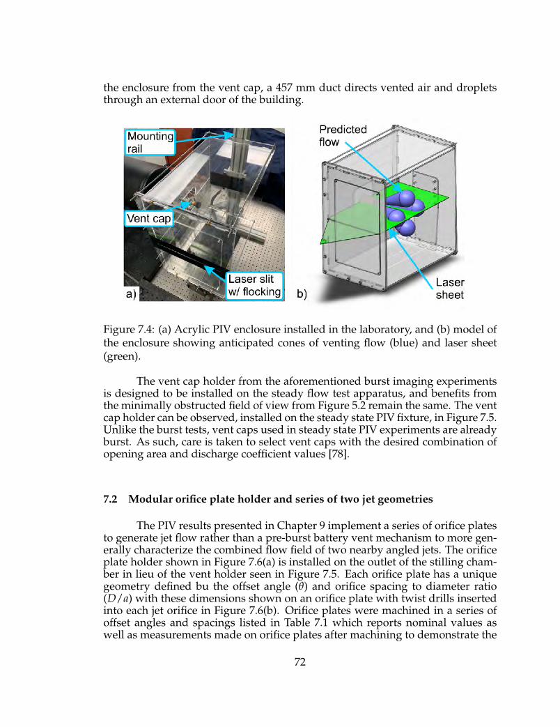
the enclosure from the vent cap, a 457 mm duct directs vented air and dropletsthrough an external door of the building.

Figure 7.4: (a) Acrylic PIV enclosure installed in the laboratory, and (b) model ofthe enclosure showing anticipated cones of venting flow (blue) and laser sheet(green).

The vent cap holder from the aforementioned burst imaging experimentsis designed to be installed on the steady flow test apparatus, and benefits fromthe minimally obstructed field of view from Figure 5.2 remain the same. The ventcap holder can be observed, installed on the steady state PIV fixture, in Figure 7.5.Unlike the burst tests, vent caps used in steady state PIV experiments are alreadyburst. As such, care is taken to select vent caps with the desired combination ofopening area and discharge coefficient values [78].

7.2 Modular orifice plate holder and series of two jet geometries

The PIV results presented in Chapter 9 implement a series of orifice platesto generate jet flow rather than a pre-burst battery vent mechanism to more gen-erally characterize the combined flow field of two nearby angled jets. The orificeplate holder shown in Figure 7.6(a) is installed on the outlet of the stilling cham-ber in lieu of the vent holder seen in Figure 7.5. Each orifice plate has a uniquegeometry defined bu the offset angle (θ) and orifice spacing to diameter ratio(D/a) with these dimensions shown on an orifice plate with twist drills insertedinto each jet orifice in Figure 7.6(b). Orifice plates were machined in a series ofoffset angles and spacings listed in Table 7.1 which reports nominal values aswell as measurements made on orifice plates after machining to demonstrate the

72

Figure 7.5: Vent cap holder installed on steady state PIV test fixture.

accuracy of the machining. With the exception of one 1.70 mm diameter singlejet plate used as a baseline experiment, each orifice plate was machined with twocircular orifices with diameters (a) of 1.70 mm. A three orifice diameter long cir-cular flow path connects each orifice to an internal plenum which matches thecross section of the upstream orifice plate holder. A short internal flow path waschosen to minimize any boundary layer growth inside these internal channelswhile leaving enough thickness for the orifice plate to be mechanically robust.Each jet orifice and the corresponding interior flow path was machined with aNumber 51 twist drill, and all sharp, machined edges were left intact. Orificeplates were attached to the test apparatus with four machine screws, and the sys-tem was sealed with a laser cut silicone gasket. Washers on each screw betweenthe plate holder and the back side of the orifice plate provided a physical stopfor consistent gasket compression and plate alignment with the remainder of theexperimental setup. The jet interaction study was limited to two jet configura-tions rather than the four jets seen on battery vents to provide a more simplifiedscenario which is more appropriately captured with the light sheet illuminationshown in Figure 7.4(b).

Of note, the orifice diameter was chosen to match the opening area of oneof the four jets present on an 18650 format battery vent. Vent mechanisms fromthese batteries have a spacing of approximately six diameters (D/a = 6), and anoffset angle close to 40°. The orifice plates listed in Table 7.1 explore the effectof increased or decreased spacing and the effect of smaller offset angles. Offsetangles up to 40°are not reported because initial investigation showed no inter-action at such a large offset angle, and no interaction is predicted at all of the30°examples as explained in Chapter 8.

The orifice holder has a large flow path with gradual cross section changes

73

Figure 7.6: Annotated images of (a) the orifice plate holder installed in the labora-tory and (b) an orifice plate with two twist drills inserted into the plate’s openingsto show the jet spacing (D/a) and offset angle (θ).

Table 7.1: Two jet orifice plate configurationsNominal spacing Nominal offset angle Measured spacing Measured offset angle

D/a θ D/a θ

3 0 3.05 -0.023 10 3.06 10.43 20 3.01 19.83 30 2.99 29.76 0 6.05 -0.066 10 6.04 10.16 20 6.01 19.86 30 5.97 29.5

12 0 12.01 -0.2212 10 12.00 9.9112 20 12.04 20.012 30 12.04 Not measured

74

prior to the orifice plate exit to minimize losses. The base plane of the orificeplates were extended with a large, circular piece of laser cut acrylic covered inblack velvet material to minimize laser reflection. The additional base plane isused to limit the effects of any entrainment through the back of the acrylic PIVenclosure near the jet orifices. Upstream, a reusable steel compression fittingallowed the holder to be mounted at any angle. This allowed the center of eachjet to be aligned with the plane of the laser sheet illumination.

7.3 PIV imaging equipment and software

Particles were illuminated by a laser sheet to image an isolated plane withinthe flow. By imaging a single plane through the middle of the venting flow, a crosssection of two of the four total jets can be measured, and the remainder of the flowfield can be described through symmetry arguments. The laser sheet was createdby optics incorporated into a New Wave Research Solo 200XT-15Hz neodymium-doped yttrium aluminum garnet (Nd:YAG) laser. This unit produces illuminationin pulsed pairs from its two laser heads at 532 nm, with up to 15 Hz repetitionrate for the pulse pairs. The laser beam has a diameter of 6 mm which is spreadinto a 6 mm thick sheet. Each laser pulse has duration between 3 ns and 5 nswith an energy up to 200 mJ. The two laser heads are set to separate powers to al-low for equivalent intensity between images within a pair due to how the camerashuttering function. The laser unit was mounted on a height adjustable platformfor alignment with the vent cap holder. The laser’s power, control, and watercooling unit was placed adjacent to the platform.

All images were recorded with a TSI Powerview 690090 4MP-LS PIV cam-era with a resolution of 2,352 by 1,768 px. Images were recorded in 12-bit grayscale.While the cameras maximum frame rate was 126 Hz, the maximum realizablerate when connected to the other components in the system was approximately11 Hz. A Nikon Micro-Nikkor 55 mm fixed focal length lens was used as it al-lowed an appropriate field of view with its ability to focus on objects as close as0.25 m. This lens has aperture settings between f/2.8 and f/32, but most imageswere recorded at f/4. The camera was mounted on the same 80/20-brand alu-minum extrusion as the acrylic enclosure with adjustments in three directions togive precise alignment with the vent cap. The camera itself was mounted on analuminum plate connected to four optical rods which kept the camera square tothe vent cap and acrylic enclosure.

All image recording and PIV processing was performed with TSI Insight4G software. Images were recorded as a fixed sequence in a synchronized ex-posure mode. Sequences of one thousand pairs were recorded once steady stateventing was confirmed via a stable stagnation pressure measurement. Increasingthe number of frames recorded in a sequence uses a significant amount of com-pressed air, but also provides more confidence on mean velocity and turbulencecalculations. Triggering was performed within the Insight 4G software. Image

75

pairs were recorded with laser pulses straddling the downtime between the ex-posures. Laser pulse time delay is used to set the time offset between framesrather than the camera because it allows more precise control. The time offsetsbetween paired images was always 1 µs.

Various processing methods were explored to minimize erroneous veloc-ity measurements including varying the interrogation window size, pre-processingmethods, and post-processing vector filling and conditioning. When processingimages, a region of interest was defined to include the entire flow field as shownin Figure 7.7. The PIV region of interest used in all experiments was 1,728 pxtall by 1,728 wide. A calibration image was taken with an orifice plate installed,and the jet orifices were used for alignment and as fiducial markings. The spa-tial relationship between pixels in the image and length was 20.3 px/mm, andthe entire PIV region of interest was an 84.9 mm square. The darker region nearthe jet orifices is attributed to less effective environmental particle seeding andminor camera sensor damage. The pre-processing method used was a local me-dian filter with a 3 px square filter to remove some image noise. PIV analysis wasperformed with a recursive Nyquist method which began with an interrogationwindow of 80 px by 80 px during the initial pass which was gradually decreasedto a final window of 24 px by 124 px for the final pass. This recursive method gen-erally provided less rejected velocity measurements than a single pass method.After iterating between various methods, a multi-step post-processing methodconsisting of an initial local vector validation followed by local median and lo-cal mean hole filling methods for locations in each image pair where a velocityvector could not be calculated during the PIV processing. After processing wascompleted, the analysis files saved by Insight 4G were imported into MATLABfor further analysis.

7.4 Stagnation pressure and temperature data acquisition

Figure 7.8 shows the National Instruments (NI) data acquisition systeminstalled on a laser cut acrylic sheet located in close proximity to the PIV setup.Nearby DIN rails with Wago brand connectors are used for direct current powerdistribution, construction of the small current-to-voltage measurement circuits,and strain relief.

All reported stagnation pressure data was measured with a Wika modelA10 pressure transducer with a measurement range of 0 MPa to 345 kPa. Thepressure transducer was powered with a fixed 12 VDC supply, and the nominal4 mA to 20 mA output was converted to a voltage signal by measuring the volt-age drop across a 468.5 Ω resistor. This allowed the voltage measurements to bescaled linearly between 1.87 V and 9.37 V. Voltage was measured by a NI 9205card installed in an eight-slot 9188 cDAQ chassis located adjacent to the stillingchamber. This card was configured to measure analog voltages between -10 Vand 10 V with 16-bit precision. The pressure-via-voltage measurement was made

76

Figure 7.7: A sample PIV image of two jets interacting with the computationalregion of interest showed as a white dashed line.

at a rate of 100 Hz during all testing. Initiation of data acquisition and live moni-toring of the pressure transducer reading was performed via a LabVIEW programrun on a desktop computer and written specifically for the testing.

Current-to-gage-pressure calibrations were provided by the manufacturerat 0.000 MPa, 1.724 MPa, and 3.447 MPa with 7 Pa precision. A linear regres-sion of these provided values was used in data processing. The resistance of the468.5 Ω resistors used to convert between current output and an analog voltagemeasurement are measured with a Fluke 115 multimeter to 0.1 Ω resolution. Ad-ditionally, analog dial pressure gauges are installed on the upstream pressure reg-ulator for test operator confirmation during testing. Utilizing factory calibrationsallows a degree of confidence in measurement accuracy. Periodic reconfirmationof instrumentation calibration is necessary to avoid measurement bias.

Temperature is measured directly by a NI 9212 card with internal coldjunction compensation, and the thermocouple lines have been shielded to mini-mize signal noise caused by nearby equipment. Data acquisition rates for temper-ature was 10 Hz. The NI thermocouple card uses the initial manufacturer calibra-tion. Individual thermocouple calibration is not performed, but an additional ex-posed junction, K-type thermocouple probe is used to measure room temperaturethroughout testing and is confirmed against an Extech SD700 portable weatherstation.

77

Figure 7.8: The National Instruments cDAQ 9188 installed in the laboratory.

78

CHAPTER 8

PREDICTING JET INTERACTION WITH ASEMI-ANALYTICAL MEAN VELOCITY FIELD MODEL

8.1 The single jet mean flow field

The mean streamwise velocity profile for an incompressible jet is self-similar where the maximum local velocity (upj) continuously varies towards zerosymmetrically on either side. The mean jet velocity profile is defined as a functionof a location parameter (η) as [1]:

uj

upj=(

C0 + C2η2 + C4η4)

e−Aη2(8.1)

The velocity uj is in the streamwise direction, and there is no velocity de-fined in the spanwise direction as it is assumed to be negligible. This velocityprofile is plotted in Figure 8.1(a), and a schematic representation of jet geometryand important velocities is shown in Figure 8.1(c). The non-dimensional locationparameter (η) is calculated from streamwise (s) and spanwise (r) coordinates as:

η =r

s− s0(8.2)

The parameter s0 is referred to as the “virtual origin.” Equation 8.1 definesthe velocity profile originating and spreading from a point, but the jet must havesome width in the near field due to the geometric configuration of the jet orifice.The virtual origin parameter is thus used to tune the jet profile to match the flowconfiguration of interest.

The constants in Equation 8.1 were determined experimentally via laserdoppler anemometry and are listed in Table 8.1 [1]. Slight changes in these con-stants exist when Hussein et. al. reexamined the same jet with hot wire anemom-etry and identified slightly different parameter values, demonstrating the exper-imental rather than analytical origin of these constants [1].

The local jet velocity (uj) is defined in relation to a local peak velocity (upj)which itself decays downstream as a function of the streamwise coordinate (s)from the initial exit velocity of the jet (Uj) through the relationship:

79

Figure 8.1: (a) Streamwise velocity normalized by the local peak velocity as afunction of the location parameter (η) as calculated from Equation 8.1, (b) lo-cal peak velocity decay downstream normalized by exit velocity as calculatedwith Equation 8.3, and (c) a schematic representation of geometry and specifi-cally named velocities.

Table 8.1: Experimentally determined constants used in Equation 8.1 [1]Parameter Value (unitless)

C0 1.000C2 1.212× 101

C4 2.815× 103

A 111

80

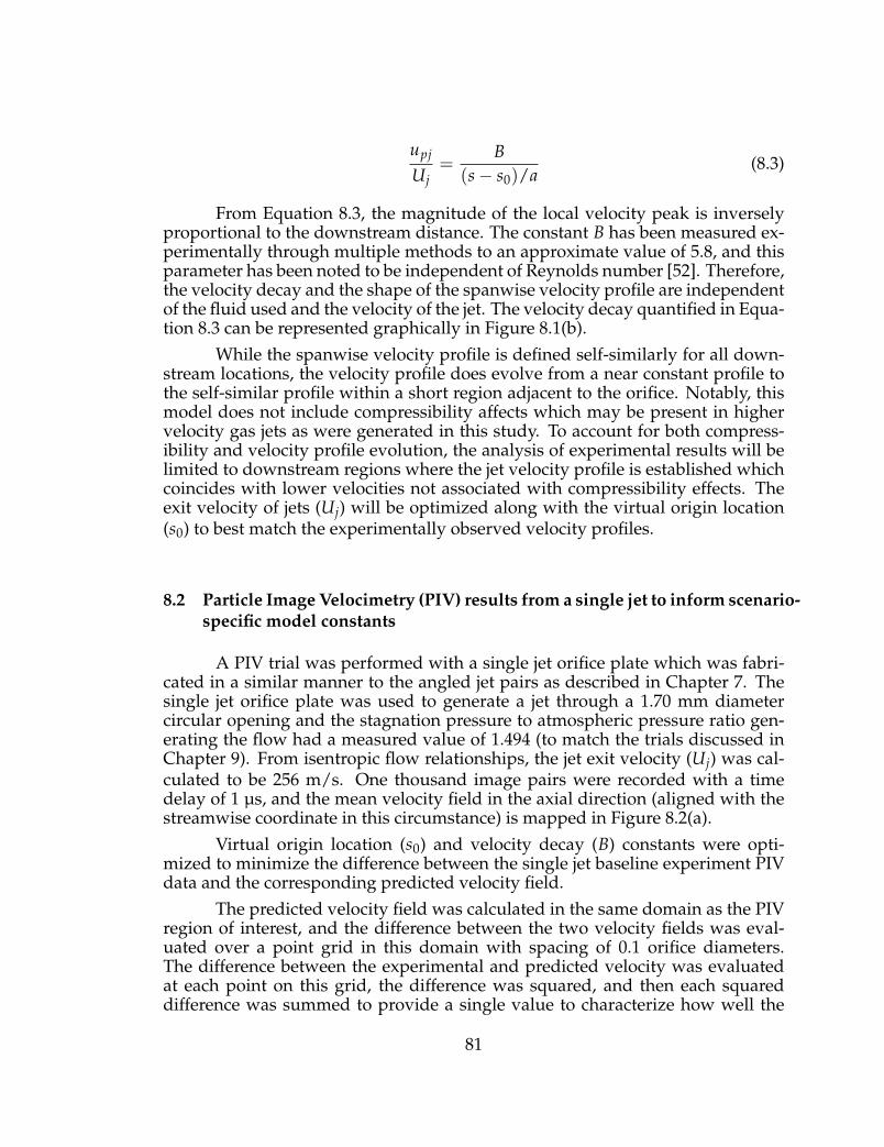
upj

Uj=

B(s− s0)/a

(8.3)

From Equation 8.3, the magnitude of the local velocity peak is inverselyproportional to the downstream distance. The constant B has been measured ex-perimentally through multiple methods to an approximate value of 5.8, and thisparameter has been noted to be independent of Reynolds number [52]. Therefore,the velocity decay and the shape of the spanwise velocity profile are independentof the fluid used and the velocity of the jet. The velocity decay quantified in Equa-tion 8.3 can be represented graphically in Figure 8.1(b).

While the spanwise velocity profile is defined self-similarly for all down-stream locations, the velocity profile does evolve from a near constant profile tothe self-similar profile within a short region adjacent to the orifice. Notably, thismodel does not include compressibility affects which may be present in highervelocity gas jets as were generated in this study. To account for both compress-ibility and velocity profile evolution, the analysis of experimental results will belimited to downstream regions where the jet velocity profile is established whichcoincides with lower velocities not associated with compressibility effects. Theexit velocity of jets (Uj) will be optimized along with the virtual origin location(s0) to best match the experimentally observed velocity profiles.

8.2 Particle Image Velocimetry (PIV) results from a single jet to inform scenario-specific model constants

A PIV trial was performed with a single jet orifice plate which was fabri-cated in a similar manner to the angled jet pairs as described in Chapter 7. Thesingle jet orifice plate was used to generate a jet through a 1.70 mm diametercircular opening and the stagnation pressure to atmospheric pressure ratio gen-erating the flow had a measured value of 1.494 (to match the trials discussed inChapter 9). From isentropic flow relationships, the jet exit velocity (Uj) was cal-culated to be 256 m/s. One thousand image pairs were recorded with a timedelay of 1 µs, and the mean velocity field in the axial direction (aligned with thestreamwise coordinate in this circumstance) is mapped in Figure 8.2(a).

Virtual origin location (s0) and velocity decay (B) constants were opti-mized to minimize the difference between the single jet baseline experiment PIVdata and the corresponding predicted velocity field.

The predicted velocity field was calculated in the same domain as the PIVregion of interest, and the difference between the two velocity fields was eval-uated over a point grid in this domain with spacing of 0.1 orifice diameters.The difference between the experimental and predicted velocity was evaluatedat each point on this grid, the difference was squared, and then each squareddifference was summed to provide a single value to characterize how well the

81

Figure 8.2: (a) Experimental velocity field PIV measurements for a single jet and(b) predicted velocity field for a single jet with optimized model constants.

prediction matched the experimental data. Squaring the velocity difference at in-dividual points was performed to bias the optimization towards matching highervelocity regions of the flow. The virtual origin location (s0/a) and velocity decayconstant (B) were optimized to dimensionless values of 0.89 and 4.70 respectively.As shown in Figure 8.2(b), the predicted flow field contour resembles the mea-sured flow field from Figure 8.2(a). Velocity profiles extracted at various down-stream (x/a) locations in Figure 8.3 show close agreement. The somewhat coun-terintuitive values for these constants, particularly the virtual origin being downstream of the actual jet orifice, is attributed to the varying jet velocity profile andcompressibility effects in the region of the flow closest to the orifice. The highvelocity jet near the orifice retains its velocity better than a jet with a fully selfsimilar velocity profile and does not begin to spread as quickly, which pushes thevirtual origin downstream beyond the jet orifice. The velocity decay constant isslightly lower than the typical value of 5.8.

8.3 Combining multiple single jet profiles to predict multiple jet flow

Here, understanding of the single jet velocity profile as established in lit-erature is utilized to extend basic science understanding of jet flows into a char-acterization of the combined flow and interaction of two, nearby jets. Consider-ing jets without compressibility, interaction ultimately becomes a process wherethe local velocity in the region between the jets must increase to accommodatethe necessary mass flow rate. The multiple jet flow field model developed hereassumes superposition of the velocities from two independently defined jets.For outwardly oriented jets, the geometric parameters which characterize eachunique scenario are the jet spacing (D) and the projection angle between the cen-terlines of the jets (θ). This is schematically represented in Figure 8.4. Parallelinteracting jets are the case if the projection angle is zero which has been studiedin the literature [53] [55]. All coordinate dimensions and the distance between

82

Figure 8.3: A comparison of experimental versus predicted flow at various down-stream distances.

the jet orifices in this section are reported after non-dimensionalization by the jetorifice diameter a is is conventional in the literature [52].

The two main coordinate systems of interest represented in this flow asrepresented in Figure 8.4 are the jet-centric and global axes. The jet-centric axeshave previously been implemented in Section 8.1 which are referred to as stream-wise (s coordinate) and spanwise (r coordinate) where the former is in the direc-tion of the flow. Velocities in the jet-centric coordinate system are given subscriptsof j. The axes in the global coordinate system are referred to as axial (x coordi-nate) and radial (y coordinate) to align with tradition jet flow axes. Velocities inthe global coordinate system are locally referred to as u and v in the axial andradial directions respectively. The jet-centric coordinates are important for defin-ing each jet based on the mean velocity profile presented in the literature, and theglobal coordinates provide a means for evaluating the entire flow and align withthe PIV measurements recorded in experiments.

Since each jet is defined independently when making the total flow fieldprediction, there must be a jet-centric set of axes defined for each jet to define itscontribution to the combined velocity field. Referencing the angled jets issuingroughly from left to right in Figure 8.4, the upper jet will be given the subscript1 while the lower jet will be given subscript 2. To arrive at the upper jet-centriccoordinates from the global coordinates, a vertical transformation of D/2a and acounterclockwise transformation through an angle of θ/2 must be applied. Thistransformation may be written as:

83

Figure 8.4: Annotated two jet flow field schematic with coordinate systems andapplicable velocities.

84

s1 = x cos(

θ

2

)−(

y +D2a

)sin(

θ

2

)r1 = x sin

(θ

2

)+

(y +

D2a

)cos

(θ

2

) (8.4)

Similarly arriving at the lower jet-centric coordinates from the global co-ordinates, requires a vertical transformation of −D/2a and a clockwise transfor-mation through an angle of θ/2. This transformation may be written as:

s2 = x cos(

θ

2

)+

(y− D

2a

)sin(

θ

2

)r2 = −x sin

(θ

2

)+

(y− D

2a

)cos

(θ

2

) (8.5)

From the above coordinate transformations, any location within the globalcoordinate system (x, y) can be rewritten in the local coordinate systems as (s1, r1)or (s2, r2). Using the mean velocity profile discussed in Section 8.1, these twojet-centric locations correspond to local velocities uj,1 and uj,2. These velocitiesremain in the direction of their respective jet.

To combine the flow field into a single flow containing both jets, the ef-fects from jets 1 and 2 are combined via superposition of the velocities uj,1 anduj,2. This approach attempts broadly to approximate conservation of mass by al-lowing the flow from both jets to pass through each point in the flow field, and jetinteraction is manifested as the superposition between the flows. For simplicity,these two values are broken into components aligned with the global coordinatesystem:

u1 = uj,1 cos(

θ

2

)and v1 = uj,1 sin

(θ

2

)(8.6)

u2 = uj,2 cos(

θ

2

)and v2 = −uj,2 sin

(θ

2

)(8.7)

Then the jet specific components u1, v1, u2, and v2, are summed to form the com-bined flow velocity components u in the axial direction and v in the radial direc-tion:

u = u1 + u2 = uj,1 cos(

θ

2

)+ uj,2 cos

(θ

2

)(8.8)

85

v = v1 + v2 = uj,1 sin(

θ

2

)− uj,2 sin

(θ

2

)(8.9)

In summation, the combined flow at any given point of two nearby jets atsome spacing and outward offset angle is calculated by:

1. Defining the point in global coordinates (x, y)

2. Translating the point into both jet-centric coordinate systems as (s1, r1) and(s2, r2)

3. Using Equations 8.1, 8.2, and 8.3 to calculate uj,1 and uj,2

4. Using Equation 8.8 and 8.9 to combine the individual jet contributions intothe axial (u) and radial (v) velocity components of the combined field inglobal coordinates.

8.4 Describing metrics to characterize the intensity of jet interaction in themean velocity field

Jet interactions can be broadly characterized by the velocity in the centerof the combined flow field and the location of the peak velocities when examinedon a line parallel to the radial axis as shown in Figure 8.4. The line parallel to theradial axis can be given the equation x = c and can be evaluated for any constantvalue c > 0. The first characteristic is amplified centerline velocity (uc), and thesecond characteristic is an inward shift of local peak velocity locations. The localpeak velocity (up) is defined as the maximum axial velocity along any given lineparallel to the radial axis. This peak velocity occurs equally at two locations dueto flow field symmetry. Both uc and up are shown in their respective locations inFigure 8.4. The strength of interactions rely on the relative effects of the construc-tive interference of the two jet velocity profiles against their outward orientationand dissipation of the entire flow field as expressed through velocity decay. Thedegree to which jet interactions occur are defined by the offset angle (θ/2) andjet spacing (D/a). Jet interactions are only examined here prior to the axial (x)location where up/U > 0.02. This location corresponds to a local peak axial ve-locity of approximately 1 m/s in the performed PIV experiments. While somesignificant interactions may be predicted at very far distances, these predictionshold little applicability in most practical flows.

The first characteristic of interacting jets is an amplified centerline veloc-ity (uc) due to the superposition of the two jet flows. The centerline velocity ishorizontally directed due to the symmetric nature of the jet arrangement, and isdefined at a radial location of y = 0. While the majority of the flow field deceler-ates as the jets spread and dissipate, the centerline velocity actually increases for

86

some values of x/a along the axial axis before decreasing in the far field. Figure8.5 shows predicted centerline velocity normalized by the axial exit velocity (U)for various jet arrangements.

To characterize relative magnitude of uc to the flow’s cross-section at anyaxial location, the ratio uc/up is implemented. The centerline to local peak ve-locity ratio allows for a simple definition of when jet combination occurs. Jetcombination is the phenomenon which occurs when interaction is so strong thatthere are no longer individual local velocity peaks associated with each of the twooriginal jets. When jets combine, the new combined peak velocity exists along theflow’s axial centerline. As such, jet combination is noted when uc = up, and thiscan be expressed as the ratio uc/up reaching unity.

While some jet pairs are predicted to combine, this only occurs for jets witha small spacing and limited outward projection angle. To describe if the interac-tion between the two jets is relatively significant, a threshold value of uc/up ≥ 0.1is identified. This threshold value was chosen because it reflects the centerlinevelocity reaching a magnitude within one order of magnitude of the local peakvelocity.

The second characteristic of interacting jets is the tendency for the loca-tions (yp) where the local peak velocity (up) occurs to move closer to the centerof the flow rather than maintain trajectories along the streamwise axes. To de-scribe the mechanism behind why the locations of local peak axial velocity arecloser than the streamwise axis trajectory, it is useful to consider the contributionof each jet to the combined flow field individually. Considering a single jet, thelocal peak velocity will always coincide with the jet’s own streamwise axis. Thistrajectory will be maintained throughout the domain. When considering the ve-locity profile of the second jet near the streamwise axis belonging to the first jet,the second jet’s local velocities will always be decreasing away from the secondjets streamwise axis. Therefore, the velocity contribution from the second jet willbe greater on the side of the first jet’s streamwise axis which is closer to the centerof the flow (near the axial axis). As shown in Figure 8.6, this unequal contributionmust shift the peak inwards. The example shown the Figure 8.6 represents signif-icant peak shift, but the shift is more likely less noticeable and even imperceivablein circumstances with large jet offsets.

As previously described, jet combination occurs when two peaks corre-sponding to the individual jets are no longer perceivable (yp = 0). When uc/upreaches unity, the distance from both local peaks to the central axis (yp) simultane-ously reaches zero. This leads to an appearance that the jets are turning towardseach other, but the peak shift and jet merger is truly caused by increasing velocityin the center of the flow due to the velocity superposition. Velocity is directedaway from the center of the flow in all locations except the axial axis.

Using the combined flow field approximation developed in Section 8.3,examples of various scenarios which lead to combination, significant interaction,and no appreciable interaction can be demonstrated. Shown in Figure 8.7, com-bined flow fields were calculated for jets with various offset angles at jet spacings

87

Figure 8.5: (a-c) Centerline velocity versus axial position in combined flow fieldat various spacings and angles.

88

Figure 8.6: Inward shift of peak velocity in combined flow field.

of D/a = 3, 6, and 12. The plots of centerline to local peak velocity ratio ver-sus axial position demonstrate how increased offset angle at a given spacing al-ways leads to a lower predicted interaction. The plots of the location of the localvelocity peak also show how the local velocity peak will pull towards the flowcenterline in higher interaction and combination scenarios, but can often followvery closely to the initial streamwise trajectory. In general, less spacing and angleleads to more interaction and likelihood for combination.

8.5 Outwardly oriented gas jet interaction predictions for fabricated orificeplates

As described in Chapter 7, a series of two jet orifice plates were fabricatedat spacings of D/a = 3, 6, and 12 and at offset angles of θ = 0°, 10°, 20°, 30°, and40 °. To predict the expected interaction intensity along with the possibility of jetcombination, combined flow fields were computed through a range of jet offsetsand separation angles as shown in Figure 8.8, and the location of the fabricatedorifice plates are marked with white stars. The axial location (x/a) where signif-icant interaction (uc/up ≥ 0.1) was first predicted is shown throughout the D/aversus θ parameter space. If the interaction threshold was not reached before thelocal peak velocity diminished to 2% of the axial component of the exit velocity,then no interaction is reported. Additionally, jet combination is predicted to oc-cur on any geometric configuration in the region below the dashed line near thesmallest jet separation and offset values.

89

Figure 8.7: (a, c, e) Centerline to local peak velocity ratio versus axial positionin combined flow field for various jet spacings and offset angles, and (b, d, f)local peak velocity location (solid lines) versus axial position compared to thestreamwise axis trajectory (dashed lines) demonstrating inward peak shift andjet combination.

90

Figure 8.8: Jet interaction map depicting the location of first significant interactionand predicted jet combination region at various combinations of jet spacing andoffset angle.

In Figure 8.8, it is clear that jet interaction should increase with decreasedjet spacing and offset angle. The axial distance needed for significant jet interac-tion to occur increases more rapidly with increasing offset angle than increasingorifice separation. Significant interaction is not predicted to exist at offset anglesabove 23°. Similarly, jet combination appears to only occur at relatively smalloffset angles below 6.8°. In general, jet interactions are predicted to be more sen-sitive to changes in offset angle than spacing.

91

CHAPTER 9

EXPERIMENTAL RESULTS AND DATA ANALYSIS OFSTEADY STATE TWO JET VELOCITY FIELDS

Using the previously described steady state venting apparatus with inter-changeable orifice plates and the Particle Image Velocimetry (PIV) measurementtechnique technique was used to conduct experiments to quantify:

• The velocity field for steady-state gas venting flow from multiple outwardlydirected gas jets.

Time resolved measurements of two jet configurations of various spacingsand offset angles were made to develop a foundational understanding of the jetinteractions.

9.1 Steady state PIV test series

Each individual trial was performed with a unique jet configuration, butthe jet exit velocity was maintained constant throughout the test series. The stag-nation pressure in the upstream stilling chamber was set to 129 kPa for each trial.This gave a stagnation to atmospheric pressure ratio of 1.50. Since the stagnationpressure was not sufficiently large to choke the flow, the jets exited the orificeplate subsonically at atmospheric pressure. The jet exit velocity was calculatedas Mach 0.784 or 256 m/s using isentropic flow relationships. The jets were com-pressible in the region immediately adjacent to the orifice exit. Mean stagna-tion pressure and temperature measurements were recorded during each trial asrecorded in Table 9.1.

One thousand image pairs were recorded during each trial. PIV process-ing in Insight 4G software calculated instantaneous velocity fields as shown inFigure 9.1 for each frame pair. Due to a lack of sufficient environmental particleseeding and high deformation between particle groups, PIV processing reliabilitywas limited in the region nearest the orifice plate. Velocity fields reported herehave been limited to the region beyond 10 diameters from the orifice exit in theaxial direction. By limiting the domain of reported data, non-physical velocitiesassociated with poor PIV correlations have been removed. Additionally, limit-ing the domain of the velocity field analysis limited any complexities associated

92

Table 9.1: Exit velocities for PIV trials calculated from stagnation property mea-surements

Test Stagnation Stagnation Exit Mach Exit velocitygeometry pressure temperature number (Uj)

(kPa, abs) (°C) (m/s)Nominal set point 129 25.0 0.784 256D/a = 3, θ = 0 129 24.2 0.781 255

D/a = 3, θ = 10 129 24.8 0.782 256D/a = 3, θ = 20 129 25.5 0.783 256D/a = 3, θ = 30 129 24.9 0.782 256D/a = 6, θ = 0 128 24.6 0.775 253

D/a = 6, θ = 10 129 24.3 0.784 256D/a = 6, θ = 20 128 23.9 0.778 254D/a = 6, θ = 30 129 24.7 0.783 256D/a = 12, θ = 0 129 25.1 0.780 255

D/a = 12, θ = 10 129 24.8 0.781 255D/a = 12, θ = 20 128 23.7 0.779 254

Test average 129 24.6 0.781 255

with compressibility near the jet exit. Considering the average Mach number of0.781 at the jet exit, u/U values of 0.384, 0.386, 0.390, and 0.398 corresponded tolocal Mach numbers of 0.3 at offset spacings of 0°, 10°, 20°, and 30°respectively.U varies between test geometries as this velocity is in the global axial direction.A Mach number of 0.3 is a typical threshold below which flows are consideredincompressible [67]. Velocities higher than this threshold were only observedand predicted in a small region near the jet local peaks between x/a = 10 andx/a = 12. Limiting the analysis to the incompressible portion of the jet flowallows for better comparison to the predicted flow model which is based on pre-vious experimentation on incompressible jets.

The instantaneous velocity fields were used to calculate mean velocity andturbulence statistics. Since the flow was sufficiently fast compared to the 84.9 mmPIV field of view and 15 Hz laser repetition rate, individual turbulent structurescould not be tracked between successive frame pairs.

93

Figure 9.1: (a-d) Still frames recorded during a PIV trial which were processed tocreate (e, f) instantaneous velocity fields.

94

9.2 Mean velocity field measurements

Instantaneous velocity field measurements were used to calculate the meanvelocity field for each two jet geometry tested. Figures 9.2 through 9.6 show axialvelocity distributions throughout the measured flow field as contour plots for theD/a = 3, D/a = 6, and D/a = 12 geometries at various angles (θ), respectively.These contours are compared against the predicted velocity field calculated fromthe method described in Chapter 8. In all contour plots, the axial component ofthe mean velocity (u) is normalized by the axial component (U) of the jet exitvelocity (Uj).

Jets pairs with the closest spacings and offset angles typically demon-strated more interaction than those with either a wider spacing or offset angle.The analytical model prediction and experimental results flow field characteris-tics compared well in all trials. In all three spacings, the parallel jets tended topull together towards combining into a single velocity profile. Within the experi-mental region of interest, the 3 and 6 diameter cases did combine such that therewas only a single resolved velocity peak. Jet combination in these two cases alsoled to higher retained velocity for further distances in the axial direction. Jets withoffset angles of 10° consistently demonstrated the highest mean velocities in theregion between the two jets, but less interaction was present for the D/a = 12,θ = 10 trial. Much less interaction was predicted and observed at angles of 20°or 30°.

In addition to the velocities, radial cross sections of the mean axial veloc-ity field were plotted at various axial (x/a) locations as shown in Figures 9.8, 9.9,and 9.10. The predicted flow and experimental results captured the same velocityprofile trends in all cases. The differences between predicted and experimentalvelocity profiles were similar to the precision of the optimized single jet profilein Chapter 8. Initially, all flow fields showed two distinct velocity peaks associ-ated with each individual jet. All velocity profiles decayed and spread at crosssections further downstream. In cases with little or no interaction, the individualjet profiles closely resemble single jets, and jet peaks moved away from the flowfield centerline.

When interaction between the two jets was observed, the outer side of eachjet velocity profile appeared relatively unaffected. However, the constructive in-terference of the two jets near the center of the flow caused increasing centerlinevelocities downstream and less steep velocity gradients in the area near the centerof the flow. Though less steep than the outside of the jet, the velocity profile fromeither jet’s local peak to the centerline velocity qualitatively appeared similar tothe Gaussian-like profile of a single jet.

Parallel jets which combined into a single profile, or likely would haveif measurements extended further downstream, demonstrated interaction in themean velocity profile similar to angled jets. Combination occurred rapidly afterthe centerline velocity was similar to the peak velocity such as the x/a = 25or x/a = 35 profiles for the 3 and 6 diameter spacing trials, respectively. Thevelocity profile between the two peaks began to level after these profiles, and the

95

Figure 9.2: Contour plot comparison between (a and c) experimentally recordedand (b and d) predicted mean velocity fields for jets with an orifice spacing orD/a = 3 and offset angles of 0°and 10°.

96

Figure 9.3: Contour plot comparison between (a and c) experimentally recordedand (b and d) predicted mean velocity fields for jets with an orifice spacing orD/a = 3 and offset angles of 20°and 30°.

97

Figure 9.4: Contour plot comparison between (a and c) experimentally recordedand (b and d) predicted mean velocity fields for jets with an orifice spacing orD/a = 6 and offset angles of 0°and 10°.

98

Figure 9.5: Contour plot comparison between (a and c) experimentally recordedand (b and d) predicted mean velocity fields for jets with an orifice spacing orD/a = 6 and offset angles of 20°and 30°.

99

Figure 9.6: Contour plot comparison between (a, c, e, g) experimentally recordedand (b, d, f, h) predicted mean velocity fields for jets with an orifice spacing orD/a = 12 and offset angles of 0°, 10°, and 20°.

100

velocity peaks rapidly pulled to the center of the flow field. After jet combination,only a single velocity peak was able to be resolved.

In some trials, the relative strength of the two jets appeared uneven thoughthe predicted velocity field is symmetric. An example of this is the D/a = 6,θ = 20 trial. This is attributed to a slight imprecision in the alignment of theorifice plate during mounting. The clearance between the mounting screws andtheir associated holes in the orifice plates allowed for a small rotation of the plate.As such, the laser sheet did not illuminate the exact center of either jet causingthe measured velocities to be lower than expected.

Various uncertainty quantification methods have been developed and com-pared for evaluating PIV datasets, and more sophisticated methods have incor-porated evaluation of cross correlation performance [96, 97]. Here, a conservativeuncertainty propagation is implemented which relies on calculating mean axialvelocity uncertainty (Uu) as:

Uu =σu(t)√

N(9.1)

where σu(t) is the standard deviation of instantaneous velocity measure-ments (u(t)) and N is the number of frame pairs recorded (N = 1, 000 for alltests here) [98]. By using the standard deviation of instantaneous velocity mea-surements, this method accounts for, but does not differentiate between, uncer-tainty associated with the actual turbulent nature of the measurement and mea-surement errors in data collection and processing [98]. Since axial velocity is afunction of the position within the field of view, velocity uncertainty is variablethroughout the measurement domain. This is represented for the D/a = 6 andθ = 0 trial in Figure 9.7. Of note, mean axial velocity uncertainty calculatedsimilarly to and is directly proportional to the turbulence strength discussedin Section 9.3. Spatial trends in mean velocity uncertainty can thus be inferredfrom Figures 9.13 through 9.15. The maximum mean axial velocity uncertaintyrecorded from all trials was 2 m/s which occurred near the orifices of the jets forthe D/a = 6, θ = 0 trial. This is a conservative estimation for uncertainty inthe region of the flow near the jet orifices at axial distances below approximatelyx/a = 10. Mean axial velocity uncertainty further downstream is below approx-imately 0.7 m/s.

101

Figure 9.7: Local mean axial velocity uncertainty contour for the D/a = 6, θ = 0

trial which has the largest uncertainty value observed here.

9.2.1 Centerline velocity changes in the axial direction

The ratio of centerline velocity to the local peak velocity (uc/up) can be aquantification for describing the level of interaction between two jets at some ax-ial location (x/a). Shown in Figure 9.11, the centerline to local peak velocity ratioincreases throughout the PIV measurement region of interest. This ratio reachedunity for the 3 and 6 diameter parallel jet cases as these jets were observed tocombine prior to 50 diameters downstream in the axial direction. Additionally,all 10° jets and the D/a = 3, θ = 20 trials showed significant interaction aspreviously defined of the uc/up ratio reaching a value of 0.1. It is likely that theD/a = 6, θ = 20 trial would have also interacted before the flow dissipated, butthe maximum uc/up value observed within the measurement domain was 0.066.The remaining trials showed little increase in centerline velocity, so the jets didnot interact.

In all test geometries represented in Figure 9.11, the PIV results showedinteraction occurring before the predicted flow field. This was particularly ap-parent at the smallest spacings and offset angles and in the region of the flowfield closest to the jet orifices. This is likely related to the prediction underesti-mating the width of the jets at given locations, because the prediction and PIVmeasurements both showed uc/up ratios tenting towards similar values furtherin the flow field.

102

Figure 9.8: Axial velocity profile comparison between PIV measurements andmodel predictions at various axial locations for jets with orifice spacing of D/a =3.

103

Figure 9.9: Axial velocity profile comparison between PIV measurements andmodel predictions at various axial locations for jets with orifice spacing of D/a =6.

104

Figure 9.10: Axial velocity profile comparison between PIV measurements andmodel predictions at various axial locations for jets with orifice spacing of D/a =12.

105

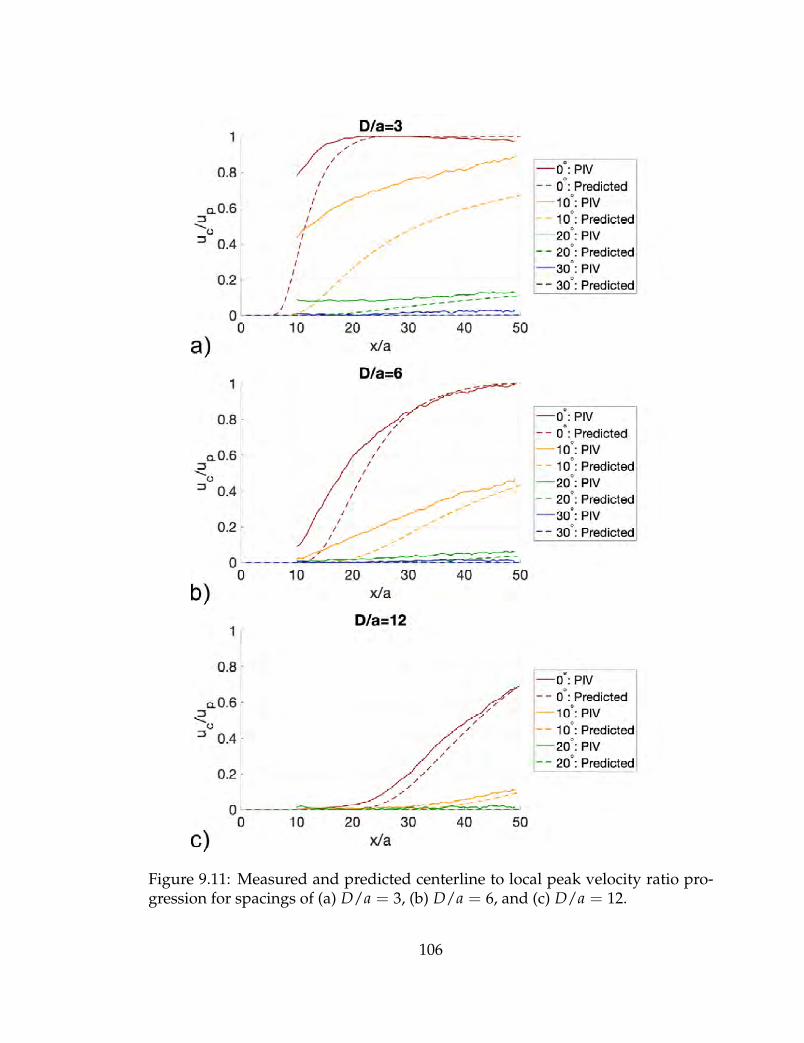
Figure 9.11: Measured and predicted centerline to local peak velocity ratio pro-gression for spacings of (a) D/a = 3, (b) D/a = 6, and (c) D/a = 12.

106

9.2.2 Tracking local peak velocity in the mean flow field

During the discussion of the predicted two jet flow field, an inward shiftin local peak velocity associated with the superposition of the two jets’ contri-butions to the combined field was discussed. The observed location of the localpeak velocities associated with the top and bottom jets was tracked throughoutthe PIV region of interest and compared to the predicted flow field in Figure 9.12.Top and bottom jet nomenclature refers to the location of the jet in the positive ornegative y/a half of the PIV region of interest respectively as visualized in Figures9.2(a and c), 9.3(a and c), 9.4(a and c), 9.5(a and c), and 9.6(a, c, and e). Generally,prediction captured the progression of the local peak velocity locations well in-cluding the distinct, inward curving path for the parallel jets. The accuracy of theprediction was greater for narrower jets. The inaccuracies at the 30° offset angletrials were likely associated with orifice plate machining imprecision particularlyregarding the internal and external surface qualities of the orifice plates.

107

Figure 9.12: Measured and predicted local peak velocity location progression forspacings of (a) D/a = 3, (b) D/a = 6, and (c) D/a = 12.

108

9.3 Turbulence strength observations

Turbulence strength fields were calculated for each of the trials in thistest series as another method to characterize the jet interactions. The turbulencestrength is calculated as the root-mean-square of the turbulent velocity and isused to describe much turbulence varies the velocity at a given location from themean flow. Turbulent velocity (u′(t)) is calculated as the difference between theinstantaneous velocity (u(t)) at some point and the corresponding mean velocity(u) at that location as:

u′(t) = u(t)− u (9.2)

Turbulent strength (u′rms) was calculated for each point in the flow field as:

u′rms =

√√√√ 1N

N

∑n=1

[u′(tn)]2 (9.3)

where N represents the number of PIV frame pairs in the dataset. Likemean velocity previously reported, turbulent strength calculations are reportedhere focus on the axial component of the flow and were normalized by the axialcomponent of the jet exit velocity (U).

Figures 9.13, 9.14, and 9.15 show the contour maps and radial cross sec-tions of the turbulent strength fields for each of the trials at 3, 6, and 12 diameterspacings respectively. Jet pairs with smaller spacings and offset angles had in-creased levels of turbulence in the region between the two jets than the outerperiphery of the flow. The jet pairs with the highest levels of interaction basedon the mean velocity field also had the most notable increase in turbulence in thecentral region of the flow.

In all scenarios, the turbulence cross sections initially captured two mainpeaks associated with the each jet in the pair. Smaller local peaks were associ-ated with the maximum shear stress in each jet, and the local mean peak velocitycoincided with the valley in the middle of these two locations. These profilesdecayed, spread, and appeared to constructively interfere similarly to the meanvelocity profiles in Section 9.2. The turbulence strength profiles began to combineinto a single profile where the initial effects of either jet were no longer able to beresolved similar to the mean velocity field measurements. However, unlike themean velocity field which combined and resembled a single jet, the combined tur-bulence fields resemble a broad plateau of fairly consistent turbulence strength.Additionally, turbulence combination was seen before jet combination and evenin scenarios such as D/a = 3, θ = 10 where jet combination was not predictedbefore the jets were dissipated (per Figure 8.8). In scenarios where the turbulencestrength profiles did not fully combine, the turbulence profiles became largelybroad plateaus with only small peaks associated with the initial jet profiles and asmall valley along the flow centerline. Generally, the turbulence strength profiles

109

follow demonstrated greatest interaction at closely spaced and narrowly offset orparallel jet configurations, and the distinction in the turbulence profile betweenthe two jets became minimal relatively early in the flow field.

110

Figure 9.13: (a, c, e, g) Turbulence strength contours and (b, d, f, h) profiles forPIV trials with orifice spacing of D/a = 3.

111

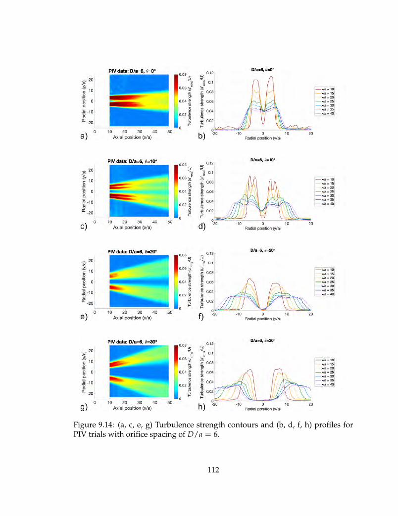
Figure 9.14: (a, c, e, g) Turbulence strength contours and (b, d, f, h) profiles forPIV trials with orifice spacing of D/a = 6.

112

Figure 9.15: (a, c, e) Turbulence strength contours and (b, d, f) profiles for PIVtrials with orifice spacing of D/a = 12.

113

9.4 Estimated mass flow entrainment from experimentally observed flow fields

9.4.1 Estimating three-dimensional flow field from two-dimensionalPIV data

To describe how mass flow was entrained as jet flows evolved in the globalaxial (x) direction, mass flow rate m is defined as:

m = ρ∫

udA (9.4)

where the jets were evaluated as incompressible such that trends in mass flowrate were solely attributed to changes in the velocity field. Additionally, the axialvelocity component u was used, and the surface through which the integral wasevaluated (dA) was perpendicular to this velocity component. A limitation to theability to directly quantify mass flow rate from the experiments performed hereis the two-dimensional nature of the PIV data recorded while information aboutthe full three-dimensional velocity fields was required to evaluate the integral inEquation 9.4. Accordingly, assumptions were made to expand PIV measurementsinto approximated three-dimensional velocity fields to complete the mass flowrate calculation.

A typical and logical assumption for jet flows would be assuming radialsymmetry and reforming Equation 9.4 in cylindrical coordinates. Shown in Fig-ure 9.16, performing this calculation on the baseline single jet experiment cap-tured the linear mass flow entrainment trend as the mean velocity profile modeldescribed in Section 8.1. Entrainment rate here refers to the rate of change of thequantified mass flow rate in Equation 9.4 with respect to changes in axial posi-tion. The mass flow rate calculation based on the mean velocity profile model ispredicted to be inaccurate at values of x/a < 10 due to compressibility effectsand the downstream location of the virtual origin. Offset in the slopes of theselines was attributed to different jet velocity profile shapes as reported in Figure8.3. Reported mass flow rates have been normalized by the flow rate at the orificeplate as calculated from isentropic flow relations and stagnation property mea-surements. The predicted flow field had a wider jet profile than the PIV datawhich caused an increase in the mass flow rate integral. Jet prediction modelconstants optimization was biased to capture local velocity peaks rather than thelower velocity tails of the jet profile which comprised the majority of the massflow rate. Assuming radial symmetry captured the entrainment characteristics ofa single jet. However, a radial symmetry approximation does not work for thetwo jet configurations as these flows were not rotationally symmetric.

From observations reported in literature on rows of parallel jets at variousspacings, the velocity profile in the out-of-plane direction (not measured here) isself similar to the single jet profile [99]. It is assumed that this observation wouldextend to outwardly angled jets as the flow field similarities between parallel andangled jets have been demonstrated here. Here, the third axis to complete the full

114

Figure 9.16: Comparing predicted mass flow rate from the single jet velocity fieldmodel to approximations based on the measured PIV velocity field.

flow field is referred to as “out-of-PIV-plane” and its coordinate location is giventhe variable z. The local peak to the jet profile in the out-of-PIV-plane directionoccurs at z = 0 in the xy-plane which contains both orifices and the trajectory ofeach jet. Since the PIV data recorded here was taken in this xy-plane, the mea-sured velocity fields reported in Figures 9.2 through 9.6 were used as the basisto estimate the entire three-dimensional flow field. Shown in Figure 9.17(a) and(b), the full three-dimensional velocity field of a flow was reconstructed by us-ing rows of data from the PIV measured xy-plane to approximate the remainderof the yz-plane velocity field at various axial (x/a) positions. Within an approx-imated yz-plane velocity field, the only directly measured data was at z = 0.Moving away from the data at z = 0, the approximated local velocities followa jet profile (represented in Figure 9.17(c)) which is defined for each radial po-sition (y/a) in the plane. Advantages of this flow field approximation methodinclude the ability account for the interacting region between jets and no needfor prior knowledge about the flow field such as an axis of symmetry or any jetconfiguration geometry. Additionally, mass flow rate can be easily calculated bynumerically integrating the approximated yz-plane velocity fields at any axiallocation.

This flow field reconstruction technique was also compared to the massflow rate entrainment estimation calculated from the mean velocity profile modelin Figure 9.16. Similar to the model prediction and the previous rotational sym-metry calculation, mass flow rate increased linearly with axial position. The slopediscrepancy between assuming the z-direction profile and the model was smallerthan when rotational symmetry was evaluated because the jet profile in the as-sumed z-direction technique matched the shape of the model more closely. Sincethe three-dimensional flow field constructed by assuming a jet velocity profile inthe z-direction captures similar mass flow rate trends to model prediction and

115

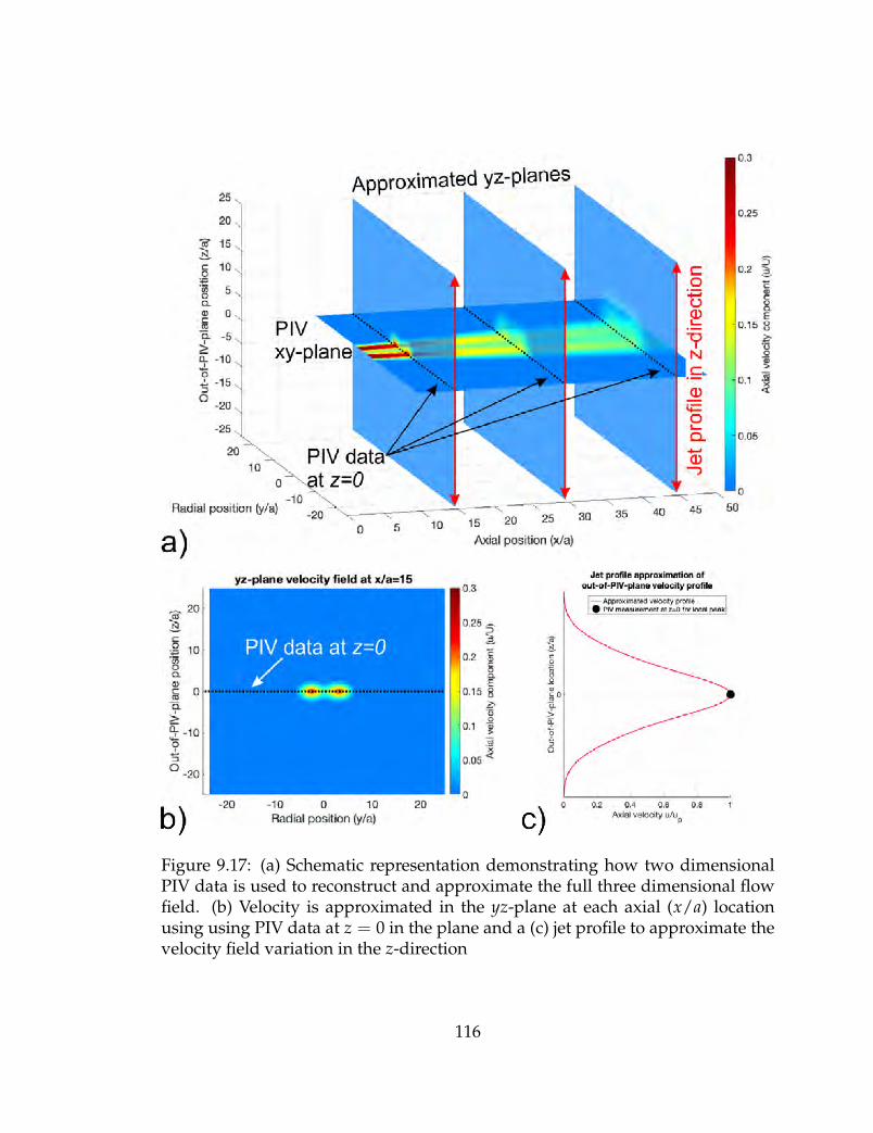
Figure 9.17: (a) Schematic representation demonstrating how two dimensionalPIV data is used to reconstruct and approximate the full three dimensional flowfield. (b) Velocity is approximated in the yz-plane at each axial (x/a) locationusing using PIV data at z = 0 in the plane and a (c) jet profile to approximate thevelocity field variation in the z-direction

116

the typical rotational symmetry argument for a single jet, this method was usedto evaluate mass flow rate for the two jet configurations.

9.4.2 Mass flow entrainment observations for pairs of outwardly an-gled jet pairs

Using the three-dimensional flow field reconstruction method which as-sumes a jet profile in the out-of-PIV-plane z-direction, mass flow rate was cal-culated versus axial position for the parallel and angled jet pairs at normalizedorifice spacings of D/a = 3 and D/a = 6. The D/a = 12 trials were excludedfrom this analysis because their spacing resulted in clipping of the flow field atthe edge of the PIV field of view. Further, due to the superposition method formodeling of the two jet configurations, mass flow rate entrainment was predictedto be equal for all test geometries. For this reason, this analysis focuses on the re-sults obtained through the approximated three-dimensional flow fields generatedfrom experimental data.

Shown in Figure 9.18, all jet configurations demonstrated an increasingmass flow rate as a function of axial position as the jet pairs spread and interactedwith each other. Here, mass flow rate is reported as a ratio of the mass flow rateestimated at a specific x/a location to the mass flow rate at the orifice plate whichwas calculated from stagnation properties. The outwardly oriented jet pairs of allangles demonstrated similar, consistent entrainment rates throughout the regionof interest.

The D/a = 6, θ = 10 example has a higher than typical mass flow rateassociated with relatively higher and more symmetric jet velocity profiles thanthe θ = 20 and θ = 30 examples which can be observed in Figure 9.9. Thisexample still demonstrated a similar mass entrainment rate to the other angledjet configurations which was noted by the slope of the mass flow rate trend. Todemonstrate the similarity in entrainment rates between trials without the offsetseen in the D/a = 6, θ = 10 example in Figure 9.18, the mass flow rate trendswere re-normalized by the observed flow rate at x/a = 10 at the beginning of thePIV quantification region as shown in Figure 9.18. In these plots, the angled jetsmass flow rate trends more closely coalesced along a consistent entrainment rate.

While angled jets appeared to demonstrate similar mass flow rate changesas a function of axial position, the parallel jets scenarios showed an entrainmentrate which decreased at further locations. Particularly noticeable in the D/a = 6parallel jet example, the mass flow rate trend compared similarly to the angledjets at first, but significant divergence was noted after approximately x/a = 25.This divergence occurred while interaction between the two jets was significantas demonstrated with a uc/up ratio of nearly 0.75. Similar interaction was ob-served earlier in the parallel D/a = 3 trial which was likely the cause of themass flow rate divergence from the angled jet cases sooner in the axial direction.These observations were also made by E. B. Gordon and I. Greber for experi-ments on rows of parallel jets where mass flow rate increased similarly for all jet

117

Figure 9.18: Mass flow rate versus axial position approximated from PIV mea-sured velocity fields for the (a) D/a = 3 and (b) D/a = 6 test geometries. Massflow rate is normalized by the flow rate at the jet orifices as determined fromstagnation pressure and temperature.

Figure 9.19: Mass flow rate versus axial position approximated from PIV mea-sured velocity fields for the (a) D/a = 3 and (b) D/a = 6 test geometries. Massflow rate is normalized by the flow rate at the x/a = 10 flow cross section tominimize vertical deviations between tests.

118

spacings for some distance downstream until entrainment rate slowed [99]. Thelocation where entrainment rate began to slow increased with increasing initialorifice spacing. Here, an outward offset angle had a similar effect to increasedorifice spacing because both of these geometric changes minimized the interac-tion between jets thus allowing each individual jet more space to freely spreadand, importantly, interact with and ultimately entrain fluid from the quiescentenvironment. Since it was observed that increased offset angle has a more promi-nent effect on minimizing the intensity of jet interactions than increased orificespacing, variations in entrainment rate were only observed in the trials withoutany outward jet orientation.

119

CHAPTER 10

CONCLUSIONS

The battery venting process under abuse conditions was investigated bydeveloping a new technique for pre-burst pressure measurement and character-izations of the subsequent venting flow. The implementation of case strain wasunique among battery abuse experiments. The optical flow measurements pro-vided a more thorough characterization of the fluid dynamics of battery ventingthan previously attained. A greater scientific knowledge of lithium ion batterysafety was developed as the physical mechanism contributing to their greatesthazards has been uniquely characterized.

The body of work presented here provides unique and useful quantifica-tions and deeper understanding of the dynamics of pressure driven venting flowscomprised of multiple jets into a quiescent environment. While an application ofinterest during these experiments was lithium ion battery venting failures, themethods and analysis performed here were conducted such that the findings arenot limited to this specific application.

10.1 General remarks on non-invasive pressure monitoring and the subse-quent venting dynamics

A methodology for strain based internal pressure measurement on boththin and thick walled cylinders was developed. A test apparatus was constructedallowing the non-invasive measurement of pressure build up during heating of atest specimen. Validation experiments were performed which demonstrated thecapabilities and repeatability of the developed experimental method. Repeatedtrials measured the predictable pressure response of carbon dioxide in a sealedcylinder during constant volume heating.

High speed schlieren imaging measured transient single-phase and multi-phase venting into the environment immediately after burst and its evolutionwith time. Two different concentrations of sucrose solutions were tested andexhibited different droplet breakup regimes. The lower viscosity solution wasatomized while the higher viscosity solution exhibited a second wind-inducedbreakup regime. Droplet spray angle was initially much wider than gas jet spread-ing and tended to zero as the liquid was expelled, but gas projection and spread-ing was consistent throughout the simulated burst event. The low viscosity, at-

120

omized flow was wider than the high viscosity, wind-blown spray. The outeredges of multiphase transient venting flow was initially populated with particlesbut was eventually bounded by gas. Since initial droplet spray angle was, widerthan the offset angle between the jets in the vent cap tested, nearby multiphaseventing flow characterization should consider spray interactions between jets inthe entire combined flow field.

Tip penetration and time-of-arrival measurements demonstrated that theinclusion of liquid decreases the rate of flow front penetration into the environ-ment. The flow front of small atomized particles from the low viscosity sucrosesolution were much closer to matching the gas-only trial than the high viscosity,wind-induced flow. While the high viscosity droplets were slower, they deceler-ate less quickly than the gas or atomized droplets which may lead to greater totalpenetration into the surroundings.

The combined flow field from two nearby, outwardly angled jets was in-vestigated in order to increase the basic, scientific understanding of jet interac-tions common in venting scenarios. To predict how jet interactions would occur,a simple model based on superposition of a single jet velocity profile was devel-oped to make a priori predictions of the combined mean velocity field createdby the two nearby jets. Model constants were optimized for the specific orificeshape and testing conditions by optimizing velocity decay and virtual origin lo-cation for a single jet baseline experiment. This model was used to develop usefulmetrics and predict the range of spacings and offset angles where jet combinationor significant interaction was expected to occur. By predicting the combined flowfor a broad range of angled jet geometries, it was observed that the strength ofjet interactions is more easily diminished by increasing offset angle rather thanorifice spacing. In contrast, jets with significantly large spacing or offset anglelarger than approximately 23° may be considered independent.

PIV experiments were performed at jet orifice spacings of 3, 6, and 12 di-ameters with offset angles of 0°, 10°, 20°, and 30°. Velocity profiles from PIVmeasurements compared similarly to model predictions. The intensity of jet in-teraction was quantified by both following the evolution of the centerline veloc-ity between the jets as a percentage of the local peak velocity along with trackingthe inward shift of the local peak velocity caused by the superposition of the jetflows. Mean axial velocity measurements demonstrated increased interaction be-tween the jets at smaller offset angles and closer orifice spacings. Combinationof the jets was observed for parallel jet examples at 3 and 6 diameter orifice spac-ings. As predicted by the model, interaction between the two jets appeared moresensitive to changes in offset angle than initial spacing. Similar to the mean ve-locity profiles, turbulence was amplified in the region between the two jets, andincreased turbulence was noticed closer to the orifices in the flow field than in-creases in mean velocity. An approximation of mass flow entrainment was devel-oped from the recorded PIV velocity fields which demonstrated that mass flowrate increased with further axial distance from jet orifices. The two jet geome-tries which combined in the PIV field of view demonstrated relatively decreasedentrainment at downstream axial positions.

121

10.2 Findings specific to lithium ion battery safety

Using the non-invasive pressure measurement methodology, a series ofexperiments on live 18650 format batteries was performed at heating rates of2.4°C/min, 3.6°C/min, and 4.8°C/min. The highest rate test was performed induplicate. All tests captured a final pressure rise before venting onset beginningbetween battery surface temperatures of 138°C and 151°C. The observed finalpressure rise in all trials had magnitudes comparable to the known burst pres-sure of the vent caps installed on the brand of battery tested. The rate of pressurebuild up within each battery increased before venting onset. By examining sur-face temperature measurements made throughout these abuse experiments, itwas observed that the internal pressure build up before venting corresponds tothe onset of battery self-heating which indicates thermal runaway. Erroneous in-dicated internal pressure measurements before the final pressure build up wereattributed to interactions between internal battery components and the case in-cluding the possibility of localized component failures within the cell.

The novel ability to monitor the final pressure rise indicative of an im-minent venting failure provides a useful, noninvasive diagnostic technique forbattery abuse testing. However, battery self heating was also observed as an in-dicator of imminent venting failure. Temperature measurement was more simpleto implement than strain regarding the complexity of the experimental hardware,data acquisition needs, and data processing. Strain measurement corrections re-lied on knowing the battery case temperature throughout each trial, so straincan only be realistically implemented in conjunction with temperature measure-ments. Strain based internal pressure measurement was effective for observingthermal runaway and gas generation prior to venting onset, but this methodshould not be considered a replacement for temperature measurement as a meansof state-of-health monitoring.

Venting experiments performed here demonstrated that gas jet pairs showincreased interaction at low orifice spacings and offset angles. Given the approx-imate orifice spacing of D/a = 6 for an 18650 format battery and an observed off-set angle of 42°, the significantly wide offset angle would prevent any significantjet interactions from occurring even at this moderate diameter spacing. Gas vent-ing from a typical 18650 format battery may be considered as four independentjets. However, the initial droplet spray cone angle of 97° and the significant con-centration of atomized particles during the low viscosity sucrose solution bursttest indicates that spray patterns within the entire droplet field must be consid-ered as a whole to characterize multiphase battery venting.

10.3 Future work

One main limitation to the strain based internal pressure build up mea-surement methodology developed here is the potential for interactions between

122

the tightly wound electrochemical components and the outer case of a cylindri-cal battery causing erroneous strain measurements. Refocusing investigation onmore deformable battery construction styles, such as pouch cells, may be an alter-native path to studying gas generation throughout the thermal runaway process.Pouch style batteries typically swell during failure. Methods could be developedto correlate the deformation of an unconstrained cell to internal pressure. Alter-natively, these cells could be constrained during failure, and the load exerted byon a hypothetical test fixture would correspond to the gas generation within thebattery. By advancing the understanding of pressure build up in cells of differentconstruction but identical chemistries, inferences could be made on the internalstate of cylindrical cells during thermal runaway.

Future investigation into the interaction of nearby gas jets can advanceunderstanding of venting flows in multiple useful ways. An important investi-gation would be evaluating the accuracy and limitations of the velocity super-position modeling method in other configurations such as inwardly angled jetsor flows caused by more than two equal strength jets. Superposition of otherflow properties which have been characterized for single jets, such as turbulencestrength, may yield useful predictions as well. Another consideration for eval-uating the hazards of venting flows, including from failing batteries, is the sur-rounding into which venting occurs. Here the environment adjacent the ventingflow was both quiescent and unobstructed, but many real-world scenarios mayinclude unrelated flows (e.g. heating, ventilation, and air conditioning) and ad-ditional structures or enclosures. Investigating the effect of atmospheric pressureon multiple jet flow interaction may also be of interest for aviation or space flightapplications. The presence of unique complexities would alter characteristics ofventing flows.

Additional research should be performed to quantify flammability of tran-sient, multiphase venting. Both gas mixing and droplet spray will have importantcontributions to the overall combustibility of flammable vented material. Theseexperiments should be complimented by further testing on live batteries to quan-tify parameters such as droplet size and velocity to understand propagation intothe environment.

123

BIBLIOGRAPHY

[1] H. J. Hussein, S. P. Capp, and W. K. George. Velocity measurements in ahigh-reynolds-number, momentum-conserving, axisymmetric, turbulent jet.Journal of Fluid Mechanics, 258:31–75, 1994.

[2] B. Scrosati and J. Garche. Lithium batteries: Status, prospects and future.Journal of Power Sources, 195:2419–2430, 2010.

[3] J. Boyes and I. Gyuk. Electrical energy storage for utility scale applications.In Electric Power, 2007.

[4] K. Lynn et al. US battery storage market trends. Technical report, EnergyInformation Administration, 2018.

[5] C. Kang. Galaxy Note 7 owners are urged to stop using their phones. NewYork Times, 9 September 2016.

[6] U. Irfan. How lithium ion batteries grounded the Dreamliner: Official reporton Boeing 787 fires tells a cautionary tale about advanced batteries. ScientificAmerican, 18 December 2014.

[7] S Abada et al. Safety focused modeling of lithium-ion batteries: A review.Journal of Power Sources, 306:178–192, 2016.

[8] L. A. McKenna. Electronic cigarette fires and explosions in the United States2009 - 2016. Technical report, FEMA, 2017.

[9] F. A. Mier. Measurement of 18650 format lithium ion battery vent mecha-nism flow parameters. Masters Thesis, 2018.

[10] V. Muenzel et al. A comparative testing study of commercial 18650-formatlithium-ion battery cells. Journal of The Electrochemical Society, 162(8):A1592–A1600, May 2015.

[11] Phillip Weicker. A Systems Approach to Lithium-Ion Battery Management.Artech House, 2014.

[12] Q. Wang et al. Thermal runaway caused fire and explosion of lithium ionbattery. Journal of Power Sources, 208:210:224, 2012.

[13] E. P. Roth et al. Advanced technology development program for lithium-ionbatteries: Thermal abuse performance of 18650 li-ion cells. Technical ReportSAND2004-0584, Sandia National Laboratories, 2004.

124

[14] S. S. Zhang. Insight into the gassing problem of Li-ion battery. Frontiers inEnergy Research, 2:1–4, 2014.

[15] C. Mikolajczak et al. Lithium-Ion Batteries Hazard and Use Assessment.Springer, 2011.

[16] MTI Corp. 18650 cylinder cell case with anti-explosive cap and insulationo-ring - 100 pcs/package - eq-lib-18650, 2013.

[17] Engineering and safety center technical bulletin. Technical Report No. 09-02,NASA, 2009.

[18] P. G. Balakrishnan, R. Ramesh, and T. Prem Kumar. Safety mechanisms inlithium-ion batteries. Journal of Power Sources, 155:401–414, 2006.

[19] T. Unkelhaeuser and D. Smallwood. United States Advanced Battery Con-sortium electrochemical storage system abuse test procedure manual. Tech-nical Report SAND99-0497, Sandia National Laboratories, 1999.

[20] W. C. Chen et al. Effects of thermal hazard on 18650 lithium-ion batteryunder different states of charge. J Therm Anal Calorim, 121:525–531, 2015.

[21] R. E. Lyon and R. N. Walters. Energetics of lithium ion battery failure. Journalof Hazardous Materials, 318:164–172, 2016.

[22] Y Fu et al. An experimental study on burning behaviors of 18650 lithiumion batteries using a cone calorimeter. Journal of Power Sources, 273:216–222,2015.

[23] D. P. Finegan et al. In-operando high-speed tomography of lithium-ion bat-teries during thermal runaway. Nature Communications, 2015.

[24] J. Lamb and C. J. Orendorff. Evaluation of mechanical abuse techniques inlithium ion batteries. Journal of Power Sources, 247:189–196, 2014.

[25] H. Wang et al. Mechanical abuse simulation and thermal runaway risks oflarge- format Li-ion batteries. Journal of Power Sources, 342:913–920, 2017.

[26] H. Huang et al. Lithium metal phosphates, power and automotive applica-tions. Journal of Power Sources, 189:748–751, 2009.

[27] X. Liu et al. Heat release during thermally-induced failure of a lithium ionbattery: Impact of cathode composition. Fire Safety Journal, 85:10–22, 2016.

[28] A. W. Golubkov et al. Thermal-runaway experiments on consumer Li-ionbatteries with metal-oxide and olivin-type cathodes. RSC Advances, 4:3633–3642, 2014.

[29] Q. Wang et al. Combustion behavior of lithium iron phosphate battery in-duced by external heat radiation. Journal of Loss Prevention in the ProcessIndustries, 49:961–969, 2017.

125

[30] F. Larsson et al. Characteristics of lithium-ion batteries during fire tests.Journal of Power Sources, 271:414–420, 2014.

[31] B. L. Ellis et al. A multifunctional 3.5 V iron-based phosphate cathode forrechargeable batteries. Nature Materials, 6:749–753, 2007.

[32] P. Ping et al. Study of the fire behavior of high-energy lithium-ion batterieswith full-scale burning test. Journal of Power Sources, 285:80–89, 2015.

[33] N. S. Spinner et al. Physical and chemical analysis of lithium-ion batterycell-to-cell failure events inside custom fire chamber. Journal of Power Sources,279:713–721, 2015.

[34] P. T. Coman et al. Numerical analysis of heat propagation in a battery packusing a novel technology for triggering thermal runaway. Applied Energy,203:189–200, 2017.

[35] J. Lamb et al. Failure propagation in multi-cell lithium ion batteries. Journalof Power Sources, 283:517–523, 2015.

[36] S. Hong et al. Design of flow configuration for parallel air-cooled batterythermal management system with secondary vent. International Journal ofHeat and Mass Transfer, 116:1204–1212, 2018.

[37] J. Xu et al. Prevent thermal runaway of lithium-ion batteries with minichan-nel cooling. Applied Thermal Engineering, 110:883–890, 2017.

[38] S. Wilke et al. Preventing thermal runaway propagation in lithium ion bat-tery packs using a phase change composite material: An experimental study.Journal of Power Sources, 340:51–59, 2017.

[39] A. Jossen, V. Spath, H. Doring, and J. Garche. Reliable battery operation— a challenge for the battery management system. Journal of Power Sources,84:283–286, 1999.

[40] Y. Xing, E. W. M. Ma, K. L. Tsui, and M. Pecht. Battery management systemsin electric and hybrid vehicles. Energies, 4:1840–1857, 2011.

[41] M. Keyser et al. Enabling fast charging - battery thermal considerations.Journal of Power Sources, 367:228–236, 2017.

[42] X. Lin et al. Online parameterization of lumped thermal dynamics in cylin-drical lithium ion batteries for core temperature estimation and health mon-itoring. IEEE Transactions on Control Systems Technology, 21(5):1745–1755,2013.

[43] F. A. Mier and D. Rosewater. Modeling lithium-ion battery internal temper-ature under load with convective cooling. In DOE Office of Electricity AnnualPeer Review, 2018.

126

[44] S. J. Drake, D. A. Wetz, J. K. Ostanek, S. P. Miller, J. M. Heinzel, and A. Jain.Measurement of anisotropic thermophysical properties of cylindrical Li-ioncells. Journal of Power Sources, 252:298–304, 2014.

[45] F. A. Mier et al. Overcharge and thermal destructive testing of lithium metaloxide and lithium metal phosphate batteries incorporating optical diagnos-tics. Journal of Energy Storage, 13:378–386, 2017.

[46] I. Buchmann. Batteries in a Portable World a Handbook on Rechargeable Batteriesfor Non-Engineers. Cadex Electronics Inc, 2001.

[47] P. T. Coman, S. Rayman, and R. E. White. A lumped model of venting dur-ing thermal runaway in a cylindrical lithium cobalt oxide lithium-ion cell.Journal of Power Sources, 307:56–62, 2016.

[48] C. G. Ball, H. Fellouah, and A. Pollard. The flow field in turbulent roundfree jets. Progress in Aerospace Sciences, 50:1–26, 2012.

[49] G. Horn and M. W. Thring. Angle of spread of free jets. Nature, (4526):205–206, 1956.

[50] Walter Tollmien. Calculation of turbulent expansion processes. TechnicalReport 1085, NACA, 1945.

[51] A. Cenedese et al. LDA and PIV velocity measurements in free jets. Experi-mental Thermal and Fluid Science, 9(2):125–134, 1994.

[52] Stephen B. Pope. Turbulent Flows. Cambridge University Press, 2000.

[53] T. Tanaka and E. Tanaka. Experimental study of a radial turbulent jet (1streport, effect of nozzle shape on a free jet). Bulletin of the JSME, 19(133):792–799, 1976.

[54] J. Mi et al. Piv measurements of a turbulent jet issuing from round sharp-edged plate. Experiments in Fluids, 42(4):625–637, 2007.

[55] T. Tanaka and E. Tanaka. Experimental study of a radial turbulent jet (2ndreport, wall jet on a flat smooth plate). Bulletin of the JSME, 20(140):209–215,1977.

[56] S. Ghahremanian. A Near-Field Study of Multiple Interacting Jets: ConfluentJets. PhD thesis, Linkoping University, 2014.

[57] D. Duke, D. Honnery, and J. Soria. Experimental investigation of nonlinearinstabilities in annular liquid sheets. Journal of Fluid Mechanics, 691:594–604,2012.

[58] R. D. Reitz and F. V. Bracco. Encyclopedia of Fluid Mechanics, chapter 10:Mechanisms of Breakup of Round Liquid Jets. Gulf Publishing Company,1986.

127

[59] S. P. Lin and R. D. Reitz. Drop and spray formation from a liquid jet. AnnualReview of Fluid Mechanics, 30:85–105, 1998.

[60] W. E. Ranz. Some experiments on orifice sprays. Canadian Journal of ChemicalEngineering, 36:175, 1958.

[61] R. D. Reitz and F. V. Bracco. Mechanism of atomization of a liquid jet. ThePhysics of Fluids, 25:1730, 1982.

[62] N. Leboucher, F. Roger, and J. L. Carreau. Atomization characteristics of anannular liquid sheet with inner and outer gas flows. Atomization and Sprays,24(12):1065–1088, 2014.

[63] T. C. W. Lau and G. J. Nathan. Influence of stokes number on the velocity andconcentration distributions in particle-laden jets. Journal of Fluid Mechanics,757:432–457, 2014.

[64] C. S. Lee, S. W. Park, and S. I. Kwon. An experimental study on the atomiza-tion and combustion characteristics of biodiesel-blended fuels. Energy andFuels, 19:2201–2208, 2005.

[65] L. Guan, C. Tang, K. Yang, J. Mo, and Z. Huang. Effect of di-n-butyl etherblending with soybean-biodiesel on spray and atomization characteristics ina common-rail fuel injection system. Fuel, 140:116–125, 2015.

[66] M. Raffel, C. E. Willert, S. T. Werely, and J. Kompenhans. Particle Image Ve-locimetry: A Practical Guide. Springer, 2nd edition, 2007.

[67] Y. A. Cengel and J. M. Cimbala. Fluid Mechanics Fundamentals and Applica-tions. McGraw Hill, 2 edition, 2010.

[68] M. Samimy and S. K. Lele. Motion of particles with inertia in a compressiblefree shear layer. Physics of Fluids, 3:1915, 1991.

[69] A. Melling. Tracer particles and seeding for particle image velocimetry. Mea-surement Science and Technology, 8:1406–1416, 1997.

[70] A. Krothapalli, E. Rajkuperan, F. Alvi, and L. Lourenco. Flow field andnoise characteristics of a supersonic impinging jet. Journal of Fluid Mechanics,392:155–181, 1999.

[71] J. Kompenhans, A. Arnott, A. Agocs, A. Gilliot, and J. C. Monnier. Appli-cation of particle image velocimetry for the investigation of high speed flowfields. West East High Speed Flow Fields, 2002.

[72] R. A. Humble, F. Scarano, and B. W. von Oudheusden. Particle image ve-locimetry measurements of a shock wave/turbulent boundary layer inter-action. Experiments in Fluids, 43:173–183, 2007.

128

[73] A. Lecuona, P. A. Sosa, P. A. Rodriguez, and R. I Zequeira. Volumetric char-acterization of dispersed two-phase flows by digital image analysis. Mea-surement Science and Technology, 11:1152–1161, 2000.

[74] A. P. Boresi and R. J. Schmidt. Advanced Mechanics of Materials. Wiley, 6thedition, 2003.

[75] F. P. Beer, E. R. Johnston Jr., J. T. DeWolf, and D. F. Mazurek. Mechanics ofMaterials. McGraw Hill, 5th edition, 2006.

[76] J. R. Barber. Intermediate Mechanics of Materials. Springer, 2011.

[77] N. E. Dowling. Mechanical Behavior of Materials. Prentice Hall, 3rd edition,2006.

[78] F. A. Mier, M. J. Hargather, and S. R. Ferreira. Experimental quantificationof vent mechanism flow parameters in 18650 format lithium ion batteries.Journal of Fluids Engineering, 2019.

[79] AZoM. A3 tool steel (UNS T30103) - air-hardening, medium-alloy, cold-work steels) - air-hardening, medium-alloy, cold-work steelst30103) - air-hardening, medium-alloy, cold-work steels.

[80] AZoM. A2 tool steel (UNS T30102) - air-hardening, medium-alloy, cold-work steels.

[81] Strain gage thermal output and gage factor variation with temperature.Technical Report TN504, VPG Micromeasurements, 2014.

[82] F. F. Hines. In Proceedings, Western Regional Strain Gage Committee, pages39–44, 1960.

[83] Errors due to transverse sensitivity in strain gages. Technical ReportTN509TN5, VPG Micromeasurements, 2011.

[84] Strain gauge measurement - a tutorial. Technical Report Application Note78, National Instruments, 1998.

[85] J. R. Taylor. An introduction to error analysis. University Science Books, 1997.

[86] M. Mahendran. The modulus of elasticity of steel - is it 200 GPa? In Interna-tional Specialty Conference on Cold-Formed Steel Structures, 1996.

[87] Engineering ToolBox. Poisson’s ratio.

[88] E. Lemmon. Reference fluid thermodynamic and transport propertiesdatabase (REFPROP). Technical report, NIST.

[89] G.S. Settles. Schlieren and Shadowgraph Techniques. Springer Berlin Heidel-berg, 1st edition, 2001.

129

[90] JEFFSOL alkylene carbonates. Technical report, Huntsman Corporation,2001.

[91] Sucrose conversion table. Technical Report 135-A-50, Agricultural Market-ing Service, Fruit and Vegetable Division, USDA, 1981.

[92] J. F. Swindells, C. F. Snyder, R. C Hardy, and P. E. Golden. Viscosities of su-crose solutions at various temperatures: Tables of recalculated values. Tech-nical Report NBS Circular 440, National Bureau of Standards, 1958.

[93] G.S. Settles and M. J. Hargather. A review of recent developments inschlieren and shadowgraph techniques. Measurement Science and Technology,28(042001), 2017.

[94] Pressure regulator flow curves. Technical Report MS-06-114, Swagelok Com-pany, 2017.

[95] Model 9306A six-jet atomizer instruction manual. Technical report, TSI In-corporated, 2003.

[96] A. Sciacchitano, D. R. Neal, B. L. Smith, S. O. Warner, P. P. Vlachos,B. Wieneke, and F. Scarano. Collaborative framework for PIV uncertaintyquantification: comparative assessment of methods. Measurement Scienceand Technology, 26(074004), 2015.

[97] W. Bernhard. Piv uncertainty quantification from correlation statistics. Mea-surement Science and Technology, 26(074002), 2015.

[98] A. Sciacchitano and B. Wieneke. PIV uncertainty propagation. MeasurementScience and Technology, 27(084006), 2016.

[99] E. B. Gordon and Greber I. The entrainment rate for a row of turbulent jets.Technical Report Contractor Report 185278, Case Western Reserve Univer-sity and NASA Lewis Research Center, 1990.

130

FLUID DYNAMICS OF LITHIUM ION BATTERY VENTING FAILURES

by

FRANK AUSTIN MIER

Permission to make digital or hard copies of all or part of this workfor personal or classroom use is granted without fee provided thatcopies are not made or distributed for profit or commercial advantageand that copies bear this notice and the full citation on the last page.To copy otherwise, to republish, to post on servers or to redistributeto lists, requires prior specific permission and may require a fee.

131