FLUCTUATIONS OF WET AND DRY YEARS, AN ANALYSIS BY VARIANCE SPECTRUM

by Vujica Yevjevich

August 1977

94

August, 1977

FLUCTUATIONS OF WET AND DRY YEARS, AN ANALYSIS BY VARIANCE SPECTRUM

by Vujica Yevjevich

HYDROLOGY PAPERS COLORADO STATE UNIVERSITY

FORT COLLINS, COLORADO 80523

-

No.94

Chapter

I.

II.

III.

IV.

v.

TABLE OF CONTENTS

ACKNOWLEDGMENT.

ABSTRACT.

PREFACE .

INTRODUCI'-ION.

1-1 Previous Papers of the Same General Title. 1-2 Basic Scientific Controversies Related to Persistence in Hydrologic Time Pro~esses 1-3 General Explanation of Long-Range Climatic and Hydrologic Persistence. 1-4 Selection of Investigation Method ..... 1-5 Objectives of Investigations by Spectral Analysis.

TECHNIQUE OF SPECTRAL ANALYSIS ..

2-1 Mathematical Description of Time-Dependent ~ydrologic Processes. 2-2 Variance Density Spectrum. . . . . 2-3 Estimation of Variance Densities . . . . . . . . . . . 2-4 Whitening. . . . . . . . . . . . . . . . . . . . . .. 2-5 Variance Density Functions for the First and Second-Order Linear Autoregressive Models

of Temporary, Stationary Annual Stochastic Processes .... . .... .. ... . . 2-6 Tolerance Limits of the Spectrum for Time Independent Identically Distributed

Random Variables . . . . . . . . . . . . . . . . . . . . . . . . . . . . . . . . . . 2-7 Tolerance Limits for the Spectrum of a Set of Spacial ly Dependent Ser ies of a Region

for Time Independent and Dependent, Identically Distributed Random Variables

RESEARCH DATA ASSEMBLY . .

3-1 Selection of Variables 3-2 Selection of Six Investigation Areas 3-3 Brief Description of Areas . 3-4 Reasons for Using Areas . .. 3-5 Preparation of Data on Tapes

ANALYSIS OF COMPUTATIONAL RESULTS

4-1

4-2

4- 3

Determination of the Effective Numbers of n and N e e Tolerance Limits for the z1-Transforms of the Average Fir st Serial Correlation Coefficients.

Page

iv

iv

iv

1

1 2 4 5 5

6

6 6 7 7

7

7

8

11

11 11 13 13 13

14

14

15

Results from the Study of the Fisher i 1-Transforms

of the Average First Serial Coefficients, r1 ... . ........ 15

4-4

4-5 4-6 4-7

Comput ation of Tolerance Limits for the Average Regional Variance Densities for the Time Independent Normal Processes .... . Results from the Study of the Average Spectra .. . Relationships Among the Estimates of Parameters of Four Variables for Six Areas. A Retrospective View at the Reliability of Resul ts

CONCLUSIONS

REFERENCES.

iii

17 18 19 28

29

29

ACKNOWLEDGMENT

The study of fluctuations of wet and dry years has been supported by various US National Science Foundation grants in the past. This study was supported by the current grant "Stochastic Water Resources Processes," NSF Grant ENG 74-17396. This support is gratefully acknowledged.

ABSTRACT

The spectral analysis is applied to annual series of precipitation and runoff. The precipitation series are divided in homogeneous P1-precipitation (no significant changes occured in gauge positions, or no significant

inconsistency in data), and non-homogeneous P2-precipitation (changes occurred in gauge positions, with sys­

tematic errors or inconsistency). Runoff series are either the observed values as the Q1-series, or they are

reduced to the effective precipitation as the Q2-series (precipitation minus evaporation, determined by changing

the annual values for the annual difference in water stored in river basins). Data of annual precipitation and annual runoff of a large number of gauging stations in the United States are used, in the study, dividing them into six areas.

The techniques of spectral analysis used in the study are described in a condensed form. Average spectra are estimated for each of the four variables (P1, P2, Q1, Q

2) and in turn for each of six areas, with the proper

tolerance limits, for the 95 percent probability level, drawn around the expected values of average spectral densities of independent series.

Conclusions drawn are that the annual precipitation series are very close to independent time series. They are stationary series, at least temporary stationary for the length of time of the order of available series lengths of 50-150 years. Annual runoff and annual effective precipitation series are dependent series (witn the average first serial correlation coefficient of the order of 0.10-0.20) . They are stationary series, at least temporary stationary for the order of time length of 50-150 years. The first- and the second-order autoregressive models of series dependence seem sufficiently accurate for the use in practical problems.

PREFACE

The contemporaneous scientific and professional literature is full at present of various claims for the on­going climatic changes . Some of their authors forecast the eventual forthcoming of the new ice age (therefore , they continue to speak about the present-day climate as the interglacial climate). Others claim that a warming trend is at hand due to the man's release both of the heat in using the various sources of energy, and, through the burning of focil fuels, also of the carbon dioxide with its green-house effect of heating the lower atmo­sphere. The concept of the increased carbon dioxide and the resulting warming effects is a sound approach in the analysis of man's influence on the earth's environments. Three factors, however, should be taken into account: (1) The tremendous potential of oceans to absorb the additional quantities of carbon dioxide; (2) The increase of production of the total green mass of modern agriculture in feeding the continuously increased population; and (3) The need for some heating on t he earth for the purpose of compensating some expected, but relatively small, cooling in the Northern Hemisphere of the Earth, because of the future changes in distribution of solar radiation over the Earth {Milankovich' s phenomena of long-range, almost-periodic fluctuations in solar energy distribution over the earth). Likely, the effects of the artificial heat and the carbon dioxide releases, plus the other man-made effects on atmospheric composition and its transparency for radiation and irradiation waves, are the most attractive short- range, middle-range and long-range objectives of monitoring changes and forecast­ing the future climatologic effect.

The practical water resources problems impose an interest for the immediate future, say for the next 100-200 years. This paper approaches the fluctuations of wet and dry years from the point of view what can be ex­tracted from the best data of the near past, with the high probability that the future data will show, in the limits of the sampling variation, the same or very close to the same characteristics of climatic and hydrologic time processes as they were for the last 100-200 years. Some recent studies of dendrochronology may extend the past instrumental data up to several more centuries, but with the increased errors .

This study leads to the conclusion of an unusually high "stability" of properties of major processes , namely the stability in the fluctuations of wet and dry years of precipitation and runoff. Because the proofs of an approximate stability of phenomena, and the projection that the stability will likely continue for some time to come, are not as glamorous conclusions as the projection of an "ice age" or "heating up" of many Earth ' s environments. The writer hopes that the conclusions drawn in this study may give some confort to those in practical fields of endeavor, who plan systems and make decisions, drawn on the conclusions from the best data of the past, assuming that the near future will be similar to the past. Those who doubt this approach are invited to place themsel ves at the year 1890 (with some instrumentally obtained data of about 85 years long, available at that time), and project the behavior of those phenomena for the period 1890-1975. How surprised they would be at the accuracy of their projections , based on the temporary stationarity of annual precipitation and annual runoff data.

Vujica Yevjevich August 1977 Professor of Civil Engineering and Fort Collins , Colorado Professor- in-Charge of Hydrology and Water Resources Program

iv

Chapter I INTRODUCTION

Investigations of wet and dry years of precipita­tion, runoff, and other basic hydrologic phenomena are as old as the earliest human water resource activities. Even the writers of the Bible incorporated statements on these fluctuations by referring symbolically to the seven wet and seven dry years. These continuous inves­tigations have paralleled similar inquiries in geo­physics on fluctuations of annual series of climatic variables, particularly temperature. From reliable records of measured values of certain hydrologic phenomena, inferences have been drawn in this paper regarding fluctuations of wet and dry years, using variance spectrum analysis . It is the purpose of this introduction to put these results in perspective. The study of fluctuations of wet and dry years is con­ceived i n this text as being equivalent to the inves­tigation of fluctuations of annual series of the most important hydrologic variables, here chosen to be pre­cipitation and runoff.

1- 1 Previous Papers of the Same General Title

Hydrology Paper No. 1, July 1963, under the title "Fluctuations of Wet and. Dry Years" and the subtitle "Research Data Assembly and Mathematical Models" [1], deal t with the selection of samples of data, general mathematical models of physical processes which pro­duce the tille dependence in annual hydrol ogic time series , the compilation of sample data, discussion of problems related to errors and nonhomogeneity in data, and gave an appendix of data of annual series in modu­lar coefficients of 140 selected runoff gauging sta­tions from around the world.

Hydrology Paper No. 4, June 1964, with tha same title as Paper No. 1 and the subtitle "Allalysis by Serial Correlations" [2), dealt with annual precipita­tion and runoff series analyzed by the method of serial correlation or the autocorrelation technique. The research data consisted of the six sets of annual time series: (1) A set of 140 world-wide series of ~ual runoff (Q1-series) ; (2) The same set of these

140 series but with the estimated annual effective precipitation (Q2-series) defined as the annual pre-

cipitation lllinus the annual evaporation, and computed by adding to or subtracting from the annual runoff the annual change in the total water stored in the river basin at the end of each water year; (3) A set of annual runoff series (Q1-series) of 446 river gauging

stations i n western North America;· (4) The same set of 446 series but with the estimated annual effective precipitation (Q2-series) defined by the same method

as described under (2); (5) A set of annual precipi­tation series of 1141 gauging stations (P

1-series) in

the same region of western North America as for the set of runoff series, with these series considered more or less homogeneous (not affected by man's acti­vities) and/or consistent (not having significant systetaatic errors in the form of trends and jumps, introduced by methods of measuring precipitation and/or t he change in the surroundi ngs of gauges, which would affect the instrument's catch of precipitation); and (6) A set of 475 annual precipitation series (P

2-series) in western North America, which series

have been inferred to be either nonhomogeneous (especially through the ~anges i n station location and/or elevation during the time of observations) or

1

inconsistent (produced by the effects of changing environment around the gauge sites during the observa­tional period) .

The analysis presented in Hydrology Paper No. 4 [2] led to the following basic conclusions:

(1) The hydrologic phenomenon of contemporane­ously observed precipitation by instruments, particu­larl y in the form of the total annual precipitation, is an excellent measure of eventual climatic changes on the scale of decades . The results show that this variable is approximately a time independent and sta­tionary stochastic process for a period of the most reliable data. The time dependence, measured by the mean first serial correlation coefficient of annual precipitation (P1-series), is of the order of

rl = 0.028 as the average for the 1141 stations for the

period of simultaneous observations of 30 years (1931-1960). For all years of observations available at all stations of P1-series, with the average series length

of 54 years, the mean value is rl • 0.055. These

values imply that only the portions of 0.0282 and

0.0552 (or 0.079\ and 0.305\) of the unit variances of standardized annual precipitation (P1-series) are

explained (or affected) by the previous year(s). In other words, only 0.08\ and 0.30\ of the total varia­tion of annual P

1-precipitation in any year is

explained, on the average, by the annual precipitation which has occurred in the previous year . This conclu­sion results from using both the average series lengths of 30 and 54 years. For all practical purposes, the annual precipitation (P1-series) can be considered an

i ndependent time process for time spans of many decades.

(2) The 475 annual series of precipitation (P2-

series), inferred to be nonhomogeneous and/or inconsis­

tent, show the rl values to be somewhat larger than for

the homogeneous and/or consistent annual precipitation (P1-series), namely 0.053 for the 30-year period (1931-

1960) and 0 .071 for the average series l ength of 57 for all t he available observations. Any inconsistency and nonhomogeneity, such as positive and negative jumps in the series mean, or linear and nonlinear trends if introduced into an independent or dependent time series will , on the average, increase the values

of r 1 . Differences between the averages, r1 for 475

P2-stations and r

1 for 1141 P

1-stations, for the

average lengths of 30 and 54 years, are 0.025 and 0.016, respectively, which are 90 and 29 percent greater than. the corresponding values for the series of 1141 stations, inferred to be approximately homo­geneous and/or consistent. Regardless of the i nfer­ence techniques used in separating 1614 annual preci­pitation series into 1141 approximately homogeneous and/or consistent, and 473 nonhomogeneous and/or inconsistent series , the probabil ity is high t hat part of the positive serial correlation for the case of· 1141 series , for both the 30 and 54-year lengths. ~Y be due to some nonhomogeneity and i nconsistency, present in nearly all the annual precipitation series. This is a reasonable conclusion because it is

self-evident that the longer a time series becomes, the larger the probability of introducing at least one form of inconsistency or nonhomogeneity. For practi­cal problems related to water resources conservation, control, and development, the annual precipitation can be considered to be either an independent or an almost independent stationary stochastic time process, pro­vided the effects of nonhomogeneity and inconsistency are properly taken into account on the time scales of many decades.

(3) The two Q2-series of annual effective preci­

pitation, worldwide series and series of North America [4), have higher average estimated first serial corre­lation coefficients than were found for the P1-series

of annual precipitation. For worldwide Q2-series,

whose average length is 55 years, rl was estimated as

0.136. For Northern American Q2- series, whose average

length is 37 years, r1 turned out to be 0. 181 . Let's

define {P} as the time series of annual precipitation, {E} as the time series of annual evapotranspiration, and {p } as the time series of annual effective preci-e pitation. Evidently Pe = P - E. Since {p} is an

approximately independent time series and the values

of r1

for both Q2-series (Pe-series) are much greater

than r1

for P1-series, than {E}, regardless of its

dependence on {P}, must be an auto-correlated and hence time dependent process. Because P - E = R + 6W, with 6W the change in the total water stored in a river basin at the end of each water year and R the runoff, then E = F (6W), i.e. it is dependent on the change ~W in the stored water available for evapora­tion, besides being dependent on the total precipita­tion. One may expect that the 'potential annual evapo­ration (evaporation where water is always available for full evaporation potential) should also be an i ndependent annual process similar to the annual pre­cipitation. Since more stored water means more water is available for evaporation, and since the stored water depends on the hydrologic history of previous time intervals, the effective annual evaporation must be a dependent process, similar to the dependence of basin water outputs, with precipitation the input and both these outputs dependent on the state of water storage of various river basins.

(4) Series of annual runoff are either indepen­dent processes, when negligible changes in the basin stored water occur at the end of each water year, or they are dependent processes when the storage at years' ends fluctuates in a relatively large range in comparison with the average annual runoff. Large variations in water carryovers from year to year may be considered as the principal physical factor which affects the time dependence of both the annual evapo­ration and the annual. runoff. The two sets of annual

runoff series used in investigations gave rl = 0.175

as the average for the 140 worldwide selected runoff series, with the mean series length of 55 years , and

rl • 0.197 as the average for the 446 runoff series

in western North America, with the mean series length of 37 years. Both sets showed that the average first serial correlation coefficient of annual runoff series

is close to about rl = 0.20.

2

1-2 Basic Scientific Controversies Related to Persistence in Hydrologic Time Processes

Dependence in hydrologic time series is often referred to as hydrologic persistence. Values of the process tend to persist in the sense that probabili­ties of high values following high values (and the con­verse, probabilities of low values following low values) tend to be higher than probabilities associ­ated with the same high (or low) values of time inde­pendent hydrologic processes. Sometimes, the concepts of short -range, mid-range, and long-range persistences are used; rarely are the ranges of time intervals associated with these concepts adequately defined.

It is generally accepted by most geophysicists that basic climatic changes occur as long-range vari­ations. The changes occur mainly as a result of astro­nomical causes, related to changes in the distribution of incoming solar energy over the earth's surface.

The Milankovich theory of astronomical causal factors shows regular, almost-periodic changes in the eccentricity of the earth's orbit (one complete oscil ­lation in about 93,000 years}, the tilt or obliquity of the ecliptic (one complete oscillation in about 41,000 years), and the precession of the equinoxes (21,000 years per one complete oscillation), (3, 4, 5]. These deterministic, astronomical movements produce long- range changes in the distribution of incoming solar energy over the earth's surface, even under the assumption (which is now in doubt) that no significant changes in the solar energy constant have occurred for the last couple of millions of years. The change in the seasonal distribution of energy over the earth's surface must result in changes of climate on the earth. When ice sheets grow over the continents, the ocean level recedes, the continental shelves become exposed with a resulting increase in the continental surface and a decrease in the ocean areas'. This leads to changes in oceanic processes (such as currents, heat budget, evaporation, types of water mass exchange~, etc.). Similarly, changes occur in the atmospher1c . composition, circulation, climate and the basic hydro­logic processes of precipitation, evaporation, and runoff. Only well-studied geophysical problems, examined jointly as paleo-oceanography, paleo­meteorology, paleo-geology, paleo-morphology, ~aleo­glaciology, paleo-hydrology, and other geoph~s1ca~ paleo-processes, could explain the real phys~ca~ 1nter­actions between the astronomical, almost-per1od1c movements and the various geophysical processes in order to explain these long-range climatic changes .

Historic evidence, particularly from the last Pleistocene ice age, confirms that long-range climatic changes do occur on the earth. These changes undoubt­edly affect the annual ser ies of precipitation, evapo­ration, and runoff of various river basins. The main question from the hydrologic standpoint is, what are the rates of change with time of various parameters associated with these processes. It can be shown that the rate of change is so small for a time span of 3-4 centuries (6] say 150-200 years of the past and 150-200 years of the future , that the annual processes of precipitation, evaporatio~, and ~off may be sa~ely considered to be ~empo~y btdtionaAy stochast1c pro­cesses. The best available observational data on pre~ cipitation ~d runoff of the last 100-200 ye~rs.show no significant change in the basic character1st1cs of annual hydrologic processes, particularly if account is taken of the unavoidable nonhomogeneities and/or

inconsistencies (and the sampling fluctuations of these characteristics), t o be found in the data associ­ated with any real geophysical stochastic process.

The question which highlights the basic contro­versy among climatologists, hydrologists, and other specialists in geophysics could be summarized as fol­lows: are the climatic and hydrologic processes, taken on an annual basis, to be considered as tempo­lt.a.!Li.,ty ~ta..ti..onalllj or qUit6.i..-~ta..ti..ort0.1Uj, with a slow rate of change of the basic characteristics of stochastic proces ses for the period limited to 150-200 years of the recent past, and by extrapolating this recent past for the period of 150- 200 years of the near future? If This tempciUVUJ ~ta..ti..oYIIllLit:Jj was rejected, one would then expect that the extreme events of some distant past, especially of the post-glacial era, may occur today--suddenly--with the same probabilities as they occurred before; this is not a plausibl e hypothesis, as the following argument shows. The biblical Noah inundation may well have been an event produced by a combination of extreme precipitation and the simulta­neous melting of accumulated mountain snow and ice in an era of general melting and retreating of ice sheets and ice glaciers of the Northern Hemisphere. While it is reasonable to expect the extreme precipitation event of the Noah type to occur from time to time somewhere in the world by change (such as the 40- days precipita­t i on event in Tunisia in September 1969, or similar examples), the other basi c condition of rapid melting of large quantities of accumulated snow and ice does not exist at present in most areas of interest and, therefore, this melting cannot be compounded with simi­lar rare events as experienced i n the recent past.

This controversy has an important and very practi­cal i mplication for water resources planning and management: is it legitimate (and with a very high probability it is) to draw information about the characteristics of hydrologic processes and available water resources in the last 150 to 200 years' from the best data on precipitation and runoff available in the world, and to expect approximately the same or very close characteristics to occur in the realization of these processes and in available water resources in the next 150 to 200 years? If this approach is not justified, should then the planners of future water resources systems use the opposite approach , namely to speculate with various cli matic change theories (mostly supported by unreliable or at least questiona­ble evidence), developing the inevitable conclusion that the hydrologic processes and their characteris­tics could suddenly or r e latively rapidly evolve? In the extreme, these conclusions may imply that the cli­mate could rapidly deteri orate into a new ice age in the northern parts of America, Europe, and Asia; how­ever, this is very unlikely from the physical point of view as the following argument demonstrates.

A recent study [6) underlines the point that the buildup of ice sheets and large mountain glaciers is a relatively slow process, while the melting of those once· created may be a relatively rapid process. This implies that the rate of change in the initiation phase of build-up of ice sheets and large glaciers is much slower than the rate of change during their disap­pearance. Therefore, a relatively fast rate of melt­ing of the Pleistocene ice sheets in northern America and northern Europe cannot be taken as the potential rate of the buildup of a new ice sheet. Besides, the extrapolation of the Milankovich astronomical almos t ­periodic long-range fluctuations, as the predictable, deterministic astronomic process, shows that for the next 100,000 years little buildup of an ice sheet in the northern hemisphere can be expected, though some minor cooling should be expected to take place.

3

Considering an interval of time of about 350 years, say from 1800 through 2150 (175 years in the immediate past and 175 years i n the immediate future), the following conclusions may be safely drawn for the investigations of long-range water resources problems, with a very high probability that these conclusions will be confirmed by future observations:

(1) Processes of annual precipitation, annual evaporation, annual effective precipitation on river basins, annual runoff from river basins, and similar and/or interconnected hydrologic processes may be con­sidered as approximate tempoiUVUJ ~tat.i..onaAy stochastic processes, provided the systematic errors in observed data (inconsistency), the man-made changes and acci­dents in nature (nonhomogeneity in data), and the s ampling fluctuations i n realizati ons of these random processes , are properly taken i nto account.

(2) If the annual precipitation may be considered as an approximate, temporary stationary stochastic pro­cess in the interval of the past 150-200 years, it is a logical analogy to consider the annual evaporation also as an approximate, temporary stationary stochastic process.

(3) The major time dependence in hydrologic annual series is produced by the complex geophysical processes of water storage in r i ver basins, with their random fluctuations from year to year and periodic­stochastic fluctuations within the year. The ambiguity of the concept of hydrologic long-range persistence as related to the time scale of several decades, or a couple of centuries, as contrasted with the anal ysis of actual geophysical proces~es which create the time per­sistence, only confuses the issues, though it may serve particular objectives of su~?orting theories and mathematical models advanced for hydrologic persistence.

(4) The more anci ent the data of observed (mea­sured) or inferred hydrologic variables are, the more likely it is that they contain some systematic errors (inconsistency). The use of earlier, less reliable instruments and measuring techniques , and the ensuing changes in instrumentation and techniques of measure­ments, as well as the environmental impacts on obser­vational stations, support the existence of inconsis­tency in various series.

(5) The longer a series, the greater is the proba­bility of some nonhomogeneity being present in the data, produced either by man's activities or by accidents in nature.

(6) The probabi lity that two sample means of two subseries of an observed series are identical is very small. Sampling fluctuations which leave visual impressions of trends , jumps, and light cyclicity are often erroneously treated as population trends, jumps, and cyclicities.

(7) Some mathematical models proposed for the description of time dependence in hydrologic annual series may often be the results, partly or fully, of inconsistencies, nonhomogeneities, and sampling fluc­tuations, rather than of the underlying true geo­physical processes as derived from large sets of series from stations all around the world.

(8) The analysis of only a limited number of stations, part icularly when these sample series contain inconsistency, nonhomogeneity, and evidently large sampling deviations in comparison with the adjacent stations , may well support a particular concept or mathematical model, even though it cannot be justified by the existing geophysical and/or historial evidence

about the rel iability of available data for those stations .

This investigation of fluctuations of wet and dry years of annual series of hydrologic processes is thus committed to using large sets of series. In using large sets of series, the biases due to individual series are minimized (especial ly the bias contained in the form of extreme sample deviations), while inconsis­tency and nonhomogeneity in the data may be signifi­cantly reduced by some objective criteria of selecting the sets of series. In some cases, the bias may be reduced, because of the combined ef;ect of opposing biases in a large number of series.

It is feasible to process a very large number of time series in the present age of large digital com­puters, treating them as space-time processes. The space variation is covered by a set of points in a geo­graphical coordinate system and the time variation by t he longest observed series, reasonably consistent and homogeneous. Results of investigations should be inde­pendent of particular characteristics of a limited num­ber of series in a restricted area.

It is a common practice among researchers to aban­don and not to report on results of investigations if the research data do not support either the approach taken or the hypotheses advanced. Mostly, the confirm­ing results are reported in literature. A reasonable question may be, whether in some cases the confirming results in the assumed approach are nothing else than the extremes of sampling deviations, with small proba­bilities for them to occur again in future realizations at the same stations. The well-publicized Brueckner 35-year climatic cycle, developed for the first 70 years of hydrologic data in Europe, was not supported by the data of the next 40-50 years. If Brueckner had used a wide range of variables, and from several large regions of the world, it is likely that he would not have concluded that a regular 35-year cyclicity existed in his climatic and hydrologic processes as he did by using the European data only.

1-3 General Explanation of Long- Range Climatic and Hydrologic Persistence

It is an attractive and pl ausible approach, at least to the writer of this paper, to explain the long­range climatic and hydrologic changes of annual pro­cesses by the theory of a deterministic-stochastic cli ­matic process. The deterministic part is produced by the processes following the Milankovich theory of astronomical movements. The stochastic part is explained by various random processes in the earth' s environments, or by the geophysical processes.

The distribution of incoming solar energy at the upper atmosphere is determined uniquely at a given his­toric t ime by the astronomical movements of orbital eccentricity, tilt, or obliquity of the ecliptic, and precision of the equinoxes for whatever the solar con­stant may be at that time . Figure 1- 1 shows periodici­ties of the major astronomical cycles which affect the geophysical processes. Because the computed annual series mask the higher frequency cyc les up to the year, they are mainly affected by the lower frequencies asso­ciated with the Milankovich astronomical proces ses. The sunspot cyclicity is not a function of positions of celestial bodies, and is not discussed here (although it may introduce perturbations on the solar constant ). Therefore, for a given state of tectonic plates of the earth's crust (say the positions and elevations of continents and continental shelves), and for given states of accumulated snow and ice over the various areas at a given historic time, the earth

4

reacts in a given manner to the deterministic distribu­tions in space and time of the incoming solar energy. The state of distTibutions of water, snow, ice, and volatiles in the atmosphere, oceans, and on the conti­nents predetermines the general earth ' s response to these deterministic distributions of incoming solar energy. The average existing patterns of oceanic, atmospheric, and continental processes adjust to the incremental changes in distributions of this energy in an evolutive manner.

The stochastic part of the climatic process results from the versatile stochastic processes in oceans , on continents , in the continental crust, but particularly in the atmosphere. The major properties (probability distribution, time dependence) of the stochastic part of climatic variations may be more or less dependent on the average deterministic responses of the earth to the earth's distribution of the i ncom­ing solar energy in space and time. The random pro­cesses of various earth's environments are mutually dependent processes, some of them being the preceding, causal processes, with others the resulting, effect processes, or they may be simultaneous dependent ptocesses.

4VERAGE TillE OF ONE COKPLETE OSCILLATION

TYPE OF ASTRONOIII CAL MOVEMENT

100•000 !E:;!~93,000 YEARS ORBITAL ECCENlRICITY ~ IE~ •1 , 000 YEARS OBLIQUITY or THE ECLIPTIC (TILT) l+' r.-.1'

1 ,.,_· 1j-i'-fZ1 000 YEARS PltECESSIOII OR LONGITUDE Of THE ,

1o.ooo~~~~~u~· 1,,~i~:~ .. ~.!"!~··~· ~·~~~~~~"~.EL~IOIIII·~·~· ~~-~·,··~' I I II, ,1

liP Ill!'''' 1 11!111 1 1 '~ 11 : qli lllll i' ·I~' 1.ooo,ll l. 1111. ~ 1' 1 I I

I •'I I II ' !I 11. :' 111 !1 11 100

llllflm!l· ·Ill o I

I i

0.1 IJl!J!!! lJW! li l lillJ~~! I~WJ I~ llW llWJJ l~J EARTH

Fig. 1-1. Periodicities of Major Astronomical Cycles which Affect the Geophysical Processes.

Until evidence to the contrary comes to light, one may consider the solar constant as a real constant , with only the position of bodies in the solar system being the major factor in determining the space-time distribution of incoming solar energy over the earth. In a condensed way, this approach to the long-range climatic changes is based on the hypothesis that the astronomical movements produce the deterministic part in the averages and other parameters of the climatic

and hydrologic variables of the earth, while all types of geophysical random processes in all of the earth's environments (particularly in the atmosphere, with the air being a nonconservative fluid), represent the sources of the stochastic part of the climatic and hydrologic variables. The dependence in the stochas­tic part is the result of various feedback processes, due mainly to storage or depletion in the earth's environments of many physical equivalents of random variables (such as vapor, water, snow, ice, heat, volatiles, solid particles, chemicals, kinetic energy, etc . ) . The above general approach to climatic and hydrologic changes assumes also that man ' s activities and special accidents in nature (catastrophies) do pro­duce the nonhomogeneities or nonstationarities in sto­chastic components in complex deterministic-stochastic series.

l-4 Selection of Investigat ion Method

The selection of an investigation method for the analysis of hydrologic time series may depend on whether a series is stationary or nonstationary. As stated in the preceding text, the annual series of most hydrologic time processes may be safely consi­dered either zempo~ ~tatio~ (say, approximately stationary for a couple of centuries) or Quah~­~tatio~y (the trend in the change of basic population parameters in the time span of 3-4 centuries may be neglected), or both.

In reference [2] the investigations of fluctua­tions of wet and dry years used the autocorrelation technique. In this paper the spectral analysis, or the variance density spectrum, is selected as the tech­nique for investigation. One may question this latter selection by asking whether the use of spectral analy­sis provides any i mprovement, substantial difference or additional information in comparison with the use of autocorrelation technique. The question is logical because the Wiener-Khinchine equations, as shown in Chapter II, provide unique transformations between the autocorrelation functi on (estimated by the sample correlogram) and the spectral, variance density func­tion (estimated either by the Fast Fourier Transforms and smoothed, or by smoothing and transforming the correlogram). Essentially, the two techniques should produce the same results as two equivalent methods in the investigation of hydrologic stationary processes. Three reasons have induced the writer to use the spectral analysis in this study of hydrologic annual series:

(1) Some specialists are more exposed to the spectral analysis technique than to the autocorrela­tion technique; they can better see and infer the type of stationary process in the frequency domain of spec­tral analysis than in the time- lag domain of auto­correlation analysis.

(2) Spectral density graphs are smoothed in two ways: (a) by using the smoothing functions (either in the time-lag domain by a smoothing function, or in the

5

frequency domain by the kernel function), and (b) by using a large number of series in a region, averaging the correlograms and esti mating the spectral densities at given frequencies, to obtain mean regional results . The inference from the averaged, regional spectra is expected to demonstrate more reliably the basic prop­erties of any process studied than the case would be if only a limited number of spectral graphs of indivi­dual s~rie~ were examined .

(3) New data have been accumulated since refer­ence (2] appeared. The conclusions derived by the autocorrelation technique may be then either revised or reinforced by another technique regardless of the strong interrelationship between these two techniques . Furthermore, the United States is divided into six regions, in this new study, in order to investigate whether signifi cant di fferences in results may be discerned among the regions in using these two techniques.

l -5 Objectives of Investigations by Spectral Analysis

The analysis of annual precipitation, annual effective precipitation and annual runoff by using the variance spectra technique has the following detailed objectives:

(a) To show whether these hydrologic series are independent or dependent stationary processes;

(b) To find the degree of time dependence when it is present in time series, analyzed for sets of series:

(c) To make inferences concerning the most appro­priate mathematical models to be used for description of dependence for a s et of time series;

(d) To compare the degree of time dependence in these series, especially how it increases from preci­pitation to runoff, and

(e) To investigate the self-stationarity o·f annual runoff time series from a regional point of view.

1-6 Continuous Variance Density Spectrum Versus the Discrete or Line Spectrum

Since prev ious studies have shown that annual series of precipitation, effective precipitation and runoff do not contain periodicities, the use of the line spectrum (periodogram) is not the most feasible technique to study the approximately stationary time processes . When the range of frequencies with signi­ficant variance densities of a stationary process must be estimated, the line spectrum is not the most appro­priate technique because of bias and inefficiency in estimates. It i s replaced by the technique of continu­ous variance spectrum. For this reason, the periodo­gram approach is not even attempted in these investigations.

Chapter II TECHNIQUE OF SPECTRAL ANALYSIS

2-1 Mathematical Description of Time-Dependent Hydrologic Processes

A time-dependent hydrologic process is a stochas­tic process involving hydrologic variables. Sequences of observations on the variables which characterize the hydrologic processes are either continuous or dis­crete stochastic processes. The continuous stochastic pr ocesses found in hydrology (and some discrete ones) are nonstationary processes, mainly because of the periodicity found i n basic parameters induced by the diurnal, monthly, and annual astronomic cyclicities. Various sources of trends and jumps also cause some series to be nonstationary processes. The term ~ce46 is used here in the narrow sense of 6.tocha.6.ti.c. ~Ce.66. It is further assumed in these investigations that any deterministic dependence on time, such as known trends or built-in periodicity, have been removed from the process und.er consideration. The diurnal, monthly, and within-the-year periodicities in parameters disap­pear by integrating a process over intervals of a year. The discrete annual series of precipitation, effective precipitation, and runoff considered in this study are free of trends and low frequency periodicity. By con­trast, any undetected nonhomogeneity i n parameter s of these series, produced by various factors as discussed in Chapter I, will cause nonstationarity, and it is this that should be detected by using variance spectrum analysis.

The remainder of this chapter contains a condensed presentation of the practical variance spectrum tech­nique, adapted to the objectives of this paper.

2-2 Variance Density Spectrum

Four ier (periodogram) analysis of a time series tacitly assumes that the series is made up from sums of harmonics which have fixed (or almost fixed) periodici­ties. The continuous spectrum introduced by Wiener overcomes this prerequisite. Spectral analysis has been used effectively in many fields for the analysis of the structure of time series. It is based on the concept of the continuous spectrum, which is a relationship between variance densities and frequencies.

The population spectral (variance) densities, v(>.), of a continuous series are obtained by the Fourier transform, for a given angular frequency, , of the corresponding population continuous autocorrela­tion function, p(t), by using the Wiener-Khinchine equat ion:

v(.l.) • ~11 f p(T) eiAT dt " ~11 f p(t) cos A"C d't -~ -~ (2-1)

Similarly, for a discrete time series, the spectral density function is the Fourier transform of the dis­crete autocorrelations function, p(k),and is again a function of .>.: -v(.>.) , I p(k)ei.>.k

k'"-"'

1 -211" i p (k) cos .Ak. k•-• (2-2)

In the opposite transformation, the autocorrela­tion function is the Fourier transform of the spectral function, so that for the continuous case

... -p(1) • f v(.>.)eiTA d.>. = f v(.A) cos TA d.>.

(2-3)

6

and for the discrete case

.. ik.>. ... p(k) a J v(.>.)e d.>. • J v(A) cos k.A d.A

(2-4)

It frequently occurs in 6p~ctnum caAp~~y that an appropriate moving average scheme is needed to smooth either the sample estimates r(t) and r(k) of the auto­correlation functions p(t) and p(k) (Eqs. 2-1 and 2-2), or to smooth the estimates v(.>.) of v(>.) after the transformation has been made. For the continuous case, smoothing i n the time domain gives

... -v(A) = ~,. I D(t)r(1)e-Utdt : ~,. I r(1)D(1) cos AT d• ,

_.. (2-5)

where D(t) = a smoothing funct ion for the estimate r(~) of p(t) in the time domain. The transformation in the discrete case gives the following estimates of v(.A)

v(.A) ~,. [1 + 2 i r(k) cos .>.k) 'k=l (2- 6)

where 0 ~A~ 11. The period w, the frequency f and the

angular frequency A are related by f • 1/w = .>./2~. Now E[v(.>.)) = v(A), [8) , and the mean of v (.>.) is l /11 over the range of .>., as the expected value of all variance densities over 0 < A < 'II" in case of a standardized process (0,1). For the estimates of variance densities for cases in which the ordinary frequencies, f, are used, Eq. 2-6 becomes

g(fJ a 2[1 • 2 L rCk) cos 2~fkl k• l (2-7)

with g(f) z the estimates of the variance densities y(f). Here, 0 < f < 0.50, f 2 1/w, E(g(f)) 2 y(f), and the mean of all- y(£) values is two over the range from 0 to 0.50 for a standardized process (0,1).

Using Eqs. 2-6 and 2-7 for the estimation of vari­ance densities, y(f), requires more computer time than the application of the Fast Fourier Transform, FFT, for estimating g(f) directly and smoothing these estimated variance densities in the frequency domain. Both approaches--the Wiener-Khinchine transformations and Fast Fourier Transforms--lead to the same results, if the same smoothing function is used in the frequency domain (or the corresponding function in tne time domai n) and the same resolution (the number of vari­ance density ordinates) is sel ected for the estimation of densities; the only difference is a saving of compu­ter time by using FFT. If Eq. 2-6 or Eq. 2-7 are used, with the infinite limit of the sum replaced by a value k • m, with m determined by some cr iterion (either objective or subjective), and if a smoothing function D(k) is introduced, Eq. 2-7 becomes

g(f) = 2(1 + 2 m L D(k)r(k) cos 2wfk]

k•l (2-8)

This is a practical form of the equation for transform­ing the estimate r(k) of the autocorrelation coeffi-

cients p(k) into the estimates g(f) of the variance densities y(f). In practice, p(k) are estimated by the sample values r(k), and their transforms g(f) are

smoothed either in the time domain by Eq. 2- 8, or similarly in the frequency domain by the corresponding kernel function.

It should be stressed tha~ the following terms: the moving average scheme, the moving average model, the smoothing function, the filtering function, the filter, the window function, and similar terms, are considered all synonymous for the purposes of this paper. The term 6moothing 6u~n is used in this text.

2-3 Estimat ion of Variance Densities

The practical use of the continuous spectrum began in 1948 and 1949, mainly in the work of H. T. Budenbom and F. W. Tukey, when they initiated the analy­sis of radar trackings for the Bel l Laboratories in the form of continuous power spectra. Fourier cosine trans­forms of the type of Eqs. 2-1 and 2- 2 were used . Blackman and Tukey [8] suggested .. the use of a three­point smoothing function i n the frequency domain to smooth the computed variance densities, with the sym­metrical weights: ( l /4, 1/2, and 1/4), to produce smooth and less biased estimates of the variance density spectrum.

The three smoothing functions that were most com­monly used in USA during the 1950's and 1960's are those proposed by Bartlett, Tukey, and Parzen. Smooth­ing in this investigation is made by Parzen's smoothing function in the time-lag domain, substituted into Eq . 2-8. Parzen' s smoothing function is:

D(k) 1 -6r~r . 6r~t 2 [ 1 - ~t

= 0

for k < ~ - 2

m for 2 < k < m

for k > m

(2-9)

Smoothing by Eq. 2-9 accomplishes the following objectives: (1) it is simple, (2) it uses small computational time, (3) the resolution of distance between discrete spectral fines in estimating the con­tinuous spectrum can be kept relatively large, or the inverse, the number of points at which the spectral estimates are made on the line 0 < f < 0.50 can be relatively small ; and (4) the bias and inefficiency of

estimates g(f) of the spectral densities y(f) are relatively small [9]. The selection of min this study is made as m = N/4, and the spacing of the values is unrelated to the choice of m. It was arbitrarily selected as ~f = 0.05, so that eleven ordinates of

g(f) need to be estimated on the interval 0 < f < 0.50 .

2-4 'Whitening

The concept of whitening the sample series is based on the hypothesis of a stochastically dependent model for a stationary process. The computed residu­als of the model should then be time independent sto­chastic components (TlSC) or independent identically distributed random variables (IIDRV). If the hypothe­sis of the model with its unbiased and most efficient estimates of parameters is correct, the residuals should pass the test of independence; the hypothesis of the d·ependence structure and/or model, with the cor­responding estimates, should be accepted. The term ~~ng usually refers to normal random variables; however, the concept of whitening does not necessarily include the condition that the probability distribution

7

of residuals must be normal. As long as residuals are time independent identically distributed random vari­ables, with moderate skewness coefficients, they may be considered as white noise, and the series called a whitened series. The major advantage of the whitening concept is that the inference technique in spectral analysis about the hypothesized independent residuals is simpler than in the case of dependent processes. The expected variance densities of the whitened pro­cess are all equal. The case of white noise,Eqs. 2-7

and 2-9 yield E[g(f)] = y(f) = 2.00. The tolerance limits for the hypot hesis of y (f) = 2. 00 for all fre­quencies are also equal for all f values except for

the two extreme values of g(f), namely g(O) and

g(O.SO), because of the double sampling variance of

the two estimates g(O) and g(O.SO) in comparison with the variance of all other estimates of intermediate frequencies.

2-5 Variance Density Functions for the First and Second-Order Linear Autoregressive Models of Temporary, Stationary Annual Stochastic Processes

Denoting the time interval of discrete series as unity (in this study t = 1 year), the expected spec­tral function of a standardized process (i.e. with zero mean and unit variance) following the first­order autoregressive (Markov) model

is found to be:

2 2(1 - p ) y (f) l-2p cos 2~f + p2

(2-10)

(2-11)

2 2 with y(O) ~ 2(l+p)/(1-p), y(0.25) 2(1 -p )/(l+p ) ,

and Y(O.SO) = 2(1-p)/(l+p) The maximum ordinate is

always y(O) at f = 0 .

For the second-order autoregressive model, with both x and ~ standardized variables (0,1)

(2-12)

the spectrum function is

y(f) 2 2 2

(l-a2)[l+a1+a2+2a2-2a1 (1-a 2)cos2~f-4a2cos 2~f] (2-13)

with o2 = (l+a2)(1-a~+a;-2a2)/(l-a2), and the maximum

of y(f) at f ~ f0

determined from cos 2~f0 = a1 (l-a

2)/

2- 6 Tolerance Limits of the Spectrum for Time Inde­pendent Identically Distributed Random Variables

The estimated spectral densities of standardized normal independent process are chi- square distributed with a proper number of degrees of freedom. This num­ber depends on : (1) the length m of the correlogram, rk with k '" 1,2, .. . -, m, used in Eq. 2-7 in estimating

the spectral densities , (2) the sample size N, and

(3) the smoothing function applied. This latter effect is usually given for any proposed smoothing function by its author(s), with EDF (effective degrees of freedom) expressed only as a function of N and m, for each smoothing scheme. For the smoothing function of Eq. 2- 9, the suggested values [9] for v are: EDF • 3.7 ~/m for normal variables, and EDF = 4 N/m for non-normal variables ; form = N/4, EDF = 14.8 for normal variables and EDF = 16 for non-normal variables.

For the selected tolerance level a (say a = 0.05, or a = 0.10), the tolerance limits are

2 2 2x012 CEDF) 2x l-a/2 (EDF)

Tl EDF and T2 EDF (2-14)

2 2 with X a/2(v)(EDF) the value of x for given EDF at the

left tail for the probability a/2 and xf_a12CEDF) the

value of x2 on the right tail for the probability

(1 - a/2) . Because E(x2(EDP)] = EDF, while E[g(f)] • 2,

the values x~12 (EDF) and xi _ a/2(EDF), divided by EDF

and multi plied by two , produce the necessary scale, so

that the E[x 2 (EOF)] = E[g(f)] = 2.0. Similar ly,

var [x2(EDF)) = 2 EDF , so that var g(f) • var [2x2(EDF)/ EDF] = 8/EDF.

2-7 Tolerance Limits for the Spectrum of a Set of Spacially Dependent Series of a Region for Time Independent and Dependent, Identically Distri­buted Random Variables

For the study of a large number of station series of the same random variable in a given region, the following two methods may be used to investigate whether the observed series or their whitened series are time independent. One method consists of testing each series individually to discover whether it is independent, and then seeing whether the total number of stations for which the hypothesis of independence is accepted is greater than a critical tolerance num­ber. In the opposite case, if the percentage of cases with the accepted hypothesis is equal to or greater than the tolerance level (given as the probability of accepted hypotheses for i ndependent processes) , the observed or whitened series of a region are accepted as time independent. The other method uses the mean spectral variance densities. These mean densities are computed for each discrete frequency for which vari­ance densities are estimated from all the individual station spectra of a region. In this paper the esti­mated variance densities of all n series of a region and a given variable are averaged. The tolerance limits for the mean spectrum are then determined, taking into account the entire set of n series, their sample sizes , N., and their cross correlation and autocorrelation, dependence.

In using either of the above two tests for independence, the relation of all the estimated vari­ance densities to tolerance limits must be precisely defined. The approach that all the estimated variance densities should be confined within the tolerance limits should be viewed as a conservative approach, or as a too rigorous a criterion. If variance densities are estimated at m + 1 points of the spectrum, a criterion for accepting the independence hypothesis may be

m~ < a(m + 1) (2-15)

8

with m~ ~ the number of densities allowed to be out­

side the tolerance limits. The dependence between the

densities g(f) and frequencies (as a result of smooth­ing by Eq . 2-9 in order to obtain less biased and more efficj ent estimates), speaks somewhat against any density being outside the tolerance limits. However, assuming that for a given smoothing function the effective number of degrees of freedom, EDF, of

Eq. 2-14 for the distribution of estimates g(f) has been well determined, then a test using Eqs. 2-14 and 2-15 for individual series should be performed.

The first method of testing the regional validity of time independence by the number of series which pass the test is not attractive, because of high lag-zero cross correlations between station series. If by pure chance a station series in the center of a region has the sample statistics drawn from the tails of their distribution, a large number of surrounding stations should also show similar sampling deviations from the population mean of that statistic. In other words , the proportion of the number of individually tested regional station series, which pass the test of inde­pendence, is not a proper test statistic to use.

The second method, that of testing the averaged spectra of n station series , requires the determina­tion of the effective number ne of mutually indepen-

dent stat ion series as being equivalent to n inter­dependent series; evidently ne ~n. The variance of

the estimated mean spectrum of ne mutually independent

series is equivalent to the variance of the estimated mean spectral densities of all the station series for n regionally dependent series.

For every statistic there is a different ne value,

because the variance of estimates vary from one statis­tic to another. As the estimated variance densities,

g(f), are the Fourier transforms of the estimated autocorrelation coefficients, rk, one can use the

effective number ne of rk as being equivalent to the

effective number of g(f). Therefore, the problem is to determine the number of ne spacially independent

series equivalent to n spacial ly dependent series. Because the autocorrelation coefficients for annual series converge fast from r 1 ~ 0 to rk = 0, it is

sufficient i n general to study the effective number ne

of stations only for r 1 > 0.

In cases the available annual series of size N are autocorrelated, then a small size Ne ~ N is the

sample size equival ent to the time i ndependent series for each statistic. Therefore, n series spacially dependent, each series of size N also time dependent, can be replaced by the number ne of space independent

series, each of size Ne of the time independent series.

The variance of r1

, and correspondingly of g(f), of nN

space-time dependent, observed annual values should be equal to the variance of r 1, and correspondingly of

g(f), of n N of space-time independent annual values. e e

To estimate n N , the r1

values of all series are e e

needed. Two methods are feasible for the estimation

of r 1 values: (1) To use the lag- zero cross correla­

tion coefficient matrix of all the station series in each area for a given variable; and (2) To use the distribution of r

1 to find its variance, and from this

variance the number neNe· of space-time equivalent inde­

pendent series for each area and each variable.

The second approach by using the distribution of r

1 of n regional series to determine ne seems simpler

than the first approach by using the cross correlation matrix of all the series . In using the matrix method, one must compute n(n - 1)/2 values of the lag-zero cross correlation coefficients and average them. In the second approach only the n values of the first serial correlation coefficients r 1 need to be esti-

mated for each region. Both approaches are described herein to show how they should be used, although the second method is used only in presenting the computa­t i onal results and in obtaining the tolerance limits for the average spectral densities in Chapter IV.

ConAelation ~x ~pp~oach. The simple average

r1

is computed using

(2-16)

in which rl,j = the r 1-value of the j-th station of

the sample size N .. To take into account the differ­)

ent sample size, which det~rmines the information con-

tent in the r 1 ,j-estimates, a weighted mean ri may be

used, with N. -J

1 as the weights, so that

n I (Nj - l)r .

r* j=l 1,) = 1 n

I (N. - 1) j=l J

Similarly, the variances of

by using the weights N. -J

average sample size as Na

equation

-var r 1

(2-17)

r1

.'s are computed either ,J

and ri, or by using the

1 and r l' in the general

(2-18)

1 n n n [ I + 2 I I var rl = "2 var r

1 'j j=l j=l i =j + 1 n

which gives

var r1

with

r .. lJ

var r 1 n [1 + r ij(n- 1))

2 n n

.....,c-=---=-~ · l I L r . . n n - i=l i=l lJ

COV r 1 , j r I . ]. , 1

(2- 21)

(2-22)

(2-23)

in which rij = the e~timate of pij of Eq . 2-20. For

var r 1 = var r1/ne, Eq. 2-22 gives

( 2-24 )

Applloach by detenm-il-ung .the val{)ance. o6 111 n~Clm

~ 6nequen'if ~~b~on. The variance of r1

. esti­

mated in the open-series approach, with the estimat ed mean and variance of a normal variab l e, is [ 2)

N3

- 3N2

+ 4 var r 1

0 0

(2-25)

in which N0

the length of a unique series which will

have the same variance of r1

as then space-time depen­

dent series of a region. From Eq. 2-25 a value N0

can

be obtained which should always be greater than either Na' the average size of n series , or N, the size of n series of equal length,

N n N o e e (2-26)

with ne the equivalent number of independent series

in the region, and Ne = the mean sample size of all n

series, for Ne to correspond to independent series,

then

var r1

(2-27) or

var ri " fi var r\,j e

Given Ne as the effective average length of n series in

(2-19) an area, then Eq. 2-27 permits the computation of ne '

as the effective number of independent series in the The correlation coefficient pij between the first

serial correlation coefficients, r 1(x) and r 1 (y), of

the two series x and y, are given by [2, page 11)

N+2 2 N-T Pxy

2 2

{

N(N-2)[r1 (x) + r 2(y)) }

l + 2(N+2) (N+4) (~-20)

in which N ~ the sample size and p = the lag-zero xy correlation coefficient between the x and y series. The correlation coefficient p . . is estimated by the

lJ sample value r .. obtained in replacing p by r in lJ _ xy xy Eq. 2-20. The variance of r 1 is then

9

region .

The value N0

= neNe represents the sample size of

a unique independent series for the determination of tolerance limits for the average spectral variance densities.

A still simpler way to determine neNe is by using

the Fisher z-transforms of r1

values as

1 1 + rl z = ln

2 ~ (2-28)

The n values of z give the variance of z by [2)

I I

!· I· I :; :! ' n !" !

i. ,. it II I' i' i I'

I: I I. I

1 var z • iiN e e (2-29)

or

n e = N 1

e var z (2-30)

This simple method is used i n this paper to determine the neNe values for the 24 cases (four variables and

six areas), with the assumption that r1 's are so small

that the difference between Ne and either Na (average

sample size) or N (individual sample sizes) may be neglected. In general, an approximation toNe for the

first-order Markov model is

N e

N (1 -

(1 +

For r1

• 0.20, Ne 0.90 N.

r 1 ~ 0.10, Ne ~ Na; for r 1 >

used to f i nd Ne' and then ne Eq. 2-30 .

(2-31)

For very small r1

(say

0.10, Eq. 2-31 should be

can be found from

Ve..teltmi.ruz..t.ion o6 .tote~ta.nc.e. ti.m.U6. The distribu­

tion of individual estimates, g(f), is chi-square with EDF • the number of effective degrees of freedom. Tite

mean val ues of g(f), determined by

-.-- 1 n gC£> = n L &iCf>

i•l (2-32)

may be approximated by the normal distribution, when

EDF of L g. (f ) 1

is at least 30. Then the variance of

the mean of g(f) becomes

var g (f) va r g (f) 8 = (2-33) "e EUF . n e

If m = N/4 is chosen, then EDF = 3.7 x 4.0 a 14.8 when the distribution is ~lose to normal. If the Parzen's smoothing function, Eq. 2-9, is used then

var g(f) = 0 ·54

ne (2-34)

with the 95 percent tolerance limits of standardized normal variables (t ~ 1.96) given by

10

or 2. 00 + 1. 44

-,rn ne

(2- 35)

(2-36)

Tolerance limits of Eq. 2-36 should be used in the analysis of the average spectral graphs in further i n­vestigations only for the central ordinates of esti -

mated g(f), while for their end ordinates of spectral density graphs the corrections (the larger t olerance limits) are:

2 . 00 + 1. 44 12 lil e

(2-37)

because of a further loss of degrees of freedom in the estimation of end densities.

Chapter Ill RESEARCH OAT A ASSEMBLY

This chapter refers to the ~election of variables in the study of fluctuat ions of wet and dry years, and part icularly to the division of the United States

. (excluding Al aska and Hawaii ) into six areas.

3- 1 Selection of Variables

As shown in Introduction, four variables of annual series are investigated:

(1) P1, the series of annual precipitation,

inferred by the anal ysis of data to be consistent (no apparent systematic errors) and homogeneous (negligi­ble man-made influences or natural accidental disrupt ions);

(2) Q1, the seri es of annual runoff, selected by

criter ia described in papers of the same title [1, 2) as t his paper;

(3) P2, the series of annua l precipitation,

inferred to be either inconsistent or nonhomogeneous; and

(4) Q2, the effective annual precipitation,

obtained from the Q1 series by P 1 - Q2 = Q1 • 61~, or

Q2 = P - Q1 • AW, where 6W = the change at the end of

each water year i n the total water stored in a river basin above t he gauging station of Q1 [1] .

Data selected for this st udy covers the continen­tal USA except Alaska. Basically all the precipita­tion and runoff stations of l ongest record satisfy the prescribed selection criteria [1]. Sample sizes vary from N • 35 to N = 150 for annual precipitation P

1 and

P2 series, and N = 30 to N = 97 for annual runoff Q1

series and effective precipitation Q2

series. The

criteria used in selecting the P1

and Q1

series for

t he Nestern United States in Reference [1) were extended for the select ion of series in the Eastern United St ates.

3- 2 Selection of Six Investigation Areas

The maps of the average annual precipitation, m~an annual lake evaporation and the average annual runoff, published in the l~ater Atlas of the United States, by the Water Information Center, Inc., were used to deliniate the six areas according to precipitation, evaporation, and runoff characteristics. The basic criterion in separating these areas was to have within each area the approximately similar climatic condi­tions , though the orographic local differences made i t difficult to car ry out this criterion consistently for each area. Figures 3-1, 3-2, and 3-3 show these six areas.

Fig . 3-1. Average Annual Precipitation for the United Sta~es Based on 40-year Period. (After U.S. Department of Agriculture, "Climates of t he United States. ")

11

! I l I ~

l

Fig. 3-2. Mean Annual Lake Evaporation for the United States. Lines Show Mean Annual Lake (free-water) Evaporati on in Inches Based on Period 1946- 1955 . (After "U.S. Weather Bureau Technical Paper 37. ")

..-------- ,. .,,. ..,.

Fig. 3-3 .

-i-----r··--~--~-----·-~---~--;---....:,

(

Average Annual Runoff for the United States . (After U.S. Geological Survey . )· Lines Show Average Annual Runoff in Inches. The 5-, 15-, and 30-in. Runoff Lines have been Omitted in Western United States to Prevent Crowding of Map Detail.

12

3-3 Brief Description of Areas

Area I covers USA from the West Coast to longitude 117", and from latitude 35" to the Canadian border. Area II covers the western part of the US, from longi­tude 117" to longitude 104", and from Mexico to Canada (basically the dry areas west of the Rocky Mountains, the Rocky Mountains, and part of the plateau east of them) . Area III covers the USA between the longitudes 104" and 94° (basically the central part of USA along the broad valleys of the Mississippi and Missouri Rivers and some of their major west tributaries). Area IV covers the Southeast of USA between longitude 94° and the Atlantic Ocean, and the Gulf of Mexico and latitude 36.5". Area V covers the north-central part of USA between longitudes 94" and as• and between latitude 36.5° and the Canadian border. Area VI covers the northeastern part of USA, east of longitude as• and north of latitude 36.5°.

The basic characteristics of annual precipitation (mean, minimum, and maximum) and annual runoff (mini­mum and maximum) for the six areas given in Tables 3-1 and 3-2,respectively.

Tabl e 3-1. Characteristics of Annual Precipitation of Six Areas

Mean Annual Area Precipitation ~tinimum ~taxi mum No. in Inches In. Location ln. Location

I 23 . a in. 5 Southeast 140 Northwest

II 14.4 in. 5 Southwest 50 Northwest

III 23.6 in. IS Northwest 45 Southeast

IV 51.1 in. 45 North & ao North South

v 34.9 in. 25 Northwest 50 South

VI 41.1 in. 30 Northwest so North,East & South

Table 3-2. Characteristics of Annual Runoff of Six Areas

A.rea Minimum Maximum No. Inches Location Inches Location

I 1 Central 80 West Coast

II 1 Central 40 West

III 1 Central 20 East

IV 5 South 40 Northeast

v 5 West 20 South

VI 10 Northwest 40 Northeast

3-4 Reasons for Using Areas

The first objective of this paper is to investi­gate whether it can be reasonably inferred that basic

hydrologic variables of annual precipitation and annual runoff are tempolt.alt.y 4.t.ILUcna.Jr..y 4tcc.h.a.4.Uc. pMCM4M. Tempclt.alt.y 4:t.a..t.,Wna/Li..;ty is conceived of in this text as s t ationarity in processes extending only about 150-200 years both into the past and into the future from the present. It is not considered valid for longer periods. By investigating six different areas of USA, rather than the total USA area, it is felt that a better insight could be obtained as ~o whether differences between the areas can be ascribed only to the inevitable sampling fluctuations resulting from the limited sample sizes of the series. Further­more, it is hoped to demonstrate that the differ·ences in climate, such as humid, semi-humid , semi-arid and arid climates, do not significantly affect the basic conclusions about this temporary stationarity.

The second objective of the study is hopefully to demonstrate that the annual precipitation process is an independent, temporarily stationary process , or very close to it, in the above sense of tempclt.alt.y 4.t.ILUcn~y. The division of USA i nto six areas, approximately based on the general climate, should answer the question whether the type of climate influ-

~ ences the degree of closeness to the independent, temporarily stationary pr ocess. Several other aspects of hydrologic stochastic processes of annual values may be investigated by comparing their properties for stations inside large but adjacent areas.

3-5 Preparation of Data on Tapes

Annual series data for each area and for each of the variables: the homogeneous precipitation (P1),

the runoff (Q1), the nonhomogeneous precipitation

(P2), and runo£f corrected for carryover (Q2) as the

effective precipitation, were taken from the existing magnetic tapes at Colorado State University for each of these variables, and separately for the West and the East of the United States. The data was first examined by Special Programs to check whether there had been any change in the location of any station. Then all stations were classified into their six geo­graphical areas, as described in Section 3-3 of this chapter, and series of four variables were recorded on six new magnetic tapes, one for each area, with a sequence of four segments: P1, Q1, P2, Q2 on each

tape. The number of annual series in each area for each variable is given in Table 3-3.

Table 3-3. Number of Stations Series for Each Variable and Each Area

AREA

Variable I II III IV v VI

pl 239 3ao 444 222 231 343

Ql 166 156 85 7a a a 175

p2 77 132 204 175 155 176

Q2 166 156 as 79 a9 173

Most of the data were updated to the year 1965, and a few corrections in location were made.

13

Chapter IV ANALYSIS OF COMPUTATIONAL RESULTS

The computational resul ts are analyzed in this Chapter f or t he average var iance density spectra of invest igated four series P1, P2, Q1, Q2, and for t he

six areas in the United States. The variance densities for eleven frequencies (0, 0 .05, 0.10, ... , 0.45, and O.SO) are computed for each individual series . Then, the n variance densities for the n areal series, for each frequency, are averaged to produce the 24 average variance- density spectra (four variables multiplied by six areas) .

Before the average spectra are analyzed for each of the four variables (P1, P2 , Q1, Q2), and in turn

for each of the six areas (Nos. I, II, I I I, IV, v, VI), the auto-correlation and cross-correlation properties of these 24 cases are pr esented and discussed . This was considered necessary for determining the pr oduct

f = m o.2 n

0.1

0 -0.4 -0.2

02

0

m f=-n

--.. I I

0

PI -Area l , r1= 0 .0832

- Are a li, r,= 0.0518

···- Aream,f1=0.04 7 5

- -·· Area !7, r1 = 0.0135

.. ····• Area :iC., " = 0.0138

--- Area JZI, " = 0 .0504

02 0 .4 0.6

r-, : : Ql ;

~ -~ I

·-··' 1"-l .. - Area I,r1 : 0.1686

- Areo n, r1: 0.1741

--- Area m, r, =0.2178 r·~ I

j i-·~ ~···~ -- Area IS!: , r1 = 0.1852 . ' :-···· : r--f~ : :·-~---- Area ll:, r1 = 0.24 91

i . . · j l i - - Area :21, ~ = 0.1228 I •

L-' ~ ... I .

(neNe) of the number of equivalent, spacially i n­

dependent st ations (n0), mul tiplied by the ef fective

time independent sample size (Ne)' for each area and

in turn for each variable. The values n and N then e e

serve for the various computations but particularly of tolerance limits for the average variance density spectra.

4-1 Determination of the Effective Numbers of ne and Ne

Frequency histograms of the Fisher z 1 t·rans forms

of the estimated first serial correlation coefficient, r 1, are given in Fig . 4-1 . For each of the four

m f=n

P2 0.2 - Area I, r1 = 0.0 7 33

... , I ' • r··, I I :

- Area II, r1 = 0 .0771 ·- .. J .. ·!

0.1

.... Area m, r,: 0.0567

--- Area m:, if1 = 0.03 72

·-··· Area ::SZ:, r1 = 0.0054

- -- Area :lri I r, : 0.0193

0 -0.6 -0.4 - 0.2

f= m n

.. .., : :

I ··· '

0

0 .2 r-·1_J -r1

0 . 1

l I I I

' I J , I

r · L_, ' I

0.2 0.4

Q2 Area I, r = 0. 1672

Area n, r :0. 1529

Area m, f = 0 .2137

Area m:, r :0.19 17

Area :2:, r =0.24 46

Area :szr, r = 0.0812

ru·~ r,

0 0.2 0 .8 0 0 02 0.6 0.8

I' lg. 4-1. Frequency distribution histograms of the first serial correlation coefficients, r 1, of

variables P 1, P 2, Q1, Q2 (t he f our gr aphs), and in t urn a separa.te fr equency histogram

t he six areas of the Uni t ed St ates (I, II, II I , IV, V, VI) .

14

t he

for

four

each of

I I

variables P1, P2, Q1 Q2, there are six histograms,

one for each area. The r 1-values are first estimated, then transformed into the Fisher z1-variable values by using Eq. 2-28.

Two approaches can be used in practice to de­termine the standard deviations of frequency distri­butions of the z1-variables:

(1) A direct computation of vat z1 from the n

values of each variable: P1, P2, Q1, Q2, and in turn

for each of the six areas. This approach is used in

this study to compute sz ~ lvar z1 .

(2) An indirect computation by the graphical estimation, in plotting the frequency curves of z1 in Cartesian-probability scales, in drawing by a visual inspection through the plotte~ points, the straight lines and in finding the standard deviation sz. This approach is not used in this study, however.

Since the z 1-vari~bles are normally distributed, the

straight l ine fits to the plotted frequency distri­bution points (usually to the points between 10\ and 90\ of frequencies) enable the estimation of the standard deviations sz of the z1-transforms for the

24 variables. For the probabilities on the straight lines of 84.13% and 15.87\, the differences between

2 their z1 values give 2sz, with var z1 = sz.

By using Eq. 2-29 , neNe is obtained for a given

var z1. For Ne = Na (this is the case for the average

sample size of n series, if r 1 is very small, say

r1

< 0 .10), then ne = (neNe)/Na. For r 1 > 0.10, Eq.

2-31 gives Ne for N = N8

, and then ne is computed.

Table 4-1 presents the results for the four variables (P

1, P2 , Q1, Q2) and in turn for each of the six areas.

These estimates are then used to determine the tolerance limits of zl.

4-2 Tolerance Limits for the i 1-Transforms of the

Average First Serial Correlation Coefficients

With the r 1-values transformed into the Fisher

z1-values , with z1 normally distributed, the expected

value of zl and the upper and lower tolerance limits

are determined for the estimates of the zl-variables.

The expected value of rl is

Er1 1

- nN e e

(4-1)

with the expected value of zl resulting as

1 1 + Er1 Ez1 = 2 ln

1 - Er1

(4-2)

and the upper and lower tolerance limits for the 95\ probability level computed by

1.96 s UTL Ez 1 +

z z ne

(4-3)

and 1.96 sz

LTLz .. Ez1

- n e (4-4)

15

The four values, Er1, Ez1, UTLz, and LTLz, for each

of the four variables (P1, P2, Q

1, Q2) and each of the

six areas, are given in Table 4-1.

4-3 Results from the Study of the Fisher z1-

Transforms of the Average First Serial Coefficients, r 1

The basic results drawn from the numbers in Table 4-1 are presented in Fig. 4-2. The values of z1 (the

Fisher z1-transform of the first serial cor-

relation coefficient, r 1) for the four variables (P1,

P2, Q1

, Q2) and for the six areas of the United States,

are compared with the upper tolerance limits for i 1,

given as UTLt , for the 95\ tolerance probability

level. For these 24 cases the positive values of the tolerance intervals are shaded in order to emphasite the differences between the computed z1 and UTLt-values.

Both the homogeneous annual precipitation series (P1) and the non-homogeneous annual precipitation

series (P2) show the i 1-values to be mostly above the

upper tolerance limits of zl • with four out of 12

values either c lose to these limits (two values of P1) or below these limits (two values of P2) .

Both the annual runoff series (Q1) and the ef­

fectlve annual precipitation series (Q2),obtained di­

rectly from the Q1-series, have in all the 12 cases

(two times six areas) the zl-values located signifi­

cantly above the upper tolerance limits, UTLz .

The P1- and P2-series are close to be independent

time processes, with the maximum i 1 being 0.0832 for

Area I of the P1-variable, and the next two highest

values of z1

being 0.0734 and 0.0772 for Areas I and

II of the P2-variable. The positive values of z1 may

be variously explained. Among the most important factors are:

(1) Annual values are obtained by cutting the precipitation process at a given date, with the daily precipitation of the previous and the succeeding days to that date being time dependent process .

(2) Inconsistency and non-homogeneity in data may be unavoidable, and as such imbedded in the annual series. Various changes in observations (definition of trace values of precipitation, changes in the verti­cal and horizontal gauge positions,in instruments, in the methods of determining the catch of precipitation, in gauge surroundings, etc.) produce these non-homo­genety and inconsistencr (systematic errors). They tend to increase their r 1 values.

The Q1- and Q2-series are, on the average, de­

pendent time series. The basic reasons for the positive auto-correlation, with the %1-values ranging between

0.0814 (Area VI of Q2) to 0.2545 (Area V of Q1), are:

(1) Changes in water storage capaci ties in river basins from year to year, so that evaporation,

Table 4-l. Properties of the Average First Serial Cross- Correlation Coefficient, - and its transform, -rl, z1 ' for Four Variables (P1, P2, Q1, Q2) and Six Areas of USA

A R E A w I T H I N U S A Variable Parameter

I I I I I IV v VI n 239 380 444 222 231 345 N e 58 .1 54.4 60.9 62.7 60.8 57.5

r1 0 . 0832 0.0518 0.0475 0 .0135 0.0138 0.0504

zl 0.0834 0.0519 0.0475 0.0135 0 . 0138 0.0504

neNe 285.8 494.2 467.6 437.0 388.5 508.5

pl sz 0.05946 0.04512 0.04640 0.04800 0.05093 0.04448

n e 4.92 9.08 7.68 6 .97 6.39 8.84

er1 -0 . 00351 - 0.00202 - 0 . 00213 -0.00229 - 0. 00257 -0.00197

Ei 1 -0.00350 - 0.00202 - 0 . 00214 -0. 00229 -0.00257 -0.00197

liTLZ +0 .01825 +0.00772 +0.00970 +0. 01121 +0.01305 +0.00790

LTL z -0.02525 -0.01176 -0.01398 -0 .01579 -0 .01819 -0.01183

n 77 132 204 175 155 176 N 56.4 52.3 59.1 59 .9 61.2 63.4 e rl 0. 0733 0 . 0771 0.0567 0.0372 - 0.0054 -0.0193

zl 0.0734 0.0772 0.0568 0.0372 - 0.0054 -0.0193

neNe 227.6 470 . 0 352 . 5 364 .6 377.3 514. 2

p2 sz 0.06673 0 . 04627 0 .05349 0 . 05259 0.05169 0.04423

n e 4.04 8.99 5 .96 6.09 6. 16 8 .11

er1 -0.00439 -0.00213 -0.00284 -0.00274 -0.00265 -0 .00194

Ei1 -0.00439 -0 . 00213 -0. 00284 -0.00274 - 0.00265 - 0.00194

UTLZ +0 . 02798 +0.00796 +0.01475 +0.01418 +0 .01380 +0.00874

LTL z - 0.03677 - 0 . 01221 -0 .02043 -0 . 01867 -0.01910 -0. 01263

n 166 156 85 78 88 175 N e 40.4 41.8 38.0 37.5 39.5 43.4

rl 0.1686 0.1741 0.2178 0.1852 0.2491 0.1228

zl 0.1702 0.1759 0.2214 0.1874 0.2545 0 . 1234

n N e e 130.9 247.1 214.7 146.1 133.1 183.1

Ql sz 0.08843 0.06401 0.06873 0.08361 0.08768 0.07452

n e 3.24 5.91 5.65 3.89 3.37 4. 22

er1 -0.00764 -0. 00405 -0.00466 -0.00684 -0.00751 -0.00546

Ei1 -0.00764 -0.00405 -0.00466 -0 . 00684 -0.00751 -0 . 00546

liTLZ +0.04586 +0.01718 +0.01919 +0.03528 +0.04348 +0.02915

liTLZ -0. 06113 -0 . 02528 -0 .02850 -0.04897 -0.05851 - 0.04007

n 166 156 85 7~ 89 173 N e 36. 1 38.0 33.6 33.1 35.3 39.2

rl 0.1672 0 .1529 0.2137 0.1917 0.2446 0.0812

z1 0.1688 0.1541 0.2171 0.1941 0.2497 0.0814

neNe 108.4 214.3 182.1 126.8 119.3 173.6

Q2 sz 0.09738 0.06879 0 . 07472 0.08988 0 . 09273 0.07656

n e 3.00 5.64 5.42 3.83 3.38 4.43

er1 -0. 00923 -0. 00467 -0.00549 -0.00789 -0 . 00838 -0.00576

ei1

-0.00923 -0.00467 -0 . 00549 - 0.00789 -0.00838 -0.00576

liTL z +0.05440 +0. 01924 +0.02153 +0.03811 +0 . 04539 +0. 02811

LTLZ -0.07285 - 0.02857 -0.03251 -0 .05388 -0.06215 -0.03963

16

AREA AREA -o.o5 L......:I:---'L........n---L........m~L-nr-L-:ll:-L-::sz:I----J

Fig. 4-2. The Average Fisher ~1-Transforms, for the Estimates of the Average First Serial Correlation

Coefficients (heavy lines) of the Four Variables (four graphs) and the Six Areas of the United States, Compared with the Upper Tolerance Limits (dashed lines)at 95% Tolerance Probability Level.

evapotranspiration and runoff process of any year depend on the history of water storage and depletion in previous years.

(2) Same factors, similar as for the precipi­tation, namely the effect of the year beginning date cutting a continuous dependent process , and of in­consistency and non-homogeneity (man-made changes mostly) .

4- 4 Computation of Tolerance Limits for the Average Regional Variance Densities for the Time In­dependent Normal Processes.

By using the ne-values taken from Table 4-1, the

tolerance limits, g1 2(f), of the average spectral

densities, g(f), are' computed by Eq. 2-36 for the

spectral densities Nos. 2 through 10 (central ordinates of the spectra) , and by Eq. 2-37 for the densities Nos. l and 11 (the end ordinates of the spectra). Equations 2-36 and 2-37 are applicabl e under the following conditions :

17

(1) The g(f)-values are normally distributed around Eg (f) = 2. 00.

(2) The estimates of the sampling variance of g(f), by using the expression: var g = 8/EDF, with EDF • the effective number of degrees of freedom determined by the approximate Parzen's approach in using m = N/4 of the estimated correlogram rk-values

in the computation of the g(f)-values, are unbiased and sufficiently· efficient.

(3) That Eq. 2-37 is a good approximation for the estimates of the end spectral densities.

Since ne varies between 3.00 (Q2-variable, Area I)

and 9.08 (P1-variable, Area II) in Table 4-1, and

since EDF ~ 14.8 for the Parzen's smoothing function of estimates of spectral densities, then (EDF ne) is

between 44.4 and 135. Therefore, the normal distri­

bution is applicable for the distribution of g(f), and for determining its tolerance limits at the 95 percent probabil ity level.

:I i ' I •,

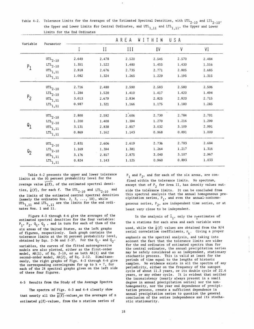
Table 4-2 presents the upper and lower tolerance limits at the 95 percent probability level for the

average value g(f), of the estimated spectral densi­

ties, g (f) , for each f. The UTL2_10 and LTL2_10

and

the limits of the estimated central spectral densities (namely the ordinates Nos. 2, 3, ... , 10), while UTL1, 11 and LTL1, 11 are the limits for the end ordi -

nates Nos. 1 and 11.

Figure 4-3 through 4-6 give the averages of the estimated spectral densities for the four variables: P1

, P2

, Q1

, Q2 , and in turn for each of them of the

six areas of the United States, as the left graphs of figures, respectively. Each graph contains the tolerance limits at the 95 percent probability level, obtained by Eqs . 2-36 and 2-37. For the Q1- and Q2-

variables, the curves of the fitted autoregressive models are also plotted, either as the first-order model, AR(l), of Eq. 2-10, or as both AR(l) and the second-order model, AR(2), of Eq. 2-12. Simultane­ously, the right graphs of Figs. 4-3 through 4- 6 give the corresponding correlograms for up to k = 7, for each of the 24 spectral graphs given on the left side of these four figures.

4-5 Results from the Study of the Average Spectra

The spectra of Figs. 4-3 and 4-4 clearly show

tnat nearly all the g(f)-values,as the averages of n

estimated g(f)-values, from the n station series of

18

P1 and P2, and for each of the six areas, are con­

fined within the tolerance limits. No spectrum, except that of P2 for Area II, has density values out-

side the tolerance limits. It can be concluded from this spectral analysis that the annual homogeneous pre­cipitation series, P1, and even the annual-nonhomo-

geneous series, P2 , are i ndependent time series, or at

least very close to be independent .

In the analysis of z1, only the rlestimates of

the n stations for each area and each variable were

used, while the g(f) values are obtained from the N/ 4 serial correlation coefficients , rk. Giving a proper

emphasis on the spectral analysis, and taking into account the fact that the tolerance limits are wider for the end ordinates of estimated spectra than for the central ordinates, the annual precipitation series may be safely considered as an independent, stationary stochastic process. This is valid at least for the periods of time equal to the lengths of historic samples. No evidence exists in all the spectra of any periodicity, either on the frequency of the sunspot cycle of about 11.3 years, or i ts double cycle of 22.6 years, or any other cycle. It is evident that neither the inconsistency (nearly always present in a small degree in annual precipitation series) nor the non­homogeneity, nor the year end dependence of precipi­tation process, create a sufficient dependence in annual precipitation series to question the general conclusion of the series independence and its stocha­stic stationarity .

Table 4-3. Coefficient of Determination, R2, for the Relationships of the Estimated First Serial Correlation

Coefficient, r 1, and the Estimates of Mean, x, Standard Deviation, sx, Coefficient of Variation,

Cv• as well as Relationships Between these Three Estimates

~ ·-Variable Relationship

VS = versus II

rl vs X 0.0798 0.0020

rl VS x,sx 0.1132 0.0624

pl rl vs i,cv 0.1246 0.0352

X vs s X

0. 7496 0.4693

x VS cv 0.2404 0.1271

rl vs x 0.1618 0.0001

rl vs x,sx 0.1686 0.0086

p2 rl VS x,Cv 0.1699 0.0184

i vs sx 0.8301 0.6458

x vs c v 0 . 3379 0.2071

rl VS x 0 .0068 0.0000

rl vs x,sx 0.0276 0.0184

Ql rl VS i,cv 0.0754 0.0309

X vs s 0.5965 0.6219 X

x vs cv 0.0270 0.0400

rl VS x 0.0051 0.0000

r1 vs x,sx 0.0250 0.0185

Q2 rl vs x,cv 0.1679 0.0838

i vs s 0.6120 0.6212 X

x vs cv 0.0739 0.0406

The spectra of Figs. 4-5 and 4-6 clearly show that they cross the tolerance limits of independent time series for nearly all the areas, with their

average spectral density values, g(f), obtained by

averaging the n estimated g(f)-values for these n stations of the Q1- and Q2-variables. These crossings . exist for most of the six areas. The spectra of g(f) lead to the conclusion that the two series of annual runoff and annual effective precipitation are the 11.e.d. no.U.e. series (with the averages of &stimated densities decreasing with an increase of the frequency). In most cases, the fits of the corresponding first­order autoregressive dependence model , AR(l), or in some cases also of the second-order model, AR(2), show to be the attractive mathematical models for the population processes. The correlograms smoothed by the Parzen function produce also the very smooth spectra of the ll.e.d. no.U. e. type, as opposed to the wfU.te. no.U.e. t ype of spectra for the annual precipitation series.

For all practical purposes, the annual runoff series, as well as the effective annual precipitation (precipitation minus evaporation) series are station­ary but dependent stochastic processes. At least, they can be considered as te.mpo~t.a~t.y 4tationall.y for the sample sizes of available data. These Q

1-

VALUES F 0 R AREA

19

III IV v VI 0.0105 0.0191 0.0839 0.0236

0.0145 0.2356 0.0840 0.0350

0.0168 0.2396 0.0839 0.0352

0 . 7588 0.4012 0. 7100 0.3661

0.0628 0.0187 0.0833 0.0520

0.0007 0.0091 0.0489 0.0002

0.0150 0.0946 0.1676 0.0614

0.0184 0.0897 0.1675 0.0633

0 . 7524 0.3459 0.6697 0.3959

(J-.1660 0.0008 0.0606 0.0470

0.0002 0.0053 0.0003 0.0052

0.0128 0.0215 0.0006 0.0055

0.0694 0.0091 0.3335 0.0155

0. 7284 0.7218 0.6527 0.6986

0. 1622 0.0000 0.0176 0.2233

0.0018 0.0040 0.0000 0.0058

0.0061 0.0131 0.0154 0.0059

0.0240 0.0042 0.3008 0.0322

0.7493 0.7236 0.6475 0.6977

0.1850 0.0000 0.0276 0.0285

and Q2-series do not show any significant periodicity

of the sunspot cycle (11.3 years) , or its double cycle (22.6 years), or any other cycle.

4-6 Relationships Among the Estimates of Parameters of Four Variables for Six Areas

Table 4-3 gi ves the coefficient of determination

(R2), either for the simple correlation (for two esti­

mates of parameters and linear simple correlation), or for the multiple correlation (for three estimates of parameters and linear multiple correlation). First, the estimates of the first serial correlation coef­ficient, r 1, for each series P1, P2, Q1, Q

2, and for

each area, are linearly correlated with x (the mean of the historic series), then with x and s (s • the

X X stand~rd deviation of historic series), and finally with x and Cv (Cv = the coefficient of variation of h . . . ) 2 ~stor~c ser~es . The R -values are given in Table

4-3 in the first three rows for each of the four variables (P1, P2, Q1, Q2). Then, the estimates of

the mean (x) are correlated with the estimates of the

standard deviation s , and then with c , and R2 are X V

given in the forth and fifth rows of each variable in Table 4-3.

I"

P, AREA

g (f) rk 4

0.3

a (f) 0.2 3 _________ _,.,... ---- 0. 1

2 0

-0.1 f k

0 -0.2 0 1.0 2 .0 3 .0 4 .0 5.0 0 2 3 4 5 6 7

4

0.2

------------- 0.1

-0.1

P, AREA 3

0.3 rk

4

0 .2

0 . 1

0

-0.1 f k

-0.2 1.0 2 . 0 3.0 4 .0 5.0 0 2 3 4 5 6 7

Figure 4-3. Average Spectra (The Full Lines of the Left Graphs) with the 95\ Tolerance Limits (The Dashed Lines of the Left Graphs), and the Average Correlograms (The Right Graphs), for the Six Areas {1 , 2, 3, 4, S, 6) of the United States for the n-Series in Each Area of the Annual Homogeneous P 1- Precipitation Series.

First Part of Fig. 4-3. Areas 1, 2, 3.

20

3

AREA 4

0.2

0.1

0 _.--- -------------- ----..

f -0. 1

- 0.2 5.0 0

AREA 5 rk

0.3

0.2

-- -------------~---- ....... 0.1

.... - --------------- ......_, ~ --

- 0 .1 f

0o.____._ __ l ....... o _ _.___2...~...o _ __..__3....~...o_--L.,_4_J.L-o--'--5-.J.o -o. 2 o

g (f) 4

3

1.0

AREA 6 rk

0.3

0.2

- ---------------- 0.1

0 ---0.1

f -0.2

2 .0 3.0 4 .0 5.0 0

Figure 4-3. Conti nued. Second Part of Fig. 4-3 , Areas 4, S, 6.

21

k 2 3 4 5 6 7

k 2 3 4 5 6 7

k 2 3 4 5 6 7

g l f )

g (f) ----------0.2

.------------------ -----......__.~

-0.1 f k

0~--~--~--~--~--~--~L---L---~--~--~ -0.2L-~--~--L-~--~--L-_J

0 1.0 2.0 3.0 4.0

4

3

--------------------

5.0 0

AREA 2 rk

0.3

----

f

2 3 4 5 6 7

k o~--~--~--~--_.--~--~~-~--~--~--~ -0.2~~---L--~--L-~--~--~

0 1.0 2.0 3.0 4 .0 5.0 0 2 3 4 5 6 7

p2 AREA 3

g (f) rk

4 0.3

0.2

0 . 1

--- 0 -----------------------....._,__ - 0 . 1

f k o~--L---L---L-__ L_ __ L_ __ L_ __ L_ __ L_ __ L_~ - 0.2 L----1.--~ __ L___.L __ ....L._~L-_J

0 1.0 2 .0 3.0 4.0 5.0 0 2 3 4 5 6 7

Figure 4-4. Average Spectra {The Full Lines of the Left Graphs), with the 95\ Tolerance Limits (The Light Dashed Lines of the Left Graphs), the Fitted First-Order, AR(l), Autoregressive Model, (The Heavier Dashed Lines of the Left Graphs), and the Average Correlograms (The Right Graphs) for the Six Areas (1, 2, 3, 4, 5, 6) of the United States for the n-Series in Each Area of the Annual Non-Homogeneous P2-Precipitation Series.

First Part of Fig . 4-4, Areas 1, 2, 3.

22

------ ----------- - --- - ------- - --...._ ..__,_

f k o~~--~---L---L--~--L---L-~--~--~ -0.2~~--~~--~--~~~

0 1.0 2.0 3.0 4.0 5.0 0

4

3

g (f)

--- ....... _____ _

AREA 5

rk 0.3

0.2

--- --- ---- 0. 1

---- ----------- --....._"""'

-0.1 f

2 3 4 5 6 7

k -0.2L--L--~~--~--L-~~

0 1.0 2.0 3.0 4.0 5.0 0 2 3 4 5 6 7

p2 AREA 6

g (f) rk

4 0.3

AR( I) g(f) 0.2 3

-- - --- 0. 1

2 0 ------------------------

f -0. 1 k

o~~~~--_.--~--~--~--~--~~--~ -o.2~-L--i-~--~~~~~

0 1.0 2.0 3.0 4.0 5 .0 0 2 3 4 5 6 7

Figure 4- 4. Continued . Second Part of Fig. 4- 4, Areas 4, 5, 6.

23

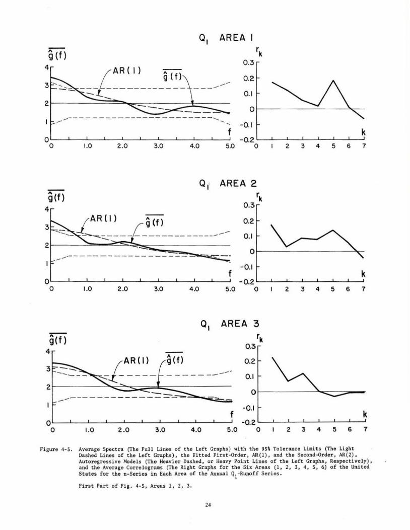
Q1 AREA I

g (f)

0.2

0.1

4

/-

AR(I) g(f)

-==-..- ---- - ----- --0

-0.1 ,.,...-- - - - -- - - - ----- - ------ --...........

~ ' f k

o~--~--~--~--L_ __ L_ __ L_ __ L_ __ L_ __ L_~ -0.2 0 1.0 2.0 3.0 4.0 5.0 0 2 3 4 5 6 7

0 .2

0 .1

0 ,.,,- - - ------ - --- ------

f - 0.1

k o~~~~--~--~--~--~---L--~--~~ -0.2

0 1.0 2.0 3.0 4.0 5.0 0 2 3 4 5 6 7

AREA 3

rk 0.3

g(f) 4

0.2

0.1

0

f -0.1

k OL-~--~---L--~--L-~--~--~--~~ -0.2

0 1.0 2 .0 3 .0 4.0 5 .0 0 2 3 4 5 6 7

Figure 4-5. Average Spectra (The Full Lines of the Left Graphs) with the 95\ Tolerance Limits (The Light Dashed Lines of the Left Graphs), the Eitted First-Order, AR(l), and the Second-Order, AR(2). Autoregressive Models (The Heavier Dashed, or Heavy Point Lines of the Left Gr aphs , Respectively) , and the Average Correlograms (The Right Graphs for the Six Areas (1, 2, 3, 4, 5 , 6) of the United States for the n-Series in Each Area of t he Annual Q1-Runoff Series .

First Part of Fig. 4-5, Areas 1, 2, 3.

24

Ql AREA 4

g(f) rk 0.3

4

0.2

0.1

2 0 . .........:;-. --

f -0.1

k 0 -0.2

0 1.0 2 .0 3 .0 4 .0 5 .0 0 2 3 4 5 6 1

a1 AREA 5

4

0.2

0 .1

0

-....... -0.1 _,....--------------1 _.....

f k 1.0 2.0 3.0 4 .0 5.0 -0.20 2 3 4 5 6 7

a, AREA 6 g(f} rk

4 0.3

g ( f ) 0.2 3 --___________ ___.

0.1

2 0

--- -0. 1 f k

0 -0.2 0 1.0 2.0 3.0 4 .0 5.0 0 2 3 4 5 6 7

Figure 4-5. Continued . Second Part of Fig . 4-5, Areas 4, 5, 6.

25

02 AREA

g(f) rk 0.3

3 ..... ...... .... {:AR (I) g (f) - .__. -- --- -------

2r-------~~ ............ --~~=---------~--------

0 . 2

0.1

,.,,------ ------ - - - - ........ ..... ) -0.1

k 2 .0

-0.2 '--~--'---'----.J----l..._..J__J 3.0 4.0 5.0 0 2 4 5 6 7

a2· AREA 2 g(f)

( AR(f) g (f) 0.2

~ --- -----______ __. 0.1

0

-0.1 f k

0 0 1.0 2.0 3.0 4.0 5.0

-0.2 0 2 3 4 5 6 7

Q2 AREA 3

4 g {f)

rk 0.3

0.2

0.1

0

- 0.1 f k

-0.2 4 .0 5.0 0 2 3 4 5 6 7

Figure 4-6. Average Spectra (The Pull Lines of the Left Graphs) with the 95\ Tolerance Limits (The Light Dashed Lines of the Left Graphs), the Fitted-First Order, AR(l), and the Second-Order, AR(2), Autoregressive Models (The Heavier Dashed, or Heavy Point Lines of the Left Graphs, Respectively) , and the Average Correlograms (The Right Graphs for the Six Areas (1, 2, 3, 4, S, 6) of the United States for the n-Series in Each Area of the Annual Q2-Effective Precipitation Series .

First Part of Pig. 4-6, Areas 1, 2, 3.

26

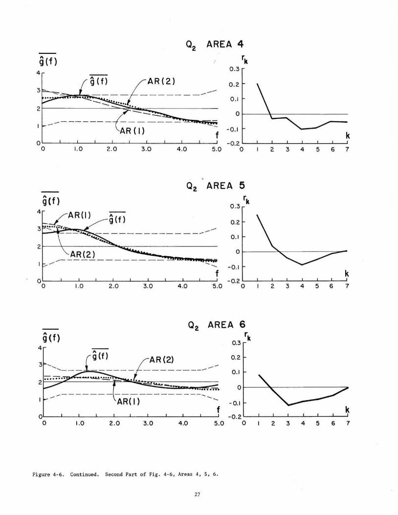
Q2 AREA 4

g (f) 4

0.3

0.2

0.1

AR (I) f -0.1

k o~~--~--~--~--L-~--~--~--~~ -0.2 ~~~~~--~~--L-~

0 1.0 2.0 3 .0 4 .0 5.0 0

1.0

g (f )

0 0 1.0

Q2 AREA 5 r.

0.3 k

0.2 _____________ ,... ..... ..-0. 1

0

...... .........

f -0.1

2.0 3.0 4.0 -0.2

'5.0 0

Q2 AREA 6 ~

0.3 k

0.2

0.1

0

-0.1 f

-0.2 2 .0 3.0 4.0 5.0 0

Figure 4- 6. Continued . Second Part of Fig. 4-6, Areas 4, 5, 6.

27

2 3 4 5 6 7

k 2 3 4 5 6 7

k 2 3 4 5 6 7

The relationships of r 1 versus x , or r 1 versus i

and sx, or r 1 versus x and Cv, show the R2-values (or

the explained variance by the linear correlation) to range between zero and 24% for P1, between zero and

17% for P2, between zero and 8% (except one value of

33%) for Q1, and between zero and 8% (except one value

of 17% and another of 30%) for Q~, in each of four 2 cases (P 1, P 2, Q1, Q2), for a total of 18 values of R .

The only significant correlation found is between

i and sx (the estimates of the mean and standard

deviation are correlated), because whenever xis large, also s is large, or the opposite . However, when x is

X 2 correlated with C = s /x, the R -values are much

V X

smaller then those for sx.

The R2-values can not be considered as signifi­

cant, except for the i versus sx relationships. The

estimates of the first serial correlation coefficient,

r 1, may be considered as independent of the estimates

of the mean, x, the standard deviation, sx' and the

coefficient of variation, Cv . However, the relation­

ships between the estimates x and sx are very signi­

cant. This conclusion is supported by many compu­tations of the past.

4-7 A Retrospective View at the Reliability of Results

The Parzen smoothing funct i on has a bias which depends upon the second derivative of the actual spectrum. This derivative is very smal l in a region where the spectrum is nearly a straight line and very large near a sharp peak. Since the spectral estimates of the series of annual precipitation are serially corr elated only to a very small degree (close to zero),

28

these estimates represent the spectra which are likely to be close to a horizontal line. Thus, the Parzen smoothing function has a small bias most of the t ime . Even for the dependence in the annual runoff series of the order of r 1 = 0.10 - 0.20, th~ bias is small.

The Parzen smoothing function is choosen for the use in this study since it yields no negative values of spectral estima·tes.

It is generally known (particularly for the first-order autoregressive processes [10]) that the increase of the correlogram truncation value m in computing the spectral densities will increase the variance of the estimates and decrease the number of degrees of freedom of their distribution. It results in a wider tolerance interval for the estimates , or a loss of confidence i n the estimates. Furthermore, as it is generally known, an increase in the cor­relogram truncation value m will decrease the bias of the estimate. Most of the time, and for a single spectral estimate, the truncation value m is chosen as an average value for which, hopefully, neither the tolerance interval nor the bias are t oo large. For the purpose of the analysis in this paper, the bias in the spectral estimates was kept to a minimum. How­ever , the variance of the estimates is large, but this is not considered i mportant for the major assumption, namely that each of the n spectral estimates for the n area station series are considered as estimates of the same spectral density of a given frequency. Thus, by combining t he n estimates into the average estimate,

g(f), the variance of this average estimate is greatly reduced (especially for the large number of station series of n = 200-400, with the equivalent ne = 3- 9

for the space independent series). To reduce the bias in the estimates, the truncation value m is taken as high as feasible without jeopardizing the covariance esti mates. The truncation value m is taken as one fourth (1/4) of the sample size, N. To be consistent from sample to sample, this ratio is kept constant for all the series, although the absolute truncation value m changes from sample to sample depending upon the sample size.

Chapter V CONCLUSIONS

The analysis of a large number of station time series of annual precipitation, annual runoff, and annual effective precipitation, leads to these basic conclusions:

(1) For all pract ical purposes, the method of spectral analysis shows that the annual precipitation series in the United States are time independent, stationary stochastic processes; at least, they are tempo~ 6~~ processes for the periods of time of the order of lengths of the available historic series.

(2) The annual runoff series, and from them derived annual effective precipitation series (annual precipitation minus annual evaporation and annual evapotranspiration) in the United States, studied by the spectral analysis , are time dependent, stationary stochastic processes; at least, they are ~empo~ htatiO~ processes for the periods of time of the order of lengths of the available historic series.

(3) The order of the magnitude of the average first serial correlation coefficient for the annual runoff series for many stations of large areas is somewhere between 0.10 and 0. 20-

(4) The major factor responsible for the time dependence of annual series of runoff and effe~tive precipitation is the change from year to year 1n the

water volume stored in river basins.

(5) No significant spectral densities are found for any periodicity, particularly for the sunspot cycle of 11.3 years or its double value of 22.6 years, in annual series either of precipitation or runoff.

(6) It is safe to project the expectations of immediate future , say for the future lengths of times at least equal to the lengths of historic series of precipitation or runoff, that the expected future series of annual precipitation will be very close to independent, stationary stochastic processes, and those of annual runoff very close to dependent, stationary stochastic processes.

(7) For practical purposes, the simple first ­order or second-order autoregressive dependence models seem to be sufficiently accurate mathematical des­cription for the annual runoff series.

(8) By using a very large number of annual time series all over the United States, the time-space study of these processes for data of a relatively short periods of about 30-90 years for various time series, should compensate in some degree for the lack of very long, instrumentally obtained data on precipi­tation and runoff. What is not available in time, it may be somewhat compensated with the information in space, in order to project the near future with a sufficient reliability.

REFERENCES

1. Yevjevich, V., Fluctuations of Wet and Dry Years , Part I, Rest::arch Data Assembly and ~lathe­matical Models, Colorado State University Series of Hydrology Papers, No. l, July 1963.

2. Yevjevich, V., Fluctuations of Wet and Dry Years, Part II , Analysis by Serial Correlation, Colorado State University Series of Hydro­logy Papers, No. 4, June 1964.

3. Milankovitch, M., Canon of Insolation and the Ice­age Problem, translated from German by the Israel Program for Scient ific Translations, Jerusalem 1969: U.S. Department of Commerce, Springfield, Va., 484 pages, 1941 .

4. Vernekar, A. C., Long-period Global Variations of Incoming Solar Radiation, Meteorological Monographs, U.3. Weather Bureau, Vol . 12, No. 34 , 21 pages, 1972.

5. Broecker, W. S., and J. van Dank, Insolation Changes, Ice Volumes, and the 0-18 Record

29

in Deep- sea Cores , Reviews of Geophysics and Space Physics, Vol. 8 , p. 169-198, 1970.

6. Chin, W. Q., and V. Yevjevich, Almost-Periodic, Stochastic Theory of Cl imatic Changes, Colo­rado State University Series of Hydrology Papers , No . 65 , March 1974 .

7. Wiener, Nobert, Extrapolation, Interpolation, and Smoothing of Stationary Time Series (with Engineering Applications), the M.I.T. Press, Cambridge , Mass., 1949.

8. Blackman, R. B., and F. W. Tukey, The Measurement of Power Spectra, Dover Publications, New York 1958.

9. Parzen, Emanuel, Time Series Analysis Papers, Holden -Day, Inc., San Francisco, 1967 .

10. Box, G. E. P. and G. M. Jenkins, Time Series Analysis, Forecasting and Control, Holden­Day, Inc., pp. 553, 1970.

$

Key Words: Wet and Dry Years, Annual Precipitation, Annual Runoff, Time Series Analysis.

Abstract: Spectral analysis is applied to annual series of precipitat ion and runoff. Precipitation series are divided in homogeneous P

1-precipitation

and nonhomogeneous P2-precipitation. Runoff series

are either the observed Q1- series, or they are reduced

to the effective precipitation Q2-series (precipita­

tion minus evaporation). Data of annual preci pitation and annual runoff of a large number of gauging sta­tions in the United States divided in six areas are used in t hi s study.

Key Words: Wet and Dry Years, Annual Precipitation, Annual Runoff, Time Series Analysis.

Abstract: Spectral analysis is applied to annual series of precipitation and runoff. Precipitation series are divided in homogeneous P

1-precipitation

and nonhomogeneous P2-precipitation. Runoff series

are either the observed Q1-series, or t hey are reduced

to the effective precipitation Q2-series (precipita­

tion minus evaporation) . Data of annual precipitation and annual runoff of a large number of gauging sta­tions in the United States divided in six areas are used in this study.

Key Words: Wet and Dry Years, Annual Precipitation, Annua l Runoff, Time Series Analysis .

Abstract: Spectral analysis is applied to annual series of precipitation and runoff. Precipit ation series are divided in homogeneous P

1-precipitation

-· -·- ···----

and nonhomogeneous P2-precipitation. Runoff series

are either the observed Q1

- series, or they are reduced

to the effective precipitation Q2-series (precipit a­

tion minus evaporati on) . Data of annual precipitation and annual runoff of a l ar ge number of gauging sta­tions in the United States divided in six areas are used in thi s study.

Key Words: Wet and Dry Years, Annual Precipitation, Annual Runoff, Time Series Analysis.

Abstract: Spectral analysis is applied to annual series of precipitation and runoff. Precipitation series are divided in homogeneous P

1-precipitation

and nonhomogeneous P2-precipitation. Runoff seri es

are either the observed Q1-series, or they are reduced

to the effecti ve precipitation Q2-series (precipita­

tion minus evaporation). Data of annual precipitation and annual runoff of a large number of gauging sta­t ions in the United States divided in six areas are used in this s tudy.

Techniques of spectral analysis are described. Average spectra are estimated for four variab les (P1,

P2, Q1, Q2) and six areas , with the 95% tolerance

limits.

The annual precipitation series are very close to independent time series, at least temporary stationary for the length of 50-150 years. Annual runoff and annual effective precipitation series are dependent series , at least temporary stationary for the order of l ength of 50-150 years. The first and the second order autoregressive models seem sufficiently accurate for practical use.

Reference: Yevjevich, Vujica; Colorado State University, Hydrology Paper No . 94 (August 1977), Fluctuations of Wet and Dry Years, An Analysis by Variance Spectrum.

Techniques of spectral analysis are described. Average spectra are estimated for four variables (P

1,

P2, Q1, Q2) and six areas, with the 95% tolerance

limits.

The annual precipitation series are very close to independent time series, at least temporary stationary for the length of 50-150 years. Annual runoff and annual effective precipitation series are dependent series, at least temporary stationary for the order of length of 50-150 years. The first and the second order autoregressive models seem sufficiently accurate for practical use.

Reference: Yevjevich, Vujica; Colorado State University, Hydrology Paper No. 94 (August 1977), Fluctuations of Wet and Dry Years, An Analysis by Variance Spectrum.

'

Techniques of spectral analysis are descri bed. Average spectra are estimated for four variables (P

1,

P2, Q1, Q2) and six areas, with the 95% tolerance

l i mits .

The annual precipitation series are very close to independent time series, at least temporary stationary for the length of 50-150 years . Annual runoff and annual effective precipit ation series are dependent series, at least temporary stationary for the order of length of 50-150 years . The first and the second order autoregressive model s seem sufficiently accurate for practical use.

Reference: Yevjevich, Vujica; Colorado State University, Hydrology Paper No. 94 (August 1977), Fluctuations of Wet and Dry Years, An Analysis by Variance Spectrum.

Techniques of spectral analysis are described. Average spectra are estimated for four variables (P

1,

P2, Q1, Q2

) and six areas, with the 95% tolerance

limits .

The annual precipitation series are very close to independent time series, at least temporary stationary for the length of 50-150 years. Annual runoff and annual effective precipitation series are dependent series, at least temporary stationary for the order of length of 50-150 years. The first and the second order autoregressive models seem sufficiently accurate for practical use.

Reference: Yevjevich, Vujica; Colorado State University, Hydrology Paper No . 94 (August 1977), Fluctuations of Wet and Dry Years, An Analys i s by Variance Spectrum.

I I l I I I

t No. 69 ' No. 70

No. 71

No. 72

No. 73

No. 74

No. 75

No. 76

No. 77

No. 78

No. 79

No. 80

No. 81

No. 82

No. 83

No. 84

No. 85

No. 86

No. 87

No . 88

No. 89

No. 90

No. 91

No. 92

No. 93

UST OF PREVIOUS 25 PAPERS

Efficient Sequential Optimization in Water Resources, by Thomas E. Croley II, September 1974.

Regional Water Exchange for Drought Alleviation, by Kuniyoshi Takeuchi, November 1974.

Determination of Urban Watershed Response Time, by E. F. Schulz, December 1974.

generation of Hydrologic Samples, Case Study of the Great Lakes, by V. Yevjevich, May 1975.

Extraction of Information on Inorganic Water Quality, by William L. Lane, August 1975.

Numerical Model of Flow in Stream-Aquifer System, by Catherine E. Kraeger Rovey, August 1975.

Dispersion of Mass in Open-Channel Flow, by William W. Sayre, August 1975.

Analysis and Synthesis of Flood Control Measures, by Kon Chin Tai, September 1975.

Methodology for the Selection and Timing of Water Resources Projects to Promote National Economic Development, by Wendim-Agegnehu Lemma, August 1975.

Two-Dimensional Mass Dispersion in Rivers, by Forrest M. Holly, Jr., September 1975.

Range and Deficit Analysis Using Markov Chains, by Francisco Gomide, October 1975.

Analysis of Drought Characteristics by the Theory of Run, by Pedro Guerrero-Salazar and Vujica Yevjevich, October 1975.

Influence of Simplifications in Watershed Geometry in Simulation of Surface Runoff, by L. J. Lane, D. A. Woolhis·er and V. Yevjevich, January 1976.

Distributions of Hydrologic Independent Stochastic Components, by Pen-chih Tao, V. Yevjevich and N. Kottegoda, january 1976.

Optimal Operation of Physically Coupled Surface and Underground Storage Capacities, by Dragoslav lsailovic, january 1976.

A Salinity Management Strategy for Stream-Aquifer Systems, by Otto J. Helweg, and j. Labadie, February 1976.

Urban Drainage and Flood Control Projects Economic, Legal and Financial Aspects, by NeilS. Grigg, Leslie H. Both am, Leonard Rice, W. ). Shoemaker, and L Scott Tucker, February 1976.

Reservoir Capacity for Periodic-Stochastic Input and Periodic Output, by Kedar Nath Mutreja, September 1976.

Area-Deficit-Intensity Characteristics of Droughts, by Norio Tase, October 1976.

Effect of Misestimating Harmonics in Periodic Hydrologic Parameters, by K. L. Bullard, V. Yevjevich, and N. Kottegoda, November 1976.

Stochastic Modeling of Hydrologic, Intermittent Daily Processes, by Jerson Kelman, February 1977.

Experimental Study of Drainage Basin Evolution and Its Hydrologic Implications, by Randolph S. Parker, June 1977.

A Model of Stochastic Structure of Daily Precipitation Series Over an Area, by C. W. Richardson. July 1977.

Effects of Forest and Agricultural land Use on Flood Unit Hydrographs, by Wiroj Sangvaree and Vujica Yevjevich, July 1977.

A Distributed Kinematic Model of Upland Watersheds, by Edward W. Rovey, David A. Woolhiser and Roger E. Smith, July 1977.