Flight Control Allocation – using Optimization Based ...
155
Flight Control Allocation – using Optimization Based Linear and Quadratic Programming Fall – Project Group DE7-771 7 th Semester AUE 2004
Transcript of Flight Control Allocation – using Optimization Based ...

Flight Control Allocation – using Optimization Based Linear
and Quadratic Programming
Fall – Project Group DE7-771
7th Semester AUE 2004

Flight Control Allocation using Optimization Based Linear and Quadratic programming P7 - project fall 2004 Aalborg Universitet Esbjerg
Title:
Flight Control Allocation using Optimization Based Linear and
Quadratic Programming
Theme: Distributed/Real-time Control Systems
Project period: September 2nd 2004 – December 17th 2004
Project group: DE7-771
Pages: 156
Group members:
Johnny Bakkensen _____________________________
Vasanthan Joseph _____________________________
Uffe Merrild _____________________________
Supervisor: Youmin Zhang
Abstract The performance of constrained optimization algorithms for control allocation with applications to aircraft control was evaluated. Three control allocation algorithms were investigated: A pseudoinverse, a Fixed-point, and a Direct Control Algorithm. The control allocation algorithms include a quadratic programming method and a linear programming method. The algorithms was implemented in the Swedish developed aircraft simulation model, ADMIRE. The aircraft model describes a single-engine delta-wing canard fighter aircraft with 7 control surfaces. The algorithms were both evaluated in a free testing environment to increase analysis clarity, and also in ADMIRE, in order to form a bridge to aircraft applications. The test in the free environment showed quite different results from the algorithm. In general it was stated that all the algorithms performed a solution to the commanded input. However, this was only an issue when none of the output variables was saturated. In the case where some or all of the output variables were saturated the algorithms has trouble achieving the desired moment. Some of them wouldn’t give enough moment and other wouldn’t track the desired moment direction. This was also the issue when the algorithms was tested in ADMIRE.
Page 2 of 154

Flight Control Allocation using Optimization Based Linear and Quadratic programming P7 - project fall 2004 Aalborg Universitet Esbjerg
Table of contents: 1. Introduction................................................................................................................. 5 2. Aerodynamics ............................................................................................................. 5
2.1. Coordinate frames............................................................................................... 5 2.2. Aircraft variables ................................................................................................ 7 2.3. Control variables................................................................................................. 9 2.4. Forces and moments ......................................................................................... 11 2.5. Aerodynamics ................................................................................................... 12 2.6. Gathering the equations .................................................................................... 14 2.7. Control objectives ............................................................................................. 15 2.8. Application of control allocation ...................................................................... 16 2.9. The ADMIRE model......................................................................................... 16
3. Control allocation...................................................................................................... 18 3.1. Control allocation - background ....................................................................... 18 3.2. Control allocation problem formulation ........................................................... 20 3.3. Direct control allocation discussion.................................................................. 22 3.4. Constrained optimization using linear programming ....................................... 22 3.5. Cascaded generalized pseudoinverse method................................................... 23 3.6. Linear programming method ............................................................................ 27 3.7. Fixed-point method........................................................................................... 31
4. Mathematical simulation........................................................................................... 35 4.1. Test of algorithm............................................................................................... 35 4.2. Step input .......................................................................................................... 35 4.3. Ramp input........................................................................................................ 76 4.4. Parabola input ................................................................................................... 84 4.5. Conclusion of mathematical simulation............................................................ 92
5. ADMIRE linear model in simulink........................................................................... 94 5.1. Start the simulation ........................................................................................... 94 5.2. Description of admire_linear_G771_xxx.mdl .................................................. 97
6. Implementation in ADMIRE .................................................................................. 104 6.1. Flight conditions ............................................................................................. 105
7. ADMIRE simulation............................................................................................... 106 7.1. Test 1............................................................................................................... 106 7.2. Test 2............................................................................................................... 110 7.3. Test 3............................................................................................................... 115 7.4. Test 4............................................................................................................... 119
8. Conclusion .............................................................................................................. 125 8.1. Error minimization.......................................................................................... 125 8.2. Control minimization ...................................................................................... 125 8.3. Directionality preservation.............................................................................. 126
9. Control designs for actuator redundancy system.................................................... 127 9.1. Linear Quadratic Regulation with state-feedback........................................... 127 9.2. Summery ......................................................................................................... 149
10. Appendix A......................................................................................................... 150 10.1. Symmetric matrices .................................................................................... 150
11. Aircraft nomenclature ......................................................................................... 153
Page 3 of 154

Flight Control Allocation using Optimization Based Linear and Quadratic programming P7 - project fall 2004 Aalborg Universitet Esbjerg 12. References........................................................................................................... 155 13. Appendix B. .........................................................................................................CD 14. Additional reading ...............................................................................................CD 15. Matlab code..........................................................................................................CD
Page 4 of 154

Flight Control Allocation using Optimization Based Linear and Quadratic programming P7 - project fall 2004 Aalborg Universitet Esbjerg
1. Introduction Control allocation is needed for control of overactuated systems, and deals with distribution of the control effort among the actuators in the system. When using control allocation, the actuator selection task is separated from the regulation task in the control design. In many flight-control systems of the past ganging has been used to associate the three dimensional movements of the aircraft to the control surfaces. For example, to achieve a pitching moment, the left and right elevator deflection should move together while a rolling moment can be produced by the differential movement of the ailerons. As more advanced aircrafts are built, more unconventional control surfaces have been introduced, such as canards, leading-edge flaps and elevons, ganging of these controls is less obvious. This property of the development in aircraft design and also the interest in reconfiguration after failures in flight control has given a solid foundation for the birth of control allocation. The aircraft controller usually outputs the desired moments to be produced in pitch, roll, and yaw. In order to control the aircraft, a mapping from the commanded moments in pitch, roll and yaw onto the control surface deflections needs to be calculated. Since redundant control surfaces are available the solution to determine the deflection of each control surface is not unique. The task of the control allocation algorithm is to provide an optimal mapping based on certain criteria. Three control allocation algorithms have been implemented and tested in the Swedish developed aircraft benchmark “ADMIRE”. These allocation algorithms include a quadratic algorithm as well as a linear, and a fixed-point algorithm. The simulation model, “ADMIRE”, uses a delta-wing canard single engine fighter aircraft model and the aero data is supplied by the Saab AB developed Generic Aerodata Model (GAM). The entire simulation model is implemented in Matlab/Simulink.
2. Aerodynamics In order to understand aircraft control and behavior, a brief introduction to aerodynamics is essential. Any aircraft motion is determined by the moments and aerodynamic forces acting on the aircraft. In the following the moments and forces acting on the particular aircraft we are working on is examined. This section is based on L. Stevens, 2003 and Härkegård 2003.
2.1. Coordinate frames The two frames most frequently used for describing aircraft angles and forces are the earth-fixed frame (i) and the body-fixed frame (b). In the earth-fixed frame the 3 axes are pointing north, east and down. This frame is useful for describing the position and orientation of the aircraft. In the body-fixed frame the 3 axes with origin point at the aircraft centre of gravity are pointing forward, over the right wing and down. In this frame the inertia matrix of the aircraft is fixed thus making the frame suitable for describing angular motions.
Page 5 of 154

Flight Control Allocation using Optimization Based Linear and Quadratic programming P7 - project fall 2004 Aalborg Universitet Esbjerg
Figure 1 Earth-fixed frame (i) and body-fixed frame (b)
Another coordinate frame is the wind-axes frame (w). This frame derives its x-axis from the velocity vector of the aircraft (V). The wind-axis frame is relative to the fixed-body frame by the angle of attack (α) and the angle of sideslip (β) as shown in Figure 1. Given any vector: Eq. 2-1 wwbb vv eev == its component vectors in the first two frames are related by:
Eq. 2-2 w
Twbwbwb
bwbw
vTvTv
vTv
==
=
where:
−−−=
−
−=
ααβαββα
βαββα
αα
βαββββ
cos0sinsinsincossincos
cossinsincoscos
cos0sin010
sin0cos
1000cossin0sincos
wbT
Page 6 of 154

Flight Control Allocation using Optimization Based Linear and Quadratic programming P7 - project fall 2004 Aalborg Universitet Esbjerg Since the body-fixed frame is the most frequently used, the subscript b for component vectors for this frame will not be used further. We will simply write vbev =
Figure 2 Illustration of aircraft orientation angles (φ, θ, ψ) and angular rates (p,q,r)
2.2. Aircraft variables Considering the aircraft as a rigid body its motion can be described by its position, orientation, velocity and angular velocity over time.
2.2.1. Position The position vector is given by: Eq. 2-3 ( )T
ENi hpp −= ep In the earth-fixed frame where pN = position north, pE = position east and h = altitude.
2.2.2. Orientation The orientation of the aircraft can be represented by the Euler angles: Eq. 2-4 ( )Tψθφ=Φ where φ = roll angle, θ = pitch angle and ψ = yaw angle These angles relate the body-fixed frame to the earth-fixed frame.
2.2.3. Velocity The velocity vector (V) is given by: Eq. 2-5 wwb VV eeV ==
Page 7 of 154

Flight Control Allocation using Optimization Based Linear and Quadratic programming P7 - project fall 2004 Aalborg Universitet Esbjerg where:
( )TwvuV = and:
( )TTw VV 00=
in the body-fixed and in the wind-axes coordinate frames respectively. Here u = longitudinal velocity, v = lateral velocity and w = normal velocity and VT = total velocity (airspeed). Eq. 2-6 ( )T
Twbw VVTV βαββα cossinsincoscos==
Conversely, we have that
222 wvuVT ++=
uwarctan=α
TVvarcsin=β
when β = φ = 0 the flight path angle is defined by: Eq. 2-7 αθγ −= as illustrated in Figure 2.
2.2.4. Angular velocity The angular velocity for vector ω is given by: Eq. 2-8 wwb ωω eeω ==
( )Trqp=ω
( )T
wwwwbw rqpT == ωω in the body-fixed and wind-axes coordinates respectively. p = roll rate, q = pitch rate and r = yaw rate. The wind-axes roll rate pw is also known as the velocity vector roll rate since
is parallel to the velocity vector V (see Figure 1). wx
Page 8 of 154

Flight Control Allocation using Optimization Based Linear and Quadratic programming P7 - project fall 2004 Aalborg Universitet Esbjerg
2.3. Control variables The control variables of an aircraft consist of the thrust produced from the engine combined with the control surfaces of the aircraft such as rudder, aileron and elevator. The deflection of the control surfaces produces aerodynamic forces when airflow is forced across them. The engine produces the speed control while the movement in pitch, yaw and roll is determined by the deflections in the control surfaces (δ). In modern aircraft the control surfaces include, but is not limited to, the elevator, aileron and rudder. For both redundancy and performance concerns modern aircraft typically implement more than three control surfaces, see Figure 3. Using this setup, roll control is achieved by deflecting the elevons differentially. Pitch control is achieved by combining symmetric elevon deflection which generate a non-minimum phase response with deflection of the canards which produces a response in the commanded direction immediately.
Figure 3 Modern delta canard fighter aircraft
A growing interest in higher angles of attack has founded the development of thrust vectoring. By mounting deflectable vanes at the engine exhaust it is possible to direct the exhaust to provide additional pitching or yawing moments. Rigid body motion Using the variables in the former section, let us now derive a model of the aircraft dynamics. By considering the aircraft as a rigid body allows us to use Newton’s laws of motion to investigate the effects of the external forces and moments acting on the aircraft. In the earth-fixed frame (i), Newton’s second law states that:
Eq. 2-9 ( )VF mdtd
i
=
Page 9 of 154
Flight Control Allocation using Optimization Based Linear and Quadratic programming P7 - project fall 2004 Aalborg Universitet Esbjerg
HTidt
d=
Where F = total force, T = total torque, m = aircraft mass and H = angular momentum of the aircraft. Using Figure 1 allows us to perform the differentiation in the body-fixed frame instead.
Eq. 2-10 ( ) VωVF mmdtd
b
×+=
HωHT ×+=bdt
d
As this frame is relative to the aircraft, the inertia matrix I is constant. The angular momentum can be expressed as: Eq. 2-11 IwbeH = where:
−
−=
zxz
y
xzx
III
III
000
0
The zero-entries are a property of the aircraft symmetry around the xz-axis. Expressing all vectors in the body-fixed frame gives the following standard equations for rigid body motion in terms of velocity and angular velocity: Eq. 2-12 ( )VVmF ×+= ω
ωωω IIT ×+= Pitch, yaw and roll angle dynamics during level flight are given by: Eq. 2-13 p=φ
rq
==
ψθ
Page 10 of 154

Flight Control Allocation using Optimization Based Linear and Quadratic programming P7 - project fall 2004 Aalborg Universitet Esbjerg
2.4. Forces and moments In Eq. 2-9 F and T represent the sum of forces and moments acting on the aircraft at the centre of gravity. These forces are a combination of three major forces; gravity, engine thrust and aerodynamic effects. F and T can therefore be expressed as: Eq. 2-14 AEG FFFF ++=
AE TΤT += We will now briefly investigate these components.
2.4.1. Gravity Gravity only gives a force contribution since it acts at the aircraft center of gravity. The gravitational force mg is directed along the normal of the earth plane and is considered to be independent of the altitude. This gives:
=
−=
=
3
2
1
sincoscossin
sin00
ggg
mmgmg
wbiG eeeFθφθφ
θ
where:
Eq. 2-15
( )( )( )θφαθα
θφβαθφβθβαθφβαθφβθβα
coscoscossinsincoscossinsincossincossinsincos
coscoscossincossinsinsincoscos
3
2
1
+=−+=
++−=
gggggg
using rotation around the 3 axes in Figure 2.
2.4.2. Engine The thrust force produced by the engine is denoted by Ft. Assuming the engine is positioned to produce a force parallel to the aircraft body axis gives:
Eq. 2-16
=
00
T
bE
FeF
Also assuming the engine is positioned so the thrust point lies in the xz-plane of the body-fixed frame offset from the center of gravity by zTP along the z-axis gives a pitching moment:
Page 11 of 154

Flight Control Allocation using Optimization Based Linear and Quadratic programming P7 - project fall 2004 Aalborg Universitet Esbjerg
Eq. 2-17
=
0
0
TPTbE zFeT
If thrust vectoring is used these expressions become different and depend also on the engine nozzle deflections.
2.5. Aerodynamics The aerodynamic forces and moments are generated by the interaction between the aircraft body and the surrounding air. The size and direction of the moments are determined by the amount of air diverted by the aircraft in different directions. The amount of air directed by the aircraft is determined by:
• The speed and density of the airflow (VT, ρ) • The geometry of the aircraft: S (wing area), b (wing span), c (mean aerodynamic
chord) • The orientation of the aircraft relative to the airflow: α, β • The control surface deflections: δ
Figure 4 Aerodynamic forces and moments in the body-fixed frame
The aerodynamic forces and moments also depend on other variables, such as angular rates (p,q,r) and the time derivatives of the aerodynamic angles ( ) but these effects are not as prominent. This motivates a standard way of modeling scalar aerodynamic forces and moments:
βα ,
Page 12 of 154

Flight Control Allocation using Optimization Based Linear and Quadratic programming P7 - project fall 2004 Aalborg Universitet Esbjerg
Eq. 2-18 ( )
( )...,,,,,,,
...,,,,,,,
βαβαδ
βαβαδ
rqpSlCqMoment
rqpSCqForce
M
F
=
=
where the aerodynamic pressure is given by:
Eq. 2-19 ( ) 2
21
TVhq ρ=
The aerodynamic pressure captures the density dependence and most of the speed dependence. The remaining aerodynamic effects are determined by the dimensionless aerodynamic coefficients Cf and Cm. These coefficients are difficult to determine analytically but can be estimated empirically through wind tunnel experiments and actual flight tests. Typically each coefficient is written as the sum of several components each capturing the dependence of one or more of the variables involved. These components can be represented in several ways. A common approach is to store them in look-up tables and use interpolation to compute intermediate values. In other approaches one tries to fit the data to some parameterized function. In the body-fixed frame we introduce the components:
Eq. 2-20 where
=
ZYX
bA eF
z
y
x
SCqZ
SCqYSCqX
=
=
=
Eq. 2-21 where
=
NML
bA eT)momentyawing(
)momentpitching()momentrolling(
n
m
l
SbCqNCcSqM
SbCqL
==
=
These are illustrated in Figure 4. The aerodynamic forces are often expressed in the wind-axes coordinate frame:
Eq. 2-22 where
−
−=
LY
D
wA eF)forcelift()forceside()forcedrag(
L
Y
D
SCqLSCqYSCqD
===
The sign convention is such that the drag force acts along the negative xw-axis in Figure 1 while the lift force is directed upwards perpendicular to the velocity vector. Using Eq. 2-2 the force components in the two frames are related by:
Page 13 of 154

Flight Control Allocation using Optimization Based Linear and Quadratic programming P7 - project fall 2004 Aalborg Universitet Esbjerg
Eq. 2-23
ααβαββαβαββα
cossinsinsincossincoscossinsincoscos
ZXLZYXYZYXD
−=−+−=
−−−=
The lift force (L) opposes gravity and prevents the aircraft from falling down. The lift generated is mainly produced from the angle of attack (α).
Figure 5 Lift coefficient as function of angle of attack in ADMIRE
Figure 5 shows the lift coefficient CL as a function of the angle of attack for the ADMIRE model. An increase in angle of attack leads to an increase in lift coefficient up to an angle of 32° where CL reaches its maximum. Beyond this angle of attack, the lift decreases. This point is called the stall angle, which civil aircraft wants to avoid during flight – while military aircraft can draw advantage of higher angles of attack for tactical purposes.
2.6. Gathering the equations The equations which describe the rigid body dynamics (section 0) and forces and moments (section 2.4) can be gathered to describe the full motion of the aircraft. Combining Eq. 2-12 with Eq. 2-14 yields : Body-axes force equations:
Eq. 2-24
( )( )
)(coscoscossinsin
qupvwmmgZpwruvmmgYrvqwummgFX T
−+=+−+=+
−+=−+
θφθφθ
Body-axes moment equations:
Page 14 of 154

Flight Control Allocation using Optimization Based Linear and Quadratic programming P7 - project fall 2004 Aalborg Universitet Esbjerg
Eq. 2-25
( )( ) ( )
( ) qrIpqIIpIrIN
rpIprIIqIzFM
pqIqrIIrIpIL
xzxyxzz
xzzxyTPT
xzyzxzx
+−+−=
−+−+=+
−−+−=22
The force equations can also be expressed in the wind-axes coordinate frame in terms of VT, α, β, ωw which gives the following equations:
Eq. 2-26
( )
( )
( )2
3
1
sincos1
sin1cos
1
coscos1
mgFYmV
r
mgFLmV
q
mgFDm
V
TT
w
TT
w
TT
+−+−=
+−−+=
++−=
βαβ
αβ
α
βα
In the absence of lateral motion, i.e when p = r = φ = β = 0, the equations of motion in the longitudinal direction are given by:
Eq. 2-27
( )
( )
( )
( )TPTy
TT
TT
TT
zFMI
q
q
mgFLmV
mgFLmV
q
mgFDm
V
+=
=
−+=
+−−+=
−+−=
1
cossin1
cossin1
sincos1
θ
γαγ
γαα
γα
2.7. Control objectives Flight control systems can be designed for several types of control objectives. Let us first consider general maneuvering. In the longitudinal direction the normal acceleration is defined as:
Eq. 2-28 mgZnz −=
The pitch rate (q) can be selected as the controlled variable. The pitch rate is sometimes referred to as the normal acceleration. The normal acceleration or load factor (this factor
is often used for the lift-to-weight ratio mgLn = ) is the normalized aerodynamic force
Page 15 of 154

Flight Control Allocation using Optimization Based Linear and Quadratic programming P7 - project fall 2004 Aalborg Universitet Esbjerg along the negative body-fixed z-axis, expressed as a multiple of the gravitational acceleration (g). The normal acceleration is closely coupled with the angle of attack (α). Since α appears naturally in the equations of motion (Eq. 2-27) angle of attack command control is also common in particular for nonlinear approaches. For lateral control, roll rate and sideslip command control is most often chosen. For roll-control the body-fixed x-axis may be selected as the rotation axis and p as the controlled variable. At high angles of attack however, this choice leads to a disadvantage from the property of a rolling motion, which produces sideslip from the angle of attack. This property quickly leads to problems since the largest sideslip during a rolling motion is in the order of 3-5 degrees. To remove this effect the rotation axis can instead be selected as the x-axis of the wind-axes frame which means pw is the controlled variable. The resulting maneuver is known as velocity vector roll.
2.8. Application of control allocation In flight control applications control allocation means computing control surface deflections such that the demanded aerodynamic moments are produced. This requires a static relationship between the commanded control deflections and the resulting moments, i.e. servo dynamics need to be neglected. For linear control allocation methods to be applicable the aerodynamic forces and moments must be affine in the control deflections. In terms of the aerodynamic coefficients in Eq. 2-18 this means:
Eq. 2-29 ( ) ( ) ( )( ) ( ) ( )δδ
δδxbxaxC
xbxaxC
MMM
FFF
+=+=
,,
must hold, where ( )...,,,, rqpx βα=
2.9. The ADMIRE model To evaluate the designed control allocation algorithms produced in this project, the ADMIRE model is used for simulation. The ADMIRE model consist of a single engine delta-canard wing fighter aircraft model implemented in Matlab/Simulink and is maintained by the Department of Autonomous Systems of the Swedish Research Agency (FOI).
Page 16 of 154

Flight Control Allocation using Optimization Based Linear and Quadratic programming P7 - project fall 2004 Aalborg Universitet Esbjerg
Figure 6 ADMIRE control surface configuration
Further details about ADMIRE:
• Dynamics: The dynamic model consists of the nonlinear rigid body equations along with the corresponding equations for the position and orientation. Actuator and sensor dynamics are included.
• Aerodynamics: The aerodata model is based on the Generic Aerodata Model (GAM) developed by Saab AB and was recently extended for high angles of attack.
• Control surfaces: The actuator suite consist of canards (left and right) leading-edge flaps (left and right), elevons (inner, outer, right and left), a rudder and thrust vectoring capabilities. In this project the leading edge flaps will not be used for control allocation since these do not produce large aerodynamic moments. Thrust vectoring will also not be used in this project as a cause of lacking documentation. The remaining seven control surfaces are denoted in Figure 6. u denotes the commanded deflection while δ represent the actual deflection.
• Actuator models: The servo dynamics of the utilized control surfaces are given by first order systems with a time constant of 0.05s, corresponding a bandwidth of 20 rad/sec. Actuator position and rate constraints are also included.Table 1 shows the actual rate and position constraints for flight below Mach 0.5.
• Flight envelope: The flight envelope covers Mach numbers up to 1.2 and altitudes up to 6000m. Longitudinal aerodata exist up to an angle of attack of 90 degrees, while lateral aerodata only exist for angles of attack up to 30 degrees.
Table 1 ADMIRE control surface limits below Mach 0.5 Control surface Min. deflection(deg) Max deflection(deg) Max. rate (deg/sec) Canards -55 25 50 Elevons -30 30 150 Rudder -30 30 100
Page 17 of 154

Flight Control Allocation using Optimization Based Linear and Quadratic programming P7 - project fall 2004 Aalborg Universitet Esbjerg
3. Control allocation As described earlier, control allocation is a mapping from the desired moments and forces into deflections of the control surfaces. In a modern control system the control allocator block is placed between the actuators and the designed controller. See Figure 7. The algorithms implemented into this block must be chosen amongst many different constrained optimization based algorithms. These include but are not limited to: least-squares, linear programming and quadratic programming.
Control law
Controlallocator Actuators System
dynamicsv u
r y
x
δ
Figure 7 Control allocation block diagram
The simplest control allocation method is based on the unconstrained least squares algorithm with small modifications to consider position limits of the actuators. More complex methods are derived from the constrained least squares optimization to solve the control allocation problem. Until recently it was believed that control allocation was too complex and computational intensive for real world use in flight control cases. However, the recent dramatic change in computer speed and the development of more efficient algorithms have changed the situation considerably. In this project a few of the algorithms for control allocation are tested in the ADMIRE Matlab/Simulink model. The ADMIRE model used is the linear model, to provide for a brief overview of the aspect of control allocation with respect to applications of flight control.
3.1. Control allocation - background To introduce the ideas behind control allocation, consider the system: Eq. 3-1 21 uux += Where x is a scalar state variable, and u1 and u2 are control inputs. x can be affected by two actuators. Assume that to accelerate the object, the net force v = 1 is to be produced. There are several ways to achieve this. We can choose to utilize only the first actuator and select u1 = 1, u2 = 0, or to gang the actuators and use u1 = u2 = 0.5. In linear control theory, there is a wide range of control design methods, like LQ design, which perform control allocation and regulation in one step (Härkegård 2003). Thus, the usefulness of control allocation for linear systems is not so obvious. There are however other, more practical reason to use a separate control allocation module, even for linear system. One benefit is that actuator constraints can be taken into account. If one or more actuator saturates, and fail to produce its nominal control effect, another actuator may be used to make up the difference.
Page 18 of 154

Flight Control Allocation using Optimization Based Linear and Quadratic programming P7 - project fall 2004 Aalborg Universitet Esbjerg
3.1.1. Linear equations The linear equations can be divided in to three groups:
( ) 0=ji xf Where
11 , nxj
mxi RxRf ∈∈
• Under-determined system m < n (fewer equations than unknowns) • Over-determined system m > n (more equations than unknowns) • Exact-determined system m = n (same number of equations and unknowns)
Under-determined system m < n An underdetermined system (m < n) does not have a unique solution, it can be consistent with infinitely many solutions or inconsistent, with no solution. If underdetermined system has infinite number of solutions, then we can not find the solution by x = A+b = AT(AAT)-1b. Then it gives minimum - norm solution with smallest ||x||. Over-determined system m > n In this case there is more equations than unknowns (m > n) in the system and it is usually inconsistent and does not have any solutions. Exact-determined system m = n In this case is the system consistent and there is only one solution.
3.1.2. Optimization – mathematical Background An optimization problem can generally be described as determining values of independent variables that correspond to a “best” or optimal solution of a function. Chapra (2002, p. 336) defines optimization as; find x1 which minimizes or maximizes f(x) subject to:
Eq. 3-2 ( )( ) nibe
miad
ii
ii
,,2,1,,2,1
===≤
xx
where x is an n – dimensional design vector, f(x) is the objective function, di(x) are inequality constraints, ei(x) are equality constraints, and ai and bi are constraints. Optimization problems can be classified on basis of the form of f(x):
• If f(x) and the constraints are linear we have linear programming. • If f(x) is quadratic and the constraints are linear, we have quadratic programming.
Page 19 of 154

Flight Control Allocation using Optimization Based Linear and Quadratic programming P7 - project fall 2004 Aalborg Universitet Esbjerg
• If f(x) is not linear or quadratic and the constraints are nonlinear, we have nonlinear programming.
The constraints considered in the control allocation problems, relate only to position constraints in the actuator suite of the aircraft. These constraints are regarded as equality constraints in the implemented methods. Given a virtual control command v, determine a feasible control input u such that Bu=v. this can be considered in the following way:
• If there are several solutions, pick the best. • If there is no solution, determine u such that Bu approximates v as possible.
lp – norm can be used when we want to analyze how good the measured solution or approximation is. The lp – norm of a vector u ∈ Rm is defined as,
Eq. 3-3 ∞≤≤
= ∑
=
pforupm
i
pip
1
1
1u
and the optimal control input is given by the solution to a two – step optimization problem given as,
( )( )
pvuuu
pduu
vuBw
uuwu
−⋅=Ω
−=
≤≤
Ω=
maxmin
minarg
minarg
Interpretation: Given Ω, the set of feasible control inputs that minimize Bu-v (weighted by wv), pick the control input that minimizes u-ud (weighted by wu) ud – desired control input wu, wv – weighting matrix
3.2. Control allocation problem formulation Before beginning to examine control allocation in more detail, the initial problem must first be defined. Consider the state-space model:
Eq. 3-4 Cxy
BuAxx=
+=
where are all vectors. For control of the aircraft the state vector x can include the angle of attack, the angle of sideslip and the pitch rate. The output vector y might contain the pitch rate, roll rate and yaw rate. The control input vector u contains the actuator position deflections if the actuator dynamics are neglected. If the control surfaces are ganged the number of control variables can be as small as 3, otherwise the number of control variables (p) are usually in the range from 5 to 20.
111 ,, mxpxnx RRR ∈∈∈ uyx
Page 20 of 154

Flight Control Allocation using Optimization Based Linear and Quadratic programming P7 - project fall 2004 Aalborg Universitet Esbjerg Model reference control laws rely on a reference model which represents the desired dynamics of the closed-loop system. Consider the following reference model: Eq. 3-5 MMMMM rByAy += where rM is a reference input vector, in this case the commands from the pilot and yM represents the desired output of the system. Because the derivative of y is given by: Eq. 3-6 BuCAxy += the objective can be achieved by setting: Eq. 3-7 ( )MMM rByACAxBu ++−= −1
Model matching follows if the matrix B is square and invertible and if the original system is minimum phase (Bodson 2002, p. 704). If the matrix B is not square but full row rank (has more columns than rows, as in the case with redundant actuators), the same model reference control law can be used if one defines the desired control effect vector (v) as: Eq. 3-8 MMM rByACAxv ++−= and a control input u such that: Eq. 3-9 ( ) vuB = To obtain u from Eq. 3-9 one must solve a system of linear equations with more unknowns than equations. Although this might seem like an easy task, the vector u is constrained. The limits generally have the form: Eq. 3-10 ,ii,i uuu maxmin ≤≤ for i = 1,…,p
These constrains originate from the actuator position or rate limitations of the physical system. Given the limits, an exact solution might not exist, despite of the redundancy. Further, even if an exact solution exists, it cannot be assumed to be unique. Finding a solution to Eq. 3-9 within the constraints from Eq. 3-10 is defined as the control allocation problem. In the light of this problem formulation, the control allocation can be further formulated into 4 categories using mathematical formulations. These formulations all take into consideration that a solution is not unique and might not exist.
Page 21 of 154

Flight Control Allocation using Optimization Based Linear and Quadratic programming P7 - project fall 2004 Aalborg Universitet Esbjerg
3.2.1. Direct allocation problem Given a matrix B, find a real number a and a vector u1 such that J = a is maximized, subject to: Eq. 3-11 ( ) vuB a=1
and u . maxmin uu ≤≤If a > 1, let:
a1uu = . Otherwise let 1uu =
An advantage of direct allocation includes the straightforwardness of the allocation problem. No design variables must be selected, since the solution to the problem is determined by the control effectiveness matrix (B) and the constraints. When a>1 no element in u will be saturated. A method of implementing direct allocation is by using linear programming.
3.3. Direct control allocation discussion The objective of direct control allocation is to find a control vector u which gives the best approximation of v in the given direction. Thus direct control allocation weighs directionality over moment generation, which is an important characteristic especially for applications such as flight control. In a special case of the matrix B direct allocation provides a unique solution to the problem. The condition for this property is that any q rows of B must be linearly independent, where q is the number of rows in B (Bodson, 2002). In flight control the case is most often that the rows in B are 3. In this case the three components of v in the model reference control law is the accelerations in p, q and r as outputs are three rotational accelerations. The columns of B represent the contributions of the various control surfaces to each of the three rotational accelerations.
3.4. Constrained optimization using linear programming Linear programming (LP) is an optimization approach that deals with meeting a desired objective such as minimizing cost in the presence of linear constraints such as limited resources. Standard form: The basic linear programming problem, consist of two major parts:
• The objective function, and • A set of constraints
The maximization problem, the objective function expressed as:
Page 22 of 154

Flight Control Allocation using Optimization Based Linear and Quadratic programming P7 - project fall 2004 Aalborg Universitet Esbjerg
nn xcxcxcxc ++++= 332211max Z Where cj = payoff of each unit of the jth activity that is undertaken and xj = magnitude of the jth activity. The constraints can be considered as:
iininiiiiii bxaxaxaxa ≤++ 332211 where aij = amount of the ith resource that is consumed for each unit of the jth activity and bi = amount of the ith resource that is available. That is, the resource is limited. The second general type of constraint specifies that all activities must have a positive value.
0≥ix Together, the objective function and the constraints specify the linear programming problem.
3.5. Cascaded generalized pseudoinverse method Most existing methods for control allocation can be classified as pseudoinverse methods. If we disregard the actuator constraints, these methods can be reduced from the algorithm (Härkegård 2003, p. 123):
( )( )
pvuuu
pduu
vBuw
uuwu
−=Ω
−=
≤≤
Ω=
maxmin
minarg
minarg
to
( )2
min duuu −
Subject to Bu=v Which has an explicit solution given by Eq. 3-12 v+= Bu Where B+=BT(BBT)-1 is the pseudo inverse of B. The l2 – norm is the most frequently used method because it can be beneficial to use on the behave of it is a linear program which is much faster than a quadratic program.
Page 23 of 154

Flight Control Allocation using Optimization Based Linear and Quadratic programming P7 - project fall 2004 Aalborg Universitet Esbjerg As stated above, the psoudoinverse solution Eq. 3-12 will not be feasible for all attainable virtual control inputs v. various ways to accommodate to the constraints have been proposed. The simplest alternative is to truncate Eq. 3-12 by clipping those components that violate some constraint. However, since this typically causes only a few control inputs to saturate, is seems natural to use the remaining control inputs to make up the difference. Virnig and Bodden (Härkegård 2003, p. 124) propose a Redistributed PseudoInverse (RPI) scheme, in which all control inputs that violate their bounds in the pseudoinverse solution are saturated and removed from the optimization. Then, the control allocation problem is resolved with only the remaining control inputs as free variables. Bordignon (Härkegård 2003, p. 124) proposes an iterative variant of RPI. Instead of only redistributing the control effect once, the author proposes to keep redistributing the inputs as they become saturated. This is known as the Cascaded Generalized Inverse (CGI) approach. The method of CGI arises from the idea that if a generalized inverse commands a control to exceed a position limit, then that control should be set at the exceeded limit, and the rest of the controls redistributed to achieve the desired moment. This procedure can be used with either pseudoinverse, or generalized inverse weighted with a diagonal matrix. Initially, a generalized inverse is computed using either: Eq. 3-13 ( ) 1−+ = TT BBBB or Eq. 3-14 ( ) ( )( ) 1−+ = TT BNBNBNNB This matrix is used to allocate the controls given in response to some desired moment. Eq. 3-15 v+= Bu If none of the elements in the solution is saturated, then the desired moment lies within the limits of the constraints. If any of the elements in the solutions exceeds their constraints, the element is set equal to its constraint, and their effects at saturation are subtracted from the desired moment. The effect of a saturated control is equivalent to the control position multiplied by the column of the B matrix which corresponds to that control. The resulting moment is the part of the moment demand that must be satisfied by the remaining controls which is denoted ur. For example, if the ith control saturates: Eq. 3-16 ( ) (satiirsatii uuu Bu )−= ,
Next, the saturated controls are removed from the problem. When a pseudoinverse is used, this is done by removing the corresponding column, Bi, from B. The reduced B matrix is denoted B*. The new pseudoinverse is then computed by plugging B* into Eq.
Page 24 of 154

Flight Control Allocation using Optimization Based Linear and Quadratic programming P7 - project fall 2004 Aalborg Universitet Esbjerg 3-13 or Eq. 3-14 to get B*+. Now the new solution is once again checked for saturation. If there is saturated elements, the algorithm runs one more time according to the above method. Ultimately, either no new control will be saturated, or all the remaining controls are saturated, or the reduced B will have n or fewer columns. When no new controls are saturated, an admissible solution is found. If all the controls are saturated, the controls are set to their limits and the moment is unattainable using this method. In the following we will try to demonstrate the concept of the CGI through an example.
3.5.1. An example Take the case where:
[ ]12=B v = 3.5 The constraints are as follows:
2010
2
1
≤≤≤≤
uu
The initial values for ud is given by:
[ ]Td 00=u The pseudoinverse solution is given by:
=⋅
=⋅=
+
7.04.1
5.32.04.0
2
1 vuu
B
u1 is infeasible since this control saturates at u1 = 1. The control allocation problem is resolved with only u2 as free variable. Replacing the original B matrix by [ 10 ]~ =B the virtual control input that should be produced by u2 is given by
[ ]5.125.3
012~1
=−=⋅+⋅−= uvv
And the solution is then given by:
5.15.11~~2 =⋅=⋅= + vBu
which is feasible since v= 2·1+1.5=3.5 and the algorithm stops. In this case, Cascade Generalized Inverse (CGI) was successful since the output:
Page 25 of 155

Flight Control Allocation using Optimization Based Linear and Quadratic programming P7 - project fall 2004 Aalborg Universitet Esbjerg
=
=
5.11
2
1
uu
u
is the true solution, though this is not always true.
0 21
1
0
2
ud
u1
u
u2
u1 Figure 8 Successful case
An example where the algorithm fails to find the optimal solution could be if the constrains in the above example was set to
2110
2
1
≤≤≤≤
uu
Running the algorithm with this constrains will after the first iteration set u1 = 1.4 and u2 = 0.7 And after the constraints are inserted u1= u2 = 1 this will give the result
=
=
11
2
1
uu
u
which is an incorrect result.
0 21
1
0
2
ud
u1uu2
u1 Figure 9 Failing case
Using CGI it is not guaranteed that the optimal solution is found.
Page 26 of 155

Flight Control Allocation using Optimization Based Linear and Quadratic programming P7 - project fall 2004 Aalborg Universitet Esbjerg
3.6. Linear programming method Bodson re-formulated direct control allocation as a linear programming problem by e-mail the 27th November 2004, and based on this definition, we can derive the following linear programming problem. When re-defining the control allocation problem to fit into linear programming formulation, a standard form must be followed. Linear programming implies this standard form: Eq. 3-17 bAx ≤ subject to: Eq. 3-18 maxmin xxx ≤≤ In our optimization problem, we must find a vector x which minimizes: Eq. 3-19 xcTJ = subject to: Eq. 3-20 , h≤≤ x0 bAx = To obtain a linear programming problem in its standard form from the control allocation problem, a matrix M must be defined. The largest element of v must be identified beforehand. The largest element in v is denoted vmax, while the two remaining elements of v are defined as v1 and v2. According to the position of the largest element in v, M is defined. The index of M corresponds to the position of the largest element in v. The matrix M is then defined as one of three cases:
Eq. 3-21 M , ,
−
−=
2max
1max3 0
0vvvv
−
−=
max3
1max2 0
0vv
vvM
−
−=
max3
max21 0
0vv
vvM
Using this M matrix, we can define the linear programming problem in standard form, by defining the matrix A, the vectors b, h and cT. We proceed by defining A: Eq. 3-22 BMA *= We need A to define b, which is then defined as: Eq. 3-23 minxAb ⋅−= Proceeding to define h, we have:
Page 27 of 155

Flight Control Allocation using Optimization Based Linear and Quadratic programming P7 - project fall 2004 Aalborg Universitet Esbjerg Eq. 3-24 minmax xxh −= The objective function (cT) must also be defined according to the problem. We define cT as: Eq. 3-25 vBc TT −= The equations are then set up in a standard linear programming tableau, and the linear programming problem is then solved. In our implementation the MATLAB function “linprog” is used. The solution vector (x) must then be scaled according to the scaling factor (a). According to the value of the scaling factor, a logical choice is made to determine whether or not the solution vector should be scaled. If the scaling factor is larger than one, the solution vector should be. The scaling factor is calculated as:
Eq. 3-26 ( )( )T
T
avv
vBu⋅
=
3.6.1. An example Using the data from the example from the pseudoinverse method, we have:
Eq. 3-27 ,
=
=
090
3
2
1
vvv
v
=
110010100001
B
Where ≤ .
≤
12
105
1-2-
10-5-
u
We proceed by defining M. Since the largest element of v is v2, M is defined as:
Eq. 3-28
−
−=
900009
M
Following the procedure described above and using Eq. 3-22, we define A:
Page 28 of 155

Flight Control Allocation using Optimization Based Linear and Quadratic programming P7 - project fall 2004 Aalborg Universitet Esbjerg
Eq. 3-29
−=
−
−=
00000009
110000100001
900009
A
Using Eq. 3-23 we define b:
Eq. 3-30
−−
=
−−−−
⋅
=
2745
12105
99000009
b
Using Eq. 3-24 we define h:
Eq. 3-31
=
−−−−
−
=
242010
12105
12105
h
Using Eq. 3-25 we define the objective function (cT).
Eq. 3-32
−
−=
⋅
−−−
−−
=
9090
090
110100010001
Tc
Writing the linear programming tableau, we define the following:
X1 X2 X3 X4 b c 0 -9 0 -9 0
R1 -9 0 0 0 -45 R2 0 0 -9 -9 -27
Where row c is the objective function and R1 and R2 are the rows of A. Looking at the objective function, it can be seen that we must increase X2 and X4 to obtain a better value of the objective function. To do this, both X2 and X4 is driven to their saturated values. X2 = 20, X4 = 2. We obtain the following tableau:
Page 29 of 155

Flight Control Allocation using Optimization Based Linear and Quadratic programming P7 - project fall 2004 Aalborg Universitet Esbjerg
X1 X3 b c 0 0 0
R1 -9 0 -45 R2 0 -9 -9
This gives an easy solution for both X1 and X3. X1 = 5 and X3 = 1 The x vector then becomes:
Eq. 3-33
=
21205
x
Before we arrive at the final solution, we must first return from the linear programming problem definition, and obtain a formulation for use with the control allocation problem. Continuing to use Bodson’s formulation, we calculate:
Eq. 3-34
−=+=
11
100
minxxu
At last, the scaling factor must be calculated and applied to the solution if appropriate. Using the following formula, the scaling factor is calculated:
Eq. 3-35 ( )( ) 81
99=
⋅= T
T
avv
vBu
Since a>1, all elements of u must be divided by a to complete the calculations. This gives a final solution of:
Eq. 3-36
−=
8181.08181.01818.8
0
u
In order to find out whether this solution produces the right moment in the right direction, we can calculate:
Page 30 of 155

Flight Control Allocation using Optimization Based Linear and Quadratic programming P7 - project fall 2004 Aalborg Universitet Esbjerg
Eq. 3-37
=
−⋅
==
090
8181.08181.01818.8
0
110010100001
Buv
This calculation concludes that the solution found using linear programming is correct.
3.7. Fixed-point method The fixed-point algorithm is simple. Many of the computations need to be performed only once before iterations starts. Remarkably, the algorithm also provides an exact solution to the optimization problem, and it is guaranteed to converge. Its drawback is that convergence of the algorithm can be very slow and strongly dependant on the problem. (The number of iterations required can vary by orders of magnitude depending on the desired vector.) In addition, the choice of the parameter ε is delicate, as affects the objectives, as well as the convergence of the algorithm. Bodson (2002). The fixed-point method is based upon the mixed allocation problem. This section is based on Härkegård (2003). The fixed-point method finds the control input vector u that minimizes:
Eq. 3-38 ( ) 2
2
2
21 uvBu εε +−−=J
subject to umin ≤ u ≤ umax In this case we use l2 – norm and consider the initial value ud = 0. The algorithm becomes:
Eq. 3-39 ( ) ( )[ ]
( )k
kT
k nnsatGuFv
uIMvBu−=
−−−=+ ε11
where: Eq. 3-40 ( ) IBM εε +−= T1 and:
Eq. 3-41 2
1M
=n
Sat (·) is the saturation function that clips the components of the vector u to their allowable value.
Page 31 of 155

Flight Control Allocation using Optimization Based Linear and Quadratic programming P7 - project fall 2004 Aalborg Universitet Esbjerg
Eq. 3-42 …,3,2,1)( =
>
<<
<
= i
uu,u
uuu,u
uu,u
sat
iii
iiii
iii
i u
This algorithm provides an exact solution to the optimisation problem, and guaranteed to converge. The convergence can though be very slow. Therefore is it very essential to find a proper value ε. There is a trade-off; a large value speeds up the convergence but makes it hard for the algorithm to find the exact solution. A small value for ε leads to slightly slower convergence but the algorithm converges closer to its optimal solution. The fixed-point algorithm can be interpreted as a gradient search method where the iterations are clipped to satisfy the constraints.
3.7.1. An example Consider the following:
3=v [ ]12=B
[ ]T11min −−=u [ ]T11max =u
001.0=ε The first thing to find is the initial condition for u. This is done by:
( )
=
+
−−
=⇒+
=00
211
11
2maxmin uuuu
To compute the output we use: Eq. 3-43 ( )kk GuFvu −=+1
where:
( )
( )
=
⋅
⋅⋅−=
⋅⋅⋅−=
0.59991.1998
312
2002.0001.01
1 vBFv Tnε
and:
Page 32 of 155

Flight Control Allocation using Optimization Based Linear and Quadratic programming P7 - project fall 2004 Aalborg Universitet Esbjerg
=
−
⋅=
−⋅=
0.7998- 0.39990.3999 0.2000-
1001
1.0000 1.99801.9980 3.9970
2002.0
IMG n
where:
0.2002
1.0000 1.99801.9980 3.9970
1
1
2
2
=
=
=M
n
where:
( )( )( ) [ ] [ ]( )
=
+−=
+−=
1.0000 1.99801.9980 3.9970
1001
001.01212001.01
1
T
T IBBM εε
Inserting the above F and G matrices into Eq. 3-43 gives:
=
−
=
0.59991.1998
00
1.0000 1.99801.9980 3.9970
0.59991.1998
1u
The next thing is to check if any element in u1 exceed the saturation limit. This is done according to:
2,1
,
,
,
)( =
>
<<
<
= i
uuu
uuuu
uuu
sat
iii
iiii
ii
i u
If one of the outputs exceeds the constraints it will be set equal to the constraint. This gives a new u1:
Page 33 of 155

Flight Control Allocation using Optimization Based Linear and Quadratic programming P7 - project fall 2004 Aalborg Universitet Esbjerg
=
0.59991.0000
1u
Now we are ready to do the next iteration. In the following table the results of the iterations are given with the initial guess of u0 = 0:
Table 2: results from each iteration Iteration no. u1 u2 error for u1 error for u2 0 0,0000 0.0000 100.000 100.000 1 1.0000 0.5999 0.000 40.010 2 1.0000 0.6798 0.000 32.020 3 1.0000 0.7437 0.000 25.630 4 1.0000 0.7948 0.000 20.520 5 1.0000 0.8357 0.000 16.430 6 1.0000 0.8683 0.000 13.170 7 1.0000 0.8945 0.000 10.550 8 1.0000 0.9154 0.000 8.460 9 1.0000 0.9321 0.000 6.790 10 1.0000 0.9455 0.000 5.450
Of course it is necessary to do more iterations to achieve the correct solution in this example, but it can be seen clearly that u converges to the optimal solution. In this calculated example, the correct solution was achieved after 98 iterations. From this example it can be concluded that the fixed-point algorithm works properly. Of curse it should be kept in mind that this algorithm is slow. The reason for this is the relatively high number of iterations required before a solution can be found.
Page 34 of 155
Flight Control Allocation using Optimization Based Linear and Quadratic programming P7 - project fall 2004 Aalborg Universitet Esbjerg
4. Mathematical simulation After implementing the algorithms in MATLAB a preliminary test was conducted in order to test the algorithms with a pre-determined input. Since ADMIRE contains a controller, the input to the allocation algorithms are determined by the controller, and not directly by the input given. In order to test the algorithms in a fully controllable environment a small simulation model was setup.
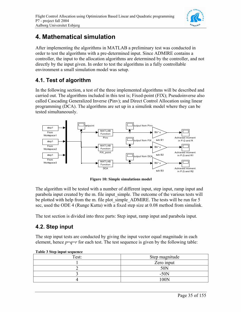
4.1. Test of algorithm In the following section, a test of the three implemented algorithms will be described and carried out. The algorithms included in this test is; Fixed-point (FIX); Pseudoinverse also called Cascading Generalized Inverse (Pinv); and Direct Control Allocation using linear programming (DCA). The algorithms are set up in a simulink model where they can be tested simultaneously.
Bb* u
sub B3
Bb* u
sub B2
Bb* u
sub B1
setpoint output from Pinv
output from FIX
output from DCA
MATLABFunction
Pinv
step1
FromWorkspace3
step1
FromWorkspace2
step1
FromWorkspace1
MATLABFunction
FIX_point
MATLABFunction
DCA Achieved moment in P,Q and R2
Achieved moment in P,Q and R1
Achieved moment in P,Q and R
Figure 10: Simple simulations model
The algorithm will be tested with a number of different input, step input, ramp input and parabola input created by the m. file input_simple. The outcome of the various tests will be plotted with help from the m. file plot_simple_ADMIRE. The tests will be run for 5 sec, used the ODE 4 (Runge Kutta) with a fixed step size at 0.08 method from simulink. The test section is divided into three parts: Step input, ramp input and parabola input.
4.2. Step input The step input tests are conducted by giving the input vector equal magnitude in each element, hence p=q=r for each test. The test sequence is given by the following table:
Table 3 Step input sequence Test: Step magnitude
1 Zero input 2 50N 3 -50N 4 100N
Page 35 of 155

Flight Control Allocation using Optimization Based Linear and Quadratic programming P7 - project fall 2004 Aalborg Universitet Esbjerg
5 -100N 6 200N 7 -200N 8 300N 9 -300N 10 400N 11 -400N
4.2.1. 1st test run, zero input
0 0.5 1 1.5 2 2.5 3 3.5 4 4.5 50
2
4
6x 10⁻⁴
Moment (N)
Desired moment P
PinvFIXDCADesired
0 0.5 1 1.5 2 2.5 3 3.5 4 4.5 5-0.08
-0.06
-0.04
-0.02
0
0.02
Moment (N)
Desired moment Q
PinvFIXDCADesired
0 0.5 1 1.5 2 2.5 3 3.5 4 4.5 5-15
-10
-5
0
5x 10⁻³
Time(sec)
Moment (N)
Desired moment R
PinvFIXDCADesired
Figure 11: 1st test run, desired moment and achieved moment
As it can be seen the input set point for P, Q, and R equals zero. The results from Pinv and DCA lies exactly on top of the curve representing the input signal. The achieved moment for FIX gives for P approximately 5.1 and for Q approximately -0.078 and last R approximately -13.5. This is not preferable because it commands the actuators to produce a moment which does not correspond the input.
Page 36 of 155

0 0.5 1 1.5 2 2.5 3 3.5 4 4.5 5-4
-2
0
Deflection(deg)
Deflection Right outer Elevon
PinvFIXDCA
0 0.5 1 1.5 2 2.5 3 3.5 4 4.5 5-6
-4
-2
0
Deflection(deg)
Deflection Right inner Elevon
PinvFIXDCA
0 0.5 1 1.5 2 2.5 3 3.5 4 4.5 5-4
-2
0
Deflection(deg)
Deflection Left outer Elevon
PinvFIXDCA
0 0.5 1 1.5 2 2.5 3 3.5 4 4.5 5-6
-4
-2
0
Time(sec)
Deflection(deg)
Deflection Left inner Elevon
PinvFIXDCA
Flight Control Allocation using Optimization Based Linear and Quadratic programming P7 - project fall 2004 Aalborg Universitet Esbjerg
Page 37 of 155
Figure 12: 1st test run, deflections for Right inner and outer elevon and Left inner and outer elevon
The graph in the top shows the desired deflection for the right outer elevon. As it can be seen the curves for Pinv and DCA tracks at zero. The curve for Fix lies at approximately -3.3. The second graph shows the desired deflection for the right inner elevon. The curves for Pinv and DCA again tracks zero. The curve for FIX follows at -5.4. A look at the last two graphs will reveal that they are identical with the two first. The moment produced differs from the commanded moment when using FIX, while both Pinv and DCA tracks the commanded moment properly.
0 0.5 1 1.5 2 2.5 3 3.5 4 4.5 5-15
-10
-5
0
Deflection(deg)
Deflection Left Canard
PinvFIXDCA
0 0.5 1 1.5 2 2.5 3 3.5 4 4.5 5-15
-10
-5
0
Deflection(deg)
Deflection Right Canard
PinvFIXDCA
0 0.5 1 1.5 2 2.5 3 3.5 4 4.5 50
2
4x 10⁻³
Time(sec)
Deflection(deg)
Deflection Rudder
PinvFIXDCA
Figure 13: 1st test run, deflections for Right and Left canard and the rudder

Flight Control Allocation using Optimization Based Linear and Quadratic programming P7 - project fall 2004 Aalborg Universitet Esbjerg The graph in the top shows the desired deflection for the left canard. As it can be seen both Pinv and DCA tracks at zero. The curve for FIX lies at approximately -11.5. The second graph shows the desired deflection for the left canard. Both Pinv and DCA tracks at zero. The curve for Fix lies at approximately -11.5. The bottom graph shows the desired deflection for the rudder. Pinv and DCA tracks at zero. The curve for FIX lies at approximately 0.0034.
1.1.1.1. Summary From this first test run it can be stated that the algorithm for Pinv and DCA tracks the desired input quite good. The FIX algorithm has an offset according to the desired input. The reason for this is that it in the start of the algorithm finds an initial start value. However, because there isn’t any contribution from the desired input, the outputs are set to the initial value. This property has the negative effect that it commands the actuators to produce some moment while zero moment is commanded.
Page 38 of 155

Flight Control Allocation using Optimization Based Linear and Quadratic programming P7 - project fall 2004 Aalborg Universitet Esbjerg
4.2.2. 2nd test run, step input
0 0.5 1 1.5 2 2.5 3 3.5 4 4.5 50
20
40
60
Moment (N)
Desired moment P
PinvFIXDCADesired
0 0.5 1 1.5 2 2.5 3 3.5 4 4.5 5-20
0
20
40
60
Moment (N)
Desired moment Q
PinvFIXDCADesired
0 0.5 1 1.5 2 2.5 3 3.5 4 4.5 5-20
0
20
40
60
Time(sec)
Moment (N)
Desired moment R
PinvFIXDCADesired
Figure 14: 2nd test run, desired moment and achieved moment
As it can be seen the input set point equals a step input of 50 at one sec. delay for P, Q, and R. The results from Pinv, DCA, and FIX lies on top of the commanded input and tracks it fine.
Page 39 of 155

0 0.5 1 1.5 2 2.5 3 3.5 4 4.5 5-6
-4
-2
0
Deflection(deg)
Deflection Right outer Elevon
PinvFIXDCA
0 0.5 1 1.5 2 2.5 3 3.5 4 4.5 5-10
-5
0
Deflection(deg)
Deflection Right inner Elevon
PinvFIXDCA
0 0.5 1 1.5 2 2.5 3 3.5 4 4.5 5-6
-4
-2
0
Deflection(deg)
Deflection Left outer Elevon
PinvFIXDCA
0 0.5 1 1.5 2 2.5 3 3.5 4 4.5 5-10
-5
0
5
Time(sec)
Deflection(deg)
Deflection Left inner Elevon
PinvFIXDCA
Flight Control Allocation using Optimization Based Linear and Quadratic programming P7 - project fall 2004 Aalborg Universitet Esbjerg
Page 40 of 155
Figure 15: 2nd test run, deflections for Right inner and outer elevon and Left inner and outer elevon The graph in the top shows the deflection for the right outer elevon. As it can be seen the curves goes for Pinv approximately to -2.4 and DCA goes to -4.6 after the step input. The curve for Fix goes approximately to -3.6 from an initial point at -3.3. The second graph shows the deflection for the right inner elevon. As it can be seen the curves for Pinv goes approximately to -4.2 and DCA goes to -4.6 after the step input. The curve for Fix goes approximately to -9.8 from an initial point at -5.3. The third graph shows the deflection for the left outer elevon. As it can be seen goes the curves for Pinv approximately to -0.4 and DCA goes to -4.6 after the step input. The curve for Fix goes approximately to -3.6 from an initial point at -3.3. The graph at the bottom shows the deflection for the left inner elevon. As it can be seen the curves stabilizes for Pinv around zero and DCA goes to 2 after the step input. The curve for Fix is almost stable at approximately -5.2.

0 0.5 1 1.5 2 2.5 3 3.5 4 4.5 5-20
-10
0
10
Deflection(deg)
Deflection Left Canard
PinvFIXDCA
0 0.5 1 1.5 2 2.5 3 3.5 4 4.5 5-20
-10
0
10
Deflection(deg)
Deflection Right Canard
PinvFIXDCA
0 0.5 1 1.5 2 2.5 3 3.5 4 4.5 5-10
-5
0
5
Time(sec)
Deflection(deg)
Deflection Rudder
PinvFIXDCA
Flight Control Allocation using Optimization Based Linear and Quadratic programming P7 - project fall 2004 Aalborg Universitet Esbjerg
Page 41 of 155
Figure 16: 2nd test run, deflection for Right and Left canard and the rudder
The graph in the top shows the deflection for the left canard. As it can be seen the curves for Pinv goes to 2.5 and DCA goes to 4. The curve for Fix goes approximately to -8.5 from an initial value at -12. The second graph shows the desired deflection for the left canard. As it can be seen the curves for Pinv goes to 0.5 and DCA goes to -4.4. The curve for Fix goes approximately to -11.4 from an initial value at -11.6. The bottom graph shows the desired deflection for the rudder. As it can be seen the curves for Pinv goes to -4.8 and DCA goes also to -4.8. The curve for FIX goes approximately to -6.2.

010
2030
4050
60
-10
0
10
20
30
40
50-10
0
10
20
30
40
50
Moment, P, (N)
Moment Directions
Moment, Q, (N)
Moment, R, (N)
PinvFIXDCADesired
Flight Control Allocation using Optimization Based Linear and Quadratic programming P7 - project fall 2004 Aalborg Universitet Esbjerg
Page 42 of 155
Figure 17: 2nd test run, the vector of moment shoving the direction of the desired and achieved moment
The above figure shows the tracking of the desired moment and its direction. And as it can be seen from the figure, all the other curves lie on top of each other and all algorithms track the desired moment fine.
1.1.1.2. Summary In this test run can it be seen that all three algorithms track the desired input moment. A look at the deflections of the control surfaces reveals that the deflections demanded by the FIX algorithm is lager then for the two other algorithms.

Flight Control Allocation using Optimization Based Linear and Quadratic programming P7 - project fall 2004 Aalborg Universitet Esbjerg
4.2.3. 3rd test run, step input
0 0.5 1 1.5 2 2.5 3 3.5 4 4.5 5-60
-40
-20
0
20
Moment (N)
Desired moment P
PinvFIXDCADesired
0 0.5 1 1.5 2 2.5 3 3.5 4 4.5 5-60
-40
-20
0
20
Moment (N)
Desired moment Q
PinvFIXDCADesired
0 0.5 1 1.5 2 2.5 3 3.5 4 4.5 5-60
-40
-20
0
20
Time(sec)
Moment (N)
Desired moment R
PinvFIXDCADesired
Figure 18: 3rd test run, desired moment and achieved moment
As it can be seen the input set point equals a step input of -50 at one sec. delay for P, Q, and R. The result from Pinv, DCA and FIX lies under the desired input and tracks it.
0 0.5 1 1.5 2 2.5 3 3.5 4 4.5 5-5
0
5
Deflection(deg)
Deflection Right outer Elevon
PinvFIXDCA
0 0.5 1 1.5 2 2.5 3 3.5 4 4.5 5-10
-5
0
5
Deflection(deg)
Deflection Right inner Elevon
PinvFIXDCA
0 0.5 1 1.5 2 2.5 3 3.5 4 4.5 5-5
0
5
Deflection(deg)
Deflection Left outer Elevon
PinvFIXDCA
0 0.5 1 1.5 2 2.5 3 3.5 4 4.5 5-10
-5
0
5
Time(sec)
Deflection(deg)
Deflection Left inner Elevon
PinvFIXDCA
Figure 19: 3rd test run, deflection for Right inner and outer elevon and Left inner and outer elevon
Page 43 of 155

Flight Control Allocation using Optimization Based Linear and Quadratic programming P7 - project fall 2004 Aalborg Universitet Esbjerg The graph in the top shows the deflection for the right outer elevon. As it can be seen the curves for Pinv goes approximately to 2.4 and DCA goes to 4.6 after the step input. The curve for Fix goes approximately to 1 from an initial point at -3.2. The second graph shows the deflection for the right inner elevon. As it can be seen the curves for Pinv goes approximately to 4.2 and DCA goes to 4.6 after the step input. The curve for Fix goes to approximately -1 from an initial point at -5.3. The third graph shows the deflection for the left outer elevon. As it can be seen the curves for Pinv goes approximately to -0.4 and DCA goes to -4 after the step input. The curve for Fix goes approximately to -3.3 from an initial point at -3.6. The bottom graph shows the deflection for the left inner elevon. As it can be seen is the curve for Pinv stable around zero and DCA goes to -3.3 after the entrees of the step. The curve for Fix is almost stable at approximately -5.2.
0 0.5 1 1.5 2 2.5 3 3.5 4 4.5 5-15
-10
-5
0
Deflection(deg)
Deflection Left Canard
PinvFIXDCA
0 0.5 1 1.5 2 2.5 3 3.5 4 4.5 5-20
-10
0
10
Deflection(deg)
Deflection Right Canard
PinvFIXDCA
0 0.5 1 1.5 2 2.5 3 3.5 4 4.5 50
5
10
Time(sec)
Deflection(deg)
Deflection Rudder
PinvFIXDCA
Figure 20: 3rd test run, deflection for Right and Left canard and the rudder
The graph at the top shows the deflection for the left canard. As it can be seen the curves for Pinv goes to -2.5 and DCA goes to 7.5. The curve for Fix goes approximately to -14 from an initial value at -12. The second graph shows the deflection for the left canard. As it can be seen the curves for Pinv goes to -0.5 and DCA goes to 3.5. The curve for Fix goes approximately to -11.6 from an initial value at -11.4. The bottom graph shows the deflection for the rudder. As it can be seen the curves for Pinv and DCA goes to 4. The curve for FIX goes approximately to 6.2.
Page 44 of 155

-60-50
-40-30
-20-10
010
-50
-40
-30
-20
-10
0
10-50
-40
-30
-20
-10
0
10
Moment, P, (N)
Moment Directions
Moment, Q, (N)
Moment, R, (N)
PinvFIXDCADesired
Flight Control Allocation using Optimization Based Linear and Quadratic programming P7 - project fall 2004 Aalborg Universitet Esbjerg
Page 45 of 155
Figure 21: 3rd test run, the vector of moment shoving the direction of the desired and achieved moment
The above figure shows the detection of the desired moment. And as it can be seen all the curves lie on top of each other.
1.1.1.3. Summary In this test run can it be seen that the entire three algorithm tracks the desired input moment. A look at the desired output deflection of the control surfaces can reveal that deflection demanded by the FIX algorithm is lager then for the two other algorithms.

Flight Control Allocation using Optimization Based Linear and Quadratic programming P7 - project fall 2004 Aalborg Universitet Esbjerg
4.2.4. 4th test run, step input
0 0.5 1 1.5 2 2.5 3 3.5 4 4.5 50
50
100
150
Moment(N)
Desired moment P
PinvFIXDCADesired
0 0.5 1 1.5 2 2.5 3 3.5 4 4.5 5-50
0
50
100
150
Moment(N)
Desired moment Q
PinvFIXDCADesired
0 0.5 1 1.5 2 2.5 3 3.5 4 4.5 5-50
0
50
100
Time(sec)
Moment(N)
Desired moment R
PinvFIXDCADesired
Figure 22: 4th test run, desired moment and achieved moment
As it can be seen the input set point equals a step input of 100 at one sec. delay for P, Q, and R. The result from Pinv, DCA and FIX lies under the desired input and tracks it fine.
Page 46 of 155

0 0.5 1 1.5 2 2.5 3 3.5 4 4.5 5-10
-5
0
Deflection(deg)
Deflection Right outer Elevon
PinvFIXDCA
0 0.5 1 1.5 2 2.5 3 3.5 4 4.5 5-15
-10
-5
0
Deflection(deg)
Deflection Right inner Elevon
PinvFIXDCA
0 0.5 1 1.5 2 2.5 3 3.5 4 4.5 5-10
-5
0
Deflection(deg)
Deflection Left outer Elevon
PinvFIXDCA
0 0.5 1 1.5 2 2.5 3 3.5 4 4.5 5-10
-5
0
5
Time(sec)
Deflection(deg)
Deflection Left inner Elevon
PinvFIXDCA
Flight Control Allocation using Optimization Based Linear and Quadratic programming P7 - project fall 2004 Aalborg Universitet Esbjerg
Page 47 of 155
Figure 23: 4th test run, deflection for Right inner and outer elevon and Left inner and outer elevon The graph at the top shows the deflection for the right outer elevon. As it can be seen the curves for Pinv goes approximately to -4.8 and DCA goes to -9.5 after the step input. The curve for Fix goes approximately to -8.1 from an initial point at -3.3. The second graph shows the deflection for the right inner elevon. As it can be seen the curves for Pinv goes approximately to -8 and DCA goes to -8.5 after the step input. The curve for Fix goes approximately to -14 from an initial point at -5.3. The third graph shows the deflection for the left outer elevon. As it can be seen the curves for Pinv goes approximately to -0.4 and DCA goes to -9.2 after the step input. The curve for Fix goes approximately to -4 from an initial point at -3.3. The bottom graph shows the deflection for the left inner elevon. As it can be seen the curves stabilizes for Pinv around zero and DCA goes to 4 after the step input. The curve for Fix is almost stable at approximately -5.2.

0 0.5 1 1.5 2 2.5 3 3.5 4 4.5 5-20
-10
0
10
Deflection(deg)
Deflection Left Canard
PinvFIXDCA
0 0.5 1 1.5 2 2.5 3 3.5 4 4.5 5-20
-10
0
10
Deflection(deg)
Deflection Right Canard
PinvFIXDCA
0 0.5 1 1.5 2 2.5 3 3.5 4 4.5 5-20
-10
0
10
Time(sec)
Deflection(deg)
Deflection Rudder
PinvFIXDCA
Flight Control Allocation using Optimization Based Linear and Quadratic programming P7 - project fall 2004 Aalborg Universitet Esbjerg
Page 48 of 155
Figure 24: 4th test run, deflection for Right and Left canard and the rudder
The top graph shows the deflection for the left canard. As it can be seen the curves for Pinv goes to 5.1 and DCA goes to 7.5. The curve for Fix goes approximately to -6.5 from an initial value at -12. The second graph shows the deflection for the left canard. As it can be seen the curves for Pinv goes to 0.5 and DCA goes to -9. The curve for Fix goes approximately to -11 from an initial value at -11.5. The bottom graph shows the deflection for the rudder. As it can be seen the curves for Pinv and DCA goes to -8. The curve for FIX goes approximately to -12.

020
4060
80100
120
-200
2040
6080
100120-20
0
20
40
60
80
100
120
Moment, P, (N)
Moment Directions
Moment, Q, (N)
MomenRN
PinvFIXDCADesired
Flight Control Allocation using Optimization Based Linear and Quadratic programming P7 - project fall 2004 Aalborg Universitet Esbjerg
Page 49 of 155
Figure 25: 4th test run, the vector of moment shoving the direction of the desired and achieved moment
The above figure shows the tracking of the desired moment. And as it can be seen all the curves lie on top of each other.
1.1.1.4. Summary In this test run can it be seen that the entire tree algorithm tracks the desired input moment. A look at the desired output deflection of the control surfaces can reveal that deflection demanded by the FIX algorithm is larger than for the two other algorithms.

Flight Control Allocation using Optimization Based Linear and Quadratic programming P7 - project fall 2004 Aalborg Universitet Esbjerg
4.2.5. 5th test run, step input
0 0.5 1 1.5 2 2.5 3 3.5 4 4.5 5-150
-100
-50
0
50
Moment (N)
Desired moment P
PinvFIXDCADesired
0 0.5 1 1.5 2 2.5 3 3.5 4 4.5 5-100
-50
0
50
Moment (N)
Desired moment Q
PinvFIXDCADesired
0 0.5 1 1.5 2 2.5 3 3.5 4 4.5 5-150
-100
-50
0
50
Time(sec)
Moment (N)
Desired moment R
PinvFIXDCADesired
Figure 26: 5th test run, desired moment and achieved moment
As it can be seen the input set point equals a step input of -100 at one sec. delay for P, Q, and R. The result from Pinv, DCA and FIX lies under the desired input and tracks it fine.
Page 50 of 155

0 0.5 1 1.5 2 2.5 3 3.5 4 4.5 5-5
0
5
10
Deflection(deg)
Deflection Right outer Elevon
PinvFIXDCA
0 0.5 1 1.5 2 2.5 3 3.5 4 4.5 5-10
0
10
Deflection(deg)
Deflection Right inner Elevon
PinvFIXDCA
0 0.5 1 1.5 2 2.5 3 3.5 4 4.5 5-5
0
5
10
Deflection(deg)
Deflection Left outer Elevon
PinvFIXDCA
0 0.5 1 1.5 2 2.5 3 3.5 4 4.5 5-10
-5
0
5
Time(sec)
Deflection(deg)
Deflection Left inner Elevon
PinvFIXDCA
Flight Control Allocation using Optimization Based Linear and Quadratic programming P7 - project fall 2004 Aalborg Universitet Esbjerg
Page 51 of 155
Figure 27: 5th test run, deflections for Right inner and outer elevon and Left inner and outer elevon The top graph shows the deflections for the right outer elevon. As it can be seen the curves for Pinv goes approximately to 4.8 and DCA goes to -7 after the step input. The curve for Fix goes approximately to 1.5 from an initial point at -3.3. The second graph shows the deflections for the right inner elevon. As it can be seen the curves for Pinv goes approximately to 8 and DCA goes to 7.5 after the step input. The curve for Fix goes approximately to 3.5 from an initial point at -5.3. The third graph shows the deflections for the left outer elevon. As it can be seen the curves for Pinv goes approximately to 0.4 and DCA goes to 8 after the step input. The curve for Fix goes approximately to -2.8 from an initial point at -3.3. The bottom graph shows the deflections for the left inner elevon. As it can be seen are the curves for Pinv stable around zero and DCA goes to -6.5 after the step input. The curve for Fix is almost stable at approximately -5.2.

0 0.5 1 1.5 2 2.5 3 3.5 4 4.5 5-20
-10
0
Deflection(deg)
Deflection Left Canard
PinvFIXDCA
0 0.5 1 1.5 2 2.5 3 3.5 4 4.5 5-20
-10
0
10
Deflection(deg)
Deflection Right Canard
PinvFIXDCA
0 0.5 1 1.5 2 2.5 3 3.5 4 4.5 50
5
10
15
Time(sec)
Deflection(deg)
Deflection Rudder
PinvFIXDCA
Flight Control Allocation using Optimization Based Linear and Quadratic programming P7 - project fall 2004 Aalborg Universitet Esbjerg
Page 52 of 155
Figure 28: 5th test run, deflections for Right and Left canard and the rudder
The top graph shows the deflections for the left canard. As it can be seen the curves for Pinv goes to -5.1 and DCA goes to -14.9. The curve for Fix goes approximately to -17 from an initial value at -12. The second graph shows the deflections for the left canard. As it can be seen the curves for Pinv goes to -0.5 and DCA goes to 7. The curve for Fix goes approximately to -12 from an initial value at -11. The third graph shows the deflections for the rudder. As it can be seen the curves for Pinv goes to 8 and DCA goes to also to 8. The curve for FIX goes approximately to 12.5.

-120-100
-80-60
-40-20
020
-100
-80
-60
-40
-20
0
20-120
-100
-80
-60
-40
-20
0
20
Moment, P, (N)
Moment Directions
Moment, Q, (N)
Moment, R, (N)
PinvFIXDCADesired
Flight Control Allocation using Optimization Based Linear and Quadratic programming P7 - project fall 2004 Aalborg Universitet Esbjerg
Figure 29: 5th test run, the vector of moment shoving the direction of the desired and achieved moment
The above figure shows the tracking of the desired moment. And as it can be seen all the curves lie on top of each other.
1.1.1.5. Summary In this test run can it be seen that all three algorithms track the desired input moment. A look at the desired output deflection of the control surfaces reveal that the deflections demanded by the FIX algorithm is larger than for the two other algorithms.
Page 53 of 155

Flight Control Allocation using Optimization Based Linear and Quadratic programming P7 - project fall 2004 Aalborg Universitet Esbjerg
4.2.6. 6th test run, step input
0 0.5 1 1.5 2 2.5 3 3.5 4 4.5 50
50
100
150
200
250
Moment (N)
Desired moment P
PinvFIXDCADesired
0 0.5 1 1.5 2 2.5 3 3.5 4 4.5 5-50
0
50
100
150
200
Moment (N)
Desired moment Q
PinvFIXDCADesired
0 0.5 1 1.5 2 2.5 3 3.5 4 4.5 5-50
0
50
100
150
200
Time(sec)
Moment (N)
Desired moment R
PinvFIXDCADesired
Figure 30: 6th test run, desired moment and achieved moment
As it can be seen the input set point equals a step input of 200 at one sec. delay for P, Q, and R. The result from Pinv, DCA and FIX lies under the desired input and tracks it fine.
0 0.5 1 1.5 2 2.5 3 3.5 4 4.5 5-20
-10
0
Deflection(deg)
Deflection Right outer Elevon
PinvFIXDCA
0 0.5 1 1.5 2 2.5 3 3.5 4 4.5 5-30
-20
-10
0
Deflection(deg)
Deflection Right inner Elevon
PinvFIXDCA
0 0.5 1 1.5 2 2.5 3 3.5 4 4.5 5-20
-10
0
Deflection(deg)
Deflection Left outer Elevon
PinvFIXDCA
0 0.5 1 1.5 2 2.5 3 3.5 4 4.5 5-10
0
10
Time(sec)
Deflection(deg)
Deflection Left inner Elevon
PinvFIXDCA
Figure 31: 6th test run, deflection for Right inner and outer elevon and Left inner and outer elevon
Page 54 of 155

Flight Control Allocation using Optimization Based Linear and Quadratic programming P7 - project fall 2004 Aalborg Universitet Esbjerg The top graph shows the deflection for the right outer elevon. As it can be seen the curves for Pinv goes approximately to -9.5 and DCA goes to -18 after the step input. The curve for Fix goes approximately to -14 from an initial point at -3.3. The second graph shows the deflection for the right inner elevon. As it can be seen the curves for Pinv goes approximately to -17.5 and DCA goes to -18 after the step input. The curve for Fix goes approximately to -23 from an initial point at -5.3. The third graph shows the deflection for the left outer elevon. As it can be seen the curves for Pinv goes approximately to -2 and DCA goes to -18 after the step input. The curve for Fix goes approximately to -4.8 from an initial point at -3.3. The bottom graph shows the deflection for then left inner elevon. As it can be seen the curves for Pinv stabilizes around zero and DCA goes to 8 after the step input. The curve for Fix is almost stable at approximately -5.2.
0 0.5 1 1.5 2 2.5 3 3.5 4 4.5 5-20
0
20
Deflection(deg)
Deflection Left Canard
PinvFIXDCA
0 0.5 1 1.5 2 2.5 3 3.5 4 4.5 5-20
-10
0
10
Deflection(deg)
Deflection Right Canard
PinvFIXDCA
0 0.5 1 1.5 2 2.5 3 3.5 4 4.5 5-40
-20
0
20
Time(sec)
Deflection(deg)
Deflection Rudder
PinvFIXDCA
Figure 32: 6th test run, deflection for Right and Left canard and the rudder
The top graph shows the deflection for the left canard. As it can be seen the curves for Pinv goes to 10.1 and DCA goes to 15.1. The curve for Fix goes approximately to -1 form an initial value at -12. The second graph shows the deflection for the left canard. As it can be seen the curves for Pinv goes to1.5 and DCA goes to -17.5. The curve for Fix goes approximately to -10.4 from an initial value at -12. The bottom graph shows the deflection for the rudder. As it can be seen the curves for Pinv goes to -18 and DCA goes to also to -18. The curve for FIX goes approximately to -25.
Page 55 of 155

050
100150
200250
-50
0
50
100
150
200-50
0
50
100
150
200
Moment, P, (N)
Moment Directions
Moment, Q, (N)
MomentR(N)
PinvFIXDCADesired
Flight Control Allocation using Optimization Based Linear and Quadratic programming P7 - project fall 2004 Aalborg Universitet Esbjerg
Page 56 of 155
Figure 33: 6th test run, the vector of moment shoving the direction of the desired and achieved moment
The above figure shows the tracking of the desired moment. And as it can be seen all the curves lie on top of each other.
1.1.1.6. Summary In this test run can it be seen that the entire three algorithm tracks the desired input moment. A look at the desired output deflection of the control surfaces can reveal that deflection demanded by the FIX algorithm is lager then for the two other algorithms.

Flight Control Allocation using Optimization Based Linear and Quadratic programming P7 - project fall 2004 Aalborg Universitet Esbjerg
4.2.7. 7th test run, step input
0 0.5 1 1.5 2 2.5 3 3.5 4 4.5 5-300
-200
-100
0
100Desired moment P
PinvFIXDCADesired
0 0.5 1 1.5 2 2.5 3 3.5 4 4.5 5-200
-150
-100
-50
0
50Desired moment Q
PinvFIXDCADesired
0 0.5 1 1.5 2 2.5 3 3.5 4 4.5 5-200
-150
-100
-50
0
50
Time(sec)
Desired moment R
PinvFIXDCADesired
Figure 34: 7th test run, desired moment and achieved moment
As it can be seen the input set point equals a step input of -200 at one sec. delay for P, Q, and R. The result from Pinv, DCA and FIX lies under the desired input and tracks it fine.
Page 57 of 155

0 0.5 1 1.5 2 2.5 3 3.5 4 4.5 5-10
0
10
20
Deflection(deg)
Deflection Right outer Elevon
PinvFIXDCA
0 0.5 1 1.5 2 2.5 3 3.5 4 4.5 5-10
0
10
20
Deflection(deg)
Deflection Right inner Elevon
PinvFIXDCA
0 0.5 1 1.5 2 2.5 3 3.5 4 4.5 5-10
0
10
20
Deflection(deg)
Deflection Left outer Elevon
PinvFIXDCA
0 0.5 1 1.5 2 2.5 3 3.5 4 4.5 5-20
-10
0
10
Time(sec)
Deflection(deg)
Deflection Left inner Elevon
PinvFIXDCA
Flight Control Allocation using Optimization Based Linear and Quadratic programming P7 - project fall 2004 Aalborg Universitet Esbjerg
Page 58 of 155
Figure 35: 7th test run, deflection for Right inner and outer elevon and Left inner and outer elevon
The top graph shows the deflection for the right outer elevon. As it can be seen the curves for Pinv goes approximately to 9.6 and DCA goes to 14 after the step input. The curve for Fix goes approximately to 6.5 from an initial point at -3.3. The second graph shows the deflection for the right inner elevon. As it can be seen the curves for Pinv goes approximately to 17.5 and DCA goes to 16 after the step input. The curve for Fix goes approximately to 12.5 from an initial point at -5.3. The third graph shows the deflection for the left outer elevon. As it can be seen the curves for Pinv goes approximately to 2 and DCA goes to 17 after the step input. The curve for Fix goes approximately to -2.3 from an initial point at -3.3. The bottom graph shows the deflection for the left inner elevon. As it can be seen the curves for Pinv stabilizes around zero and DCA goes to -13 after the step input. The curve for Fix is almost stable at approximately -5.2.

0 0.5 1 1.5 2 2.5 3 3.5 4 4.5 5-30
-20
-10
0
Deflection(deg)
Deflection Left Canard
PinvFIXDCA
0 0.5 1 1.5 2 2.5 3 3.5 4 4.5 5-20
0
20
Deflection(deg)
Deflection Right Canard
PinvFIXDCA
0 0.5 1 1.5 2 2.5 3 3.5 4 4.5 50
10
20
30
Time(sec)
Deflection(deg)
Deflection Rudder
PinvFIXDCA
Flight Control Allocation using Optimization Based Linear and Quadratic programming P7 - project fall 2004 Aalborg Universitet Esbjerg
Page 59 of 155
Figure 36: 7th test run, deflection for Right and Left canard and the rudder
The top graph shows the deflection for the left canard. As it can be seen the curves for Pinv goes to -10.1 and DCA goes to -29. The curve for Fix goes approximately to -1 form an initial value at -22. The second graph shows the deflection for the left canard. As it can be seen the curves for Pinv goes to -1.5 and DCA goes to 13.5. The curve for Fix goes approximately to -12.5 from an initial value at -11. The bottom graph shows the deflection for the rudder. As it can be seen the curves for Pinv and DCA goes to 17. The curve for FIX goes to at approximately 25.

-250-200
-150-100
-500
50
-200
-150
-100
-50
0
50-200
-150
-100
-50
0
50
Moment, P, (N)
Moment Directions
Moment, Q, (N)
Moment, R, (N)
PinvFIXDCADesired
Flight Control Allocation using Optimization Based Linear and Quadratic programming P7 - project fall 2004 Aalborg Universitet Esbjerg
Page 60 of 155
Figure 37: 7th test run, the vector of moment shoving the direction of the desired and achieved moment
The above figure shows the tracking of the desired moment. And as it can be seen all the curves lie on top of each other.
4.2.8. Summary In this test run can it be seen that all three algorithm track the desired input moment. A look at the desired output deflection of the control surfaces can reveal that deflection demanded by the FIX algorithm is larger than for the two other algorithms.

Flight Control Allocation using Optimization Based Linear and Quadratic programming P7 - project fall 2004 Aalborg Universitet Esbjerg
4.2.9. 8th test run step input
0 0.5 1 1.5 2 2.5 3 3.5 4 4.5 5-200
0
200
400
Moment (N)
Desired moment P
PinvFIXDCADesired
0 0.5 1 1.5 2 2.5 3 3.5 4 4.5 5-100
0
100
200
300
400
Moment (N)
Desired moment Q
PinvFIXDCADesired
0 0.5 1 1.5 2 2.5 3 3.5 4 4.5 5-100
0
100
200
300
400
Time(sec)
Moment (N)
Desired moment R
PinvFIXDCADesired
Figure 38: 8th test run, desired moment and achieved moment
As it can be seen the input set point equals a step input of 300 at one sec. delay for P, Q, and R. In the top graph, the curve for Pinv goes approximately to -190, and the curve for DCA goes approximately to 300 and the curve for FIX lays under the curve for DCA. In the middle graph, the curve for Pinv goes approximately to 250, and the curve for DCA goes approximately to 300 and the curve for FIX lays under the curve for DCA. In the bottom graph, the curve for Pinv goes approximately to 160, and the curve for DCA goes approximately to 300 and the curve for FIX lays nearly under the curve for DCA.
Page 61 of 155

0 0.5 1 1.5 2 2.5 3 3.5 4 4.5 5-50
0
50
Deflection(deg)
Deflection Right outer Elevon
PinvFIXDCA
0 0.5 1 1.5 2 2.5 3 3.5 4 4.5 5-30
-20
-10
0
Deflection(deg)
Deflection Right inner Elevon
PinvFIXDCA
0 0.5 1 1.5 2 2.5 3 3.5 4 4.5 5-50
0
50
Deflection(deg)
Deflection Left outer Elevon
PinvFIXDCA
0 0.5 1 1.5 2 2.5 3 3.5 4 4.5 5-40
-20
0
20
Time(sec)
Deflection(deg)
Deflection Left inner Elevon
PinvFIXDCA
Flight Control Allocation using Optimization Based Linear and Quadratic programming P7 - project fall 2004 Aalborg Universitet Esbjerg
Page 62 of 155
Figure 39: 8th test run, deflection for Right inner and outer elevon and Left inner and outer elevon The top graph shows the deflection for the right outer elevon. As it can be seen the curves for Pinv goes approximately to 30 (saturated) and DCA goes to -28 after the step input. The curve for Fix goes to -19 from an initial point at -3.3. The second graph shows the desired deflection for the right inner elevon. As it can be seen the curves for Pinv goes approximately to -26 and DCA goes to -26 after the step input. The curve for Fix goes to -30 (saturated) from an initial point at -5.3. The third graph shows the deflection for the left outer elevon. As it can be seen the curves for Pinv goes approximately to 30 (saturated) and DCA goes to -28 after the step input. The curve for Fix goes approximately -28 from an initial point at -3.3. The bottom graph shows the deflection for the left inner elevon. As it can be seen the curves for Pinv goes to -30 (saturated) and DCA goes to 12 after the step input. The curve for Fix goes to 2.5 from the initial point -5.3.
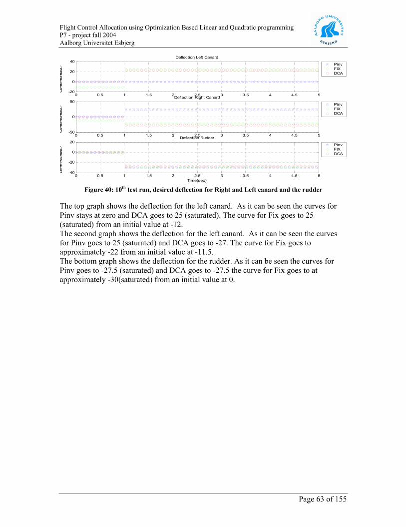
0 0.5 1 1.5 2 2.5 3 3.5 4 4.5 5-20
0
20
40
Deflection(deg)
Deflection Left Canard
PinvFIXDCA
0 0.5 1 1.5 2 2.5 3 3.5 4 4.5 5-50
0
50
Deflection(deg)
Deflection Right Canard
PinvFIXDCA
0 0.5 1 1.5 2 2.5 3 3.5 4 4.5 5-40
-20
0
20
Time(sec)
Deflection(deg)
Deflection Rudder
PinvFIXDCA
Flight Control Allocation using Optimization Based Linear and Quadratic programming P7 - project fall 2004 Aalborg Universitet Esbjerg
Page 63 of 155
Figure 40: 10th test run, desired deflection for Right and Left canard and the rudder
The top graph shows the deflection for the left canard. As it can be seen the curves for Pinv stays at zero and DCA goes to 25 (saturated). The curve for Fix goes to 25 (saturated) from an initial value at -12. The second graph shows the deflection for the left canard. As it can be seen the curves for Pinv goes to 25 (saturated) and DCA goes to -27. The curve for Fix goes to approximately -22 from an initial value at -11.5. The bottom graph shows the deflection for the rudder. As it can be seen the curves for Pinv goes to -27.5 (saturated) and DCA goes to -27.5 the curve for Fix goes to at approximately -30(saturated) from an initial value at 0.

-200-100
0100
200300
400
-100
0
100
200
300-50
0
50
100
150
200
250
300
350
Moment, P, (N)
Moment Directions
Moment, Q, (N)
MomentR(N)
PinvFIXDCADesired
Flight Control Allocation using Optimization Based Linear and Quadratic programming P7 - project fall 2004 Aalborg Universitet Esbjerg
Page 64 of 155
Figure 41: 10th test run, the vector of moment shoving the direction of the desired and achieved moment
The above figure shows the tracking of the desired moment. The curves for Pinv can not track the desired moment direction. DCA and FIX tracks the desired moment direction quite good.
1.1.1.7. Summary In this test run can it be seen that only the FIX and DCA algorithms track the desired input moment. The Pinv algorithm can’t track the desired input. The Pinv algorithm also produces a wrong direction of the moment generated by the control surface deflections.
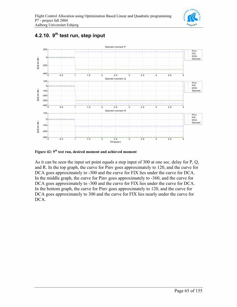
Flight Control Allocation using Optimization Based Linear and Quadratic programming P7 - project fall 2004 Aalborg Universitet Esbjerg
4.2.10. 9th test run, step input
0 0.5 1 1.5 2 2.5 3 3.5 4 4.5 5-400
-200
0
200
Moment (N)
Desired moment P
PinvFIXDCADesired
0 0.5 1 1.5 2 2.5 3 3.5 4 4.5 5-400
-300
-200
-100
0
100
Moment (N)
Desired moment Q
PinvFIXDCADesired
0 0.5 1 1.5 2 2.5 3 3.5 4 4.5 5-300
-200
-100
0
100
Time(sec)
Moment (N)
Desired moment R
PinvFIXDCADesired
Figure 42: 9th test run, desired moment and achieved moment As it can be seen the input set point equals a step input of 300 at one sec. delay for P, Q, and R. In the top graph, the curve for Pinv goes approximately to 120, and the curve for DCA goes approximately to -300 and the curve for FIX lies under the curve for DCA. In the middle graph, the curve for Pinv goes approximately to -360, and the curve for DCA goes approximately to -300 and the curve for FIX lies under the curve for DCA. In the bottom graph, the curve for Pinv goes approximately to 120, and the curve for DCA goes approximately to 300 and the curve for FIX lies nearly under the curve for DCA.
Page 65 of 155

0 0.5 1 1.5 2 2.5 3 3.5 4 4.5 5-50
0
50
Deflection(deg)
Deflection Right outer Elevon
PinvFIXDCA
0 0.5 1 1.5 2 2.5 3 3.5 4 4.5 5-20
0
20
40
Deflection(deg)
Deflection Right inner Elevon
PinvFIXDCA
0 0.5 1 1.5 2 2.5 3 3.5 4 4.5 5-50
0
50
Deflection(deg)
Deflection Left outer Elevon
PinvFIXDCA
0 0.5 1 1.5 2 2.5 3 3.5 4 4.5 5-20
0
20
40
Time(sec)
Deflection(deg)
Deflection Left inner Elevon
PinvFIXDCA
Flight Control Allocation using Optimization Based Linear and Quadratic programming P7 - project fall 2004 Aalborg Universitet Esbjerg
Page 66 of 155
Figure 43: 9th test run, deflection for Right inner and outer elevon and Left inner and outer elevon The top graph shows the deflection for the right outer elevon. As it can be seen the curves for Pinv goes approximately to -30 (saturated) and DCA goes to 21 after the step input. The curve for Fix goes to 5 from an initial point at -3.3. The second graph shows the deflection for the right inner elevon. As it can be seen the curves for Pinv goes approximately to 30 (saturated) and DCA goes to 24 after the step input. The curve for Fix goes to 28 from an initial point at -5.3. The third graph shows the deflection for the left outer elevon. As it can be seen the curves for Pinv goes approximately to -30 (saturated) and DCA goes to 24 after the step input. The curve for Fix goes approximately to 5 from an initial point at -3.3. The bottom graph shows the deflection for the left inner elevon. As it can be seen the curves for Pinv goes to 30 (saturated) and DCA goes to -19 after the step input. The curve for Fix goes to -12.5 from the initial point -5.3

0 0.5 1 1.5 2 2.5 3 3.5 4 4.5 5-50
0
50
Deflection(deg)
Deflection Left Canard
PinvFIXDCA
0 0.5 1 1.5 2 2.5 3 3.5 4 4.5 5-100
-50
0
50Deflection Right Canard
PinvFIXDCA
0 0.5 1 1.5 2 2.5 3 3.5 4 4.5 50
10
20
30
Time(sec)
Deflection(deg)
Deflection Rudder
PinvFIXDCA
Flight Control Allocation using Optimization Based Linear and Quadratic programming P7 - project fall 2004 Aalborg Universitet Esbjerg
Page 67 of 155
Figure 44: 9th test run, deflection for Right and Left canard and the rudder
The top graph shows the deflection for the left canard. As it can be seen the curves for Pinv stays around zero and DCA goes to -50. The curve for Fix goes to -40 from an initial value at -12. The second graph shows the deflection for the left canard. As it can be seen the curves for Pinv goes to -55 (saturated) and DCA goes to 20. The curve for Fix goes approximately to 0 from an initial value at -11.5. The bottom graph shows the deflection for the rudder. As it can be seen the curves for Pinv goes to 30 (saturated) and DCA goes to -24. The curve for Fix goes to at approximately -30(saturated) from an initial value at 0.

-400-300
-200-100
0100
200
-400
-300
-200
-100
0
100-300
-250
-200
-150
-100
-50
0
50
Moment, P, (N)
Moment Directions
Moment, Q, (N)
Moment, R, (N)
PinvFIXDCADesired
Flight Control Allocation using Optimization Based Linear and Quadratic programming P7 - project fall 2004 Aalborg Universitet Esbjerg
Page 68 of 155
Figure 45: 9th test run, the vector of moment shoving the direction of the desired and achieved moment
The above figure shows the detection of the desired moment. The curves for Pinv can not track the desired moment direction. DCA and FIX tracks the desired moment direction quite good.
1.1.1.8. Summary In this test run it can be seen that only the algorithm for FIX and DCA tracks the desired input moment. The Pinv algorithm can’t track the desired input. Many actuators reach saturation when using the Pinv algorithm, hence it becomes difficult to keep directionality. The direction of the moment for Pinv algorithm is off track.

Flight Control Allocation using Optimization Based Linear and Quadratic programming P7 - project fall 2004 Aalborg Universitet Esbjerg
4.2.11. 10th test run, step input
0 0.5 1 1.5 2 2.5 3 3.5 4 4.5 5-200
0
200
400
Moment (N)
Desired moment P
PinvFIXDCADesired
0 0.5 1 1.5 2 2.5 3 3.5 4 4.5 5-100
0
100
200
300
400
Moment (N)
Desired moment Q
PinvFIXDCADesired
0 0.5 1 1.5 2 2.5 3 3.5 4 4.5 5-100
0
100
200
300
400
Time(sec)
Moment (N)
Desired moment R
PinvFIXDCADesired
Figure 46: 10th test run, desired moment and achieved moment
As it can be seen the input set point equals a step input of 400 at one sec. delay for P, Q, and R. In the top graph, the curve for Pinv goes approximately to -180, and the curve for DCA goes approximately to 320 and the curve for FIX lies under the curve for DCA. In the middle graph, the curve for Pinv goes approximately to 250, and the curve for DCA goes approximately to 320 and the curve for FIX goes approximately to 370. In the bottom graph, the curve for Pinv goes approximately to 160, and the curve for DCA goes approximately to 320 and the curve for FIX goes approximately to 330. As it can be seen, none of the achieved moments track the desired moments.
Page 69 of 155

0 0.5 1 1.5 2 2.5 3 3.5 4 4.5 5-50
0
50
Deflection(deg)
Deflection Right outer Elevon
PinvFIXDCA
0 0.5 1 1.5 2 2.5 3 3.5 4 4.5 5-30
-20
-10
0
Deflection(deg)
Deflection Right inner Elevon
PinvFIXDCA
0 0.5 1 1.5 2 2.5 3 3.5 4 4.5 5-50
0
50
Deflection(deg)
Deflection Left outer Elevon
PinvFIXDCA
0 0.5 1 1.5 2 2.5 3 3.5 4 4.5 5-40
-20
0
20
Time(sec)
Deflection(deg)
Deflection Left inner Elevon
PinvFIXDCA
Flight Control Allocation using Optimization Based Linear and Quadratic programming P7 - project fall 2004 Aalborg Universitet Esbjerg
Page 70 of 155
Figure 47: 10th test run, deflection for Right inner and outer elevon and Left inner and outer elevon
The top graph shows the deflection for then right outer elevon. As it can be seen the curves for Pinv goes approximately to 30 (saturated) and DCA goes to -30 (saturated) after the step input. The curve for Fix goes to -30 (saturated) from an initial point at -3.3. The second graph shows the deflection for then right inner elevon. As it can be seen the curves for Pinv goes approximately to -30 (saturated) and DCA goes to -30 (saturated) after the step input. The curve for Fix goes to -30 (saturated) from an initial point at -5.3. The third graph shows the deflection for then left outer elevon. As it can be seen the curves for Pinv goes approximately to 30 (saturated) and DCA goes to -30 (saturated) after the step input. The curve for Fix goes approximately to -28 from an initial point at -3.3. The bottom graph shows the deflection for then left inner elevon. As it can be seen the curves for Pinv goes to -30 (saturated) and DCA goes to 13 after the step input. The curve for Fix goes to 15 from the initial point -5.3.

0 0.5 1 1.5 2 2.5 3 3.5 4 4.5 5-20
0
20
40
Deflection(deg)
Deflection Left Canard
PinvFIXDCA
0 0.5 1 1.5 2 2.5 3 3.5 4 4.5 5-50
0
50
Deflection(deg)
Deflection Right Canard
PinvFIXDCA
0 0.5 1 1.5 2 2.5 3 3.5 4 4.5 5-40
-20
0
20
Time(sec)
Deflection(deg)
Deflection Rudder
PinvFIXDCA
Flight Control Allocation using Optimization Based Linear and Quadratic programming P7 - project fall 2004 Aalborg Universitet Esbjerg
Page 71 of 155
Figure 48: 10th test run, deflection for Right and Left canard and the rudder
The top graph shows the deflection for the left canard. As it can be seen the curves for Pinv stays around zero and DCA goes to 25 (saturated). The curve for Fix goes to 25 (saturated) from an initial value at -12. The second graph shows the deflection for the left canard. As it can be seen the curves for Pinv goes to 25 (saturated) and DCA goes to -28. The curve for Fix goes approximately to -12.5 from an initial value at -11. The bottom graph shows the deflection for the rudder. As it can be seen all the curves go to -30 (saturated).
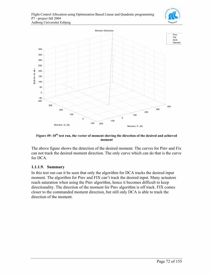
-200-100
0100
200300
400
-100
0
100
200
300
400-50
0
50
100
150
200
250
300
350
400
Moment, P, (N)
Moment Directions
Moment, Q, (N)
Moment, R, (N)
PinvFIXDCADesired
Flight Control Allocation using Optimization Based Linear and Quadratic programming P7 - project fall 2004 Aalborg Universitet Esbjerg
Page 72 of 155
Figure 49: 10th test run, the vector of moment shoving the direction of the desired and achieved moment
The above figure shows the detection of the desired moment. The curves for Pinv and Fix can not track the desired moment direction. The only curve which can do that is the curve for DCA.
1.1.1.9. Summary In this test run can it be seen that only the algorithm for DCA tracks the desired input moment. The algorithm for Pinv and FIX can’t track the desired input. Many actuators reach saturation when using the Pinv algorithm, hence it becomes difficult to keep directionality. The direction of the moment for Pinv algorithm is off track. FIX comes closer to the commanded moment direction, but still only DCA is able to track the direction of the moment.

Flight Control Allocation using Optimization Based Linear and Quadratic programming P7 - project fall 2004 Aalborg Universitet Esbjerg
1.1.1.10. 11th test run, step input
0 0.5 1 1.5 2 2.5 3 3.5 4 4.5 5-600
-400
-200
0
200
400
Moment (N)
Desired moment P
PinvFIXDCADesired
0 0.5 1 1.5 2 2.5 3 3.5 4 4.5 5-400
-300
-200
-100
0
100
Moment (N)
Desired moment Q
PinvFIXDCADesired
0 0.5 1 1.5 2 2.5 3 3.5 4 4.5 5-400
-300
-200
-100
0
100
Time(sec)
Moment (N)
Desired moment R
PinvFIXDCADesired
Figure 50: 11th test run, desired moment and achieved moment
As it can be seen the input set point equals a step input of -400 at one sec. delay for P, Q, and R. In the top graph, the curve for Pinv goes approximately to 210, and the curve for DCA goes approximately to -360 and the curve for FIX lies under the curve for DCA. In the middle graph, the curve for Pinv goes approximately to -150, and the curve for DCA goes approximately to -360 and the curve for FIX goes approximately to -390. In the bottom graph, the curve for Pinv goes approximately to -180, and the curve for DCA goes approximately to -360 and the curve for FIX goes approximately to -360. As it can be seen none of the achieved moments track the desired moments.
Page 73 of 155

0 0.5 1 1.5 2 2.5 3 3.5 4 4.5 5-50
0
50
Deflection(deg)
Deflection Right outer Elevon
PinvFIXDCA
0 0.5 1 1.5 2 2.5 3 3.5 4 4.5 5-20
0
20
40
Deflection(deg)
Deflection Right inner Elevon
PinvFIXDCA
0 0.5 1 1.5 2 2.5 3 3.5 4 4.5 5-50
0
50
Deflection(deg)
Deflection Left outer Elevon
PinvFIXDCA
0 0.5 1 1.5 2 2.5 3 3.5 4 4.5 5-50
0
50
Time(sec)
Deflection(deg)
Deflection Left inner Elevon
PinvFIXDCA
Flight Control Allocation using Optimization Based Linear and Quadratic programming P7 - project fall 2004 Aalborg Universitet Esbjerg
Page 74 of 155
Figure 51: 11th test run, deflection for Right inner and outer elevon and Left inner and outer elevon The top graph shows the deflection for the right outer elevon. As it can be seen the curves for Pinv goes approximately to -30 (saturated) and DCA goes to 25 after the step input. The curve for Fix goes to 29 from an initial point at -3.3. The second graph shows the deflection for the right inner elevon. As it can be seen the curves for Pinv goes approximately to 30 (saturated) and DCA goes to 30 (saturated) after the step input. The curve for Fix goes to 30 (saturated) from an initial point at -5.3. The third graph shows the deflection for the left outer elevon. As it can be seen the curves for Pinv goes approximately to -30 (saturated) and DCA goes to 30 (saturated) after the step input. The curve for Fix goes approximately to 30 (saturated) from an initial point at -3.3. The bottom graph shows the deflection for the left inner elevon. As it can be seen the curves for Pinv goes to 30 (saturated) and DCA goes to -24 after the step input. The curve for Fix goes to -22 from the initial point -5.3.

0 0.5 1 1.5 2 2.5 3 3.5 4 4.5 5-100
-50
0
50Deflection Left Canard
PinvFIXDCA
0 0.5 1 1.5 2 2.5 3 3.5 4 4.5 5-20
0
20
40
Deflection(deg)
Deflection Right Canard
PinvFIXDCA
0 0.5 1 1.5 2 2.5 3 3.5 4 4.5 50
10
20
30
Time(sec)
Deflection(deg)
Deflection Rudder
PinvFIXDCA
Flight Control Allocation using Optimization Based Linear and Quadratic programming P7 - project fall 2004 Aalborg Universitet Esbjerg
Page 75 of 155
Figure 52: 11th test run, deflection for Right and Left canard and the rudder
The top graph shows the deflection for the left canard. As it can be seen the curves for Pinv stays around zero and DCA goes to -55 (saturated). The curve for Fix goes to -55 (saturated) from an initial value at -12. The second graph shows the deflection for the left canard. As it can be seen the curves for Pinv stays around zero and DCA goes to 25 (saturated). The curve for Fix goes approximately to 22.5 from an initial value at -11.5. The bottom graph shows the deflection for the rudder. As it can be seen all the curves go to 30 (saturated).

-500-400
-300-200
-1000
100200
300
-400
-300
-200
-100
0
100-400
-350
-300
-250
-200
-150
-100
-50
0
50
Moment, P, (N)
Moment Directions
Moment, Q, (N)
Moment, R, (N)
PinvFIXDCADesired
Flight Control Allocation using Optimization Based Linear and Quadratic programming P7 - project fall 2004 Aalborg Universitet Esbjerg
Page 76 of 155
Figure 53: 9th test run, the vector of moment shoving the direction of the desired and achieved moment
The above figure shows the detection of the desired moment. The curves for Pinv can not track the desired moment direction. DCA and FIX tracks the desired moment direction quite good.
1.1.1.11. Summary In this test run can it be seen that only the algorithm for FIX and DCA tracks the desired input moment. The algorithm for Pinv can’t track the desired input. Many actuators reach saturation when using the Pinv algorithm, hence it becomes difficult to keep directionality. The direction of the moment for Pinv algorithm is off track. Both FIX and DCA is able to track the direction of the moment.
4.3. Ramp input The ramp input tests are conducted by giving the input vector equal magnitude in each element, hence p=q=r for each test. The test sequence is given by the following table:
Table 4 Ramp input sequence Test: Slope
12 100N/second 13 -100N/second

Flight Control Allocation using Optimization Based Linear and Quadratic programming P7 - project fall 2004 Aalborg Universitet Esbjerg
4.3.1. 12th test run, ramp input.
0 0.5 1 1.5 2 2.5 3 3.5 4 4.5 5-400
-200
0
200
400
Moment (N)
Desired moment P
PinvFIXDCADesired
0 0.5 1 1.5 2 2.5 3 3.5 4 4.5 5-100
0
100
200
300
400
Moment (N)
Desired moment Q
PinvFIXDCADesired
0 0.5 1 1.5 2 2.5 3 3.5 4 4.5 5-100
0
100
200
300
400
Time(sec)
Moment (N)
Desired moment R
PinvFIXDCADesired
Figure 54: 12th test run, desired moment and achieved moment
As it can be seen the input set point equals a ramp input with a slope of 100 units per second for P, Q, and R. In the top graph, the curve for Pinv follows the desired moment until it reaches 290 where it drops to approximately -190. Here it stays until the desired input reaches 440 where the curve for Pinv goes to 580 where it stops. For DCA the curve tracks the ramp input up to approximately 310, where it clips the moment generation. The curve for FIX keeps on tracking the desired input. In the middle graph, the curve for Pinv follows the desired moment until it reaches 290, here it drops to approximately 180, and shortly afterwards it rises a little, approximately to 230. It stays at this value until the desired input reaches 440, where the curve for Pinv goes down in two steps until it reaches 10. The curve for DCA goes approximately to 310. The curve for FIX follows the desired input until it reaches 270 where it clips the moment generation and falls a little back. In the bottom graph, the curve for Pinv follows the desired moment until it reaches 290, here it drops to approximately 180, where it stays until the desired input reaches 440 where the curve for Pinv goes up to 400 shortly and the settles at approximately 380. FIX and DCA tracks the desired input until it reaches 310, at this point it almost settles.
Page 77 of 155

0 0.5 1 1.5 2 2.5 3 3.5 4 4.5 5-50
0
50
Deflection(deg)
Deflection Right outer Elevon
PinvFIXDCA
0 0.5 1 1.5 2 2.5 3 3.5 4 4.5 5-30
-20
-10
0
Deflection(deg)
Deflection Right inner Elevon
PinvFIXDCA
0 0.5 1 1.5 2 2.5 3 3.5 4 4.5 5-50
0
50
Deflection(deg)
Deflection Left outer Elevon
PinvFIXDCA
0 0.5 1 1.5 2 2.5 3 3.5 4 4.5 5-40
-20
0
20
Time(sec)
Deflection(deg)
Deflection Left inner Elevon
PinvFIXDCA
Flight Control Allocation using Optimization Based Linear and Quadratic programming P7 - project fall 2004 Aalborg Universitet Esbjerg
Page 78 of 155
Figure 55: 14th test run, deflection for Right inner and outer elevon and Left inner and outer elevon
The top graph shows the deflection for the right outer elevon. At the start the Pinv curve drops by 5 per sec until it reaches -12.5. at this point it start rising at 5 per sec. at the mark 2.8 sec the curve rises to 30 (saturated) here it settles until mark 4.6 sec. At this time point it drops to -30 (saturated). DCA drops following a slope given by -9 per sec. until it reaches -30 (saturated). FIX starts at -3.3 and drops to -30. The second graph shows the deflection for the right inner elevon. The curves for Pinv and DCA drops along a -11 per sec. slope until it reaches -30 (saturated). The curve for FIX drops along the same slope but it reaches -30 (saturated) approximately a half sec. before the two other curves. The reason for this is that it starts from an initial position of -5.6. The third graph shows the deflection for the left outer elevon. A look at the curve for Pinv shows that there is not much activity before mark 2.5 sec. after this mark the curve drops to -5 and shortly after rises to 30 (saturated). Here it settles until the 4.6 sec mark where it drops to -30 (saturated). Here it settles. The curve for FIX doesn’t change much before the 2.5 sec mark. After this point it drops to -30 (saturated) over a 1.5sec period. The curve for DCA drops from zero to -30 (saturated) over a period of 3.2 sec where it settles. The bottom graph shows the deflection for the left inner elevon. The curve for Pinv is settled at zero at until 2.5 sec mark, at this mark raises the curve slightly until 5 and then drops to -30 (saturated). At the 2.8 sec mark the curve settles until the 4.6 sec mark where it reaches to 30 (saturated). At this point it settles. The curve for FIX is stabilized at -5.6 until the 2.5 sec mark. After this point it raises to 20 over 2.5 sec. the curve for DCA rises over 3.2 sec to 12 where it settles.

0 0.5 1 1.5 2 2.5 3 3.5 4 4.5 5-20
0
20
40
Deflection(deg)
Deflection Left Canard
PinvFIXDCA
0 0.5 1 1.5 2 2.5 3 3.5 4 4.5 5-50
0
50
Deflection(deg)
Deflection Right Canard
PinvFIXDCA
0 0.5 1 1.5 2 2.5 3 3.5 4 4.5 5-40
-20
0
20
Time(sec)
Deflection(deg)
Deflection Rudder
PinvFIXDCA
Flight Control Allocation using Optimization Based Linear and Quadratic programming P7 - project fall 2004 Aalborg Universitet Esbjerg
Page 79 of 155
Figure 56: 12th test run, desired deflection for Right and Left canard and the rudder
The top graph shows the deflection for the left canard. The Pinv curve has some huge fluctuations over time and finally settles at zero deflection. DCA goes to 25 (saturated). The curve for Fix goes also to 25 (saturated) from an initial value at -12. The second graph shows the deflection for the left canard. The Pinv curve has some huge fluctuations along with time and ends out at -55 (saturated). DCA goes to -30 and settles at 3.2sec mark. The curve for Fix makes a drop to -30 and the goes to 10 from an initial value at -11.5. The bottom graph shows the deflection for the rudder. As it can be seen goes the curves for Pinv, FIX and DCA all to 30 (saturated), the curve for Pinv and FIX at the 2.4 sec mark and the curve for DCA at 3.3 sec mark.

-400-200
0200
400600
-100
0
100
200
300
400
500-100
0
100
200
300
400
500
Moment, P, (N)
Moment Directions
Moment, Q, (N)
Moment, R, (N)
PinvFIXDCADesired
Flight Control Allocation using Optimization Based Linear and Quadratic programming P7 - project fall 2004 Aalborg Universitet Esbjerg
Page 80 of 155
Figure 57: 14th test run, the vector of moment shoving the direction of the desired and achieved moment
The above figure shows the detection of the desired moment. The curves for Pinv and FIX can not track the desired moment direction. DCA tracks the desired moment direction quite good.
1.1.1.12. Summary In this test run it can be seen that only the algorithm for DCA tracks the desired input moment. The algorithm for Pinv and FIX can’t track the desired input. The reason for this is that both algorithms has problems when they violate the constraints. DCA scales its output vector, and preserves directionality while both FIX and Pinv attempts to keep up with the moment demand.
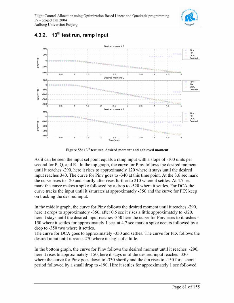
Flight Control Allocation using Optimization Based Linear and Quadratic programming P7 - project fall 2004 Aalborg Universitet Esbjerg
4.3.2. 13th test run, ramp input
0 0.5 1 1.5 2 2.5 3 3.5 4 4.5 5-400
-200
0
200
400
Moment (N)
Desired moment P
PinvFIXDCADesired
0 0.5 1 1.5 2 2.5 3 3.5 4 4.5 5-400
-300
-200
-100
0
100
Moment (N)
Desired moment Q
PinvFIXDCADesired
0 0.5 1 1.5 2 2.5 3 3.5 4 4.5 5-400
-300
-200
-100
0
100
Time(sec)
Moment (N)
Desired moment R
PinvFIXDCADesired
Figure 58: 13th test run, desired moment and achieved moment
As it can be seen the input set point equals a ramp input with a slope of -100 units per second for P, Q, and R. In the top graph, the curve for Pinv follows the desired moment until it reaches -290, here it rises to approximately 120 where it stays until the desired input reaches 340. The curve for Pinv goes to -340 at this time point. At the 3.6 sec mark the curve rises to 120 and shortly after rises further to 210 where it settles. At 4.7 sec mark the curve makes a spike followed by a drop to -520 where it settles. For DCA the curve tracks the input until it saturates at approximately -350 and the curve for FIX keep on tracking the desired input. In the middle graph, the curve for Pinv follows the desired moment until it reaches -290, here it drops to approximately -350, after 0.5 sec it rises a little approximately to -320. here it stays until the desired input reaches -350 here the curve for Pinv rises to it rashes -150 where it settles for approximately 1 sec. at 4.7 sec mark a spike occurs followed by a drop to -350 two where it settles. The curve for DCA goes to approximately -350 and settles. The curve for FIX follows the desired input until it reacts 270 where it slag’s of a little. In the bottom graph, the curve for Pinv follows the desired moment until it reaches -290, here it rises to approximately -150, here it stays until the desired input reaches -330 where the curve for Pinv goes dawn to -330 shortly and the ain rises to -150 for a short period followed by a small drop to -190. Hire it settles for approximately 1 sec followed
Page 81 of 155

Flight Control Allocation using Optimization Based Linear and Quadratic programming P7 - project fall 2004 Aalborg Universitet Esbjerg by a drop to -390 and settles. FIX and DCA tracks the desired input until it reaches -350, at this point it almost settles.
0 0.5 1 1.5 2 2.5 3 3.5 4 4.5 5-50
0
50
Deflection(deg)
Deflection Right outer Elevon
PinvFIXDCA
0 0.5 1 1.5 2 2.5 3 3.5 4 4.5 5-20
0
20
40
Deflection(deg)
Deflection Right inner Elevon
PinvFIXDCA
0 0.5 1 1.5 2 2.5 3 3.5 4 4.5 5-50
0
50
Deflection(deg)
Deflection Left outer Elevon
PinvFIXDCA
0 0.5 1 1.5 2 2.5 3 3.5 4 4.5 5-50
0
50
Time(sec)
Deflection(deg)
Deflection Left inner Elevon
PinvFIXDCA
Figure 59: 13th test run, deflection for Right inner and outer elevon and Left inner and outer elevon
The top graph shows the deflection for the right outer elevon. At the start the Pinv curve rises by 5 per sec until it reaches 12.5. at this point it starts dropping at 5 per sec. at the mark 2.8sec the curve drops to 30 (saturated) here it settle until mark 3.3 sec where it makes a spikes for a period of 0.2 sec and at 4.6sec at this deflection it rises to 30(saturated). DCA rises following a slope given by 7 per sec. until it reaches 26. FIX starts at -3.3 and rises to 30. The second graph shows the deflection for the right inner elevon. The curves for Pinv and DCA rises approximately along a 9 per sec. slope until it reaches 30 (saturated). The curve for FIX rises also along the same slope but it reaches 30 (saturated) approximately a half sec. before DCA. The third graph shows the deflection for the left outer elevon. A look at the curve for Pinv shows that there isn’t much activity before mark 2.5 sec. after this mark rises the curve to 5 and shortly after drops to -30 (saturated). Here it settles until the 3.3 sec mark where it makes a spike to 15 and at the 4.6 sec mark rises to 30 (saturated). Here it settles. The curve for FIX doesn’t vitiate much before the 2.5 sec mark. After this point it rises to 30 (saturated) over a 1.5sec period. The curve for DCA rises from zero to 30 (saturated) over a period of 3.5 sec where it settles. The bottom graph shows the desired deflection for the left inner elevon. The curve for Pinv is settled at zero at until 2.5 sec mark, at this mark the curve drops slightly until 5 and then rises to 30 (saturated). At the 2.8 sec mark the curve settles until the 3.3 sec mark where it makes a spike followed by a drop at the 4.6 sec mark where it settles at -30 (saturated). The curve for FIX is stabilized at -5.6 until the 2.5 sec mark. After this point it rises to 20 over 2.5 sec. The curve for DCA rises during 3.2 sec to 12 where it settles.
Page 82 of 155

Flight Control Allocation using Optimization Based Linear and Quadratic programming P7 - project fall 2004 Aalborg Universitet Esbjerg
0 0.5 1 1.5 2 2.5 3 3.5 4 4.5 5-100
-50
0
50Deflection Left Canard
PinvFIXDCA
0 0.5 1 1.5 2 2.5 3 3.5 4 4.5 5-100
-50
0
50Deflection Right Canard
PinvFIXDCA
0 0.5 1 1.5 2 2.5 3 3.5 4 4.5 50
10
20
30
Time(sec)
Deflection(deg)
Deflection Rudder
PinvFIXDCA
Figure 60: 13th test run, deflection for Right and Left canard and the rudder
The top graph shows the deflection for the left canard. The Pinv curve has some huge fluctuations along with time and ends out at -55 (saturated). DCA goes to -55 (saturated). The curve for Fix goes also to -55 (saturated) from an initial value at -12. The second graph shows the deflection for the right canard. The Pinv curve has some huge fluctuations along with time and ends out at 25 (saturated). DCA goes to 25 and settles at 3.2sec mark. The curve for Fix makes a rise to 25 and the goes against zero, from an initial value at -11.5. The bottom graph shows the deflection for the rudder. As it can be seen the curves for Pinv, FIX and DCA all goes to 30 (saturated), the curve for Pinv and FIX at the 2.4 sec mark and the curve for DCA at 3.6 sec mark.
Page 83 of 155

-600-400
-2000
200400
-500
-400
-300
-200
-100
0
100-500
-400
-300
-200
-100
0
100
Moment, P, (N)
Moment Directions
Moment, Q, (N)
Moment, R, (N)
PinvFIXDCADesired
Flight Control Allocation using Optimization Based Linear and Quadratic programming P7 - project fall 2004 Aalborg Universitet Esbjerg
Page 84 of 155
Figure 61: 13th test run, the vector of moment shoving the direction of the desired and achieved moment
The above figure shows the detection of the desired moment. The curves for Pinv can not track the desired moment direction. DCA and FIX tracks the desired moment direction quite good.
1.1.1.13. Summary In this test run it can be seen that only the DCA algorithm can track the desired input moment direction. The algorithms Pinv and FIX can’t track the desired input. The desired moment is not attainable, and both algorithms try to produce as much moment as possible, while sacrificing directionality. FIX is nearly capable of following the moment direction, while Pinv seems to produce erratic results.
4.4. Parabola input The parabola input tests are conducted by giving the input vector equal magnitude in each element, hence p=q=r for each test. The test sequence is given by the following table:
Table 5 Parabola input sequence Test
14 10x2 N/sec 15 -10x2 N/sec

Flight Control Allocation using Optimization Based Linear and Quadratic programming P7 - project fall 2004 Aalborg Universitet Esbjerg
4.4.1. 14th test run, parabola input
0 0.5 1 1.5 2 2.5 3 3.5 4 4.5 50
50
100
150
200
Moment(N)
Desired moment P
PinvFIXDCADesired
0 0.5 1 1.5 2 2.5 3 3.5 4 4.5 5-50
0
50
100
150
200
Moment(N)
Desired moment Q
PinvFIXDCADesired
0 0.5 1 1.5 2 2.5 3 3.5 4 4.5 5-50
0
50
100
150
200
Time(sec)
Moment(N)
Desired moment R
PinvFIXDCADesired
Figure 62: 14th test run, desired moment and achieved moment
As it can be seen the input set point is a parabola input with the formula 10·x2 for P, Q, and R. The three graphs show the curves for Pinv, FIX and DCA. As it can be seen the curves track the input just fine.
Page 85 of 155

0 0.5 1 1.5 2 2.5 3 3.5 4 4.5 5-15
-10
-5
0
Deflection(deg)
Deflection Right outer Elevon
PinvFIXDCA
0 0.5 1 1.5 2 2.5 3 3.5 4 4.5 5-20
-10
0
Deflection(deg)
Deflection Right inner Elevon
PinvFIXDCA
0 0.5 1 1.5 2 2.5 3 3.5 4 4.5 5-15
-10
-5
0
Deflection(deg)
Deflection Left outer Elevon
PinvFIXDCA
0 0.5 1 1.5 2 2.5 3 3.5 4 4.5 5-10
0
10
Time(sec)
Deflection(deg)
Deflection Left inner Elevon
PinvFIXDCA
Flight Control Allocation using Optimization Based Linear and Quadratic programming P7 - project fall 2004 Aalborg Universitet Esbjerg
Page 86 of 155
Figure 63: 14th test run, deflection for Right inner and outer elevon and Left inner and outer elevon
The top graph shows the deflection for the right outer elevon. The curves for Pinv, FIX, and DCA follow some parabola curve. The second graph shows the deflection for the right inner elevon. The curves for Pinv, FIX, and DCA follow some parabola curve. The third graph shows the deflection for the left outer elevon. The curve for Pinv has a drop at approximately 2 over a 5 sec. period. The curve for FIX has drop at approximately 2 over a 5 sec period with a start from an initial value at 3. The curve for DCA follows a parabola curve. The bottom graph shows the deflection for the left inner elevon. The Pinv curve follows zero deflection for 5 sec. The curve for FIX is almost settled at -5.1. The curve for DCA follows a parabola and ends at 10 after 5 sec.

0 0.5 1 1.5 2 2.5 3 3.5 4 4.5 5-20
0
20
Deflection(deg)
Deflection Left Canard
PinvFIXDCA
0 0.5 1 1.5 2 2.5 3 3.5 4 4.5 5-20
-10
0
10
Deflection(deg)
Deflection Right Canard
PinvFIXDCA
0 0.5 1 1.5 2 2.5 3 3.5 4 4.5 5-20
-10
0
10
Time(sec)
Deflection(deg)
Deflection Rudder
PinvFIXDCA
Flight Control Allocation using Optimization Based Linear and Quadratic programming P7 - project fall 2004 Aalborg Universitet Esbjerg
Page 87 of 155
Figure 64: 14th test run, deflection for Right and Left canard and the rudder
The top graph shows the deflection for the left canard. The curves for Pinv, FIX and DCA follow a parabola. The curve for Pinv starts at zero and ends at 15. The curve for DCA starts at zero and ends at 20. The curve FIX starts at -12 and ends at 3. The second graph shows the deflection for the right canard. The curve for Pinv rise a little at time but ends at zero. The curve for FIX starts at -12, rises a little with time but end out at -12. The curve for DCA follows a parabola and ends out at -22. The bottom graph shows the deflection for the rudder. The curves for Pinv and Fix follow a parabola curve and ends out at -30(saturated) at 4.9 sec. The curves for DCA follow a parabola curve and ends out at -23.

050
100150
200250
300
-50
0
50
100
150
200
250-50
0
50
100
150
200
250
Moment, P, (N)
Moment Directions
Moment, Q, (N)
MomentR(N)
PinvFIXDCADesired
Flight Control Allocation using Optimization Based Linear and Quadratic programming P7 - project fall 2004 Aalborg Universitet Esbjerg
Page 88 of 155
Figure 65: 14th test run, the vector of moment shoving the direction of the desired and achieved moment
The above figure shows the detection of the desired moment. All algorithms track the desired moment direction.
1.1.1.14. Summary In this test run, the algorithm tracks the desired moment just fine. The cheapest algorithm to use in this case is the Pinv. This algorithm is the one who deflects the control surfaces the least.

Flight Control Allocation using Optimization Based Linear and Quadratic programming P7 - project fall 2004 Aalborg Universitet Esbjerg
4.4.2. 15th test run, parabola input
0 0.5 1 1.5 2 2.5 3 3.5 4 4.5 5-200
-150
-100
-50
0
50
Moment (N)
Desired moment P
PinvFIXDCADesired
0 0.5 1 1.5 2 2.5 3 3.5 4 4.5 5-200
-150
-100
-50
0
50
Moment (N)
Desired moment Q
PinvFIXDCADesired
0 0.5 1 1.5 2 2.5 3 3.5 4 4.5 5-200
-150
-100
-50
0
50
Time(sec)
Moment (N)
Desired moment R
PinvFIXDCADesired
Figure 66: 15th test run, desired moment and achieved moment
As it can be seen the input set point is a parabola input with the formula 10·x2 for P, Q, and R. The three graphs show the curves for Pinv, FIX and DCA. As it can be seen the curves tracks the input just fine.
Page 89 of 155

0 0.5 1 1.5 2 2.5 3 3.5 4 4.5 5-10
0
10
20
Deflection(deg)
Deflection Right outer Elevon
PinvFIXDCA
0 0.5 1 1.5 2 2.5 3 3.5 4 4.5 5-10
0
10
20
Deflection(deg)
Deflection Right inner Elevon
PinvFIXDCA
0 0.5 1 1.5 2 2.5 3 3.5 4 4.5 5-10
0
10
20
Deflection(deg)
Deflection Left outer Elevon
PinvFIXDCA
0 0.5 1 1.5 2 2.5 3 3.5 4 4.5 5-20
-10
0
10
Time(sec)
Deflection(deg)
Deflection Left inner Elevon
PinvFIXDCA
Flight Control Allocation using Optimization Based Linear and Quadratic programming P7 - project fall 2004 Aalborg Universitet Esbjerg
Page 90 of 155
Figure 67: 15th test run, deflection for Right inner and outer elevon and Left inner and outer elevon
The top graph shows the deflection for the right outer elevon. The curves for Pinv, FIX, and DCA follow some parabola curve. The second graph shows the deflection for the right inner elevon. The curves for Pinv, FIX, and DCA follow some parabola curve. The third graph shows the deflection for the left outer elevon. The curve for Pinv rises approximately 2 over a 5 sec period. The curve for FIX has rises approximately 2 over a 5 sec period with a start from an initial value at 3. The curve for DCA follows a parabola curves. The bottom graph shows the desired deflection for the left inner elevon. The Pinv curve is almost stationer at zero. The curve for FIX is almost stationer at -5.1. The curve for DCA follows a parabola and ends at -17 after 5 sec.

0 0.5 1 1.5 2 2.5 3 3.5 4 4.5 5-30
-20
-10
0
Deflection(deg)
Deflection Left Canard
PinvFIXDCA
0 0.5 1 1.5 2 2.5 3 3.5 4 4.5 5-20
0
20
Deflection(deg)
Deflection Right Canard
PinvFIXDCA
0 0.5 1 1.5 2 2.5 3 3.5 4 4.5 50
10
20
Time(sec)
Deflection(deg)
Deflection Rudder
PinvFIXDCA
Flight Control Allocation using Optimization Based Linear and Quadratic programming P7 - project fall 2004 Aalborg Universitet Esbjerg
Page 91 of 155
Figure 68: 15th test run, deflection for Right and Left canard and the rudder
The top graph shows the deflection for the left canard. The curves for Pinv, FIX and DCA follow a parabola. The curve for Pinv starts at zero and ends at -15. The curve for DCA starts at zero and ends at -36. The curve FIX starts at -12 and ends at -26. The second graph shows the deflection for the right canard. The curve for Pinv drops a little at time but ends at zero. The curve for FIX starts at -12, drops a little with time but end out at -12. The curve for DCA follows a parabola and ends out at 18. The bottom graph shows the deflection for the rudder. The curves for Pinv and Fix follow a parabola curve and ends out at 30(saturated) at 4.9 sec. The curves for DCA follow a parabola curve and ends out at 20.

-300-250
-200-150
-100-50
050
-250
-200
-150
-100
-50
0
50-250
-200
-150
-100
-50
0
50
Moment, P, (N)
Moment Directions
Moment, Q, (N)
Moment, R, (N)
PinvFIXDCADesired
Flight Control Allocation using Optimization Based Linear and Quadratic programming P7 - project fall 2004 Aalborg Universitet Esbjerg
Page 92 of 155
Figure 69: 15th test run, the vector of moment shoving the direction of the desired and achieved moment
The above figure shows the detection of the desired moment. Pinv, DCA and FIX track the desired moment direction quite good.
1.1.1.15. Summary In this test run, the algorithm tracks the desired moment just fine. The cheapest algorithm to use in this case is the Pinv. This algorithm is the one who deflects the control surfaces the least.
4.5. Conclusion of mathematical simulation From the first test run, it can be concluded that the Pinv and DCA algorithms track the desired input quite good. The FIX algorithm has an offset according to the desired input. The reason for this is that when the algorithm starts to run it finds an initial non-zero start value dependent on the constraints. However, because the desired input is zero, the outputs are set to the initial value. This contribution then has the negative effect that it deflects the actuators which produce a moment when no moment is commanded. When the input becomes a step input, the algorithms should immediately find a solution to the desired moment. A look at the desired output deflection of the control surfaces reveals that the deflection commanded by the FIX algorithm is larger than for both Pinv and DCA. In the non-saturated case, Pinv proves to provide the best solution, since this algorithm commands the smallest actuator deflection.

Flight Control Allocation using Optimization Based Linear and Quadratic programming P7 - project fall 2004 Aalborg Universitet Esbjerg When the input becomes large the algorithm begins to saturate the actuators. If the input is too large all of the actuators become saturated and the algorithms can’t deliver the desired moment. In the saturated case, DCA is the only algorithm which produces the correct moment direction. The deflections produced by Pinv become very erratic at times, and these large fluctuations will wear the actuators, as is also the case with the FIX algorithm and its larger deflections. In the saturated case DCA provides better actuator utilization from a control effort minimization perspective. In the case of a ramp input the same observations can be made. As long as the amplitude of the desired moment lies within the attainable moment space both DCA and Pinv provides good solutions, with Pinv being the best. When some of the actuators become saturated the Pinv and FIX algorithms try to compensate for the lost moment by commanding some of the non-saturated actuators to make up the difference. However, this has the effect that both Pinv and FIX algorithms saturate other actuators and in the end produce a moment with a different direction than the desired. In the border-case scenario when some actuators are saturated, the FIX algorithm provides better directionality than the Pinv algorithm. The DCA algorithm always tracks the desired moment direction. Finally, from a general point of view it can be said that the DCA algorithm is always able to track the moment direction. Moreover, the Pinv algorithm is the algorithm where it in the most cases saves most power by commanding the smallest deflection of the actuators. While the Pinv algorithm doesn’t provide the correct moment direction in the saturated case, it provides the most optimal solution in the non-saturated case. The algorithm that performs the worst is the FIX algorithm. This algorithm should always find the optimal solution but it is also the algorithm which wastes most actuator power. It commands the largest deflections of the control surfaces and it can’t track the desired moment direction when some of the output variable is saturated.
Page 93 of 155
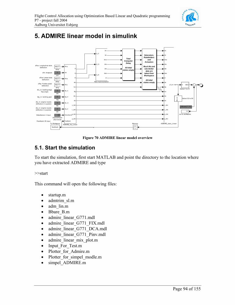
Flight Control Allocation using Optimization Based Linear and Quadratic programming P7 - project fall 2004 Aalborg Universitet Esbjerg
5. ADMIRE linear model in simulink
dVt:
dFas:
dFrp:
dFes: Longitudinal stick deflection
dVt: Airspeed
dFas: Lateral stick deflection
dFrp: Fudder pedal deflection
dle_in: leading-edge flap angle
ldg_in: landing gear
dty_in: engine nozzle-deflection in xy-plane
dtz_in: engine nozzle-deflection in xz-plane
Disturbance: 4 input
Feedback: 28 input
1
y0bare(1:31)
In1
out to workspace
0
ldg
0
dtz
0
dty
0
dle
0
dVt
step14
dFrp
step12
dFes
step12
dFas
feedback
To Workspace
U
U(E) Select 32 to 59
U U(E)
Select 1 to 31
in_P
in_Q
in_R
drc
dlc
droe
drie
dlie
dloe
dr
New implimentation
Memory
TotalComputer
Delay
All initalstates empty
Saturators,Ratelimiters
andActuators
Mach No andrate limiter
data aretaken fromWorkspace
All initalstates empty
dist
DisturbParam(Sub block)
dFes
dVt
dFas
dFrp
dle_in
ldg_in
dty _in
dtz_in
Disturbance
Feedback
P
Q
R
dle
tss
ldg
dty
dtz
u_dist
v _dist
w_dist
p_dist
ADMIRE_fcs_Linear
drc
dlc
droe
drie
dlie
dloe
dr
dle
ldg
tss
dty
dtz
u_dist
v _dist
w_dist
p_dist
y 0_lin
ADMIRE_bare_Linear
Figure 70 ADMIRE linear model overview
5.1. Start the simulation To start the simulation, first start MATLAB and point the directory to the location where you have extracted ADMIRE and type >>start This command will open the following files:
• startup.m • admtrim_sl.m • adm_lin.m • Bbare_B.m • admire_linear_G771.mdl • admire_linear_G771_FIX.mdl • admire_linear_G771_DCA.mdl • admire_linear_G771_Pinv.mdl • admire_linear_mix_plot.m • Input_For_Test.m • Plotter_for_Admire.m • Plotter_for_simpel_modle.m • simpel_ADMIRE.m
Page 94 of 155

Flight Control Allocation using Optimization Based Linear and Quadratic programming P7 - project fall 2004 Aalborg Universitet Esbjerg
5.1.1. Startup.m This file sets up the Matlab path and references the different parts in ADMIRE.
5.1.2. admtrim_sl.m The Matlab file admtrim_sl.m calls the functions in setup_ratelims.m and uncertainty.m. These .m files set up the necessary parameters used in the simulation, such as the uncertainties and the rate and position limits for the actuators.
5.1.3. adm_lin.m adm_lin.m creates the matrices for the two state space models in the linear model by calling two files, linmod_nnt.m and admire_bare_lin.mdl. These matrices describe the linearized aircraft model at the given flight condition.
5.1.4. linmod_nnt.m This is a modified model of the Matlab function linmod. Simulink provides the linmod functions to extract linear models in the form of state-space matrices A, B, C, and D. This file is called by the file adm_lin.m. State-spaces matrices describe the linear input-output relationship as:
Eq. 5-1 uxyuxx
DCBA
+=+=
where x, u, and y are state, input, and output vectors, respectively.
5.1.5. admire_bare_lin.mdl This file is called by the file adm_lin.m. This model is a quite complex simulink model which is used for configuration of the dynamic aerodynamic aircraft model.
5.1.6. Bbare_B.m This file makes a sub-matrix from the Bbare matrix in the dynamic system of the airplane. The sub-matrix (B) is used to convert the output, P, Q and Beta, from the controller and map those into the angular accelerations in pitch, roll and yaw. Information of the desired moment is the essence of control allocation in applications of flight control. The B matrix defined by this .m file is the control effectiveness matrix.
5.1.7. admire_linear_G771.mdl This file is the linear simulink model, which is the main file for simulating the aircraft dynamics with control law and control selector modules. This file is the original ADMIRE linearized model. After it appears the simulation can be run.
Page 95 of 155

Flight Control Allocation using Optimization Based Linear and Quadratic programming P7 - project fall 2004 Aalborg Universitet Esbjerg Use the pull-down menu simulation and press start to run the simulation. The time step for the simulation is set to 0.008 s. Such a short time step is required for the padé approximations of the time delays to work properly. More about this later.
5.1.8. admire_linear_G771_FIX.mdl This file is the linear simulink model, which is the main file for simulating the aircraft dynamics with control law and the Fixed-point algorithm implemented as the control allocater. After it appears the simulation can be run. Use the pull-down menu simulation and press start to run the simulation. The time step for the simulation is set to 0.008 s. Such a short time step is required for the padé approximations of the time delays to work properly.
5.1.9. admire_linear_G771_DCA.mdl This file is the linear simulink model, which is the main file for simulating the aircraft dynamics with control law and the Direct Control Allocation algorithm implemented as the control allocater. After it appears the simulation can be run. Use the pull-down menu simulation and press start to run the simulation. The time step for the simulation is set to 0.008 s. Such a short time step is required for the padé approximations of the time delays to work properly.
5.1.10. admire_linear_G771_Pinv.mdl This file is the linear simulink model, which is the main file for simulating the aircraft dynamics with control law and the Pseudoinverse algorithm implemented as the control allocater. After it appears the simulation can be run. Use the pull-down menu simulation and press start to run the simulation. The time step for the simulation is set to 0.008 s. Such a short time step is required for the padé approximations of the time delays to work properly.
5.1.11. admire_linear_mix_plot.m This file can be used to plot the simulated results of the aircraft response. After the simulation has been rune this file can be run. This file will then plot the result from the simulation. However, it should be mention that it only works with the simulation in admire_linear_G771.mdl.
5.1.12. Input_For_Test This file sets up all the input variables for the test. Within this file can the different input bee manipulated.
5.1.13. Plotter_for_Admire.m This file can be rune when all the fore simulations have been run. It will then plot the results from the simulations, in a way where it is easy to compeer the results from the different simulations.
Page 96 of 155

Flight Control Allocation using Optimization Based Linear and Quadratic programming P7 - project fall 2004 Aalborg Universitet Esbjerg
5.1.14. Plotter_for_simpel_modle.m This file can be rune when the simulations in the simple_ADMIRE.mdl file has been run. It will the plot the results from the simulation, in a way where it is easy to compeer the results from the simulation.
5.1.15. simple_ADMIRE.mdl This file is a simulation environment set up for testing the three different algorithms simultaneous. There are a number of different possibilities for setting the input. This explained in the model.
5.2. Description of admire_linear_G771_xxx.mdl First, all the inputs and outputs for this block will be explained and afterwards the sub blocks will be described in detail. The model is described by the ADMIRE team as “mainly linear” which describes the dynamics of a small generic fighter aircraft with one engine. This aircraft is a bit larger than the JAS39 and with a lower wing loading. The model is implemented as several c-mex-files in order to fit into the Simulink environment. It is based on GAM (Generic Aerodata Model) developed by Saab AB, Sweden. The simulink model admire_linear.mdl will be described in detail in the following section. First, all the input and outputs for the block will be explained, and then each sub-block will be described.
5.2.1. ADMIRE_fcs_Linear The first block, “ADMIRE_fcs_Linear”, has 10 inputs and 12 outputs, se the explanation in Table 1.
Table 1 input and output variables for the block ADMIRE_fcs_Linear Input Explanation dFes Longitudinal stick deflection dVt Airspeed dFas Lateral stick deflection dFrp Rudder pedal deflection dle_in Leading-edge flap angle ldg_in Landing gear dty_in Engine nozzle-deflection in the xy-plan dtz_in Engine nozzle-deflection in the xz-plan Disturbance 4 input u_dist, v_dist, w_dist and p_dist Feedback 27 input from feedback (State space model in the block
ADMIRE_bare_Linear) Output p Roll angular rate q Pitch angular rate
Page 97 of 155

Flight Control Allocation using Optimization Based Linear and Quadratic programming P7 - project fall 2004 Aalborg Universitet Esbjerg beta Sideslip angle dle Leading-edge flap angle tss Throttle setting ldg Landing gear dty Engine nozzle-deflection in xy-plan dtz Engine nozzle-deflection in xz-plan u_dist Turbulence in x axis v_dist Turbulence in y axis w_dist Turbulence in z axis p_dist Turbulence around roll axis ADMIRE_fcs_linear is a sub block containing a 10 to 1 multiplexer and a 1 to 12 de-multiplexer. Furthermore it includes a state-space block which has the following four matrices: Afcs (dim 4x4), Bfcs (dim 4x40), Cfcs (dim 12x4) and Dfcs (dim 12x40). This state space model acts as the controller for the aircraft. Its input and output is described above in Table 1. p,q and beta are the first three outputs and these connect to the input of the “control selector block”. The next two output, dle and tss, is connected to the “Saturators, Rate limiters and Actuators” block. The last seven outputs, ldg, dty, dtz, u_dist, v_dist, w_dist, and p_dist are connected directly to the last block, “ADMIRE_bare_Linear”.
5.2.2. Control Selector The control selector is a sub-block contains the block, “FCS_cs” which has 5 inputs and 7 outputs. The description of the inputs and outputs can be seen in Table 2.
Table 2 input and output variables for the control selector block Input Explanation p Roll angular rate q Pitch angular rate beta Sideslip angle Alt+dalt_err Altitude + difference in the altitude error Mach+dMach_err Speed (mach) + difference in the speed error Output drc Right canard angle deflection dlc Left canard angle deflection droe Right outer elevon angle deflection drie Right inner elevon angle deflection dlie Left inner elevon angle deflection dloe Left outer elevon angle deflection dr Rudder angle deflection
Page 98 of 155

Flight Control Allocation using Optimization Based Linear and Quadratic programming P7 - project fall 2004 Aalborg Universitet Esbjerg
5.2.3. FCS_cs The block FCS_cs is a sub-block located in Control Selector and contains a sub-block named FCS_cs_table and a number of summations elements, a multiplexer and four de-multiplexers. The multiplexer joins 21 outputs from the FCS_cs_table block into a single vector. After combining the inputs, the vector of 21 elements is split up in to three vectors: One containing the first 7 elements, the second containing the next 7 elements and last the third containing the last 7 elements. After splitting the vectors into smaller vectors, these are multiplied by p, q, and beta. The first vector is multiplied by p, the second by q and the third by beta. Each of the three vectors are then de-multiplexed into 21 signals. The signals are then summed together in the following way: Signal one from vector one is summed with signal one from the second and third vector, the second signal from each array is summed together the same way as the remaining five signals. These calculations produce the 7 signals which are the outputs from this block. These output signals represent the control signals sent to the actuators. See Figure 71 for reference.
p
q
beta
7
FCS_cs_dr
6
FCS_cs_dloe
5
FCS_cs_dlie
4
FCS_cs_drie
3
FCS_cs_droe
2
FCS_cs_dlc
1
FCS_cs_drc
Mux
FCS_cs_table
FCS_cs_table
em
Demux3
em
em
Demux1
em
Demux
5
FCS_cs_beta
4
FCS_cs_q
3
FCS_cs_p
2
FCS_cs_Mach
1
FCS_cs_Altitude
Figure 71 An overview of the sub-block FCS_cs
FCS_cs_table contains the block ‘fcsselector’ and a demultiplexer. The demultiplexer splits the signals from the S-function ‘fcsselector’ into 21 single signals (see Figure 71). fcsselector This block contains an S-Function called ‘fcsselector’. This S-function is made from a c-file, which decides what weighting the 21 outputs should have according to the altitude and Mach number. The S-Function delivers its output vector to a de-multiplexer which splits the vector up into 21 single signals. These 21 outputs then represent how to weigh p, q and beta from the controller and map these onto the control surfaces of the aircraft.
Page 99 of 155

Flight Control Allocation using Optimization Based Linear and Quadratic programming P7 - project fall 2004 Aalborg Universitet Esbjerg This is the simple control allocation block of ADMIRE. The calculations in this block determine the outputs for the seven control surfaces. The input and output can be seen in Table 3.
Table 3 Input and output from the block FCS_cs_table Input Explanation (1) FCS_cs_table_Altitude Altitude (2) FCS_cs_table_Mach Mach number Output (1) FCS_cs_table_p_drc (2) FCS_cs_table_p_dlc (3) FCS_cs_table_p_droe (4) FCS_cs_table_p_drie (5) FCS_cs_table_p_dlie (6) FCS_cs_table_p_dloe (7) FCS_cs_table_p_dr (8) FCS_cs_table_q_drc (9) FCS_cs_table_q_dlc (10) FCS_cs_table_q_droe (11) FCS_cs_table_q_drie (12) FCS_cs_table_q_dlie (13) FCS_cs_table_q_dloe (14) FCS_cs_table_q_dr (15) FCS_cs_table_beta_drc (16) FCS_cs_table_beta_dlc (17) FCS_cs_table_beta_droe (18) FCS_cs_table_beta_drie (19) FCS_cs_table_beta_dlie (20) FCS_cs_table_beta_dloe (21) FCS_cs_table_beta_dr
5.2.4. New implementation The block ‘New implementation’ is a new block. This block is the place for our implementation of a control allocator. The input to this block comes from the Controller block, and it sends its output to the block total computer delay. In our implementation, a mapping must be made from the desired moments commanded by the controller, into control surface deflections of the aircraft. The dynamic response of the aircraft after using our new control allocator should be very close to the response of the aircraft when using ADMIRE’s own built-in allocator. Depending on the choice of algorithm for performing control allocation the aircraft response will differ slightly under some conditions. As mentioned in former chapters, the direct allocation implemented using linear programming provides directionality by sacrificing moment generation, while the control minimization is implemented using the cascaded generalized inverse sacrifices directionality while attempting to preserve moment generation.
Page 100 of 155

Flight Control Allocation using Optimization Based Linear and Quadratic programming P7 - project fall 2004 Aalborg Universitet Esbjerg
5.2.5. Total computer delay The block, ‘Total computer delay’ is a sub-system containing a delay element for each of the seven input signals. The delay is produced by a second order filter. Each of the seven inputs is routed through this block with a delay of 20 milliseconds. The seven inputs are taken from the FCS_cs block. The output is sent to the ‘saturators, rate limiters and actuators’ block.
5.2.6. Saturators, rate limiters and actuators The block ‘saturators, rate limiters and actuators’ provide the system with information on the actuator’s limitations in both position and angular rate. These limitations are functions of the Mach number and the altitude. The work done in this block is to test if the actuators are saturated in either rate or position. The position limitation checking is performed by the S-Function ‘act_pos_lim’, which simply compares the actual value with the saturation value. If any input is exceeding saturation limits, this function clips the output to the actuator to the saturated values for the corresponding actuator, thereby simulating real world actuators which have their saturation limits. The block has ten inputs and nine outputs see Table 4.
Table 4: Input and output from the block ’saturators, rate limiters and actuators’ Input Explanation FCS_ae_rl_drc Right canard angle FCS_ae_rl_dlc Left canard angle FCS_ae_rl_droe Right inboard elevon angle FCS_ae_rl_drie Right outboard elevon angle FCS_ae_rl_dlie Left outboard elevon angle FCS_ae_rl_dloe Left inboard elevon angle FCS_ae_rl_dr Rudder angle FCS_ae_rl_dle Leading-edge flap angle FCS_ae_rl_tss Throttle setting Mach Mach number Output FCS_ae_rl_drc_out Right canard angle FCS_ae_rl_dlc_out Left canard angle FCS_ae_rl_droe_out Right inboard elevon angle FCS_ae_rl_drie_out Right outboard elevon angle FCS_ae_rl_dlie_out Left outboard elevon angle FCS_ae_rl_dloe_out Left inboard elevon angle FCS_ae_rl_dr_out Rudder angle FCS_ae_rl_dle_out Leading-edge flap angle FCS_ae_rl_tss_out Throttle setting The subsystem contains a rate limitation block, see Table 5. The rate limitations of the actuators are determined by a first order system. Each first order system is dependant of
Page 101 of 155

Flight Control Allocation using Optimization Based Linear and Quadratic programming P7 - project fall 2004 Aalborg Universitet Esbjerg an initial value, except for the first order system related to the engine. The engine rate limiter is determined with a specific first order system.
Table 5: Sub-system name System name File name FCS_ae_rl_rc Admire_linear/FCS_ae_rl/FCS_ae_rl_rc FCS_ae_rl_lc Admire_linear/FCS_ae_rl/FCS_ae_rl_lc FCS_ae_rl_roe Admire_linear/FCS_ae_rl/FCS_ae_rl_roe FCS_ae_rl_rie Admire_linear/FCS_ae_rl/FCS_ae_rl_rie FCS_ae_rl_lie Admire_linear/FCS_ae_rl/FCS_ae_rl_lie FCS_ae_rl_loe Admire_linear/FCS_ae_rl/FCS_ae_rl_loe FCS_ae_rl_r Admire_linear/FCS_ae_rl/FCS_ae_rl_r FCS_ae_rl_le Admire_linear/FCS_ae_rl/FCS_ae_rl_le
5.2.7. ADMIRE_bare_Linear The block ‘ADMIRE_bare_Linear’ is a subsystem containing a state-space model. This model has 16 inputs and 59 outputs. The matrices in this block is: Abare (dim 28 x 28), Bbare (dim 28 x 16), Cbare (dim 59 x 28) and Dbare,(dim 59 x 16). These four matrices describe the state-space model which represents the linearized aircraft dynamics under certain flight conditions described by the Mach number and the altitude of the aircraft. The 16 inputs consist of the following variables, as can be seen in Table 5.
Table 6: Input for ADMIRE_bare_Linear Input Explanation drc Right canard angle dlc Left canard angle droe Right outboard elevon angle drie Right inboard elevon angle dlie Left inboard elevon angle dloe Left outboard elevon angle dr Rudder angle dle Leading-edge flap angle ldg Landing gear tss Throttle setting dty Engine nozzle-deflection in the xy-plane dtz Engine nozzle-deflection in the xz-plane u_dist Turbulence in x axis v_dist Turbulence in y axis w_dist Turbulence in z axis p_dist Turbulence around roll axis Since the output variables from the block containing both output and state variables, it has to be sorted. This is done by selecting the first 31 variables for output and another block for retrieving the last 27 state variables. The first 31 variables are summed together with the first 31 variables in the imported array, y0bare, and it is then sent to the output port 1 which is the output representing the aircraft current state.
Page 102 of 155

Flight Control Allocation using Optimization Based Linear and Quadratic programming P7 - project fall 2004 Aalborg Universitet Esbjerg These 31 variables can be found in Table 7.
Table 7 Output for ADMIRE_bare_Linear Output Explanation unit (1) Vt Airspeed m/s (2) alpha Angle of attack rad (3) beta Angle of sideslip rad (4) pb Roll angular rate rad/s (5) qp Pitch angular rate rad/s (6) rb Yaw angular rate rad/s (7) psi Euler angles (azimuth) rad (8) theta Euler angles (elevation) rad (9) phi Euler angles (bank) rad (10) x x position in Fv m (11) y y position in Fv m (12) z z position in Fv m (13) ub Velocity in x-axis m/s (14) vb Velocity in y-axis m/s (15) wb Velocity in z-axis m/s (16) uv Velocity in earth parallel x-axis m/s (17) vv Velocity in earth parallel y-axis m/s (18) wv Velocity in earth parallel z-axis m/s (19) nz Normal acceleration of c.g. “g” (20) ny Side acceleration of c.g. “g” (21) mach Mach number - (22) gamma Climb angle rad (23) cd Drag coefficient - (24) cl Lift coefficient - (25) cc Side force coefficient - (26) crm Roll coefficient - (27) cpm Pitch coefficient - (28) cym Yaw coefficient - (29) not defined - (30) not defined - (31) not defined - The 27 state variables are sent to a memory block and then used for feedback to the block, ’ADMIRE_fcs_linear’. The signals have the same denomination as the first 27 elements in the 31 output variables.
Page 103 of 155

Flight Control Allocation using Optimization Based Linear and Quadratic programming P7 - project fall 2004 Aalborg Universitet Esbjerg
5.2.8. disturbParam The block ‘disturbParam’ is a subsystem containing four inputs giving on four channel output. The four inputs, see Table 8, are multiplexed to become a vector and then output as ‘dist’.
Table 8: Input and output to the block DisturbParam. Indput Explanation u_dist Turbulence in x axis v_dist Turbulence in y axis w_dist Turbulence in z axis p_dist Turbulence around roll axis Output dist Input to ADMIRE_fcs_Linear
6. Implementation in ADMIRE The control selector box in ADMIRE works as most existing ganging methods. However, the control selector in ADMIRE also takes into account the Mach number and the altitude. The controller of ADMIRE has 3 control outputs. P, Q and R. In conventional aircraft terminology, these variables determine the roll-rate, yaw-rate respectively. In the control selector box these 3 input variables are used to produce the control signals for the 7 actuators. In this project we require the 3 commanded moments in the rolling, pitching and yawing direction. To obtain the control vector (v) it’s necessary to “roll back” the 7 actuator control signals from the control selector box. This is done by picking out the columns and rows in the B-matrix of the state-space model describing the linearized dynamics of the actuators in the ADMIRE model. Ola Härkegård confirmed on e-mail the 14th of October 2004 that we should define the control effectiveness matrix (B) as: Eq. 6-1 ( )7:1,6:4BbareB = Since p, q and r are states 4, 5, 6 and since there’s seven control surfaces. This operation defines a new matrix B, which is our control effectiveness matrix for the aircraft at the specified flight condition. Multiplying the output of the control selector by B we obtain the angular accelerations in roll, pitch and yaw. Using this vector as input to our control allocation algorithm, we need to make some approximations of the aircraft model.
• Ignoring actuator dynamics • Viewing control surfaces as moment generators • Consider only position constraints
These approximations make it possible to consider the control allocation problem much simpler. By ignoring actuator dynamics, we assume that the actuators are capable of moving indefinitely fast and without offset problems. The actuator rate limitations will only pose a problem when the input to the control allocator changes instantly with a large
Page 104 of 155

Flight Control Allocation using Optimization Based Linear and Quadratic programming P7 - project fall 2004 Aalborg Universitet Esbjerg magnitude. Since the input to the control allocator is described by the output of the controller, the input should not change instantly. Further, by viewing the control surfaces as moment generators, we can obtain a direct coherency between an exact actuator position and a generated aerodynamic moment. While the actuators both have position and rate limits, the easiest part to consider are the position constraints. It’s not impossible to also include rate constraints, but in this project we will focus only on position constraints. The methods used in this project are implemented only to consider position limitations. Using other methods and algorithms it’s possible to consider actuator rate constraints as well.
6.1. Flight conditions During the testing of an aircraft response, it’s important to settle on a given flight condition, since flight as a general case is highly non-linear, one must decide which flight conditions are feasible for a test scenario in order to keep the test size down. At each flight condition, the dynamics of the aircraft are slightly changed, if each flight condition should be tested, the test itself would be a project on its own. The two most significant variables to be determined beforehand are the Mach number and the altitude of the flight. In our testing scenario, the group settled for a Mach number of 0.5 and an altitude of 1000m.
Page 105 of 155

Flight Control Allocation using Optimization Based Linear and Quadratic programming P7 - project fall 2004 Aalborg Universitet Esbjerg
7. ADMIRE simulation The real simulation of the algorithms will be conducted in the aircraft benchmark ADMIRE. As described in previous chapters, the model used in ADMIRE is the linear model, which is trimmed at a certain flight condition. The ADMIRE test section is divided into 4 tests. The first two tests consist of step inputs. The last two tests consist of 2 ramp inputs. Ola Härkegård confirmed on e-mail 2nd of november that the inputs Fes, Fas, and Frp are all limited to a range of possible inputs. These ranges are: Table 6 Input limitations
Input Positive limit Negative limit Fes 80 -40 Fas 80 -80 Frp 200 -200
7.1. Test 1 The first test gives a step input to the ADMIRE model, using the following values:
Input Step magnitude Fes 50 Fas 50 Frp 120
The step is given after 1 second simulation.
0 1 2 3 4 5 6 7 8 9 10-2
0
2
4
6
8
10
moment (N)
Desired moment P
PinvFIXDCAADMIRE
0 1 2 3 4 5 6 7 8 9 10-2
0
2
4
6
8
10
time(sec)
moment (N)
Achieved moment P
PinvFIXDCAADMIRE
Figure 72: Test1 - commanded and achieved moment for p
Page 106 of 155
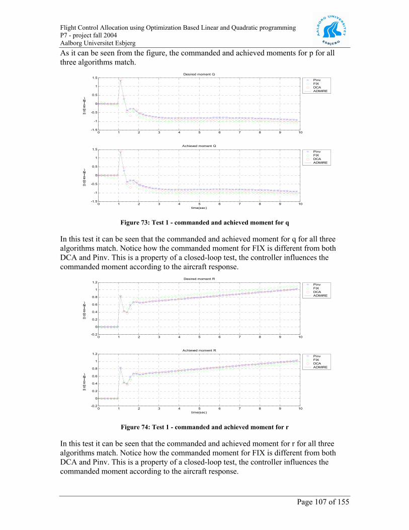
Flight Control Allocation using Optimization Based Linear and Quadratic programming P7 - project fall 2004 Aalborg Universitet Esbjerg As it can be seen from the figure, the commanded and achieved moments for p for all three algorithms match.
0 1 2 3 4 5 6 7 8 9 10-1.5
-1
-0.5
0
0.5
1
1.5
moment (N)
Desired moment Q
PinvFIXDCAADMIRE
0 1 2 3 4 5 6 7 8 9 10-1.5
-1
-0.5
0
0.5
1
1.5
time(sec)
moment (N)
Achieved moment Q
PinvFIXDCAADMIRE
Figure 73: Test 1 - commanded and achieved moment for q
In this test it can be seen that the commanded and achieved moment for q for all three algorithms match. Notice how the commanded moment for FIX is different from both DCA and Pinv. This is a property of a closed-loop test, the controller influences the commanded moment according to the aircraft response.
0 1 2 3 4 5 6 7 8 9 10-0.2
0
0.2
0.4
0.6
0.8
1
1.2
moment (N)
Desired moment R
PinvFIXDCAADMIRE
0 1 2 3 4 5 6 7 8 9 10-0.2
0
0.2
0.4
0.6
0.8
1
1.2
time(sec)
moment (N)
Achieved moment R
PinvFIXDCAADMIRE
Figure 74: Test 1 - commanded and achieved moment for r
In this test it can be seen that the commanded and achieved moment for r for all three algorithms match. Notice how the commanded moment for FIX is different from both DCA and Pinv. This is a property of a closed-loop test, the controller influences the commanded moment according to the aircraft response.
Page 107 of 155

0 1 2 3 4 5 6 7 8 9 10-15
-10
-5
0
5
10
deflection (deg)
Actuator output signal drc
PinvFIXDCAADMIRE
0 1 2 3 4 5 6 7 8 9 10-15
-10
-5
0
5
10
time(sec)
deflection (deg)
Actuator output signal dlc
PinvFIXDCAADMIRE
Flight Control Allocation using Optimization Based Linear and Quadratic programming P7 - project fall 2004 Aalborg Universitet Esbjerg
Page 108 of 155
Figure 75: Test 1 - Right canard and left canard deflection
The upper graph shows the right canard deflection while the bottom graph shows the left canard deflection. The FIX algorithm commands a larger deflection of both canards, while DCA comes in at second place with a little less deflection. Pinv commands the least deflection of the three. None of the algorithms saturate either of the canards.
0 1 2 3 4 5 6 7 8 9 10-14
-12
-10
-8
-6
-4
-2
0
deflection (deg)
Actuator output signal droe
PinvFIXDCAADMIRE
0 1 2 3 4 5 6 7 8 9 10-20
-15
-10
-5
0
time(sec)
deflection (deg)
Actuator output signal drie
PinvFIXDCAADMIRE
Figure 76: Test 1 - Right outer and inner elevon deflection
The upper graph shows the right outer elevon deflection, while the lower graph shows the right inner elevon deflection. All three algorithms show a similar curve shape, while the FIX algorithm commands the largest deflection, DCA comes second and Pinv commands the least deflection. None of the algorithms saturate either right elevon.

0 1 2 3 4 5 6 7 8 9 10-10
-5
0
5
10
time(sec)
deflection (deg)
Actuator output signal dlie
PinvFIXDCAADMIRE
0 1 2 3 4 5 6 7 8 9 10-4
-2
0
2
4
6
8
10
deflection (deg)
Actuator outout signal dloe
PinvFIXDCAADMIRE
Flight Control Allocation using Optimization Based Linear and Quadratic programming P7 - project fall 2004 Aalborg Universitet Esbjerg
Page 109 of 155
Figure 77: Test 1 - Left outer and inner elevon deflection
The upper graph shows the left outer elevon deflection, while the lower graph shows the left inner elevon deflection. All three algorithms show a similar curve shape, but in this case the FIX algorithm commands the smallest deflection. DCA comes second while Pinv comes in last with the largest deflection. None of the algorithms saturate either of the left elevons.
0 1 2 3 4 5 6 7 8 9 10-6
-4
-2
0
2
time(sec)
deflection (deg)
Actuator output signal dr
PinvFIXDCAADMIRE
Figure 78: Test 1 - Rudder deflection
The graph shows the rudder deflection. All three algorithms show a similar curve shape, while DCA commands the largest deflection, Pinv commands less deflection and the FIX algorithm commands the smallest deflection of the rudder. None of the algorithms saturate the rudder.

0 1 2 3 4 5 6 7 8 9 10-200
-150
-100
-50
0
50ADMIRE
x [m]
PinvFIXDCAADMIRE
0 1 2 3 4 5 6 7 8 9 10-1000
0
1000
2000
3000
y [m]
PinvFIXDCAADMIRE
0 1 2 3 4 5 6 7 8 9 10-2500
-2000
-1500
-1000
-500
z [m]
time (sec)
PinvFIXDCAADMIRE
Flight Control Allocation using Optimization Based Linear and Quadratic programming P7 - project fall 2004 Aalborg Universitet Esbjerg
Page 110 of 155
Figure 79: Test 1 - Aircraft X-Y-Z movement
This figure shows the aircraft movement in the X-Y-Z directions. Notice how the representation of the aircraft movement is according to its trimmed altitude and Mach number. The position of the aircraft is given without including the integral of its trimmed velocity. Especially this can be seen in the x-plot, where the position of the aircraft should increase with time according to the speed of 0.5 Mach. Instead we can see a decrease in position. This merely means that the aircraft velocity is decreasing through the simulation. By inspection, the middle graph and the lower graph show all three algorithms behave identical. The upper graph, however, shows some difference between the three. Pinv tracks the ADMIRE trajectory without error, while DCA comes very close. The FIX algorithm is a little more off than both DCA and Pinv.
7.2. Test 2 The second test gives a step input to the ADMIRE model, using the following values:
Input Step magnitude Fes -30 Fas -50 Frp -120

Flight Control Allocation using Optimization Based Linear and Quadratic programming P7 - project fall 2004 Aalborg Universitet Esbjerg The step is given after 1 second simulation.
0 1 2 3 4 5 6 7 8 9 10-10
-8
-6
-4
-2
0
2
moment (N)
Desired moment P
PinvFIXDCAADMIRE
0 1 2 3 4 5 6 7 8 9 10-10
-8
-6
-4
-2
0
2
time(sec)
moment (N)
Achieved moment P
PinvFIXDCAADMIRE
Figure 80: Test 2 - commanded and achieved moment for p
As it can be seen from the figure, the commanded and achieved moments for p for all three algorithms match.
0 1 2 3 4 5 6 7 8 9 10-1
-0.5
0
0.5
1
moment (N)
Desired moment Q
PinvFIXDCAADMIRE
0 1 2 3 4 5 6 7 8 9 10-1
-0.5
0
0.5
1
time(sec)
moment (N)
Achieved moment Q
PinvFIXDCAADMIRE
Figure 81: Test 2 - commanded and achieved moment for q
In this test it can be seen that the commanded and achieved moment for q for all three algorithms match. Notice how the commanded moment for FIX is different from both DCA and Pinv. This is a property of a closed-loop test, the controller influences the commanded moment according to the aircraft response.
Page 111 of 155

0 1 2 3 4 5 6 7 8 9 10-1.2
-1
-0.8
-0.6
-0.4
-0.2
0
0.2
moment (N)
Desired moment R
PinvFIXDCAADMIRE
0 1 2 3 4 5 6 7 8 9 10-1.2
-1
-0.8
-0.6
-0.4
-0.2
0
0.2
time(sec)
moment (N)
Achieved moment R
PinvFIXDCAADMIRE
Flight Control Allocation using Optimization Based Linear and Quadratic programming P7 - project fall 2004 Aalborg Universitet Esbjerg
Page 112 of 155
Figure 82: Test 2 - commanded and achieved moment for r
In this test it can be seen that the commanded and achieved moment for r for all three algorithms match. Notice how the commanded moment for FIX is different from both DCA and Pinv. This is a property of a closed-loop test, the controller influences the commanded moment according to the aircraft response.
0 1 2 3 4 5 6 7 8 9 10-15
-10
-5
0
5
deflection (deg)
Actuator output signal drc
PinvFIXDCAADMIRE
0 1 2 3 4 5 6 7 8 9 10-15
-10
-5
0
5
time(sec)
deflection (deg)
Actuator output signal dlc
PinvFIXDCAADMIRE
Figure 83: Test 2 - Right canard and left canard deflection
The upper graph shows the right canard deflection while the bottom graph shows the left canard deflection. The FIX algorithm commands a larger deflection of both canards, while DCA comes in at second place with a little less deflection. Pinv commands the least deflection of the three. None of the algorithms saturate either of the canards.

0 1 2 3 4 5 6 7 8 9 10-4
-2
0
2
4
6
8
10
deflection (deg)
Actuator output signal droe
PinvFIXDCAADMIRE
0 1 2 3 4 5 6 7 8 9 10-10
-5
0
5
10
time(sec)
deflection (deg)
Actuator output signal drie
PinvFIXDCAADMIRE
Flight Control Allocation using Optimization Based Linear and Quadratic programming P7 - project fall 2004 Aalborg Universitet Esbjerg
Page 113 of 155
Figure 84: Test 2 - Right outer and inner elevon deflection
The upper graph shows the right outer elevon deflection, while the lower graph shows the right inner elevon deflection. All three algorithms show a similar curve shape, while the FIX algorithm commands the smallest deflection, Pinv comes second and DCA commands the largest deflection. None of the algorithms saturate either right elevon.
0 1 2 3 4 5 6 7 8 9 10-14
-12
-10
-8
-6
-4
-2
0
time(sec)
deflection (deg)
Actuator output signal dlie
PinvFIXDCAADMIRE
0 1 2 3 4 5 6 7 8 9 10-10
-8
-6
-4
-2
0
deflection (deg)
Actuator outout signal dloe
PinvFIXDCAADMIRE
Figure 85: Test 2 - Left outer and inner elevon deflection
The upper graph shows the left outer elevon deflection, while the lower graph shows the left inner elevon deflection. All three algorithms show a similar curve shape. In this case the FIX algorithm commands the largest deflection. DCA comes second while Pinv comes in last with the smallest deflection. None of the algorithms saturate either of the left elevons.

Flight Control Allocation using Optimization Based Linear and Quadratic programming P7 - project fall 2004 Aalborg Universitet Esbjerg
0 1 2 3 4 5 6 7 8 9 10-2
-1
0
1
2
3
4
5
time(sec)
deflection (deg)
Actuator output signal dr
PinvFIXDCAADMIRE
Figure 86 Test 2 - Rudder deflection
The graph shows the rudder deflection. All three algorithms show a similar curve shape, while DCA commands the largest deflection, Pinv commands less deflection and the FIX algorithm commands the smallest deflection of the rudder. None of the algorithms saturate the rudder.
0 1 2 3 4 5 6 7 8 9 10-100
0
100
200
300ADMIRE
x [m]
PinvFIXDCAADMIRE
0 1 2 3 4 5 6 7 8 9 10-3000
-2000
-1000
0
1000
y [m]
PinvFIXDCAADMIRE
0 1 2 3 4 5 6 7 8 9 10-1500
-1000
-500
0
z [m]
time (sec)
PinvFIXDCAADMIRE
Figure 87: Test 2 - Aircraft X-Y-Z movement
As mentioned in test 1, the graphs represent the aircraft movement in X-Y-Z directions without the integral of the trimmed velocity. By inspection, the middle graph and the lower graph show all three algorithms behave identical. The upper graph, however, shows some difference between the three. Pinv
Page 114 of 155

Flight Control Allocation using Optimization Based Linear and Quadratic programming P7 - project fall 2004 Aalborg Universitet Esbjerg tracks the ADMIRE trajectory without error, while DCA comes very close. The FIX algorithm is a little more off than both DCA and Pinv.
7.3. Test 3 The third test gives a ramp input to the ADMIRE model, using the following values:
Input Ramp slope Fes 40/sec Fas 40/sec Frp 100/sec
The ramp is given after 1 second simulation.
0 1 2 3 4 5 6 7 8 9 10-10
0
10
20
30
40
50
60
moment (N)
Desired moment P
PinvFIXDCAADMIRE
0 1 2 3 4 5 6 7 8 9 10-10
0
10
20
30
40
50
60
time(sec)
moment (N)
Achieved moment P
PinvFIXDCAADMIRE
Figure 88: Test 3 - commanded and achieved moment for p
As it can be seen from the figure, the commanded and achieved moments for p for all three algorithms aren’t equal. Pinv produce some fluctuations in both commanded and achieved moment while both DCA and FIX produce steady moments.
Page 115 of 155

Flight Control Allocation using Optimization Based Linear and Quadratic programming P7 - project fall 2004 Aalborg Universitet Esbjerg
0 1 2 3 4 5 6 7 8 9 10-20
-15
-10
-5
0
5
moment (N)
Desired moment Q
PinvFIXDCAADMIRE
0 1 2 3 4 5 6 7 8 9 10-20
-15
-10
-5
0
5
time(sec)
moment (N)
Achieved moment Q
PinvFIXDCAADMIRE
Figure 89: Test 3 - commanded and achieved moment for q
As it can be seen from the figure, the commanded and achieved moments for q for all three algorithms aren’t equal, although the achieved moment comes closer to the commanded moment than for p. Pinv produce some fluctuations in both commanded and achieved moment while both DCA and FIX produce steady moments.
0 1 2 3 4 5 6 7 8 9 10-5
0
5
10
15
moment (N)
Desired moment R
PinvFIXDCAADMIRE
0 1 2 3 4 5 6 7 8 9 10-2
0
2
4
6
8
time(sec)
moment (N)
Achieved moment R
PinvFIXDCAADMIRE
Figure 90: Test 3 - commanded and achieved moment for r
As it can be seen from the figure, the commanded and achieved moments for p for all three algorithms aren’t equal. Pinv produce some fluctuations in both commanded and achieved moment while DCA produce steady moments. The FIX algorithm stops producing moment in the end of the simulation and backs off.
Page 116 of 155

0 1 2 3 4 5 6 7 8 9 10-60
-40
-20
0
20
40
deflection (deg)
Actuator output signal drc
PinvFIXDCAADMIRE
0 1 2 3 4 5 6 7 8 9 10-60
-40
-20
0
20
40
time(sec)
deflection (deg)
Actuator output signal dlc
PinvFIXDCAADMIRE
Flight Control Allocation using Optimization Based Linear and Quadratic programming P7 - project fall 2004 Aalborg Universitet Esbjerg
Page 117 of 155
Figure 91: Test 3 – Right canard and left canard deflection
The upper graph shows the right canard deflection while the bottom graph shows the left canard deflection. Pinv commands the least deflection of the three, until at timepoint 6.5 sec. where Pinv commands erratic deflections for both canards. DCA commands the largest deflections of the left canard over time. FIX commands the largest deflection of the right canard. DCA saturates the left canard in the negative deflection, and Pinv saturates both canards in its erratic period. The FIX algorithm doesn’t saturate either canard.
0 1 2 3 4 5 6 7 8 9 10-30
-20
-10
0
10
20
30
deflection (deg)
Actuator output signal droe
PinvFIXDCAADMIRE
0 1 2 3 4 5 6 7 8 9 10-30
-20
-10
0
10
20
30
time(sec)
deflection (deg)
Actuator output signal drie
PinvFIXDCAADMIRE
Figure 92: Test 3 - Right outer and inner elevon deflection
The upper graph shows the right outer elevon deflection while the lower graph shows the right inner elevon deflection. All 3 algorithms follow the same curve shape until time point 7 sec. where Pinv commands erratic deflections. Both FIX and DCA follows the

Flight Control Allocation using Optimization Based Linear and Quadratic programming P7 - project fall 2004 Aalborg Universitet Esbjerg same curve shape through the entire simulation. Pinv commands the least deflection, until time point 7 sec. where it shows erratic behavior and saturates both elevons in the upper and lower position in turn. All algorithms saturate both elevons.
0 1 2 3 4 5 6 7 8 9 10-20
0
20
40
60
80
100
120
time(sec)
deflection (deg)
Actuator output signal dlie
PinvFIXDCAADMIRE
0 1 2 3 4 5 6 7 8 9 10-20
0
20
40
60
80
100
deflection (deg)
Actuator outout signal dloe
PinvFIXDCAADMIRE
Figure 93: Test 3 - Left outer and inner elevon deflection
In the upper graph the left outer elevon deflection is shown, while the lower graph shows the left inner elevon deflection. All 3 algorithms command the same actuator deflection, within a very small margin. All 3 algorithms saturate both elevons in the positive position.
0 1 2 3 4 5 6 7 8 9 10-30
-20
-10
0
10
20
30
time(sec)
deflection (deg)
Actuator output signal dr
PinvFIXDCAADMIRE
Figure 94: Test 3 - Rudder deflection
The graph shows the rudder deflection. All three algorithms show a similar curve shape up until time point 6.5 sec. where Pinv commands erratic deflections. While DCA commands the largest deflection before this time point, Pinv commands the largest deflection after the time point. Over time the FIX algorithm commands the smallest deflection of the rudder. Only the Pinv algorithm saturates the rudder.
Page 118 of 155
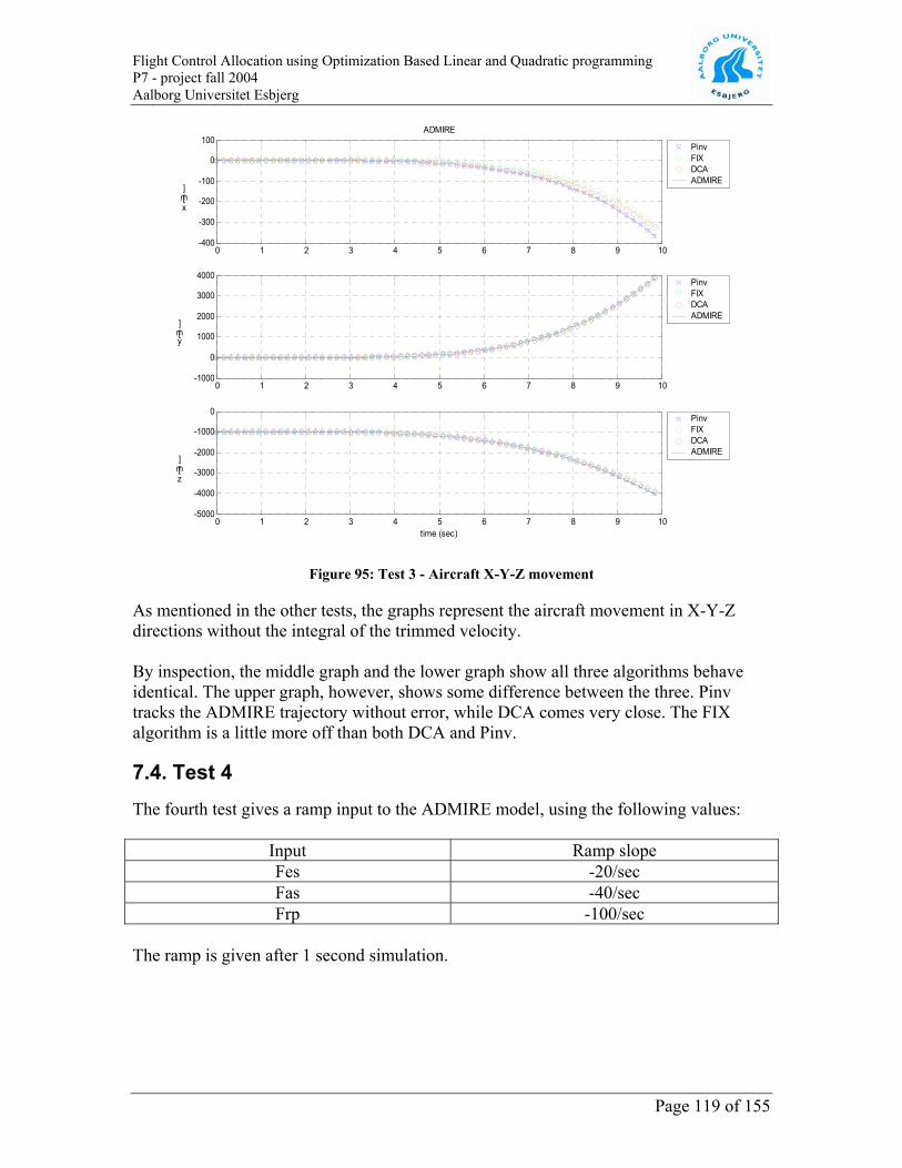
0 1 2 3 4 5 6 7 8 9 10-400
-300
-200
-100
0
100ADMIRE
x [m]
PinvFIXDCAADMIRE
0 1 2 3 4 5 6 7 8 9 10-1000
0
1000
2000
3000
4000
y [m]
PinvFIXDCAADMIRE
0 1 2 3 4 5 6 7 8 9 10-5000
-4000
-3000
-2000
-1000
0
z [m]
time (sec)
PinvFIXDCAADMIRE
Flight Control Allocation using Optimization Based Linear and Quadratic programming P7 - project fall 2004 Aalborg Universitet Esbjerg
Page 119 of 155
Figure 95: Test 3 - Aircraft X-Y-Z movement
As mentioned in the other tests, the graphs represent the aircraft movement in X-Y-Z directions without the integral of the trimmed velocity. By inspection, the middle graph and the lower graph show all three algorithms behave identical. The upper graph, however, shows some difference between the three. Pinv tracks the ADMIRE trajectory without error, while DCA comes very close. The FIX algorithm is a little more off than both DCA and Pinv.
7.4. Test 4 The fourth test gives a ramp input to the ADMIRE model, using the following values:
Input Ramp slope Fes -20/sec Fas -40/sec Frp -100/sec
The ramp is given after 1 second simulation.

0 1 2 3 4 5 6 7 8 9 10-60
-50
-40
-30
-20
-10
0
10
moment (N)
Desired moment P
PinvFIXDCAADMIRE
0 1 2 3 4 5 6 7 8 9 10-60
-50
-40
-30
-20
-10
0
10
time(sec)
moment (N)
Achieved moment P
PinvFIXDCAADMIRE
Flight Control Allocation using Optimization Based Linear and Quadratic programming P7 - project fall 2004 Aalborg Universitet Esbjerg
Page 120 of 155
Figure 96: Test 4 - commanded and achieved moment for p
As it can be seen from the figure, the commanded and achieved moments for p for all three algorithms aren’t equal. Pinv produce some fluctuations in both commanded and achieved moment while both DCA and FIX produce steady moments.
0 1 2 3 4 5 6 7 8 9 10-10
0
10
20
30
moment (N)
Desired moment Q
PinvFIXDCAADMIRE
0 1 2 3 4 5 6 7 8 9 10-5
0
5
10
15
time(sec)
moment (N)
Achieved moment Q
PinvFIXDCAADMIRE
Figure 97: Test 4 - commanded and achieved moment for q
As it can be seen from the figure, the commanded and achieved moments for q for all three algorithms aren’t equal. Pinv produce some fluctuations in both commanded and achieved moment while both DCA and FIX produce steady moments. None of the algorithms can fully track the commanded moment.
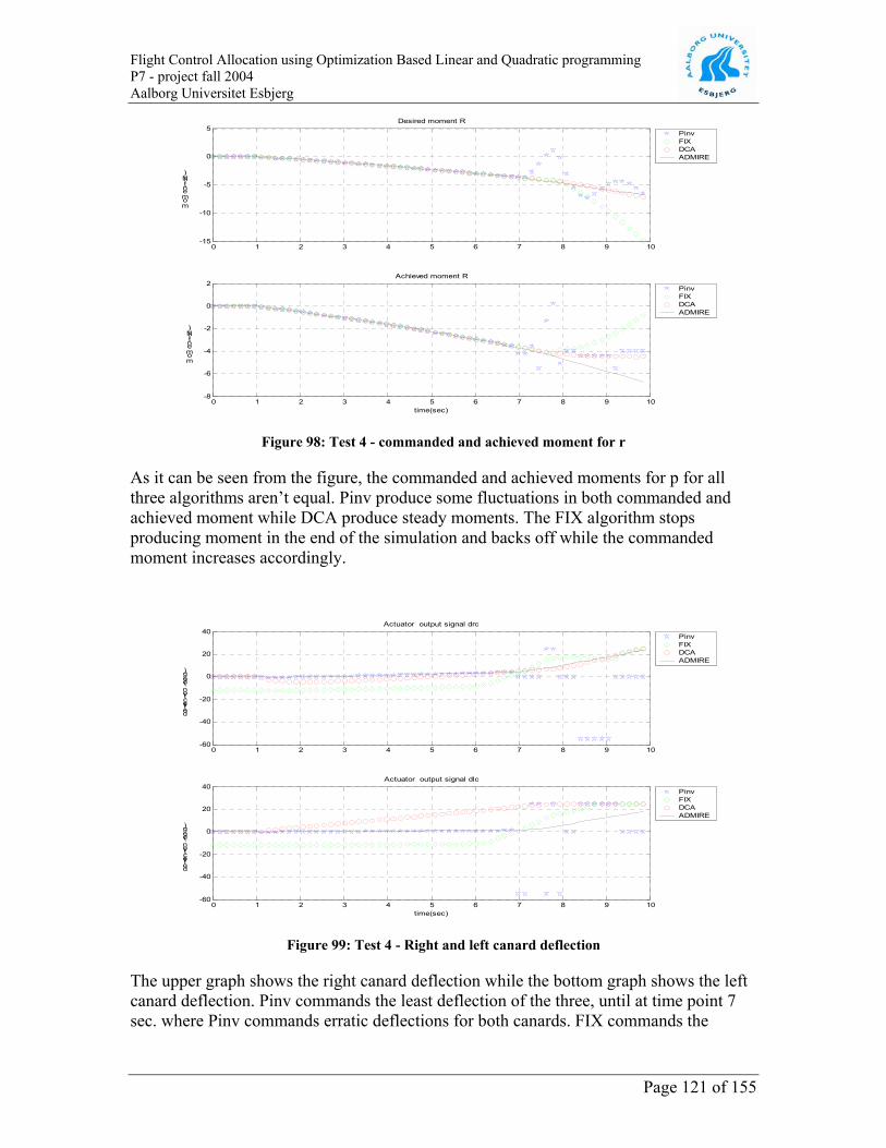
0 1 2 3 4 5 6 7 8 9 10-15
-10
-5
0
5
moment (N)
Desired moment R
PinvFIXDCAADMIRE
0 1 2 3 4 5 6 7 8 9 10-8
-6
-4
-2
0
2
time(sec)
moment (N)
Achieved moment R
PinvFIXDCAADMIRE
Flight Control Allocation using Optimization Based Linear and Quadratic programming P7 - project fall 2004 Aalborg Universitet Esbjerg
Page 121 of 155
Figure 98: Test 4 - commanded and achieved moment for r
As it can be seen from the figure, the commanded and achieved moments for p for all three algorithms aren’t equal. Pinv produce some fluctuations in both commanded and achieved moment while DCA produce steady moments. The FIX algorithm stops producing moment in the end of the simulation and backs off while the commanded moment increases accordingly.
0 1 2 3 4 5 6 7 8 9 10-60
-40
-20
0
20
40
deflection (deg)
Actuator output signal drc
PinvFIXDCAADMIRE
0 1 2 3 4 5 6 7 8 9 10-60
-40
-20
0
20
40
time(sec)
deflection (deg)
Actuator output signal dlc
PinvFIXDCAADMIRE
Figure 99: Test 4 - Right and left canard deflection
The upper graph shows the right canard deflection while the bottom graph shows the left canard deflection. Pinv commands the least deflection of the three, until at time point 7 sec. where Pinv commands erratic deflections for both canards. FIX commands the

Flight Control Allocation using Optimization Based Linear and Quadratic programming P7 - project fall 2004 Aalborg Universitet Esbjerg largest deflections of both right and left canard. DCA saturates the left canard in the positive deflection, and Pinv saturates both canards in its erratic period. The FIX algorithm saturates both canards.
0 1 2 3 4 5 6 7 8 9 10-30
-20
-10
0
10
20
30
deflection (deg)
Actuator output signal droe
PinvFIXDCAADMIRE
0 1 2 3 4 5 6 7 8 9 10-30
-20
-10
0
10
20
30
time(sec)
deflection (deg)
Actuator output signal drie
PinvFIXDCAADMIRE
Figure 100: Test 4 - Right outer and inner elevon deflection
The upper graph shows the right outer elevon deflection while the lower graph shows the right inner elevon deflection. All 3 algorithms follow the same curve shape until time point 7 sec. where Pinv commands erratic deflections. Both FIX and DCA follows the same curve shape through the entire simulation. FIX commands the least deflection. Pinv commands a steady deflection until time point 7 sec. where it shows erratic behavior and saturates both elevons in the upper and lower position in turn. All algorithms saturate both elevons.
Page 122 of 155

0 1 2 3 4 5 6 7 8 9 10-100
-80
-60
-40
-20
0
20
40
time(sec)
deflection (deg)
Actuator output signal dlie
PinvFIXDCAADMIRE
0 1 2 3 4 5 6 7 8 9 10-70
-60
-50
-40
-30
-20
-10
0
deflection (deg)
Actuator outout signal dloe
PinvFIXDCAADMIRE
Flight Control Allocation using Optimization Based Linear and Quadratic programming P7 - project fall 2004 Aalborg Universitet Esbjerg
Page 123 of 155
Figure 101: Test 4 - Left outer and inner elevon deflection
In the upper graph the left outer elevon deflection is shown, while the lower graph shows the left inner elevon deflection. All 3 algorithms command the same actuator deflection, within a very small margin. All 3 algorithms saturate both elevons in the negative position.
0 1 2 3 4 5 6 7 8 9 10-30
-20
-10
0
10
20
30
time(sec)
deflection (deg)
Actuator output signal dr
PinvFIXDCAADMIRE
Figure 102: Test 4 - Rudder deflection
The graph shows the rudder deflection. All three algorithms show a similar curve shape up until time point 7 sec. where Pinv commands erratic deflections. While DCA commands the largest deflection before this time point, Pinv commands the largest deflection after the time point. Over time the FIX algorithm commands the smallest deflection of the rudder. Only the Pinv algorithm saturates the rudder.

0 1 2 3 4 5 6 7 8 9 10-100
0
100
200
300ADMIRE
x [m]
PinvFIXDCAADMIRE
0 1 2 3 4 5 6 7 8 9 10-4000
-3000
-2000
-1000
0
1000
y [m]
PinvFIXDCAADMIRE
0 1 2 3 4 5 6 7 8 9 10-1500
-1000
-500
0
500
1000
z [m]
time (sec)
PinvFIXDCAADMIRE
Flight Control Allocation using Optimization Based Linear and Quadratic programming P7 - project fall 2004 Aalborg Universitet Esbjerg
Page 124 of 155
Figure 103: Test 3 - Aircraft X-Y-Z movement
As mentioned in the other tests, the graphs represent the aircraft movement in X-Y-Z directions without the integral of the trimmed velocity. By inspection, the middle graph and the lower graph show all three algorithms behave identical. The upper graph, however, shows some difference between the three. Pinv tracks the ADMIRE trajectory without error, while DCA comes very close. The FIX algorithm is a little more off than both DCA and Pinv.
Flight Control Allocation using Optimization Based Linear and Quadratic programming P7 - project fall 2004 Aalborg Universitet Esbjerg
8. Conclusion During the test of the three algorithms in ADMIRE and in the mathematical simulation, it is hard to come to precise conclusions on which algorithm is the best. Each algorithm has its strong side and weak side, as both the mathematical simulation and the ADMIRE simulations showed. However, general comments can be made on the subject if we divide the objective of the algorithms into 3 categories:
• Error minimization • Control minimization • Directionality preservation
Error minimization can be described as an attempt to provide a moment as close to the commanded as possible. In this case only the amplitude of the moments generated is considered. This objective may very well sacrifice directionality. Control minimization can be described as an attempt to minimize the control surface deflections for any given commanded moment. This objective may very well sacrifice moment generation. Directionality preservation is an attempt to provide the correct direction of the achieved moment according to the commanded moment. This objective may very well sacrifice moment generation.
8.1. Error minimization All three algorithms are able to provide a solution with minimal error under the condition that no actuators are saturated. In the case that some actuators come near saturation DCA proves to be the worst algorithm for error minimization. The commanded deflections in this case obtained from the DCA algorithm are all scaled according to the scaling factor providing the control surfaces with smaller signals thus generating larger moment errors. The two remaining algorithms both try to minimize moment error, and their performance comes very close to each other. However, in the mathematical test it can be concluded that the FIX algorithm provides moments with larger amplitude when some of the actuators become saturated. The FIX algorithm is therefore considered to be the algorithm with the best error minimization performance.
8.2. Control minimization In this category the algorithms spread a little more. In the case of no saturation, it is very clear that the Pinv algorithm provides the best control minimization, where FIX gives the largest control surface deflection in many cases. DCA lies in the middle ground and provides solutions with average control minimization.
Page 125 of 155

Flight Control Allocation using Optimization Based Linear and Quadratic programming P7 - project fall 2004 Aalborg Universitet Esbjerg In the saturated case, however, the tables turn, and the Pinv algorithm becomes the worst algorithm. The remaining two algorithms both do a good job of control minimization. The FIX algorithm provides a more balanced stance on control minimization, and DCA, as a property of the built-in scaling, comes in as the winner of control minimization in the saturated case.
8.3. Directionality preservation In this category all algorithms provide the correct direction of the moments in the non-saturated case. No real winner can be announced when no actuators are saturated. In the saturated case, however, there is a tendency for the Pinv algorithm to loose grip on directionality, and especially the mathematical simulation showed the weak side of the Pinv algorithm. At times the direction of the generated moment was the opposite of the commanded moment direction. The FIX algorithm provides a good middle ground for directionality preservation, as many of the mathematical tests showed, this algorithm was able to provide a large moment and still produce a moment with the correct direction. However, in extreme saturation cases the FIX algorithm looses directionality and attempts to preserve moment generation. The clear winner in the directionality category is the DCA algorithm which was able to provide the correct moment direction in any case.
Page 126 of 155

Flight Control Allocation using Optimization Based Linear and Quadratic programming P7 - project fall 2004 Aalborg Universitet Esbjerg
9. Control designs for actuator redundancy system In this chapter we have investigated two design methods for over actuated systems. An over actuated system is a system which is underdetermined and has more inputs than outputs (m>p). In design 1, we will describe how to design a control law for an over actuated system with more inputs than outputs. In terms of control input u directly go to the control surface then the control surface gives the signals to the system.
r y
x
δuControllaw
System(A,B)
Figure 104: Control law for over actuated system
In design 2, first we will focus on the design of a control law in terms of a virtual input v, and then map this into u. The benefits of design 2, is that the constraints can be taken into consideration.
r
x
yuvControl
lawSystem
(A,B)Control
Allocator
Figure 105: Control law and control allocation for over actuator system
The objective of both designs are that the plant output y tracks the given constant reference signal r asymptotically, which means after specific time, the response of the system settles in its original steady-state level, such that the outputs match the input signals, (y = r). There are many choices to designs these two methods, e.g. optimal LQ control. In this worksheet we restrict our discussion to optimal LQ control. Before we design these methods, let us consider the properties of the standard Linear Quadratic Regulator (LQR).
9.1. Linear Quadratic Regulation with state-feedback A system can be expressed in a state-space model as
BuAxx += with , u . The initial condition is x(0). We assume here that all the states are measurable, so that full state information is available and seek to find a state variable feedback control such that,
( ) nRtx ∈ ( ) mRt ∈
Page 127 of 155

Flight Control Allocation using Optimization Based Linear and Quadratic programming P7 - project fall 2004 Aalborg Universitet Esbjerg
( ) ( ) ( )ttt rKxu +−=
This gives the desirable closed-loop properties. The closed-loop system using this control becomes as:
( ) BrxABrxΒΚAx +=+−= c
With A the closed-loop system matrix and r(t) is the reference or command input. c First, we assume the reference signal r(t) is equal to zero, and only consider the internal stability of the closed-loop system. The objective of optimal design in the linear quadratic regulation problem is to select the state feedback control law that minimizes the performance index J. The performance index also called cost function or integrated loss function , we can interpret this function as how much we pay to move the state x(t) to the desired point. Or we can interpret this as an energy function, where we should make the cost function small and keep it small according to the total energy of the closed-loop system. Both state x(t) and control input u(t) are weighted in the performance index J, so that if the scalar performance index J is small, then either x(t) or u(t) can’t be too large. If J is minimized, then it is certainly finite, and since it is infinite of x(t), this implies that x(t) goes to zero as time goes to infinity. This guarantees that the stability of the closed-loop system will be stable. The two weighting matrices Qn x n and Rm x m are real symmetric (Hermitian) positive semi-definite and positive definite matrices respectively. Depending on how these design parameters are selected, the closed-loop system matrix A-BK gives a different response. Generally, selecting Q large, to keep the J minimized, means that the state x(t) must then be smaller. Conversely, selecting R large means that the control input u(t) must be smaller to keep J small. This means that large values of Q results in the poles of the closed-loop system matrix Ac = A-BK goes further to the left-hand side of the S-plane, so the system becomes more stable and state x(t) decays faster to zero. When selecting R large means that less control effort is used, resulting in larger values of the state x(t). Generally, we say Q is positive semi-definite and R is positive definite. This means that the scalar is always positive or zero at each time for all functions x(t), and the scalar is always positive at each time for all values of u(t). The eigenvalues of Q should be non-negative and the eigenvalues of R should be positive. If both matrices are selected as diagonal, this means that all the entries of R must be positive and all the entries of Q should be positive, with possibly some zeros on its diagonal. Note that R is invertible.
QxxT
RuuT
Page 128 of 155

Flight Control Allocation using Optimization Based Linear and Quadratic programming P7 - project fall 2004 Aalborg Universitet Esbjerg Since the system is linear and the performance index is quadratic, the problem of determining state feedback control law K is to minimize J. This is called the Linear Quadratic Regulator (LQR). To find the optimal K we have to follow some procedure. In following gives a brief description of the procedure will be given. To find an optimal feedback K a constant matrix P should exist such that:
Eq. 9-1 ( ) xRKKQxPxx )( TTT
dtd
+−=
Substitute into the following performance index or cost function:
Eq. 9-2 ( ) (∫∫∞=
=
∞=
=
+=+=T
T
TTT
T
TT dtdtJ00
xRKKQxRuuQxx ) then the equation becomes as:
Eq. 9-3 ( ) ( ) ( )000
PxxPxx TT
T
T dtdtdJ −=−= ∫
∞=
=
If we look at Eq. 9-3 the integration and differentiation cancels each other. We assumed the closed-loop system is stable and that x(t) goes to zero as time goes to infinite. It can be seen in Eq. 9-3 that J is independent of K. It is a constant that dependent only on the matrix P and the initial conditions. Now we can find the state feedback control gain K. Differentiate Eq. 9-1 and the substitute from the closed-loop state equation xBKAx )( −= to se that equation Eq. 9-1 is equivalent to:
0RKxKxPxxPx =++ TTTTx
( ) ( ) 0RKxKxQxxxBKAPxPxBKAx =++−+− TTTTTT
( ) ( )( ) 0xRKKQBKAPPBKAx =++−+− TT It is remarkable that the last equation has to hold for every x(t). Therefore, the term in the parentheses is identically equal to zero. Then:
( ) ( ) 0RKKQBKAPPBKA =++−+− TT Eq. 9-4 0PBKPBKRKKQPAPA =−−+++ TTTT
Page 129 of 155
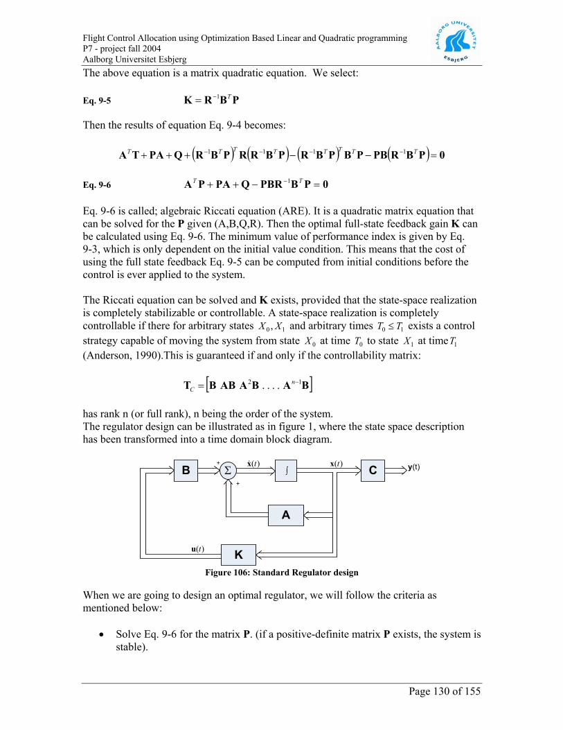
Flight Control Allocation using Optimization Based Linear and Quadratic programming P7 - project fall 2004 Aalborg Universitet Esbjerg The above equation is a matrix quadratic equation. We select: Eq. 9-5 PBRK T1−= Then the results of equation Eq. 9-4 becomes:
( ) ( ) ( ) ( ) 0PBRPBPBPBRPBRRPBRQPATA =−−+++ −−−− TTTTTTTT 1111 Eq. 9-6 0PBPBRQPAPA =−++ − TT 1
Eq. 9-6 is called; algebraic Riccati equation (ARE). It is a quadratic matrix equation that can be solved for the P given (A,B,Q,R). Then the optimal full-state feedback gain K can be calculated using Eq. 9-6. The minimum value of performance index is given by Eq. 9-3, which is only dependent on the initial value condition. This means that the cost of using the full state feedback Eq. 9-5 can be computed from initial conditions before the control is ever applied to the system. The Riccati equation can be solved and K exists, provided that the state-space realization is completely stabilizable or controllable. A state-space realization is completely controllable if there for arbitrary states and arbitrary times T10 , XX 10 T≤ exists a control strategy capable of moving the system from state at time T to state at timeT (Anderson, 1990).This is guaranteed if and only if the controllability matrix:
0X 0 1X 1
[ ]BABAABBT 12 .... −= n
C has rank n (or full rank), n being the order of the system. The regulator design can be illustrated as in figure 1, where the state space description has been transformed into a time domain block diagram.
CΣ
A
B y(t))(tx+
+
∫)(tx
K)(tu
Figure 106: Standard Regulator design
When we are going to design an optimal regulator, we will follow the criteria as mentioned below:
• Solve Eq. 9-6 for the matrix P. (if a positive-definite matrix P exists, the system is stable).
Page 130 of 155

Flight Control Allocation using Optimization Based Linear and Quadratic programming P7 - project fall 2004 Aalborg Universitet Esbjerg
• Substitute the matrix P into Eq. 9-5. The resulting matrix K is the optimal matrix. If the matrix A-BK is stable, the present methods give the correct result.
9.1.1. Solving Quadratic Regulator Problem with Matlab We use the MATLAB lqr(A,B,Q,R) command to solve the continuous-time, linear quadratic regulator problem and the Riccati equation. This command calculates the optimal feedback gain matrix K such that the feedback control law:
)()( tt Kxu −= that minimizes the performance index:
( )dtJT
T
TT∫∞=
=
+=0
RuuQxx
Subject to the constrained equation:
BuAxx += The other command in matlab is:
[ ] ),,,(,, RQAEPK Blqr= Then the command returns the gain K, eigenvalue vector E, and matrix P, the unique positive-definite solution to the Riccati equation:
0QPBPBRPAPA =+−+ − TT 1 If matrix A-BK is a stable matrix, such a positive-definite solution P always exists. The eigenvalue vector E gives the closed-loop poles of A-BK.
9.1.2. Controllable The system is controllable, if all the closed-loop poles may assigned to the desired locations by selection of K. Controllability means that the control input u(t) independently affects all the systems modes
[ ]BABAABBTc n 12 .... −=
Page 131 of 155
Flight Control Allocation using Optimization Based Linear and Quadratic programming P7 - project fall 2004 Aalborg Universitet Esbjerg Tc is controllability matrix. The system is controllable if Tc has full rank of n, and if Tc has n linearly independent columns.
9.1.3. Stabilizability and Detectability A system (A,B,C) is stabilizable if there exists a matrix K, so that A-BK is stable (i.e. it has the eigenvalues in the stability region). The system is detectable if a matrix L exists, so that A-LC is stable. A controllable system is always stabilizable. An observable system is always detectable.
9.1.4. Conditions for convergence of the LQ solution algorithm There exists a gain K such Ac is stable. If this is reality, we call the system output stabilizable. The output matrix C has full row rank p. Control weighting matrix R is positive definite. (i.e. all eigenvalues greater than zero, which implies non-singularity; denoted R > 0). This means that all the control inputs should be weighted in the performance index (PI). Weighting matrix Q is positive definite ( ) and (0≥Q AQ , ) is detectable. That is, the observability matrix polynomial
−
−=
Q
AISsO )(
has full rank n, for all values of the complex variable s not constrained in the left-half plane. If these conditions is true, the algorithm finds an output-feedback gain that stabilizes the plant and minimizes the performance index (PI). The detectability condition means that any unstable system modes must be observable in the performance index (PI). Then if PI is bounded, which it is if the optimization algorithm is successful, signal associated with the unstable modes must go to zero as t becomes large, that is, they are stabilized in the closed-loop system.
9.1.5. System description We will consider linear systems of the form:
uBAxx u+= Cxy =
Page 132 of 155

Flight Control Allocation using Optimization Based Linear and Quadratic programming P7 - project fall 2004 Aalborg Universitet Esbjerg
Where nR∈x is the system state, is the control input, y is the system output to be controlled, and is stabilizable. We assume x to be measured so that full state information is available.
mR∈u pR∈( uBA, )
Assume now that rank This implies that B can be factorized as: ( ) .mku <=B u
BBB vu =
Where and B With this, an alternative system description is given by: knv R ×∈B .mkR ×∈
vBAxx v+=
Buv = Cxy =
Where can be interpreted as the total control effort produced by the actuators. We will refer to v as the virtual control input.
kR∈v
Since B (and also Bmk < u) has null space of dimension km − in which u can be perturbed without affecting the system dynamics. This is the type of actuator redundancy that is typically considered in control allocation applications. For simplicity, we will restrict ourselves to the case k i.e, when the number if virtual control inputs equals the number of variables to be controlled.
,p=
9.1.6. The optimal Linear Quadratic control The design problem is now to select the feedback gain K that minimizes J subject to dynamic constraints, which means that the performance index J should be minimized. This is done by finding a control input u(t) such that the control input drives the state variable to zero when time goes to infinity and achieved output equal to commanded or reference signal (y = r) at steady state:
x
( ) ( ) ( ) ( )( )∫∞
+=0
11min dtJ TT
uuRuxQx
Subject to ( )xKBAuBAxx uu −=+= rCx =
The block diagram, Figure 107 is a detail description of Figure 104. In this diagram we
have a feedforward and feedback controller in the system.
Page 133 of 155

CΣr(t)
A
B y(t))(tx+
+
∫)(tx
K1
Σ-
+ )(tuN Nr
)(tcu
Flight Control Allocation using Optimization Based Linear and Quadratic programming P7 - project fall 2004 Aalborg Universitet Esbjerg
Figure 107: Feedforward and feedback control law for the redundant system
The block N in Figure 107 is a Feed-forward controller and K1 is a Feedback controller. Feed-forward calculation is a static gain of the closed-loop related to the tracking problem. The computation of Feedback controller is mainly based on chapter 1.2 (Linear Quadratic Regulator) and Feed-forward computation is based on Glad (2000, chapter 9.2) and Härkegaard (2003, chapter 10). When the system has more inputs than or equal to the outputs variables to be controlled, it needs a feed-forward controller to track the input. The static gain N matrix can be expressed in following equation:
( )[ ]+−−= BABKCN 1 Here + denotes pseudoinverse. Commanded input u(t) is:
)()( tt cuNru −= where the full-state feedback control law uc(t) is expressed in:
)()( 1 ttc xKu −= Where the feedback gain
11
1 PBRK Tu
−= To find the symmetric matrix P1 the stationary Riccati equation should be solved,
0QPBRBPAPPA =+−+ −1
11111
Tuu
T
Page 134 of 155

Flight Control Allocation using Optimization Based Linear and Quadratic programming P7 - project fall 2004 Aalborg Universitet Esbjerg
9.1.7. The optimal Linear Control with Control Allocator
CΣr(t)
A
B y(t))(tx+
+
∫)(tx
K2
Σ-
+ )(tvN Nr
)(tcv
Control )(tuAllocation
Figure 108: Feedforward and feedback control law for the redundant system with allocator
In this design we use the system description ( )2 and determine the virtual control input by solving: ( )tv
( )∫∞
+0
22min dtTT
vvRvxQx
Where 022 ≥= TQQ
is positive semi-definite,
022 >= TRR is positive definite, is detectable, and x, v solve: ( 2,QA )
rCxBAx
==+ 0v
Then determine the control input ( )tu by solving:
uu
min
Subject to vBu = In this case there is no need to minimize the scalar quantity v at steady state because the equation has a unique solution due to the dimension of v is same as the dimension of y.
vRT2
Then optimal control law becomes as;
)()( tt Svu = where:
Page 135 of 155

Flight Control Allocation using Optimization Based Linear and Quadratic programming P7 - project fall 2004 Aalborg Universitet Esbjerg
[ ]+= BS The optimal virtual control input is given by;
ct uNrv −=)( where:
)()( 2 ttc xKu −= this matrix static gain N can be expressed in following equation,
( )[ ] 11 −−−= vv BAKBCN Since N is a square we get +−+ == BSNN 1 according to lemma 1. The feedback gain K2 for design 2 can be expressed by the following equation. In this equation Bv was used instead of Bu:
21
22 PBRK Tv
−= To solve feedback gain K2, the symmetric matrix P2 should be found first. This is done by solve Riccati equation:
0PBRBPQAPPA =−++ −2
122222
Tvv
T
9.1.8. Flight Control example with ADMIRE benchmark In this design example section we will demonstrate the theory described in the previous using a flight control example. The flight control example used here is the ADMIRE model. We consider a low speed flight case, Mach 0.5 and altitude 1000 m. In this situation the efficiency of control surfaces is very poor, which means that there possible to occur actuator saturation in certain positions. The subsystem of ADMIRE described by the following state-space model.
)()()( ttt uuBAxx +=
)()()( ttt DuCxy +=
Page 136 of 155

Where nR∈x system state, u commanded control input, . mR∈ pR∈y nnR ×∈A system matrix, mnR ×∈B input matrix, C output matrix and np×R∈ mpR ×∈D is the direct transmission matrix. nR∈x and y are the state representation matrix and y the output observation matrix respectively.
pR∈ )t(
Flight Control Allocation using Optimization Based Linear and Quadratic programming P7 - project fall 2004 Aalborg Universitet Esbjerg
r
x
yδuv Control
surfaceControl
AllocatorControl
lawSystem
(A,B)
Figure 109: Control law and control allocation for over actuator system with reference input
The aircraft data for the subsystem is from the linearized ADMIRE model, where the desired states in this example are
[ ]Trqpt βα=)(x
where the state variables are α = angle of attack, β = angle of sideslip, p = roll angular rate, p = pitch angular rate, and r =yaw angular rate. The angle of attack and angle of sideslip is measure in unit (degree), whereas the roll, pitch, and yaw is measured in the unit degrees per second (deg/s). The seven control surfaces for the Admire model as depicted in chapter 2, has a first order dynamics with a time constant of 0.05 s. The transfer functions for all seven control surface becomes as,
( ) ( )•• += u
s 2020δ
where and represents actual and commanded control input of right and left canards, right outer and right inner elevons, left inner and outer elevons, and rudder. The all control surface deflections are measured in degrees.
( )•δ ( )•u
( ) [ ]Trloelierieroelcrct δδδδδδδ=• )(δ
( ) [ ]Trloelierieroelcrc uuuuuuut =• )(u Actuator position constraints are given by:
[ ]T30303030302525max =δ
[ ]T30303030305555min −−−−−−−=δ
Page 137 of 155

Flight Control Allocation using Optimization Based Linear and Quadratic programming P7 - project fall 2004 Aalborg Universitet Esbjerg The commanded output variables are the angle of attackα , side-slip β and roll rate p. Then the output matrix becomes as,
[ ]Tpt βα=)(y
System matrix A and input matrix Bu1 for the subsystem:
=
2127000939070760005057000030062212
61760099680513010096610022150117900
09778000137054320
. - . -. . - . -. . . -. - . - . . -
. . .-
A
8823009440186101861009440261502615000240462808107081070462808266082660487112849295741957412849260130601300287000240009500095000240006300063000040031800548005480031800035000350
1
. -. . . -. -. .-
. . -. -. -. -. . . . . . -. -. -. . . -. -. . . .-
. . -. -. -. -. .
= uB
The input matrix Bu1 is ganged, which means that the right canards (u ) and left canards ( ) is ganged together, right outer elevon (u ) and right inner elevon ( ) is ganged together, right inner elevon ( ) and left outer elevon (u ) is ganged together and rudder ( u ) was not ganged, because there is only one rudder ( ). Then the ganged input matrix B
rc
lcu roe rieu
rieu loe
r ruu becomes as follows,
88230280502805000024027351273516532148711242342423400287001190011900
00040086600866000690
= u
. -. . - . . -. -. . . . - . . -.
. . -. -.
B
The output matrix C and the direct transmission matrix D is given below. In this case, we will measure the responses of angle of attack (α ), sideslip ( β ), and roll rate (p), therefore, ones in diagonal entries of C matrix. All The entries of the D matrix are zeros.
001000001000001
= C
Page 138 of 155

Flight Control Allocation using Optimization Based Linear and Quadratic programming P7 - project fall 2004 Aalborg Universitet Esbjerg
000000000000
= D
For the simulation we use n×n quadratic system matrix A and n×m ganged input matrix Bu. The state variable equation ( )tx and output equation for the open-loop system yields,
)(ty
⋅
+
⋅
=
r
le
re
c
uuuu
rqpt
0.8823- 0.2805 0.2805- 0 0.0024 1.2735- 1.2735- 1.6532 1.4871 4.2423 4.2423- 0 0.0287 0.0119- 0.0119 0 0.0004 0.0866- 0.0866- 0.0069
0.2127- 0 0.0939- 0.7076 0 0 0.5057- 0 0.0030- 2.6221
0.6176 0 0.9968- 10.5130- 0 0.9661- 0 0.2215 0.1179- 0
0 0.9778 0 0.0137 0.5432-
)(βα
x
⋅
+
⋅
=
r
le
re
c
uuuu
rqpt
0 0 0 00 0 0 00 0 0 0
0 0 1 0 00 0 0 1 00 0 0 0 1
)(βα
y
We check the open-loop stability by the system matrix A. Then we get the open-loop systems pole placement, damping ratio and natural frequency using MATLAB command damp; States x(t) Eigenvalue Damping (ζ) Natural frequency
(wn) (rad/s) Angle of attack, α (dutch mode)
1.08 -1.00 1.0800
Angle of sideslip, β (dutch mode)
-0.3180 + 1.7000i 0.1840 1.7300
Roll angular rate, p (short period mode)
-0.3180 - 1.7000i 0.1840 1.7300
Pitch angular rate, q (short mode)
-0.6920 1.00 0.6920
Yaw angular rate, r -2.1300 1.00 2.1300 It seems that the system has an unstable pole at 1.08 for angle of attack and insufficient damping for angle of attack, pitch rate, and yaw rate. Since unstable pole and insufficient damping, the system requires a feedback gain K. Therefore for we use optimal LQ control with feedback design.
Page 139 of 155

Flight Control Allocation using Optimization Based Linear and Quadratic programming P7 - project fall 2004 Aalborg Universitet Esbjerg For computation of feedback gain K it is necessary to select the performance index weighting matrix Q and R as discussed in chapter 1.2. Then we can compute the optimal gain K. First will we discuss the choice of Q. It is desired to obtain good stability of the dutch mode, so that and should be weighted in the performance Index (PI) by factors q2α 2β dr. To obtain good stability of short period mode, which in closed-loop will consist primarily of p and q, we may weight and in the PI by factors q2p 2q sp. The roll mode consists of r, so that 2r should be weighted in the PI by factors qr, to have good stability criteria, then we have:
[ ]rspspdrdr qqqqqdiag=Q As far as the R matrix goes, it is generally satisfied to select R as:
IR ρ=
where I is the identity matrix and ρ a scalar design parameter. After few trials, we obtained a good result using
2000001000001000000200000020
= Q
1.000001.000001.000001.0
=R
For this selection, the solution for the symmetric matrix P1 obtained from the continuous-time Riccati equation, the optimal feedback gain K1 was:
0QPBRBPAPPA =+−+ −1
11111
Tuu
T
0.60310.00020.0197-1.0139-0.00050.00020.14420.0000-0.00060.31340.0197-0.0000-0.16000.04290.0001-1.0139- 0.00060.04298.86410.00940.00050.31340.0001-0.00944.8288
= P1
Page 140 of 155

Flight Control Allocation using Optimization Based Linear and Quadratic programming P7 - project fall 2004 Aalborg Universitet Esbjerg
11
1 PBRK Tu
−=
K1
=
5.9053-0.00322.564712.12810.02420.97472.1080-6.72562.0937-8.1749-0.9798- 2.1072-6.7251-2.06258.1697-
0.00282.40530.0003-0.01035.5136
Now we can check the closed-loop stability again with the stable closed-loop matrix . The closed-loop dynamic matrix computed as below, 1KBAA ucl −=
= Acl
5.9711-0.00301.6040-12.57400.02280.00329.8503-0.0049-0.0889-27.3078-1.10800.0013-61.8726-10.9165-0.0142-0.7734-0.0001-0.30800.5154-0.0008-0.00190.59620.0010-0.00611.9967-
We check the closed-loop stability again by the system matrix Acl. Then we get the closed-loop systems poles, damping ratio and natural frequency using the MATLAB command “damp”: States, x(t) Eigenvalues Damping (ζ) Natural Frequency (wn)
in (rad/s) Angle of attack, α (dutch mode)
-0.989 + 1.40i 0.5760 1.72
Angle of sideslip, β (dutch mode)
-0.989 - 1.40i 0.5760 1.72
Roll angular rate, p (short period mode)
-1.81 + 0.3440i 0.9820 1.84
Pitch angular rate, (short mode)
q -1.81 - 0.3440i 0.9820 1.84
Yaw angular rate, r -2.34 1.00 2.34 It seems that all the poles are in the stability region and is moved further to left-hand side of the S-plane with the slowest time constant, τ = 1/2.34 = 0.42 sec.
Page 141 of 155

Flight Control Allocation using Optimization Based Linear and Quadratic programming P7 - project fall 2004 Aalborg Universitet Esbjerg
9.1.9. Simulation results for Design 1
Figure 110: Output response of angle of attack, side-slip and roll rate
We set the reference input, angle of attack to 5 degrees, side-slip to 10 deg, and roll to rate 20 deg/sec. Step input occurs start at t=2 sec. and it should be settled at the desired commanded input at steady state. The Figure 110 depicted the output response of these three variables. As it can be seen in Figure 110, the angle of attack and roll rate settled at 5 degrees and 20 degrees/sec after 1 second, respectively. Side-slip response settled at 10 after 1.5 seconds.
9.1.10. Design 2 The design model used here is
vBAxuBAxx vu +=+= Buv =
As described in section 1.2.5 the matrix Bu was factorized into two matrices Bv and B. where B . Matrix B contains the last three rows of BBBvu =
Buv =u. The virtual control
input, , contains the angular acceleration in roll, pitch, and yaw produced by the control surfaces.
Page 142 of 155

Flight Control Allocation using Optimization Based Linear and Quadratic programming P7 - project fall 2004 Aalborg Universitet Esbjerg
100010001000000
= Bv
8823028050280500002402735127351653214871124234242340
. -. . - . . -. -.. . . -
= B
The same weighting matrices Q2=Q1 and R2=R1 as in design 1 is used in this example. Then the solution for the symmetric matrix P2 from continuous-time Riccati equation and optimal feedback gain K2 is:
0PBRBPQAPPA =−++ −2
122222
Tvv
T
=
0.67910.00000.0212- 1.2915-0.0009-0.00000.17590.0000-0.00140.52570.0212-0.0000-0.15990.03970.00001.2915-0.00140.03979.42310.01420.0009-0.52570.00000.01425.7451
2P
21
22 PBRK Tv
−=
=
6.12930.0036- 1.509611.6616- 0.0194-0.0138-10.51530.00550.113831.41750.8381-0.002460.87241.38230.0192
K 2
Nbar can be calculated by equation ( )[ ] 11 −−−= vv BAKBCN , and becomes a 3×3 square matrix.
=
3.057513.1432- 0.0214-0.00230.0359- 34.9179
61.535512.07290.0206Nbar
9.1.11. Simulations result for design 2 In this simulation will we test the output variables settled at a desired position in steady state. In the second test, will we analyse how good the control surfaces produce the
Page 143 of 155

Flight Control Allocation using Optimization Based Linear and Quadratic programming P7 - project fall 2004 Aalborg Universitet Esbjerg desired moment. In this test we will not include the constraints. In the final test we will include constraints and consider the control surfaces according to the boundaries, when they produce the desired moment.Design 2 considers the system without constraints
Figure 111: Output response for design 2
As in design 1, the reference input, angle of attack is set to 5 degrees, sideslip to 10 degrees, and roll rate to 20 deg/sec. The step input is given at t=2 sec. Figure 111 shows the response of the angle of attack, sideslip, and roll rate. As it can be seen as in Figure 111 the angle of attack and roll rate settles at 5 degrees and 20 deg/sec after 1 second. There is small tracking error in angle of attack. Sideslip settled at 10 degrees after 1.5 seconds. From these two design approaches we can conclude that design 1, without control allocator and design 2, with control allocator, gives exactly same response. Control inputs The following four figures illustrate the control surfaces deflection for the aircraft response. In this test constraints are not included. However, it can be clearly seen from the figures that the control surfaces exceeds the maximum and minimum constraints in some cases.
Page 144 of 155

Flight Control Allocation using Optimization Based Linear and Quadratic programming P7 - project fall 2004 Aalborg Universitet Esbjerg
Figure 112: the control surfaces deflections
Another interesting point here is that have the control surfaces produced the desired moment v. It can be confirmed by taking the produced moment by the control surfaces multiply by the control effectiveness matrix B, which means Buv = .
Page 145 of 155

Flight Control Allocation using Optimization Based Linear and Quadratic programming P7 - project fall 2004 Aalborg Universitet Esbjerg
Figure 113: The desired moment v
Figure 114: Achieved moment v
Figure 114 shows the desired moment and the achieved moment. There is no difference between these two figures. This means that the control surfaces has achieved the desired moment. As mentioned before the control surfaces exceed their maximum and minimum boundaries. Therefore is this an inadequate method. In the following four figures illustrates the control surfaces deflection for aircraft response. In this test constraints included and cascaded generalized psedoinverse algorithm was used. Anyway, it can be clearly seen from the figures the control surfaces are into their maximum and minimum constraints.
Page 146 of 155

Flight Control Allocation using Optimization Based Linear and Quadratic programming P7 - project fall 2004 Aalborg Universitet Esbjerg
Figure 115: control surfaces deflections after included constraints
Figure 116: Desired moment v
Page 147 of 155

Flight Control Allocation using Optimization Based Linear and Quadratic programming P7 - project fall 2004 Aalborg Universitet Esbjerg
Figure 117: Achived moment v
Figure 117 illustrate the desired moment and the achieved moment for design 2. The figures are almost same. There are only small differences between these two figures. Output response for this design is depicted below:
Figure 118: output response for design 2 after constrints in allocator
Using the allocation algorithm in our LQR design reveals that the system has almost the same response, while also being more real-world applicable since the position constraints
Page 148 of 155

Flight Control Allocation using Optimization Based Linear and Quadratic programming P7 - project fall 2004 Aalborg Universitet Esbjerg is considered. The settling times for all three variables are very close to the settling times in the non-constrained case.
9.2. Summery LQR design for flight control is a powerful tool. LQR on its own can distribute the control effect to the redundant control surfaces of the aircraft but it lacks the possibility of regarding constraints in design 1. Using design 2 it is possible to include a control allocation algorithm into the LQR designs, thereby making it adhere to the constraints of the system’s actuators. The choice of algorithm depends on the goal of the controller, and the three tested algorithms have their different weaknesses and strengths. In order to choose the optimal algorithm for LQR design 2 the weaknesses and strengths of the algorithms must be considered.
Page 149 of 155

Flight Control Allocation using Optimization Based Linear and Quadratic programming P7 - project fall 2004 Aalborg Universitet Esbjerg
10. Appendix A. Lemma 1. The least squares problem
Min xxx T=2 Subject to yAx =
Where
( ) 1−+ = TT AAAA is the pseudoinverse of . A
10.1. Symmetric matrices
A symmetric matrix such as matrix A given by AAT = if this is true it is necessarily square. Its main diagonal entries are arbitrary, but its other entries occur in pairs- on opposite sides of the main diagonal.
10.1.1. Example: Symmetric matrices,
−
=30
01A
−
=30
01TA
AAT = is symmetric
−−
−=
780851010
B
−−
−=
780851010
TB
BBT = is symmetric
For example, XX T is called Quadratic forms. A quadratic form on nR function Z defined on nR whose value at a vector x in nR can be computed by and expressed of the form, ( )X = AXXZ T , where A is an symmetric matrix. Matrix A is then called the “matrix of the quadratic form”.
nn ×
The simplest example of a nonzero quadratic form is
Page 150 of 155

Flight Control Allocation using Optimization Based Linear and Quadratic programming P7 - project fall 2004 Aalborg Universitet Esbjerg
( )2XIXXxZ T == .
10.1.2. Example1.
=
2
1
xx
X
Compute AXX T for the following matrices.
a) b)
=
3004
A
−
−=
7223
B
a) [ ]
=
2
121 30
04xx
xxAXX T
= [ ] 22
21
2
121 34
34
xxxx
xx +=
b) There are two -2 entries in A.
[ ] [ ]
+−−
=
−
−=
21
2121
2
121 72
237223
xxxx
xxxx
xxAXX T
= ( ) ( )212211 7223 xxxxxx +−+− = 3 2
2122121 722 xxxxxx +−−
= 3 2221
21 74 xxxx +−
The presence of in the quadratic form in example 214 xx− ( )b1 is due to the -2 entries off the diagonal matrix. In Example ( )a1 has no cross-product term. 21xx
10.1.3. Example 2
For X in let ,3R
( ) .8235 322123
22
21 xxxxxxxxQ +−++=
then we will write this in quadratic form as:
.AXX T Solution:
Page 151 of 155

Flight Control Allocation using Optimization Based Linear and Quadratic programming P7 - project fall 2004 Aalborg Universitet Esbjerg
The coefficients go on the diagonal of A. To make A symmetric, the coefficient of for
23
22
21 ,, xxx
jxix ji must split evenly between the≠ ( )ji, , and ( )ij, entries in A. The coefficient of is 0. It is readily checked that: 31 xx
( ) [ ]
−
−==
3
2
1
321
24043½0½5
xxx
xxxAXXXQ T
10.1.4. Example 3 Let
( ) .58 2221
21 xxxxXQ −−=
Compute the value of Q for (X )
−=
13
X , and
− 31
Solution:
( ) ( ) ( )( ) ( ) 281513831,3 22 =−−−−=−Q ( ) ( )( ) ( ) 162522822,2 22 =−−−−=−Q ( ) ( ) ( )( ) ( ) .203531813,1 22 −=−−−−=−Q
Page 152 of 155

Flight Control Allocation using Optimization Based Linear and Quadratic programming P7 - project fall 2004 Aalborg Universitet Esbjerg
11. Aircraft nomenclature State variables Symbol: unit Definition α rad angle of attack β rad angle of sideslip γ rad flight path angle u m/s longitudinal velocity v m/s lateral velocity w m/s normal velocity VT m/s total velocity p rad/s roll rate q rad/s pitch rate r rad/s yaw rate pN m position north pE m position east h m altitude φ rad roll angle θ rad pitch angle ψ rad yaw angle nz g load factor, normal accel. nzp g pilot load factor
Coordinate frames Symbol Defintion
( )iiii zyxe ˆ,ˆ,ˆ= inertial, Earth-fixed frame ( )bbbb zyxe ˆ,ˆ,ˆ= body-fixed frame ( )wwww zyxe ˆ,ˆ,ˆ= wind-axes frame
Control surface deflections Symbol unit Definition
rcδ rad right canard
lcδ rad left canard
roeδ rad right outer elevon
rieδ rad right inner elevon
loeδ rad left outer elevon
lieδ rad left inner eleveon
rδ rad rudder
Forces and moments Symbol unit Definition g m/s2 gravitational acceleration
Page 153 of 155

Flight Control Allocation using Optimization Based Linear and Quadratic programming P7 - project fall 2004 Aalborg Universitet Esbjerg FT N engine thrust force
DSCqD = N drag force
lSCqL = N lift force
YSCqY = N side force
lSbCqL = Nm rolling moment
mCcSqM = Nm pitching moment
nSbCqN = Nm yawing moment
Aircraft data Symbol unit Definition m kg aircraft mass
−
−=
zxz
y
xzx
III
III
000
0
kgm2
aircraft inertial matrix
S m2 wing platform area b m wing span c m mean aerodynamic chord zTP m zb-position of engine thrust point xP m xb-position of the pilot
Atmosphere Symbol unit Definition p kg/m3 air density q N/m2 dynamic pressure
Page 154 of 155

Flight Control Allocation using Optimization Based Linear and Quadratic programming P7 - project fall 2004 Aalborg Universitet Esbjerg
Page 155 of 155
12. References Chapra, Steven C. & Canale, Raymond P. 2002, Numerical methods for engineers, McGraw-Hill, New York. Lay, David C. 2000, Linear algebra and its applications, Addison-Wesley, U.S. Härkegård, Ola 2003 Backstepping and control allocation with applications to flight control, Ph. D. thesis, Linköping University, Linköping Bodson, Marc 2002 ‘Evaluation of optimization methods for control allocation’, Journal of guidance, control and dynamics, vol. 25, no.4, pp. 703-711 Bordignon, K.A 1996 Constrained control allocation for systems with redundant control effectors, Ph. D. thesis,Virginia Polytechnic Institute, Virginia. L. Stevens, Brian & L. Lewis, Frank 2003, Aircraft control and simulation, Wiley, New Jersey. Glad, Torkel & Ljung, Lennart 2000 Control theory: multivariable and nonlinear methods, Taylor & Francis, New York. Anderson, Brian D.O. & Moore, John B. 1990, Optimal control: Linear quadratic methods, Prentice Hall, New Jersey. Ogata, Katsuhiko 2002, Modern control engineering, Prentice Hall, New Jersey. Mathworks, 2002, MATLAB, ver. 6.5, computer program, The MathWorks Inc., 24 Prime Park Way, Natick, MA 01760-1500 USA.
13. Appendix B.
14. Additional reading
15. Matlab code