Fixed/Random effects (R) - Princeton University

Getting Started in Fixed/Random Effects Models

using R(ver. 0.1-Draft)

Oscar Torres-ReynaData [email protected]

http://dss.princeton.edu/training/

http://dss.princeton.edu/training/Panel101.pdf�

http://cran.r-project.org/web/packages/plm/vignettes/plm.pdf�

RANDOM-EFFECTS MODEL(Random Intercept, Partial Pooling Model)

Random effects (using plm)

> random <- plm(y ~ x1, data=Panel, index=c("country", "year"), model="random")> summary(random)

Oneway (individual) effect Random Effect Model (Swamy-Arora's transformation)

Call:plm(formula = y ~ x1, data = Panel, model = "random", index = c("country",

"year"))

Balanced Panel: n=7, T=10, N=70

Effects:var std.dev share

idiosyncratic 7.815e+18 2.796e+09 0.873individual 1.133e+18 1.065e+09 0.127theta: 0.3611

Residuals :Min. 1st Qu. Median Mean 3rd Qu. Max.

-8.94e+09 -1.51e+09 2.82e+08 5.29e-08 1.56e+09 6.63e+09

Coefficients :Estimate Std. Error t-value Pr(>|t|)

(Intercept) 1037014284 790626206 1.3116 0.1941x1 1247001782 902145601 1.3823 0.1714

Total Sum of Squares: 5.6595e+20Residual Sum of Squares: 5.5048e+20R-Squared : 0.02733

Adj. R-Squared : 0.026549 F-statistic: 1.91065 on 1 and 68 DF, p-value: 0.17141

# Setting as panel data (an alternative way to run the above model

Panel.set <- plm.data(Panel, index = c("country", "year"))

# Random effects using panel setting (same output as above)

random.set <- plm(y ~ x1, data = Panel.set, model="random")summary(random.set)

Random effects option

Outcome variable

Predictor variable(s)

Panel setting

n = # of groups/panels, T = # years, N = total # of observations

Pr(>|t|)= Two-tail p-values test the hypothesis that each coefficient is different from 0. To reject this, the p-value has to be lower than 0.05 (95%, you could choose also an alpha of 0.10), if this is the case then you can say that the variable has a significant influence on your dependent variable (y)

If this number is < 0.05 then your model is ok. This is a test (F) to see whether all the coefficients in the model are different than zero.

Interpretation of the coefficients is tricky since they include both the within-entity and between-entity effects. In the case of TSCS data represents the average effect of X over Y when X changes across time and between countries by one unit.

For the theory behind random effects please see: http://dss.princeton.edu/training/Panel101.pdf

14


FIXED OR RANDOM?

Fixed or Random: Hausman test

To decide between fixed or random effects you can run a Hausman test where the null hypothesis is that the preferred model is random effects vs. the alternative the fixed effects (see Green, 2008, chapter 9). It basically tests whether the unique errors (ui) are correlated with the regressors, the null hypothesis is they are not.

Run a fixed effects model and save the estimates, then run a random model and save the estimates, then perform the test. If the p-value is significant (for example <0.05) then use fixed effects, if not use random effects.

16

> phtest(fixed, random)

Hausman Test

data: y ~ x1 chisq = 3.674, df = 1, p-value = 0.05527alternative hypothesis: one model is inconsistent

If this number is < 0.05 then use fixed effects

For the theory behind fixed/random effects please see: http://dss.princeton.edu/training/Panel101.pdf


OTHER TESTS/ DIAGNOSTICS

Testing for time-fixed effects

18

> library(plm)> fixed <- plm(y ~ x1, data=Panel, index=c("country", "year"), model="within")> fixed.time <- plm(y ~ x1 + factor(year), data=Panel, index=c("country", "year"), model="within")> summary(fixed.time)Oneway (individual) effect Within Model

Call:plm(formula = y ~ x1 + factor(year), data = Panel, model = "within",

index = c("country", "year"))



-7.92e+09 -1.05e+09 -1.40e+08 1.48e-07 1.63e+09 5.49e+09


x1 1389050354 1319849567 1.0524 0.29738 factor(year)1991 296381559 1503368528 0.1971 0.84447 factor(year)1992 145369666 1547226548 0.0940 0.92550 factor(year)1993 2874386795 1503862554 1.9113 0.06138 .factor(year)1994 2848156288 1661498927 1.7142 0.09233 .factor(year)1995 973941306 1567245748 0.6214 0.53698 factor(year)1996 1672812557 1631539254 1.0253 0.30988 factor(year)1997 2991770063 1627062032 1.8388 0.07156 .factor(year)1998 367463593 1587924445 0.2314 0.81789 factor(year)1999 1258751933 1512397632 0.8323 0.40898 ---Signif. codes: 0 ‘***’ 0.001 ‘**’ 0.01 ‘*’ 0.05 ‘.’ 0.1 ‘ ’ 1



> # Testing time-fixed effects. The null is that no time-fixed effects needed

> pFtest(fixed.time, fixed)

F test for individual effects

data: y ~ x1 + factor(year) F = 1.209, df1 = 9, df2 = 53, p-value = 0.3094alternative hypothesis: significant effects

> plmtest(fixed, c("time"), type=("bp"))

Lagrange Multiplier Test - time effects (Breusch-Pagan)

data: y ~ x1 chisq = 0.1653, df = 1, p-value = 0.6843alternative hypothesis: significant effects

If this number is < 0.05 then use time-fixed effects. In this example, no need to use time-fixed effects.

Testing for random effects: Breusch-Pagan Lagrange multiplier (LM)

The LM test helps you decide between a random effects regression and a simple OLS regression.

The null hypothesis in the LM test is that variances across entities is zero. This is, no significant difference across units (i.e. no panel effect). (http://dss.princeton.edu/training/Panel101.pdf)

19Here we failed to reject the null and conclude that random effects is not appropriate. This is, no evidence of significant differences across countries, therefore you can run a simple OLS regression.

> # Regular OLS (pooling model) using plm> > pool <- plm(y ~ x1, data=Panel, index=c("country", "year"), model="pooling")> summary(pool)

Oneway (individual) effect Pooling Model

Call:plm(formula = y ~ x1, data = Panel, model = "pooling", index = c("country",

"year"))



-9.55e+09 -1.58e+09 1.55e+08 1.77e-08 1.42e+09 7.18e+09


(Intercept) 1524319070 621072624 2.4543 0.01668 *x1 494988914 778861261 0.6355 0.52722 ---Signif. codes: 0 ‘***’ 0.001 ‘**’ 0.01 ‘*’ 0.05 ‘.’ 0.1 ‘ ’ 1



> # Breusch-Pagan Lagrange Multiplier for random effects. Null is no panel effect (i.e. OLS better).

> plmtest(pool, type=c("bp"))

Lagrange Multiplier Test - (Breusch-Pagan)

data: y ~ x1 chisq = 2.6692, df = 1, p-value = 0.1023alternative hypothesis: significant effects

Testing for cross-sectional dependence/contemporaneous correlation: using Breusch-Pagan LM test of independence and Pasaran CD test

According to Baltagi, cross-sectional dependence is a problem in macro panels with long time series. This is not much of a problem in micro panels (few years and large number of cases).

The null hypothesis in the B-P/LM and Pasaran CD tests of independence is that residuals across entities are not correlated. B-P/LM and Pasaran CD (cross-sectional dependence) tests are used to test whether the residuals are correlated across entities*. Cross-sectional dependence can lead to bias in tests results (also called contemporaneous correlation).

20

No cross-sectional dependence

*Source: Hoechle, Daniel, “Robust Standard Errors for Panel Regressions with Cross-Sectional Dependence”, http://fmwww.bc.edu/repec/bocode/x/xtscc_paper.pdf

> fixed <- plm(y ~ x1, data=Panel, index=c("country", "year"), model="within")

> pcdtest(fixed, test = c("lm"))

Breusch-Pagan LM test for cross-sectional dependence in panels

data: formula chisq = 28.9143, df = 21, p-value = 0.1161alternative hypothesis: cross-sectional dependence

> pcdtest(fixed, test = c("cd"))

Pesaran CD test for cross-sectional dependence in panels

data: formula z = 1.1554, p-value = 0.2479alternative hypothesis: cross-sectional dependence

http://fmwww.bc.edu/repec/bocode/x/xtscc_paper.pdf�

Testing for serial correlation

Serial correlation tests apply to macro panels with long time series. Not a problem in micro panels (with very few years). The null is that there is not serial correlation.

21

No serial correlation

> pbgtest(fixed)Loading required package: lmtest

Breusch-Godfrey/Wooldridge test for serial correlation in panel models

data: y ~ x1 chisq = 14.1367, df = 10, p-value = 0.1668alternative hypothesis: serial correlation in idiosyncratic errors

Testing for unit roots/stationarity

22

> Panel.set <- plm.data(Panel, index = c("country", "year"))

> library(tseries)

> adf.test(Panel.set$y, k=2)

Augmented Dickey-Fuller Test

data: Panel.set$yDickey-Fuller = -3.9051, Lag order = 2, p-value = 0.01910alternative hypothesis: stationary

The Dickey-Fuller test to check for stochastic trends. The null hypothesis is that the series has a unit root (i.e. non-stationary). If unit root is present you can take the first difference of the variable.

If p-value < 0.05 then no unit roots present.

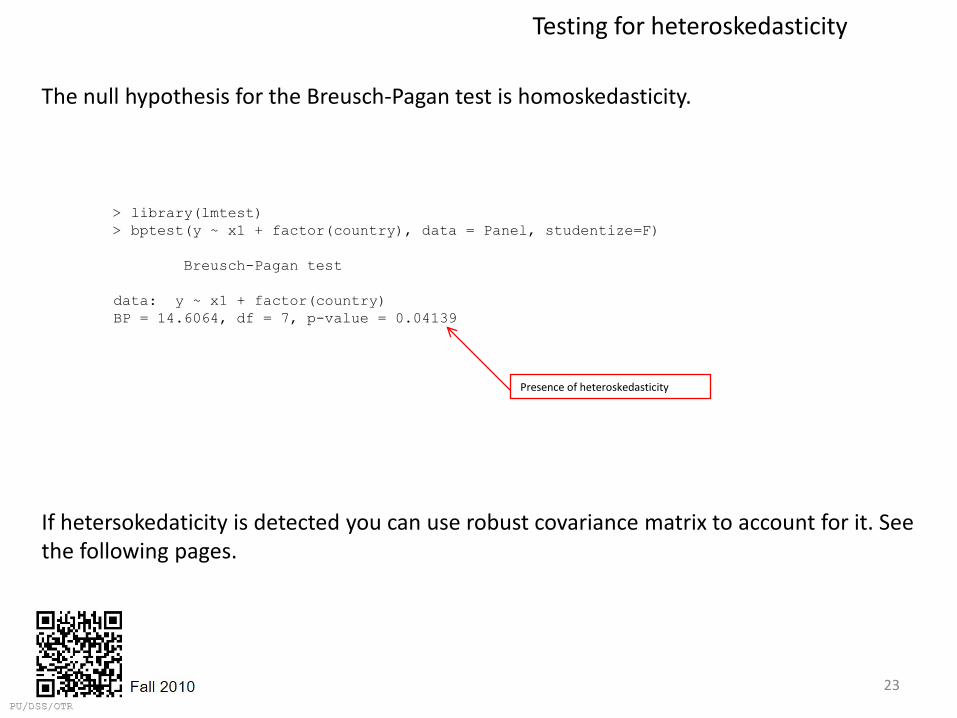
Testing for heteroskedasticity

The null hypothesis for the Breusch-Pagan test is homoskedasticity.

23

Presence of heteroskedasticity

If hetersokedaticity is detected you can use robust covariance matrix to account for it. See the following pages.

> library(lmtest)> bptest(y ~ x1 + factor(country), data = Panel, studentize=F)

Breusch-Pagan test

data: y ~ x1 + factor(country) BP = 14.6064, df = 7, p-value = 0.04139

Controlling for heteroskedasticity: Robust covariance matrix estimation (Sandwich estimator)

24

The --vcovHC– function estimates three heteroskedasticity-consistent covariance estimators:

• "white1" - for general heteroskedasticity but no serial correlation. Recommended for random effects.

• "white2" - is "white1" restricted to a common variance within groups. Recommended for random effects.

• "arellano" - both heteroskedasticity and serial correlation. Recommended for fixed effects.

The following options apply*:

• HC0 - heteroskedasticity consistent. The default.• HC1,HC2, HC3 – Recommended for small samples. HC3 gives less weight to influential

observations.• HC4 - small samples with influential observations• HAC - heteroskedasticity and autocorrelation consistent (type ?vcovHAC for more

details)

See the following pages for examples

For more details see:

• http://cran.r-project.org/web/packages/plm/vignettes/plm.pdf• http://cran.r-project.org/web/packages/sandwich/vignettes/sandwich.pdf (see page 4)• Stock and Watson 2006.• *Kleiber and Zeileis, 2008.


http://cran.r-project.org/web/packages/sandwich/vignettes/sandwich.pdf�

Controlling for heteroskedasticity: Random effects

25

> random <- plm(y ~ x1, data=Panel, index=c("country", "year"), model="random")

> coeftest(random) # Original coefficients

t test of coefficients:

Estimate Std. Error t value Pr(>|t|)(Intercept) 1037014284 790626206 1.3116 0.1941x1 1247001782 902145601 1.3823 0.1714

> coeftest(random, vcovHC) # Heteroskedasticity consistent coefficients



> coeftest(random, vcovHC(random, type = "HC3")) # Heteroskedasticity consistent coefficients, type 3



> # The following shows the HC standard errors of the coefficients

> t(sapply(c("HC0", "HC1", "HC2", "HC3", "HC4"), function(x) sqrt(diag(vcovHC(random, type = x)))))

(Intercept) x1HC0 907983029 828970247HC1 921238957 841072643HC2 925403820 847733474HC3 943438284 867137584HC4 941376033 866024033

Standard errors given different types of HC.

> fixed <- plm(y ~ x1, data=Panel, index=c("country", "year"), model="within")

> coeftest(fixed) # Original coefficients


Estimate Std. Error t value Pr(>|t|) x1 2475617827 1106675594 2.237 0.02889 *---Signif. codes: 0 ‘***’ 0.001 ‘**’ 0.01 ‘*’ 0.05 ‘.’ 0.1 ‘ ’ 1

> coeftest(fixed, vcovHC) # Heteroskedasticity consistent coefficients


Estimate Std. Error t value Pr(>|t|) x1 2475617827 1358388942 1.8225 0.07321 .---Signif. codes: 0 ‘***’ 0.001 ‘**’ 0.01 ‘*’ 0.05 ‘.’ 0.1 ‘ ’ 1

> coeftest(fixed, vcovHC(fixed, method = "arellano")) # Heteroskedasticity consistent coefficients (Arellano)



> coeftest(fixed, vcovHC(fixed, type = "HC3")) # Heteroskedasticity consistent coefficients, type 3



> # The following shows the HC standard errors of the coefficients> t(sapply(c("HC0", "HC1", "HC2", "HC3", "HC4"), function(x) sqrt(diag(vcovHC(fixed, type = x)))))

HC0.x1 HC1.x1 HC2.x1 HC3.x1 HC4.x1[1,] 1358388942 1368196931 1397037369 1439083523 1522166034

Controlling for heteroskedasticity: Fixed effects

26Standard errors given different types of HC.

References/Useful links

• DSS Online Training Section http://dss.princeton.edu/training/

• Princeton DSS Libguides http://libguides.princeton.edu/dss

• John Fox’s site http://socserv.mcmaster.ca/jfox/

• Quick-R http://www.statmethods.net/

• UCLA Resources to learn and use R http://www.ats.ucla.edu/stat/R/

• UCLA Resources to learn and use Stata http://www.ats.ucla.edu/stat/stata/

• DSS - Stata http://dss/online_help/stats_packages/stata/

• DSS - R http://dss.princeton.edu/online_help/stats_packages/r

• Panel Data Econometrics in R: the plm package http://cran.r-project.org/web/packages/plm/vignettes/plm.pdf

• Econometric Computing with HC and HAC Covariance Matrix Estimatorshttp://cran.r-project.org/web/packages/sandwich/vignettes/sandwich.pdf

27

http://dss.princeton.edu/training/�

http://libguides.princeton.edu/dss�

http://socserv.mcmaster.ca/jfox/�

http://www.statmethods.net/�

http://www.ats.ucla.edu/stat/R/�

http://www.ats.ucla.edu/stat/stata/�

http://dss/online_help/stats_packages/stata/�

http://dss.princeton.edu/online_help/stats_packages/r�


http://cran.r-project.org/web/packages/sandwich/vignettes/sandwich.pdf�

References/Recommended books

• An R Companion to Applied Regression, Second Edition / John Fox , Sanford Weisberg, Sage Publications, 2011

• Data Manipulation with R / Phil Spector, Springer, 2008

• Applied Econometrics with R / Christian Kleiber, Achim Zeileis, Springer, 2008

• Introductory Statistics with R / Peter Dalgaard, Springer, 2008

• Complex Surveys. A guide to Analysis Using R / Thomas Lumley, Wiley, 2010

• Applied Regression Analysis and Generalized Linear Models / John Fox, Sage, 2008

• R for Stata Users / Robert A. Muenchen, Joseph Hilbe, Springer, 2010

• Introduction to econometrics / James H. Stock, Mark W. Watson. 2nd ed., Boston: Pearson Addison Wesley, 2007.

• Data analysis using regression and multilevel/hierarchical models / Andrew Gelman, Jennifer Hill. Cambridge ; New York : Cambridge University Press, 2007.

• Econometric analysis / William H. Greene. 6th ed., Upper Saddle River, N.J. : Prentice Hall, 2008.

• Designing Social Inquiry: Scientific Inference in Qualitative Research / Gary King, Robert O. Keohane, Sidney Verba, Princeton University Press, 1994.

• Unifying Political Methodology: The Likelihood Theory of Statistical Inference / Gary King, Cambridge University Press, 1989

• Statistical Analysis: an interdisciplinary introduction to univariate & multivariate methods / Sam

Kachigan, New York : Radius Press, c1986

• Statistics with Stata (updated for version 9) / Lawrence Hamilton, Thomson Books/Cole, 2006

28

Fixed/Random effects (R) - Princeton University

Documents

Transcript of Fixed/Random effects (R) - Princeton University