Fixed Effects Regression

7/28/2019 Fixed Effects Regression

http://slidepdf.com/reader/full/fixed-effects-regression 1/45

Fixed effects regression methods for

longitudinal data

Paul D. Allison



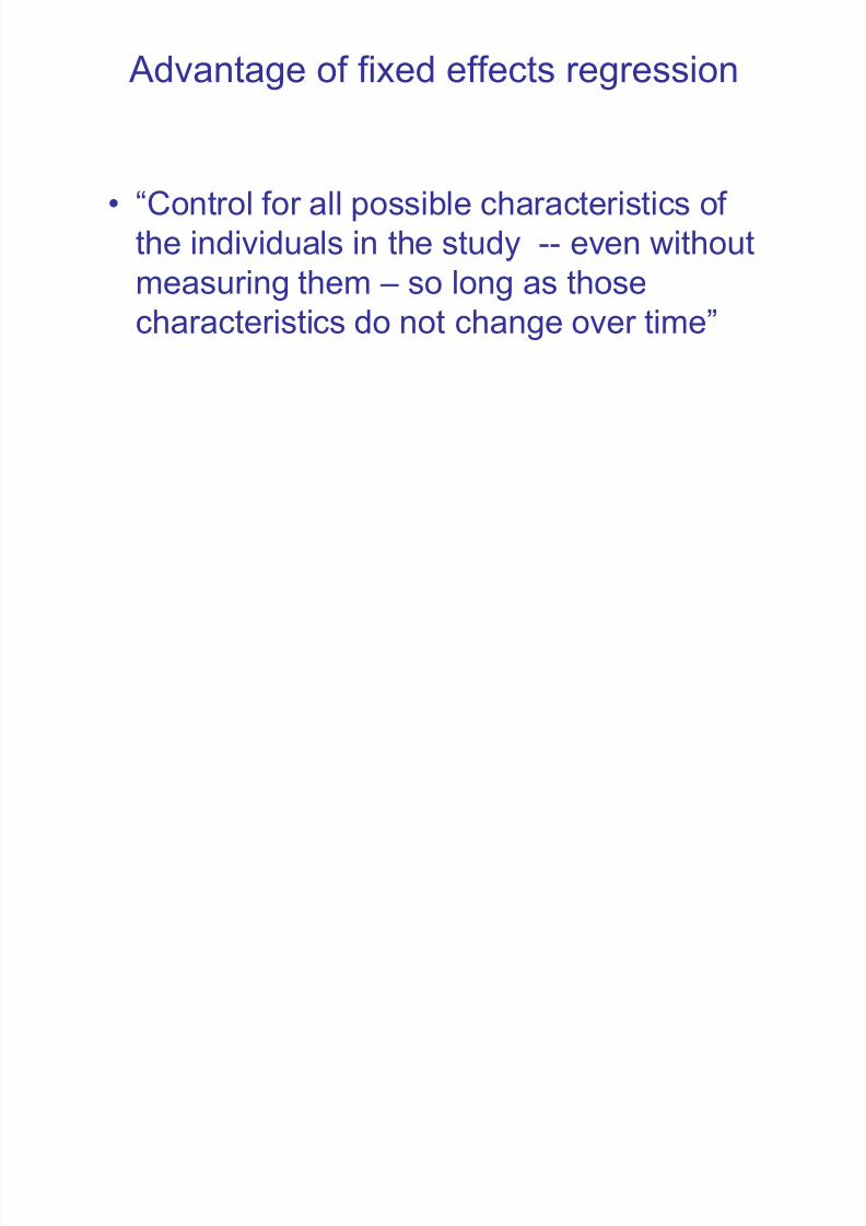
Advantage of fixed effects regression

• “Control for all possible characteristics of

the individuals in the study -- even withoutmeasuring them – so long as those

characteristics do not change over time”



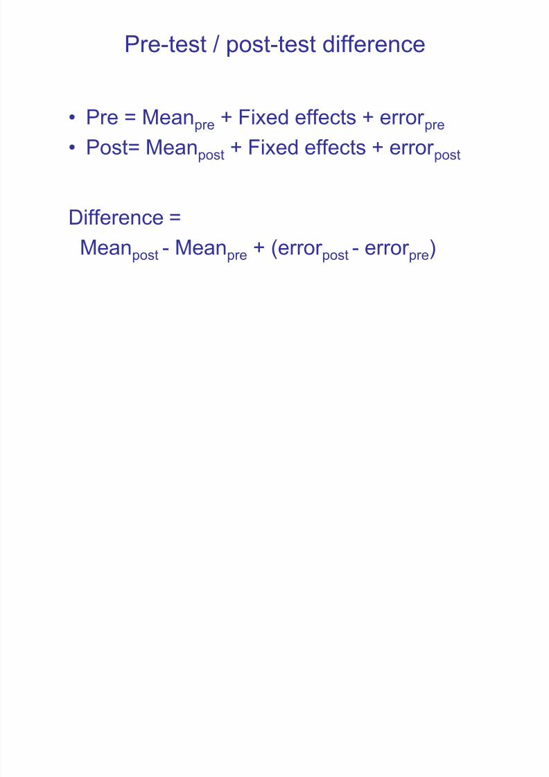
Pre-test / post-test difference

• Pre = Meanpre + Fixed effects + error pre

• Post= Meanpost + Fixed effects + error post

Difference =

Meanpost - Meanpre + (error post - error pre)



• Pre =

Meanpre + FEknown + FEunknown + error pre

• Post=Meanpost + FEknown + FEunknown + error post

Difference =Meanpost - Meanpre + (error post - error pre)

Known and unknown fixed effects (FE)



Caveat

• Fixed effects must not only be stable

characteristics of the participants over

time, but the strength of the associations

for the fixed effects must also be constantover time

• Otherwise the fixed effects must be

controlled in the analysis



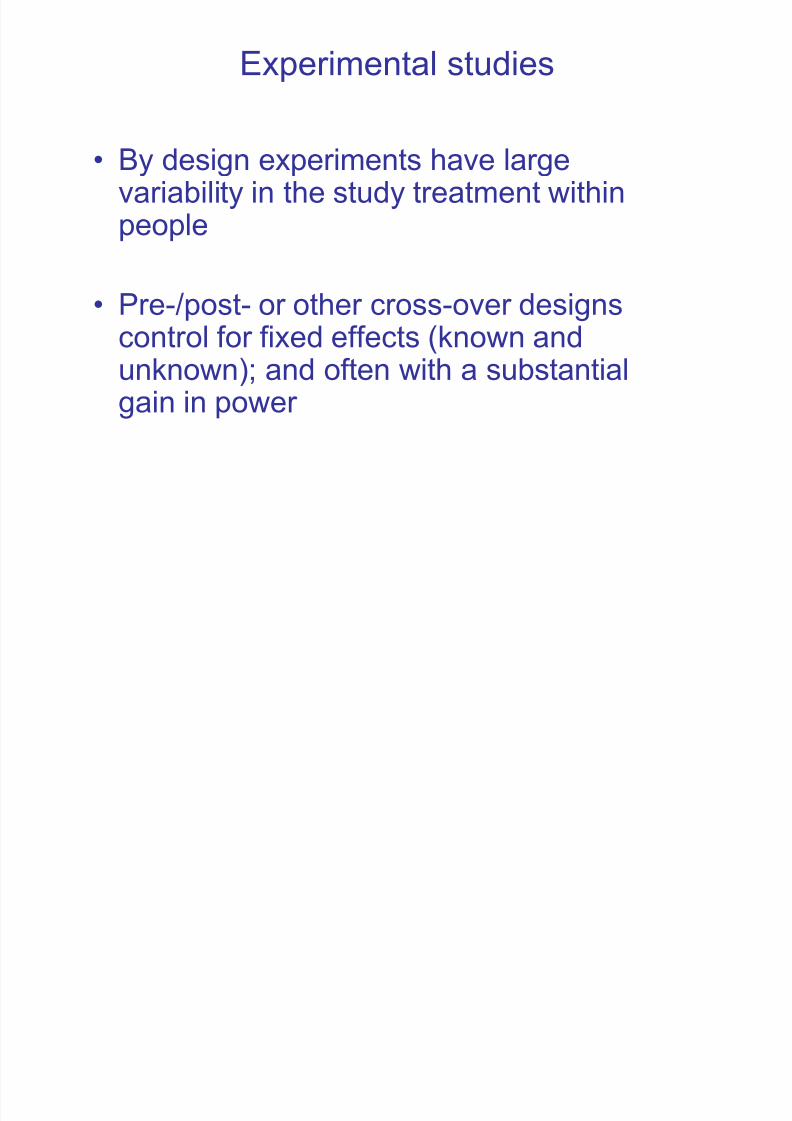
Experimental studies

• By design experiments have largevariability in the study treatment within

people

• Pre-/post- or other cross-over designscontrol for fixed effects (known andunknown); and often with a substantialgain in power



Non-experimental studies

• In non-experimental studies variability

within people over time is often not large

• With fixed effects models you control bias

from fixed effects, but often with a loss of

power



Maximal power

• Large variability in study exposure withinpeople over time

• Large variability in the study outcomebetween people over time



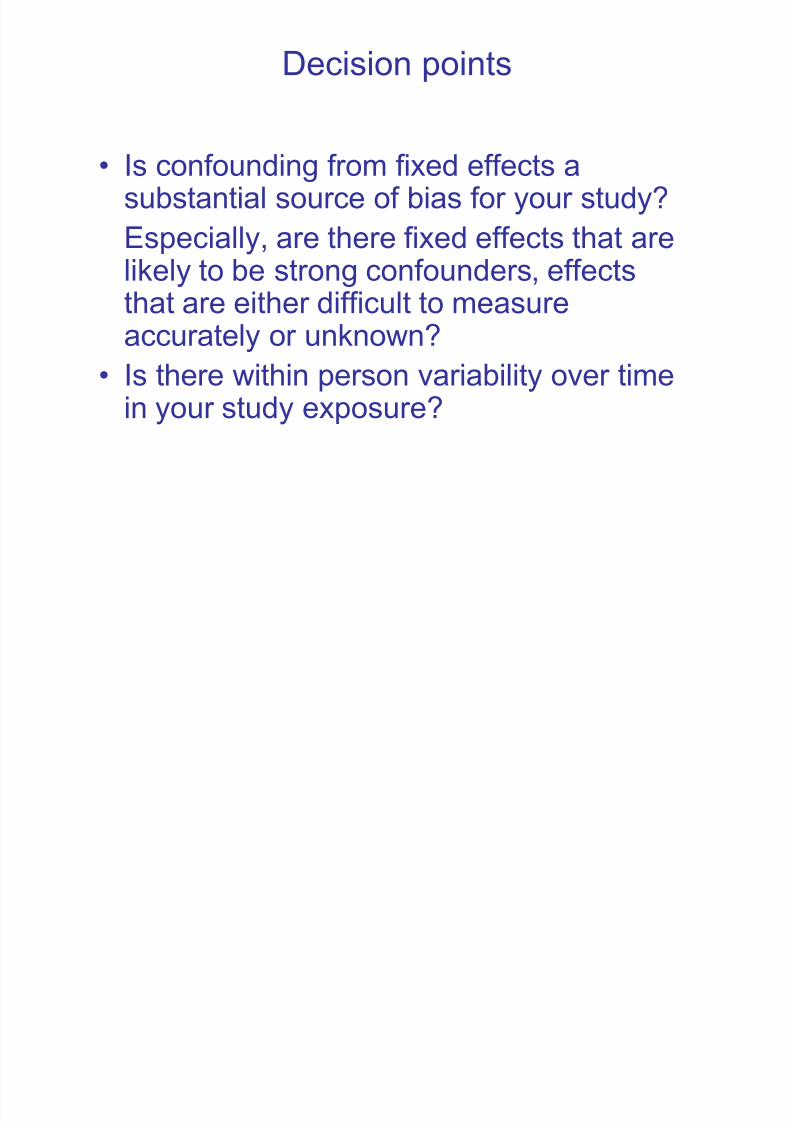
Decision points

• Is confounding from fixed effects asubstantial source of bias for your study?

Especially, are there fixed effects that arelikely to be strong confounders, effectsthat are either difficult to measureaccurately or unknown?

• Is there within person variability over timein your study exposure?



Normally distributed outcomes

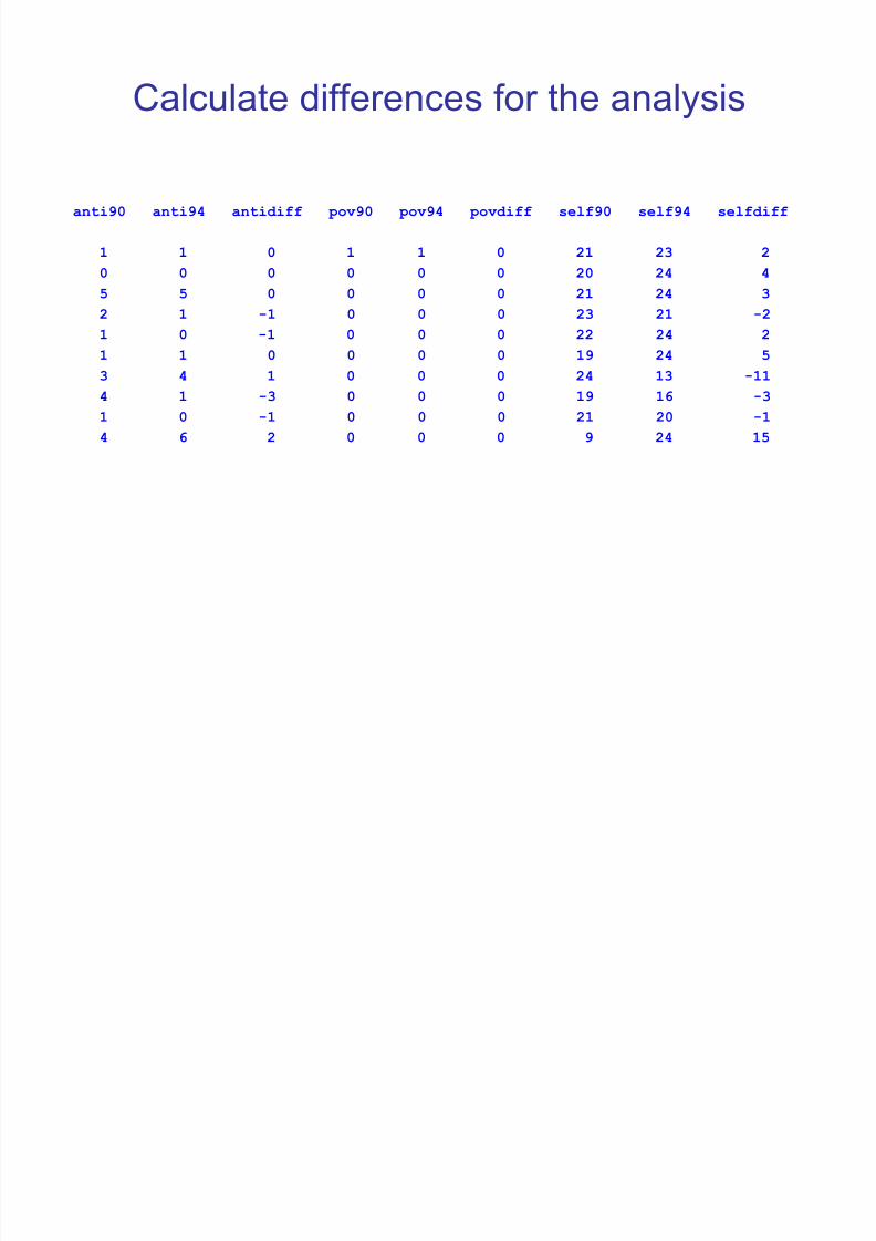
• Data: National Longitudinal Study of Youth

• Outcome: antisocial behavior (anti)• Time-varying predictors: poverty (pov) and

self-esteem (scale from 6-24))



Calculate differences for the analysis

anti90 anti94 antidiff pov90 pov94 povdiff self90 self94 selfdiff

1 1 0 1 1 0 21 23 2

0 0 0 0 0 0 20 24 4

5 5 0 0 0 0 21 24 3

2 1 -1 0 0 0 23 21 -2

1 0 -1 0 0 0 22 24 2

1 1 0 0 0 0 19 24 5

3 4 1 0 0 0 24 13 -11

4 1 -3 0 0 0 19 16 -31 0 -1 0 0 0 21 20 -1

4 6 2 0 0 0 9 24 15



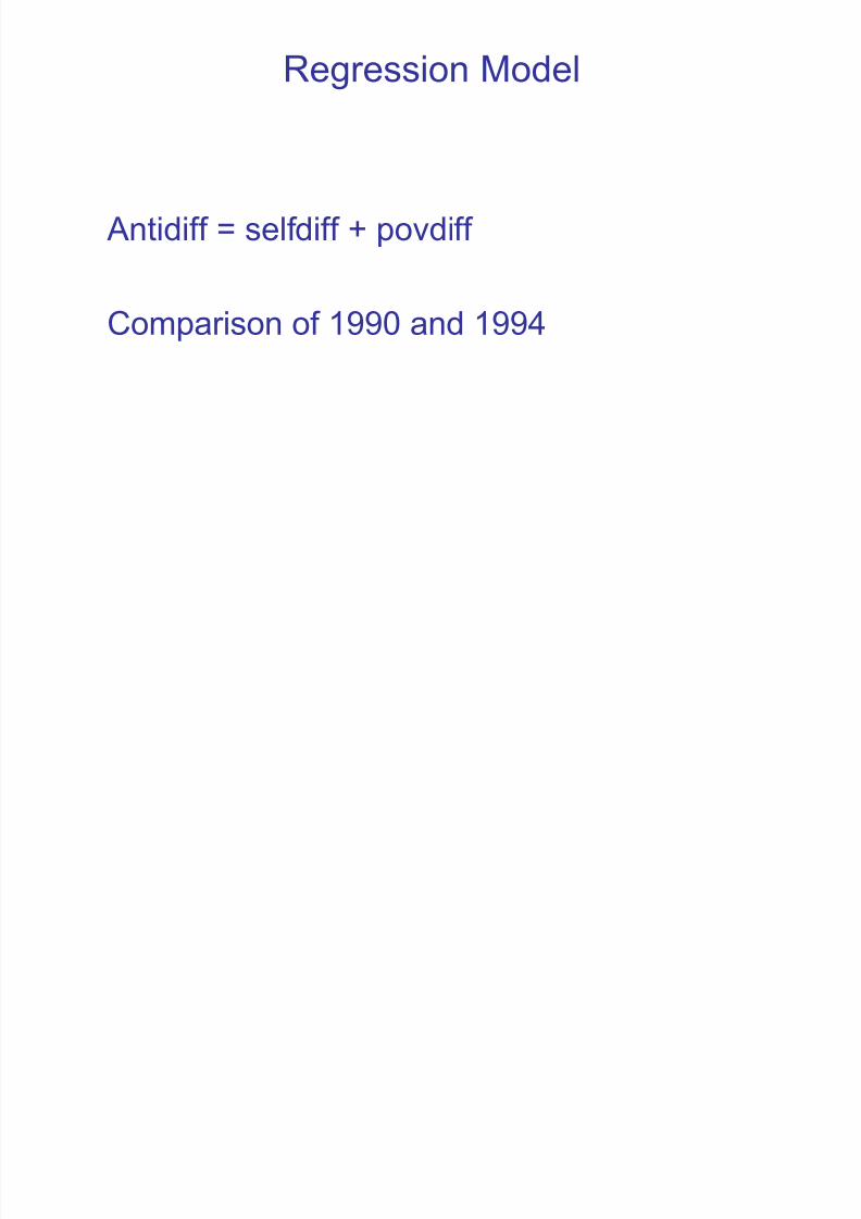
Regression Model

Antidiff = selfdiff + povdiff

Comparison of 1990 and 1994



Model using differences between

1990 and 1994

Parameter Estimates

Parameter Standard

Variable DF Estimate Error t Value Pr > |t|

Intercept 1 0.20923 0.06305 3.32 0.0010

selfdiff 1 -0.05615 0.01531 -3.67 0.0003

povdiff 1 -0.03631 0.12827 -0.28 0.7772

• Antisocial behavior decreased with higher self-esteem,

but was not significantly associated with poverty

• Both self-esteem and poverty varied across time within

people



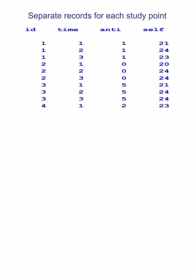
What if you have more than two

time points?

• Create separate records for each time

point and adjust for study id

• Or, create separate records and subtract

the mean value across time from the

predictors on the records



Separate records for each study point

id time anti self

1 1 1 21

1 2 1 24

1 3 1 232 1 0 20

2 2 0 24

2 3 0 24

3 1 5 21

3 2 5 24

3 3 5 24

4 1 2 23



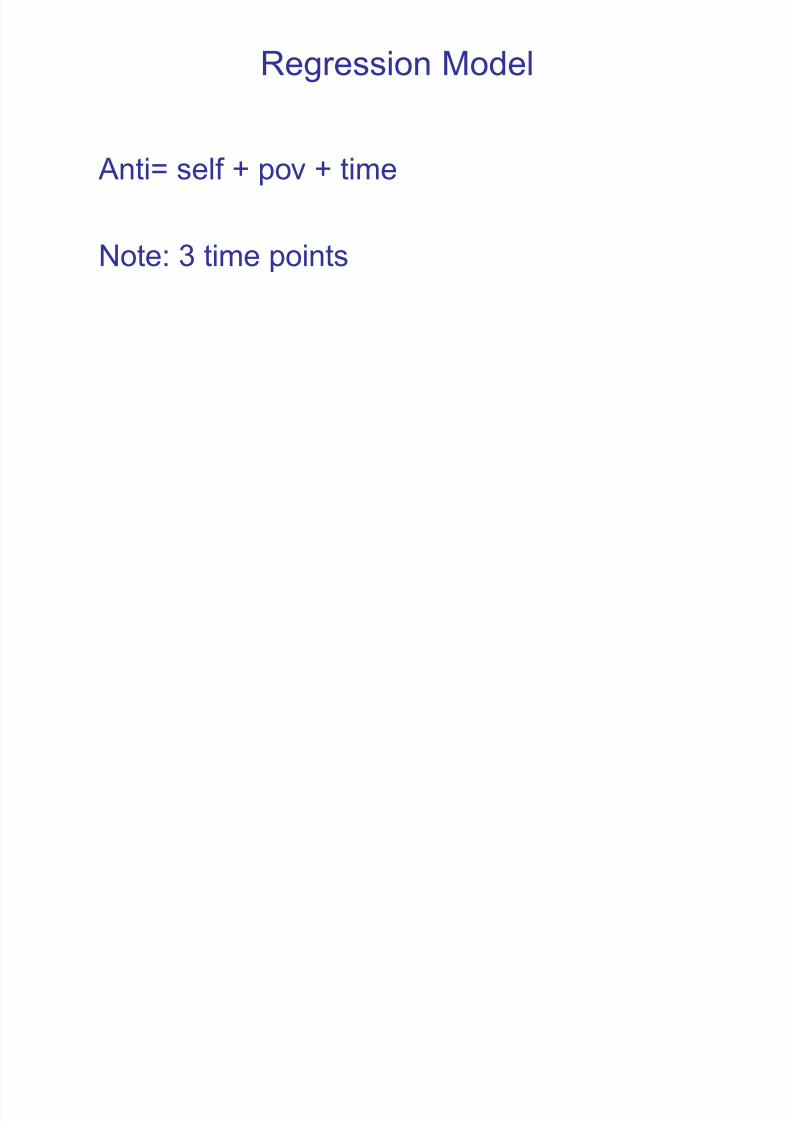
Regression Model

Anti= self + pov + time

Note: 3 time points



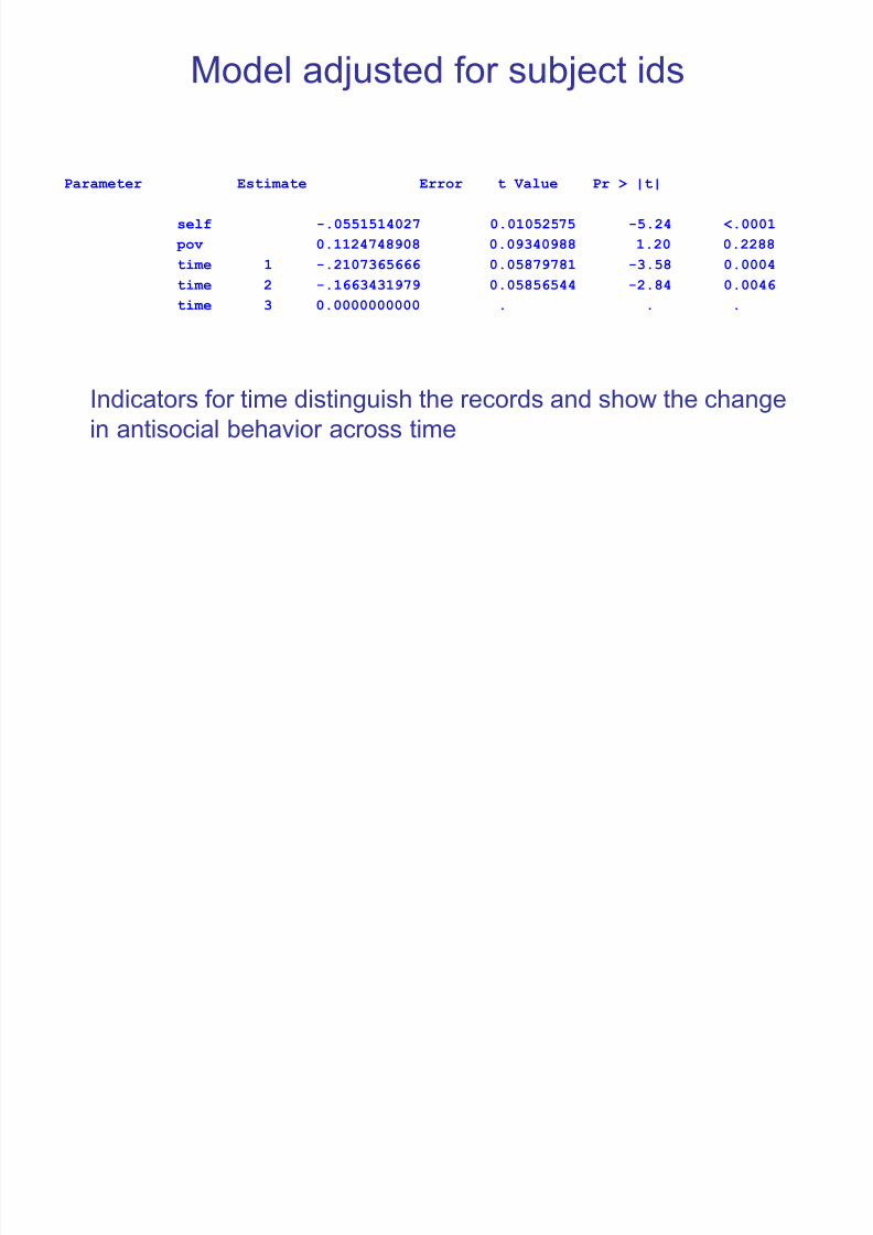
Model adjusted for subject ids

Parameter Estimate Error t Value Pr > |t|

self -.0551514027 0.01052575 -5.24 <.0001

pov 0.1124748908 0.09340988 1.20 0.2288

time 1 -.2107365666 0.05879781 -3.58 0.0004time 2 -.1663431979 0.05856544 -2.84 0.0046

time 3 0.0000000000 . . .

Indicators for time distinguish the records and show the changein antisocial behavior across time



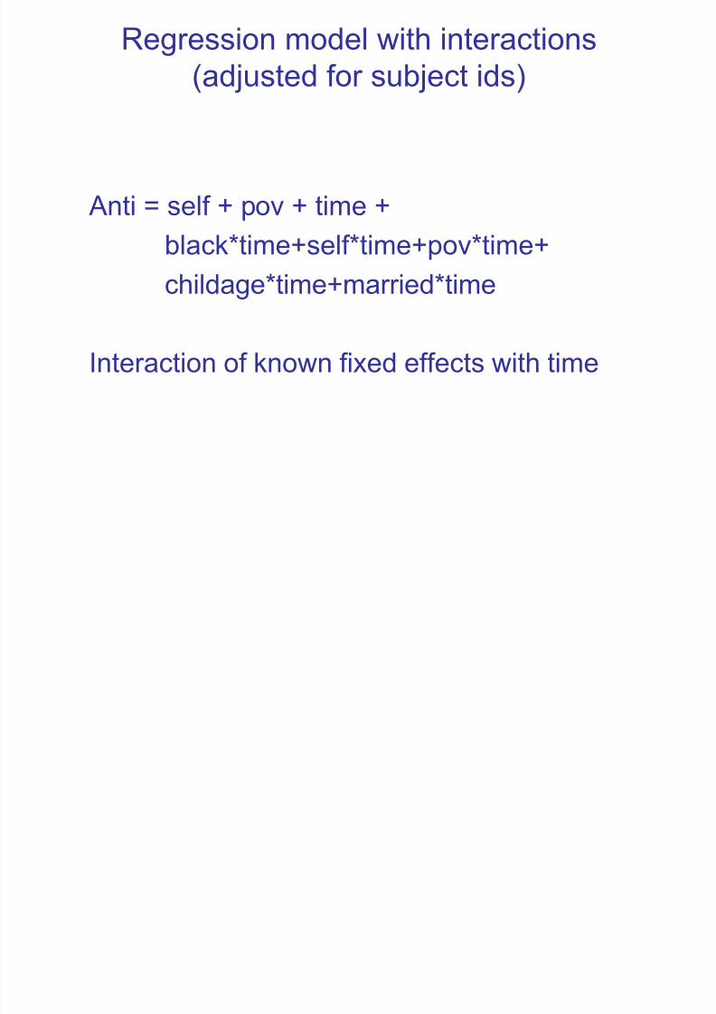
Regression model with interactions

(adjusted for subject ids)

Anti = self + pov + time +black*time+self*time+pov*time+

childage*time+married*time

Interaction of known fixed effects with time



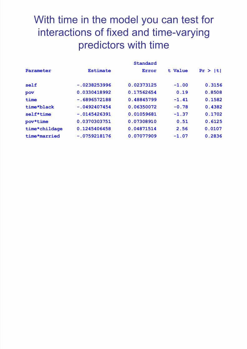
With time in the model you can test for

interactions of fixed and time-varyingpredictors with time

Standard

Parameter Estimate Error t Value Pr > |t|

self -.0238253996 0.02373125 -1.00 0.3156

pov 0.0330418992 0.17562654 0.19 0.8508

time -.6896572188 0.48845799 -1.41 0.1582

time*black -.0492407454 0.06350072 -0.78 0.4382

self*time -.0145426391 0.01059681 -1.37 0.1702

pov*time 0.0370303751 0.07308910 0.51 0.6125

time*childage 0.1245406458 0.04871514 2.56 0.0107

time*married -.0759218176 0.07077909 -1.07 0.2836



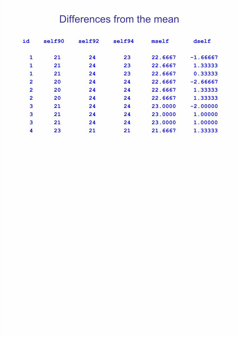
Differences from the mean

id self90 self92 self94 mself dself

1 21 24 23 22.6667 -1.66667

1 21 24 23 22.6667 1.33333

1 21 24 23 22.6667 0.333332 20 24 24 22.6667 -2.66667

2 20 24 24 22.6667 1.33333

2 20 24 24 22.6667 1.33333

3 21 24 24 23.0000 -2.000003 21 24 24 23.0000 1.00000

3 21 24 24 23.0000 1.00000

4 23 21 21 21.6667 1.33333



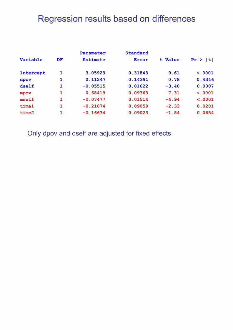
Regression Model

anti=dpov+dself+dtime+mpow+mself



Regression results based on differences

Parameter Standard

Variable DF Estimate Error t Value Pr > |t|

Intercept 1 3.05929 0.31843 9.61 <.0001

dpov 1 0.11247 0.14391 0.78 0.4346

dself 1 -0.05515 0.01622 -3.40 0.0007

mpov 1 0.68419 0.09363 7.31 <.0001

mself 1 -0.07477 0.01514 -4.94 <.0001

time1 1 -0.21074 0.09059 -2.33 0.0201time2 1 -0.16634 0.09023 -1.84 0.0654

Only dpov and dself are adjusted for fixed effects



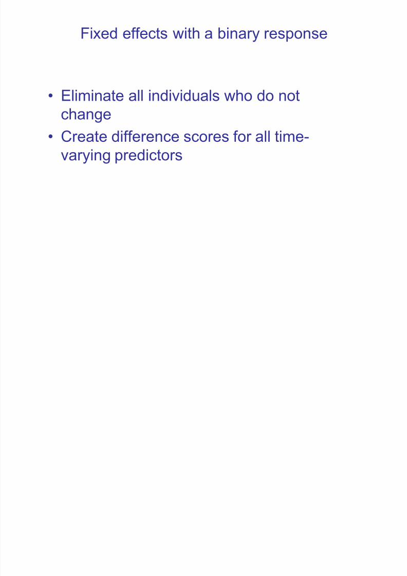
Fixed effects with a binary response

• Eliminate all individuals who do not

change

• Create difference scores for all time-

varying predictors



Teenage poverty in years 1 and 5

Table of pov1 by pov5

pov1 pov5

Frequency‚ 0‚ 1‚ Total

ƒƒƒƒƒƒƒƒƒˆƒƒƒƒƒƒƒƒˆƒƒƒƒƒƒƒƒˆ

0 ‚ 516 ‚ 234 ‚ 750

ƒƒƒƒƒƒƒƒƒˆƒƒƒƒƒƒƒƒˆƒƒƒƒƒƒƒƒˆ 1 ‚ 211 ‚ 190 ‚ 401

ƒƒƒƒƒƒƒƒƒˆƒƒƒƒƒƒƒƒˆƒƒƒƒƒƒƒƒˆ

Total 727 424 1151



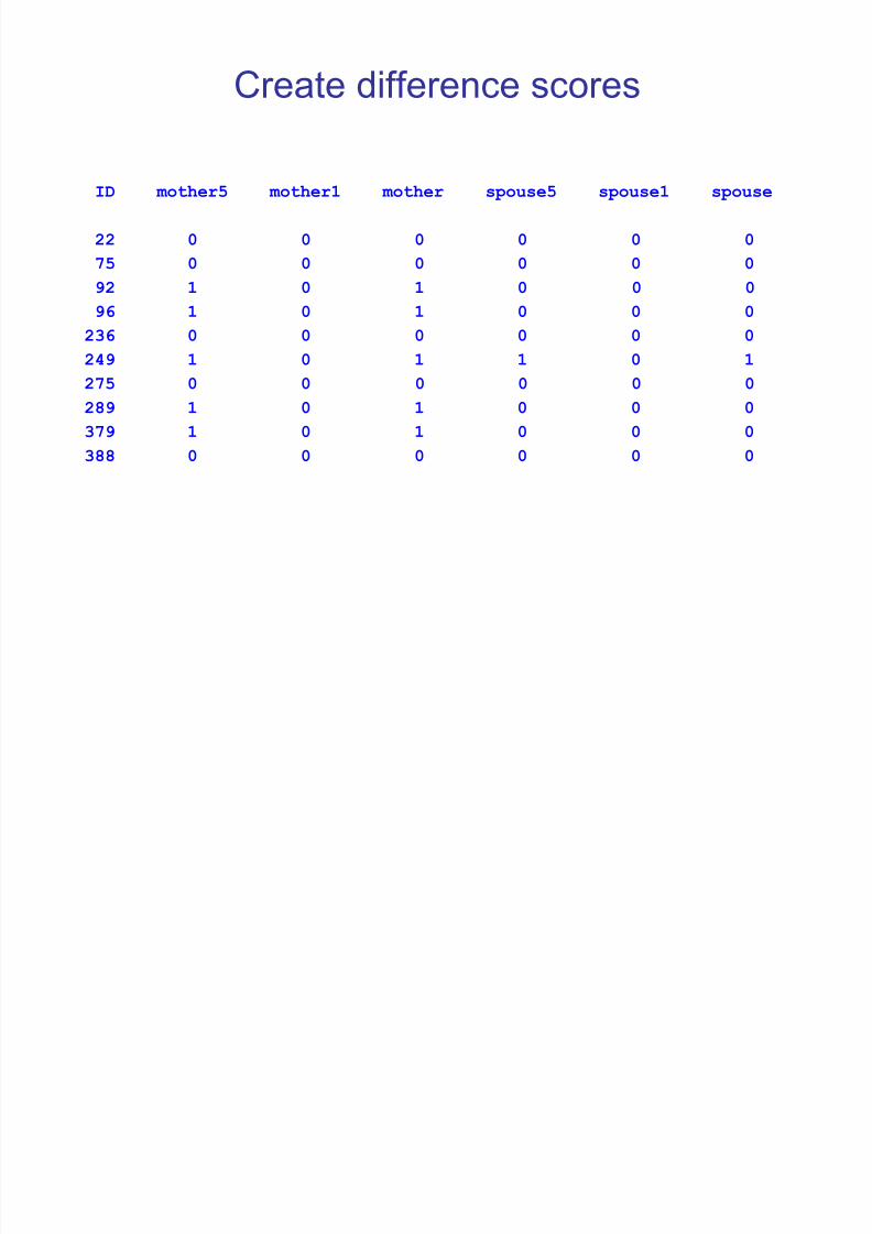
Create difference scores

ID mother5 mother1 mother spouse5 spouse1 spouse

22 0 0 0 0 0 0

75 0 0 0 0 0 092 1 0 1 0 0 0

96 1 0 1 0 0 0

236 0 0 0 0 0 0

249 1 0 1 1 0 1

275 0 0 0 0 0 0

289 1 0 1 0 0 0

379 1 0 1 0 0 0

388 0 0 0 0 0 0



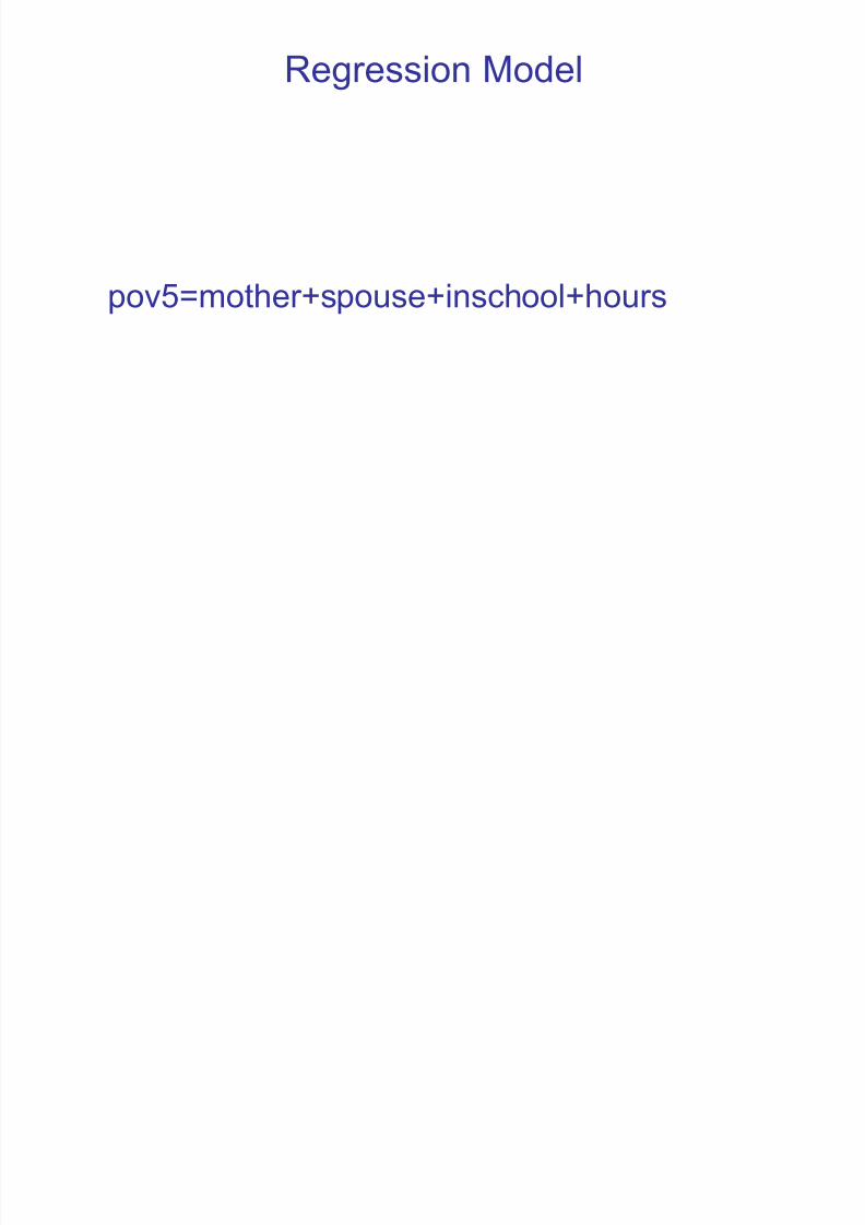
Regression Model

pov5=mother+spouse+inschool+hours



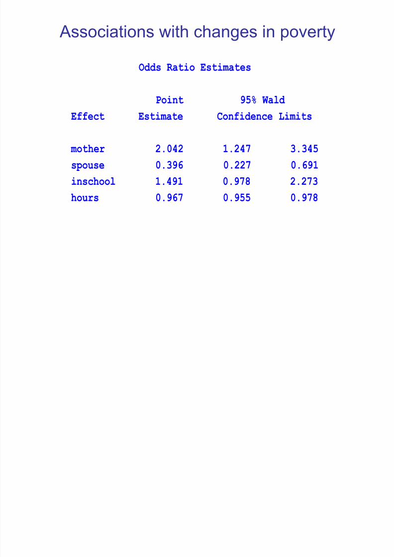
Associations with changes in poverty

Odds Ratio Estimates

Point 95% Wald

Effect Estimate Confidence Limits

mother 2.042 1.247 3.345

spouse 0.396 0.227 0.691

inschool 1.491 0.978 2.273

hours 0.967 0.955 0.978



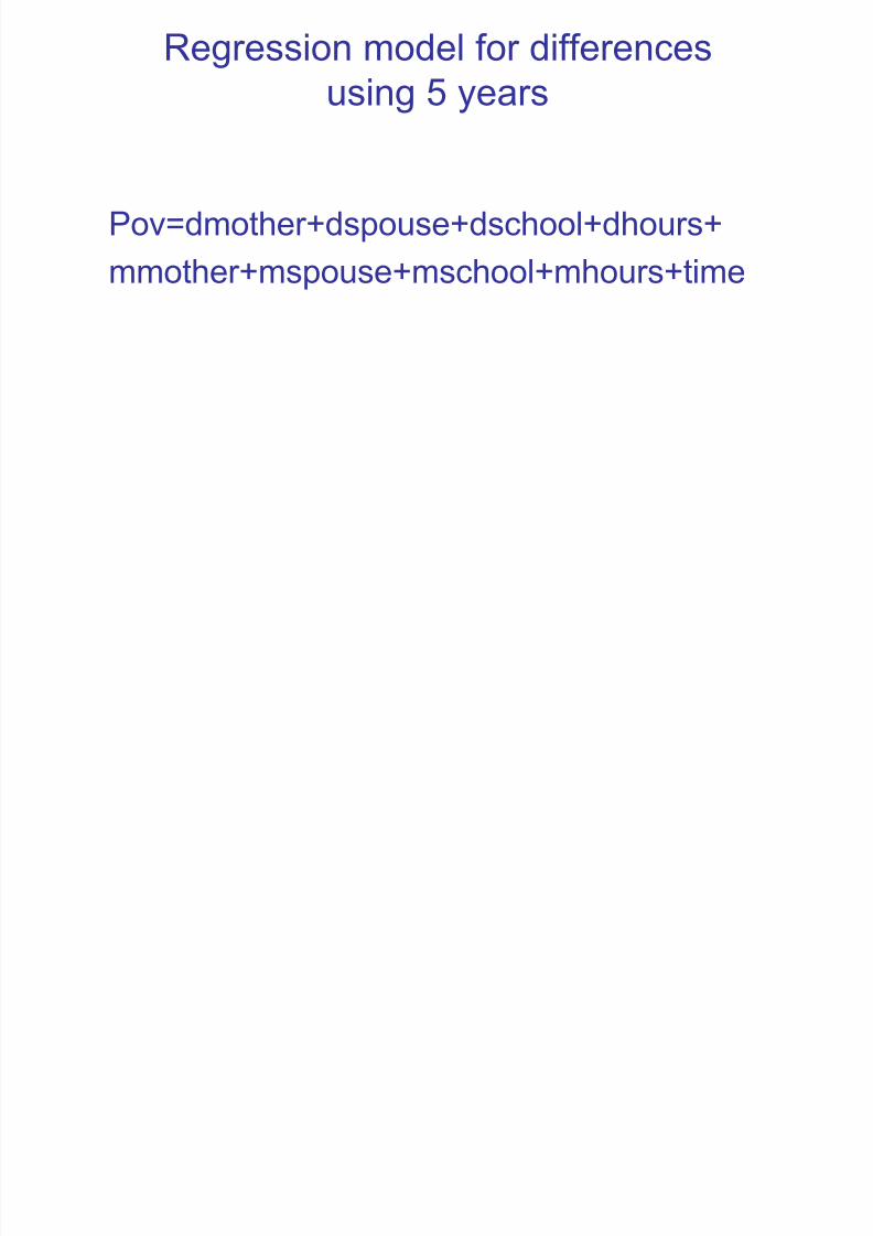
Regression model for differences

using 5 years

Pov=dmother+dspouse+dschool+dhours+

mmother+mspouse+mschool+mhours+time



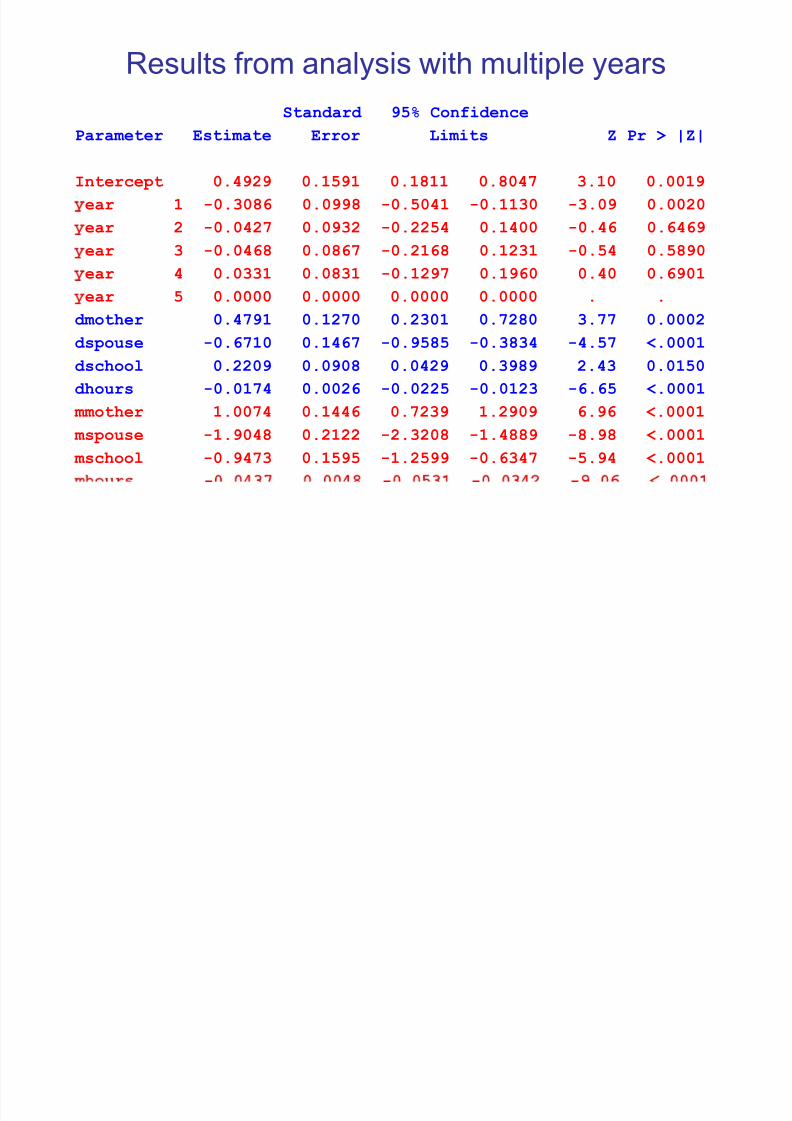
Results from analysis with multiple years

Standard 95% Confidence

Parameter Estimate Error Limits Z Pr > |Z|

Intercept 0.4929 0.1591 0.1811 0.8047 3.10 0.0019

ear 1 -0.3086 0.0998 -0.5041 -0.1130 -3.09 0.0020

ear 2 -0.0427 0.0932 -0.2254 0.1400 -0.46 0.6469

ear 3 -0.0468 0.0867 -0.2168 0.1231 -0.54 0.5890

ear 4 0.0331 0.0831 -0.1297 0.1960 0.40 0.6901

ear 5 0.0000 0.0000 0.0000 0.0000 . .

dmother 0.4791 0.1270 0.2301 0.7280 3.77 0.0002

dspouse -0.6710 0.1467 -0.9585 -0.3834 -4.57 <.0001

dschool 0.2209 0.0908 0.0429 0.3989 2.43 0.0150

dhours -0.0174 0.0026 -0.0225 -0.0123 -6.65 <.0001

mmother 1.0074 0.1446 0.7239 1.2909 6.96 <.0001

mspouse -1.9048 0.2122 -2.3208 -1.4889 -8.98 <.0001

mschool -0.9473 0.1595 -1.2599 -0.6347 -5.94 <.0001

- - - -



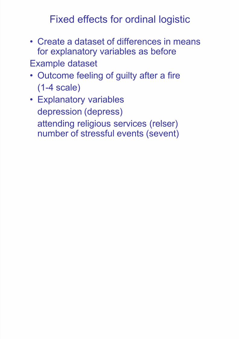
Fixed effects for ordinal logistic

• Create a dataset of differences in meansfor explanatory variables as before

Example dataset

• Outcome feeling of guilty after a fire(1-4 scale)

• Explanatory variables

depression (depress)

attending religious services (relser)number of stressful events (sevent)



Results from proportional odds model



Intercept1 2.1085 0.3422 1.4378 2.7791 6.16 <.0001

Intercept2 2.9643 0.3492 2.2799 3.6487 8.49 <.0001

Intercept3 3.7853 0.3653 3.0693 4.5012 10.36 <.0001

ddepress -0.3001 0.1389 -0.5724 -0.0278 -2.16 0.0308

drelser -0.1462 0.1600 -0.4598 0.1673 -0.91 0.3606

dsevent -0.1728 0.0798 -0.3292 -0.0165 -2.17 0.0303

mdepress -0.7831 0.1258 -1.0298 -0.5365 -6.22 <.0001

mrelser 0.3619 0.1572 0.0538 0.6700 2.30 0.0213 msevent -0.0579 0.1294 -0.3116 0.1957 -0.45 0.6543

time 1 -0.7816 0.1712 -1.1172 -0.4460 -4.56 <.0001

time 2 -0.4850 0.1696 -0.8175 -0.1526 -2.86 0.0042

time 3 0.0000 0.0000 0.0000 0.0000 . .



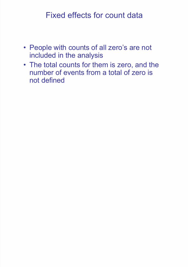
Fixed effects for count data

• People with counts of all zero‟s are not

included in the analysis• The total counts for them is zero, and the

number of events from a total of zero isnot defined



Pre- / post-comparison

Subtract the pre- counts from the post-

counts

• You can test if the difference is zero

• You can include time varying predictors



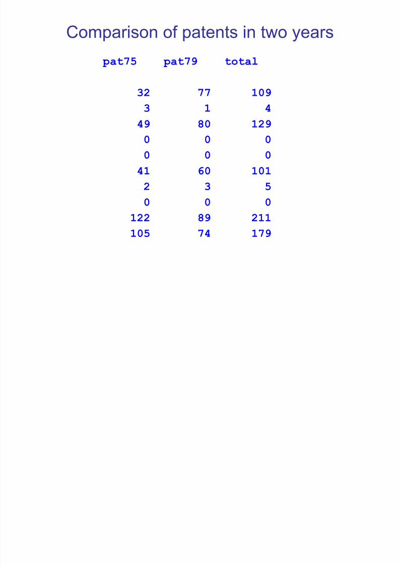
Comparison of patents in two years

at75 pat79 total

32 77 109

3 1 4

49 80 1290 0 0

0 0 0

41 60 101

2 3 5

0 0 0

122 89 211

105 74 179



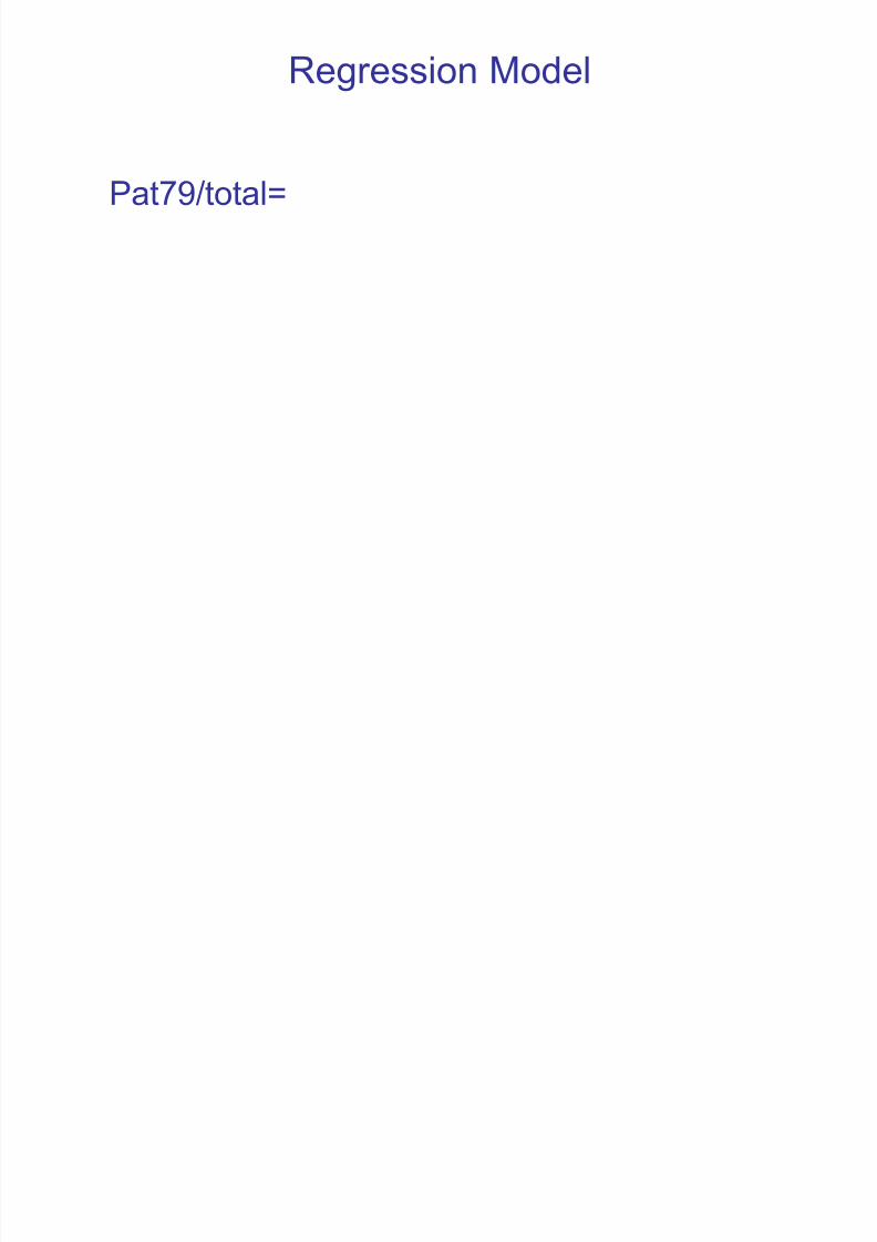
Regression Model

Pat79/total=



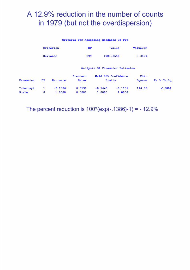
A 12.9% reduction in the number of counts

in 1979 (but not the overdispersion)

Criteria For Assessing Goodness Of Fit

Criterion DF Value Value/DF

Deviance 299 1001.3656 3.3490

Analysis Of Parameter Estimates

Standard Wald 95% Confidence Chi-

Parameter DF Estimate Error Limits Square Pr > ChiSq

Intercept 1 -0.1386 0.0130 -0.1640 -0.1131 114.03 <.0001

Scale 0 1.0000 0.0000 1.0000 1.0000

The percent reduction is 100*(exp(-.1386)-1) = - 12.9%



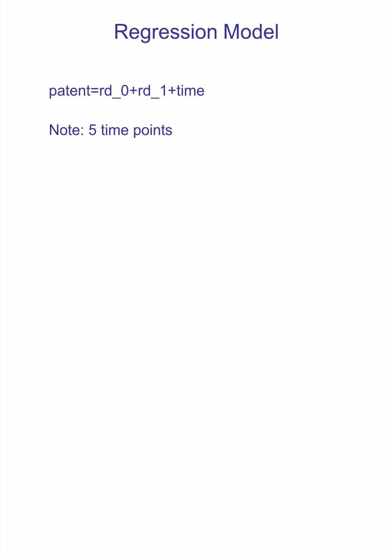
Regression Model

patent=rd_0+rd_1+time

Note: 5 time points



More than two measurements

For the explanatory variables subtract the meanfor all years from each year‟s value

(rd_0 and rd_1 are expenditures in yrs 0 and 1

id t drd_0 rd_0 mrd_0 drd_1 rd_1 mrd_1

1 1 -0.09473 0.92327 1.01800 0.02046 1.02901 1.00855

1 2 0.00509 1.02309 1.01800 -0.08528 0.92327 1.00855

1 3 -0.04560 0.97240 1.01800 0.01454 1.02309 1.00855

1 4 0.07700 1.09500 1.01800 -0.03615 0.97240 1.008551 5 0.05824 1.07624 1.01800 0.08645 1.09500 1.00855

2 1 -0.58923 -1.48519 -0.89596 0.22642 -0.68464 -0.91106

2 2 -0.29899 -1.19495 -0.89596 -0.57413 -1.48519 -0.91106

2 3 0.28628 -0.60968 -0.89596 -0.28389 -1.19495 -0.91106

2 4 0.31514 -0.58082 -0.89596 0.30138 -0.60968 -0.91106

2 5 0.28681 -0.60915 -0.89596 0.33024 -0.58082 -0.91106



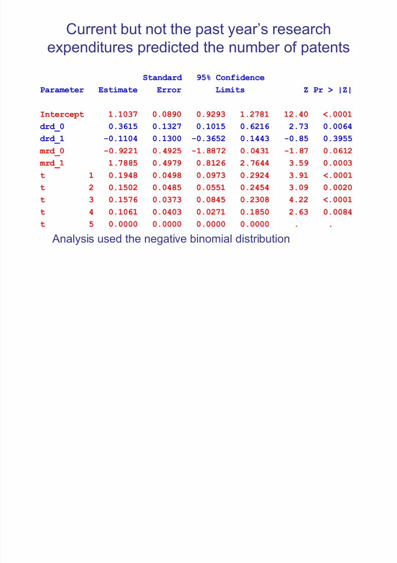
Current but not the past year‟s research

expenditures predicted the number of patents



Intercept 1.1037 0.0890 0.9293 1.2781 12.40 <.0001

drd_0 0.3615 0.1327 0.1015 0.6216 2.73 0.0064

drd_1 -0.1104 0.1300 -0.3652 0.1443 -0.85 0.3955

mrd_0 -0.9221 0.4925 -1.8872 0.0431 -1.87 0.0612

mrd_1 1.7885 0.4979 0.8126 2.7644 3.59 0.0003

t 1 0.1948 0.0498 0.0973 0.2924 3.91 <.0001

t 2 0.1502 0.0485 0.0551 0.2454 3.09 0.0020

t 3 0.1576 0.0373 0.0845 0.2308 4.22 <.0001

t 4 0.1061 0.0403 0.0271 0.1850 2.63 0.0084

t 5 0.0000 0.0000 0.0000 0.0000 . . Analysis used the negative binomial distribution



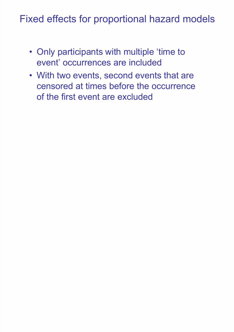
Fixed effects for proportional hazard models

• Only participants with multiple „time to

event‟ occurrences are included

• With two events, second events that arecensored at times before the occurrence

of the first event are excluded



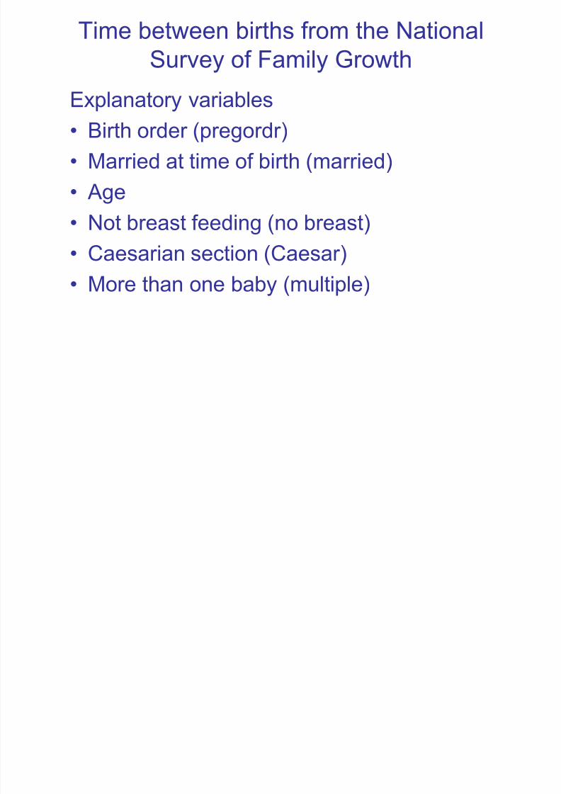
Time between births from the National

Survey of Family Growth

Explanatory variables

• Birth order (pregordr)

• Married at time of birth (married)• Age

• Not breast feeding (no breast)

• Caesarian section (Caesar)• More than one baby (multiple)



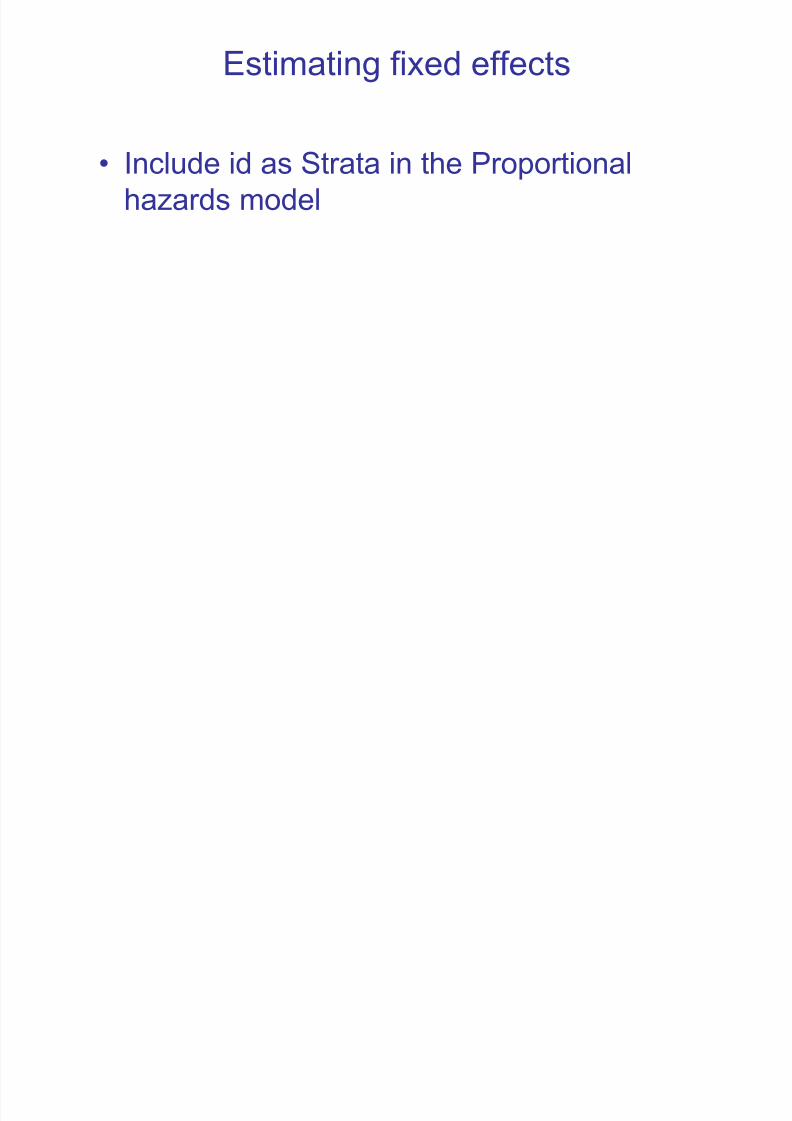
Estimating fixed effects

• Include id as Strata in the Proportional

hazards model



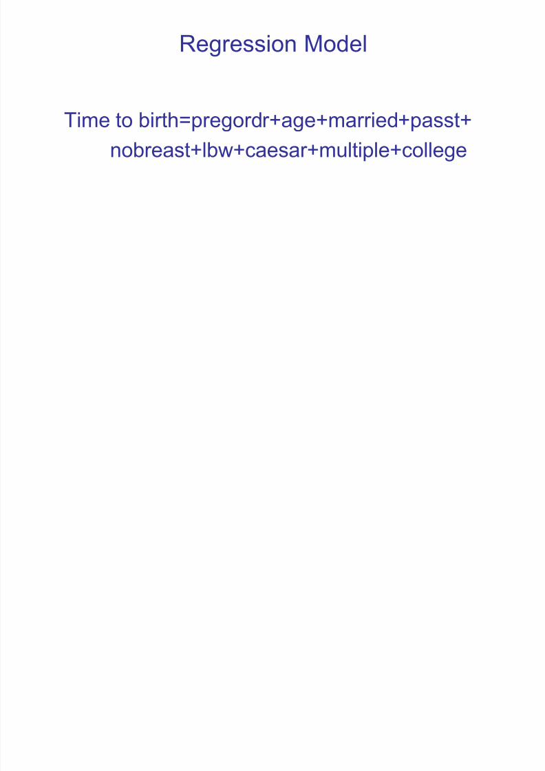
Regression Model

Time to birth=pregordr+age+married+passt+

nobreast+lbw+caesar+multiple+college



Proportional hazard results

Analysis of Maximum Likelihood Estimates

Parameter Standard Hazard

Variable DF Estimate Error Chi-Square Pr > ChiSq Ratio

pregordr 1 -0.71663 0.03372 451.7316 <.0001 0.488age 1 0.0000818 0.0001125 0.5285 0.4672 1.000

married 1 0.18307 0.06958 6.9219 0.0085 1.201

passt 1 0.07590 0.06863 1.2229 0.2688 1.079

nobreast 1 -0.12832 0.06047 4.5035 0.0338 0.880

lbw 1 -0.23642 0.08117 8.4832 0.0036 0.789

caesar 1 -0.07839 0.09272 0.7148 0.3979 0.925

multiple 1 -0.60731 0.21852 7.7240 0.0054 0.545college 0 0 . . . .

Note: College education is a fixed effect and not estimable



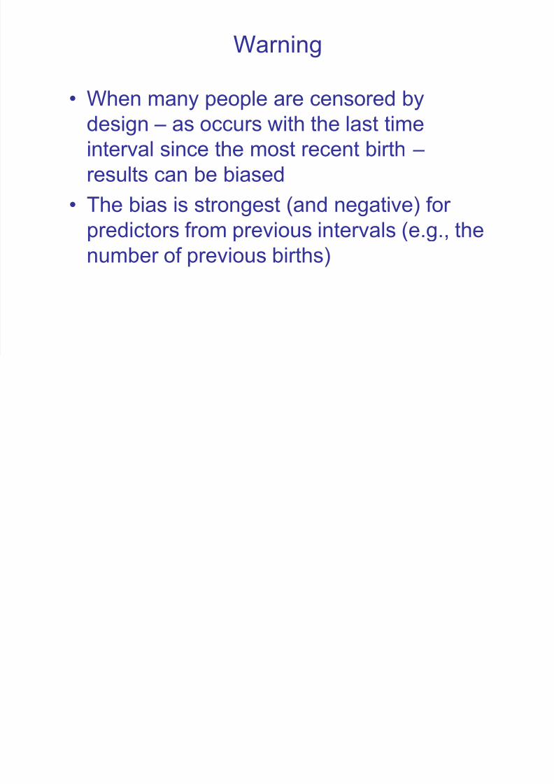
Warning

• When many people are censored by

design – as occurs with the last time

interval since the most recent birth –

results can be biased

• The bias is strongest (and negative) for

predictors from previous intervals (e.g., the

number of previous births)

Fixed Effects Regression

Documents

Transcript of Fixed Effects Regression