Fitting Subdivision Surfaces to Unorganized Point Data Using SDM

Kin-Shing D. Cheng† Wenping Wang† Hong Qin‡ Kwan-Yee K. Wong† Huaiping Yang† Yang Liu†

† Department of Computer Science

The University of Hong Kong

Pokfulam Road, Hong Kong, China

{ksdcheng, wenping}@cs.hku.hk

‡ Department of Computer Science

State University of New York at Stony Brook

Stony Brook, New York, U.S.A.

qin@cs.sunysb.edu

Abstract

We study the reconstruction of smooth surfaces frompoint clouds. We use a new squared distance error term inoptimization to fit a subdivision surface to a set of unorga-nized points, which defines a closed target surface of arbi-trary topology. The resulting method is based on the frame-work of squared distance minimization (SDM) proposed byPottmann et al. Specifically, with an initial subdivision sur-face having a coarse control mesh as input, we adjust thecontrol points by optimizing an objective function throughiterative minimization of a quadratic approximant of thesquared distance function of the target shape. Our exper-iments show that the new method (SDM) converges muchfaster than the commonly used optimization method usingthe point distance error function, which is known to haveonly linear convergence. This observation is further sup-ported by our recent result that SDM can be derived fromthe Newton method with necessary modifications to makethe Hessian positive definite and the fact that the Newtonmethod has quadratic convergence.

1. Introduction

1.1. Problem Statement

We propose a method that fits a Loop’s subdivision sur-faceS [22] to a target surfaceΓ defined by a set of unor-ganized points. The availability of the connectivity infor-mation of the target points is not assumed. Although weuse Loop’s surface, the basic framework can be applied toother linear subdivision schemes as well. We iteratively up-date the subdivision surfaceS to make it converge to a tar-get shape by optimizing an objective error function. Previ-ous subdivision surface fitting methods use the distance be-tween a point on the fitting surface and the correspondingfoot point on the target surface for minimizing the objective

function; we will call these methodspoint distance mini-mization, or PDM. We use a quadratic approximant of thesquared distance (SD) error function proposed by Pottmannet al [33], and show that the SD error function leads to betterfitting results than using the conventional point distance er-ror function. Our method will be called SDM, standing forsquared distance minimization.

Although the Gauss-Newton method is preferred forsolving a general nonlinear least squares problem, PDMis still the predominant optimization method used for sur-face fitting in CAD and graphics. By proving that SDMcan be derived directly from the Newton method, we showthat SDM is a more refined optimization technique than theGauss-Newton method, which omits the true Hessian of anobjective function. The purpose of this paper is to demon-strate that SDM is indeed a superior optimization techniquefor fitting a subdivision surface than the commonly usedPDM.

1.2. Related Work

The problem of computing a compact surface repre-sentation of a target shape given by a set of unorganizeddata points has many applications in computer graphics,CAD, and computer vision. A typical formulation of theproblem is computing a piecewise smooth surface, whichcan be a B-spline surface (including a NURBS surface)or a subdivision surface, that approximates a given tar-get shape within a pre-specified error tolerance. Comparedwith the traditional methods based on B-spline surfaces,the approach using subdivision surfaces has gained in-creasing attention due to its ability to deal with generalobject topology as well as arbitrary connectivity of thecontrol mesh [45, 46]. Approaches of different categorieswere proposed over the past decade. These include lo-cal fitting approaches [10–12, 25–27, 29, 38], active surfaceapproaches [4, 6, 7, 18, 20, 24, 28, 34, 40, 41, 43, 44], im-plicit surface approaches [1,2,30,39] and other approaches

[13,14,16,17,21].Among the previous work, some are more relevant to our

approach. In Hoppe et al’s method [11,12], an initial densemesh is generated from a set of unorganized points and isthen decimated to fit the target shape via optimization of anenergy function. Finally, a smooth subdivision surface is ob-tained from the mesh again via optimization. In Ma et al’smethod [25–27], base surfaces are built for obtaining the pa-rameter values of the data points. Then a least squares pro-cedure is used to fit B-spline surfaces on general quadrilat-eral topology and Catmull-Clark surfaces on extraordinarycorner patches. In [29], closest point search on Loop’s sur-face is performed by combining Newton iteration and non-linear minimization, followed by an optimization with re-spect to theL2 metric. In these methods, when the geo-metric error between the fitting surface and the target shapeneeds to be measured or minimized, the error function is de-fined by the summation of the squared distance between apoint on the fitting surface and its closest point on the targetshape. Hence, these methods use PDM (point distance mini-mization). Such optimization schemes, also called the alter-nating methods [35], are typically used for solving separa-ble nonlinear least squares problems, and are known to haveonly linear convergence. In this paper, we propose to replacethe conventionally-used geometric error with the SD errorfunction. The resulting method, called SDM (squared dis-tance minimization), can be applied to any existing frame-works in which distance functions are used to define a goalfunction.

2. Preliminaries

2.1. SDM

Pottmann et al. [31–33] proposed a general paradigm ofshape approximation based on the minimization of a novelquadratic approximant of the squared distance function. Letp denote the foot point on the target surfaceΓ of a sam-ple pointv0 from a fitting surface, i.e.p is the closest pointon Γ to v0. Let d = ‖v0 − p‖2. Let ρ1 andρ2 be the prin-cipal curvature radii of the surfaceΓ atp. Let T1 andT2 bethe unit vectors in the corresponding principal curvature di-rections. LetN be the unit normal vector, i.e.N = T1×T2.A quadratic appproximant of the squared distance functionfrom a variable pointv in the neighborhood ofv0 to Γ isgiven by

F+d (v) =

d

d + |ρ1|[(v − p)T1]

2 (1)

+d

d + |ρ2|[(v − p)T2]

2 + [(v − p)N ]2

This formula is called the squared distance (SD) error func-tion. Pottmann et al. applied SDM successfully to solve a

series of geometric optimization problems, including theproblem of fitting B-spline curves and surfaces to somesmooth target shapes [32, 33]. Yang et al. [42] studied howto define initial shapes and adjust the number of controlpoints when using the SDM for B-spline curve approxima-tion. The ellipsoid in Figure 1 shows an iso-distance surfacedefined by the SD error function for surface fitting.

Figure 1. An iso-surface of the SD error func-tion, with a local coordinate frame at the pointp.

For comparison, the (squared) point distance (PD) errorfunction is defined by

F+(v) = ‖v − p‖22. (2)

Accordingly, optimization schemes using the PD error func-tion will be called PDM. Intuitively, unlike the PD errorfunction, the SD error function takes the local geometry ofthe target surfaceΓ into account. In fact, SDM is a New-ton method with proper modification of possibly indefiniteHessian; the proof of this fact is given in the technical re-port [5]. Hence, we expect better convergence behavior us-ing SDM than using PDM, which is known to have only lin-ear convergence.

2.2. Loop’s Surface

Loop [22] proposed a subdivision scheme for triangu-lated control polyhedra. For one level of subdivision, a tri-angle is split into four triangles by adding on each edge anew vertexX given by

X =3

8(Xa + Xb) +

1

8(Xc + Xd),

whereXa, Xb are the two vertices of the edge, andXc, Xd

are the other vertices of the two triangles that are incidenttothe edgeXaXb. Then the original vertices are modified by

the following rule:

X = (1 − kβ)X + β

k∑

i=1

Xi,

wherek is the degree of the vertexX andXi’s are the neigh-boring points ofX, β = 3/16 if k = 3, and

β =1

k

[

5

8−

(

3

8+

1

4cos2

(

2π

k

))2]

if k > 3.

3. Main Steps

Our SDM method has the following steps:

1. Normalization of the target shape:The target shape is normalized by scaling so that alldata points fall in the cube[0, 1]3. This is to make thevalues of the energy terms unit-less.

2. Pre-computation of distance and curvature:To quickly compute foot points for setting up errorfunctions, the distance field of the target surfaceΓ andcurvatures ofΓ at all data points are computed in a pre-processing step.

3. Initial mesh specification:To obtain an initial control mesh, we build an octree forthe target shape and then generate the initial mesh fromthe octree cells using the Marching Cubes method [23].See Section 4.3.

4. Sampling points on the fitting surface:A set of sample points are generated on the limit sur-face for setting up the error functions and error evalu-ation. These sample points are generated using the ap-proach devised by Stam [36,37].

5. Optimization:Let vk,0, k = 1, 2, . . . , N , be sample points on the fit-ting subdivision surface. Letpk be the foot point onΓof the sample pointvk,0. Denotedk = ‖vk,0 − pk‖2.Let ρk,1 andρk,2 be the principal curvature radii ofΓat pk. Let vk be a variable point in the neighborhoodof vk,0. We callvk a variable sample point associatedwith vk0. Then the SDM error function is defined as

F+ =1

N

N∑

k=1

F+dk

(vk) + λFs,

and

F+dk

(vk) =dk

dk + |ρk,1|[(vk − pk)Tk1]

2

+dk

dk + |ρk,2|[(vk − pk)Tk2]

2

+ [(vk − pk)Nk]2,

whereF+dk

(·) is the quadratic approximation for thesquared distance function from a variable point,Tk1

andTk2 are the unit vectors of the principal curvaturedirections,Nk is the unit normal vector ofΓ at pk, Fs

is a smoothing term andλ is a constant.Since the variable sample pointvk is a linear com-

bination of the control pointsPi, the functionF+ isa quadratic function of thePi. Thus the updated con-trol pointsPi can be computed by solving a linear sys-tem of equations. Since each variable sample pointvk

is only influenced by a small number of control points,the matrix for the resulting linear system of equationsis sparse. We use a conjugate gradient (CG) methodthat exploits the sparsity of the coefficient matrix tosolve the linear system of equations. The conjugategradient solver is terminated if the relative error im-provement is less than10−7 or the number of itera-tions reaches 200.

6. Fitting error evaluation:After the control points have been updated, the maxi-mum and average fitting errors are evaluated. The max-imum approximation errorEm is defined by the max-imum of the distances of all the sample pointsvk,0 onthe fitting surfaceS to the target shapeΓ, i.e.

Em = maxk

{||pk − vk,0||2}.

The average errorEa, i.e. l2 error , is defined as

Ea =

[

1

N

∑

k

||pk − vk,0||22

]1

2

.

7 Refinement and termination: The fitting process isstopped if a pre-specified error threshold is satis-fied. Otherwise, we repeat steps 4 to 6 until the resultis satisfactory. Whenever the fitting error stops get-ting improved and stays above the error threshold,new control points are inserted in regions of large er-rors to provide greater degree of freedom for betterfitting.

4. Implementation Issues

4.1. Curvature Pre-computation

The curvature information of the target shape can bepre-computed and stored for later use. There are existingmethods, such as [9], for estimating curvatures from pointclouds. We employ the following simple method for ourpurpose. For a given target pointQi, its neighboring pointsQn(i,j) are identified. In our examples, the neighborhoodsize is set to be0.075, which is chosen based on data sam-pling density of our test examples. LetOi denote the cen-

troid of the neighboring points. Then, the principal curva-ture directions and the normal direction are computed asthe eigenvectors of the covariance matrixCV given by

CV =∑

j

(Qn(i,j) − Oi)(Qn(i,j) − Oi)T .

After that, we fit a paraboloidz = k1x2+k2y

2 to the pointsQn(i,j) in the local coordinate system formed with the prin-cipal curvature directions and the normal direction atQi.With the coefficientsk1 and k2 determined, the principalcurvatures are simply2k1 and2k2.

4.2. Distance Field

To obtain the distanced required by the SD error func-tion, we compute the distance field of the target shape inpreprocessing using the Fast Marching method [34] in a uni-form grid with the grid spacing 0.02. During the optimiza-tion process, the distance for a sample pointvk,0 is com-puted by trilinear interpolation from the stored values inits neighboring grid points. Similar pre-computation tech-niques of the distance field have been used in [19,42].

4.3. Initial Mesh Generation

To start with the surface reconstruction process, we adopta simple scheme to generate an initial control mesh, sincethe construction of initial mesh is not the focus in this pa-per. We first construct an octree partition of the point cloud.Then, a mesh is obtained using the Marching Cubes algo-rithm [23]. The cell size of the octree is small enough sothat the resulting mesh has the same topology as the tar-get point cloud. To capture small features of a target shape,we apply the Marching Cubes algorithm with a sufficientlysmall cell size to obtain a dense initial mesh before simpli-fying the mesh adaptively to reduce the total number of tri-angles [8].

Another approach is to model small details by adding adisplacement map over a smooth surface [15]. The visualoutput from this approach is impressive but it does not meetour goal of computing a complete surface representation fora point cloud.

4.4. Energy Term

We use an energy termFs to increase the smoothness ofthe surface and discourage self-intersection. Following [24],the energy term is defined by

Fs =1

n

n∑

i=1

V (Pi)T V (Pi),

wherePi, i = 1, 2, . . . , n, are the control points andV (·) isa discretized version of Laplacian.

The coefficientλ for Fs needs to be determined care-fully. If λ is too small, the term will have little influenceand self-intersection may occur. On the other hand, ifλ istoo large, the fitting result may not be acceptable since thefitting surface will be too rigid to give small fitting errors.In our experiments, the initial value forλ is set to be0.001.As the optimization proceeds,λ is reduced gradually at dif-ferent rates for different target shapes.

4.5. Local Subdivision

When the result of the approximation is not as good asexpected due to the lack of the degree of freedom providedby the current control points, new control points need to beinserted. Instead of applying the subdivision rule to all thetriangles, we perform subdivisions only to the triangles thathave large errors. This is referred to aslocal subdivision.

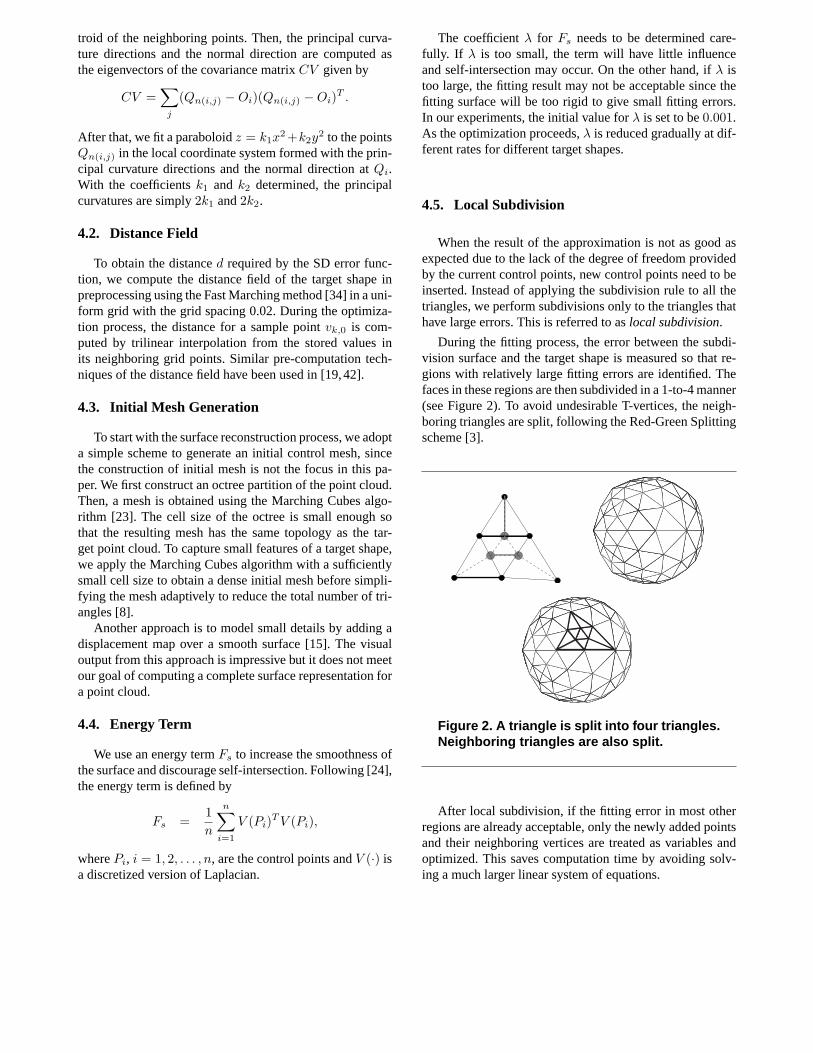
During the fitting process, the error between the subdi-vision surface and the target shape is measured so that re-gions with relatively large fitting errors are identified. Thefaces in these regions are then subdivided in a 1-to-4 manner(see Figure 2). To avoid undesirable T-vertices, the neigh-boring triangles are split, following the Red-Green Splittingscheme [3].

Figure 2. A triangle is split into four triangles.Neighboring triangles are also split.

After local subdivision, if the fitting error in most otherregions are already acceptable, only the newly added pointsand their neighboring vertices are treated as variables andoptimized. This saves computation time by avoiding solv-ing a much larger linear system of equations.

4.6. Local Modification for the Connectivity of theControl Points

The connectivity of the control points can affect the fit-ting result. Since there are a large number of combinationsof connectivity for the same set of control points and it isimpractical to enumerate and test all the combinations, weconduct an edge flip test to edges in the regions that havelarge errors (see Figure 3). An edge flip is accepted if it re-sults in a reduced error, following the strategy in [11].

Figure 3. An edge flip of a control mesh andits effect on the limit surface.

5. Results

In this section, we present experimental results to com-pare the convergence behaviors of SDM and PDM, and givetime and error statistics on some examples computed bySDM. All experiments were conducted on a PC with In-tel Xeon2.66 GHz CPU and2.00 GB RAM. The modelsare scaled into the unit cube before surface fitting.

5.1. Comparisons of SDM and PDM

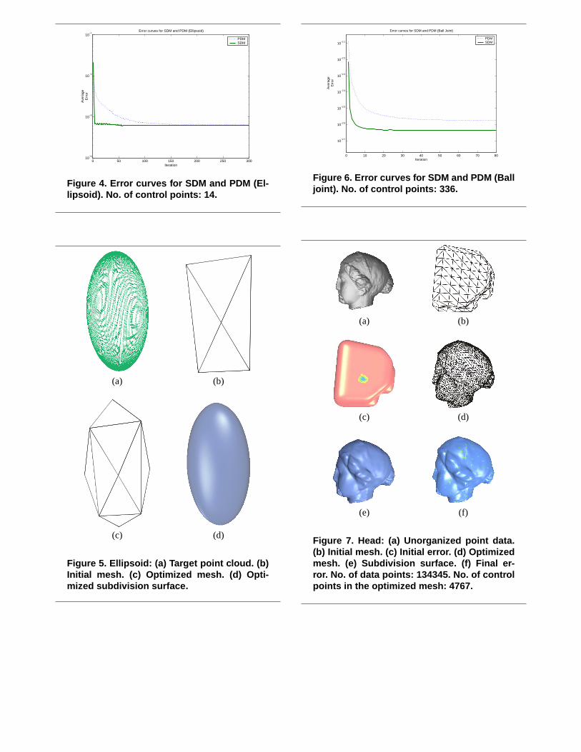
We use two data sets, the ellipsoid in Figure 5 and theball joint in Figure 8, for comparing SDM and PDM. Thecode of PDM is adapted from that of SDM by replacing theSD error function(1) by the PD error function(2). Note thatthe distance field pre-computation is still needed for PDM,but the curvature pre-computation is not. The same initialcontrol mesh is used by SDM and PDM for each of the twodata sets. Figures 4 and 6 show the error curves of SDM andPDM for the two examples. Clearly, SDM takes far fewer it-erations to attain an acceptable local minimum than PDMdoes. For the ellipsoid example, SDM converges quicklyclose to the minimum in less than10 iterations while PDMconverges to a similar value using about150 iterations. Fig-ure 5 shows the ellipsoid data, the initial mesh, and the op-timized mesh computed by SDM; the optimized mesh com-puted by PDM is similar and so is not shown.

Regarding the computational efficiency, SDM needsmuch longer time than PDM on pre-computation, since cur-vature pre-computation required by SDM is unnecessary forPDM. Our experiments show that the time used by SDM oniterative optimization is about 30% to 50% more than PDMbecause SDM needs extra time to set up the more com-plex SDM error function.

5.2. More Examples

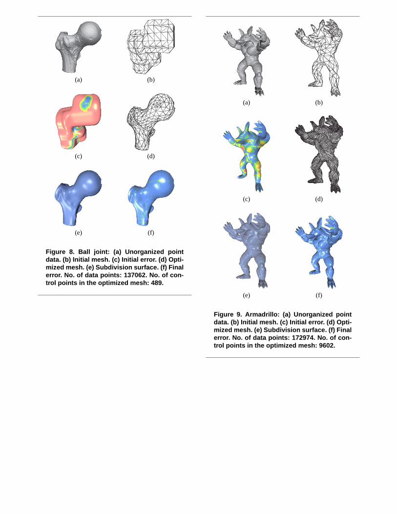
We now present three more examples to give the tim-ing and error statistics of SDM. Figures 8, 7 and 9 showthe data sets for a head, a ball joint, and an Armadrillo(data source: http://www.cyberware.com). The figures showthe unorganized point data rendered using a point renderingtechnique, the initial meshes, the optimized control meshes,and the final subdivision surfaces with color error coding.Blue, green, yellow and red represent errors in the ranges[0, 0.005), [0.005, 0.01), [0.01, 0.015) and [0.015,∞), re-spectively.

head ball joint Armadrillo

# of data points 134345 137062 172974curvature 303.33s 361.05s 550.27s

distance field 1.29s 0.71s 1.42s

Table 1. Time statistics for computing the cur-vature and the distance field. Time is mea-sured in seconds.

head ball joint Armadrillo

maximum error 0.0111 0.0090 0.0212average error 0.0023 0.0024 0.0020# of iterations 12 22 12

# of control points 4767 489 9602total time 259.98s 30.19s 623.56s

Table 2. Time and error statistics for the ex-amples. Time is measured in seconds. # ofcontrol pointsrefers to the number of verticesin the final optimized control mesh. The to-tal time does not include the time on pre-computation.

Table 1 gives the timing data for the preprocessing steps.Table 2 shows time and error statistics of SDM in comput-ing the three examples. Table 3 shows the breakdown of thetime used in the optimization step. We see in Table 3 that the

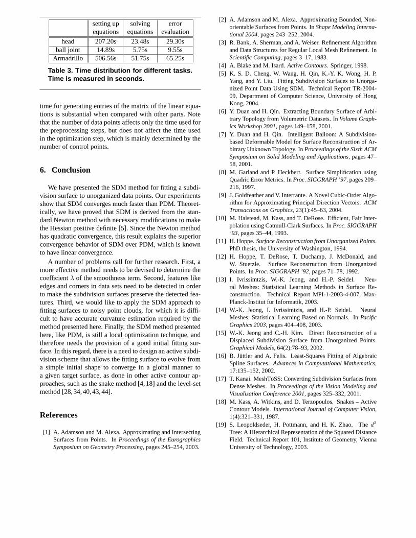
setting up solving errorequations equations evaluation

head 207.20s 23.48s 29.30sball joint 14.89s 5.75s 9.55s

Armadrillo 506.56s 51.75s 65.25s

Table 3. Time distribution for different tasks.Time is measured in seconds.

time for generating entries of the matrix of the linear equa-tions is substantial when compared with other parts. Notethat the number of data points affects only the time used forthe preprocessing steps, but does not affect the time usedin the optimization step, which is mainly determined by thenumber of control points.

6. Conclusion

We have presented the SDM method for fitting a subdi-vision surface to unorganized data points. Our experimentsshow that SDM converges much faster than PDM. Theoret-ically, we have proved that SDM is derived from the stan-dard Newton method with necessary modifications to makethe Hessian positive definite [5]. Since the Newton methodhas quadratic convergence, this result explains the superiorconvergence behavior of SDM over PDM, which is knownto have linear convergence.

A number of problems call for further research. First, amore effective method needs to be devised to determine thecoefficientλ of the smoothness term. Second, features likeedges and corners in data sets need to be detected in orderto make the subdivision surfaces preserve the detected fea-tures. Third, we would like to apply the SDM approach tofitting surfaces to noisy point clouds, for which it is diffi-cult to have accurate curvature estimation required by themethod presented here. Finally, the SDM method presentedhere, like PDM, is still a local optimization technique, andtherefore needs the provision of a good initial fitting sur-face. In this regard, there is a need to design an active subdi-vision scheme that allows the fitting surface to evolve froma simple initial shape to converge in a global manner toa given target surface, as done in other active contour ap-proaches, such as the snake method [4,18] and the level-setmethod [28,34,40,43,44].

References

[1] A. Adamson and M. Alexa. Approximating and IntersectingSurfaces from Points. InProceedings of the EurographicsSymposium on Geometry Processing, pages 245–254, 2003.

[2] A. Adamson and M. Alexa. Approximating Bounded, Non-orientable Surfaces from Points. InShape Modeling Interna-tional 2004, pages 243–252, 2004.

[3] R. Bank, A. Sherman, and A. Weiser. Refinement Algorithmand Data Structures for Regular Local Mesh Refinement. InScientific Computing, pages 3–17, 1983.

[4] A. Blake and M. Isard.Active Contours. Springer, 1998.[5] K. S. D. Cheng, W. Wang, H. Qin, K.-Y. K. Wong, H. P.

Yang, and Y. Liu. Fitting Subdivision Surfaces to Unorga-nized Point Data Using SDM. Technical Report TR-2004-09, Department of Computer Science, University of HongKong, 2004.

[6] Y. Duan and H. Qin. Extracting Boundary Surface of Arbi-trary Topology from Volumetric Datasets. InVolume Graph-ics Workshop 2001, pages 149–158, 2001.

[7] Y. Duan and H. Qin. Intelligent Balloon: A Subdivision-based Deformable Model for Surface Reconstruction of Ar-bitrary Unknown Topology. InProceedings of the Sixth ACMSymposium on Solid Modeling and Applications, pages 47–58, 2001.

[8] M. Garland and P. Heckbert. Surface Simplification usingQuadric Error Metrics. InProc. SIGGRAPH ’97, pages 209–216, 1997.

[9] J. Goldfeather and V. Interrante. A Novel Cubic-Order Algo-rithm for Approximating Principal Direction Vectors.ACMTransactions on Graphics, 23(1):45–63, 2004.

[10] M. Halstead, M. Kass, and T. DeRose. Efficient, Fair Inter-polation using Catmull-Clark Surfaces. InProc. SIGGRAPH’93, pages 35–44, 1993.

[11] H. Hoppe.Surface Reconstruction from Unorganized Points.PhD thesis, the University of Washington, 1994.

[12] H. Hoppe, T. DeRose, T. Duchamp, J. McDonald, andW. Stuetzle. Surface Reconstruction from UnorganizedPoints. InProc. SIGGRAPH ’92, pages 71–78, 1992.

[13] I. Ivrissimtzis, W.-K. Jeong, and H.-P. Seidel. Neu-ral Meshes: Statistical Learning Methods in Surface Re-construction. Technical Report MPI-1-2003-4-007, Max-Planck-Institut fur Informatik, 2003.

[14] W.-K. Jeong, I. Ivrissimtzis, and H.-P. Seidel. NeuralMeshes: Statistical Learning Based on Normals. InPacificGraphics 2003, pages 404–408, 2003.

[15] W.-K. Jeong and C.-H. Kim. Direct Reconstruction of aDisplaced Subdivision Surface from Unorganized Points.Graphical Models, 64(2):78–93, 2002.

[16] B. Juttler and A. Felis. Least-Squares Fitting of AlgebraicSpline Surfaces.Advances in Computational Mathematics,17:135–152, 2002.

[17] T. Kanai. MeshToSS: Converting Subdivision Surfaces fromDense Meshes. InProceedings of the Vision Modeling andVisualization Conference 2001, pages 325–332, 2001.

[18] M. Kass, A. Witkins, and D. Terzopoulos. Snakes – ActiveContour Models.International Journal of Computer Vision,1(4):321–331, 1987.

[19] S. Leopoldseder, H. Pottmann, and H. K. Zhao. Thed2

Tree: A Hierarchical Representation of the Squared DistanceField. Technical Report 101, Institute of Geometry, ViennaUniversity of Technology, 2003.

[20] D. Liersch, A. Sovakar, and L. Kobbelt. Parameter Reductionand Automatic Generation of Active Shape Models.Work-shop Bildverarbeitung fur die Medizin, 2003.

[21] N. Litke, A. Levin, and P. Schroder. Fitting Subdivision Sur-faces. InProc. IEEE Visualization 2001, pages 319–324,2001.

[22] C. Loop. Smooth Subdivision Surfaces based on Triangles.Master’s thesis, Department of Mathematics, University ofUtah, 1987.

[23] W. Lorensen and H. Cline. Marching Cubes: A High Resolu-tion 3-D Surface Construction Algorithm.Computer Graph-ics, 21:163–169, 1987.

[24] C. Lurig, L. Kobbelt, and T. Ertl. Hierarchical Solutions forthe Deformable Surface Problem in Visualization.Graphi-cal Models, 62:2–18, 2000.

[25] W. Ma and J. P. Kruth. Parameterization of Randomly Mea-sured Points for Least Squares Fitting of B-spline Curves andSurfaces.Computer-Aided Design, 27(9):663–675, 1995.

[26] W. Ma and N. Zhao. Catmull-Clark Surface Fitting for Re-verse Engineering Applications. InProc. GMP 2000, pages274–284, 2000.

[27] W. Ma and N. Zhao. Smooth Multiple B-spline Surface Fit-ting with Catmull-Clark Subdivision Surfaces for Extraor-dinary Corner Patches.The Visual Computer, 18:415–436,2002.

[28] R. Malladi, J. A. Sethian, and B. C. Vemuri. Shape Mod-eling with Front Propagation: A Level Set Approach.IEEETransactions on Pattern Analysis and Machine Intelligence,17(2):158–175, 1995.

[29] M. Marinov and L. Kobbelt. Optimization Techniques forApproximation with Subdivision Surfaces. InACM Sympo-sium on Solid Modeling and Applications, pages 1–10, 2004.

[30] Y. Ohtake, A. Belyaev, M. Alexa, G. Turk, and H.-P. Sei-del. Multi-level Partition of Unity Implicits. InProc. SIG-GRAPH ’03, pages 463–470, 2003.

[31] H. Pottmann and M. Hofer. Geometry of the Squared Dis-tance Function to Curves and Surfaces.Visualization andMathematics III, Springer, pages 223–244, 2003.

[32] H. Pottmann and S. Leopoldseder. A Concept for Paramet-ric Surface Fitting which avoids the Parametrization Prob-lem. Computer Aided Geometric Design, 20:343–362, 2003.

[33] H. Pottmann, S. Leopoldseder, and M. Hofer. Approxima-tion with Active B-spline Curves and Surfaces. InProc. Pa-cific Graphics 02, pages 8–25, 2002.

[34] J. A. Sethian.Level Set Methods and Fast Marching Meth-ods Evolving Interfaces in Computational Geometry, FluidMechanics, Computer Vision, and Materials Science. Cam-bridge University Press, 1999.

[35] T. Speer, M. Kuppe, and J. Hoschek. Global Reparametriza-tion for Curve Approximation.Computer Aided GeometricDesign, 15:869–877, 1998.

[36] J. Stam. Evaluation of Loop Subdivision Surfaces. InSIG-GRAPH’98 CDROM Proceedings, 1998.

[37] J. Stam. Exact Evaluation of Catmull-Clark SubdivisionSurfaces at Arbitrary Parameter Values. InProc. SIG-GRAPH’98, pages 395–404, 1998.

[38] H. Suzuki, S. Takeuchi, and T. Kanai. Subdivision SurfaceFitting to a Range of Points. InThe Seventh Pacific Confer-ence on Computer Graphics and Applications, pages 158–167, 1999.

[39] I. Tobor, P. Reuter, and C. Schlick. Efficient Reconstructionof Large Scattered Geometric Datasets using the Partition ofUnity and Radial Basis Functions.Journal of WSCG 2004,12(3):467–474, 2004.

[40] R. Whitaker. A Level-Set Approach to 3D Reconstructionfrom Range Data.The International Journal of ComputerVision, 29(3):203–231, 1998.

[41] Z. Wood, M. Desbrun, P. Schroder, and D. Breen. Semi-Regular Mesh Extraction from Volumes. InProc. IEEE Vi-sualization, pages 275–282, 2000.

[42] H. P. Yang, W. Wang, and J. G. Sun. Control Point Adjust-ment for B-spline Curve Approximation.Computer-AidedDesign, 36:639–652, 2004.

[43] H. K. Zhao, T. Chan, and S. Osher. A Variational Level SetApproach to Multiphase Motion.Journal of ComputationalPhysics, 127:179–195, 1996.

[44] H. K. Zhao, S. Osher, B. Merriman, and M. Kang. Im-plicit and Non-parametric Shape Reconstruction from Un-organized Data using a Variational Level Set Method.Com-puter Vision and Image Understanding, 80:295–319, 2000.

[45] D. Zorin. Subdivision and Multiresolution Surface Repre-sentations. PhD thesis, Caltech, Pasadena, Calif, 1997.

[46] D. Zorin, P. Schroder, A. DeRose, J. Stam, L. Kobbelt, andJ. Warren. Subdivision for Modeling and Simulation. InSIG-GRAPH ’99 Course Notes, 1999.

0 50 100 150 200 250 30010

−4

10−3

10−2

10−1

Iteration

Ave

rage

Err

or

Error curves for SDM and PDM (Ellipsoid)

PDMSDM

Figure 4. Error curves for SDM and PDM (El-lipsoid). No. of control points: 14.

(a) (b)

(c) (d)

Figure 5. Ellipsoid: (a) Target point cloud. (b)Initial mesh. (c) Optimized mesh. (d) Opti-mized subdivision surface.

0 10 20 30 40 50 60 70 80

10−2.7

10−2.6

10−2.5

10−2.4

10−2.3

10−2.2

10−2.1

Error curves for SDM and PDM (Ball Joint)

Iteration

Ave

rage

Err

or

PDMSDM

Figure 6. Error curves for SDM and PDM (Balljoint). No. of control points: 336.

(a) (b)

(c) (d)

(e) (f)

Figure 7. Head: (a) Unorganized point data.(b) Initial mesh. (c) Initial error. (d) Optimizedmesh. (e) Subdivision surface. (f) Final er-ror. No. of data points: 134345. No. of controlpoints in the optimized mesh: 4767.

(a) (b)

(c) (d)

(e) (f)

Figure 8. Ball joint: (a) Unorganized pointdata. (b) Initial mesh. (c) Initial error. (d) Opti-mized mesh. (e) Subdivision surface. (f) Finalerror. No. of data points: 137062. No. of con-trol points in the optimized mesh: 489.

(a) (b)

(c) (d)

(e) (f)

Figure 9. Armadrillo: (a) Unorganized pointdata. (b) Initial mesh. (c) Initial error. (d) Opti-mized mesh. (e) Subdivision surface. (f) Finalerror. No. of data points: 172974. No. of con-trol points in the optimized mesh: 9602.