Fitting and Registration

Fitting and Registration

Computer VisionCS 543 / ECE 549

University of Illinois

Derek Hoiem

02/14/12

Announcements

• HW 1 due today

• Early feedback form

Fitting: find the parameters of a model that best fit the data

Alignment: find the parameters of the transformation that best align matched points

Fitting and Alignment• Design challenges

– Design a suitable goodness of fit measure• Similarity should reflect application goals• Encode robustness to outliers and noise

– Design an optimization method• Avoid local optima• Find best parameters quickly

Fitting and Alignment: Methods

• Global optimization / Search for parameters– Least squares fit– Robust least squares– Iterative closest point (ICP)

• Hypothesize and test– Generalized Hough transform– RANSAC

Simple example: Fitting a line

Least squares line fitting•Data: (x1, y1), …, (xn, yn)

•Line equation: yi = m xi + b

•Find (m, b) to minimize

022 yAApA TT

dp

dE

)()()(2

1

1

12

2

11

1

2

ApApyApyy

yAp

TTT

nn

n

i ii

y

y

b

m

x

x

yb

mxE

n

i ii bxmyE1

2)((xi, yi)

y=mx+b

yAAApyAApA TTTT 1

Matlab: p = A \ y;

Modified from S. Lazebnik

Problem with “vertical” least squares• Not rotation-invariant• Fails completely for vertical

lines

Slide from S. Lazebnik

Total least squaresIf (a2+b2=1) then Distance between point (xi, yi) is

|axi + byi + c|

n

i ii dybxaE1

2)( (xi, yi)

ax+by+c=0

Unit normal: N=(a, b)

Slide modified from S. Lazebnik

proof: http://mathworld.wolfram.com/Point-LineDistance2-Dimensional.html

http://mathworld.wolfram.com/Point-LineDistance2-Dimensional.html

http://mathworld.wolfram.com/Point-LineDistance2-Dimensional.html

Total least squaresIf (a2+b2=1) then Distance between point (xi, yi) is

|axi + byi + c|

Find (a, b, c) to minimize the sum of squared perpendicular distances

n

i ii dybxaE1

2)( (xi, yi)

ax+by+c=0

n

i ii cybxaE1

2)(

Unit normal: N=(a, b)


Total least squaresFind (a, b, c) to minimize the sum of squared perpendicular distances

n

i ii dybxaE1

2)( (xi, yi)

ax+by+c=0

n

i ii cybxaE1

2)(Unit normal:

N=(a, b)

0)(21

n

i ii cybxac

Eybxay

n

bx

n

ac

n

i i

n

i i 11

ApAp TT

nn

n

i ii b

a

yyxx

yyxx

yybxxaE

2

11

1

2))()((

Solution is eigenvector corresponding to smallest eigenvalue of ATA

See details on Raleigh Quotient: http://en.wikipedia.org/wiki/Rayleigh_quotient

pp

ApAp pp ApAp

T

TTTTT minimize1 s.t.minimize


http://en.wikipedia.org/wiki/Rayleigh_quotient

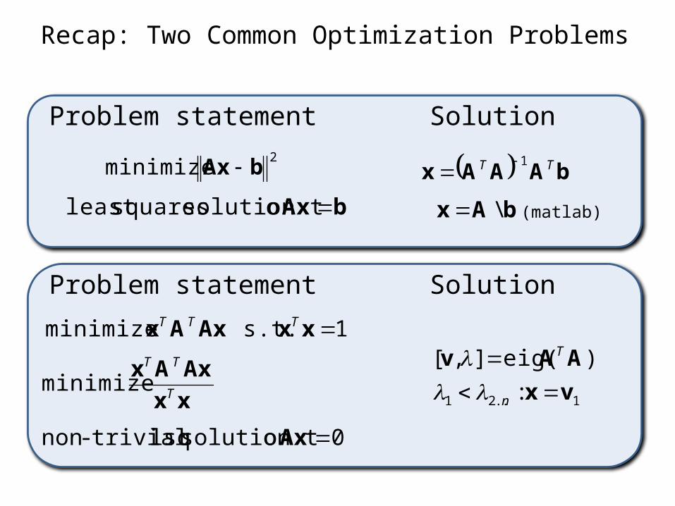
Recap: Two Common Optimization Problems

Problem statement Solution

1 s.t. minimize xxAxAx TTT

xx

AxAxT

TT

minimize

0 osolution tlsq trivial-non Ax

1..21 :

)eig(],[

vx

AAv

n

T

Problem statement Solution

bAx osolution t squaresleast bAx \

2 minimize bAx bAAAx TT 1

(matlab)

Least squares (global) optimization

Good• Clearly specified objective• Optimization is easy

Bad• May not be what you want to optimize • Sensitive to outliers

– Bad matches, extra points

• Doesn’t allow you to get multiple good fits– Detecting multiple objects, lines, etc.

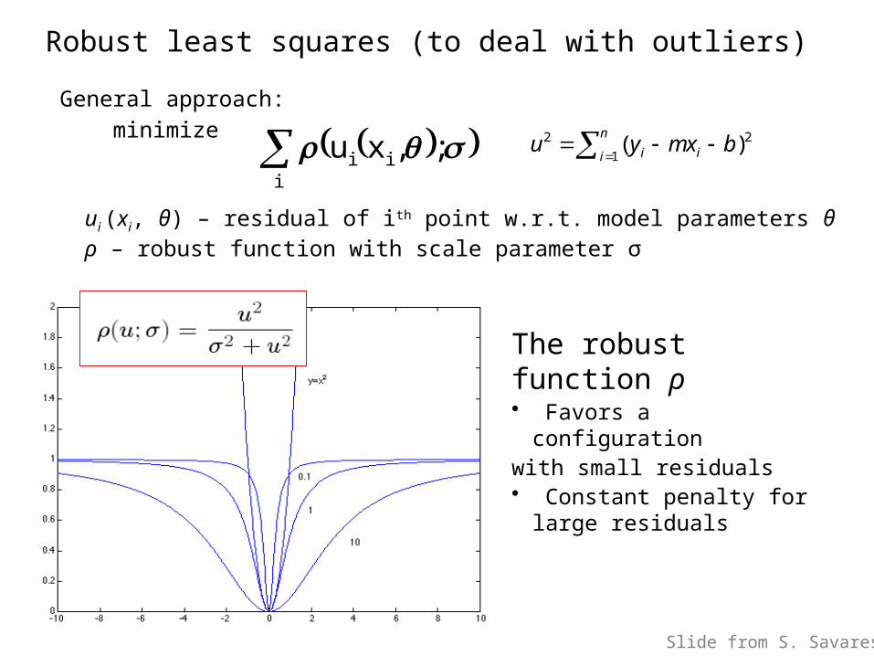
Robust least squares (to deal with outliers)General approach: minimize

ui (xi, θ) – residual of ith point w.r.t. model parameters θρ – robust function with scale parameter σ

;,xu iii

The robust function ρ • Favors a configuration with small residuals• Constant penalty for

large residuals

n

i ii bxmyu1

22 )(

Slide from S. Savarese

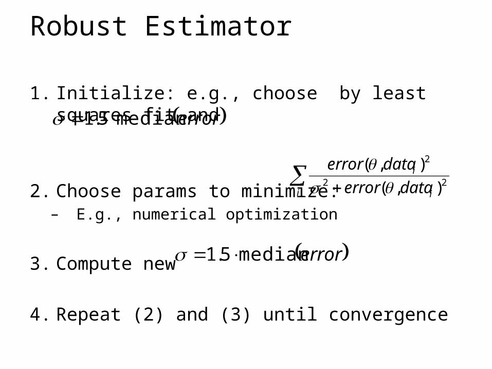
Robust Estimator

1. Initialize: e.g., choose by least squares fit and

2. Choose params to minimize:– E.g., numerical optimization

3. Compute new

4. Repeat (2) and (3) until convergence

errormedian5.1

i i

i

dataerror

dataerror22

2

),(

),(

errormedian5.1

Demo – part 1

Other ways to search for parameters (for when no closed form solution exists)• Line search

1. For each parameter, step through values and choose value that gives best fit

2. Repeat (1) until no parameter changes

• Grid search1. Propose several sets of parameters, evenly sampled in the joint

set2. Choose best (or top few) and sample joint parameters around the

current best; repeat

• Gradient descent1. Provide initial position (e.g., random)2. Locally search for better parameters by following gradient

Hypothesize and test1. Propose parameters

– Try all possible– Each point votes for all consistent parameters– Repeatedly sample enough points to solve for parameters

2. Score the given parameters– Number of consistent points, possibly weighted by

distance

3. Choose from among the set of parameters– Global or local maximum of scores

4. Possibly refine parameters using inliers

Hough Transform: Outline

1. Create a grid of parameter values

2. Each point votes for a set of parameters, incrementing those values in grid

3. Find maximum or local maxima in grid

x

y

b

m

y = m x + b

Hough transformGiven a set of points, find the curve or line that explains the data points best

P.V.C. Hough, Machine Analysis of Bubble Chamber Pictures, Proc. Int. Conf. High Energy Accelerators and Instrumentation, 1959

Hough space


x

y

b

m

x

y m3 5 3 3 2 2

3 7 11 10 4 3

2 3 1 4 5 2

2 1 0 1 3 3

b

Hough transform


x

y

Hough transformIssue : parameter space [m,b] is unbounded…

P.V.C. Hough, Machine Analysis of Bubble Chamber Pictures, Proc. Int. Conf. High Energy Accelerators and Instrumentation, 1959

Hough space

siny cosx

Use a polar representation for the parameter space


features votes

Hough transform - experiments


features votes

Need to adjust grid size or smooth


Noisy data


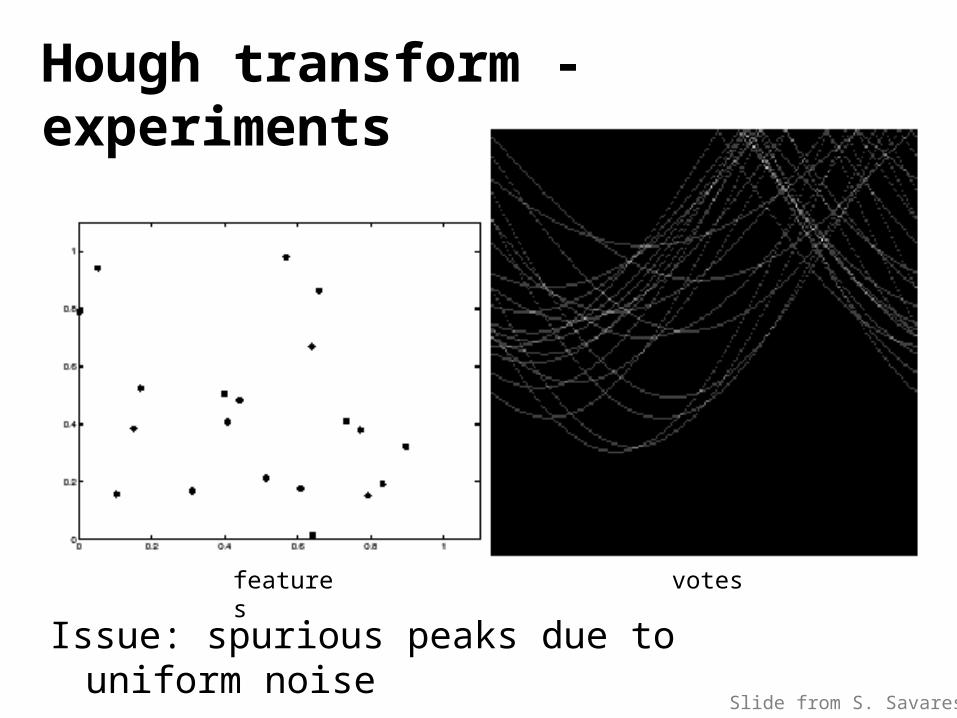
Issue: spurious peaks due to uniform noise

features votes



1. Image Canny

2. Canny Hough votes

3. Hough votes Edges

Find peaks and post-process

Hough transform example

http://ostatic.com/files/images/ss_hough.jpg

Finding lines using Hough transform• Using m,b parameterization• Using r, theta parameterization

– Using oriented gradients• Practical considerations

– Bin size– Smoothing– Finding multiple lines– Finding line segments

Finding circles (x0, y0, r) using Hough transform

• Fixed r• Variable r

Hough transform conclusionsGood• Robust to outliers: each point votes separately• Fairly efficient (much faster than trying all sets of parameters)• Provides multiple good fits

Bad• Some sensitivity to noise• Bin size trades off between noise tolerance, precision, and

speed/memory– Can be hard to find sweet spot

• Not suitable for more than a few parameters– grid size grows exponentially

Common applications• Line fitting (also circles, ellipses, etc.)• Object instance recognition (parameters are affine transform)• Object category recognition (parameters are position/scale)

RANSAC

Algorithm:

1. Sample (randomly) the number of points required to fit the model2. Solve for model parameters using samples 3. Score by the fraction of inliers within a preset threshold of the model

Repeat 1-3 until the best model is found with high confidence

Fischler & Bolles in ‘81.

(RANdom SAmple Consensus) :

RANSAC

Algorithm:

1. Sample (randomly) the number of points required to fit the model (#=2)2. Solve for model parameters using samples 3. Score by the fraction of inliers within a preset threshold of the model


Illustration by Savarese

Line fitting example

RANSAC

Algorithm:




RANSAC

6IN

Algorithm:




RANSAC

14INAlgorithm:



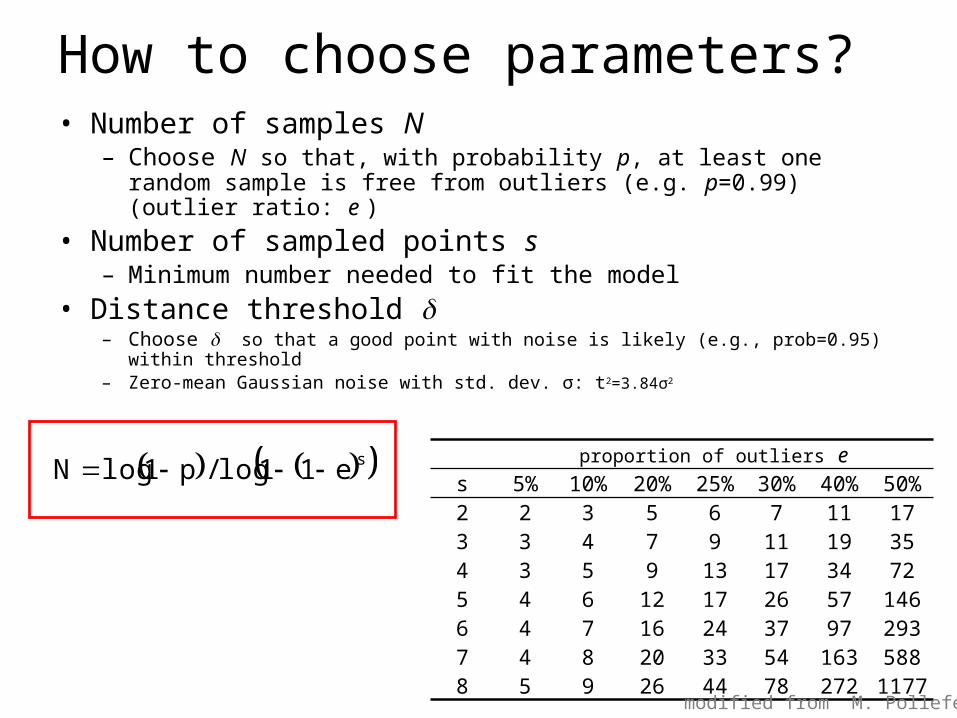
How to choose parameters?• Number of samples N

– Choose N so that, with probability p, at least one random sample is free from outliers (e.g. p=0.99) (outlier ratio: e )

• Number of sampled points s– Minimum number needed to fit the model

• Distance threshold – Choose so that a good point with noise is likely (e.g., prob=0.95) within threshold– Zero-mean Gaussian noise with std. dev. σ: t2=3.84σ2

se11log/p1logN proportion of outliers e

s 5% 10% 20% 25% 30% 40% 50%2 2 3 5 6 7 11 173 3 4 7 9 11 19 354 3 5 9 13 17 34 725 4 6 12 17 26 57 1466 4 7 16 24 37 97 2937 4 8 20 33 54 163 5888 5 9 26 44 78 272 117

7modified from M. Pollefeys

RANSAC conclusionsGood• Robust to outliers• Applicable for larger number of objective function parameters than

Hough transform• Optimization parameters are easier to choose than Hough

transform

Bad• Computational time grows quickly with fraction of outliers and

number of parameters • Not good for getting multiple fits

Common applications• Computing a homography (e.g., image stitching)• Estimating fundamental matrix (relating two views)

Demo – part 2

What if you want to align but have no prior matched pairs?

• Hough transform and RANSAC not applicable

• Important applications

Medical imaging: match brain scans or contours

Robotics: match point clouds

Iterative Closest Points (ICP) Algorithm

Goal: estimate transform between two dense sets of points

1. Initialize transformation (e.g., compute difference in means and scale)

2. Assign each point in {Set 1} to its nearest neighbor in {Set 2}

3. Estimate transformation parameters – e.g., least squares or robust least squares

4. Transform the points in {Set 1} using estimated parameters5. Repeat steps 2-4 until change is very small

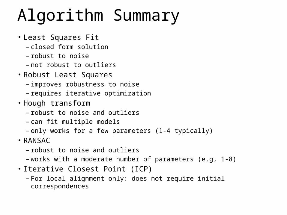
Algorithm Summary• Least Squares Fit

– closed form solution– robust to noise– not robust to outliers

• Robust Least Squares– improves robustness to noise– requires iterative optimization

• Hough transform– robust to noise and outliers– can fit multiple models– only works for a few parameters (1-4 typically)

• RANSAC– robust to noise and outliers– works with a moderate number of parameters (e.g, 1-8)

• Iterative Closest Point (ICP)– For local alignment only: does not require initial correspondences

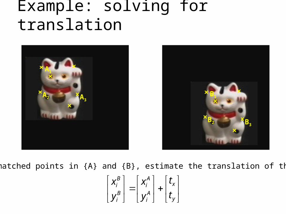
Example: solving for translation

A1

A2 A3B1

B2 B3

Given matched points in {A} and {B}, estimate the translation of the object

y

x

Ai

Ai

Bi

Bi

t

t

y

x

y

x


A1

A2 A3B1

B2 B3

Least squares solution

y

x

Ai

Ai

Bi

Bi

t

t

y

x

y

x

(tx, ty)

1. Write down objective function2. Derived solution

a) Compute derivativeb) Compute solution

3. Computational solutiona) Write in form Ax=bb) Solve using pseudo-inverse or

eigenvalue decomposition

An

Bn

An

Bn

AB

AB

y

x

yy

xx

yy

xx

t

t

11

11

10

01

10

01


A1

A2 A3B1

B2 B3

RANSAC solution

y

x

Ai

Ai

Bi

Bi

t

t

y

x

y

x

(tx, ty)

1. Sample a set of matching points (1 pair)2. Solve for transformation parameters3. Score parameters with number of inliers4. Repeat steps 1-3 N times

Problem: outliers

A4

A5

B5

B4


A1

A2 A3B1

B2 B3

Hough transform solution

y

x

Ai

Ai

Bi

Bi

t

t

y

x

y

x

(tx, ty)

1. Initialize a grid of parameter values2. Each matched pair casts a vote for

consistent values3. Find the parameters with the most votes4. Solve using least squares with inliers

A4

A5 A6

B4

B5 B6

Problem: outliers, multiple objects, and/or many-to-one matches


(tx, ty)

Problem: no initial guesses for correspondence

y

x

Ai

Ai

Bi

Bi

t

t

y

x

y

xICP solution1. Find nearest neighbors for each point2. Compute transform using matches3. Move points using transform4. Repeat steps 1-3 until convergence

Next class: Object Recognition

• Keypoint-based object instance recognition and search

Fitting and Registration

Documents

Transcript of Fitting and Registration