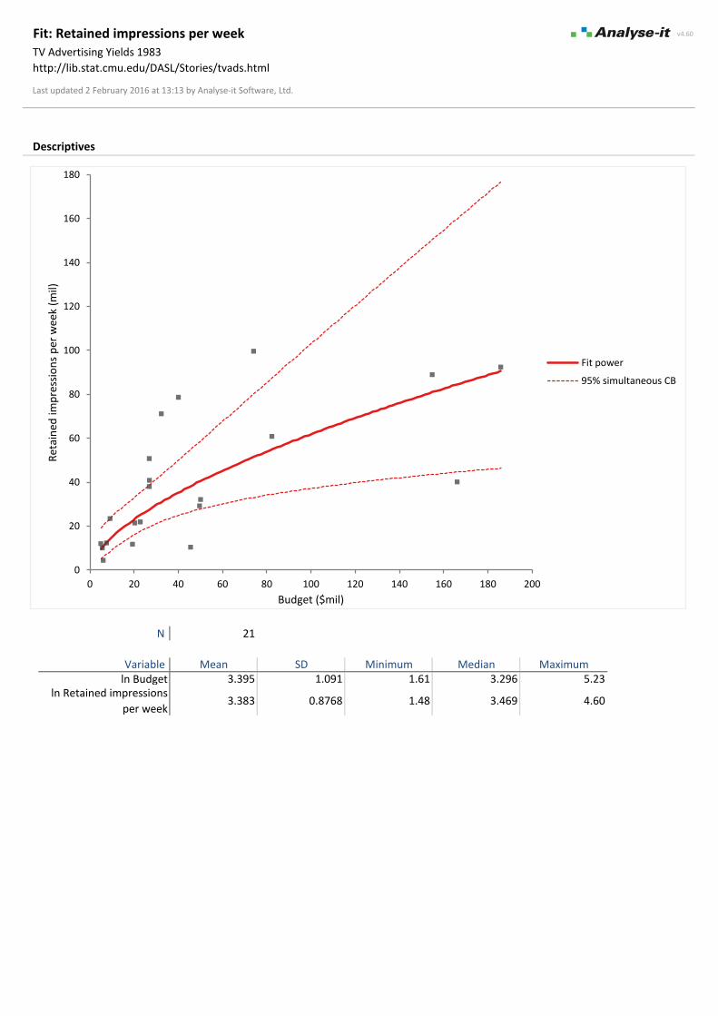
v4.60

Last updated 2 February 2016 at 13:13 by Analyse-it Software, Ltd.

Descriptives

N  21

Variable  Mean SD Minimum Median Maximumln Budget 3.395 1.091 1.61 3.296 5.23

ln Retained impressions

per week3.383 0.8768 1.48 3.469 4.60

Fit: Retained impressions per weekTV Advertising Yields 1983

http://lib.stat.cmu.edu/DASL/Stories/tvads.html

0

20

40

60

80

100

120

140

160

180

0 20 40 60 80 100 120 140 160 180 200

Ret

ain

ed im

pre

ssio

ns

per

wee

k (m

il)

Budget ($mil)

Fit power

95% simultaneous CB

v4.60

Last updated 2 February 2016 at 13:13 by Analyse-it Software, Ltd.

Fit: Retained impressions per weekTV Advertising Yields 1983

http://lib.stat.cmu.edu/DASL/Stories/tvads.html

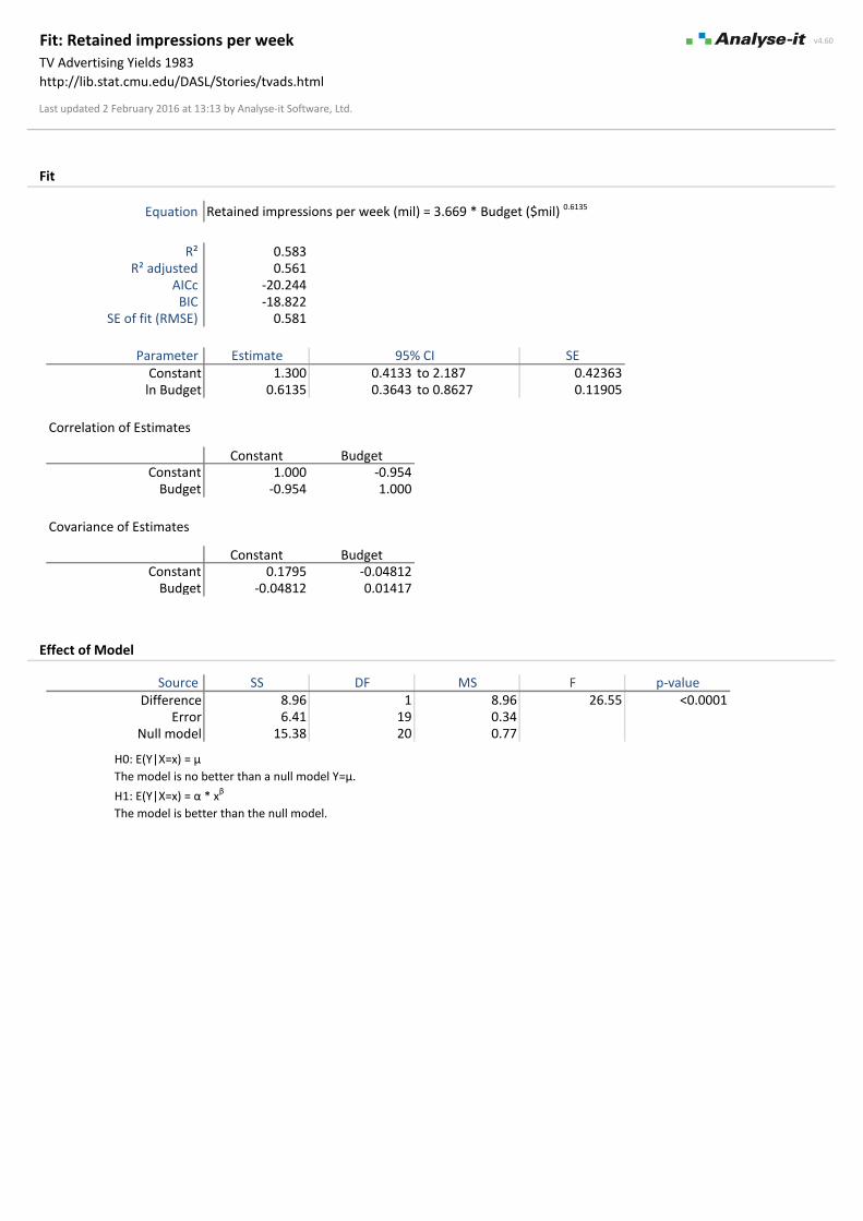
Fit

Equation 

R²  0.583R² adjusted  0.561

AICc  -20.244BIC  -18.822

SE of fit (RMSE)  0.581

Parameter  Estimate 95% CI SEConstant 1.300 0.4133 to 2.187 0.42363

ln Budget 0.6135 0.3643 to 0.8627 0.11905

Correlation of Estimates

Constant BudgetConstant 1.000 -0.954

Budget -0.954 1.000

Covariance of Estimates

Constant BudgetConstant 0.1795 -0.04812

Budget -0.04812 0.01417

Effect of Model

Source  SS DF MS F p-valueDifference 8.96 1 8.96 26.55 <0.0001

Error 6.41 19 0.34Null model 15.38 20 0.77

Retained impressions per week (mil) = 3.669 * Budget ($mil) 0.6135

H0: E(Y|X=x) = μ

The model is no better than a null model Y=μ.

H1: E(Y|X=x) = α * xβ

The model is better than the null model.

v4.60

Last updated 2 February 2016 at 13:13 by Analyse-it Software, Ltd.

Fit: Retained impressions per weekTV Advertising Yields 1983

http://lib.stat.cmu.edu/DASL/Stories/tvads.html

Residuals

-3

-2

-1

0

1

2

2.2 2.4 2.6 2.8 3 3.2 3.4 3.6 3.8 4 4.2 4.4 4.6

Stan

dar

diz

ed r

esid

ual

Predicted Y

2 2

v4.60

Last updated 2 February 2016 at 13:13 by Analyse-it Software, Ltd.

Fit: Retained impressions per weekTV Advertising Yields 1983

http://lib.stat.cmu.edu/DASL/Stories/tvads.html

Normality

Shapiro-Wilk test

W statistic  0.96p-value  0.4505

1 Do not reject the null hypothesis at the 10% significance level.

H0: F(e) = N(μ, σ)

The distribution of the population is normal with unspecified mean and standard deviation.

H1: F(e) ≠ N(μ, σ)

The distribution of the population is not normal.

-3

-2

-1

0

1

2

0 1 2 3 4 5 6 7

Stan

dar

diz

ed r

esid

ual

Frequency

-3

-2

-1

0

1

2

-3 -2 -1 0 1 2 3St

and

ard

ized

res

idu

al

Normal theoretical quantile

-3

-2

-1

0

1

2

0 4 8 12 16 20

Stan

dar

diz

ed r

esid

ual

Observation #

-3

-2

-1

0

1

2

-3 -2 -1 0 1 2

Stan

dar

diz

ed r

esid

ual

i

Standardized residual (i-1)

1

v4.60

Last updated 2 February 2016 at 13:13 by Analyse-it Software, Ltd.

Fit: Retained impressions per weekTV Advertising Yields 1983

http://lib.stat.cmu.edu/DASL/Stories/tvads.html

Outliers, Leverage, Influence

12

21

-4

-3

-2

-1

0

1

2

3

4

0.04 0.06 0.08 0.1 0.12 0.14 0.16 0.18 0.2

Stu

den

tize

d r

esid

ual

Leverage

v4.60

Last updated 2 February 2016 at 13:32 by Analyse-it Software, Ltd.

Fit

N  109

R²  0.144R² adjusted  0.067

SE of fit (RMSE)  12.85

Parameter  Estimate 95% CI SE VIFConstant 123.3 91.13 to 155.5 16.229 -

Height -0.2188 -0.4101 to -0.02747 0.096419 1.59Weight -0.01951 -0.2518 to 0.2128 0.11708 2.08

Age -0.5041 -1.163 to 0.1545 0.33194 1.12Gender: 1 0.5860 -2.567 to 3.739 1.5889 -Gender: 2 -0.5860 -3.739 to 2.567 1.5889 1.66Smokes: 1 0.3794 -3.866 to 4.625 2.1398 -Smokes: 2 -0.3794 -4.625 to 3.866 2.1398 1.10Alcohol: 1 1.251 -1.560 to 4.062 1.4167 -Alcohol: 2 -1.251 -4.062 to 1.560 1.4167 1.26

Exercise: 1 -5.539 -10.78 to -0.2948 2.6427 -Exercise: 2 1.593 -1.943 to 5.130 1.7822 1.04Exercise: 3 3.945 -0.1036 to 7.994 2.0406 1.16

Ran: 1 -0.3319 -2.855 to 2.191 1.2716 -Ran: 2 0.3319 -2.191 to 2.855 1.2716 1.04

Effect of Model

Source  SS DF MS F p-valueDifference 2757.8 9 306.4 1.86 0.0674

Error 16339.6 99 165.0Null model 19097.4 108 176.8

Fit: Pulse1Pulse rates before and after exercise

http://www.statsci.org/data/oz/ms212.html

H0: E(Y|X=x) = μ

The model is no better than a null model Y=μ.

H1: E(Y|X=x) = β0 + β1x1 + β2x2 + ...

The model is better than the null model.1 Do not reject the null hypothesis at the 5% significance level.

1

v4.60

Last updated 2 February 2016 at 13:32 by Analyse-it Software, Ltd.

Fit: Pulse1Pulse rates before and after exercise

http://www.statsci.org/data/oz/ms212.html

Effect of Terms

Term  SS DF MS F p-valueHeight 849.8 1 849.8 5.15 0.0254

Weight 4.6 1 4.6 0.03 0.8680Age 380.7 1 380.7 2.31 0.1320

Gender 22.5 1 22.5 0.14 0.7131Smokes 5.2 1 5.2 0.03 0.8596Alcohol 128.8 1 128.8 0.78 0.3792

Exercise 778.7 2 389.3 2.36 0.0998Ran 11.2 1 11.2 0.07 0.7946

2 Do not reject the null hypothesis at the 5% significance level.

H0: βTerm = 0

The term does not contribute to the model.

H1: βTerm ≠ 0

The term contributes to the model.1 Reject the null hypothesis in favour of the alternative hypothesis at the 5% significance level.

40

70

100

130

68 108 148 188

Pu

lse1

Height

27 110

Weight

18 25.5 33 40.5

Age

40

70

100

130

-0.815511 1.0244646

Pu

lse1

Gender

-0.214124 0.7507174

Smokes

-2.219436 1.7379068

Alcohol

40

70

100

130

-7.265807 4.129983

Pu

lse1

Exercise

-0.492561 0.3853459

Ran

1

2

2

2

2

2

2

2

v4.60

Last updated 2 February 2016 at 13:32 by Analyse-it Software, Ltd.

Fit: Pulse1Pulse rates before and after exercise

http://www.statsci.org/data/oz/ms212.html

Residuals

-3

-2

-1

0

1

2

3

4

5

6

55 60 65 70 75 80 85 90 95 100

Stan

dar

diz

ed r

esid

ual

Predicted Y

-3

-2

-1

0

1

2

3

4

5

6

0 8 16 24 32 40 48

Stan

dar

diz

ed r

esid

ual

Frequency

-3

-2

-1

0

1

2

3

4

5

6

-3 -2 -1 0 1 2 3

Stan

dar

diz

ed r

esid

ual

Normal theoretical quantile

v4.60

Last updated 2 February 2016 at 13:32 by Analyse-it Software, Ltd.

Fit: Pulse1Pulse rates before and after exercise

http://www.statsci.org/data/oz/ms212.html

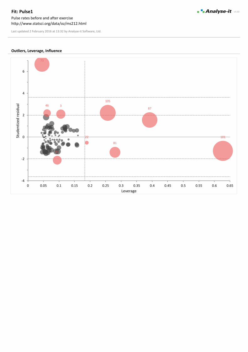
Outliers, Leverage, Influence

3

22

46

61

73

81

87

101

105

-4

-2

0

2

4

6

0 0.05 0.1 0.15 0.2 0.25 0.3 0.35 0.4 0.45 0.5 0.55 0.6 0.65

Stu

den

tize

d r

esid

ual

Leverage

v4.60

Last updated 2 February 2016 at 13:38 by Analyse-it Software, Ltd.

Fit

N  200

Parameter  Odds ratio Wald 95% CIAGE 1.044 1.016 to 1.074

SEX : 1 1.00002 0.6170 0.2533 to 1.503

SER : 1 1.00002 0.7495 0.2698 to 2.082

CAN : 1 1.00002 8.224 1.400 to 48.31

CRN : 1 1.00002 1.295 0.3573 to 4.693

INF : 1 1.00002 1.231 0.4970 to 3.048

CPR : 1 1.00002 4.770 1.107 to 20.54

SYS 0.9864 0.9730 to 0.9999HRA 0.9881 0.9713 to 1.005

PRE : 1 1.00002 1.964 0.6329 to 6.097

TYP : 1 1.00002 16.29 2.566 to 103.4

FRA : 1 1.00002 1.823 0.2910 to 11.42

PO2 : 1 1.00002 1.327 0.2815 to 6.256

PH : 1 1.00002 1.868 0.2916 to 11.97

PCO : 1 1.00002 0.3770 0.06533 to 2.175

BIC : 1 1.00002 0.7491 0.1621 to 3.463

CRE : 1 1.00002 1.643 0.2679 to 10.08

Effect of Model

Source  -LogLikelihood DF G² statistic pDifference 24.064 17 48.13 <0.0001

Fitted model 76.016 182Null model 100.08 199

Fit: STAICU

http://lib.stat.cmu.edu/DASL/LargeDatafiles/ICU.data

Φ1

H0: g(x) = β0

The model is no better than a null model Y=π.

H1: g(x) = β0 + β1x1 + β2x2 + ...

The model is better than the null model.

v4.60

Last updated 2 February 2016 at 13:38 by Analyse-it Software, Ltd.

Fit: STAICU

http://lib.stat.cmu.edu/DASL/LargeDatafiles/ICU.data

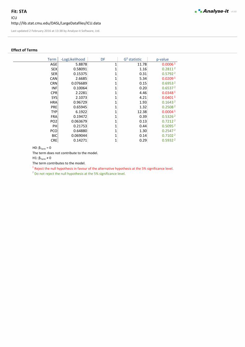
Effect of Terms

Term  -LogLikelihood DF G² statistic p-valueAGE 5.8878 1 11.78 0.0006SEX 0.58091 1 1.16 0.2811SER 0.15375 1 0.31 0.5792

CAN 2.6685 1 5.34 0.0209CRN 0.076689 1 0.15 0.6953INF 0.10064 1 0.20 0.6537

CPR 2.2281 1 4.46 0.0348SYS 2.1073 1 4.21 0.0401

HRA 0.96729 1 1.93 0.1643PRE 0.65945 1 1.32 0.2508TYP 6.1922 1 12.38 0.0004FRA 0.19472 1 0.39 0.5326PO2 0.063679 1 0.13 0.7212

PH 0.21753 1 0.44 0.5095PCO 0.64880 1 1.30 0.2547BIC 0.069044 1 0.14 0.7102

CRE 0.14271 1 0.29 0.5932

2 Do not reject the null hypothesis at the 5% significance level.

H0: βTerm = 0

The term does not contribute to the model.

H1: βTerm ≠ 0

The term contributes to the model.1 Reject the null hypothesis in favour of the alternative hypothesis at the 5% significance level.

1

2

2

1

2

2

1

1

2

2

1

2

2

2

2

2

2