Fiscal Federalism, Taxation and Grants

Martín Gonzalez-Eiras and Dirk Niepelt

Working Paper 16.05

This discussion paper series represents research work-in-progress and is distributed with the intention to foster discussion. The views herein solely represent those of the authors. No research paper in this series implies agreement by the Study Center Gerzensee and the Swiss National Bank, nor does it imply the policy views, nor potential policy of those institutions.

Fiscal Federalism, Taxation and Grants∗

Martın Gonzalez-Eiras† Dirk Niepelt‡

August 17, 2016

Abstract

We propose a theory of tax centralization and inter governmental grants inpolitico-economic equilibrium. The cost of taxation differs across levels of govern-ment because voters internalize general equilibrium effects at the central but notat the local level. This renders the degree of tax centralization and the tax burdendeterminate even if none of the traditional, expenditure-related motives for cen-tralization considered in the fiscal federalism literature is present. If central andlocal spending are complements and the trade-off between the cost of taxation andthe benefit of spending is perceived differently across levels of government, intergovernmental grants become relevant. Calibrated to U.S. data, our model helps toexplain the introduction of federal grants at the time of the New Deal, and theirincrease up to the turn of the twenty-first century. Grants are predicted to increaseto approximately 5.5% of GDP by 2060.

JEL Classification: D72, E62, H41, H77

Keywords: Fiscal policy, Federalism, Politico-economic equilibrium, Markov equi-librium, Public goods, Grants, Political Economy

1 Introduction

Whether control over fiscal policy decisions should rest with central, regional or localgovernments depends on how these governments make use of their authority. A broadbody of fiscal federalism literature has emphasized that depending on the policy task,the efficiency of policy choices may differ across levels of government. It has argued,therefore, that certain decisions are best taken de-centrally to minimize informationalor other frictions which render it difficult to cater to heterogeneous needs, while others

∗For useful comments and discussions, we thank Asger Lau Andersen, Maximilian von Ehrlich, DavidDreyer Lassen and seminar participants at CEMFI, IIBEO workshop, and Universidad Carlos III.†University of Copenhagen. Oster Farimagsgade 5, 1353 Copenhagen K, Denmark. E-mail:

mge@alum.mit.edu‡Study Center Gerzensee and University of Bern. P.O. Box 21, CH-3115 Gerzensee, Switzerland.

E-mail: dirk.niepelt@szgerzensee.ch.

1

should best be taken centrally to ensure that all important consequences of policy areinternalized.

These results have been derived with a nearly exclusive focus on government spend-ing. That the efficiency of tax collections might also differ across levels of government hasattracted much less attention although it appears equally relevant. By abstracting fromdifferences in funding efficiency the fiscal federalism literature has abstracted from an im-portant motive for decoupling revenue collection and spending across levels of government.In fact, it has typically ruled out such decoupling by assuming—counterfactually—thatgovernments individually balance their budgets.1

In this paper, we take issue with the implicit assumption in much of the literaturethat the social cost of taxation is identical across levels of government. We argue thatthere are reasons to expect the opposite and explore the implications. Most importantly,we show that if certain levels of government are in a better position to tax then this candetermine the equilibrium degree of centralization of tax collections. And if, in addition,other levels of government are in a better position to spend—as argued by the fiscalfederalism literature—then this provides a straightforward explanation for the presenceof intergovernmental transfers or grants. The specific source of cost differences we focuson is inherently dynamic2 and its implications appear consistent with the data.

The model features a central, or federal, government and many regional governmentsthat impose labor income taxes to finance the provision of public services.3 Taxation slowsdown capital accumulation and thus has general equilibrium effects: It drives up interestrates and lowers future wages which reduces the tax base in the subsequent period. Policymakers and voters at the federal level—rationally—internalize these general equilibriumeffects to the extent that they are of relevance for current voters.4 In contrast, policymakers and voters at the regional level—rationally—do not perceive general equilibriumeffects of their decisions since regions are small relative to the nation and markets arenot segmented. As a consequence, the net cost of a federal tax hike as perceived by avoter participating in national elections differs from the net cost of a regional tax hike asperceived in local elections.

Against this background, we pursue the positive questions of which level of govern-ment taxes more or less, why inter governmental grants exist, and why they have risen inprominence. Our positive analysis in the context of a dynamic model of politico-economicequilibrium contrasts with the normative approach adopted in much of the fiscal feder-alism literature. While the latter typically identifies the welfare maximizing exclusiveassignment of control to either the federal government or regional governments, we allowboth levels of government to tax and spend and solve for the politico-economic equilibrium

1The balanced budget assumption also is unrealistic because of “inter temporal decoupling,” namelybudget deficits or surpluses.

2Another obvious source relates to increasing returns in tax collections. Yet another one relates tonegative externalities of taxation; see below for a discussion of the literature on tax competition.

3We refer to a state with a multi-tier political organization as a “federal” state, and to a governmentthat makes decisions at the central level as a “federal” government. We refer to goverments makingdecisions at the local level as “regional” governments.

4The welfare consequences for yet unborn cohorts who are not represented in the political process arenot internalized.

2

with grants in a standard macroeconomic framework.5

In the model, the quantity or quality of public services depends on spending at thefederal and regional levels. We first consider a specification where federal and regionalspending are perfect substitutes and all traditional fiscal federalism considerations areabsent: Government spending does not generate externalities and preferences for publicservices are uniform across the population. In such an environment, the equilibriumdegree of centralization is indeterminate if the economy is static. But in the dynamiceconomy we consider, differential net costs of taxation render the equilibrium compositionof tax collections across levels of government determinate. Grants are irrelevant becausespending at the federal and regional level are perfect substitutes.

Next, we introduce elements emphasized in the fiscal federalism literature. Hetero-geneous preferences for public services and a restriction for the federal government todistribute resources uniformly give rise to a motive to “top up” taxes in regions with highspending needs. Cross-regional externalities from public service provision increase or de-crease federal spending depending on whether the externalities are positive or negative,but they do not affect the trade-off governing regional policy choices. In a framework withexclusive control over fiscal policy, externalities of either sign would favor centralizationfrom a welfare point of view. In our framework the federal government cannot preventspending at the regional level; all it can do is to abstain from raising taxes and fromspending.6

Finally, we relax the assumption that regional and federal government spending areperfect substitutes. With complementarities, the federal government is handicapped in itsability to affect the provision of public services because regional spending is essential. Thisrenders useful the ability to employ federal grants to increase regional spending. Whentax revenue at the federal level is “cheap,” grants allow to channel that revenue into themost productive use (regional, not only federal spending). And when externalities frompublic service provision are positive, grants allow to increase spending above the levelthat regional governments would choose in the absence of such grants. In equilibrium, thedegree of centralization of both taxes and spending is determinate and as a consequence,the size of intergovernmental grants is uniquely determined as well. Grants crowd outlocal taxation, in line with recent empirical evidence.7

While our main results are derived under the assumption that governments resort tolabor income taxation we also consider the case of capital income taxes. In contrast to theformer, capital income taxes do not affect capital accumulation once they are politicallychosen. From the perspective of federal and regional voters, the net costs of taxationthus are the same. With perfect substitutability of government spending, traditionalfiscal federalism considerations completely determine equilibrium centralization. With

5Of course, the mechanisms we emphasize would also be present in a model that adopts a normativeperspective.

6When externalities are negative, society would be better off if regional governments lowered spendingbut this is not incentive compatible.

7For example, Knight (2002) finds statistically and economically significant crowding out. He addressesidentification problems (an omitted variable bias due to the positive correlation between grant levels andunobserved preferences for public spending) by using the political power of state congressional delegationsas instruments.

3

less than perfect substitutability, grants are present when positive spending externalitiesoutweigh deadweight costs associated with the transfers. We also check whether the typeof grant—uniform or matching—makes a difference. We find that for the most part, itdoes not.

The model sheds light on the transformation of the fiscal system in the United Statesat the time of the Great Depression and the New Deal.8 Before 1933, all governmentsmainly resorted to tariffs and property taxes. After 1940, all but especially the federalgovernment, dominantly relied on income taxes, and total tax collections increased. Alsoaround 1940, federal grants rose in prominence, increasing from virtually zero in 1933to 9.4% of national expenditures in 1940.9 The model can rationalize this emergence ofgrants in parallel to the change of tax base and the rise of taxation under the assumptionthat tariffs and property taxes have a weaker effect on savings decisions than labor incometaxes.

In simulations, the model also captures the rise in the size of grants until the earlytwenty first century.10 Furthermore, it predicts grants to continue to increase up toapproximately 5.5% of GDP by 2060. In a counterfactual analysis we find that if generalequilibrium effects of taxation were not internalized at the federal level, federal taxeswould be six percentage points lower in the year 2000, regional taxes four percentagepoints higher, and grants would not be employed.

Related Literature We build on the classic analysis of fiscal federalism that featuresa trade-off between forces favoring centralization and decentralization. Oates (1972) em-phasizes externalities in the provision of public goods on the one hand, and heterogeneityof preferences across regions on the other. He finds that absent spillovers and cost-savingsfrom centralized provision, decentralization is preferable to uniform provision. But with-out information frictions, nothing prevents differentiated provision of services even in acentralized system (Oates, 1999).

Similar arguments are discussed in the theoretical political science literature (e.g.,Kincaid, 2011). A federalist governance structure allowing for multiple centers of poweris considered best suited for diverse countries, in particular if diversity is geographicallybased. Treisman (2007) critically discusses the rationales for and against political de-centralization. He argues that administrative efficiency only requires administrative, notpolitical decentralization and he questions the argument that local governments generallyare better able or motivated to extract local information.11 Our argument is related as itstresses the possible decoupling of tax and spending decisions.

The literature subsequent to Oates (1972) has offered various explanations based onpolitical economy frictions for the uniformity of centralized policy choices. For exam-ple, legislative bargaining among regional representatives at the federal level may imply

8See Wallis (2000) for a discussion of fiscal arrangements in U.S. history.9See Wallis (2000).

10Grants increased, with marked fluctuations, up to 3% of GDP in the aftermath of the Great Recession.11Treisman (2007) suggests that the most convincing arguments for the relevance of decentralization are

that it tends to increase policy stability and to lead to failures of fiscal coordination. See the discussionon tax competition below.

4

reduced sensitivity of policy to regional needs (Lockwood, 2002); differentiated centralservice provision can give rise to costly bargaining and delay and may thus be avoided(Harstad, 2007);12 credibility problems in signaling local tastes to the central governmentmay generate inefficient federal policy choices (Kessler, 2014); and centralization may in-crease accountability but must be accompanied by policy uniformity because otherwise,the central government would implement policies favoring regions that monitor more ex-tensively (Boffa, Piolatto and Ponzetto, 2016).13 Alesina and Spolaore (1997) analyze theeffect of international integration on the costs and benefits of centralization and thus, thenumber of countries.14

Wallis (2000) documents that the United States passed through distinct systems ofgovernment finance and suggests that federal, state and local governments may face dif-ferential costs to raise revenues from specific sources. Our model provides an explanationfor such cost differences based on the general equilibrium effects of taxation, and it canrationalize the change of regime during the 1930s. The notion of differential costs oftaxation due to the internalization or not of general equilibrium effects relates to Soares(2005) and Gonzalez-Eiras and Niepelt (2008) where the political support for educationor social-security financing, respectively, depends on such effects as well.15

Our work also relates to the literature on tax competition (e.g., Gordon, 1983) whichpoints out that uncoordinated local taxation of mobile factors gives rise to revenue (andother) externalities across regions. A federal government concerned with welfare at thenational level may correct these externalities by imposing federal taxes or transferringresources to regional governments through grants, among others. Our paper shares thefocus on general equilibrium effects of taxation but its perspective is positive rather thannormative. We emphasize that different perceptions about the cost of taxation at thefederal and the regional level give rise to a positive theory of fiscal federalism and mayexplain federal grants.

Uniform federal grants combined with non-uniform federal taxes (or vice versa) redis-tribute between regions and may constitute a form of inter-regional risk sharing (see, forexample, Persson and Tabellini, 1996). The fact that such risk-sharing is very commondoes not provide a rationale for federal grants, however, since risk sharing in the jointinterest of regions can be implemented without federal intervention. In our model, fiscalpolicy does not redistribute, and grants are used to achieve an allocation of resources thatregions would not choose by themselves.16

On the methodological side, our paper relates to the literature on dynamic politico-economic equilibrium (Krusell, Quadrini and Rıos-Rull, 1997). While most work in thisliterature studies equilibria with a single political decision maker Song, Storesletten and

12See also Besley and Coate (2003).13Related, Seabright (1996) argues that centralization limits the control rights of voters.14See also Bolton and Roland (1997).15See also Kotlikoff and Rosenthal (1990).16Since we are interested in explaining long run trends in U.S. fiscal policy, risk sharing considerations

are of second order. Furthermore, the absence of fiscal equalization is a natural assumption as the U.S.federal government does not use grants for this purpose. An exception is the joint financing of socialinsurance and welfare programs since the federal share of those costs increases as state income falls. SeeGruber (2011, page 266).

5

Zilibotti (2012) analyze politico-economic equilibrium in a setting with a continuum ofgovernments that take factor prices as given. We solve a dynamic game with a continuumof regional governments and a central government that internalizes general equilibriumeffects.

Outline The remainder of the paper is structured as follows. In section 2, we describethe model and in section 3, we define equilibrium. Sections 4 and 5 contain the mainanalysis and extensions, respectively. In section 6, we discuss quantitative implications ofthe model and contrast them with empirical evidence. Section 7 concludes.

2 The Model

2.1 Demographics and Institutions

We consider an economy inhabited by overlapping generations: workers and retirees.Workers supply labor, pay taxes, consume and save. In the subsequent period, theyretire, consume the return on their savings, and die. The ratio of workers to retirees inperiod t equals νt.

The economy is composed of a continuum of regions of measure one over the unitinterval. Each region is populated by a continuum of agents. The mass of agents and theirage profile is identical across regions but the preferences of agents for publicly providedservices may vary. Formally, regions are indexed by i and partitioned into J groups withgroups indexed by j. All agents in all regions in group j share the parameter γjt in theirpreference for publicly provided services. The mass of regions in group j is given by θjt ,and in every period

∑Jj=1 θ

jt = 1. The demographic, preference parameters, as well as

their cross-regional distribution follow deterministic processes.Policy decisions are taken by governments at the federal and the regional level. Federal

and regional governments act in the interest of voters participating in nationwide andregional elections, respectively. None of the governments can commit, and in each periodthey take decisions simultaneously.

2.2 Production of Final Good

A continuum of competitive firms transforms capital and labor into output. Capital isowned by retirees—it corresponds to the savings of workers in the preceding period—andfully depreciates after a period. The economy-wide capital stock per worker, kt, thereforecorresponds to the economy-wide per-capita savings of workers in the previous period,st−1, normalized by νt. Labor is supplied inelastically. The gross interest rate Rt and thewage wt are determined competitively.

We assume that the production function displays constant returns to scale such thatfactor prices in period t only depend on kt,

Rt = R(kt), wt = w(kt). (1)

6

Moreover, we assume that the elasticities of the factor prices with respect to the capital-labor ratio are independent of the latter, εRk ≡ d ln(Rt)/d ln(kt)⊥ kt, εwk ≡ d ln(wt)/d ln(kt)⊥ kt.Examples of production functions that satisfiy these assumptions include the Cobb-Douglas production function with capital share α where factor prices equal Rt = αkα−1

t

and wt = (1−α)kαt , the Ak production function, or a small open economy with exogenousfactor prices.

The independence assumption can be disposed of at the cost of loosing the ability toderive closed-form solutions.

2.3 Production and Financing of Public Services

The quantity or quality of publicly provided services (or public services, for short) in aregion i in group j, gijt , depends on public spending at the regional level and nationwide.Let eijt denote spending at the regional level and et spending by the federal government.Note that the latter occurs uniformly.17

We allow for positive or negative externalities across regions. Let ejt denote spending ina typical region in group j and let ~et ≡ (e1

t , . . . , eJt ) denote the vector that collects regional

spending across the J typical regions. (Throughout the paper, we use this notationfor cross sections.) Publicly provided services in region i in group j are a function of(eijt , ~et, et). We specify this function as

gijt = a(eijt , et)× A(~et, et)λ ∀i, j. (2)

The aggregator a(·) at the regional level and the cross-regional aggregator A(·) are increas-ing in all their arguments and the exponent λ measures the strength of the externality.In subsequent sections, we will adopt simple—and mutually consistent—functional formassumptions for a(·) and A(·). In particular, we will first consider the case without ex-ternalities, λ = 0, and with perfect substitutability between spending by the regional andfederal governments, a(eijt , et) = eijt + et, before studying more general settings.18

Spending by the federal government is financed by a labor-income tax at rate τt andspending by region i in group j is financed by a tax at rate τ ijt as well as a uniform grantfrom the federal government, xt. (See section 5 for a discussion of matching grants.) Weallow for proportional deadweight losses of grants at rate 1−σ ≥ 0. Since all governmentsbalance their budget in each period this implies

et = wt(τt − xt), eijt = wt(τijt + σxt), ejt = wt(τ

jt + σxt) ∀i, j, (3)

where τ jt denotes the regional tax rate in a typical region in group j.Tax rates and grants are non-negative.

17For rationalizations of policy uniformity at the federal level, see the literature review in the intro-duction.

18See the discussion below and appendix A for micro foundations of the general aggregator functionwe consider.

7

2.4 Preferences and Household Choices

Workers and retirees in period t value private consumption, c1,t and c2,t respectively, aswell as public services. They discount the future at factor β ∈ (0, 1). For analyticaltractability, we assume that period utility functions are logarithmic. Welfare of a workerin region i in group j who chooses savings sijt is given by

ln(cij1,t) + γjt ln(gijt ) + β(

ln(cij′

2,t+1) + Et[γj′

t+1 ln(gij′

t+1)])

s.t. cij1,t = wt(1− τt − τ ijt )− sijt , cij′

2,t+1 = sijt Rt+1.

The expectation is taken with respect to the probability that region i of type j in periodt becomes a region of type j′ in period t + 1. To streamline notation, we define ϕijt ≡(1− τt − τ ijt ) and correspondingly, ϕjt ≡ (1− τt − τ jt ).

Taking prices and taxes as given the worker optimally chooses

sijt =β

1 + βwtϕ

ijt . (4)

Conditional on prices, taxes and savings in the preceding period the welfare of a workerand a retiree, respectively, thus equal (dropping constants)

U ij,wt = (1 + β)(ln(wt) + ln(ϕijt )) + β ln(Rt+1) + γjt ln(gijt ) + βEt[γj

′

t+1 ln(gij′

t+1)], (5)

U ij,rt = ln(sij

′

t−1) + ln(Rt) + γjt ln(gijt ), (6)

where we allow for the possibility that region i of type j in period t was of type j′ inperiod t − 1. Welfare of a worker and a retiree in a typical region in group j, U j,w

t andU j,rt respectively, are defined accordingly.

2.5 Elections

Elections take place at the beginning of each period, simultaneously in all regions andnationwide. Workers and retirees may vote on candidates whose electoral platforms spec-ify values for the policy instruments as well as other characteristics like “ideology” thatare orthogonal to the fundamental policy dimensions of interest. These other characteris-tics are permanent and cannot be credibly altered in the course of electoral competition.Moreover, their valuation differs across voters (even if voters agree about the preferredpolicy platform) and is subject to random aggregate shocks, realized after candidateshave chosen their platforms. This “probabilistic-voting” setup renders the probability ofwinning a voter’s support a continuous function of the competing policy platforms. It im-plies that equilibrium policy platforms smoothly respond to changes in the demographicstructure and other fundamentals.

In the Nash equilibrium of the game with two competing candidates in a constituencychoosing platforms to maximize their expected vote shares, both candidates propose thesame policy platform.19 This platform maximizes a convex combination of the objective

19See Lindbeck and Weibull (1987) and Persson and Tabellini (2000) for discussions of probabilisticvoting.

8

functions of all groups of voters, where the weights reflect the groups’ sizes and sensitivityof voting behavior to policy changes. Those groups that care the most about policyplatforms rather than other candidate characteristics are the most likely to shift theirsupport from one candidate to the other in response to small changes in the proposedplatforms. In equilibrium, such groups of “swing voters” thus gain in political influenceand tilt policy in their own favor. If all voters are equally responsive to changes in thepolicy platforms, electoral competition implements the utilitarian optimum with respectto voters. We assume that across groups of typical regions, voters are equally responsiveto proposed changes in policy platforms. However, we allow for age related variation inresponsiveness, reflected in a per capita political influence weight of unity for young votersand a per capita weight of ω ≥ 0 for retired voters.

3 Equilibrium

3.1 Competitive Equilibrium

We focus on symmetric equilibria where all regions within the same group behave iden-tically, except possibly a set of regions of measure zero. The state is given by zt, whichincludes the exogenous demographic and preference parameters as well as the endogenousstate ~st−1.20 Conditional on zt, the production function as well as competition amongfirms determine factor prices, wt and Rt. A financing policy (~τt, τt, xt) (or policy forshort) then determines public services, ~gt, capital accumulation, ~st, and thus zt+1. Pro-ceeding recursively, a policy sequence ~τs, τs, xss≥t fully determines an allocation andprice system.

Definition 1. A competitive equilibrium conditional on z0 and a policy sequence ~τt, τt, xtt≥0

is given by an allocation and price system such that

i. capital evolves according to kt = st−1/νt, with st−1 ≡∑J

j=1 θjt−1s

jt−1, and factor

prices are determined according to (1) for all t;

ii. the government budget constraints (2) and (3) are satisfied for all t; and

iii. households optimize: (4) is satisfied for all i, j, t.

3.2 Politico-Economic Equilibrium

In politico-economic equilibrium political decision makers optimally choose the values ofthe policy instruments under their control, taking all implications of their actions intoaccount and forming rational expectations about future policy choices. We assume thatthese choices are Markov that is, they are functions of the fundamental state variables.

20In general, the state also includes the level of assets in each individual region. Logarithmic preferencesimply that the capital stock in an individual region does not affect the trade-offs faced by any politicaldecision maker, see below.

9

We conjecture and later verify that policy choices are independent of the endogenous statevariables, ~st−1. Future policy choices therefore are unaffected by current policy choices.

Political decision makers at the regional and federal level perceive the economic en-vironment differently. On the regional level they take policy choices by the federal gov-ernment and in other regions, as well as factor prices and externalities, as given. On thefederal level they take regional policy choices as given and account for the endogeneity offactor prices as well as externalities.

Formally, under the conjecture a regional decision maker in period t takes (wt, wt+1, Rt, Rt+1)as well as sijt−1 and (~τt, τt, xt, τ

ijt+1, ~τt+1, τt+1, xt+1) as given and her objective is ωU ij,r

t /νt +

U ij,wt . Effectively, she maximizes

V ijt ≡

(ω

νt+ 1

)γjt ln(a(eijt , et)) + (1 + β) ln(ϕijt ) s.t. (3). (7)

In contrast, the federal decision maker in period t takes (wt, Rt) as well as ~st−1 and(~τt, ~τt+1, τt+1, xt+1) as given and she is concerned with the average of ωU j,r

t /νt+Uj,wt across

the J groups. Effectively, she maximizes

Vt ≡J∑j=1

θjt

(ω

νt+ 1

)γjt ln(gjt ) + (1 + β) ln(ϕjt) + β ln(Rt+1) + βEt[γj

′

t+1 ln(gj′

t+1)]

(8)

s.t. (1), (2), (3), (4), kt+1 = st/νt+1.

We can now define politico-economic equilibrium (under the conjecture).21

Definition 2. A politico-economic equilibrium conditional on z0 is given by a policysequence ~τt, τt, xtt≥0 and an allocation and price system such that

i. τ ijt ≥ 0 maximizes V ijt and τ ijt = τ jt for all i, j, t;

ii. (τt, xt) ≥ 0 maximizes Vt for all t; and

iii. the allocation and price system constitute a competitive equilibrium conditional onz0 and ~τt, τt, xtt≥0.

4 Analysis

4.1 Substitutability, No Traditional Fiscal Federalism Motives

To build intuition, we start with the case where spending by the federal and the regionalgovernments are perfect substitutes, a(eijt , et) = eijt + et, and neither externalities norheterogeneity are present, λ = 0 and γjt = γt ∀j. In this case, (2) and (3) imply

gijt = wt(τijt + σxt) + wt(τt − xt) = wt(τ

ijt + τt + (σ − 1)xt) ∀i, j.

21In general, politico-economic equilibrium requires that political decision makers anticipate futurepolicy choices to be determined according to policy functions (mappings from the state into policy)and that optimal policy choices are consistent with policy functions evaluated at the state. Under theconjecture this consistency requirement is trivially satisfied.

10

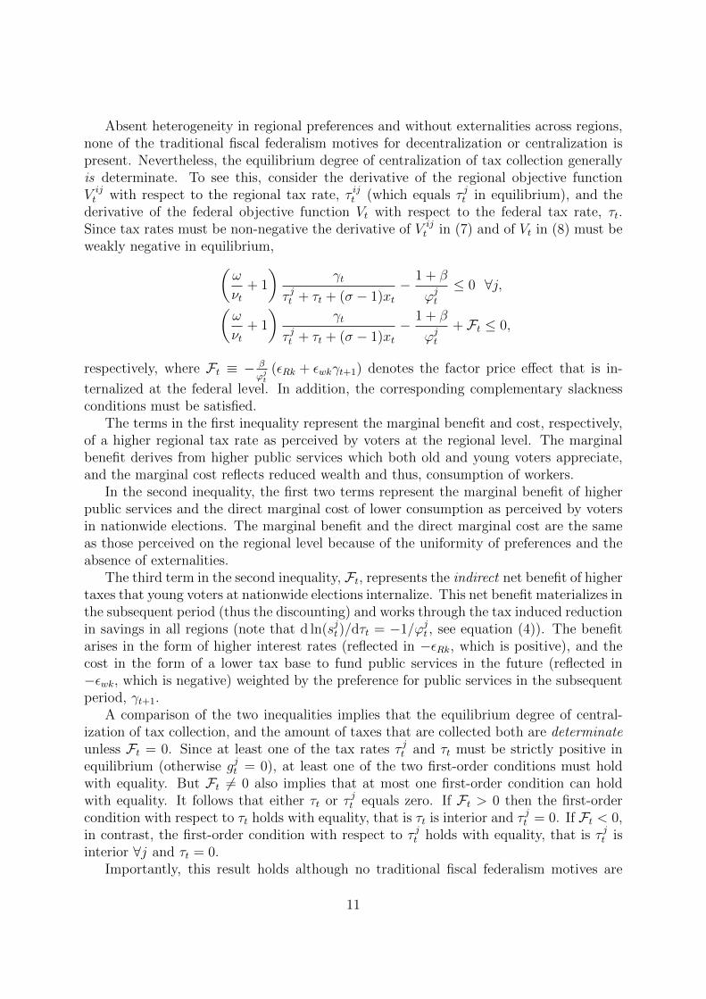
Absent heterogeneity in regional preferences and without externalities across regions,none of the traditional fiscal federalism motives for decentralization or centralization ispresent. Nevertheless, the equilibrium degree of centralization of tax collection generallyis determinate. To see this, consider the derivative of the regional objective functionV ijt with respect to the regional tax rate, τ ijt (which equals τ jt in equilibrium), and the

derivative of the federal objective function Vt with respect to the federal tax rate, τt.Since tax rates must be non-negative the derivative of V ij

t in (7) and of Vt in (8) must beweakly negative in equilibrium,(

ω

νt+ 1

)γt

τ jt + τt + (σ − 1)xt− 1 + β

ϕjt≤ 0 ∀j,(

ω

νt+ 1

)γt

τ jt + τt + (σ − 1)xt− 1 + β

ϕjt+ Ft ≤ 0,

respectively, where Ft ≡ − β

ϕjt(εRk + εwkγt+1) denotes the factor price effect that is in-

ternalized at the federal level. In addition, the corresponding complementary slacknessconditions must be satisfied.

The terms in the first inequality represent the marginal benefit and cost, respectively,of a higher regional tax rate as perceived by voters at the regional level. The marginalbenefit derives from higher public services which both old and young voters appreciate,and the marginal cost reflects reduced wealth and thus, consumption of workers.

In the second inequality, the first two terms represent the marginal benefit of higherpublic services and the direct marginal cost of lower consumption as perceived by votersin nationwide elections. The marginal benefit and the direct marginal cost are the sameas those perceived on the regional level because of the uniformity of preferences and theabsence of externalities.

The third term in the second inequality, Ft, represents the indirect net benefit of highertaxes that young voters at nationwide elections internalize. This net benefit materializes inthe subsequent period (thus the discounting) and works through the tax induced reductionin savings in all regions (note that d ln(sjt)/dτt = −1/ϕjt , see equation (4)). The benefitarises in the form of higher interest rates (reflected in −εRk, which is positive), and thecost in the form of a lower tax base to fund public services in the future (reflected in−εwk, which is negative) weighted by the preference for public services in the subsequentperiod, γt+1.

A comparison of the two inequalities implies that the equilibrium degree of central-ization of tax collection, and the amount of taxes that are collected both are determinateunless Ft = 0. Since at least one of the tax rates τ jt and τt must be strictly positive inequilibrium (otherwise gjt = 0), at least one of the two first-order conditions must holdwith equality. But Ft 6= 0 also implies that at most one first-order condition can holdwith equality. It follows that either τt or τ jt equals zero. If Ft > 0 then the first-ordercondition with respect to τt holds with equality, that is τt is interior and τ jt = 0. If Ft < 0,in contrast, the first-order condition with respect to τ jt holds with equality, that is τ jt isinterior ∀j and τt = 0.

Importantly, this result holds although no traditional fiscal federalism motives are

11

present. Determinacy results because voters at nationwide elections perceive different netbenefits of taxation than voters in regional elections. For example, when lower savingsdrive up interest rates sufficiently strongly to render Ft > 0, then the federal governmentlevies taxes because voters at nationwide elections internalize that taxation improvestheir inter temporal terms of trade. In contrast, when lower savings depress next period’swages sufficiently strongly and the preference for public services in the subsequent periodis sufficiently high to render Ft < 0, then regional governments levy taxes because onlyvoters at nationwide elections internalize the cost of taxation that results from loweringnext period’s tax base.22 A binding commitment for regions not to raise taxes wouldimprove voters’ welfare in that case.

Turning to grants, the derivative of Vt in (8) with respect to xt must be non-negativeas well, (

ω

νt+ 1

)γt(σ − 1)

τ jt + τt + (σ − 1)xt≤ 0,

and the corresponding complementary slackness condition must be satisfied. This im-plies that xt = 0 when grants entail deadweight losses (σ < 1). If σ = 1, in contrast,the equilibrium level of grants is indeterminate since perfect substitutability of spendingacross levels of government then implies that intergovernmental transfers do not affectthe allocation.

We have characterized equilibrium policy. Note that we have verified our earlier con-jecture that the policy functions are orthogonal to the endogenous state variables sincethe first-order (and complementary slackness) conditions do not involve the capital stock.We summarize these findings as our first main result:

Proposition 1. Consider the case with perfect substitutability and with no traditionalfiscal federalism motives. Suppose that εRk + εwkγt+1 6= 0 such that Ft 6= 0. Then, inequilibrium, only one level of government levies taxes. In particular, for εRk + εwkγt+1 < 0(such that Ft > 0) only the federal government levies taxes and for εRk + εwkγt+1 > 0(such that Ft < 0) only the regional governments levy taxes. Grants equal zero unlessσ = 1 in which case they are indeterminate.

Proposition 1 establishes that the equilibrium level of government that collects taxesin a federal state is determined even if none of the traditional fiscal federalism motives fordecentralization or centralization of spending is present. We study next how this resultis affected when we introduce the traditional fiscal federalism motives.

4.2 Substitutability, Traditional Fiscal Federalism Motives

Suppose next that regional preferences for public services are heterogeneous and govern-ment spending generates externalities across regions. We maintain the assumption ofperfect substitutability, a(eijt , et) = eijt + et. The conforming cross-regional aggregator

22If labor were mobile, regional governments could perceive a marginal tax increase to reduce the taxbase. Denoting by Xt this “tax competition” cost, our results would follow through, with taxation at thefederal level an equilibrium outcome as long as Ft + Xt > 0.

12

A(~et, et) is given by A(~et, et) =∑

n θnt e

nt + et and as a consequence, public services in

region i in group j equal23

gijt = w1+λt (τ ijt + τt + (σ − 1)xt)

(J∑n=1

θnt τnt + τt + (σ − 1)xt

)λ

∀i, j.

Heterogeneity and the presence of externalities do not affect the first-order conditionfor regional policy makers (except that γt is replaced by γjt ) because they take A(~et, et)as given. However, these factors do change marginal costs and benefits as perceived bydecision makers at the federal level. Heterogeneity implies that the derivative of Vt in (8)is a non-trivial average of the policy consequences across regions: The marginal benefitof higher taxes varies by region, and due to regional variation of tax rates the effect ofτt on capital accumulation works through region specific savings levels. The presence ofexternalities implies that the benefit of higher federal taxes that fund public services in aspecific region also arise outside of this region.

Let γt ≡∑

j θjtγ

tt denote the average preference for public services; τt ≡

∑j θ

jt τ

jt

the average regional tax rate; and ϕt ≡∑

j θjtϕ

jt the average tax wedge. The marginal

benefit from higher federal taxes due to spending related externalities across regions canbe expressed as Et ≡ λγt(ω/νt + 1)/(τt + τt + (σ − 1)xt) and the marginal benefit due togeneral equilibrium effects now equals Ft ≡ −β/ϕt (εRk + εwk(1 + λ)γt+1). Accordingly,the first-order conditions at the regional and federal level, respectively, now read(

ω

νt+ 1

)γjt

τ jt + τt + (σ − 1)xt− 1 + β

ϕjt≤ 0 ∀j,

J∑j=1

θjt

(ω

νt+ 1

)γjt

τ jt + τt + (σ − 1)xt− 1 + β

ϕjt

+ Et + Ft ≤ 0.

In addition, the complementary slackness conditions must be satisfied in equilibrium.Note that, under the assumption that policy functions are independent of ~st−1, the factthat region i of type j in period t might assume type j′ in period t + 1 does not affectdecisions at the local level. For the federal government the types of individual regions areirrelevant; only regional averages enter its objective function and constraints.

The two inequalities imply that total tax collections and their composition acrossgovernments continue to be determinate in equilibrium. The first inequality implies that,if the regional tax rate in a region in group j is strictly positive then the regional taxrate in all regions in groups with a stronger preference for public services must also bestrictly positive (and higher). Since at least one of the tax rates τ jt and τt must be strictlypositive in each typical region (otherwise gjt = 0), and since it is generically not possiblethat all tax rates are strictly positive24, this leaves three possibilities: First, all regionsimpose strictly positive tax rates, τ jt > 0 ∀j, and τt = 0 and Et + Ft < 0. Second, all

23Our results are robust to specifying A(~et, et) as a geometric rather than arithmetic average.24Summing the first-order conditions for regional tax rates yields the sum in the first-order condition for

the federal tax rate. Satisfying all first-order conditions with equality thus only is possible if Et +Ft = 0.

13

regions impose zero regional tax rates, τ jt = 0 ∀j, and τt > 0 and Et +Ft > 0. And third,a strict subset of regions with the strongest preference for public services imposes strictlypositive tax rates, τ jt > 0 for some but not all j, and τt > 0 and Et + Ft > 0.

The first-order condition for grants reads(ω

νt+ 1

) J∑j=1

θjtγjt (σ − 1)

τ jt + τt + (σ − 1)xt+ (σ − 1)Et ≤ 0,

which must hold in combination with the complementary slackness condition. Absentdeadweight losses, grants therefore still are irrelevant. With deadweight losses, in contrast,the situation is more nuanced. If σ < 1 and the effects due to externalities, Et, are nottoo negative then xt = 0 as before. But if σ < 1 and the effects due to externalitiesare very negative then the federal government might want to employ grants, xt > 0, asan instrument to discourage regional government spending. Since federal grants requirefederal taxes, this outcome also requires Et + Ft > 0.25

Note that again, the conjecture that policy functions are orthogonal to the endogenousstate is verified. We may therefore summarize the results as follows:

Proposition 2. Consider the case with perfect substitutability and with traditional fiscalfederalism motives. For Et + Ft > 0 the federal government levies taxes and potentially,a strict subset of regions (those groups with the highest preference for public services)levies differentiated taxes as well; grants are only used in the presence of strong negativeexternalities, unless they entail no deadweight losses. For Et +Ft < 0 all regional govern-ments levy differentiated taxes but the federal government does not; accordingly, grantsequal zero. Parametric conditions determine which case occurs. Conditional on xt, alltax rates are uniquely determined.

Proof. See appendix B for the parameter conditions under which the cases Et +Ft > 0 orEt + Ft < 0 occur, as well as the parameter condition for all regional tax rates to equalzero.

4.3 Limited Substitutability

Propositions 1 and 2 establish unique equilibrium tax rates for all governments, (~τt, τt), aslong as Ft 6= 0 or Et+Ft 6= 0, respectively. If grants are restricted to equal zero, xt = 0, asis the case in the traditional fiscal federalism literature, or when grants entail deadweightlosses, then the propositions also imply unique equilibrium spending levels for each levelof government. Absent this restriction, however, and if grants do not entail deadweightlosses the composition of spending by level of government is indeterminate.

As is clear from the discussions leading to propositions 1 and 2 the source of theirrelevance of grants (except for the odd case with strong negative externalities in propo-sition 2) is the assumption of perfect substitutability. We now relax this assumption and

25Of course, in a richer model the federal government would prefer to spend resources on other publicservices that do not generate negative externalities rather than “burning money” by means of grants.

14

introduce strict concavity in the aggregator function a(·), reflecting complementarities ingovernment spending or in the preferences for public services, or constitutional restric-tions.26 This gives a natural role to grants: When the federal government perceives amore favorable trade-off between taxation and spending than regional governments thenit transfers resources to the latter, such that regional spending increases hand in handwith federal spending.

For tractability, we assume that the aggregator function a(·) is of the Cobb-Douglasform with exponent δ on regional spending, a(eijt , et) = (eijt )δ(et)

1−δ. The conforming

cross-regional aggregator A(~et, et) is given by A(~et, et) =∏J

n=1

((ent )δ(et)

1−δ)λθnt and publicservices therefore equal

gijt = w1+λt (τ ijt + σxt)

δ(τt − xt)(1−δ)(1+λ)

J∏n=1

(τnt + σxt)δλθnt ∀i, j.

The first-order conditions with respect to a regional tax rate and the federal tax rate,respectively, now read (

ω

νt+ 1

)γjt δ

τ jt + σxt− 1 + β

ϕjt≤ 0 ∀j,

J∑j=1

θjt

(ω

νt+ 1

)γjt (1− δ)τt − xt

− 1 + β

ϕjt

+ Et + Ft ≤ 0,

where the marginal benefit from higher federal taxes due to externalities now is given byEt ≡ λγt(ω/νt + 1)(1− δ)/(τt−xt). The equilibrium factor price effects Ft are unchangedfrom before. In addition to these first-order conditions and the complementary slacknessconditions the following first-order condition for grants must be satisfied in equilibrium:

σδJ∑j=1

θjt (γjt + λγt)

τ jt + σxt− (1− δ)(1 + λ)γt

τt − xt≤ 0.

Due to the complementarities (and the restriction that xt is non-negative) the federaltax rate must be positive in equilibrium. In contrast, the regional tax rates need not bepositive unless grants equal zero.

Consider the case where all tax rates are interior, τt, τjt > 0 ∀j, such that all first-order

conditions for taxes hold with equality. To constitute an equilibrium these interior taxrates have to be consistent with the remaining equilibrium condition that the marginalbenefit of grants is weakly negative. In appendix C, we derive the parametric conditionthat must be satisfied for this to be the case. For homogeneous preferences, this condition,

26Spending complementarities could reflect informational frictions. If some governments can betterprovide certain public services than others then allocating the responsibility for spending to specificlevels of government affects the total provision. For a critique of the notion of insurmountable informationfrictions across levels of government, see Treisman (2007). In appendix A, we provide micro foundationsfor complementarities that derive from constitutional restrictions.

15

which trades-off static and dynamic externalities against deadweight losses, reduces to

β

1 + β(εRk + εwk(1 + λ)γt+1) ≥ σ(1 + λ)− 1.

If the condition is met (which is guaranteed, for example, if σ is sufficiently small) thenthe equilibrium indeed features positive tax rates at the federal level and in all regionswhile grants are absent.27 If the condition is violated, in contrast, (which is more likely,for example, if Ft or λ are sufficiently large), then tax rates cannot be strictly positive inall regions. Regions with a low valuation of public services do not levy taxes in this case,and grants are strictly positive.

Again, the conjecture that policy functions are orthogonal to the endogenous state isverified. We summarize the results as follows:

Proposition 3. Consider the case with limited substitutability and with traditional fiscalfederalism motives. The federal government always levies taxes. When the parametriccondition in appendix C is satisfied then all regions levy taxes as well, and grants generi-cally equal zero. When the opposite condition holds, then grants are strictly positive andthey fully crowd out taxes in regions with a low valuation of public services. Grants aremore likely to be used the larger general equilibrium price effects, the lower dead-weightlosses, the higher static externalities, and the larger the dispersion of preferences acrossregions.

Proof. See appendix C.

5 Extensions

5.1 Capital Income Taxes

It is instructive to compare the implications of the model under the alternative assumptionthat governments resort to capital rather than labor income taxes. At the time whencapital income taxes are decided upon and implemented, they only affect consumptionof the old, but not savings of the young (anticipated capital taxes might affect savingsbut when households take savings decisions the relevant tax rates are beyond the controlof political decision makers). As a consequence, with capital income taxation the federalgovernment perceives no equilibrium factor price effects, Ft = 0.

Maintaining the notation ϕjt for the tax wedge in a typical region of type j, the onlyother change (beyond Ft = 0) in the first order conditions for taxes concerns the weightthat governments place on the cost of taxation: (1+β) is replaced by ω

νt.28 The first-order

condition for grants is unaffected since it is independent of general equilibrium effects.

27In the non-generic case where the parametric condition is satisfied with equality, grants are indeter-minate.

28Although tax bases of labor and capital income taxes are different, implying different levels of spend-ing for a given tax rate, voters face a similar trade-off between the marginal costs and benefits of taxationsince preferences are logarithmic.

16

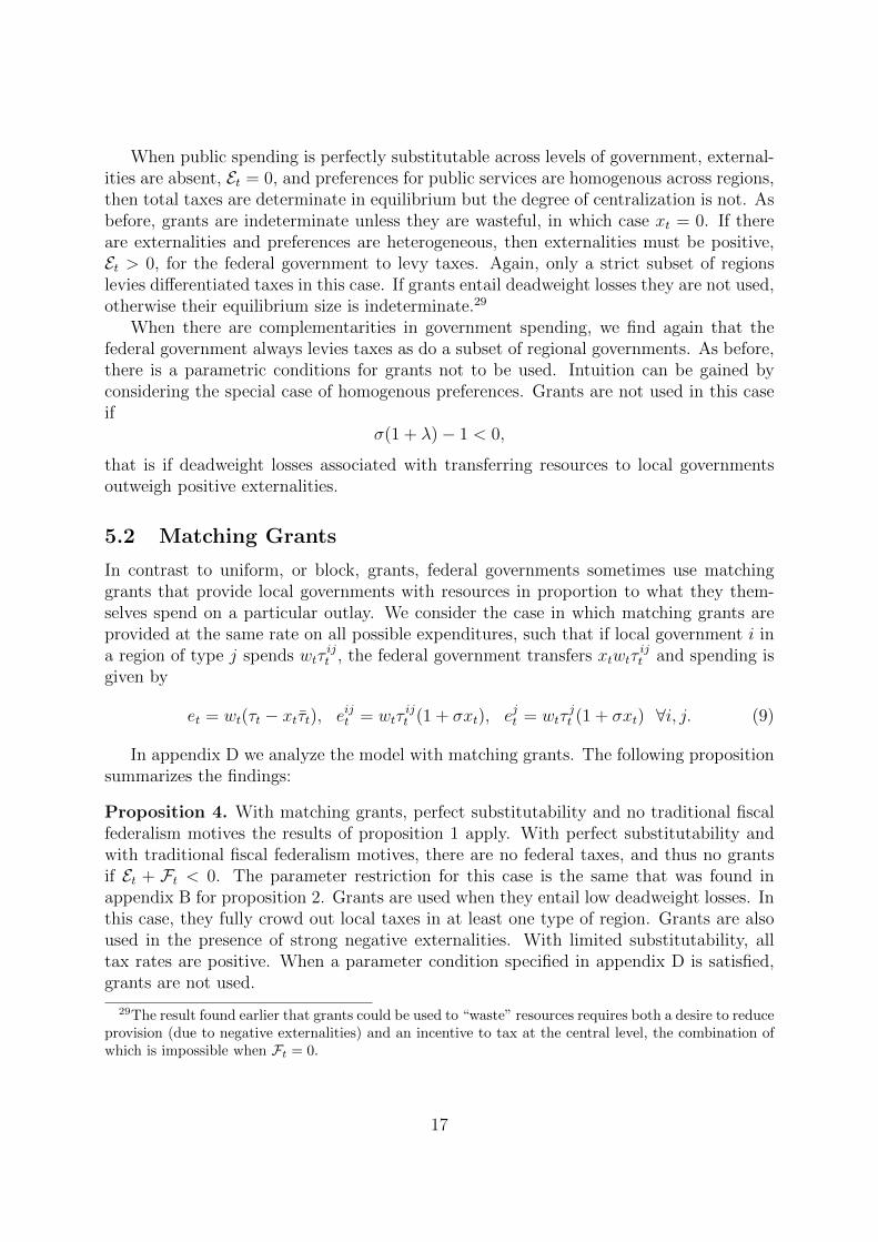
When public spending is perfectly substitutable across levels of government, external-ities are absent, Et = 0, and preferences for public services are homogenous across regions,then total taxes are determinate in equilibrium but the degree of centralization is not. Asbefore, grants are indeterminate unless they are wasteful, in which case xt = 0. If thereare externalities and preferences are heterogeneous, then externalities must be positive,Et > 0, for the federal government to levy taxes. Again, only a strict subset of regionslevies differentiated taxes in this case. If grants entail deadweight losses they are not used,otherwise their equilibrium size is indeterminate.29

When there are complementarities in government spending, we find again that thefederal government always levies taxes as do a subset of regional governments. As before,there is a parametric conditions for grants not to be used. Intuition can be gained byconsidering the special case of homogenous preferences. Grants are not used in this caseif

σ(1 + λ)− 1 < 0,

that is if deadweight losses associated with transferring resources to local governmentsoutweigh positive externalities.

5.2 Matching Grants

In contrast to uniform, or block, grants, federal governments sometimes use matchinggrants that provide local governments with resources in proportion to what they them-selves spend on a particular outlay. We consider the case in which matching grants areprovided at the same rate on all possible expenditures, such that if local government i ina region of type j spends wtτ

ijt , the federal government transfers xtwtτ

ijt and spending is

given by

et = wt(τt − xtτt), eijt = wtτijt (1 + σxt), ejt = wtτ

jt (1 + σxt) ∀i, j. (9)

In appendix D we analyze the model with matching grants. The following propositionsummarizes the findings:

Proposition 4. With matching grants, perfect substitutability and no traditional fiscalfederalism motives the results of proposition 1 apply. With perfect substitutability andwith traditional fiscal federalism motives, there are no federal taxes, and thus no grantsif Et + Ft < 0. The parameter restriction for this case is the same that was found inappendix B for proposition 2. Grants are used when they entail low deadweight losses. Inthis case, they fully crowd out local taxes in at least one type of region. Grants are alsoused in the presence of strong negative externalities. With limited substitutability, alltax rates are positive. When a parameter condition specified in appendix D is satisfied,grants are not used.

29The result found earlier that grants could be used to “waste” resources requires both a desire to reduceprovision (due to negative externalities) and an incentive to tax at the central level, the combination ofwhich is impossible when Ft = 0.

17

We conclude that the predictions of the model with uniform grants and with matchinggrants qualitatively are largely identical. The main difference to the model with uniformgrants is that with perfect substitutability and with traditional fiscal federalism motives,grants are more likely to be used when Et + Ft > 0. With limited substitutability andhomogeneous preferences, the condition for the absence of grants is given by the samecondition as in the case with uniform grants.

6 Quantitative Implications and Empirical Evidence

Wallis (2000) documents that the United States passed through three different eras ofgovernment finance. From 1790 until about 1842 state governments were the most activeand financed themselves through asset income, primarily from tolls on canals, dividendsfrom bank stock, and revenue from land sales. By 1842 several states were in default ontheir debts.

To meet this crisis, state governments resorted to property taxes and retreated frominfrastructure investments. This was met with an increase in importance of local govern-ments that also mainly resorted to property taxes for their funding. By the eve of theGreat Depression, local governments collected over half of the tax revenues raised by alllevels of government and property taxes accounted for 42% of revenues at all levels ofgovernment. During these first two eras, the federal government’s main source of revenuewere tariffs, and on a smaller scale, property taxes.

The Great Depression and the New Deal marked the birth of the current fiscal system.On the revenue side this system is characterized by the reliance on income and sales taxesat the federal and state levels.30 While income taxes only became feasible after theratification of the Sixteenth Amendment in 1913,31 and accounted for less than 10% ofall government revenues in 1933, this share rose to more than 50% by the early 1940s. Inparallel, grants grew from negligible levels before 1933 to 9.4% of federal expenditures in1940.

Summarizing this evidence from the middle of the nineteenth century onwards, wesee a transition around the time of the Great Depression from tariffs and property taxesto income taxation, alongside an increase in taxation by the federal government and theintroduction of federal grants. Wallis (2000) argues that this transition might reflect thefact that federal, state, and local governments face differential costs to raise revenues fromdifferent sources.

The model offers a potential explanation for the emergence of grants in parallel to theshift from property to income taxation. This explanation emphasizes that the ratificationof the Sixteenth Amendment in 1913 opened the way for a form of taxation—labor incometaxation—that generates general equilibrium effects and as a consequence, renders federaltaxation and grants politically more attractive.

30Income taxes include individual, corporate, and payroll taxes.31The Sixteenth Amendment states: “The Congress shall have power to lay and collect taxes on

incomes, from whatever source derived, without apportionment among the several States, and withoutregard to any census or enumeration.” In 1916 the U.S. Supreme Court upheld the constitutionality oftax legislation enacted based on this amendment.

18

1985 1990 1996 2006Obs. % in favor Obs. % in favor Obs. % in favor Obs. % in favor

Total 666 0.820 1182 0.782 1293 0.834 1483 0.633Urban 540 0.807 1014 0.775 1163 0.831 1293 0.627Rural 126 0.873 168 0.821 130 0.861 190 0.674

Table 1: Attitudes towards government spending cuts.

To check the quantitative merits of this explanation we calibrate the model withspending complementarities and simulate it. We assume that one period in the modelcorresponds to 30 years in the data, posit a Cobb-Douglas production function for thefinal good, and use the following parameter values: Based on findings in Piketty and Saez(2003) we let the capital share in the production function be 0.2815. We set νt to the30-year gross U.S. population growth rate and use Census Bureau data. From Gonzalez-Eiras and Niepelt (2008) we take ω = 0.9176. In the benchmark calibration we assumeλ = 0.

We calibrate the remaining parameters based on moment predictions of the model.We assume that there are two types of regions, “urban” and “rural,” and we proxy theshare of urban regions, θ1

t , with the average urbanization rate as reported by the CensusBureau. The motivation to distinguish regions by urban vs. rural character is twofold.On the one hand, the distinction seems relevant for observed patterns of political support.For example, Frank (2004) argues that low-income Americans living in rural areas votestrongly Republican even though the Republican party’s economic platform cuts againsttheir economic interests. We interpret this behavior as reflecting a lower preference forgovernment spending in rural areas.32 On the other hand, the distinction also seems to beborne out by survey evidence. Data on attitudes towards public spending collected by TheGeneral Social Survey in the years 1985, 1990, 1996, and 2006 indicates that respondentsin rural areas supported government spending to a lesser extent than respondents in ruralareas, see Table 1.33

The urban-vs.-rural distinction also is consistent with indirect evidence that blendsdata on state level spending and an implication of the model. Recall that the model withuniform grants predicts regions with lower valuations for public services to have a higherratio of grants relative to regional tax revenues. If urbanization is positively correlatedwith the valuation of public services, then it should go hand in hand with a decrease of

32Other observers have argued that voters care more about moral than economic issues. See An-solabehere, Rodden and Snyder Jr. (2006) for a critical discussion of the “culture war” interpretation ofthese voting patterns.

33The survey is conducted yearly by The National Data Program for the Social Sciences. Respondentswere asked if they favored or not cuts in government spending. We take the fraction of those answering“strongly in favor of” and “in favor of” as a measure of the intensity of preferences for lower spending.

19

Grants to local revenue Grants per capita

Urbanization −0.309∗ −2.66∗∗∗

(0.182) (0.981)Income per capita 0.295 2.44

(0.246) (0.700)

State FE YES YESTime FE YES YESR2 0.075 0.554Observations 98 98

Table 2: Panel regressions (robust standard errors in parenthesis, * and *** indicatesignificance at the 0.1 and 0.01 levels respectively). Urbanization is associated with alower importance of grants.

that ratio. We test this prediction using U.S. state level data for 1969 and 2008 in apanel regression of the ratio of federal grants to direct general revenue in state and localgovernments on urbanization (controlling for state income per capita), see Table 2. Asexpected, we find that an increase in urbanization is associated with a decrease in theratio of grants to state and local revenues.34

To calibrate the preference for public services as well as β, δ and σ, we use the first-order conditions for τ 1

t and xt in 1940 and τt, τ1t and xt in 2000 to match the GDP-share

of grants, the GDP-share of total (state and regional) spending, and the ratio of federalto regional spending in the year 2000, as well as the ratios of regional spending and grantsto GDP in the year 1940.35 We assume that grants are used in 1940 and 2000 such thatin those two periods regions with low valuation—rural regions—do not tax. We allowpreferences for public services to change over time at a constant rate. In addition, weuse a moment condition for the Euler equation in steady state (see Gonzalez-Eiras andNiepelt, 2008).36

34We use the following data sources: The ratio of federal grants to state and local directgeneral revenue, as well as grants per capita for 1969 are taken from Dales (1970); grants for2008 from the Census Bureau’s Consolidated Federal Funds Report for Fiscal Year 2008, Table 4(www.census.gov/prod/2009pubs/cffr-08.pdf); and state and local government finances for 2008 fromthe Census Bureau (www.census.gov/govs/local/historical data 2008.html). State income per capita rel-ative to national is taken from the Bureau of Economic Analysis (www.bea.gov/itable). Population andurbanization data comes from the Census Bureau (www.census.gov). We use 2008 data to avoid problemswith the Great Recession, and we use data for the year 1969 rather than 1970 since the table in Dales(1971) appears to contain a typo in the entry for Colorado. We exclude the District of Columbia as itsurbanization is 100% in both periods.

35Data comes from BEA.36We impose the 30-year gross interest rate R = 2.443. See Gonzalez-Eiras and Niepelt (2008) for

20

β δ γ12000 γ2

2000 γjt+1/γjt σ

0.5882 0.4915 0.7434 0.0176 1.2225 0.9365

Table 3: Calibration.

Table 3 lists the calibrated parameters. The β value corresponds to an annual discountfactor of approximately 0.982. Deadweight losses are estimated to equal around 6.4%. Thecalibration for δ suggests an almost equal role for federal and regional spending in theprovision of public services. To meet the requirement that rural areas do not levy taxesthey must have a low preference for the public service, of approximately 2.4% of thecorresponding parameter for urban areas.37

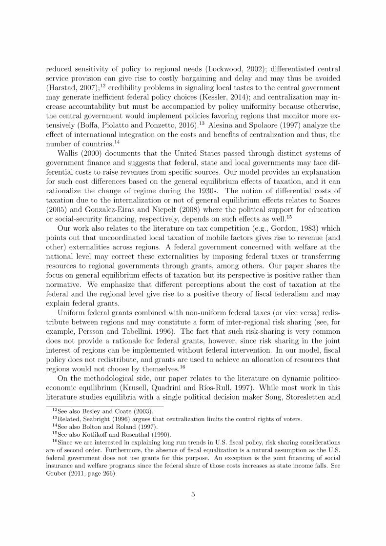
To replicate the secular increase in government spending between 1940 and 2000, themodel requires the preference for public services to grow at about 0.67% per year. This isqualitatively consistent with Wagner’s law and with the evolution over time of attitudestowards spending cuts, as reported in Table 1. If we impose θ1

t = θ2t (implying no trend

in the cross-regional distribution of preferences, as proxied by the trend in urbanization)the calibration implies a significantly higher rate of growth for the preference parametersγjt , of about 1.36% per year. This shows clearly that increased urbanization helps toexplain the data because it implies that the average valuation of public services increases.In contrast, imposing a constant population growth rate has a negligible effect on thecalibrated γjt ’s. Intuitively, in the model both workers and retirees benefit from publicservices. Ageing therefore has second order effects on the trade-off between the benefitfrom spending and the cost of taxation.

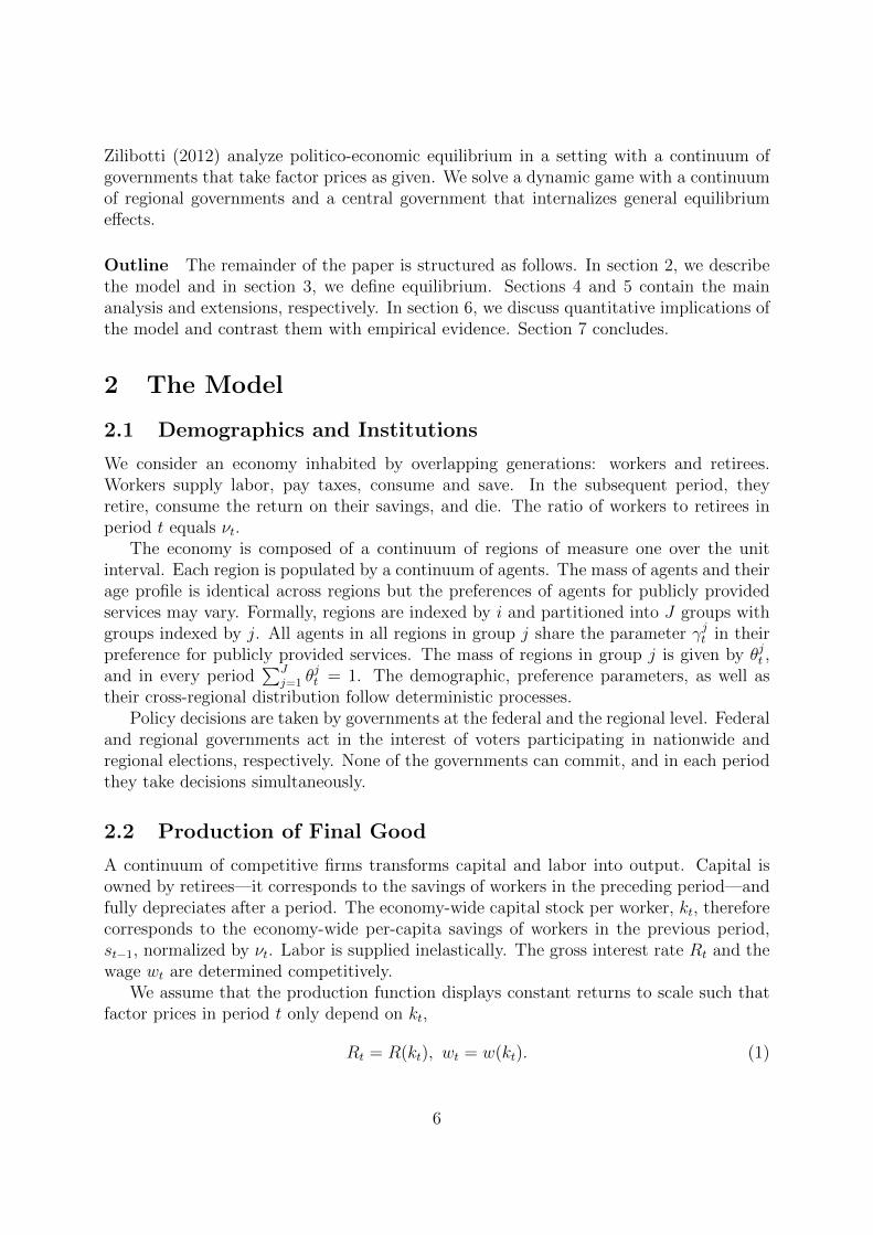
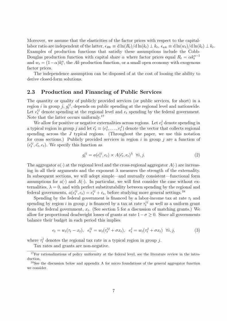
Figures 1, 2, and 3 illustrate the model predictions and make clear that the model isable to replicate the long-term trend and co-movement of the fiscal variables. In particularthe model predicts that grants would continue to increase up to approximately 5.5% ofGDP by 2060. These predictions are robust to changes in all parameters except λ andσ. When externalities are assumed to be negative, say -2%, then grants are predictedto increase to 7.3% of GDP in 2060 with regional revenue stabilized at current levels.If externalities are assumed to be positive, in contrast, say 3%, then the model predictsgrants to level off at around 4% of GDP in 2050 and regional revenue to continue increasingalmost at its current rate.

When we exogenously impose a higher value for σ (and eliminate a moment conditionin the calibration) predicted regional taxes after the year 2010 fall and predicted federaltaxes and grants strongly increase towards the end of the forecast horizon. Imposing alower value for σ generates a time series for grants that levels off and eventually reverts

details.37This feature is robust to assuming matching grants. A calibration under that assumption also requires

a large disparity in preferences across types of regions.

21

1940 1960 1980 2000 2020 2040 2060year

0.05

0.10

0.15

0.20

0.25

0.30

0.35

Total spending, share of GDP

Figure 1: Total spending: Data (circles) and model predictions (dots).

1940 1960 1980 2000 2020 2040 2060year

0.05

0.10

0.15

Average regional revenues, share of GDP

Figure 2: Regional revenues: Data (circles) and model predictions (dots).

22

1940 1960 1980 2000 2020 2040 2060year

0.02

0.04

0.06

0.08

0.10

Federal grants, share of GDP

Figure 3: Federal Grants: Data (circles) and model predictions (dots).

back to lower values. This is driven by the fact that with lower deadweight losses, thefederal government has a stronger incentive to provide grants, and these crowd out localspending.

Based on the calibration reported in table 3, we also compute a backward out-of-sampleforecast and conduct a counterfactual analysis. First, we establish that according to themodel, grants would not have been employed in the year 1910 given that mostly propertytaxes were in place and thus, general equilibrium price effects were minor. Specifically,we solve for politico-economic equilibrium in an economy with capital income taxes andshow that in this economy, in the year 1910, grants would have been absent, in line withthe data.

Second, we compute the choice of fiscal instruments in the year 2000 under the as-sumption that political decision makers at the federal level did not perceive the generalequilibrium effects of labor income taxation. We find that in this case, the federal govern-ment does not make use of grants and federal taxes are about 6 percentage points lower,partially compensated by regional taxes that are about 4 percentage points higher. Wesummarize these latter findings in table 4.

7 Concluding Remarks

What determines the degree of centralization of tax collections in a federal state? Wehave argued that differences in the perceived cost of taxation across levels of government

23

τ2000 x2000 τ2000

Baseline 0.2587 0.0333 0.1045Counterfactual 0.1858 0.0000 0.1454

Table 4: Implications of general equilibrium effects for policy outcomes.

constitute a possible candidate. While such differences may arise from various sourceswe have emphasized one that is inherently dynamic, relating to the fact that tax policyat the national level induces general equilibrium effects on interest rates and wages. Wehave also argued that in combination with traditional motives for the centralization ornot of government spending, cost differences of taxation provide a natural motive for intergovernmental grants.

Our simple framework abstracts from cross-regional insurance, redistribution, andmany other features that are present in federalist states. Given this simplicity, the pre-dictive power of the model when calibrated to match U.S. data is reassuring. Trends indemographics and urbanization can account for the increase of the GDP-shares of to-tal government spending, average regional revenues, and federal grants since the early20th century. The projected paths for the exogenous variables implies that grants as ashare of GDP will continue to increase to approximately 5.5% by 2016. A counter factualanalysis highlights the quantitative importance of general equilibrium effects. It predictsthat grants would not be used and tax rates would differ by almost 30% if the federalgovernment did not internalize these effects.

Two extensions of the model presented in this paper appear to be of particular inter-est. First, the setup could be enriched to admit productivity differences across regions,generating a role for cross-regional insurance and redistribution. Such an extension couldbe useful to study the determinants of redistributive federal grants and the consequencesof cross-regional inequality, for example in the context of German unification or Europeanintegration.

Second, the option to issue government debt for tax smoothing or tax burden shiftingpurposes could be introduced both at the federal and the regional level. Governmentswould hold conflicting views about the relative cost and benefit of public debt sinceregional policymakers do not internalize the general equilibrium effects of deficits on factorprices. As a consequence, the federal government might employ grants (and deficits) toinfluence both regional taxes and deficits. We leave these extension for future work.

24

A Derivation of Aggregator Functions

The functional form assumptions we adopt are special cases of the specification

gijt =

(∫ δ

0

(eijt (l)

δ

)κ

dl +

∫ 1

δ

(et(l)

1− δ

)κdl

) 1κ

×

(J∑n=1

θnt

(∫ δ

0

(ent (l)

δ

)κdl +

∫ 1

δ

(et(l)

1− δ

)κdl

))λκ

,

where κ ≡ (η − 1)/η and η ≥ 0. The interpretation is as follows: The public service isan aggregate that reflects spendings at the federal and the regional level on a continuumof goods indexed by l ∈ [0, 1]. We assume a constant elasticity of substitution, η ≥ 0,between types of goods (reflecting voters’ preferences or technology in the production ofthe public service). The constitution prescribes that goods with index l ∈ [0, δ] mustbe provided (but not necessarily financed) by the regional government while goods withindex l ∈ (δ, 1] must be provided by the federal government where 0 < δ < 1.38

Efficiency requires that every government provides the same amount of each goodunder its control, eijt (l) ⊥ l for all l ∈ [0, δ] and et(l) ⊥ l for all l ∈ (δ, 1] implying

gijt =

(δ

(eijtδ

)κ

+ (1− δ)(

et1− δ

)κ) 1κ

×

(J∑n=1

θnt

(δ

(entδ

)κ+ (1− δ)

(et

1− δ

)κ))λκ

.

The first term on the right-hand side of the preceding equation is defined as a(eijt , et) andthe second term as A(~et, et)

λ.For η →∞ (κ→ 1) the case of perfect substitutes follows,

gijt =(eijt + et

)×

(J∑n=1

θnt ent + et

)λ

.

The constitutional restriction (encapsulated in the parameter δ) is irrelevant in this case.For η → 0, the Leontieff case results.39 For η = 1, the Cobb-Douglas specification follows,

gijt = (eijt )δ(et)(1−δ)(1+λ)

J∏n=1

(ent )δλθnt × 1

Ψ.

In the main text we drop the constant term Ψ ≡ δδ(1+λ)(1− δ)(1−δ)(1+λ) as it is irrelevant,due to the logarithmic utility assumption.

B Proof of Proposition 2

Consider the case where all regions levy positive taxes (τ jt > 0 ∀j, first-order conditionswith respect to τ jt hold with equality), the federal government does not collect taxes

38If there were a third category of goods to which both governments could simultaneously contributethen only the government for which benefits outweigh the costs the most would contribute, due to perfectsubstitutability. As a consequence, the formulation in the text applies.

39In this case we find gijt = w1+λt min

[τt−xt

1−δ ,τ ijt +σxt

δ

]×min

[τt−xt

1−δ ,minn τ

nt +σxt

δ

]λ.

25

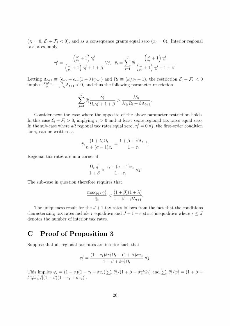
(τt = 0, Et + Ft < 0), and as a consequence grants equal zero (xt = 0). Interior regionaltax rates imply

τ jt =

(ωνt

+ 1)γjt(

ωνt

+ 1)γjt + 1 + β

∀j, τt =J∑j=1

θjt

(ωνt

+ 1)γjt(

ωνt

+ 1)γjt + 1 + β

.

Letting Λt+1 ≡ (εRk + εwk(1 + λ)γt+1) and Ωt ≡ (ω/νt + 1), the restriction Et + Ft < 0implies λγtΩt

τt− β

1−τtΛt+1 < 0, and thus the following parameter restriction

J∑j=1

θjtγjt

Ωtγjt + 1 + β

>λγt

λγtΩt + βΛt+1

.

Consider next the case where the opposite of the above parameter restriction holds.In this case Et + Ft > 0, implying τt > 0 and at least some regional tax rates equal zero.In the sub-case where all regional tax rates equal zero, τ jt = 0 ∀j, the first-order conditionfor τt can be written as

γt(1 + λ)Ωt

τt + (σ − 1)xt=

1 + β + βΛt+1

1− τt.

Regional tax rates are in a corner if

Ωtγjt

1 + β<τt + (σ − 1)xt

1− τt∀j.

The sub-case in question therefore requires that

maxj∈J γjt

γt<

(1 + β)(1 + λ)

1 + β + βΛt+1

.

The uniqueness result for the J + 1 tax rates follows from the fact that the conditionscharacterizing tax rates include r equalities and J + 1− r strict inequalities where r ≤ Jdenotes the number of interior tax rates.

C Proof of Proposition 3

Suppose that all regional tax rates are interior such that

τ jt =(1− τt)δγjtΩt − (1 + β)σxt

1 + β + δγjtΩt

∀j.

This implies ϕt = (1 + β)(1− τt + σxt)∑

j θjt/(1 + β + δγjtΩt) and

∑j θ

jt/ϕ

jt = (1 + β +

δγtΩt)/[(1 + β)(1− τt + σxt)].

26

With an interior federal tax rate the corresponding first-order condition holds withequality. Substituting the expressions above into this first-order condition yields

Ωt(1− δ)(1 + λ)γtτt − xt

=1 + β + δΩtγt + β

1+βΛt+1

(∑j

θjt1+β+δγjtΩt

)−1

1− τt + σxt.

Similarly, substituting the expressions above into the equilibrium condition for grantsyields

σ

Ωt

1 + β + δΩtγt + λγt∑

jθjt (1+β+δγjtΩt)

γjt

1− τt + σxt≤ (1 + λ)(1− δ)γt

τt − xt.

Combining the last two relations, we conclude that interior tax rates constitute an equi-librium if the following inequality on parameters is satisfied:

1 + β + δΩtγt +β

1 + βΛt+1

(∑j

θjt

1 + β + δγjtΩt

)−1

≥

σ

(1 + β + δΩtγt + λγt

∑j

θjt (1 + β + δγjtΩt)

γjt

). (10)

Only in the non-generic case in which (10) holds with an equality then positive tax ratesdo constitute an equilibrium and grants are indeterminate. If it holds strictly then themarginal benefit of grants is negative; positive tax rates do constitute an equilibrium aswell in this case and grants equal zero.

When γjt = γt ∀j, this condition simplifies to

1 + Λt+1β

1 + β≥ σ(1 + λ).

Intuitively, high deadweight losses of grants (small σ) or high indirect, general equilibriumcosts of taxation (large Λt+1) render it more likely to observe no grants and thus, strictlypositive taxes in all regions.

In the presence of heterogeneity, the cross-regional variance of the preferences forpublic services also affects the condition. A mean preserving spread of the γjt ’s reducesthe left hand side in (10) and increases the right hand side, thus making grants morelikely.

27

D Matching Grants

With matching grants and perfect substitutability the first order conditions are given by(ω

νt+ 1

)γjt (1 + σxt)

τ jt (1 + σxt) + τt − xtτt− 1 + β

ϕjt≤ 0,

∑j

θjt

(ω

νt+ 1

)γjt

τ jt (1 + σxt) + τt − xtτt− 1 + β

ϕjt

+ Et + Ft ≤ 0,

∑j

θjt(στ jt − τt)γ

jt

τ jt (1 + σxt) + τt − xtτt+

λ(σ − 1)τtγtτt(1 + (σ − 1)xt) + τt

≤ 0,

where Et = λ Ωtγtτt(1+(σ−1)xt)+τt

. When preferences are homogeneous and λ = 0, the sign of Ftdetermines whether the national or regional governments tax, as in the case of uniformgrants. Moreover, the first order condition for grants reduces to

γt(σ − 1)τ jt

τ jt (1 + (σ − 1)xt) + τt≤ 0,

implying that grants are not used if they entail deadweight losses. When σ = 1 andFt > 0 grants are irrelevant.

Consider next the case of heterogenous preferences, and possible non-zero λ. Fromthe first order conditions it is straightforward that if Et +Ft < 0, the equilibrium featurespositive taxes in all regions, the federal government collects no revenue, and thereforegrants are zero (xt = 0). Thus, the restriction Et + Ft < 0 implies λγtΩt

τt− β

1−τtΛt+1 < 0,and the following parameter restriction

J∑j=1

θjtγjt

Ωtγjt + 1 + β

>λγt

λγtΩt + βΛt+1

.

This is the same condition that we found in appendix C for uniform grants. The maindistinction with that case is that now it is not straightforward that the reverse of thecondition above, namely Et + Ft > 0, implies that at least some regional tax rates arezero. The reason for this is that the first terms in the first order condition for τt will bestrictly negative when all τ jt > 0 and xt > 0. Nevertheless, we can show that when thereare no dead-weight losses, i.e. σ = 1, grants are used and they must fully crowd out taxesin at least one region. To prove this, we start by assuming that all regional taxes arepositive. From the regional first order condition we find

τ jt =Ωtγ

jt (1 + σxt)− τt

[1 + β + Ωtγ

jt (1 + σxt)

]+ (1 + β)xtτt

(1 + σxt)[1 + β + Ωtγ

jt

] ,

and thus,

τ jt (1 + σxt) + τt − xtτt =Ωtγ

jt [(1 + σxt)− σxtτt − xtτt]

1 + β + Ωtγjt

.

28

Replacing in the first order condition for xt yields∑j θ

jt (στ

jt − τt)(1 + β + Ωtγ

jt )

Ωt [1 + σxt(1− τt)− xtτt]+

λ(σ − 1)τtγtτt(1 + (σ − 1)xt) + τt

≤ 0

If σ = 1 the left hand side reduces to

1

[1 + xt(1− τt − τt)]∑j

θjt (τjt − τt)γ

jt . (11)

Since regional taxes are increasing in γjt , (11) is strictly positive for all xt ≥ 0. Thus, thefirst order condition for grants is not satisfied if all regional tax rates are positive. Weconclude that when Et+Ft > 0 such that τt > 0, and there are no dead-weight losses fromgrants, these will be used and they crowd out regional spending in at least one type ofregion, that with the lowest γjt . By continuity the same reasoning holds when deadweightlosses are positive but small. Finally, when there are deadweight losses, and Et < 0, grantsmight be used to waste resources, as in the case with uniform grants.

With imperfect substitutability the first order conditions are given by

Ωtγjt δ

τ jt− 1 + β

ϕjt≤ 0,

∑j

θjt

Ωtγjt (1− δ)τt − xtτt

− 1 + β

ϕjt

+ Et + Ft ≤ 0,

σδ(1 + λ)γt1 + σxt

− (1− δ)(1 + λ)τtγtτt − xtτt

≤ 0.

With Et = λΩt

∑j θ

jtγjt (1−δ)τt−xtτt . Note that now all tax rates are interior, regardless of whether

there are grants in place or not, and the grant rate does not directly affect the incentivesfor regional taxes.

There will be no grants when

δσ − (1− δ)τtτt

< 0. (12)

From regional governments’ first order conditions we get τ jt =Ωtδγ

jt (1−τt)

1+β+Ωtδγjt

, and ϕjt =(1+β)(1−τt)1+β+Ωtδγ

jt

. Thus, we can calculate the following averages, and the factor price effect

∑j

θjt

ϕjt=

1 + β + Ωtδγt(1 + β)(1− τt)

,

ϕt = (1 + β)(1− τt)∑j

θjt

1 + β + Ωtδγjt

,

Ft = − βΛt+1

(1 + β)(1− τt)1∑

jθjt

1+β+Ωtδγjt

.

29

Using the above expressions to solve for τt and τt (assuming xt = 0) we get

τt =(1− δ)(1 + λ)Ωtγt

Ωtγt [δ + (1 + λ)(1− δ)] + 1 + β + β1+β

Λt+1∑j

θjt

1+β+Ωtδγjt

,

τt = (1− τt)Ωtδ∑j

θjtγjt

1 + β + Ωtδγjt

.

Replacing in (12) we have that grants will not be used if

σ(1 + λ)γt <∑j

θjtγjt

1 + β + Ωtδγjt

Ωtγtδ + 1 + β +β

1 + β

Λt+1∑j

θjt1+β+Ωtδγ

jt

.

To gain intuition we now consider the special case of homogeneous preferences. Grantswould not be used if

σ(1 + λ) < 1 +β

1 + βΛt+1.

This is the same condition that we found for the case of uniform grants.

30

References

Alesina, A. and Spolaore, E. (1997), ‘On the number and size of nations’, QuarterlyJournal of Economics 112(4), 1027–1056.

Ansolabehere, S., Rodden, J. and Snyder Jr., J. M. (2006), ‘Purple America’, Journal ofEconomic Perspectives 20(2), 97–118.

Besley, T. and Coate, S. (2003), ‘Centralized versus decentralized provision of local publicgoods: A political economy approach’, Journal of Public Economics 87(12), 2611–2637.

Boffa, F., Piolatto, A. and Ponzetto, G. A. M. (2016), ‘Political centralization and gov-ernment accountability’, Quarterly Journal of Economics 131(1), 381–422.

Bolton, P. and Roland, G. (1997), ‘The breakup of nations: A political economy analysis’,Quarterly Journal of Economics 112(4), 1057–1090.

Dales, S. R. (1970), ‘Federal grants to state and local governments 1968–1969’, SocialSecurity Bulletin 33, 31–38.

Dales, S. R. (1971), ‘Federal grants to state and local governments 1969–1970’, SocialSecurity Bulletin 34, 15–23.

Frank, T. (2004), What’s the Matter with Kansas?, Henry Holt, New York.

Gonzalez-Eiras, M. and Niepelt, D. (2008), ‘The future of social security’, Journal ofMonetary Economics 55(2), 197–218.

Gordon, R. H. (1983), ‘An optimal taxation approach to fiscal federalism’, QuarterlyJournal of Economics 98(4), 567–586.

Gruber, J. (2011), Public Finance and Public Policy, 3rd edn, Worth, New York.

Harstad, B. (2007), ‘Harmonization and side payments in political cooperation’, AmericanEconomic Review 97(3), 871–889.

Kessler, A. S. (2014), ‘Communication in federal politics: Universalism, policy unifor-mity, and the optimal allocation of fiscal authority’, Journal of Political Economy122(4), 766–805.

Kincaid, J., ed. (2011), Federalism, Sage Publications, Los Angeles.

Knight, B. (2002), ‘Endogenous federal grants and crowd-out of state government spend-ing: Theory and evidence from the federal highway aid program’, American EconomicReview 92(1), 71–92.

Kotlikoff, L. J. and Rosenthal, R. W. (1990), Some inefficiency implications of generationalpolitics and exchange, Working Paper 3354, NBER, Cambridge, Massachusetts.

31

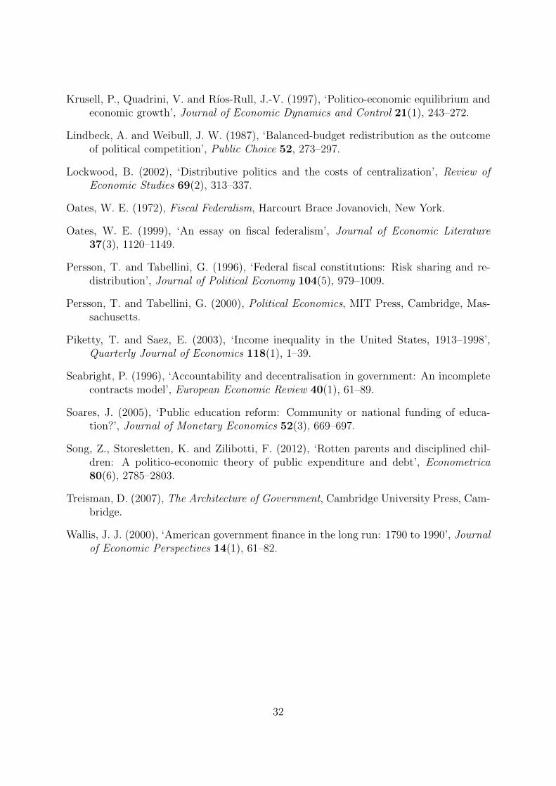
Krusell, P., Quadrini, V. and Rıos-Rull, J.-V. (1997), ‘Politico-economic equilibrium andeconomic growth’, Journal of Economic Dynamics and Control 21(1), 243–272.

Lindbeck, A. and Weibull, J. W. (1987), ‘Balanced-budget redistribution as the outcomeof political competition’, Public Choice 52, 273–297.

Lockwood, B. (2002), ‘Distributive politics and the costs of centralization’, Review ofEconomic Studies 69(2), 313–337.

Oates, W. E. (1972), Fiscal Federalism, Harcourt Brace Jovanovich, New York.

Oates, W. E. (1999), ‘An essay on fiscal federalism’, Journal of Economic Literature37(3), 1120–1149.

Persson, T. and Tabellini, G. (1996), ‘Federal fiscal constitutions: Risk sharing and re-distribution’, Journal of Political Economy 104(5), 979–1009.

Persson, T. and Tabellini, G. (2000), Political Economics, MIT Press, Cambridge, Mas-sachusetts.

Piketty, T. and Saez, E. (2003), ‘Income inequality in the United States, 1913–1998’,Quarterly Journal of Economics 118(1), 1–39.

Seabright, P. (1996), ‘Accountability and decentralisation in government: An incompletecontracts model’, European Economic Review 40(1), 61–89.

Soares, J. (2005), ‘Public education reform: Community or national funding of educa-tion?’, Journal of Monetary Economics 52(3), 669–697.

Song, Z., Storesletten, K. and Zilibotti, F. (2012), ‘Rotten parents and disciplined chil-dren: A politico-economic theory of public expenditure and debt’, Econometrica80(6), 2785–2803.

Treisman, D. (2007), The Architecture of Government, Cambridge University Press, Cam-bridge.

Wallis, J. J. (2000), ‘American government finance in the long run: 1790 to 1990’, Journalof Economic Perspectives 14(1), 61–82.

32