WP/05/221

Fiscal Dominance and Inflation in the Democratic Republic of the Congo

Jean-Claude Nachega

© 2005 International Monetary Fund WP/05/221 IMF Working Paper African Department

Fiscal Dominance and Inflation in the Democratic Republic of the Congo

Prepared by Jean-Claude Nachega1

Authorized for distribution by Arend Kouwenaar

November 2005

Abstract

This Working Paper should not be reported as representing the views of the IMF. The views expressed in this Working Paper are those of the author(s) and do not necessarily represent those of the IMF or IMF policy. Working Papers describe research in progress by the author(s) and are published to elicit comments and to further debate.

This paper examines the fiscal dominance hypothesis in the Democratic Republic of the Congo (DRC) during 1981-2003, using multivariate cointegration analysis and vector error-correction modeling. Empirical results point to strong and statistically significant long-run relationships between budget deficits and seigniorage, and between money creation and inflation. The long-run inflationary impact of budget deficits is robust to the inclusion of output growth or velocity in the inflation and monetary growth equations. The paper offers some policy recommendations for long-term price stability in the DRC. JEL Classification Numbers: E31, E60 Keywords: Congo, inflation, fiscal policy, stabilization in developing countries Author(s) E-Mail Address: jnachega@imf.org

1 I would like to thank Paul Reding, Cyrille Briançon, Chris Lane, Michael Nowak, Neil Ericsson, Fred Joutz, Maitland MacFarlan, Bergljot Barkbu, Thomson Fontaine, Arto Kovanen, Marie Nachega, Abdoul Wane, and participants at an African Department seminar for comments and discussions. Elisa Diehl provided excellent editorial assistance.

- 2 -

Contents Page

I. Introduction ……………………….…….………….......................................... 3

II. Political and Economic Background...……………………………………….... 4

III Literature Survey …………….............................................…………………... 8

IV. Theory, Methodology, and Data…….……………………………………….... 10

V. Econometric Results............................................................................................ 13

VI. Conclusions and Policy Implications………………………….......................... 30

Appendix I. Definitions and Sources of Variables………………………………….... 32

References ..................................................................................................................... 38

Tables

1. Selected Macroeconomic and Financial Indicators………………………......…... 8

2. ADF(3) Statistics for Testing for a Unit Root…........……………........................ 16 3. Cointegration Analysis of Fiscal Dominance and Inflation I............................….. 18 4. Cointegration Analysis of Fiscal Dominance and Inflation II…............................. 20 5. Cointegration Analysis of Fiscal Dominance and Inflation III................................ 21 6. Fiscal Dominance over Distinct Periods.................................................................. 23 7. Properties of VAR(1) Residuals …………………………………...……….......... 24 8. Mean and Standard Deviation of Variables…………………………………......... 25 Figures

1. Macroeconomic and Financial Indicators...................……………………............. 14 2. Error-Correction Model (ECM) for Money Growth I: Recursive Estimates and Stability Tests......................................................................................................... 33 3. ECM for Inflation I: Recursive Estimates and Stability Tests................................ 34 4. ECM for Money Growth II: Recursive Estimates and Stability Tests..................... 35 5. ECM for Inflation II: Recursive Estimates and Stability Tests............................... 36 6. Actual and Forecast Changes in Money Growth and Inflation................................ 37

- 3 -

I. INTRODUCTION

Fiscal dominance (FD), the extent to which government deficits condition the growth of the money supply, has been the prevailing regime in the Democratic Republic of the Congo (DRC)’s monetary history since its independence in June 1960. The degree of the institutional structure linking budget deficits to money creation has changed over time. Immediately following independence, civil turmoil and strong secessionist tendencies exhausted fiscal sources of revenue, forcing the government to rely on seigniorage.2 The period from 1965 to the mid-1970s was characterized by relative political stability, resulting in lower monetization of the deficit and lower inflation. Public finance exerted a stronger influence on monetary policy, first during the second half of the 1970s and in the 1980s and later in the 1990s, when FD reached its highest point. In 2001-03, FD continued but operated in the opposite direction. To meet the provisions of the IMF’s staff-monitored program (SMP) and, later, to qualify for an IMF-supported program under the Poverty Reduction and Growth Facility (PRGF), Congolese policymakers drastically curtailed budget deficits, granted independence to the central bank, unified the foreign exchange market, and liberalized key sectors of the economy. By end-2003, the orthodox stabilization had brought inflation down from triple to single digits, while overall and per capita real GDP growth became positive for two consecutive years.

The empirical relationship between budget deficits and inflation has been investigated extensively for both industrial and developing countries, with mixed results. It has often been argued that high inflation in developing countries results when a fiscally dominant government runs large and persistent budget deficits that it finances through money creation (“FD hypothesis”). It has also been recognized that, in developing countries, autonomous nonfiscal real disturbances or high inflation may erode real tax revenues and increase the real deficit in such a way that both the money supply and the deficit may be endogenous to the inflationary process.3 It follows that the endogeneity or exogeneity status of the money supply and the deficit with respect to inflation has to be determined empirically. In the case of the DRC, Beaugrand (1997) and Akitoby (2004) have studied the fiscal deficit-inflation link in a single-equation context. Not only does this approach fail to account for the potential feedback from inflation and nonfiscal real disturbances to the fiscal deficit; it also fails to establish empirically the direction of causality in this relationship.4 Moreover, Akitoby applies an ordinary least squares (OLS) regression to nonstationary time-series data but does not formally test for cointegration, thereby ignoring the spurious regression problem.

2 Seigniorage is the real revenues collected by the government through money creation.

3 See Olivera (1967), Aghevli and Khan (1977), Tanzi (1977), and Taylor (1983).

4 Akitoby uses annual data over 1990-2000 to study the deficit-inflation nexus but treats the deficit (and income velocity) as strictly exogenous. Beaugrand uses monthly data over June 1990-June 1996 to estimate price equations under both rational and adaptive expectations but acknowledges that “neither regression (results) is (are) acceptable.”

- 4 -

Beaugrand transforms his variables in first differences to render them stationary, thereby removing any information about the long run.

This study uses systems cointegration analysis to test the FD hypothesis in the DRC, a developing country that, during the past two decades, has experienced persistent budget deficits, a rapidly increasing money supply, high inflation and hyperinflation, and severe output decline. The paper empirically models inflation as a fiscally driven monetary phenomenon, and pays attention to economic theory, nonstationarity and cointegration, data congruency of the specification, parameter constancy, and exogeneity. Weak exogeneity of the budget deficit is not imposed a priori but is established within the empirical model. The empirical results point to strong and statistically significant long-term relationships between budget deficits and money growth and between money creation and inflation. This effect is robust to the inclusion of output growth or velocity in the long-run inflation equation, and we are able to confirm that the FD hypothesis holds in the DRC over the sample period covered (1981-2003). We also find that the degree of FD has evolved over time such that there appears to be a structural break around 1991 in the relationship among deficits, money creation, and inflation. We exploit this break in estimating structural vector error-correction models (SVECMs) of inflation and money creation over the periods 1982-90 and 1991-2003. We find that although the FD hypothesis holds over both periods, it intensified during the latter period. In addition, deviations of real money balances from their long-run equilibrium level and changes in output growth are shown to have played, directly or indirectly (through the money supply), significant roles in the short-run dynamics of inflation. Furthermore, recursive estimates point to significant reductions in the effects of the fiscal deficit on the money supply process during the 2001-03 stabilization period. This finding is exploited to show that the estimated model over the 1981-90 period performs well in forecasting inflation during 2001-03.

The outline of the paper is as follows. Section II presents the historical background of the DRC's present economy. Section III discusses some theoretical considerations and the empirical methodology. Section IV provides a literature survey. Section V discusses the econometric results. Section VI provides conclusions and draws some policy implications.

II. POLITICAL AND ECONOMIC BACKGROUND

A. The 1960-65 Period

The history of the DRC is one of political instability and dismal economic performance despite a remarkably rich resource base. Following independence in June 1960 and the appointment of Joseph Kasavubu and Patrice Emery Lumumba as president and prime minister, respectively, the country experienced civil turmoil. Because of its vast resources, huge size, and strategic location at the center of Africa, Congo became a hot spot in the conflict between the Soviet Union and the West during the Cold War. The ousting (and 1961 assassination) of Prime Minister Lumumba and secessionist attempts by Katanga, Kasai, Haut-Congo, and Kivu provinces led to a civil war lasting five years. The de facto independence of the mineral-rich Katanga province deprived the central government of significant tax revenue, particularly from the Belgian-controlled “Union Minière du Haut

- 5 -

Katanga,” whose mineral production had accounted for more than 60 percent of export revenue. During this five-year period, inflation, fueled by the monetary financing of the budget deficit, averaged 31 percent yearly, while nonmining output declined, with commercial agriculture and transportation services falling by a third.5 On November 24, 1965, the stalemate ended with a military takeover under the leadership of General Joseph Desiré Mobutu.

B. The 1965-89 Period

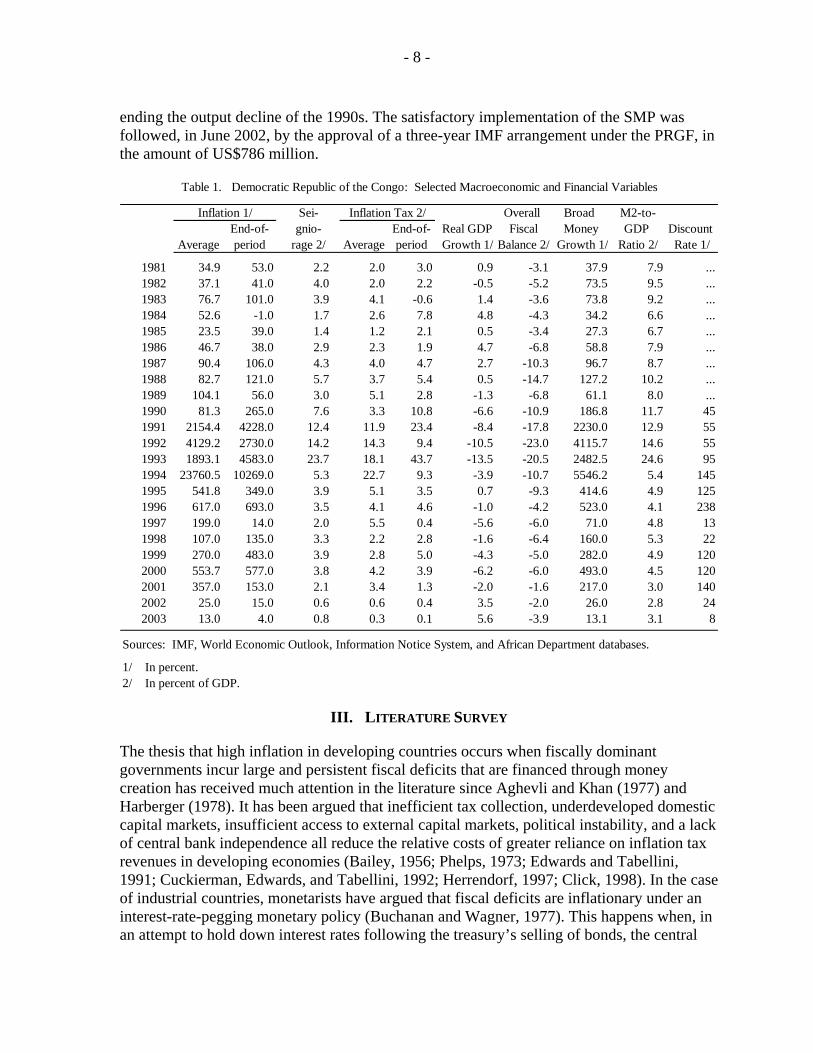
The Mobutu presidency brought relative political stability by reducing the influence of ethnic and regional forces. Between 1965 and 1973, output expanded at an average rate of 5 percent a year, largely because of favorable terms of trade and increased foreign direct investment. During this period, inflation averaged 21 percent a year, and the external current account was in surplus.6 Between 1974 and 1982, the DRC faced adverse terms of trade shocks—the 1974 rise in the price of oil was followed by the 1975 fall in copper prices—which, combined with the disruptions caused by the “zaïrianization” and nationalization of foreign-owned businesses, led to an average output decline of 1.5 percent a year.7 A policy of increased government spending, financed through money creation and heavy external borrowing, caused inflation to jump to an average of 53 percent a year and created current account deficits.8 Selected economic and financial variables for 1981-2003 are given in Table 1.

During 1983–89, the DRC undertook a series of stabilization and adjustment programs supported by the IMF and the World Bank, beginning in 1983 with the free float of the zaïre.9 The results, in terms of the goals of lowering inflation and accelerating growth, were mixed. At first, during 1984–86, the economy responded favorably to reforms, including price and trade liberalization measures: real GDP growth averaged 3.3 percent while inflation (measured on an annual average basis) slowed from 77 percent in 1983 to 24 percent in 1985. 5 Mineral production, the mainstay of the formal economy, remained broadly stable. For instance, copper production in 1965 was estimated at about 262,000 tons, or the same level as in 1959. See Kiakwama and Chevalier (2001).

6 However, the formal introduction of a single-party system in 1972 marked the beginning of continual governance problems.

7 “Zaïrianisation” involved the transfer by the government of foreign-owned economic activities to Zaïrian nationals.

8 On March 12, 1976, the Zairian currency (Z), which had been fixed at a value of Z 0.50 per U.S. dollar since 1967 when it replaced the Congolese franc, was devalued by 46 percent and fixed at par with the SDR. This measure was followed by six more devaluations, bringing the rate to Z 3.95 per SDR by February 1980.

9 In addition, fiscal reform, exchange rate unification, and price and trade liberalization measures were implemented.

- 6 -

But, by late 1986, an increase in public spending derailed the adjustment program, and some of the liberalization measures were reversed. In June 1989, the government made a last effort to stabilize the economy with IMF support. Although inflation fell to 56 percent from over 100 percent in 1988, GDP per capita fell by more than 4 percent.10 Thus, over 1987–89, despite significant external support and export earnings growth, real GDP increased by only 0.6 percent a year while inflation averaged 94 percent a year.

C. The 1990-2000 Period

In the early 1990s, inflation jumped to hyperinflation levels. On April 24, 1990, President Mobutu, under pressure from donors and the political changes stemming from Eastern Europe, announced that the DRC would move from a single-party system to a multiparty democracy.11 Mounting social pressures soon led to an unprecedented relaxation of fiscal policy, particularly affecting salaries and nonwage outlays of the civil service and of political and military institutions. The political turmoil and the tense social climate strained the government’s relations with its traditional external partners; by November 1990, a large part of official bilateral aid to the DRC was suspended or terminated. In addition, in September 1990, the DRC experienced an adverse supply shock, when a cave-in at the Kamoto copper mine belonging to Gécamines (the state-owned mining company) cut output by more than 23 percent in 1990 relative to its 1989 level and led to a drop in budget revenues. The fiscal deficit jumped to 11 percent of GDP in 1990, which the government financed by accumulating domestic and external arrears and by printing money.12 The widening fiscal deficit plunged the country into a vicious cycle of hyperinflation, currency depreciation, and output decline. In 1990, inflation and money growth jumped to 265 percent and 189 percent, respectively, and averaged 5,452 percent and 3,594 percent over 1991–94, as the government lost control over financial policies. In early 1995, the government launched a disinflation program based on fiscal consolidation and credit restraint. This program came under increasing political pressure and was abandoned in the second half of the year. Even so, inflation slowed to 521 percent during 1995-96, as the fiscal deficit was significantly reduced to 6.8 percent of GDP from an average of 19 percent during 1991–94.

In May 1997, after a six-month rebellion, Laurent-Désiré Kabila became president, and the country’s name was changed from Zaïre back to the Democratic Republic of the Congo. Following the adoption of strict fiscal and monetary policies, inflation fell to 14 percent in 1997. In August 1998, a month after a new currency—the Congolese franc—was issued, a new rebellion caused the country to split in half, with the government controlling the south and west and the rebels controlling most of the east and north. In response to the economic 10Unless otherwise indicated, rates of inflation are measured on an end-of-period basis.

11 The transition was supposed to prepare for free presidential and legislative elections at the end of 1991 and during 1992, respectively.

12 Unable to borrow from the domestic private sector or from abroad, and having exhausted its foreign reserves, the government borrowed from the central bank, its only option.

- 7 -

disruptions and financing needs created by this second war, monetary policy became accommodative, and inflation increased to 135 percent in 1998 and to more than 500 percent in 2000.

The degree of FD in the 1990s and 2000 can also be seen in the evolution of seigniorage and the inflation tax.13 Seigniorage and the inflation tax, which averaged 3.2 percent of GDP in 1981-89, jumped to an average of 14.5 percent and 21.8 percent, respectively, in 1990-93. The difference between seigniorage and the inflation tax is a function of the change in the demand for real cash balances, which depends, other things (real income, interest rate, etc.) being equal, on expected inflation. For instance, the rise in inflation in 1994 was not accompanied by an increase in seigniorage for that year, even though the growth rate of M2 more than doubled. This was due to a steep decline in real cash balances in 1994 in an environment of high inflationary expectations and falling real GDP. Also noteworthy was the inefficiency of inflationary financing, as demonstrated by the fact that the cost inflicted on the public—that is, the inflation tax (9.3 percent of GDP) —was much higher than the real resources “collected” by the government—that is, the seigniorage (5.3 percent of GDP). During the 1990s and in 2000 overall, the inflation tax (10.6 percent of GDP) was much higher, on average, than seigniorage (7.6 percent).

D. The 2001-03 Period

On January 16, 2001, President Kabila was assassinated, and his son Joseph Kabila was elevated to the presidency. President Joseph Kabila announced his intention to seek a peaceful end to the civil war, normalize relations with the international community, introduce multiparty democracy, and liberalize the economy. In May 2001, the government negotiated an IMF SMP covering the period June 2001-March 2002 and aimed at restoring macroeconomic stability and laying the foundation for a recovery of economic growth.14 A fiscal policy limiting public expenditure to cash in the treasury account at the Central Bank of Congo (BCC) was implemented, effectively halting excessive money creation. In the monetary area, interest rates were liberalized, liquidity management by the BCC was improved, and the autonomy of the BCC was restored. In addition, on May 26, 2001, the Congolese franc, which had appreciated in real effective terms by about 45 percent since November 2000, was devalued by more than 527 percent vis-à-vis the U.S. dollar (in national currency terms). A free floating exchange rate regime was reestablished, and the foreign exchange market was unified. Last, urgent structural reforms were implemented, notably the liberalization of diamond export activities, transportation tariffs, and the prices of petroleum products. The results were encouraging: inflation (money supply growth) slowed sharply, from 153 (217) percent in 2001 to a yearly average of 10 (19.5) percent over 2002-03, while real GDP growth increased from -2 percent to 4.4 percent over the same period, effectively

13 The inflation tax refers to the cost inflicted on the private sector’s existing stock of money balances as a result of inflation. See Section IV.

14 See, for instance, Matungulu (2003), Clément (2004), and Masangu (2004).

- 8 -

ending the output decline of the 1990s. The satisfactory implementation of the SMP was followed, in June 2002, by the approval of a three-year IMF arrangement under the PRGF, in the amount of US$786 million.

Sei- Overall Broad M2-to-End-of- gnio- End-of- Real GDP Fiscal Money GDP Discount

Average period rage 2/ Average period Growth 1/ Balance 2/ Growth 1/ Ratio 2/ Rate 1/

1981 34.9 53.0 2.2 2.0 3.0 0.9 -3.1 37.9 7.9 ...1982 37.1 41.0 4.0 2.0 2.2 -0.5 -5.2 73.5 9.5 ...1983 76.7 101.0 3.9 4.1 -0.6 1.4 -3.6 73.8 9.2 ...1984 52.6 -1.0 1.7 2.6 7.8 4.8 -4.3 34.2 6.6 ...1985 23.5 39.0 1.4 1.2 2.1 0.5 -3.4 27.3 6.7 ...1986 46.7 38.0 2.9 2.3 1.9 4.7 -6.8 58.8 7.9 ...1987 90.4 106.0 4.3 4.0 4.7 2.7 -10.3 96.7 8.7 ...1988 82.7 121.0 5.7 3.7 5.4 0.5 -14.7 127.2 10.2 ...1989 104.1 56.0 3.0 5.1 2.8 -1.3 -6.8 61.1 8.0 ...1990 81.3 265.0 7.6 3.3 10.8 -6.6 -10.9 186.8 11.7 451991 2154.4 4228.0 12.4 11.9 23.4 -8.4 -17.8 2230.0 12.9 551992 4129.2 2730.0 14.2 14.3 9.4 -10.5 -23.0 4115.7 14.6 551993 1893.1 4583.0 23.7 18.1 43.7 -13.5 -20.5 2482.5 24.6 951994 23760.5 10269.0 5.3 22.7 9.3 -3.9 -10.7 5546.2 5.4 1451995 541.8 349.0 3.9 5.1 3.5 0.7 -9.3 414.6 4.9 1251996 617.0 693.0 3.5 4.1 4.6 -1.0 -4.2 523.0 4.1 2381997 199.0 14.0 2.0 5.5 0.4 -5.6 -6.0 71.0 4.8 131998 107.0 135.0 3.3 2.2 2.8 -1.6 -6.4 160.0 5.3 221999 270.0 483.0 3.9 2.8 5.0 -4.3 -5.0 282.0 4.9 1202000 553.7 577.0 3.8 4.2 3.9 -6.2 -6.0 493.0 4.5 1202001 357.0 153.0 2.1 3.4 1.3 -2.0 -1.6 217.0 3.0 1402002 25.0 15.0 0.6 0.6 0.4 3.5 -2.0 26.0 2.8 242003 13.0 4.0 0.8 0.3 0.1 5.6 -3.9 13.1 3.1 8

Sources: IMF, World Economic Outlook, Information Notice System, and African Department databases.

1/ In percent.2/ In percent of GDP.

Inflation 1/ Inflation Tax 2/

Table 1. Democratic Republic of the Congo: Selected Macroeconomic and Financial Variables

III. LITERATURE SURVEY

The thesis that high inflation in developing countries occurs when fiscally dominant governments incur large and persistent fiscal deficits that are financed through money creation has received much attention in the literature since Aghevli and Khan (1977) and Harberger (1978). It has been argued that inefficient tax collection, underdeveloped domestic capital markets, insufficient access to external capital markets, political instability, and a lack of central bank independence all reduce the relative costs of greater reliance on inflation tax revenues in developing economies (Bailey, 1956; Phelps, 1973; Edwards and Tabellini, 1991; Cuckierman, Edwards, and Tabellini, 1992; Herrendorf, 1997; Click, 1998). In the case of industrial countries, monetarists have argued that fiscal deficits are inflationary under an interest-rate-pegging monetary policy (Buchanan and Wagner, 1977). This happens when, in an attempt to hold down interest rates following the treasury’s selling of bonds, the central

- 9 -

bank purchases bonds (and thereby increases high-powered money, the money supply, and prices). Sargent and Wallace (1981) formalize the FD hypothesis in a dynamic framework that takes into account the government’s intertemporal budget constraint. They show that if the path of expenditure and revenue is exogenous, then in the long run bond-financing of deficits leads to higher inflation than monetary financing. The tighter monetary policy is in the short run, the higher will be the steady-state rate of inflation, because increased debt will require a greater amount of seigniorage. Thus, under FD, inflation is a fiscally driven monetary phenomenon. A competing fiscal explanation of inflation is provided by the fiscal theory of the price level (FTPL), which argues that bond-financed deficits lead to higher equilibrium prices through their effects on private sector wealth and aggregate demand, whereas money plays no role (Woodford, 1995).15

The empirical evidence of statistically significant links among fiscal deficits, money, and inflation has been mixed, with studies of both industrial and developing countries yielding inconclusive results. Blanchard and Fischer (1989, p. 513) note that “a common criticism of this stress on the budget deficit is that the data rarely show a strong positive association between the size of the budget deficit and the rate of inflation.” Most of the early studies on industrial countries were focused on the United States. Barro (1977, 1978a, b), Niskanen (1978), Dwyer (1982), and Joines (1985) find insignificant results, while Levy (1981), Barth, Sickles and Wiest (1983), and Laney and Willet (1983) find significant monetization of all or most of the deficits.16 Hamburger and Zwick (1981), Allen and Smith (1983), Ahking and Miller (1985), and Grier and Neiman (1987) find that the deficit-money linkage is not invariant to the sample period covered, while Giannaros and Kolluri (1985) and King and Plosser (1985) argue that, except for the United States, there is no general evidence of a deficit-money growth link in industrial countries.17 18 In developing countries, Dornbusch and Fischer (1981) and De Haan and Zelhorst (1990) find that the link between deficits and monetary growth is not strong, while Edwards and Tabellini (1991) find fiscal deficits to be

15 The FTPL does not rule out a positive correlation between money and prices, but argues that causality runs from the fiscal deficit to prices and from prices to money.

16 Barro and Joines find that money growth is related to war spending but not to nonwar deficits. Niskanen finds that deficits do not affect inflation, directly or indirectly, through money growth.

17 Hamburger and Zwick confirm Barro’s findings that in the United States over 1954-76 it was government expenditure rather than deficits that influenced money growth. Over the longer 1961-82 period, however, deficits have a stronger effect on money growth than spending. McMillin and Beard (1982) reexamined Hamburger and Zwick findings (using revised national accounts data) and could not find any deficit-money linkage.

18 Ahking and Miller use a trivariate autoregressive process and find that deficits were inflationary in the 1950s and 1970s, directly and independently of their effects on money growth. In the 1960s, however, both inflation and deficits were exogenous to money.

- 10 -

inflationary in 21 countries. Montiel (1989) and Dornbusch, Sturzenegger, and Wolf (1990) use a sample of high-inflation countries and conclude that deficits and money growth are driven by, and do not drive, inflation. Click (1998) uses a cross-section of 90 (mostly developing) countries and finds that 40 percent of the cross-country variation of seigniorage is explained by the optimum tax theory, with transitory government spending, central bank independence, and political instability accounting for the remaining variation.

Recent studies by Fischer, Sahay, and Végh (2003) and Catao and Terrones (2005) used panel data methods on a large sample of countries, and found a significant relationship between deficits and inflation, with the statistical evidence much stronger in the case of high- inflation (developing) countries than in low-inflation (industrial) countries. Recent studies of individual countries, using multivariate cointegration and error-correction modeling, have also established significant relationships among deficits, money growth, and inflation. Metin (1998) uses annual data for Turkey over 1950-87 and finds that deficits and debt monetization are inflationary. Tekin-Koru and Ozmen (2003) challenge these findings and show that although deficits are exogenous to money (M2) growth in Turkey, the relationship between inflation and money growth is bidirectional. Darrat (2000) indicates that in Greece, both deficits and money growth are inflationary, a result that is consistent with both the FD hypothesis and the FTPL. Sowa (1994) finds that output variability is more inflationary than monetary factors in Ghana, while Ghartey (2001) presents strong evidence of FD in Ghana. Favero and Spinelli (1999) find empirical support for the FD hypothesis in Italy over 1875-1975. They show, however, that relationships among deficits, money growth, and inflation may not be invariant to a policy shift toward central bank independence.19

IV. THEORY, METHODOLOGY, AND DATA

Since the DRC went from high inflation in the 1980s to hyperinflation in the 1990s, we will begin by discussing briefly the factors and conditions that are important in the emergence and dynamics of hyperinflation. Cagan (1956), whose classic work is the starting point of most studies of extreme inflation, defined hyperinflation “as beginning in the month the rise in prices exceeds 50 percent (12,875 percent yearly) and as ending in the month before the monthly rise in prices drops below that amount and stays below for at least a year.” Although useful in his study of cases of extreme inflation in Europe (Austria, Germany, Hungary, Poland, and Russia) following World War I, Cagan's threshold for defining hyperinflation is arbitrary. Modern economic literature places greater emphasis on the following—mostly qualitative—characteristics of high or hyperinflation periods: (1) a decrease in real cash balances and an increase in velocity; (2) a process of currency substitution coupled with rapid depreciation of the exchange rate; (3) fiscal chaos caused by the erosion of real tax revenue, stemming from the acceleration of inflation and lags in tax collection (the “Keynes-Olivera-

19A structural break emerges between deficits and money growth once their model is applied to the 1975-94 period. Lack of central bank independence began to be perceived as a serious problem in 1975. The independence of the Bank of Italy was ratified in 1981.

- 11 -

Tanzi effect”);20 and (4) explosive and unstable changes in the inflation rate, causing distortions in relative prices (the real exchange rate, interest rate, and wages), malfunctions in various markets, and a decline in economic activity.

There is general agreement about the causes of high inflation or hyperinflation. Its main cause is the systematic financing of large budget deficits through seigniorage (SEI), defined as real revenues collected by the government by virtue of its monopoly on the printing of money (SEI = ∆M/P). When the government forces private agents to hold an additional stock of money on which it pays no interest, it collects, as a result of inflation (INF), an implicit tax on the existing real money holdings (Mt-1/P), called the inflation tax (IT).21 The inflation tax base is made up of real base money (currency and commercial banks' reserves) and depends on the growth rate of real income and the elasticity of the demand for real cash balances with respect to inflation and real income. Assuming unitary income elasticity of the real demand for money, the inflation tax may be described as the product of the inflation rate and real base money: INF* Mt-1/P.

The monetization of a series of large budget deficits, even if they are constant in real terms, is potentially hyperinflationary because, at current price levels, monetization continuously places excess cash balances in the hands of the public. The increase in inflationary expecta-tions (that is, the anticipation of an increased opportunity cost of holding money) is reflected in a falling demand for real cash balances, as the public makes costly efforts to minimize its local currency holdings, either by seeking more stable assets (for example, foreign curren-cies) or by turning to barter arrangements. Beyond the optimal inflation rate—the rate that maximizes the revenues from seigniorage and at which the elasticity of real money demand to the expected inflation rate equals one (Cagan, 1956)22 —the process becomes unstable. The position is then to the right of the Laffer curve, where any increase in the inflation rate produces a stronger decline in real cash balances, which have become extremely sensitive to changes in the expected inflation rate. The fall in real money demand also reduces the real value of the money that the government is printing. Where real government expenditures remain unchanged, desperate attempts to increase the rate of monetary growth to offset the decline in seigniorage revenues will lead to hyperinflation. The relationship between the budget deficit and inflation is intensified by the Keynes-Olivera-Tanzi effect, because the high rate of inflation in turn increases the real fiscal deficit (and therefore the rate of

20 See Keynes (1923), Olivera (1967), and Tanzi (1977).

21 See Bailey (1956) for an early analysis of the welfare cost of inflation.

22Assuming a zero growth rate for real income. See Friedman (1971).

- 12 -

monetary expansion).23 This implies that both the money supply and the budget deficit are potentially endogenous to the inflationary process.24

The basic model underpinning the preceding discussion can be summarized as follows:

INF = f (DEFY, X) , (1)

where INF is the rate of inflation, DEFY is the overall fiscal deficit in percent of GDP, and X is a vector of potential conditioning variables: income velocity (VELO), real GDP growth (GRY), seigniorage in percent of GDP (SEIY), broad money growth (GRM), and currency depreciation (GREX). Note that although we expect the conditioning variables to be weakly exogenous with respect to inflation, there is no reason (a priori) to assume this. The function f is assumed to be increasing in DEFY, SEIY, VELO, GREX, and GRM and decreasing in GRY. The FD hypothesis implies that DEFY affects INF through its effect on GRM or SEIY: GRM and SEIY are weakly exogenous to INF. A direct and independent relationship between DEFY and INF, while controlling for monetary policy impact (SEIY or GRM), may indicate some kind of FTPL relationship. Increases in GRY will reduce inflation directly, through a larger supply of goods, or indirectly, through higher transactions money demand, or both.25 VELO is expected to influence INF positively because it captures the impact of the loss of confidence in the national currency, resulting from expectations of a higher inflation or currency depreciation. For a given level of the fiscal deficit, the higher the expected rate of inflation or currency depreciation, the higher the flight out of money (and the lower the demand for money), and the higher will be the equilibrium rate of inflation.26 Figure 1 plots the series that are used to test the FD hypothesis in the DRC. All the series are annual and are taken from the IMF’s World Economic Outlook and Information Notice System databases. See Appendix I for the definitions and construction of the variables.

Equation (1), however, assumes an instantaneous adjustment of actual inflation to its equilibrium level given its determinants. Instantaneous adjustment is unlikely, given the 23 See Dornbusch, Sturznegger, and Wolf (1990) for a model of interaction between inflation and the real fiscal deficit.

24 There is, however, another important factor driving the strong growth of base money during periods of extreme inflation: the granting of credit to the private sector. This essentially consists of advances intended to enable enterprises to meet their obligations resulting from the indexation of money wages. It may be judged politically unsustainable for the monetary authorities to refuse for very long to implement an accommodative monetary policy in this respect, given the erosion of real wages and the resulting social conflicts.

25For a given money stock, the equilibrium in the money market is restored through reductions in actual prices or lower inflation. See, for instance, Aghevli and Khan (1977).

26Assuming a unitary income elasticity of real money demand, velocity will depend solely on the expected opportunity cost of holding money.

- 13 -

effects of transaction costs and uncertainty on the speed of adjustment in the money market, where inflation is ultimately determined.27 In addition, the equilibrium level of inflation is unobservable. A distinction is therefore made between the long- and short-run behaviors of inflation, by specifying an error-correction mechanism of actual inflation toward its long-run level. Furthermore, the above econometric time series have stochastic trends, and various subsets of these could be cointegrated. Therefore, our empirical implementation will proceed in three steps. First, the time-series properties of the data are investigated to avoid the spurious regression problem that arises when statistical inferences are drawn from nonstationary time series. Second, the Johansen (1988) and Johansen and Juselius (1990) multivariate cointegration procedures are used to determine empirically the number of cointegrating vectors, the values of the adjustment parameters, and the exogeneity status of each variable included in the model. Third, simultaneous equations systems—the full-information maximum likelihood procedure—are used to estimate parsimonious SVECMs of inflation and money creation.

V. ECONOMETRIC RESULTS

A. Unit-Root Tests

We investigate the integrating properties of the variables by conducting unit-root tests, namely, the augmented Dickey-Fuller (ADF) tests (Table 2). The null hypothesis is the presence of a unit root. The lag length in the ADF regression is selected using the Akaike information criterion. The ADF tests are performed by including both a constant and a deterministic time trend. With the exception of GREX, all series are found to be unequivocally nonstationary; that is, the null hypothesis that they contain a unit root could not be rejected at the 5 percent critical value or less. Once expressed in first differences, all the series turn out to be stationary. Hence, all the series considered here are integrated of order one (or I (1)). The stationarity of currency depreciation implies that the series can be excluded from the cointegration analysis (without loss of generality) and, later, included in the vector error-correction model capturing the short-run dynamics.

B. Fiscal Deficits, Seigniorage, and Inflation

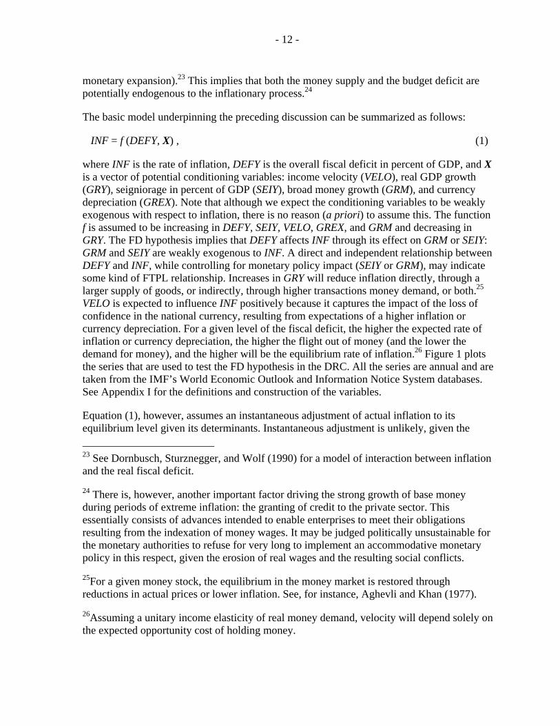
After determining the order of integration of the variables, the Johansen procedure is first applied to a first-order vector autoregression (VAR) simplified version of equation (1) to test for cointegration among the fiscal deficit, inflation, output growth, and seigniorage.28 The maximal and trace eigenvalue statistics reject the null hypothesis of no cointegrating vector in favor of two cointegrating vectors at the 5 and 10 percent levels, respectively (see Table 3). The two cointegrating vectors are not uniquely determined in terms of stationarity, 27 Note that since we are testing the FD hypothesis, we implicitly assume that inflation is determined in the money market.

28 Throughout this paper, the optimal lag length of the VAR is chosen on the basis of the Schwarz-Bayesian criterion. Also, all models tested for cointegration contain a constant term.

- 14 -

because any linear combination of them is also stationary. System identification implies that the fiscal deficit should be excluded from the first cointegrating vector and that inflation should be excluded from the second one.

1980 1985 1990 1995 2000

0

5000

10000

Figure 1. Macroeconomic and Financial Variables

Inflation

1980 1985 1990 1995 2000

2500

5000M2 growth rate

1980 1985 1990 1995 2000

-10

0

Real GDP growth

1980 1985 1990 1995 2000

10

20

30

40Broad money velocity

1980 1985 1990 1995 2000

10

20Seignioriage (in percent of GDP)

1980 1985 1990 1995 2000

10

20Fiscal deficit (in percent of GDP)

After imposing (over) identifying restrictions (normalizing the first and second vectors on INF and SEIY, respectively; testing for the weak exogeneity of SEIY, GRY, and DEFY in the first vector and of DEFY and ΙΝF in the second vector; and testing for significance of GRY in the second vector), the following long-run relationships cannot be rejected by the data-generating process:

INF = 409.90 SEIY - 15.30 GRY (2)

and

SEIY = 0.81 DEFY , (3)

where estimated constants and random error terms are omitted for brevity. The restrictions on the beta and alpha coefficients result in a likelihood ratio (LR) test statistic of 10.9, which is asymptotically distributed as χ2

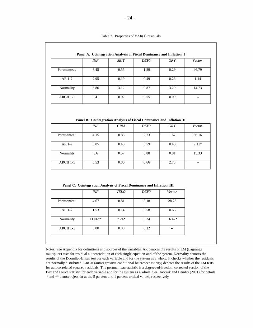
(6) and insignificant. The first restricted vector links inflation to seigniorage and output growth, while the second one links seigniorage to the fiscal deficit. Various misspecification tests of the unrestricted VAR (1) underlying the system of equations (2)-(3) are reported in Table 7. These include single-equation tests (normality, AR, ARCH, and portmanteau), and vector tests (normality, AR, and portmanteau). Neither the single-equation nor the vector tests reveal any problem.

- 15 -

1980 1985 1990 1995 20000

5000

10000Figure 1. Macroeconomic and Financial Variables (concluded)

Inflation Seigniorage (in percent of GDP )

1980 1985 1990 1995 2000

10

20Seigniorage (in percent of GDP ) Fiscal deficit (in percent of GDP )

1980 1985 1990 1995 2000

0

2500

5000Rate of growth of M2 Fiscal deficit (in percent of GDP )

1980 1985 1990 1995 20000

5000

10000Inflation Rate of growth of M2

1980 1985 1990 1995 2000

0

10

20The negative of real GDP growth Rate of growth of M2

1980 1985 1990 1995 20000

5000

10000 Inflation Rate of change of exchange rate

- 16 -

Table 2. ADF (3) Statistics for Testing for a Unit Root

Variables t-adf Lag Additional regressors

In levelsINF -2.64 0 Constant and trendGRM -2.38 0 Constant and trendDEFY -2.33 0 Constant and trendVELO -2.36 1 Constant and trendGRY -1.42 0 Constant and trendSEIY -2.33 0 Constant and trendGREX -3.93* 0 Constant and trend

In first differencesINF -6.28** 0 Constant and trendGRM -6.68** 0 Constant and trendDEFY -3.87* 0 Constant and trendVELO -4.10* 0 Constant and trendGRY -4.19* 0 Constant and trendSEIY -5.39** 0 Constant and trendGREX -6.64** 0 Constant and trend

Notes: The estimation period is 1986-2003. For each variable, the t value of the augmented Dickey-Fuller (ADF) statistics, with critical values based on the response surface in MacKinnon (1991). Lag denotes its lag order.For each variable expressed in level (first difference), the ADF(3) statistics are testing a null hypothesis of aunit root in that variable expressed in level (first difference) against an alternative of a stationary root. Here and elsewhere in this paper, * and ** denote rejection at the 5 percent and 1 percent critical values. The Johansen approach provides a systems approach for testing the existence of unit roots in each variable when the null hypothesis is that of stationarity rather than nonstationarity. The various chi-square statistics reported in Table 3 confirm that all the variables considered here are indeed nonstationary, and, with the exception of GRY, the estimated coefficients are significantly different from zero. Furthermore, the weak exogeneity of inflation (in the first vector) and fiscal deficits (in the second vector) were rejected, suggesting that inflation and seigniorage adjust, respectively, to seigniorage and the fiscal deficit, but the converse is not true: χ2

(1) =52.6[0.00] and χ2(1) =11.4[0.00], respectively.29 30

The estimated adjustment parameters in both vectors are negative and just equal to unity, suggesting that (short-run) deviations from these long-run equilibrium relationships are fully corrected within a year. All the coefficients in the system of equations (2)-(3) have the expected signs. However, the coefficient of GRY in equation (2) is not statistically 29 This amounts to imposing zero restrictions on the feedback parameters of SEIY and DEFY, respectively, in the first and second vectors.

30 Throughout this paper, asymptotic p-values are presented in square brackets following the observed chi-square statistics.

- 17 -

significantly different from zero (χ2(1) = 0.52047[0.4706]). Under such a hypothesis, the

coefficient of SEIY increases to 422.14, suggesting that a 1 percentage point increase in the seigniorage-to-GDP ratio has been inducing, on average, an increase of about 422 percentage points in the rate of inflation (χ2

(7) = 10.995 [0.1388]). The nonsignificance and nonrejection of the weak exogeneity of GRY with respect to INF suggest that, during the sample period, output growth (or supply shocks) did not affect inflation directly, in either the long or the short run.

Equation (3) tells us that movements in seigniorage revenue were driven by the need to finance the real fiscal deficit and that, on average, more than 80 percent of the nominal (real) fiscal deficit was financed through money creation (seigniorage revenue).31 GRY does not appear in equation (3) because, after identification of the beta matrix, its coefficient is not statistically significantly different from zero: χ2

(1) = 1.83 [0.1756]. Under such an assumption, the weak exogeneity of GRY with respect to SEIY is rejected (χ2

(2) = 10.83 [0.0045]), suggesting that output growth affects seigniorage revenue in the short run but not in the long run. The feedback coefficient of GRY in the second vector is positive and equals to 0.57. Thus, a negative (positive) short-run disequilibrium in relation (3), such that actual seigniorage is lower (higher) than the financing needs of the government, leads to an increase (decrease) in output growth. This in turn induces higher (lower) real money demand or, equivalently, lower (higher) velocity, and hence higher (lower) seigniorage revenue.32 The system reverts to its long-run equilibrium through this adjustment mechanism. Thus, output growth has been affecting inflation in the short run and only indirectly through its effect on the demand for money. In turn, money demand plays an indirect role in the short-run adjustment mechanism of inflation by determining the amount of seigniorage revenue that the government is able to collect through money creation. Finally, the thesis that higher (lower) output growth affects positively (negatively) seigniorage revenue through lower (higher) broad money velocity implies an income elasticity of money demand that is significantly higher than unity.33 The thesis of no long-run presence of velocity as a determinant of inflation is addressed below.

31 Since both the left- and right-hand variables are divided by nominal GDP, equation (3) also relates the nominal fiscal deficit to the (absolute) change in the money stock.

32 Recall that seigniorage revenue is measured as the absolute change in M2 in percent of GDP, or 100*( Mt - Mt-1)/GDP, which is equivalent to the product of GRM and Mt-1 / GDP. GRM is the growth rate of M2 while Mt-1/GDP is an approximate measure of inverse velocity or, equivalently, of the demand for money. Formally, GRM = 100 * (Mt - Mt-1) / Mt-1.

33 Nachega (2005) estimates the income elasticity of money demand at 1.5 over 1981-2003.

- 18 -

Table 3. Cointegration Analysis of Fiscal Dominance and Inflation I

Eigenvalues 0.94 0.68 0.25 0.15Hypotheses r = 0 r <= 1 r <= 2 r <= 3Lambda max 54.38** 21.41* 5.44 3.01Lambda trace 84.23** 29.86* 8.45 3.01

Unrestricted system Standardized eigenvectorsINF SEIY DEFY GRY

First vector 1.00 -518.36 93.36 10.71Second vector 0.03 1.00 -32.18 4.63

Standardized adjustment coefficients INF SEIY DEFY GRY

First vector -1.08 0.00 0.00 0.00Second vector 0.19 0.00 0.01 0.00

Identified system Standardized eigenvectorsINF SEIY DEFY GRY

First vector 1.00 -374.80 0.00 37.01Second vector 0.00 1.00 -0.65 0.18

Standardized adjustment coefficients INF SEIY DEFY GRY

First vector -1.09 0.00 0.00 0.00Second vector 128.25 -1.57 -0.26 0.88

Overidentified system Standardized eigenvectorsINF SEIY DEFY GRY

First vector 1.00 -409.90 0.00 15.30Second vector 0.00 1.00 -0.81 0.00

Standardized adjustment coefficients INF SEIY DEFY GRY

First vector -1.15 0.00 0.00 0.00Second vector 0.00 -1.10 0.00 0.57

Weak exogeneity test statistics: χ2(1)INF SEIY DEFY GRY

First vector 52.6** 0.6 0.2 1.9Second vector 2.9 11.4** 0.4 5.7**

Multivariate statistics for testing stationarity: χ2(2)INF SEIY DEFY GRY

19.1** 20.7** 21.8** 21.1**

Notes: The estimation period is 1981-2003. See appendix for definitions and sourcesof variables. The VAR includes one lag on each variable and a constant term. Johansen's maximal and trace eigenvalue statistics for testing cointegration areadjusted for degrees of freedom. The systems-based test statistics for weak exogeneity and stationarity are evaluated under the assumption that r =2 and, hence, are assymptotically distributed as χ2(1) or χ2(2) if weak exogeneity or stationarity of the specified variable is accepted.

- 19 -

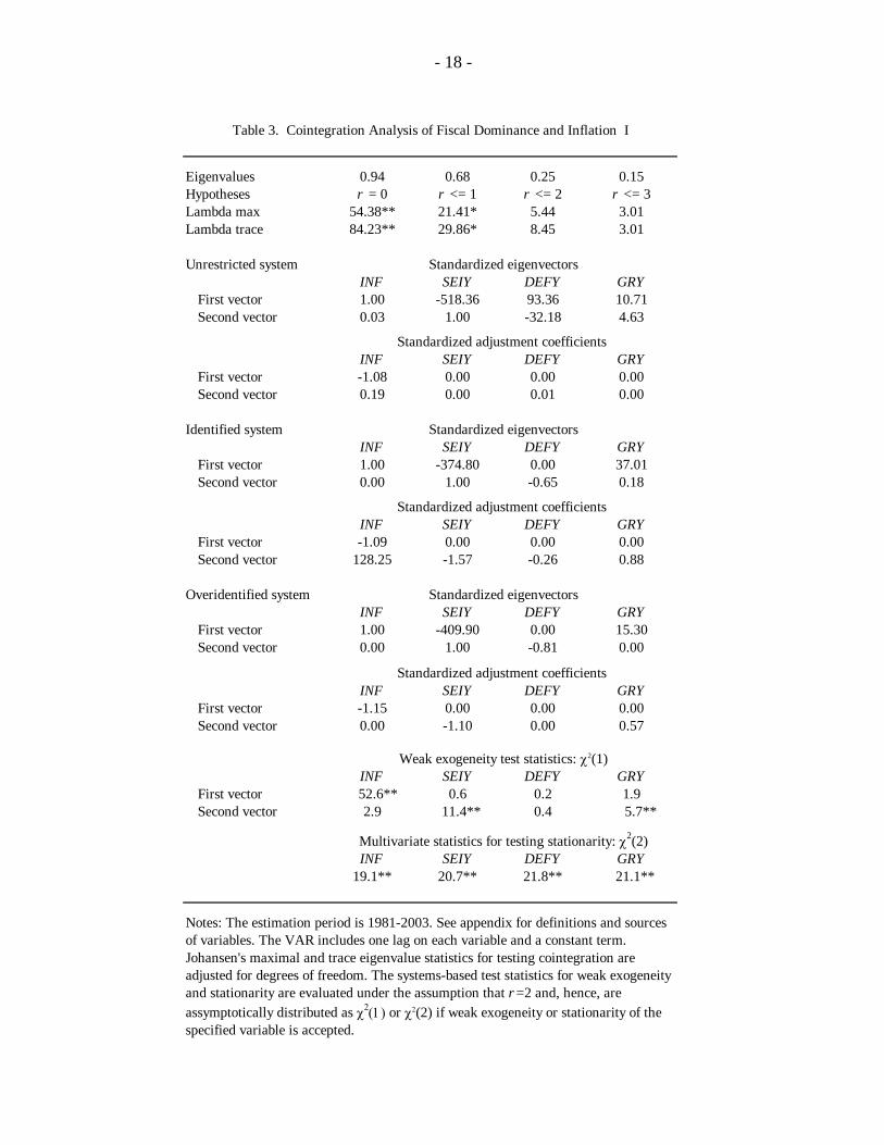
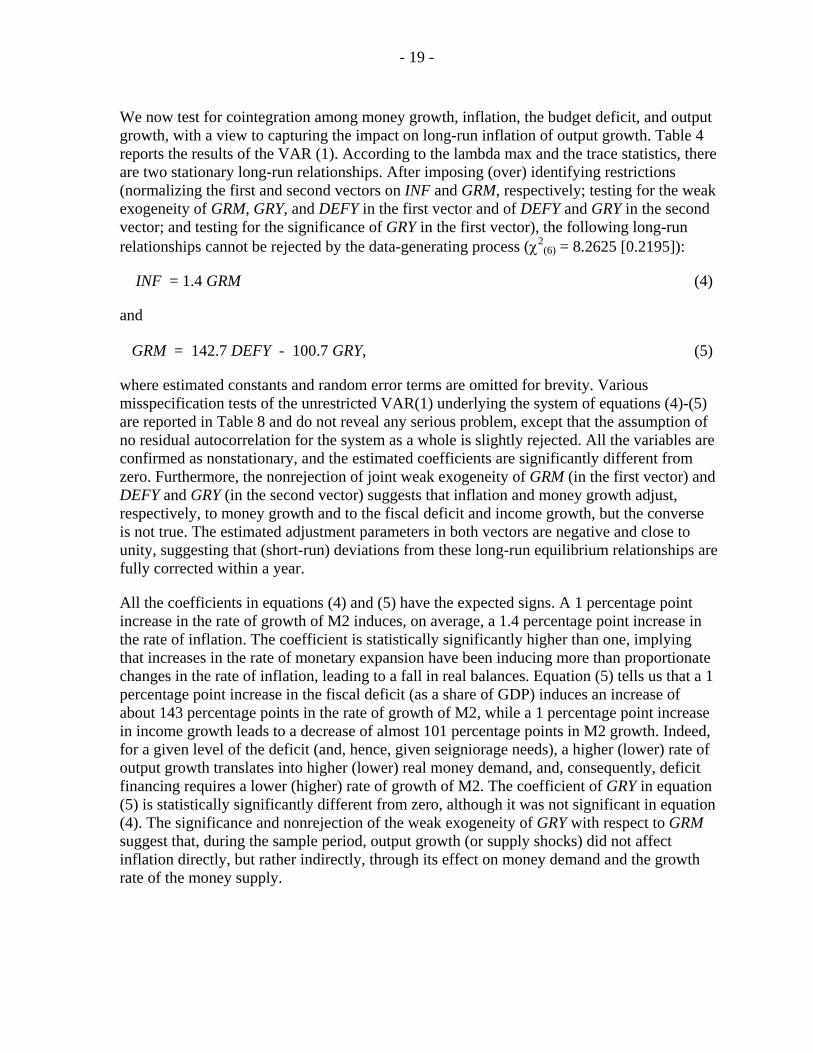
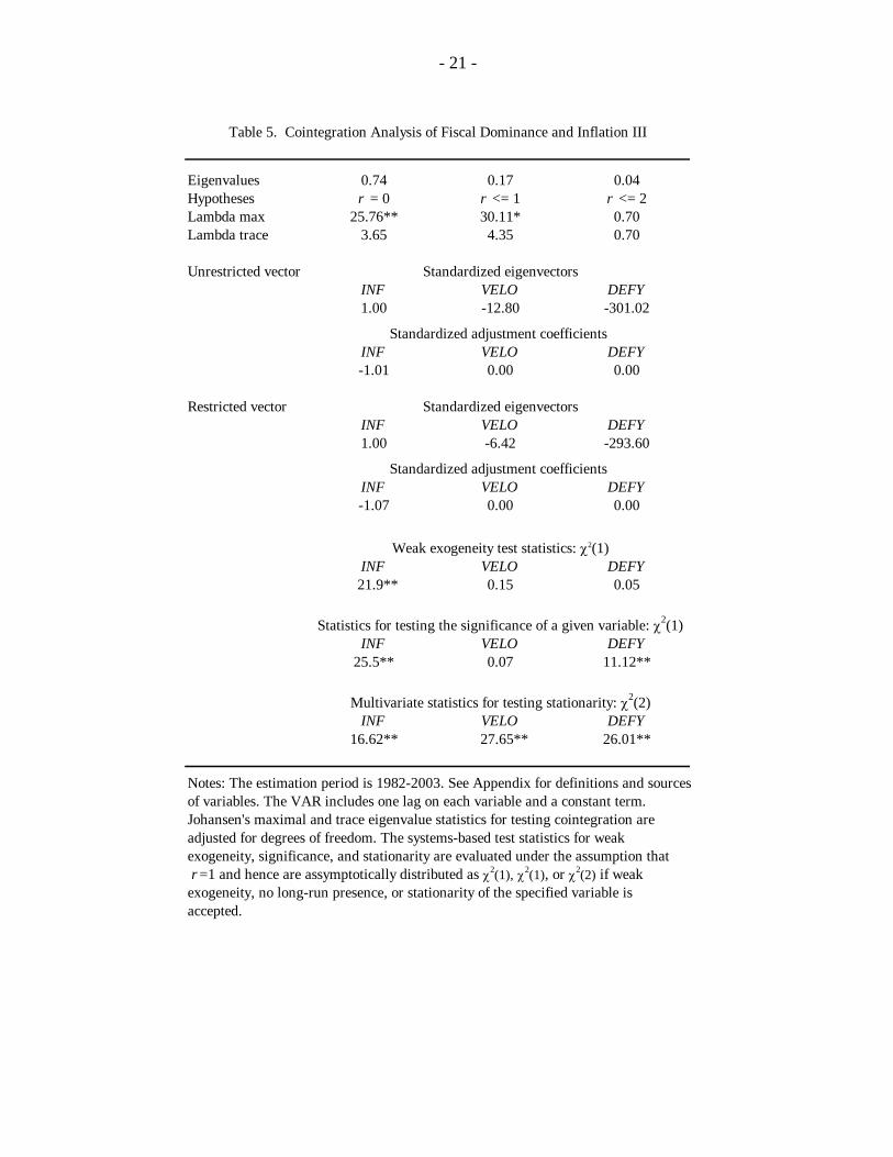
We now test for cointegration among money growth, inflation, the budget deficit, and output growth, with a view to capturing the impact on long-run inflation of output growth. Table 4 reports the results of the VAR (1). According to the lambda max and the trace statistics, there are two stationary long-run relationships. After imposing (over) identifying restrictions (normalizing the first and second vectors on INF and GRM, respectively; testing for the weak exogeneity of GRM, GRY, and DEFY in the first vector and of DEFY and GRY in the second vector; and testing for the significance of GRY in the first vector), the following long-run relationships cannot be rejected by the data-generating process (χ2

(6) = 8.2625 [0.2195]):

INF = 1.4 GRM (4)

and

GRM = 142.7 DEFY - 100.7 GRY, (5)

where estimated constants and random error terms are omitted for brevity. Various misspecification tests of the unrestricted VAR(1) underlying the system of equations (4)-(5) are reported in Table 8 and do not reveal any serious problem, except that the assumption of no residual autocorrelation for the system as a whole is slightly rejected. All the variables are confirmed as nonstationary, and the estimated coefficients are significantly different from zero. Furthermore, the nonrejection of joint weak exogeneity of GRM (in the first vector) and DEFY and GRY (in the second vector) suggests that inflation and money growth adjust, respectively, to money growth and to the fiscal deficit and income growth, but the converse is not true. The estimated adjustment parameters in both vectors are negative and close to unity, suggesting that (short-run) deviations from these long-run equilibrium relationships are fully corrected within a year.

All the coefficients in equations (4) and (5) have the expected signs. A 1 percentage point increase in the rate of growth of M2 induces, on average, a 1.4 percentage point increase in the rate of inflation. The coefficient is statistically significantly higher than one, implying that increases in the rate of monetary expansion have been inducing more than proportionate changes in the rate of inflation, leading to a fall in real balances. Equation (5) tells us that a 1 percentage point increase in the fiscal deficit (as a share of GDP) induces an increase of about 143 percentage points in the rate of growth of M2, while a 1 percentage point increase in income growth leads to a decrease of almost 101 percentage points in M2 growth. Indeed, for a given level of the deficit (and, hence, given seigniorage needs), a higher (lower) rate of output growth translates into higher (lower) real money demand, and, consequently, deficit financing requires a lower (higher) rate of growth of M2. The coefficient of GRY in equation (5) is statistically significantly different from zero, although it was not significant in equation (4). The significance and nonrejection of the weak exogeneity of GRY with respect to GRM suggest that, during the sample period, output growth (or supply shocks) did not affect inflation directly, but rather indirectly, through its effect on money demand and the growth rate of the money supply.

- 20 -

Table 4. Cointegration Analysis of Fiscal Dominance and Inflation II

Eigenvalues 0.81 0.75 0.26 0.14Hypotheses r = 0 r <= 1 r <= 2 r <= 3Lambda max 31.91** 26.50** 5.58 2.42Lambda trace 67.03** 35.12* 8.01 2.42

Unrestricted system Standardized eigenvectorsINF GRM DEFY GRY

First vector 1.00 -4.84 492.71 -352.78Second vector -0.67 1.00 5.99 24.56

Standardized adjustment coefficients INF GRM DEFY GRY

First vector 0.55 0.36 0.00 0.00Second vector 1.75 -0.06 0.00 0.00

Identified system Standardized eigenvectorsINF GRM DEFY GRY

First vector 1.00 -1.55 0.00 -42.35Second vector 0.00 1.00 -149.67 94.30

Standardized adjustment coefficients INF GRM DEFY GRY

First vector -0.61 0.40 0.00 0.00Second vector -1.89 -1.17 0.00 0.00

Overidentified system Standardized eigenvectorsINF GRM DEFY GRY

First vector 1.00 -1.42 0.00 0.00Second vector 0.00 1.00 -142.74 100.72

Standardized adjustment coefficients INF GRM DEFY GRY

First vector -1.41 0.00 0.00 0.00Second vector -1.70 -1.18 0.00 0.00

Multivariate statistics for testing stationarity: χ2(2)INF GRM DEFY GRY

21.0** 27.5** 28.1** 27.6**

Notes: The estimation period is 1981-2003. See appendix for definitions and sourcesof variables. The VAR includes one lag on each variable and a constant term. Johansen's maximal and trace eigenvalue statistics for testing cointegration areadjusted for degrees of freedom. The systems-based test statistics for stationarity are evaluated under the assumption that r =2 and, hence, are assymptoticallydistributed as χ2(2) if stationarity of the specified variable is accepted.

- 21 -

Table 5. Cointegration Analysis of Fiscal Dominance and Inflation III

Eigenvalues 0.74 0.17 0.04Hypotheses r = 0 r <= 1 r <= 2Lambda max 25.76** 30.11* 0.70Lambda trace 3.65 4.35 0.70

Unrestricted vector Standardized eigenvectorsINF VELO DEFY1.00 -12.80 -301.02

Standardized adjustment coefficients INF VELO DEFY-1.01 0.00 0.00

Restricted vector Standardized eigenvectorsINF VELO DEFY1.00 -6.42 -293.60

Standardized adjustment coefficients INF VELO DEFY-1.07 0.00 0.00

Weak exogeneity test statistics: χ2(1)INF VELO DEFY

21.9** 0.15 0.05

INF VELO DEFY25.5** 0.07 11.12**

Multivariate statistics for testing stationarity: χ2(2)INF VELO DEFY

16.62** 27.65** 26.01**

Notes: The estimation period is 1982-2003. See Appendix for definitions and sources of variables. The VAR includes one lag on each variable and a constant term. Johansen's maximal and trace eigenvalue statistics for testing cointegration areadjusted for degrees of freedom. The systems-based test statistics for weakexogeneity, significance, and stationarity are evaluated under the assumption that r =1 and hence are assymptotically distributed as χ2(1), χ2(1), or χ2(2) if weak exogeneity, no long-run presence, or stationarity of the specified variable is accepted.

Statistics for testing the significance of a given variable: χ2(1)

- 22 -

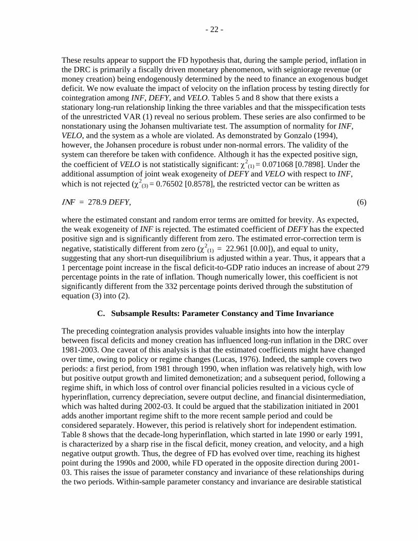
These results appear to support the FD hypothesis that, during the sample period, inflation in the DRC is primarily a fiscally driven monetary phenomenon, with seigniorage revenue (or money creation) being endogenously determined by the need to finance an exogenous budget deficit. We now evaluate the impact of velocity on the inflation process by testing directly for cointegration among INF, DEFY, and VELO. Tables 5 and 8 show that there exists a stationary long-run relationship linking the three variables and that the misspecification tests of the unrestricted VAR (1) reveal no serious problem. These series are also confirmed to be nonstationary using the Johansen multivariate test. The assumption of normality for INF, VELO, and the system as a whole are violated. As demonstrated by Gonzalo (1994), however, the Johansen procedure is robust under non-normal errors. The validity of the system can therefore be taken with confidence. Although it has the expected positive sign, the coefficient of VELO is not statistically significant: χ2

(1) = 0.071068 [0.7898]. Under the additional assumption of joint weak exogeneity of DEFY and VELO with respect to INF, which is not rejected (χ2

(3) = 0.76502 [0.8578], the restricted vector can be written as

ΙΝF = 278.9 DEFY, (6)

where the estimated constant and random error terms are omitted for brevity. As expected, the weak exogeneity of INF is rejected. The estimated coefficient of DEFY has the expected positive sign and is significantly different from zero. The estimated error-correction term is negative, statistically different from zero (χ2

(1) = 22.961 [0.00]), and equal to unity, suggesting that any short-run disequilibrium is adjusted within a year. Thus, it appears that a 1 percentage point increase in the fiscal deficit-to-GDP ratio induces an increase of about 279 percentage points in the rate of inflation. Though numerically lower, this coefficient is not significantly different from the 332 percentage points derived through the substitution of equation (3) into (2).

C. Subsample Results: Parameter Constancy and Time Invariance

The preceding cointegration analysis provides valuable insights into how the interplay between fiscal deficits and money creation has influenced long-run inflation in the DRC over 1981-2003. One caveat of this analysis is that the estimated coefficients might have changed over time, owing to policy or regime changes (Lucas, 1976). Indeed, the sample covers two periods: a first period, from 1981 through 1990, when inflation was relatively high, with low but positive output growth and limited demonetization; and a subsequent period, following a regime shift, in which loss of control over financial policies resulted in a vicious cycle of hyperinflation, currency depreciation, severe output decline, and financial disintermediation, which was halted during 2002-03. It could be argued that the stabilization initiated in 2001 adds another important regime shift to the more recent sample period and could be considered separately. However, this period is relatively short for independent estimation. Table 8 shows that the decade-long hyperinflation, which started in late 1990 or early 1991, is characterized by a sharp rise in the fiscal deficit, money creation, and velocity, and a high negative output growth. Thus, the degree of FD has evolved over time, reaching its highest point during the 1990s and 2000, while FD operated in the opposite direction during 2001-03. This raises the issue of parameter constancy and invariance of these relationships during the two periods. Within-sample parameter constancy and invariance are desirable statistical

- 23 -

properties for assessing an empirical relationship’s autonomy in the face of policy interventions and regime shifts. Failure to achieve either makes our model unsuitable for policy evaluation and forecasting.

Dependent variableSEIY C DEFY ... C DEFY ... C DEFY ... C DEFY ...

1.1 0.38 ... 1.4 0.29 ... -1.7 0.87 ... -2.4 0.91 ...(1.2) (3.5) ... (2.3) (3.5) ... (-2.1) (12.0) ... (-2.0) (9.7) ...

INF C SEIY ... C SEIY ... C SEIY ... C SEIY ...-34.5 29.9 ... -23.1 25.7 ... -742.2 391.1 ... -735.5 391.9 ...(-2.4) (7.2) ... (-2.8) (10.6) ... (-2.2) (9.7) ... (-1.5) (7.4) ...

Dependent variableGRM C DEFY GRY C DEFY GRY C DEFY GRY C DEFY GRY

40.2 7.0 -11.6 34.3 7.0 -8.6 -843.6 221.0 8.1 -732.1 193.4 -33.4(3.2) (4.1) (-2.7) (-2.8) (3.7) (-1.5) (-2.8) (4.7) (0.1) (-1.5) (2.3) (-0.2)

INF C GRM ... C GRM ... C GRM ... C GRM ...-19.5 1.2 ... -12.9 1.1 ... -105.8 1.5 ... -116.5 1.5 ...(-2.6) (12.0) ... (-4.5) (27.4) ... (-0.3) (7.6) ... (-0.2) (5.6) ...

Dependent variable

INF C DEFY ... C DEFY ... C DEFY ... C DEFY ...9.6 9.2 ... 17.0 7.0 ... -1110.1 307.1 ... 1311.1 320.4 ...

(0.4) (2.6) ... (1.2) (3.5) ... (-1.3) (4.1) ... (-1.0) (3.1) ...

Notes:1. The econometric results correspond to the static long-run solutions of OLS regressions of Autoregressive Distributed Lag models with one lag (ADL(1)).2. t statistics are in parantheses; C denotes the constant term.

R2=0.88; F(3,6)=15.1; DW=2.35

R2=0.91; F(3,6)=20.7; DW=1.27

R2=0.94; F(5,4)=13.6; DW=2.53

R2=0.94; F(3,6)=44.4; DW=1.98 R2=0.94; F(3,6)=29.8; DW=2.11

R2=0.87; F(5,4)=5.6; DW=3.19R2=0.88; F(5,7)=10.5; DW=3.27

R2=0.63; F(1,7)=12.7; DW=1.46

R2=0.92; F(3,5)=20.5; DW=1.15

R2=0.60; F(1,8)=12.0; DW=1.30 R2=0.89; F(3,9)=23.7; DW=2.19

1991-2003

R2=0.60; F(3,5)=2.5; DW=1.93

R2=0.99; F(3,5)=128.2; DW=2.62

R2=0.90; F(5,3)=4.3; DW=2.39

Independent variables

Panel C. Fiscal Deficits and Inflation

R2=0.97; F(3,6)=60.1; DW=1.34

R2=0.69; F(3,9)=6.6; DW=2.4R2=0.48; F(3,6)=1.8; DW=1.06 R2=0.68; F(3,6)=4.2; DW=2.4

1981-1990 1991-2003

1981-1990 1991-2003

1981-1990

1981-1989

R2=0.85; F(3,9)=17.4; DW=2.2

1991-2000

R2=0.83; F(3,6)=9.9; DW=2.2

Panel A. Fiscal Deficits, Seigniorage, and Inflation

Table 6. Fiscal Dominance over Distinct Periods

1991-2000Independent variables

1991-20031981-19891981-1990

1991-2000

Independent variables

1991-2003 1991-2000

Panel B. Fiscal Deficits, Money Growth, Output Growth, and Inflation

1981-1990

1981-1989

1981-1989

1991-20001981-1989

- 24 -

Table 7. Properties of VAR(1) residuals

INF SEIY DEFY GRY Vector

Portmanteau 3.45 0.55 1.89 0.29 46.79

AR 1-2 2.95 0.19 0.49 0.26 1.14

Normality 3.86 3.12 0.87 3.29 14.73

ARCH 1-1 0.41 0.02 0.55 0.09 --

INF GRM DEFY GRY Vector

Portmanteau 4.15 0.83 2.73 1.67 56.16

AR 1-2 0.85 0.43 0.59 0.48 2.11*

Normality 5.6 0.57 0.88 0.81 15.33

ARCH 1-1 0.53 0.86 0.66 2.73 --

INF VELO DEFY Vector

Portmanteau 4.67 0.81 3.18 28.23

AR 1-2 1.53 0.14 0.58 0.66

Normality 11.06** 7.24* 0.24 16.42*

ARCH 1-1 0.00 0.00 0.12 --

Notes: see Appendix for definitions and sources of the variables. AR denotes the results of LM (Lagrangemultiplier) tests for residual autocorrelation of each single equation and of the system. Normality denotes theresults of the Doornik-Hansen test for each variable and for the system as a whole. It checks whether the residualsare normally distributed. ARCH (autoregressive conditional heteroscedasticity) denotes the results of the LM testsfor autocorrelated squared residuals. The portmanteau statistic is a degrees-of-freedom corrected version of the Box and Pierce statistic for each variable and for the system as a whole. See Doornik and Hendry (2001) for details.* and ** denote rejection at the 5 percent and 1 percent critical values, respectively.

Panel B. Cointegration Analysis of Fiscal Dominance and Inflation II

Panel A. Cointegration Analysis of Fiscal Dominance and Inflation I

Panel C. Cointegration Analysis of Fiscal Dominance and Inflation III

- 25 -

Mean Standard Mean Standard Mean Standard Mean Standard Mean Standard Mean Standard Mean Standard deviation deviation deviation deviation deviation deviation deviation

1980-1989 58.1 39.0 5.9 4.1 65.1 30.2 3.2 1.3 1.6 2.0 8.2 1.2 12.4 1.8

1980-1990 76.9 72.5 6.3 4.2 76.2 46.5 3.6 1.8 0.9 3.1 8.6 1.5 12.0 2.0

1991-2000 2,406.1 3,250.2 10.9 7.0 1,641.8 1,907.0 7.6 7.0 -5.4 4.4 8.6 6.8 16.4 7.3

2001-2003 57.33 83.0 2.5 1.2 91.9 108.4 1.1 0.8 2.4 3.9 3.0 17.0 33.5 2.0

1991-2003 1864.1 2997.5 9.0 7.1 1284.1 1786.8 6.1 6.7 -3.6 5.4 7.3 6.3 20.4 9.8

Source: Table 1.

GRY M 2/GDP VELO

Table 8. Mean and Standard Deviation of Variables

INF DEFY GRM SEIY

We now investigate parameter constancy and time invariance of the cointegrating relationships (2), (3), (4), and (5) by exploiting the regime shift that occurred in 1991 and re-estimating these over two distinct periods. Since cointegration and the weak exogeneity status of variables have already been established and owing to the relatively short sample period, we apply OLS techniques to autoregressive distributed models with one lag ((ADL(1)).34 The analysis reported in Table 6 confirms the existence of strong links between the fiscal deficit and money creation and between money creation and inflation over the two subperiods. However, the estimated parameters linking the fiscal deficit to seigniorage reveal a structural break in the degree of FD that spills over to the equation relating inflation to money creation (SEIY or GRM). Panel A shows that before 1991 the monetary financing of the deficit was less than 40 percent on average against more than 85 percent over 1991-2003.35 Hence, the long-run impact of a 1 percentage point increase in the deficit-to-GDP ratio on the rate of growth of the money supply has increased from 7 percentage points before 1991 to more than 220 percentage points over 1991-2003 (Panel B). We also find that before 1991 the inflationary impact of money growth or seigniorage is far lower than during the subsequent period.

Thus, one should be cautious when using the derived empirical relationships of the previous subsection for inflation forecasting. Indeed, relationships (2), (4), (5), and (6) hold over a long enough period and for the degree of FD as shown in equation (3), that is 81 percent of the deficit is financed by money creation. In other words, this paper has identified a long-run, indirect relationship (through the money supply) between the fiscal deficit and inflation. The magnitude of this relationship will vary with the degree of the monetary-fiscal mix. Hence, long-run inflation forecasting should be conducted through the system of equations (4)-(5) 34 The single-equation analysis using OLS estimation of an ADL equation implicitly assumes weak exogeneity of the right-hand variables.

35 When the sample is limited to the period 1991-2000, the degree of FD is, on average, above 90 percent, implying that the degree of FD indeed declined during 2001-03. Likewise, when the first subperiod is limited to 1981-89, the degree of FD is slightly below 30 percent, implying that FD increased significantly in 1990.

- 26 -

rather than through equation (6), and provided that equation (3) holds. It would thus appear that during 2002-03, characterized by lower monetization of the fiscal deficit, the magnitude of the coefficients linking the fiscal deficit to money creation, and the latter variable to inflation are closer to those pertaining during 1981-89.

D. The Short-Run Dynamics of Inflation and Money Supply Growth

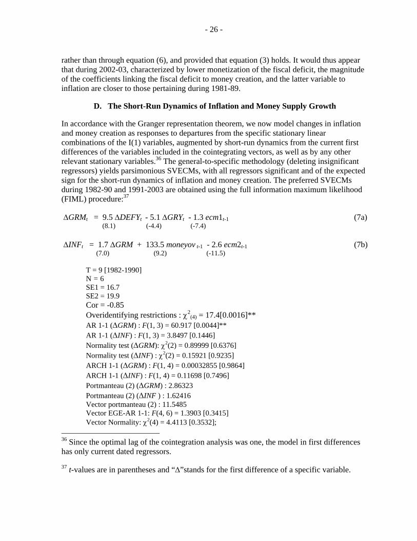
In accordance with the Granger representation theorem, we now model changes in inflation and money creation as responses to departures from the specific stationary linear combinations of the I(1) variables, augmented by short-run dynamics from the current first differences of the variables included in the cointegrating vectors, as well as by any other relevant stationary variables.36 The general-to-specific methodology (deleting insignificant regressors) yields parsimonious SVECMs, with all regressors significant and of the expected sign for the short-run dynamics of inflation and money creation. The preferred SVECMs during 1982-90 and 1991-2003 are obtained using the full information maximum likelihood (FIML) procedure:37

∆GRMt = 9.5 ∆DEFYt - 5.1 ∆GRYt - 1.3 ecm1t-1 (7a) (8.1) (-4.4) (-7.4)

∆INFt = 1.7 ∆GRM + 133.5 moneyov t-1 - 2.6 ecm2t-1 (7b) (7.0) (9.2) (-11.5) T = 9 [1982-1990] N = 6 SE1 = 16.7 SE2 = 19.9 Cor = -0.85

Overidentifying restrictions : χ2(4) = 17.4[0.0016]**

AR 1-1 (∆GRM) : F(1, 3) = 60.917 [0.0044]** AR 1-1 (∆INF) : F(1, 3) = 3.8497 [0.1446] Normality test (∆GRM): χ2(2) = 0.89999 [0.6376]

Normality test (∆INF) : χ2(2) = 0.15921 [0.9235] ARCH 1-1 (∆GRM) : F(1, 4) = 0.00032855 [0.9864]

ARCH 1-1 (∆INF) : F(1, 4) = 0.11698 [0.7496] Portmanteau (2) (∆GRM) : 2.86323 Portmanteau (2) (∆INF ) : 1.62416 Vector portmanteau (2) : 11.5485 Vector EGE-AR 1-1: F(4, 6) = 1.3903 [0.3415] Vector Normality: χ2(4) = 4.4113 [0.3532];

36 Since the optimal lag of the cointegration analysis was one, the model in first differences has only current dated regressors.

37 t-values are in parentheses and “∆”stands for the first difference of a specific variable.

- 27 -

and

∆GRMt = 151.6 ∆DEFYt - 1.1 ecm3t-1 - 1174.9 D93 + 3466.9 D94 (8a) (4.9) (-13.2) (-3.0) (6.8)

∆INFt = 1.1 ∆GRM t + 1572.1 moneyov t-1 - 2.7 ecm4t-1 - 5990.6 D93 + 4365.3 D94 (8b) (6.0) (2.5) (-6.2) (-3.0) (3.8) T = 13 [1991-2003] N = 9 SE1 = 389.1 SE2 = 827.6 Cor = -0.62

Overidentifying restrictions : χ2(5) = 1.17[0.2086]

AR 1-1 (∆GRM) : F(1, 5) = 6.6488 [0.0495]* AR 1-1 (∆INF) : F(1, 5) = 1.7599 [0.2420] Normality test (∆GRM): χ2(2) = 0.23393 [0.8896] Normality test (∆INF) : χ2(2) = 6.0008 [0.0498]* ARCH 1-1 (∆GRM) : F(1, 7) = 1.4104 [0.2737]

ARCH 1-1 (∆INF) : F(1, 7) = 5.7192 [0.0481]* Portmanteau (2) (∆GRM) : 2.32425 Portmanteau (2) (∆INF ) : 0.286915 Vector portmanteau (2) : 9.32806 Vector EGE-AR 1-1: F(4, 12) = 4.0120 [0.0272]* Vector Normality: χ2(4) = 5.3227 [0.2558];

where T is the number of observations, N is the number of parameters, Cor is the correlation of structural residuals, and SE1 and SE2 are the standard deviation of the residuals of the first and second regressions, respectively.38 The definitions of the remaining statistics are provided below. Constant terms are not shown in both systems of equations since they are embedded in the error-correction terms (ecm1, ecm2, ecm3, and ecm4).

38ecm1 = GRM - 7.0*DEFY + 11.6*GRY + constant; ecm2 = INF – 1.2*GRM + constant; ecm3 = GRM - 221.0*DEFY + constant; and ecm4 = INF – 1.5*GRM + constant. The variable moneyov = exp[(m - p) - 1.5 y + 0.26 ∆p] is a measure of “monetary overhang,” that is, the deviation of real money balances from their long-run equilibrium level. It is the error-correction term of a VAR(1) systems including money (m), real income (y), and the opportunity cost of holding money (∆p); m and y are respectively the natural logarithms of money and income, while ∆p is proxied by the rate of inflation. See Nachega (2005). Note that since this money demand function forms a stable cointegrating relationship the monetary overhang is a stationary variable. See, for instance, Altimari (2001) and Nachega (2001).

- 28 -

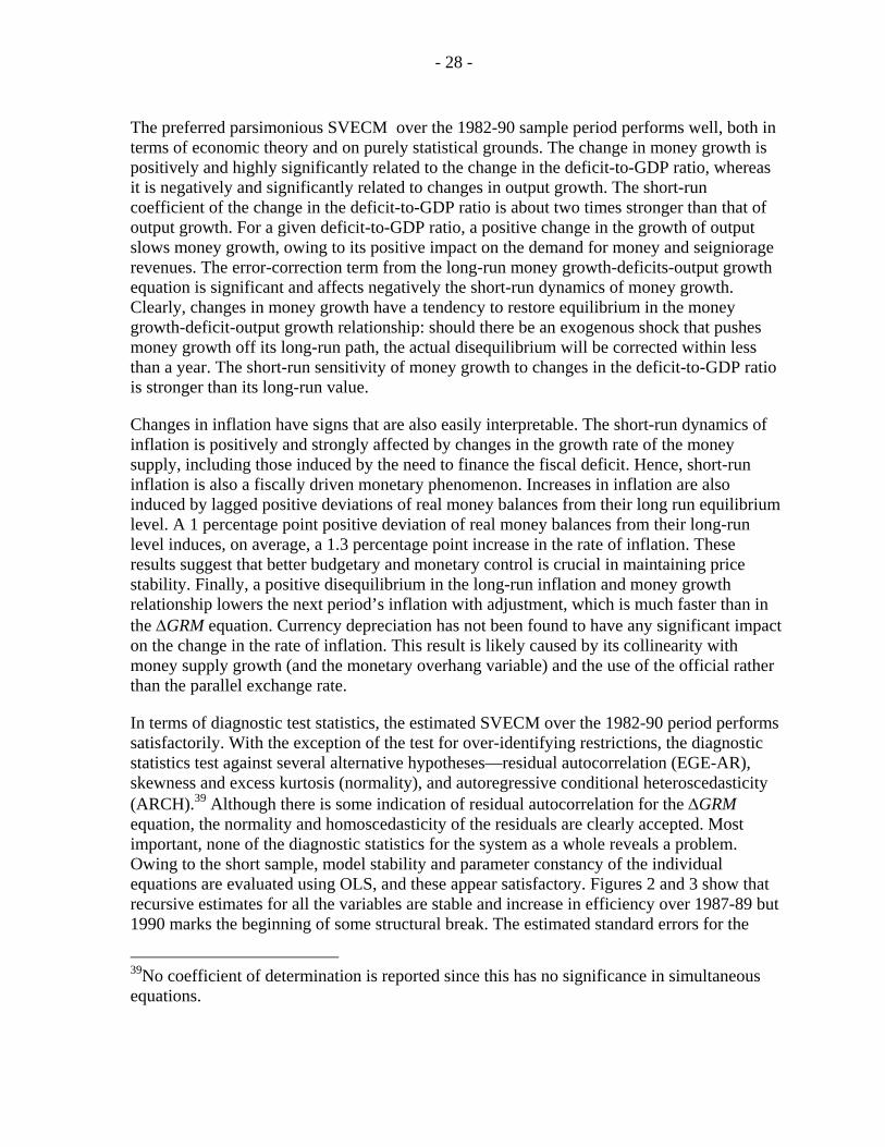
The preferred parsimonious SVECM over the 1982-90 sample period performs well, both in terms of economic theory and on purely statistical grounds. The change in money growth is positively and highly significantly related to the change in the deficit-to-GDP ratio, whereas it is negatively and significantly related to changes in output growth. The short-run coefficient of the change in the deficit-to-GDP ratio is about two times stronger than that of output growth. For a given deficit-to-GDP ratio, a positive change in the growth of output slows money growth, owing to its positive impact on the demand for money and seigniorage revenues. The error-correction term from the long-run money growth-deficits-output growth equation is significant and affects negatively the short-run dynamics of money growth. Clearly, changes in money growth have a tendency to restore equilibrium in the money growth-deficit-output growth relationship: should there be an exogenous shock that pushes money growth off its long-run path, the actual disequilibrium will be corrected within less than a year. The short-run sensitivity of money growth to changes in the deficit-to-GDP ratio is stronger than its long-run value.

Changes in inflation have signs that are also easily interpretable. The short-run dynamics of inflation is positively and strongly affected by changes in the growth rate of the money supply, including those induced by the need to finance the fiscal deficit. Hence, short-run inflation is also a fiscally driven monetary phenomenon. Increases in inflation are also induced by lagged positive deviations of real money balances from their long run equilibrium level. A 1 percentage point positive deviation of real money balances from their long-run level induces, on average, a 1.3 percentage point increase in the rate of inflation. These results suggest that better budgetary and monetary control is crucial in maintaining price stability. Finally, a positive disequilibrium in the long-run inflation and money growth relationship lowers the next period’s inflation with adjustment, which is much faster than in the ∆GRM equation. Currency depreciation has not been found to have any significant impact on the change in the rate of inflation. This result is likely caused by its collinearity with money supply growth (and the monetary overhang variable) and the use of the official rather than the parallel exchange rate.

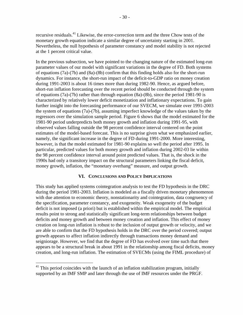
In terms of diagnostic test statistics, the estimated SVECM over the 1982-90 period performs satisfactorily. With the exception of the test for over-identifying restrictions, the diagnostic statistics test against several alternative hypotheses—residual autocorrelation (EGE-AR), skewness and excess kurtosis (normality), and autoregressive conditional heteroscedasticity (ARCH).39 Although there is some indication of residual autocorrelation for the ∆GRM equation, the normality and homoscedasticity of the residuals are clearly accepted. Most important, none of the diagnostic statistics for the system as a whole reveals a problem. Owing to the short sample, model stability and parameter constancy of the individual equations are evaluated using OLS, and these appear satisfactory. Figures 2 and 3 show that recursive estimates for all the variables are stable and increase in efficiency over 1987-89 but 1990 marks the beginning of some structural break. The estimated standard errors for the

39No coefficient of determination is reported since this has no significance in simultaneous equations.

- 29 -

coefficients on moneyov t-1 and ecm2t-1 increase markedly (rather than decrease), and the estimated coefficients for all variables move upward in absolute value indicating faster adjustment or stronger responsiveness (although they remain inside the previously estimated 95 percent confidence intervals). The recursive residuals and the three Chow tests indicate a similar pattern.

The preferred SVECM over 1991-2003 also performs well in terms of economic theory. The change in money growth is positively and highly significantly related to changes in the deficit-to-GDP ratio. The short-run coefficient of the change in the deficit-to-GDP ratio is more than fifteen times higher than during the period 1982-90. For a given deficit-to-GDP ratio, a 1 percentage point positive deviation of real money balances from their long-run level induces about 16 percentage points increase in the next period’s rate of inflation. The error-correction term from the long-run money growth-deficit equation is significant and affects negatively the short-run dynamics of money growth. Should there be an exogenous shock that pushes money growth off its long-run path, the actual disequilibrium will be corrected within less than a year. The short-run sensitivity of money growth to changes in the deficit-to-GDP ratio is weaker than in the long run. This is in contrast to the 1982-90 period.

The inflation equation during 1991-2003 also has signs that are highly significant and easily interpretable. The short-run dynamics of inflation is positively affected by changes in the growth rate of the money supply, including those induced by the need to finance the fiscal deficit and, equally important, by the measure of “monetary overhang.” Hence, the short-run dynamics of inflation during 1991-2003 is also a fiscally driven monetary phenomenon. 40 Increases in inflation are also induced by positive disequilibrium in the money market. These results suggest that fiscal and monetary laxity has played a major role in determining short-run inflation during 1991-2003. Finally, a positive disequilibrium in the long-run inflation/money growth equation lowers the next period’s inflation with adjustment, which is more than two times fast than in the change in the M2 growth equation.

The preferred SVECM in the 1991-2003 sample performs relatively less well on statistical grounds, as suggested by the diagnostic tests. However, with the exception of the vector test for residual autocorrelation, none of the diagnostic statistics for the system as a whole reveals a problem. Model stability and parameter constancy of the individual equations (using OLS) appear satisfactory. While Figure 5 shows that recursive estimates for all the variables of the inflation equation are stable and increase in efficiency over 1995-2003, Figure 4 reveals a significant reduction in the short-run impact of the deficit on the growth rate of the money supply over 2001-03, which translates into some relative increase in the uncertainty of

40 It was found necessary to include two separate dummies labeled D93 and D94 (that took on a value of 1 in 1993 and 1994) to account for the failed monetary reform and introduction of a new currency and a (brief period of) fixed exchange rate regime in late 1993-early 1994. From a statistical point of view, the two dummies were necessary to account for outliers in the equations determining money growth and inflation.

- 30 -

recursive residuals.41 Likewise, the error-correction term and the three Chow tests of the monetary growth equation indicate a similar degree of uncertainty starting in 2001. Nevertheless, the null hypothesis of parameter constancy and model stability is not rejected at the 1 percent critical value.

In the previous subsection, we have pointed to the changing nature of the estimated long-run parameter values of our model with significant variations in the degree of FD. Both systems of equations (7a)-(7b) and (8a)-(8b) confirm that this finding holds also for the short-run dynamics. For instance, the short-run impact of the deficit-to-GDP ratio on money creation during 1991-2003 is about 16 times more than during 1982-90. Hence, as argued before, short-run inflation forecasting over the recent period should be conducted through the system of equations (7a)-(7b) rather than through equation (8a)-(8b), since the period 1981-90 is characterized by relatively lower deficit monetization and inflationary expectations. To gain further insight into the forecasting performance of our SVECM, we simulate over 1991-2003 the system of equations (7a)-(7b), assuming imperfect knowledge of the values taken by the regressors over the simulation sample period. Figure 6 shows that the model estimated for the 1981-90 period underpredicts both money growth and inflation during 1991-95, with observed values falling outside the 98 percent confidence interval centered on the point estimates of the model-based forecast. This is no surprise given what we emphasized earlier, namely, the significant increase in the degree of FD during 1991-2000. More interesting, however, is that the model estimated for 1981-90 explains so well the period after 1995. In particular, predicted values for both money growth and inflation during 2002-03 lie within the 98 percent confidence interval around point predicted values. That is, the shock in the 1990s had only a transitory impact on the structural parameters linking the fiscal deficit, money growth, inflation, the “monetary overhang” measure, and output growth.

VI. CONCLUSIONS AND POLICY IMPLICATIONS

This study has applied systems cointegration analysis to test the FD hypothesis in the DRC during the period 1981-2003. Inflation is modeled as a fiscally driven monetary phenomenon with due attention to economic theory, nonstationarity and cointegration, data congruency of the specification, parameter constancy, and exogeneity. Weak exogeneity of the budget deficit is not imposed (a priori) but is established within the empirical model. The empirical results point to strong and statistically significant long-term relationships between budget deficits and money growth and between money creation and inflation. This effect of money creation on long-run inflation is robust to the inclusion of output growth or velocity, and we are able to confirm that the FD hypothesis holds in the DRC over the period covered; output growth appears to affect inflation indirectly through transactions money demand and seigniorage. However, we find that the degree of FD has evolved over time such that there appears to be a structural break in about 1991 in the relationship among fiscal deficits, money creation, and long-run inflation. The estimation of SVECMs (using the FIML procedure) of

41 This period coincides with the launch of an inflation stabilization program, initially supported by an IMF SMP and later through the use of IMF resources under the PRGF.

- 31 -

inflation and money creation during 1982-90 and 1991-2003 reveals that although the FD hypothesis holds for both periods, it intensified during 1991-2000 before significantly decreasing during the 2001-03 stabilization period. In addition, changes in “monetary overhang” and in income growth have also played significant roles in the short-run dynamics of money creation and inflation. Furthermore, recursive estimates for the period 1991-2003 indicate significant reductions in the magnitude of the coefficient of the deficit on the money supply during 2001-03.

In the 1980s and 1990s, the DRC experienced large and persistent budget deficits, which were monetized by the central bank, resulting in a rapidly increasing money supply, extreme currency depreciation, high inflation, and hyperinflation. These developments were reversed in the early 2000s, as the reorientation of fiscal, monetary, and exchange rate policies, as well as relative political stability and the support of the international financial community (including the IMF) led to a marked fall in inflation and the resumption of economic growth. It is shown that the disinflation process the DRC experienced in the early 2000s was due mainly to the curtailing of fiscal deficits and the decline in the rate of monetary expansion.

From a policy perspective, curtailing FD is key to achieving and maintaining long-term price stability in the DRC. This requires a credible and sustained fiscal adjustment, supported by an appropriate monetary policy. With respect to public finance, a comprehensive tax reform (expanding the tax base, designing an inflation-proof tax system, and improving tax administration and collection), rationalization of public spending, and privatization of loss-making state enterprises are crucial in establishing fiscal policy credibility. Fiscal credibility can also be strengthened through enhanced central bank independence, with a clear mandate to maintain price stability as the overriding objective of monetary policy.

- 32 - APPENDIX

APPENDIX I. DEFINITIONS AND SOURCES OF VARIABLES

The data series are from the IMF World Economic Outlook (WEO) and Information Notice System (INS) databases. INF: inflation, measured as the rate of change of the consumer price index (in percent; end-of-period). Source: WEO. DEFY : overall fiscal deficit (on a commitment basis) in percent of GDP. Source: WEO. VELO: broad money velocity (nominal GDP divided by broad money). Source: WEO. GRM: rate of change of nominal broad money (in percent). Source: WEO. SEIY: seigniorage, measured as the change in broad money divided by GDP (in percent). Source: WEO. GREX : rate of change of the nominal effective exchange rate index (in percent; end-of-period). Source: INS.

- 33 -

1987

1988

1989

1990

51015

Figu

re 2

. Erro

r-Cor

rect

ion

Mod

el (E

CM

) for

Mon

ey G

row

th I:

Rec

ursi

ve E

stim

ates

and

Sta

bilit

y T

ests

Cha

nges

in th

e de

ficit-

to-G

DP

ratio

× +

/-2SE

1987

1988

1989

1990

-10.

0

-7.5

-5.0

-2.50.0

Cha

nges

in o

utpu

t gro

wth

× +

/-2SE

1987

1988

1989

1990

-1.0

-0.50.0

ecm

1_1

× +/

-2SE

1987

1988

1989

1990

-25025

One

-ste

p re

sidu

al

1987

1988

1989

1990

0.5

1.0

1up

CH

OW

s

1%

1987

1988

1989

1990

0.5

1.0

Ndn

CH

OW

s 1

perc

ent c

rit.

1987

1988

1989

1990

0.25

0.50

0.75

1.00

Nup

CH

OW

s 1

perc

ent c

rit.

- 34 -

1986

1987

1988

1989

1990

1.5

2.0

2.5

Figu

re 3

. EC

M fo

r Inf

latio

n I:

Rec

ursi

ve E

stim

ates

and

Sta

bilit

y T

ests

Chan

ges i

n m

oney

gro

wth

× +

/-2SE

1986

1987

1988

1989

1990

-2.5

-2.0

-1.5

ecm

2_1

× +/

-2SE

1986

1987

1988

1989

1990

100

150

Mon

etar

y ov

erha

ng ×

+/-2

SE

1986

1987

1988

1989

1990

-25025

One

-ste

p re

sidua

l

1986

1987

1988

1989

1990

0.5

1.0

1up

CHO

Ws

1 pe

rcen

t crit

.

1986

1987

1988

1989

1990

0.5

1.0

Ndn

CH

OW

s 1

perc

ent c

rit.

1986

1987

1988

1989

1990

0.5

1.0

Nup

CH

OW

s 1

perc

ent c

rit.

- 35 -

1996

1997

1998

1999

2000

2001

2002

2003

100

150

200

Figu

re 4

. EC

M f

or M

oney

Gro

wth

II:

Rec

ursi

ve E

stim

ates

and

Sta

bilit

y T

ests

Cha

nges

in th

e de

fici

t-to

-GD

P r

atio

× +

/-2S

E

1996

1997

1998

1999

2000

2001

2002

2003

-200

0

-150

0

-100

0

-500

D93

× +

/-2S

E

1996

1997

1998

1999

2000

2001

2002

2003

3000

4000

D94

× +

/-2S

E

1996

1997

1998

1999

2000

2001

2002

2003

-1.3

-1.2

-1.1

-1.0

ecm

3_1

× +

/-2S

E

1996

1997

1998

1999

2000

2001

2002

2003

-5000

500

1000

One

-ste

p re

sidu

al

1996

1997

1998

1999

2000

2001

2002

2003

0.5

1.0

1up

CH

OW

s 1

perc

ent c

rit.

1996

1997

1998

1999

2000

2001

2002

2003

0.5

1.0

Ndn

CH

OW

s 1

perc

ent c

rit.

1996

1997

1998

1999

2000

2001

2002

2003

0.5

1.0

Nup

CH

OW

s 1

perc

ent c

rit.

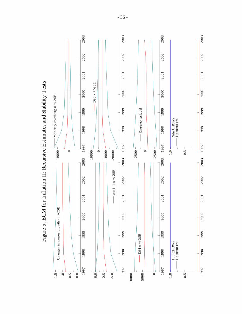
- 36 -

1997

1998

1999

2000

2001

2002

2003

0.0

0.5

1.0

1.5

Figu

re 5

. ECM

for I

nfla

tion

II: R

ecur

sive

Estim

ates

and

Sta

bilit

y T

ests

Cha

nges

in m

oney

gro

wth

× +

/-2SE

1997

1998

1999

2000

2001

2002

2003

0

1000

0M

onet

ary

over

hang

× +

/-2SE

1997

1998

1999

2000

2001

2002

2003

-5.0

-2.50.0

ecm

4_1

× +/

-2SE

1997

1998

1999

2000

2001

2002

2003

-200

00

-100

000

1000

0D

93 ×

+/-2

SE

1997

1998

1999

2000

2001

2002

2003

0

5000

1000

0

D94

× +

/-2SE

1997

1998

1999

2000

2001

2002

2003

-250

00

2500

One

-ste

p re

sidu

al

1997

1998

1999

2000

2001

2002

2003

0.5

1.0

1up

CH

OW

s 1

perc

ent c

rit.

1997

1998

1999

2000

2001

2002

2003

0.5

1.0

Ndn

CH

OW

s 1

perc

ent c

rit.

- 37 -

1988

1989

1990

1991

1992

1993

1994

1995

1996

1997

1998

1999

2000

2001

2002

2003

-750

0

-500

0

-250

00

2500

Figu

re 6

. A

ctua

l and

For

ecas

t C

hang

es in

Mon

ey G

row

th a

nd I

nfla

tion

Fore

cast

cha

nges

in m

oney

gro

wth

A

ctua

l cha

nges

in m

oney

gro

wth

1988

1989

1990

1991

1992

1993

1994

1995

1996

1997

1998

1999

2000

2001

2002

2003

-200

00

-100

000

Fore

cast

cha

nges

in in

flat

ion

Act

ual c

hang

es in

infl

atio

n

- 38 -

References

Aghevli, Bijan B., and Mohsin S. Khan, 1977, “Inflationary Finance and the Dynamics of Inflation: Indonesia, 1951-72,” American Economic Review, Vol. 67 (3), pp. 390-403

Ahking, F.W., and S.M. Miller, 1985, “The Relationship Between Government Deficits, Money Growth, and Inflation,” Journal of Macroeconomics, Vol. 7, pp. 447-67.

Akitoby, B., 2004, “Empirical Evidence of the Sources of Hyperinflation and Falling Currency,” in Post-Conflict Economics in Sub-Saharan Africa: Lessons from the Democratic Republic of the Congo, ed. by J. A. P. Clément (Washington: International Monetary Fund).

Allen, S.D., and M.D. Smith, 1983, “Government Borrowing and Monetary Accommodation,” Journal of Monetary Economics, Vol. 12 (November), pp. 605-16.

Altimari, S. Nicoletti, 2001, “Does Money Lead Inflation in the Euro Area?,” European Central Bank Working Paper No. 63 (May).

Bailey, Martin J., 1956, “The Welfare Cost of Inflationary Finance,” Journal of Political Economy, Vol. 64, pp. 93–110.

Barro, Robert, 1977, “Unanticipated Money Growth and Unemployment in the United States,” American Economic Review, Vol. 67, No 2 (March), pp. 101-15.

_____ , 1978a, “Unanticipated Money, Output, and the Price Level in the United States,” Journal of Political Economy, Vol. 86, pp. 549-80.

_____ , 1978b, “Comment from an Unreconstructed Ricardian,” Journal of Monetary Economics, Vol. 4, pp. 569-81.

_____ , 1979, “On the Determination of the Public Debt,” Journal of Political Economy, Vol. 87, pp. 940-71.

Barth, James, Robin Sickles, and Philip Wiest, 1982, “Assessing the Impact of Varying Economic Conditions on Federal Reserve Behavior,” Journal of Macroeconomics, (Winter), Vol. 4, No. 1, pp. 47-70.

Beaugrand, Philippe, 1997, “Zaire’s Hyperinflation,” IMF Working Paper 97, 50.

Blanchard, Olivier J. and Stanley Fischer, 1989, Lectures in Macroeconomics, The MIT Press, Cambridge, Massachusetts, and London, England.

Buchanan, James, and R. Wagner, 1977, Democracy in Deficit: The Political Legacy of Lord Keynes, New York: Academy Press.

- 39 -

Cagan, Phillip, 1956, “The Monetary Dynamics of Hyperinflation,” in Studies in the Quantity Theory of Money, ed. by Milton Friedman, University of Chicago Press.

Catao, Luis, and Marco E. Terrones, 2005, “Fiscal Deficits and Inflation,” Journal of Monetary Economics, Vol. 52, pp. 529-54.

Clément, Jean A. P., 2004, Post-Conflict Economics in Sub-Saharan Africa: Lessons from the Democratic Republic of the Congo, International Monetary Fund.

Click, Reid W., 1998, “Seigniorage in a Cross-Section of Countries,” Journal of Money, Banking, and Credit, Vol. 10 (May), pp. 154-71.

Cuckierman, Alex, Sebastian Edwards, and Guido Tabellini, 1992, “Seigniorage and Political Instability,” American Economic Review, Vol. 82 (June), pp. 537-55.

Darrat, Ali, 2000, “Are Budget Deficits Inflationary? A Reconsideration of the Evidence,” Applied Economics Letters, Vol. 7, pp. 633-36.

De Haan, J., and D. Zelhorst, 1990, “The Impact of Government Deficits on Money Growth in Developing Countries,” Journal of International Money and Finance, Vol. 7.

Doornik, Jurgen A. and David F. Hendry, 2001, Modelling Dynamic Systems Using PcGive 10: Volume II (London: Timberlake Consultants LTD).

Dornbusch, R., and S. Fischer, 1981, “Budget Deficits and Inflation,” In Development in an Inflationary World, eds. M.J. Flanders and A. Razin, New York: Academic Press.

_____ , F. Sturznegger, and H. Wolf, 1990, “Extreme Inflation: Dynamics and Stabilization,” Brookings Papers in Economic Activity, Vol. 2, pp. 1-64.

Dwyer, G.P., 1982, “Inflation and Governments Deficits,” Economic Inquiry, Vol. 20, pp. 315-29.

Edwards, S., and G. Tabellini, 1991, “Political Instability, Political Weakness, and Inflation,” National Bureau of Economic Research Working Paper, 3721 (May).

Favero, Carlo A. and Franco Spinelli, 1999, “Deficits, Money Growth and Inflation in Italy: 1875-1994,” Economic Notes, Vol. 28, pp. 43-71.

Fischer, Stanley, Ratna Sahay, and Carlos A.Végh, 2002, “Modern Hyper- and High Inflations,” Journal of Economic Literature, Vol. 45 (September), pp. 837-80.

Friedman, Milton, 1971, “Government Revenue from Inflation,” Journal of Political Economy, Vol 79, pp. 846–56.

Ghartey, Edward E., 2001, “Macroeconomic Instability and Inflationary Financing in Ghana,” Economic Modelling, Vol. 18, pp. 415-33.

- 40 -

Giannaros, D.S., and B.R. Kolluri, 1985, “Deficit Spending, Money, and Inflation: Some International Empirical Evidence,” Journal of Macroeconomics, Vol. 7, pp. 401-17.

Gonzalo, Jesus, 1994, “Five Alternative Methods of Estimating Long-Run Equilibrium Relationships,” Journal of Econometrics, Vol. 60 (January-February), pp. 203-33.

Grier, K.B. and H. E. Neiman, 1987, “Deficits, Politics and Money Growth,” Economic Inquiry, Vol. 25, No. 2 (June), pp. 201-14.

Hamburger, M.J., and B. Zwick, 1981, “Deficits, Money and Inflation,” Journal of Monetary Economics, Vol. 7, pp. 141-50.

Harberger, Arnold C., 1978, “The Primer on Inflation,” Journal of Money, Credit, and Banking, Vol. 10, pp. 505-21.

Herrendorf, Berhold, 1997, “Time Consistent Collection of Optimal Seigniorage: A Unifying Framework,” Journal of Economic Surveys, Vol. 11, pp. 1-46.

Johansen, Soren, 1988, “Statistical Analysis of Cointegration Vectors,” Journal of Economic Dynamics and Control, Vol. 12, (June-September), pp. 231-54.

_____ , and Katarina Juselius, 1990, “Maximum Likelihood Estimation and Inference on Cointegration - with Applications to the Demand for Money,” Oxford Bulletin of Economics and Statistics, Vol. 52 (May), pp. 169-210.

Joines, D. H., 1985, “Deficits and Money Growth in the United States 1872-1983,” Journal of Monetary Economics, Vol. 16, No. 3, pp. 329-51.

Juselius, K., 1992, “Domestic and Foreign Effects on Prices in an Open Economy: The Case of Denmark,” Journal of Policy Modeling (August), Vol. 14, No. 4, pp. 401-28.

Keynes, John M., 1923, A Tract on Monetary Reform, Reprinted by the Royal Economic Society, London, 1971.

Kiakwama, G., and J. Chevalier, 2001, “Democratic Republic of Congo,” in S. Devarajan, D. R. Dollar, and T. Holgrem, ed., Aid and Reform in Africa, (Washington: The World Bank).

King, R. G., and C. I. Plosser, 1985, “Money, Deficit and Inflation,” Carnegie-Rochester Conference on Public Policy,” Vol. 22, pp. 147-96.

Laney, L.O. and Thomas Willet, 1983, “Presidential Politics, Budget Deficits and Monetary Policy in the United States,” Public Choice, Vol. 40, No 1, pp. 53-69.

Levy, Mickey, 1981, “Factors Affecting Monetary Policy in an Area of Inflation,” Journal of Monetary Economics, Vol. 8, No. 3, pp. 351-73.

Lucas, Robert E., 1976, “Policy Evaluation: A Critique,” in Carnegie-Rochester Conference Series, The Phillips Curve, North-Holland, Amsterdam, pp 19-46.

MacKinnon, James G., 1991, “Critical Values for Cointegration Tests,” in Long-Run Economic Relationships: Readings in Cointegration, ed. by Robert F. Engle and C.W.J. Granger (Oxford: Oxford University Press).

- 41 -

Masangu, J-C. Mulongo, 2004, Contributions à l’Assainissment du Système Financier Congolais, Kinshasa: New Goff nv.

Matungulu, Mbuyamu I., 2003, “Democratic Republic of the Congo: An Optimist’s Agenda for Economic Revival and Poverty Alleviation,” International Monetary Fund Survey, Vol. 32, No. 16, pp. 258-60.

McMillin, W. Douglas, and Thomas R. Beard, 1982, “Deficits, Money and Inflation: Comment,” Journal of Monetary Economics, Vol. 10, No. 2, pp. 273-77.

Metin, Kivilcim, 1998, “The Relationship Between Inflation and the Budget Deficit in Turkey,” Journal of Business and Economic Statistics, Vol. 16, pp. 412-22.

Montiel, Peter, 1989, “An Empirical Analysis of High-Inflation Episodes in Argentina,

Brazil, and Israel,” International Monetary Fund, Staff Papers, Vol. 36, pp. 527-49.

Nachega, Jean-Claude, 2001, “Financial Liberalization, Money Demand, and Inflation in Uganda,” International Monetary Fund, Working Paper 01/118, (Washington: International Monetary Fund).

_____ , 2005, “Money Demand, Inflation, and PPP in the Democratic Republic of the Congo,” International Monetary Fund, (forthcoming) Working Paper, (Washington: International Monetary Fund).

Niskanen, W.A., 1978, “Deficits, Government Spending and Inflation: What is the Evidence?” Journal of Monetary Economics, Vol. 4, pp. 591-602.

Olivera, J. H. G., 1967, “Money, Prices, and Fiscal Lags: A Note on the Dynamics of Inflation,” Banca Nazionale del Lavoro, Quarterly Economic Review, Vol. 20, pp. 258–67.

Phelps, Edmund S., 1973, “Inflation in the Theory of Public Finance,” Swedish Journal of Economics, Vol. 75 (January), pp. 67-82.

Sargent, Thomas J., and Neil Wallace, 1981, “Some Unpleasant Monetarist Arithmetic,” Federal Reserve Bank Minneapolis Quarterly Review, Fall, pp. 1-17.

Sowa, Nii K., 1994, “Fiscal Deficits, Output Growth and Inflation Targets in Ghana,” World Development, Vol. 22, No. 8, pp. 1105-17.

Tanzi, Vito, 1977, “Inflation, Lags in Collection and the Real Value of Tax Revenue,” IMF Staff Papers, Vol. 24, No.1.

Taylor, Lance, 1983, Structuralist Macroeconomics, Basic Books, New York.

Tekin-Koru, Ayça and Erdal Ozmen, 2003, “Budget Deficits, Money Growth and Inflation: The Turkish Evidence,” Applied Economics, Vol. 350, pp. 591-96.

- 42 -

Woodford, M., 1995, “Price Level Determinacy without Control of a Monetary Aggregate,” Carnegie-Rochester Conference on Public Policy, Vol. 43 (December), pp. 1-46.

Walsh, Carl E., 1998, Monetary Theory and Policy, The MIT Press, Cambridge, MA.