Contents lists available at SciVerse ScienceDirect

Journal of Monetary Economics

Journal of Monetary Economics 59 (2012) 670–685

0304-39

http://d

n Corr

E-m

URL1 A

stickine2 Ca

entry im

driven e3 A

US infla

journal homepage: www.elsevier.com/locate/jme

Firm entry, markups and the monetary transmission mechanism

Vivien Lewis a,n, Celine Poilly b

a Center for Economic Studies, Catholic University Leuven, Naamsestraat 69, 3000 Leuven, Belgiumb Department of Economics, University of Lausanne, HEC-DEEP, Extranef, Quartier UNIL Dorigny, 1015 Lausanne, Switzerland

a r t i c l e i n f o

Article history:

Received 26 January 2011

Received in revised form

2 October 2012

Accepted 9 October 2012Available online 22 October 2012

32/$ - see front matter & 2012 Elsevier B.V. A

x.doi.org/10.1016/j.jmoneco.2012.10.003

esponding author. Tel.: þ32 16 37372.

ail addresses: vivien.lewis@kuleuven.be (V. Le

: http://sites.google.com/site/vivienjlewis (V.

large literature has documented the counter

ss as one of several potential reasons for this

mpbell and Hopenhayn (2005) document a

proves the capacity of real business cycle m

ntry by Bilbiie et al. (2012) and in a friction

notable exception is Cecioni (2010), who uses

tion.

a b s t r a c t

Two business cycle models with endogenous firm and product entry are estimated by

matching impulse responses to a monetary policy shock. The ‘competition effect’

implies that entry lowers desired markups and dampens inflation. Under translog

preferences, where the substitutability between goods depends on their number, we

find evidence of such an effect. That model generates more countercyclical markups

than Dixit and Stiglitz (1977) monopolistic competition model, where price stickiness is

the only source of markup fluctuations. In contrast, a model with strategic interactions

between oligopolistic firms cannot generate an empirically relevant competition effect

and is statistically equivalent to the Dixit–Stiglitz model.

& 2012 Elsevier B.V. All rights reserved.

1. Introduction

Understanding the monetary transmission mechanism, which describes how interest rate changes affect the rest of theeconomy, is important for central banks. Countercyclical fluctuations in the markup play a key role in this process, drivinginflation and hence aggregate demand.1 In the standard New Keynesian model, these are ascribed solely to pricestickiness; other sources of markup cyclicality are neglected. In particular, firm and product turnover are an important(additional) determinant of markups, both on average and along the business cycle.2 Theoretical models have shown that,by reinforcing the countercyclicality of markups under sticky prices, entry has the potential to magnify the effects ofmonetary policy shocks on inflation and output (Bilbiie et al., 2007; Bergin and Corsetti, 2008). This paper subjects thesticky-price endogenous-entry model to a rigorous empirical evaluation, which is so far missing in the literature.3

We develop, estimate and compare two dynamic stochastic general equilibrium (DSGE) models with endogenous entryand various real and nominal frictions. Entry affects the monetary transmission mechanism through the ‘competitioneffect’. By intensifying competitive pressures, the arrival of an entrant increases demand elasticities and reduces desiredmarkups, i.e. the difference between prices and marginal costs in the absence of price rigidities. This happens eitherbecause of increased substitutability between goods or because of stronger competition between oligopolistic producers.

ll rights reserved.

wis), celine.poilly@unil.ch (C. Poilly).

Lewis).

cyclicality of markups, starting from Bils (1987). Rotemberg and Woodford (1999) point to price

stylized fact.

negative correlation between markups and entry in many sectors of the US economy. Introducing

odels to match the cyclical properties of markups. This has been shown in a model with sunk-cost-

less entry model, with zero profits each period, by Cook (2001).

single-equation estimation methods to show that a rise in the number of firms significantly lowers

V. Lewis, C. Poilly / Journal of Monetary Economics 59 (2012) 670–685 671

The competition effect thus introduces fluctuations in desired markups which are positively related to inflation. Combinedwith procyclical entry, this effect makes markups (more) countercyclical.

Our DSGE models both incorporate the competition effect, but differ in the way preferences and industry structures arespecified. The first model features translog preferences as in Feenstra (2003), where increased entry raises thesubstitutability between goods. In this model, the competition effect is demand-driven. The second model assumesstrategic interactions between oligopolists, where increased entry lowers the price setting power of firms. In that model,the competition effect is supply-driven. We refer to the first model as ‘translog model’ and to the second as ‘SI model’.Another important model feature is ‘love of variety’. By enlarging the range of available goods, entry raises utility. Moreproduct variety implies that a given dollar buys more consumption utility and the welfare-based price index falls.4 In thetranslog model, love of variety is equal to half the net price markup in steady state. In the SI model, we impose constantelasticity of substitution (CES) preferences where the love of variety parameter is separated from the elasticity ofsubstitution between goods (see Benassy, 1996, and the working paper version of Dixit and Stiglitz, 1977).

We estimate the parameters of the translog and SI models by matching selected impulse responses to a monetarypolicy shock obtained from a structural vector autoregression (VAR) model. Our VAR includes US data on net businessformation, markups and profits in addition to a set of standard macroeconomic variables. Our findings can be summarizedas follows. In the translog model, we uncover a significant impact of entry on the dynamics of markups and inflationthrough the competition effect. In contrast, the competition effect is insignificant in the SI model. As a result, the translogmodel generates more markup countercyclicality than the SI model. Even though profits play a prominent role for entrydynamics, both models fall short of replicating the large drop in profits following a monetary contraction. The inability tomatch profits is a well-known shortcoming of fixed-variety models and remains a challenge in the endogenous-entryframework.

We analyze in more detail the estimation results in the SI model. First, we show that the parameter restrictions in thatmodel imply a small competition effect for reasonable calibrations of the deep parameters. Second, we investigate theidentifiability of the love of variety parameter and find evidence of partial identification problems. Third, we demonstratethat the SI model is observationally equivalent to the Dixit and Stiglitz (1977) monopolistic competition model (‘DSmodel’), where the competition effect is nil and love of variety equals the net steady state markup. Finally, we perform amodel comparison exercise and show that the translog model is at least as accurate as the SI–DS model in describing thedynamic responses to a monetary policy shock.

The main contribution of this paper is to compare the ability of two endogenous-entry models to generatecountercyclical markups through the competition effect. We are the first to provide a structural estimate of thecompetition effect in the transmission of monetary policy shocks.

The paper is structured as follows. In Section 2, we estimate the VAR model. Section 3 lays out two DSGE models inlinearized form, while Section 4 explains the minimum distance estimation procedure and presents our results. Section 5contains a number of robustness exercises. Section 6 concludes.

2. VAR evidence

We estimate a VAR(2)-model on log real GDP, log real consumption, wage inflation, price inflation, log net businessformation, log real profits, log markups, commodity price inflation and the nominal interest rate. All variables are linearlydetrended. The data sources are listed in Table 1.

We use US quarterly data over the period 1954Q4–1995Q2. The sample is not updated due to a lack of more recent dataon net business formation. Our model-consistent markup measure is inversely related to the labor share and corrects foroverhead labor, as explained in Section 3. Including commodity prices should help to mitigate the price puzzle by whichinflation rises at first after a monetary contraction. By our recursive identification strategy, all variables except the interestrate are included in the information set of the monetary authority and react to a monetary policy shock with a one-period lag.

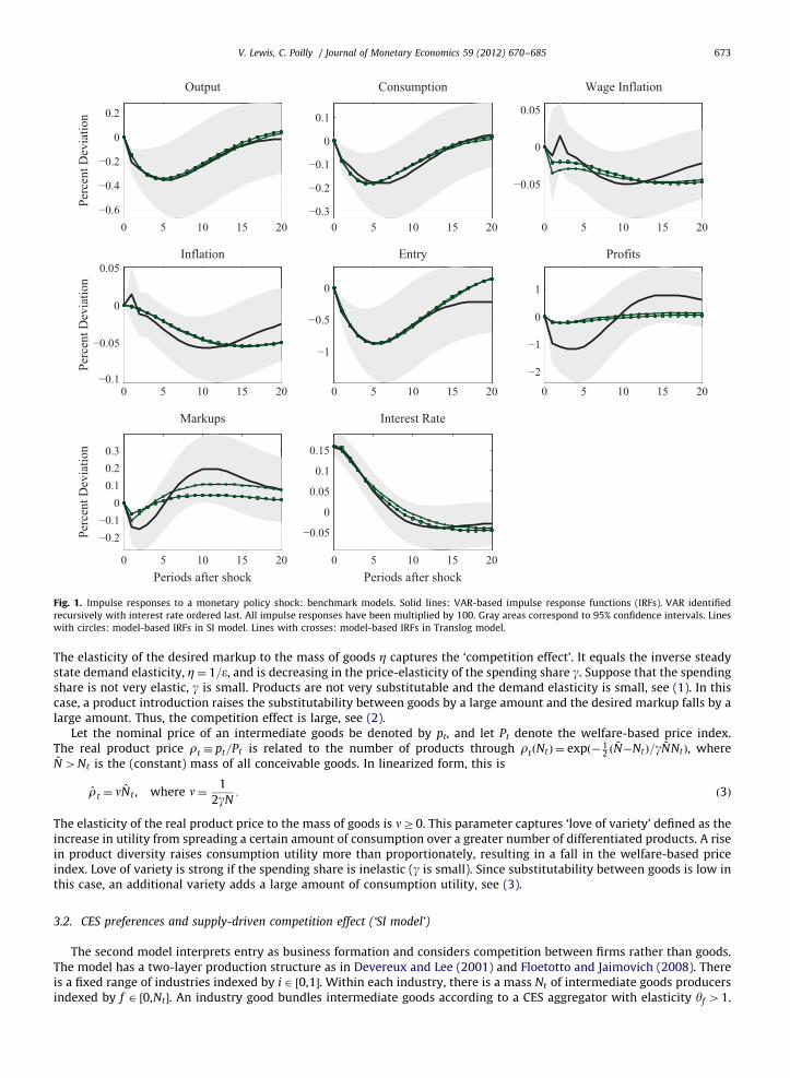
Fig. 1 exhibits the estimated impulse response functions (IRFs) to a contractionary one-standard-deviation monetarypolicy shock. The dynamics of the standard variables are consistent with Christiano et al. (2005). In line with Bergin andCorsetti (2008) and Lewis (2009), the response of net business formation is procyclical and greater than that of output andconsumption. Real profits feature a downward hump-shaped pattern that is significant over four quarters. The response ofmarkups is procyclical on impact and countercyclical at medium horizons.5

3. Two models

We present two DSGE models featuring endogenous entry of firms and goods subject to a fixed labor requirement, aconstant firm exit rate, and sticky prices as in Bilbiie et al. (2012), BGM hereafter. Several empirically motivated frictions

4 Broda and Weinstein (2010) show that product turnover gives rise to a significant cyclical bias in the US price index when consumers have love

of variety.5 This result contrasts with Nekarda and Ramey (2010) who report a procyclical markup response. Their measure of the labor share differs from our

(model-based) measure.

Table 1Data.

(1): Gross Domestic Product BEA

(2): Personal Consumption Expenditures: Services BEA

(3): Personal Consumption Expenditures: Nondurable Goods BEA

(4): Personal Consumption Expenditures BEA

(5): Fixed Private Investment BEA

(6): Government Cons. Expenditures & Gross Investment BEA

(7): Corporate Profits after Taxes, IVA and CCAdj BEA

(8): Compensation of Employees, Paid BEA

(9): Gross Domestic Product: Implicit Price Deflator BEA

(10): Consumer Price Index, all items BLS

(11): Producer Price Index, finished goods BLS

(12): Effective Federal Funds Rate FRB

(13): Compensation Per Hour, nonfarm business sector BLS

(14): All Employees: total nonfarm BLS

(15): Average weekly hours of production workers BLS

(16): Net Business Formation index BEA SCB

(17): CRB Raw Industrials Sub-Index Bridge CRB

Data sources: BEA: Bureau of Economic Analysis. BLS: Bureau of Labor Statistics. FRB: Federal Reserve Board. SCB: Survey

of Current Business. Bridge CRB: Bridge Commodity Research Bureau. Data series: Real GDP is (1)/(9). Real consumption is

(2þ3)/(9). Real physical capital investment is (5)/(9). Real profits are (7)/(9). Wage inflation is the quarter-on-quarter

growth rate of (13). Price inflation is the quarter-on-quarter growth rate of (9). Entry is (16). Commodity price inflation is

the quarter-on-quarter growth rate of (17). The nominal interest rate is (12) at a quarterly rate. The markup is computed

from Eq. (11) in the baseline model and from Eq. (31) in the model with capital. Total hours Lt are average weekly hours

(14), multiplied by the number of employees (15), multiplied by 12 (number of weeks in a quarter). Entry NE,t is (16),

which has been rescaled to be expressed in thousands as Lt, see Appendix B for details. The labor share in total goods

output st

Lis (8)/(4þ6) in the baseline model and (8)/(4þ5þ6) in the model with capital. We set the borrowing cost Rw,t to

(12), which corresponds to a full cost channel (o¼ 1).

V. Lewis, C. Poilly / Journal of Monetary Economics 59 (2012) 670–685672

are added: external habit formation in consumption, sticky wages, price and wage indexation, a cost channel and anendogenous failure rate of entrants.

One may think of entry as product or firm creation; the theoretical literature often uses the two terms interchangeably.Our first model features translog consumption preferences and a demand-driven competition effect through product entry.Our second model assumes CES preferences and a supply-driven competition effect through firm entry.

We consider a symmetric equilibrium with identical households and firms. The timing of events is consistent with therecursive VAR identification scheme. The optimization decisions of households and firms are made before the realizationof the monetary policy shock, except household decisions concerning assets.6 Below, we lay out the model equations inlinearized form.7 A hatted variable denotes its deviation from the deterministic steady state. A variable that has neither ahat nor a time subscript denotes its steady state level.

3.1. Translog preferences and demand-driven competition effect (‘translog model’)

BGM (2012) argue that product turnover is more important than firm turnover for business cycle dynamics. First, firmsthat enter and exit are typically small, such that their impact on industry-wide markups may be limited. Second, productadditions of existing firms matter more for output fluctuations than product innovations of entirely new firms. For thesereasons, BGM (2012) propose a model with translog consumption preferences where demand elasticities depend onproduct diversity. Intuitively, a larger number of differentiated goods makes it easier to substitute among them as theproduct space becomes more crowded.

Under a preference structure as in Feenstra (2003), the price-elasticity of demand is increasing in the mass ofdifferentiated goods Nt,

etðNtÞ ¼ 1þgNt , ð1Þ

where g40 measures the price-elasticity of the spending share on an individual good.8 In contrast with the standard NewKeynesian model, the desired markup here is time-varying, md

t ¼ etðNtÞ=ðetðNtÞ�1Þ. In linearized form, the desired markup is

mdt ¼�ZN t , where Z¼ 1

1þgN: ð2Þ

6 All variables in t (except the interest rate) are chosen on the basis of information in t�1, including forward variables Etfxtþ1g, where Etf�g is the

expectation operator conditional on information in t.7 A model appendix with the full derivation (Appendix A) and a results appendix with robustness checks (Appendix B) are available online.8 All elasticities have been multiplied by �1.

0 5 10 15 20

OutputPe

rcen

t Dev

iatio

n

0 5 10 15 20−0.3

−0.2

−0.1

0

0.1

Consumption

0 5 10 15 20

−0.05

0

0.05

Wage Inflation

0 5 10 15 20

Inflation

Perc

ent D

evia

tion

0 5 10 15 20

−1

−0.5

0

Entry

0 5 10 15 20

−2

−1

0

1

Profits

0 5 10 15 20

−0.6

−0.4

−0.2

0

0.2

−0.1

−0.05

0

0.05

−0.2−0.1

00.10.20.3

Markups

Periods after shock

Perc

ent D

evia

tion

0 5 10 15 20

−0.05

0

0.05

0.1

0.15

Interest Rate

Periods after shock

Fig. 1. Impulse responses to a monetary policy shock: benchmark models. Solid lines: VAR-based impulse response functions (IRFs). VAR identified

recursively with interest rate ordered last. All impulse responses have been multiplied by 100. Gray areas correspond to 95% confidence intervals. Lines

with circles: model-based IRFs in SI model. Lines with crosses: model-based IRFs in Translog model.

V. Lewis, C. Poilly / Journal of Monetary Economics 59 (2012) 670–685 673

The elasticity of the desired markup to the mass of goods Z captures the ‘competition effect’. It equals the inverse steadystate demand elasticity, Z¼ 1=e, and is decreasing in the price-elasticity of the spending share g. Suppose that the spendingshare is not very elastic, g is small. Products are not very substitutable and the demand elasticity is small, see (1). In thiscase, a product introduction raises the substitutability between goods by a large amount and the desired markup falls by alarge amount. Thus, the competition effect is large, see (2).

Let the nominal price of an intermediate goods be denoted by pt, and let Pt denote the welfare-based price index.The real product price rt � pt=Pt is related to the number of products through rtðNtÞ ¼ expð� 1

2 ð~N�NtÞ=g ~NNtÞ, where

~N 4Nt is the (constant) mass of all conceivable goods. In linearized form, this is

rt ¼ nN t , where n¼ 1

2gN: ð3Þ

The elasticity of the real product price to the mass of goods is nZ0. This parameter captures ‘love of variety’ defined as theincrease in utility from spreading a certain amount of consumption over a greater number of differentiated products. A risein product diversity raises consumption utility more than proportionately, resulting in a fall in the welfare-based priceindex. Love of variety is strong if the spending share is inelastic (g is small). Since substitutability between goods is low inthis case, an additional variety adds a large amount of consumption utility, see (3).

3.2. CES preferences and supply-driven competition effect (‘SI model’)

The second model interprets entry as business formation and considers competition between firms rather than goods.The model has a two-layer production structure as in Devereux and Lee (2001) and Floetotto and Jaimovich (2008). Thereis a fixed range of industries indexed by i 2 ½0,1�. Within each industry, there is a mass Nt of intermediate goods producersindexed by f 2 ½0,Nt�. An industry good bundles intermediate goods according to a CES aggregator with elasticity yf 41.

V. Lewis, C. Poilly / Journal of Monetary Economics 59 (2012) 670–685674

The final good is a CES composite of the industry goods with elasticity yi41. The market structure is one of Bertrandcompetition with strategic interactions. Each firm takes into account the effect of its pricing decision on the industry price,taking as given the prices of other firms in the industry and the price levels of other industries. The price-elasticity ofdemand is

etðNtÞ ¼ yf�ðyf�yiÞ1

Nt: ð4Þ

Broda and Weinstein (2006) present empirical evidence that goods are more substitutable within an industry than acrossindustries, yf 4yi. In this case, the firms’ price setting power is eroded by the arrival of new entrants and the demandelasticity increases. The desired markup is decreasing in the mass of firms,

mdt ¼�ZN t , where Z¼

ðyf�yiÞ1N

½yf�ðyf�yiÞ1N�1�½yf�ðyf�yiÞ

1N�: ð5Þ

The competition effect depends positively on the within-industry substitution elasticity yf (relative to the substitutionelasticity across industries, yi). Suppose that goods are not very substitutable, yf is small. Each producer has a large shareof the industry and a lot of monopoly power within an industry, i.e. the demand elasticity is small, see (4). In this case,market shares and hence desired markups do not change much in response to firm entry. Thus, the competition effect issmall, see (5). If goods are as substitutable within as across industries (yf ¼ yi), firm entry has no effect on desired markupsand the competition effect is zero (Z¼ 0), as in the monopolistic competition model of Dixit and Stiglitz (1977).

As in Benassy (1996), we separate love of variety from the elasticity of substitution between goods.9 The real productprice is

rt ¼ nN t , where :

ðaÞ n unrestricted

ðbÞ n¼ 1

yf�1

8><>: : ð6Þ

In our benchmark model, the love of variety parameter n is unrestricted. We also consider the Dixit–Stiglitz preferencestructure, where love of variety is linked to the elasticity of substitution among differentiated goods, n¼ 1=ðyf�1Þ.

3.3. Common model features

Differentiated intermediate goods and new firms NE,t are produced using a linear technology, with labor as the onlyinput. The aggregate production functions in the two sectors are, respectively,

ytþN t ¼ LC,t and NE,t ¼ LE,t : ð7Þ

The variable yt is output per firm, LC,t are hours worked in the sector producing goods and LE,t are hours worked in thesector producing firms. Real marginal costs are cmct ¼ wtþ Rw,t , where wt is the real wage. Because a fraction o 2 ð0,1Þ ofthe wage costs must be paid ahead of production, marginal costs include the interest rate

Rw,t ¼oR

oRþð1�oÞ Rt , ð8Þ

where Rt is the gross rate of return on riskfree nominal bonds. This specification of the cost channel follows Christianoet al. (2010). Total output of goods is obtained by aggregating firm output levels, Y

C

t ¼ rtþ ytþN t . Total goods outputequals private consumption, Y

C

t ¼ C t , since there is neither government spending nor a foreign sector in the model.Aggregate profits depend positively on the actual markup mt and on total goods output,

Dt ¼ ðe�1Þmtþ YC

t : ð9Þ

The pricing decision of intermediate goods producers implies rt ¼ mtþcmct . The variety effect inherent in rt drives a wedgebetween the markup and real marginal costs. As in Rotemberg (1982), we assume that price changes are subject to anadjustment cost proportional to real firm revenues. Price adjustment costs are captured by the parameter kp40.10

We introduce indexation to past inflation as in Ireland (2007). The price adjustment cost is a function of the firm’s pricechange relative to Plp

p,t�1, where Pp,t � pt=pt�1 is product price inflation and lp 2 ð0,1Þ is the degree of indexation. Withsteady state inflation equal to zero, inflation dynamics obey the following New Keynesian Phillips Curve (NKPC)

Pp,t�lpPp,t�1 ¼fpðmdt�mtÞþbð1�dNÞEtfPp,tþ1�lpPp,tg, ð10Þ

where fp ¼ ðe�1Þ=kp and the discount rate bð1�dNÞ is the product of the households’ subjective discount factor b 2 ð0,1Þand the firms’ exogenous survival rate ð1�dNÞ, with dN 2 ð0,1Þ. Through the competition effect, inflation fluctuates

9 The preference structure proposed by Benassy (1996) had previously been explored in the working paper version of Dixit and Stiglitz (1977).10 For simplicity, we assume that entrants, too, face price adjustment costs. BGM (2007) shows that the impulse responses to shocks change

negligibly under the alternative assumption that entrants can change their price costlessly.

V. Lewis, C. Poilly / Journal of Monetary Economics 59 (2012) 670–685 675

inversely with entry. Desired markups depend negatively on the number of competing goods (2) or rather, competingfirms (5). Lower desired markups reduce inflation through the NKPC (10).

The actual markup is inversely related to the labor share stL

and the firms’ borrowing cost, and it corrects for overheadlabor, interpreted here as the share of labor employed in startup activities. Setting startup labor equal to the number ofentrants, we obtain

mt ¼1

ð1�NE,t=LtÞsLt Rw,t

, ð11Þ

where the labor share is the total wage bill over total goods output, sLt ¼ ðwtLt=YC

t Þ.Households maximize expected lifetime utility. Period utility is increasing and concave in consumption with sC Z1

denoting risk aversion. Consumption displays external habit persistence b 2 ð0,1Þ, such that marginal consumption utilityis UC,t ¼�sC=ð1�bÞðC t�bC t�1Þ. Utility is decreasing and convex in hours worked Lt, such that marginal labor disutility isUL,t ¼ sLLt , where sLZ0 is the inverse elasticity of labor supply to the real wage. The household budget constraint is

wtLtþRAt ¼ CtþWACtþAt : ð12Þ

Expenditure includes consumption Ct, wage adjustment costs WACt, and asset purchases

At ¼Bt

PtþwtNE,tþvtEt : ð13Þ

Income includes labor income wtLt and the return on assets,

RAt ¼Rt�1Bt�1

Ptþð1�dNÞðdtþvtÞðEt�1þSt�1NE,t�1Þ: ð14Þ

Households hold three types of assets. First, they buy riskfree nominal one-period bonds Bt at the price of one dollar perbond, which pay a gross return Rt in the next period. The first order condition for bonds is

UC,t ¼ RtþEtf�PC

p,tþ1þUC,tþ1g, ð15Þ

where PC

p,t � Pt=Pt�1 is welfare-based inflation. Second, households buy equity Et at price vt , which they sell one periodlater. The return on equity includes firm profits dt , paid out as dividends, and the capital gain realized in the next period,discounted appropriately, such that the optimality condition on equity is

vt ¼ EtfUC,tþ1�UC,tþ½1�bð1�dNÞ�dtþ1þbð1�dNÞvtþ1g: ð16Þ

Third, households decide on the number of startups and spend wtNE,t on entry costs, where they take the aggregate realwage wt as given. Startups financed one period ago, NE,t�1, survive to period t with probability St�1 as described below.Of those, a constant fraction dN exit; the remaining ones produce and earn profits. Likewise, incumbents exit with aconstant probability dN , such that the dividend on equity holdings Et�1 is ð1�dNÞdt . The value of equity and entrants istherefore ð1�dNÞvt at the end of period t.

In Beaudry et al. (2011), an exogenous expansion of product varieties leads to an inefficient scramble of startups, someof which fail. Following this idea, we assume that only a fraction St of startups becomes operational one period later. Thissuccess probability is specified as

StðNE,t ,NE,t�1Þ ¼ 1�FN,tNE,t

NE,t�1

� �, ð17Þ

where FNð1Þ ¼ F 0Nð1Þ ¼ 0 and F 00Nð1Þ ¼jN 40. Thus, the startup failure rate FN,tð�Þ is an increasing function of the change inentry. It can be interpreted as a flow adjustment cost to extensive margin investment akin to the physical capitalinvestment adjustment cost in Christiano et al. (2005). Mata and Portugal (1994) document that failures of new firms arepositively related to entry rates. As in Lewis (2009), this specification allows us to capture the gradual response of entry toshocks. The free entry condition equates the entry cost wt and the expected value of setting up a firm,

wt ¼ vtStþvtS1tNE,tþbEtUC,tþ1

UC,tvtþ1S2tþ1NE,tþ1

� �, ð18Þ

where Sit is the first derivative of the success rate with respect to its ith argument. The expected value of setting up a firmhas three components. Firm value vt is multiplied by St, the startup success rate. The success rate is in turn negativelyrelated to the change in the number of entrants. A rise in NE,t decreases St and increases the future success rate Stþ1, ceterisparibus. In linearized form, the change in the number of entrants depends positively on its expected future value and onfirm value less the entry cost,

NE,t�NE,t�1 ¼1

jN

ðvt�wtÞþbEtfNE,tþ1�NE,tg: ð19Þ

If entrants face a success probability of 1, we obtain the static free entry condition in BGM (2012), where firm value equalsthe entry cost, vt ¼ wt . The stock of firms evolves according to the law of motion

N tþ1 ¼ ð1�dNÞN tþdNNE,t : ð20Þ

V. Lewis, C. Poilly / Journal of Monetary Economics 59 (2012) 670–685676

We introduce differentiated labor types that are bundled according to a CES aggregator with elasticity yw41. Quadraticwage adjustment costs (captured by kw40) and indexation (captured by lw 2 ð0,1Þ) are introduced, such that wage settingfrictions are analogous to price setting frictions. Wage inflation Pw,t depends positively on its expected future value andon the difference between the marginal rate of substitution between labor and consumption and the real wage. Withindexation, wage inflation also depends on current and lagged price inflation,

Pw,t�lwPp,t�1 ¼fw½ðUL,t�U C,tÞ�wt �þbEtfPw,tþ1�lwPp,tg, ð21Þ

where fw ¼ ððyw�1Þ=kwÞsL. In equilibrium, total labor supply is the sum of labor used in the production of goods and laborused in the production of new firms, weighted by their respective steady state shares, Lt ¼ ðLC=LÞLC,tþðLE=LÞLE,t . LettingYt denote total output, the aggregate accounting identity reads

YC

YY

C

t þvNE

YðwtþNE,tÞ ¼

dN

YðdtþN tÞþ

wL

Yðwtþ LtÞ: ð22Þ

Total expenditure comprises aggregate consumption and investment in new firms. Total income is the sum of dividendincome and labor income.

The central bank adjusts the interest rate in response to inflation and last period’s interest rate. The feedbackcoefficients are tP and tR, such that

Rt ¼ ð1�tRÞtPPp,tþtRRt�1þBt , ð23Þ

where Bt is a first-order autoregressive monetary policy shock with persistence rB and standard error sB. We assume thatmonetary policy stabilizes product prices rather than the welfare-based price index. The latter is typically not observed.Moreover, BGM (2007) and Bergin and Corsetti (2008) show that this is optimal in the presence of appropriate correctivefiscal policies.

4. Estimation

The welfare-based price index, which takes love of variety into account, is unobserved in the data. Measured priceindexes are based on consumption baskets that are infrequently updated and do not quickly take into account the

introduction of new goods. Consequently, we posit that measured inflation corresponds to the variable Pp,t . In the model,

real variables are deflated by the welfare-based price index Pt. To obtain data-consistent model variables that are deflated

by pt, we divide each real variable by the real product price rt . Defining the generic data-consistent variable zRt ¼ zt�rt ,

the model variables that correspond to the series used in our VAR are YR

t , CR

t , Pw,t , Pp,t , NE,t , DR

t , mt , and Rt .

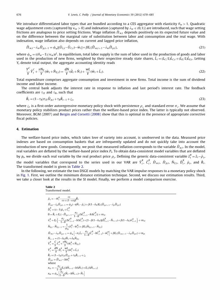
The transformed model is given in Table 2.In the following, we estimate the two DSGE models by matching the VAR impulse responses to a monetary policy shock

in Fig. 1. First, we outline the minimum distance estimation technique. Second, we discuss our estimation results. Third,we take a closer look at the results in the SI model. Finally, we perform a model comparison exercise.

Table 2Transformed model.

m t ¼�wRt �

ooþð1�oÞbRt

Pp,t�lpPp,t�1 ¼fpð�ZN t�m t Þþbð1�dNÞEtfPp,tþ1�lpPp,tg

DR

t ¼ ðe�1Þm tþ CR

t

0¼ RtþEtf�Pp,tþ1�sC

1�bðDC

R

tþ1�bDCR

t Þgþnx1t

vRt ¼ Et �

sC

1�bðDC

R

tþ1�bDCR

t Þþ½1�bð1�dNÞ�ðDR

tþ1�N tþ1Þþbð1�dNÞvRtþ1

n oþnx1t

N E,t�N E,t�1 ¼1

jN

ðvRt �w

Rt ÞþbEtfN E,tþ1�NE,tg

Pw,t�lwPp,t�1 ¼fw �sLLt�sC

1�bðC

R

t �bCR

t�1Þ�wRt

h iþbEtfPw,tþ1�lwPp,tgþnx2t

N tþ1 ¼ ð1�dNÞN tþdNN E,t

YR

t ¼C

YC

R

t þvNE

Yðw

Rt þN E,tÞ

YR

t ¼dN

YD

R

t þwL

Yðw

Rt þ L tÞ

Rt ¼ ð1�tRÞtPPp,tþtRRt�1þBt

Pp,t ¼ Pw,t�DwRt

where

x1t ¼�sC

1�bEtfDN tþ1�bDN tgþEtfDN tþ1g

x2t ¼fw

sC

1�bðN t�bN t�1Þ�N t

h i

Table 3Parameter restrictions.

Translog model SI model

Demand elasticity e¼ 1þgN e¼ yf�ðyf�yiÞ1

NCompetition effect Z¼ 1

1þgN Z¼ðyf�yiÞ

1

N

yf�ðyf�yiÞ1

N�1

� �yf�ðyf�yiÞ

1

N

� �Love of variety n¼ 1

2gN(a) n unrestricted, (b) n¼ 1

yf�1

Slope of NKPCfp ¼

gN

kp fp ¼

yf�ðyf�yiÞ1

N�1

kp

Number of goods/firmsN ¼

z

1þdNz

1�dN

N¼z

1þdNz

1�dN

Note that z¼ ð1=ðe�1ÞÞbð1�dNÞ=ð1�bð1�dNÞÞ½o=bþð1�oÞ�. We impose the additional restriction that N is equal

across models.

V. Lewis, C. Poilly / Journal of Monetary Economics 59 (2012) 670–685 677

4.1. Minimum distance estimation

We fix the parameters b, sL, lp, lw, kp and dN . The subjective discount factor is set to b¼ 0:99, implying a steady statereal interest rate of 4% per annum. Following Christiano et al. (2005), we assume a quadratic labor disutility function,sL ¼ 1, and we impose full indexation of prices and wages, lp ¼ lw ¼ 1. The slope of the New Keynesian Phillips Curvefp contains the price-elasticity of demand e and the price stickiness parameter kp. The demand elasticity is intimatelyrelated to the competition effect, which is our main object of interest. Thus, while it is common to fix the demand elasticityand estimate the degree of price stickiness, we do the opposite here, setting kp ¼ 77 as in BGM (2007).11 Following BGM(2012), the firm exit rate dN is set to 0.025, so as to fit the annual job destruction rate of 10% in the US.

Of the remaining parameters, some are freely estimated, while others are subject to steady state restrictions. Table 3presents the parameter restrictions imposed in the two models.

The parameters are partitioned as ci ¼ ði,KiÞ, where i 2 fT ,SIg indexes the model. The vector

i¼ ðsB,rB,tR,tP,sC ,b,o,fw,jNÞ ð24Þ

is common across models and Ki contains the model-specific parameters. In particular,

KT ¼ ðg,e,Z,n,fp,NÞ and KSI ¼ ðyi,yf ,e,Z,n,fp,NÞ: ð25Þ

In the translog model, the deep parameter is the price-elasticity of the spending share g. In the SI model, the deepparameters are love of variety n and the substitution elasticities yi and yf . Those are the parameters that we estimate. Theother parameters in KT and in KSI must satisfy the restrictions in Table 3. In addition to these model-specific restrictions, weconstrain the steady state number of products N, which is a data-driven object, to be equal across models. We firstestimate the translog model to find NT and then impose the restriction NSI

¼NT in the SI model. In practice, in theestimation of the SI model, yi, yf and o adjust to satisfy the constraint.12 Let the vectors F and FðciÞ denote the VAR-basedand the model-based IRFs, respectively. Parameter estimates c i fulfil

c i ¼ arg minci2Ci

J ðciÞ, ð26Þ

where the distance measure is

J ðciÞ ¼ ½FmðciÞ�F�

0W ½FmðciÞ�F�, ð27Þ

and W is a diagonal matrix with the inverse of the asymptotic variances of each element of F along the diagonal.Following Christiano et al. (2005), the standard errors of the estimated parameters are obtained using the asymptotic deltafunction method applied to the first order condition associated with (26). Since the weighting matrix W is not optimal, theJ-statistic (27) does not have a known distribution. Therefore, we resort to bootstrap techniques (Hall and Horowitz, 1996),adapted to minimum distance estimation of DSGE models by F�eve et al. (2009), to reveal the distribution of the minimumdistance J ðciÞ. We generate 200 bootstrap replications of the VAR model. For each replication, we re-estimate theparameters of the DSGE models and compute the value of the minimum distance. The bootstrapped distribution of thisdistance allows us to test the null hypothesis H0: J ðciÞ ¼ 0. This methodology enables us to check whether the theoreticalmodel passes the overidentification test implied by the choice of moments.

11 Our results are robust to changes in the degree of price stickiness (see Appendix B).12 In Appendix B, we show that our results are unchanged if we impose the cross-model restriction using a joint estimation approach.

Table 4Baseline estimation results.

Translog model SI model, SI model,

(a) n unrestr. (b) n¼ 1=ðyf�1Þ

sB Standard error of shock 0:162ð0:012Þ

0:160ð0:012Þ

0:161ð0:012Þ

rB Autocorrelation of shock 0:877ð0:047Þ

0:829ð0:049Þ

0:833ð0:049Þ

tR Interest rate smoothing 0:046ð0:126Þ

0:180ð0:128Þ

0:170ð0:128Þ

tP Inflation coefficient 1:047ð0:258Þ

1:016ð0:148Þ

1:026ð0:161Þ

sC Risk aversion 3:371ð0:682Þ

2:114ð6:857Þ

1:953ð1:019Þ

b Habit persistence 0:780ð0:057Þ

0:839ð0:542Þ

0:851ð0:080Þ

o Cost channel 0:861ð0:213Þ

0:521ð0:184Þ

0:524ð0:186Þ

fp Slope of price inflation curve 0:019ð0:003Þ

a 0:019ð0:006Þ

a 0:019ð0:006Þ

a

fw Slope of wage inflation curve 0:005ð0:001Þ

0:003ð0:001Þ

0:003ð0:001Þ

jN Adjustment cost (extensive margin) 9:435ð1:852Þ

8:213ð1:721Þ

8:311ð1:656Þ

g Price-elasticity of spending share 0:119ð0:063Þ

– –

yf Substitution elasticity within industries – 2:624ð1:497Þ

2:623ð1:429Þ

yi Substitution elasticity across industries – 1:000ð7:460Þ

1:003ð7:030Þ

e Price-elasticity of demand 2:500ð0:237Þ

a 2:495ð0:457Þ

a 2:495ð0:446Þ

a

Z Competition effect 0:400ð0:038Þ

a 0:034ð0:087Þ

a 0:034ð0:082Þ

a

n Love of variety 0:333ð0:053Þ

a 0:495ð4:195Þ

0:616ð0:271Þ

a

N Number of goods/firms 12:629a 12:629a 12:629a

J -statisticfp-valueg

73:34f0:208g

87:99f0:118g

88:04f0:107g

Baseline estimation results.a Parameter is deduced from steady state restrictions as shown in Table 3. Numbers in round brackets are standard errors. Numbers

in curly brackets are p-values of null hypothesis H0: J ¼ 0.

V. Lewis, C. Poilly / Journal of Monetary Economics 59 (2012) 670–685678

4.2. Results

Fig. 1 displays the IRFs predicted by the translog and SI models, together with the data responses. The performance ofboth models is satisfactory; the p-value in Table 4 indicates that the null hypothesis H0: J ðciÞ ¼ 0 cannot be rejected ineither model.

While the model fit is similar in the two cases, the translog model appears to match better the countercyclical markupdynamics at medium horizons. As in the no-entry model of Christiano et al. (2005), both models fail to reproduce themagnitude of the profit response. This confirms the profit volatility puzzle noted by Colciago and Etro (2010).

The two sets of parameter estimates are reported in Table 4. The hump-shaped response of entry can be replicated onlywith a large adjustment cost parameter: jN is greater than 8 in both models.

The deep parameter of the translog model, the price-elasticity of the spending share, is estimated at g¼ 0:12. In the SImodel, the inter-industry substitution elasticity yi is close to its lower bound of 1, while the intra-industry substitutionelasticity is also fairly low, yf ¼ 2:6. These results determine the size of the demand elasticity, the competition effect andlove of variety, to which we turn next.

The demand elasticity e is close to 2.5 in both models, resulting in a NKPC slope of fp ¼ 0:019. This result is explainedby the small empirical response of the markup. Increasing e raises the marginal cost pass-through fp, which implies fromthe NKPC (10) that markups must move more strongly for a given inflation response.13 We offer two comments on this lowdemand elasticity. First, a high steady state markup is not unreasonable in a model with entry costs. This is because firmsprice at average cost (including entry costs), such that profits in excess of the entry costs are zero in the free-entryequilibrium. Second, in Smets and Wouters’ (2007) model with fixed costs, the estimated steady state markup is 60%,consistent with a demand elasticity of 2.67. This value is close to our estimate.

We note that the models cannot simultaneously match both the markup and profit dynamics. More precisely, the smallinitial drop in markups is incompatible with the large decline in profits. By (9), profits depend positively on the markupresponse and on the demand elasticity, both of which are small. Therefore, while a low e helps to fit markups, it alsoflattens the profit response.

In the translog model, the competition effect is significantly different from zero, Z¼ 0:40. This value implies that if thenumber of goods rises by 1%, desired markups decrease by 0:40%. Fig. 1 shows that the translog model goes some way in

13 If we remove markups from the VAR, the demand elasticity estimate increases to e¼ 5:33 in both models. For more details, see Appendix B.

V. Lewis, C. Poilly / Journal of Monetary Economics 59 (2012) 670–685 679

reproducing the countercyclical markup response at medium horizons. In contrast, the competition effect is insignificantin the SI model, such that firm entry does not generate countercyclical markups. The reason for this result is that theestimated elasticities across and within industries, yi and yf , are both small. The SI model, however, needs a largedifference between these two elasticities in order to produce a competition effect. In Section 4.3, we show that any

empirically plausible calibration of yi and yf implies a small value of Z, given the parameter restrictions of the SI model.Love of variety n is 0.33 in the translog model and 0.49 in the SI model. The estimate in the latter model has a very large

standard error, which may indicate that this parameter is poorly identified.14 In Section 4.3, we perform two exercises todetect potential identification problems. A rise in the number of goods and firms has a positive effect on consumer surplus,by increasing product diversity, and a negative effect on producer surplus, by decreasing profits. These two opposingeffects on welfare cancel out in Dixit and Stiglitz (1977) monopolistic competition model, where love of variety n equalsthe net steady state markup m�1. If n is greater (smaller) than m�1, there is insufficient (excess) entry in equilibrium. Thisdistortion can be removed with an appropriate fiscal or monetary policy.15 In the translog model, love of variety equalshalf the net steady state markup. Therefore, there is excess entry, calling for entry taxes or long run inflation.

Regarding the standard parameters, our estimates are largely consistent with the literature, notably Christiano et al.(2005) and Smets and Wouters (2007). Several results are worth highlighting, though.

The estimates of the cost channel o are 0.86 and 0.52 in the translog and SI model, respectively. In Fig. 1, we observe aprocyclical markup response in the short run. This requires an increase in marginal costs in response to a monetarycontraction, which is delivered through the cost channel as marginal costs rise along with borrowing costs. In the translogmodel, the cost channel must be higher to counteract the competition effect.

The slope of the wage inflation curve is small but significantly different from zero. In an estimated model without entry,the wage inflation curve becomes steeper and hence the implied Calvo wage stickiness parameter is lower.16 As pointedout in Lewis (2009), wage stickiness is key for an endogenous-entry model to generate a negative, and hence empiricallyplausible, response of entry to monetary contractions.

Our estimate of risk aversion is sC ¼ 3:37 in the translog model and sC ¼ 2:11 in the SI model. The markup is morecountercyclical in the translog model due to the competition effect. Real wages, which are inversely related to markups,therefore decrease more in the translog model. Since the real wage represents the price of leisure relative to consumption,this implies a larger drop in consumption for a given elasticity of intertemporal substitution. Put differently, for a givenconsumption response, intertemporal smoothing and therefore sC needs to be higher. Strikingly, the estimates of theutility parameters sC and b, risk aversion and habit formation, have much larger standard errors in the SI model than in thetranslog model. This uncertainty may reflect a partial identification problem in the SI model, to which we turn below.

4.3. A closer look at the SI model

In the SI model, the love of variety estimate is very imprecise, while the competition effect is nil. In this section, weanalyze the reasons for these findings and discuss their implications. We first compute the implied competition effect for arange of plausible substitution elasticities within and across industries. Second, we carry out two diagnostic tests foridentification proposed by Canova and Sala (2009). Third, we test the hypothesis that the SI model is observationallyequivalent to Dixit and Stiglitz (1977) model.

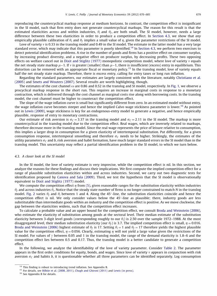
We compute the competition effect Z from (5), given reasonable ranges for the substitution elasticity within industriesyf and across industries yi. Notice that the steady state number of firms is no longer constrained to match N in the translogmodel. Fig. 2 varies yf and yi between 1 and 4. Along the 451-line, the substitution elasticities coincide and hence thecompetition effect is nil. We only consider values below the 451-line as plausible; there, industry goods are lesssubstitutable than intermediate goods within an industry and the competition effect is positive. As we move clockwise, thegap between the elasticities widens, such that the competition effect increases.

To calculate a probable value and an upper bound for the competition effect, we consult Broda and Weinstein (2006),who estimate the elasticity of substitution among goods at the sectoral level. Their median estimate of the substitutionelasticity between 3-digit level goods (corresponding roughly to our yi) is 2.50 over the sample 1972–1988. At the mostdisaggregated level, their median substitution elasticity (our yf ) is 3.7. The implied competition effect is small, Z¼ 0:016.Broda and Weinstein (2006) highest estimate of yf is 17. Setting yi ¼ 1 and yf ¼ 17 therefore yields the highest plausiblevalue for the competition effect, Z¼ 0:056. Clearly, estimating Z will not yield a large value given the restrictions of theSI model. For values of g between 0.05 and 1 in the translog model, the range of the demand elasticity is 1.8–6 and thecompetition effect lies between 0.5 and 0.17. Thus, the translog model is a better candidate to generate a competitioneffect.

In the following, we analyze the identifiability of the love of variety parameter. Consider Table 2. The parameterappears in the first order conditions for equity, bonds, and wages. Since love of variety n appears in conjunction with riskaversion sC and habits b, it is questionable whether all three parameters can be identified separately. Log consumption

14 This finding is robust to introducing trend inflation. See Appendix B.15 For details, see Bilbiie et al. (2008, 2011), Chugh and Ghironi (2011) and Lewis (in press).16 See Appendix B for details.

−0.18685

−0.056055

−0.029896

−0.0074739

00.0074739

0.018685

0.02615

9

0.03237

0.036371 1.5 2 2.5 3 3.5 4

1

1.5

2

2.5

3

3.5

4

Fig. 2. Competition effect in SI model. Figure shows competition effect Z in SI model for different values of inter-industry and intra-industry substitution

elasticities, yi and yf . Discount factor and firm exit rate are set to calibrated values, dN ¼ 0:025 and b¼ 0:99. Cost channel is set to zero, o¼ 0. Assuming a

higher value for o 2 ð0,1Þ has only minor effect on Z since for any o, borrowing cost Rw is close to 1.

V. Lewis, C. Poilly / Journal of Monetary Economics 59 (2012) 670–685680

utility and no habits imply the love of variety parameter drops out from the model.17 In the terminology of Canova andSala (2009), this is a case of under-identification. In a first exercise, we investigate which values of n, sC and b deliver smallchanges in the population objective function computed as

J p ¼ ½FmðcÞ�Fb

ðcÞ�0I½FmðcÞ�Fb

ðcÞ�, ð28Þ

where I is the identity matrix and FmðcÞ are the model-based IRFs under the estimated parameter values displayed in

Table 4, which we will refer to as ‘true’ values. The object FbðcÞ are the model-based IRFs, where we draw 10,000 values of

the three parameters n, sC and b from uniform distributions and the remaining parameters are set to their true values. Theparameters measuring habit formation and love of variety are drawn from a standard uniform distribution; the unitinterval is considered by Bilbiie et al. (2011) as a reasonable range for n. For the risk aversion parameter we consider theinterval ð0,10Þ as our admissible range. We construct the distribution of the distance function (28) and select those drawsthat fall into the lowest 0.1% of that distribution. In Table 5, we report the minimum, the maximum and the median valuesof n, sC and b of the selected draws, together with the true values.

The range between the minimum and the maximum is what Canova and Sala (2009) call the ‘weak identification region’and describes those parameterizations that produce small deviations from the true model. For all three parameters, theweak identification region is large, covering almost the entire admissible range. This suggests that many parametercombinations are compatible with a small objective function. In particular, Dixit–Stiglitz calibration n¼ 1=ðyf�1Þ ¼ 0:62 iscontained within the weak identification region.

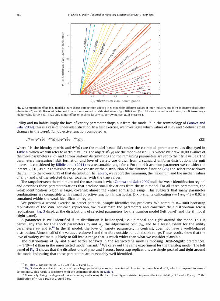
We perform a second exercise to detect potential sample identification problems. We compute n¼1000 bootstrapreplications of the VAR. For each replication, we re-estimate the parameters and construct their distribution acrossreplications. Fig. 3 displays the distributions of selected parameters for the translog model (left panel) and the SI model(right panel).

A parameter is well identified if its distribution is bell-shaped, i.e. unimodal and tight around the mode. This isparticularly true for the shock parameters sB and rB, the adjustment cost jN , and to a lesser extent for the utilityparameters sC and b.18 In the SI model, the love of variety parameter, in contrast, does not have a well-behaveddistribution. Almost half of the values are above 1 and therefore outside our admissible range. These results show that thelove of variety estimate is likely to fall into a range that is much wider than what we consider plausible.

The distributions of sC and b are better behaved in the restricted SI model (imposing Dixit–Stiglitz preferences,n¼ 1=ðyf�1Þ) than in the unrestricted model variant.19 We carry out the same experiment for the translog model. The leftpanel of Fig. 3 shows that the distributions of g, sC and b across bootstrap replications are single-peaked and tight aroundthe mode, indicating that these parameters are reasonably well identified.

17 In Table 2, we see that x1t ¼ x2t ¼ 0 if sC ¼ 1 and b¼0.18 Fig. 3 also shows that in the case of tP , a large probability mass is concentrated close to the lower bound of 1, which is imposed to ensure

determinacy. This result is consistent with the estimates obtained in Table 4.19 Conversely, fixing the degree of risk aversion sC and leaving the love of variety unrestricted improves the identifiability of b and n. For sC ¼ 2, the

distribution of n has a peak at around 0:04.

Table 5Weak identification regions.

Range ‘True’ value Minimum Maximum Median

Love of variety n ½0,1� 0:495 0:000 0:997 0:495

Risk aversion sC ½0,10� 2:114 0:003 9:998 4:972

Habit formation b ½0,1� 0:839 0:000 0:996 0:496

This exercise computes the weak identification regions as in Canova and Sala (2009) for the three utility parameters: love of variety n, risk aversion

sC and habit formation b. We draw values for these parameters simultaneously from uniform distributions, the ranges of which are given in the second

column. The other parameters are held fixed at their estimated (‘true’) values. We construct the distribution of the population distance function (28)

across draws and select those draws for which the population J-statistic falls into the lowest 0.1 percentile. Of the selected draws, we report the

minimum, maximum and median values of n, sC and b.

-0.5 0 0.50

5

10

15

20

0 0.5 10

2

4

6

8

0 5 100

0.1

0.2

0.3

0.4

0 0.50

1

2

3

4

10 20 300

0.02

0.04

0.06

0.08

0.1

0.12

0 0.5 10

5

10

15

1 2 30

5

10

15

0 0.5 10

1

2

3

4

5

0 0.50

5

10

15

20

0 0.5 10

1

2

3

4

5

0 5 100

0.1

0.2

0.3

0.4

0 0.5 10

1

2

3

4

0 10 20 300

0.02

0.04

0.06

0.08

0.1

0.12

0 0.5 10

0.5

1

1.5

2

2.5

3

1 2 30

1

2

3

4

5

0 1 2 30

0.1

0.2

0.3

0.4

0.5

Fig. 3. Parameter distributions across VAR bootstrap replications: Translog model (left panel) and SI model (right panel). We estimate both models using

n¼1000 VAR bootstrap replications. Figure shows distributions of selected parameter estimates across replications. Left panel: Translog model. Right

panel: unrestricted SI model (shaded areas), restricted SI model (solid lines).

V. Lewis, C. Poilly / Journal of Monetary Economics 59 (2012) 670–685 681

In Table 4, we report the estimation results of the restricted SI model where we impose the restriction n¼ 1=ðyf�1Þ.The standard errors of risk aversion sC and habit formation b, are considerably reduced relative to the unrestricted SImodel and are close to the respective standard errors in the translog model. In addition, the overall model fit deterioratesonly slightly; the J-statistic increases only marginally when we impose the restriction.

Taken together, our results suggest that, given our data set and objective function, we cannot separately identify love ofvariety, risk aversion, and the degree of habit formation. Imposing an extra restriction on the love of variety parameter, asin the translog or Dixit–Stiglitz models, helps to identify the other utility parameters. However, even if the populationidentification problem can be overcome by appropriately re-specifying the model, macroeconomic data may fail to containinformation necessary to identify the degree of love of variety. Fundamentally, variety gains are not adequatelyincorporated in cost-of-living measures, as mentioned above. Bils and Klenow (2001) conjecture that ‘quantifying theaggregate importance of new products [...] is probably not feasible’.

Given the lack of a competition effect and the large uncertainty surrounding the love of variety estimate in the SI model,we test formally if the model is observationally equivalent to Dixit and Stiglitz (1977) monopolistic competition model,where yi ¼ yf and n¼ 1=ðyf�1Þ. We perform a distance metric test as in Meier and Muller (2006). The test statistic is given by

J rðc iÞ�J ðc iÞ �a w2ðmÞ, ð29Þ

where J rðc iÞ is the value of the sample J-statistic under the restrictions to be tested and m is the number of restrictions.Since J rðcSIÞ ¼ 90:47, J ðcSIÞ ¼ 87:99 and w2

10%ð2Þ ¼ 4:6, we cannot reject the null hypothesis that the Dixit–Stiglitzrestrictions hold in the SI model at the 10% confidence level.

4.4. Model comparison

This section compares the ability of two models, the translog model and restricted SI model, to replicate the empiricaldynamics of each variable separately. Along the lines of Dupor et al. (2010), Carrillo (2012) proposes the Root MeanSquared Error (RMSE) between the theoretical and empirical impulse responses as a measure of model accuracy. Similarly

0 0.005 0.010

500

1000

1500

2000Output

0 0.005 0.010

200

400

600

800

1000Consumption

0 0.005 0.010

200

400

600

800Wage Inflation

0 0.005 0.010

200

400

600

800Inflation

0 0.005 0.010

100

200

300Entry

0 0.005 0.010

50

100

150Profits

0 0.005 0.010

100

200

300

400Markups

0 0.005 0.010

200

400

600

800Interest Rate

Fig. 4. Root Mean Squared Error (RMSE) distributions across VAR bootstrap replications. We estimate both models using n¼1000 VAR bootstrap replications.

For each variable and bootstrap iteration, Root Mean Squared Error is computed as RMSEix,j ¼

ffiffiffiffiffiffiffiffiffiffiffiffiffiffiffiffiffiffiffiffiffiffiffiffiffiffiffiffiffiffiffiffiffiffiffiffiffiffiffiffiffiffiffiffiffiffiffiffiffiffiffiffiffiffiffiffiffiffiffiffiffiffiffiffiffiffið1=HÞ

PHh ¼ 1ðFx,j,hðc iÞ�Fx,j,hÞ

2q

, j¼ 1, . . .n, where Fx,j,hðc iÞ is

model-based IRF and Fx,j,h is VAR-based IRF of variable x, at horizon h and iteration j. Dashed line: SI model. Dotted line: translog model.

V. Lewis, C. Poilly / Journal of Monetary Economics 59 (2012) 670–685682

to the previous section, the theoretical models are re-estimated on n¼1000 bootstrap replications of the VAR. For eachvariable and bootstrap iteration, we compute the RMSE as

RMSEix,j ¼

ffiffiffiffiffiffiffiffiffiffiffiffiffiffiffiffiffiffiffiffiffiffiffiffiffiffiffiffiffiffiffiffiffiffiffiffiffiffiffiffiffiffiffiffiffiffiffiffiffiffiffiffi1

H

XH

h ¼ 1

ðFx,j,hðc iÞ�Fx,j,hÞ2

vuut , j¼ 1, . . .n, ð30Þ

where Fx,j,hðc iÞ is the model-based IRF and Fx,j,h is the VAR-based IRF of variable x, at horizon h and iteration j. Fig. 4 plotsthe distribution of the RMSE across bootstrap replications.

A distribution close to zero indicates that the model is successful in fitting the variable’s observed dynamics. We findthat the two models perform equally well in matching the impulse responses of most variables, including the markup.Only the output response is predicted more accurately in the translog model; the RMSE distribution is closer to zero.

5. Robustness

Our estimation results have shown that the translog model generates countercyclical markups through the competitioneffect. In order to test the robustness of this finding, Table 6 reports the results of three alternative estimation exercises.20

The first estimates the model using the consumer price index (CPI) and the producer price index (PPI) as alternatives to theGDP deflator. The second estimates the model under non-zero steady state inflation. The third considers capital as a factorof production.21

20 We present analogous exercises for the restricted SI model, i.e. imposing n¼ 1=ðyf�1Þ, in Appendix B.21 Detailed derivations of the models with trend inflation and capital are provided in Appendix A. Notice that the equation determining the steady

state number of firms N changes. In the model with capital, the parameter restrictions on e, Z, n and fp are as in Table 3. In the model with trend inflation,

the restrictions on e, Z, n and fp are different from those in Table 3.

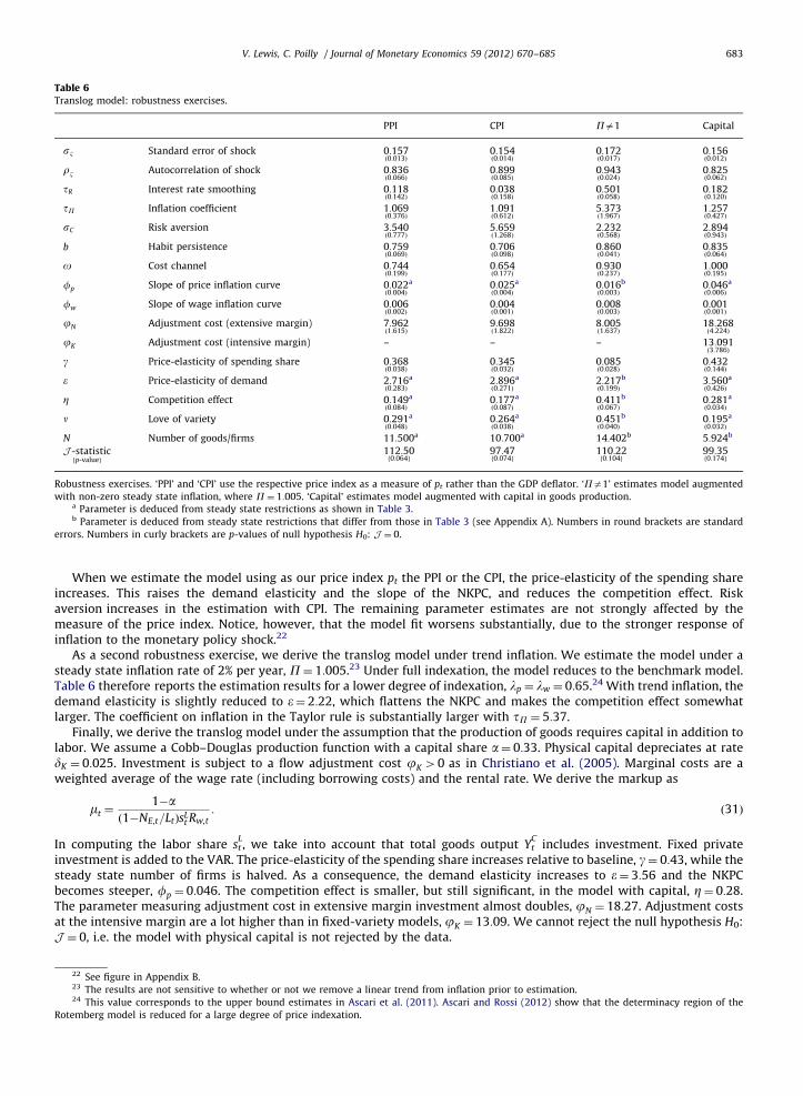
Table 6Translog model: robustness exercises.

PPI CPI Pa1 Capital

sB Standard error of shock 0:157ð0:013Þ

0:154ð0:014Þ

0:172ð0:017Þ

0:156ð0:012Þ

rB Autocorrelation of shock 0:836ð0:066Þ

0:899ð0:085Þ

0:943ð0:024Þ

0:825ð0:062Þ

tR Interest rate smoothing 0:118ð0:142Þ

0:038ð0:158Þ

0:501ð0:058Þ

0:182ð0:120Þ

tP Inflation coefficient 1:069ð0:376Þ

1:091ð0:612Þ

5:373ð1:967Þ

1:257ð0:427Þ

sC Risk aversion 3:540ð0:777Þ

5:659ð1:268Þ

2:232ð0:568Þ

2:894ð0:943Þ

b Habit persistence 0:759ð0:069Þ

0:706ð0:098Þ

0:860ð0:041Þ

0:835ð0:064Þ

o Cost channel 0:744ð0:199Þ

0:654ð0:177Þ

0:930ð0:237Þ

1:000ð0:195Þ

fp Slope of price inflation curve 0:022ð0:004Þ

a 0:025ð0:004Þ

a 0:016ð0:003Þ

b 0:046ð0:006Þ

a

fw Slope of wage inflation curve 0:006ð0:002Þ

0:004ð0:001Þ

0:008ð0:003Þ

0:001ð0:001Þ

jN Adjustment cost (extensive margin) 7:962ð1:615Þ

9:698ð1:822Þ

8:005ð1:637Þ

18:268ð4:224Þ

jK Adjustment cost (intensive margin) – – – 13:091ð3:786Þ

g Price-elasticity of spending share 0:368ð0:038Þ

0:345ð0:032Þ

0:085ð0:028Þ

0:432ð0:144Þ

e Price-elasticity of demand 2:716ð0:283Þ

a 2:896ð0:271Þ

a 2:217ð0:199Þ

b 3:560ð0:426Þ

a

Z Competition effect 0:149ð0:084Þ

a 0:177ð0:087Þ

a 0:411ð0:067Þ

b 0:281ð0:034Þ

a

n Love of variety 0:291ð0:048Þ

a 0:264ð0:038Þ

a 0:451ð0:040Þ

b 0:195ð0:032Þ

a

N Number of goods/firms 11:500a 10:700a 14:402b 5:924b

J -statisticfp-valueg

112:50f0:064g

97:47f0:074g

110:22f0:104g

99:35f0:174g

Robustness exercises. ‘PPI’ and ‘CPI’ use the respective price index as a measure of pt rather than the GDP deflator. ‘Pa1’ estimates model augmented

with non-zero steady state inflation, where P¼ 1:005. ‘Capital’ estimates model augmented with capital in goods production.a Parameter is deduced from steady state restrictions as shown in Table 3.b Parameter is deduced from steady state restrictions that differ from those in Table 3 (see Appendix A). Numbers in round brackets are standard

errors. Numbers in curly brackets are p-values of null hypothesis H0: J ¼ 0.

V. Lewis, C. Poilly / Journal of Monetary Economics 59 (2012) 670–685 683

When we estimate the model using as our price index pt the PPI or the CPI, the price-elasticity of the spending shareincreases. This raises the demand elasticity and the slope of the NKPC, and reduces the competition effect. Riskaversion increases in the estimation with CPI. The remaining parameter estimates are not strongly affected by themeasure of the price index. Notice, however, that the model fit worsens substantially, due to the stronger response ofinflation to the monetary policy shock.22

As a second robustness exercise, we derive the translog model under trend inflation. We estimate the model under asteady state inflation rate of 2% per year, P¼ 1:005.23 Under full indexation, the model reduces to the benchmark model.Table 6 therefore reports the estimation results for a lower degree of indexation, lp ¼ lw ¼ 0:65.24 With trend inflation, thedemand elasticity is slightly reduced to e¼ 2:22, which flattens the NKPC and makes the competition effect somewhatlarger. The coefficient on inflation in the Taylor rule is substantially larger with tP ¼ 5:37.

Finally, we derive the translog model under the assumption that the production of goods requires capital in addition tolabor. We assume a Cobb–Douglas production function with a capital share a¼ 0:33. Physical capital depreciates at ratedK ¼ 0:025. Investment is subject to a flow adjustment cost jK 40 as in Christiano et al. (2005). Marginal costs are aweighted average of the wage rate (including borrowing costs) and the rental rate. We derive the markup as

mt ¼1�a

ð1�NE,t=LtÞsLt Rw,t

: ð31Þ

In computing the labor share stL, we take into account that total goods output Yt

Cincludes investment. Fixed private

investment is added to the VAR. The price-elasticity of the spending share increases relative to baseline, g¼ 0:43, while thesteady state number of firms is halved. As a consequence, the demand elasticity increases to e¼ 3:56 and the NKPCbecomes steeper, fp ¼ 0:046. The competition effect is smaller, but still significant, in the model with capital, Z¼ 0:28.The parameter measuring adjustment cost in extensive margin investment almost doubles, jN ¼ 18:27. Adjustment costsat the intensive margin are a lot higher than in fixed-variety models, jK ¼ 13:09. We cannot reject the null hypothesis H0:J ¼ 0, i.e. the model with physical capital is not rejected by the data.

22 See figure in Appendix B.23 The results are not sensitive to whether or not we remove a linear trend from inflation prior to estimation.24 This value corresponds to the upper bound estimates in Ascari et al. (2011). Ascari and Rossi (2012) show that the determinacy region of the

Rotemberg model is reduced for a large degree of price indexation.

V. Lewis, C. Poilly / Journal of Monetary Economics 59 (2012) 670–685684

6. Conclusion

The present paper considers two business cycle models with endogenous firm and product entry. Through thecompetition effect, entry makes markups more countercyclical. In a model with translog preferences (‘translog model’), thesubstitutability between goods and hence demand elasticities are positively related to product entry. In an alternativemodel with strategic interactions between oligopolists (‘SI model’), firm entry reduces the market power of incumbents.We estimate the models by matching impulse responses to a monetary policy shock in US data, where entry is measuredas net business formation. We find that both models perform equally well in replicating the empirical responses. However,the translog model produces countercyclical markups through a significant competition effect, while the SI model doesnot. This has some bearing on the estimates of certain other parameters, more specifically the degree of risk aversion andthe cost channel. We go on to show that in the SI model, the competition effect is small for any reasonable calibration ofthe substitution elasticities within and across industries. Therefore, that model is observationally equivalent to the Dixit–Stiglitz monopolistic competition model where all markup countercyclicality is due to price stickiness. As an additionalcontribution, we show that an attempt to estimate the love of variety parameter jointly with the degrees of risk aversionand habit persistence is subject to identification problems.

Acknowledgments

Part of this research was funded by the French Agence Nationale de la Recherche (ANR), under Grant ANR-11-JSH1 002 01.Thanks to Florin Bilbiie, Julio Carrillo, Martina Cecioni, Andrea Colciago, Fabrice Collard, Gregory de Walque, Maarten Dossche,Martin Ellison, Stefan Gerlach, Fabio Ghironi, Jean Imbs, Punnoose Jacob, Julien Matheron, Sophocles Mavroeidis, Gert Peersman,Florian Pelgrin, Arnoud Stevens, Roland Winkler, Raf Wouters and an anonymous referee for very useful comments andsuggestions. We are also grateful to participants at various conferences and seminars. All remaining errors are the authors’.

Appendix. Supporting information

Supplementary data associated with this article can be found in the online version at http://dx.doi.org.10.1016/j.jmoneco.2012.10.003.

References

Ascari, G., Rossi, L., 2012. Trend inflation and firms price-setting: Rotemberg Versus Calvo. The Economic Journal 122 (563), 1115–1141.Ascari, G., Castelnuovo, E., Rossi, L., 2011. Calvo vs. Rotemberg in a trend inflation world: an empirical investigation. Journal of Economic Dynamics

and Control 35, 1852–1867.Beaudry, P., Collard, F., Portier, F., 2011. Gold rush fever in business cycles. Journal of Monetary Economics 58 (2), 84–97.Benassy, J.-P., 1996. Taste for variety and optimum production patterns in monopolistic competition. Economics Letters 52 (1), 41–47.Bergin, P., Corsetti, G., 2008. The extensive margin and monetary policy. Journal of Monetary Economics 55 (7), 1222–1237.Bilbiie, F., Fujiwara, I., Ghironi, F., 2011. Optimal Monetary Policy with Endogenous Product Variety. NBER Working Paper 17489.Bilbiie, F., Ghironi, F., Melitz, M., 2012. Endogenous entry, product variety, and business cycles. Journal of Political Economy 120 (2), 304–345.Bilbiie, F., Ghironi, F., Melitz, M., 2008. Monopoly Power and Endogenous Variety in Dynamic General Equilibrium: Distortions and Remedies, NBER

Working Paper 14383.Bilbiie, F., Ghironi, F., Melitz, M., 2007. Monetary policy and business cycles with endogenous entry and product variety. NBER Macroeconomics Annual

22, 299–353.Bils, M., 1987. The cyclical behavior of marginal cost and price. American Economic Review 77 (5), 838–857.Bils, M., Klenow, P.J., 2001. The acceleration in variety growth. American Economic Review Papers and Proceedings 91 (2), 274–280.Broda, C., Weinstein, D.E., 2010. Product creation and destruction: evidence and price implications. American Economic Review 100 (3), 691–723.Broda, C., Weinstein, D.E., 2006. Globalization and the gains from variety. Quarterly Journal of Economics 121 (2), 541–585.Campbell, J.R., Hopenhayn, H.A., 2005. Market size matters. Journal of Industrial Economics 53 (1), 1–25.Canova, F., Sala, L., 2009. Back to square one: identification issues in DSGE models. Journal of Monetary Economics 56 (4), 431–449.Carrillo, J.A., 2012. How well does sticky information explain the dynamics of inflation, output, and real wages? Journal of Economic Dynamics and

Control 36 (6), 830–850.Cecioni, M., 2010. Firm Entry, Competitive Pressures and the U.S. Inflation Dynamics. Temi di discussione (Economic working papers) 773, Bank of Italy.Christiano, L.J., Eichenbaum, M., Evans, C.L., 2005. Nominal rigidities and the dynamic effects of a shock to monetary policy. Journal of Political Economy

113 (1), 1–45.Christiano, L.J., Trabandt, M., Walentin, K., 2010. DSGE models for monetary policy analysis. In: Friedman, B.M., Woodford, M. (Eds.), Handbook

of Monetary Economics, Elsevier, Amsterdam, pp. 285–367.Chugh, S.K., Ghironi, F., 2011. Optimal Fiscal Policy and Endogenous Product Variety. NBER Working Paper 17319.Colciago, A., Etro, F., 2010. Endogenous market structures and the business cycle. Economic Journal 120 (549), 1201–1233.Cook, D., 2001. Time to enter and business cycles. Journal of Economic Dynamics and Control 25, 1241–1261.Devereux, M.B., Lee, K.M., 2001. Dynamic gains from trade with imperfect competition and market power. Review of Development Economics 5 (2),

239–255.Dupor, B., Kitamura, T., Tsuruga, T., 2010. Integrating sticky prices and sticky information. Review of Economics and Statistics 92 (3), 657–669.Dixit, A.K., Stiglitz, J.E., 1977. Monopolistic competition and optimum product diversity. American Economic Review 67 (3), 297–308.Feenstra, R.C., 2003. A homothetic utility function for monopolistic competition models, without constant price elasticity. Economics Letters 78 (1),

79–86.

V. Lewis, C. Poilly / Journal of Monetary Economics 59 (2012) 670–685 685

F�eve, P., Matheron, J., Sahuc, J-G., 2009. Minimum distance estimation and testing of DSGE models from structural VARs. Oxford Bulletin of Economics andStatistics 71 (6), 883–894.

Floetotto, M., Jaimovich, N., 2008. Firm dynamics, markup variations, and the business cycle. Journal of Monetary Economics 55 (7), 1238–1252.Hall, P., Horowitz, J., 1996. Bootstrap critical values for tests based on generalized-method-of-moments estimators. Econometrica 64 (4), 891–916.Ireland, P.N., 2007. Changes in the federal reserve’s inflation target: causes and consequences. Journal of Money, Credit and Banking 39 (8), 1851–1882.Lewis, V. Optimal Monetary Policy and Firm Entry. Macroeconomic Dynamics, http://dx.doi.org/10.1017/S1365100512000272, in press.Lewis, V., 2009. Business cycle evidence on firm entry. Macroeconomic Dynamics 13 (5), 605–624.Mata, J., Portugal, P., 1994. Life duration of new firms. Journal of Industrial Economics 42 (3), 227–245.Meier, A., Muller, G., 2006. Fleshing out the monetary transmission mechanism—output composition and the role of financial frictions. Journal of Money,

Credit, and Banking 38 (8), 2099–2134.Nekarda, C., Ramey, V., 2010. The Cyclical Behavior of the Price-Cost Markup. Manuscript.Rotemberg, J.J., 1982. Monopolistic price adjustment and aggregate output. Review of Economic Studies 49 (4), 517–531.Rotemberg, J.J., Woodford, M., 1999. The cyclical behavior of prices and costs. In: Taylor, J.B., Woodford, M. (Eds.), Handbook of Macroeconomics, Elsevier,

Amsterdam, pp. 1051–1135.Smets, F., Wouters, R., 2007. Shocks and frictions in US business cycles: a Bayesian DSGE approach. American Economic Review 97 (3), 586–606.