Finite element method for structural dynamic and stability...
49
Finite element method for structural dynamic and stability analyses 1 Prof C S Manohar Department of Civil Engineering IISc, Bangalore 560 012 India Module-9 Structural stability analysis Lecture-31 3D beam element; plate element; imperfection sensitive structures; beams on elastic foundation; rings and arches.
Transcript of Finite element method for structural dynamic and stability...

Finite element method for structural dynamic
and stability analyses
1
Prof C S Manohar Department of Civil Engineering
IISc, Bangalore 560 012 India
Module-9
Structural stability analysis
Lecture-31 3D beam element; plate element; imperfection sensitive
structures; beams on elastic foundation; rings and arches.

2
2 22
2
0 0
Euler-Bernoulli beam element
1
2 2
l ld v P dv
U EI dx dxdx dx
P P,EI l
4u
3u
2u
1u
x
y
4
1
i i
i
v x u x
2 2
3
2 2
2 2
2 2
12 6 12 6
6 4 6 2
12 6 12 6
6 2 6 4
36 3 36 3
3 4 3
36 3 36 330
3 3 4
G
l l
l l l lEIK
l ll
l l l l
l l
l l l lPK
l ll
l l l l

3
2 2 2
0 0
0 0 0
0 0 0
1
2
0 01
0 0 with =2
0 0
xx zx
V
e e e
xx xy xz
t
xy yy yz
V
u v w u u v v w wU dV
x x x y z y z y z
u
u
v N u N u G u
w
s
U s dV s
s
0 0 0
0 01
0 02
0 0
0 01
with 0 0 Geometric stiffness matrix2
0 0
xz yz zz
tt t
e e e e
V
t
V
s
U u G s G u dV u K u
s
s
K G s G dV
s

4
Axially deforming rod
l l
,x u ,x u
,z w ,z w
2u
2w
2
121
1 1 2 2
1 1 2 2
1 2;
u x N u N u
w x N w N w
l x xN N
x l
0
1 0 1 01
0 1 0 1
1 0 1 0
0 1 0 1
1 0 1 0
0 1 0 1
with xx
Gl
PK
L
P A

5
0 0 0 0
0 0
0 0
1
2 2
1
2 2
1
2 2
t t
t t t t
t t
t
t
PV t u t Ku t u Ju
Pu T KT u u T JT u
Pu Ku u Ju
K T KT
J T JT
Element stiffness matrix in the transformed coordinate system
Element stability matrix in the transformed coordinate system
K
J
Local to global
coordinate
transformation

6
How to analyse this type of problems?

7
1
Step-1 Assemble the reduced structure elastic stiffness matrix and
equivalent nodal force vector .
Step-2 Find response and determine the ax
K
F
X K F
Recipe for finding critical load for planar frames
ial thrust diagram
for the structure.
Step-3 Using the axial thrust information in the above step, formulate the
reduced structural geometric stiffness matrix
Step-4 Solve the eigenvalue problem
GK
K K
min
min
and estimate the lowest
eigenvalue, .
factor by which the prevailing loading pattern needs to be multiplied
so that the structure reaches a critical state (load factor).
The associated eige
G
nvector leads to the definition of the lowest buckling
mode shape.

8
0.2m
0.3m
3
210 GPa
=7800 kg/m
E
3m
040
4m
P
2
P
Determine critical value of P.
Plot the axial thrust diagram at the critical loading condition
Plot the corresponding buckling mode shape

9
Remark: beam column analysis using FEM
1 1,u P
2 2,u P4 4,u P
3 3,u P
P P
2 22 4
210 0
4
1
4 4 4 4 4
1 2 3 4
1 1 1 1 1
1
2 2
1, , ,
2 2
Equilibrium 0, 1,2,3,4
After imposing BCs one gets
l l
i i
i
i i
i
i j ij i j ij i i
i j i j i
k
v P vU EI dx EI dx u P
x x
v x u x
PU u u u u u u K u u J u P
Uk K PJ u Q
u
u K PJ
1
Q

10
P P
Q
B
Q l cR
l
A
QcR
l
BA
cl c
0 03
0 02
0 0
Summary
3 tan=
2 1 cos0
cos
tan
2
u uu
u
uu
u u
l uM M M u
u
Single
concentrated
load
at midspan
Exercise: revisit beam column problem and compare
FE solutions with the exact solutions

11
0 00 ; 0
We will consider this later.
MX CX K PJ X F t
X X X X
Generalization

12
Combined axial force and twisting
x
z
P xM, , , , ,xx zzE l A I I
Recall
Lecture-11
2 2 2
Strain of a fibre along longitudinal direction based on nonlinear
strain displacement relations is
1
2
x
x
v z
w y
du du dv dwe
dx dx dx dx
Symmetric
Cross section

13
2 2 2
2 22 2 2
2 2 2 2
;
1
2
Focussing on geometric effects
1 1 1
2 2 2
x x
x x xg
v z w y
du du dv dwe
dx dx dx dx
d d ddu dv dwe z y z y
dx dx dx dx dx dx
2
2 2
2 2
0
0
2 2
0
1 1;
2 2
&
Considering a two-noded element and using linear interpolations, we can obtain
1 1
1 1
l
x xPxx
V
xx P
A
Pg
d dPIU z y dAdx dx
dx A dx
PI z y dA
A
PIk
Al

1
11
10
9
8
7
6
5
43
2
12, , , , , , , ,x y zE G I I I A J l
, , , , , , ,u x t v x t w x t x t
Effects included: coupling between axial forces with
bending along two axes
torsion about longitudinal axis
3D beam element : a simplified model
Refer to
Lecture-12 Is it that computational effort increases and we need to
handle larger sized matrices? OR
Are there any new phenomena that we need to be
concerned about?
3D beam element

15
1 2 3 4 5 6 7 8 9 10 11 12
1
2
3
4
5
6
7
8
9
10
11
12
Z Z Z Z
y y y y
y y y y
Z Z Z z
Z Z Z z
y y y y
y y y y
Z Z Z Z
A A
B B B B
B B B B
T T
B B B B
B B B BK
A A
B B B B
B B B B
T T
B B B B
B B B B

16
2 2
2 2
1 0 0 0 0 1 0 0 0 0 0 0
6 60 0 0 0 0 0 0 0
5 10 5 10
6 60 0 0 0 0 0 0 0
5 10 5 10
0 0 0 0 0 0 0 0 0 0
20 0 0 0 0 0 0 0
10 15 10 30
20 0 0 0 0 0 0 0
10 15 10 30
1 0 0 0 0 0 1 0 0 0 0 0
6 60 0 0 0 0 0 0 0
5 10 5 10
6 60 0 0 0 0 0 0 0
5 10 5 10
0 0 0 0 0 0 0 0 0 0
0 01
P P
G
P P
l l
l l
I I
A A
l l l l
l l l l
PK
l
l l
l l
I I
A A
l
2 2
2 2
20 0 0 0 0 0
0 30 10 15
20 0 0 0 0 0 0 0
10 30 10 15
l l l
l l l l

3 2 3 2
2 2
3 2
3
3 2
2 2
0 0 0 0 0 0 0 0 0 0
0 0 0 0 0 0 0 0
0 0 0 0 0 0 0 0
0 0 0 0 0 0 0 0 0 0
0 0 0 0
12 6 12 6
6 4 6
12
0 0 0 0
0 0 0 0 0 0 0 0
0 0 0 0 0 0 0 0 0 0
0 0 0 0
6 12 6
6 4 6
2
2
12
z z z z
y y y y
y y y y
z z z z
z
AE AE
l
G
E
EI EI EI EI
l l l l
EI EI EI EI
l l
l
KAE AE
l
I EI EI EI
l l l l
E
l l
J GJ
I EI EI EI
L l
l
l
l l l
EI
l
2 3 2
2 2
3 2 3 2
2 2
0 0 0 0
0 0 0 0 0 0 0 0
0 0 0 0 0 0 0 0 0 0
0 0 0 0 0 0 0
6 12 6
0
0
12 6 12
0 0 0 0 0 0
6
6 4
6 6
2
2
6
04
z z z
z z z z
y y y y
y y y y
EI EI EI
l l l
EI EI EI EI
l l l l
EI EI EI EI
l l l l
EI EI EI E
G
I
l l l l
J GJ
L L

18
The initial state of stress in the beam could include presence of
longitudinal force
torque along longitudinal axis
two bending moments
A more general formulation (within the framework
3D beam element
of Euler Bernoulli theory)
need to include
interactions of torque and BM (in addition to axial force),
spatial variation of existing torque and bending moments
asymmetric cross sections

0 0
2 2 2
0 0
1
1 0 0
1
2
1
2
1=
2
xx zx
V
xx zx
V
xx zx
u v wU dV
x z y
u v w u u v v w wdV
x x x y z y z y z
U U
u vU
x
0
2 2 2
0 0
leads to equivalent nodal forces due to .
1
2
contributes to the analysis o
V
xx zx
V
wdV
z y
u v w u u v v w wU dV
x x x y z y z y z
f stability of the structure.
, , , ,
1 1
2 2ij i j j i km k i m ju u u u

20
1 22 2
2 21 1
1 2 1 1 21 2 1 1 2
2 21 2
0 0 0 0 0 0 0 0 0 0
6 60 0 0
5 10 5 10
6 60 0
5 10 5 10
220
6 6 6 6
20 0
15 10 6 30 2
2
x x
y yx x x x x x
x x x x x xz z
y y y y yx P x Pz z z z z
x x x x xz z
x
G
F F
l l
M MF M F F M F
l l l l l l
F F M F F MM M
l l l l l l
M M M M MF I F IM M M M M
Al l l Al
F l M F F l MM M
l
F l
K
1 22 2
2 2
22
1 21 2
015 10 6 30
0 0 0 0 0
60
5 10
6
5 10
22
6 6
20
15
20
15
y yx x x x
x
yx x x
x x xz
y yx P z z
x
x
M MF M M F l
l l
F
l
MF M F
l l l
F F MM
l l l
M MF I M M
Al
F l
F l
sym
W McGuire, R H Gallagher, R D Zieman, 2000, Matrix structural
analysis, 2nd Edition, John Wiley, New York.
21
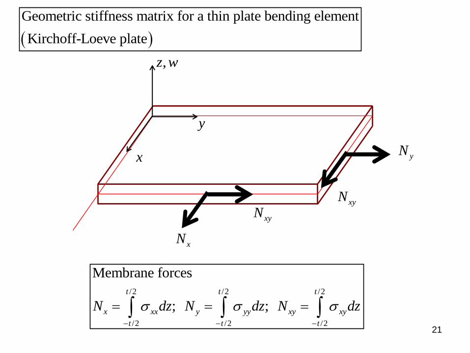
Geometric stiffness matrix for a thin plate bending element
Kirchoff-Loeve plate
x
,z w
y
yN
xyN
xyN
xN
/2 /2 /2
/2 /2 /2
Membrane forces
; ;
t t t
x xx y yy xy xy
t t t
N dz N dz N dz

22
Idea: examine the work done by the constant membrane forces on the
displacements associated with transverse deflections.
Membrane strains associated with small rotations & are given by
1
2xx
w w
x y
w
x
22
22
1; ; 2
2
Assume: , , are independent of ,
2
1 1
2 2
yy xy
x y xy
x xx y yy xy xy
A
x y xy
A
w w w
y x y
N N N w x y
U N N N dA
w w w wN N N dA
x y x y
w N
e e
w
xu G u
w
y

23
1
Isoparametric formulation
&
: matrix of derivatives of shape fun
e e
t x xy
xy y
I e
I
w
xw N u G u
w
y
N Nk G G dxdy
N N
w ww
xG u J
ww w
y
G
1 1
1 1
1 1
ctions wrt &
tt x xy
I I
xy y
N Nk G J J G d d
N N

24
1 1
1 1
1 1
Remarks
Membrane forces may vary in space and these variations may be accounted
for while evaluating the above integral
do not depend upon elastic prop
tt x xy
I I
xy y
N Nk G J J G d d
N N
k
erties of the plate (except to the extent
that these properties influence the initial membrane stresses that prevail).
The formulation can therefore be used for anisotropic material as well.

2 22
0
22 2
2 2
3D Timoshenko beam
1{
2
+ }
1
2
I
ly z
I y z
xy z z y x
yzx y
U U U
uU AE EI EI
x x x
v wGF GF GI dx
x x x
v wU N M
x x x
0
0
0
1
2
l
z
l
y x z x
l
y z z y x
dxx
v wM M dx
x x x x
M M
A V Perelmuter, CVslivker, 2013, Handbook of mechanical stability in engineering,
Vol.2, Stability of elastically deformable mechanical systems, World Scientific, New Jersey.

26
Imperfection sensitive structures
P PP
1k
2k
3k
A AA
B BB
I II III
l

27
1 2 3
12 3
A thought experiment
Design I,II and III in such a way that .
That is, select the spring constants , ,& such that .
It can be verified that , ,& cos
cI cII cIII
cI cII cIII
cI cII cIII
P P P
k k k P P P
kP P k l P k l
l
2
211 2 3 2 3
.
Thus, we are selecting , ,& such that cos .
If we were to fabricate the three models and perform experiments
it would be obeserved that no matter how carefully
the thre
cI cII cIII
kk k k k l k l
l
P P P
e models are fabricated and no matter how deligently the
experiments are performed.
It would also be observed that the scatter in the experimentally determined
value of critical loads would be such that
III II I
Scatter Scatter Scatter .
Indeed such behavior has been observed for the case when
I=beam, II=plate, and III=shell.

28
P
k A
B
I
P
2
2
2
2
11 cos
2
Equillibrium: 0 sin 0sin
Stability: 0 cos 0
Let the spring remain unstrained till > .
1cos cos
2
Equillibrium: 0 sin 0
V k Pl
V kk Pl P
l
Vk Pl
V k Pl
Vk Pl
Ideal
Imperfect
2
2
sin
Stability: 0 cos 0
kP
l
Vk Pl

29 -1.5 -1 -0.5 0 0.5 1 1.5
0
1000
2000
3000
4000
5000
6000
7000
theta
load P
Stable if
cos 0k Pl
Black: stableRed: Unstable
0
50
0
50

30
Remarks
Load-displacement curve for imperfect system rises
along a stable path without encountering any instability.
The deflection grows more rapidly as the load approaches
the critical value correspo
nding to a perfect system.
This is an example of a symmetric stable bifurcation
Beam structures display this type of behavior.

P
k
A
B
II
2
2
2
22 2
2
22
1sin 1 cos
2
Equillibrium: 0 sin cos sin 0
sin cos 0
Stability: 0 cos cos sin cos 0
Let the spring remain unstrained till > .
1sin sin
2
V k l Pl
Vkl Pl
kl Pl
Vkl Pl kl
V kl
Ideal
Imperfect
2
22
2
2
cos cos
Equillibrium: 0 sin sin cos sin 0
sin sin cos
sin
Stability: 0 cos sin sin sin cos 0
Pl
Vkl Pl
klP
Vkl Pl

32 -1.5 -1 -0.5 0 0.5 1 1.5
0
1000
2000
3000
4000
5000
6000
7000
theta
Load,P
Black: stableRed: Unstable
0 / 50
/ 20

33
Remarks
Load-displacement curve for imperfect system is not
always rising and stable; instead, it rises along a stable branch
and exhibits a limit point beyond which the path drops and becomes
unstable.
Greater the imperfection, lesser is the ability of structure to
carry the load.
This is an example of a symmetric unstable bifurcation
Plate structures display this type of behavior.

34
P
k
A
BP
B
O
cosL
cotL sinL
L
OB
OB
sinsin
s
s
L Ls
s
Structure is asymmetric

35
2
22 2 2
22 2 2
2 2 2
12 2 2 2
11 cos
2
sin
cot sin cos
1cot sin cos 1 cos
2 sin
Equillibrium: 0
cot sin cossin
1cot sin cos 2 cot sin
2
V k s s PL
Ls
s L L L
LV k L L L PL
V
V Lk L L L
L L L L L L
Ideal
2
2
2
cos 2 cos sin
sin
stability: 0
L
PL
V

36
P P
S
S
S
SUU
US

37
Remarks
The stable equillibrium path is asymetric with respect to the
undeflected configuration state wrt which the bifurcation takes place.
The stable load-displacement curve for imperfect system is
not
always rising and stable; instead, it rises along a stable branch
and exhibits a limit point beyond which the path drops and becomes
unstable.
Greater the imperfection, lesser is the ability of stru cture to
carry the load.
This is an example of an asymmetric unstable bifurcation
Shells (and frame) structures display this type of behavior.

38
Imperfection sensitive structures
P PP
1k
2k
3k
A AA
B BB
I II III
l
mP
mP

39
Illustrates the possibility of diverse type of behavior which could
be displayed by different structures.
The function encapuslates different types of structures.
can be expanded in Taylor's ser
U
U
ies about the equillibrium point
and different bifurcation patterns can be discerned by examining the
signs of various terms (Koiter's theory)
Nonlinear analysis helps us to examine the likely importanc e of geometric
imperfections in a given context.

Consider a simply supported, axially loaded beam on Winkler's foundation.
Reaction proportional to deflection
Same in tension and compression
Behaves like a series of springs
Beam on elastic foundation
(linear, elastic) without mutual interactions.
,EI lP P
k
2 22
2
2
0 0 0 0
4 2
4 2
1 1
2 2 2
0
BCs: Either 0 or 0 & Either 0 or 0
l l l ld y P dy
U EI dx dx ky dx p x y x dxdx dx
d y d yEI P ky
dx dx
y EIy Py y EIy

41
4 2
4 2
1
4
Consider a simply supported, axially loaded beam on Winkler's foundation.
0
0 0, 0, 0 0, 0
sinN
n
m
d y d yEI P ky
dx dx
y y L y y L
m xy x a
L
m mEI P
L
Simply supported beam on elastic foundation
2
2
2
0
Note: Notice the presence of in the denominator.
1 need not lead to the lowest critical load.
cr
kL
m kP EI
L m
L
m
m

42
2 2
2 2
3
,min
Smallest value of need not lead to the smallest value of .
is the smallest when 0
2 2 0
2 th
cr
cr
cr cr
cr
m P
m mP m EI k
L L
dP m P m
dm
k m kEI m
L L L EIm
L
k EIP EI k kEI
EI k
is value is independent of m
1P1P
2P2P
2 1
Special featureIt is possible that P P

43 101
102
103
104
105
106
108
109
1010
1011
1012
(l/r)2
Pcr
m=1
m=2
m=3
m=4
2 kEI

44
Exercise
Consider an Euler-Bernoulli beam element resting on a Winkler's
foundation. Develop the elastic and geometric stiffness matrices
for the element. Using the element thus developed determine
the critical load for a simply supported beam and illustrate the
results shown in the figure on the previous slide.

45
O
R
A
B
m
n1n
1m
1mm w
d
1 1
Buckling of a ring
=radius of the ring
AB=deformed configuration
mn=section of length in the undeformed
configuration
1
Upon deformation the section mn
becomes m n
Let =radius of the def
R
ds
dds Rd
ds R
1
ormed configuration
1
angle between tangent to the centre
at m and the perpendicular to the radius mO
d d
ds ds
dw
ds

46
1
2
1 2
2
2
1 1
angle between tangent to the centre at m and the perpendicular to the
radius mO
The corresponding angle at n is
Length m n :
1
dw
ds
dw d wds
ds ds
d wd ds
ds
dsds Rd R w d R w d ds wd w
R
d d
2 2
12 2
2 2 2
2 2 2 2
2 2 2
2 2 2
11
11 is ignored
1 1
d w d wd ds d ds
wds dsdsds ds ds R
ds wR
d d w w w d w w d w
ds ds R R R ds R ds
M w d w d w MRw
R EI R ds d EI

47
Ring under
Uniform
External
pressure
0 0
2 2 2
0 02
0, ,
hoop force=
w w M M
qR
d w MR Rw M qR w w
d EI EI
q
Ring with radius and thickness
Rh
Find critical value of pressure at which a neghbouring equillibrium (red) becomes possible
q

48
2 2
0 02
2 3 2
0 02
2 2 32 2
0 02
2
0 02
1
with 1
cos sin
sin cos
d w Rw M qR w w
d EI
d w qR Rw M qRw
d EI EI
d w R qRk w M qRw k
d EI EI
Rw A k B k M qRw
k EI
dwAk k Bk k
d

49
3
3
sin cos
For the mode shape we are looking for,
0 at =0, by symmetry2
0 at =0 0
0 at = sin 0 2,4,6...2 2
31 4c
c
dwAk k Bk k
d
dw
d
dwB
d
dw kk
d
q R EIq
EI R
Exercise: Using Euler-Bernoulli beam elements, verify this result.